A Three-County Regional Housing Needs Assessment:

A Three-County Regional Housing Needs Assessment:

Dutchess, Orange and Ulster Counties From 2006 to 2020

February 2009 Prepared By the Planning Departments of Dutchess, Orange, and Ulster Counties of New York With Project Consultation from Economic & Policy Resources, Inc.

Table of Contents

Executive Summary ..........................................................................................1 1. Introduction....................................................................................................3 2. Assessing Housing Affordability ....................................................................5

2.1 Affordability Calculations..........................................................................5 2.2 Housing Wage Analysis ...........................................................................9 2.3 Special Analysis: SWOT Interviews.........................................................9

3. U.S. Economic Outlook ...............................................................................11 3.1 The U.S. Housing Market and the Economy..........................................12 3.2 Financial Markets...................................................................................13 3.3 Energy Prices ........................................................................................15 3.4 Looking Forward ....................................................................................16

4. Housing Market Trends in the 3-County Region..........................................17 4.1 Housing Market Analysis Through June of 2007 ...................................17 4.2 Update on Housing Market Through September of 2008 ......................19 4.3 Affordability Pressures 1996 to 2006 .....................................................20

5. Economic and Demographic Forecasts, 2006 to 2020................................24 5.1 Economic Variables ...............................................................................24 5.2 Demographic Variables..........................................................................26

6. Current Housing Units Needed, 2006..........................................................29 6.1 Affordability Gap Analysis ......................................................................29 6.2 Municipal Allocations .............................................................................31

7. Prospective Housing Units Needed, 2006 to 2020......................................34 8. Targets for Building Affordable Housing......................................................39

8.1 Strategies to Address Affordability Challenges ......................................39 8.2 Build Targets to Address the 2006 Affordability Gap .............................40 8.3 Build Targets to Address the Prospective Demand ...............................41 8.4 Price and Rent Points Corresponding to the Build Targets....................44 8.5 County Level Build Numbers Distributed to the Municipalities ...............46

9. Conclusions.................................................................................................50 Appendix A. Project Flow Chart.......................................................................53 Appendix B. Economic and Demographic Forecast Tables ............................54 Appendix C. Housing Unit Demand Projections ..............................................62 Appendix D. Affordability Calculations in Detail...............................................67 Appendix E. Calculation of Municipal Median Household Income...................73 Appendix F. Municipal Allocations...................................................................77 Appendix G. Housing Wage Analysis..............................................................81 Appendix H. SWOT Analysis for the 3-County Region....................................92 Appendix I. Supplemental Analysis: the Age Group 55 Year and Over.........106 Appendix J. Calculation of Energy Price Impact............................................107 Appendix K. Glossary of Terms.....................................................................108 Appendix L. Affordability Calculation Tables By Municipality ........................110

About the Study This housing needs assessment study was initiated in the Summer of 2007 and was completed over the course of one and a half years. The Planning Departments of Dutchess, Orange and Ulster Counties decided to pursue a joint housing needs assessment due to the strong regional economic linkages between the Counties and the shared housing affordability challenges. The three Counties are inextricably linked through their relationship with the New York City Metro area, which brings both benefits (in terms of employment and business opportunities) and costs (through higher living expenses, transportation challenges, and an influx of new residents from the New York City area). The Counties also share similar challenges in meeting the affordable housing needs of their residents, an issue that was exacerbated by the housing market expansion from 2000 to 2006. As house prices increased rapidly during this period, household incomes also increased but not at a rate fast enough to keep pace with house prices. The regional economy has also been challenged to adapt with a changing global economy, in which workers in the three Counties are competing not only with workers in other states, but also with workers in other countries and dramatic technological improvements. Manufacturing job losses in the region have been offset with job gains in the services sector, but these service sector jobs typically pay lower wages. The three Counties also share the common experience of planning and developing transportation corridors suitable to meet the needs of regional commuters, both those traveling between the counties and for those who work in the New York City area. A substantial number of workers commute to jobs outside of their respective home County: 30.8% in Dutchess County, 34.5% in Orange County, and 33.5% in Ulster County, according to the 2000 Census. Coordinating what has been described as a fragmented transportation system, has become a priority of regional planning leaders, and also has implications for future affordable housing needs. This study represents an effort to develop a regional mindset in addressing housing affordability issues in the three Counties, encouraging elevated and more informed discussion, and joint planning where commonalities make coordination logical. However, recognizing that differences between the counties exist, such as geography, planning priorities and local regulations, it is also important to note that each of the Counties will likely find that solutions work with different degrees of success, and no single approach to address housing affordability issues is recommended in this study. In October of 2008, the New York State Division of Housing and Community Renewal (DHCR) released the Mid-Hudson Regional Report, a section of the overall Statewide Affordable Housing Needs Study. The report consisted of a series of focus group discussions with community stakeholders and housing

advocates from the three Counties covered in this study, plus Putnam and Sullivan Counties. The timing of the release of the DHCR report is rather fortunate, as it served as an appropriate preface to this needs assessment study. The DHCR report offered a qualitative view of affordability challenges in the region, including comments and observations on housing quality and conditions, diversity in the housing stock, and local community resistance to affordable housing development (also referred to as the NIMBY attitude, or Not In My Backyard). This housing needs assessment study completed by Dutchess, Orange and Ulster Counties is quantitative in content and can serve to supplement the DHCR report by providing local planners and decision makers with data, and where little or no data exist, carefully developed and thoroughly vetted estimates were made. Funding for this study was generously provided by the Dyson Foundation of Millbrook, NY. The study participants are listed below. Their participation and counsel was much appreciated over the course of the project. Dutchess County Roger P. Akeley, Commissioner, Dutchess County Department of Planning and Development Anne Conroy, Dutchess County Economic Development Corporation Ed Murphy, Associate Executive Director, Hudson River Housing Anne Saylor, Planner and Housing Coordinator, Dutchess County Department of Planning Ulster County Virginia Craft, Senior Planner, Ulster County Department of Planning Dennis Doyle, Commissioner, Ulster County Department of Planning Kevin O’Connor, Rural Ulster Preservation Company Joan Eck, Ulster Savings Bank Steve Aaron, Birchez Associates Michael Berg, Family of Woodstock Orange County Dave Church, Commissioner, Orange County Department of Planning Tony Figueroa, RECAP Inc. and Chair, OC Housing Consortium Kathy Murphy, Planner, Orange County Department of Planning Nancy Proyect, Exec Director, Orange County Citizens Foundation Gerald Jacobowitz Esq., Partner, Jacobowitz & Gubits Sandy Leonard, Supervisor, Town of Monroe

Regional Advisor Jonathan Drapkin, Patterns for Progress Project Consulting Team from Economic & Policy Resources, Inc Jeffrey Carr, President and Economist Zachary Sears, Research Economist Nonna Aydinyan, Economic Research Associate Nathan Johnson, Economic Research Associate Adam Bestenbostel, Research Assistant Justin Irving, Research Assistant

1

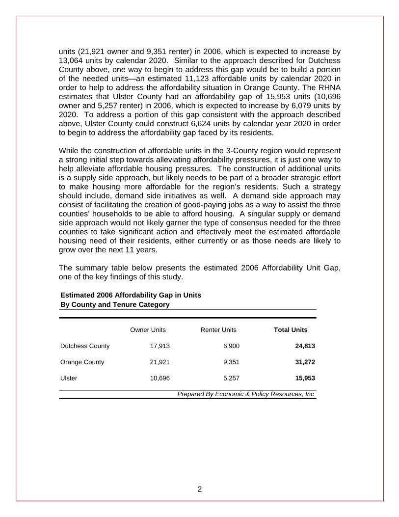
Executive Summary Some of the region’s residents in Dutchess, Orange and Ulster Counties are currently experiencing housing affordability challenges. The housing market expansion that began in the late 1990s and continued to 2006 contributed to the current housing affordability situation. During that time period, house prices grew at average rates of approximately 10% per year, while median household income grew at less than 4% per year. The three Counties also experienced substantial in-migration from the New York City area, as New York City residents sought cheaper, and for some safer, housing outside of the immediate metro area. Finally, another factor contributing to housing affordability issues in the region is community resistance to, and negative perceptions surrounding, affordable housing development. This Regional Housing Needs Assessment (RHNA) examined the current need for affordable housing in the 3-County region, using 2006 as the base year (the last full year of data available at the beginning of the study). Forecasts were also made of the expected need for affordable housing over the study period from 2006 to 2020. After quantifying the need for affordable housing, an estimate was made for the number of affordable units that each County will need to construct from 2006 to 2020 in order to address the current and expected affordable housing needs. The quantitative analysis was conducted by tenure category, for owners and renters, and also by income category relative to the County median household income – 50%, 80%, 100% and 120% of median household income for each respective County. The recent downturn in the U.S. housing market, which began to play out as this RHNA progressed, played an important role in the analysis. The economic and demographic forecast, a foundation piece for the assessment, accounted for events in the housing market and the broader U.S. recession. The forecast expects a period of restrained growth and declining or flat house prices out to 2010. House price declines are expected to alleviate some affordability pressures in the 3-County region, but not to the same extent that the price run-up added to those pressures. Therefore, despite some temporary relief in the near-term, affordability pressures are expected to continue to burden residents in the 3-County region over the time horizon of the RHNA, or through to 2020. Overall, it is estimated that in 2006 Dutchess County had a total affordability gap of 24,813 units (17,913 owner and 6,900 renter). From 2006 to 2020, this gap is expected to increase by 7,648 units. One way to begin to address this affordability gap would be to build a portion of this affordability gap—an estimated 9,372 affordable units by calendar 2020. This portion was derived based on the demographic trend of a declining average household size, and the additional pressure that is placed on the housing stock as a result of this trend in all three counties. Orange County’s 2006 affordability gap is estimated at 31,272

2

units (21,921 owner and 9,351 renter) in 2006, which is expected to increase by 13,064 units by calendar 2020. Similar to the approach described for Dutchess County above, one way to begin to address this gap would be to build a portion of the needed units—an estimated 11,123 affordable units by calendar 2020 in order to help to address the affordability situation in Orange County. The RHNA estimates that Ulster County had an affordability gap of 15,953 units (10,696 owner and 5,257 renter) in 2006, which is expected to increase by 6,079 units by 2020. To address a portion of this gap consistent with the approach described above, Ulster County could construct 6,624 units by calendar year 2020 in order to begin to address the affordability gap faced by its residents. While the construction of affordable units in the 3-County region would represent a strong initial step towards alleviating affordability pressures, it is just one way to help alleviate affordable housing pressures. The construction of additional units is a supply side approach, but likely needs to be part of a broader strategic effort to make housing more affordable for the region’s residents. Such a strategy should include, demand side initiatives as well. A demand side approach may consist of facilitating the creation of good-paying jobs as a way to assist the three counties’ households to be able to afford housing. A singular supply or demand side approach would not likely garner the type of consensus needed for the three counties to take significant action and effectively meet the estimated affordable housing need of their residents, either currently or as those needs are likely to grow over the next 11 years. The summary table below presents the estimated 2006 Affordability Unit Gap, one of the key findings of this study. Estimated 2006 Affordability Gap in UnitsBy County and Tenure Category

Owner Units Renter Units Total Units

Dutchess County 17,913 6,900 24,813

Orange County 21,921 9,351 31,272

Ulster 10,696 5,257 15,953

Prepared By Economic & Policy Resources, Inc

3

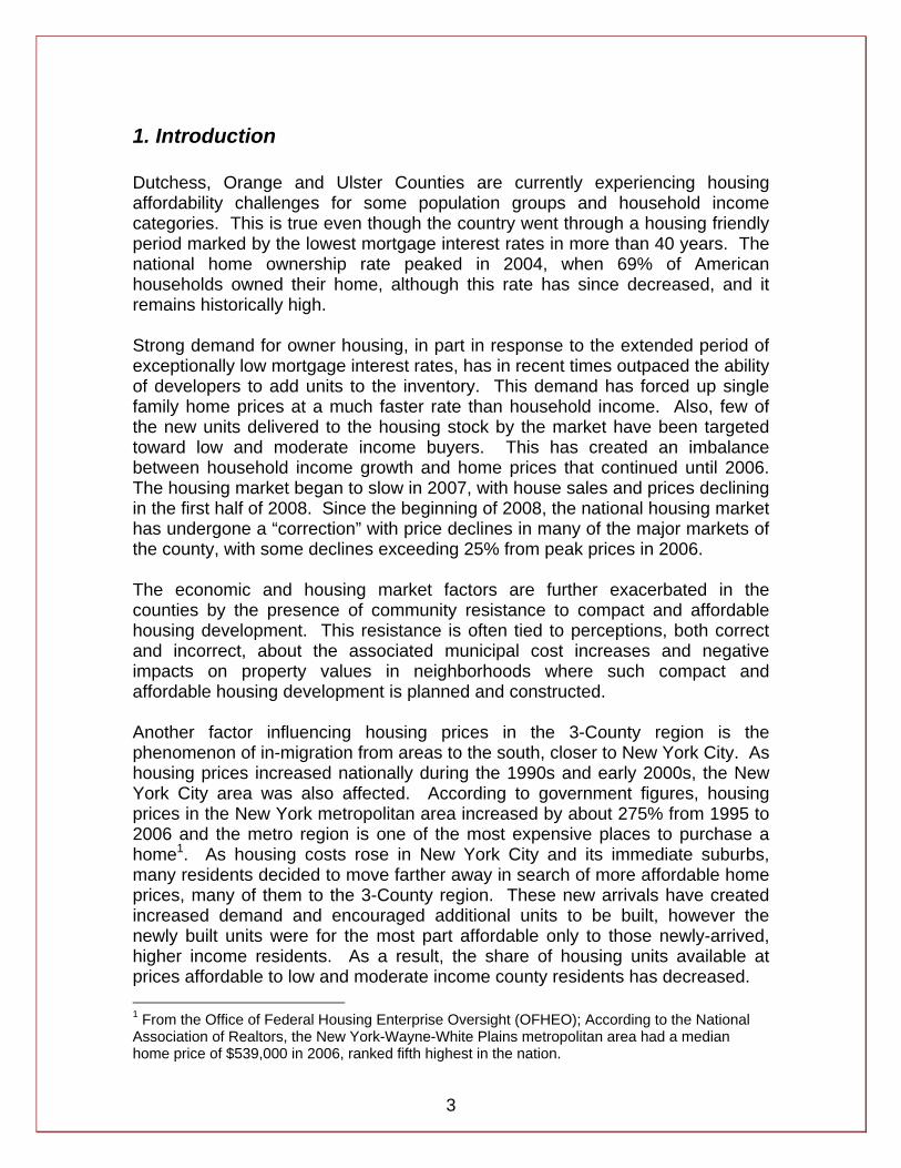
1. Introduction Dutchess, Orange and Ulster Counties are currently experiencing housing affordability challenges for some population groups and household income categories. This is true even though the country went through a housing friendly period marked by the lowest mortgage interest rates in more than 40 years. The national home ownership rate peaked in 2004, when 69% of American households owned their home, although this rate has since decreased, and it remains historically high. Strong demand for owner housing, in part in response to the extended period of exceptionally low mortgage interest rates, has in recent times outpaced the ability of developers to add units to the inventory. This demand has forced up single family home prices at a much faster rate than household income. Also, few of the new units delivered to the housing stock by the market have been targeted toward low and moderate income buyers. This has created an imbalance between household income growth and home prices that continued until 2006. The housing market began to slow in 2007, with house sales and prices declining in the first half of 2008. Since the beginning of 2008, the national housing market has undergone a “correction” with price declines in many of the major markets of the county, with some declines exceeding 25% from peak prices in 2006. The economic and housing market factors are further exacerbated in the counties by the presence of community resistance to compact and affordable housing development. This resistance is often tied to perceptions, both correct and incorrect, about the associated municipal cost increases and negative impacts on property values in neighborhoods where such compact and affordable housing development is planned and constructed. Another factor influencing housing prices in the 3-County region is the phenomenon of in-migration from areas to the south, closer to New York City. As housing prices increased nationally during the 1990s and early 2000s, the New York City area was also affected. According to government figures, housing prices in the New York metropolitan area increased by about 275% from 1995 to 2006 and the metro region is one of the most expensive places to purchase a home1. As housing costs rose in New York City and its immediate suburbs, many residents decided to move farther away in search of more affordable home prices, many of them to the 3-County region. These new arrivals have created increased demand and encouraged additional units to be built, however the newly built units were for the most part affordable only to those newly-arrived, higher income residents. As a result, the share of housing units available at prices affordable to low and moderate income county residents has decreased. 1 From the Office of Federal Housing Enterprise Oversight (OFHEO); According to the National Association of Realtors, the New York-Wayne-White Plains metropolitan area had a median home price of $539,000 in 2006, ranked fifth highest in the nation.

4

The costs of home ownership in the 3-County region have risen significantly over the last seven to eight years, with the median sale price of a single family home increasing by about 140% or more since 1996 in all three of the counties2.

Dutchess County: The median single family home sales price rose from $135,000 in 1996 to $330,000 in 2006, an increase of 144%, or 9.3% per year. Substantial percentage increases, in the double digits, began in 2001 and continued until 2005. While there was some variation in this trend at the municipal level, most of the 22 municipalities followed this pattern of relatively flat or slightly increasing prices through the 1990s, and then sharp price increases beginning in 2001.

Orange County: The median single family home price in Orange County

increased from $124,900 in 1996 to $298,500 in 2006. This represents a 139% increase overall, or an average annual increase of 9.1%. Again, the data show that prices at both the county and municipal level began to increase sharply around 2001.

Ulster County: House prices in Ulster County followed a similar trend

over the same time period: the median single family home price increased from $95,000 in 1996 to $244,665 in 2006. This is an increase of 157% over the 11 year period, or 9.9% per year. For 20 of the county’s 22 municipalities, trends mirror those in Dutchess and Orange Counties.

2 Median prices are calculated using NY ORPS data. The prices differ from published NY ORPS figures due to the inclusion of condo units in the medians reported here, while condo units are excluded from the calculation of NY ORPS medians.

5

2. Assessing Housing Affordability

2.1 Affordability Calculations The affordability analysis presented in the RHNA is based on U.S. Department of Housing and Urban Development (HUD) guidelines. Owner occupied housing is affordable if not more than 30% of a household’s gross income is spent on a mortgage payment, utilities, taxes, and insurance.3 For renter units, the HUD standard is that no more than 30% of a renter household’s income should be spent on rent and utilities (including fuel for heat, hot water and cooking, electricity for lights, water and waste water charges, and trash removal). An affordable house price was determined through the following steps: an affordable monthly housing payment was calculated by dividing median annual household income by 12 and then multiplying by 30%, following HUD guidelines. Insurance costs and property taxes were estimated and deducted from this affordable monthly housing payment, resulting in an amount available to “affordably” pay a monthly mortgage. Based on this affordable mortgage payment, an affordable house price was calculated assuming a fixed interest rate, a private mortgage insurance rate, and a 30-year loan term. These calculations allowed us to determine the value of a house that could be purchased, given a certain income level, without a household being housing-cost stressed. Tables 1 to 3a below, show calculations of affordable home prices by income group, displaying the median house price in each county, and the resulting affordability gaps in price (the difference between the median house price and the affordable house price for each respective income category). Clearly, in all three counties, many households had to choose between either foregoing a house purchase, or going ahead with a purchase but almost certainly becoming housing cost-stressed, that is, making housing payments that exceeded the 30% threshold. In Dutchess County, a household earning 120% of the household median income could afford a house worth $233,003, which was still shy of the median house price by almost $97,000. The median income household was $135,831 shy of the median priced house. The table also shows the number of houses available at or below the affordable price for each income group – again, even at 120% of the median household income, only 791 of 2924 sales would be considered affordable. This represents 27.1% of the total number of sales. The affordability gap increases at the lower income levels and the number of houses available 3 Consistent with the consensus of the study technical review committee, owner utility costs were not included in the owner affordability calculations in order to remain consistent with guidelines for some federal and state housing programs. Utilities were included in the calculations of the affordable rent.

6

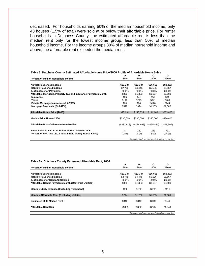
decreased. For households earning 50% of the median household income, only 43 houses (1.5% of total) were sold at or below their affordable price. For renter households in Dutchess County, the estimated affordable rent is less than the median rent only for the lowest income group, less than 50% of median household income. For the income groups 80% of median household income and above, the affordable rent exceeded the median rent. Table 1. Dutchess County Estimated Affordable Home Price/2006 Profile of Affordable Home Sales

A B C DPercent of Median Household Income 50% 80% 100% 120%

Annual Household Income $33,334 $53,334 $66,668 $80,002Monthly Household Income $2,778 $4,445 $5,556 $6,667% of Income for Payments 30.0% 30.0% 30.0% 30.0%Affordable Mortgage, Property Tax and Insurance Payments/Month $833 $1,333 $1,667 $2,000 Insurance $25 $41 $51 $61 Taxes $170 $273 $341 $409 Private Mortgage Insurance (@ 0.78%) $60 $96 $120 $144 Mortgage Payments (@ 6.41%) $578 $924 $1,155 $1,386

Affordable Home Price (2006) $97,084 $155,335 $194,169 $233,003

Median Price Home (2006) $330,000 $330,000 $330,000 $330,000

Affordable Price-Difference from Median ($232,916) ($174,665) ($135,831) ($96,997)

Home Sales Priced At or Below Median Price in 2006 43 120 233 791Percent of the Total (2924 Total Single Family House Sales) 1.5% 4.1% 8.0% 27.1%

Prepared by Economic and Policy Resources, Inc. Table 1a. Dutchess County Estimated Affordable Rent, 2006


Annual Household Income $33,334 $53,334 $66,668 $80,002Monthly Household Income $2,778 $4,445 $5,556 $6,667% of Income for Rent and Utilities 30.0% 30.0% 30.0% 30.0%Affordable Renter Payments/Month (Rent Plus Utilities) $833 $1,333 $1,667 $2,000

Monthly Utility Expense (Excluding Telephone) $89 $102 $102 $111

Monthly Affordable Rent (Excluding Utilities) $744 $1,232 $1,565 $1,889

Estimated 2006 Median Rent $840 $840 $840 $840

Affordable Rent Gap ($96) $392 $725 $1,049

Prepared by Economic and Policy Resources, Inc.

7

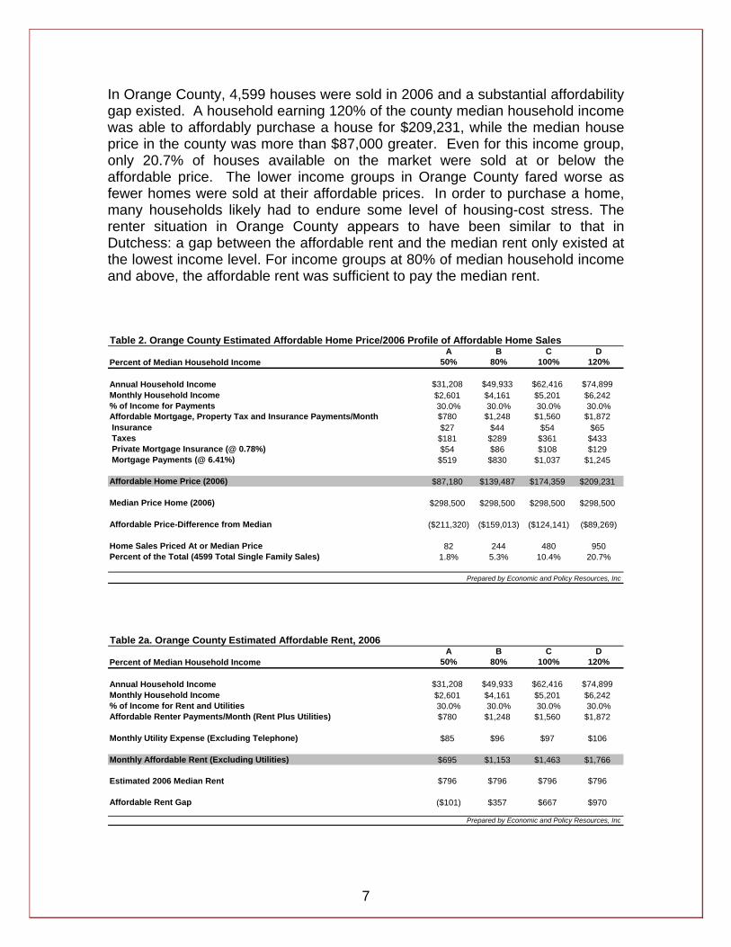
In Orange County, 4,599 houses were sold in 2006 and a substantial affordability gap existed. A household earning 120% of the county median household income was able to affordably purchase a house for $209,231, while the median house price in the county was more than $87,000 greater. Even for this income group, only 20.7% of houses available on the market were sold at or below the affordable price. The lower income groups in Orange County fared worse as fewer homes were sold at their affordable prices. In order to purchase a home, many households likely had to endure some level of housing-cost stress. The renter situation in Orange County appears to have been similar to that in Dutchess: a gap between the affordable rent and the median rent only existed at the lowest income level. For income groups at 80% of median household income and above, the affordable rent was sufficient to pay the median rent. Table 2. Orange County Estimated Affordable Home Price/2006 Profile of Affordable Home Sales






Home Sales Priced At or Median Price 82 244 480 950Percent of the Total (4599 Total Single Family Sales) 1.8% 5.3% 10.4% 20.7%

Prepared by Economic and Policy Resources, Inc Table 2a. Orange County Estimated Affordable Rent, 2006






Affordable Rent Gap ($101) $357 $667 $970

Prepared by Economic and Policy Resources, Inc

8

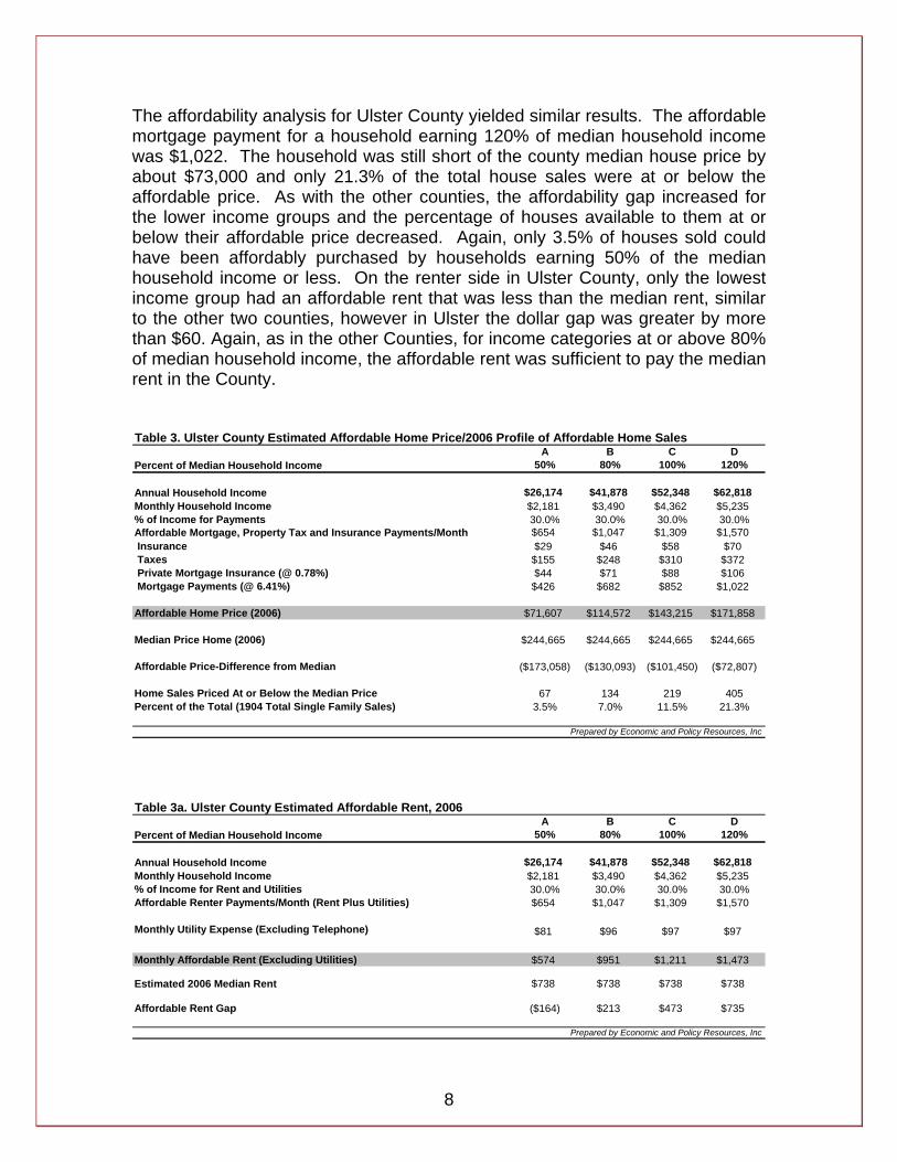
The affordability analysis for Ulster County yielded similar results. The affordable mortgage payment for a household earning 120% of median household income was $1,022. The household was still short of the county median house price by about $73,000 and only 21.3% of the total house sales were at or below the affordable price. As with the other counties, the affordability gap increased for the lower income groups and the percentage of houses available to them at or below their affordable price decreased. Again, only 3.5% of houses sold could have been affordably purchased by households earning 50% of the median household income or less. On the renter side in Ulster County, only the lowest income group had an affordable rent that was less than the median rent, similar to the other two counties, however in Ulster the dollar gap was greater by more than $60. Again, as in the other Counties, for income categories at or above 80% of median household income, the affordable rent was sufficient to pay the median rent in the County. Table 3. Ulster County Estimated Affordable Home Price/2006 Profile of Affordable Home Sales


Annual Household Income $26,174 $41,878 $52,348 $62,818Monthly Household Income $2,181 $3,490 $4,362 $5,235% of Income for Payments 30.0% 30.0% 30.0% 30.0%Affordable Mortgage, Property Tax and Insurance Payments/Month $654 $1,047 $1,309 $1,570 Insurance $29 $46 $58 $70 Taxes $155 $248 $310 $372 Private Mortgage Insurance (@ 0.78%) $44 $71 $88 $106 Mortgage Payments (@ 6.41%) $426 $682 $852 $1,022




Home Sales Priced At or Below the Median Price 67 134 219 405Percent of the Total (1904 Total Single Family Sales) 3.5% 7.0% 11.5% 21.3%

Prepared by Economic and Policy Resources, Inc Table 3a. Ulster County Estimated Affordable Rent, 2006




Monthly Affordable Rent (Excluding Utilities) $574 $951 $1,211 $1,473




9

This analysis was repeated for each city and town of the three counties, factoring in each municipality’s property taxes, median income, median house price, and assumed insurance rates and utility costs across municipalities. The analysis allowed an affordable house price and rent to be identified by income level for each municipality, and for the determination of the number of sales at or below each income group’s affordable price on the owner side. The affordability analysis for each municipality is presented in Appendix L on page 110

2.2 Housing Wage Analysis This section provides a brief description of a supplemental housing wage analysis that was completed in order to connect the abstract concept of housing affordability to the region’s labor market. Earnings in selected job sectors in the 3-County region were compared to the earnings necessary to affordably own a median priced house, or pay rent on a 2-bedroom apartment. Data from the Bureau of Labor Statistics’ Quarterly Census of Employment and Wages (QCEW) are used in the analysis, and allow for comparison between average earnings in various sectors of the regional labor market and the income necessary to avoid housing burden, or the housing wage. The analysis shows that in each of the three counties, the average wages in some major job sectors were not sufficient to affordably purchase a median priced home for a single earner household. Therefore, multiple wage earners would be needed in these sectors. The difference between the average wage and the housing wage is especially apparent on the owner side in the Accommodation and Food Services and Retail Trade Sectors. These sectors pay wages that would require a household to have seven wage earners in the household in Dutchess and Orange Counties, and five wage earners in Ulster County. The gaps in the average wage and housing wage are also apparent on the renter side, but to a lesser degree. The detailed housing wage analysis is available in this report as Appendix G on page 81.

2.3 Special Analysis: SWOT Interviews As part of this RHNA, a Strengths, Weaknesses, Opportunities, and Threats assessment (or what is commonly known as a SWOT) was conducted. Key regional stakeholders active in housing issues were identified in each county by the respective County Planning Departments. The interviews were conducted during late October-early November 2007. Those selected for interviews involved a broad range of participants in the regional housing arena including local government officials, non profit administrators, and private developers. The objectives of these interviews were: (1) to obtain a “reality check” on the data our analysis team had assembled, (2) to get a face to face description of the facts

10

and nuances of the situation “on the ground” including any possible constraints and/or opportunities, (3) to identify notable constraints to housing development in the region, and (4) to solicit ideas and insights to the housing market issues and identify housing market opportunities that could be of use following the completion of this RHNA. While there are many findings of note in this SWOT analysis, one general finding came clearly through from the interview process. SWOT respondents in various ways indicated that although the three County governments, several competent non-profit agencies and several private developers in the region understand the problem and are willing to take action, only a few of the municipalities outside of the region’s cities have shown a willingness to undertake necessary actions to address the region’s housing challenges. This condition will likely act as a general impediment to the development of housing in at least parts of the 3-County region. The final part of this SWOT assessment included the development of an inventory of ideas from stakeholders that could be used to jumpstart the development of an action agenda. Among the key necessary actions identified by SWOT respondents to address the regional housing challenges included: (1) housing-friendly adjustments to land use regulations, and (2) critical direct capital spending that would permit and/or encourage the development of housing that is affordable at the price points in the range of need identified by this assessment study. The full SWOT analysis is provided in Appendix H on page 92 of this report.

11

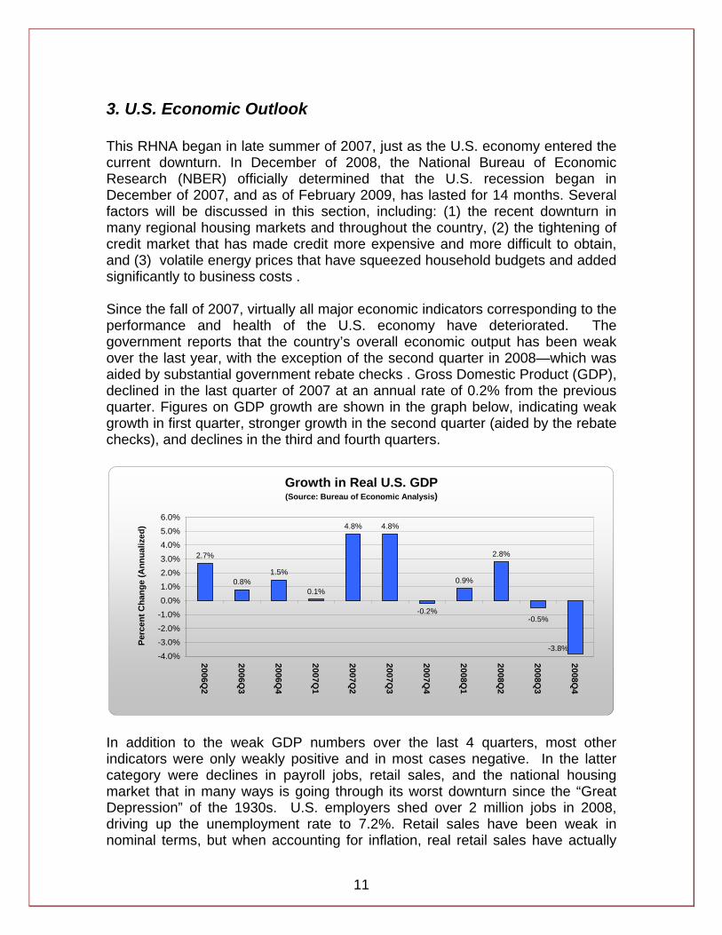
3. U.S. Economic Outlook This RHNA began in late summer of 2007, just as the U.S. economy entered the current downturn. In December of 2008, the National Bureau of Economic Research (NBER) officially determined that the U.S. recession began in December of 2007, and as of February 2009, has lasted for 14 months. Several factors will be discussed in this section, including: (1) the recent downturn in many regional housing markets and throughout the country, (2) the tightening of credit market that has made credit more expensive and more difficult to obtain, and (3) volatile energy prices that have squeezed household budgets and added significantly to business costs . Since the fall of 2007, virtually all major economic indicators corresponding to the performance and health of the U.S. economy have deteriorated. The government reports that the country’s overall economic output has been weak over the last year, with the exception of the second quarter in 2008—which was aided by substantial government rebate checks . Gross Domestic Product (GDP), declined in the last quarter of 2007 at an annual rate of 0.2% from the previous quarter. Figures on GDP growth are shown in the graph below, indicating weak growth in first quarter, stronger growth in the second quarter (aided by the rebate checks), and declines in the third and fourth quarters.

Growth in Real U.S. GDP(Source: Bureau of Economic Analysis)

2.7%

0.8%1.5%

0.1%

4.8% 4.8%

-0.2%

0.9%

2.8%

-0.5%

-3.8%-4.0%-3.0%-2.0%-1.0%0.0%1.0%2.0%3.0%4.0%5.0%6.0%

2006Q2

2006Q3

2006Q4

2007Q1

2007Q2

2007Q3

2007Q4

2008Q1

2008Q2

2008Q3

2008Q4

Perc

ent C

hang

e (A

nnua

lized

)

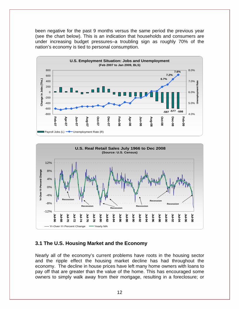
In addition to the weak GDP numbers over the last 4 quarters, most other indicators were only weakly positive and in most cases negative. In the latter category were declines in payroll jobs, retail sales, and the national housing market that in many ways is going through its worst downturn since the “Great Depression” of the 1930s. U.S. employers shed over 2 million jobs in 2008, driving up the unemployment rate to 7.2%. Retail sales have been weak in nominal terms, but when accounting for inflation, real retail sales have actually

12

been negative for the past 9 months versus the same period the previous year (see the chart below). This is an indication that households and consumers are under increasing budget pressures–a troubling sign as roughly 70% of the nation’s economy is tied to personal consumption.

U.S. Employment Situation: Jobs and Unemployment(Feb 2007 to Jan 2009, BLS)

-597 -577 -598

7.6%7.2%

6.7%

-800

-600

-400

-200

0

200

400

600

800

Feb-07

Apr-07

Jun-07

Aug-07

Oct-07

Dec-07

Feb-08

Apr-08

Jun-08

Aug-08

Oct-08

Dec-08

Feb-09

Cha

nge

in J

obs

(Ths

.)

4.0%

5.0%

6.0%

7.0%

8.0%

Une

mpl

oym

ent R

ate

Payroll Jobs (L) Unemployment Rate (R)

U.S. Real Retail Sales July 1966 to Dec 2008(Source: U.S. Census)

-12%

-8%

-4%

0%

4%

8%

12%

Jul-66

Jul-68

Jul-70

Jul-72

Jul-74

Jul-76

Jul-78

Jul-80

Jul-82

Jul-84

Jul-86

Jul-88

Jul-90

Jul-92

Jul-94

Jul-96

Jul-98

Jul-00

Jul-02

Jul-04

Jul-06

Jul-08

Yr-O

ver-

Yr P

erce

nt C

hang

e

Yr-Over-Yr Percent Change Yearly MA

Recession

RecessionRecession

Recession

RecessionRecession

3.1 The U.S. Housing Market and the Economy Nearly all of the economy’s current problems have roots in the housing sector and the ripple effect the housing market decline has had throughout the economy. The decline in house prices have left many home owners with loans to pay off that are greater than the value of the home. This has encouraged some owners to simply walk away from their mortgage, resulting in a foreclosure; or

13

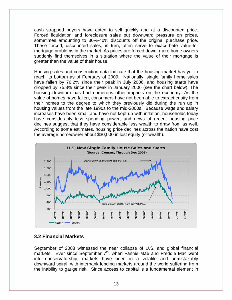
cash strapped buyers have opted to sell quickly and at a discounted price. Forced liquidation and foreclosure sales put downward pressure on prices, sometimes amounting to 30%-40% discounts off the original purchase price. These forced, discounted sales, in turn, often serve to exacerbate value-to-mortgage problems in the market. As prices are forced down, more home owners suddenly find themselves in a situation where the value of their mortgage is greater than the value of their house. Housing sales and construction data indicate that the housing market has yet to reach its bottom as of February of 2009. Nationally, single family home sales have fallen by 76.2% since their peak in July 2006, and housing starts have dropped by 75.8% since their peak in January 2006 (see the chart below). The housing downturn has had numerous other impacts on the economy. As the value of homes have fallen, consumers have not been able to extract equity from their homes to the degree to which they previously did during the run up in housing values from the late 1990s to the mid-2000s. Because wage and salary increases have been small and have not kept up with inflation, households today have considerably less spending power, and news of recent housing price declines suggest that they have considerable less wealth to draw from as well. According to some estimates, housing price declines across the nation have cost the average homeowner about $30,000 in lost equity (or wealth).

U.S. New Single Family House Sales and Starts (Source: Census, Through Dec 2008)

100

400

700

1,000

1,300

1,600

1,900

2,200

Jan-80

Jan-82

Jan-84

Jan-86

Jan-88

Jan-90

Jan-92

Jan-94

Jan-96

Jan-98

Jan-00

Jan-02

Jan-04

Jan-06

Jan-08

Jan-10

Jan-12

Thou

sand

s

Sales Starts

Sales Down 76.2% from July '05 Peak

Starts Down 75.8% from Jan '06 Peak

3.2 Financial Markets September of 2008 witnessed the near collapse of U.S. and global financial markets. Ever since September 7th, when Fannie Mae and Freddie Mac went into conservatorship, markets have been in a volatile and unmistakably downward spiral, with interbank lending markets around the world suffering from the inability to gauge risk. Since access to capital is a fundamental element in

14

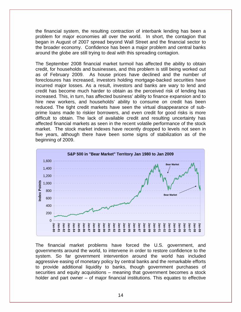
the financial system, the resulting contraction of interbank lending has been a problem for major economies all over the world. In short, the contagion that began in August of 2007 spread beyond Wall Street and the financial sector to the broader economy. Confidence has been a major problem and central banks around the globe are still trying to deal with this spreading contagion. The September 2008 financial market turmoil has affected the ability to obtain credit, for households and businesses, and this problem is still being worked out as of February 2009. As house prices have declined and the number of foreclosures has increased, investors holding mortgage-backed securities have incurred major losses. As a result, investors and banks are wary to lend and credit has become much harder to obtain as the perceived risk of lending has increased. This, in turn, has affected business’ ability to finance expansion and to hire new workers, and households’ ability to consume on credit has been reduced. The tight credit markets have seen the virtual disappearance of sub-prime loans made to riskier borrowers, and even credit for good risks is more difficult to obtain. The lack of available credit and resulting uncertainty has affected financial markets as seen in the recent volatile performance of the stock market. The stock market indexes have recently dropped to levels not seen in five years, although there have been some signs of stabilization as of the beginning of 2009.

S&P 500 in "Bear Market" Territory Jan 1980 to Jan 2009

0

200

400

600

800

1,000

1,200

1,400

1,600

Jan-80Jan-81Jan-82

Jan-83Jan-84Jan-85Jan-86Jan-87Jan-88Jan-89Jan-90

Jan-91Jan-92Jan-93Jan-94Jan-95Jan-96Jan-97Jan-98Jan-99Jan-00Jan-01Jan-02Jan-03Jan-04Jan-05Jan-06Jan-07

Jan-08Jan-09

Inde

x Po

ints

Bear Market

Bear Market

The financial market problems have forced the U.S. government, and governments around the world, to intervene in order to restore confidence to the system. So far government intervention around the world has included aggressive easing of monetary policy by central banks and the remarkable efforts to provide additional liquidity to banks, though government purchases of securities and equity acquisitions – meaning that government becomes a stock holder and part owner – of major financial institutions. This equates to effective

15

nationalization of many financial institutions. In addition, governments around the world have stepped in to insure bank deposits in various forms and amounts, in order restore confidence and prevent all out runs on the banks. In short, the developments in the global financial markets in September and October of 2008 have been nothing short of unprecedented and continue to affect the U.S. and global economies as of February 2009.

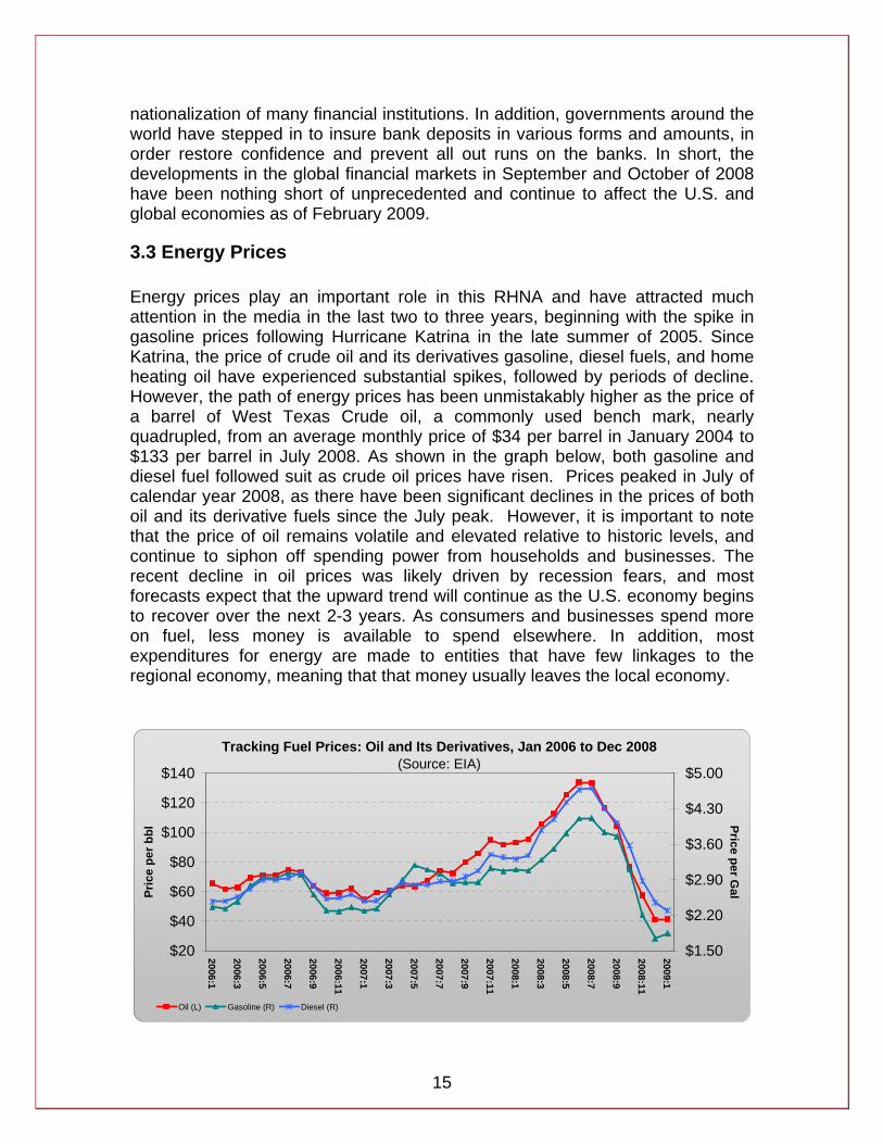
3.3 Energy Prices Energy prices play an important role in this RHNA and have attracted much attention in the media in the last two to three years, beginning with the spike in gasoline prices following Hurricane Katrina in the late summer of 2005. Since Katrina, the price of crude oil and its derivatives gasoline, diesel fuels, and home heating oil have experienced substantial spikes, followed by periods of decline. However, the path of energy prices has been unmistakably higher as the price of a barrel of West Texas Crude oil, a commonly used bench mark, nearly quadrupled, from an average monthly price of $34 per barrel in January 2004 to $133 per barrel in July 2008. As shown in the graph below, both gasoline and diesel fuel followed suit as crude oil prices have risen. Prices peaked in July of calendar year 2008, as there have been significant declines in the prices of both oil and its derivative fuels since the July peak. However, it is important to note that the price of oil remains volatile and elevated relative to historic levels, and continue to siphon off spending power from households and businesses. The recent decline in oil prices was likely driven by recession fears, and most forecasts expect that the upward trend will continue as the U.S. economy begins to recover over the next 2-3 years. As consumers and businesses spend more on fuel, less money is available to spend elsewhere. In addition, most expenditures for energy are made to entities that have few linkages to the regional economy, meaning that that money usually leaves the local economy.

Tracking Fuel Prices: Oil and Its Derivatives, Jan 2006 to Dec 2008(Source: EIA)

$20

$40

$60

$80

$100

$120

$140

2006:1

2006:3

2006:5

2006:7

2006:9

2006:11

2007:1

2007:3

2007:5

2007:7

2007:9

2007:11

2008:1

2008:3

2008:5

2008:7

2008:9

2008:11

2009:1

Pric

e pe

r bbl

$1.50

$2.20

$2.90

$3.60

$4.30

$5.00

Price per Gal

Oil (L) Gasoline (R) Diesel (R)S

16

The 3-County region has not escaped the adverse impact of elevated energy prices. An estimated $286.7 million was siphoned out of the regional economy by elevated petroleum prices in the first half of 2008, according to our estimates. When broken down by County, we estimate that Dutchess County spent an additional $98.5 million on petroleum, Orange County an additional $126.4 million, and Ulster County an additional $61.7 million, representing money that was taken out of the local economy.4

3.4 Looking Forward As announced in December 2008, the US economy is officially in a recession as of December 2007. The events in the national economy over the past year influenced the long term economic and demographic forecast for the 3-Counties in three important ways: (1) credit is expected to be more difficult to obtain in the near term period 2006-10, (2) energy prices are expected to remain at levels that are elevated relative to historic prices (despite the recent declines), and (3) the struggling economy will likely exacerbate relatively weak population growth forecasted in the region. Regarding the first, this means that achieving home ownership will likely be more difficult over the next several years, compared with the low interest rate period of the early 2000’s. Tighter credit could also mean that recovery from the current economic downturn will be slow and protracted, as businesses in the Hudson Valley, and the U.S. as a whole, struggle to find financing for expansion. Once the housing and financial market problems have run their course and begun to recover, the economy should eventually return to expansion at a level closer to its long term average rate of growth (roughly 2-3% per year in terms of GDP). Regarding the second, high energy prices will likely act as a drag on the economy unless or until new technologies are developed and implemented that that reduce energy usage and the nation’s reliance on fossil fuels. The above estimate of additional spending on petroleum is an example of how high energy prices siphon off money from the regional economy without any offsetting public spending.5 The third factor, slowing population growth, is a trend that can be observed in other regions in the northeast part of the country as well. The changing demographics imply that the next 15 years or so will likely be very different than the last 15 years, with relatively restrained economic growth expected.

4 See Appendix J for more details on this estimated impact of elevated petroleum prices in the 3-County region. 5 Offsetting public spending refers to taxes that siphon off money from households, but are at least accompanied by government spending. Increased energy prices reduce the amount that households spend and are not accompanied by any government spending that offset the reduced household spending.

17

4. Housing Market Trends in the 3-County Region

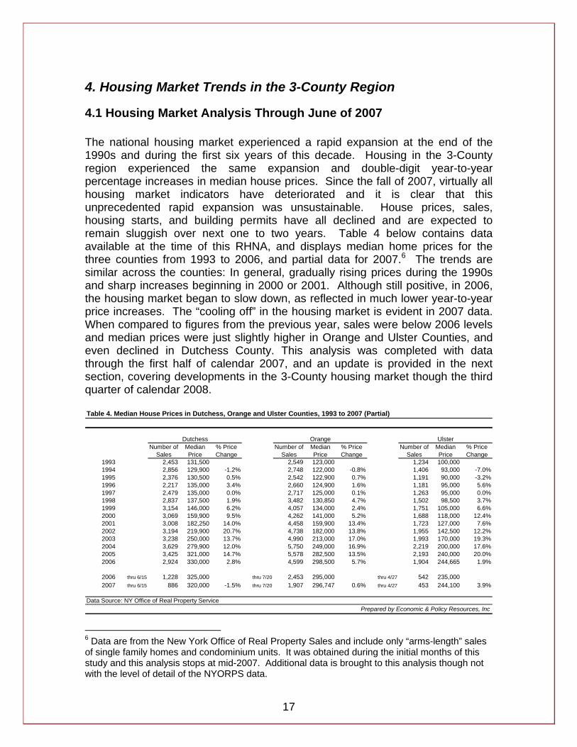
4.1 Housing Market Analysis Through June of 2007 The national housing market experienced a rapid expansion at the end of the 1990s and during the first six years of this decade. Housing in the 3-County region experienced the same expansion and double-digit year-to-year percentage increases in median house prices. Since the fall of 2007, virtually all housing market indicators have deteriorated and it is clear that this unprecedented rapid expansion was unsustainable. House prices, sales, housing starts, and building permits have all declined and are expected to remain sluggish over next one to two years. Table 4 below contains data available at the time of this RHNA, and displays median home prices for the three counties from 1993 to 2006, and partial data for 2007.6 The trends are similar across the counties: In general, gradually rising prices during the 1990s and sharp increases beginning in 2000 or 2001. Although still positive, in 2006, the housing market began to slow down, as reflected in much lower year-to-year price increases. The “cooling off” in the housing market is evident in 2007 data. When compared to figures from the previous year, sales were below 2006 levels and median prices were just slightly higher in Orange and Ulster Counties, and even declined in Dutchess County. This analysis was completed with data through the first half of calendar 2007, and an update is provided in the next section, covering developments in the 3-County housing market though the third quarter of calendar 2008. Table 4. Median House Prices in Dutchess, Orange and Ulster Counties, 1993 to 2007 (Partial)

Number of Sales

Median Price

% Price Change

Number of Sales

Median Price

% Price Change

Number of Sales

Median Price

% Price Change

1993 2,453 131,500 2,549 123,000 1,234 100,0001994 2,856 129,900 -1.2% 2,748 122,000 -0.8% 1,406 93,000 -7.0%1995 2,376 130,500 0.5% 2,542 122,900 0.7% 1,191 90,000 -3.2%1996 2,217 135,000 3.4% 2,660 124,900 1.6% 1,181 95,000 5.6%1997 2,479 135,000 0.0% 2,717 125,000 0.1% 1,263 95,000 0.0%1998 2,837 137,500 1.9% 3,482 130,850 4.7% 1,502 98,500 3.7%1999 3,154 146,000 6.2% 4,057 134,000 2.4% 1,751 105,000 6.6%2000 3,069 159,900 9.5% 4,262 141,000 5.2% 1,688 118,000 12.4%2001 3,008 182,250 14.0% 4,458 159,900 13.4% 1,723 127,000 7.6%2002 3,194 219,900 20.7% 4,738 182,000 13.8% 1,955 142,500 12.2%2003 3,238 250,000 13.7% 4,990 213,000 17.0% 1,993 170,000 19.3%2004 3,629 279,900 12.0% 5,750 249,000 16.9% 2,219 200,000 17.6%2005 3,425 321,000 14.7% 5,578 282,500 13.5% 2,193 240,000 20.0%2006 2,924 330,000 2.8% 4,599 298,500 5.7% 1,904 244,665 1.9%

2006 thru 6/15 1,228 325,000 thru 7/20 2,453 295,000 thru 4/27 542 235,0002007 thru 6/15 886 320,000 -1.5% thru 7/20 1,907 296,747 0.6% thru 4/27 453 244,100 3.9%

Data Source: NY Office of Real Property ServicePrepared by Economic & Policy Resources, Inc

Dutchess Orange Ulster

6 Data are from the New York Office of Real Property Sales and include only “arms-length” sales of single family homes and condominium units. It was obtained during the initial months of this study and this analysis stops at mid-2007. Additional data is brought to this analysis though not with the level of detail of the NYORPS data.

18

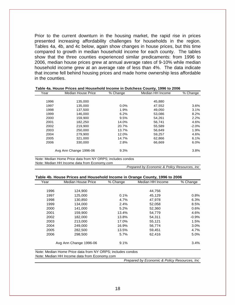
Prior to the current downturn in the housing market, the rapid rise in prices presented increasing affordability challenges for households in the region. Tables 4a, 4b, and 4c below, again show changes in house prices, but this time compared to growth in median household income for each county. The tables show that the three counties experienced similar predicaments: from 1996 to 2006, median house prices grew at annual average rates of 9-10% while median household income grew at an average rate of less than 4%. The data indicate that income fell behind housing prices and made home ownership less affordable in the counties. Table 4a. House Prices and Household Income in Dutchess County, 1996 to 2006

Year Median House Price % Change Median HH Income % Change

1996 135,000 45,8801997 135,000 0.0% 47,552 3.6%1998 137,500 1.9% 49,050 3.1%1999 146,000 6.2% 53,086 8.2%2000 159,900 9.5% 54,261 2.2%2001 182,250 14.0% 56,741 4.6%2002 219,900 20.7% 55,589 -2.0%2003 250,000 13.7% 56,649 1.9%2004 279,900 12.0% 59,257 4.6%2005 321,000 14.7% 62,866 6.1%2006 330,000 2.8% 66,669 6.0%

Avg Ann Change 1996-06 9.3% 3.8%

Note: Median Home Price data from NY ORPS; includes condosNote: Median HH Income data from Economy.com

Prepared by Economic & Policy Resources, Inc Table 4b. House Prices and Household Income in Orange County, 1996 to 2006

Year Median House Price % Change Median HH Income % Change

1996 124,900 44,7561997 125,000 0.1% 45,129 0.8%1998 130,850 4.7% 47,978 6.3%1999 134,000 2.4% 52,058 8.5%2000 141,000 5.2% 52,360 0.6%2001 159,900 13.4% 54,779 4.6%2002 182,000 13.8% 54,311 -0.9%2003 213,000 17.0% 55,121 1.5%2004 249,000 16.9% 56,774 3.0%2005 282,500 13.5% 59,451 4.7%2006 298,500 5.7% 62,416 5.0%

Avg Ann Change 1996-06 9.1% 3.4%


Prepared by Economic & Policy Resources, Inc

19

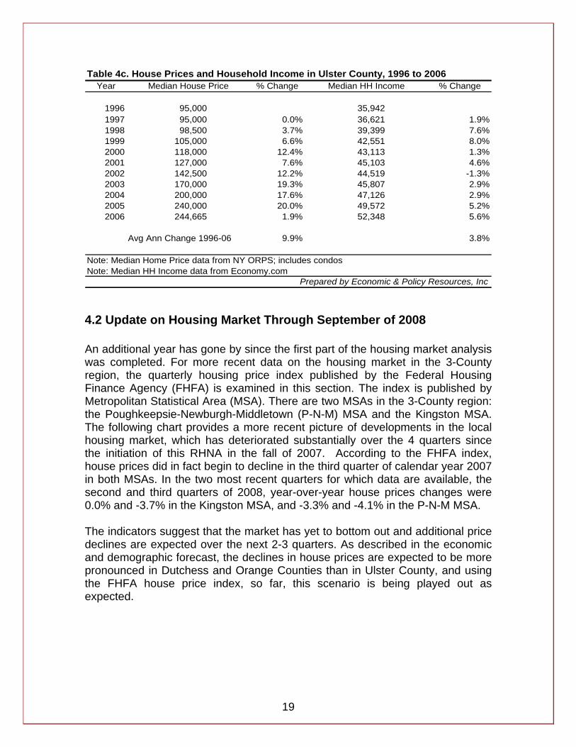
Table 4c. House Prices and Household Income in Ulster County, 1996 to 2006Year Median House Price % Change Median HH Income % Change

1996 95,000 35,9421997 95,000 0.0% 36,621 1.9%1998 98,500 3.7% 39,399 7.6%1999 105,000 6.6% 42,551 8.0%2000 118,000 12.4% 43,113 1.3%2001 127,000 7.6% 45,103 4.6%2002 142,500 12.2% 44,519 -1.3%2003 170,000 19.3% 45,807 2.9%2004 200,000 17.6% 47,126 2.9%2005 240,000 20.0% 49,572 5.2%2006 244,665 1.9% 52,348 5.6%

Avg Ann Change 1996-06 9.9% 3.8%


Prepared by Economic & Policy Resources, Inc

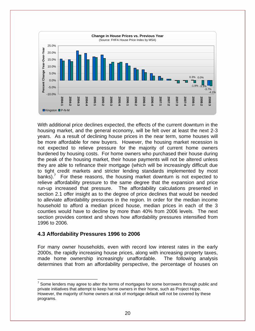
4.2 Update on Housing Market Through September of 2008 An additional year has gone by since the first part of the housing market analysis was completed. For more recent data on the housing market in the 3-County region, the quarterly housing price index published by the Federal Housing Finance Agency (FHFA) is examined in this section. The index is published by Metropolitan Statistical Area (MSA). There are two MSAs in the 3-County region: the Poughkeepsie-Newburgh-Middletown (P-N-M) MSA and the Kingston MSA. The following chart provides a more recent picture of developments in the local housing market, which has deteriorated substantially over the 4 quarters since the initiation of this RHNA in the fall of 2007. According to the FHFA index, house prices did in fact begin to decline in the third quarter of calendar year 2007 in both MSAs. In the two most recent quarters for which data are available, the second and third quarters of 2008, year-over-year house prices changes were 0.0% and -3.7% in the Kingston MSA, and -3.3% and -4.1% in the P-N-M MSA. The indicators suggest that the market has yet to bottom out and additional price declines are expected over the next 2-3 quarters. As described in the economic and demographic forecast, the declines in house prices are expected to be more pronounced in Dutchess and Orange Counties than in Ulster County, and using the FHFA house price index, so far, this scenario is being played out as expected.

20

Change in House Prices vs. Previous Year(Source: FHFA House Price Index by MSA)

0.3%

-3.7%

0.0%

-4.1%

-3.3%-1.9%

-10.0%

-5.0%

0.0%

5.0%

10.0%

15.0%

20.0%

25.0%

2004:1

2004:2

2004:3

2004:4

2005:1

2005:2

2005:3

2005:4

2006:1

2006:2

2006:3

2006:4

2007:1

2007:2

2007:3

2007:4

2008:1

2008:2

2008:3Pe

rcen

t Cha

nge

Year

-Ove

r-Ye

ar

Kingston P-N-M

With additional price declines expected, the effects of the current downturn in the housing market, and the general economy, will be felt over at least the next 2-3 years. As a result of declining house prices in the near term, some houses will be more affordable for new buyers. However, the housing market recession is not expected to relieve pressure for the majority of current home owners burdened by housing costs. For home owners who purchased their house during the peak of the housing market, their house payments will not be altered unless they are able to refinance their mortgage (which will be increasingly difficult due to tight credit markets and stricter lending standards implemented by most banks).7 For these reasons, the housing market downturn is not expected to relieve affordability pressure to the same degree that the expansion and price run-up increased that pressure. The affordability calculations presented in section 2.1 offer insight as to the degree of price declines that would be needed to alleviate affordability pressures in the region. In order for the median income household to afford a median priced house, median prices in each of the 3 counties would have to decline by more than 40% from 2006 levels. The next section provides context and shows how affordability pressures intensified from 1996 to 2006.

4.3 Affordability Pressures 1996 to 2006 For many owner households, even with record low interest rates in the early 2000s, the rapidly increasing house prices, along with increasing property taxes, made home ownership increasingly unaffordable. The following analysis determines that from an affordability perspective, the percentage of houses on

7 Some lenders may agree to alter the terms of mortgages for some borrowers through public and private initiatives that attempt to keep home owners in their home, such as Project Hope. However, the majority of home owners at risk of mortgage default will not be covered by these programs.

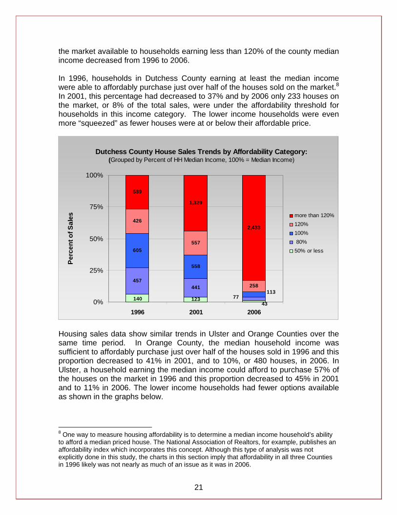
21

the market available to households earning less than 120% of the county median income decreased from 1996 to 2006. In 1996, households in Dutchess County earning at least the median income were able to affordably purchase just over half of the houses sold on the market.8 In 2001, this percentage had decreased to 37% and by 2006 only 233 houses on the market, or 8% of the total sales, were under the affordability threshold for households in this income category. The lower income households were even more “squeezed” as fewer houses were at or below their affordable price.

Dutchess County House Sales Trends by Affordability Category: (Grouped by Percent of HH Median Income, 100% = Median Income)

123

457441

605

558

426

557

258

589

1,329

2,433

43140 77

113

0%

25%

50%

75%

100%

1996 2001 2006

Perc

ent o

f Sal

es

more than 120%120%100% 80%50% or less

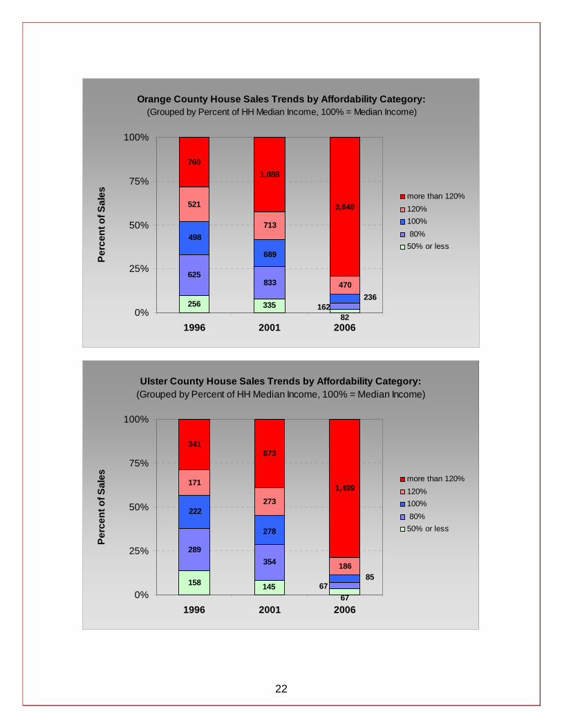
Housing sales data show similar trends in Ulster and Orange Counties over the same time period. In Orange County, the median household income was sufficient to affordably purchase just over half of the houses sold in 1996 and this proportion decreased to 41% in 2001, and to 10%, or 480 houses, in 2006. In Ulster, a household earning the median income could afford to purchase 57% of the houses on the market in 1996 and this proportion decreased to 45% in 2001 and to 11% in 2006. The lower income households had fewer options available as shown in the graphs below.

8 One way to measure housing affordability is to determine a median income household’s ability to afford a median priced house. The National Association of Realtors, for example, publishes an affordability index which incorporates this concept. Although this type of analysis was not explicitly done in this study, the charts in this section imply that affordability in all three Counties in 1996 likely was not nearly as much of an issue as it was in 2006.

22

Orange County House Sales Trends by Affordability Category:(Grouped by Percent of HH Median Income, 100% = Median Income)

256

625833

521

470

1,888

3,649

82335 162

689

498

236

713

760

0%

25%

50%

75%

100%

1996 2001 2006

Perc

ent o

f Sal

es more than 120%120%100% 80%50% or less

Ulster County House Sales Trends by Affordability Category:(Grouped by Percent of HH Median Income, 100% = Median Income)

158

289354

171

186

673

1,499

14567

6785

222

278

273

341

0%

25%

50%

75%

100%

1996 2001 2006

Perc

ent o

f Sal

es more than 120%120%100% 80%50% or less

23

The charts above illustrate how affordability pressures have increased since 1996 and options in the housing market for low- and middle-income households have become fewer and fewer. With fewer affordable options for low- and middle-income households, the low interest rates and a variety of riskier lending products (that included temporary low rates that would reset to higher rates) were attractive and made home ownership achievable and feasible. Still, many of these households found themselves burdened by high housing costs.

24

5. Economic and Demographic Forecasts, 2006 to 2020 Economic conditions, population growth, and household formation will determine housing demand in the 3-County region over the forecast period. This section provides a summary description of the forecast for the relevant economic and demographic variables. A summary is presented for the region overall, and then for each county in the near term (to 2010) and long-term (to 2020). The detailed economic and demographic forecast tables are available in Appendix B on page 54.

5.1 Economic Variables 5.1.1. 3-County Region Summary Overall, the region’s output, or GRP, will increase by 1.5% annually, from $26.8 billion in 2006 to $28.5 billion in 2010.9 Output will then increase by 2% per year out to 2020, to a total of $34.7 billion. It is expected that annual growth will be subdued in the near-term to 2010 and will pick up in the long term out to 2020. This is a result of the current housing market and financial market problems, which are expected to slow growth over the next 2-3 years, nationally and in the 3-County region. Total non-farm employment in the 3-County region will grow from 320,360 in 2006 to 329,420 in 2010, an annual growth of 0.7% over the four year period. Continuing out to 2020, employment will grow slightly faster at about 0.8% per year, reaching 355,480 jobs. The construction and manufacturing sectors are expected to lose 320 jobs and 670 jobs respectively. The total increase in jobs will be 35,480 and most of the growth will come from the education and health services, leisure and hospitality, and financial activities sectors, with 14,910, 5,790, and 3,460 jobs respectively. Growth will be restrained in the near-term due to two primary reasons relating to the housing market: (1) less money will be available for financing mortgages; and (2) and securing that available financing will be difficult due to stricter lending standards and higher down payments likely to be required. This situation presents substantial downside potential as the housing industry is such an important part of the U.S. economy. The inputs that go into building, maintaining and furnishing homes create demand for many other sectors; construction, manufacturing, retail, and the transportation sector are all highly linked to the housing industry. A downturn in the housing market has the potential to cause a ripple effect and spread to other sectors, which has indeed happened in 2008.

9 GRP, or Gross Regional Output, is reported here, and in the individual county sections, in 2000 dollars, adjusted for inflation.

25

Problems in the housing market have spread to the financial sector, which has experienced a “credit crunch” since August of 2007. Banks are wary to lend to each other and investors are skeptical about putting their money into housing linked investments. This drying up of credit translates into less money available for firms to hire new workers and purchase new equipment, and less money available to consumers to make purchases on credit – especially big-ticket items such as cars and homes that typically require financing. In December of 2008, the National Bureau of Economic Research (NBER) announced that the United States entered into a recession in December of 2007. The announcement confirmed what virtually all economic indicators had been suggesting most of the year. Home prices and sales, retail sales, and employment levels have all fallen and the unemployment rate has risen. While output in the first and second quarters of the year technically remained positive, inventories grew while domestic consumption actually went negative, an indication that there probably was no real growth in the output of the economy. Data for the third and fourth quarter confirm that the national economy did indeed contract, as was expected by analysts. The recovery from this downturn is expected to be at a historically slow pace and take at least the next 2-3 years, and possibly longer without significant and on-going intervention through fiscal (e.g. the 2nd stimulus package currently being debated) and monetary policy. The following sections present the forecast for each County. 5.1.2. Dutchess County The forecast shows that in Dutchess County, GRP is expected to increase from $10.3 billion in 2006 to $10.9 billion in 2010, an increase of 1.5% per year (GRP is in 2000 dollars, adjusted for inflation). GRP is then expected to grow by about 1.7% per year to $12.9 billion in 2020. Total non-farm employment in the county will grow from 121,820 in 2006 to 123,220 in 2010. This is an increase of 1,400 jobs or 0.3% per year. Non-farm employment is expected to then grow by 0.4% per year until 2020, when 6,680 jobs will have been added to 2006 employment levels. The NAICS10 sectors that are expected to lose jobs include construction, manufacturing, trade-transportation-utilities, and government employment. Financial activities, education and health services, and leisure and hospitality are sectors expected to add jobs. Most of the net increase in jobs will come from the education and health services sector, representing 5,300 of the 6,680 new jobs in the county. The sectors to be hardest hit will be manufacturing and trade-transportation-utilities, which are expected to lose 810 and 720 jobs respectively, by 2020. 5.1.3. Orange County Orange County’s GRP is expected to increase from $11.4 billion in 2006 to $12.2 billion in 2010, an increase of 1.7% over the four year period. From 2010 to 10 NAICS stands for North American Industrial Classification System, a standard government system to classify industries.

26

2020, GRP will grow by 2.4% per year to $15.4 billion. The employment forecast for Orange County shows solid growth over the forecast period. Non-farm employment will increase from 133,730 jobs in 2006 to 138,800 jobs in 2010, an increase of 0.9% per year. Growth will then continue at about 1% per year until 2020, when non-farm employment is expected to reach 153,910 jobs, an increase of 20,200 jobs. The only major NAICS sector expected to see a decline in jobs is construction (and this decline is minor – only 40 jobs), while manufacturing, trade-transportation-utilities, financial activities, education and health services, leisure and hospitality, and government employment are all expected to grow. Most of the additional jobs will be in the education and health services sector, which will add about 6,910 jobs, followed by trade-transportation-utilities and government employment, which are expected to grow by about 2,730 and 2,107 jobs respectively. 5.1.4. Ulster County GRP of Ulster County is expected to grow at a yearly compounded rate of 1.2% from $5.1 billion in 2006 to $5.4 billion in 2010. Growth in GRP out to 2020 will be at about 1.8% per year and GRP will reach $6.4 billion. Total non-farm employment in Ulster County will increase from 64,810 in 2006 to 67,390 in 2010, an increase of 0.9% per year. Continuing the forecast out to 2020, total non-farm employment will continue to grow at an annual rate of 0.8% per year to 73,070 jobs. The manufacturing sector is expected to lose about 170 jobs, and government employment will decrease by about 270 jobs. The construction, trade-transportation-utilities, financial activities, education and health services, and leisure and hospitality sectors will add jobs. Most of the 8,260 additional jobs will be in the education and health services and leisure and hospitality sectors, with each adding 2,700 and 2,600 jobs respectively. Financial activities will grow by 900 jobs and trade-transportation-utilities will grow by 860 jobs.

5.2 Demographic Variables 5.2.1. 3-County Region Summary The population of the 3-County region overall will grow from 855,920 in 2006 to 872,340 in 2010, an increase of 16,420, or annual growth of 0.5%. Growth will continue at about the same annual rate of 0.5% out to 2020 and 48,020 more residents will be added to the population bringing the total to 920,360. Most of the growth will be among older residents: of the total increase of 64,440 persons over the period 2006 to 2020, more than 40,000 will come from the 65 and over age group, and more than 19,000 will come from the age group 45 to 64. The number of households in the region will grow by 0.7% per year, adding 8,500 new households by 2010. Household growth will continue at the rate of more than 0.8% per year going forward to 2020, and 28,300 more households will be added. Given the trend of declining household size described above for each county, the average household size for the region overall will also decline from 2.84 persons per household in 2006 to 2.81 in 2010, and to 2.72 in 2020.

27

5.2.2 Dutchess County The population of Dutchess County is expected to grow from 295,140 in 2006 to 297,570 in 2010. This is an increase of 2,430 persons, or annual growth of 0.2%. Average annual growth will increase to 0.4% per year through 2020, adding 14,260 additional residents and bringing the total population to 311,830 persons. According to the population projections, the age group 65 and over will make the largest contribution to overall population growth from 2006 to 2020, followed by the age group 45 to 64. The other age groups will actually experience declines in population, with the exception of the 0 to 4 age group, which will grow, although at a weak rate of growth. The number of households in the county will increase by about 0.3% per year to 2010, adding 1,300 new households, and then by more than 0.8% per year to 2020, adding 10,000 more households. The fact that households are expected to grow at a faster rate than population reflects the trend in declining household size, a result of both an aging population and declining family size. In Dutchess County, households, on average consisted of 2.81 persons per household in 2006, and this will remain roughly unchanged at 2.80 in 2010 and decrease to 2.68 persons per household by 2020. 5.2.3. Orange County Orange County will add 10,830 residents, growing from 376,400 in 2006 to 387,230 in 2010, an annual growth rate of 0.7%. The rate of growth will decrease slightly to about 0.6% per year out to 2020. This will add 23,840 residents and bring the total population to 411,070. The age group contributing most to the overall growth will be the 65 and over group, followed by 45 to 64 and 25-44 age groups. Households in Orange County will increase by about 1.0% per year to 2010 adding 5,100 households, and continue growth at 1.0% per year and add 13,700 more households by 2020. The population and household growth rates in Orange County also indicate that average household size will decrease over the forecast period. Average persons per household stood at 2.97 in 2006 this figure is projected to decrease to 2.94 in 2010, and then to 2.83 in 2020. 5.2.4. Ulster County Ulster County’s population will grow from 184,390 in 2006 to 187,530 in 2010, an increase of 3,140 residents at an annual growth rate of 0.3% per year. Growth will continue to 2020 at a rate of 0.5% per year, adding 9,930 residents and bring the total population to 197,460. The largest contributions to the overall population growth will be from the 45 to 64 age group followed by the 65 and over and 25 to 44 age groups. The county will add 1,900 households by 2010, growing at an annual rate of 0.6%, and then continue growth at a similar annual rate and add 4,500 more

28

households by 2020. Average household size will decline from 2.63 persons per household in 2006 to 2.61 in 2010, reaching 2.58 in 2020.

29

6. Current Housing Units Needed, 2006

6.1 Affordability Gap Analysis This section provides estimates of the need for additional housing units in the 3-County region in 2006.11 Need was determined using a “gap” analysis in which supply and demand were estimated and then compared against each other. This was done by income category and by tenure status (owner and renter households). An inventory update as of December 31, 2006 was made and this represents the supply side of the ledger. Demand by income and tenure status was estimated based on available data sources and the two are compared – demand versus supply. Such a comparison reveals whether or not demand exceeds supply, and if so to what extent, at each household income level and for owners and renters. If demand exceeds supply, such a gap is an indication that the number of units available to be purchased (or rented for the renter part of the analysis) at an affordable price (or rent) is not sufficient, and households will likely be paying more than the HUD threshold of 30% of household income toward housing costs. The gap analysis incorporated the affordability calculations described in Section 2 above. The affordable house prices and rents were determined by income category relative to the County median household income: 50%, 80%, 100%, and 120% of median household income. Estimates of the number of owner and renter units demanded were based on distributions of household income reported from the 2006 American Community Survey. Estimates of unit supply were developed based on a variety of sources, including the 2006 American Community Survey unit data, building permit data, respective County Planning Department rental surveys, and parcel data used for property tax purposes. The analysis confirmed that there are current affordability gaps in each of the 3 counties. Owner unit demand exceeds supply for all income categories at or below 120% of the County median household income. In Dutchess County, there is a 6,664 unit gap at 50% of median household income level, a 7,556 unit gap at 80% of median household income, a 3,225 unit gap at the median household income, and a 468 unit gap at 120% of the median household income. In Orange County, there is a 9,528 unit gap at 50% of median household income level, a 5,753 unit gap at 80% of median household income, a 5,312 unit gap at the median household income, and a 1,328 unit gap at 120% of the median household income. In Ulster County, there is a 5,936 unit gap at 50% of median household income level, a 2,746 unit gap at 80% of median household income, a 1,216 unit gap at the median household income, and a 798 unit gap at 120% of the median household income. For the 3-County region overall, these figures sum to a 22,129 unit gap at 50% of median household income level, a 16,055 11 The inventory update is made for 2006, the base year of the study and the jumping off point for the forecasts.

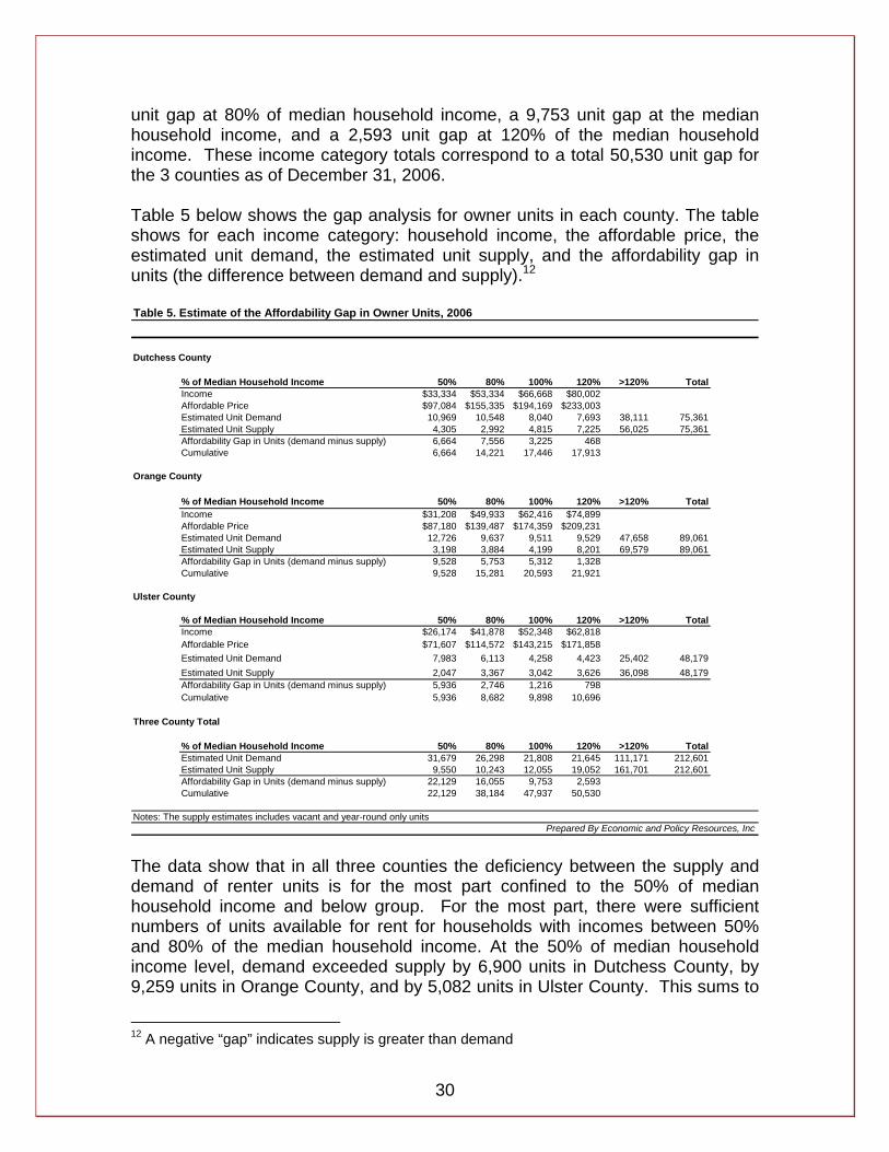
30

unit gap at 80% of median household income, a 9,753 unit gap at the median household income, and a 2,593 unit gap at 120% of the median household income. These income category totals correspond to a total 50,530 unit gap for the 3 counties as of December 31, 2006. Table 5 below shows the gap analysis for owner units in each county. The table shows for each income category: household income, the affordable price, the estimated unit demand, the estimated unit supply, and the affordability gap in units (the difference between demand and supply).12 Table 5. Estimate of the Affordability Gap in Owner Units, 2006

Dutchess County

% of Median Household Income 50% 80% 100% 120% >120% TotalIncome $33,334 $53,334 $66,668 $80,002Affordable Price $97,084 $155,335 $194,169 $233,003Estimated Unit Demand 10,969 10,548 8,040 7,693 38,111 75,361Estimated Unit Supply 4,305 2,992 4,815 7,225 56,025 75,361Affordability Gap in Units (demand minus supply) 6,664 7,556 3,225 468 -17,913Cumulative 6,664 14,221 17,446 17,913

Orange County

% of Median Household Income 50% 80% 100% 120% >120% TotalIncome $31,208 $49,933 $62,416 $74,899Affordable Price $87,180 $139,487 $174,359 $209,231Estimated Unit Demand 12,726 9,637 9,511 9,529 47,658 89,061Estimated Unit Supply 3,198 3,884 4,199 8,201 69,579 89,061Affordability Gap in Units (demand minus supply) 9,528 5,753 5,312 1,328 -21,921Cumulative 9,528 15,281 20,593 21,921

Ulster County

% of Median Household Income 50% 80% 100% 120% >120% TotalIncome $26,174 $41,878 $52,348 $62,818Affordable Price $71,607 $114,572 $143,215 $171,858Estimated Unit Demand 7,983 6,113 4,258 4,423 25,402 48,179Estimated Unit Supply 2,047 3,367 3,042 3,626 36,098 48,179Affordability Gap in Units (demand minus supply) 5,936 2,746 1,216 798 -10,696Cumulative 5,936 8,682 9,898 10,696

Three County Total

% of Median Household Income 50% 80% 100% 120% >120% TotalEstimated Unit Demand 31,679 26,298 21,808 21,645 111,171 212,601Estimated Unit Supply 9,550 10,243 12,055 19,052 161,701 212,601Affordability Gap in Units (demand minus supply) 22,129 16,055 9,753 2,593 -50,530Cumulative 22,129 38,184 47,937 50,530

Notes: The supply estimates includes vacant and year-round only unitsPrepared By Economic and Policy Resources, Inc

The data show that in all three counties the deficiency between the supply and demand of renter units is for the most part confined to the 50% of median household income and below group. For the most part, there were sufficient numbers of units available for rent for households with incomes between 50% and 80% of the median household income. At the 50% of median household income level, demand exceeded supply by 6,900 units in Dutchess County, by 9,259 units in Orange County, and by 5,082 units in Ulster County. This sums to

12 A negative “gap” indicates supply is greater than demand

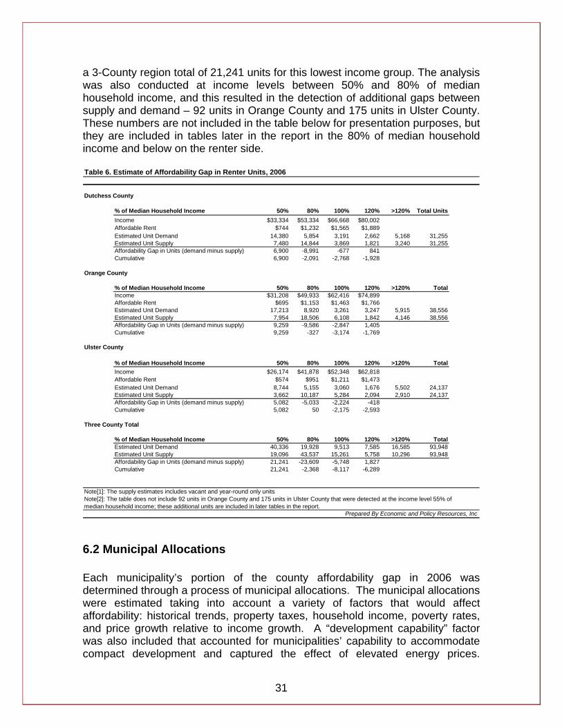
31

a 3-County region total of 21,241 units for this lowest income group. The analysis was also conducted at income levels between 50% and 80% of median household income, and this resulted in the detection of additional gaps between supply and demand – 92 units in Orange County and 175 units in Ulster County. These numbers are not included in the table below for presentation purposes, but they are included in tables later in the report in the 80% of median household income and below on the renter side. Table 6. Estimate of Affordability Gap in Renter Units, 2006

Dutchess County

% of Median Household Income 50% 80% 100% 120% >120% Total UnitsIncome $33,334 $53,334 $66,668 $80,002Affordable Rent $744 $1,232 $1,565 $1,889Estimated Unit Demand 14,380 5,854 3,191 2,662 5,168 31,255Estimated Unit Supply 7,480 14,844 3,869 1,821 3,240 31,255Affordability Gap in Units (demand minus supply) 6,900 -8,991 -677 841 1,928Cumulative 6,900 -2,091 -2,768 -1,928

Orange County

% of Median Household Income 50% 80% 100% 120% >120% TotalIncome $31,208 $49,933 $62,416 $74,899Affordable Rent $695 $1,153 $1,463 $1,766Estimated Unit Demand 17,213 8,920 3,261 3,247 5,915 38,556Estimated Unit Supply 7,954 18,506 6,108 1,842 4,146 38,556Affordability Gap in Units (demand minus supply) 9,259 -9,586 -2,847 1,405 1,769Cumulative 9,259 -327 -3,174 -1,769

Ulster County

% of Median Household Income 50% 80% 100% 120% >120% TotalIncome $26,174 $41,878 $52,348 $62,818Affordable Rent $574 $951 $1,211 $1,473Estimated Unit Demand 8,744 5,155 3,060 1,676 5,502 24,137Estimated Unit Supply 3,662 10,187 5,284 2,094 2,910 24,137Affordability Gap in Units (demand minus supply) 5,082 -5,033 -2,224 -418 2,593Cumulative 5,082 50 -2,175 -2,593

Three County Total

% of Median Household Income 50% 80% 100% 120% >120% TotalEstimated Unit Demand 40,336 19,928 9,513 7,585 16,585 93,948Estimated Unit Supply 19,096 43,537 15,261 5,758 10,296 93,948Affordability Gap in Units (demand minus supply) 21,241 -23,609 -5,748 1,827 6,289Cumulative 21,241 -2,368 -8,117 -6,289

Note[1]: The supply estimates includes vacant and year-round only unitsNote[2]: The table does not include 92 units in Orange County and 175 units in Ulster County that were detected at the income level 55% ofmedian household income; these additional units are included in later tables in the report.

Prepared By Economic and Policy Resources, Inc

6.2 Municipal Allocations Each municipality’s portion of the county affordability gap in 2006 was determined through a process of municipal allocations. The municipal allocations were estimated taking into account a variety of factors that would affect affordability: historical trends, property taxes, household income, poverty rates, and price growth relative to income growth. A “development capability” factor was also included that accounted for municipalities’ capability to accommodate compact development and captured the effect of elevated energy prices.

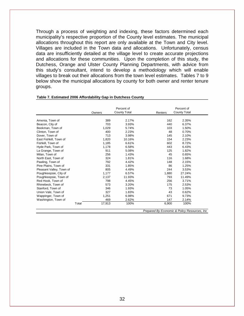
32

Through a process of weighting and indexing, these factors determined each municipality’s respective proportion of the County level estimates. The municipal allocations throughout this report are only available at the Town and City level. Villages are included in the Town data and allocations. Unfortunately, census data are insufficiently detailed at the village level to create accurate projections and allocations for these communities. Upon the completion of this study, the Dutchess, Orange and Ulster County Planning Departments, with advice from this study’s consultant, intend to develop a methodology which will enable villages to break out their allocations from the town level estimates. Tables 7 to 9 below show the municipal allocations by county for both owner and renter tenure groups. Table 7. Estimated 2006 Affordability Gap in Dutchess County

OwnersPercent of

County Total RentersPercent of

County Total

Amenia, Town of 389 2.17% 162 2.35%Beacon, City of 703 3.93% 440 6.37%Beekman, Town of 1,029 5.74% 103 1.50%Clinton, Town of 400 2.23% 48 0.70%Dover, Town of 713 3.98% 145 2.10%East Fishkill, Town of 1,820 10.16% 154 2.23%Fishkill, Town of 1,185 6.61% 602 8.72%Hyde Park, Town of 1,178 6.58% 443 6.43%La Grange, Town of 911 5.08% 125 1.82%Milan, Town of 256 1.43% 45 0.65%North East, Town of 324 1.81% 116 1.68%Pawling, Town of 792 4.42% 148 2.15%Pine Plains, Town of 331 1.85% 86 1.25%Pleasant Valley, Town of 805 4.49% 244 3.53%Poughkeepsie, City of 1,177 6.57% 1,880 27.24%Poughkeepsie, Town of 2,137 11.93% 793 11.49%Red Hook, Town of 798 4.45% 256 3.71%Rhinebeck, Town of 573 3.20% 175 2.53%Stanford, Town of 346 1.93% 73 1.05%Union Vale, Town of 327 1.83% 43 0.62%Wappinger, Town of 1,251 6.98% 671 9.73%Washington, Town of 469 2.62% 147 2.14%

Total 17,913 100% 6,900 100%


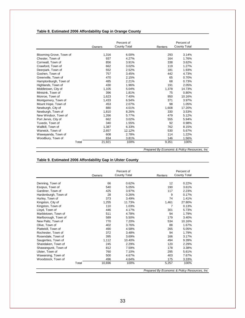
33

Table 8. Estimated 2006 Affordability Gap in Orange County

OwnersPercent of


County Total

Blooming Grove, Town of 1,316 6.00% 293 3.14%Chester, Town of 937 4.27% 164 1.76%Cornwall, Town of 856 3.91% 338 3.62%Crawford, Town of 662 3.02% 119 1.27%Deerpark, Town of 552 2.52% 181 1.93%Goshen, Town of 757 3.45% 442 4.73%Greenville, Town of 470 2.15% 65 0.70%Hamptonburgh, Town of 485 2.21% 68 0.73%Highlands, Town of 430 1.96% 191 2.05%Middletown, City of 1,105 5.04% 1,378 14.73%Minisink, Town of 396 1.81% 75 0.80%Monroe, Town of 1,623 7.40% 950 10.16%Montgomery, Town of 1,433 6.54% 371 3.97%Mount Hope, Town of 453 2.07% 98 1.05%Newburgh, City of 880 4.01% 1,608 17.20%Newburgh, Town of 1,810 8.26% 330 3.53%New Windsor, Town of 1,266 5.77% 479 5.12%Port Jervis, City of 662 3.02% 555 5.94%Tuxedo, Town of 340 1.55% 92 0.98%Wallkill, Town of 1,387 6.33% 762 8.15%Warwick, Town of 2,657 12.12% 530 5.67%Wawayanda, Town of 608 2.78% 114 1.22%Woodbury, Town of 834 3.81% 146 1.56%

Total 21,921 100% 9,351 100%

Prepared By Economic & Policy Resources, Inc Table 9. Estimated 2006 Affordability Gap in Ulster County

OwnersPercent of


County Total

Denning, Town of 66 0.62% 12 0.22%Esopus, Town of 540 5.05% 190 3.61%Gardiner, Town of 425 3.97% 117 2.23%Hardenburgh, Town of 28 0.26% 9 0.17%Hurley, Town of 373 3.49% 74 1.41%Kingston, City of 1,255 11.73% 1,461 27.80%Kingston, Town of 110 1.03% 7 0.13%Lloyd, Town of 446 4.17% 301 5.73%Marbletown, Town of 511 4.78% 94 1.79%Marlborough, Town of 589 5.50% 179 3.40%New Paltz, Town of 770 7.20% 534 10.16%Olive, Town of 402 3.76% 88 1.67%Plattekill, Town of 490 4.58% 265 5.05%Rochester, Town of 372 3.48% 94 1.79%Rosendale, Town of 395 3.69% 166 3.17%Saugerties, Town of 1,112 10.40% 494 9.39%Shandaken, Town of 245 2.29% 120 2.29%Shawangunk, Town of 812 7.59% 178 3.38%Ulster, Town of 760 7.10% 295 5.61%Wawarsing, Town of 500 4.67% 403 7.67%Woodstock, Town of 496 4.64% 175 3.33%

Total 10,696 100% 5,257 100%


34

7. Prospective Housing Units Needed, 2006 to 2020 The estimates of the municipal allocations were then projected out to the year 2020, the forecast horizon of the RHNA. The projections were made based on historical trends and the “development capability” factor described above, which reflects the expectation that future housing unit demand and affordability challenges will be concentrated in those communities with sufficient infrastructure to accommodate compact development. In today’s planning language, these allocations are a balance between a traditional “fair-share” approach where units are allocated based on the existing housing stock and a “smart growth” approach where units are focused around existing centers and infrastructure. The core of these allocations is a “fair share approach” with modest adjustments for “smart growth” criteria. The tables 10 to 15 below show the projections of the affordability gaps out to 2020. The tables also include total unit demand (or total expected units in other words) out to 2020. For owner and renter units in Dutchess County, affordability pressures and additional total demand for units are expected to be concentrated in Beacon City, the Town of Fishkill, the City of Poughkeepsie, the Town of Poughkeepsie, and the Town of Wappinger. These municipalities were designated as those areas that are already compact and most capable of compact development in the future. To a lesser extent, growth is also expected in Amenia, Dover, East Fishkill, Hyde Park, LaGrange, Pawling, Pleasant Valley, Red Hook and Rhinebeck, the municipalities designated as capable of some compact development. In Orange County, substantial affordability pressures and additional total unit demand for both owner and renter units are expected to be concentrated primarily in the Cities of Middletown and Newburgh, and the Towns of Monroe, Montgomery, Newburgh, New Windsor, and Wallkill, and Warwick – the municipalities designated as already compact or highly capable of compact development in the future. Communities designated as capable of compact future development were the Town of Blooming Grove, the Town of Chester, the Town of Goshen, the Town of Montgomery, the City of Port Jervis, the Town of Warwick, and the Town of Wawayanda. Additional demand is also expected in these municipalities and affordability pressures will increase over the forecast horizon. In Ulster County, the City of Kingston and the Town of Ulster were designated as municipalities that are already compact and highly capable of future compact development. Growth in total unit demand and increasing affordability pressures are expected to occur in these two communities, and to a lesser extent in the Towns of Lloyd, Marlborough, New Paltz, Saugerties, Shawangunk, and Wawarsing.

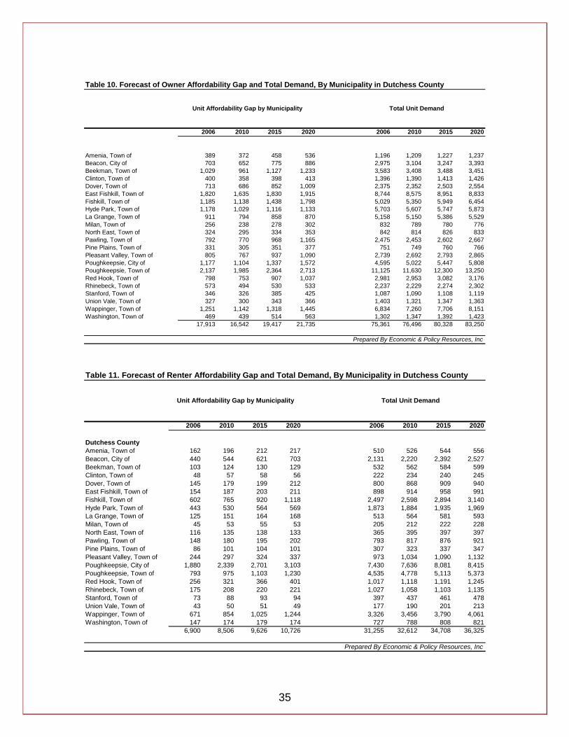
35

Table 10. Forecast of Owner Affordability Gap and Total Demand, By Municipality in Dutchess County

2006 2010 2015 2020 2006 2010 2015 2020

Amenia, Town of 389 372 458 536 1,196 1,209 1,227 1,237Beacon, City of 703 652 775 886 2,975 3,104 3,247 3,393Beekman, Town of 1,029 961 1,127 1,233 3,583 3,408 3,488 3,451Clinton, Town of 400 358 398 413 1,396 1,390 1,413 1,426Dover, Town of 713 686 852 1,009 2,375 2,352 2,503 2,554East Fishkill, Town of 1,820 1,635 1,830 1,915 8,744 8,575 8,951 8,833Fishkill, Town of 1,185 1,138 1,438 1,798 5,029 5,350 5,949 6,454Hyde Park, Town of 1,178 1,029 1,116 1,133 5,703 5,607 5,747 5,873La Grange, Town of 911 794 858 870 5,158 5,150 5,386 5,529Milan, Town of 256 238 278 302 832 789 780 776North East, Town of 324 295 334 353 842 814 826 833Pawling, Town of 792 770 968 1,165 2,475 2,453 2,602 2,667Pine Plains, Town of 331 305 351 377 751 749 760 766Pleasant Valley, Town of 805 767 937 1,090 2,739 2,692 2,793 2,865Poughkeepsie, City of 1,177 1,104 1,337 1,572 4,595 5,022 5,447 5,808Poughkeepsie, Town of 2,137 1,985 2,364 2,713 11,125 11,630 12,300 13,250Red Hook, Town of 798 753 907 1,037 2,981 2,953 3,082 3,176Rhinebeck, Town of 573 494 530 533 2,237 2,229 2,274 2,302Stanford, Town of 346 326 385 425 1,087 1,090 1,108 1,119Union Vale, Town of 327 300 343 366 1,403 1,321 1,347 1,363Wappinger, Town of 1,251 1,142 1,318 1,445 6,834 7,260 7,706 8,151Washington, Town of 469 439 514 563 1,302 1,347 1,392 1,423

17,913 16,542 19,417 21,735 75,361 76,496 80,328 83,250


Unit Affordability Gap by Municipality Total Unit Demand

Table 11. Forecast of Renter Affordability Gap and Total Demand, By Municipality in Dutchess County

2006 2010 2015 2020 2006 2010 2015 2020

Dutchess CountyAmenia, Town of 162 196 212 217 510 526 544 556Beacon, City of 440 544 621 703 2,131 2,220 2,392 2,527Beekman, Town of 103 124 130 129 532 562 584 599Clinton, Town of 48 57 58 56 222 234 240 245Dover, Town of 145 179 199 212 800 868 909 940East Fishkill, Town of 154 187 203 211 898 914 958 991Fishkill, Town of 602 765 920 1,118 2,497 2,598 2,894 3,140Hyde Park, Town of 443 530 564 569 1,873 1,884 1,935 1,969La Grange, Town of 125 151 164 168 513 564 581 593Milan, Town of 45 53 55 53 205 212 222 228North East, Town of 116 135 138 133 365 395 397 397Pawling, Town of 148 180 195 202 793 817 876 921Pine Plains, Town of 86 101 104 101 307 323 337 347Pleasant Valley, Town of 244 297 324 337 973 1,034 1,090 1,132Poughkeepsie, City of 1,880 2,339 2,701 3,103 7,430 7,636 8,081 8,415Poughkeepsie, Town of 793 975 1,103 1,230 4,535 4,778 5,113 5,373Red Hook, Town of 256 321 366 401 1,017 1,118 1,191 1,245Rhinebeck, Town of 175 208 220 221 1,027 1,058 1,103 1,135Stanford, Town of 73 88 93 94 397 437 461 478Union Vale, Town of 43 50 51 49 177 190 201 213Wappinger, Town of 671 854 1,025 1,244 3,326 3,456 3,790 4,061Washington, Town of 147 174 179 174 727 788 808 821

6,900 8,506 9,626 10,726 31,255 32,612 34,708 36,325



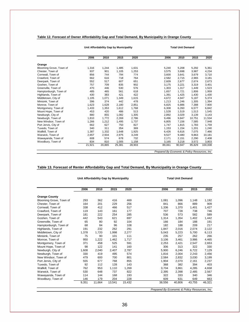
36

Table 12. Forecast of Owner Affordability Gap and Total Demand, By Municipality in Orange County

2006 2010 2015 2020 2006 2010 2015 2020

OrangeBlooming Grove, Town of 1,316 1,244 1,485 1,631 5,240 5,208 5,292 5,361Chester, Town of 937 901 1,105 1,253 3,575 3,698 3,987 4,234Cornwall, Town of 856 744 794 774 3,600 3,641 3,679 3,710Crawford, Town of 662 616 718 764 2,582 2,715 2,965 3,181Deerpark, Town of 552 517 607 651 2,609 2,677 2,674 2,673Goshen, Town of 757 709 835 902 3,175 3,221 3,319 3,401Greenville, Town of 470 446 530 576 1,303 1,317 1,449 1,523Hamptonburgh, Town of 485 465 561 618 1,657 1,721 1,806 1,959Highlands, Town of 430 383 421 422 1,391 1,425 1,430 1,430Middletown, City of 1,105 1,071 1,349 1,615 4,672 4,947 5,187 5,374Minisink, Town of 396 374 442 478 1,213 1,246 1,305 1,394Monroe, Town of 1,623 1,628 2,180 2,851 6,825 6,886 7,388 7,900Montgomery, Town of 1,433 1,353 1,612 1,768 6,308 6,260 6,577 6,842Mount Hope, Town of 453 420 486 513 1,528 1,519 1,513 1,545Newburgh, City of 880 855 1,082 1,305 2,892 3,029 3,139 3,143Newburgh, Town of 1,810 1,772 2,269 2,786 9,496 9,847 10,751 11,534New Windsor, Town of 1,266 1,212 1,495 1,737 6,805 7,156 7,585 7,948Port Jervis, City of 662 627 750 827 1,747 1,815 1,783 1,759Tuxedo, Town of 340 311 354 369 1,153 1,154 1,201 1,240Wallkill, Town of 1,387 1,332 1,648 1,925 6,426 6,616 7,075 7,466Warwick, Town of 2,657 2,504 2,975 3,249 9,527 9,480 9,863 10,181Wawayanda, Town of 608 574 678 732 2,171 2,151 2,290 2,408Woodbury, Town of 834 810 1,005 1,158 3,165 3,218 3,572 3,803

21,921 20,865 25,381 28,903 89,061 90,947 95,829 100,008



Table 13. Forecast of Renter Affordability Gap and Total Demand, By Municipality in Orange County

2006 2010 2015 2020 2006 2010 2015 2020

Orange CountyBlooming Grove, Town of 293 362 416 469 1,081 1,096 1,148 1,192Chester, Town of 164 201 229 256 841 866 889 909Cornwall, Town of 338 412 466 517 1,336 1,370 1,401 1,427Crawford, Town of 119 143 161 177 707 728 738 746Deerpark, Town of 181 222 254 285 536 573 582 589Goshen, Town of 442 543 621 697 1,314 1,354 1,402 1,442Greenville, Town of 65 80 92 104 166 184 188 191Hamptonburgh, Town of 68 84 96 108 182 188 209 217Highlands, Town of 191 232 262 291 1,847 2,016 2,074 2,122Middletown, City of 1,378 1,720 1,998 2,277 5,043 5,223 5,700 6,113Minisink, Town of 75 90 101 111 235 257 262 266Monroe, Town of 950 1,222 1,462 1,717 3,106 3,461 3,986 4,465Montgomery, Town of 371 458 525 591 2,253 2,421 2,547 2,653Mount Hope, Town of 98 122 141 160 306 313 322 330Newburgh, City of 1,608 2,040 2,407 2,787 5,900 6,246 6,722 7,129Newburgh, Town of 330 419 495 574 1,816 2,004 2,243 2,456New Windsor, Town of 479 600 700 801 2,584 2,832 3,030 3,199Port Jervis, City of 555 677 768 855 1,904 2,070 2,161 2,237Tuxedo, Town of 92 112 128 143 368 382 394 403Wallkill, Town of 762 953 1,110 1,269 3,704 3,861 4,285 4,658Warwick, Town of 530 648 737 822 2,395 2,398 2,485 2,567Wawayanda, Town of 114 144 168 193 322 333 340 346Woodbury, Town of 146 179 204 228 609 631 649 663

9,351 11,664 13,541 15,432 38,556 40,806 43,755 46,321



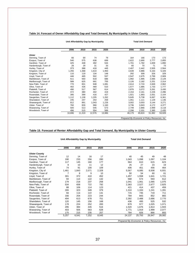
37

Table 14. Forecast of Owner Affordability Gap and Total Demand, By Municipality in Ulster County

2006 2010 2015 2020 2006 2010 2015 2020

Ulster Denning, Town of 66 69 74 79 164 166 170 173Esopus, Town of 540 575 638 699 2,622 2,690 2,777 2,855Gardiner, Town of 425 448 492 534 1,701 1,782 1,839 1,890Hardenburgh, Town of 28 29 31 33 65 70 71 73Hurley, Town of 373 388 418 445 2,407 2,442 2,505 2,564Kingston, City of 1,255 1,368 1,610 1,950 4,639 4,886 5,164 5,426Kingston, Town of 110 119 134 148 292 309 326 329Lloyd, Town of 446 465 502 537 2,547 2,675 2,799 2,909Marbletown, Town of 511 550 618 686 1,992 1,995 2,065 2,129Marlborough, Town of 589 625 691 755 2,126 2,182 2,251 2,314New Paltz, Town of 770 831 948 1,081 2,614 2,724 2,849 2,962Olive, Town of 402 426 469 510 1,577 1,685 1,733 1,777Plattekill, Town of 490 517 567 614 2,876 3,072 3,261 3,430Rochester, Town of 372 380 402 419 2,153 2,161 2,226 2,286Rosendale, Town of 395 399 416 427 1,921 1,993 2,051 2,104Saugerties, Town of 1,112 1,138 1,205 1,262 5,645 5,738 6,067 6,361Shandaken, Town of 245 247 254 259 1,051 1,111 1,129 1,146Shawangunk, Town of 812 891 1,043 1,226 3,002 3,003 3,144 3,271Ulster, Town of 760 826 966 1,160 3,736 3,943 4,172 4,377Wawarsing, Town of 500 513 545 573 2,749 2,866 2,999 3,118Woodstock, Town of 496 515 554 589 2,298 2,331 2,385 2,435

10,696 11,319 12,576 13,986 48,179 49,824 51,982 53,928



Table 15. Forecast of Renter Affordability Gap and Total Demand, By Municipality in Ulster County

2006 2010 2015 2020 2006 2010 2015 2020

Ulster CountyDenning, Town of 12 14 16 17 40 45 49 48Esopus, Town of 190 233 256 280 1,043 1,098 1,097 1,104Gardiner, Town of 117 145 160 177 564 610 615 623Hardenburgh, Town of 9 10 11 12 25 27 23 19Hurley, Town of 74 91 100 109 406 451 456 464Kingston, City of 1,461 1,843 2,071 2,328 5,567 6,085 6,508 6,931Kingston, Town of 7 8 9 10 50 54 60 61Lloyd, Town of 301 372 410 452 1,457 1,558 1,641 1,721Marbletown, Town of 94 114 122 132 568 574 593 612Marlborough, Town of 179 218 237 258 1,041 1,061 1,065 1,075New Paltz, Town of 534 658 722 792 2,363 2,527 2,677 2,825Olive, Town of 88 106 114 123 421 414 437 459Plattekill, Town of 265 323 349 379 1,310 1,333 1,241 1,281Rochester, Town of 94 114 122 131 715 735 719 711Rosendale, Town of 166 204 223 244 784 843 852 865Saugerties, Town of 494 613 678 751 2,392 2,488 2,686 2,770Shandaken, Town of 120 145 156 168 436 495 525 532Shawangunk, Town of 178 224 252 283 879 977 1,025 1,071Ulster, Town of 295 384 445 516 1,520 1,676 1,814 1,943Wawarsing, Town of 403 505 563 628 1,771 1,919 1,999 2,077Woodstock, Town of 175 215 235 257 784 826 866 893

5,257 6,541 7,252 8,045 24,137 25,793 26,947 28,082



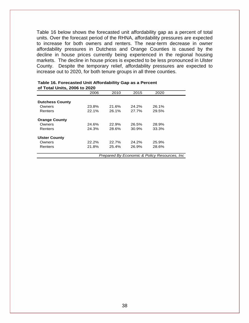
38

Table 16 below shows the forecasted unit affordability gap as a percent of total units. Over the forecast period of the RHNA, affordability pressures are expected to increase for both owners and renters. The near-term decrease in owner affordability pressures in Dutchess and Orange Counties is caused by the decline in house prices currently being experienced in the regional housing markets. The decline in house prices is expected to be less pronounced in Ulster County. Despite the temporary relief, affordability pressures are expected to increase out to 2020, for both tenure groups in all three counties. Table 16. Forecasted Unit Affordability Gap as a Percentof Total Units, 2006 to 2020

2006 2010 2015 2020

Dutchess County Owners 23.8% 21.6% 24.2% 26.1% Renters 22.1% 26.1% 27.7% 29.5%

Orange County Owners 24.6% 22.9% 26.5% 28.9% Renters 24.3% 28.6% 30.9% 33.3%

Ulster County Owners 22.2% 22.7% 24.2% 25.9% Renters 21.8% 25.4% 26.9% 28.6%


39

8. Targets for Building Affordable Housing

8.1 Strategies to Address Affordability Challenges Affordable housing remedies have traditionally been categorized into two approaches: demand side solutions or supply side solutions. A demand side approach would attempt to make housing more affordable from the perspective of the households. The primary instrument of this demand side approach for owners has been through assistance with financing and down payments, usually considered the two most prohibitive barriers to home ownership. For renters, the primary instrument to increase households’ ability to pay has been through subsidizing apartment units with the federal Section 8 housing assistance program. From the supply side perspective, affordable housing can be addressed by increasing the supply of affordable units. This can be done through planning and zoning regulatory changes, or through incentives for developers. The Planning Departments of the three counties agree that this supply side approach is the option over which county and municipality governments in the region can have the most influence, and the avenue through which they can make a substantial impact in their respective areas. Therefore, one of the goals of this RHNA was to establish the quantity of affordable housing units to construct that would help to alleviate the affordability pressures, should the Counties and municipalities decide that such an approach is appropriate. The build targets are presented in two sections, the first focusing on the current affordability gap (as of 2006), and the second focusing on the prospective affordability gap (out to 2020). The current and prospective built targets combined represent the total number of affordable units to construct in order to address both the current and prospective affordability gaps. The building of additional affordable units is not a “magic bullet” solution and this supply side strategy is likely to be effective only when part of broader efforts to remedy the situation, including both demand and supply side initiatives. Solutions to housing affordability challenges usually include other strategic economic development efforts that seek to create and retain jobs in the local economy, as well as increase the incomes earned by residents in the community. While the previous sections described the current and expected need for affordable housing in the 3-County region, the following section provides estimates of how many affordable units the Counties would need to construct in order to meet some of that need. It should be emphasized that constructing additional affordable units would only address a portion of the overall affordability gap.

40

8.2 Build Targets to Address the 2006 Affordability Gap There are different approaches that can be taken regarding how many housing units would be needed in order to address the current affordability challenges. Units can be built to target certain members of the population, either by age or income, and there are logical arguments to support these different supply side strategies. In this RHNA, a build number was calculated that attempts to minimize value judgment and still address the need for affordable housing. The build number was calculated based on the declining household size trend, a demographic trend that many counties in the northeast part of the country have experienced over the last twenty to twenty-five years. The logic behind the calculation is that as the average household size decreases, just this trend alone places additional pressure on the housing stock that must provide sufficient housing units. If the average household size would have remained the same in the three Counties from 1980 to 2006, for example, substantially fewer housing units would be needed to provide sufficient housing for residents in the region. The build number is calculated by dividing the 2006 population by the 1980 average persons per occupied housing unit (which is larger than the current average) yielding a smaller number of total housing units.13 This number is interpreted as the number of units that would be needed if the average household size had remained the same since 1980. Subtracting this number from the actual total housing units yields the difference, which is an indication of how much harder the housing stock has to work simply due to the declining household size trend. This difference is the estimated number of units to build, and this would just address the pressure placed on the housing stock from the declining household size trend. The tenure break down of the build number is determined by multiplying by each tenure’s proportion of the total affordability gap. The build numbers were broken down further to determine an appropriate build number by income level relative to each respective County median household income. Adjustments were made to reflect the desire of many retired home owners to remain in their units, as opposed to moving in with relatives or to a group quarters living situation, such as a nursing home or assisted-care facility. As many retired home owners live on relatively low, fixed retirement incomes they represent a large portion of the lowest income group, and the adjustment resulted in a reduction of the owner build number at the lowest income level. An equal adjustment was made in the positive direction to the renter build number at the lowest income level, implying that, for some low-income home owners, transition to quality, affordable rental housing may be a more desirable and viable option than home ownership under intense affordability pressures. The resulting recommended build numbers are shown in Table 17 below. 13 Persons per housing unit is used as a proxy for persons per household in the calculation; while not technically the same, the two are used interchangeably here.

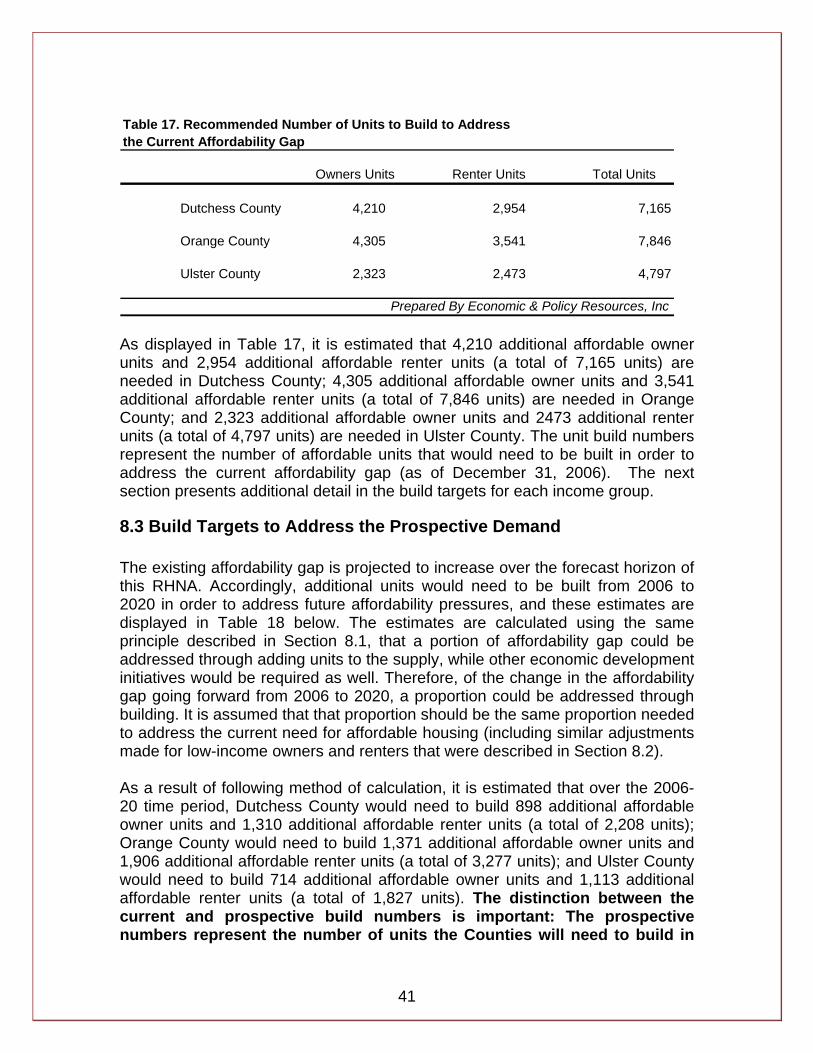
41

Table 17. Recommended Number of Units to Build to Addressthe Current Affordability Gap

Owners Units Renter Units Total Units

Dutchess County 4,210 2,954 7,165

Orange County 4,305 3,541 7,846

Ulster County 2,323 2,473 4,797

Prepared By Economic & Policy Resources, Inc As displayed in Table 17, it is estimated that 4,210 additional affordable owner units and 2,954 additional affordable renter units (a total of 7,165 units) are needed in Dutchess County; 4,305 additional affordable owner units and 3,541 additional affordable renter units (a total of 7,846 units) are needed in Orange County; and 2,323 additional affordable owner units and 2473 additional renter units (a total of 4,797 units) are needed in Ulster County. The unit build numbers represent the number of affordable units that would need to be built in order to address the current affordability gap (as of December 31, 2006). The next section presents additional detail in the build targets for each income group.

8.3 Build Targets to Address the Prospective Demand The existing affordability gap is projected to increase over the forecast horizon of this RHNA. Accordingly, additional units would need to be built from 2006 to 2020 in order to address future affordability pressures, and these estimates are displayed in Table 18 below. The estimates are calculated using the same principle described in Section 8.1, that a portion of affordability gap could be addressed through adding units to the supply, while other economic development initiatives would be required as well. Therefore, of the change in the affordability gap going forward from 2006 to 2020, a proportion could be addressed through building. It is assumed that that proportion should be the same proportion needed to address the current need for affordable housing (including similar adjustments made for low-income owners and renters that were described in Section 8.2). As a result of following method of calculation, it is estimated that over the 2006-20 time period, Dutchess County would need to build 898 additional affordable owner units and 1,310 additional affordable renter units (a total of 2,208 units); Orange County would need to build 1,371 additional affordable owner units and 1,906 additional affordable renter units (a total of 3,277 units); and Ulster County would need to build 714 additional affordable owner units and 1,113 additional affordable renter units (a total of 1,827 units). The distinction between the current and prospective build numbers is important: The prospective numbers represent the number of units the Counties will need to build in

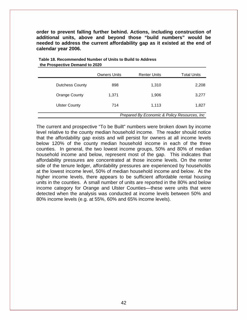
42

order to prevent falling further behind. Actions, including construction of additional units, above and beyond those “build numbers” would be needed to address the current affordability gap as it existed at the end of calendar year 2006.

Table 18. Recommended Number of Units to Build to Address the Prospective Demand to 2020

Owners Units Renter Units Total Units

Dutchess County 898 1,310 2,208

Orange County 1,371 1,906 3,277

Ulster County 714 1,113 1,827

Prepared By Economic & Policy Resources, Inc The current and prospective “To be Built” numbers were broken down by income level relative to the county median household income. The reader should notice that the affordability gap exists and will persist for owners at all income levels below 120% of the county median household income in each of the three counties. In general, the two lowest income groups, 50% and 80% of median household income and below, represent most of the gap. This indicates that affordability pressures are concentrated at those income levels. On the renter side of the tenure ledger, affordability pressures are experienced by households at the lowest income level, 50% of median household income and below. At the higher income levels, there appears to be sufficient affordable rental housing units in the counties. A small number of units are reported in the 80% and below income category for Orange and Ulster Counties—these were units that were detected when the analysis was conducted at income levels between 50% and 80% income levels (e.g. at 55%, 60% and 65% income levels).

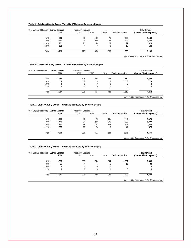
43

Table 19. Dutchess County Owner "To be Built" Numbers By Income Category

% of Median HH Income Current Demand Total Demand2006 2010 2015 2020 Total Prospective (Current Plus Prospective)

50% 962 30 100 76 205 1,16880% 2,182 75 280 234 588 2,770

100% 931 21 48 23 92 1,023120% 135 4 9 0 13 148

Total 4,210 129 436 333 898 5,108


Table 20. Dutchess County Renter "To be Built" Numbers By Income Category


50% 2,954 325 556 428 1,310 4,26480% 0 0 0 0 0 0

100% 0 0 0 0 0 0120% 0 0 0 0 0 0

Total 2,954 325 556 428 1,310 4,264


Prospective Demand

Prospective Demand

Table 21. Orange County Owner "To be Built" Numbers By Income Category


50% 1,195 66 170 145 381 1,57680% 1,443 94 283 276 653 2,097

100% 1,333 58 134 102 295 1,628120% 333 18 24 0 42 375

Total 4305 236 611 524 1371 5,676


Table 22. Orange County Renter "To be Built" Numbers By Income Category


50% 3,518 503 744 644 1,891 5,40980% 23 4 6 5 15 38

100% 0 0 0 0 0 0120% 0 0 0 0 0 0

Total 3,541 508 749 649 1,906 5,447


Prospective Demand

Prospective Demand

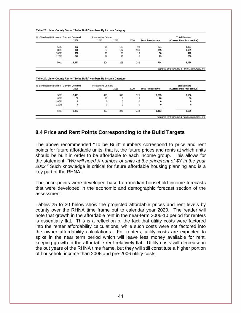
44

Table 23. Ulster County Owner "To be Built" Numbers By Income Category


50% 892 79 103 93 274 1,16780% 826 87 132 136 355 1,181

100% 366 23 20 13 56 422120% 240 16 13 0 29 268

Total 2,323 204 268 242 714 3,038


Table 24. Ulster County Renter "To be Built" Numbers By Income Category


50% 2,421 419 340 326 1,085 3,50680% 52 12 8 8 28 80

100% 0 0 0 0 0 0120% 0 0 0 0 0 0

Total 2,473 431 348 334 1,113 3,586


Prospective Demand

Prospective Demand

8.4 Price and Rent Points Corresponding to the Build Targets The above recommended “To be Built” numbers correspond to price and rent points for future affordable units, that is, the future prices and rents at which units should be built in order to be affordable to each income group. This allows for the statement: “We will need X number of units at the price/rent of $Y in the year 20xx.” Such knowledge is critical for future affordable housing planning and is a key part of the RHNA. The price points were developed based on median household income forecasts that were developed in the economic and demographic forecast section of the assessment. Tables 25 to 30 below show the projected affordable prices and rent levels by county over the RHNA time frame out to calendar year 2020. The reader will note that growth in the affordable rent in the near-term 2006-10 period for renters is essentially flat. This is a reflection of the fact that utility costs were factored into the renter affordability calculations, while such costs were not factored into the owner affordability calculations. For renters, utility costs are expected to spike in the near term period which will leave less money available for rent, keeping growth in the affordable rent relatively flat. Utility costs will decrease in the out years of the RHNA time frame, but they will still constitute a higher portion of household income than 2006 and pre-2006 utility costs.

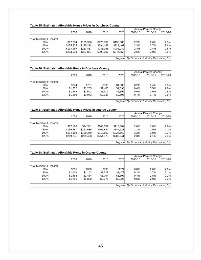
45

Table 25. Estimated Affordable House Prices in Dutchess County

2006 2010 2015 2020 2006-10 2010-15 2015-20

% of Median HH Income50% $97,084 $105,926 $120,139 $135,888 2.2% 2.6% 2.5%80% $155,335 $170,294 $194,482 $221,467 2.3% 2.7% 2.6%100% $194,169 $213,887 $245,956 $281,980 2.4% 2.8% 2.8%120% $233,003 $257,891 $298,607 $344,656 2.6% 3.0% 2.9%


Table 26. Estimated Affordable Rents in Dutchess County

2006 2010 2015 2020 2006-10 2010-15 2015-20

% of Median HH Income50% $744 $751 $886 $1,003 0.2% 3.4% 2.5%80% $1,232 $1,253 $1,486 $1,693 0.4% 3.5% 2.6%100% $1,565 $1,602 $1,912 $2,192 0.6% 3.6% 2.8%120% $1,889 $1,943 $2,335 $2,696 0.7% 3.7% 2.9%


Annual Percent Change


Table 27. Estimated Affordable House Prices in Orange County

2006 2010 2015 2020 2006-10 2010-15 2015-20



Table 28. Estimated Affordable Rents in Orange County

2006 2010 2015 2020 2006-10 2010-15 2015-20

% of Median HH Income50% $695 $696 $793 $874 0.0% 2.6% 2.0%80% $1,153 $1,163 $1,329 $1,473 0.2% 2.7% 2.1%100% $1,463 $1,484 $1,704 $1,898 0.4% 2.8% 2.2%120% $1,766 $1,800 $2,076 $2,326 0.5% 2.9% 2.3%




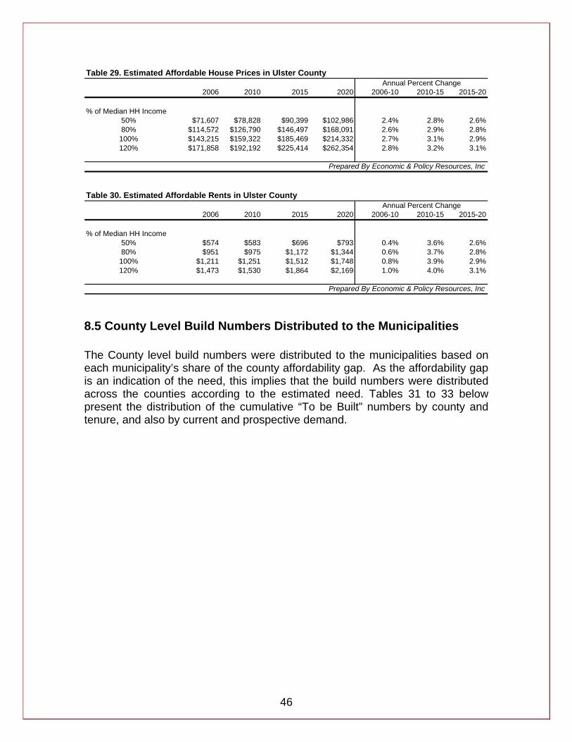
46

Table 29. Estimated Affordable House Prices in Ulster County

2006 2010 2015 2020 2006-10 2010-15 2015-20



Table 30. Estimated Affordable Rents in Ulster County

2006 2010 2015 2020 2006-10 2010-15 2015-20

% of Median HH Income50% $574 $583 $696 $793 0.4% 3.6% 2.6%80% $951 $975 $1,172 $1,344 0.6% 3.7% 2.8%100% $1,211 $1,251 $1,512 $1,748 0.8% 3.9% 2.9%120% $1,473 $1,530 $1,864 $2,169 1.0% 4.0% 3.1%




8.5 County Level Build Numbers Distributed to the Municipalities The County level build numbers were distributed to the municipalities based on each municipality’s share of the county affordability gap. As the affordability gap is an indication of the need, this implies that the build numbers were distributed across the counties according to the estimated need. Tables 31 to 33 below present the distribution of the cumulative “To be Built” numbers by county and tenure, and also by current and prospective demand.

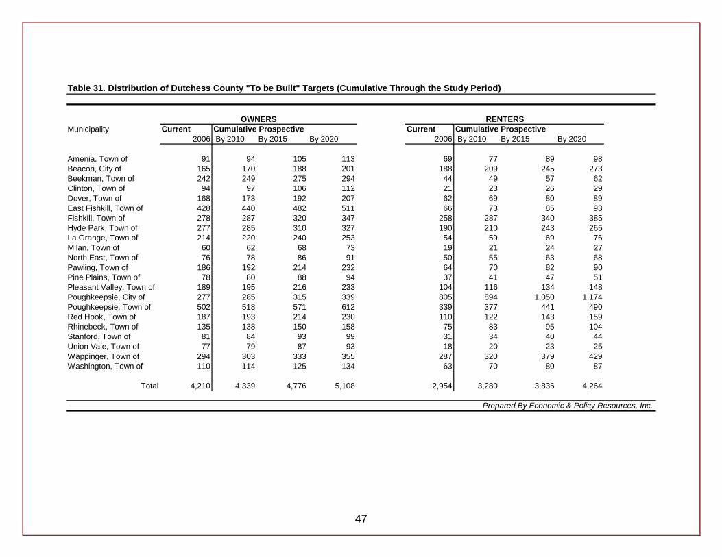
47

Table 31. Distribution of Dutchess County "To be Built" Targets (Cumulative Through the Study Period)

Municipality Current Cumulative Prospective Current Cumulative Prospective2006 By 2010 By 2015 By 2020 2006 By 2010 By 2015 By 2020

Amenia, Town of 91 94 105 113 69 77 89 98Beacon, City of 165 170 188 201 188 209 245 273Beekman, Town of 242 249 275 294 44 49 57 62Clinton, Town of 94 97 106 112 21 23 26 29Dover, Town of 168 173 192 207 62 69 80 89East Fishkill, Town of 428 440 482 511 66 73 85 93Fishkill, Town of 278 287 320 347 258 287 340 385Hyde Park, Town of 277 285 310 327 190 210 243 265La Grange, Town of 214 220 240 253 54 59 69 76Milan, Town of 60 62 68 73 19 21 24 27North East, Town of 76 78 86 91 50 55 63 68Pawling, Town of 186 192 214 232 64 70 82 90Pine Plains, Town of 78 80 88 94 37 41 47 51Pleasant Valley, Town of 189 195 216 233 104 116 134 148Poughkeepsie, City of 277 285 315 339 805 894 1,050 1,174Poughkeepsie, Town of 502 518 571 612 339 377 441 490Red Hook, Town of 187 193 214 230 110 122 143 159Rhinebeck, Town of 135 138 150 158 75 83 95 104Stanford, Town of 81 84 93 99 31 34 40 44Union Vale, Town of 77 79 87 93 18 20 23 25Wappinger, Town of 294 303 333 355 287 320 379 429Washington, Town of 110 114 125 134 63 70 80 87

Total 4,210 4,339 4,776 5,108 2,954 3,280 3,836 4,264

Prepared By Economic & Policy Resources, Inc.

RENTERSOWNERS

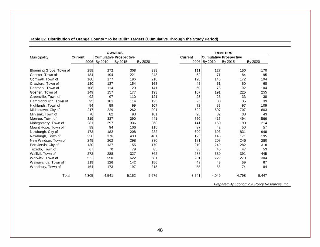
48

Table 32. Distribution of Orange County "To be Built" Targets (Cumulative Through the Study Period)


Blooming Grove, Town of 258 272 308 338 111 127 150 170Chester, Town of 184 194 221 243 62 71 84 95Cornwall, Town of 168 177 196 210 128 146 172 194Crawford, Town of 130 137 154 168 45 51 60 68Deerpark, Town of 108 114 129 141 69 78 92 104Goshen, Town of 149 157 177 193 167 191 225 255Greenville, Town of 92 97 110 121 25 28 33 38Hamptonburgh, Town of 95 101 114 125 26 30 35 39Highlands, Town of 84 89 99 107 72 83 97 109Middletown, City of 217 229 262 291 522 597 707 803Minisink, Town of 78 82 93 101 28 32 38 43Monroe, Town of 319 337 390 441 360 413 494 566Montgomery, Town of 281 297 336 368 141 160 190 214Mount Hope, Town of 89 94 106 115 37 42 50 57Newburgh, City of 173 182 208 232 609 698 831 948Newburgh, Town of 356 376 430 481 125 143 171 195New Windsor, Town of 249 262 298 330 181 208 246 280Port Jervis, City of 130 137 155 170 210 240 282 318Tuxedo, Town of 67 70 79 85 35 40 47 53Wallkill, Town of 272 288 327 362 288 330 391 445Warwick, Town of 522 550 622 681 201 229 270 304Wawayanda, Town of 119 126 142 156 43 49 59 67Woodbury, Town of 164 173 197 218 55 63 74 84

Total 4,305 4,541 5,152 5,676 3,541 4,049 4,798 5,447


RENTERSOWNERS

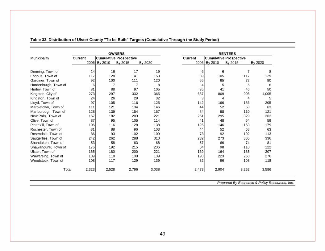
49

Table 33. Distribution of Ulster County "To be Built" Targets (Cumulative Through the Study Period)


Denning, Town of 14 16 17 19 6 6 7 8Esopus, Town of 117 128 141 153 89 105 117 129Gardiner, Town of 92 100 111 120 55 65 72 80Hardenburgh, Town of 6 7 7 8 4 5 5 6Hurley, Town of 81 88 97 105 35 41 46 50Kingston, City of 273 297 332 365 687 809 908 1,005Kingston, Town of 24 26 29 32 3 4 4 5Lloyd, Town of 97 105 116 125 142 166 186 205Marbletown, Town of 111 121 134 146 44 52 58 63Marlborough, Town of 128 139 154 167 84 98 110 121New Paltz, Town of 167 182 203 221 251 295 329 362Olive, Town of 87 95 105 114 41 48 54 59Plattekill, Town of 106 116 128 138 125 146 163 179Rochester, Town of 81 88 96 103 44 52 58 63Rosendale, Town of 86 93 102 109 78 92 102 113Saugerties, Town of 242 262 288 310 232 273 305 336Shandaken, Town of 53 58 63 68 57 66 74 81Shawangunk, Town of 176 192 215 236 84 98 110 122Ulster, Town of 165 180 200 221 139 164 185 207Wawarsing, Town of 109 118 130 139 190 223 250 276Woodstock, Town of 108 117 129 139 82 96 108 118

Total 2,323 2,528 2,796 3,038 2,473 2,904 3,252 3,586


RENTERSOWNERS

50

9. Conclusions The affordable housing challenge likely acts as a barrier to overall economic development and has emerged as an important issue in the 3-County region. This RHNA serves as a baseline assessment of housing needs in the 3-County region. The intent is to inform decision-makers in the region and to facilitate implementation of solutions. The RHNA provides municipal governments with the data necessary to position themselves well to meet the housing needs of their residents out to 2020, and successful implementation of solutions will likely be a necessity for future robust economic growth in the region. As of 2006, a substantial number of the region’s residents found themselves in increasingly untenable positions, and this situation has likely continued through 2007 and 2008, even after recent price declines in for-sale housing. The affordability situation in the region has been affected by several factors: (1) the housing market expansion of the late 1990s and mid-2000s exacerbated the affordability situation in the region as house prices grew rapidly and household income did not keep up; (2) An in-flow of new residents coming from surrounding metro areas (such as the New York metro area) that has resulted in increased demand for housing along the price spectrum which has placed significant upward pressures on housing prices throughout the 3-Ccounty area; (3) community resistance and perceptions about affordable housing has been cited as obstacle to affordable housing development; and (4) the regional economy has been challenged to retain good-paying jobs—particularly those in the manufacturing sector. Currently, the U.S. economy is in a recession. The national economy is contracting in terms of output and shedding payroll jobs, while the unemployment rate has increased substantially over the last year. Indicators also suggest that the housing market is going through what is in many ways the worst downturn since the 1930s, as construction and prices have decreased from peaks in 2007. The economy’s troubles are not likely to be resolved quickly, demonstrated by, and perhaps even exacerbated by, the government’s willingness to intervene in the market as of February of 2009. While the intervention has probably been necessary to avert even further problems in the economy, such a government presence in the market will likely result in a slow and protracted recovery. This has implications for housing the 3-County region: with housing price declines expected in the near term period, residents may see some temporary relief in terms of affordability. However, It is unlikely that the decline in house prices will alleviate affordability pressures to the same extent that rapid growth in house prices during the early 2000s contributed to those affordability pressures. At the national level, affordability indicators as of February 2009 indicate that pressures have subsided to some degree due to price declines. This relief, however, is likely to be short-lived. Once the national economy recovers from the current

51

downturn, affordability pressures are likely to reemerge and increasingly burden both owner and renter households. Although affordability challenges have gained prominence and are increasingly in the public spot light, most current data is limited at the county level, and for the most part, non-existent at the municipal level. This assessment is an effort to address this information gap and provide decision makers and local planning leaders with estimates of affordable housing needs in the 3-County region. The estimates were made for the “current” period (2006 was the base year of the study) and based on affordable prices that were determined by factoring in estimated costs associated with owning and renting, for income levels relative to median household income at the county level. The estimates of current need were followed by estimates of prospective housing needs for each county through calendar year 2020. The current and prospective housing unit needs were then complemented with price points for owners and rent levels for renter units. For owners and renters, estimates were also made of the portion of the needed units by tenure category that might be constructed as part of a comprehensive demand and supply approach to address the estimated affordability gap. These estimates were made for each of the three counties, and also for the 66 municipalities in the region.

52

Appendices The following section includes report appendices that provide additional detail on the methods and data used in the study. All of the estimates developed in the study were thoroughly reviewed by the project technical review committee before being approved for use in the report. The project technical review committee was briefed on and approved all steps taken in the study through a series of Technical Memos, which are the source documents for much of the material presented in the following appendices.

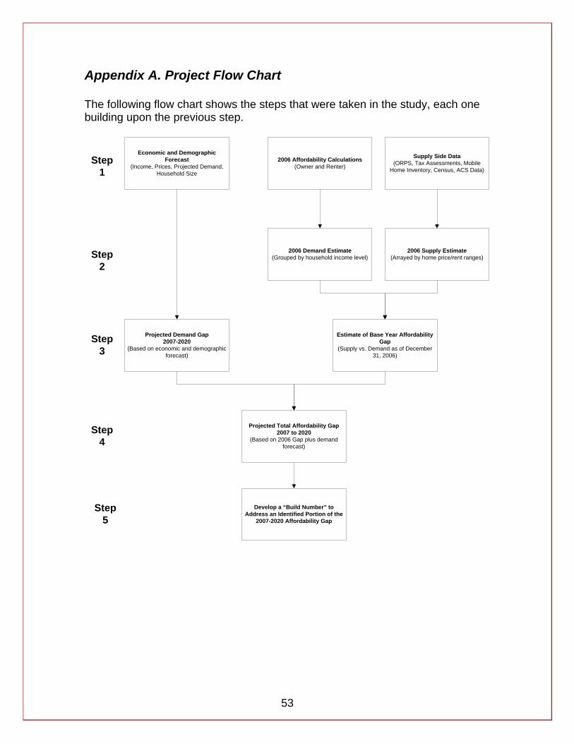
53

Appendix A. Project Flow Chart The following flow chart shows the steps that were taken in the study, each one building upon the previous step.

Economic and DemographicForecast

(Income, Prices, Projected Demand,Household Size

2006 Affordability Calculations(Owner and Renter)

Supply Side Data(ORPS, Tax Assessments, Mobile

Home Inventory, Census, ACS Data)

2006 Demand Estimate(Grouped by household income level)

2006 Supply Estimate(Arrayed by home price/rent ranges)

Estimate of Base Year AffordabilityGap

(Supply vs. Demand as of December31, 2006)

Projected Demand Gap2007-2020

(Based on economic and demographicforecast)

Projected Total Affordability Gap2007 to 2020

(Based on 2006 Gap plus demandforecast)

Develop a “Build Number” toAddress an Identified Portion of the

2007-2020 Affordability Gap

Step1

Step2

Step3

Step4

Step5

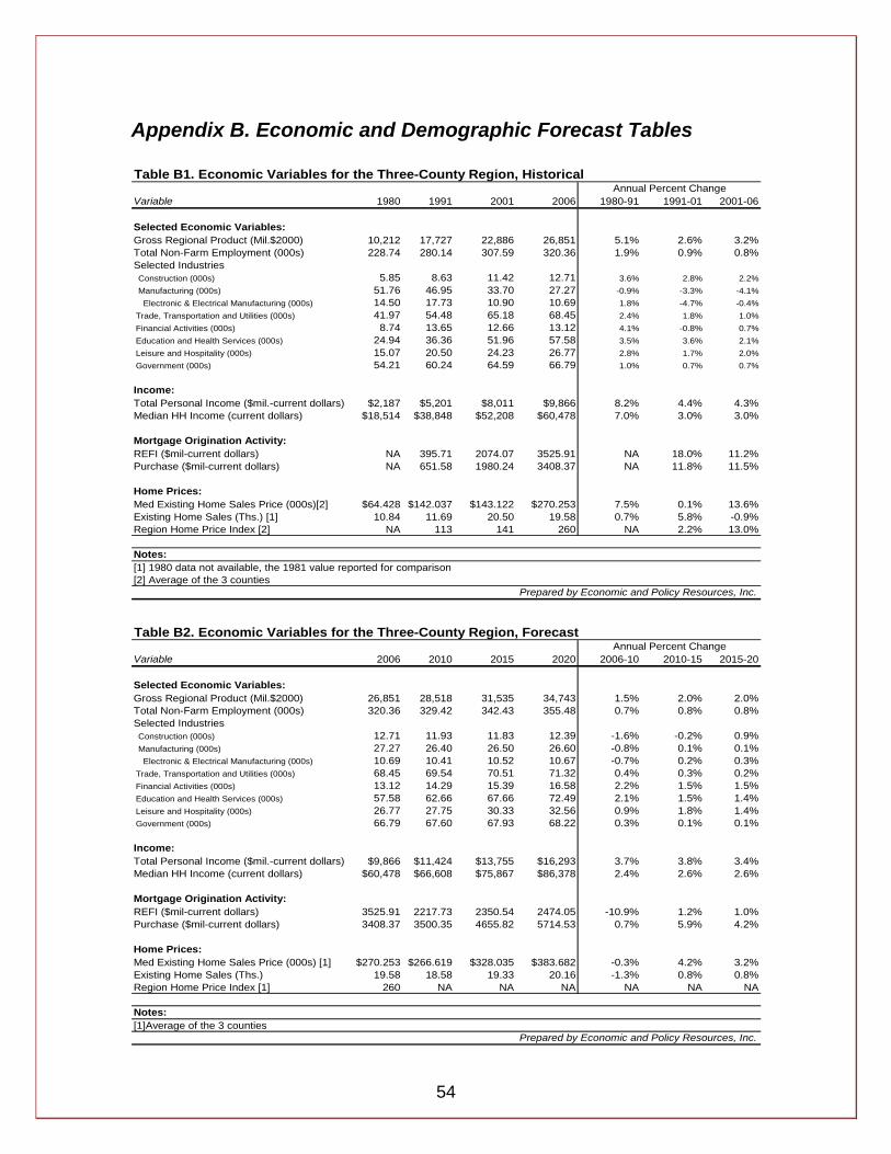
54

Appendix B. Economic and Demographic Forecast Tables Table B1. Economic Variables for the Three-County Region, Historical

Variable 1980 1991 2001 2006 1980-91 1991-01 2001-06

Selected Economic Variables:Gross Regional Product (Mil.$2000) 10,212 17,727 22,886 26,851 5.1% 2.6% 3.2%Total Non-Farm Employment (000s) 228.74 280.14 307.59 320.36 1.9% 0.9% 0.8%Selected Industries Construction (000s) 5.85 8.63 11.42 12.71 3.6% 2.8% 2.2% Manufacturing (000s) 51.76 46.95 33.70 27.27 -0.9% -3.3% -4.1% Electronic & Electrical Manufacturing (000s) 14.50 17.73 10.90 10.69 1.8% -4.7% -0.4% Trade, Transportation and Utilities (000s) 41.97 54.48 65.18 68.45 2.4% 1.8% 1.0% Financial Activities (000s) 8.74 13.65 12.66 13.12 4.1% -0.8% 0.7% Education and Health Services (000s) 24.94 36.36 51.96 57.58 3.5% 3.6% 2.1% Leisure and Hospitality (000s) 15.07 20.50 24.23 26.77 2.8% 1.7% 2.0% Government (000s) 54.21 60.24 64.59 66.79 1.0% 0.7% 0.7%

Income:Total Personal Income ($mil.-current dollars) $2,187 $5,201 $8,011 $9,866 8.2% 4.4% 4.3%Median HH Income (current dollars) $18,514 $38,848 $52,208 $60,478 7.0% 3.0% 3.0%

Mortgage Origination Activity:REFI ($mil-current dollars) NA 395.71 2074.07 3525.91 NA 18.0% 11.2%Purchase ($mil-current dollars) NA 651.58 1980.24 3408.37 NA 11.8% 11.5%

Home Prices:Med Existing Home Sales Price (000s)[2] $64.428 $142.037 $143.122 $270.253 7.5% 0.1% 13.6%Existing Home Sales (Ths.) [1] 10.84 11.69 20.50 19.58 0.7% 5.8% -0.9%Region Home Price Index [2] NA 113 141 260 NA 2.2% 13.0%

Notes:[1] 1980 data not available, the 1981 value reported for comparison[2] Average of the 3 counties

Table B2. Economic Variables for the Three-County Region, Forecast

Variable 2006 2010 2015 2020 2006-10 2010-15 2015-20

Selected Economic Variables:Gross Regional Product (Mil.$2000) 26,851 28,518 31,535 34,743 1.5% 2.0% 2.0%Total Non-Farm Employment (000s) 320.36 329.42 342.43 355.48 0.7% 0.8% 0.8%Selected Industries Construction (000s) 12.71 11.93 11.83 12.39 -1.6% -0.2% 0.9% Manufacturing (000s) 27.27 26.40 26.50 26.60 -0.8% 0.1% 0.1% Electronic & Electrical Manufacturing (000s) 10.69 10.41 10.52 10.67 -0.7% 0.2% 0.3% Trade, Transportation and Utilities (000s) 68.45 69.54 70.51 71.32 0.4% 0.3% 0.2% Financial Activities (000s) 13.12 14.29 15.39 16.58 2.2% 1.5% 1.5% Education and Health Services (000s) 57.58 62.66 67.66 72.49 2.1% 1.5% 1.4% Leisure and Hospitality (000s) 26.77 27.75 30.33 32.56 0.9% 1.8% 1.4% Government (000s) 66.79 67.60 67.93 68.22 0.3% 0.1% 0.1%


Mortgage Origination Activity:REFI ($mil-current dollars) 3525.91 2217.73 2350.54 2474.05 -10.9% 1.2% 1.0%Purchase ($mil-current dollars) 3408.37 3500.35 4655.82 5714.53 0.7% 5.9% 4.2%

Home Prices:Med Existing Home Sales Price (000s) [1] $270.253 $266.619 $328.035 $383.682 -0.3% 4.2% 3.2%Existing Home Sales (Ths.) 19.58 18.58 19.33 20.16 -1.3% 0.8% 0.8%Region Home Price Index [1] 260 NA NA NA NA NA NA

Notes:[1]Average of the 3 counties





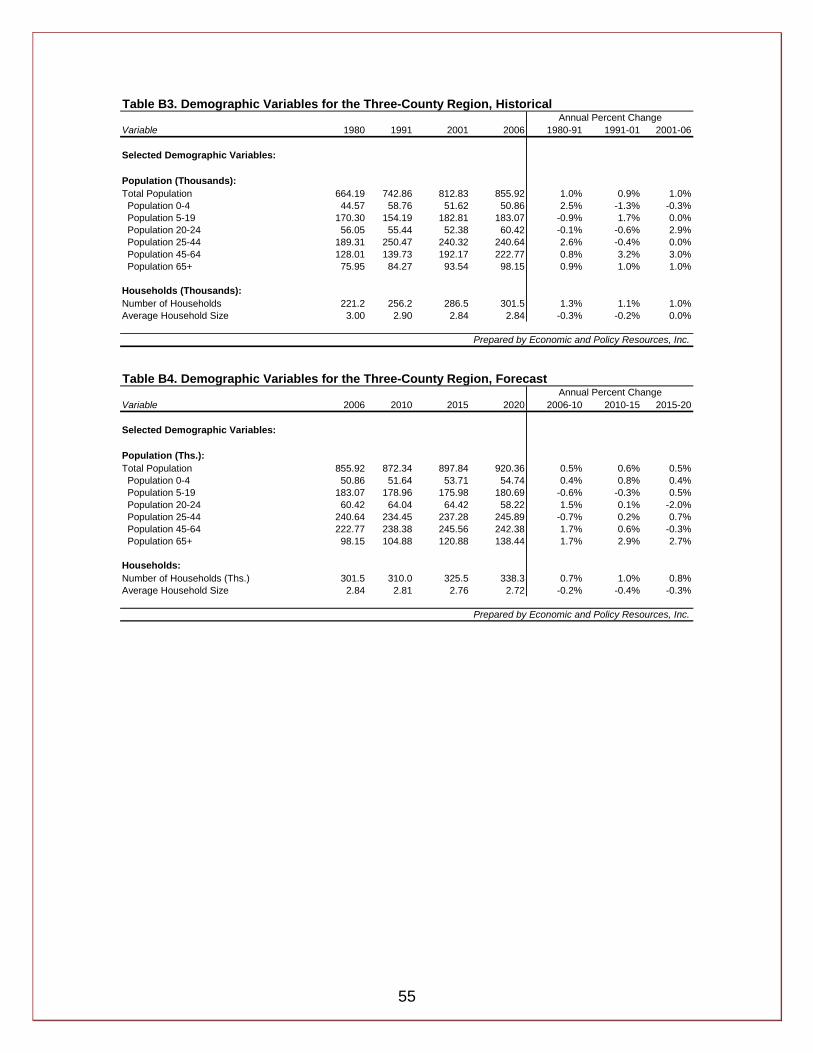
55

Table B3. Demographic Variables for the Three-County Region, Historical

Variable 1980 1991 2001 2006 1980-91 1991-01 2001-06

Selected Demographic Variables:

Population (Thousands):Total Population 664.19 742.86 812.83 855.92 1.0% 0.9% 1.0% Population 0-4 44.57 58.76 51.62 50.86 2.5% -1.3% -0.3% Population 5-19 170.30 154.19 182.81 183.07 -0.9% 1.7% 0.0% Population 20-24 56.05 55.44 52.38 60.42 -0.1% -0.6% 2.9% Population 25-44 189.31 250.47 240.32 240.64 2.6% -0.4% 0.0% Population 45-64 128.01 139.73 192.17 222.77 0.8% 3.2% 3.0% Population 65+ 75.95 84.27 93.54 98.15 0.9% 1.0% 1.0%

Households (Thousands):Number of Households 221.2 256.2 286.5 301.5 1.3% 1.1% 1.0%Average Household Size 3.00 2.90 2.84 2.84 -0.3% -0.2% 0.0%

Table B4. Demographic Variables for the Three-County Region, Forecast

Variable 2006 2010 2015 2020 2006-10 2010-15 2015-20


Population (Ths.):Total Population 855.92 872.34 897.84 920.36 0.5% 0.6% 0.5% Population 0-4 50.86 51.64 53.71 54.74 0.4% 0.8% 0.4% Population 5-19 183.07 178.96 175.98 180.69 -0.6% -0.3% 0.5% Population 20-24 60.42 64.04 64.42 58.22 1.5% 0.1% -2.0% Population 25-44 240.64 234.45 237.28 245.89 -0.7% 0.2% 0.7% Population 45-64 222.77 238.38 245.56 242.38 1.7% 0.6% -0.3% Population 65+ 98.15 104.88 120.88 138.44 1.7% 2.9% 2.7%

Households:Number of Households (Ths.) 301.5 310.0 325.5 338.3 0.7% 1.0% 0.8%Average Household Size 2.84 2.81 2.76 2.72 -0.2% -0.4% -0.3%





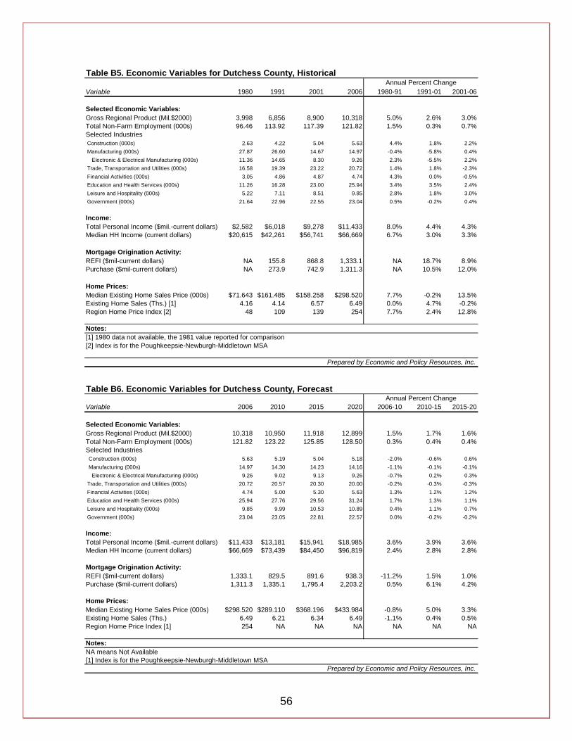
56

Table B5. Economic Variables for Dutchess County, Historical

Variable 1980 1991 2001 2006 1980-91 1991-01 2001-06

Selected Economic Variables:Gross Regional Product (Mil.$2000) 3,998 6,856 8,900 10,318 5.0% 2.6% 3.0%Total Non-Farm Employment (000s) 96.46 113.92 117.39 121.82 1.5% 0.3% 0.7%Selected Industries Construction (000s) 2.63 4.22 5.04 5.63 4.4% 1.8% 2.2% Manufacturing (000s) 27.87 26.60 14.67 14.97 -0.4% -5.8% 0.4% Electronic & Electrical Manufacturing (000s) 11.36 14.65 8.30 9.26 2.3% -5.5% 2.2% Trade, Transportation and Utilities (000s) 16.58 19.39 23.22 20.72 1.4% 1.8% -2.3% Financial Activities (000s) 3.05 4.86 4.87 4.74 4.3% 0.0% -0.5% Education and Health Services (000s) 11.26 16.28 23.00 25.94 3.4% 3.5% 2.4% Leisure and Hospitality (000s) 5.22 7.11 8.51 9.85 2.8% 1.8% 3.0% Government (000s) 21.64 22.96 22.55 23.04 0.5% -0.2% 0.4%


Mortgage Origination Activity:REFI ($mil-current dollars) NA 155.8 868.8 1,333.1 NA 18.7% 8.9%Purchase ($mil-current dollars) NA 273.9 742.9 1,311.3 NA 10.5% 12.0%

Home Prices:Median Existing Home Sales Price (000s) $71.643 $161.485 $158.258 $298.520 7.7% -0.2% 13.5%Existing Home Sales (Ths.) [1] 4.16 4.14 6.57 6.49 0.0% 4.7% -0.2%Region Home Price Index [2] 48 109 139 254 7.7% 2.4% 12.8%

Notes:[1] 1980 data not available, the 1981 value reported for comparison[2] Index is for the Poughkeepsie-Newburgh-Middletown MSA

Table B6. Economic Variables for Dutchess County, Forecast

Variable 2006 2010 2015 2020 2006-10 2010-15 2015-20

Selected Economic Variables:Gross Regional Product (Mil.$2000) 10,318 10,950 11,918 12,899 1.5% 1.7% 1.6%Total Non-Farm Employment (000s) 121.82 123.22 125.85 128.50 0.3% 0.4% 0.4%Selected Industries Construction (000s) 5.63 5.19 5.04 5.18 -2.0% -0.6% 0.6% Manufacturing (000s) 14.97 14.30 14.23 14.16 -1.1% -0.1% -0.1% Electronic & Electrical Manufacturing (000s) 9.26 9.02 9.13 9.26 -0.7% 0.2% 0.3% Trade, Transportation and Utilities (000s) 20.72 20.57 20.30 20.00 -0.2% -0.3% -0.3% Financial Activities (000s) 4.74 5.00 5.30 5.63 1.3% 1.2% 1.2% Education and Health Services (000s) 25.94 27.76 29.56 31.24 1.7% 1.3% 1.1% Leisure and Hospitality (000s) 9.85 9.99 10.53 10.89 0.4% 1.1% 0.7% Government (000s) 23.04 23.05 22.81 22.57 0.0% -0.2% -0.2%


Mortgage Origination Activity:REFI ($mil-current dollars) 1,333.1 829.5 891.6 938.3 -11.2% 1.5% 1.0%Purchase ($mil-current dollars) 1,311.3 1,335.1 1,795.4 2,203.2 0.5% 6.1% 4.2%

Home Prices:Median Existing Home Sales Price (000s) $298.520 $289.110 $368.196 $433.984 -0.8% 5.0% 3.3%Existing Home Sales (Ths.) 6.49 6.21 6.34 6.49 -1.1% 0.4% 0.5%Region Home Price Index [1] 254 NA NA NA NA NA NA

Notes:NA means Not Available[1] Index is for the Poughkeepsie-Newburgh-Middletown MSA





57

Table B7. Demographic Variables for Dutchess County, Historical

Variable 1980 1991 2001 2006 1980-91 1991-01 2001-06


Population (Thousands):Total Population 245.40 261.95 284.86 295.14 0.6% 0.8% 0.7% Population 0-4 15.40 19.40 16.94 16.19 2.1% -1.3% -0.9% Population 5-19 62.38 52.42 62.18 61.35 -1.6% 1.7% -0.3% Population 20-24 21.05 20.09 18.71 21.48 -0.4% -0.7% 2.8% Population 25-44 71.18 88.96 84.97 81.96 2.0% -0.5% -0.7% Population 45-64 48.17 51.00 67.83 77.73 0.5% 2.9% 2.8% Population 65+ 27.22 30.07 34.23 36.43 0.9% 1.3% 1.3%


Table B8. Demographic Variables for Dutchess County, Forecast

Variable 2006 2010 2015 2020 2006-10 2010-15 2015-20


Population (Ths.):Total Population 295.14 297.57 305.63 311.83 0.2% 0.5% 0.4% Population 0-4 16.19 16.14 16.58 16.67 -0.1% 0.5% 0.1% Population 5-19 61.35 59.31 58.20 59.49 -0.8% -0.4% 0.4% Population 20-24 21.48 22.65 23.04 20.93 1.3% 0.3% -1.9% Population 25-44 81.96 77.98 76.95 77.60 -1.2% -0.3% 0.2% Population 45-64 77.73 82.18 84.34 82.63 1.4% 0.5% -0.4% Population 65+ 36.43 39.31 46.52 54.51 1.9% 3.4% 3.2%






58

Table B9. Economic Variables for Orange County, Historical

Variable 1980 1991 2001 2006 1980-91 1991-01 2001-06

Selected Economic Variables:Gross Regional Product (Mil.$2000) 3,989 7,087 9,521 11,417 5.4% 3.0% 3.7%Total Non-Farm Employment (000s) 82.49 106.13 125.76 133.73 2.3% 1.7% 1.2%Selected Industries Construction (000s) 2.13 3.27 4.68 4.96 4.0% 3.7% 1.2% Manufacturing (000s) 17.92 14.52 12.85 7.92 -1.9% -1.2% -9.2% Electronic & Electrical Manufacturing (000s) 1.63 1.65 1.89 0.79 0.1% 1.4% -15.9% Trade, Transportation and Utilities (000s) 16.07 23.65 29.39 35.34 3.6% 2.2% 3.8% Financial Activities (000s) 3.28 5.73 5.30 5.47 5.2% -0.8% 0.6% Education and Health Services (000s) 8.59 12.87 18.74 21.38 3.8% 3.8% 2.7% Leisure and Hospitality (000s) 5.13 7.82 9.12 9.93 3.9% 1.6% 1.7% Government (000s) 20.95 24.54 26.95 28.49 1.5% 0.9% 1.1%



Home Prices:Median Existing Home Sales Price (000s) $61.930 $144.657 $140.611 $260.464 8.0% -0.3% 13.1%Existing Home Sales (Ths.) [1] 4.18 4.50 9.53 8.34 0.7% 7.8% -2.6%Region Home Price Index [2] 48 109 139 254 7.7% 2.4% 12.8%

Notes:[1] 1980 data not available, the 1981 value reported for comparison[2] Index is for the Poughkeepsie-Newburgh-Middletown MSA

Table B10. Economic Variables for Orange County, Forecast

Variable 2006 2010 2015 2020 2006-10 2010-15 2015-20

Selected Economic Variables:Gross Regional Product (Mil.$2000) 11,417 12,194 13,725 15,417 1.7% 2.4% 2.4%Total Non-Farm Employment (000s) 133.73 138.80 146.23 153.91 0.9% 1.0% 1.0%Selected Industries Construction (000s) 4.96 4.61 4.63 4.92 -1.8% 0.1% 1.2% Manufacturing (000s) 7.92 7.77 8.00 8.23 -0.5% 0.6% 0.6% Electronic & Electrical Manufacturing (000s) 0.79 0.75 0.77 0.78 -1.3% 0.4% 0.4% Trade, Transportation and Utilities (000s) 35.34 36.13 37.12 38.07 0.6% 0.5% 0.5% Financial Activities (000s) 5.47 5.93 6.50 7.14 2.0% 1.9% 1.9% Education and Health Services (000s) 21.38 23.51 25.89 28.29 2.4% 2.0% 1.8% Leisure and Hospitality (000s) 9.93 10.35 11.29 12.07 1.0% 1.8% 1.4% Government (000s) 28.49 29.28 29.97 30.66 0.7% 0.5% 0.5%


Mortgage Origination Activity:REFI ($mil-current dollars) 1610.47 1002.12 1077.14 1133.51 -11.2% 1.5% 1.0%Purchase ($mil-current dollars) 1654.04 1684.12 2264.71 2779.14 0.5% 6.1% 4.2%

Home Prices:Median Existing Home Sales Price (000s) $260.464 $251.194 $314.511 $364.457 -0.9% 4.6% 3.0%Existing Home Sales (Ths.) 8.34 8.19 8.65 9.14 -0.4% 1.1% 1.1%Region Home Price Index [1] 254 NA NA NA NA NA NA

Notes:NA means Not Available[1] Index is for the Poughkeepsie-Newburgh-Middletown MSA





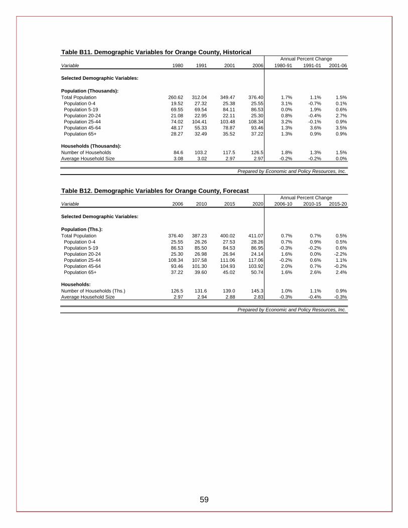
59

Table B11. Demographic Variables for Orange County, Historical

Variable 1980 1991 2001 2006 1980-91 1991-01 2001-06


Population (Thousands):Total Population 260.62 312.04 349.47 376.40 1.7% 1.1% 1.5% Population 0-4 19.52 27.32 25.38 25.55 3.1% -0.7% 0.1% Population 5-19 69.55 69.54 84.11 86.53 0.0% 1.9% 0.6% Population 20-24 21.08 22.95 22.11 25.30 0.8% -0.4% 2.7% Population 25-44 74.02 104.41 103.48 108.34 3.2% -0.1% 0.9% Population 45-64 48.17 55.33 78.87 93.46 1.3% 3.6% 3.5% Population 65+ 28.27 32.49 35.52 37.22 1.3% 0.9% 0.9%


Table B12. Demographic Variables for Orange County, Forecast

Variable 2006 2010 2015 2020 2006-10 2010-15 2015-20








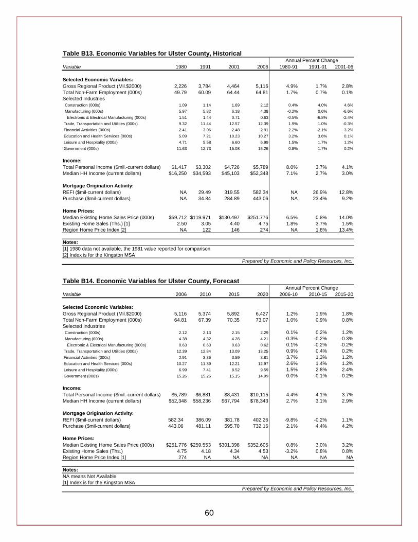
60

Table B13. Economic Variables for Ulster County, Historical

Variable 1980 1991 2001 2006 1980-91 1991-01 2001-06

Selected Economic Variables:Gross Regional Product (Mil.$2000) 2,226 3,784 4,464 5,116 4.9% 1.7% 2.8%Total Non-Farm Employment (000s) 49.79 60.09 64.44 64.81 1.7% 0.7% 0.1%Selected Industries Construction (000s) 1.09 1.14 1.69 2.12 0.4% 4.0% 4.6% Manufacturing (000s) 5.97 5.82 6.18 4.38 -0.2% 0.6% -6.6% Electronic & Electrical Manufacturing (000s) 1.51 1.44 0.71 0.63 -0.5% -6.8% -2.4% Trade, Transportation and Utilities (000s) 9.32 11.44 12.57 12.39 1.9% 1.0% -0.3% Financial Activities (000s) 2.41 3.06 2.48 2.91 2.2% -2.1% 3.2% Education and Health Services (000s) 5.09 7.21 10.23 10.27 3.2% 3.6% 0.1% Leisure and Hospitality (000s) 4.71 5.58 6.60 6.99 1.5% 1.7% 1.2% Government (000s) 11.63 12.73 15.08 15.26 0.8% 1.7% 0.2%



Home Prices:Median Existing Home Sales Price (000s) $59.712 $119.971 $130.497 $251.776 6.5% 0.8% 14.0%Existing Home Sales (Ths.) [1] 2.50 3.05 4.40 4.75 1.8% 3.7% 1.5%Region Home Price Index [2] NA 122 146 274 NA 1.8% 13.4%

Notes:[1] 1980 data not available, the 1981 value reported for comparison[2] Index is for the Kingston MSA

Table B14. Economic Variables for Ulster County, Forecast

Variable 2006 2010 2015 2020 2006-10 2010-15 2015-20

Selected Economic Variables:Gross Regional Product (Mil.$2000) 5,116 5,374 5,892 6,427 1.2% 1.9% 1.8%Total Non-Farm Employment (000s) 64.81 67.39 70.35 73.07 1.0% 0.9% 0.8%Selected Industries Construction (000s) 2.12 2.13 2.15 2.29 0.1% 0.2% 1.2% Manufacturing (000s) 4.38 4.32 4.28 4.21 -0.3% -0.2% -0.3% Electronic & Electrical Manufacturing (000s) 0.63 0.63 0.63 0.62 0.1% -0.2% -0.2% Trade, Transportation and Utilities (000s) 12.39 12.84 13.09 13.25 0.9% 0.4% 0.2% Financial Activities (000s) 2.91 3.36 3.59 3.81 3.7% 1.3% 1.2% Education and Health Services (000s) 10.27 11.39 12.21 12.97 2.6% 1.4% 1.2% Leisure and Hospitality (000s) 6.99 7.41 8.52 9.59 1.5% 2.8% 2.4% Government (000s) 15.26 15.26 15.15 14.99 0.0% -0.1% -0.2%


Mortgage Origination Activity:REFI ($mil-current dollars) 582.34 386.09 381.78 402.26 -9.8% -0.2% 1.1%Purchase ($mil-current dollars) 443.06 481.11 595.70 732.16 2.1% 4.4% 4.2%

Home Prices:Median Existing Home Sales Price (000s) $251.776 $259.553 $301.398 $352.605 0.8% 3.0% 3.2%Existing Home Sales (Ths.) 4.75 4.18 4.34 4.53 -3.2% 0.8% 0.8%Region Home Price Index [1] 274 NA NA NA NA NA NA

Notes:NA means Not Available[1] Index is for the Kingston MSA





61

Table B15. Demographic Variables for Ulster County, Historical

Variable 1980 1991 2001 2006 1980-91 1991-01 2001-06


Population (Thousands):Total Population 158.17 168.87 178.50 184.39 0.6% 0.6% 0.7% Population 0-4 9.64 12.04 9.30 9.12 2.0% -2.6% -0.4% Population 5-19 38.37 32.22 36.53 35.19 -1.6% 1.3% -0.7% Population 20-24 13.92 12.40 11.55 13.64 -1.0% -0.7% 3.4% Population 25-44 44.12 57.10 51.86 50.35 2.4% -1.0% -0.6% Population 45-64 31.66 33.39 45.47 51.58 0.5% 3.1% 2.6% Population 65+ 20.46 21.71 23.79 24.50 0.5% 0.9% 0.6%


Table B16. Demographic Variables for Ulster County, Forecast

Variable 2006 2010 2015 2020 2006-10 2010-15 2015-20








62

Appendix C. Housing Unit Demand Projections This appendix describes the approach and methods employed in developing the regional and county projections of housing unit demand. The projections utilized municipal and county level census data from 1990 to 2006 and were developed using an econometric model of household formation rates by age. Estimates of demand were developed for owner and renter units using the household projections presented in the economic and demographic forecast. Demand by age group was estimated using historical trends in each age group’s share of the county total as defined by the underlying economic and demographic forecast. The age groups were defined as 15 to 24 years, 25 to 44 years, 45 to 64 years, and 65 years and over. The trends in each age group were projected forward to 2020 to arrive at the results by tenure category and age group. The projections resulted in a slightly lower rate of housing unit demand growth than was the case during the 1990 to 2006 period. The projections also included a shift from owner to renter units during the period due to fundamental changes that are occurring in the current housing market which will affect housing demand over the forecast period. It is expected that home ownership rates will flatten—and decline in some age categories—in comparison to the past six to seven years in conjunction to the tighter, more expensive credit market conditions for mortgage financing. The housing unit demand projections indicate that the largest increase in housing unit demand in the 3-County region will be in the two older age groups, 45 to 64 years and 65 years and over, which are expected to exhibit strong rates of growth. Demand for units in the two younger age groups, aged 15 to 24 years and aged 25 to 44 years, will experience housing unit demand declines over the forecast period primarily due to the aging population. Overall, demand in the 3 County region is expected grow by 41,365 units by 2020 (or at an average annual rate of 2,954 units). Demand for owner units is expected to increase by 24,585 units by 2020 (or at an average annual rate of 1,756 units per year). Renter unit demand is expected to increase by 16,780 units (corresponding to an average annual increase of 1,198 units). These estimates correspond to an overall annual housing unit growth rate of 0.91%--consisting of a 0.78% annual rate for owner units, and a 1.18% annual rate of growth for renter unit demand over the forecast period. Tables H1 to H8 below show the demand projections for the 3-County region overall and for each county by tenure category and by age group.

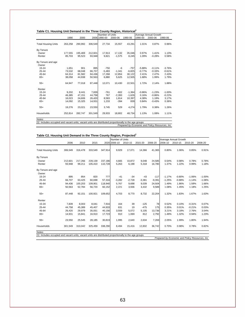
63

Table C1. Housing Unit Demand in the Three County Region, Historical1Number of Units Average Annual Growth

1990 2000 2006 1990-00 2000-06 1990-06 1990-00 2000-06 1990-06

Total Housing Units 263,258 290,992 306,549 27,734 15,557 43,291 1.01% 0.87% 0.96%

By Tenure Owner 177,555 195,469 212,601 17,913 17,132 35,046 0.97% 1.41% 1.13% Renter 85,703 95,523 93,948 9,821 -1,575 8,245 1.09% -0.28% 0.58%

By Tenure and age Owner 15-24 1,651 901 895 -750 -6 -757 -5.88% -0.11% -3.76% 25-44 73,532 68,048 66,707 -5,483 -1,341 -6,825 -0.77% -0.33% -0.61% 45-64 64,314 81,582 94,436 17,268 12,854 30,122 2.41% 2.47% 2.43% 65+ 38,058 44,938 50,563 6,880 5,625 12,505 1.68% 1.99% 1.79%

55+ 64,947 77,018 87,448 12,071 10,430 22,501 1.72% 2.14% 1.88%

Renter 15-24 9,202 8,441 7,839 -761 -602 -1,364 -0.86% -1.23% -1.00% 25-44 46,385 47,151 44,758 767 -2,393 -1,626 0.16% -0.86% -0.22% 45-64 16,023 24,606 26,420 8,583 1,814 10,397 4.38% 1.19% 3.17% 65+ 14,092 15,325 14,931 1,233 -394 839 0.84% -0.43% 0.36%

55+ 19,276 23,021 23,550 3,745 529 4,274 1.79% 0.38% 1.26%

Households 252,814 282,747 301,549 29,933 18,802 48,734 1.13% 1.08% 1.11%

Notes:[1] Includes occupied and vacant units; vacant units are distributed proportionally to the age groups


Table C2. Housing Unit Demand in the Three County Region, Projected1

Number of Units Average Annual Growth2006 2010 2015 2020 2006-10 2010-15 2015-20 2006-20 2006-10 2010-15 2015-20 2006-20

Total Housing Units 306,549 316,478 333,549 347,914 9,929 17,071 14,366 41,365 0.80% 1.06% 0.85% 0.91%

By Tenure Owner 212,601 217,266 228,139 237,186 4,665 10,872 9,048 24,585 0.54% 0.98% 0.78% 0.78% Renter 93,948 99,211 105,410 110,728 5,263 6,198 5,318 16,780 1.37% 1.22% 0.99% 1.18%

By Tenure and age Owner 15-24 895 854 820 777 -41 -34 -43 -117 -1.17% -0.80% -1.06% -1.00% 25-44 66,707 63,425 60,698 57,316 -3,282 -2,728 -3,381 -9,391 -1.25% -0.88% -1.14% -1.08% 45-64 94,436 100,203 109,901 118,940 5,767 9,698 9,039 24,504 1.49% 1.86% 1.59% 1.66% 65+ 50,563 52,784 56,720 60,152 2,221 3,936 3,432 9,589 1.08% 1.45% 1.18% 1.25%

55+ 87,448 92,151 100,921 109,652 4,703 8,770 8,732 22,204 1.32% 1.83% 1.67% 1.63%

Renter 15-24 7,839 8,003 8,041 7,916 164 39 -125 78 0.52% 0.10% -0.31% 0.07% 25-44 44,758 45,389 45,407 44,933 631 19 -475 175 0.35% 0.01% -0.21% 0.03% 45-64 26,420 29,979 35,051 40,156 3,559 5,072 5,105 13,736 3.21% 3.18% 2.76% 3.04% 65+ 14,931 15,841 16,910 17,723 910 1,069 812 2,792 1.49% 1.32% 0.94% 1.23%

55+ 23,550 25,545 28,185 30,819 1,995 2,640 2,634 7,269 2.05% 1.99% 1.80% 1.94%

Households 301,549 310,042 325,459 338,290 8,494 15,416 12,832 36,742 0.70% 0.98% 0.78% 0.82%



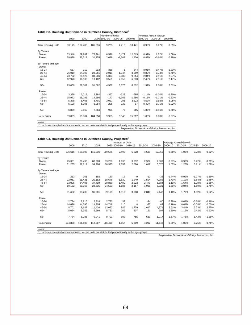
64

Table C3. Housing Unit Demand in Dutchess County, Historical1Number of Units Average Annual Growth

1990 2000 2006 1990-00 2000-06 1990-06 1990-00 2000-06 1990-06



By Tenure and age Owner 15-24 557 219 213 -338 -6 -344 -8.91% -0.47% -5.83% 25-44 26,019 24,008 22,961 -2,011 -1,047 -3,059 -0.80% -0.74% -0.78% 45-64 23,792 29,126 33,006 5,334 3,880 9,214 2.04% 2.11% 2.07% 65+ 12,978 16,530 19,182 3,551 2,652 6,203 2.45% 2.51% 2.47%

55+ 23,050 28,007 31,682 4,957 3,675 8,632 1.97% 2.08% 2.01%

Renter 15-24 3,379 3,012 2,784 -367 -228 -595 -1.14% -1.30% -1.20% 25-44 15,972 15,795 14,686 -177 -1,108 -1,286 -0.11% -1.21% -0.52% 45-64 5,378 8,405 8,701 3,027 296 3,323 4.57% 0.58% 3.05% 65+ 5,100 5,306 5,084 205 -222 -17 0.40% -0.71% -0.02%

55+ 6,869 7,860 7,784 991 -76 915 1.36% -0.16% 0.78%

Households 89,839 99,804 104,850 9,965 5,046 15,012 1.06% 0.83% 0.97%



Table C4. Housing Unit Demand in Dutchess County, Projected1




By Tenure and age Owner 15-24 213 201 192 180 -12 -9 -12 -33 -1.44% -0.92% -1.27% -1.19% 25-44 22,961 21,431 20,182 18,678 -1,530 -1,249 -1,504 -4,282 -1.71% -1.19% -1.54% -1.46% 45-64 33,006 34,496 37,419 39,889 1,490 2,923 2,470 6,884 1.11% 1.64% 1.29% 1.36% 65+ 19,182 20,368 22,535 24,503 1,186 2,167 1,968 5,321 1.51% 2.04% 1.69% 1.76%

55+ 31,682 33,200 36,281 39,129 1,519 3,080 2,848 7,447 1.18% 1.79% 1.52% 1.52%

Renter 15-24 2,784 2,816 2,818 2,723 32 2 -94 -60 0.29% 0.01% -0.68% -0.16% 25-44 14,686 14,796 14,805 14,748 110 8 -57 62 0.19% 0.01% -0.08% 0.03% 45-64 8,701 9,647 11,426 13,072 946 1,779 1,647 4,371 2.61% 3.44% 2.73% 2.95% 65+ 5,084 5,353 5,660 5,781 269 307 121 697 1.30% 1.12% 0.42% 0.92%

55+ 7,784 8,286 9,041 9,701 502 755 660 1,917 1.57% 1.76% 1.42% 1.58%

Households 104,850 106,508 112,207 116,499 1,657 5,699 4,292 11,648 0.39% 1.05% 0.75% 0.76%



65

Table C5. Housing Unit Demand in Orange County, Historical1Number of Units Average Annual Growth

1990 2000 2006 1990-00 2000-06 1990-06 1990-00 2000-06 1990-06



By Tenure and age Owner 15-24 639 468 486 -171 18 -153 -3.07% 0.64% -1.70% 25-44 31,042 29,607 30,383 -1,435 776 -659 -0.47% 0.43% -0.13% 45-64 24,914 32,433 39,626 7,519 7,193 14,712 2.67% 3.39% 2.94% 65+ 14,364 16,157 18,565 1,793 2,408 4,201 1.18% 2.34% 1.62%

55+ 24,223 28,625 34,198 4,402 5,573 9,975 1.68% 3.01% 2.18%

Renter 15-24 3,427 3,088 2,726 -339 -362 -701 -1.04% -2.06% -1.42% 25-44 19,456 19,763 18,813 307 -950 -643 0.16% -0.82% -0.21% 45-64 6,971 10,422 10,848 3,450 426 3,877 4.10% 0.67% 2.80% 65+ 5,627 6,410 6,169 783 -241 542 1.31% -0.64% 0.58%

55+ 7,898 9,855 10,074 1,957 219 2,176 2.24% 0.37% 1.53%

Households 101,892 115,376 126,549 13,484 11,173 24,657 1.25% 1.55% 1.36%


Prepared by Economic and Policy Resources, Inc ources, Inc

Table C6. Housing Unit Demand in Orange County, Projected1




By Tenure and age Owner 15-24 486 466 452 433 -20 -14 -19 -53 -1.05% -0.60% -0.86% -0.82% 25-44 30,383 29,130 28,277 27,096 -1,254 -853 -1,182 -3,288 -1.05% -0.59% -0.85% -0.81% 45-64 39,626 42,319 47,011 51,550 2,693 4,692 4,539 11,924 1.66% 2.13% 1.86% 1.90% 65+ 18,565 19,032 20,088 20,929 467 1,056 841 2,364 0.62% 1.09% 0.82% 0.86%

55+ 34,198 36,196 39,886 43,533 1,998 3,690 3,647 9,335 1.43% 1.96% 1.77% 1.74%

Renter 15-24 2,726 2,770 2,813 2,811 44 43 -2 85 0.40% 0.31% -0.02% 0.22% 25-44 18,813 19,094 19,363 19,298 282 268 -64 485 0.37% 0.28% -0.07% 0.18% 45-64 10,848 12,302 14,332 16,429 1,454 2,031 2,097 5,581 3.19% 3.10% 2.77% 3.01% 65+ 6,169 6,640 7,247 7,783 471 607 535 1,614 1.86% 1.77% 1.44% 1.67%

55+ 10,074 11,029 12,337 13,625 955 1,308 1,288 3,551 2.29% 2.27% 2.01% 2.18%

Households 126,549 131,567 138,971 145,258 5,018 7,404 6,287 18,709 0.98% 1.10% 0.89% 0.99%



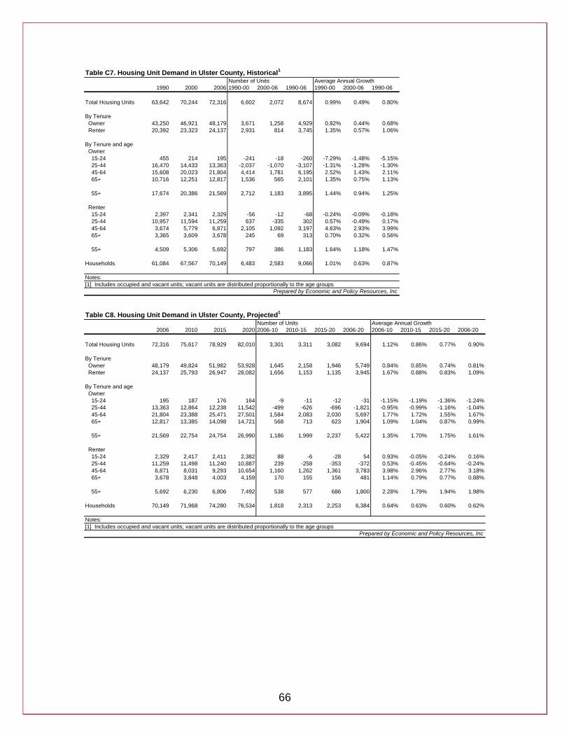
66

Table C7. Housing Unit Demand in Ulster County, Historical1Number of Units Average Annual Growth

1990 2000 2006 1990-00 2000-06 1990-06 1990-00 2000-06 1990-06


By Tenure Owner 43,250 46,921 48,179 3,671 1,258 4,929 0.82% 0.44% 0.68% Renter 20,392 23,323 24,137 2,931 814 3,745 1.35% 0.57% 1.06%

By Tenure and age Owner 15-24 455 214 195 -241 -18 -260 -7.29% -1.48% -5.15% 25-44 16,470 14,433 13,363 -2,037 -1,070 -3,107 -1.31% -1.28% -1.30% 45-64 15,608 20,023 21,804 4,414 1,781 6,195 2.52% 1.43% 2.11% 65+ 10,716 12,251 12,817 1,536 565 2,101 1.35% 0.75% 1.13%

55+ 17,674 20,386 21,569 2,712 1,183 3,895 1.44% 0.94% 1.25%

Renter 15-24 2,397 2,341 2,329 -56 -12 -68 -0.24% -0.09% -0.18% 25-44 10,957 11,594 11,259 637 -335 302 0.57% -0.49% 0.17% 45-64 3,674 5,779 6,871 2,105 1,092 3,197 4.63% 2.93% 3.99% 65+ 3,365 3,609 3,678 245 69 313 0.70% 0.32% 0.56%

55+ 4,509 5,306 5,692 797 386 1,183 1.64% 1.18% 1.47%

Households 61,084 67,567 70,149 6,483 2,583 9,066 1.01% 0.63% 0.87%



Table C8. Housing Unit Demand in Ulster County, Projected1




By Tenure and age Owner 15-24 195 187 176 164 -9 -11 -12 -31 -1.15% -1.19% -1.36% -1.24% 25-44 13,363 12,864 12,238 11,542 -499 -626 -696 -1,821 -0.95% -0.99% -1.16% -1.04% 45-64 21,804 23,388 25,471 27,501 1,584 2,083 2,030 5,697 1.77% 1.72% 1.55% 1.67% 65+ 12,817 13,385 14,098 14,721 568 713 623 1,904 1.09% 1.04% 0.87% 0.99%

55+ 21,569 22,754 24,754 26,990 1,186 1,999 2,237 5,422 1.35% 1.70% 1.75% 1.61%

Renter 15-24 2,329 2,417 2,411 2,382 88 -6 -28 54 0.93% -0.05% -0.24% 0.16% 25-44 11,259 11,498 11,240 10,887 239 -258 -353 -372 0.53% -0.45% -0.64% -0.24% 45-64 6,871 8,031 9,293 10,654 1,160 1,262 1,361 3,783 3.98% 2.96% 2.77% 3.18% 65+ 3,678 3,848 4,003 4,159 170 155 156 481 1.14% 0.79% 0.77% 0.88%

55+ 5,692 6,230 6,806 7,492 538 577 686 1,800 2.28% 1.79% 1.94% 1.98%

Households 70,149 71,968 74,280 76,534 1,818 2,313 2,253 6,384 0.64% 0.63% 0.60% 0.62%



67

Appendix D. Affordability Calculations in Detail This appendix describes the methods used to calculate the affordable house price and rent for each of the Counties. The method employed in this study utilizes the overall approach-theory of the U.S. Department of Housing and Urban Development (HUD). This approach states that no household should spend more than 30% of its income on housing costs. If a household spends more than 30% of its income on housing costs, the household is considered housing-cost stressed. This study’s approach builds on the HUD theory to determine “how much house” can be affordably purchased from net household income after paying the costs of utilities and home owner’s insurance, property taxes, and debt service costs on a conventional 30 year-5% down payment mortgage. This study uses an iterative model based on costs per $1,000 in house value. A general description of the method is presented first, followed by additional details for each step in the process. The starting point for the analysis was the estimate of 2006 median household income for each county in the study region. The estimates of 2006 household (HH) income were then segmented into four different groupings consistent with the traditional HUD approach as follows:

o <50% of HH median income o >50% but <80% of HH median income o >80% but <100% of HH median income o >100% but <120% of HH median income

Calculations were made for each of the income groups described above based on the following general assumptions: (1) per the HUD definition, households would spend up to 30% of their household income on housing before feeling housing cost stress and households would spend up to that 30% level of their household income for “affordable payments,” (2) the analysis would use the mortgage interest rate of 6.41% for 2006—consistent with the prevailing 30-year, 5% down payment mortgage rates that were available in the 3 county market area in calendar year 2006,14 (3) that households that own their home would insure their homes at market rates, and (4) that renter households would pay utilities costs of roughly 49% of owner households. The following diagram lays out the step-by-step calculations used for each household income category for owner housing:

14 The average mortgage rate for 2006 is based on the Federal Home Loan Mortgage Corporation (Freddie Mac) weekly surveys of 125 nationwide lenders.

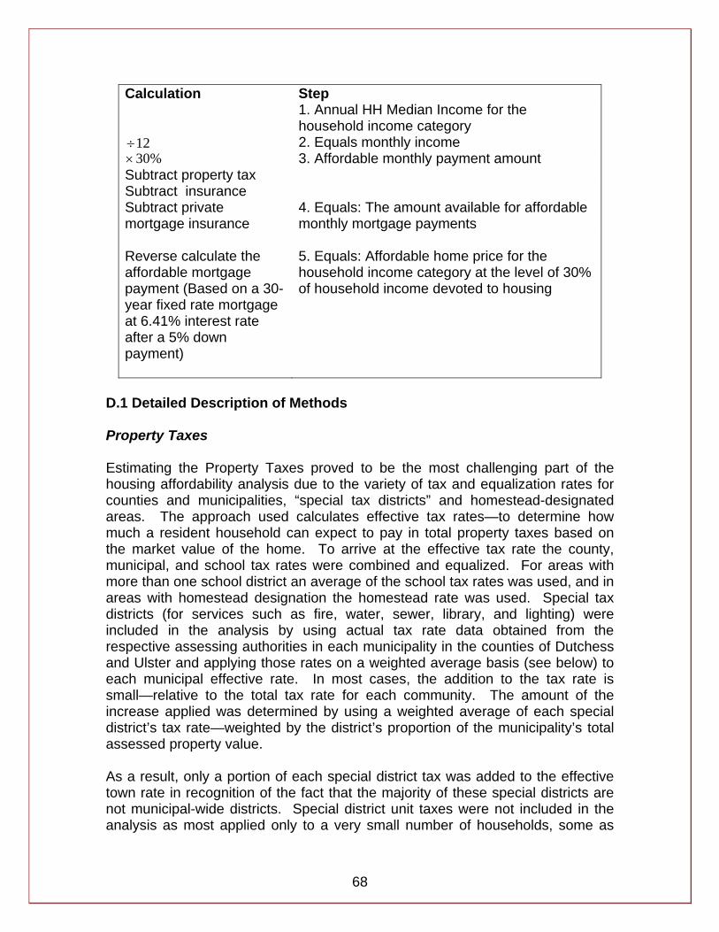
68

Calculation Step 1. Annual HH Median Income for the

household income category 12÷ 2. Equals monthly income

%30× 3. Affordable monthly payment amount Subtract property tax Subtract insurance Subtract private mortgage insurance

4. Equals: The amount available for affordable monthly mortgage payments

Reverse calculate the affordable mortgage payment (Based on a 30- year fixed rate mortgage at 6.41% interest rate after a 5% down payment)

5. Equals: Affordable home price for the household income category at the level of 30% of household income devoted to housing

D.1 Detailed Description of Methods Property Taxes Estimating the Property Taxes proved to be the most challenging part of the housing affordability analysis due to the variety of tax and equalization rates for counties and municipalities, “special tax districts” and homestead-designated areas. The approach used calculates effective tax rates—to determine how much a resident household can expect to pay in total property taxes based on the market value of the home. To arrive at the effective tax rate the county, municipal, and school tax rates were combined and equalized. For areas with more than one school district an average of the school tax rates was used, and in areas with homestead designation the homestead rate was used. Special tax districts (for services such as fire, water, sewer, library, and lighting) were included in the analysis by using actual tax rate data obtained from the respective assessing authorities in each municipality in the counties of Dutchess and Ulster and applying those rates on a weighted average basis (see below) to each municipal effective rate. In most cases, the addition to the tax rate is small—relative to the total tax rate for each community. The amount of the increase applied was determined by using a weighted average of each special district’s tax rate—weighted by the district’s proportion of the municipality’s total assessed property value. As a result, only a portion of each special district tax was added to the effective town rate in recognition of the fact that the majority of these special districts are not municipal-wide districts. Special district unit taxes were not included in the analysis as most applied only to a very small number of households, some as

69

few as 10 households in municipalities with several thousand households. One unit tax was included–a town-wide water tax in the Town of Poughkeepsie in Dutchess County. A total tax of $64 per year per unit was added. Overall, the method results in reasonable effective property tax rates, an average of 2.1% for Dutchess County and 2.5% for Ulster County. The above-described method for incorporating the special tax districts into the analysis was successful for Dutchess and Ulster counties, however it could not be used for Orange County due to lack of available data. As a remedy it was determined that a “sample” of five municipalities in Orange County be taken to represent all the municipalities. The County collected special tax rates from the Towns of Wallkill, New Windsor, Montgomery, Goshen, and Warwick. Based on rates from these towns an assumption was developed that was applied to all towns in the County. This assumption was that special taxes in Orange County add about 0.1% to the estimated effective tax rate at the municipal level and this amount was applied across all municipalities in the County. The results overall appear reasonable, yielding an average effective property tax rate of 2.5% for the county. Homeowners Insurance Costs Homeowner’s insurance costs in the affordability analysis were estimated using 2002 data from the New York State Department of Insurance. The Department provided rates for 25 companies offering home owner’s insurance policies in the counties under study. According to the Department, “Home Owner’s-3” (HO-3) is the most common type of policy purchased and for this reason HO-3 rates were used. Using the rates provided, an average premium was calculated for “Frame Construction” and “Brick Construction” policies. An average of the two types was calculated. This average premium was divided by the median house price for the county, yielding an estimated “cost per $1,000 in housing value.” Finally, because this estimated cost was from calendar year 2002, an insurance CPI15 from the U.S. Department of Labor—Bureau of Labor Statistics was used to convert the 2002 dollar values to 2006 dollars. The result is an estimated cost per $1,000 of value that can be applied to the 2006 housing values which were used in the affordability calculations. Private Mortgage Insurance The affordability calculations assumed a 5% down payment, which requires the cost of private mortgage insurance (PMI) to be included in the analysis. PMI is insurance that protects the lender against default and is usually required when the loan value is 80% or more of the house value (i.e. the down payment is less than 20%). Borrowers continue to pay PMI premiums until the loan value is less than 80% of the value of the house. Lenders usually use third party insurance companies to insure their loans, so rates and approval can vary across 15 CPI means Consumer Price Index—a universally accepted gauge for inflation.

70

companies and depend on many factors such as the value of the loan, the value of the house, type of loan, credit history, and type of property being purchased. While PMI makes it possible to buy a home with less of a down payment, it also represents additional costs to borrowers even though it is insurance that protects the lender. For the purpose of this study PMI rate quotes were obtained from several national companies that offer PMI coverage and cross checked with Ulster Savings Bank.16 Assuming the borrower has a good credit history, will make a 5% down payment and will purchase a single family home to be occupied by the owner, a reasonable PMI rate was estimated to be 0.78%. This rate was multiplied by the amount of the mortgage value to yield an annual PMI premium, and then divided by 12 for the estimated monthly payment. Owner Utility Costs17 Owner utility costs were estimated using consumer expenditure data from the Bureau of Labor Statistics 2002-03 CEX (Consumer Expenditure Survey) for the northeast region of the United States, and data provided by Central Hudson. The CEX survey reported average expenditures on household utilities by income level. Central Hudson Utility provided average expenditures in the 3-County region for 2002, making the analysis more specific to the region, versus the CEX numbers which reflected broader regional averages for the northeastern United States. Using the distribution of the CEX expenditures (less Telephone) for each household income category, the Central Hudson average household bill data was used to calibrate each household income category’s utilities expenditures. New utilities expenditures levels were calculated for each household income category using the Central Hudson average customer bill data. For example, if households in the household income group $30,000-$39,999 spent 17% less than the average on natural gas in the CEX survey, this household income group spent that same proportion less for natural gas, using the Central Hudson bill data as the calibration point. This approach essentially meant that the CEX data was re-calibrated by the Central Hudson average bill data to account for the fact that resident households tend to spend somewhat more for their utilities than the average household in the northeastern United States. The result was that the utility expenditures are more specific to the actual household bills paid for utilities

16 Rates were obtained from AIG United Guaranty, PMI Mortgage Insurance Co., and Mortgage Guaranty Insurance Corp, and cross-checked for reasonableness with project committee member from Ulster Savings Bank. Given the assumptions described above, the committee member agreed that the rate of 0.78% was accurate to use for the study. 17 Following the consensus of the technical review committee, utility costs were not included in the “owner” affordability calculations, but were included in the “renter” calculations because of their significance to renters and that approach is consistent with federal and state renter programs. Utility costs remain as significant cost for owners, even if they are not included in the owner unit calculation in this study.

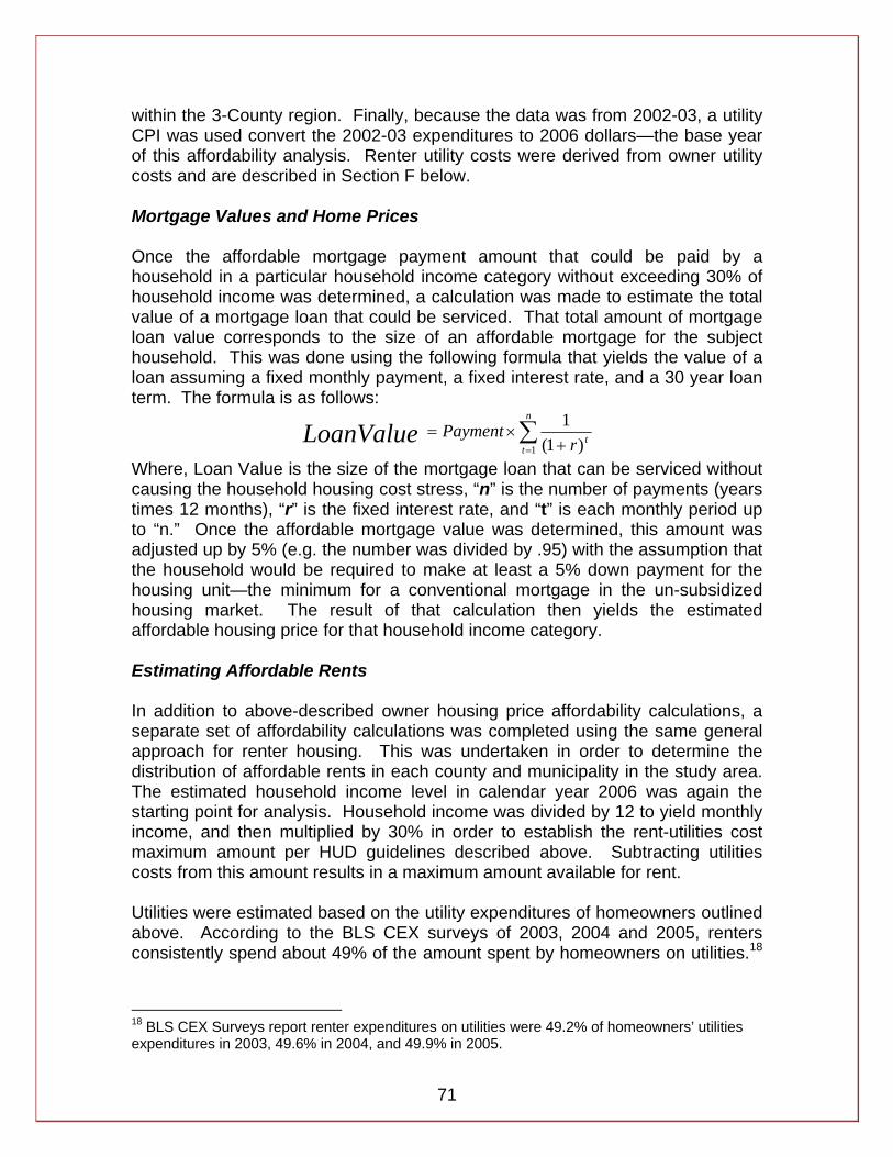
71

within the 3-County region. Finally, because the data was from 2002-03, a utility CPI was used convert the 2002-03 expenditures to 2006 dollars—the base year of this affordability analysis. Renter utility costs were derived from owner utility costs and are described in Section F below. Mortgage Values and Home Prices Once the affordable mortgage payment amount that could be paid by a household in a particular household income category without exceeding 30% of household income was determined, a calculation was made to estimate the total value of a mortgage loan that could be serviced. That total amount of mortgage loan value corresponds to the size of an affordable mortgage for the subject household. This was done using the following formula that yields the value of a loan assuming a fixed monthly payment, a fixed interest rate, and a 30 year loan term. The formula is as follows:

∑= +

×=n

ttr

PaymentLoanValue1 )1(

1

Where, Loan Value is the size of the mortgage loan that can be serviced without causing the household housing cost stress, “n” is the number of payments (years times 12 months), “r” is the fixed interest rate, and “t” is each monthly period up to “n.” Once the affordable mortgage value was determined, this amount was adjusted up by 5% (e.g. the number was divided by .95) with the assumption that the household would be required to make at least a 5% down payment for the housing unit—the minimum for a conventional mortgage in the un-subsidized housing market. The result of that calculation then yields the estimated affordable housing price for that household income category. Estimating Affordable Rents In addition to above-described owner housing price affordability calculations, a separate set of affordability calculations was completed using the same general approach for renter housing. This was undertaken in order to determine the distribution of affordable rents in each county and municipality in the study area. The estimated household income level in calendar year 2006 was again the starting point for analysis. Household income was divided by 12 to yield monthly income, and then multiplied by 30% in order to establish the rent-utilities cost maximum amount per HUD guidelines described above. Subtracting utilities costs from this amount results in a maximum amount available for rent. Utilities were estimated based on the utility expenditures of homeowners outlined above. According to the BLS CEX surveys of 2003, 2004 and 2005, renters consistently spend about 49% of the amount spent by homeowners on utilities.18

18 BLS CEX Surveys report renter expenditures on utilities were 49.2% of homeowners’ utilities expenditures in 2003, 49.6% in 2004, and 49.9% in 2005.

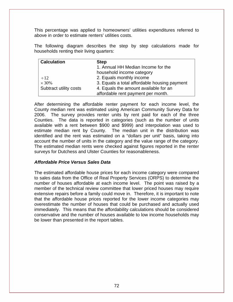
72

This percentage was applied to homeowners’ utilities expenditures referred to above in order to estimate renters’ utilities costs. The following diagram describes the step by step calculations made for households renting their living quarters:

Calculation Step 1. Annual HH Median Income for the

household income category 12÷ 2. Equals monthly income

%30× 3. Equals a total affordable housing payment Subtract utility costs 4. Equals the amount available for an

affordable rent payment per month. After determining the affordable renter payment for each income level, the County median rent was estimated using American Community Survey Data for 2006. The survey provides renter units by rent paid for each of the three Counties. The data is reported in categories (such as the number of units available with a rent between $900 and $999) and interpolation was used to estimate median rent by County. The median unit in the distribution was identified and the rent was estimated on a “dollars per unit” basis, taking into account the number of units in the category and the value range of the category. The estimated median rents were checked against figures reported in the renter surveys for Dutchess and Ulster Counties for reasonableness. Affordable Price Versus Sales Data The estimated affordable house prices for each income category were compared to sales data from the Office of Real Property Services (ORPS) to determine the number of houses affordable at each income level. The point was raised by a member of the technical review committee that lower priced houses may require extensive repairs before a family could move in. Therefore, it is important to note that the affordable house prices reported for the lower income categories may overestimate the number of houses that could be purchased and actually used immediately. This means that the affordability calculations should be considered conservative and the number of houses available to low income households may be lower than presented in the report tables.

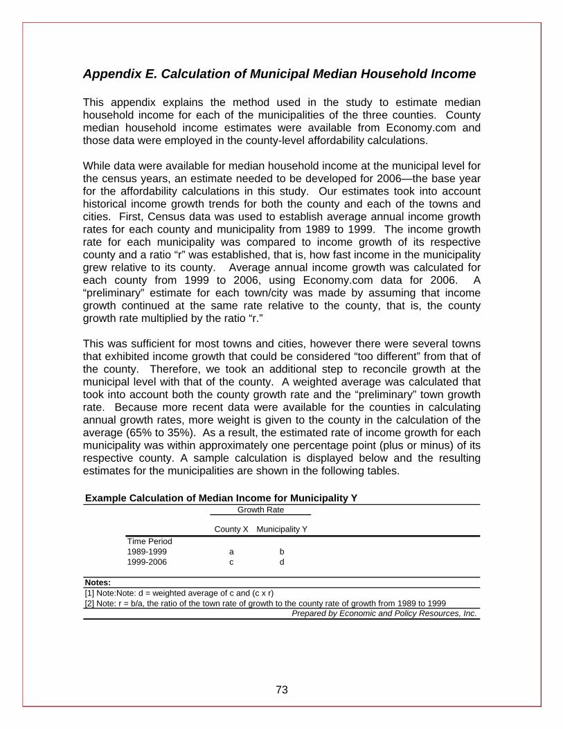
73

Appendix E. Calculation of Municipal Median Household Income This appendix explains the method used in the study to estimate median household income for each of the municipalities of the three counties. County median household income estimates were available from Economy.com and those data were employed in the county-level affordability calculations. While data were available for median household income at the municipal level for the census years, an estimate needed to be developed for 2006—the base year for the affordability calculations in this study. Our estimates took into account historical income growth trends for both the county and each of the towns and cities. First, Census data was used to establish average annual income growth rates for each county and municipality from 1989 to 1999. The income growth rate for each municipality was compared to income growth of its respective county and a ratio “r” was established, that is, how fast income in the municipality grew relative to its county. Average annual income growth was calculated for each county from 1999 to 2006, using Economy.com data for 2006. A “preliminary” estimate for each town/city was made by assuming that income growth continued at the same rate relative to the county, that is, the county growth rate multiplied by the ratio “r.” This was sufficient for most towns and cities, however there were several towns that exhibited income growth that could be considered “too different” from that of the county. Therefore, we took an additional step to reconcile growth at the municipal level with that of the county. A weighted average was calculated that took into account both the county growth rate and the “preliminary” town growth rate. Because more recent data were available for the counties in calculating annual growth rates, more weight is given to the county in the calculation of the average (65% to 35%). As a result, the estimated rate of income growth for each municipality was within approximately one percentage point (plus or minus) of its respective county. A sample calculation is displayed below and the resulting estimates for the municipalities are shown in the following tables. Example Calculation of Median Income for Municipality Y

County X Municipality YTime Period1989-1999 a b1999-2006 c d

Notes:[1] Note:Note: d = weighted average of c and (c x r)[2] Note: r = b/a, the ratio of the town rate of growth to the county rate of growth from 1989 to 1999


Growth Rate

74

Table E1. Median Household Income, Dutchess County

1989[1] 1999[1] 2006[2] 1989-99 1999-06

County 42,250 53,086 66,668 2.3% 3.3%

Municipality Amenia, Town of 31,136 39,231 49,320 2.3% 3.3% Beacon, City of 32,633 45,236 58,789 3.3% 3.8% Beekman, Town of 53,081 65,610 81,923 2.1% 3.2% Clinton, Town of 47,656 66,406 86,448 3.4% 3.8% Dover, Town of 37,376 50,361 64,810 3.0% 3.7% East Fishkill, Town of 54,510 78,394 103,197 3.7% 4.0% Fishkill, Town of 42,711 52,745 65,837 2.1% 3.2% Hyde Park, Town of 44,064 50,870 62,043 1.4% 2.9% La Grange, Town of 53,859 74,881 97,414 3.4% 3.8% Milan, Town of 35,643 54,491 73,295 4.3% 4.3% North East, Town of 30,290 42,038 54,651 3.3% 3.8% Pawling, Town of 47,782 61,380 77,690 2.5% 3.4% Pine Plains, Town of 33,259 43,125 54,751 2.6% 3.5% Pleasant Valley, Town of 42,238 54,578 69,221 2.6% 3.5% Poughkeepsie, City of 27,606 29,389 34,853 0.6% 2.5% Poughkeepsie, Town of 45,886 55,327 68,499 1.9% 3.1% Red Hook, Town of 38,716 46,701 57,819 1.9% 3.1% Rhinebeck, Town of 37,235 52,679 68,949 3.5% 3.9% Stanford, Town of 41,635 54,118 68,778 2.7% 3.5% Union Vale, Town of 51,283 70,500 91,344 3.2% 3.8% Wappinger, Town of 48,659 58,078 71,661 1.8% 3.0% Washington, Town of 41,368 52,104 65,481 2.3% 3.3%

Notes:[1] Note: Source for 1989 and 1999 is U.S. Census[2] Note: 2006 Municipality estimates from EPR; County estimate from Moody's Economy.com


Average Annual Growth

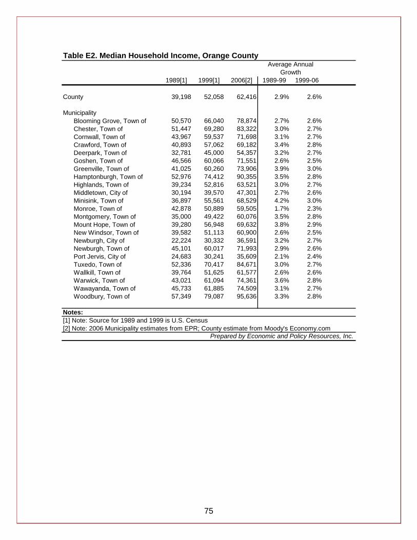
75

Table E2. Median Household Income, Orange County

1989[1] 1999[1] 2006[2] 1989-99 1999-06

County 39,198 52,058 62,416 2.9% 2.6%

Municipality Blooming Grove, Town of 50,570 66,040 78,874 2.7% 2.6% Chester, Town of 51,447 69,280 83,322 3.0% 2.7% Cornwall, Town of 43,967 59,537 71,698 3.1% 2.7% Crawford, Town of 40,893 57,062 69,182 3.4% 2.8% Deerpark, Town of 32,781 45,000 54,357 3.2% 2.7% Goshen, Town of 46,566 60,066 71,551 2.6% 2.5% Greenville, Town of 41,025 60,260 73,906 3.9% 3.0% Hamptonburgh, Town of 52,976 74,412 90,355 3.5% 2.8% Highlands, Town of 39,234 52,816 63,521 3.0% 2.7% Middletown, City of 30,194 39,570 47,301 2.7% 2.6% Minisink, Town of 36,897 55,561 68,529 4.2% 3.0% Monroe, Town of 42,878 50,889 59,505 1.7% 2.3% Montgomery, Town of 35,000 49,422 60,076 3.5% 2.8% Mount Hope, Town of 39,280 56,948 69,632 3.8% 2.9% New Windsor, Town of 39,582 51,113 60,900 2.6% 2.5% Newburgh, City of 22,224 30,332 36,591 3.2% 2.7% Newburgh, Town of 45,101 60,017 71,993 2.9% 2.6% Port Jervis, City of 24,683 30,241 35,609 2.1% 2.4% Tuxedo, Town of 52,336 70,417 84,671 3.0% 2.7% Wallkill, Town of 39,764 51,625 61,577 2.6% 2.6% Warwick, Town of 43,021 61,094 74,361 3.6% 2.8% Wawayanda, Town of 45,733 61,885 74,509 3.1% 2.7% Woodbury, Town of 57,349 79,087 95,636 3.3% 2.8%




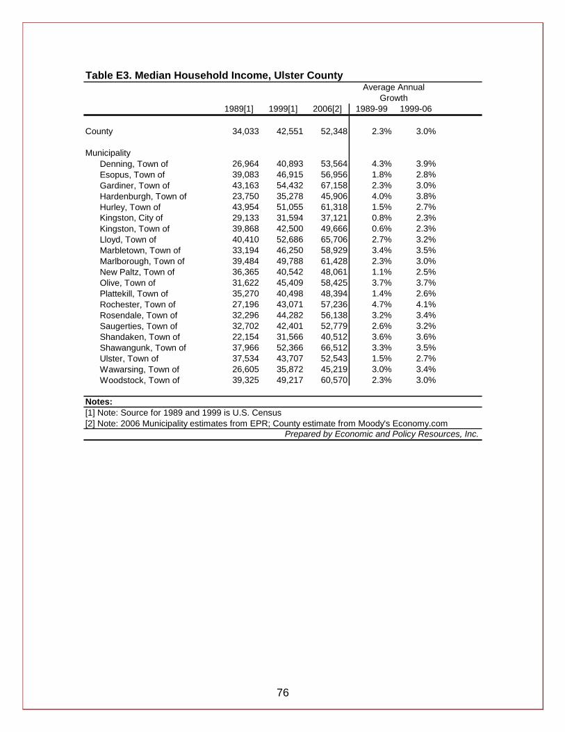
76

Table E3. Median Household Income, Ulster County

1989[1] 1999[1] 2006[2] 1989-99 1999-06

County 34,033 42,551 52,348 2.3% 3.0%

Municipality Denning, Town of 26,964 40,893 53,564 4.3% 3.9% Esopus, Town of 39,083 46,915 56,956 1.8% 2.8% Gardiner, Town of 43,163 54,432 67,158 2.3% 3.0% Hardenburgh, Town of 23,750 35,278 45,906 4.0% 3.8% Hurley, Town of 43,954 51,055 61,318 1.5% 2.7% Kingston, City of 29,133 31,594 37,121 0.8% 2.3% Kingston, Town of 39,868 42,500 49,666 0.6% 2.3% Lloyd, Town of 40,410 52,686 65,706 2.7% 3.2% Marbletown, Town of 33,194 46,250 58,929 3.4% 3.5% Marlborough, Town of 39,484 49,788 61,428 2.3% 3.0% New Paltz, Town of 36,365 40,542 48,061 1.1% 2.5% Olive, Town of 31,622 45,409 58,425 3.7% 3.7% Plattekill, Town of 35,270 40,498 48,394 1.4% 2.6% Rochester, Town of 27,196 43,071 57,236 4.7% 4.1% Rosendale, Town of 32,296 44,282 56,138 3.2% 3.4% Saugerties, Town of 32,702 42,401 52,779 2.6% 3.2% Shandaken, Town of 22,154 31,566 40,512 3.6% 3.6% Shawangunk, Town of 37,966 52,366 66,512 3.3% 3.5% Ulster, Town of 37,534 43,707 52,543 1.5% 2.7% Wawarsing, Town of 26,605 35,872 45,219 3.0% 3.4% Woodstock, Town of 39,325 49,217 60,570 2.3% 3.0%




77

Appendix F. Municipal Allocations This appendix describes the methods used to determine each municipality’s proportion of the 2006 estimated county affordability gap. The municipal allocations were developed after full investigation of a number of alternative methodologies. More than a dozen allocation factors were studied and applied. The Planning Department staffs and the full project Steering Committee examined and commented on several versions of these municipal allocations. Final versions of these allocations included the effect of what was determined to be a structural change in the energy price environment from a period of relatively inexpensive oil and gasoline to a period of elevated energy prices. Planning Department staff and the Project Steering Committee agreed that the changed energy price environment is likely to endure throughout the study’s time horizon or through calendar year 2020. Staff and the Project Steering Committee indicated that this situation, along with consideration of on-going county development policies to encourage future growth toward appropriate places in each county should be included in the allocations methodology for each respective county. These factors were incorporated via a “development capability factor,” which was used as an indication of where future development is likely to occur due to the reality of increased energy prices and the stated development policies of all three County Planning Boards. The development capability factors assigned each municipality to a category, indicating the municipality’s capability for compact development, taking into account existing infrastructure (e.g. sewer and potable water capacity, transportation (e.g. transit) capacity, landscape conditions, past development (e.g. existence of villages) and others as determined by each county Planning Board staff. The municipalities were categorized into groups and received points as follows:

1 = “not capable of compact development” (generally the rural areas), 3 = “low capacity for compact development” (some suburban areas), 5 = “medium capacity for compact development” (some suburban areas), 10 = “already has compact development and/or has significant capacity for compact development” (generally the urban areas or municipalities with existing villages).

The “development capability factor” was incorporated with other variables that influence affordability issues, such as income, tax rates, poverty rates, and price growth relative to income growth, through a series of weighted indexes. Weights were assigned as follows:

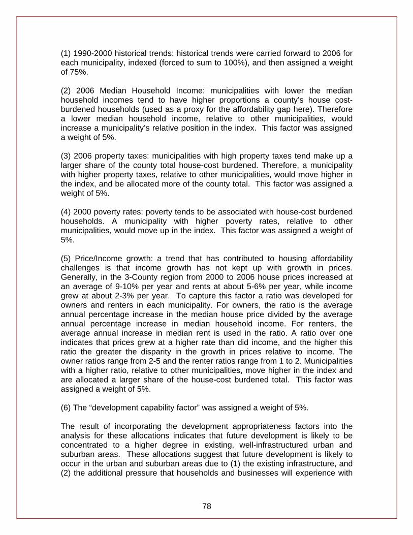
78

(1) 1990-2000 historical trends: historical trends were carried forward to 2006 for each municipality, indexed (forced to sum to 100%), and then assigned a weight of 75%. (2) 2006 Median Household Income: municipalities with lower the median household incomes tend to have higher proportions a county’s house cost-burdened households (used as a proxy for the affordability gap here). Therefore a lower median household income, relative to other municipalities, would increase a municipality’s relative position in the index. This factor was assigned a weight of 5%. (3) 2006 property taxes: municipalities with high property taxes tend make up a larger share of the county total house-cost burdened. Therefore, a municipality with higher property taxes, relative to other municipalities, would move higher in the index, and be allocated more of the county total. This factor was assigned a weight of 5%. (4) 2000 poverty rates: poverty tends to be associated with house-cost burdened households. A municipality with higher poverty rates, relative to other municipalities, would move up in the index. This factor was assigned a weight of 5%. (5) Price/Income growth: a trend that has contributed to housing affordability challenges is that income growth has not kept up with growth in prices. Generally, in the 3-County region from 2000 to 2006 house prices increased at an average of 9-10% per year and rents at about 5-6% per year, while income grew at about 2-3% per year. To capture this factor a ratio was developed for owners and renters in each municipality. For owners, the ratio is the average annual percentage increase in the median house price divided by the average annual percentage increase in median household income. For renters, the average annual increase in median rent is used in the ratio. A ratio over one indicates that prices grew at a higher rate than did income, and the higher this ratio the greater the disparity in the growth in prices relative to income. The owner ratios range from 2-5 and the renter ratios range from 1 to 2. Municipalities with a higher ratio, relative to other municipalities, move higher in the index and are allocated a larger share of the house-cost burdened total. This factor was assigned a weight of 5%. (6) The “development capability factor” was assigned a weight of 5%. The result of incorporating the development appropriateness factors into the analysis for these allocations indicates that future development is likely to be concentrated to a higher degree in existing, well-infrastructured urban and suburban areas. These allocations suggest that future development is likely to occur in the urban and suburban areas due to (1) the existing infrastructure, and (2) the additional pressure that households and businesses will experience with

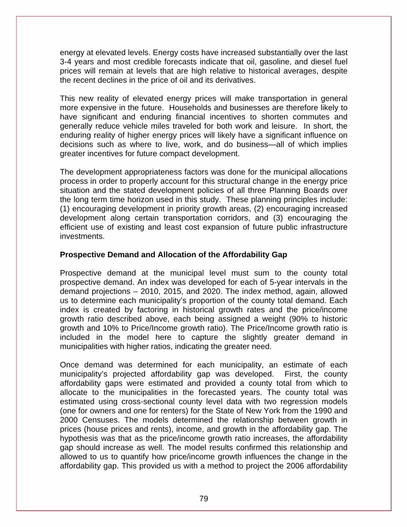
79

energy at elevated levels. Energy costs have increased substantially over the last 3-4 years and most credible forecasts indicate that oil, gasoline, and diesel fuel prices will remain at levels that are high relative to historical averages, despite the recent declines in the price of oil and its derivatives. This new reality of elevated energy prices will make transportation in general more expensive in the future. Households and businesses are therefore likely to have significant and enduring financial incentives to shorten commutes and generally reduce vehicle miles traveled for both work and leisure. In short, the enduring reality of higher energy prices will likely have a significant influence on decisions such as where to live, work, and do business—all of which implies greater incentives for future compact development. The development appropriateness factors was done for the municipal allocations process in order to properly account for this structural change in the energy price situation and the stated development policies of all three Planning Boards over the long term time horizon used in this study. These planning principles include: (1) encouraging development in priority growth areas, (2) encouraging increased development along certain transportation corridors, and (3) encouraging the efficient use of existing and least cost expansion of future public infrastructure investments. Prospective Demand and Allocation of the Affordability Gap Prospective demand at the municipal level must sum to the county total prospective demand. An index was developed for each of 5-year intervals in the demand projections – 2010, 2015, and 2020. The index method, again, allowed us to determine each municipality’s proportion of the county total demand. Each index is created by factoring in historical growth rates and the price/income growth ratio described above, each being assigned a weight (90% to historic growth and 10% to Price/Income growth ratio). The Price/Income growth ratio is included in the model here to capture the slightly greater demand in municipalities with higher ratios, indicating the greater need. Once demand was determined for each municipality, an estimate of each municipality’s projected affordability gap was developed. First, the county affordability gaps were estimated and provided a county total from which to allocate to the municipalities in the forecasted years. The county total was estimated using cross-sectional county level data with two regression models (one for owners and one for renters) for the State of New York from the 1990 and 2000 Censuses. The models determined the relationship between growth in prices (house prices and rents), income, and growth in the affordability gap. The hypothesis was that as the price/income growth ratio increases, the affordability gap should increase as well. The model results confirmed this relationship and allowed to us to quantify how price/income growth influences the change in the affordability gap. This provided us with a method to project the 2006 affordability

80

gap forward to 2020 using forecasts of prices and income previously presented in the economic and demographic forecast. The forecasted county level affordability gap was then allocated to the municipalities based on 1990-2006 trends. Constraints and Opportunities Analysis The municipal allocations were complemented with a constraints and opportunities analysis completed by the County Planning Departments. The analysis was designed to serve as a check for the statistical models of the municipal allocation process – essentially to ensure that the models were appropriately allocating the county total figures. The constraints and opportunities analysis identified natural resource, infrastructure and regulatory characteristics of municipalities that would likely constrain future development, such as steep slopes, lack of water and sewer services and facilities, or regulations and policies that were not conducive to housing development. The analysis also identified municipalities that would be likely to host additional development, based on available developable land, housing development-friendly policies, and local government openness and commitment to building additional housing units. Overall, the constraints and opportunities analysis was a qualitative “reality check” on the quantitative estimates developed in the municipal allocation process.

81

Appendix G. Housing Wage Analysis This supplemental analysis connects the abstract concept of housing affordability to the region’s labor market. In order to accomplish this, earnings in selected job sectors in the 3-County region are compared to the earnings necessary to affordably own a median-priced house, or pay rent on a two bedroom apartment. Data from the Bureau of Labor Statistics’ Quarterly Census of Employment and Wages are used in the analysis. This data set allows for comparison between the average earnings in the top sectors of the regional labor market (as measured by the sector’s share of total employment) and the income necessary to avoid being house cost-burdened. The New York Department of Labor, in cooperation with the U.S. Bureau of Labor Statistics, conducts the QCEW census every quarter for employers “covered” under the state’s unemployment insurance program (UI). The QCEW is part of the quarterly UI filing by employers and requires employers report the number of employees and the total wages paid during the preceding quarter. The data used in assessment is for 2006, and wage figures used are the average of total wages paid from the lowest to the highest paid workers in each sector. Relating Earnings to Housing Affordability Housing affordability is typically measured by the proportion of income used for the cost of housing - if more than 30% of a household’s income goes to costs associated with housing the household is deemed “house cost burdened”. For home owners, the gap between income and home prices is typically measured by comparing household income needed to afford a median priced home without exceeding the 30% housing cost stress threshold. This study relates QCEW wage estimates to typical mortgage payments in the 3 counties. For renters, this analysis focuses on average wages paid to workers by sector in comparison to the median rent for a two bedroom unit in Dutchess, Orange, and Ulster counties. The analysis includes a brief household income distribution analysis in order to help the reader keep the housing wage in perspective. The housing wage concept is useful for assessing the potential for a single earner household to be housing cost burdened. Because today’s economy typically includes many households with more than one earner (e.g. working parents), a straight housing wage comparison is in many ways a worst-case housing affordability scenario. As a result, this study uses earnings multiples for sector-by-sector comparison purposes.19 Defining the Housing Wage

19 Earnings multiple refers to the number of wage earners that would be needed for a household to affordably purchase a median priced house (or the median rent for a two-bedroom apartment).

82

The housing wage figure used in the analysis for owners is the amount of household income per year required to afford a median priced house in each of three counties divided by 2,080 work hours per year (40 hour work week times 52 weeks per year). The amount is calculated using the same set of assumptions described in the affordability calculation section of this report (Section 2.1): beginning with a median priced house, we assume a 5% down payment, a fixed rate 30-year mortgage, property taxes, and insurance costs, and arrive at an annual household income. The annual household income is divided by 2080 to calculate an hourly wage. For renters, the housing wage is provided for each county by the National Low Income Housing Coalition (NLIHC). NLIHC computes housing wage figures for various sized apartments at the county level, workers earning above the housing wage are considered able to affordably rent. The two bedroom housing wage is used as the threshold for potential housing burden; this represents the minimum hourly wage a full time worker in a single earner household would need to affordably rent a unit at the median rent level in a given county. While income includes payments from sources other than wages such as capital gains and dividends from equities and other securities, the households of interest in this study (owner and renters with income at 120% of median income or less) receive most of their income from wages. The following section presents the housing wage analyses by county. Dutchess County Owner Housing Wage The gap between the owner housing wage and average wages in Dutchess County indicates that owning a median-priced home is beyond the means of many single earner households, and indeed even many dual earner households. Average wages in all of the top seven sectors fall short of the owner housing wage; it appears that only the highest paid employees in Dutchess County’s major sectors would be able to afford a new mortgage on a median-price house.

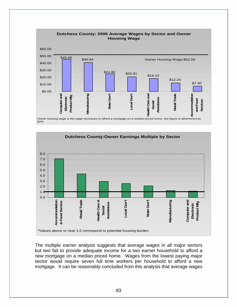
83

Dutchess County: 2006 Average Wages by Sector and Owner Housing Wage

$40.84

$20.81 $18.10$12.24

$7.40

$24.80

$45.65

$0.00

$10.00

$20.00

$30.00

$40.00

$50.00

$60.00

Com

pute

r and

Elec

tron

icPr

oduc

t Mfg

Man

ufac

turin

g

Stat

e G

ov't

Loca

l Gov

't

Hea

lth C

are

and

Soci

alA

ssis

tanc

e

Ret

ail T

rade

Acc

omm

odat

ion

and

Food

Serv

ices

Owner Housing Wage:$52.59

Owner housing wage is the wage necessary to afford a mortgage on a median priced home, this figure is determined by EPR

Dutchess County:Owner Earnings Multiple by Sector

0.0

1.0

2.03.0

4.0

5.0

6.0

7.08.0

Acc

omm

odat

ion

& F

ood

Serv

ice

Ret

ail T

rade

Hea

lth C

are

&So

cial

Ass

ista

nce

Loca

l Gov

't

Stat

e G

ov't

Man

ufac

turin

g

Com

pute

r and

Elec

tron

icPr

oduc

t Mfg

*Values above or near 1.0 correspond to potential housing burden

The multiple earner analysis suggests that average wages in all major sectors but two fail to provide adequate income for a two earner household to afford a new mortgage on a median priced home. Wages from the lowest paying major sector would require seven full time workers per household to afford a new mortgage. It can be reasonably concluded from this analysis that average wages

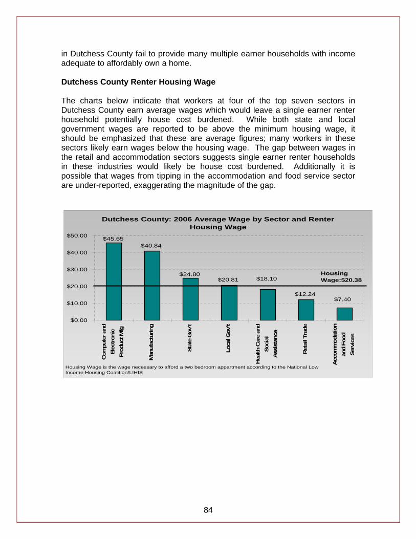
84

in Dutchess County fail to provide many multiple earner households with income adequate to affordably own a home. Dutchess County Renter Housing Wage The charts below indicate that workers at four of the top seven sectors in Dutchess County earn average wages which would leave a single earner renter household potentially house cost burdened. While both state and local government wages are reported to be above the minimum housing wage, it should be emphasized that these are average figures; many workers in these sectors likely earn wages below the housing wage. The gap between wages in the retail and accommodation sectors suggests single earner renter households in these industries would likely be house cost burdened. Additionally it is possible that wages from tipping in the accommodation and food service sector are under-reported, exaggerating the magnitude of the gap.

Dutchess County: 2006 Average Wage by Sector and Renter Housing Wage

$40.84

$20.81

$12.24

$18.10$24.80

$45.65

$7.40

$0.00

$10.00

$20.00

$30.00

$40.00

$50.00

Com

pute

r and

Elec

tron

icPr

oduc

t Mfg

Man

ufac

turin

g

Stat

e G

ov't

Loca

l Gov

't

Hea

lth C

are

and

Soci

alAss

ista

nce

Ret

ail T

rade

Acc

omm

odat

ion

and

Food

Serv

ices

Housing Wage:$20.38

Housing Wage is the wage necessary to afford a two bedroom appartment according to the National Low Income Housing Coalition/LIHIS

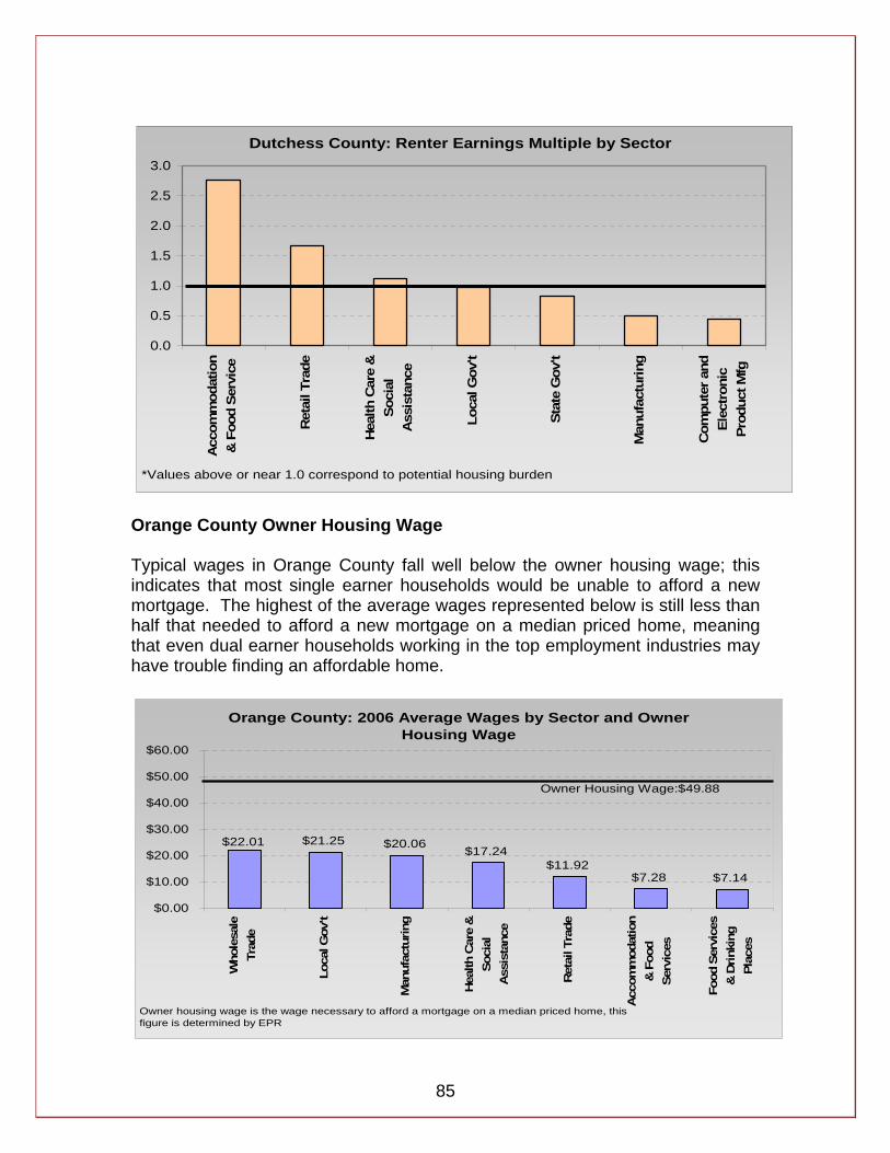
85

Dutchess County: Renter Earnings Multiple by Sector

0.0

0.5

1.0

1.5

2.0

2.5

3.0

Acc

omm

odat

ion

& F

ood

Serv

ice

Ret

ail T

rade

Hea

lth C

are

&So

cial

Ass

ista

nce

Loca

l Gov

't

Stat

e G

ov't

Man

ufac

turin

g

Com

pute

r and

Elec

tron

icPr

oduc

t Mfg


Orange County Owner Housing Wage Typical wages in Orange County fall well below the owner housing wage; this indicates that most single earner households would be unable to afford a new mortgage. The highest of the average wages represented below is still less than half that needed to afford a new mortgage on a median priced home, meaning that even dual earner households working in the top employment industries may have trouble finding an affordable home.

Orange County: 2006 Average Wages by Sector and Owner Housing Wage

$21.25 $20.06 $17.24$11.92

$7.28 $7.14

$22.01

$0.00

$10.00

$20.00

$30.00

$40.00

$50.00

$60.00

Who

lesa

leTr

ade

Loca

l Gov

't

Man

ufac

turin

g

Hea

lth C

are

&So

cial

Ass

ista

nce

Ret

ail T

rade

Acc

omm

odat

ion

& F

ood

Serv

ices

Food

Ser

vice

s&

Drin

king

Plac

es



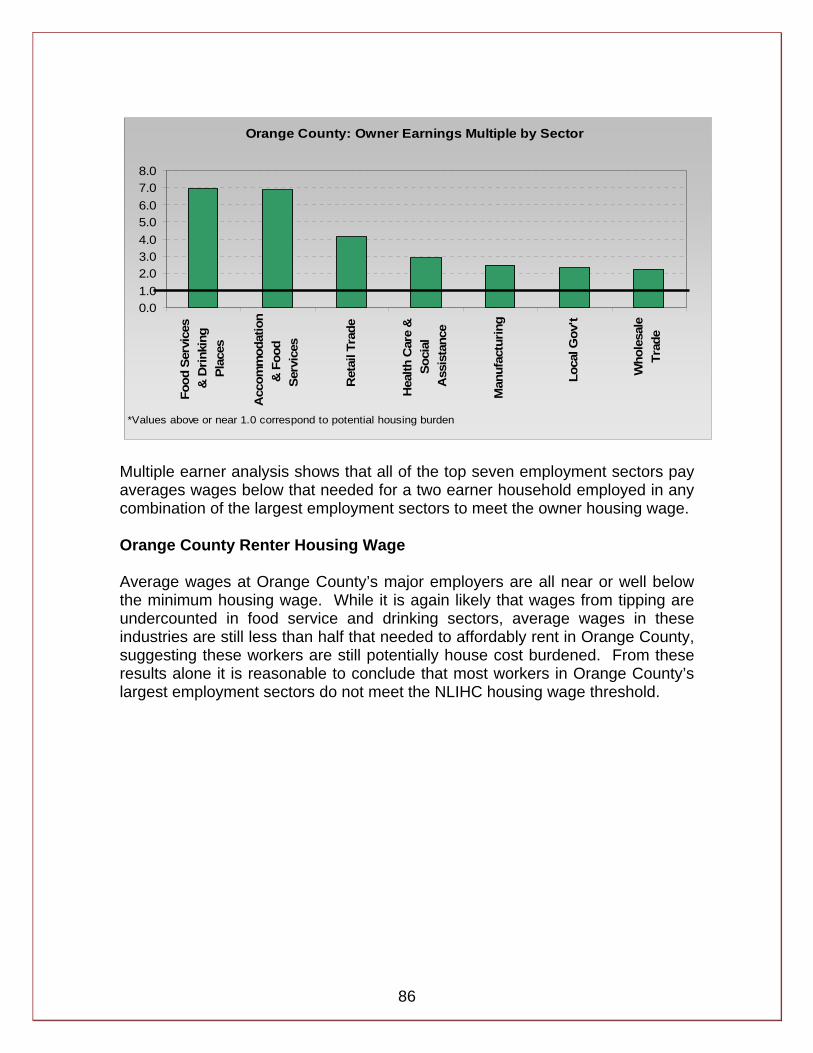
86

Orange County: Owner Earnings Multiple by Sector

0.01.02.03.04.05.06.07.08.0

Food

Ser

vice

s&

Drin

king

Plac

es

Acc

omm

odat

ion

& F

ood

Serv

ices

Ret

ail T

rade

Hea

lth C

are

&So

cial

Ass

ista

nce

Man

ufac

turin

g

Loca

l Gov

't

Who

lesa

leTr

ade


Multiple earner analysis shows that all of the top seven employment sectors pay averages wages below that needed for a two earner household employed in any combination of the largest employment sectors to meet the owner housing wage. Orange County Renter Housing Wage Average wages at Orange County’s major employers are all near or well below the minimum housing wage. While it is again likely that wages from tipping are undercounted in food service and drinking sectors, average wages in these industries are still less than half that needed to affordably rent in Orange County, suggesting these workers are still potentially house cost burdened. From these results alone it is reasonable to conclude that most workers in Orange County’s largest employment sectors do not meet the NLIHC housing wage threshold.

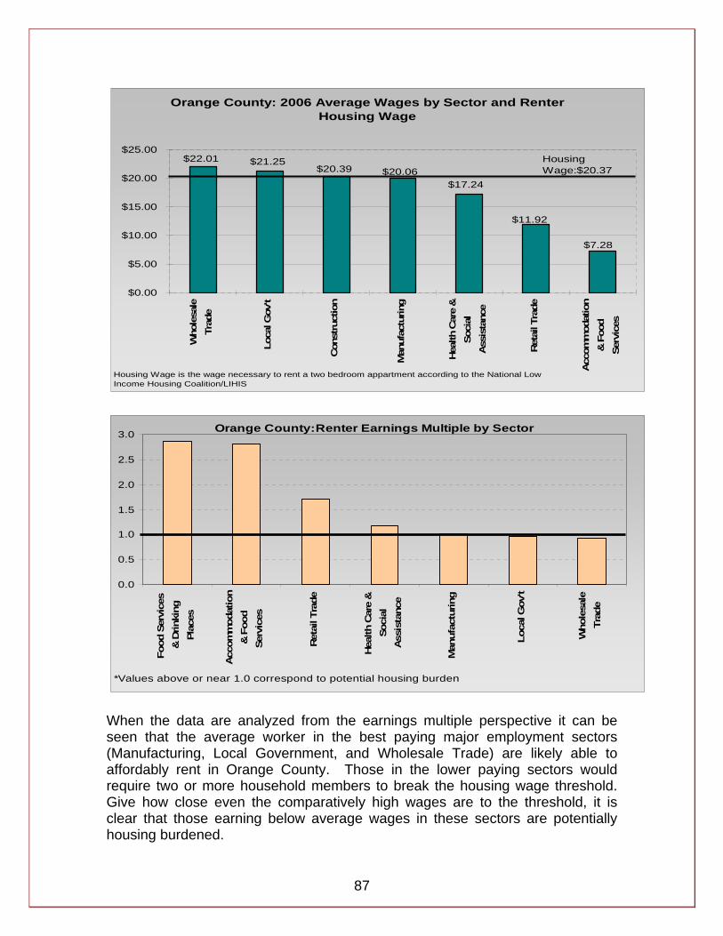
87

Orange County: 2006 Average Wages by Sector and Renter Housing Wage

$21.25

$7.28

$22.01$20.39

$17.24

$11.92

$20.06

$0.00

$5.00

$10.00

$15.00

$20.00

$25.00

Who

lesa

leTr

ade

Loca

l Gov

't

Con

stru

ctio

n

Man

ufac

turin

g

Hea

lth C

are

&So

cial

Ass

ista

nce

Ret

ail T

rade

Acc

omm

odat

ion

& F

ood

Serv

ices

Housing Wage:$20.37

Housing Wage is the wage necessary to rent a two bedroom appartment according to the National Low Income Housing Coalition/LIHIS

Orange County:Renter Earnings Multiple by Sector

0.0

0.5

1.0

1.5

2.0

2.5

3.0

Food

Ser

vice

s&

Drin

king

Plac

es

Acc

omm

odat

ion

& F

ood

Serv

ices

Ret

ail T

rade

Hea

lth C

are

&So

cial

Ass

ista

nce

Man

ufac

turin

g

Loca

l Gov

't

Who

lesa

leTr

ade


When the data are analyzed from the earnings multiple perspective it can be seen that the average worker in the best paying major employment sectors (Manufacturing, Local Government, and Wholesale Trade) are likely able to affordably rent in Orange County. Those in the lower paying sectors would require two or more household members to break the housing wage threshold. Give how close even the comparatively high wages are to the threshold, it is clear that those earning below average wages in these sectors are potentially housing burdened.

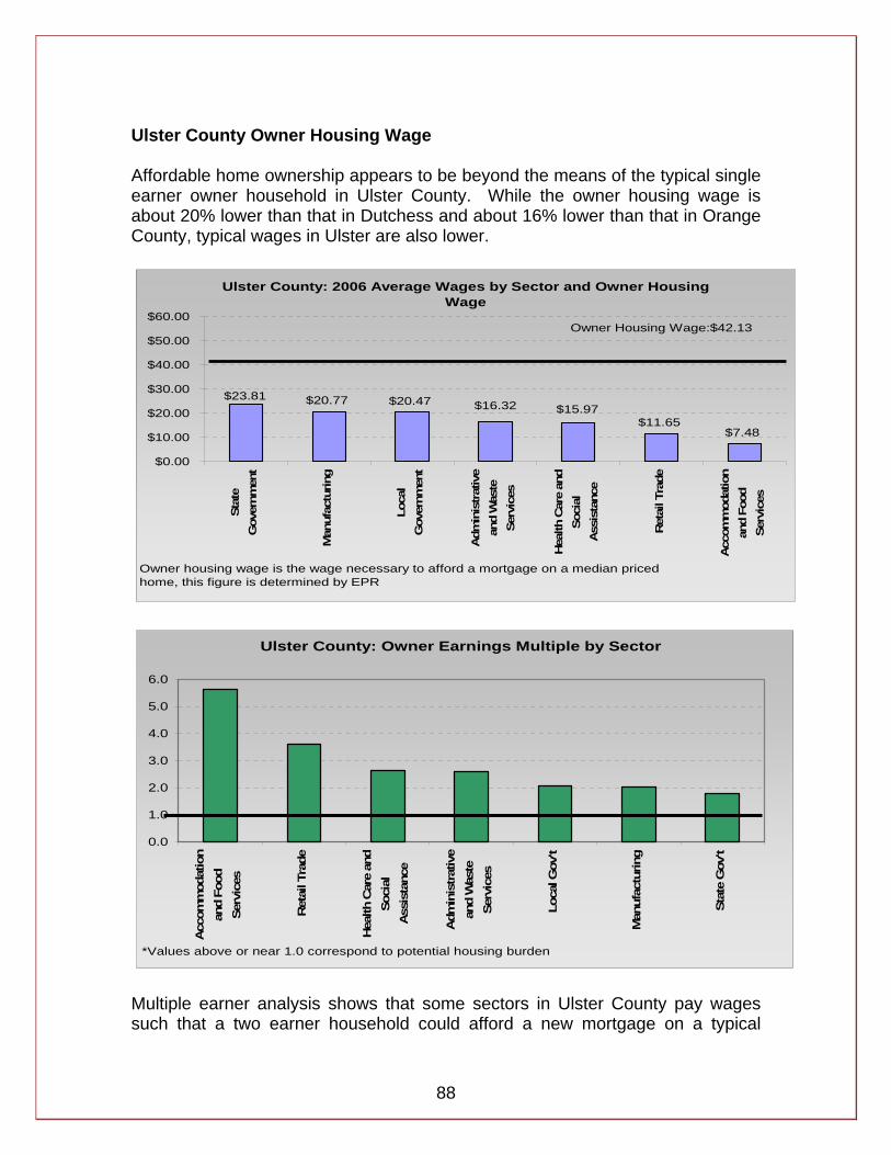
88

Ulster County Owner Housing Wage Affordable home ownership appears to be beyond the means of the typical single earner owner household in Ulster County. While the owner housing wage is about 20% lower than that in Dutchess and about 16% lower than that in Orange County, typical wages in Ulster are also lower.

Ulster County: 2006 Average Wages by Sector and Owner Housing Wage

$20.77 $20.47

$11.65$7.48

$16.32 $15.97$23.81

$0.00

$10.00

$20.00

$30.00

$40.00

$50.00

$60.00

Stat

eG

over

nmen

t

Man

ufac

turin

g

Loca

lG

over

nmen

t

Adm

inis

trat

ive

and

Was

teSe

rvic

es

Hea

lth C

are

and

Soci

alA

ssis

tanc

e

Ret

ail T

rade

Acc

omm

odat

ion

and

Food

Serv

ices



Ulster County: Owner Earnings Multiple by Sector

0.0

1.0

2.0

3.0

4.0

5.0

6.0

Acc

omm

odat

ion

and

Food

Serv

ices

Ret

ail T

rade

Hea

lth C

are

and

Soci

alA

ssis

tanc

e

Adm

inis

trat

ive

and

Was

teSe

rvic

es

Loca

l Gov

't

Man

ufac

turin

g

Stat

e G

ov't


Multiple earner analysis shows that some sectors in Ulster County pay wages such that a two earner household could afford a new mortgage on a typical

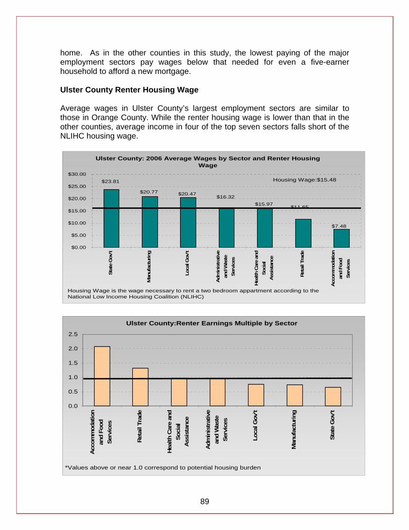
89

home. As in the other counties in this study, the lowest paying of the major employment sectors pay wages below that needed for even a five-earner household to afford a new mortgage. Ulster County Renter Housing Wage Average wages in Ulster County’s largest employment sectors are similar to those in Orange County. While the renter housing wage is lower than that in the other counties, average income in four of the top seven sectors falls short of the NLIHC housing wage.

Ulster County: 2006 Average Wages by Sector and Renter Housing Wage

$20.77$16.32

$11.65$15.97

$20.47

$23.81

$7.48

$0.00

$5.00

$10.00

$15.00

$20.00

$25.00

$30.00

Stat

e G

ov't

Man

ufac

turin

g

Loca

l Gov

't

Adm

inis

trat

ive

and

Was

teSe

rvic

es

Hea

lth C

are

and

Soci

alA

ssis

tanc

e

Ret

ail T

rade

Acc

omm

odat

ion

and

Food

Serv

ices

Housing Wage:$15.48

Housing Wage is the wage necessary to rent a two bedroom appartment according to the National Low Income Housing Coalition (NLIHC)

Ulster County:Renter Earnings Multiple by Sector

0.0

0.5

1.0

1.5

2.0

2.5

Acc

omm

odat

ion

and

Food

Serv

ices

Ret

ail T

rade

Hea

lth C

are

and

Soci

alA

ssis

tanc

e

Adm

inis

trat

ive

and

Was

teSe

rvic

es

Loca

l Gov

't

Man

ufac

turin

g

Stat

e G

ov't


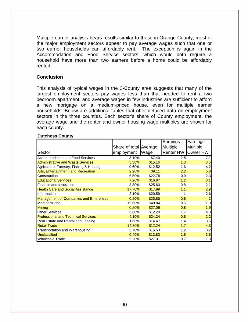
90

Multiple earner analysis bears results similar to those in Orange County, most of the major employment sectors appear to pay average wages such that one or two earner households can affordably rent. The exception is again in the Accommodation and Food Service sectors, which would both require a household have more than two earners before a home could be affordably rented. Conclusion This analysis of typical wages in the 3-County area suggests that many of the largest employment sectors pay wages less than that needed to rent a two bedroom apartment, and average wages in few industries are sufficient to afford a new mortgage on a medium-priced house, even for multiple earner households. Below are additional tables that offer detailed data on employment sectors in the three counties. Each sector’s share of County employment, the average wage and the renter and owner housing wage multiples are shown for each county.

Dutchess County

SectorShare of total employment

Average Wage

Earnings Multiple Renter HW

Earnings Multiple Owner HW

Accommodation and Food Services 8.10% $7.40 2.8 7.1Administrative and Waste Services 5.50% $15.16 1.3 3.5Agriculture, Forestry, Fishing & Hunting 0.60% $12.52 1.6 4.2Arts, Entertainment, and Recreation 2.20% $9.11 2.2 5.8Construction 6.50% $22.78 0.9 2.3Educational Services 7.20% $16.87 1.2 3.1Finance and Insurance 3.30% $25.60 0.8 2.1Health Care and Social Assistance 17.70% $17.99 1.1 2.9Information 2.10% $20.59 1 2.6Management of Companies and Enterprises 0.80% $25.86 0.8 2Manufacturing 15.60% $40.84 0.5 1.3Mining 0.20% $27.06 0.8 1.9Other Services 3.60% $12.20 1.7 4.3Professional and Technical Services 4.10% $24.24 0.8 2.2Real Estate and Rental and Leasing 1.60% $14.47 1.4 3.6Retail Trade 14.80% $12.24 1.7 4.3Transportation and Warehousing 3.70% $16.53 1.2 3.2Unclassified 0.40% $13.83 1.5 3.8Wholesale Trade 2.20% $27.31 0.7 1.9

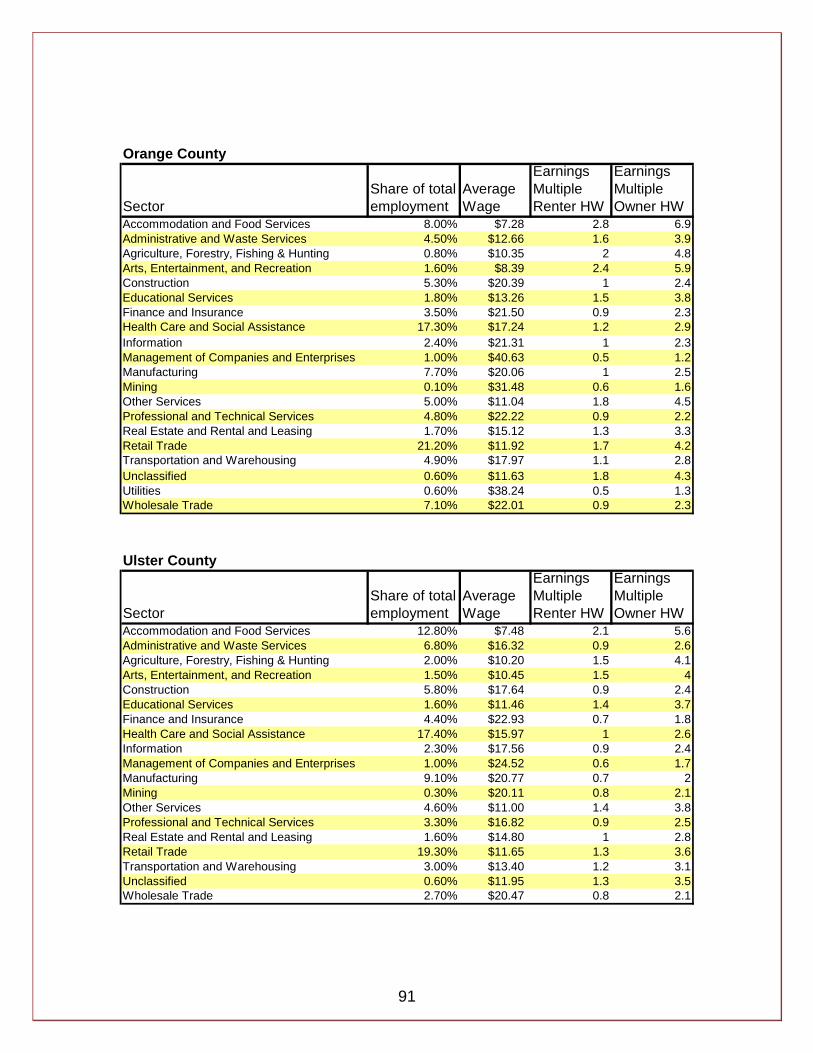
91

Orange County


Average Wage



Accommodation and Food Services 8.00% $7.28 2.8 6.9Administrative and Waste Services 4.50% $12.66 1.6 3.9Agriculture, Forestry, Fishing & Hunting 0.80% $10.35 2 4.8Arts, Entertainment, and Recreation 1.60% $8.39 2.4 5.9Construction 5.30% $20.39 1 2.4Educational Services 1.80% $13.26 1.5 3.8Finance and Insurance 3.50% $21.50 0.9 2.3Health Care and Social Assistance 17.30% $17.24 1.2 2.9Information 2.40% $21.31 1 2.3Management of Companies and Enterprises 1.00% $40.63 0.5 1.2Manufacturing 7.70% $20.06 1 2.5Mining 0.10% $31.48 0.6 1.6Other Services 5.00% $11.04 1.8 4.5Professional and Technical Services 4.80% $22.22 0.9 2.2Real Estate and Rental and Leasing 1.70% $15.12 1.3 3.3Retail Trade 21.20% $11.92 1.7 4.2Transportation and Warehousing 4.90% $17.97 1.1 2.8Unclassified 0.60% $11.63 1.8 4.3Utilities 0.60% $38.24 0.5 1.3Wholesale Trade 7.10% $22.01 0.9 2.3 Ulster County


Average Wage



Accommodation and Food Services 12.80% $7.48 2.1 5.6Administrative and Waste Services 6.80% $16.32 0.9 2.6Agriculture, Forestry, Fishing & Hunting 2.00% $10.20 1.5 4.1Arts, Entertainment, and Recreation 1.50% $10.45 1.5 4Construction 5.80% $17.64 0.9 2.4Educational Services 1.60% $11.46 1.4 3.7Finance and Insurance 4.40% $22.93 0.7 1.8Health Care and Social Assistance 17.40% $15.97 1 2.6Information 2.30% $17.56 0.9 2.4Management of Companies and Enterprises 1.00% $24.52 0.6 1.7Manufacturing 9.10% $20.77 0.7 2Mining 0.30% $20.11 0.8 2.1Other Services 4.60% $11.00 1.4 3.8Professional and Technical Services 3.30% $16.82 0.9 2.5Real Estate and Rental and Leasing 1.60% $14.80 1 2.8Retail Trade 19.30% $11.65 1.3 3.6Transportation and Warehousing 3.00% $13.40 1.2 3.1Unclassified 0.60% $11.95 1.3 3.5Wholesale Trade 2.70% $20.47 0.8 2.1

92

Appendix H. SWOT Analysis: Strengths, Weaknesses, Opportunities, and Threats for the 3-County Region As part of this Regional Housing Needs Assessment, a Strengths, Weaknesses, Opportunities, and Threats assessment (or what is commonly known as a SWOT) was conducted. Key regional stakeholders active in housing issues were identified in each county by the respective County Planning Departments. The interviews were conducted during late October-early November 2007. Those selected for interviews involved a broad range of participants in the regional housing arena including local government officials, non profit administrators, and private developers. The objectives of these interviews were: (1) to obtain a “reality check” on the data our analysis team had assembled to date, (2) to get a face to face description of the facts and nuances of the situation “on the ground” including any possible constraints and/or opportunities, (3) to identify what stakeholders view as notable constraints to housing development in the region, and (4) to solicit ideas and insights which might lead to solutions to the housing market issues and identify housing market opportunities that could be of use to stakeholders in the deliberations that are likely to follow the completion of this housing needs assessment. While there are many findings of note in this SWOT analysis, one general finding came clearly through from the interview process. SWOT respondents in various ways indicated that although the three County governments, several competent non-profit agencies and a handful of private developers understand the problem and are willing to take action, only a scattering of municipalities outside of the region’s cities have shown a willingness to undertake necessary actions to address the region’s housing challenges. This condition will likely act as a general impediment to the development of housing in at least parts of the 3 county region. The final part of this SOWT assessment included the development of an inventory of ideas from stakeholders that could be used to jumpstart the development of an action agenda. Among the key necessary actions identified by SWOT respondents to address the regional housing challenges included: (1) housing-friendly adjustments to land use regulations, and (2) critical direct capital spending that would permit/encourage the development of housing that is affordable at the price points in the range of need identified by this assessment. H1. Strengths This analysis uncovered a number of reported strengths for the 3-County region. These ranged from the activities and programs of several dedicated and effective non-profits involved in affordable housing development, to an excellent specific

93

example of a municipal affordable housing initiative, to conversations with a few dedicated advocates and practitioners in the private sector. Based on these SWOT interviews, it appears all the expertise, models for success and financial resources needed to add significantly to the affordable housing stock of the region are all present as of the time of the SWOT interviews late in calendar year 2007. a. Regional Organizations SWOT participants indicated that they felt a local strength of the 3-County region was the relatively few, but active organizations that are working on the housing affordability issue. All three counties contain at least one urban core city that is an “Entitlement Community” for HUD CBDG and HOME programs. The three county Planning departments are also the administrators of HUD funds for non-entitlement communities. SWOT participants, including those directly involved in administering HUD funds, cited satisfaction with how funds were being used for housing directly and for infrastructure to support housing development. Clearly more could be done with more funds. Several SWOT participants indicated they were hopeful that a new administration in Washington would increase support for affordable housing programs. SWOT respondents also stated that the 3-County region’s county and city governments all understand the affordable housing issues, are well grounded in the techniques and politics of housing development and are experienced in the use of federal, state, local, and private funding. SWOT participants also recognized the efforts of the non-governmental organizations working to bring more affordable housing to the smaller communities and rural areas of the region. Organizations whose executives were interviewed for this study included Hudson River Housing, Inc. (HRH), Rural Ulster Preservation Company (RUPCO), Orange County Rural Development and Regional Economic Community Action (RECAP). SWOT interviewees from these organizations and outside these organizations all pointed to the important counseling and financing roles these organizations fill in support of first time home buyers in the region. For example, RUPCO administers a County Home Ownership Grant Program, providing down payment and closing cost assistance to low-income and moderate-income households. These non-profits also take on projects to build and revitalize affordable housing, both in partnership with private developers and on their own. In many cases, these organizations actually manage the rental housing they have developed. The SWOT interviews also indicated there is an atmosphere of mutual respect, even admiration, among: (1) professionals both in county and city government, (2) the non-governmental organizations which work in affordable housing development, and (3) among “housing-friendly” private developers. The SWOT interviews indicated there would seem to be few, if any “turf” barriers to the

94

emergence of new cooperative efforts in the region to increase the supply of affordable housing. In that regard, one SWOT participant spoke of a new organization being formed called the Orange County Housing Partnership. It would include not-for-profits, large scale developers, attorneys, banks, and other interested stakeholders to help develop the leadership needed to support the development of workforce housing, including devising strategies, identifying sites, expediting planning and zoning, and developing housing. This initiative could serve as a model and bears watching by the other two counties. Finally, the “Weaknesses” section of this report will dwell on the resistance of many towns in the region to affordable housing initiatives. However, SWOT participants pointed to one model for changing public opinion about housing issues that was tried in Dutchess County a few years ago with some success that could possibly be used elsewhere in the 3-County region. This model included the development of a Workforce Housing Coalition comprised of business owners, county officials, and housing advocates in the county. Over the course of the effort, SWOT respondents indicated that Coalition members met with local town government officials to promote housing for business employees, teachers, first responders, medical employees, and others. These were people and their families who were working in the community but who were unable to find housing close to their work. According to SWOT participants, from these efforts along with technical assistance from the County Planning Department came inclusionary zoning measures in the towns of Red Hook, East Fishkill, Pawling, and perhaps most significantly, Fishkill. b. The Town of Fishkill—A Municipal Model in the Region? The Town of Fishkill, as mentioned above, has recently taken actions to embrace affordable housing as a priority to an extent rarely observed in the northeast. SWOT participants report that Town government leadership is committed. The Town has established a Town Housing Department, adopted zoning amendments providing a density bonus for including units affordable for ownership to households at 100% of median household income or below and at 80% of median household income level or below for renters. The Town requires affordable units to be integrated through design with a development. Developers who do not wish to comply must make a cash payment to a housing trust fund based on negotiations with the Town. The Town Housing Department screens and places applicants in the affordable units. Perhaps more remarkably, the impetus for this program reportedly came from the grassroots, a surprising development in a time when NIMBY20 is the norm for such development. SWOT participants pointed out that the original work was completed as part of the process of updating the Town’s Comprehensive Plan, when a survey was distributed to residents asking them to rank various issues. The survey had a 20 NIMBY refers to the “Not In My Back Yard” attitude that is prevalent in housing issues throughout the country.

95

17% rate of return and the need for affordable housing for seniors and working people in the community ranked near the top of issues impacting the residents of the town. SWOT participants in this investigation elsewhere in the 3-County region were nearly unanimous in stating that the public in the region was opposed to affordable housing. It was refreshing to see at least one municipality in the region where the opposite of the norm of the public opinion on housing issues apparently is prevailing. This experience represents an opportunity that needs to be studied further after the completion of this housing needs assessment as to the “applicability” of this experience to other more recalcitrant municipalities in the region with respect to housing. c. Financial Resources Several SWOT participants stated that at the moment they felt financing is not a barrier to affordable housing in the region. Although “plenty of money for housing development” is listed here as a strength, it tends to reveal a weakness. One participant reported that he recently was asked by the New York State Housing Finance Agency why the county is not requesting its money. His answer was that there was a lack of viable projects. Another participant, also citing financial resources as a strength, mentioned the need for better coordination among funding sources. Referring back to the capabilities of the government and non-government players in the affordable housing arena cited previously, finding and using money to finance new housing initiatives in the region should not be a problem, at least for the short term. Siting and permitting development looms as a much greater problem that could act as a constraint to the development of housing in many parts of the 3-County region. H2. Weaknesses As with the Strengths listed above, SWOT respondents also pointed out there were a number of weaknesses that in their view needed to be addressed or overcome. If these weaknesses are addressed, they would to improve the climate for affordable housing and generate more balanced housing development progress across the region. a. The Local Political Environment is Indifferent or Even Hostile to Housing

Needs With the exception of the larger cities and a very few towns, SWOT respondents indicated there was very little municipal support in the three counties for initiatives that would produce housing affordable to the households with household incomes at or below 120% of the county medians. SWOT participants noted that not only is there a paucity of positive measures such as inclusionary zoning and other housing friendly incentives but there is also a gamut of prohibitions against multi-family housing, accessory units, mobile or manufactured homes, special needs housing, and similar types of housing that

96

would reach the affordable price point of moderate and low income households in the region. In some municipalities where the prohibitions may not be so specific, the process of obtaining a permit is hampered by a lack of specific, applicable regulations. This precipitates a lengthy, expensive, unfocused, and often rancorous development review process which discourages potential developers. Several SWOT participants cited the influence of newcomer residents from New York metropolitan and Westchester County areas for creating a negative environment for affordable work force housing. They stated that many newcomers have exhibited what the participants call a “Drawbridge Mentality”—having bought their piece of “upstate paradise,” they want to keep the status quo by excluding additional newcomers that might make their part of paradise more like what they had recently left—or fled. Some of these newer residents come equipped with the knowledge and the motivation to participate in local government and others join groups advocating for open space and/or environmental regulation that often excludes housing development. One SWOT participant made an interesting observation: some newcomers continue to maintain ties to their downstate roots due to jobs, family or friends, and do not participate much in their community of residence—except for perhaps strong negative reaction to any change. This dynamic often complicates the already difficult development review process since long-time residents of the towns, villages and rural areas in the three counties are often conflicted. They are dismayed by the conversion of open fields and forests to large lot subdivisions and mini-estates and do not like the increased traffic that often accompanies housing development. On the other hand, they may enjoy some of the amenities (parks, shopping) community growth has produced. According to several SWOT participants, their less than total support for new development—including negative feelings about growth and change that are often stoked by the strong negative reactions of newer residents—generally prevail and therefore they, too, react negatively to housing related zoning and other initiatives that will potentially accelerate change and open the door to new housing development. With this dynamic and admittedly speculative development profile in mind, one SWOT respondent asked how could it be surprising that the local political (and largely volunteer) leadership is unwilling to take on a controversial issue like the development of affordable housing? Given the SWOT-indicated prevalence of this attitude throughout many parts of the study region, it appears that this attitude will be acting as at least a near-term constraint to the development of appropriately priced housing in many parts of the 3-County study region. b. Decision Making and Planning Processes: Lack of Local-Municipal

Planning Capacity. Most SWOT participants observed that there is a serious lack of understanding of what “affordable housing” means among local officials and members of the

97

general public. One SWOT respondent stated that the need extends from “low income handicapped to households earning $90,000”. As SWOT participants in the previous section pointed out, the combination of busy volunteer public planning and zoning officials with limited understanding of the issue that are surrounded by a cadre of anti-growth constituents results in local officials conducting their duties in a largely reactive way. Very few communities have a paid planner on staff. Zoning enforcement officers, department secretaries, or volunteer board chairs staff the planning departments in the other municipalities in the region. These volunteer positions exist mainly to review development proposals and enforce existing codes. Very little proactive planning occurs. County Planning Departments, although offering planning services to municipalities, apparently have few takers. This was viewed by SWOT participants as a serious weakness because professional planners on staff at the municipal level can provide a proactive view on development, in addition to reviewing development proposals and assisting in code enforcement. Planners also can help the community better prepare for its unique needs, create development codes and incentives to implement community-supported decisions, negotiate development projects in the interest of the town, and provide consistent policy implementation—and advocacy where warranted—for the town over time. This is important to encourage a fair and consistent development review climate for the municipalities in the 3-County region over time. SWOT participants also noted that the demand for, supply, and benefits of developing work force housing at the low-income to moderate-income end of the price spectrum is not well known “on the street level,” especially among municipal boards and staff in many of the counties’ municipalities. Likewise, educational materials about the housing issues in this regard are not commonly produced and reviewed, and the number of housing developers actually engaged in the practice of developing affordably-priced housing also has been relatively low. SWOT respondents also noted that, even worse than all of the above, informed public discussions about the housing affordability issue are minimal. Moreover, they also pointed out that the words “affordable housing” spoken in most any forum often creates false images and impressions in the minds of many. SWOT participants also noted there is little public understanding with respect to the linkage between economic development and housing. That reaction will have to be addressed if it is the intent of the stakeholders involved in this study to build the type of broad consensus needed to make significant progress towards addressing the counties’ apparently increasing housing affordability problem. At the minimum this attitude will need to be addressed over time or this could represent a formidable constraint to affordable workforce housing and affordable housing development over time. c. Housing Costs Are Leveling but are Still High; Other Costs are Barriers

to Home Ownership

98

Consistent with the transactions data reviewed by this study, several of the SWOT participants commented that contrary to the national trends reported by the media, the cost of single family homes in the region has not yet begun to decline. Prices are in general remaining steady as is the demand, although recent data indicates that properties have begun to stay on the market longer than in past years. SWOT respondents report their view is that the cost of utilities, taxes, and insurance are all rising. As a side note, although many SWOT participants advocated town house development as a way to build affordable housing, it also was pointed out that the associated ownership association or similar types of fees made it more difficult for financially struggling households to afford those units. At the minimum, SWOT respondents indicated that these fees need to be included when calculating this type of housing’s affordability. SWOT participants pointed out another barrier to home ownership. The only housing on the private market selling for under $200,000 and not in cities is generally old and in need of expensive major repairs and upgrade. Affordable homes do exist in the region’s cities. However, these too require extensive repairs and upgrading. Many are in designated historic districts, which can significantly complicate rehabilitation work. Finally, there are actual or perceived neighborhood issues which discourage all but the hardiest of urban pioneers. However, while discussed here as a weakness, the region’s urban housing stock presents a huge opportunity and major new urban development in the works should make the region’s cities much more attractive for affordable housing development in the coming years. d. Land and Development Costs SWOT participants cited finding land available for affordable housing was perhaps the biggest obstacle to developing housing in the price range under consideration in this housing assessment. Between environmental limitations (wetlands, agricultural soils, etc.) and inflexible large-lot zoning restrictions, SWOT respondents indicated that advocates and housing friendly developers have been frustrated. Open space planning is very popular in the 3-County region. Unfortunately, SWOT respondents believe this planning is being “done in a vacuum.” This view holds that while open space advocates are working hard to preserve land or limit density in the rural areas, the other side of the anti-sprawl equation is not receiving much attention. That side is the idea that town, village, and hamlets already served by utilities should be the location for development of housing, utilizing higher densities and “infill” development strategies to more efficiently spread the cost of providing such infrastructure. e. Rental Housing is a Need in Both Urban and Rural Areas

99

The findings of this study make clear what all SWOT participants recognized; no matter how much is done in the region to enable the construction or rehabilitation of housing for new home owners among households at the top of the income range (e.g. 100%-120% of median household income), roughly half of the region’s households will still have incomes below median. Unless they are already home owners, they likely will need to rent their living space. As of November 2007, several SWOT participants observed that the region had an acute rental housing shortage. They indicated that they believed that the rental shortage was especially severe in the towns and rural areas where the overwhelming majority of new rental housing that has recently been built has been for seniors, not families. One SWOT respondent stated that public policy at all levels needs to be more balanced. This respondent stated that “Heavy emphasis on home ownership is not realistic and results in wasted effort not reaching working people whose household income is well short of what is needed to afford home ownership.” Another SWOT participant identified the plight of the thousands of poorest elderly and/or handicapped residents who receive federal and state rent subsidies. The cash subsidies are generally too low to meet market rents in the region except for units where maintenance and services are substandard. Those units are typically located in the region’s urban areas. SWOT participants observed that the region’s urban areas by design and default house most of the households who rent. The region’s cities were described as “conflicted” by several SWOT participants who work with urban housing issues. While cities recognize they have a severe affordable housing need, they also want to add value to the municipal property tax base and to avoid concentrations of low income residents. In one of the region’s cities, a 19 unit development by a non-profit was permitted only if it was built and marketed for a mix of incomes. In another city, the housing authority has frozen its waiting list for rental housing largely because the city cannot find another site on which to build additional renter units. Such restrictions for the purposes of this study will act to constrain the ability of such municipalities to provide for their share of the anticipated future housing unit demand for renters. H3. Opportunities SWOT participants identified a number of opportunities for the region to tackle its housing affordability issues. A good opportunity stems from the large historic neighborhoods in the region’s cities where creative planning and program development could produce hundreds of ownership and rental units. Another opportunity with some historic success in the region centers on initiatives by coalitions of businesses and community leaders to promote workforce housing for all towns. As a result, if the smaller municipalities begin to accept the village growth center side of the anti-sprawl equation, there are excellent development opportunities for infill and other sites. Finally, many SWOT participants

100

recommended a public policy initiative with the state legislature to modify home rule with a law similar to Connecticut’s Affordable Housing Appeal Act. a. Affordable Housing in Urban Historic Districts and Other

Neighborhoods SWOT participants observed that in all of the region’s largest cities, there are block after block of older single family houses, some of which have been divided into rental apartments. SWOT respondents also observed that often there was a history of owner neglect and even abandonment. Because these neighborhoods are 100 or more years old, historic district designations have been obtained in several cases to preserve the appearance and to encourage rehabilitation. Unfortunately, the downward spiral of landlord neglect and tenant abuse has blighted many of these properties. At the bottom of the decline, houses are condemned and owners stop paying property taxes. For example in Newburgh, the city has taken ownership of 150 properties through tax forfeiture. One SWOT participant stated that city officials in that municipality were looking into a housing trust or authority that could, side-by-side with City government, own and implement a systematic process to reduce blight and incrementally improve the quality of housing in the City. One SWOT participant described the concept of how such an entity could work:

a. The City establishes a housing trust with the authority to take ownership of some or all of the city’s tax forfeiture properties. Initially, the entity could be funded with City money, HUD and historic preservation grants so that it can begin to rehab and renovate the currently vacant houses to make them attractive, safe, and saleable,

b. Meanwhile, the City undertakes an aggressive code enforcement

effort to stimulate elimination of blight in other adjacent and nearby neighborhood properties,

c. Target the sale of renovated homes at a below market price to first

time homebuyers and other homebuyers that are part of the City and region’s young entry-level professionals and hard-pressed working families, and

d. Once the rehab-to-sale cycle is established, the trust could be largely

self sustaining through a revolving fund.

Depending on what model housing trust is chosen, trust rehabbed houses could be maintained in perpetuity as “affordable” or the new owners could be free to accumulate all increased equity in the property as time passes.

Experience in other jurisdictions indicates that undertaking efforts that result in immediate, “little victories” should help to improve the community’s attitude and support a degree of optimism among residents that can be built upon. Over time,

101

implementation of this opportunity will reduce the blighted neighborhoods, bring more jobs and improved commercial enterprises and represent an opportunity for the City to attract and retain young working residents seeking to own a single-family neighborhood home. If such a model were developed and implemented, this approach could be seen as strong encouragement to the development of affordable work force and other housing in municipalities. b. Build Support with Organizations Promoting “Workforce Housing” and

Other Public Education Measures As mentioned previously, SWOT participants in Dutchess County cited the efforts of a Workforce Housing Coalition a few years ago as helping several communities adopt housing friendly zoning amendments. Public misinformation and apathy regarding the need for affordable work force and other housing and the identity of the occupations of people who are actually unable to afford housing near their jobs was cited as a serious weakness in the region by these SWOT respondents. They also echoed the previously mentioned point that local governments are largely reactive in nature when it comes to issues such as affordable workforce and other housing. Pressure for change in the past has come primarily from developers and out-of-town housing advocates. SWOT respondents thought that an organization or consortium of organizations led by local business owners, hospital officials, union officials and others promoting public policy and zoning that would enable the development of affordable workforce and other housing may be able to bring about positive change in at least some of the region’s municipalities. A SWOT participant spoke of an organization forming in Orange County to both promote affordable housing and develop affordable housing projects. The findings of this study will provide the statistical demand and supply framework for such an effort, but groups such as that organization will need to provide the leadership to move such projects forward. In the opinion of SWOT participants who supported this approach, one of the benefits associated with such an organization is that support for affordable housing would be coming from those who not always are associated with the issue. It was felt that that would bring a new, heightened level of credibility to the issue and would therefore potentially be more influential than advocacy that in the past always seemed to come from familiar—a.k.a. the same old—housing advocates. SWOT participants suggested that the public opinion questionnaire regarding municipal issues used by Fishkill as part of their comprehensive planning process could serve as a model for other municipalities that might be receptive to housing development as they updated their comprehensive plans. The emergence of housing as a major issue in Fishkill came as a surprise to the SWOT participant who reported on it. The three county planning departments might consider promoting and supporting the Fishkill survey or a similar vehicle for use by local planning commissions.

102

c. “Smart Growth” Planning Should Include Town Center Density One public official, when asked his #1 priority action to increase affordable housing said, “Find scraps of land in towns and villages and infill with dense housing development”. He went on to suggest as a first step, the county planning departments could each compile an inventory of open or derelict properties served by utilities. This kind of effort undertaken in another county in western New York identified a surprising number of possible sites—see above where lack of available sites is thought by SWOT participants to be a major obstacle to affordable work force and other housing development. If the efforts to promote affordable housing cited above are successful in any communities and more housing friendly land use regulation ensues, the identification of such sites with potential will be a useful tool. The identification of these sites also will be an important part of the constraints analysis that was completed for this study (see Appendix F on the municipal allocations). The anti-sprawl and open space planning in the 3-County region that has been reportedly popular was branded as anti-growth by several SWOT participants. Although some of the open space advocates are truly against growth of any kind anywhere near their property, there is an opportunity to present to municipal officials and open space advocates the rational principle put forth by professional “smart growth” planners: discourage low intensity development (a.k.a. sprawl), and encourage “smart growth” development in town centers where the public investment in infrastructure has already been made and the fixed costs per unit developed can be reduced and made affordable for potential owners and renters. Perhaps some positive examples of attractive “infill” development will emerge soon. One SWOT respondent, a developer, described the project he has in front of a municipality in the region this way: “It is located on a former commercial site in the town center. There will be 70 units and 30,000 square feet of commercial space. It will be marketed to young, ‘hip’ educated working people and empty nest ‘boomers’. Units will sell for $250 to $350k. It will have an intergenerational, romantic streetscape. Apartments above the retail space will rent for 70% of median income.” The developer is offering the municipality recreation space and sidewalks. This project illustrates the kind of trade-off several SWOT participants talked about. Some of the people who need affordable housing will find it closer to their work, the municipality will increase its property tax base significantly and gain some important amenities for all its residents. The residents, including the anti-growth advocates, will benefit from the development of new retail—because of the new population density in the development. In some cases SWOT participants noted, this new development could provide a stronger footing for stores and/or restaurants they already patronize, include a broader choice close-by for area residents, and provide new

103

municipal amenities and tax capacity that could perhaps even lower their current property tax bills and keep future increases under more control. d. Advocate for Recognition by New York State Legislature of Housing

Need Nearly all SWOT participants cited the role home rule plays in preventing the development of affordable workforce and other housing in the region. Because the local elected officials have the final say on zoning and other land use regulation, very few communities encourage the development of affordable housing (work force or otherwise) for the reasons described above. One SWOT participant went so far as to suggest a state or federal lawsuit based on “economic discrimination” arising from zoning that requires a large lot in order to build a housing unit. Others suggested legislation passed in nearby Connecticut could serve as a model for New York. SWOT participants noted that the Connecticut Affordable Housing Appeals Act (Chapter 126a) does not mandate affordable housing nor does it dictate what must appear in local zoning ordinances. Rather, it establishes a process whereby applications from developers for affordable housing must be considered by a municipality. If an application for a permit is denied, the developer may appeal and the burden of proof is placed on the municipality to defend its rejection of the permit. H4. Threats The next section of the SWOT analysis deals with those issues that participants identified as threats to the region. Threats, as opposed to weaknesses, are those challenges that are generated from external factors and organizations over which the three individual counties have little direct control. The following issues were identified by SWOT participants as the principal threats to meeting the region’s future affordable housing needs. a. All Three Counties in Path of In-migration from NYC and Westchester SWOT respondents pointed out that the region is a magnet for emigrating, disenfranchised residents of New York City, Long Island, and Westchester County. Orange and Dutchess Counties currently appear to be receiving the brunt of new residents from those areas, but Ulster County is not far behind. The impact of wealthier newcomers has been described as the “Drawbridge Mentality” by several SWOT participants. Having moved away from more congested places to their relatively rural new home, they tend to oppose new development including affordable housing. To the extent that the flow of this group of people will continue, and local leaders cannot educate the newcomers to accept balanced development as their new communities grow, this demographic trend constitutes a very real threat to the potential future development of affordably priced workforce and other housing.

104

b. Local Property Taxes: High School Property Taxes/Strained School

Capacity. SWOT respondents also reported that rising property taxes and the school funding formula threatens the ability to construct either sub-market priced or affordable housing. As taxes increase, the ability of many households of those who are trying to work and live in the 3-County region to afford such housing becomes increasingly difficult—especially for households at or below the median household income level. School crowding and rising costs have resulted in increased public pressure to restrict the number of housing projects. SWOT respondents pointed out that it is often assumed by many that more housing—particularly lower priced units—leads to an increase in the number of school age children that could further burden an already overcrowded school system. This perception coupled with the tax abatement needed for many sub-market units makes it much more difficult for proposed projects to receive the necessary local development review approvals. c. Federal and State Standards for Affordable Housing Assistance Not

Keeping Up With Economic Trends SWOT participants familiar with federal and state housing programs cited an important area where rising housing cost are rendering government assistance programs inadequate. They pointed specifically to rental properties that must rent at 60% of median household income or below and home ownership programs that have a ceiling of 80% of median household income or below. In the 3-County region, these standards were thought by SWOT respondents to be too low and they prevent development of affordably priced housing. If positive local measures are taken to develop affordable work force and other housing, the inability to successfully utilize federal and state money constitutes a threat. d. Cost of Land, Construction and Building Materials Land availability and the cost of construction will continue to be barriers to increasing the stock of affordable housing regardless of public sentiment and the state of planning and zoning in the three counties. The demographic pressures of in-migration by people with the means to buy larger tracts of land coupled with the removal of more land from potential development by sound local environmental planning will make “developable land” an even scarcer commodity in the opinion of SWOT participants. Furthermore, the spike in cost of building materials caused by the hurricanes of 2005 and the rebuilding effort for the war in Iraq is not over—and it is even intensifying. It is likely prices are not going to decline significantly over the near-term even with the recent downturn in housing markets and new home construction. SWOT participants felt this has and will likely continue to impact the ability of developers to construct below market rate-priced housing with conventional arrangements and resources.

105

H5. The Use of This Information in This Study In addition to the observations and good ideas uncovered in this SWOT assessment analysis, the information gleaned from these interviews was employed in this study to augment the natural resource and regulatory constraints analysis in the sub-county allocations. The existence of natural resource and regulatory constraints obviously can have both enabling and constricting impacts when it comes to the expansion of the inventory of the housing stock in a municipality. However, even housing-friendly zoning/subdivision regulations and the relative absence of natural resource constraints can result in little housing development—particularly affordable work force and other affordable housing development—if the public’s attitude is not supportive of such development (e.g. dominated by NIMBY). Therefore, this SWOT analysis information had multiple uses for this study and beyond and was utilized accordingly.

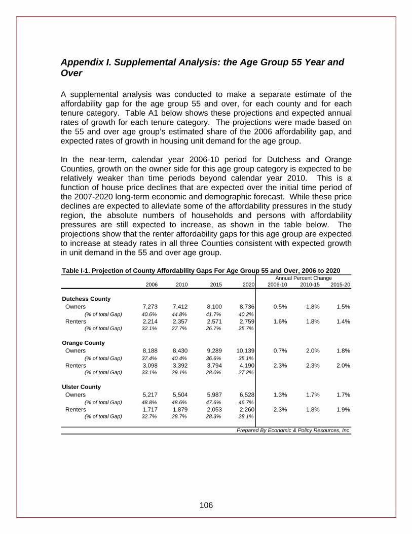
106

Appendix I. Supplemental Analysis: the Age Group 55 Year and Over A supplemental analysis was conducted to make a separate estimate of the affordability gap for the age group 55 and over, for each county and for each tenure category. Table A1 below shows these projections and expected annual rates of growth for each tenure category. The projections were made based on the 55 and over age group’s estimated share of the 2006 affordability gap, and expected rates of growth in housing unit demand for the age group. In the near-term, calendar year 2006-10 period for Dutchess and Orange Counties, growth on the owner side for this age group category is expected to be relatively weaker than time periods beyond calendar year 2010. This is a function of house price declines that are expected over the initial time period of the 2007-2020 long-term economic and demographic forecast. While these price declines are expected to alleviate some of the affordability pressures in the study region, the absolute numbers of households and persons with affordability pressures are still expected to increase, as shown in the table below. The projections show that the renter affordability gaps for this age group are expected to increase at steady rates in all three Counties consistent with expected growth in unit demand in the 55 and over age group. Table I-1. Projection of County Affordability Gaps For Age Group 55 and Over, 2006 to 2020

2006 2010 2015 2020 2006-10 2010-15 2015-20

Dutchess County Owners 7,273 7,412 8,100 8,736 0.5% 1.8% 1.5%

(% of total Gap) 40.6% 44.8% 41.7% 40.2% Renters 2,214 2,357 2,571 2,759 1.6% 1.8% 1.4%

(% of total Gap) 32.1% 27.7% 26.7% 25.7%

Orange County Owners 8,188 8,430 9,289 10,139 0.7% 2.0% 1.8%


(% of total Gap) 33.1% 29.1% 28.0% 27.2%

Ulster County Owners 5,217 5,504 5,987 6,528 1.3% 1.7% 1.7%


(% of total Gap) 32.7% 28.7% 28.3% 28.1%



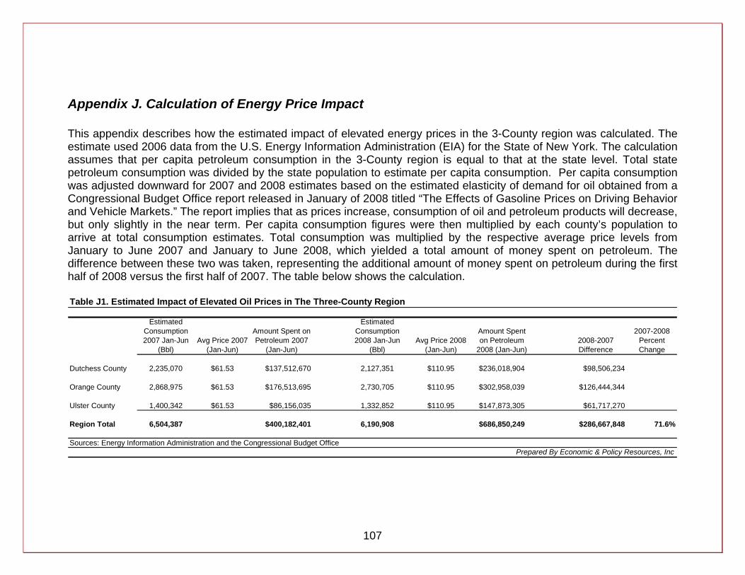
107

Appendix J. Calculation of Energy Price Impact This appendix describes how the estimated impact of elevated energy prices in the 3-County region was calculated. The estimate used 2006 data from the U.S. Energy Information Administration (EIA) for the State of New York. The calculation assumes that per capita petroleum consumption in the 3-County region is equal to that at the state level. Total state petroleum consumption was divided by the state population to estimate per capita consumption. Per capita consumption was adjusted downward for 2007 and 2008 estimates based on the estimated elasticity of demand for oil obtained from a Congressional Budget Office report released in January of 2008 titled “The Effects of Gasoline Prices on Driving Behavior and Vehicle Markets.” The report implies that as prices increase, consumption of oil and petroleum products will decrease, but only slightly in the near term. Per capita consumption figures were then multiplied by each county’s population to arrive at total consumption estimates. Total consumption was multiplied by the respective average price levels from January to June 2007 and January to June 2008, which yielded a total amount of money spent on petroleum. The difference between these two was taken, representing the additional amount of money spent on petroleum during the first half of 2008 versus the first half of 2007. The table below shows the calculation. Table J1. Estimated Impact of Elevated Oil Prices in The Three-County Region

Estimated Consumption 2007 Jan-Jun

(Bbl)Avg Price 2007

(Jan-Jun)

Amount Spent on Petroleum 2007

(Jan-Jun)

Estimated Consumption 2008 Jan-Jun

(Bbl)Avg Price 2008

(Jan-Jun)

Amount Spent on Petroleum

2008 (Jan-Jun)2008-2007 Difference

2007-2008 Percent Change

Dutchess County 2,235,070 $61.53 $137,512,670 2,127,351 $110.95 $236,018,904 $98,506,234

Orange County 2,868,975 $61.53 $176,513,695 2,730,705 $110.95 $302,958,039 $126,444,344

Ulster County 1,400,342 $61.53 $86,156,035 1,332,852 $110.95 $147,873,305 $61,717,270

Region Total 6,504,387 $400,182,401 6,190,908 $686,850,249 $286,667,848 71.6%

Sources: Energy Information Administration and the Congressional Budget OfficePrepared By Economic & Policy Resources, Inc

108

Appendix K. Glossary of Terms Affordability Gap: the difference between unit demand and unit supply, calculated by tenure and income category. Affordable House Price: the price of a house at which the amount paid toward housing costs does not exceed 30% of household income. This is consistent with the Department of Housing and Urban Development’s (HUD) definition of affordability, and for the purposes of this study takes into account costs associated with home ownership as described in the affordability calculations. Affordable Rent: the rent at which the amount paid toward housing costs does not exceed 30% of a household’s income. This is consistent with HUD’ definition of affordability, and takes into account the costs associated with renting as described in the affordability calculations. Bureau of Economic Analysis: the federal government agency charged with conducting analysis and maintaining economic data at the national, state and regional level. Bureau of Labor Statistics: a federal government agency that maintains a variety of economic and labor related data, such as wages, employment and unemployment, and inflation statistics. Consumer Price Index: a commonly used measure of inflation that is produced by the BLS. Cornell Institute for Social and Economic Research (CISER): a research department of Cornell University that maintains a variety of demographic and economic data, some of which was used in this study. Correlation: the tendency of two variables to move up and down together. Home Owners Insurance: insurance purchased by home owners to cover loss incurred by natural causes and by other events such as robbery or fire. House-Cost Burdened: a household spending 30% or more of household income on housing costs. Household: a household is defined as all members that live together in a housing unit, not including group quarters or institutions like colleges or prisons. Housing Unit: a physical structure

109

Housing Wage: the wage required to affordably purchase a median price home or a two bedroom apartment. Housing Wage Earnings Multiple: the number of earners needed in a household, earning a specific wage, for the household to be able to affordably purchase a median-priced home or two-bedroom apartment. For example, an earnings multiple of 2 indicates that 2 wage earners would be needed in order to avoid being house cost-burdened. Median Household Income: a central measure of household income. Median income in this study always refers to County median household income. Municipality: for the purpose of this study municipality refers to the towns and cities in the 3-County region. Private Mortgage Insurance: insurance required by most lenders that protects the lender against mortgage default. The borrower pays a monthly premium until 20% of the mortgage is paid off. The assumed rate in this study is 0.0078% per $1000 in mortgage value. Regression Analysis: a statistical analysis often employed by economists in order to determine the relationship between two or more variables. Seasonal Units: housing units that are occasionally occupied or for recreational use, as defined by the U.S. Census. Severely House-Cost Burdened: a household spending 50% or more of household income on housing costs. Study Region: the study region consists of Dutchess, Orange and Ulster Counties. Utility Costs: costs incurred by homeowners and renters for electricity, water and heating services. The BLS Consumer Expenditure Survey for 2003 to 2006 is used as a source in this study to estimate utility costs for home owners and renters. Vacancy Rate: the number of unoccupied housing units divided by the total number of housing units; a vacancy rate is calculated for both owner occupied units and renter occupied units. Weighted Average: a weighted average determines how much influence a factor has in the calculation of an average. The more weight assigned to a factor the more influence it has in the calculation. This is opposed to a simple average where each factor has equal weight in the outcome.

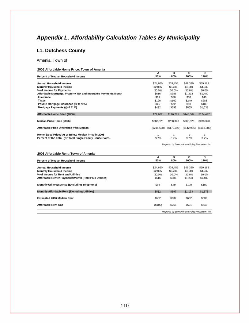
110

Appendix L. Affordability Calculation Tables By Municipality L1. Dutchess County Amenia, Town of 2006 Affordable Home Price: Town of Amenia


Annual Household Income $24,660 $39,456 $49,320 $59,183Monthly Household Income $2,055 $3,288 $4,110 $4,932% of Income for Payments 30.0% 30.0% 30.0% 30.0%Affordable Mortgage, Property Tax and Insurance Payments/Month $616 $986 $1,233 $1,480 Insurance $19 $30 $38 $46 Taxes $120 $192 $240 $288 Private Mortgage Insurance (@ 0.78%) $45 $72 $90 $108 Mortgage Payments (@ 6.41%) $432 $692 $865 $1,038






2006 Affordable Rent: Town of AmeniaA B C D

Percent of Median Household Income 50% 80% 100% 120%

Annual Household Income $24,660 $39,456 $49,320 $59,183Monthly Household Income $2,055 $3,288 $4,110 $4,932% of Income for Rent and Utilities 30.0% 30.0% 30.0% 30.0%Affordable Renter Payments/Month (Rent Plus Utilities) $616 $986 $1,233 $1,480






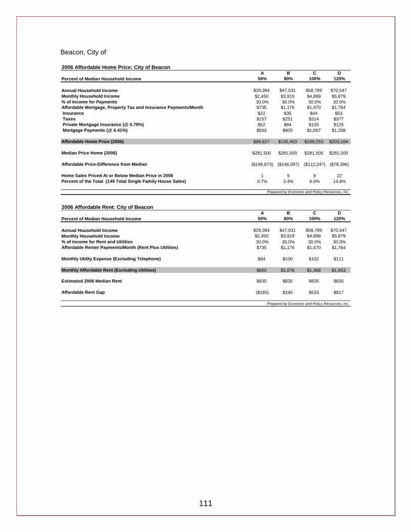
111

Beacon, City of 2006 Affordable Home Price: City of Beacon








2006 Affordable Rent: City of BeaconA B C D








112

Beekman, Town of 2006 Affordable Home Price: Town of Beekman


Annual Household Income $40,962 $65,539 $81,923 $98,308Monthly Household Income $3,413 $5,462 $6,827 $8,192% of Income for Payments 30.0% 30.0% 30.0% 30.0%Affordable Mortgage, Property Tax and Insurance Payments/Month $1,024 $1,638 $2,048 $2,458 Insurance $32 $51 $63 $76 Taxes $199 $319 $398 $478 Private Mortgage Insurance (@ 0.78%) $75 $119 $149 $179 Mortgage Payments (@ 6.41%) $719 $1,150 $1,437 $1,725






2006 Affordable Rent: Town of BeekmanA B C D


Annual Household Income $40,962 $65,539 $81,923 $98,308Monthly Household Income $3,413 $5,462 $6,827 $8,192% of Income for Rent and Utilities 30.0% 30.0% 30.0% 30.0%Affordable Renter Payments/Month (Rent Plus Utilities) $1,024 $1,638 $2,048 $2,458



Estimated 2006 Median Rent $1,015 $1,015 $1,015 $1,015



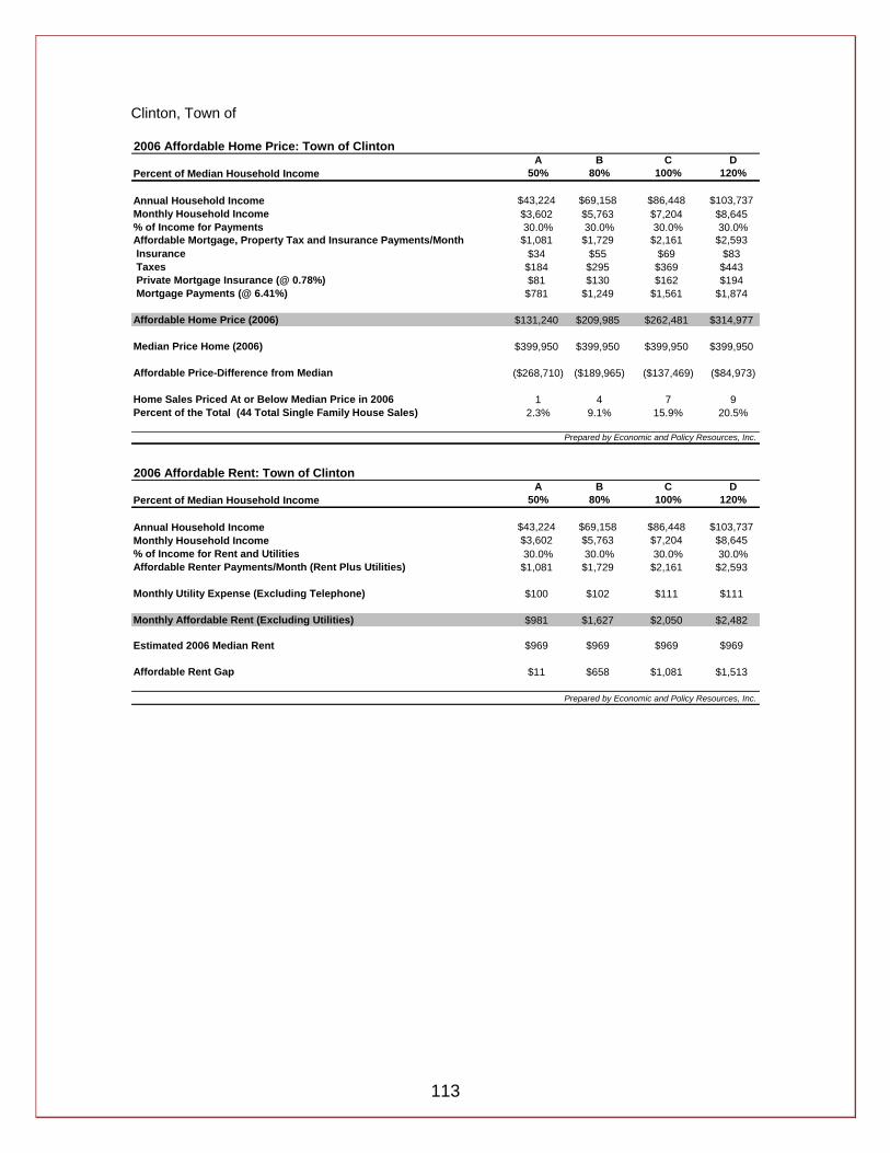
113

Clinton, Town of 2006 Affordable Home Price: Town of Clinton








2006 Affordable Rent: Town of ClintonA B C D






Affordable Rent Gap $11 $658 $1,081 $1,513


114

Dover, Town of 2006 Affordable Home Price: Town of Dover








2006 Affordable Rent: Town of DoverA B C D








115

East Fishkill, Town of 2006 Affordable Home Price: Town of East Fishkill








2006 Affordable Rent: Town of East FishkillA B C D




Monthly Affordable Rent (Excluding Utilities) $1,188 $1,953 $2,469 $2,985


Affordable Rent Gap $413 $1,178 $1,694 $2,210


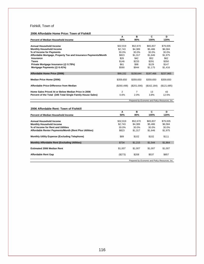
116

Fishkill, Town of 2006 Affordable Home Price: Town of Fishkill








2006 Affordable Rent: Town of FishkillA B C D








117

Hyde Park, Town of 2006 Affordable Home Price: Town of Hyde Park








2006 Affordable Rent: Town of Hyde ParkA B C D








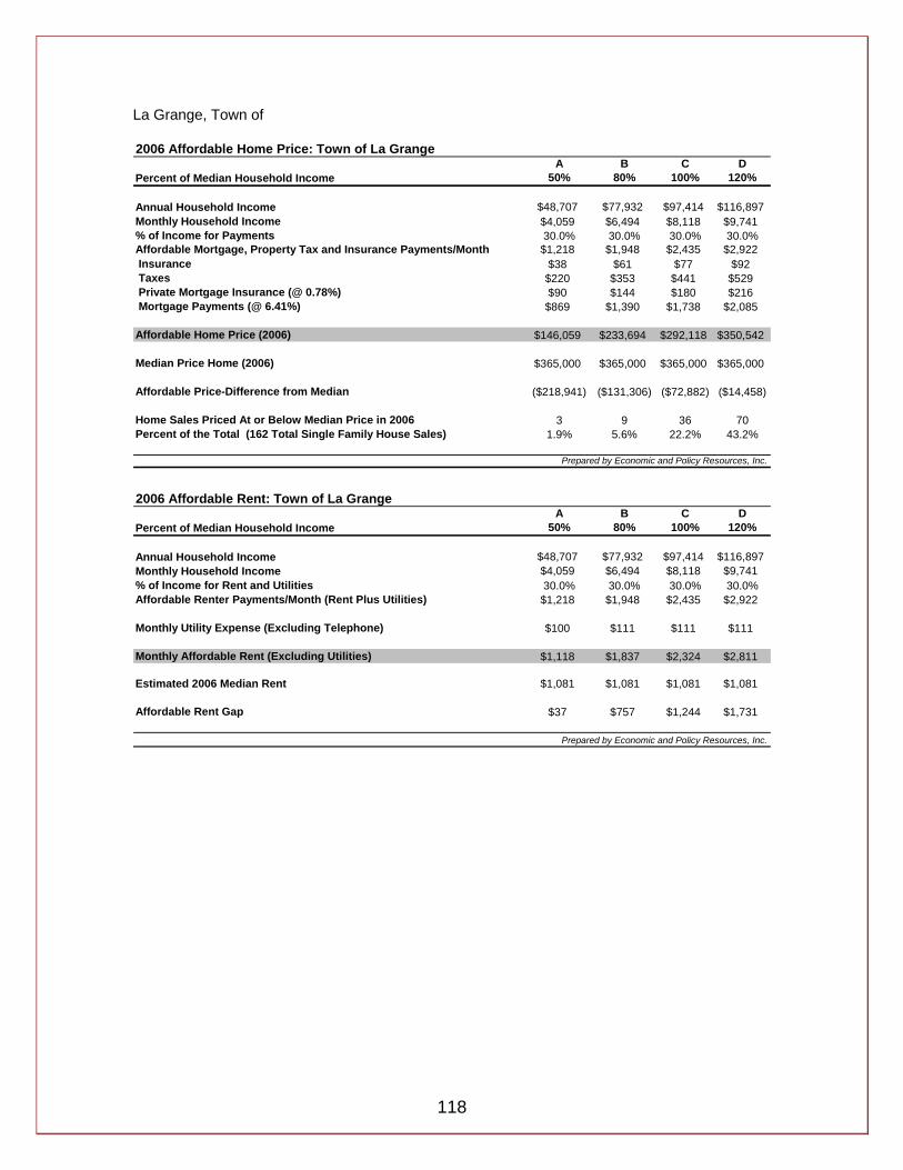
118

La Grange, Town of 2006 Affordable Home Price: Town of La Grange








2006 Affordable Rent: Town of La GrangeA B C D








119

Milan, Town of 2006 Affordable Home Price: Town of Milan


Annual Household Income $36,648 $58,636 $73,295 $87,954Monthly Household Income $3,054 $4,886 $6,108 $7,330% of Income for Payments 30.0% 30.0% 30.0% 30.0%Affordable Mortgage, Property Tax and Insurance Payments/Month $916 $1,466 $1,832 $2,199 Insurance $29 $47 $58 $70 Taxes $158 $252 $315 $378 Private Mortgage Insurance (@ 0.78%) $69 $110 $137 $165 Mortgage Payments (@ 6.41%) $661 $1,058 $1,322 $1,586






2006 Affordable Rent: Town of MilanA B C D






Affordable Rent Gap $79 $616 $973 $1,339


120

North East, Town of 2006 Affordable Home Price: Town of North East








2006 Affordable Rent: Town of North EastA B C D








121

Pawling, Town of 2006 Affordable Home Price: Town of Pawling








2006 Affordable Rent: Town of PawlingA B C D








122

Pine Plains, Town of 2006 Affordable Home Price: Town of Pine Plains








2006 Affordable Rent: Town of Pine PlainsA B C D








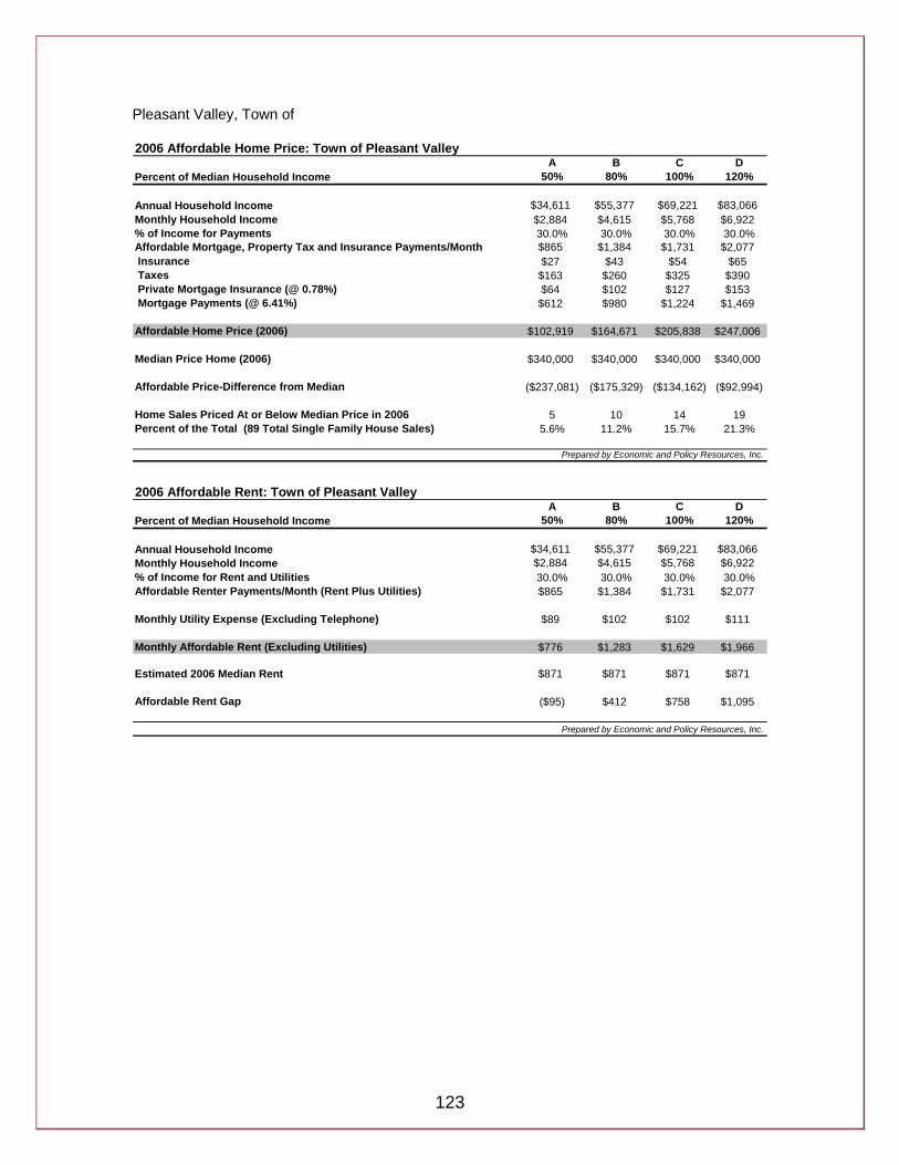
123

Pleasant Valley, Town of 2006 Affordable Home Price: Town of Pleasant Valley








2006 Affordable Rent: Town of Pleasant ValleyA B C D








124

Poughkeepsie, City of 2006 Affordable Home Price: City of Poughkeepsie


Annual Household Income $17,427 $27,883 $34,853 $41,824Monthly Household Income $1,452 $2,324 $2,904 $3,485% of Income for Payments 30.0% 30.0% 30.0% 30.0%Affordable Mortgage, Property Tax and Insurance Payments/Month $436 $697 $871 $1,046 Insurance $13 $20 $25 $31 Taxes $104 $166 $208 $250 Private Mortgage Insurance (@ 0.78%) $30 $48 $60 $72 Mortgage Payments (@ 6.41%) $289 $462 $578 $693






2006 Affordable Rent: City of PoughkeepsieA B C D


Annual Household Income $17,427 $27,883 $34,853 $41,824Monthly Household Income $1,452 $2,324 $2,904 $3,485% of Income for Rent and Utilities 30.0% 30.0% 30.0% 30.0%Affordable Renter Payments/Month (Rent Plus Utilities) $436 $697 $871 $1,046


Monthly Affordable Rent (Excluding Utilities) $355 $613 $782 $946


Affordable Rent Gap ($373) ($115) $54 $218


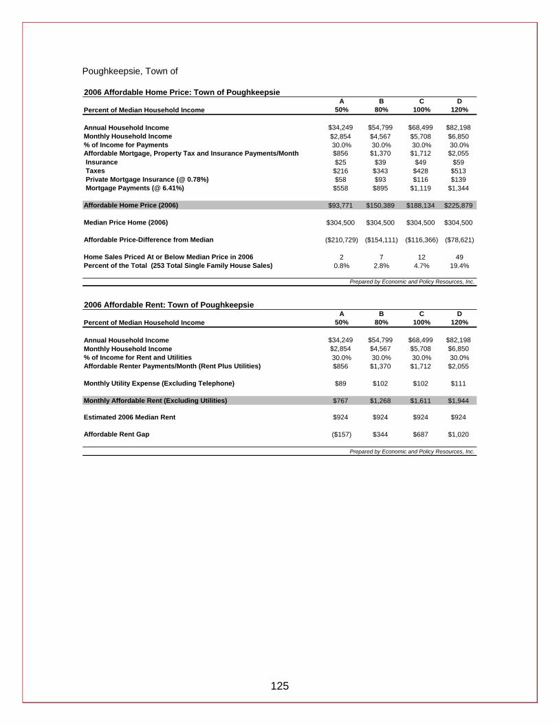
125

Poughkeepsie, Town of 2006 Affordable Home Price: Town of Poughkeepsie








2006 Affordable Rent: Town of PoughkeepsieA B C D








126

Red Hook, Town of 2006 Affordable Home Price: Town of Red Hook








2006 Affordable Rent: Town of Red HookA B C D








127

Rhinebeck, Town of 2006 Affordable Home Price: Town of Rhinebeck








2006 Affordable Rent: Town of RhinebeckA B C D








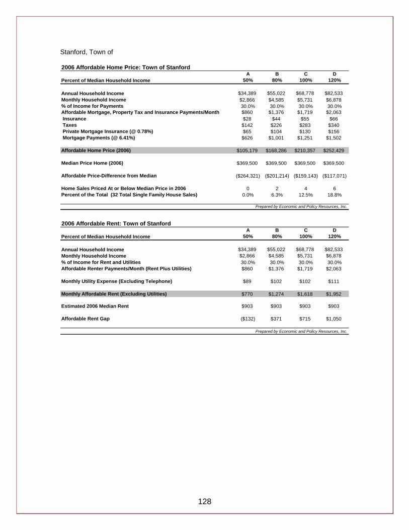
128

Stanford, Town of 2006 Affordable Home Price: Town of Stanford








2006 Affordable Rent: Town of StanfordA B C D








129

Union Vale, Town of 2006 Affordable Home Price: Town of Union Vale








2006 Affordable Rent: Town of Union ValeA B C D








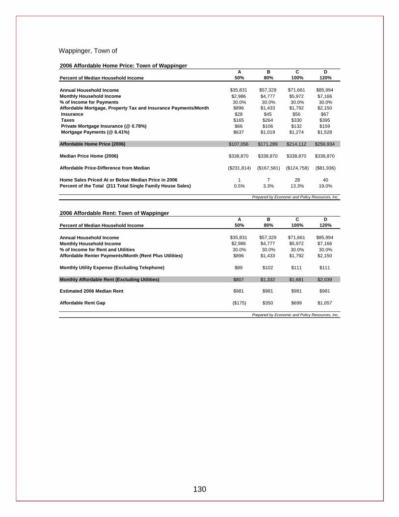
130

Wappinger, Town of 2006 Affordable Home Price: Town of Wappinger








2006 Affordable Rent: Town of WappingerA B C D








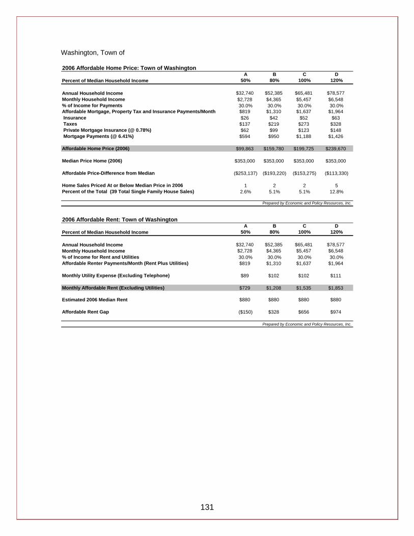
131

Washington, Town of 2006 Affordable Home Price: Town of Washington








2006 Affordable Rent: Town of WashingtonA B C D








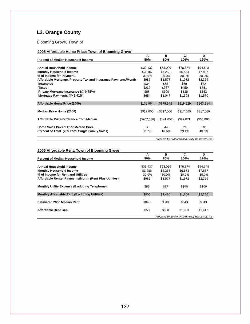
132

L2. Orange County Blooming Grove, Town of 2006 Affordable Home Price: Town of Blooming Grove






Home Sales Priced At or Median Price 7 44 78 106Percent of Total (265 Total Single Family Sales) 2.6% 16.6% 29.4% 40.0%


2006 Affordable Rent: Town of Blooming GroveA B C D








133

Chester, Town of 2006 Affordable Home Price: Town of Chester








2006 Affordable Rent: Town of ChesterA B C D






Affordable Rent Gap ($10) $613 $1,021 $1,438


134

Cornwall, Town of 2006 Affordable Home Price: Town of Cornwall








2006 Affordable Rent: Town of CornwallA B C D








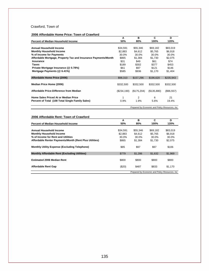
135

Crawford, Town of 2006 Affordable Home Price: Town of Crawford








2006 Affordable Rent: Town of CrawfordA B C D








136

Deerpark, Town of 2006 Affordable Home Price: Town of Deerpark








2006 Affordable Rent: Town of DeerparkA B C D








137

Goshen, Town of 2006 Affordable Home Price: Town of Goshen








2006 Affordable Rent: Town of GoshenA B C D








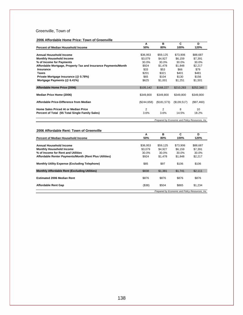
138

Greenville, Town of 2006 Affordable Home Price: Town of Greenville








2006 Affordable Rent: Town of GreenvilleA B C D








139

Hamptonburgh, Town of 2006 Affordable Home Price: Town of Highlands








2006 Affordable Rent: Town of HighlandsA B C D








140

Highlands, Town of 2006 Affordable Home Price: Town of Highlands








2006 Affordable Rent: Town of HighlandsA B C D








141

Middletown, City of 2006 Affordable Home Price: City of Middletown


Annual Household Income $23,650 $37,841 $47,301 $56,761Monthly Household Income $1,971 $3,153 $3,942 $4,730% of Income for Payments 30.0% 30.0% 30.0% 30.0%Affordable Mortgage, Property Tax and Insurance Payments/Month $591 $946 $1,183 $1,419 Insurance $20 $32 $40 $48 Taxes $152 $244 $304 $365 Private Mortgage Insurance (@ 0.78%) $39 $63 $79 $95 Mortgage Payments (@ 6.41%) $380 $607 $759 $911






2006 Affordable Rent: City of MiddletownA B C D








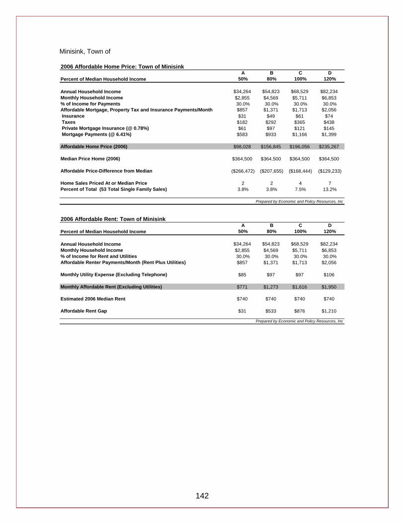
142

Minisink, Town of 2006 Affordable Home Price: Town of Minisink








2006 Affordable Rent: Town of MinisinkA B C D








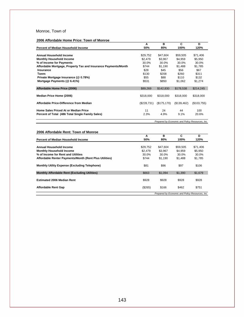
143

Monroe, Town of 2006 Affordable Home Price: Town of Monroe








2006 Affordable Rent: Town of MonroeA B C D








144

Montgomery, Town of 2006 Affordable Home Price: Town of Montgomery








2006 Affordable Rent: Town of MontgomeryA B C D








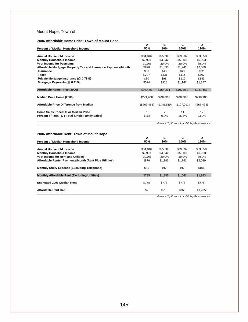
145

Mount Hope, Town of 2006 Affordable Home Price: Town of Mount Hope








2006 Affordable Rent: Town of Mount HopeA B C D








146

New Windsor, Town of 2006 Affordable Home Price: Town of New Windsor








2006 Affordable Rent: Town of New WindsorA B C D








147

Newburgh, City of 2006 Affordable Home Price: City of Newburgh








2006 Affordable Rent: City of NewburghA B C D




Monthly Affordable Rent (Excluding Utilities) $380 $651 $829 $1,002




148

Newburgh, Town of 2006 Affordable Home Price: Town of Newburgh








2006 Affordable Rent: Town of NewburghA B C D








149

Port Jervis, City of 2006 Affordable Home Price: City of Port Jervis








2006 Affordable Rent: City of Port JervisA B C D




Monthly Affordable Rent (Excluding Utilities) $368 $631 $805 $973



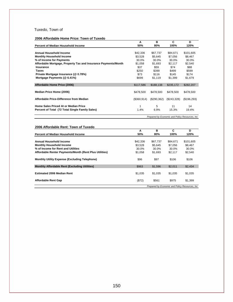
150

Tuxedo, Town of 2006 Affordable Home Price: Town of Tuxedo








2006 Affordable Rent: Town of TuxedoA B C D








151

Wallkill, Town of 2006 Affordable Home Price: Town of Wallkill








2006 Affordable Rent: Town of WallkillA B C D








152

Warwick, Town of 2006 Affordable Home Price: Town of Warwick








2006 Affordable Rent: Town of WarwickA B C D








153

Wawayanda, Town of 2006 Affordable Home Price: Town of Wawayanda








2006 Affordable Rent: Town of WawayandaA B C D








154

Woodbury, Town of 2006 Affordable Home Price: Town of Woodbury








2006 Affordable Rent: Town of WoodburyA B C D








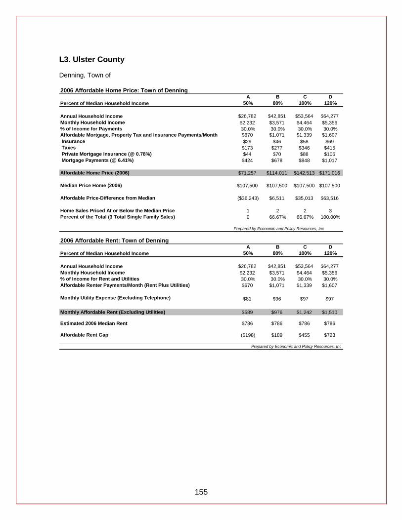
155

L3. Ulster County Denning, Town of 2006 Affordable Home Price: Town of Denning





Affordable Price-Difference from Median ($36,243) $6,511 $35,013 $63,516

Home Sales Priced At or Below the Median Price 1 2 2 3Percent of the Total (3 Total Single Family Sales) 0 66.67% 66.67% 100.00%


2006 Affordable Rent: Town of DenningA B C D








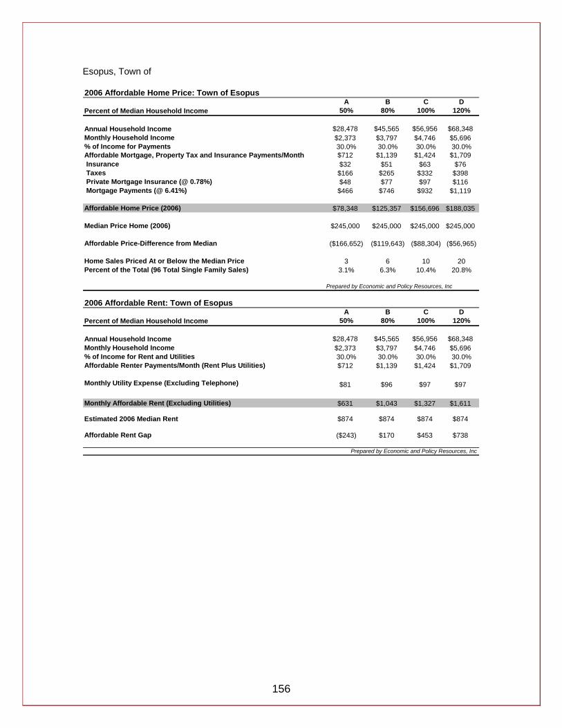
156

Esopus, Town of 2006 Affordable Home Price: Town of Esopus








2006 Affordable Rent: Town of EsopusA B C D








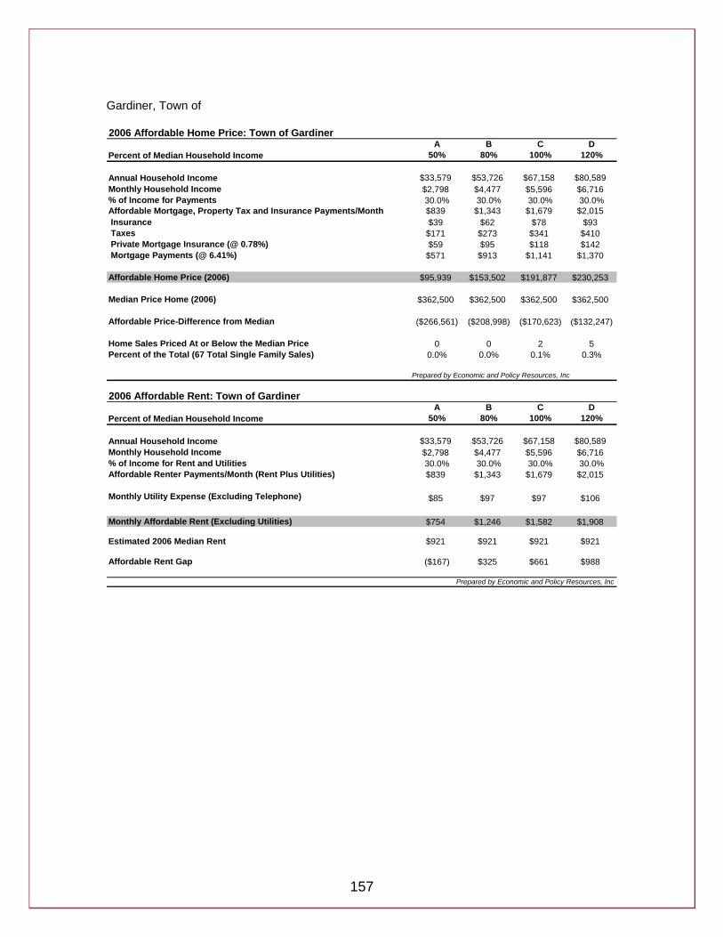
157

Gardiner, Town of 2006 Affordable Home Price: Town of Gardiner








2006 Affordable Rent: Town of GardinerA B C D








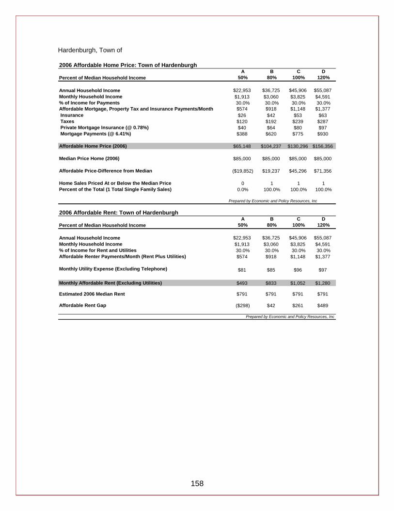
158

Hardenburgh, Town of 2006 Affordable Home Price: Town of Hardenburgh





Affordable Price-Difference from Median ($19,852) $19,237 $45,296 $71,356



2006 Affordable Rent: Town of HardenburghA B C D








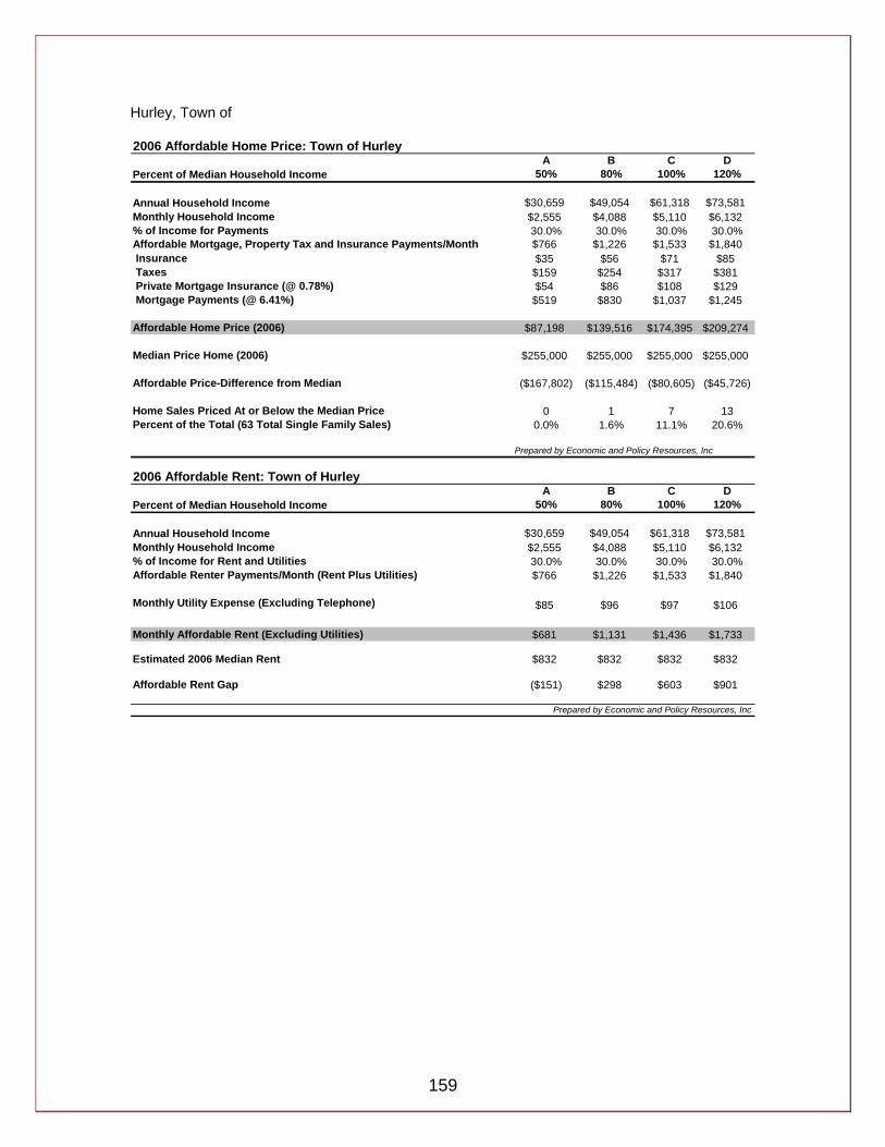
159

Hurley, Town of 2006 Affordable Home Price: Town of Hurley








2006 Affordable Rent: Town of HurleyA B C D








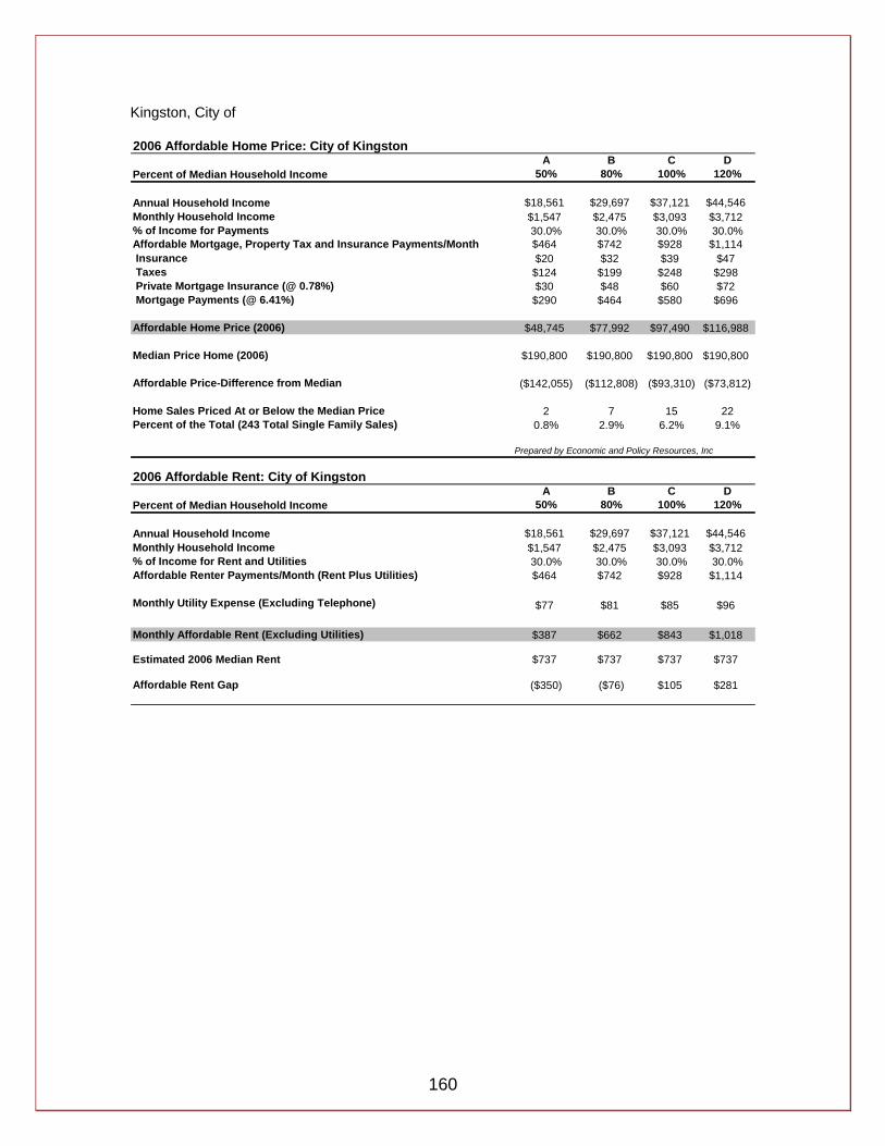
160

Kingston, City of 2006 Affordable Home Price: City of Kingston








2006 Affordable Rent: City of KingstonA B C D







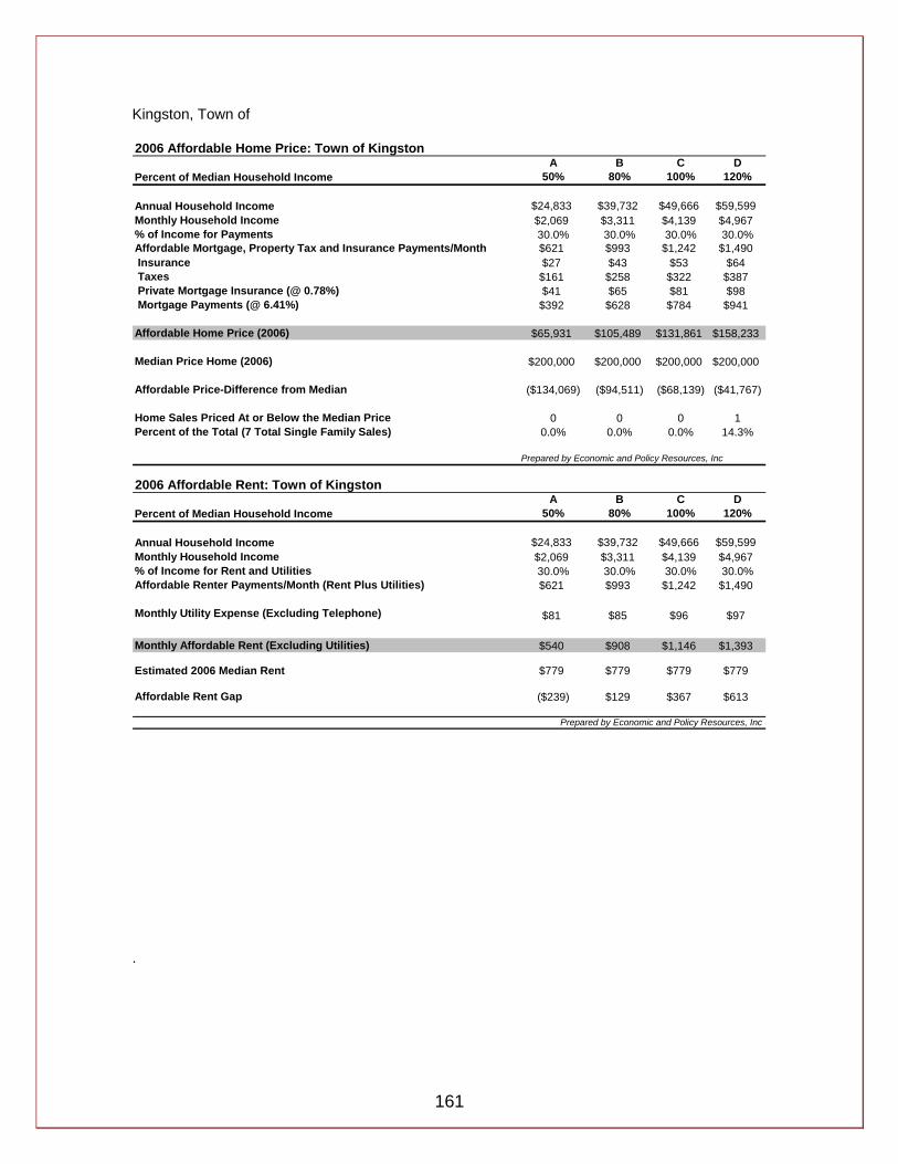
161

Kingston, Town of 2006 Affordable Home Price: Town of Kingston








2006 Affordable Rent: Town of KingstonA B C D







Prepared by Economic and Policy Resources, Inc .

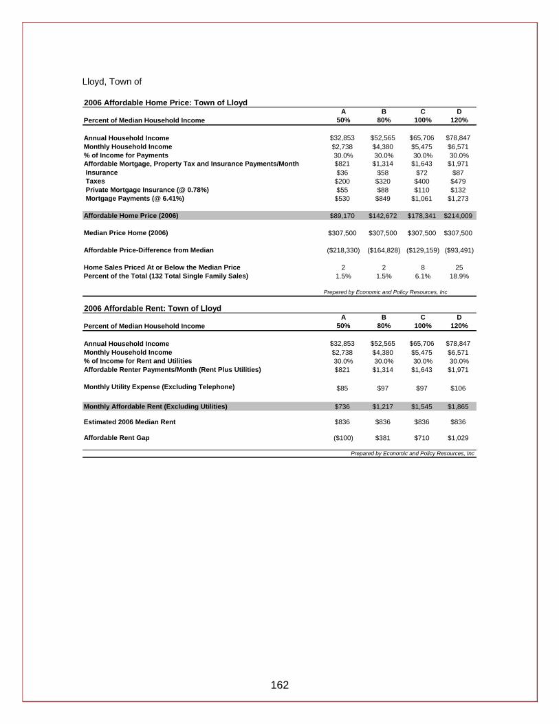
162

Lloyd, Town of 2006 Affordable Home Price: Town of Lloyd








2006 Affordable Rent: Town of LloydA B C D








163

Marbletown, Town of 2006 Affordable Home Price: Town of Marbletown








2006 Affordable Rent: Town of MarbletownA B C D








164

Marlborough, Town of 2006 Affordable Home Price: Town of Marlborough








2006 Affordable Rent: Town of MarlboroughA B C D








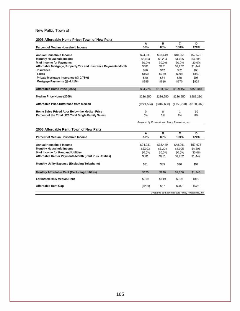
165

New Paltz, Town of 2006 Affordable Home Price: Town of New Paltz






Home Sales Priced At or Below the Median Price 0 0 1 10Percent of the Total (126 Total Single Family Sales) 0% 0% 1% 8%


2006 Affordable Rent: Town of New PaltzA B C D








166

Olive, Town of 2006 Affordable Home Price: Town of Olive








2006 Affordable Rent: Town of OliveA B C D








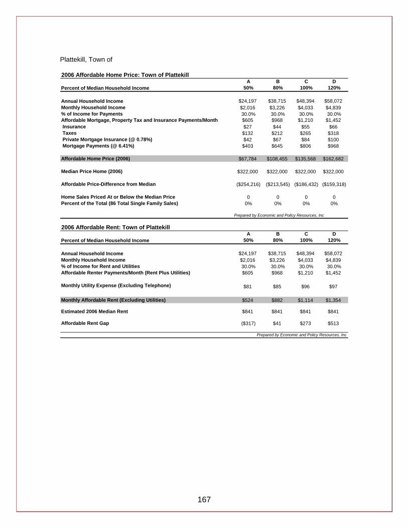
167

Plattekill, Town of 2006 Affordable Home Price: Town of Plattekill






Home Sales Priced At or Below the Median Price 0 0 0 0Percent of the Total (86 Total Single Family Sales) 0% 0% 0% 0%


2006 Affordable Rent: Town of PlattekillA B C D








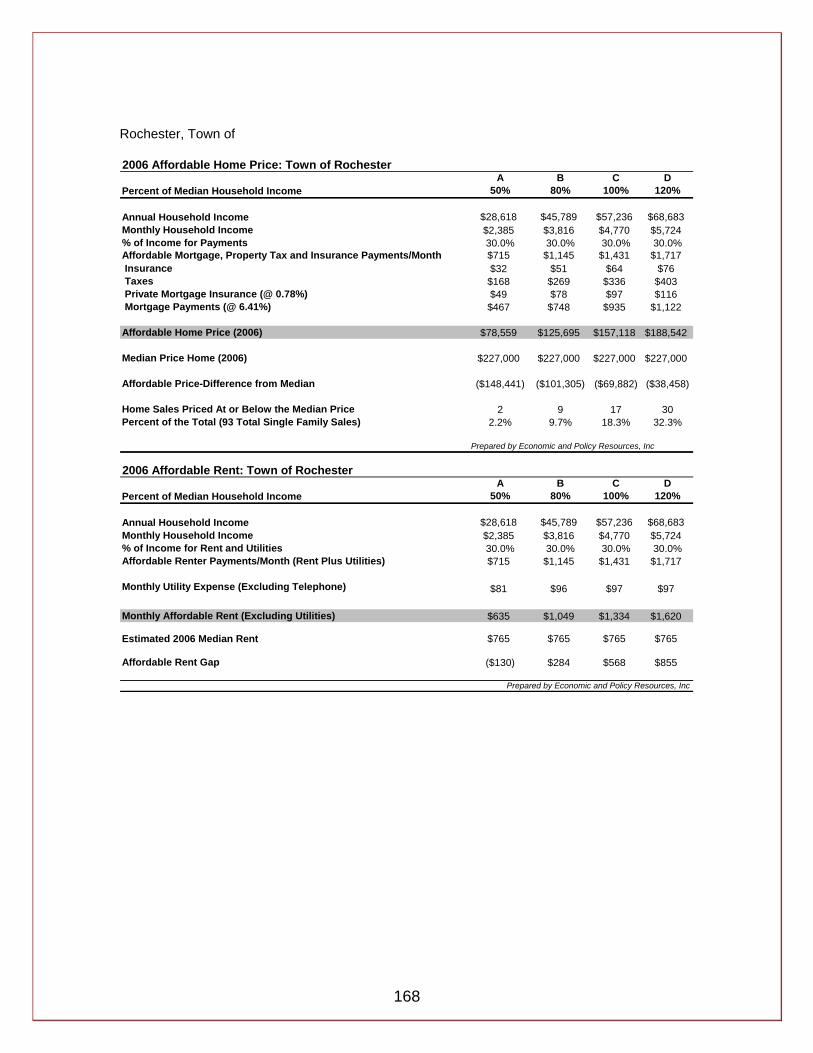
168

Rochester, Town of 2006 Affordable Home Price: Town of Rochester








2006 Affordable Rent: Town of RochesterA B C D








169

Rosendale, Town of 2006 Affordable Home Price: Town of Rosendale








2006 Affordable Rent: Town of RosendaleA B C D








170

Saugerties, Town of 2006 Affordable Home Price: Town of Saugerties








2006 Affordable Rent: Town of SaugertiesA B C D








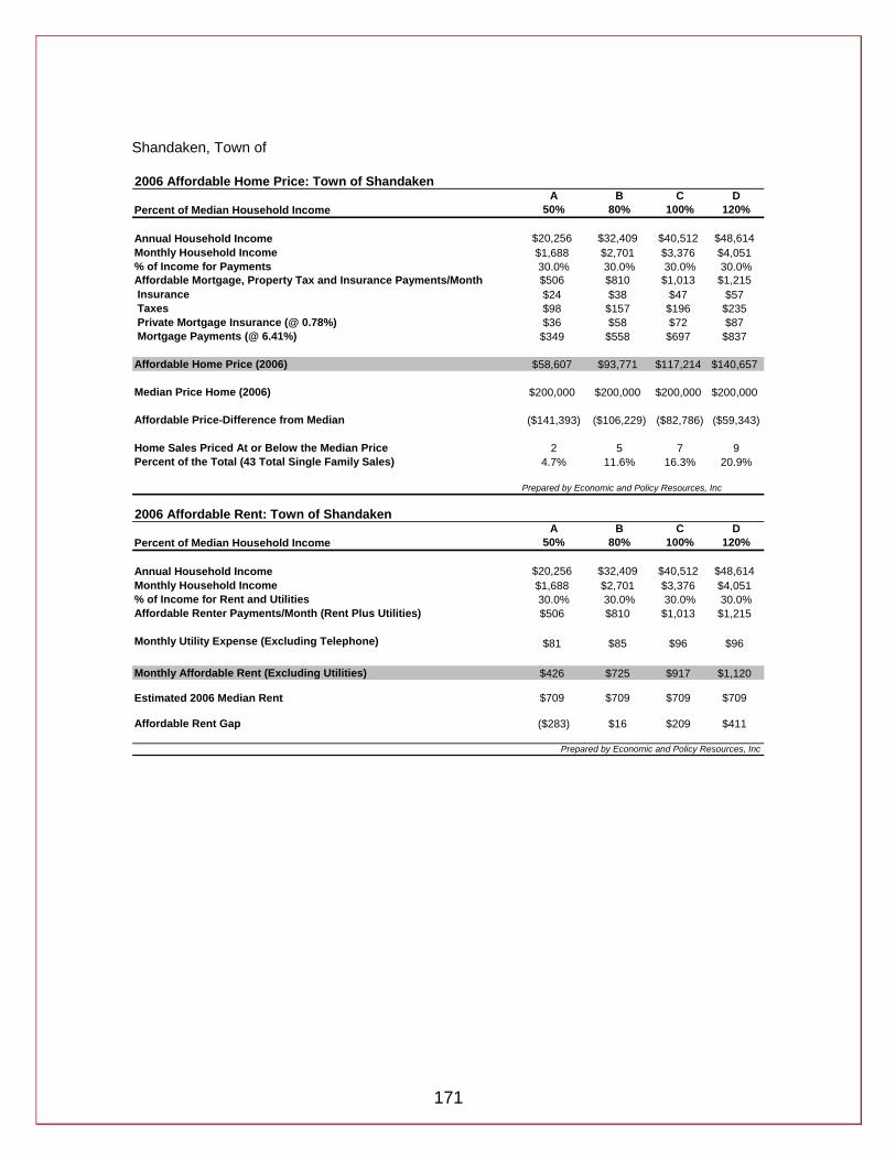
171

Shandaken, Town of 2006 Affordable Home Price: Town of Shandaken








2006 Affordable Rent: Town of ShandakenA B C D








172

Shawangunk, Town of 2006 Affordable Home Price: Town of Shawangunk








2006 Affordable Rent: Town of ShawangunkA B C D








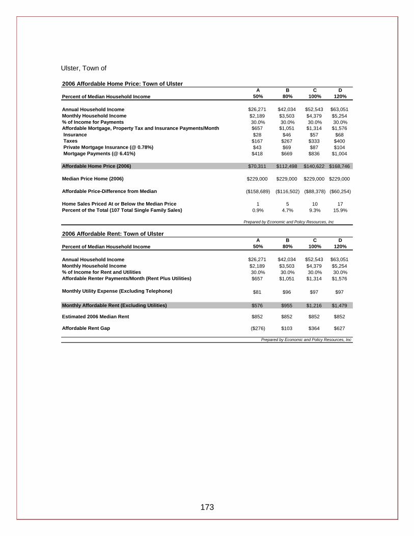
173

Ulster, Town of 2006 Affordable Home Price: Town of Ulster








2006 Affordable Rent: Town of UlsterA B C D








174

Wawarsing, Town of 2006 Affordable Home Price: Town of Wawarsing








2006 Affordable Rent: Town of WawarsingA B C D








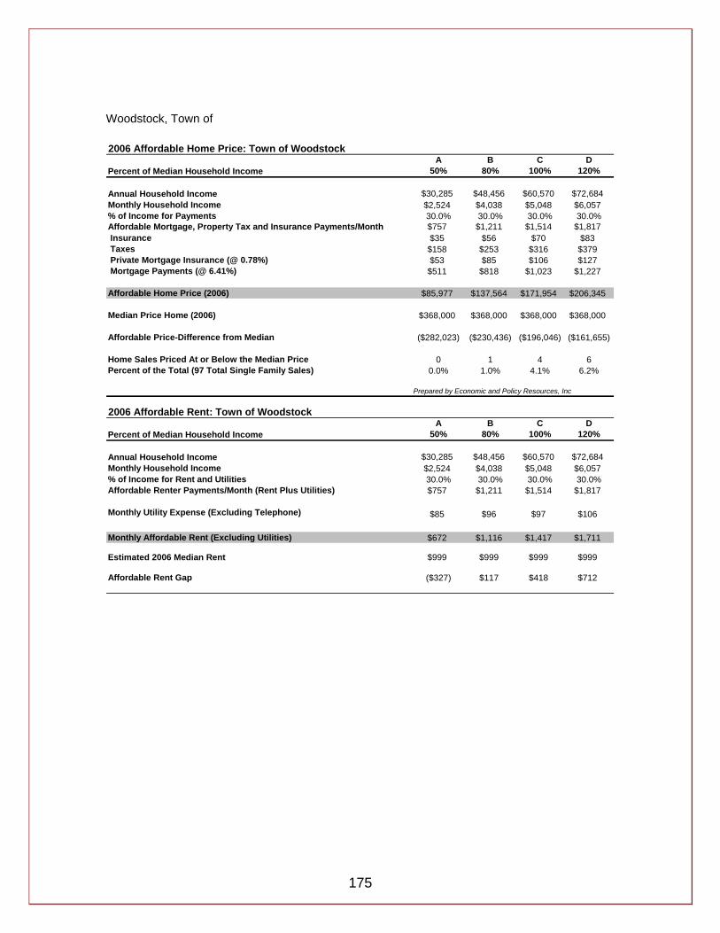
175

Woodstock, Town of 2006 Affordable Home Price: Town of Woodstock








2006 Affordable Rent: Town of WoodstockA B C D







A Three-County Regional Housing Needs Assessment:

Documents

Transcript of A Three-County Regional Housing Needs Assessment: