A theory of spatial structure in ecological communities at multiple spatial scales

179

Ecological Monographs, 75(2), 2005, pp. 179–197q 2005 by the Ecological Society of America

A THEORY OF SPATIAL STRUCTURE IN ECOLOGICAL COMMUNITIES ATMULTIPLE SPATIAL SCALES

JOHN HARTE,1,3 ERIN CONLISK,1 ANNETTE OSTLING,1 JESSICA L. GREEN,2 AND ADAM B. SMITH1

1Energy and Resources Group, University of California, Berkeley, California 94720 USA2School of Natural Sciences, University of California, Merced, California 95344 USA

Abstract. A theory of spatial structure in ecological communities is presented andtested. At the core of the theory is a simple allocation rule for the assembly of species inspace. The theory leads, with no adjustable parameters, to nonrandom statistical predictionsfor the spatial distribution of species at multiple spatial scales. The distributions are suchthat the abundance of a species at the largest measured scale uniquely determines the spatial-abundance distribution of the individuals of that species at smaller spatial scales. The shapeof the species–area relationship, the endemics–area relationship, a scale-dependent com-munity-level spatial-abundance distribution, the species-abundance distribution at smallspatial scales, an index of intraspecific aggregation, the range–area relationship, and thedependence of species turnover on interpatch distance and on patch size are also uniquelypredicted as a function solely of the list of abundances of the species at the largest spatialscale. We show that the spatial structure of three spatially explicit vegetation census datasets (i.e., a 64-m2 serpentine grassland plot, a 50-ha moist tropical forest plot, and a 9.68-ha dry tropical forest plot) are generally consistent with the predictions of the theory,despite the very simple statistical assumption upon which the theory is based, and theabsence of adjustable parameters. However, deviations between predicted and observeddistributions do arise for the species with the highest abundances; the pattern of thosedeviations indicates that the theory, which currently contains no explicit description ofinteraction mechanisms among individuals within species, could be improved with theincorporation of intraspecific density dependence.

Key words: abundance distribution; Barro Colorado Island (BCI), Panama; endemics–area re-lationship; range–area relationship; San Emilio, Costa Rica; scale dependence; serpentine grassland;spatial distribution; species–area relationship; tropical forest.

INTRODUCTION

Understanding the abundance and spatial distribu-tion of species at multiple spatial scales is a centralconcern of ecology (Fisher et al. 1943, Preston 1948,Krebs 1994, Rosenzweig 1995, Gaston and Blackburn2000, He and Legendre 2002). Patterns in the distri-butions of individuals and species across space provideinformation critical to our ability to decipher the forcesthat structure and maintain ecological diversity (Pielou1969, Brown et al. 1995). Within biomes, knowledgeof the scale-dependent frequency of patch occupancycan lead to improved estimates of extinction rates underperturbations, more effective land protection policies,the design of more efficient and accurate censusingstrategies, and improved estimates of species richnessfrom sparse census data (Whitmore and Sayer 1992,May et al. 1995, Rosenzweig 1995).

Spatial models that explicitly assume knowledge ofprocesses such as birth, death, dispersal, speciation,migration, extinction, and niche differentiation have

Manuscript received 7 September 2004; revised 3 November2004; accepted 4 November 2004. Corresponding Editor: W. S.C. Gurney.

3 E-mail: [email protected]

significantly advanced our understanding of patterns inthe abundance and distribution of species across spaceand time (see reviews by Hubbell [2001], Chave[2004], and Leibold et al. [2004]). Statistically basedmodels, while not derived from explicit biologicalmechanisms, also have provided a tractable theoreticalframework for quantifying the spatial structure of eco-logical communities. For example, in an early inves-tigation of the distribution and abundance of species,Preston (1962) and May (1975) argued that a particularspecies-abundance distribution (SAD), the canonicallognormal, was related to a power-law form of thespecies–area relationship (SAR). Their approach wasbased on randomly sampling individuals from an eco-logical community with a lognormal SAD. Coleman(1981) extended the reach of the random model,developing a general framework for deriving the shapeof the species–area relationship under arbitraryspecies-abundance distributions, while Green andOstling (2003) derived the form of an endemics–arearelationship under the random model. Although therandom distribution assumption does provide a generalmodel of spatial pattern in ecology, numerous studieshave shown that this assumption inadequately describesspatial patterns of aggregation of individuals within

180 JOHN HARTE ET AL. Ecological MonographsVol. 75, No. 2

species and of species across landscapes (Condit et al.1996b, 2002, Plotkin et al. 2000, Green et al. 2003).

To model aggregated species distributions, and toinvestigate the effect of aggregation on macroecolog-ical properties such as the SAR or species turnover, anumber of authors (Wright 1991, He and Gaston 2000,2003) have examined the following statistical model:

2k 2 2p 5 1 2 [(k 1 m)/k] k 5 m /(s 2 m) (1)

where p is the probability of a species occurrence in agrid cell as a function of the mean occupancy m, thevariance s2, and a parameter k, that can take on valuesk , 2m or k . 0 and that can be estimated from censusdata (Bliss and Fisher 1953). In general, k will be spe-cies and scale dependent (Plotkin and Muller-Landau2002). For positive k values, the model derives fromthe negative binomial distribution (NBD), which hasbeen used in the following ways: to describe SARs andabundance–aggregation patterns (He and Gaston 2000,2003, He and Hubbell 2003), to derive a formula forthe fraction of species in common to two separated cellsof a specified area (Plotkin and Muller-Landau 2002),and to derive an ‘‘endemics–area relationship’’ (EAR)between the number of species in a cell that are uniqueto that cell and the area of the cell (Green and Ostling2003). In applications of the NBD, values of the pa-rameter k at every scale and for every species are de-termined from data, rather than from first principles,and thus the model contains a sizeable number of ad-justable parameters when applied to a community ofspecies. Plotkin et al. (2000) assumed and exploredanother spatial model based on the Poisson cluster dis-tribution; with even more adjustable parameters thanthe NBD, this model can generate a wide variety ofpatterns that resemble those observed in nature.

Another statistically based approach to describingspecies-level and community-level spatial patternsacross spatial scales has focused on the explicit scalingproperties of the SAR and, for individual species, therange–area relationship (RAR). The RAR describes thedependence of the range size of a species (defined bya box-counting procedure as the total area of all oc-cupied grid cells at a given scale) on cell area (Kunin1998, Gaston and Blackburn 2000, Harte et al. 2001).The scaling approach starts with the observation thatthe shape of the SAR and the RAR can be expressedin terms of certain fundamental probability parameters.At the species level, these probabilities describe howthe number of occupied census cells depends on thespatial scale of the cells (Harte et al. 2001), while atcommunity level, the probabilities describe how spe-cies richness depends on spatial scale (Harte et al. 1999,2001). The assumption of self-similarity, or fractality,is equivalent to the assumption that the probability pa-rameters are independent of scale (Ostling et al. 2003).When the community-level probabilities are scale in-dependent, a power-law SAR results; when the param-

eters for a particular species are scale independent, apower-law RAR results for that species. Although thetheory presented here is substantially different fromthis previous work, and we make no a priori assump-tions about the scaling properties of these probabilityparameters, it is convenient to express the theory withthose same parameters, and so formal definitions aregiven (see Theoretical background; The probability pa-rameters).

The statistical theory presented here departs in vary-ing ways from previous approaches. In one respect, ourapproach is similar to that of random placement modelsin that all the macroecological predictions follow froma single statistical assumption, along with knowledgeof the total abundances of the species (Coleman 1981).In particular, our results derive from what we denoteas the ‘‘hypothesis of equal allocation probabilities’’(HEAP). This fundamental statistical assumption isakin to, but significantly different in detail from, the‘‘hypothesis of equal a priori probabilities’’ that un-derpins statistical mechanics (Ruhla 1992). The latter,for classical molecules, results in a binomial abundancedistribution across space, as does the random placementmodel in ecology. Instead, HEAP results in a nonran-dom, more aggregated distribution of individuals.

In contrast to models based on the negative binomialor the Poisson cluster model, which contain adjustableparameters for each species, we introduce no adjustableparameters nor, in contrast to McGill and Collins(2003), do we require as input to our theory any em-pirical information about the shape of species-abun-dance distributions across the ranges of the species.However, our work shares with those approaches theobjective of rigorously deriving testable predictions forthe relationships among different macroecological pat-terns, such as the relationship between species-levelaggregation or RAR curves and community propertiessuch as the SAR or species turnover in space.

In contrast to our previous work on fractal scalingproperties of species distributions, we impose here atop-down boundary condition on the recursion relationsthat generate the probability distribution for each spe-cies; the boundary condition at the ‘‘top’’ is simply thetotal abundance of a species in some large area. Where-as the bottom-up approach requires prior knowledge ofthe species-level probability parameters describing theRAR at all spatial scales being considered, our top-down approach uniquely predicts the values of all thoseparameters, along with the community-level probabil-ity parameters describing the SAR at all scales as afunction solely of the list of total abundances of thespecies (the SAD) within the large area.

Assuming a SAD at some largest scale, our theorypredicts scale-dependent probability distributions de-scribing a wide range of ecological patterns at bothspecies and community levels at multiple spatial scales.For each species, it predicts the distribution of patchoccupancy frequencies across multiple spatial scales,

May 2005 181SPATIAL-ABUNDANCE DISTRIBUTION

the RAR, an ‘‘O-ring’’ index of spatial clustering (Con-dit et al. 2000), and the scaling behavior of the mean–variance relationship for the species-level spatial dis-tributions. At community level, it predicts the scale-dependent patch occupancy distribution for total abun-dances summed over all species, as well as the SAR,the EAR, the SAD at all smaller spatial scales, andspecies turnover as a function of census patch area andinterpatch distance. Knowledge of the SAD at somelargest spatial scale is all that is needed by the theoryto uniquely generate all these spatial properties of eco-systems at smaller scales.

Although power-law SARs are not assumed here, andin fact under HEAP can never hold over all scales,HEAP can predict the SADs for which a power-lawSAR will arise over a limited scale range. On the otherhand, the theory predicts that the species-level prob-ability parameters can never be scale independent, andthus the RARs cannot have exact power-law behavior,over any scale range. More specifically, it predicts thaton log–log plots, the RAR for each species will alwaysexhibit negative curvature, the strength of which at anyscale depends on the abundance of the species.

Our approach here is to create a theory of spatialstructure in macroecology that can be tested against awide array of empirical spatial patterns in ecosystems.Because the theory contains no adjustable parametersand no explicit biological mechanisms such as densitydependence, dispersal, birth, death, and interspecificinteractions, we expect the theory to perform poorlyunder at least some circumstances. From knowledge ofthe patterns of success and failure when we comparethe theoretical predictions with data from three sitesfor which spatially explicit plant census data are avail-able, we show that we can gain insight into which ofthe many neglected biological mechanisms are likelyto most significantly influence spatial patterns in ecol-ogy. Because our fundamental statistical assumptionleads to predictions that greatly outperform randomplacement predictions, we argue that HEAP is a useful‘‘null assumption’’ for macroecology. Although wecurrently lack a mechanistic understanding of the originof HEAP, we suggest that an alternative formulation ofthe theory in terms of a spatially explicit ‘‘assemblyfunction’’ may provide the basis for such an under-standing.

THEORETICAL BACKGROUND

Types of abundance distributions

Consider a plot or landscape of area A0 populated byS0 species, each containing a total of individuals,( j )n0

where ( j ) is a species label that ranges from j 5 1 . . .S0. To introduce a scale parameter, let A0 be repeatedlybisected into similar-shaped patches. Then we can de-fine a scale parameter i such that patches of area Ai areformed from the ith bisection (Harte et al. 1999). Notethat larger spatial scales correspond to smaller values

of i. A formal procedure for this bisection process ex-ists (Harte et al. 1999, Plotkin et al. 2000, Ostling etal. 2003) and a consistent procedure for avoiding po-tentially unrealistic, artifactual consequences has beendescribed (Ostling et al. 2004).

We distinguish here two related types of, potentiallyscale-dependent abundance distributions: the species-abundance distribution and spatial-abundance distri-butions. We denote the former by Fi(n); it is the dis-tribution of abundances across all the species in a com-munity at scale i. The meaning of Fi(n) is based on theidea of a species occurrence or nonoccurrence at scalei. At scale i 5 0, all S0 species occur and F0(n) is thecustomarily defined species-abundance distribution(Fisher et al. 1943, Preston 1948, Gaston and Black-burn 2000): the fraction of all the S0 species in A0 withn individuals. At finer scales, Fi(n) is a straightforwardgeneralization of this. For example, consider the twoA1 cells formed by the first bisection. There are 2S0

species occurrences or nonoccurrences in those twocells. Suppose there are f3 occurrences in which a spe-cies has 3 individuals in either one of the A1 cells; thenF1(3) 5 f3/(2S0). Note that F1(0) will be the fractionof nonoccurrences in the Ai cells and is thus nonzeroif at least one of the species is absent from one of thetwo A1 cells. In general, Fi(n) is the probability thatan Ai cell has a species occurrence with n individuals(or a species nonoccurrence if n 5 0); equivalently itis estimated by the fraction of all species occurrencesat scale i with n individuals (or nonoccurrences for n5 0). Fig. 1 illustrates how Fi(n) and the other distri-butions are calculated from a data set.

Spatial-abundance distributions can be defined at thespecies level and the community level. Anticipatingthat each species-level spatial distribution in our theorywill be entirely determined at all scales by the abun-dance of that species, n0, we hereafter use the specieslabel (n0) to label the distributions. Thus we define aspatial distribution, (n), to be the probability that(n )0Pi

a census cell Ai contains n individuals of a species withabundance n0 in A0, where n can be any integer from0 to n0. Equivalently, (n) is estimated by the fraction(n )0Pi

of all the 2iAi cells that contain n individuals. We notethat

(n )0P (n) 5 d(n, n )0 0 (2)

where d(n, n0) is the Kronecker delta function, equalto 1 if n 5 n0 and 0 otherwise. This is our top-downboundary condition.

At the community level, a spatial-abundance distri-bution Fi(N) is defined here to be the probability thatan Ai cell contains a total of N individuals of all speciescombined; equivalently, it is estimated by the fractionof all the Ai cells that contain a total of N individuals.The calculations of Fi, Pi, and Fi from census data areillustrated in Fig. 1.


FIG. 1. Illustration of how F, P, and F are computed froma simple ‘‘data’’ set in which S0 5 5. The five species (A–E) have total abundances of 9, 6, 2, 2, and 1 individuals,respectively. Hence the species-abundance distribution atscale i 5 0 is F0(9) 5 1/5, F0(6) 5 1/5, F0(2) 5 2/5, andF0(1) 5 1/5. At scale i 5 2 (since the data are resolved toquadrants) there are potentially 22S0 5 20 species occurrencesor nonoccurrences in the four quadrants. In fact, there areeight nonoccurrences (0 individuals), eight occurrences with1 individual, one with 2 individuals, two with 3 individuals,and one with 4 individuals. Hence F2(0) 5 8/20, F2(1) 5 8/20, F2(2) 5 1/20, F2(3) 5 2/20, F2(4) 5 1/20. Consider nextthe species-level spatial distribution function for species Aat scale i 5 2 (since the data are resolved to quadrants). Inthe four quadrants, there are 4, 3, 1, and 1 individuals; n0 59 for species A. Hence (4) 5 1/4, (3) 5 1/4, and(9) (9)P P2 2

(1) 5 1/2. The total numbers of individuals in the com-(9)P2

munity that lie in the four quadrants are 8, 6, 4, and 2, sothe community-level spatial distribution is given by F2(8) 5F2(6) 5 F2(4) 5 F2(2) 5 1/4.

The probability parameters

We define a community-level parameter, ai, as fol-lows. Consider a cell randomly selected from the setof Ai21 cells, and a species occurrence (at i 2 1 scale)randomly chosen from the set of species occurrencesin that cell. We define ai to be the probability that thisspecies occurrence is also present in at least a pre-specified (say, the left-hand) one of the two cells ofarea Ai that comprise the selected Ai21 cell. Equiva-lently, we have shown (Ostling et al. 2003) that ai canbe reexpressed as

a 5 S /Si i i21 (3)

where Si is the mean number of species in the Ai cells.Eq. 3 implies that

i

S 5 S a . (4)Pi 0 jj51

If ai is scale independent, so that ai [ a for all i, thenthe power-law form of the SAR,

zS 5 cAi i (5)

follows, with z 5 2log2(a) (Harte et al. 1999, Ostlinget al. 2003).

In parallel with this, at the species level we can definea set of species-level parameters, , where i is a scale(n )0ai

label, and we have anticipated that the ai could depend

on n0 and spatial scale. Each is the conditional(n )0ai

probability that if a species with abundance n0 in A0 isfound in an Ai21 cell, then it is present in at least a pre-specified one of the two Ai cells that comprise the Ai21

cell. Equivalently, the a’s can be reexpressed as

(n ) (n ) (n )0 0 0a 5 R /Ri i i21 (6)

where , the range size of the species at scale i, is(n )0Ri

equal to Ai , with equal to the number of grid(n ) (n )0 0W Wi i

cells of area Ai in which the species is found (Harte etal. 2001).

Recalling the conditional nature of the definition ofthe probability , and the fact that 1 2 (0) is(n ) (n )0 0a Pii

the probability that a specified cell Ai is occupied bythat species, then it is straightforward to show that

(n ) (n ) (n )0 0 0a 5 [1 2 P (0)]/[1 2 P (0)].i i i21 (7)

If an a for a particular species is scale independent,then in analogy with Eq. 5 another kind of power-lawrelation, the range–area relationship, is obtained. Inparticular, for each species with scale-independent

(n )0a ,

(n ) y (n )0 09R 5 c9Ai i (8)

where, in analogy with the relationship between z anda, y9(n0) for each species is related to the value of afor that species by y9(n0) 5 2log2 (Harte et al.(n )0a2001).

Because presence/absence data are easier to obtainthan complete abundance counts, Eq. 7 provides a po-tential means of estimating the total abundance of aspecies in some large area from more accessible data(Kunin 1998). In particular, if for each species a the-oretical relationship exists between n0 for that speciesand the value of ai for that species, then estimation ofthe right-hand side of Eq. 7 (from presence/absencedata at two successive scales) allows estimation of n0.We shall see that HEAP does indeed lead to a uniquevalue of n0 for each specified value of ai and thus allowsus to predict the value of n0 from the measured valueof the right-hand side of Eq. 7 at arbitrary value of thescale parameter i.

We also note the following exact relationship (Harteet al. 2001) among the set of probabilities, , and(n )0ai

the ai

i i(n )0a 5 a (9)P Pj j7 8j51 j51 species

where ^ · &species refers to the average over all species.Eq. 9 implies the following important result: if the ai

are independent of scale over any scale interval (k, k1 1), then either ak does not equal ak11 for at least oneof the species (that is, a is not scale independent forthat species over that scale interval), or all the are(n )0ai

equal to each other for both k 5 i and i 1 1. In otherwords, unless the a’s are the same for all species, boththe a’s and all the a’s cannot be simultaneously scale


independent. The implication of this is that Eqs. 5 and8 cannot hold simultaneously; either the SAR, or theRAR for at least one species, must be scale dependentover every scale interval, unless all species have equalai values. Empirical evidence suggests that there isgenerally scale dependence in the RARs for most spe-cies, but that over at least some limited scale range theSAR sometimes deviates insignificantly from scale in-dependence (Kunin et al. 2000, Green et al. 2003).

Using Eq. 9, we can rewrite Eq. 4 in a form that willbe more convenient later:

(n )0S 5 ^l & Si i species 0 (10)

where

i(n ) (n ) (n )0 0 0l 5 a 5 1 2 P (0). (11)Pi k i

k51

The RARs can also be expressed in terms of the .(n )0li

Using Eq. 6, and the fact that W0 5 1, we obtain, inanalogy with Eq. 10,

(n ) (n )0 0R 5 l A .i i 0 (12)

The HEAP assumption and the fundamentalrecursion relationship

To proceed we make an assumption that will unique-ly determine the functional dependence of the (n)(n )0Pi

on n0, n, and i. We call it the ‘‘hypothesis of equalallocation probabilities’’ (HEAP). To illustrate HEAP,consider a species with n0 5 3. What are the proba-bilities that govern how those three individuals in A0

are distributed among the two A1 cells that compriseit? Under HEAP, we assume that the four options (0,3), (1, 2), (2, 1), and (3, 0) are equally likely. Theimplication of this is clearly that

(3) (3) (3) (3)P (0) 5 P (1) 5 P (2) 5 P (3) 5 1/4.1 1 1 1 (13)

Hence, from Eqs. 2, 7, and 13,

(3) (3)a 5 1 2 P (0) 5 3/4.1 1 (14)

In general, for any value of n0, and for all n, HEAPimplies

(n ) 210P (n) 5 (n 1 1) (15)1 0

(n ) 210a 5 n (n 1 1) . (16)1 0 0

We assume that HEAP holds at smaller scales, as well.Thus, for example, suppose it is known that of the threeindividuals from a particular species in A0, there aretwo individuals of that species in a particular A1 cell.Then, regardless of the value of n0, the following dis-tributions of those two individuals are equally likelyin the two A2 cells that comprise the A1 cell: (0, 2), (1,1), (2, 0). So now, by multiplying conditional proba-bilities, we can calculate . From Eq. 14, the prob-(3)a2

ability that the left-hand A1 cell is unoccupied is 1/4,and if it is unoccupied, then the probability that the A2

cell that constitutes the upper half of that cell has no

individuals is 1. The probability that the left-hand A1

cell has one individual in it is 1/4 and if so, the prob-ability is 1/2 that there are no individuals in the upperA2 cell. The probability that the left-hand A1 cell hastwo individuals in it is 1/4 and if so, the probability is1/3 that there are no individuals in the upper A2 cell.The probability that the left-hand A1 cell has three in-dividuals in it is 1/4 and if so, the probability is 1/4that there are no individuals in the upper A2 cell. Hencethe probability that A2 is unpopulated is given by

(3)P (0) 5 (1/4)(1) 1 (1/4)(1/2) 1 (1/4)(1/3)2

1 (1/4)(1/4) 5 25/48. (17)

It now follows from Eqs. 7 and 13 that

(3)a 5 (1 2 25/48)/(1 2 1/4) 5 23/36.2 (18)

Note that ± 5 27/36. We shall see that in(3) (3)a a2 1

general, is a decreasing function of i and thus the(n )0ai

theory predicts a specific scale dependence of the.(n )0ai

Consider next the calculation of (1) under HEAP.(3)P2

The probability that there is 1 individual in the left-hand A1 cell is 1/4 and if that is the case then theprobability that the upper A2 cell has one individual is1/2. The probability that there are two individuals inthe A1 cell is 1/4 and if so the probability that therewill be just one individual in the A2 cell is 1/3. Theprobability that there are three individuals in the A1 cellis 1/4 and if so the probability that there will be justone individual in the A2 cell is 1/4. If the A1 cell containsno individuals, then the probability that the A2 cellcontains one individual is 0. Hence,

(3)P (1) 5 (1/4)(1/2) 1 (1/4)(1/3) 1 (1/4)(1/4)2

5 13/48. (19)

The same reasoning leads to

(3)P (2) 5 (1/4)(1/3) 1 (1/4)(1/4) 5 7/48 (20)2

(3)P (3) 5 (1/4)(1/4) 5 3/48. (21)2

The result of these calculations can be summarized bywriting

3 (3)P (q)1(3)P (n) 5 . (22)O2 (q 1 1)q5n

Eq. 22 readily generalizes to all values of n0 and i.Thus, more generally, HEAP results in the followingrecursion relationship for the species-level spatial-abundance distributions:

n (n )0 0P (q)i21(n )0P (n) 5 . (23)Oi (q 1 1)q5n

At the species level, Eq. 23 is the fundamental resultof our theory; for a species with n0 individuals in A0,it yields the probability distribution, over grid cells atsmaller scales, of the numbers of individuals per cell.


FIG. 2. Shape of the predicted probability function(n) plotted on ln–ln axes at two scales, i 5 8 and i 5 4.(617)Pi

For n0 5 617, the binomial distribution that results from therandom placement model (Coleman 1981) at the same twoscales is also shown for comparison.

The solutions to Eq. 23 at all scales are entirely de-termined by the value of n0 and the boundary condition,Eq. 2.

An alternative derivation of the fundamentalrecursion relationship

Eq. 23 can also be derived starting from an alter-native assumption to HEAP. To see this, we introducean assembly (or colonization) function, (1 z p, q 2(n )0bi

p), that can be used to describe the sequential assemblyof the n0 individuals of a species onto A0. Suppose thatq individuals of the species have been allocated to thetwo Ai cells that make up an Ai21 cell. Of those q al-located individuals, p are known to be in the left-handAi cell and q 2 p are in the right-hand one. Then wedefine

(n )0b (1 z p, q 2 p)i

5 the conditional probability that the q 1 1st

individual is on the left. (24)

(0 z p, q 2 p) is analogous, except that it is the(n )0bi

probability that the q 1 1st individual is on the right.The functional form of the (1 z p, q 2 p) could de-(n )0bi

pend on the abundance of the species in A0 (i.e., n0,but we will assume it does not and hereafter leave thesuperscript off). From the definition of b, the followingconstraints hold:

b (1 z p, q 2 p) 5 1 2 b (0 z p, q 2 p) (25a)i i

b (1 z p, q 2 p) 5 b (0 z q 2 p, p) (25b)i i

b (1 z p, p) 5 b (0 z p, p) 5 1/2. (25c)i i

The functions (n) can be expressed in terms of the(n )0Pi

bi(1 z p, q 2 p) functions and, as shown in AppendixA, the following form for b then results in Eq. 23:

b (1 z p, q 2 p) 5 (p 1 1)/(q 1 2)i (26)

for all scales, i. Note that this function satisfies all theconstraints in Eqs. 25a–25c and that it implies the scaleindependence of the b’s. Eq. 26 also has implicationsfor the degree of clustering in the distributions of in-dividuals within a species. Recalling that p is the num-ber of individuals on the left, q 2 p is the number onthe right, and bi(1 z p, q 2 p) is the probability that thep 1 1st individual is allocated to the left, Eq. 26 impliesthat ‘‘the richly populated half cell gets more richlypopulated’’; in other words, it produces a level of ag-gregation greater than expected under a random dis-tribution.

Embedding HEAP within an infinite family ofdistributions

Every assembly function bi(1 z p, q 2 p) that obeysEqs. 25a–25c will produce a set of spatial probabilitydistributions (n). The particular choice of Eq. 26(n )0Pi

produces species-level spatial-abundance distributionsthat are identical to those resulting from the assumption

of HEAP. But other forms for b will yield other spatialdistributions. A very broad class of scale-independentassembly functions is of the following form:

b (1 z p, q 2 p) 5 (pu 1 1)/(qu 1 2).i (27)

The parameter u in Eq. 27 is an aggregation index. Thechoice u 5 0 yields the random placement model; thechoice u 5 1 yields the HEAP case of Eq. 26; and thechoice u 5 ` yields the maximally aggregated case, inwhich at every scale all individuals are confined to oneAi cell. Distributions that are more uniform than underrandom placement (that is, repulsive distributions) areobtained for certain negative values of u. In particular,if n0 is even, then any integer value of u21 that satisfies2n0/2 $ u21 $ 2n0 or any value of u21 , 2n0 yieldsa repulsive distribution and u21 5 2n0 /2 is the limitof perfect uniformity. If n0 is odd, then u21 5 2(n0 11)/2 results in the maximally uniform distribution andn0 is replaced by n0 1 1 in the inequalities above. Usinglikelihood tests, we can evaluate the comparative suc-cess of the predictions of the entire family of distri-butions defined by Eq. 27, of which HEAP is a specialcase.

SPECIES-LEVEL PREDICTIONS

The species-level spatial-abundance distribution

Fig. 2 shows the typical shape of the (n) at two(n )0Pi

scales, i 5 4, 8. The selected value of n0 5 617 happensto characterize one of the species in the serpentine plotthat we used to test the theory, but the monotonic de-crease of shown in Fig. 2 is a feature of the solution(n )0Pi

to Eq. 23 for all i . 1 and all values of n0. In com-parison, the random placement probability distributionspredictions for n0 5 617, i 5 4, 8, are hump shapedand narrower than the HEAP prediction (Fig. 2). To


FIG. 3. The predicted range–area relationships for threeabundances: n0 5 1000, n0 5 100, and n0 5 10. The range,R, is the number of occupied grid cells of area A multipliedby area A. Units of area are such that A0 5 1.

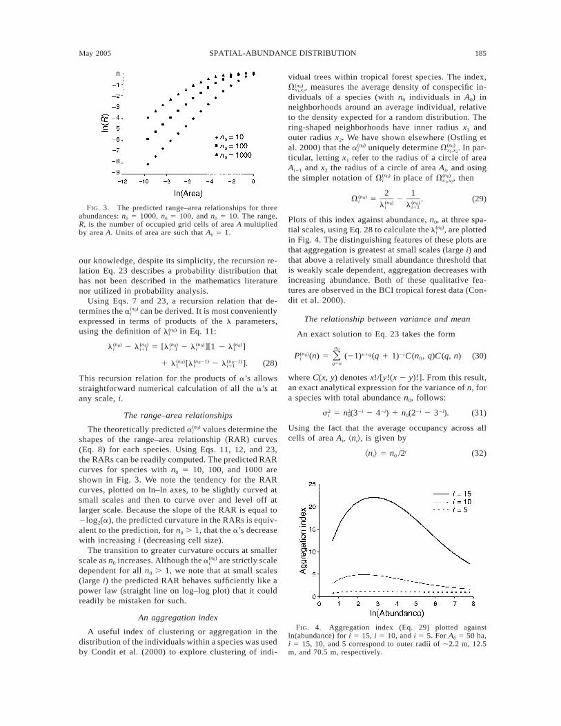
FIG. 4. Aggregation index (Eq. 29) plotted againstln(abundance) for i 5 15, i 5 10, and i 5 5. For A0 5 50 ha,i 5 15, 10, and 5 correspond to outer radii of ;2.2 m, 12.5m, and 70.5 m, respectively.

our knowledge, despite its simplicity, the recursion re-lation Eq. 23 describes a probability distribution thathas not been described in the mathematics literaturenor utilized in probability analysis.

Using Eqs. 7 and 23, a recursion relation that de-termines the can be derived. It is most conveniently(n )0ai

expressed in terms of products of the l parameters,using the definition of in Eq. 11:(n )0li

(n ) (n ) (n ) (n ) (n )0 0 0 0 0l 2 l 5 [l 2 l ][1 2 l ]i i11 i21 i 1

(n ) (n 21) (n 21)0 0 01 l [l 2 l ]. (28)1 i i11

This recursion relation for the products of a’s allowsstraightforward numerical calculation of all the a’s atany scale, i.

The range–area relationships

The theoretically predicted values determine the(n )0ai

shapes of the range–area relationship (RAR) curves(Eq. 8) for each species. Using Eqs. 11, 12, and 23,the RARs can be readily computed. The predicted RARcurves for species with n0 5 10, 100, and 1000 areshown in Fig. 3. We note the tendency for the RARcurves, plotted on ln–ln axes, to be slightly curved atsmall scales and then to curve over and level off atlarger scale. Because the slope of the RAR is equal to2log2(a), the predicted curvature in the RARs is equiv-alent to the prediction, for n0 . 1, that the a’s decreasewith increasing i (decreasing cell size).

The transition to greater curvature occurs at smallerscale as n0 increases. Although the are strictly scale(n )0ai

dependent for all n0 . 1, we note that at small scales(large i) the predicted RAR behaves sufficiently like apower law (straight line on log–log plot) that it couldreadily be mistaken for such.

An aggregation index

A useful index of clustering or aggregation in thedistribution of the individuals within a species was usedby Condit et al. (2000) to explore clustering of indi-

vidual trees within tropical forest species. The index,, measures the average density of conspecific in-(n )0Vx ,x1 2

dividuals of a species (with n0 individuals in A0) inneighborhoods around an average individual, relativeto the density expected for a random distribution. Thering-shaped neighborhoods have inner radius x1 andouter radius x2. We have shown elsewhere (Ostling etal. 2000) that the uniquely determine . In par-(n ) (n )0 0a Vi x ,x1 2

ticular, letting x1 refer to the radius of a circle of areaAi11 and x2 the radius of a circle of area Ai, and usingthe simpler notation of in place of , then(n ) (n )0 0V Vi x ,x1 2

2 1(n )0V 5 2 . (29)i (n ) (n )0 0l li i11

Plots of this index against abundance, n0, at three spa-tial scales, using Eq. 28 to calculate the , are plotted(n )0li

in Fig. 4. The distinguishing features of these plots arethat aggregation is greatest at small scales (large i) andthat above a relatively small abundance threshold thatis weakly scale dependent, aggregation decreases withincreasing abundance. Both of these qualitative fea-tures are observed in the BCI tropical forest data (Con-dit et al. 2000).

The relationship between variance and mean

An exact solution to Eq. 23 takes the form

n0(n ) n1q 2i0P (n) 5 (21) (q 1 1) C(n , q)C(q, n) (30)Oi 0

q5n

where C(x, y) denotes x!/[y!(x 2 y)!]. From this result,an exact analytical expression for the variance of n, fora species with total abundance n0, follows:

2 2 2i 2i 2i 2is 5 n (3 2 4 ) 1 n (2 2 3 ).i 0 0 (31)

Using the fact that the average occupancy across allcells of area Ai, ^ni&, is given by

i^n & 5 n /2i 0 (32)


we can write

2 i 2 is 5 [(4/3) 2 1]^n & 1 [1 2 (2/3) ]^n &.i i i (33)

Thus the variance contains terms that vary quadrati-cally and linearly with the mean occupancy, indicatingbehavior that is intermediate between the predictionderived under the assumption of self-similarity (Ban-avar et al. 1999), for which s2 ; (mean)2, and thecontinuous (Poisson) version of the random placementmodel, for which s2 ; mean. From Eqs. 32 and 33 wecan also calculate the scale dependence of the specificcombination of and ^ni& that comprises the parameter2si

k in the negative binomial distribution (NBD; Eq. 1):

2^n & 1i 5 . (34)2 is 2 ^n &i i 4 1

1 2 2 11 2 1 23 n0

Using the fact that Ai 5 A0 /2i, this can be rewritten as

2^n & 1i 5 . (35)2 log (4/3)2s 2 ^n &i i A 10 1 2 2 11 2 1 2A ni 0

For sufficiently large A0 /Ai and n0, this expression ap-proaches (Ai /A0)0.42, where we have used log2(4/3) ù0.42. In practice, for n0 . 10 and i . 8, this ought tobe a good approximation. This implies that the effectivevalue of the NBD parameter, k, in our theory scales asA0.42 for large i.

COMMUNITY PROPERTIES

To derive theoretical expressions for community-levelpatterns, including the species–area relationship (SAR),endemics–area relationship (EAR), and the scale-depen-dent species-abundance distribution, Fi(n), we need onlyassume that HEAP applies to all species; no assumptionsare needed about spatial correlations between speciesbecause these community-level properties depend onlyon the collection of species-level spatial distributionsand are independent of interspecific correlations. To de-rive the scale-dependent community-level spatial-abun-dance distribution, Fi(N), we additionally assume thatthe spatial distribution of the individuals in each speciesis independent of the locations of individuals in the otherspecies; in other words, HEAP applies independently toeach of the species and thus interspecific spatial corre-lations are absent.

The species–area and the endemics–arearelationships

The SAR can be expressed either in terms of the l’s,as shown in Eq. 10, or equivalently in terms of the species-level spatial distribution functions using the formula

(n )0S 5 [1 2 P (0)] (36)Oi i

where the sum is over all species. Eq. 36 states thatthe expected number of species in an Ai cell equals the

sum over species of the probability of species occur-rence in that cell, with the probability of occurrenceequal to 1 minus the probability of absence. Becausethe Pi’s and the l’s depend only on n0, the shape of theSAR is predicted uniquely in terms of the list of abun-dances n0. Although we cannot write down a simpleanalytical form for the SAR in terms of the list ofabundances (because neither Eq. 23 nor Eq. 28 has, toour knowledge, a simple closed form analytical solu-tion), we can solve for the SAR numerically from thelist of abundances using Eqs. 10 and 28, or equivalentlyEqs. 30 and 36.

A simple analytic expression for the EAR can bederived from the theory. We define a species (from thelist in A0) to be endemic to an Ai cell if all its individualsare found only in that Ai cell. Consider a single cell ofarea Ai. We seek the mean number of species that arefound only in such a cell and not within the other 2i

2 1 Ai cells that comprise A0. The dependence of thatnumber on area Ai is what we mean by an EAR. De-noting by Ei the expected number of endemic speciesin Ai, we have, from the definition of endemicity,

(n )0E 5 P (n ) (37)Oi i 0

where the sum is over all species.But from Eq. 23 it is straightforward to show that

1(n )0P (n ) 5 (38)i 0 i(n 1 1)0

and hence the EAR takes the form

1E 5 (39)Oi i(n 1 1)0

with the sum taken over all species. We note that Eq.39 yields E0 5 S 1 5 S0, as it must because all thespecies are endemic to A0 by our definition of ende-micity.

Scale-dependent species-abundance distribution

As illustrated in Fig. 1, the scale-dependent species-abundance distribution Fi(n) is given by

(n )0P (n)O i(n )0F 5 . (40)i S0

The argument of the function Fi(n) can take on valuesranging from 0 to the largest value of n0 in the com-munity and the summation in Eq. 40 is taken over allspecies.

Community-level spatial-abundance distribution

The theory also yields expressions for the commu-nity-level spatial-abundance distribution, F(N), provid-ed that we assume HEAP applies independently to allspecies. In particular, the distribution of the total num-ber of individuals (that is, summed over species) overthe grid cells is given by the following:


F (N ) 5 P (n )d N, n (41)O P Oi i j j1 2∀n j( j )

where P denotes a product over all species. Here n(j)

is an abundance variable for the jth species and theequation simply states that the probability of a total ofN individuals in an Ai cell is given by the sum overthe joint probabilities for all the various combinationsof individual species abundances that add up to thevalue N.

COMPARISONS WITH DATA

The primary data set against which we test the the-oretical predictions is census data from serpentinegrassland habitat at Little Blue Ridge (Green et al.2003) located at the University of California’s Ho-mestake Mine/Donald and Sylvia McLaughlin NaturalReserve (388519 N; 1228249 W). We counted all indi-viduals of all plant species in all 256 1/4-m2 grid cellscomprising an 8 m 3 8 m plot. Our completed data setconsists of the locations at a resolution of 1/4-m2 cellsof 37 182 individuals, divided among 24 species. Fromthose data, aggregations at larger scale are readily com-puted.

We also tested the HEAP predictions using spatiallyexplicit data on tree locations in the 500 m 3 1000 mtropical forest plot at Barro Colorado Island (BCI) inPanama (Hubbell and Foster 1983, Condit et al. 1996a,Condit 1998) and in a 220 m 3 440 m dry forest plotat San Emilio (SanEm) in Costa Rica (Enquist et al.1999). The latter plot is the largest 1 3 2 shaped plotcontained within a larger, but irregularly shaped, plotin which tree census data are available. For these plots,the coordinates of every individual in every tree specieswith dbh $1 cm is recorded. The BCI data set contains235 308 individuals divided among 305 species and thedry forest data set contains 12 851 individuals dividedamong 138 species. For all three sites, the empiricalspecies-level and community-level distributions arecomputed from data on all 2i Ai cells, and thus the SARand EAR are derived from a complete nested analysis.

Where appropriate, we calculate 95% confidence in-tervals on linear regression slopes of predicted vs. ob-served measures, and we use a likelihood-ratio test tocompare the HEAP model predictions to those fromdistributions that fall along the continuum from randomto maximally aggregated as defined by Eq. 27. To sim-ply express the explanatory power of HEAP we use R2

values to quantify the fraction of variance in the datathat is explained by HEAP. In our comparisons to arandom model, we use the random placement model ofColeman (1981), in which individuals from a specifiedspecies-abundance distribution are at every scaleplaced on a gridded landscape according to a binomialdistribution. We emphasize that our goal is not the im-possible task of establishing the superiority of HEAPrelative to all other theories; rather it is to show theextent to which it captures the ecologically significant

features of numerous spatial patterns and to identifythe dominant trends in its failures to fit all the detailsof empirical patterns.

The species-level spatial distributionsand the a parameters

A test of Eq. 23, the fundamental species-level pre-diction of HEAP, consists of comparing the observedand predicted spatial-abundance distributions. Quali-tatively, the spatial-abundance distributions are mono-tonically decreasing for nearly all species at the threesites across the range of scales examined here; thus forn0 . 2i they differ from the hump-shaped predictionsexpected from the random (binomial distribution) mod-el. To see if the HEAP prediction captures the quan-titative features of the data, we compare the actualshapes of the (n) to the data. These comparisons(n )0Pi

are carried out at scale i 5 6 and 8 for the serpentinedata and at i 5 8 and 15 for the BCI and San Emiliodata. The scale i 5 15 corresponds to 15-m2 quadrats,with a mean of 7 individuals in each, at BCI, and 3-m2 quadrats, with a mean of 0.4 individuals in each, atSan Emilio. The scale i 5 8 corresponds to 0.25-m2

quadrats, with a mean of 144 individuals in each, atthe serpentine site; this is the smallest scale censusedat that site.

Fig. 5 shows predicted and empirical values of thespatial-abundance distributions for four serpentine spe-cies with abundances ranging from n0 5 49 to 3095.These species represent the range of abundances pres-ent in the data set, but were otherwise randomly se-lected. For the two most abundant species shown, therandom model prediction at i 5 6 is ;0 over the rangeof abundances plotted and does not even show up inthe figure. We note three qualitative features of thesecomparisons. (1) The HEAP predictions match the gen-eral shape of the observed distributions and outperformthe random model predictions at both scales and forall four species. (2) The differences between HEAPand random predictions diminish, but do not becomenegligible, with decreasing abundance. (3) As abun-dance increases, the HEAP prediction increasingly ov-erpredicts the fraction, (0), of unoccupied cells.(n )0Pi

Equivalently, it tends to overpredict the abundances ofoccupied cells and thus the level of aggregation. Al-though not shown in the figure, the spatial distributiondata are also well described by HEAP for the verylowest-abundance species (n0 , 30).

Comparisons of theory and observation reveal thesame three features for the BCI tropical forest data set(Fig. 6) and the San Emilio data set (Fig. 7) at scalesi 5 8 and 15, except that feature (3) is no longer trueat i 5 15. In particular, the HEAP prediction for (0)(n )0Pi

matches the data well for all abundances at that finescale. Accurate prediction of the values of (0) at(n )0Pi

fine scales implies accurate prediction of the values ofthe a’s at those scales. For both these tropical sites,the species tested in Figs. 6 and 7 were chosen to have


FIG. 5. Observed and predicted species-level distributions (n), multiplied by 2i to yield the expected number of cells(n )0Pi

occupied with n individuals for the serpentine plot. The abundances of the species selected for comparison and the scalesof analysis are shown in the figures; the four species represent the range of abundances but were otherwise randomly selected.Random model predictions are from the Coleman (1981) random placement model; random model predictions for n0 5 617and 3095 are not shown at scale i 5 6 because they are ;0 over the range of n values plotted.

FIG. 6. Same as Fig. 5 for the BCI site, except that scales i 5 8 and 15 are plotted. The species were chosen to haveabundances closest to those in Fig. 5.

abundances closest to the four species selected fromthe serpentine site, although at the San Emilio site thereare no species with n0 . 1000.

By focusing on the parameters, we can gain a(n )0ai

more detailed picture of the tendency for Eq. 23 tooverpredict the amount of aggregation in the distri-butions of the higher-abundance species. A graph ofpredicted vs. measured values, averaged over(n )0ai

scales i 5 4, 6, and 8, for all the species in the ser-pentine plot, shows generally good agreement, but ageneral tendency for HEAP to underpredict the a’s ofthe species with the highest a values (Fig. 8a). Becauseat any given scale, the predicted value of is a(n )0ai

monotonic increasing function of n0, this implies atrend toward underprediction of a for the higher-abun-dance species. This is consistent with the general trend


FIG. 7. Same as Fig. 6 for the San Emilio site, except that no species at the San Emilio site had n0 . 1000.

FIG. 8. Comparison of observed and predicted values of for all plant species in (a) the serpentine plot, (b) the BCI(n )0ai

plot, and (c) the San Emilio site. Comparisons are averaged over scales i 5 4, 6, and 8. The dashed line is the one-to-oneline, and the solid line is the linear regression of predicted on measured values. Solid squares are the HEAP predictions, andopen triangles are predicted values of the from the random placement model (Coleman 1981), calculated from the(n )0ai

measured abundances, n0.

that we saw in Figs. 5–7 for HEAP to overpredict(0) for the higher-abundance species. The slope of(n )0Pi

the linear regression (solid line in figure) is 0.91 with95% confidence limits of (0.80, 1.02). For each species,Fig. 8a also shows the predicted value of a, averagedover the same scales, from the random model. We notethat compared to HEAP and to the data, the randommodel underpredicts the a’s at small abundance andoverpredicts them at large abundance. To assess therelative performance of HEAP and the random model,we compare the ratio of sum of squared errors (RSSE)of each model using the ratio

2ˆ(Y 2 Y )O randomRSSE 5 (42)

2ˆ(Y 2 Y )O HEAP

where the sums are over species, Y are the observedvariables, and Y are the random or HEAP model pre-

dictions. RSSE . 1 implies that HEAP fits the observeddata better than the random model. The calculatedRSSE for the serpentine data in Fig. 8a is 2.9.

For each of the scales i 5 1, 2, 4, 6, 8, the fractionsof variance in the serpentine a data that are explainedby HEAP (the squared correlations between the HEAP-predicted values and the measured values) are 0.70,0.79, 0.74, 0.92, and 0.94, respectively. We note thateven at scale i 5 1, where the distribution of individualsbetween the right and left halves of the 64-m2 plot areexamined, HEAP explains 70% of the variance in thea’s, but that the explained variance increases at finerscales.

The HEAP predictions for the a’s at the BCI andSan Emilio sites are not as accurate as at the serpentinesite (Fig. 8b,c). The slopes of the linear regressions ofpredicted against measured a values are 0.75 and 0.73,


FIG. 9. Comparison of observed and predicted values ofabundance for the serpentine species. The HEAP predictionsfor abundance are derived by calculating the value of n0 thatyields, from Eq. 7, a value of a8 equal to the measured valueof a8 for each species. The HEAP prediction explains 88%of the variance in the data shown in the figure, and the slopeof the linear regression is 1.16, with 95% confidence limitsof (0.92, 1.40).

respectively, with 95% confidence intervals of 60.03and 60.05 for BCI and SanEm, respectively. HEAPexplains 93% of the variance in the a values, at eachof the forest sites. As at the serpentine site, the randommodel underpredicts the a’s at low abundance (smalla) and overpredicts the a’s at high abundance in theforest sites; the observed values of a for the high-abundance species fall between the HEAP and randommodel predictions, and with all species included, theRSSE (Eq. 42) values are ;1 at both sites.

Another way to portray the relationship between thepredicted and measured a’s is to plot actual speciesabundances, n0, against the abundances predicted fromthe measured a’s (see Theoretical background: Theprobability parameters for the discussion following Eq.8). This comparison is of practical value because thereis interest in being able to estimate overall abundanceof a species within some large area based only on anempirical estimate of cell occupancy (i.e., presence/absence data) in small cells within that large area. Fig.9 shows this comparison for the serpentine species.HEAP explains 88% of the variance in the measuredvalues of ln(n0) and the slope of the regression line inthe figure is 1.16 6 0.24 (95% CI). Fig. 9 shows thatHEAP tends to overpredict abundance (equivalent tounderpredicting a) for the higher-abundance species,consistent with Fig. 8a. We will return to this system-atic pattern of discrepancy in the HEAP predictionslater when we discuss future directions.

The mean–variance relationship

For A0 5 50 ha, corresponding to the BCI data, andexpressing A in units of m2, HEAP predicts k 5 0.004

3 A0.42 at small scales and for all but the lowest-abun-dance species (Eq. 34). This predicted scale depen-dence for the quantity k is close to the empirical findingof J. Plotkin (personal communication) that if k is writ-ten as cAw, then for the BCI species, fitted values of cand w cluster around values of ;0.003 and ;0.45,respectively.

The SAR and the EAR

Starting with the list of abundances of the speciesin A0, the can be calculated for all the species in(n )0li

a community from Eq. 28. Then, using Eq. 10, thespecies–area relationship (SAR) is determined. Equiv-alently, Eqs. 23 and 36 can be used to determine thepredicted SAR. Because of our top-down boundarycondition, in our tests of the SAR and the endemics–area relationship (EAR) the total number of predictedspecies is constrained empirically at the largest scale,A0. The theoretical prediction captures the general fea-tures of the serpentine SAR (Fig. 10a,b) but tends tounderpredict species richness at the forest sites. Thisdiscrepancy is consistent with the pattern in which thespatial distributions of the high-abundance species de-viate from the theoretical predictions: the theory un-derpredicts species richness because it overpredicts thenumber of unoccupied cells for the high-abundancespecies. Equivalently, HEAP underpredicts the a’s forthose species and thus by Eq. 9 and the relationship z5 2log2(a), it overpredicts the slope of the SAR. Wenote that the gross differences across sites in the slopesof the empirical species richness vs. ln(area) plots(slopeBCI . slopeSanEm . slopeSERP) are captured by thetheory (Fig. 10b) and that these gross differences inpredicted slopes result solely from the different lists ofspecies abundances at the three sites.

The theoretical EAR (Eq. 39) matches quite accu-rately the empirical EAR at all three sites (Fig. 11),again with no adjustable parameters. If the individualsof each species are distributed randomly, then wewould expect the following (Green and Ostling 2003):

2in0E 5 2 (43)Oi

where the sum is over all species. Compared to Eq. 39,this expression significantly underestimates the ob-served data at scales i 5 1 and 2, but fits the data aswell as our theory at smaller spatial scales. The reasonis that at small spatial scales, only species with n0 51 contribute significantly to endemism, and for thosespecies a 5 1/2 in HEAP, which is the value that arandom model would predict for those species.

The scale-dependent species-abundance distribution

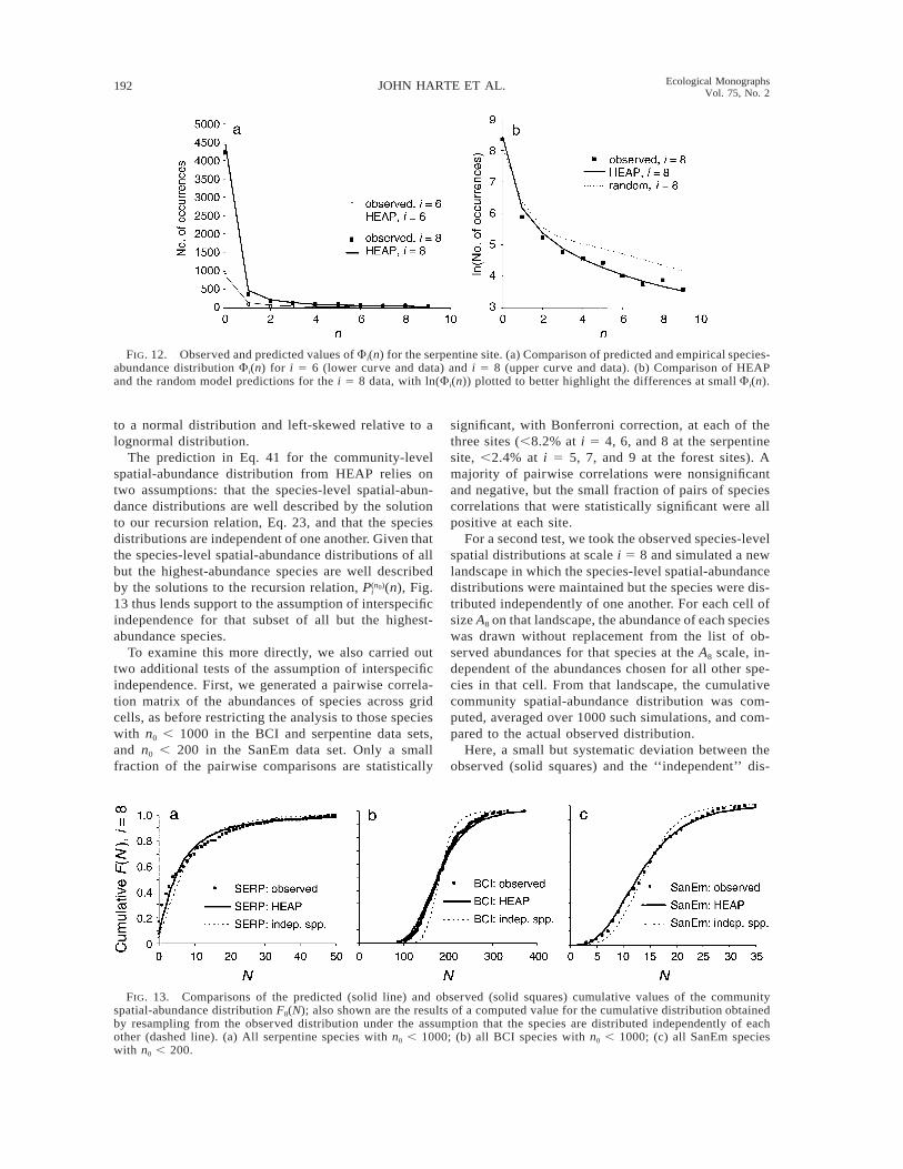
We also tested Eq. 40, the predicted expression forthe scale-dependent species-abundance distributionFi(n) for the serpentine data at i 5 6 and 8 scales (Fig.12a). At both scales the empirical cumulative distri-bution is very well described by the theoretical pre-


FIG. 10. Observed and predicted values of species richness as a function of scale for the three sites. (a) Predicted vs.observed species–area relationship (SAR); the straight line is a 1:1 line. (b) Predicted and observed species richness vs.ln(area); area is measured in square meters. Error bars on the serpentine data in panel (a) are 61 SE; error bars on the BCIand San Emilio forest data points are generally no larger than the symbols and are not shown.

FIG. 11. Observed and predicted values of endemic spe-cies richness as a function of scale for the three sites. Thestraight line is a 1:1 line.

diction. The random placement model underpredictsFi(n) at n 5 0 and overpredicts the distribution at largern, by approximately a factor of 2 relative to the dataand to HEAP (Fig. 12b). As with all our other tests oftheory here, the comparisons in Fig. 12 are not bestfits, for there are no adjustable parameters.

The community-level spatial-abundance distribution

Calculation of the full expression for the community-level spatial-abundance distribution, Fi(N), directlyfrom Eq. 41 is a difficult numerical task for values ofN $ 5 because of the huge number of combinations ofabundance values that can add up to a selected valueof N, even for just the 24 species in the serpentine plot;it becomes enormously difficult for the more species

rich forest plots. Hence we have simulated landscapesusing HEAP and then calculated the predicted Fi(N)directly from those landscapes. To verify the accuracyof the simulations, we compared simulated Fi(N) withthe exact theoretical Fi(N) calculated from Eq. 41 fori 5 6 and 8, and for N 5 0 . . . 4, using a species-abundance distribution identical to that of the serpen-tine site. The simulated Fi(N) were in excellent agree-ment with the exact theoretical results.

We carried out two types of comparison of theorywith observation; first with all the species at each site,and second using just those species with n0 , 1000 atthe serpentine and BCI plots and with n0 , 200 at theSanEm site. The second case, with restricted abun-dance, was examined because we have seen that thetheoretical species-level spatial-abundance distribu-tions do not describe well the empirical distributionsfor those species with the very highest abundances; wechose the abundance cutoff at SanEm to be 1/5 that atthe BCI plot because the area of the SanEm plot is ;1/5 that of the BCI plot. These restrictions leave us with17 out of 24 species in the serpentine community, 259out of 305 BCI species, and 116 out of 138 SanEmspecies. Although these restrictions exclude only a mi-nority of the species, they exclude a majority of theindividuals in the entire study areas.

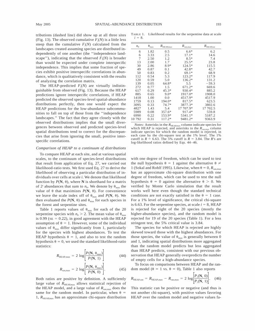
For each of the three sites, the theoretical predictionfor the cumulative community-level spatial-abundancedistribution, F8(k), agrees closely with the dataNOk50

when abundances are restricted; see the comparison ofsolid squares (data) with solid line (HEAP prediction)in Fig. 13. On the other hand, if all species are included,then the theoretical prediction rises faster at small Nand reaches a plateau at lower N than the observedcumulative distribution. We note that the predictedcommunity-level spatial-abundance distribution, Fi(N), isa hump-shaped function that is right-skewed relative


FIG. 12. Observed and predicted values of Fi(n) for the serpentine site. (a) Comparison of predicted and empirical species-abundance distribution Fi(n) for i 5 6 (lower curve and data) and i 5 8 (upper curve and data). (b) Comparison of HEAPand the random model predictions for the i 5 8 data, with ln(Fi(n)) plotted to better highlight the differences at small Fi(n).

FIG. 13. Comparisons of the predicted (solid line) and observed (solid squares) cumulative values of the communityspatial-abundance distribution F8(N); also shown are the results of a computed value for the cumulative distribution obtainedby resampling from the observed distribution under the assumption that the species are distributed independently of eachother (dashed line). (a) All serpentine species with n0 , 1000; (b) all BCI species with n0 , 1000; (c) all SanEm specieswith n0 , 200.

to a normal distribution and left-skewed relative to alognormal distribution.

The prediction in Eq. 41 for the community-levelspatial-abundance distribution from HEAP relies ontwo assumptions: that the species-level spatial-abun-dance distributions are well described by the solutionto our recursion relation, Eq. 23, and that the speciesdistributions are independent of one another. Given thatthe species-level spatial-abundance distributions of allbut the highest-abundance species are well describedby the solutions to the recursion relation, (n), Fig.(n )0Pi

13 thus lends support to the assumption of interspecificindependence for that subset of all but the highest-abundance species.

To examine this more directly, we also carried outtwo additional tests of the assumption of interspecificindependence. First, we generated a pairwise correla-tion matrix of the abundances of species across gridcells, as before restricting the analysis to those specieswith n0 , 1000 in the BCI and serpentine data sets,and n0 , 200 in the SanEm data set. Only a smallfraction of the pairwise comparisons are statistically

significant, with Bonferroni correction, at each of thethree sites (,8.2% at i 5 4, 6, and 8 at the serpentinesite, ,2.4% at i 5 5, 7, and 9 at the forest sites). Amajority of pairwise correlations were nonsignificantand negative, but the small fraction of pairs of speciescorrelations that were statistically significant were allpositive at each site.

For a second test, we took the observed species-levelspatial distributions at scale i 5 8 and simulated a newlandscape in which the species-level spatial-abundancedistributions were maintained but the species were dis-tributed independently of one another. For each cell ofsize A8 on that landscape, the abundance of each specieswas drawn without replacement from the list of ob-served abundances for that species at the A8 scale, in-dependent of the abundances chosen for all other spe-cies in that cell. From that landscape, the cumulativecommunity spatial-abundance distribution was com-puted, averaged over 1000 such simulations, and com-pared to the actual observed distribution.

Here, a small but systematic deviation between theobserved (solid squares) and the ‘‘independent’’ dis-


TABLE 1. Likelihood results for the serpentine data at scalei 5 8.

n0 umax RHEAP,max Rran,max RHEAP,ran

6 1.82 0.5 6.6* 6.26 3.33 2.5 17.1* 14.67 2.50 1.2 8.5* 7.4

13 2.00 1.7 25.5* 23.830 2.86 8.9* 124.5* 115.549 0.87 0.1 42.8* 42.750 0.83 0.2 69.1* 68.9

112 0.54 5.3 123.2* 117.9120 0.59 5.0 136.2* 131.2139 0.05 64.8* 5.5 259.3272 0.77 1.5 671.2* 669.6617 0.29 45.3* 930.4* 885.2885 0.65 9.0* 1917.0* 1908.0

1418 1.00 0.0 4517.9* 4517.91759 0.13 194.0* 817.5* 623.53095 0.33 74.7* 3877.3* 3802.64827 1.43 5.4 17 707.9* 17 702.55989 0.08 357.6* 917.4* 559.86990 0.22 153.9* 5341.1* 5187.2

10 792 0.31 117.2* 9481.2* 9363.9

Notes: Asterisks in the RHEAP,max column indicate species forwhich HEAP is rejected, and asterisks in the Rran,max columnindicate species for which the random model is rejected, ineach case by the chi-square test at the 1% level. The 1%cutoff is R 5 6.63. The 5% cutoff is R 5 3.84. The R’s arelog-likelihood ratios defined by Eqs. 44–46.

tributions (dashed line) did show up at all three sites(Fig. 13). The observed cumulative Fi(N) is a little lesssteep than the cumulative Fi(N) calculated from thelandscapes created assuming species are distributed in-dependently of one another (the ‘‘independence land-scape’’), indicating that the observed Fi(N) is broaderthan would be expected under complete interspecificindependence. This implies that some fraction of spe-cies exhibit positive interspecific correlations in abun-dance, which is qualitatively consistent with the resultsof analyzing the correlation matrix.

The HEAP-predicted Fi(N) are virtually indistin-guishable from observed (Fig. 13). Because the HEAPpredictions ignore interspecific correlations, if HEAPpredicted the observed species-level spatial-abundancedistributions perfectly, then one would expect theHEAP predictions for the low-abundance subcommu-nities to fall on top of those from the ‘‘independencelandscapes.’’ The fact that they agree closely with theobserved distributions implies that the small diver-gences between observed and predicted species-levelspatial distributions tend to correct for the discrepan-cies that arise from ignoring the small, positive inter-specific correlations.

Comparison of HEAP to a continuum of distributions

To compare HEAP at each site, and at various spatialscales, to the continuum of species-level distributionsthat result from application of Eq. 27, we carried outlikelihood-ratio tests. We first used Eq. 27 to derive thelikelihood of observing a particular distribution of in-dividuals over cells at scale i. We denote that likelihoodfunction by P(N, u), where N is shorthand for a matrixof 2i abundances that sum to n0. We denote by umax thevalue of u that maximizes P(N, u). For conveniencewe leave the scale index off of umax and P(N, u). Wethen evaluated the P(N, u) and umax for each species inthe forest and serpentine sites.

Table 1 reports values of umax for each of the 20serpentine species with n0 . 2. The mean value of umax

is 0.99 (SE 5 0.22), in good agreement with the HEAPassumption of u 5 1. However, some of the individualvalues of umax differ significantly from 1, particularlyfor the species with highest abundances. To test theHEAP hypothesis u 5 1, and also to test the randomhypothesis u 5 0, we used the standard likelihood-ratiostatistics:

P(N, u )maxR 5 2 log (44)HEAP,max [ ]P(N, 1)

P(N, u )maxR 5 2 log . (45)ran,max [ ]P(N, 0)

Both ratios are positive by definition. A sufficientlylarge value of RHEAP,max allows statistical rejection ofthe HEAP model, and a large value of Rran,max does thesame for the random model. In particular, when u 51, RHEAP,max has an approximate chi-square distribution

with one degree of freedom, which can be used to testthe null hypothesis u 5 1 against the alternative u ±1 (Sokal and Rohlf 1995). Likewise, when u 5 0, Rran,max

has an approximate chi-square distribution with onedegree of freedom, which can be used to test the nullhypothesis u 5 0 against the alternative u . 0. Weverified by Monte Carlo simulation that the resultworks well here even though the standard technicalconditions are not exactly satisfied in the u 5 1 case.For a 1% level of significance, the critical chi-squareis 6.63. For the serpentine species, at scale i 5 8, HEAPis rejected for eight of the 20 species (mostly thehigher-abundance species), and the random model isrejected for 19 of the 20 species (Table 1). For a lessstringent test, the 5% critical value is 3.84.

The species for which HEAP is rejected are highlyskewed toward those with the highest abundances. Forthose species, the value of umax is generally between 0and 1, indicating spatial distributions more aggregatedthan the random model predicts but less aggregatedthan HEAP predicts, consistent with our previous ob-servation that HEAP generally overpredicts the numberof empty cells for a high-abundance species.

To focus on comparisons between HEAP and the ran-dom model (u 5 1 vs. u 5 0), Table 1 also reports

P (N, 0)iR 5 R 2 R 5 2 log . (46)HEAP,ran HEAP,max ran,max [ ]P (N, 1)i

This statistic can be positive or negative (and thus isnot another chi-square), with positive values favoringHEAP over the random model and negative values fa-


FIG. 14. Community likelihood estimates for a continuumof models (Eq. 43) as a function of the aggregation parameterf (Eq. 47). The log of the negative of the log-likelihoodfunction is plotted so that all comparisons can be shown onone graph. Sites, scales, and subsets of species are designatedin the figure. Diamonds and squares mark the HEAP andoptimum values of f for each curve, respectively.

voring the opposite. Table 1 shows that RHEAP,ran is pos-itive for 19 of the 20 serpentine species with n0 . 2.

Qualitatively similar results hold at the BCI and SanEmilio sites, with HEAP outperforming the randommodel for ;3/4 of the species at both sites by thelikelihood-ratio criterion. For example, at scale i 5 13at BCI, HEAP outperforms the random model for 215out of the 283 species with n0 . 1. At these forest sites,however, HEAP can be statistically rejected for a largerfraction (;2/3) of species than at the serpentine site(2/5). As at the serpentine site, species for which HEAPand/or the random model are rejected by chi-squaretests are generally the ones with highest abundance.And as at the serpentine site, those rejected speciesnearly all have a umax between 0 and 1, indicating moreaggregation than under the random model but less thanunder HEAP.

We note that statistically significant rejection ofHEAP does not imply ecologically significant failureof specific HEAP predictions such as the spatial-abun-dance distributions that result from Eq. 23. For ex-ample, RHEAP, max 5 45.3 for the serpentine species withn0 5 617, which implies a highly significant rejectionof the exact HEAP value u 5 1 at i 5 8. Yet Fig. 5indicates that HEAP captures well the essential featuresof the distribution (n). Moreover, for any given(617)Pi

species a test of the HEAP prediction for P(N, u) is amore stringent test than that of Eq. 23 because it teststhe entire landscape pattern, including correlationsacross cells, and not just the distribution of abundanceswithin a single cell.

A more comprehensive test of HEAP, and insight intothe implications of strict statistical rejection of the the-ory, are obtained by looking at the community likeli-hoods. Under the assumption that spatial distributionsare independent across species, the P(N, u) for a com-munity is the product of the P(N, u) for the specieswithin the community and hence the community loglikelihood is the sum of the log-likelihood values ofthe individual species. We compare the full communitylog likelihoods at each site, as well as the log likeli-hoods for the subset of each community that excludesthe most abundant species, in Fig. 14. Because u rangesfrom 0 to `, we compare log likelihoods against thetransformed parameter

f(u) 5 u/(1 1 u) (47)

which ranges from 0 to 1, with HEAP as the midpointat f(1) 5 1/2. And because the total number of indi-viduals and the accessible scales differ markedly ateach site, we have taken a second log to allow com-parisons across extremely different log-likelihood val-ues on a single graph. Thus we have plottedlog[2log{P(N, u)}]. The negative sign is necessarybecause P(N, u) is less than 1, and thus log{P(N, u)}is negative. Because the negative reverses the orien-tation of the graph, the maximum likelihood now oc-curs at the minimum of the graph.

The plots in Fig. 14 indicate that between the lowestpoints on the curves (at a value of f that yields max-imum likelihood) and the HEAP point at f 5 1/2, thefunction is quite flat, whereas it rises rapidly at therandom extreme (f 5 0) or the completely aggregatedextreme (f 5 1). We note that for the subcommunityof species in the serpentine and BCI communities withn0 , 1000 (the majority of species), the optimum f iscloser to the value 1/2 than for the full community. Forthat subset of the BCI community, f exceeds 1/2, in-dicating that the less abundant species are somewhatmore aggregated than predicted by HEAP, whereas forthe entire community the optimal value is less than 1/2, indicating a distribution somewhat more randomthan HEAP. Overall, the community likelihoods indi-cate that HEAP performs better than the random modeland nearly as well as the model with the u that max-imizes the community likelihood at each site. The flat-ness of the curves in Fig. 14 between f 5 1/2 and f5 umax/(1 1 umax) indicates that the small divergencefrom perfect prediction, while statistically significant,may not be ecologically significant.

DISCUSSION

Our theory is based on the hypothesis of equal al-location probabilities, which states that the allocationof the individuals that are found in an Ai21 cell to thetwo Ai cells that comprise it is governed by the simplerule that all distinct combinations (without internal per-mutations) of allocation are equally probable. Our ‘‘hy-pothesis of equal allocation probabilities’’ (HEAP)leads directly to Eq. 23, the master recursion relation


that predicts the (n), and to predictions for the spe-(n )0Pi

cies–area relationship (SAR), the endemics–area rela-tionship (EAR), and the community-level species-abundance distribution Fi(n); these predictions dependonly on the species-abundance distribution at scale i5 0, F0(n). The further assumption that HEAP appliesindependently to all the species in a community resultsin a prediction for the community-level spatial-abun-dance distribution functions Fi(N).

There are no adjustable parameters in the theory andthus none of our comparisons between theory and ob-servation involve fitting procedures. These compari-sons, carried out over a wide range of scales with datafrom a serpentine meadow and two tropical forest sites,point to a general pattern of consistency between pre-dictions and data, although significant deviations be-tween the theoretical and empirical (n) are evident(n )0Pi

for species with relatively high n0. The fact that forthose high-abundance species the theory tends to ov-erpredict the number of empty cells suggests that somedegree of intraspecific density dependence needs to beincluded in the theory. Density-dependent intraspecificregulation would tend to spread species around on thelandscape more uniformly, and thus if the theory con-tained a density correction to HEAP, the theory wouldbetter describe the spatial distributions of the high-abundance species.

Because the predicted species-level and community-level spatial-abundance distributions appear to fit thedata best when the highest-abundance species are ex-cluded, we also examined the predicted and observedSAR for the subset of species that excludes the samehigh-abundance species that were excluded in the com-parisons in Fig. 13. For all three sites, the agreementbetween predicted and observed SAR was improvedrelative to the comparisons with all species included.

We emphasize that our theory is not based on anyassumptions of self-similarity or fractality in nature.The species–area relationship predicted from HEAPmay or may not exhibit power-law behavior, dependingon the distribution of the species abundances. The pre-dicted RARs cannot exhibit power-law behavior, how-ever, because the derived a parameters must be scaledependent in our theory. The predicted scale depen-dence of the a’s is such that they decrease with in-creasing i (decreasing spatial scale), which is both theway observed a’s tend to behave and the way they mustbehave if Eq. 9 is to allow even the possibility of scale-independent values for the ai’s and thus a power-lawSAR.

Although the probability parameters, , cannot be(n )0ai

scale independent under HEAP, the conditional prob-ability statement that defines the allocation rule is, infact, scale independent. This can be most easily seenby observing that under HEAP the defined in Eq.(n )0bi

24 are independent of the scale index i (Eq. 26). Wenote that they are independent of n0 as well. Numericalevaluation of the , and thus of the occupancy prob-(n )0li

abilities, for large i, large n0, and n0 of order, or greaterthan, 2i shows that occupancy probability exhibits apower-law dependence on patch area. In contrast to theassumption of species-level self-similarity in macroe-cology (Banavar et al. 1999, Harte et al. 2001), in whichthe RARs and thus the occupancy probabilities obeyexact power-law behavior, HEAP is only asymptoti-cally scale invariant.

Rationale for the assumption of HEAP

Because HEAP makes no explicit assumptions aboutbiological mechanisms such as competition, dispersal,and density dependence, it can be considered as a kindof ‘‘null theory’’ of spatial structure. While such anassumption cannot possibly predict correctly all detailsof spatial pattern, to the extent that it leads to a widerange of testable and reliable predictions, understand-ing is advanced. Moreover, to the extent that there arepatterns in the discrepancies between observation andprediction, a null theory provides an opportunity toevaluate the role of those behaviors that are assumedaway at the outset.

We based our theory on HEAP in the same spiritthat the ‘‘hypothesis of equal a priori probabilities’’(HEAPP) is made in statistical mechanics and ther-modynamics. HEAPP is the assumption that a manyparticle system such as a gas will ‘‘visit’’ all of theaccessible states available to it in phase space withequal probability and, like HEAP, it fills the vacuumof evidence created by the absence of reasons to assumeanything more complicated. Whereas HEAPP in clas-sical statistical mechanics results in a binomial distri-bution for the numbers of distinguishable gas mole-cules in the two halves of a box, HEAP results in a flatdistribution. This difference arises because underHEAP we effectively treat individuals as indistinguish-able objects and therefore do not consider as indepen-dent allocation options the many permutations over in-dividuals within a species.

The possibility of an eventual mechanistic expla-nation for the relative success of HEAP is suggestedby the fact that the entire theory can be recast math-ematically in terms of a simple functional form of anassembly (or colonization) function, bi(1 z p, q 2 p).Direct tests of the derived functional form of the b’s(Eq. 26) could help us understand the ecological in-terpretation of the b’s and perhaps provide a moremechanistic foundation for HEAP. It is not clear to uswhether the b’s should be interpreted literally as de-scriptors of an assembly process, or whether they aresimply mathematical devices that provide an alterna-tive way to derive the consequences of HEAP, such asthe form of the (n). This is an empirical question(n )0Pi

that can be answered with data from successional sites,where the sequence of individual appearances over timeon a spatial grid can be determined.


Further tasks

Because the shape of the SAR depends only on thedistribution of abundances, n0, over the species pool,there could be one or more species-abundance distri-butions that actually result in an exact power-law SARover a finite scale range. Determination of the analyticform of such species-abundance distributions (SADs)remains to be carried out.

The mismatch between our predicted (n) and the(n )0Pi

data is in the direction (see Figs. 5–7) that suggeststhat the theory would yield improved predictions if itincorporated some degree of density-dependent damp-ing of high occupancy for the high-abundance species.This is consistent with our observation that the theorytends to underpredict species richness at intermediatescales. Stated differently, HEAP imposes slightly toomuch clustering, thus overpredicting the frequency ofempty cells. Formulation of the theory in terms of theb functions (Appendix A) is a reasonable starting pointfor modifying HEAP for the high-abundance speciesby injecting intraspecific density dependence into thetheory. Although many modifications of Eq. 26 thatcause a dampening of the ‘‘rich get richer’’ effect athigh occupancy are possible, a simple Monod-kineticstype approach would be a sensible first attempt.

The theory also leads to a recursion relationship forthe dependence of species turnover on interpatch dis-tance and on patch size given only the list of abun-dances of the species at the largest spatial scale (J.Harte, unpublished manuscript). As with our test of thecommunity-level spatial distribution functions Fi(N),in Fig. 13, tests of the predictions for species turnoverwill provide insight into how well the theory predictsentire landscape structure, as opposed to just single celldistributions. A further task is to solve these recursionrelations and compare the HEAP prediction to obser-vations.

Only plant data have been used for theory testinghere. Further tests of HEAP for taxonomic groups ofanimals, such as census data on locations of breedingbird nest sites, or spatially explicit butterfly or mammalcensus data sets, would help us understand limitationson the scope of the theory. The availability of spatiallyexplicit data sets in which all individuals are censusedwithin a large contiguous area is unfortunately limited.Although we used three such data sets to test HEAP,most data sets consist of censuses within small scat-tered subplots or along sparsely located transects with-in a larger region. Another task, then, is to use HEAPto develop improved statistical techniques for extrap-olating to landscape or biome scale the informationabout species abundance and species richness that de-rives from sparse censusing at local scale.

CONCLUSION

We have presented a theory of spatial structure inthe distribution of individuals within species and spe-

cies within ecological communities, and compared itspredictions to spatially explicit vegetation census datafrom three sites. Assuming knowledge only of the spe-cies-abundance distribution at some largest scale, thetheory predicts a diversity of measures of spatial struc-ture in these data over a range of smaller spatial scales.These measures include, at species level, the spatial-abundance distributions and the range–area relation-ships, and at community level, the species–area andendemics–area relationships, a community-level spa-tial-abundance distribution, and the smaller scale spe-cies-abundance distributions. The spatial structure ofthree spatially explicit census data sets are generallyconsistent with the theory’s predictions for these mea-sures, although a systematic pattern of failure for thehigh-abundance species is apparent.

Because this theory is based on hugely simplifiedassumptions and incorporates no explicit ecologicalprocesses, it will be of interest to develop a deeperunderstanding of why it makes successful predictions.At the same time, from the patterns in the failures ofthe predictions of this null theory, it appears possibleto identify which of the many ecological processes thatare neglected in its current formulation will need to beincorporated to improve the theory. Our analysis iden-tifies the particular need to explicitly incorporate in-traspecific carrying capacity constraints at high pop-ulation density in an improved modification of the the-ory. A mathematically equivalent formulation of thetheory in terms of an assembly (or colonization) func-tion may provide the means with which to incorporatedensity dependence and develop a mechanistic foun-dation for the theory.

ACKNOWLEDGMENTS

We thank the Class of 1935 Distinguished Professorship atUC Berkeley, the EPA STAR Fellowship Program, and theNSF Bioinformatics Postdoctoral Program for financial sup-port, and Eric Berlow, Michael Bloxham, Richard Condit,Brian Enquist, Murray Gell-Mann, Nigel Goldenfeld, AnnKinzig, William Kunin, and Joshua Plotkin for useful con-versations. Two anonymous reviewers provided constructivesuggestions for improving the manuscript. We are most grate-ful to Uthara Srinivasan for many insightful discussions.

LITERATURE CITED

Banavar, J. R., J. L. Green, J. Harte, and A. Maritan. 1999.Finite size scaling in ecology. Physical Review Letters 83:4212–4214.

Bliss, C. I., and R. A. Fisher. 1953. Fitting the negativebinomial distribution to biological data. Biometrics 9:176–200.

Brown, J., D. Mehlman, and G. Stevens. 1995. Spatial var-iation in abundance. Ecology 76:2028–2043.

Chave, J. 2004. Neutral theory and community ecology. Ecol-ogy Letters 7:241–253.

Coleman, B. 1981. On random placement and species–arearelations. Journal of Mathematical Biosciences 54:191–215.

Condit, R. 1998. Tropical forest census plots. Springer-Ver-lag, Berlin, Germany, and R. G. Landes, Georgetown, Tex-as, USA.


Condit, R., et al. 2000. Spatial patterns in the distributionof tropical tree species. Science 288:1414–1418.

Condit, R., S. P. Hubbell, and R. B. Foster. 1996a. Changesin tree species abundance in a neotropical forest: impactof climate change. Journal of Tropical Ecology 12:231–256.

Condit, R., S. P. Hubbell, J. V. LaFrankie, R. Sukumar, N.Manokaran, R. Foster, and P. S. Ashton. 1996b. Species–area and species–individual relationships for tropical trees:a comparison of three 50-ha plots. Journal of Ecology 84:549–562.

Condit, R., et al. 2002. Beta-diversity in tropical forest trees.Science 295:666–669.

Enquist, B. J., G. B. West, E. L. Charnov, and J. H. Brown.1999. Allometric scaling of production and life historyvariation in vascular plants. Nature 401:907–911.

Fisher, R., A. Corbet, and C. Williams. 1943. The relationbetween the number of species and the number of individ-uals in a random sample of an animal population. Journalof Animal Ecology 12:42–58.

Gaston, K., and T. Blackburn. 2000. Pattern and process inmacroecology. Blackwell Scientific, Oxford, UK.

Green, J., J. Harte, and A. Ostling. 2003. Species richness,endemism and abundance patterns: tests of two fractal mod-els in a serpentine grassland. Ecology Letters 6:919–928.

Green, J., and A. Ostling. 2003. Endemics–area relationships:the influence of species dominance and spatial aggregation.Ecology 84:3090–3097.

Harte, J., T. Blackburn, and A. Ostling. 2001. Self similarityand the relationship between abundance and range size.American Naturalist 157:374–386.

Harte, J., A. Kinzig, and J. Green. 1999. Self similarity inthe distribution and abundance of species. Science 284:334–336.

He, F., and K. Gaston. 2000. Estimating species abundancefrom occurrence. American Naturalist 156:553–559.

He, F., and K. Gaston. 2003. Occupancy, spatial variance,and the abundance of species. American Naturalist 162:366–375.

He, F., and S. Hubbell. 2003. Percolation theory for the dis-tribution and abundance of species. Physical Review Let-ters 91(19):198103.

He, F., and P. Legendre. 2002. Species diversity patterns de-rived from species area models. Ecology 83:1185–1198.

Hubbell, S. 2001. The unified neutral theory of biodiversityand biogeography. Monographs in population biology 32.Princeton University Press, Princeton, New Jersey, USA.

Hubbell, S. P., and R. B. Foster. 1983. Diversity of canopytrees in a neotropical forest and implications for conser-vation. Pages 25–41 in S. L. Sutton, T. C. Whitmore, andA. C. Chadwick, editors. Tropical rain forest: ecology andmanagement. Blackwell Scientific Publications, Oxford,UK.

Krebs, C. 1994. Ecology: the experimental analysis of dis-tribution and abundance. Harper Collins, New York, NewYork, USA.

Kunin, W. E. 1998. Extrapolating species abundance acrossspatial scales. Science 281:1513–1515.

Kunin, W. E., S. Hartley, and J. Lennon. 2000. Scaling down:on the challenge of estimating abundance from occurrencepatterns. American Naturalist 156:553–559.

Leibold, M. A., M. Holyoak, N. Mouquet, P. Amarasekare,J. M. Chase, M. F. Hoopes, R. D. Holt, J. B. Shurin, R.Law, D. Tilman, M. Loreau, and A. Gonzalez. 2004. Themetacommunity concept: a framework for multi-scale com-munity ecology. Ecology Letters 7(7):601–613.

May, R. M. 1975. Patterns of species abundance and diver-sity. Pages 81–120 in M. L. Cody and J. M. Diamond,editors. Ecology and evolution of communities. BelknapPress, Cambridge, Massachusetts, USA.

May, M., J. Lawton, and N. Stork. 1995. Assessing extinctionrates. Pages 1–24 in J. H. Lawton and R. M. May, editors.Extinction rates. Oxford University Press, Oxford, UK.

McGill, B., and C. Collins. 2003. A unified theory for ma-croecology based on spatial patterns of abundance. Evo-lutionary Ecology Research 5:469–492.

Ostling, A., J. Harte, and J. Green. 2000. Self-similarity andclustering in the spatial distribution of species. Technicalcomment. Science 290:671a.

Ostling, A., J. Harte, J. Green, and A. Kinzig. 2003. A com-munity-level fractal property produces power-law species–area relationships. Oikos 103:218–224.

Ostling, A., J. Harte, J. Green, and A. Kinzig. 2004. Selfsimilarity, the power-law form of the species–area rela-tionship, and a probability rule: a reply to Maddux. Amer-ican Naturalist 163:627–633.

Pielou, E. C. 1969. An introduction to mathematical ecology.J. Wiley and Sons, New York, New York, USA.

Plotkin, J., and H. Muller-Landau. 2002. Sampling the spe-cies composition of a landscape. Ecology 83:3344–3356.

Plotkin, J., M. Potts, N. Leslie, N. Manokaran, J. LaFrankie,and P. Ashton. 2000. Species-area curves, spatial aggre-gation, and habitat specialization in tropical forests. Journalof Theoretical Biology 207:81–99.

Preston, F. 1948. The commonness, and rarity, of species.Ecology 84:549–562.

Preston, F. W. 1962. The canonical distribution of common-ness and rarity. Part I. Ecology 43:185–215.

Rosenzweig, M. 1995. Species diversity in space and time.Cambridge University Press, Cambridge, UK.

Ruhla, C. 1992. The physics of chance. Oxford UniversityPress, Oxford, UK.

Sokal, R. R., and F. J. Rohlf. 1995. Biometry: the principlesand practice of statistics in biological research. Third edi-tion. W. H. Freeman, New York, New York, USA.

Whitmore, T., and J. Sayer. 1992. Tropical deforestation andspecies extinction. Chapman and Hall, London, UK.

Wright, D. 1991. Correlations between incidence and abun-dance are expected by chance. Journal of Biogeography 18:463–466.

APPENDIX

Derivation of the hypothesis of equal allocation probabilities (HEAP) from an assembly function is available in ESA’sElectronic Data Archive: Ecological Archives M075-007-A1.

A theory of spatial structure in ecological communities at multiple spatial scales

Documents

Transcript of A theory of spatial structure in ecological communities at multiple spatial scales