Optimal measurement of visual motionacross spatial and temporal scales

Sergei Gepshtein1 and Ivan Tyukin2,3

1 Systems Neurobiology Laboratories, Salk Institute for Biological Studies10010 North Torrey Pines Road, La Jolla, CA 92037, USA

sergei@salk.edu

2 Department of Mathematics, University of LeicesterUniversity Road, Leicester LE1 7RH, UK

i.tyukin@le.ac.uk

3 Department of Automation and Control ProcessesSaint-Petersburg State Electrotechnical University

5 Professora Popova Str., 197376, Saint-Petersburg, Russia

April 26, 2014

Abstract. Sensory systems use limited resources to mediate the percep-tion of a great variety of objects and events. Here a normative frameworkis presented for exploring how the problem of efficient allocation of re-sources can be solved in visual perception. Starting with a basic propertyof every measurement, captured by Gabor’s uncertainty relation aboutthe location and frequency content of signals, prescriptions are developedfor optimal allocation of sensors for reliable perception of visual motion.This study reveals that a large-scale characteristic of human vision (thespatiotemporal contrast sensitivity function) is similar to the optimalprescription, and it suggests that some previously puzzling phenomenaof visual sensitivity, adaptation, and perceptual organization have simpleprincipled explanations.

Keywords: resource allocation, contrast sensitivity, perceptual organi-zation, sensory adaptation, automated sensing

Table of Contents

Optimal measurement of visual motion across spatial and temporal scales 1Sergei Gepshtein and Ivan Tyukin

1 Introduction . . . . . . . . . . . . . . . . . . . . . . . . . . . . . . . . . . . . . . . . . . . . . . . . . . . 22 Gabor’s uncertainty relation in one dimension . . . . . . . . . . . . . . . . . . . . . 5

2.1 Single sensors . . . . . . . . . . . . . . . . . . . . . . . . . . . . . . . . . . . . . . . . . . . . . 52.2 Sensor populations . . . . . . . . . . . . . . . . . . . . . . . . . . . . . . . . . . . . . . . . 72.3 Cooperative measurement . . . . . . . . . . . . . . . . . . . . . . . . . . . . . . . . . . 9

3 Gabor’s uncertainty in space-time . . . . . . . . . . . . . . . . . . . . . . . . . . . . . . . . 103.1 Uncertainty in two dimensions . . . . . . . . . . . . . . . . . . . . . . . . . . . . . . 103.2 Equivalence classes of uncertainty . . . . . . . . . . . . . . . . . . . . . . . . . . . 113.3 Spatiotemporal interaction: speed . . . . . . . . . . . . . . . . . . . . . . . . . . . 13

4 Optimal conditions for motion measurement . . . . . . . . . . . . . . . . . . . . . . . 154.1 Minima of uncertainty . . . . . . . . . . . . . . . . . . . . . . . . . . . . . . . . . . . . . 154.2 The shape of optimal set . . . . . . . . . . . . . . . . . . . . . . . . . . . . . . . . . . . 16

5 Sensor allocation . . . . . . . . . . . . . . . . . . . . . . . . . . . . . . . . . . . . . . . . . . . . . . . 185.1 Adaptive allocation . . . . . . . . . . . . . . . . . . . . . . . . . . . . . . . . . . . . . . . . 185.2 Mechanism of adaptive allocation . . . . . . . . . . . . . . . . . . . . . . . . . . . . 205.3 Conclusions . . . . . . . . . . . . . . . . . . . . . . . . . . . . . . . . . . . . . . . . . . . . . . . 21

6 Appendices . . . . . . . . . . . . . . . . . . . . . . . . . . . . . . . . . . . . . . . . . . . . . . . . . . . 256.1 Appendix 1. Additivity of uncertainty . . . . . . . . . . . . . . . . . . . . . . . . 256.2 Appendix 2. Improving resolution by multiple sampling . . . . . . . . 26

1 Introduction

Biological sensory systems collect information from a vast range of spatial andtemporal scales. For example, human vision can discern modulations of lumi-nance that span nearly seven octaves of spatial and temporal frequencies, whilemany properties of optical stimulation (such as the speed and direction of mo-tion) are analyzed within every step of the scale.

The large amount of information is encoded and transformed for the sake ofspecific visual tasks using limited resources. In biological systems, it is a large butfinite number of neural cells. The cells are specialized: sensitive to a small subsetof optical signals, presenting sensory systems with the problem of allocation oflimited resources. This chapter is concerned with how this problem is solvedby biological vision. How are the specialized cells distributed across the greatnumber of potential optical signals in the environments that are diverse andvariable?

The extensive history of vision science suggests that any attempt of visiontheory should begin with an analysis of the tasks performed by visual systems.Following Aristotle, one may begin with the definition of vision as “knowing hat

Introduction

is where by looking” [1]. The following argument concerns the basic visual taskscaptured by this definition.

The “what” and “where” of visual perception are associated with two char-acteristics of optical signals: their frequency content and locations, in space andtime. The last statement implicates at least five dimensions of optical signals(which will become clear in a moment).

The basic visual tasks are bound by first principles of measurement. To seethat, consider a measurement device (a “sensor” or “cell”) that integrates itsinputs over some spatiotemporal interval. An individual device of an arbitrarysize will be more suited for measuring the location or the frequency contentof the signal, reflected in the uncertainties of measurement. The uncertaintiesassociated with the location and the frequency content are related by a simplelaw formalized by Gabor [2], who showed that the two uncertainties trade offacross scales. As the scale changes, one uncertainty rises and the other falls.

Assuming that the visual systems in question are interested in both thelocations and frequency content of optical signals (“stimuli”), the tradeoff ofuncertainties will attain a desired (“optimal”) balance of uncertainties at someintermediate scale. The notion of the optimal tradeoff of uncertainty has re-ceived considerable attention in studies of biological vision. This is because the“receptive fields” of single neural cells early in the visual pathways appear toapproximate one or another form of the optimal tradeoff [3–10].

Here the tradeoff of uncertainties is formulated in a manner that is helpfulfor investigating its consequences outside of the optimum: across many scales,and for cell populations rather than for single cells. Then the question is posedof how the scales of multiple sensory cells should be selected for simultaneouslyminimizing the uncertainty of measurement for all the cells, on several stimulusdimensions.

The present focus is on how visual motion can be estimated at the low-est overall uncertainty of measurement across the entire range of useful sensorsizes (in artificial systems) or the entire range of receptive fields (in biologicalsystems). In other words, the following is an attempt to develop an economicnormative theory of motion-sensitive systems. Norms are derived for efficient de-sign of such systems, and then the norms are compared with facts of biologicalvision.

This approach from first principles of measurement and parsimony helps tounderstand the forces that shape the characteristics of biological vision, butwhich had appeared intractable or controversial using previous methods. Thesecharacteristics include the spatiotemporal contrast sensitivity function, adap-tive transformations of this function caused by stimulus change, and also somecharacteristics of the higher-level perceptual processes, such as perceptual orga-nization.

3

Introduction

A

C

B

Sp

atia

lfr

equ

ency

f x

Measurement interval �x

Un

cert

ain

ty

Uf

U = U + Uj x f

Ux

Location x

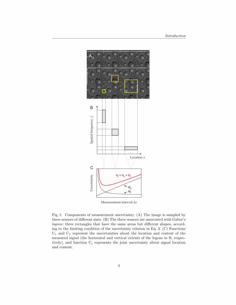
Fig. 1: Components of measurement uncertainty. (A) The image is sampled bythree sensors of different sizes. (B) The three sensors are associated with Gabor’slogons: three rectangles that have the same areas but different shapes, accord-ing to the limiting condition of the uncertainty relation in Eq. 3. (C) FunctionsUx and Uf represent the uncertainties about the location and content of themeasured signal (the horizontal and vertical extents of the logons in B, respec-tively), and function Uj represents the joint uncertainty about signal locationand content.

4

Gabor’s uncertainty in one dimension

2 Gabor’s uncertainty relation in one dimension

The outcomes of measuring the location and the frequency content of any signalby a single sensory device are not independent of one another. The measurementof location assigns the signal to interval ∆x on some dimension of interest x.The smaller the interval the lower the uncertainty about signal location. Theuncertainty is often described in terms of the precision of measurements, quan-tified by the dispersion of the measurement interval or, even simpler, by the sizeof the interval, ∆x. The smaller the interval, the lower the uncertainty aboutlocation, and the higher the precision of measurement.

The measurement of frequency content evaluates how the signal varies over x,i.e., the measurement is best described on the dimension of frequency of signalvariation, fx. That is, the measurement of frequency content is equivalent tolocalizing the signal on fx: assigning the signal to some interval ∆fx. Again, thesmaller the interval, the lower the uncertainty of measurement and the higherthe precision.4

The product of uncertainties about the location and frequency content of thesignal is bounded “from below” [2, 11–13]. The product cannot be smaller thansome positive constant Cx:

UxUf ≥ Cx, (1)

where Ux and Uf are the uncertainties about the location and frequency contentof the signal, respectively, measured on the intervals ∆x and ∆fx.

Eq. 1 means that any measurement has a limit at UxUf = Cx. At the limit,decreasing one uncertainty is accompanied by increasing the other. For simplic-ity, let us quantify the measurement uncertainty by the size of the measurementinterval. Gabor’s uncertainty relation may therefore be written as

∆x∆fx ≥ Cx, (2)

and its limiting condition as

∆x∆fx = Cx. (3)

2.1 Single sensors

Let us consider how the uncertainty relation constrains the measurements bya single measuring device: a “sensor.” Fig 1 illustrates three spatial sensors ofdifferent sizes. In Fig 1A, the measurement intervals of the sensors are defined ontwo spatial dimensions. For simplicity, let us consider just one spatial dimension,x, so the interval of measurement (“sensor size”) is ∆x, as in Fig 1B–C.

The limiting effect of the uncertainty relation for such sensors has a con-venient graphic representation called “information diagram” (Fig 1B). Let thetwo multiplicative terms of Eq. 3 be represented by the two sides of a rectanglein coordinate plane (x, fx). Then Cx is the rectangle area. Such rectangles arecalled “information cells” or “logons.” Three logons, of different shapes but ofthe same area Cx, are shown in Fig 1B, representing the three sensors:

4 For brevity, here “frequency content” will sometimes be shortened to “content.”

5

Gabor’s uncertainty in one dimension

– The logon of the smallest sensor (smallest ∆x, left) is thin and tall, indicatingthat the sensor has a high precision on x and a low precision on fx.

– The logon of the largest sensor (right) is thick and short, indicating a lowprecision on x and a high precision on fx.

– The above sensors are specialized for measuring either the location or fre-quency content of signals. The medium-size sensor (middle) offers a compro-mise: its uncertainties are not as low as the lowest uncertainties (but not ashigh as the highest uncertainties) of the specialized sensors. In this respect,the medium-size sensor trades one kind of uncertainty for another.

The medium-size sensors are most useful for jointly measuring the locations andfrequency content of signals.

So far, the ranking of sensors has been formalize using an additive model ofuncertainty (Fig 1C). The motivation for such an additive model is presented inAppendix 1. This approach is motivated by the assumption that visual systemshave no access to complete prior information about the statistics of measuredsignals (such as the joint probability density functions for the spatial and tempo-ral locations of stimuli and their frequency content). The assumption is, instead,that the systems can reliably estimate only the means and variances of the mea-sured quantities.

Accordingly, the overall uncertainty in Fig 1C has the following components.The increasing function represents the uncertainty about signal location: Ux =∆x. The decreasing function represents the uncertainty about signal content:Uf = ∆fx = Cx/∆x (from Eq. 3). The joint uncertainty of measuring signallocation and content is represented by the non-monotonic function Uj :

Uj = λxUx + λfUf = λx∆x+ λf1

∆x, (4)

where λx and λf are positive coefficients reflecting how important the compo-nents of uncertainty are relative to one another.

The additive model of Eq. 4 implements a worst-case estimate of the overalluncertainty (as it is explained in section The Minimax Principle just below). Theadditive components are weighted, while the weights are playing several roles.They bring the components of uncertainty to the same units, allowing for differ-ent magnitude of Cx,5 and representing the fact that the relative importance ofthe components depends on the task at hand.

The joint uncertainty function (Uj in Fig 1C) has its minimum at an inter-mediate value of ∆x. This is a point of equilibrium of uncertainties, in that asensor of this size implements a perfect balance of uncertainties about the lo-cation and frequency content of the signal [14]. If measurements are made inthe interest of high precision, and if the location and the frequency content ofthe signal are equally important, then a sensor of this size is the best choice forjointly measuring the location and the frequency content of the signal.

5 Different criteria of measurement and sensor shapes correspond to different magni-tudes of Cx.

6

Gabor’s uncertainty in one dimension

The Minimax Principle. What is the best way to allocated resources in orderto reduce the chance of gross errors of measurement. One approach to solvingthis problem is using the minimax strategy devised in game theory for modelingchoice behavior [15, 16]. Generally, the minimax strategy is used for estimatingthe maximal expected loss for every choice and then pursuing the choices, forwhich the expected maximal loss is minimal. In the present case, the choice isbetween the sensors that deliver information with variable uncertainty.

In the following, the minimax strategy is implemented by assuming the maxi-mal (worst-case) uncertainty of measurement on the sensors that span the entirerange of the useful spatial and temporal scales. This strategy is used in twoways. First, the consequences of Gabor’s uncertainty relation are investigatedby assuming that the uncertainty of measurement is as high as possible (i.e.,using the limiting case of uncertainty relation; Eq. 3). Second, the outcomesof measurement on different sensors are anticipated by adding their componentuncertainties, i.e., using the joint uncertainty function of Eq. 4. (The choice ofthe additive model is explained in Appendix 1.) It is assumed that sensor prefer-ences are ranked according to the expected maximal uncertainty: the lower theuncertainty, the higher the preference.

2.2 Sensor populations

Real sensory systems have at their disposal large but limited numbers of sensors.Since every sensor is useful for measuring only some aspects of the stimulus,sensory systems must solve an economic problem: they must distribute theirsensors in the interest of perception of many different stimuli. Let us considerthis problem using some simple arrangements of sensors.

First, consider a population of identical sensors in which the measurementintervals do not overlap. Fig 2A contains three examples of such sensors, usingthe information diagram introduced in Fig 1. Each of the three diagrams inFig 2A portrays four sensors, identical to one another except they are tuned todifferent intervals on x (which can be space or time). Each panel also containsa representation of a narrow-band signal: the yellow circle, the same across thethree panels of Fig 2A. The different arrangements of sensors imply differentresolutions of the system for measuring the location and frequency content ofthe stimulus.

– The population of small sensors (small ∆x on the left of Fig 2A) is most suit-able for measuring signal location: the test signal is assigned to the rightmostquarter on the range of interest in x. In contrast, measurement of frequencycontent is poor: signals presented anywhere within the vertical extent of thesensor (i.e., within the large interval on fx) will all give the same response.This system has a good location resolution and poor frequency resolution.

– The population of large sensors (large ∆x on the right of Fig 2A) is mostsuitable for measuring frequency content. The test signal is assigned to asmall interval on fx. Measurement of location is poor. This system has agood frequency resolution and poor location resolution.

7

Gabor’s uncertainty in one dimension

Fig. 2: Allocation of multiple sensors. (A) Information diagrams for a popula-tion of four sensors, using sensors of the same size within each population, and ofdifferent sizes across the populations. (B) Uncertainty functions. The red curveis the joint uncertainty function introduced in Fig 1, with the markers indicat-ing special conditions of measurement: the lowest joint uncertainty (the circle)and the equivalent joint uncertainty (the squares), anticipating the optimal setsand the equivalence classes of measurement in the higher-dimensional systemsillustrated in Figs 3–4. (C) Preference functions. The solid curve is a functionof allocation preference (here reciprocal to the uncertainty function in B): anoptimal distribution of sensors, expected to shift (dashed curve) in response tochange in stimulus usefulness.

8

Gabor’s uncertainty in one dimension

– The population of medium-size sensors can obtain useful information aboutboth locations and frequency content of signals. It has a better frequency res-olution than the population of small sensors, and a better location resolutionthan the population of large sensors.

Consequences of the different sensor sizes are summarized by the joint un-certainty function in Fig 2B. (For non-overlapping sensors, the function has thesame shape as in Fig 1C). The figure makes it clear that the sensors or sensorpopulations with very different properties can be equivalent in terms of theirjoint uncertainty. For example, the two filled squares in Fig 2B mark the uncer-tainties of two different sensor populations: one contains only small sensors andthe other contains only large sensors.

The populations of sensors in which the measurement intervals overlap aremore versatile than the populations of non-overlapping sensors. For example, thesensors with large overlapping intervals can be used to emulate measurementsby the sensors with smaller intervals (Appendix 2), reducing the uncertaintyof stimulus localization. Similarly, groups of the overlapping sensors with smallmeasurement intervals can emulate the measurements by sensors with largerintervals, reducing the uncertainty of identification. Overall, a population ofthe overlapping sensors can afford lower uncertainties across the entire rangeof measurement intervals, represented in Fig 2B by the dotted curve: a lower-envelope uncertainty function. Still, the new uncertainty function has the sameshape as the previous function (represented by the solid line) because of thelimited total number of the sensors.

2.3 Cooperative measurement

To illustrate the benefits of measurement using multiple sensors, suppose thatthe stimulation was uniform and one could vary the number of sensors in thepopulation at will, starting with a system that has only a few sensors, toward asystem that has an unlimited number of sensors.

– A system equipped with very limited resources, and seeking to measure boththe location and the frequency content of signals, will have to be unmitigat-edly frugal. It will use only the sensors of medium size, because only suchsensors offer useful (if limited) information about both properties of signals.

– A system enjoying unlimited resources, will be able to afford many spe-cialized sensors, or groups of such sensors (represented by the informationdiagrams in Fig 2A).

– A moderately wealthy system: a realistic middle ground between the ex-tremes outlined above, will be able to escape the straits of Gabor’s uncer-tainty relation using different specialized sensors and thus measuring thelocation and content of signals with a high precision.

As one considers systems with different numbers of sensors, from small to large,one expects to find an increasing ability of the system to afford the large and

9

Gabor’s uncertainty in one dimension

small measurement intervals. As the number of sensors increases, the allocationof sensors will expand in two directions, up and down on the dimension of sensorscale: from using only the medium-size sensors in the poor system, to using alsothe small and large sensors in the wealthier systems. This allocation policy isillustrated in Fig 2C. The preference function in Fig 2C indicates that, as themore useful sensors are expected to grow in number, the distribution of sensorswill form a smooth function across the scales. As mentioned, the sensitivity of thesystem is expected to follow a function monotonically related to the preferencefunction.

Increasing the number of sensors selective to the same stimulus condition isexpected to improve sensory performance, manifested in lower sensory thresh-olds. One reason for such improvement in biological sensory systems is the factthat integrating information across multiple sensors will help to reduce the detri-mental effect of the noisy fluctuations of neural activity, in particular when thenoises are uncorrelated.

The preference function in Fig 2C is exceedingly simple: it merely mirrorsthe joint uncertainty function of Fig 2B. This example helps to illustrate somespecial conditions of the uncertainty of measurement and to anticipate theirconsequences for sensory performance. First, the minimum of uncertainty corre-sponds to the maximum of allocation preference, where the highest sensitivity isexpected. Second, equal uncertainties correspond to equal allocation preferences,where equal sensitivities are expected. Allocation policies are considered again inSections 4–5, where the relationship is studied between a normative prescriptionfor resource allocation and a characteristic of performance in biological vision.

3 Gabor’s uncertainty in space-time

3.1 Uncertainty in two dimensions

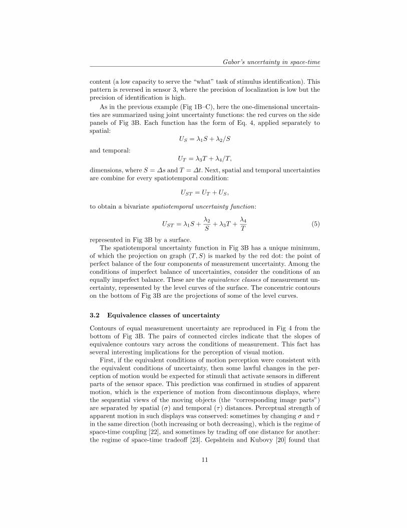
Now consider a more complex case where signals vary on two dimensions: spaceand time. Here, the measurement uncertainty has four components, illustratedin Fig 3A. The bottom of Fig 3A is a graph of the spatial and temporal sensorsizes (T, S) = (∆t,∆s). Every point in this graph corresponds to a “conditionof measurement” associated with the four properties of sensors.6 By Gabor’suncertainty relation, spatial and temporal intervals (∆t,∆s) are associated with,respectively, the spatial and temporal frequency intervals (∆ft, ∆fs).

The four-fold dependency is explained on the side panels of the figure usingGabor’s logons, each associated with a sensor labeled by a numbered disc. Forexample, in sensor 7 the spatial and temporal intervals are small, indicatinga good precision of spatial and temporal localization (i.e., concerning “where”and “when” the stimuli occurs). But the spatial and temporal frequency intervalsare large, indicating a low precision in measuring spatial and temporal frequency

6 Here the sensors are characterized by intervals following the standard notion thatbiological motion sensors are maximally activated when the stimulus travels somedistance ∆s over some temporal interval ∆t [17].

10

Gabor’s uncertainty in space-time

content (a low capacity to serve the “what” task of stimulus identification). Thispattern is reversed in sensor 3, where the precision of localization is low but theprecision of identification is high.

As in the previous example (Fig 1B–C), here the one-dimensional uncertain-ties are summarized using joint uncertainty functions: the red curves on the sidepanels of Fig 3B. Each function has the form of Eq. 4, applied separately tospatial:

US = λ1S + λ2/S

and temporal:UT = λ3T + λ4/T,

dimensions, where S = ∆s and T = ∆t. Next, spatial and temporal uncertaintiesare combine for every spatiotemporal condition:

UST = UT + US ,

to obtain a bivariate spatiotemporal uncertainty function:

UST = λ1S +λ2S

+ λ3T +λ4T

(5)

represented in Fig 3B by a surface.The spatiotemporal uncertainty function in Fig 3B has a unique minimum,

of which the projection on graph (T, S) is marked by the red dot: the point ofperfect balance of the four components of measurement uncertainty. Among theconditions of imperfect balance of uncertainties, consider the conditions of anequally imperfect balance. These are the equivalence classes of measurement un-certainty, represented by the level curves of the surface. The concentric contourson the bottom of Fig 3B are the projections of some of the level curves.

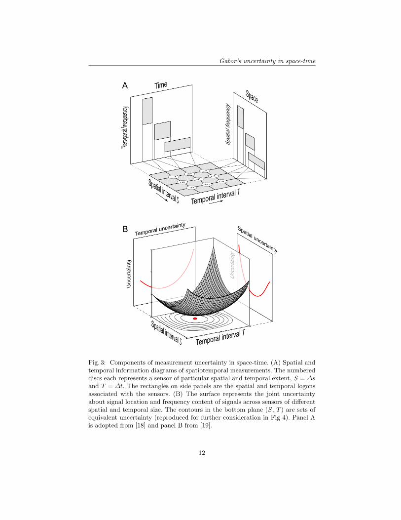
3.2 Equivalence classes of uncertainty

Contours of equal measurement uncertainty are reproduced in Fig 4 from thebottom of Fig 3B. The pairs of connected circles indicate that the slopes ofequivalence contours vary across the conditions of measurement. This fact hasseveral interesting implications for the perception of visual motion.

First, if the equivalent conditions of motion perception were consistent withthe equivalent conditions of uncertainty, then some lawful changes in the per-ception of motion would be expected for stimuli that activate sensors in differentparts of the sensor space. This prediction was confirmed in studies of apparentmotion, which is the experience of motion from discontinuous displays, wherethe sequential views of the moving objects (the “corresponding image parts”)are separated by spatial (σ) and temporal (τ) distances. Perceptual strength ofapparent motion in such displays was conserved: sometimes by changing σ and τin the same direction (both increasing or both decreasing), which is the regime ofspace-time coupling [22], and sometimes by trading off one distance for another:the regime of space-time tradeoff [23]. Gepshtein and Kubovy [20] found that

11

Gabor’s uncertainty in space-time

Fig. 3: Components of measurement uncertainty in space-time. (A) Spatial andtemporal information diagrams of spatiotemporal measurements. The numbereddiscs each represents a sensor of particular spatial and temporal extent, S = ∆sand T = ∆t. The rectangles on side panels are the spatial and temporal logonsassociated with the sensors. (B) The surface represents the joint uncertaintyabout signal location and frequency content of signals across sensors of differentspatial and temporal size. The contours in the bottom plane (S, T ) are sets ofequivalent uncertainty (reproduced for further consideration in Fig 4). Panel Ais adopted from [18] and panel B from [19].

12

Gabor’s uncertainty in space-time

Fig. 4: Equivalence classes of un-certainty. The contours representequal measurement uncertainty (re-produced from the bottom panelof Fig 3B) and the red circle rep-resents the minimum of uncertainty.The pairs of connected circles labeled“space-time coupling” and “space-time tradeoff” indicate why somestudies of apparent motion discovereddifferent regimes of motion perceptionin different stimuli [20, 21].

the two regimes of apparent motion were special cases of a lawful pattern: oneregime yielded to another as a function of speed, consistent with the predictionsillustrated in Fig 4.

Second, the regime of space-time coupling undermines one of the cornerstonesof the literature on visual perceptual organization: the proximity principle ofperceptual grouping [24, 25]. The principle is an experimental observations fromthe early days of the Gestalt movement, capturing the common observationthat the strength of grouping between image parts depends on their distance:the shorter the distance the stronger the grouping. In space-time, the principlewould hold if the strength of grouping had not changed, when increasing onedistance (σ or τ) was accompanied by decreasing the other distance (τ or σ):the regime of tradeoff [26]. The fact that the strength of grouping is maintainedby increasing both σ and τ , or by or decreasing both σ and τ , is inconsistentwith the proximity principle [21].

3.3 Spatiotemporal interaction: speed

Now let us consider the interaction of the spatial and temporal dimensions ofmeasurement. A key aspect of this interaction is the speed of stimulus variation:the rate of temporal change of stimulus intensity across spatial location. Thedimension of speed has been playing a central role in the theoretical and empiricalstudies of visual perception [27, 17, 28]. Not only is the perception of speed crucialfor the survival of mobile animals, but it also constitutes a rich source of auxiliaryinformation for parsing the optical stimulation [29, 30].

What is more, speed appears to play the role of a control parameter in theorganization of visual sensitivity. The shape of a large-scale characteristic ofvisual sensitivity (measured using continuous stimuli) is invariant with respectto speed [31, 32]. And a characteristic of the strength of perceived motion indiscontinuous stimuli (giving rise to “apparent motion”) collapse onto a singlefunction when plotted against speed [20].

13

Gabor’s uncertainty in space-time

Fig. 5: Economic measurement of speed. (A) The rectangle represents a sensordefined by spatial and temporal intervals (S and T ). From considerations ofparsimony, the sensor is more suitable for measurement of speed v2 = S/Tthan v1 or v3 since no part of S or T is wasted in measurement of v2. (B) Liebig’sbarrel. The shortest stave determines barrel’s capacity. Parts of longer staves arewasted since they do not affect the capacity.

From the present normative perspective, the considerations of speed measure-ment (combined with the foregoing considerations of measuring the location andfrequency content) of visual stimuli have two pervasive consequences, which arereviewed in some detail next. First, in a system optimized for the measurementof speed, the expected distribution of the quality of measurement has an invari-ant shape, distinct from the shape of such a distribution conceived before onehas taken into account the measurement of speed (Fig 4). Second, the dynamicsof visual measurement, and not only its static organization, will depend on themanner of interaction of the spatial and temporal aspects of measurement.

In Figs 3-4, a distribution of the expected uncertainty of measurement wasderived from a local constraint on measurement. The local constraint was definedseparately for the spatial and temporal intervals of the sensor. The considera-tions of speed measurement add another constraint, which has to do with therelationship between the spatial and temporal intervals.

The ability to measure speed by a sensor defined by spatial and temporalintervals depends on the extent of these intervals. As it is shown in Fig 5A,different ratios of the spatial extent to the temporal extent make the sensordifferently suitable for measuring different magnitudes of speed.

This argument is one consequence of the Law of The Minimum [33], illus-trated in Fig 5B using Liebig’s barrel. A broken barrel with the staves of differentlengths can hold as much content as the shortest stave allows. Using the stavesof different lengths is wasteful because a barrel with all staves as short as theshortest stave would do just as well. In other words, the barrel’s capacity islimited by the shortest stave.

Similarly, a sensor’s capacity for measuring the speed is limited by the extentof its spatial and temporal intervals. The capacity is not used fully if the spatialand temporal projections of vector v are larger or smaller than the spatial and

14

Gabor’s uncertainty in space-time

temporal extents allow (v1 and v3 in Fig 5B). Just as the extra length of thelong staves is wasted in the Liebig’s barrel, the spatial extent of the sensor iswasted in measurement of v1 and the temporal extent is wasted in measurementof v3. Let us therefore start with the assumption that the sensor defined by theintervals S and T is best suited for measuring speed v = S/T .

4 Optimal conditions for motion measurement

4.1 Minima of uncertainty

The optimal conditions of measurement are expected where the measurementuncertainty is the lowest. Using a shorthand notation for the spatial and temporalpartial derivatives of UST in Eq. 4, ∂US = ∂UST /∂S and ∂UT = ∂UST /∂T , theminimum of measurement uncertainty is the solution of

∂UT dT + ∂US dS = 0. (6)

The optimal condition for the entire space of sensors, disregarding individualspeeds, is marked as the red point in Fig 4. To find the minima for specificspeeds vi, let us rewrite Eq. 6 such that speed appears in the equation as anexplicit term. By dividing each side of Eq. 6 by dT , and using the fact thatv = dS/dT , it follows that

∂USvi + ∂UT = 0. (7)

The solution of Eq. 7 is a set of optimal conditions of measurement acrossspeeds. To illustrate the solution graphically, consider the vector form of Eq. 7,i.e., the scalar product ⟨

g(T,S), v(T,S)

⟩= 0, (8)

where the first term is the gradient of measurement uncertainty function,

g(T,S) = (∂uT , ∂uS), (9)

and the second term is the speed,

v(T,S) = (T, vT ), (10)

for sensors with parameters (T, S). For now, assume that the speed to which asensor is tuned is the ratio of spatial to temporal intervals (v = S/T ) that definethe logon of the sensor. (Normative considerations of speed tuning are reviewedin section Spatiotemporal interaction: speed.)

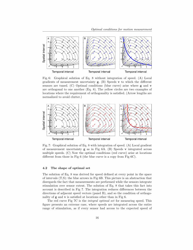
The two terms of Eq. 8 are shown in Fig 6: separately in panels A-B andtogether in panel C. The blue curve in panel C represents the set of conditionswhere vectors v and g are orthogonal to one another, satisfying Eq. 8. This curveis the optimal set for measuring speed while minimizing the uncertainty aboutsignal location and content.

15

Optimal conditions for motion measurement

Fig. 6: Graphical solution of Eq. 8 without integration of speed. (A) Localgradients of measurement uncertainty g. (B) Speeds v to which the differentsensors are tuned. (C) Optimal conditions (blue curve) arise where g and vare orthogonal to one another (Eq. 8). The yellow circles are two examples oflocations where the requirement of orthogonality is satisfied. (Arrow lengths arenormalized to avoid clutter.)

Fig. 7: Graphical solution of Eq. 8 with integration of speed. (A) Local gradientof measurement uncertainty g as in Fig 6A. (B) Speeds v integrated acrossmultiple speeds. (C) Now the optimal conditions (red curve) arise at locationsdifferent from those in Fig 6 (the blue curve is a copy from Fig 6C).

4.2 The shape of optimal set

The solution of Eq. 8 was derived for speed defined at every point in the spaceof intervals (T,S): the blue arrows in Fig 6B. This picture is an abstraction thatdisregards the fact that measurements are performed while the sensors integratestimulation over sensor extent. The solution of Eq. 8 that takes this fact intoaccount is described in Fig 7. The integration reduces differences between thedirections of adjacent speed vectors (panel B), and so the condition of orthogo-nality of g and v is satisfied at locations other than in Fig 6.

The red curve Fig 7C is the integral optimal set for measuring speed. Thisfigure presents an extreme case, where speeds are integrated across the entirerange of stimulation, as if every sensor had access to the expected speed of

16

Optimal conditions for motion measurement

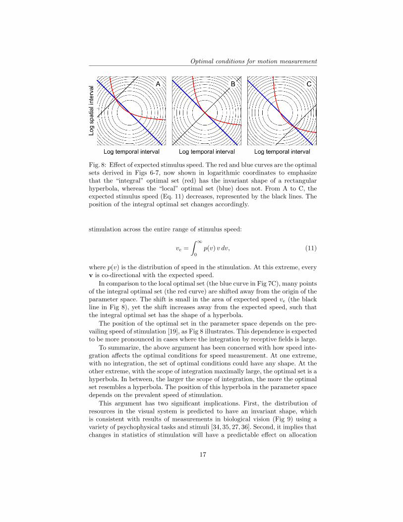
Fig. 8: Effect of expected stimulus speed. The red and blue curves are the optimalsets derived in Figs 6-7, now shown in logarithmic coordinates to emphasizethat the “integral” optimal set (red) has the invariant shape of a rectangularhyperbola, whereas the “local” optimal set (blue) does not. From A to C, theexpected stimulus speed (Eq. 11) decreases, represented by the black lines. Theposition of the integral optimal set changes accordingly.

stimulation across the entire range of stimulus speed:

ve =

∫ ∞0

p(v) v dv, (11)

where p(v) is the distribution of speed in the stimulation. At this extreme, everyv is co-directional with the expected speed.

In comparison to the local optimal set (the blue curve in Fig 7C), many pointsof the integral optimal set (the red curve) are shifted away from the origin of theparameter space. The shift is small in the area of expected speed ve (the blackline in Fig 8), yet the shift increases away from the expected speed, such thatthe integral optimal set has the shape of a hyperbola.

The position of the optimal set in the parameter space depends on the pre-vailing speed of stimulation [19], as Fig 8 illustrates. This dependence is expectedto be more pronounced in cases where the integration by receptive fields is large.

To summarize, the above argument has been concerned with how speed inte-gration affects the optimal conditions for speed measurement. At one extreme,with no integration, the set of optimal conditions could have any shape. At theother extreme, with the scope of integration maximally large, the optimal set is ahyperbola. In between, the larger the scope of integration, the more the optimalset resembles a hyperbola. The position of this hyperbola in the parameter spacedepends on the prevalent speed of stimulation.

This argument has two significant implications. First, the distribution ofresources in the visual system is predicted to have an invariant shape, whichis consistent with results of measurements in biological vision (Fig 9) using avariety of psychophysical tasks and stimuli [34, 35, 27, 36]. Second, it implies thatchanges in statistics of stimulation will have a predictable effect on allocation

17

Optimal conditions for motion measurement

Fig. 9: Human spatiotemporal contrast sensitivity function, shown as a surfacein A and a contour plot in B. Conditions of maximal sensitivity across speedsform the thick curve labeled “max.” The maximal sensitivity set has the shapepredicted by the normative theory: the red curve in Fig 7. The mapping frommeasurement intervals to stimulus frequencies is explained in [27, 19]. Both pan-els are adopted from [31].

of resources, helping the systems adapt to the variable stimulation, a themedeveloped in the next section.

5 Sensor allocation

5.1 Adaptive allocation

Allocation of sensors is likely to depend on several factors that determine sensorusefulness, such as sensory tasks and properties of stimulation. For example,when the organism needs to identify rather than localize the stimulus, largesensors are more useful than small ones. Allocation of sensors by their usefulnessis therefore expected to shift, for example as shown in Fig 2C.

Such shifts of allocation are expected also because the environment is highlyvariable. To insure that sensors are not allocated to stimuli that are absent oruseless, biological systems must monitor their environment and the needs ofmeasurement. As the environment or needs change, the same stimuli becomemore or less useful. The system must be able to reallocate its resources: changeproperties of sensors such as to better measure useful stimuli.

Because of the large but limited pool of sensors at their disposal, real sensorysystems occupy the middle ground between extremes of sensor “wealth.” Suchsystems can afford some specialization but they cannot be wasteful. They aretherefore subject to Gabor’s uncertainty relation, but they can alleviate conse-quences of the uncertainty relation, selectively and to some extent, by allocating

18

Sensor allocation

Spatial frequency (cyc/deg)

10

1

50

0.5

5

1010.5 50.1

0.2

0.4

0.6

0.8

Spatial frequency (cyc/deg)

Norm

aliz

ed

sensitiv

ity

1010.5 50.1

Spatial frequency (cyc/deg)

-50

05

01

00

1010.5 50.1

10

1

50

0.5

5

Te

mp

ora

lfr

eq

ue

ncy

(cyc/s

ec)

Te

mp

ora

lfr

eq

ue

ncy

(cyc/s

ec)

Se

nsitiv

ity

ch

an

ge

(%)

BA C

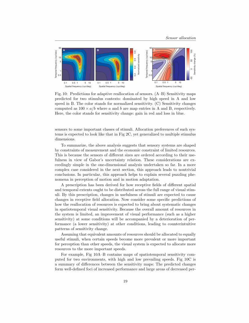
Fig. 10: Predictions for adaptive reallocation of sensors. (A–B) Sensitivity mapspredicted for two stimulus contexts: dominated by high speed in A and lowspeed in B. The color stands for normalized sensitivity. (C) Sensitivity changescomputed as 100× a/b where a and b are map entries in A and B, respectively.Here, the color stands for sensitivity change: gain in red and loss in blue.

sensors to some important classes of stimuli. Allocation preferences of such sys-tems is expected to look like that in Fig 2C, yet generalized to multiple stimulusdimensions.

To summarize, the above analysis suggests that sensory systems are shapedby constraints of measurement and the economic constraint of limited resources.This is because the sensors of different sizes are ordered according to their use-fulness in view of Gabor’s uncertainty relation. These considerations are ex-ceedingly simple in the one-dimensional analysis undertaken so far. In a morecomplex case considered in the next section, this approach leads to nontrivialconclusions. In particular, this approach helps to explain several puzzling phe-nomena in perception of motion and in motion adaptation.

A prescription has been derived for how receptive fields of different spatialand temporal extents ought to be distributed across the full range of visual stim-uli. By this prescription, changes in usefulness of stimuli are expected to causechanges in receptive field allocation. Now consider some specific predictions ofhow the reallocation of resources is expected to bring about systematic changesin spatiotemporal visual sensitivity. Because the overall amount of resources inthe system is limited, an improvement of visual performance (such as a highersensitivity) at some conditions will be accompanied by a deterioration of per-formance (a lower sensitivity) at other conditions, leading to counterintuitivepatterns of sensitivity change.

Assuming that equivalent amounts of resources should be allocated to equallyuseful stimuli, when certain speeds become more prevalent or more importantfor perception than other speeds, the visual system is expected to allocate moreresources to the more important speeds.

For example, Fig 10A–B contains maps of spatiotemporal sensitivity com-puted for two environments, with high and low prevailing speeds. Fig 10C isa summary of differences between the sensitivity maps: The predicted changesform well-defined foci of increased performance and large areas of decreased per-

19

Sensor allocation

formance. Gepshtein et al. [37] used intensive psychometric methods [38] to mea-sure the entire spatiotemporal contrast sensitivity function in different statistical“contexts” of stimulation. They found that sensitivity changes were consistentwith the predictions illustrated in Fig 10.

These results suggest a simple resolution to some long-standing puzzles inthe literature on motion adaptation. In early theories, adaptation was viewed asa manifestation of neural fatigue. Later theories were more pragmatic, assumingthat sensory adaptation is the organism’s attempt to adjust to the changingenvironment [39–42]. But evidence supporting this view has been scarce andinconsistent. For example, some studies showed that perceptual performanceimproved at the adapting conditions, but other studies reported the opposite[43, 44]. Even more surprising were systematic changes of performance for stimulivery different from the adapting ones [44]. According to the present analysis, suchlocal gains and losses of sensitivity are expected in a visual system that seeksto allocate its limited resources in face of uncertain and variable stimulation(Fig 10). Indeed, the pattern of gains and losses of sensitivity manifests anoptimal adaptive visual behavior.

This example illustrates that in a system with scarce resources optimizationof performance will lead to reduction of sensitivity to some stimuli. This phe-nomenon is not unique to sensory adaptation [45]. For example, demanding tasksmay cause impairment of visual performance for some stimuli, as a consequenceof task-driven reallocation of visual resources [46, 47].

5.2 Mechanism of adaptive allocation

From the above it follows that the shape of spatiotemporal sensitivity function,and also transformations of this function, can be understood by studying theuncertainties implicit to visual measurement. This idea received further supportfrom simulations of a visual system equipped with thousands of independent(uncoupled) sensors, each having a spatiotemporal receptive field [48, 49].

In these studies, spatiotemporal signals were sampled from known statisti-cal distributions. Receptive fields parameters were first distributed at random.They were then updated according to a generic rule of synaptic plasticity [50–53].Changes of receptive field amounted to small random steps in the parametersspace, modeled as stochastic fluctuations of the spatial and temporal extentsof receptive fields. Step length was proportional to the (local) uncertainty ofmeasurement by individual receptive fields. The steps were small where the un-certainty was low, and receptive fields changed little. Where the uncertainty washigh, the steps were larger, so the receptive fields tended to escape the high-uncertainty regions. The stochastic behavior led to a “drift” of receptive fieldsin the direction of low uncertainty of measurement [49], predicted by standardstochastic methods [54], as if the system sought stimuli that could be measuredreliably (cf. [55]).

Remarkably, the independent stochastic changes of receptive fields (their un-coupled “stochastic tuning”) steered the system toward the distribution of re-ceptive field parameters predicted by the normative theory, and forming the

20

Sensor allocation

distribution observed in human vision (Fig 9). When the distribution of stimulichanged, mimicking a change of sensory environment, the system was able tospontaneously discover an arrangement of sensors optimal for the new environ-ment, in agreement with the predictions illustrated in Fig 10 [56]. This is anexample of how efficient allocation of resources can emerge in sensory systemsby way of self-organization, enabling a highly adaptive sensory behavior in faceof the variable (and sometimes unpredictable) environment.

5.3 Conclusions

A study of allocation of limited resources for motion sensing across multiple spa-tial and temporal scales revealed that the optimal allocation entails a shape ofthe distribution of sensitivity similar to that found in human visual perception.The similarity suggested that several previously puzzling phenomena of visualsensitivity, adaptation, and perceptual organization have simple principled ex-planations. Experimental studies of human vision have confirmed the predictionsfor sensory adaptation. Since the optimal allocation is readily implemented inself-organizing neural networks by means of unsupervised leaning and stochasticoptimization, the present approach offers a framework for neuromorphic designof multiscale sensory systems capable of automated efficient tuning to the vary-ing optical environment.

Acknowledgments

This work was supported by the European Regional Development Fund, NationalInstitutes of Health Grant EY018613, and Office of Naval Research Multidisci-plinary University Initiative Grant N00014-10-1-0072.

21

References

References

1. Marr, D.: Vision: A computational investigation into the human representationand processing of visual information. W. H. Freeman, San Francisco (1982)

2. Gabor, D.: Theory of communication. Institution of Electrical Engineers 93 (PartIII) (1946) 429–457

3. Marcelja, S.: Mathematical description of the response by simple cortical cells.Journal of the Optical Society of America 70 (1980) 1297–1300

4. MacKay, D.M.: Strife over visual cortical function. Nature 289 (1981) 117–118

5. Daugman, J.G.: Uncertainty relation for the resolution in space spatial frequency,and orientation optimized by two-dimensional visual cortex filters. Journal of theOptical Society of America A 2(7) (1985) 1160–1169

6. Glezer, V.D., Gauzel’man, V.E., Iakovlev, V.V.: Principle of uncertainty in vision.Neirofiziologiia [Neurophysiology] 18(3) (1986) 307–312 PMID: 3736708.

7. Field, D.J.: Relations between the statistics of natural images and the responseproperties of cortical cells. J. Opt. Soc. Am. A 4 (1987) 2379–2394

8. Jones, A., Palmer, L.: An evaluation of the two-dimensional Gabor filter model ofsimple receptive fields in cat striate cortex. Journal of Neurophysiology 58 (1987)1233–1258

9. Simoncelli, E.P., Olshausen, B.: Natural image statistics and neural representation.Annual Review of Neuroscience 24 (2001) 1193–1216

10. Saremi, S., Sejnowski, T.J., Sharpee, T.O.: Double-Gabor filters are independentcomponents of small translation-invariant image patches. Neural Computation25(4) (2013) 922–939

11. Gabor, D.: Lectures on communication theory. Technical report 238 (1952) FallTerm, 1951.

12. Resnikoff, H.L.: The illusion of reality. Springer-Verlag New York, Inc., New York,NY, USA (1989)

13. MacLennan, B.: Gabor representations of spatiotemporal visual images. Technicalreport (1994) University of Tennessee, Knoxville, TN, USA.

14. Gepshtein, S., Tyukin, I.: Why do moving things look as they do? Vision. TheJournal of the Vision Society of Japan, Supp. 18 (2006) 64

15. von Neumann, J.: Zur Theorie der Gesellschaftsspiele. [On the theory of games ofstrategy]. Mathematische Annalen 100 (1928) 295–320 English translation in [57].

16. Luce, R.D., Raiffa, H.: Games and Decisions. John Wiley, New York (1957)

17. Watson, A.B., Ahumada, A.J.: Model of human visual-motion sensing. Journal ofthe Optical Society of America A 2(2) (1985) 322–341

18. Gepshtein, S.: Two psychologies of perception and the prospect of their synthesis.Philosophical Psychology 23 (2010) 217–281

19. Gepshtein, S., Tyukin, I., Kubovy, M.: The economics of motion perception andinvariants of visual sensitivity. Journal of Vision 7(8:8) (2007) 1–18

20. Gepshtein, S., Kubovy, M.: The lawful perception of apparent motion. Journal ofVision 7(8) (2007) 1–15 doi: 10.1167/7.8.9.

21. Gepshtein, S., Tyukin, I., Kubovy, M.: A failure of the proximity principle in theperception of motion. Humana Mente 17 (2011) 21–34

22. Korte, A.: Kinematoskopische Untersuchungen. Zeitschrift fur Psychologie 72(1915) 194–296

23. Burt, P., Sperling, G.: Time, distance, and feature tradeoffs in visual apparentmotion. Psychological Review 88 (1981) 171–195

22

References

24. Wertheimer, M.: Untersuchungen zur Lehre von der Gestalt, II. PsychologischeForschung 4 (1923) 301–350

25. Kubovy, M., Holcombe, A.O., Wagemans, J.: On the lawfulness of grouping byproximity. Cognitive Psychology 35 (1998) 71–98

26. Koffka, K.: Principles of Gestalt psychology. A Harbinger Book, Harcourt, Brace& World, Inc., New York, NY, USA (1935/1963)

27. Nakayama, K.: Biological image motion processing: A review. Vision Research25(5) (1985) 625–660

28. Weiss, Y., Simoncelli, E.P., Adelson, E.H.: Motion illusions as optimal percepts.Nature Neuroscience 5(6) (2002) 598–604

29. Longuet-Higgins, H.C., Prazdny, K.: The interpretation of a moving retinal image.Proceedings of the Royal Society of London. Series B, Biological Sciences 208(1173)(1981) 385–397

30. Landy, M., Maloney, L., Johnsten, E., Young, M.: Measurement and modelingof depth cue combinations: in defense of weak fusion. Vision Research 35 (1995)389–412

31. Kelly, D.H.: Motion and vision II. Stabilized spatio-temporal threshold surface.Journal of the Optical Society of America 69(10) (1979) 1340–1349

32. Kelly, D.H.: Eye movements and contrast sensitivity. In Kelly, D.H., ed.: VisualScience and Engineering. (Models and Applications). Marcel Dekker, Inc., NewYork, USA (1994) 93–114

33. Gorban, A., Pokidysheva, L., Smirnova, E., Tyukina, T.: Law of the minimumparadoxes. Bull Math Biol 73(9) (2011) 2013–2044

34. van Doorn, A.J., Koenderink, J.J.: Temporal properties of the visual detectabilityof moving spatial white noise. Experimental Brain Research 45 (1982) 179–188

35. van Doorn, A.J., Koenderink, J.J.: Spatial properties of the visual detectability ofmoving spatial white noise. Experimental Brain Research 45 (1982) 189–195

36. Laddis, P., Lesmes, L.A., Gepshtein, S., Albright, T.D.: Efficient measurement ofspatiotemporal contrast sensitivity in human and monkey. In: 41st Annual Meetingof the Society for Neuroscience. (Nov 2011) [577.20].

37. Gepshtein, S., Lesmes, L.A., Albright, T.D.: Sensory adaptation as optimal re-source allocation. Proceedings of the National Academy of Sciences, USA 110(11)(2013) 4368–4373

38. Lesmes, L.A., Gepshtein, S., Lu, Z.L., Albright, T.: Rapid estimation of thespatiotemporal contrast sensitivity surface. Journal of Vision 9(8) (2009) 696http://journalofvision.org/9/8/696/.

39. Sakitt, B., Barlow, H.B.: A model for the economical encoding of the visual imagein cerebral cortex. Biological Cybernetics 43 (1982) 97–108

40. Laughlin, S.B.: The role of sensory adaptation in the retina. Journal of Experi-mental Biology 146(1) (1989) 39–62

41. Wainwright, M.J.: Visual adaptation as optimal information transmission. VisionResearch 39 (1999) 3960–3974

42. Laughlin, S.B., Sejnowski, T.J.: Communication in Neuronal Networks. Science301(5641) (2003) 1870–1874

43. Clifford, C.W.G., Wenderoth, P.: Adaptation to temporal modulation can enhancedifferential speed sensitivity. Vision Research 39 (1999) 4324–4332

44. Krekelberg, B., Van Wezel, R.J., Albright, T.D.: Adaptation in macaque MTreduces perceived speed and improves speed discrimination. Journal of Neuro-physiology 95 (2006) 255–270

45. Gepshtein, S.: Closing the gap between ideal and real behavior: scientific vs. engi-neering approaches to normativity. Philosophical Psychology 22 (2009) 61–75

23

References

46. Yeshurun, Y., Carrasco, M.: Attention improves or impairs visual performance byenhancing spatial resolution. Nature 396 (1998) 72–75

47. Yeshurun, Y., Carrasco, M.: The locus of attentional effects in texture segmenta-tion. Nature Neuroscience 3(6) (2000) 622–627

48. Jurica, P., Gepshtein, S., Tyukin, I., Prokhorov, D., van Leeuwen, C.: Unsupervisedadaptive optimization of motion-sensitive systems guided by measurement uncer-tainty. In: International Conference on Intelligent Sensors, Sensor Networks andInformation, ISSNIP 2007. 3rd, Melbourne, Qld (2007) 179–184 doi: 10.1109/ISS-NIP.2007.4496840.

49. Jurica, P., Gepshtein, S., Tyukin, I., van Leeuwen, C.: Sensory optimiza-tion by stochastic tuning. Psychological Review 120(4) (2013) 798–816 doi:10.1037/a0034192.

50. Hebb, D.O.: The Organization of Behavior. John Wiley, New York (1949)51. Bienenstock, E.L., Cooper, L.N., Munro, P.W.: Theory for the development of

neuron selectivity: orientation specificity and binocular interaction in visual cortex.Journal of Neuroscience 2 (1982) 32–48

52. Paulsen, O., Sejnowski, T.J.: Natural patterns of activity and long-term synapticplasticity. Current Opinion in Neurobiology 10(2) (2000) 172–180

53. Bi, G., Poo, M.: Synaptic modification by correlated activity: Hebb’s postulaterevisited. Annual Review of Neuroscience 24 (2001) 139–166

54. Gardiner, C.W.: Handbook of Stochastic Methods: For Physics, Chemistry andthe Natural Sciences. Springer, New York (1996)

55. Vergassola, M., Villermaux, E., Shraiman, B.I.: ‘Infotaxis’ as a strategy for search-ing without gradients. Nature 445 (2007) 406–409

56. Gepshtein, S., Jurica, P., Tyukin, I., van Leeuwen, C., Albright, T.D.: Optimal sen-sory adaptation without prior representation of the environment. In: 40th AnnualMeeting of the Society for Neuroscience. (Nov 2010) [731.7].

57. Taub, A.H., ed.: John von Neumann: Collected Works. Volume VI: Theory ofGames, Astrophysics, Hydrodynamics and Meteorology. Pergamon Press, NewYork, NY, USA (1963)

58. Shannon, C.E.: A mathematical theory of communication. Bell System TechnicalJournal 27 (1948) 379–423, 623–656

59. Jaynes, E.T.: Information theory and statistical mechanics. Physical Review 106(1957) 620–630

60. Gorban, A.: Maxallent: Maximizers of all entropies and uncertainty of uncertainty.Computers and Mathematics with Applications 65(10) (2013) 1438–1456

61. Cover, T.M., Thomas, J.A.: Elements of Information Theory. John Wiley, NewYork (2006)

24

Appendices

6 Appendices

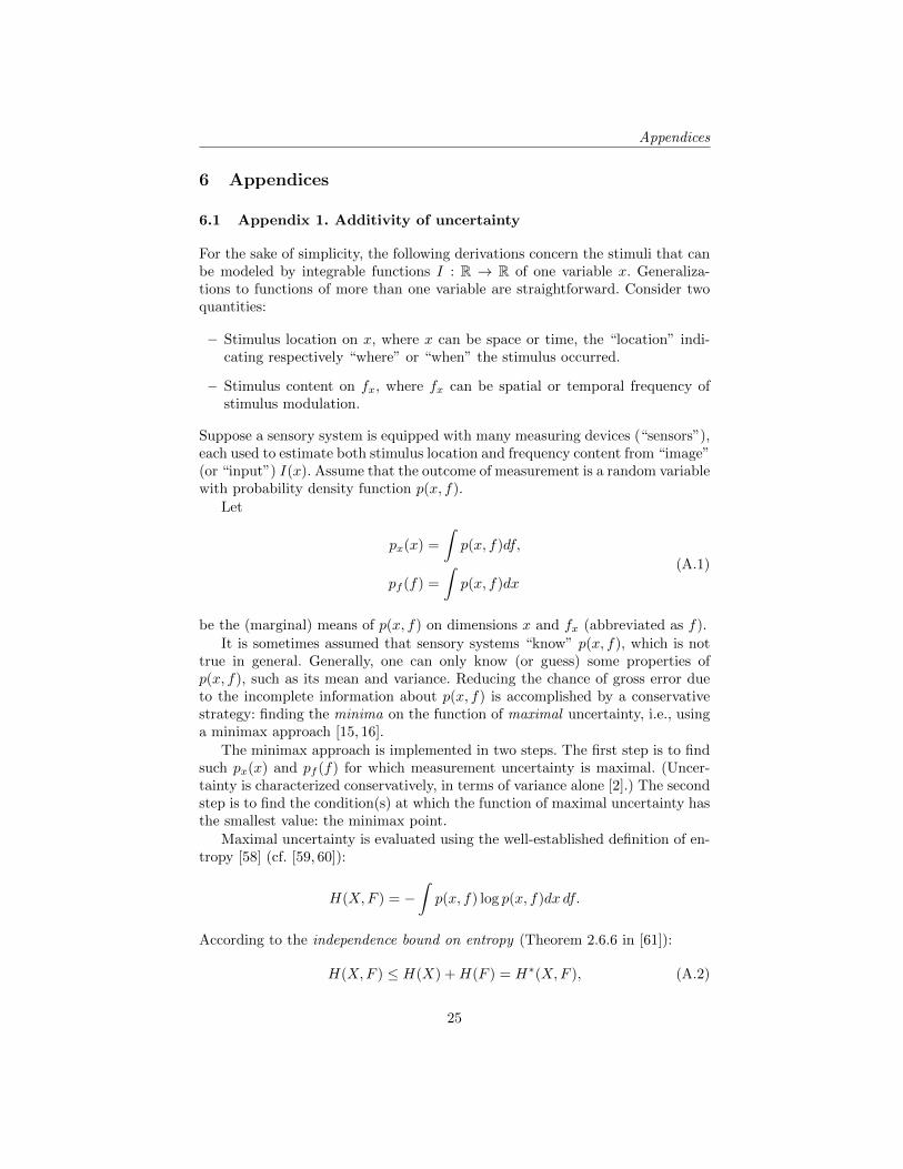
6.1 Appendix 1. Additivity of uncertainty

For the sake of simplicity, the following derivations concern the stimuli that canbe modeled by integrable functions I : R → R of one variable x. Generaliza-tions to functions of more than one variable are straightforward. Consider twoquantities:

– Stimulus location on x, where x can be space or time, the “location” indi-cating respectively “where” or “when” the stimulus occurred.

– Stimulus content on fx, where fx can be spatial or temporal frequency ofstimulus modulation.

Suppose a sensory system is equipped with many measuring devices (“sensors”),each used to estimate both stimulus location and frequency content from “image”(or “input”) I(x). Assume that the outcome of measurement is a random variablewith probability density function p(x, f).

Let

px(x) =

∫p(x, f)df,

pf (f) =

∫p(x, f)dx

(A.1)

be the (marginal) means of p(x, f) on dimensions x and fx (abbreviated as f).

It is sometimes assumed that sensory systems “know” p(x, f), which is nottrue in general. Generally, one can only know (or guess) some properties ofp(x, f), such as its mean and variance. Reducing the chance of gross error dueto the incomplete information about p(x, f) is accomplished by a conservativestrategy: finding the minima on the function of maximal uncertainty, i.e., usinga minimax approach [15, 16].

The minimax approach is implemented in two steps. The first step is to findsuch px(x) and pf (f) for which measurement uncertainty is maximal. (Uncer-tainty is characterized conservatively, in terms of variance alone [2].) The secondstep is to find the condition(s) at which the function of maximal uncertainty hasthe smallest value: the minimax point.

Maximal uncertainty is evaluated using the well-established definition of en-tropy [58] (cf. [59, 60]):

H(X,F ) = −∫p(x, f) log p(x, f)dx df.

According to the independence bound on entropy (Theorem 2.6.6 in [61]):

H(X,F ) ≤ H(X) +H(F ) = H∗(X,F ), (A.2)

25

Appendices

where

H(X) =−∫px(x) log px(x)dx,

H(F ) =−∫pf (f) log pf (f)df.

Therefore, the uncertainty of measurement cannot exceed

H∗(X,F ) =−∫px(x) log px(x)dx

−∫pf (f) log pf (f)df.

(A.3)

Eq. A.3 is the “envelope” of maximal measurement uncertainty: a “worst-case”estimate.

By the Boltzmann theorem on maximum-entropy probability distributions[61], the maximal entropy of probability densities with fixed means and variancesis attained when the functions are Gaussian. Then, maximal entropy is a sumof their variances [61] and

px(x) =1

σx√

2πe−x

2/2σ2x ,

pf (f) =1

σf√

2πe−f

2/2σ2f ,

where σx and σf are the standard deviations. Then maximal entropy is

H = σ2x + σ2

f . (A.4)

That is, when p(x, f) is unknown, and all one knows about marginal distribu-tions px(x) and pf (f) is their means and variances, the maximal uncertainty ofmeasurement is the sum of variances of the estimates of x and f . The follow-ing minimax step is to find the conditions of measurement at which the sum ofvariances is the smallest.

6.2 Appendix 2. Improving resolution by multiple sampling

How does an increased allocation of resources to a specific condition of measure-ment improve resolution (spatial or temporal) at that condition? Consider set Ψof sampling functions

ψ(sσ + δ), σ ∈ R, σ > 0, δ ∈ R,

where σ is a scaling parameter and δ is a translation parameter. For a broad classof functions ψ(·), any element of Ψ can be obtained by addition of weighted andshifted ψ(s). The following argument proves that any function from a sufficiently

26

Appendices

broad class that includes ψ(sσ + δ) can be represented by a weighted sum oftranslated replicas of ψ(s).

Let ψ∗(s) be a continuous function that can be expressed as a sum of aconverging series of harmonic functions:

ψ∗(s) =∑i

ai cos(ωis) + bi sin(ωis).

For example, Gaussian sampling functions of arbitrary widths can be expressedas a sum of cos(·) and sin(·). Let us show that, if |ψ(s)| is Riemann-integrable,i.e., if

−∞ <

∫ ∞−∞|ψ(s)|ds <∞,

and its Fourier transform, ψ, does not vanish for all ω ∈ R: ψ(ω) 6= 0 (i.e., itsspectrum has no “holes”), then the following expansion of ψ∗ is possible

ψ∗(s) =∑i

ciψ(s+ di) + ε(s), (A.5)

where ε(s) is a residual that can be arbitrarily small. This goal is attained byproving identities

cos(ω0s) =∑i

ci,1ψ(s+ di,1) + ε1(s),

sin(ω0s) =∑i

ci,2ψ(s+ di,2) + ε2(s),(A.6)

where ci,1, ci,2 and di,1, di,2 are real numbers, while ε1(s) and ε2(s) are arbitrarilysmall residuals.

First, write the Fourier transform of ψ(s) as

ψ(ω) =

∫ ∞−∞

ψ(s)e−iωsds,

and multiply both sides of the above expression by eiω0υ:

eiω0υψ(ω) = eiω0υ

∫ ∞−∞

ψ(s)e−iωsds =

∫ ∞−∞

ψ(s)e−i(ωs−ω0υ)ds. (A.7)

Change the integration variable:

x = ωs− ω0υ ⇒ dx = ωds, s =x+ ω0υ

ω,

such that Eq. A.7 transforms into

eiω0υψ(ω) =1

ω

∫ ∞−∞

ψ

(x+ ω0υ

ω

)e−ixdx.

27

Appendices

Notice that ψ(ω) = a(ω) + ib(ω). Hence

eiω0υψ(ω) = eiω0υ(a(ω) + ib(ω)) = (cos(ω0υ) + i sin(ω0υ))(a(ω) + ib(ω))

and

eiω0υψ(ω) = (cos(ω0υ)a(ω)− sin(ω0υ)b(ω)) + i(cos(ω0υ)b(ω) + sin(ω0υ)a(ω)).

Since ψ(ω) 6= 0 is assumed for all ω ∈ R, then a(ω) + ib(ω) 6= 0. In other words,either a(ω) 6= 0 or b(ω) 6= 0 should hold. For example, suppose that a(ω) 6= 0.Then

Re(eiω0υψ(ω)

)+b(ω)

a(ω)Im(eiω0υψ(ω)

)= cos(ω0υ)

(a2(ω) + b2(ω)

a(ω)

).

Therefore

cos(ω0υ) =

(a(ω)

a2(ω) + b2(ω)

)Re

(1

ω

∫ ∞−∞

ψ

(x+ ω0υ

ω

)e−ixdx

)+

(b(ω)

a2(ω) + b2(ω)

)Im

(1

ω

∫ ∞−∞

ψ

(x+ ω0υ

ω

)e−ixdx

).

(A.8)

Because function ψ(s) is Riemann-integrable, the integrals in Eq. A.8 can beapproximated as

Re

(1

ω

∫ ∞−∞

ψ

(x+ ω0υ

ω

)e−ixdx

)=∆

ω

N∑k=1

ψ

(xk + ω0υ

ω

)cos(xk) +

ε1(υ,N)

2ω,

(A.9)

Im

(1

ω

∫ ∞−∞

ψ

(x+ ω0υ

ω

)e−ixdx

)=∆

ω

N∑p=1

ψ

(xp + ω0υ

ω

)sin(xp) +

ε1(υ,N)

2ω,

(A.10)where xk and xp are some elements of R. To complete the proof, denote

c2i,1 =∆

ω

a(ω)

a2(ω) + b2(ω)cos(xi), c2i−1,1 =

∆

ω

a(ω)

a2(ω) + b2(ω)sin(xi),

d2i,1 = d2i−1,1 =xiω.

From Eqs. A.8–A.10 it follows that

cos(ω0υ) =

2N∑j=1

cj,1ψ(ω0υ

ω+ dj,1

)+ ε1(υ,N).

Given that ψ(ω) 6= 0 for all ω, and letting ω = ω0, it follows that

cos(ω0υ) =

2N∑j=1

cj,1ψ (υ + dj,1) + ε1(υ,N), (A.11)

28

Appendices

where

ε1(υ,N) = ε1(υ,N)a(ω0)

2ω0(a2(ω0) + b2(ω0)). (A.12)

An analogue of Eq. A.11 for sin(ω0υ) follows from sin(ω0υ) = cos(ω0υ + π/2).This completes the proof of Eq. A.6 and hence of Eq. A.5.

29