Sampling-based Algorithms for Optimal Motion PlanningUsing Closed-loop Prediction

Oktay Arslan1 Karl Berntorp2 Panagiotis Tsiotras3

Abstract— Motion planning under differential constraints,kinodynamic motion planning, is one of the canonical problemsin robotics. Currently, state-of-the-art methods evolve aroundkinodynamic variants of popular sampling-based algorithms,such as Rapidly-exploring Random Trees (RRTs). However,there are still challenges remaining, for example, how to includecomplex dynamics while guaranteeing optimality. If the open-loop dynamics are unstable, exploration by random sampling incontrol space becomes inefficient. We describe a new sampling-based algorithm, called CL-RRT#, which leverages ideas fromthe RRT# algorithm and a variant of the RRT algorithm thatgenerates trajectories using closed-loop prediction. The ideaof planning with closed-loop prediction allows us to handlecomplex unstable dynamics and avoids the need to find com-putationally hard steering procedures. The search techniquepresented in the RRT# algorithm allows us to improve thesolution quality by searching over alternative reference tra-jectories. Numerical simulations using a nonholonomic systemdemonstrate the benefits of the proposed approach.

I. INTRODUCTION

Motion planning is ubiquitous in many applications wheredifferent levels of autonomy is desired. Loosely speaking,given a system that is subject to a set of differential con-straints, an initial state, a final state, a set of obstacles, and agoal region, the motion-planning problem is to find a controlinput that drives the system from its initial state to the goalregion. This problem is computationally hard to solve [15].

One approach to solve the motion-planning problems isto divide the problem into two subproblems: path planningand path tracking. The main drawback of this approach islack of dynamic feasibility guarantees. Still, it has beensuccessfully applied to robotic applications in which the un-derlying system has redundant control authority (e.g., roboticmanipulators). Another class of algorithms is randomizedplanners, which solve the motion-planning problem in asingle step. Notably, the kinodynamic version of Rapidly-Exploring Random Tree (RRT) incrementally grows a treeof trajectories in the state space by sampling control inputsand simulating the motion of the system with these randomcontrol inputs over a time horizon [12], [13]. Hence, thetrajectories that are generated by RRT are dynamically

1Oktay Arslan is a Robotics, PhD Candidate with the D. GuggenheimSchool of Aerospace Engineering and the Institute for Robotics and In-telligent Machines at the Georgia Institute of Technology, Atlanta, GA30332, USA, Email:oktay@gatech.edu. He performed this research whileat Mitsubishi Electric Research Laboratories, Cambridge, MA 02139, USA.

2Karl Berntorp is with Mitsubishi Electric Research Laboratories, Cam-bridge, MA 02139, USA, Email:karl.o.berntorp@ieee.org.

3Panagiotis Tsiotras is with the faculty of D. Guggenheim Schoolof Aerospace Engineering and the Institute for Robotics and IntelligentMachines at the Georgia Institute of Technology, Atlanta, GA 30332-0150,USA, Email: tsiotras@gatech.edu.

feasible by construction. Recently, RRT and its variantswere successfully applied to robotic systems [10], [14] anddifferent classes of stochastic problems [2]. Unlike standardRRT, these variants were usually implemented to computea solution quickly and improve it in the remaining time untilthe execution of the motion plan. However, RRT computessuboptimal solutions [7].

One drawback with kinodynamic RRT is that explorationvia random selection of control inputs is inefficient whenthe dynamics are complex and/or unstable. To remedy this,[11] proposed CL-RRT, which uses closed-loop predictionfor trajectory generation. Instead of sampling in the controlspace, the proposed approach grows a tree in the referencespace. Each path of the tree represents a reference trajectorythat acts as an input to the closed-loop system. The desiredbehaviors of the system are prescribed as specifications fora controller that is used to track a given reference trajectory.Each edge of the tree is associated with a segment of areference trajectory and a state trajectory of the system,computed by closed-loop prediction.

Several papers address the suboptimality of RRT. In [7],an algorithm with asymptotic optimality guarantee, RRT∗,was developed. RRT∗ has been extended to solve motionplanning problems under differential constraints [6], [8].The proposed algorithms are asymptotically optimal whena steering procedure that satisfies certain conditions is pro-vided. However, developing efficient steering procedures thatsolve point-to-point motion planning, essentially a two-pointboundary value problem, is generally hard [16].

Here, we propose a new asymptotically optimal motion-planning algorithm, CL-RRT#, by leveraging ideas fromthe CL-RRT [11] and the RRT# algorithms [3]–[5]. Tohandle differential constraints, instead of sampling in thecontrol space, our approach samples in the output spaceand incrementally grows a graph whose edges correspondto segments of reference trajectories. The algorithm alsokeeps another graph to store state trajectories of the closed-loop system when it is inputed with a certain path inthe graph of reference trajectories. Hence, we avoid theneed for complicated steering procedures and the resultingtrajectory satisfies the differential constraints by construction.To improve the solution quality, CL-RRT# searches amongalternative paths of the graph of reference trajectories. Theproposed algorithm checks different reference trajectoriesand simulates the system forward in time, as needed. Finally,the algorithm provides the segments of reference trajectoriesthat yield the lowest-cost state trajectory of the closed-loopsystem.

arX

iv:1

601.

0632

6v1

[cs

.RO

] 2

3 Ja

n 20

16

II. PROBLEM FORMULATION

Let X ⊆ Rn, Y ⊆ Rp and U ⊆ Rm be compact sets.We assume that the system dynamics can be described by anonlinear differential equation of the form

x(t) =f(x(t), u(t)), x(0) = x0,

y(t) =h(x(t), u(t)), (1)

where the system state x(t) ∈ X , the system output y(t) ∈Y , the control u(t) ∈ U , for all t, x0 ∈ X , and f and h aresmooth (continuously differentiable) functions describing thetime evolution of the system dynamics. Let X denote the setof all essentially bounded measurable functions mapped from[0, T ] to X for any T ∈ R>0 and define Y and U similarly.The functions in X , Y , and U are called state trajectories,output trajectories, and controls, respectively.

Let Xobs and Xgoal, called the obstacle space and the goalregion, be open subsets of X . Let Xfree, also called the freespace, denote the set defined as X \Xobs.

The smooth function h describes the output y that we wishto control. Loosely speaking, we are particularly interestedin the class of control problems in which we wish to track atime-varying reference trajectory r(t). called the trajectory-generation problem. We assume that given a desired outputvalue y′ ∈ Y , and a current output value y ∈ Y of thesystem, the control law φ : (y′, y) 7→ u ∈ U computesa control input such that the closed-loop simulation of thesystem yields a good tracking performance as time evolves.

A. Problem Statement

Given the state space X , obstacle region Xobs, goal regionXgoal, and smooth functions f and h that describe the systemdynamics, find a reference trajectory r ∈ Y with domain[0, T ] for some T ∈ R>0 such that the corresponding uniquestate trajectory x ∈ X , output trajectory y ∈ Y , and controlu ∈ U that are computed by closed-loop simulation,• obeys the differential constraints,

x(t) = f(x(t), u(t)) x(0) = x0,

y(t) = h(x(t), u(t)) for all t ∈ [0, T ],

• avoids the obstacles, i.e., x(t) ∈ Xfree for all t ∈ [0, T ],• reaches the goal region, i.e., x(T ) ∈ Xgoal,• and minimizes J(x, u, r) =

∫ T0g(x(t), u(t), r(t)) dt

B. Primitive Procedures

Following are the definitions of the primitive proceduresused by the CL-RRT# algorithm (for details, see [7]).

Sampling: Sample : ω 7→ {Samplei(ω)}i∈N0⊂ Yfree re-

turns independent and identically distributed (i.i.d.) samplesSamplei, i ∈ N0 from Yfree.

Nearest Neighbor: Given a graph Gy = (Vy, Ey), whereVy ∈ Y , a point y ∈ Y , the function Nearest : (Gy, y) 7→vy ∈ Vy returns the node in Vy that is “closest” to y in termsof a given distance function. We use the Euclidean distance.

Near Neighbors: Given a graph Gy = (Vy, Ey), whereVy ∈ Y , a point y ∈ Y , and a positive real number d ∈R>0, the function Nearest : (Gy, y, d) 7→ vy ∈ V ′y ⊂ Vy

returns the nodes in Vy that are contained in a ball of radiusd centered at y.

Steering: Given two points yfrom, yto ∈ Y , the functionSteer : (yfrom, yto) 7→ y′ returns a point y′ ∈ Y suchthat y′ is “closer” to yto than yfrom is. In this work, thepoint y′ returned by the function Steer will be such thaty′ minimizes ‖y′− yto‖ while at the same time maintaining‖y′ − yfrom‖ ≤ η, for a predefined η > 0.

Closed-loop Prediction: Given a state x ∈ Xfree, andan output trajectory σy ∈ Y , the function Propagate :(x, σy) 7→ σx ∈ X returns the state trajectory that iscomputed by simulating the system dynamics forward in timewith the initial state x, and the reference trajectory σy .

Collision Test: Given two points yfrom, yto ∈ Gy , theBoolean function ObstacleFree(yfrom, yto) returns True ifthe line segment between yfrom and yto lies in Yfree andFalse otherwise.

Cost-to-come Values: Given a graph Gy = (Vy, Ey), let g∗

denote the optimal cost-to-come value of the node vy ∈ Vythat can be achieved in Gy . Each node vy ∈ Vy is associatedwith two estimates of the optimal cost-to-come value (see [3],[9]). The g-value of vy is the cost of the path to vy froma given initial state yinit ∈ Yfree. The one step look-aheadg-value of vy is denoted with g and defined as

vy.g =

0, if vy.y = yinit,

miney∈Ey,pred

(vy,pred.g + Cost(σ)) , otherwise,

where Ey,pred = incoming(Gy, vy), vy,pred = ey.tail, andσ is the state trajectory that is computed via closed-loopprediction, i.e., the dynamical system is simulated forwardin time with the initial state vy,pred.pσ.back() and thereference trajectory ey.σ.

Heuristic Value: Given a node vy ∈ Vy , and an outputgoal region Ygoal, the function ComputeHeuristic :(vy, Ygoal) 7→ r returns an estimate r of the optimal costfrom vy to Ygoal; it return zero if vy ∈ Ygoal. In this paper,we always assume that ComputeHeuristic computes anadmissible heuristic, that is, it never overestimates the actualcost of reaching Ygoal.

Queue Operations: Nodes of the computed graphs areassociated with some keys and priority queues are used tosort these nodes based on the precedence relation betweenkeys. The following functions are implemented to maintaina given priority queue Q:• Q.top key() returns the highest priority of all nodes in

the priority queue Q with the smallest key value if thequeue is not empty. If Q is empty, then Q.top key()returns a key value of k = [∞;∞].

• Q.pop() deletes the node with the highest priority in thepriority queue Q and returns a reference to the node.

• Q.update(vy, k) sets the key value of the node vy tok and reorders the priority queue Q.

• Q.insert(vy, k) inserts the node vy into the priorityqueue Q with the key value k.

• Q.remove(vy) removes the node vy from the priorityqueue Q.

Initialization: Given an initial point xinit ∈ X , a goalregion in the output space Ygoal ⊂ Y , the functionInitialize : (xinit, Ygoal) 7→ (Gy,Gσ,Q,Qgoal) returnsa graph Gy that has only node vy , whose output point isvy.y = OutputMap(xinit), a graph Gσ that has the onlynode vσ , whose trajectory is a single point vσ.σ = xinit,and empty priority queues Q and Qgoal that are used forordering of nongoal and goal nodes, which represent pointsin Y , respectively.

Exploration: Given a tuple of data structures S =(Gy,Gσ,Q,Qgoal), where Gy and Gσ are graphs whose nodesrepresent points in Y and trajectories in X , respectively, andQ and Qgoal are priority queues that are used for orderingof nongoal and goal nodes that represent points in Y , a goalregion in the output space Ygoal ⊂ Y , and a point y ∈ Y , thefunction Extend : (S, Ygoal, y) 7→ S ′ = (G′y,G′σ,Q′,Q′goal)includes a new node, multiple edges to Gy and multiplenodes, edges to Gσ , updates the priorities of nodes in Qand Qgoal and returns an updated tuple S ′.

Exploitation: Given a tuple of data structures S =(Gy,Gσ,Q,Qgoal), where Gy and Gσ are graphs whose nodesrepresent points in Y and trajectories in X , respectively, andQ and Qgoal are priority queues that are used for orderingof nongoal and goal nodes that represent points in Y , thefunction Replan : S 7→ S ′ = (G′y,G′σ,Q′,Q′goal) rewires theparent node of the nodes in Gy based on their cost-to-comevalues, includes new nodes and edges in Gσ if necessary, thatis, propagating dynamics of the system for new sequence ofreference trajectories, and returns an updated tuple S ′.

Construction of Solution: Given a tuple of data structuresS = (Gy,Gσ,Q,Qgoal), the function ConstrSolution :S 7→ Tx returns a tree whose edges and nodes representsimulated trajectories in X and the corresponding internalstates of the nodes of Gy . These trajectories are computedby propagating the dynamics with reference trajectories thatare encoded in a tree of Gy , which is formed by the edgesbetween nodes of Gy and their parent nodes.

Graph and List Operations: The following functions areused in the CL-RRT# algorithm.• Given a node v ∈ V in a directed graph G =

(V,E), the set-valued function succ : (G, v) 7→V ′ ⊆ V returns the nodes in V that are the headsof the edges emanating from v, that is, succ(G, v) :={v′ ∈ V : e.tail = v and e.head = v′, e ∈ E} .

• Given a node v ∈ V in a directed graph G =(V,E), the set-valued function pred : (G, v) 7→V ′ ⊆ V returns the nodes in V that are the tailsof the edges going into v, that is, pred(G, v) :={v′ ∈ V : e.tail = v′ and e.head = v, e ∈ E} .

• Given a node v ∈ V in a directed graph G = (V,E),the set-valued function outgoing : (G, v) 7→ E′ ⊆E returns the edges in E whose tail is v, that is,outgoing(G, v) := {e ∈ E : e.tail = v} .

• Given a node v ∈ V in a directed graph G = (V,E),the set-valued function incoming : (G, v) 7→ E′ ⊆E returns the edges in E whose head is v, that is,incoming(G, v) := {e ∈ E : e.head = v} .

TABLE I: The node (OutNode) and edge (OutEdge) data structuresfor points and trajectories in output space, respectively

field type descriptiony vector ∈ Rp output point associated with this nodeg real ∈ R cost-to-come valueg real ∈ R one step look-ahead g-valueh real ∈ R heuristic value for the cost between y and

Ygoal

py OutNode reference to the parent output nodepσ TrajNode reference to the parent trajectory noder trajectory ∈ Y output trajectory associated with this edge

tail OutNode reference to the tail output nodehead OutNode reference to the head output node

• Given a list of nodes Vz , where its nodes representpoints in Z, and a point z ∈ Z, the function find :(Vz, z) 7→ vz ∈ Vz returns the node in Vz that satisfiesvz.z = z if there exists any such node, null otherwise.

• Given a list of nodes Vz , where its nodes representpoints in Z, the function back returns a reference to thelast node in the list if it is not empty, and null otherwise.

• Given a list of nodes Vz , where its nodes representpoints in Z, the function front returns a referenceto the first node in the list if it is not empty, and nullotherwise.

III. THE CL-RRT#ALGORITHM

A. Details of Data Structures

Each node vy in the graph Gy is an OutNode datastructure, summarized in Table I. Each node vy is associatedwith a reference point y ∈ Rm. It contains two estimates ofthe optimal cost-to-come value between the initial referencepoint and y, namely, cost-to-come value g and one step look-ahead g-value g. It also keeps a heuristic value h, which isan underestimate of the optimal cost value between y andYgoal, to guide and reduce the search effort. Whenever g isupdated during the replanning procedure, the reference nodethat yields the corresponding minimum cost-to-come valueis stored in the parent reference node py . Lastly, pσ is thetrajectory that is computed by closed-loop prediction whenthe system is simulated with the reference trajectory betweenthe nodes py and vy . Its terminal state represents the internalstate associated with vy .

Each edge ey in the graph Gy is an OutEdge datastructure, summarized in Table I. Each edge ey is associatedwith a trajectory r ∈ Y . It also contains two output nodes,namely, tail and head, which represent the tail and thehead output nodes of ey , respectively.

Each node vσ in the graph Gσ is a TrajNode datastructure, summarized in Table II. Each node vσ is associatedwith a trajectory σ ∈ X . It contains an output edge ey , whichcorresponds to the reference trajectory that yields σ as theclosed-loop prediction. It also keeps a list of outgoing outputedges outgoing, and this list is used to compute outgoingtrajectory nodes emanating from the terminal state of σ.

Each edge eσ in the graph Gσ is a TrajEdge datastructure, summarized in Table II. Each edge eσ is associatedwith a trajectory σ ∈ X . It contains two trajectory nodes,

TABLE II: The node (TrajNode) and edge (TrajEdge) data struc-tures for trajectories in state space

field type descriptionσ trajectory ∈ X state trajectory associated with this nodeey OutEdge reference to the output edge

outgoing OutEdge array list of outgoing output edgesσ trajectory ∈ X state trajectory associated with this edge

tail TrajNode reference to the tail trajectory nodehead TrajNode reference to the head trajectory node

namely, tail and head which represent the tail and the headtrajectory nodes of eσ , respectively.

B. Details of the Procedures

Algorithm 1 gives the body of the CL-RRT# algorithm.First, the algorithm initializes the tuple of data structures Sthat is incrementally grown and updated as exploration andexploitation are performed (Line 3). The tuple S contains thegraphs Gy and Gσ , which are used to store output nodes andstate trajectory nodes, respectively, and the priority queuesQ and Qgoal. The details of Initialize are given inAlgorithm 2. The graph Gσ is created with no edges andvσ as its only node. This node represents a state trajectorythat contains only the initial state xinit. Then, likewise, thegraph Gy is initialized with no edges and vy as its only nodethat represents yinit. The g- and g-values of vy are set withzero cost value. The parent trajectory node of vy is set withthe reference to the node vσ .

Algorithm 1: The CL-RRT# Algorithm1 CL-RRT#(xinit, Xgoal, X)2 Ygoal := OutputMap(Xgoal);3 S ← Initialize(xinit,Ygoal);4 for k = 1 to N do5 yrand ← Sample(k);6 S ← Extend(S,Ygoal,yrand);7 § ← Replan(S);

8 Tx ← ConstrSolution(S);9 return Tx;

Algorithm 2: The Initialize Procedure1 Initialize(xinit, Ygoal)2 σ ← {xinit};3 vσ ← TrajNode(σ,∅,∅);4 yinit ← OutputMap(xinit);5 vy ← OutNode(yinit);6 vy.g← 0; vy.g← 0;7 vy.h← ComputeHeuristic(yinit,Ygoal);8 vy.pσ ← vσ;9 Vy ← {vy}; Ey ← ∅;

10 Vσ ← {vσ}; Eσ ← ∅;11 Gy ← (Vy, Ey); Gσ ← (Vσ, Eσ);12 Q ← ∅; Qgoal ← ∅;13 return S ← (Gy,Gσ,Q,Qgoal);

The algorithm iteratively builds a graph of collision-freereference trajectories Gy by first sampling an output pointyrand from the obstacle-free output space Yfree (Line 5) andthen extending the graph towards this sample (Line 6), ateach iteration. The cost of the unique trajectory from theroot node to a given node vy is denoted as Cost(vy). It

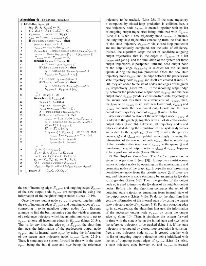
,newyv

Fig. 1: Extension of the graphs computed by the CL-RRT# algorithm.Trajectories in the output and state spaces are shown in orange and greencolors, respectively. Whenever a new node in the output space is added,then several incoming and outgoing edges are included to the graph in thevicinity of the new node, i.e., region colored with cyan.

also builds another graph Gσ , to store the state trajectoriescomputed by simulation of the closed-loop dynamics whena reference trajectory is tracked. Once a new node is addedto Gy after Extend, Replan is called to improve the existingsolution by propagating the new information (Line 7). Thedynamic system is simulated for different reference trajecto-ries as needed during the search process. The computed statetrajectories are added to the graph Gσ as new nodes alongwith the corresponding controls information.

Finally, when a predetermined maximum number of it-erations is reached, ConstrSolution extracts the spanningtree of Gy that contains the lowest-cost reference trajectories(Line 8). Algorithm 3 gives the details of ConstrSolution.

Algorithm 3: The ConstrSolution Solution Procedure1 ConstrSolution(S)2 (Gy,Gσ,Q,Qgoal)← S;3 (Vy, Ey)← Gy; X ← ∅;4 foreach vy ∈ Vy do5 σ ← vy.pσ.σ;6 vx ← StateNode(σ.back());7 Vx ← Vx ∪ {vx};8 vx,parent ← find(Vx,σ.front());9 if vx,parent = ∅ then

10 vx,parent ← StateNode(σ.front());11 Vx ← Vx ∪ {vx,parent};12 ex ← StateEdge(vx,parent, vx, σ);13 Ex ← Ex ∪ {ex};14 X ← X ∪ {σ.back()};15 return Tx = (Vx, Ex);

1) The Extend Procedure: The Extend procedure isgiven in Algorithm 4. It first extends the nearest output nodevy,nearest to the output sample y (Lines 4-5). The outputtrajectory that extends the nearest output node vy,nearesttowards the output sample y is denoted as rnew. The finaloutput point on the output trajectory rnew is denoted as ynew.If rnew is collision-free, then a new output node vy,new iscreated to represent the new output point ynew (Line 8), andthe following changes in the vicinity of vy,new on both graphsare shown in Fig. 1. The initial node is shown as a squarebox, the obstacles are shown in red color, and the graphs Gyand Gσ are shown in orange and green colors.

The members of the node vy,new are set as follows. First,Near finds the set of neighbor output nodes Vnear in theneighborhood of the new output point ynew (Line 9). Then,

Algorithm 4: The Extend Procedure#

1 Extend(S, Xgoal, y)2 (Gy,Gσ,Q,Qgoal)← S;3 (Vy, Ey)← Gy; (Vσ, Eσ)← Gσ;4 vy,nearest ← Nearest(Gy ,y);5 rnew ← Steer(vy,nearest.y,y);6 if ObstacleFree(rnew) then7 ynew ← rnew.back();8 vy,new ← OutNode(ynew);9 vy,new.h← ComputeHeuristic(ynew,Ygoal);

10 Vnear2← Near(Gy ,ynew,|Vy|) ∪ {vy,nearest};11 Ey,succ ← ∅; Ey,pred ← ∅;12 foreach vy,near ∈ Vnear2 do13 r ← Steer(ynew,vy,near.y);14 if ObstacleFree(r) then15 ey ← OutEdge(vy,new,vy,near,r);16 Ey,succ ← Ey,succ ∪ {ey};17 r ← Steer(vy,near.y,ynew);18 if ObstacleFree(r) then19 ey ← OutEdge(vy,near,vy,new,r);20 Ey,pred ← Ey,pred ∪ {ey};

21 V ′σ ← ∅; E′

σ ← ∅;22 foreach ey ∈ Ey,pred do23 vy,pred ← ey.tail;24 vσ,pred ← vy,pred.pσ;25 xpred ← vσ,pred.σ.back();26 σ ← Propagate(xpred,ey .r);27 if ObstacleFree(σ) then28 vσ,new ← TrajNode(σ,ey ,Ey,succ);29 eσ ← TrajEdge(vσ,pred,vσ,new,σ);30 V ′

σ ← V ′σ ∪ {vσ,new};

31 E′σ ← E′

σ ∪ {eσ};32 if vy,new.g > vy,pred.g+ Cost(σ) then33 vy,new.g← vy,pred.g+ Cost(σ);34 vy,new.py ← vy,pred;35 vy,new.pσ ← vσ,new;

36 Vy ← Vy ∪ {vy,new};Ey ← Ey ∪ Ey,succ ∪ Ey,pred;

37 Vσ ← Vσ ∪ V ′σ; Eσ ← Eσ ∪ E′

σ;38 Gy ← (Vy, Ey); Gσ ← (Vσ, Eσ);39 Q ← UpdateQueue(Q,vy,new);40 Qgoal ← UpdateGoal(Qgoal,vy,new,Xgoal);

41 return S ← (Gy,Gσ,Q,Qgoal);

the set of incoming edges Ey,pred and outgoing edges Ey,succof the new output node vy,new are computed by using theinformation of the neighbor output nodes (Lines 10-19).

Once the new output node vy,new is created together withthe set of incoming edges Ey,pred and outgoing edges Ey,succconnecting it to its neighbor output nodes Vnear, Extend

attempts to find the best incoming edge that yields a segmentof a reference trajectory which incurs minimum cost to get tovy,new among all incoming edges in Ey,pred (Lines 20-34).That is, for any incoming edge ey in Ey,pred, the algorithmfirst gets the information of the predecessor output nodevy,pred and its internal state xpred by using the informationof the parent state trajectory node vσ,pred (Lines 22-24).Then, it simulates the system forward in time with the statexpred being the initial state and ey.r being the reference

trajectory to be tracked, (Line 25). If the state trajectoryσ computed by closed-loop prediction is collision-free, anew trajectory node vσ,new is created together with its listof outgoing output trajectories being initialized with Ey,succ(Line 27). When a new trajectory node vσ,new is created,the outgoing state trajectories emanating from the final stateof the state trajectory vσ,new.σ via closed-loop predictionare not immediately computed, for the sake of efficiency.Instead, the algorithm keeps the set of candidate outgoingoutput trajectories, that is, the edges in Ey,succ, in a listvσ,new.outgoing, and the simulation of the system for theseoutput trajectories is postponed until the head output nodeof the output edge vσ,new.ey is selected for the Bellmanupdate during the Replan procedure. Once the new statetrajectory node vσ,new and the edge between the predecessorstate trajectory node vσ,pred and itself are created (Lines 27-28), they are added to the set of nodes and edges of the graphGσ , respectively (Lines 29-30). If the incoming output edgeey between the predecessor output node vy,pred and the newoutput node vy,new yields a collision-free state trajectory σthat incurs cost less than the current cost of vy,new, then,the g-value of vy,new is set with new lower cost, vy,pred andvσ,new are made the new parent output node and the newparent state trajectory node of vy,new (Lines 31-34).

After successful creation of the new output node vy,new, itis added to the graph Gy together with all of its collision-freeoutput edges (Line 36). Likewise, all trajectory nodes andedges created during the simulation of the system dynamicsare added to the graph Gσ (Line 37). Lastly, the priorityqueues, Q and Qgoal are updated accordingly by using theinformation of the new output node vy,new, that is, reorderingof the priorities after insertion of vy,new to the queue Q andreordering the goal output nodes in Qgoal if vy,new happensto be a goal output node (Lines 38-39).

2) The Replan Procedure: The Replan procedure isgiven in Algorithm 5 (see [3]). It improves cost-to-comevalues of output nodes by operating on the nonstationary andpromising nodes of the graph Gy . It pops the most promisingnonstationary node from the priority queue Q, if there areany, and this node is made stationary by assigning its g-valueto its g-value (Lines 5-6). Then, the g-value of the outputnode vy is used to improve the g-values of its neighbor outputnodes. Before this, the algorithm computes the set of alloutgoing state trajectories emanating from internal state ofthe output node v (Lines 9-16). To do so, the algorithm firstgets the information of the internal state x by using the parentstate trajectory node of vy (Lines 7-8). For any outgoing edgeey in vσ.outgoing, the algorithm first gets the informationof the successor output node vy,succ by using the outputedge ey (Line 10). Then, it simulates the system forwardin time with the state x being the initial state and ey.r beingthe reference trajectory to be tracked (Line 11). If the statetrajectory σ computed by closed-loop prediction is collision-free, a new trajectory node vσ,succ is created together withits list of outgoing output trajectories being initialized withthe set of outgoing output edges of vy,succ (Line 13). Also,a state trajectory edge between vσ and vσ,succ is created

(Line 14). Then, the new state trajectory node and edgeare tentatively added to the set of nodes and edges of thegraph Gσ (Lines 15-16). This continues until all candidateoutgoing output trajectories are processed in the closed-loopsimulation, then the list vy.outgoing is cleared up (Line17). All newly computed state trajectory nodes and edgesare added to the graph Gσ (Line 18).

For each outgoing state trajectory σ, Replan adds upits cost, incurred by reaching to the successor output nodevy,succ to the g-value of vy , and compare it with the currentg-value of vy,succ (Line 22). If the outgoing state trajectoryedge σ yields a lower cost than vy,succ, the g-value ofvy,succ is set with new lower cost, and vy and vσ,succ aremade the new parent output node and the new parent statetrajectory node of vy,succ, respectively (Lines 23-25). Last,the priority queues Q and Qgoal are updated by using theupdate information of the successor output node vy,succ, thatis, reordering of the priorities after updating the key value ofvy,succ to the queue Q and reordering the goal output nodesin Qgoal if vy,succ happens to be a goal output node (Lines26-27). These steps are repeated until there is no promisingnonstationary output node left in the priority queue Q, thatis, Q.top key() � Qgoal.top key().

Algorithm 5: Replan Procedure#

1 Replan(S, Xgoal)2 (Gy,Gσ,Q,Qgoal)← S;3 (Vσ, Eσ)← Gσ;4 while Q.top key() ≺ Qgoal.top key() do5 vy ← Q.pop();6 vy.g← vy.g;7 vσ ← vy.pσ;8 x← vσ.σ.back();9 foreach ey ∈ vσ.outgoing do

10 vy,succ ← ey.head;11 σ ← Propagate(x,ey .r);12 if ObstacleFree(σ) then13 vσ,succ ←

TrajNode(σ,ey ,outgoing(Gy ,vy,succ));14 eσ ← TrajEdge(vσ ,vσ,succ,σ);15 Vσ ← Vσ ∪ {vσ,succ};16 Eσ ← Eσ ∪ {eσ};

17 vσ.outgoing← ∅;18 Gσ ← (Vσ, Eσ);19 foreach vσ,succ ∈ succ(Gσ ,vσ) do20 σ ← vσ,succ.σ;21 vy,succ ← vσ,succ.ey.head;22 if vy,succ.g > vy.g+ Cost(σ) then23 vy,succ.g← vy.g+ Cost(σ);24 vy,succ.py ← vy;25 vy,succ.pσ ← vσ,succ;26 Q ← UpdateQueue(Q,vy,succ);27 Qgoal ←

UpdateGoal(Qgoal,vy,succ,Xgoal);

28 return S ← (Gy,Gσ,Q,Qgoal);

The auxiliary procedures in Extend and Replan areshown in Algorithm 6. UpdateQueue maintains the pri-ority queue Q whenever a new output node is created orkey value of an output node that is already in the queue is

updated. During a call to UpdateQueue with the priorityqueue Q and the output node vy , there are three possiblecases. First, if vy is a nonstationary output node, that is,vy.g 6= vy.g, key value of vy is updated and priorities in thequeue are reordered (Line 3). Second, if vy is a nonstationaryoutput node and it is not in the queue, then it is inserted tothe queue Q with its key value (Line 5). Third, if vy is astationary output node, that is, vy.g = vy.g, and it is in thequeue Q, then, it is removed from the queue Q (Line 7).

Algorithm 6: Auxiliary Procedures#

1 UpdateQueue(Q, vy)2 if vy.g 6= vy.g and vy ∈ Q then3 Q.update(vy ,Key(vy));

4 else if vy.g 6= vy.g and vy /∈ Q then5 Q.insert(vy ,Key(vy));

6 else if vy.g = vy.g and vy ∈ Q then7 Q.remove(vy);

8 return Q;

9 UpdateGoal(Qgoal, vy,Ygoal)10 vσ ← vy.pσ;11 x← vσ.σ.back();12 if x ∈ Xgoal then13 if vy ∈ Qgoal then14 Qgoal.update(vy ,Key(vy));

15 else16 Qgoal.insert(vy ,Key(vy));

17 return Qgoal;

18 Key(vy)19 return k = (vy.g+ vy.h, vy.h);

Algorithm 7 gives constructor procedures for node andedge data structures used in the CL-RRT#.

Algorithm 7: Node and Edge Constructor Procedures#

1 OutNode(y)2 vy.y ← y;3 vy.g←∞; vy.g←∞;4 vy.h← 0;5 vy.py ← ∅; vy.pσ ← ∅;6 return vy;

7 OutEdge(vy,from, vy,to, r)8 ey.tail← vy,from;9 ey.head← vy,to;

10 ey.r ← r;11 return ey;

12 TrajNode(σ, ey, Ey)13 vσ.σ ← σ;14 vσ.ey ← ey;15 vσ.outgoing← Ey;16 return vσ;

17 TrajEdge(vσ,from, vσ,to, σ)18 eσ.tail← vσ,from;19 eσ.head← vσ,to;20 eσ.σ ← σ;21 return eσ;

22 StateNode(x)23 vx.x← x;24 return vx;

25 StateEdge(vx,from, vx,to, σ)26 ex.tail← vx,from;27 ex.head← vx,to;28 ex.σ ← σ;29 return ex;

C. Properties of the Algorithm

The CL-RRT# algorithm provides both dynamic feasi-bility guarantees, that is, the lowest-cost reference trajectorycomputed by the algorithm can be tracked by the low-levelcontroller, and asymptotic optimality guarantees, that is, thelowest-cost reference trajectory computed by the algorithmconverges to the optimal reference trajectory almost surely.The former property is an immediate result of using closed-

loop prediction during the search phase. During the extensionof the graph Gy , if some segments of a reference trajectorycan not be tracked, that is, is not dynamically feasible, thecorresponding state trajectory is not stored in the graphGσ constructed by the algorithm. The former property isdue to the asymptotic optimality property of the RRT#

algorithm [3]. The proposed algorithm incrementally grows agraph Gy in the output space in a similar fashion as the RRGalgorithm does [6]. Therefore, the lowest-cost path encodedin Gy converges to the optimal output trajectory in the outputspace almost surely. In addition, the lowest-cost outputtrajectory encoded in the graph Gy is extracted at the end ofeach iteration in a similar fashion as the RRT# algorithmdoes. Given the cost function that associates each edge inGy with a non-negative cost values being monotonic andbounded, the proposed algorithm is asymptotically optimal.

IV. NUMERICAL STUDY

The proposed algorithm is evaluated on two scenarioswhere a nonholonomic, wheeled vehicle, modeled as aunicycle, travels along a track. The motion equations are

x1 = x4 sin(x3), x2 = x4 cos(x3), x3 = u1, x4 = u2,

y1 = x1, y2 = x2,

where x1, x2 are the Cartesian coordinates of the vehicle,x3 is the heading angle, x4 is the translational velocity ,and u1, u2 are the controls for the angular and translationalvelocity. Each control input takes values in an interval, thatis, ui ∈ [uli, u

ui ]. A pure-pursuit controller tracks a given

reference path [1]. The heading command is generated byfollowing a look-ahead point on a given reference path. Thespeed command is given as a desired speed vcrs, which istracked by a proportional controller.

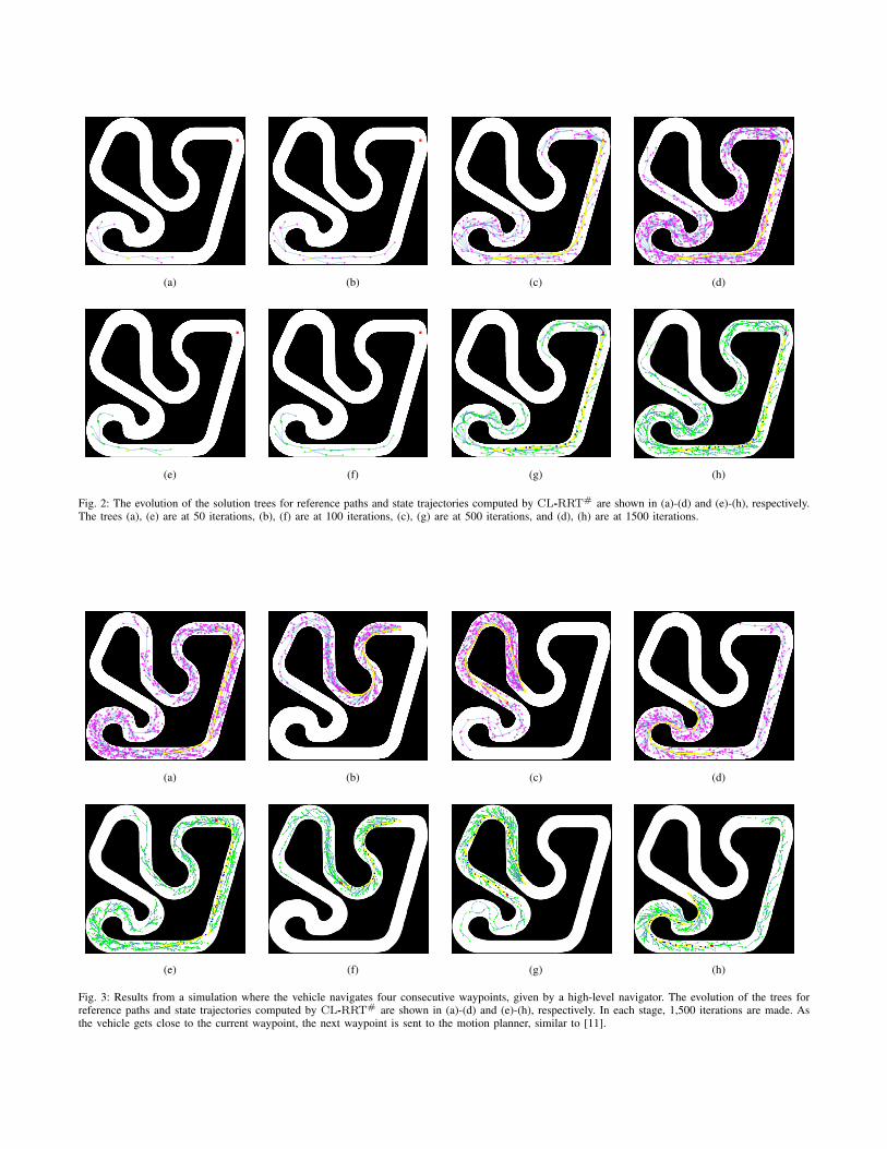
First, the objective is point-to-point navigation in thecounter-clockwise direction on a race track, while min-imizing the Euclidean path length. The track size is(100m×100m) and the origin is located at its center.CL-RRT#executed for 1,500 iterations. Fig. 2 shows theresulting tree at different stages. Initially, the vehicle is at(−25,−45), with zero heading angle and zero speed (yellowsquare at bottom-left). The task is to move to (48, 33) (redsquare at top-right). As seen in Figs. 2(a)-(d), the algorithmincrementally grows a graph in the output space (x1, x2).Each path in the graph corresponds to a reference path, usedas an input to the closed-loop system. CL-RRT#quicklycomputes a long reference path. Then, it seeks alternativepaths of the graph as more information is explored andimproves the existing solution if closed-loop simulation of anew reference path yields lower cost. The nodes and edges ofthe graph correspond to waypoints and straight line segments.The lowest-cost path is shown in yellow. The value is 127.2.Figs. 2(e)-(h) shows the state trajectories, computed duringclosed-loop simulation in CL-RRT#.

In the second scenario, the goal is to recursively navigatethe vehicle on the race track. The vehicle is tasked to navigatesequentially to a set of waypoints, presumably coming from ahigh-level navigator. In each stage, the CL-RRT#algorithm

was executed for 1,500 iterations to find a motion planfrom the current state of the vehicle to a desired nextwaypoint. Each next waypoint is sent to the motion planneras the vehicle gets close to the current waypoint, similarto [11]. In this simulation, the vehicle is tasked to navigatefour waypoints sequentially. The solution trees of referencepaths and corresponding state trajectories for each step areshown in Fig. 3. As seen during simulations, leveraging thedynamics information of the vehicle during the search phaseallows to construct dynamically feasible paths and avoidshortest paths that pass close to the boundary of the track.

V. CONCLUSION

We presented a new asymptotically optimal motion-planning algorithm, called CL-RRT#, using closed-loopprediction for trajectory generation. The approach is a hybridof the CL-RRT and the RRT# algorithms. It incrementallygrows a graph of reference trajectories, used as inputs to alow-level tracking controller, and chooses the one that yieldsthe lowest-cost state trajectory of the closed-loop system.CL-RRT# provides dynamic feasibility by construction andensures asymptotic optimality, that is, it finds the optimalreference trajectory given controller. Simulation results on anonholonomic system showed the efficacy of the approach.

REFERENCES

[1] O. Amidi. Integrated mobile robot control. Technical Report CMU-RI-TR-90-17, Carnegie Mellon University, Robotics Institute, May 1990.

[2] O. Arslan, E. A. Theodorou, and P. Tsiotras. Information-theoreticstochastic optimal control via incremental sampling-based algorithms.In IEEE Symp. Adaptive Dynamic Programming and ReinforcementLearning, pages 1–8, 2014.

[3] O. Arslan and P. Tsiotras. Use of relaxation methods in sampling-based algorithms for optimal motion planning. In IEEE Int. Conf.Robotics and Automation, pages 2413–2420, 2013.

[4] O. Arslan and P. Tsiotras. Dynamic programming guided explorationfor sampling-based motion planning algorithms. In IEEE Int. Conf.Robotics and Automation, pages 4819–4826, 2015.

[5] O. Arslan and P. Tsiotras. Dynamic programming principles forsampling-based motion planners. In ICRA Optimal Robot MotionPlanning Workshop, 2015.

[6] S. Karaman and E. Frazzoli. Optimal kinodynamic motion planningusing incremental sampling-based methods. In 49th IEEE Conf.Decision and Control, pages 7681–7687, 2010.

[7] S. Karaman and E. Frazzoli. Sampling-based algorithms for optimalmotion planning. Int. J. Robotics Research, 30(7):846–894, 2011.

[8] S. Karaman, M. R. Walter, A. Perez, E. Frazzoli, and S. Teller.Anytime motion planning using the RRT*. In IEEE Int. Conf. Roboticsand Automation, pages 1478–1483, 2011.

[9] S. Koenig, M. Likhachev, and D. Furcy. Lifelong planning A*.Artificial Intelligence Journal, 155(1-2):93–146, 2004.

[10] J. J. Kuffner, S. Kagami, K. Nishiwaki, M. Inaba, and H. In-oue. Dynamically-stable motion planning for humanoid robots. Au-tonomous Robots, 12(1):105–118, 2002.

[11] Y. Kuwata, J. Teo, S. Karaman, G. Fiore, E. Frazzoli, and J. P.How. Motion planning in complex environments using closed-loopprediction. In AIAA Guidance, Navigation, and Control Conf., 2008.

[12] S. M. LaValle. Planning Algorithms. Cambridge University Press,2006.

[13] S. M. LaValle and J. J. Kuffner, Jr. Randomized kinodynamic planning.Int. J. Robotics Research, 20(5):378–400, May 2001.

[14] J. Leonard et al. A perception-driven autonomous urban vehicle. J.Field Robotics, 25(10):727–774, 2008.

[15] J. H. Reif. Complexity of the movers problem and generalizations. InProc. IEEE Conf. Foundations of Computer Science, pages 421–427,1979.

[16] R. Vinter. Optimal Control. Birkhauser, Boston, MA, 2010.

(a) (b) (c) (d)

(e) (f) (g) (h)

Fig. 2: The evolution of the solution trees for reference paths and state trajectories computed by CL-RRT# are shown in (a)-(d) and (e)-(h), respectively.The trees (a), (e) are at 50 iterations, (b), (f) are at 100 iterations, (c), (g) are at 500 iterations, and (d), (h) are at 1500 iterations.

(a) (b) (c) (d)

(e) (f) (g) (h)

Fig. 3: Results from a simulation where the vehicle navigates four consecutive waypoints, given by a high-level navigator. The evolution of the trees forreference paths and state trajectories computed by CL-RRT# are shown in (a)-(d) and (e)-(h), respectively. In each stage, 1,500 iterations are made. Asthe vehicle gets close to the current waypoint, the next waypoint is sent to the motion planner, similar to [11].