Optimal Model Reduction Using Genetic Algorithms and Particle Swarm Optimization

University of Sharjah College of Engineering

Electrical and Computer Engineering Department

Optimal Model Reduction Using Genetic Algorithms

and Particle Swarm Optimization

by

REEM IZZELDIN SALIM

Supervisor

Professor Maamar Bettayeb

Program: Electrical and Electronics Engineering

16-04-2009

Optimal Model Reduction Using Genetic Algorithms

and Particle Swarm Optimization

by

Reem Izzeldin Salim

A thesis submitted in partial fulfillment of the requirements for the degree of Master of

Science in the Department of Electrical and Computer Engineering, University of Sharjah

Approved by:

Maamar Bettayeb ……………………………………………………. Chairman

Professor of Electrical and Electronics Engineering, University of Sharjah

Abdulla Ismail Abdulla ………………………………………………… Member

Professor of Electrical Engineering, United Arab Emirates University

Karim Abed Meraim ………………………………………………… Member

Associate Professor of Electrical and Electronics Engineering, University of Sharjah

Mohamed Saad ……………………………………………………… Member

Assistant Professor of Computer Engineering, University of Sharjah

16-04-2009

To my parents

“O Lord, bestow on them the Mercy even as they cherished me in childhood.” (The Holy Quran 17: 24)

And to my dear husband, Faris

I

Acknowledgement

ll praise and thanks are due to Almighty Allah, Most Gracious; Most Merciful,

for the immense mercy which have resulted in accomplishing this research. May

peace and blessings be upon prophet Muhammad (PBUH), his family and his companions.

I would like to thank my thesis Supervisor, Professor Maamar Bettayeb for his

continuous support and guidance throughout my research. Without his substantial knowledge and

experience, I would not have been able to complete this work.

I would like to thank my examining committee, Professor Abdulla Ismail Abdulla, Dr.

Karim Abed Meraim and Dr. Mohamed Saad for taking the time to review my study and for their

valuable input.

I would also like to acknowledge Mr. Mohammed Ubaid for taking the time to help me

overcome some of the many difficulties I encountered using MATLAB.

A

II

I would also like to express my sincere gratitude to my dear parents and my husband

Faris for being there for me in good and bad. They have supported me in everything that I have

endeavored, and their continuous encouragement always lifted up my self confidence whenever I

encountered problems. Words fall short in conveying my gratitude towards them. A prayer is the

simplest means I can repay them.

Finally, I would like to thank everybody who was important to the successful realization

of this thesis, and I apologize for not mentioning everyone personally.

III

Table of Contents

Acknowledgement ..................................................................................................................... I

Table of Contents ...................................................................................................................... III

List of Tables ........................................................................................................................... VIII

List of Figures ............................................................................................................................ X

Abstract ..................................................................................................................................... XV

Chapter 1: Introduction ........................................................................................................... 1

1.1 Model Reduction ..................................................................................................... 5

1.2 Purpose of the Study ................................................................................................ 6

1.3 Study Method .......................................................................................................... 7

IV

Chapter 2: Literature Review .................................................................................................. 9

2.1 Classical Model Reduction ...................................................................................... 9

2.2 Optimal Model Reduction ..................................................................................... 10

2.2.1 H∞ Norm Model Reduction ......................................................................... 14

2.2.2 H2 Norm Model Reduction ....................................................................... 16

2.2.3 L1 Norm Model Reduction .......................................................................... 18

2.3 Previous Studies ...................................................................................................... 19

Chapter 3: Evolutionary Algorithms ...................................................................................... 23

3.1 Genetic Algorithms ................................................................................................. 24

3.2 Particle Swarm Optimization .................................................................................. 27

Chapter 4: H2 Norm Model Reduction ................................................................................... 31

4.1 GA Approach Results .............................................................................................. 35

4.2 PSO Approach Results ............................................................................................ 40

4.3 Comparative Study of the Two Approaches ........................................................... 44

4.3.1 Steady State Errors and Norms .................................................................. 46

4.3.2 Impulse Responses and Initial Values ........................................................ 47

4.3.3 Step Responses ........................................................................................... 50

4.3.4 Frequency Responses ................................................................................. 52

4.4 GA and PSO H2 Model Reduction Approaches versus Previous Studies ................ 55

4.4.1 Maust and Feliachi ...................................................................................... 55

4.4.2 Yang, Hachino, and Tsuji ............................................................................ 56

V

Chapter 5: H∞ Norm Model Reduction ................................................................................... 65






5.3.3 Step Responses ........................................................................................... 76


5.4 PSO H∞ Norm Model Reduction Approach versus Previous Studies ..................... 80

Chapter 6: L1 Norm Model Reduction ................................................................................... 84






6.3.3 Step Responses ........................................................................................... 93


6.4 GA and PSO L1 Model Reduction Approaches versus Previous Studies ................ 97

Chapter 7: Hybrid Norm Model Reduction ........................................................................... 99

7.1 Hybrid between H2 and H∞ Norms ......................................................................... 100

7.1.1 GA Approach Results ................................................................................. 100

VI

7.1.2 PSO Approach Results ................................................................................101

7.1.3 Comparative Study of the Two Approaches ................................................102

7.1.3.1 Steady State Errors and Norms ......................................................102

7.1.3.2 Impulse Responses and Initial Values ............................................103

7.1.3.3 Step Responses ...............................................................................106

7.1.3.4 Frequency Responses ......................................................................108

7.2 Hybrid between L1, H2 and H∞ Norms ................................................................... 110

7.2.1 GA Approach Results ..................................................................................111

7.2.2 PSO Approach Results ................................................................................112

7.2.3 Comparative Study of the Two Approaches ................................................113

7.2.3.1 Steady State Errors and Norms ......................................................113

7.2.3.2 Impulse Responses and Initial Values .......................................... 114

7.2.3.3 Step Responses .............................................................................. 117

7.2.3.4 Frequency Responses .....................................................................119

7.3 Comparison between the Two Hybrid Norms ........................................................ 121

Chapter 8: Conclusion & Future Work ................................................................................ 123

References ..................................................................................................................................130

List of Accepted/Submitted Papers from Thesis Work ........................................................ 144

VII

Appendices ................................................................................................................................ i

Appendix 1: Thesis MATLAB Code ...................................................................................... ii

Appendix 2: GA Functions ..................................................................................................... ix

2.1 L1 Norm Function .............................................................................................. ix

2.2 H2 Norm Function .............................................................................................. x

2.3 H∞ Norm Function ............................................................................................. x

2.4 Hybrid Norm Function ...................................................................................... xi

Appendix 3: PSO Functions .................................................................................................. xiii

3.1 L1 Norm Function ............................................................................................. xiii

3.2 H2 Norm Function ............................................................................................ xiv

3.3 H∞ Norm Function ............................................................................................ xv

3.4 Hybrid Norm Function ...................................................................................... xv

3.5 H2 Norm with Time-Delay Function ............................................................... xvi

VIII

List of Tables

Table 4.1 Wilson: GA Performance for Different Population Sizes ................................. 39

Table 4.2 Wilson: PSO Performance for Different Swarm Sizes ...................................... 43

Table 4.3 Wilson: SSE and Norms of the H2 Norm MR approach ................................... 46

Table 4.4 Boiler: SSE and Norms of the H2 Norm MR approach ..................................... 46

Table 4.5 H2 Norms of Yang et al.’s 6th order example ..................................................... 58

Table 5.1 Wilson: SSE and Norms of the H∞ Norm MR approach ................................... 72

Table 5.2 Boiler: SSE and Norms of the H∞ Norm MR approach .................................... 72

Table 5.3 Weighted H∞ Norm Model Reduction Results .................................................. 83

Table 6.1 Wilson: SSE and Norms of the L1 Norm MR approach .................................... 89

IX

Table 6.2 Boiler: SSE and Norms of the L1 Norm MR approach ..................................... 89

Table 7.1 Wilson: SSE and Norms of the first Hybrid Norm MR approach .......................102

Table 7.2 Boiler: SSE and Norms of the first Hybrid Norm MR approach ...................... 102

Table 7.3 Wilson: SSE and Norms of the second Hybrid Norm MR approach .................113

Table 7.4 Boiler: SSE and Norms of the second Hybrid Norm MR approach ...................113

Table 8.1 Summary of the Wilson System Results ........................................................... 126

Table 8.2 Summary of the Boiler System Results ............................................................ 127

X

List of Figures

Figure 3.1 Roulette Wheel ................................................................................................... 26

Figure 3.2 Genetic Algorithm Flowchart ............................................................................ 27

Figure 4.1 Wilson: Convergence Rate of the GA for different population sizes ................ 39

Figure 4.2 Wilson: Convergence Rate of the PSO for different swarm sizes ..................... 43

Figure 4.3 Wilson: Convergence Rate of GA and PSO ...................................................... 44

Figure 4.4 Boiler: Convergence Rate of GA and PSO ....................................................... 45

Figure 4.5 Wilson: Impulse Responses of the H2 Norm MR approach .............................. 47

Figure 4.6 Wilson: Initial Values of the H2 Norm MR approach ....................................... 48

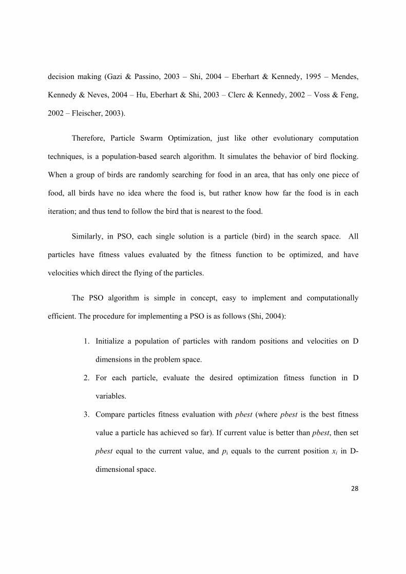
Figure 4.7 Boiler: Impulse Responses of the H2 Norm MR approach ................................ 49

XI

Figure 4.8 Boiler: Initial Values of the H2 Norm MR approach ......................................... 50

Figure 4.9 Wilson: Step Responses of the H2 Norm MR approach .................................... 51

Figure 4.10 Boiler: Step Responses of the H2 Norm MR approach ..................................... 52

Figure 4.11 Wilson: Frequency Responses of the H2 Norm MR approach .......................... 53

Figure 4.12 Boiler: Frequency Responses of the H2 Norm MR approach ............................ 54

Figure 4.13 Yang: Impulse Responses of the 1st order reduced models ....................................... 59

Figure 4.14 Yang: Step Responses of the 1st order reduced models ............................................ 59

Figure 4.15 Yang: Frequency Responses of the 1st order reduced models ................................... 60

Figure 4.16 Yang: Impulse Responses of the 2nd order reduced models ...................................... 60

Figure 4.17 Yang: Step Responses of the 2nd order reduced models ........................................... 61

Figure 4.18 Yang: Frequency Responses of the 2nd order reduced models .................................. 61

Figure 4.19 Yang: Impulse Responses of the 3rd order reduced models ...................................... 62

Figure 4.20 Yang: Step Responses of the 3rd order reduced models ............................................ 62

Figure 4.21 Yang: Frequency Responses of the 3rd order reduced models ................................... 63

Figure 4.22 Yang: Impulse Responses of the 4th order reduced models ....................................... 63

Figure 4.23 Yang: Step Responses of the 4th order reduced models ............................................ 64

Figure 4.24 Yang: Frequency Responses of the 4th order reduced models ................................... 64

XII



Figure 5.3 Wilson: Impulse Responses of the H∞ Norm MR approach .............................. 73

Figure 5.4 Wilson: Initial Values of the H∞ Norm MR approach ....................................... 74

Figure 5.5 Boiler: Impulse Responses of the H∞ Norm MR approach ............................... 75

Figure 5.6 Boiler: Initial Values of the H∞ Norm MR approach ........................................ 76

Figure 5.7 Wilson: Step Responses of the H∞ Norm MR approach ................................... 77

Figure 5.8 Boiler: Step Responses of the H∞ Norm MR approach ..................................... 78

Figure 5.9 Wilson: Frequency Responses of the H∞ Norm MR approach .......................... 79

Figure 5.10 Boiler: Frequency Responses of the H∞ Norm MR approach ........................... 80



Figure 6.3 Wilson: Impulse Responses of the L1 Norm MR approach ............................... 90

Figure 6.4 Wilson: Initial Values of the L1 Norm MR approach ........................................ 91

Figure 6.5 Boiler: Impulse Responses of the L1 Norm MR approach ................................ 92

Figure 6.6 Boiler: Initial Values of the L1 Norm MR approach ......................................... 93

Figure 6.7 Wilson: Step Responses of the L1 Norm MR approach .................................... 94

XIII

Figure 6.8 Boiler: Step Responses of the L1 Norm MR approach ...................................... 95

Figure 6.9 Wilson: Frequency Responses of the L1 Norm MR approach ........................... 96

Figure 6.10 Boiler: Frequency Responses of the L1 Norm MR approach ............................ 97

Figure 7.1 Wilson: Impulse Responses of the first Hybrid Norm MR approach ................ 103

Figure 7.2 Wilson: Initial Values of the first Hybrid Norm MR approach ......................... 104

Figure 7.3 Boiler: Impulse Responses of the first Hybrid Norm MR approach ................. 105

Figure 7.4 Boiler: Initial Values of the first Hybrid Norm MR approach .......................... 106

Figure 7.5 Wilson: Step Responses of the first Hybrid Norm MR approach ..................... 107

Figure 7.6 Boiler: Step Responses of the first Hybrid Norm MR approach ....................... 108

Figure 7.7 Wilson: Frequency Responses of the first Hybrid Norm MR approach ............. 109

Figure 7.8 Boiler: Frequency Responses of the first Hybrid Norm MR approach .............. 110

Figure 7.9 Wilson: Impulse Responses of the second Hybrid Norm MR approach ............ 114

Figure 7.10 Wilson: Initial Values of the second Hybrid Norm MR approach .................... 115

Figure 7.11 Boiler: Impulse Responses of the second Hybrid Norm MR approach ............ 116

Figure 7.12 Boiler: Initial Values of the second Hybrid Norm MR approach ..................... 117

Figure 7.13 Wilson: Step Responses of the second Hybrid Norm MR approach ................. 118

Figure 7.14 Boiler: Step Responses of the second Hybrid Norm MR approach .................. 119

XIV

Figure 7.15 Wilson: Frequency Responses of the second Hyb. Norm MR approach ............120

Figure 7.16 Boiler: Frequency Responses of the second Hyb. Norm MR approach ..............121

XV

Abstract

he mathematical modeling of most physical systems, such as telecommunication

systems, transmission lines and chemical reactors, results in complex high order

models. The complexity of the models imposes major difficulties in analysis, simulation and

control designs. Model reduction helps to reduce these difficulties. Several analytical model

reduction techniques have been proposed in the literature over the past few decades, to

approximate high order linear dynamic systems. However, most of the optimal techniques lead to

computationally demanding, time consuming, iterative procedures that usually result in non-

robustly stable models with poor frequency response resemblance to the original high order

model in some frequency ranges. Genetic Algorithms (GA) and Particle Swarm Optimization

(PSO) methods have proved to be excellent optimization tools. Therefore, the aim of this thesis

is to use GA and PSO to solve complex model reduction problems with no available analytic

solutions, and help obtain globally optimized reduced order models.

T

XVI

Keywords: Model Reduction, Optimal Approximation, L1 Norm, H2 Norm, H∞ Norm,

Hybrid Norm, Evolutionary Algorithm, Genetic Algorithm, Particle Swarm Optimization, Global

Solution.

Chapter 1

Introduction

he mathematical modeling of most physical systems, such as telecommunication

systems, transmission lines and chemical reactors, results in infinite dimensional

models. Using engineering tools we can still roughly represent those systems with approximate

finite dimensional models (Al-Saggaf & Bettayeb, 1993).

However, complex large-scale systems usually require high dimensional models to well-

represent them. Analysis, simulation and design methods based on this high order model may

eventually lead to complicated control strategies requiring very complex logic or large amounts

of computation (Bettayeb, 1981).

Model Reduction is a branch of systems and control theory, which studies properties of

dynamical systems in order to reduce their complexity, while preserving (to the possible extent)

T

2

their input-output behavior (Massachusetts Institute of Technology, 2009). Specifically, the use

of low order models lead to the following desired properties (Bettayeb, 1981):

1. Simple design and analysis: Feedback design of high order models often lead to high

dimensional control laws which then result in complex feedback structures. These

structures are simplified if one starts with reduced models resulting in low order control

laws. Also, in identification problems, one is asked to derive a preferably low order

model given noisy input output data.

2. Computational advantage: In linear quadratic control and estimation problems, the

computation of the optimal controller and observer amount to solving a quadratic matrix

Ricatti equation. The size of this matrix is precisely the order of the model. Thus, the

computational requirements on simplified models will be much lower since computation

time and complexity on this quadratic equation rise at a rate greater than linearly with the

problem dimension.

3. Simplicity of simulation: Simulation of models can be used in understanding some

properties of the system. Very often simulation of lower order models adequately

displays the important dynamics of the physical system. In real time control of complex

systems, simple simulation is often necessary. It is also desirable for simple hardware

implementation of the model.

Model Reduction is also important in filter design. For example, one is asked to

approximately realize a non-realizable ideal filter by low order filters (Bettayeb, 1981).

3

Another important consideration is the quality of the reduced order model. The accuracy

measure of the approximation should in some concrete way take into consideration the difference

in behavior between the original system and the reduced order model (Bettayeb, 1981).

Different Norms are used for the formulation of the model reduction problem. Of course,

one has to be aware of the following facts (Bettayeb, 1981):

1. The use of different norms gives rise to different approximations. A good approximation

in one norm is not necessarily good in another norm. Various norms are therefore chosen

depending on each individual application.

2. Close approximations based on time domain criteria do not necessarily translate into

good frequency domain approximations.

The Model Reduction problem is a tradeoff between two conflicting desirable objectives

(Bettayeb, 1981):

1. To derive from the high order system a model as simple (low order) as possible

(complexity).

2. The low order model is reasonably close to the original system (accuracy).

Assume one has a device, and that (using finite-difference discretization or any other

modeling technique) its description is obtained in the form of a differential equation, or a transfer

function. Usually, this will result in a system of a very high order, evidently redundant for

representing some properties of interest. Model Reduction is used to create the smallest possible

4

model while preserving the system’s input-output behavior (Massachusetts Institute of

Technology, 2009).

For example, consider a transmission line. We can obtain its dynamical model by

discretizing its length, representing each small piece as a small resistor, inductor plus capacitor to

the ground, and then create a description using nodal voltage analysis. By solving this system for

any given input, the voltage distribution at any given point of the line will be known. Assume

that we are not interested in knowing the exact distribution of the voltage along the line, but

rather interested in how the signal is transmitted through the line, i.e., we need to know the

dependence of the voltage and the current at one end of the line on the voltage and the current at

the other end of the line. In order to simulate this line efficiently, especially if this line is part of

some complex circuit, a simplified representation of this line is required. Model Reduction

produces this simplified representation (Massachusetts Institute of Technology, 2009).

Historically, system modeling has been something of an art, requiring either special

knowledge of the system being considered, or a certain “intuition” into the modeling process

itself. The resulting system models may be extremely complex. For example, in the field of

Computational Fluid Dynamics (CFD), flow systems are sometimes described by literally

millions of dynamic state equations. There exist many techniques in practice for reducing the

complex models and creating a useful low order system model. Regardless of which modeling

approach is used, the process always yields some modeling error (Hartley, et al, 1998).

5

1.1 Model Reduction:

Considering the following general state space model representation of a single-input-

single-output (SISO) time-invariant linear continuous time system:

(1.1)

where x(t) is the state, u(t) is the input, and y(t) is the output. This state space model can be

represented by the following nth order transfer function:

(1.2)

The aim of optimal model reduction is to obtain a reduced order state space model

representation or a reduced order transfer function of the system that well represents the original

system:

(1.3)

(1.4)

In this thesis, three different model reduction problems will be investigated using Genetic

Algorithms (GA) and Particle Swarm Optimization (PSO). These problems are H2 norm, H∞

norm and L1 norm Model Reduction.

The H∞ norm is defined as:

6

∞ max | |

max . (1.5)

where:

E(s) = G(s) – Gr(s) (1.6)

and the H2 norm is defined as:

| | ∞∞ (1.7)

The L1 norm on the other hand is defined as:

| |∞ (1.8)

where e(t) is the impulse response difference between the original system and the reduced

system:

(1.9)

1.2 Purpose of the Study:

The models of many modern control systems are of high order and thus are very

complex. This complexity will impose difficulties in analysis, simulation and control designs.

Performing model reduction will help reduce those difficulties.

7

In model reduction, it is important that the reduced order model provides close

approximation to the original high order system for different types of inputs, while yielding the

minimum steady state error and preserving the stability characteristics of the original high order

system.

Several analytical model reduction techniques have been proposed in the literature over

the past few decades. However, most of the optimal techniques follow time-consuming, iterative

procedures that usually result in non-robustly stable models with poor frequency response

resemblance to the original high order model in some frequency ranges.

Genetic Algorithms (GA) and Particle Swarm Optimization (PSO) methods have proved

to be excellent optimization tools in the past few years. The use of such search-based

optimization algorithms in Model Reduction ensures that all the Model Reduction objectives are

realized with minimal computational effort. Therefore, the aim of this thesis will be to use GA

and PSO to solve model reduction problems, and help obtain a globally optimized nominal

model. The thesis will also compare the results of the two approaches with the analytical

solutions obtained by other researchers in previous works and draw a conclusion.

1.3 Study Method:

This study uses MATLAB 7.0 to build the GA and PSO model reduction approaches

based on H2 norm, H∞ norm and L1 norm1. MATLAB 7.0’s embedded GA toolbox was used to

build the GA model reduction approach. A PSO toolbox on the other hand was not introduced 1 All MATLAB Codes are presented in the Appendices.

8

into MATLAB yet. However, Birge (2003) introduced a reliable toolbox (PSOt) that has been

used by many researchers to implement and study their different PSO applications. Revision 3.3

of the PSOt toolbox, dated 18/02/2006, was used to build the proposed PSO model reduction

approach of this thesis work with slight modifications.

The GA and PSO approaches will be tested on different original models with different

orders, in order to obtain optimally reduced models. The results of both approaches will be

compared to results obtained by other researchers in the area. The two approaches will also be

compared to one another in order to conclude which of the two approaches yields better results.

The comparison process will be based on: impulse response, step response, frequency response,

steady state values, initial values, H2 norm, H∞ norm and L1 norm.

Chapter 2

Literature Review

odel reduction has been an attractive research area in the past few decades.

This chapter summarizes the classical and optimal model reduction approaches

as well as the previous model reduction studies that used Genetic Algorithms and Particle Swarm

Optimization.

2.1 Classical Model Reduction:

Model Reduction started in 1966 when Davison (1966, 1967) presented “The Modal

Analysis” approach using state space techniques. Chidambara (1967, 1969) then offered several

modifications to Davison’s approach. Later on several researchers started to add their imprints in

the area when, Chen and Shieh (1968) used frequency domain expansions; Gibilaro and Lees

(1969) matched the moments of the impulse response; Hutton and Friedland (1975) used the

M

10

Routh approach for high frequency approximation which was modified by Langholz and

Feinmesser (1978); and then Pinguet (1978) showed that all those methods have state space

reformulations.

2.2 Optimal Model Reduction:

The model reduction approaches cited in the previous section did not consider optimality.

It was not until 1970, that optimal model reduction was considered by Wilson (1970, 1974). He

used an H2 norm model reduction approach based on the minimization of the integral squared

impulse response error between the full and reduced order models.

Given an nth order state space representation of a system in the form:

(2.1)

where x is an n × 1 vector, u is a p × 1 vector and y is an m × 1 vector, Wilson aimed to find a

reduced order state space representation of the system of order r, where m < r < n:

(2.2)

The following function represents Wilson’s cost function to be minimized:

(2.3)

where he sets Q to be the m × m identity matrix, and e(t) is the error signal:

11

(2.4)

By substituting eq. (2.4) in eq. (2.3):

(2.5)

where

(2.6)

Minimization of eq. (2.5) leads to the following Lyapunov equations:

0 (2.7)

0 (2.8)

Where R and P are unique positive definite solutions of these linear Lyapunov equations and

hence can be solved in closed form:

00 (2.9)

If P and R are partitioned compatibly with F as:

(2.10)

Then the necessary conditions for optimality gives:

(2.11)

12

(2.12)

(2.13)

Note that eqs. (2.7) and (2.8) are nonlinear in the unknown reduced order matrices Ar, Br

and Cr. This non-linearity is the severe drawback of Wilson’s method. The method is

computationally demanding, and requires iterative minimization algorithms which suffer from

many difficulties such as the choice of starting guesses, convergence, and multiple local minima.

In the early 1980s; Obinata and Inooka (1976, 1983) and Eitelberg (1981) in other

approachs, minimized the equation error that leads to closed form solutions. The L1-norm

minimization approach was then presented by El-Attar and Vidyasagar (1978).

The classical approach to model reduction dealt only with eigenvalues. However, in

1981, Moore (1981) published a paper presenting a revolutionary way of looking at model

reduction by showing that the ideal platform to work from is that when all states are as

controllable as they are observable. This gave birth to “Balanced Model Reduction”, where the

concept of dominance is no longer associated with eigenvalues, but rather with the degree of

controllability and observability of a given state.

Moore’s approach aims at changing the form of the system’s state space model

representation, by the use of a certain transformation matrix, into a balanced model with the

transformed states being as controllable as they are observable, and ordered from strongly

controllable and observable to weakly controllable and observable.

13

Since the output depends on both the controllability and the observability of a state; the

states which are weakly controllable and observable will have little effect on the output, and

thus, discarding them will not affect the output very much. This is what motivated Moore to

develop his approach. Pernebo and Silverman (1982) showed that the stability of this reduced

model is assured if the original system was also stable. However, Moore’s approach still suffered

from steady state errors (Al-Saggaf & Bettayeb, 1993).

Hankel-norm reduction which was studied by Silverman and Bettayeb (1980), Bettayeb,

Silverman and Safonov (1980), Kavranoğlu and Bettayeb (1982, 1993a), and Glover (1984) on

the other hand is optimal. It has a closed form solution and is computationally simple employing

standard matrix software (Al-Saggaf & Bettayeb, 1993). The singular values of the Hankel

Matrix are called the Hankel Singular Values (HSV) of the system G(z) and they are defined as

follows:

/ (2.14)

where P and Q are the controllability and observability gramians respectively:

(2.15)

(2.16)

The Hankel norm of a transfer function G(z), denoted by is defined to be the

largest HSV of G(z):

(2.17)

14

The balanced model reduction realizations and the optimal Hankel-norm approximations

changed the status of model reduction dramatically. Those two techniques made it possible to

predict the error between the frequency responses of the full and the reduced order models.

2.2.1 H∞ Norm Model Reduction:

Starting in 1993, Kavranoğlu and Bettayeb (1993b) studied the H∞ norm approximation

of a given stable, proper, rational transfer function by a lower order stable, proper, rational

transfer function. They found that the H∞ norm model reduction problem can be converted into a

Hankel norm model reduction problem, and therefore they based their approach on this finding.

A comparison between Hankel norm approximation and H∞ norm model reduction in the

H∞ norm sense was conducted in (Bettayeb & Kavranoğlu, 1993). Bettayeb and Kavranoğlu

(1993) found that the H∞ approximation method can be much better or, in some cases,

comparable to the Hankel norm approximation scheme.

Kavranoğlu and Bettayeb (1993c) then studied Hankel norm model reduction, and H∞

approximation schemes where they explored some further properties related to the H∞ norm. In

1994, they presented a simple state-space suboptimal L∞ norm Model reduction computational

algorithm Kavranoğlu and Bettayeb (1994).

In 1995, Kavranoğlu and Bettayeb (1995a) developed a suboptimal computational

scheme for the problem of constant L∞ approximation of complex rational matrix functions,

based on balanced realization for unstable systems. They also derived an L∞ error bound for

unstable systems and obtained optimal solution for a class of symmetric systems.

15

Kavranoğlu and Bettayeb (1995b, 1996), studied the L∞ norm optimal simultaneous

system approximation problem and explored various Linear Matrix Inequality (LMI) based

approaches to solve the simultaneous problem (Kavranoğlu, Bettayeb & Anjum, 1996). On the

other hand, L∞ norm constant approximation of unstable systems was studied in (Kavranoğlu &

Bettayeb, 1993d).

Bettayeb and Kavranoğlu (1994) also presented an overview on H∞ filtering, estimation,

and deconvolution approaches, where they considered the problem of reduced order H∞

estimation filter design. They then presented an iterative scheme for rational H∞ approximation

(Bettayeb and Kavranoğlu, 1995).

Kavranoğlu, Bettayeb and Anjum (1995) also investigated L∞ norm approximation of

simultaneous muitivariable systems by a rational matrix function with desired number of stable

and unstable poles.

Sahin, Kavranoğlu and Bettayeb (1995) presented a case study where they applied four

different model reduction schemes, namely, balanced truncation, singular perturbation balanced

truncation, Hankel norm approximation, and H∞ norm approximation; to a two-dimensional

transient heat conduction problem.

Assunção and Peres (1999a, 199b) addressed the H∞ model reduction problem for

uncertain discrete time systems with convex bounded uncertainties and proposed a branch and

bound algorithm to solve the H2 norm model reduction problem for continuous time linear

systems.

16

Ebihara and Hagiwara (2004) noted that the lower bounds of the H∞ Model Reduction

problem can be analyzed by using Linear Matrix Inequality (LMI) related techniques, and thus,

they reduce the order of the system by the multiplicity of the smallest Hankel Singular value

which showed that the problem is essentially convex and the optimal reduced order models can

be constructed via LMI optimization.

Wu and Jaramillo (2003) investigated a frequency-weighted optimal H∞ Model

Reduction problem for linear time-invariant (LTI) systems. Their approach aimed to minimize

the H∞ norm of the frequency-weighted truncation error between a given linear-time-invariant

(LTI) system and its lower order approximation. They proposed a model reduction scheme based

on Cone Complementarity Algorithm (CCA) to solve their H∞ Model Reduction problem.

Xu et al. (2005) studied H∞ Model Reduction for 2-D Singular Roesser Models. However

more recently, Zhang et al. (2008, 2009) investigated the H∞ Model Reduction problem for a

class of discrete-time Markov Jump Linear Systems (MJLS) with partially known transition

probabilities and for switched linear discrete-time systems with polytopic uncertainties.

2.2.2 H2 Norm Model Reduction:

Modern H2 Model Reduction on the other hand was first studied in 1970 by Wilson

(1970). For earlier classical least squares model reduction, see (Al-Saggaf & Bettayeb, 1981 and

references therein). Hyland and Bernstein (1985) used optimal projection to derive H2 reduced

models. Yan and Lam (1999a) proposed an H2 optimal model reduction approach that uses

orthogonal projections to reduce the H2 cost over the Stiefel manifold so that the stability of the

17

reduced order model is assured. Then they studied the problem of model reduction in the

multivariable case using orthogonal projections and manifold optimization techniques (Yan &

Lam, 1999b).

Moor, Overschee and Schelfhout (1993) investigated the H2 Model Reduction problem

for SISO systems. They used Lagrange Multipliers to derive a set of nonlinear equations and

analyzed the problem both in time domain and in z-domain and derived an H2 Model Reduction

algorithm that is inspired by inverse iterations.

Ge et al. (1993, 1997) studied the H2 optimal Model Reduction problem with an H∞

constraint. They proposed several approaches based on Homotopy methods to solve the H2/H∞

optimal Model Reduction problem.

Assunção and Peres (1999a, 1999b) addressed the H2 model reduction problem for

uncertain discrete time systems with convex bounded uncertainties and proposed a branch and

bound algorithm to solve the H2 norm model reduction problem for continuous time linear

systems.

Huang, Yan and Teo (2001) proposed a globally convergent H2 model reduction

algorithm in the form of an ordinary differential equation. Then, Marmorat et al. (2002) proposed

an H2 approximation approach using Schur parameters. An H2 optimal model reduction case

study is given in (Peeters, Hanzon & Jibetean, 2003).

Kanno (2005) proposed a heuristic algorithm that helps solve the suboptimal H2 Model

Reduction problems for continuous time and discrete time MIMO systems by means of Linear

18

Matrix Inequalities (LMIs). Gugercin, Antoulas and Beattie (2006) addressed the optimal H2

approximation of a stable single-input-single-output large scale dynamical system.

Beattie and Gugercin (2007) then proposed an H2 model reduction technique, based on

Krylov method, suitable for dynamical systems with large dimension.

More recently, Dooren, Gallivan and Absil (2008) considered the problem of

approximating a p × m rational transfer function H(s) of high degree by another p × m rational

transfer function Ĥ(s) of much smaller degree. They derived the gradients of the H2 norm of the

approximation error and showed how stationary points can be described via tangential

interpolation. Anic (2008) then presented a Master thesis in which he investigated an

interpolation-based approach to the weighted H2 Model Reduction problem.

2.2.3 L1 Norm Model Reduction:

Starting in 1977, El-Attar and Vidyasagar (1977, 1978) presented new procedures for

model reduction based on interpreting the system impulse response (or transfer function) as an

input-output map.

Hakvoort (1992) noted that in L1 robust control design, model uncertainty can be

handled if an upper-bound on the L1 Norm of the model error is known. Hakvoort presented a

new L1 Norm optimal model reduction approach resulting in a nominal model with minimal

upper-bound on the L1 Norm of the error.

19

Sebakhy and Aly (1998) presented a model reduction approach used to design reduced

order discrete time models based on L1, L2 and L∞ Norms.

Recently in 2005, Li et al. (2005a, 2005b) investigated the problem of robust L1 model

reduction for linear continuous time delay systems with parameter uncertainties.

The main problem with the above analytical optimization techniques is that they result in

non-linear equations in the parameters of the reduced order model. In order to solve those non-

linear equations, one will have to go through computationally demanding iterative minimization

algorithms, that suffer from many problems such as the choice of starting guesses, convergence,

and multiple local minima, not to mention the huge amount of time it demands to reach a

solution (Al-Saggaf & Bettayeb, 1993).

2.3 Previous Studies:

Model reduction has caught the attention of many researchers in the past few decades.

However, most of the existing work relies on tedious analytical solution methods. Minimal work

has been done on some aspects of model reduction using Genetic Algorithms and almost no

work at all has been done on model reduction using Particle Swarm Optimization.

Tan and Li (1996) developed a Boltzmann learning enhanced GA based method to solve

L∞ identification and model reduction problems, and obtain a globally optimized nominal model

and an error bounding function for additive and multiplicative uncertainties. They used their GA

to identify 2nd and 3rd order discrete nominal models for a 4th order discrete plant of an industrial

20

heat exchanger. Comparing the frequency responses of the original plant with the two GA

defined models; the GA results were proven to give a good fitting over the frequency range

concerned and to outperform other techniques yielding the smallest L∞ norm errors.

In optimal model reduction, the system matrices of a linear reduced order state-space

model are obtained by solving nonlinear Riccati equations, the “projection equations” for which

the solution is a time consuming, iterative procedure. Maust and Feliachi (1998) used a GA to

perform the optimization, based on the following L2 and L1 norms.

(2.18)

| |∞ (2.19)

where the error e(t) was defined in eq. (1.9), Q = QT is a symmetric positive semi-definite

weighting matrix assigning relative importance of tracking each output accurately. And w is a

column vector assigning relative importance to outputs.

They managed to prove that their GA-based model reduction approach outperforms

optimal aggregation model reduction.

Hsu and Yu (2004) noted that model reduction of uncertain interval systems based on

variants of the Routh approximation methods usually resulted in a non-robustly stable model

with poor frequency response resemblance to the original model. However, they proposed a GA

approach to derive a reduced model for the original system based on frequency response

resemblance, to improve system performance. The Bode envelope of their GA reduced model

outperformed the reduced models derived by existing analytic methods. Furthermore, the RMS

21

error between original and reduced model was least for the GA approach and its impulse

response energy was also the closest to that of the original model.

Li, Chen and Gong (1996) developed a GA-based Boltzmann learning refined evolution

method to perform model reduction for systems and control engineering applications. Their

approach offers high quality and tractability, and requires no prior starting points for the

reductions.

Yang, Hachino and Tsuji (1996) proposed a novel L2 model-reduction algorithm for

SISO continuous time systems combining least-squares method with the GA, in order to

overcome the cost function’s nonlinearity, and the multiple local minima problem.

Many reaction networks pose difficulties in simulation and control due to their

complexity. Thus, model reduction techniques have been developed to handle those difficulties.

Edwards, Edgar and Manousiouthakis (1998) proposed a novel approach that formulates the

kinetic model reduction problem as an optimization problem and solves it using genetic

algorithm.

Hsu, Tse and Wang (2001) proposed an enhanced multiresolutional dynamic GA that

would automatically generate a reduced order discrete time model for the sampled system of a

continuous plant preceded by a zero order hold.

Wang, Liu and Zhang’s (2004) model reduction approach for singular systems using

covariance approximation proposes a new error criterion that reflects the capacity of the

impulsive behavior for singular systems. Xu, Zhang and Zhang (2006) commented that the

proposed criterion suffers from some shortcomings because a matrix Br is kept constant in the

22

optimization process. To solve this problem, the authors reformulated the model reduction

problem and used a GA to overcome the said optimization problem.

Liu, Zhang and Duan (2007) on the other hand investigated this singular systems model

reduction problem using a PSO, and compared its results with those of the GA. The error

criterion of the PSO approach was found to approximate the original system better than the GA

approach.

Most recently, Du, Lam and Huang (2007) presented a constrained H2 model reduction

method for multiple input, multiple output delay systems by using a Genetic Algorithm. They

minimized the H2 error between the original and the approximate models subject to constraints

on the H∞ error between them and the matching of their steady-state under step inputs.

It is the intent of this study to perform a comprehensive evaluation and comparison of

GA and PSO for optimal model reduction using several benchmark model reduction examples.

Both time domain and frequency domain performances will be considered in our work. We will

also consider hybrid criteria of all or two of the three model reduction problems being studied

(L1, H2 and H∞) to get a better compromised reduced model.

Chapter 3

Evolutionary Algorithms

n evolutionary algorithm (EA) is a generic population-based meta-heuristic

optimization algorithm. An EA uses some mechanisms inspired by biological

evolution: reproduction, mutation, recombination, natural selection and survival of the fittest.

Candidate solutions to the optimization problem play the role of individuals in a population, and

the cost function determines the environment within which the solutions live. Evolution of the

population then takes place after the repeated application of the above operators.

Evolutionary algorithms consistently perform well in approximating solutions to all types

of problems because they do not make any assumption about the underlying fitness landscape;

this generality is shown by successes in fields as diverse as engineering, art, biology, economics,

genetics, operations research, robotics, social sciences, physics, and chemistry. Genetic

Algorithms and Particle Swarm Optimization are two famous Evolutionary Algorithms.

A

24

3.1 Genetic Algorithms:

Genetic Algorithms have been developed by John Holland, his colleagues and his

students at the University of Michigan in the 70s. The goals of their research have been:

a. To abstract and rigorously explain the adaptive processes of natural systems.

b. To design artificial systems software that retains the important mechanisms of

natural systems.

Genetic Algorithms (GAs) are search algorithms that mimic the mechanism of natural

selection and natural genetics. They combine survival of the fittest among string structures with a

structured yet randomized information exchange to form a search algorithm with some of the

innovative flair of human search. Genetic Algorithms are theoretically and empirically proven to

provide robust search in complex spaces (Goldberg, 1989).

GAs differ from normal optimization and search procedures in four ways (Goldberg,

1989):

1. GAs work with a coding of the parameter set, not the parameters themselves.

2. GAs search from a population of points, not a single point.

3. GAs use payoff (objective function) information, not derivatives or other

auxiliary knowledge.

4. GAs use probabilistic transition rules, not deterministic rules.

25

Genetic Algorithms are composed of three main operators:

1. Reproduction: is the process in which individual strings are copied according to

their fitness function’s value.

2. Crossover: is the process in which members of the newly reproduced strings in

the mating pool are mated at random.

3. Mutation: is the occasional random alteration of the value of a string position.

The individuals in the GAs population set should be coded as finite length strings over

some finite alphabet. Traditionally, individuals are represented in binary as strings of 0s and 1s,

but other encodings are also possible. Each string in the population is known as a chromosome.

A typical chromosome may look like this:

10010101110101001010011101101110111111101

The evolution usually starts from a population of randomly generated individuals. In each

generation, the fitness of every individual in the population is evaluated according to a fitness

function. The fitness function is problem dependent. It is a measure of profit, utility or goodness

that we want to maximize.

Multiple individuals are stochastically selected using a selection criteria from the current

population based on their fitness, and modified (recombined and possibly randomly mutated) to

form a new population. This leads to the evolution of populations of individuals that are better

suited to the environment than the individuals that they were created from, just as in natural

selectio

– Chipp

It does

makes

score is

each me

score. i

all you

been pr

algorith

or may

referenc

1991 –

on. The new

perfield et a

The Roulet

not guaran

sure it has

s represente

ember of th

.e., the fitte

have to do i

The Geneti

roduced, o

hm has term

y not have

ces on GAs

Buckles &

w population

al., 2004).

tte Wheel is

ntee that th

a very goo

ed by a pie

he populatio

r a member

is spin the b

ic Algorithm

r a satisfac

minated due

been reach

s and their a

Petty, 1992

n is then use

s the most c

e fittest me

od chance o

chart, or a

on. The size

r is the bigg

ball and gra

Fig

m terminate

ctory fitnes

to a maxim

hed (Goldb

applications

2).

ed in the ne

commonly u

ember goes

of doing so

roulette wh

e of the slice

ger the slice

ab the chrom

gure 3.1: R

es when eit

ss level ha

mum numbe

berg, 1989

s are (Freze

ext iteration

used selecti

through to

o. Imagine t

heel. Now y

e is proport

of pie it ge

mosome at th

Roulette Whe

ther a maxi

as been rea

er of genera

– Chipper

l, 1993 – F

of the algo

on criteria i

o the next g

that the pop

you assign

tional to tha

ets. Now, to

he point it s

eel.

imum numb

ached for t

ations, a sat

rfield et al.

leming & F

orithm (Gold

in Genetic A

generation,

pulation’s t

a slice of th

at chromoso

choose a ch

stops.

ber of gene

the populat

tisfactory so

., 2004). O

Fonseca, 19

26

dberg, 1989

Algorithms

but simply

total fitness

he wheel to

omes fitness

hromosome

erations has

tion. If the

olution may

Other useful

93 – Davis

6

9

.

y

s

o

s

e

s

e

y

l

,

27

Figure 3.2: Genetic Algorithm Flowchart.

3.2 Particle Swarm Optimization:

Particle Swarm Optimization (PSO) is another evolutionary computation algorithm. PSO

was found in 1995 by Kennedy and Eberhart when they observed that some living creatures such

as flocks of birds, schools of fish, herds of animals, and colonies of bacteria, tend to perform

swarming behavior. Such a corporative behavior has certain advantages as avoiding predators

and increasing the chance of finding food, but it requires communication and coordinated

End Criteria Reached?

Initial Population

Selection

Crossover

Mutation

Output Best Individual

Yes

No

New Population

Reproduction

28

decision making (Gazi & Passino, 2003 – Shi, 2004 – Eberhart & Kennedy, 1995 – Mendes,

Kennedy & Neves, 2004 – Hu, Eberhart & Shi, 2003 – Clerc & Kennedy, 2002 – Voss & Feng,

2002 – Fleischer, 2003).

Therefore, Particle Swarm Optimization, just like other evolutionary computation

techniques, is a population-based search algorithm. It simulates the behavior of bird flocking.

When a group of birds are randomly searching for food in an area, that has only one piece of

food, all birds have no idea where the food is, but rather know how far the food is in each

iteration; and thus tend to follow the bird that is nearest to the food.

Similarly, in PSO, each single solution is a particle (bird) in the search space. All

particles have fitness values evaluated by the fitness function to be optimized, and have

velocities which direct the flying of the particles.

The PSO algorithm is simple in concept, easy to implement and computationally

efficient. The procedure for implementing a PSO is as follows (Shi, 2004):

1. Initialize a population of particles with random positions and velocities on D

dimensions in the problem space.

2. For each particle, evaluate the desired optimization fitness function in D

variables.

3. Compare particles fitness evaluation with pbest (where pbest is the best fitness

value a particle has achieved so far). If current value is better than pbest, then set

pbest equal to the current value, and pi equals to the current position xi in D-

dimensional space.

29

4. Identify the particle in the neighborhood with the best success so far, and assign

its position to the variable G and its fitness value to variable gbest.

5. Change the velocity and position of each particle in the swarm according to the

bellow equations (Birge, 2003):

1 (3.1)

1 1 (3.2)

where

i is the particle index

k is the discrete time index

v is the velocity of the ith particle

x is the position of the ith particle

p is the best position found by the ith particle (personal best)

G is the best position found by swarm (global best, best of

personal bests)

& are random numbers on the interval [0 , l] applied to the ith

particle

is the inertial weight function

c1 & c2 are acceleration constants

30

6. Loop to step 2 until a criterion is met, usually a sufficiently good fitness or a

maximum number of iterations.

A decreasing inertial weight of the following form is used in the PSO approach:

(3.3)

where wi and wf are the initial and final inertial weights respectively, k is the current iteration and

N is the iteration (epoch) when the inertial weight should reach its final value. The decreasing

inertial weight is known to improve the PSO performance (Birge, 2003).

In this thesis work, Self-Adaptive Velocity Particle Swarm Optimization (SAVPSO) is

used to improve the convergence speed of the PSO (Lu & Chen, 2008 – Messaoud, Mansouri &

Haddad, 2008). In SAVPSO, (eq. 3.1) becomes:

1 | |

(3.4)

where sign(vi(k)) represents the sign of vi(k), i.e., its direction, and i' is a uniform random integer

in the range [1 swarm size], because starting from a certain stage in the search process, | pi' – pi |

roughly reflects the size of the feasible region. So particle i will not deviate too far from the

feasible region (Messaoud, Mansouri & Haddad, 2008).

Chapter 4

H2 Norm Model Reduction

he quantification of errors in control design model requires the measurement of

the “size” of the error signals associated with the system. Although there are many

ways to measure signal size, the concept of signal norm is the most popular in control design

(Hartley et al., 1998).

Consider a continuous time signal y(t). The norm of the signal y(t) is generally defined as:

| | (4.1)

Therefore the H2 norm of the signal y(t) becomes as follows (Doyle, Francis &

Tannenbaum, 1990):

| | (4.2)

T

32

The H2 norm of a signal may be defined equally well in the frequency domain as (Hartley

et al., 1998):

| | (4.3)

where Y(jω) represents the Fourier Transform of the signal y(t).

The H2 norm of the system G(s) on the other hand is defined as (Doyle, Francis &

Tannenbaum, 1990):

| | (4.4)

In order to compute the H2 norm of a system G(s), consider the state space representation

of that system:

(4.5)

Compute either the controllability gramian P or the observability gramian Q of the system given

by eq. (2.15) and eq. (2.16) respectively (Sánchez-Pena & Sznaier, 1998). The controllability and

observability gramians should satisfy the following equations:

0 (4.6)

0 (4.7)

33

The H2 norm of the system G(s) will then be (Doyle, Francis & Tannenbaum, 1990 –

Sánchez-Pena & Sznaier, 1998):

(4.8)

where C and B are the state space model matrices of system G(s), and P and Q are the

controllability and observability Gramians respectively.

This thesis study uses two main systems to examine the proposed model reductions

approaches. The first system is the 4th order Wilson (1970) Example represented by the

following state space model:

0 01 0

0 1500 245

0 10 0

0 1131 19

4100

0 0 0 1

(4.9)

The above system was reduced into a 2nd order system since there is a good separation

between the second and third Hankel singular values as seen below:

σ1 = 0.015938 σ2 = 0.002724

σ3 = 0.000127 σ4 = 0.000008 (4.10)

which tells us that a 2nd order reduced model will be a very good approximation of the original

system.

The second system is a 9th order Boiler system (Zhao & Sinha, 1983) with the following state space representation:

0.910 0 00 4.449 00 0 10.262

0 0 00 0 0

571.479 0 0

0 0 0 0 0 0 0 0 0

0 0 571.4790 0 00 0 0

10.262 0 00 10.987 00 0 15.214

0 0 0 0 0 0

11.622 0 0 0 0 0

0 0 00 0 0

0 0 11.622 0 0 0 0 0 0

15.214 0 0 0 89.874 0 0 0 502.665

4.3363.691

10.1411.612

16.629242.47614.261

13.67282.187

0.422 0.736 0.00416 0.232 0.816 0.715 0.546 0.235 0.0806

(4.11)

This system was reduced into a third order model since there is a good separation between the third and forth Hankel singular

values as seen below:

σ1 = 6.2115 σ2 = 0.8264 σ3 = 0.6770 σ4 = 0.0593 σ5 = 0.0568

σ6 = 0.0188 σ7 = 0.0096 σ8 = 0.0031 σ9 = 0.0007 (4.12)

34

35

The H2 system norm of eq. (4.8) was the fitness function implemented in MATLAB to

compute the H2 Norm of the error between the original system and the reduced order model with

a constraint on stability. If any of the Eigenvalues of the reduced order model are positive, i.e.,

reduced order system is unstable; then the fitness function is set to ∞ causing the GA and the

PSO to ignore that result.

4.1 GA Approach Results:

The settings of the GA used to perform the reduction for both the Wilson System and the

Boiler system were as follows:

Population size = 100

Encoding Criteria: Double Vector

Crossover Fraction = 0.8

Elite Count = 10

Stall Generations Limit = 1500

Stall Time Limit = ∞

Selection Function: Roulette Wheel

Crossover Function: Crossover Scattered

Mutation Function: Mutation Gaussian (4.13)

36

The Crossover Fraction represents the fraction of the next generation, other than elite

individuals, that are produced by crossover. The remaining individuals, other than elite

individuals, in the next generation are produced by mutation. Where the elite count specifies the

number of individuals that are guaranteed to survive to the next generation.

Crossover Scattered creates a random binary vector. It then selects the genes where the

vector is a 1 from the first parent, and the genes where the vector is a 0 from the second parent,

and combines the genes to form the child. For example if the first parent is P1 = [a b c d e f g h],

the second parent is P2 = [1 2 3 4 5 6 7 8] and the vector is the v = [1 1 0 0 1 0 0 0], then the

child will be as follows: [a b 3 4 e 6 7 8].

Mutation Gaussian adds a random number to each vector entry of an individual. This

random number is taken from a Gaussian distribution centered on zero. The variance of this

distribution is 1 at the first generation, and then the variance shrinks linearly as generations go

by, reaching 0 at the last generation.

The Stall Generation Limit is the stopping criterion used to stop the GA. If there is no

improvement in the best fitness value for the number of generations specified by Stall Generation Limit,

the algorithm stops and outputs the best individual.

The Stall Time Limit is another possible stopping criterion. If there is no improvement in

the best fitness value for the number of seconds specified by Stall Time Limit, the algorithm stops and

outputs the best individual.

37

We chose to fix the population size to 100 throughout the entire thesis work. However,

we will demonstrate the effect of population size on the performance of the GA later in this

section.

First, the default settings of the GA were tried to solve the H2 Norm Model Reduction

problem, except the Roulette Wheel was used as the selection function, since it is the most

commonly used selection criteria in GAs.

However, the GA never reached a solution and kept getting stuck because of reaching

time stall limit and generation stall limit, for which the default values of 20 and 50 respectively

where relatively small.

We set time stall limit to ∞ and increased the generation stall limit step by step until the

value 1500 proved to be perfect for our application. The crossover fraction, migration fraction,

crossover function and mutation function on the other hand were kept at default values.

The final set of settings of eq. (4.13) then succeeded in reducing all the different systems

we tried using all norm approaches.

The following system represents the 2nd order result of the H2 Norm Model Reduction

approach on the 4th order Wilson System using the GA settings of eq. (4.13):

1.544 0.8120.6359 2.145 0.3346

0.08441

0.1522 0.5652

(4.14)

38

The GA reached the above result after 9,205 iterations at about 0.33 seconds per iteration,

and it stopped after the stall generation limit was exceeded.

The following system on the other hand represents the 3rd order result of the H2 Norm

Model Reduction approach on the 9th order Boiler System:

9.483 18.97 2.1594.6 18.08 6.348

8.038 8.843 4.728

6.6236.0638.198

9.074 2.346 9.506

(4.15)

The GA reached the above result after 12,551 iterations at about 0.40 seconds per

iteration, and it also stopped after the stall generation limit was exceeded.

In order to demonstrate the effect of population size on GA performance, we also reduced

the Wilson system using a population size of 50, which resulted with the following 2nd order

reduced order model:

0.8211 0.66230.6772 2.853 0.03641

0.04522

0.6071 0.5664

(4.16)

and a population size of 200, which resulted with the following 2nd order reduced order model:

2.697 0.72410.3819 0.9233 0.2186

0.04864

0.1098 0.4262

(4.17)

Table 4.1 compares the H2 Norms of the resulting reduced order models:

39

Table 4.1: Wilson: GA Performance for different population sizes:

Population Size Execution Time Per Iteration (sec.) H2 Norm

50 0.30 6.521 ×10–4

100 0.33 6.549×10–4

200 0.61 6.450×10–4

Figure 4.1 compares the convergence rates of the GA for the three population sizes:

Figure 4.1: Wilson: Convergence rate of the GA for different population sizes.

Note that although the GA reached the final solution in 12,071 iterations (population =

50), 9,205 iterations (population = 100) and 8,429 iterations (population = 200); it is obvious

0 10 20 30 40 50 60 70 80 90 10010-4

10-3

10-2

10-1

100

101

Generations

Gbe

st

H2 Model Reduction of Wilson System Using GA

Population Size = 100Population Size = 50Population Size = 200

40

from Figure (4.1) that the GA converged very fast to the solution, and reached very close to the

final solution in the first 30 to 60 iterations. In the following iterations the GA was just refining

the results.

We can conclude from the above results that the population size of the GA has no major

effect on the performance of the GA. The lower the population size the higher the number of

iterations the GA requires to converge, the less the time per iteration and vice versa. Thus,

whatever the size of the population, the GA has the same probability of converging to a solution.

4.2 PSO Approach Results:

The settings of the PSO used to perform the reduction for both the Wilson System and the

Boiler system were as follows:

Swarm size = 100

Maximum Particle Velocity mv= 4

Acceleration Const. c1 (local best influence) = 2

Acceleration Const. c2 (global best influence) = 2

Initial inertia weight = 0.9

Final inertia weight = 0.1

Epoch when inertial weight at final value = 6000

41

Iteration Stall Limit = 1500 (4.18)

As Birge (2003) recommended, we use a linearly decreasing inertial weight (see

equations 3.1 and 3.2). And the epoch (iteration) when the inertial weight reaches its final value

is specified by the parameter Epoch when inertial weight at final value above.

The Iteration Stall Limit just as the Stall Generation Limit in the GA is the stopping

criteria used to stop the PSO. If there is no improvement in the best fitness value for the number of

iterations specified by Iteration Stall Limit, the algorithm stops and outputs the best particle.

We chose to fix the swarm size to 100 throughout the entire thesis work as we did with

the population size in the GA. The next three settings are the default values of mv (maximum

velocity of a particle in a swarm), and the acceleration constants c1 and c2.

The default settings of the initial inertial weight and the final inertial weight were 0.9 and

0.4 respectively. The default setting of the epoch when inertial weight at final value was 1500.

However, the PSO kept getting stuck at some local minima.

Looking at eq. (3.1) of the PSO algorithm, we noted that decreasing the inertial weights

decreases the effect of the particles’ velocity whilst increasing the effect of the particles’ best

achieved fitness value and the global best achieved fitness value of the swarm. Therefore we

decreased the final inertial weight even more to 0.1 and we increased the epoch when inertial

weight at final value to 6000 in order to give the PSO a wide range of iterations to search the

space before having it focus more on its best achieved values and try to better them. Our PSO

then converged to a solution.

42

The following system represents the 2nd order result of the H2 Norm Model Reduction

approach on the 4th order Wilson System:

3.623 2.7671 0 1

0

0.003252 0.07323

(4.19)

The PSO reached the above result after 15,839 iterations at about 0.20 seconds per

iteration, and it stopped after the stall generation limit was exceeded.

The 3rd order result of the H2 Norm Model Reduction approach on the 9th order Boiler

System is given below:

32.37 428.9 380.51 0 00 1 0

100

152.2 4431 4841

(4.20)



However, to demonstrate the effect of the swarm size on the performance of the PSO, we

also reduced the Wilson system using a swarm size of 50, which resulted with the following 2nd

order reduced order model:

2.876 0.56191.153 0.7344 0.0608

0.03639

0.3305 0.4636

(4.21)

and a swarm size of 200, which resulted with the following 2nd order reduced order model:

43

4.047 1.8912.395 0.437 0.1445

0.7731

0.4932 0.9637

(4.22)

Table 4.2 compares the H2 Norms of the resulting reduced order models and Figure 4.2

compares the convergence rates of the PSO for the three swarm sizes:

Table 4.2: Wilson: PSO Performance for different swarm sizes:

Swarm Size Execution Time Per Iteration (sec.) H2 Norm

50 0.15 6.449×10–4

100 0.20 6.450×10–4

200 0.37 6.449×10–4

Figure 4.2: Wilson: Convergence rate of the PSO for different swarm sizes.

0 50 100 150 200 250 30010-4

10-3

10-2

10-1

100

101

Generations

Gbe

st

H2 Model Reduction of Wilson System Using PSO

Swarm Size = 100Swarm Size = 50Swarm Size = 200

44

Unlike the GA, the PSO took longer to reach close to the final solution. However, we can

conclude from the above results that similar to the GA, the swarm size has no major effect on the

performance of the PSO. The lower the swarm size the higher the number of iterations the PSO

requires to converge, the less the time per iteration and vice versa. Therefore the size of the

swarm does not affect the PSO’s probability of converging to a solution.

4.3 Comparative Study of the Two Approaches:

Figures 4.3 and 4.4 compare the convergence rates of both the GA and the PSO for the

Wilson system and the Boiler system respectively. Note that in both cases the GA converges

faster than the PSO towards the solution.

Figure 4.3: Wilson: Convergence rate of GA and PSO.

0 100 200 300 400 500 60010

-4

10-3

10-2

10-1

100

101

Generations

Gbe

st

H2 Model Reduction of Wilson System

GA Model Reduction ApproachPSO Model Reduction Approach

45

Figure 4.4: Boiler: Convergence rate of GA and PSO.

Wilson (1970) reduced the system in eq. (4.9) using an H2 analytical approach into a 2nd

order system and resulted with the following reduced model:

0 2.861 3.78 0.076

0.0036

0 1

(4.23)

The following sections will compare Wilson’s result to the results of the GA and the PSO

approaches, as well as comparing the GA results of the Boiler system model reduction to those

of the PSO.

0 2000 4000 6000 8000 10000 1200010-1

100

101

102

103

Generations

Gbe

st

H2 Model Reduction of Boiler System


46

4.3.1 Steady State Errors and Norms:

Tables 4.3 and 4.4 compare the steady state errors (SSE) and the H2, H∞ and L1 norms of

the reduced order models for both the Wilson System and the Boiler System respectively.

Table 4.3: Wilson: SSE and Norms of the H2 Norm MR approach:

SS Error H2 Norm H∞ Norm L1 Norm

Wilson’s Result 9.324×10–5 6.724×10–4 2.525×10–4 6.957×10–4

GA Approach 9.780×10–5 6.549×10–4 2.704×10–4 7.765×10–4

PSO Approach 1.968×10–4 6.450×10–4 2.405×10–4 8.678×10–4

Note that although Wilson’s approach resulted in the lowest steady state error, both the

GA and PSO approaches resulted in lower H2 Norms. The PSO approach however outperformed

the GA approach by resulting with the lowest H2 Norm.

Table 4.4: Boiler: SSE and Norms of the H2 Norm MR approach:


GA Approach

1.242×10–2 4.630×10–1 1.221×10–1 1.881×10–1

PSO Approach 4.353×10–3 4.628×10–1 1.220×10–1 1.911×10–1

47

In the Boiler case, the PSO approach also outperformed the GA approach by resulting

with lower steady state error and H2 Norm.

4.3.2 Impulse Responses and Initial Values:

Figure 4.5 compares the impulse responses of the original Wilson System to the result of

Wilson’s 2nd order Model Reduction approach of eq. (4.23) and the results of the GA and PSO

2nd order Model Reduction approaches:

Figure 4.5: Wilson: Impulse Responses of the H2 Norm MR approach.

0 1 2 3 4 5 6-4

-2

0

2

4

6

8

10

12

14

16x 10

-3 Impulse Response

Time (sec)

Ampl

itude

Original Wilson ModelReduced Wilson ModelH2 GA Reduced ModelH2 PSO Reduced Model

48

Figure 4.6 zooms into the above figure to compare the initial responses of the four

different systems:

Figure 4.6: Wilson: Initial Values of the H2 Norm MR approach.

Note that the impulse responses of the reduced order models highly resemble that of the

original system. The results of the GA and PSO approaches are also close to the original system

in terms of initial values with a small error of about 3.2×10–3.

Figure 4.7 compares the impulse responses of the original Boiler System to the results of

the GA and PSO 3rd order Model Reduction approaches:

0 0.01 0.02 0.03 0.04 0.05 0.06

-4

-3

-2

-1

0

1

2x 10

-3 Impulse Response

Time (sec)

Ampl

itude


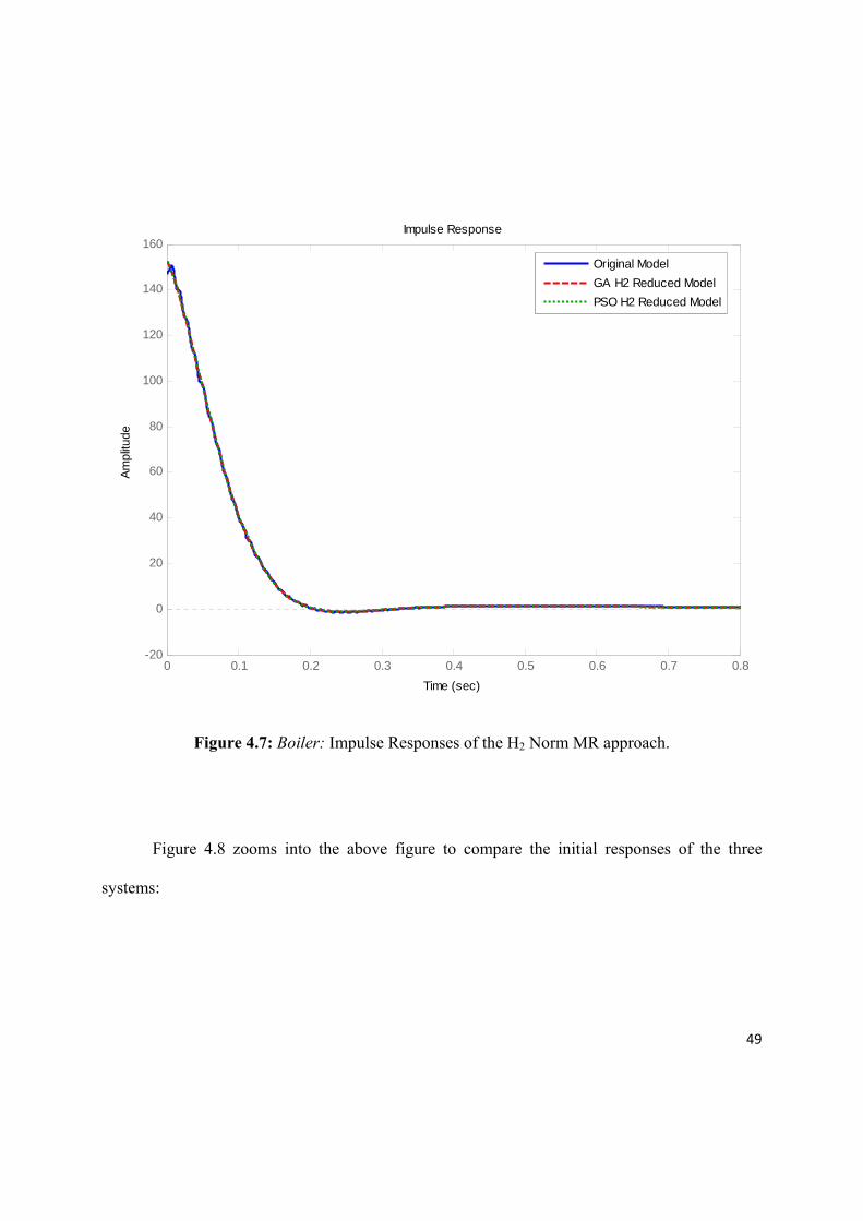
49

Figure 4.7: Boiler: Impulse Responses of the H2 Norm MR approach.

Figure 4.8 zooms into the above figure to compare the initial responses of the three

systems:

0 0.1 0.2 0.3 0.4 0.5 0.6 0.7 0.8-20

0

20

40

60

80

100

120

140

160Impulse Response

Time (sec)

Ampl

itude

Original ModelGA H2 Reduced ModelPSO H2 Reduced Model

50

Figure 4.8: Boiler: Initial Values of the H2 Norm MR approach.


original system. The initial values of the GA and PSO results are also relatively close to that of

the original system.

4.3.3 Step Responses:

Figure 4.9 compares the step responses of the original Wilson System to the result of

Wilson’s 2nd order Model Reduction approach of eq. (4.23) and the results of the GA and PSO

2nd order Model Reduction approaches:

0 0.002 0.004 0.006 0.008 0.01 0.012145

146

147

148

149

150

151

152

153Impulse Response

Time (sec)

Ampl

itude


51

Figure 4.9: Wilson: Step Responses of the H2 Norm MR approach.

Figure 4.10 compares the step responses of the original Boiler System to the results of the

GA and PSO 3rd order Model Reduction approaches:

0 1 2 3 4 5 6-0.005

0

0.005

0.01

0.015

0.02

0.025

0.03Step Response

Time (sec)

Ampl

itude


52

Figure 4.10: Boiler: Step Responses of the H2 Norm MR approach.

Note that the step responses of the reduced order models highly resemble those of the

original systems for both the Boiler and the Wilson example.

4.3.4 Frequency Responses:

Figure 4.11 compares the frequency responses of the original Wilson System to the result

of Wilson’s 2nd order Model Reduction approach and the results of the GA and PSO 2nd order

Model Reduction approaches:

0 0.5 1 1.5 2 2.5 3 3.5 4 4.5

Step Response

Time (sec)

Ampl

itude


53

Figure 4.11: Wilson: Frequency Responses of the H2 Norm MR approach.

Figure 4.12 compares the frequency responses of the original Boiler System to the results

of the GA and PSO 3rd order Model Reduction approaches:

-200

-150

-100

-50

0

Mag

nitu

de (d

B)

10-2

10-1

100

101

102

103

-180

-90

0

90

180

Phas

e (d

eg)

Bode Diagram

Frequency (rad/sec)

Original Wilson ModelReduced Wilson ModelH

2 GA Reduced Model

H2 PSO Reduced Model

54

Figure 4.12: Boiler: Frequency Responses of the H2 Norm MR approach.

Note that the frequency responses of the reduced order models highly resemble those of

the original systems at low frequencies. The magnitude of the reduced order models of the

Wilson example show some error at high frequencies due to the two missing states in the reduced

order models. The frequency responses of the reduced order Boiler models also tend to miss a

high frequency spark evident in the frequency response of the original Boiler system. However,

since most real-time physical systems operate at low frequencies, this error at high frequencies

tends to be acceptable and can be ignored.

-20

-10

0

10

20

30

Mag

nitu

de (d

B)

10-1

100

101

102

103

-135

-90

-45

0

Phas

e (d

eg)

Bode Diagram

Frequency (rad/sec)

Original ModelGA H2 Reduced Model

PSO H2 Reduced Model

55

4.4 GA and PSO H2 Norm Model Reduction Approachs vs. Previous Studies:

This section compares the norms of other researchers’ approaches to this studies proposed

approaches. Two papers (Maust & Feliachi, 1998) and (Yang, Hachino & Tsuji, 1996) used GA

to solve H2 Norm model reduction problems:

4.4.1 Maust and Feliachi:

Maust and Feliachi (1998) reduced the Wilson System of eq. (4.9) using Genetic

Algorithms. They used the H2 and L1 Norms of eq. (2.18) and eq. (2.19) respectively to perform

the model reduction, where the error was defined in eq. (1.9).

They set the fitness function to be maximized by the GA to be:

(4.24)

They used Genetic crossover (simple and arithmetic) and mutation operators to combine

information from candidate solutions to produce new solutions. Selection of next generation was

based on roulette-wheel.

Maust and Feliachi claim that their results were similar to that of Wilson (1970), with a

fitness value of 0.998, equivalent to a norm value of 2.004×10–3. Table 4.3 proves that the result

of this study’s proposed GA approach is better than that of Maust and Feliachi in terms of H2

Norms. Also, the PSO approach showed a better performance than the GA approach.

56

4.4.2 Yang, Hachino, and Tsuji:

Yang, Hachino, and Tsuji (1996) proposed a GA based H2 Norm model reduction

approach for SISO continuous time systems that introduces time delay into the reduced order

model.

Given an nth order SISO time delay system with transfer function:

exp (4.25)

where its rational part is stable and strictly proper, they tried to find a strictly proper lth order

reduced model with the time delay:

∏

exp

∏ .exp

(4.26)

Their cost function was defined as:

(4.27)

where W(jω) is a frequency weighting function introduced to obtain better approximation over a

pre-specified frequency range.

They used the following 6th order academic example from (Fukata, Mohri & Takata,

1983) and (Liu & Anderson, 1987) to test their approach:

57

.

(4.28)

Yang, Hachino and Tsuji reduced the above system into 1st order, 2nd order, 3rd order, and

4th order systems with time delay, and resulted with the following transfer functions respectively:

The 1st order reduced order model:

. ..

(4.29)

The 2nd order reduced order model:

. . . . .

(4.30)

The 3rd order reduced order model:

. . . . . . .

(4.31)

The 4th order reduced order model:

. . . . . . . . .

(4.32)

Using this study’s PSO approach to obtain the 1st order, 2nd order, 3rd order, and 4th order

reduced order models of system (4.30) with time delay resulted with the following systems

respectively:

The 1st order reduced order model:

. ..

(4.33)

58

The 2nd order reduced order model:

. . . .

(4.34)

The 3rd order reduced order model:

. . . . . . .

(4.35)

The 4th order reduced order model:

. . . . . . . . .

(4.36)

Table 4.5 compares the H2 Norms of the above eight reduced order models:

Table 4.5: H2 Norms of Yang’s 6th order example:

1st order 2nd order 3rd order 4th order

Yang’s GA Approach 1.0330×10–1 1.8286×10–2 1.3084×10–2 8.5880×10–3

Proposed PSO Approach 9.9326×10–2 1.8094×10–2 1.2937×10–2 8.2235×10–3

Table 4.5 proves that the proposed PSO approach yields better results than Yang et al.’s

proposed GA approach. Figures 4.13 to 4.24 show the impulse responses, step responses, and

frequency responses of the eight reduced order models in comparison to the original 6th order

system.

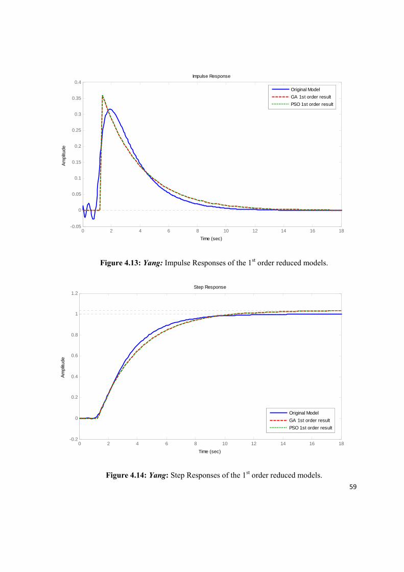
59

Figure 4.13: Yang: Impulse Responses of the 1st order reduced models.

Figure 4.14: Yang: Step Responses of the 1st order reduced models.

0 2 4 6 8 10 12 14 16 18-0.05

0

0.05

0.1

0.15

0.2

0.25

0.3

0.35

0.4Impulse Response

Time (sec)

Ampl

itude

Original ModelGA 1st order resultPSO 1st order result

0 2 4 6 8 10 12 14 16 18-0.2

0

0.2

0.4

0.6

0.8

1

1.2Step Response

Time (sec)

Ampl

itude

Original ModelGA 1st order resultPSO 1st order result

60

Figure 4.15: Yang: Frequency Responses of the 1st order reduced models.

Figure 4.16: Yang: Impulse Responses of the 2nd order reduced models.

-50

-40

-30

-20

-10

0

10

Mag

nitu

de (d

B)

10-2

10-1

100

101

-180

-90

0

90

180

Phas

e (d

eg)

Bode Diagram

Frequency (rad/sec)

Original Model

GA 1st order result

PSO 1st order result

0 2 4 6 8 10 12-0.05

0

0.05

0.1

0.15

0.2

0.25

0.3

0.35Impulse Response

Time (sec)

Ampl

itude

Original ModelGA 2nd order resultPSO 2nd order result

61

Figure 4.17: Yang: Step Responses of the 2nd order reduced models.

Figure 4.18: Yang: Frequency Responses of the 2nd order reduced models.

0 2 4 6 8 10 12-0.2

0

0.2

0.4

0.6

0.8

1

1.2Step Response

Time (sec)

Ampl

itude

Original ModelGA 2nd order resultPSO 2nd order result

-50

-40

-30

-20

-10

0

Mag

nitu

de (d

B)

10-2

10-1

100

101

-180

-90

0

90

180

Phas

e (d

eg)

Bode Diagram

Frequency (rad/sec)

Original Model

GA 2nd order result

PSO 2nd order result

62

Figure 4.19: Yang: Impulse Responses of the 3rd order reduced models.

Figure 4.20: Yang: Step Responses of the 3rd order reduced models.

0 1 2 3 4 5 6-0.05

0

0.05

0.1

0.15

0.2

0.25

0.3


Time (sec)

Ampl

itude

Original Model

GA 3rd order result

PSO 3rd order result

0 2 4 6 8 10 12-0.2

0

0.2

0.4

0.6

0.8

1

1.2Step Response

Time (sec)

Ampl

itude

Original Model

GA 3rd order result


63

Figure 4.21: Yang: Frequency Responses of the 3rd order reduced models.

Figure 4.22: Yang: Impulse Responses of the 4th order reduced models.

-50

-40

-30

-20

-10

0

10

Mag

nitu

de (d

B)

10-2

10-1

100

101

-180

-90

0

90

180

Phas

e (d

eg)

Bode Diagram

Frequency (rad/sec)

Original Model

GA 3rd order result


0 1 2 3 4 5 6 7 8 9 10-0.05

0

0.05

0.1

0.15

0.2

0.25

0.3


Time (sec)

Ampl

itude

Original ModelGA 4th order result

PSO 4th order result

64

Figure 4.23: Yang: Step Responses of the 4th order reduced models.

Figure 4.24: Yang: Frequency Responses of the 4th order reduced models.

0 2 4 6 8 10 12-0.2

0

0.2

0.4

0.6

0.8

1

1.2Step Response

Time (sec)

Ampl

itude

Original Model

GA 4th order result


-50

-40

-30

-20

-10

0

10

Mag

nitu

de (d

B)

10-2

10-1

100

101

-180

-90

0

90

180

Phas

e (d

eg)

Bode Diagram

Frequency (rad/sec)

Original Model

GA 4th order result


Chapter 5

H∞ Norm Model Reduction

onsider the general signal norm representation of eq.(4.1). Since we are studying

H∞ norm in this chapter, let p approach infinity (∞). Eq. (4.1) now becomes as

follows (Hartley et al., 1998):

lim | | (5.1)

For large p, the maximum values of y(t) are emphasized in the integral far more than the smaller

values; and therefore the integral becomes approximately proportional to the maximum value of

y(t) raised to the power p. Taking the pth root and letting p approach infinity yields the following

representation for the H∞ signal norm (Hartley et al., 1998):

sup | | (5.2)

C

66

Therefore, the H∞ norm of a signal is simply the magnitude of the largest value of the

signal . Moreover, the H∞ norm of a signal represents a bound on the signal amplitude for all

time. Unlike the L1 and the H2 norm, the H∞ norm of a signal may be finite even if the signal

does not decay (Hartley et al., 1998).

The H∞ norm of the system G(s) on the other hand is defined as (Doyle, Francis &

Tannenbaum, 1990):

sup | | (5.4)

Again, the H∞ norm of the system G(s) in the frequency domain is equal to the largest

magnitude of the frequency response over all frequencies. Graphically, it represents the highest

peak in the (Bode) magnitude plot of the transfer function, or the magnitude of the point on the

Nyquist plot farthest from the origin in the complex plane (Hartley et al., 1998).

The H∞ norm has a finite lower bound (Kavranoğlu & Bettayeb, 1993b). Consider the

Hankel singular values of the system G(s) defined in eq. (2.1). In H∞ Model Reduction, if the nth

order transfer function G(s) is reduced into an rth order transfer function Gr(s). Then:

(5.5)

where σr+1 is the (r + 1)st HSV of G(s).

For example, consider the Hankel singular values of the Wilson example given by eq.

(4.9) and its Hankel Singular Values of eq. (4.10). Since we are reducing the system into a 2nd

order model, then the largest dropped Hankel singular value is σ3 = 1.27×10–4. Therefore,

theoretically, the smallest achievable H∞ norm will be 1.27×10–4. Likewise, from the Hankel

67

singular values of the Boiler system given by eq. (4.12); we note the lower bound of H∞ norm in

3rd order model reduction will be 5.93×10–2.

However, it is convenient to mention here that those values are almost impossible to

achieve. But if one results with a close enough H∞ value, this would be a good indication that an

optimal solution was reached.

To compute the H∞ norm of a system G(s), consider the state space representation of that

system given by eq. (4.5). Define the 2n × 2n Hamiltonian matrix as follows (Doyle, Francis &

Tannenbaum, 1990):

(5.6)

As the theorem says; 1 if and only if H has no eigenvalues on the imaginary

axis (Doyle, Francis & Tannenbaum, 1990). Therefore, in order to compute the H∞ norm of the

system G(s), one should follow the following steps:

1. Select a positive number γ.

2. Test if γ (i.e. if γ 1) by calculating the eigenvalues of the resulting

Hamiltonian matrix.

3. Increase or decrease γ accordingly and repeat step 2.

It is also known that the H∞ norm of a system G(s) is always lower than the L1 norm of

that system (Hartley et al., 1998):

(5.7)

68

where g(t) is the impulse response of the system G(s). Therefore, if we perform L1 norm model

reduction, we are indirectly lowering the H∞ norm of the system error as well:

(5.8)

In the following sections, we will use the H∞ Norm Model Reduction approach to reduce

the 4th order Wilson system of eq. (4.9) into a 2nd order reduced model, and the 9th order Boiler

system of eq. (4.11) into a 3rd order reduced model. The H∞ Norm fitness function that was

implemented in MATLAB computes the peak gain of the frequency response (the magnitude of

the maximum point in the Bode plot) of the error between the original system and the reduced

order model with the same stability constraint explained in Chapter 4.


The same GA settings as in eq. (4.13) were used to perform the model reduction for both

the Wilson System and the Boiler system in this chapter.

The following system represents the 2nd order result of the H∞ Norm Model Reduction


3.457 6.0490.3239 0.2429 0.2793

0.01254

0.05126 1.428

(5.9)



69

The following system on the other hand represents the 3rd order result of the H∞ Norm


6.449 29.73 0.38563.129 21.71 10.694.918 6.326 6.661

4.9214.127

10.74

6.591 0.1677 10.71

(5.10)




At first, we used the same settings of eq. (4.18) to reduce the Wilson system and the

Boiler system. But unfortunately, our PSO kept getting stuck at some local minima. We wanted

to study the effect of the maximum velocity of a particle (mv) and started by increasing it to 10,

50 and 100. We noted that increasing mv makes the fitness value drop faster at first. However, it

dropped very fast but never converged. Lower mv might be slower, but it guarantees that the

PSO never misses the solution by jumping over it. However decreasing mv too much limits the

search space, and thus does not help the PSO to converge.

Different mv values were tried step by step (3.5, 3, 2.5, 2, 1.5 and 1) and the value 2 made

the PSO converge for the Boiler system. The next step was decreasing and increasing c1 and c2

but that did not improve the PSO’s performance for the Wilson system. We then started

increasing and decreasing different parameters, trying different combinations until mv = 2 and

epoch when inertial weight at final value = 20,000 converged to a solution.

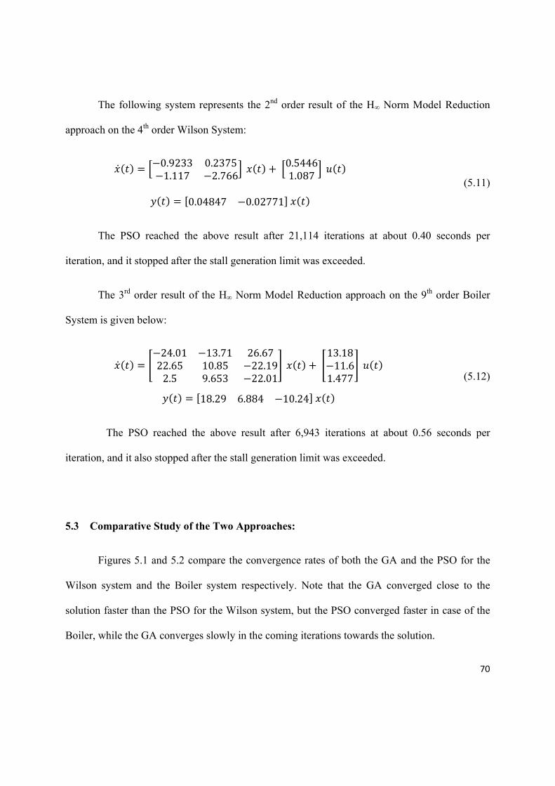
70

The following system represents the 2nd order result of the H∞ Norm Model Reduction


0.9233 0.23751.117 2.766 0.5446

1.087

0.04847 0.02771

(5.11)



The 3rd order result of the H∞ Norm Model Reduction approach on the 9th order Boiler


24.01 13.71 26.6722.65 10.85 22.19

2.5 9.653 22.01

13.1811.6

1.477

18.29 6.884 10.24

(5.12)





Wilson system and the Boiler system respectively. Note that the GA converged close to the

solution faster than the PSO for the Wilson system, but the PSO converged faster in case of the

Boiler, while the GA converges slowly in the coming iterations towards the solution.

71



0 50 100 150 200 250 300 350 400 450 50010-4

10-3

10-2

10-1

100

Generations

Gbe

st

Hoo Model Reduction of Wilson System


0 500 1000 1500 2000 2500 3000 3500 400010-1

100

101

102Hoo Model Reduction of Boiler System

Gbe

st

Generations


72

The following sections will compare Wilson’s result of eq. (4.23) to the results of the GA

and the PSO approaches, as well as comparing the GA results of the Boiler system model

reduction to those of the PSO.




Table 5.1: Wilson: SSE and Norms of the H∞ Norm MR approach:


Wilson’s Result 9.324×10–5 6.724×10–4 2.525×10–4 6.957×10–4

GA Approach 2.144×10–6 6.601×10–4 2.239×10–4 7.818×10–4

PSO Approach 2.144×10–4 6.593×10–4 2.144×10–4 8.123×10–4

Table 5.2: Boiler: SSE and Norms of the H∞ Norm MR approach:


GA Approach 1.126×10–1 6.844×10–1 1.127×10–1 3.154×10–1

PSO Approach 1.275×10–3 6.917×10–1 1.116×10–1 3.137×10–1

73



Wilson’s 2nd order Model Reduction approach and the results of the GA and PSO 2nd order


Figure 5.3: Wilson: Impulse Responses of the H∞ Norm MR approach.


different systems:

0 1 2 3 4 5 6-4

-2

0

2

4

6

8

10

12

14

16x 10

-3 Impulse Response

Time (sec)

Ampl

itude


inf2 GA Reduced Model

Hinf

PSO Reduced Model

74

Figure 5.4: Wilson: Initial Values of the H∞ Norm MR approach.


original system. The three reduced order models are also close to the original system in terms of

initial values with a small error of about 3.65×10–3.



0 0.01 0.02 0.03 0.04 0.05 0.06 0.07 0.08

-4

-3

-2

-1

0

1

2x 10

-3 Impulse Response

Time (sec)

Ampl

itude


inf2 GA Reduced Model

Hinf

PSO Reduced Model

75

Figure 5.5: Boiler: Impulse Responses of the H∞ Norm MR approach.


systems:

0 0.1 0.2 0.3 0.4 0.5 0.6 0.7-20

0

20

40

60

80

100

120

140

160Impulse Response

Time (sec)

Ampl

itude

Original ModelGA H

inf Reduced Model

PSO Hinf

Reduced Model

76

Figure 5.6: Boiler: Initial Values of the H∞ Norm MR approach.


original system, and their initial values are also relatively close to that of the original system.





0 0.005 0.01 0.015142

143

144

145

146

147

148

149

150

151

152Impulse Response

Time (sec)

Ampl

itude

Original ModelGA Hinf Reduced Model

PSO Hinf Reduced Model

77

Figure 5.7: Wilson: Step Responses of the H∞ Norm MR approach.



0 1 2 3 4 5 6-0.005

0

0.005

0.01

0.015

0.02

0.025

0.03Step Response

Time (sec)

Ampl

itude

Original Wilson Model

Reduced Wilson Model

Hinf

GA Reduced Model

Hinf PSO Reduced Model

78

Figure 5.8: Boiler: Step Responses of the H∞ Norm MR approach.

The step responses of the reduced order Wilson and Boiler models also highly resemble

those of the original systems.





0 0.5 1 1.5 2 2.5 3 3.5 4 4.5 50

2

4

6

8

10

12

14Step Response

Time (sec)

Ampl

itude

Original Model

GA Hinf

Reduced Model

PSO Hinf

Reduced Model

79

Figure 5.9: Wilson: Frequency Responses of the H∞ Norm MR approach.



-200

-150

-100

-50

0

Mag

nitu

de (d

B)

10-2

10-1

100

101

102

103

-180

-90

0

90

180

Phas

e (d

eg)

Bode Diagram

Frequency (rad/sec)

Original Wilson ModelReduced Wilson ModelHoo GA Reduced Model

Hoo PSO Reduced Model

80

Figure 5.10: Boiler: Frequency Responses of the H∞ Norm MR approach.

Note that the frequency response behavior of the H∞ reduced order models is similar to

those of the H2 Norm reduced order models at high frequencies. However, since most real-time

physical systems operate at low frequencies, this error at high frequencies can be ignored.

5.4 PSO H∞ Norm Model Reduction Approach vs. Previous Studies:

Tan and Li (1996) investigated weighted H∞ Model Reduction using Genetic Algorithms.

Given an mth order transfer function G(s), they find a reduced model Gr(s) such that the cost

function JG is minimized given a frequency weighting function Wα(s):

-20

-10

0

10

20

30

Mag

nitu

de (d

B)

10-1

100

101

102

103

-135

-90

-45

0

Phas

e (d

eg)

Bode Diagram

Frequency (rad/sec)

Original ModelGA Hoo Reduced Model

PSO Hoo Reduced Model

81

(5.13)

Another objective of their work was to find an optimal W(s) such that the cost function:

(5.14)

is minimized under the constraint:

1 (5.15)

where Wβ(s) is also a frequency weighting function.

Minimizing both JG and JW for an infinite number of frequency points is impossible.

However, minimizing an approximate JG and JW over a certain range of interest is possible and is

adopted in practice.

To improve the GA performance, the “generational” optimization power of crossover of

an evolving population is combined with the Lamarckism “inheritance”. A Boltzmann type of

learning is realized by simulated annealing (SA) which asserts a probability of retaining possible

search directions.

An existing chromosome Ck will mutate to chromosome C with a probability:

| min exp , 1 (5.16)

where kB is set to 5×10–5, the annealing temperature T decreases from Tini exponentially at a rate

of βj–1 where β < 1 is the annealing factor and the integer 1, is the annealing cycle.

82

The final temperature Tfinal is determined by how tight the fine tuning should be bounded at the

end of the learning process. They set β = 30%, Tini = 105, Tfinal = 1, and jmax = 10.

50% of the wining chromosomes will be trained for Lamarkian heredity. The new

population will contain winning individuals and 25% of the parents.

Chen and Li used the following 4th order example to test their GA H∞ Model Reduction

approach:

. . . .

. . . .

(5.17)

with the following frequency weighing function:

.

(5.18)

They reduced the above example into a 2nd order model using the norm of eq. (5.13) and

they resulted with the following reduced order model:

. . . . .

(5.19)

Using the same frequency weighing function of eq. (5.18) and the weighted H∞ norm of

eq. (5.13), we used PSO to find a 2nd order reduced model for the 4th order example of eq. (5.17)

and resulted with the following reduced order model:

. . . . .

(5.20)

Table 5.3 below compares our result to the results of previous researches:

83

Table 5.3: Weighted H∞ Norm Model Reduction Results:

Model Reduction Approach 2nd order

Lower Bound ( Hankel Singular Value) 2.704

Latham & Anderson (1986) 20.08

Chiang & Safonov (1992) 11.71

Zhou (1995) (Algorithm I) 4.827

Zhou (1995) (Algorithm II) 4.822

Al-Amer (1998) 4.629

Tan & Li (1996): GA Approach 4.517

PSO Approach 4.4899

Note that our PSO results outperformed all previous results in the sense of the weighted

H∞ norm of the error between the original model and the reduced order model.

Chapter 6

L1 Norm Model Reduction

onsider the general signal norm representation of eq.(4.1). Since we are studying

the L1 norm in this chapter, we set p in the equation to 1. The L1 norm of the

signal y(t) becomes as follows (Hartley et al., 1998):

| | (6.1)

The L1 norm of the system with transfer function G(s) and impulse response g(t) on the

other hand is defined as (Doyle, Francis & Tannenbaum, 1990):

| |∞ (6.2)

In the following sections, we will use the L1 Norm Model Reduction approach to reduce

the 4th order Wilson system of eq. (4.9) into a 2nd order reduced model, and the 9th order Boiler

system of eq. (4.11) into a 3rd order reduced model. The L1 Norm fitness function of eq. (1.8)

C

85

was implemented in MATLAB using trapezoidal numerical integration which computes an

approximate integral of the error between the impulse response of the original system and the

impulse response of the reduced order system with respect to time with the same stability

constraint explained in Chapter 4.


The same GA settings as in eq. (4.13) were used to perform the model reduction for both

the Wilson System and the Boiler System in this chapter.

The following system represents the 2nd order result of the L1 Norm Model Reduction


0.4424 0.5342.786 3.64 0.153

0.2807

0.08699 0.06831

(6.3)



The following system on the other hand represents the 3rd order result of the L1 Norm


11.09 4.571 9.02613.88 12.67 0.41652.227 10.96 7.111

11.717.382.852

15.31 3.912 1.684

(6.4)

86




At first, we used the same settings of eq. (4.18) to reduce the Wilson system and the

Boiler system. The PSO converged for the Boiler but got stuck at some local minima while

reducing the Wilson system. We tried decreasing and increasing the maximum velocity of a

particle (mv) but with no success. Finally, we increased the epoch when inertial weight at final

value step by step until the value 10,000 converged to a solution.

The following system represents the 2nd order result of the L1 Norm Model Reduction


2.563 0.44361.914 1.55 0.162

0.0913

0.2252 0.4653

(6.5)



The 3rd order result of the L1 Norm Model Reduction approach on the 9th order Boiler


87

22.39 15.4 36.727.205 11.16 8.467

2.617 3.022 2.375

14.7715.326.453

7.173 1.743 11.6

(6.6)





Wilson system and the Boiler system respectively. Note that in both cases, the GA converges

faster towards the solution than does the PSO.


0 50 100 150 200 250 300 350 400 450 50010-4

10-3

10-2

10-1

100

101

Generations

Gbe

st

L1 Model Reduction of Wilson System


88


The following sections will compare Wilson’s result of eq.(4.23) to the results of the GA

and the PSO approaches, as well as comparing the GA results of the Boiler system model

reduction to those of the PSO.




0 500 1000 1500 2000 2500 3000 3500 4000 4500 500010

-1

100

101

102

L1 Model Reduction of Boiler System

Generations

Gbe

st


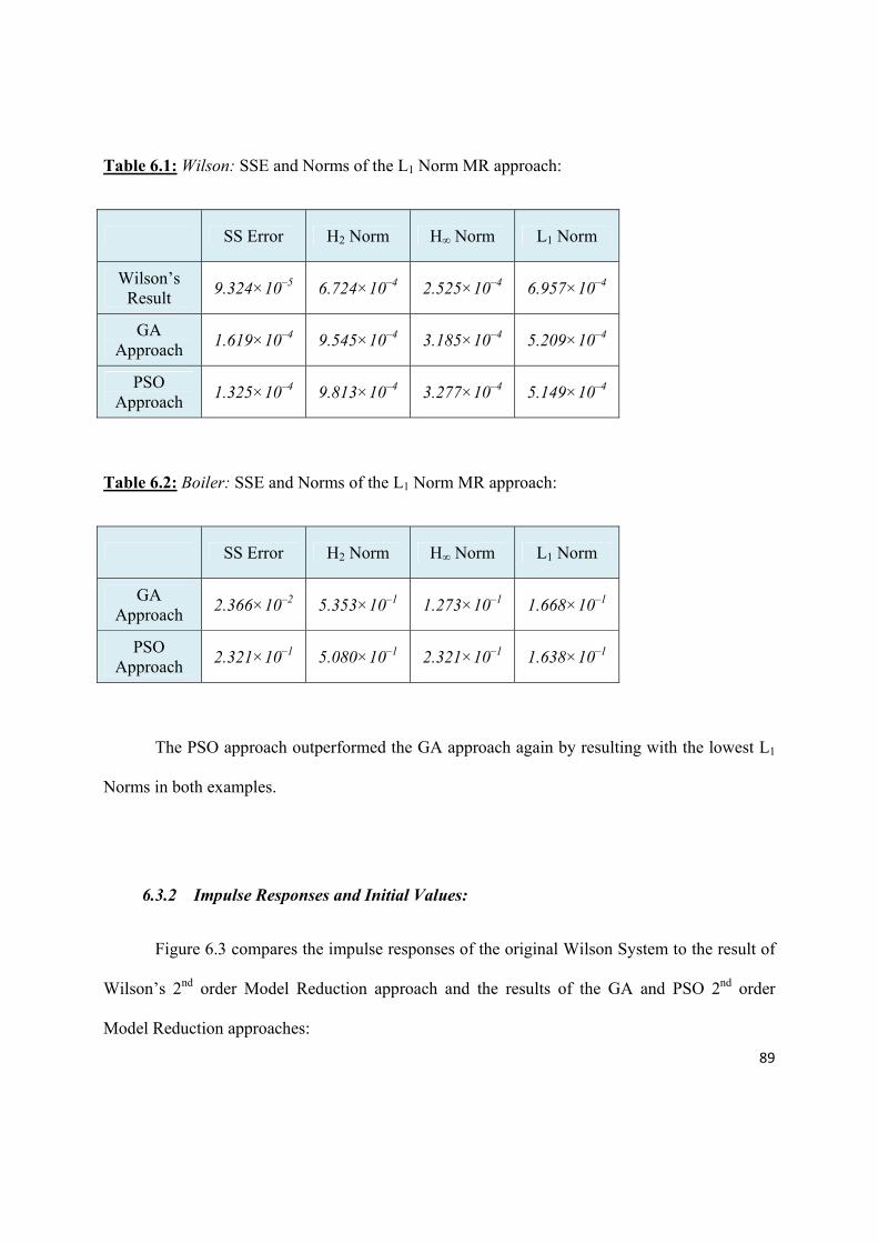
89

Table 6.1: Wilson: SSE and Norms of the L1 Norm MR approach:


Wilson’s Result 9.324×10–5 6.724×10–4 2.525×10–4 6.957×10–4

GA Approach 1.619×10–4 9.545×10–4 3.185×10–4 5.209×10–4

PSO Approach 1.325×10–4 9.813×10–4 3.277×10–4 5.149×10–4

Table 6.2: Boiler: SSE and Norms of the L1 Norm MR approach:


GA Approach 2.366×10–2 5.353×10–1 1.273×10–1 1.668×10–1

PSO Approach 2.321×10–1 5.080×10–1 2.321×10–1 1.638×10–1

The PSO approach outperformed the GA approach again by resulting with the lowest L1

Norms in both examples.





90

Figure 6.3: Wilson: Impulse Responses of the L1 Norm MR approach.


different systems:

0 1 2 3 4 5 6-0.01

-0.005

0

0.005

0.01

0.015


Time (sec)

Ampl

itude

Original Wilson ModelReduced Wilson ModelL1 GA Reduced ModelL1 PSO Reduced Model

91

Figure 6.4: Wilson: Initial Values of the L1 Norm MR approach.



0 0.01 0.02 0.03 0.04 0.05 0.06 0.07 0.08 0.09 0.1

-6

-5

-4

-3

-2

-1

0

1

2x 10

-3 Impulse Response

Time (sec)

Ampl

itude


92

Figure 6.5: Boiler: Impulse Responses of the L1 Norm MR approach.


systems:

0 0.1 0.2 0.3 0.4 0.5 0.6 0.7 0.8 0.9-20

0

20

40

60

80

100

120

140

160Impulse Response

Time (sec)

Ampl

itude

Original ModelGA L1 Reduced ModelPSO L1 Reduced Model

93

Figure 6.6: Boiler: Initial Values of the L1 Norm MR approach.

Note that the impulse responses of the reduced order Boiler and Wilson models highly

resemble those of the original systems, and their initial values are also relatively close to those of

the original systems.





0 0.002 0.004 0.006 0.008 0.01 0.012145

146

147

148

149

150

151

152

153

154

155

156Impulse Response

Time (sec)

Ampl

itude


94

Figure 6.7: Wilson: Step Responses of the L1 Norm MR approach.



0 1 2 3 4 5 6-0.005

0

0.005

0.01

0.015

0.02

0.025

0.03Step Response

Time (sec)

Ampl

itude


95

Figure 6.8: Boiler: Step Responses of the L1 Norm MR approach.

It can be noted from figures 6.7 and 6.8 that the step responses of the reduced order

Wilson and Boiler models highly resemble those of the original system.





0 0.5 1 1.5 2 2.5 3 3.5 4 4.5 50

2

4

6

8

10

12

14Step Response

Time (sec)

Ampl

itude


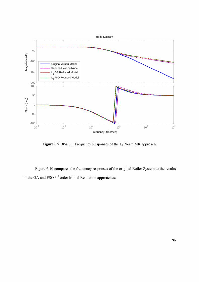
96

Figure 6.9: Wilson: Frequency Responses of the L1 Norm MR approach.



-200

-150

-100

-50

0

Mag

nitu

de (d

B)

10-2

10-1

100

101

102

103

-180

-90

0

90

180

Phas

e (d

eg)

Bode Diagram

Frequency (rad/sec)

Original Wilson ModelReduced Wilson ModelL1 GA Reduced Model

L1 PSO Reduced Model

97

Figure 6.10: Boiler: Frequency Responses of the L1 Norm MR approach.

Note that the frequency response behavior of the L1 reduced order models is similar to

those of the reduced order models in previous chapters at high frequencies. However, since most

real-time physical systems operate at low frequencies, the high frequency error can be ignored.

6.4 GA and PSO L1 Norm Model Reduction Approaches vs. Previous Studies:

As stated before in section 4.4.1, Maust and Feliachi (1998) reduced the Wilson System of

eq. (4.9) using Genetic Algorithms and both H2 and L1 Norms. They claim that the L1 Norm

-20

-10

0

10

20

30

Mag

nitu

de (d

B)

10-1

100

101

102

103

-135

-90

-45

0

Phas

e (d

eg)

Bode Diagram

Frequency (rad/sec)

Original ModelGA L

1 Reduced Model

PSO L1 Reduced Model

98

model reduction result they achieved was similar to that achieved by Wilson (1970) with a

2.004×10–3 norm value. Table 6.1 illustrates that the result of this study’s proposed GA approach

is better than that of Maust and Feliachi in terms of L1 Norms, and the PSO results of Table 6.1

obviously outperform those of the GA.

Chapter 7

Hybrid Norm Model Reduction

he use of different norms gives rise to different approximations since different

norms favors different time-domain or frequency-domain characteristics of the

system. However, it is sometimes desirable to obtain a reduced order model with certain

desirable characteristics that might not be achievable by the use of a single norm. Therefore, we

propose the following hybrid norm criterion to obtain better compromised reduced order models:

The Hybrid Norm was defined as follows:

(7.1)

We use two different Hybrid Norm Model Reduction approaches to reduce the 4th order

Wilson system of eq. (4.9) and the 9th order Boiler system of eq. (4.11).

T

100

7.1 Hybrid between H2 and H∞ Norms:

The first Hybrid Norm used was between H2 and H∞ Norms where α = β = 1, and γ = 0.

7.1.1 GA Approach Results:

The same GA settings as in eq.(4.13) were used to perform the model reduction for both

the Wilson System and the Boiler system in this section.

The following system represents the 2nd order result of the first Hybrid Norm Model

Reduction approach on the 4th order Wilson System:

1.029 0.029860.7105 2.741 0.5345

0.3102

0.3347 0.5891

(7.2)



The following system on the other hand represents the 3rd order result of the first Hybrid

Norm Model Reduction approach on the 9th order Boiler System:

6.011 5.836 4.0558.45 10.8 5.94412.52 17 15.5

10.27

3.8359.24

3.857 3.153 10.87

(7.3)



101

7.1.2 PSO Approach Results:

The PSO settings used to perform the model reduction for both the Wilson and Boiler

Systems were similar to those of eq. (4.18) except the maximum velocity of a particle was set to

3, and the epoch when inertial weight at final value was set to 10,000.

The following system represents the 2nd order result of the first Hybrid Norm Model


3.652 2.7931 0 1

0

0.003516 0.07387

(7.4)



The 3rd order result of the first Hybrid Norm Model Reduction approach on the 9th order

Boiler System is given below:

5.051 8.524 0.703626.56 20.56 13.4915.59 2.529 16.91

1.859

7.8884.772

20.02 3.646 33.64

(7.5)



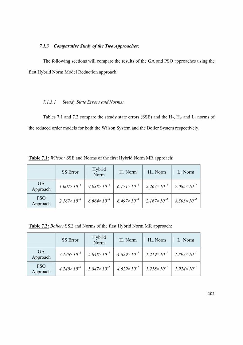
102

7.1.3 Comparative Study of the Two Approaches:

The following sections will compare the results of the GA and PSO approaches using the

first Hybrid Norm Model Reduction approach:

7.1.3.1 Steady State Errors and Norms:



Table 7.1: Wilson: SSE and Norms of the first Hybrid Norm MR approach:

SS Error Hybrid Norm H2 Norm H∞ Norm L1 Norm

GA Approach 1.007×10–4 9.038×10–4 6.771×10–4 2.267×10–4 7.085×10–4

PSO Approach 2.167×10–4 8.664×10–4 6.497×10–4 2.167×10–4 8.503×10–4

Table 7.2: Boiler: SSE and Norms of the first Hybrid Norm MR approach:


GA Approach 7.126×10–3 5.848×10–1 4.629×10–1 1.219×10–1 1.893×10–1

PSO Approach 4.240×10–3 5.847×10–1 4.629×10–1 1.218×10–1 1.924×10–1

103

7.1.3.2 Impulse Responses and Initial Values:

Figure 7.1 compares the impulse responses of the original Wilson System to the results of

the GA and PSO 2nd order Model Reduction approaches:

Figure 7.1: Wilson: Impulse Responses of the first Hybrid Norm MR approach.


different systems:

0 1 2 3 4 5 6-4

-2

0

2

4

6

8

10

12

14

16x 10

-3 Impulse Response

Time (sec)

Ampl

itude

Original Wilson ModelReduced Wilson ModelHybrid

1 GA Reduced Model

Hybrid1 PSO Reduced Model

104

Figure 7.2: Wilson: Initial Values of the first Hybrid Norm MR approach.



0 0.01 0.02 0.03 0.04 0.05 0.06 0.07 0.08

-4

-3

-2

-1

0

1

2x 10

-3 Impulse Response

Time (sec)

Ampl

itude


1 GA Reduced Model


105

Figure 7.3: Boiler: Impulse Responses of the first Hybrid Norm MR approach.


systems:

0 0.1 0.2 0.3 0.4 0.5 0.6 0.7 0.8-20

0

20

40

60

80

100

120

140

160Impulse Response

Time (sec)

Ampl

itude

Original ModelGA Hybrid

1 Reduced Model

PSO Hybrid1 Reduced Model

106

Figure 7.4: Boiler: Initial Values of the first Hybrid Norm MR approach.

7.1.3.3 Step Responses:

Figure 7.5 compares the step responses of the original Wilson System to the results of the

GA and PSO 2nd order Model Reduction approaches:

0 0.002 0.004 0.006 0.008 0.01 0.012145

146

147

148

149

150

151

152

153Impulse Response

Time (sec)

Ampl

itude


1 Reduced Model


107

Figure 7.5: Wilson: Step Responses of the first Hybrid Norm MR approach.



0 1 2 3 4 5 6-0.005

0

0.005

0.01

0.015

0.02

0.025

0.03Step Response

Time (sec)

Ampl

itude


1 GA Reduced Model


108

Figure 7.6: Boiler: Step Responses of the first Hybrid Norm MR approach.

7.1.3.4 Frequency Responses:

Figure 7.7 compares the frequency responses of the original Wilson System to the results

of the GA and PSO 2nd order Model Reduction approaches:

0 0.5 1 1.5 2 2.5 3 3.5 4 4.50

2

4

6

8

10

12

14Step Response

Time (sec)

Ampl

itude


1 Reduced Model


109

Figure 7.7: Wilson: Frequency Responses of the first Hybrid Norm MR approach.



-200

-150

-100

-50

0

Mag

nitu

de (d

B)

10-2

10-1

100

101

102

103

-180

-90

0

90

180

Phas

e (d

eg)

Bode Diagram

Frequency (rad/sec)

Original Wilson ModelReduced Wilson ModelHybrid1 GA Reduced Model


110

Figure 7.8: Boiler: Frequency Responses of the first Hybrid Norm MR approach.

Note that the impulse responses, initial values and step responses of all reduced order

models highly resemble those of the original systems. Also, the frequency response behavior of

the reduced order models closely resembles those of the original systems with some error at high

frequencies that can be ignored.

7.2 Hybrid between H2, H∞ and L1 Norms:

The second Hybrid Norm used was between H2, H∞ and L1 Norms where α = β = γ = 1.

-20

-10

0

10

20

30

Mag

nitu

de (d

B)

10-1

100

101

102

103

-135

-90

-45

0

Phas

e (d

eg)

Bode Diagram

Frequency (rad/sec)

Original ModelGA Hybrid1 Reduced Model


111

7.2.1 GA Approach Results:

The same GA settings as in eq.(4.13) were used to perform the model reduction for both

the Wilson System and the Boiler system in this section.

The following system represents the 2nd order result of the second Hybrid Norm Model


1.121 0.04663.752 2.813 0.02225

0.007088

0.6188 1.292

(7.6)



The following system on the other hand represents the 3rd order result of the second

Hybrid Norm Model Reduction approach on the 9th order Boiler System:

3.386 5.843 7.6482.665 9.198 22.013.953 5.894 18.95

4.9977.693

7.099

2.8 11.64 6.937

(7.7)



112

7.2.2 PSO Approach Results:

The PSO settings used to perform the model reduction for both the Wilson and Boiler

Systems were similar to those of eq. (4.18) except the maximum velocity of a particle was set to

3, and the Epoch when inertial weight at final value was set to 10,000.

The following system represents the 2nd order result of the second Hybrid Norm Model


3.852 2.9061 0 1

0

0.004068 0.07726

(7.8)



The 3rd order result of the second Hybrid Norm Model Reduction approach on the 9th

order Boiler System is given below:

8.64 10.06 6.5065.201 0.4313 4.56733.39 5.159 23.5

1.0883.49117.47

18.73 17.98 11.16

(7.9)



113

7.2.3 Comparative Study of the Two Approaches:

The following sections will compare the results of the GA and PSO approaches using the

second Hybrid Norm Model Reduction approach:

7.2.3.1 Steady State Errors and Norms:



Table 7.3: Wilson: SSE and Norms of the second Hybrid Norm MR approach:


GA Approach

7.976×10–5 1.615×10–3 7.614×10–4 2.584×10–4 5.947×10–4

PSO Approach

8.432×10–5 1.586×10–3 7.027×10–4 2.425×10–4 6.412×10–4

Table 7.4: Boiler: SSE and Norms of the second Hybrid Norm MR approach:


GA Approach 8.715×10–3 7.652×10–1 4.726×10–1 1.231×10–1 1.695×10–1

PSO Approach 2.489×10–2 7.643×10–1 4.691×10–1 1.227×10–1 1.725×10–1

114

7.2.3.2 Impulse Responses and Initial Values:

Figure 7.9 compares the impulse responses of the original Wilson System to the results of


Figure 7.9: Wilson: Impulse Responses of the second Hybrid Norm MR approach.


different systems:

0 1 2 3 4 5 6-5

0

5

10

15

20x 10

-3 Impulse Response

Time (sec)

Ampl

itude



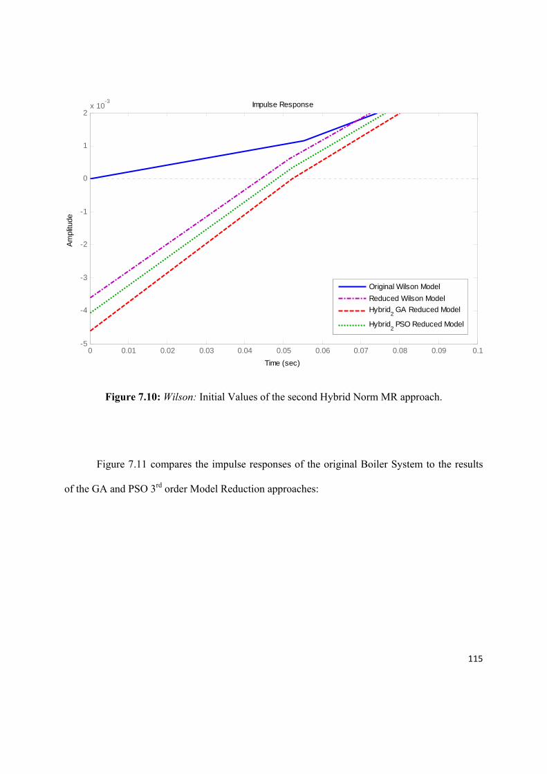
115

Figure 7.10: Wilson: Initial Values of the second Hybrid Norm MR approach.

Figure 7.11 compares the impulse responses of the original Boiler System to the results


0 0.01 0.02 0.03 0.04 0.05 0.06 0.07 0.08 0.09 0.1-5

-4

-3

-2

-1

0

1

2x 10

-3 Impulse Response

Time (sec)

Ampl

itude



116

Figure 7.11: Boiler: Impulse Responses of the second Hybrid Norm MR approach.


systems:

0 0.1 0.2 0.3 0.4 0.5 0.6 0.7 0.8-20

0

20

40

60

80

100

120

140

160Impulse Response

Time (sec)

Ampl

itude



117

Figure 7.12: Boiler: Initial Values of the second Hybrid Norm MR approach.

7.2.3.3 Step Responses:

Figure 7.13 compares the step responses of the original Wilson System to the results of


0 0.002 0.004 0.006 0.008 0.01 0.012145

146

147

148

149

150

151

152

153Impulse Response

Time (sec)

Ampl

itude


2 Reduced Model


118

Figure 7.13: Wilson: Step Responses of the second Hybrid Norm MR approach.



0 1 2 3 4 5 6-0.005

0

0.005

0.01

0.015

0.02

0.025

0.03Step Response

Time (sec)

Ampl

itude



119

Figure 7.14: Boiler: Step Responses of the second Hybrid Norm MR approach.

7.2.3.4 Frequency Responses:

Figure 7.15 compares the frequency responses of the original Wilson System to the

results of the GA and PSO 2nd order Model Reduction approaches:

0 0.5 1 1.5 2 2.5 3 3.5 4 4.50

2

4

6

8

10

12

14Step Response

Time (sec)

Ampl

itude


2 Reduced Model


120

Figure 7.15: Wilson: Frequency Responses of the second Hybrid Norm MR approach.



-200

-150

-100

-50

0

Mag

nitu

de (d

B)

10-2

10-1

100

101

102

103

-180

-90

0

90

180

Phas

e (d

eg)

Bode Diagram

Frequency (rad/sec)


2 GA Reduced Model


121

Figure 7.16: Boiler: Frequency Responses of the second Hybrid Norm MR approach.

The impulse responses, initial values and step responses of all reduced order models

highly resemble those of the original systems. The frequency response behavior of the reduced

order models also closely resembles those of the original systems with some ignorable error at

high frequencies.

7.3 Comparison between the Two Hybrid Norms:

The use of hybrid norm results with a compromised reduced order model that is low in

two or three different norms. The first hybrid norm worked at obtaining a reduced order model

-20

-10

0

10

20

30

Mag

nitu

de (d

B)

10-1

100

101

102

103

-135

-90

-45

0

Phas

e (d

eg)

Bode Diagram

Frequency (rad/sec)



122

with low H2 and H∞ norms, while the second hybrid norm worked at obtaining a reduced order

model that is law in all three norms (H2, H∞ and L1).

However, since the model reduction was based on different norms that favor different

characteristics of the system, each individual norm in the hybrid norm result was not as good as

the norm achieved using that norm’s reduction alone. For example, the H2 norms of the hybrid

norm reduced order models are not as good as the H2 norm achieved by H2 norm model

reduction. However, the hybrid norm, results with a better combination between all norms of

concern.

Similarly, note that the results of the first hybrid norm have a good H2–H∞ combination

but with relatively high L1 norms. The second hybrid norm takes the L1 norm into consideration,

and therefore does not do as well as the first hybrid norm for both H2 and H∞ norms, but rather

results with a better combination between all three norms.

It is also obvious that the PSO tends to perform better that the GA by resulting with lower

hybrid norm for all the presented examples.

Chapter 8

Conclusion & Future Work

odern engineering systems such as telecommunication systems, transmission

lines, and chemical reactors are complex in nature. Their detailed mathematical

modeling leads to high order dynamic systems.

For simplicity of simulation, interpretation, and control of such processes it is desirable to

represent the dynamics of these high order systems by lower order models. However, most of the

available optimal model reduction techniques follow computationally demanding, time

consuming, iterative procedures that usually result in non-robustly stable models with poor

frequency response resemblance to the original high order model in some frequency ranges.

Genetic Algorithms (GA) and Particle Swarm Optimization (PSO) are two of the most

powerful optimization tools. They were used to find optimum reduced models for two complex

high order SISO models using H2 Norm, H∞ Norm, L1 Norm, and two different Hybrid Norms.

M

124

The use of GA and PSO in Model reduction helped simplify and automate the model reduction

process. They help one avoid tedious iterative mathematical time consuming procedures (leading

often to local optimum solutions) while obtaining very satisfying results.

GAs and PSO helps us obtain solutions to problems for which analytical solutions are not

available and for which classical optimization techniques can give at best local solutions that are

sensitive to initial guesses.

However, it is convenient to mention here that although optimal model reduction using

Genetic Algorithms and Particle Swarm Optimization seem very attractive; they suffer from one

major drawback.

There is no systematic way in theory to find the appropriate settings of either the GA or

the PSO for a certain application. In fact, trial and error is the only method used by all

researchers in the area of those two evolutionary algorithms. And thus, finding the correct

appropriate settings to work your application could be time consuming.

The settings used for the GA however, worked for all the model reduction examples we

tried with different orders, while the PSO gave us a hard time to find the right settings for each

example.

Moreover, if you try to reduce a different system using PSO, the same set of settings used

in this thesis might not work. In fact, if certain set of settings work for a certain system in H2

Norm Model Reduction for example; they might not work for H∞, L1, or Hybrid Norm Model

Reduction of the same system.

125

Therefore one should start with the default settings of the PSO, and if they do not work;

one shall start altering the rest of the parameters one by one, and try to draw a conclusion on the

effect of certain parameters on reducing the given system, and then decrease or increase the

parameters accordingly.

The population size of the GA and the swarm size of the PSO do not affect their

probability of convergence to a solution. However, we noted that GA converges faster to the

solution than does the PSO in almost all cases.

Decreasing the inertial weights at the final iterations in the PSO, decreases the effect of

the particles’ velocity whilst increasing the effect of the particles’ best achieved fitness value and

the global best achieved fitness value of the swarm, and therefore helps fine tune the result at the

final iterations.

Increasing the maximum particle velocity in the PSO, increases the convergence speed of

the PSO. However, a very high maximum particle velocity value might cause the PSO to miss the

solution and get trapped in local minima. On the other hand, a too small maximum particle

velocity value limits the search space of the PSO.

Comparing the GA results to the PSO results; it was found that PSO outperformed the

GA in the norm sense by leading to better (lower) norms. Also, it is noted that the simplicity of

the computations in the PSO Algorithm in comparison to the GA Algorithm makes it much faster

time-wise, but the GA tends to converge faster close to the solution iteration-wise. Therefore we

can conclude that PSO has the same effectiveness as GA in finding the global optimal solution

but with significantly better computational efficiency (Hassan et al., 2005).

126

Tables 8.1 and 8.2 summarize the results of this thesis study:

Table 8.1: Summary of the Wilson System Results:


H2 model reduction

GA 9.780×10–5 6.556×10–4 2.729×10–4 7.759×10–4

PSO 1.968×10–4 6.450×10–4 2.405×10–4 8.678×10–4

H∞ model reduction

GA 2.144×10–6 6.601×10–4 2.239×10–4 7.818×10–4

PSO 2.144×10–4 6.593×10–4 2.144×10–4 8.123×10–4

L1 model reduction

GA 1.619×10–4 9.545×10–4 3.185×10–4 5.209×10–4

PSO 1.325×10–4 9.813×10–4 3.277×10–4 5.149×10–4

Hybrid red. α = β = 1

GA 1.007×10–4 6.771×10–4 2.267×10–4 7.085×10–4

PSO 2.167×10–4 6.497×10–4 2.167×10–4 8.503×10–4

Hybrid red. α = β = γ = 1

GA 7.976×10–5 7.614×10–4 2.584×10–4 5.947×10–4

PSO 8.432×10–5 7.027×10–4 2.425×10–4 6.412×10–4

127

Table 8.2: Summary of the Boiler System Results:


H2 model reduction

GA 1.242×10–2 4.629×10–1 1.221×10–1 1.880×10–1

PSO 4.353×10–3 4.628×10–1 1.220×10–1 1.911×10–1

H∞ model reduction

GA 1.126×10–1 6.844×10–1 1.127×10–1 3.154×10–1

PSO 1.275×10–3 6.917×10–1 1.116×10–1 3.137×10–1

L1 model reduction

GA 2.366×10–2 5.353×10–1 1.273×10–1 1.668×10–1

PSO 2.321×10–1 5.080×10–1 2.321×10–1 1.638×10–1

Hybrid red. α = β = 1

GA 7.126×10–3 4.629×10–1 1.219×10–1 1.893×10–1

PSO 4.240×10–3 4.629×10–1 1.218×10–1 1.924×10–1

Hybrid red. α = β = γ = 1

GA 8.715×10–3 4.726×10–1 1.231×10–1 1.695×10–1

PSO 2.489×10–2 4.691×10–1 1.227×10–1 1.725×10–1

We can also conclude from the above results that as expected, the H2 Norm Model

Reduction Approach always leads to the minimum H2 Norm, the H∞ Norm Model Reduction

Approach always leads to the minimum H∞ Norm, and the L1 Norm Model Reduction Approach

always leads to the minimum L1 Norm. The Hybrid Norm Model Reduction Approach on the

other hand resulted in compromised results between all norms.

128

It is also concluded from the results of Table 4.5, and figures 4.1 to 4.24 that the higher

the order of the reduced order model, the lower the norm, and the higher the resemblance to the

original system.

The contributions of this thesis work are summarized below:

1. This work is the first to solve the H2, H∞ and L1 Model Reduction problems using

Particle Swarm Optimization.

2. A computationally attractive and analytically simple model reduction approach

based on meta-heuristic optimization algorithms is introduced.

3. A comprehensive evaluation and comparison of Genetic Algorithms and Particle

Swarm Optimization for optimal model reduction using H2, H∞, or L1 Norms is

presented.

4. A hybrid Norm Model reduction criteria of all and two of the three model norms

being studied (L1, H2 and H∞) are introduced. The hybrid norm model reduction

approach helped us obtain better compromised reduced order models.

5. Improved reduced order models are obtained for benchmark model reduction

problems.

6. Optimal parameters of the GA and PSO algorithms for Model Reduction are

obtained.

7. An improved PSO is proposed and showed better performance for Model

Reduction Problems.

129

The work in this thesis treats linear continuous time dynamic systems. Model Reduction

of linear discrete time dynamic systems can be performed similarly using approach of this thesis

in discrete time or via bilinear transformation.

Some possible future research area in Model Reduction could be upgrading the

MATLAB code to take MIMO systems, and study the performances of GA and PSO in reducing

MIMO systems. Another possible research area would be to study H2, H∞, or L1 Norms Model

Reduction with some constraints on the norms, zeroes of the reduced order model, steady state

error, or any other aspect of the system.

Optimal closed-loop controller reduction using GA and PSO is another possible future

research area.

References

Al-Amer, S.H.H. (1998). New Algorithms for H∞-Norm Approximation and Applications. Ph. D.

Thesis, King Fahad University of Petroleum & Minerals, Dhaaran, KSA.

Al-Saggaf, U.M. and Bettayeb, M. (1993). Techniques in Optimized Model Reduction for High

Dimensional Systems. Control and Dynamic Systems, Digital and Numeric Techniques and

their Application in Control Systems, 55(1): 51-109.

Anic, B. (2008). An interpolation-based approach to the weighted H2 model reduction problem.

Master Thesis, Virginia Polytechnic Institute and State University, USA.

Assunção, E. and Peres, P.L.D. (1999a). H2 and/or H∞-Norm Model Reduction of Uncertain

Discrete-time Systems. Proceedings of the American Control Conference, San Diego,

California, USA, pp. 4466-4470.

131

Assunção, E. and Peres, P.L.D. (1999b). A Global Optimization Approach for the H2-Norm

Model Reduction Problem. Proceedings of the 38th Conference on Decision and Control,

Phoenix, Arizona, USA, pp. 1857-1862.

Beattie, C.A. and Gugercin, S. (2007). Krylov-Based Minimization for Optimal H2 Model

Reduction. Proceedings of the 46th IEEE Conference on Decision and Control, New Orleans,

LA, USA, pp. 4385-4390.

Bettayeb, M. (1981). Approximation of Linear Systems: New Approaches based on Singular

Value Decomposition. Ph.D. Thesis, University of Southern California, Los Angeles.

Bettayeb, M. and Kavranoğlu, D. (1993). Performance Evaluation of A New H∞ Norm Model

Reduction Scheme. Proc. 1993 IEEE CDC, San Antonio, USA, pp. 2913-2914.

Bettayeb, M. and Kavranoğlu, D. (1994). Reduced Order H∞ Filtering. Proc. ACC 94,

Baltimore, pp. 1884-1888.

Bettayeb, M. and Kavranoğlu, D. (1995). An Iterative Scheme for Rational H∞ Approximation.

Proceedings of ECCTD-95, Istanbul, Turkey, pp. 905-908.

Bettayeb, M., Silverman, L.M., and Safonov, M.G. (1980). Optimal Approximation of

Continuous Time Systems. Proc. 19th IEEE CDC, Albuquerque, New Mexico, USA.

Birge, B. (2003). PSOt – A Particle Swarm Optimization Toolbox for Use with MATLAB. IEEE

Swarm Intelligence Symposium Proceedings, pp. 182-186.

Buckles, B.P. and Petty, F.E. (1992). Genetic Algorithms. New York: IEEE Computer Society

Press.

132

Chen, C.F. and Shieh, L.S. (1968). A Novel Approach to Linear Model Simplification.

International Journal on Control, 8, 561-570.

Chiang, R.Y. and Safonov, M.G. (1992). Robust Control Toolbox, The Mathworks, Inc.

Chidambara, M.R. (1967). Further Comments by M.R. Chidambara, IEEE Transaction on

Automatic Control, AC-12, 799-800.

Chidambara, M.R. (1969), Two Simple Techniques for the Simplification of Large Dynamic

Systems. Proceedings of the 1969 JACC, 669-674.

Chipperfield, A., Fleming, P.J., Pohlheim, H. and Fonseca, C.M. (2004). Genetic Algorithm

Toolbox for Use with MATLAB®, Department of Automatic Control and Systems

Engineering, University of Sheffield.

Clerc, M. and Kennedy, J. (2002). The Particle Swarm: Explosion, Stability, and Convergence in

a Multi-Dimensional Complex Space. IEEE Transaction on Evolutionary Computation,

6(1): 58-73.

Davis, L. (1991). Handbook of Genetic Algorithms. New York: Van Nostrand.

Davison, E.J. (1966). A Method for Simplifying Linear Dynamic Systems. IEEE Transaction on

Automatic Control, AC-11, 93-101.

Davison, E.J. (1967). Further Reply by E.J. Davison. IEEE Transaction on Automatic Control.

AC-12, 800.

133

De Moor, B., Overschee, P.V. and Schelfhout, G. (1993). H2 Model Reduction for SISO Systems.

Proceedings of the 12th IFAC World Congress, The International Federation of Automatic

Control.

Dooren, P.V., Gallivan, K.A. and Absil, P.A. (2008). H2 Optimal Model Reduction of MIMO

Systems. Applied Mathematics Letters, 21(12): 1267-1273.

Doyle, J., Francis, B. and Tannenbaum, A. (1990). Feedback Control Theory, Macmillan

Publishing Co.

Du, H., Lam, J. and Huang, B. (2007). Constrained H2 Approximation of Multiple Input–Output

Delay Systems Using Genetic Algorithm. ISA Transaction, 46(2): 211-221.

Eberhart, R. and Kennedy, J. (1995). A New Optimizer Using Particle Swarm Theory. Sixth Intl.

Symposium on Micro Machine and Human Science, Nagoya, Japan, pp. 39–43.

Ebihara, Y. and Hagiwara, T. (2004). On H∞ Model Reduction Using LMIs. IEEE Transaction

on Automatic Control, 49(7): 1187-1191.

Edwards, K., Edgar, T.F. and Manousiouthakis, V.I. (1998). Kinetic Model Reduction Using

Genetic Algorithm. Computers and Chemical Engineering, 22(1): 239-246.

Eitelberg, E. (1981). Model Reduction by Minimizing the Weighted Equation Error.

International Journal on Control, 34(6): 1113-1123.

El-Attar, R.A. and Vidyasagar, M. (1977). Optimal Order Reduction Using the Induced

Operation Norm. 1977 IEEE Conference on Decision and Control, 16, 406-411.

134

El-Attar, R.A. and Vidyasagar, M. (1978). Order Reduction by l1 and l∞-Norm Minimization.

IEEE Transaction on Automatic Control, AC-23(4): 731-734.

Fleischer, M. (2003). Foundation of Swarm Intelligence: From Principles to Practice.

Conference on Swarming: Network Enabled C4ISR, McLean, Virginia, USA.

Fleming, P.J. and Fonseca, C.M. (1993). Genetic Algorithms in Control Systems Engineering: A

Brief Introduction. In Proc. Inst. Elect. Eng. Colloquium on Genetic Algorithms for Control

Syst. Eng.

Frenzel, J.F. (1993). Genetic Algorithms, A New Breed of Optimization. IEEE Potentials, pp.

21-24.

Fukata, S., Mohri, A. and Takata, M. (1983). Optimization of Linear Systems with Integral

Control for Time-Weighted Quadratic Performance Indices. International Journal on

Control, 37(5): 1057-1070.

Gazi, V. and Passino, K.M. (2003). Stability Analysis of Swarms. IEEE Transaction on

Automatic Control, 48(4): 692-697.

Ge, Y., Collins, E.G., Watson, L.T. and Bernstein, D.S. (1993). A Homotopy Algorithm for the

Combined H2/H∞ Model Reduction Problem. Technical Report: TR-93-15.

Ge, Y., Collins, E.G., Watson, L.T. and Bernstein, D.S. (1997). Globally Convergent Homotopy

Algorithms for the Combined H2/H∞ Model Reduction Problem. Journal of Mathematical

Systems, Estimation and Control, 7(2): 129-155.

135

Gibilaro, L.G. and Lees, F.P. (1969). The Reduction of Complex Transfer Function Models to

Simple Models Using the Method of Moments. Chem. Engng. Sci., 24, 85-93.

Glover, K. (1984), All Optimal Hankel Norm Approximations of Linear Multivariable systems

and their L∞-error Bounds. International Journal on Control, AC-27, 1115-1193.

Goldberg, D.E. (1989). Genetic Algorithms in Search, Optimization, and Machine Learning, 2nd

Edition, Addison-Wesley Publishing Company, Inc.

Gugercin, S., Antoulas, A.C. and Beattie, C.A. (2006). A Rational Krylov Iteration for Optimal

H2 Model Reduction. Proceedings of the 17th International Symposium on Mathematical

Theory of Networks and Systems, Kyoto, Japan, pp. 1665-1667.

Hakvoort, R.G. (1992). Worst-Case System Identification in l1: Error Bounds, Optimal Models

and Model Reduction. Proceedings of the 31st Conference on Decision and Control, pp. 499-

504.

Hartley, T.T., Veillette, R.J., De Abreu Garcia, J.A., Chicatelli, A., and Hartmann, R. (1998). To

Err is Normable: The Computation of Frequency-Domain Error Bounds From Time-

Domain Data. NASA Center for Aerospace Information, U.S.A.

Hassan, R., Cohanim, B., De Weck, O. and Venter, G. (2005). A Comparison of Particle Swarm

Optimization and the Genetic Algorithm. Proceedings of the 46th AIAA Conference, Texas,

USA.

136

Hsu, C.C., Tse, K.M. and Wang, W.Y. (2001). Discrete-Time Model Reduction of Sampled

Systems Using an Enhanced Multiresolutional Dynamic Genetic Algorithm. IEEE

International Conference on Man, and Cybernetics Systems, 1, 280-285.

Hsu, C.C. and Yu, C.H. (2004). Model Reduction of Uncertain Interval Systems Using Genetic

Algorithms. SICE Annual Conference 2004, 1, 264-267.

Hu, X., Eberhart, R. and Shi, Y. (2003). Engineering Optimization with Particle Swarm. IEEE

Swarm Intelligence Symposium, pp. 53-57.

Huang, X.X., Yan, W.Y. and Teo, K.L. (2001). H2 Near-Optimal Model Reduction. IEEE

Transaction on Automatic Control, 46(8): 1279-1284.

Hutton, M. and Friedland, B. (1975). Routh Approximations for Reducing Order of Linear,

Time-Invariant Systems. IEEE Transaction on Automatic Control, AC-20 (3): 329-337.

Hyland, D.C. and Bernstein, D.S. (1985). The Optimal Projection Equations for Model

Reduction and the Relationships Among the Methods of Wilson, Skelton and Moore. IEEE

Transaction on Automatic Control, AC-30, 1201-1211.

Kanno, M. (2005). H2 Model Reduction Using LMIs. 44th IEEE Conference on Decision and

Control, pp. 5887–5892.

Kavranoğlu, D. and Bettayeb, M. (1982). Optimal l∞ Approximation of LTI Systems. American

Control Conference, 30, 2137-2141.

Kavranoğlu, D. and Bettayeb, M. (1993a). Discrete-Time H∞ Model Reduction Problem.

Proceedings of 1993 IFAC World Congress, Sydney, Australia, III, 365-368.

137

Kavranoğlu, D. and Bettayeb, M. (1993b). Characterization of the Solution to the Optimal H∞

Model Reduction Problem. Systems and Control Letters, 20, 99-107.

Kavranoğlu, D. and Bettayeb, M. (1993c). Systems theory Properties and Approximation of

Relaxation Systems. Theme Issue “Control Theory and Its Applications”, Arab J. Science

and Engg., 18(4): 479-491.

Kavranoğlu, D. and Bettayeb, M. (1993d). l∞ Norm Constant Approximation of Unstable

Systems. Proc. 1993 ACC, San Francisco, USA, pp. 2142-2148.

Kavranoğlu, D. and Bettayeb, M. (1994). Characterization and Computation of the Solution to

the Optimal L∞ Approximation Problem. IEEE Transaction on Automatic Control, 39,

1899-1904.

Kavranoğlu, D. and Bettayeb, M. (1995a). Constant L∞ Norm Approximation of Complex

Rational Functions. Numerical Functions Analysis and Optimization: An International

Journal, 16(1,2): 197 - 217.

Kavranoğlu, D. and Bettayeb, M. (1995b). Weighted l∞ Norm Approximation with Given Poles

Using LMI Techniques and Applications. Proceedings of European Control Conference,

Rome, Italy, 1, 567-571.

Kavranoğlu, D. and Bettayeb, M. (1996). LMI Based Computational Schemes for H∞ Model

Reduction. 13th World Congress, IFAC, San Francisco, California, USA.

138

Kavranoğlu, D., Bettayeb, M. and Anjum, M.F. (1995). Rational l∞ Norm Approximation of

Multivariable Systems. Proceedings of the 34th IEEE CDC, New Orleans, Louisiana, USA,

pp. 790-795.

Kavranoğlu, D., Bettayeb, M. and Anjum, M.F. (1996). l∞ Norm Simultaneous Model

Approximation. In Special issue on LMIs in Systems and Control, International J. of Robust

and Nonlinear Control, 6, 999-104.

Kennedy, J. and Eberhart, R. (1995). Particle Swarm Optimization. Proc. IEE International

Conference on Neural Networks, pp. 1942-1947.

Langholz, G. and Feinmesser, D. (1978). Model Reduction by Routh Approximations. Int. J.

Systems Sci., 9(5): 493-496.

Latham, G.A. and Anderson, B.D.O. (1986). Frequency Weighted Optimal Hankel-Norm

Approximation of Stable Transfer Function. System and Control Letters, 5, 229-236.

Li, Y., Chen, K. and Gong, M. (1996). Model Reduction in Control System by Means of Global

Structure Evolution and Local Parameter Learning, Evolutionary Algorithms in Engineering

Applications, Eds. D. Dasgupta and Z. Michalewicz, Springer Verlag.

Li, Y., Qu, Y., Gao, H. and Wang, C. (2005a). Robust l1 Model Reduction for Uncertain

Stochastic Systems with State Delay. American Control Conference, Portland, OR, USA, pp.

2602-2607.

139

Li, Y., Zhou, B., Gao, H. and Wang, C. (2005b). Robust l1 Model Reduction for Time-Delay

Systems. Proceedings of the Fourth International Conference on Machine Learning and

Cybernetics, Guangzhou, 3, 1391-1396.

Liu, C., Zhang, Q.L. and Duan, X. (2007). Short Communication: A remark on ‘Model reduction

for singular systems’. Optimal Control Applications and Methods, 28(4): 301-308.

Liu, Y. and Anderson, B.D.O. (1987). Model Reduction with Time Delay. IEE Proceedings D,

134(6): 349-367.

Lu, H.Y. and Chen, W. (2008). Self-Adaptive Velocity Particle Swarm Optimization for Solving

Constrained Optimization Problems. Journal on Global Optimization, 41, 427-445.

Marmorat, J.P., Olivi, M., Hanzon, B. and Peeters, R.L.M. (2002). Matrix Rational H2

Approximation: A State-Space Approach Using Schur Parameters. Proceedings of the 41st

IEEE Conference on Decision and Control, Las Vegas, Nevada, USA, pp. 4244-4249.

Massachusetts Institute of Technology (2009, March 21). What is Model Order Reduction?

Retrieved March 21, 2009 from the World Wide Web:

http://scripts.mit.edu/~mor/wiki/index.php?title=What_is_Model_order_Reduction.

Maust, R.S. and Feliachi, A. (1998). Reduced Order Modeling Using a Genetic Algorithm. Proc.

of the Thirtieth Southeastern Symposium on System Theory, pp. 67-71.

Mendes, R., Kennedy, J. and Neves, J. (2004). The Fully Informed Particle Swarm: Simpler,

Maybe Better. IEEE Transaction on Evolutionary Computation, 8(3): 204-210.

140

Messaoud, L.A., Mansouri, R. and Haddad, S. (2008). Self-Adaptive Velocity Particle Swarm

Optimization based tunings for fractional proportional integral controllers. MCSEAI, Oran,

Algeria.

Moore, B.C. (1981). Principal Component Analysis in Linear Systems: Controllability,

Observability and Model Reduction. IEEE Transaction on Automatic Control, AC-26, 17-

32.

Obinata, G. and Inooka, H. (1976). A Method of Modeling Linear Time-Invariant Systems by

Linear Systems of Low Order. IEEE Transaction on Automatic Control, AC-21, 602-603.

Obinata, G. and Inooka, H. (1983). Authors’ Reply to “Comments on Model Reduction by

Minimizing the Equation Error”. IEEE Transaction on Automatic Control, AC-28, 124-125.

Pernebo, L. and Silverman, L.M. (1982). Model Reduction via Balanced State Space

Representation. IEEE Transaction on Automatic Control, AC-27(2): 382-387.

Peeters, R.L.M., Hanzon, B. and Jibetean, D. (2003). Optimal H2 Model Reduction in State-

Space: A Case Study. Proceedings of the European Conference, Cambridge, UK.

Pinguet, P.J.M. (1978). State Space Formulation of a Class of Model Reduction Methods. Master

Thesis, University of Cambridge, September 1978.

Sahin, A.Z., Kavranoğlu, D., Bettayeb, M. (1995). Model Reduction in Numerical Heat Transfer

Problems. Applied Mathematics and Computations, 69, 209-225.

Sánchez-Pena, R.S. and Sznaier, M. (1998). Robust Systems: Theory and Applications, John

Wiley & Sons, Inc.

141

Sebakhy, O.A. and Aly, M.N. (1998). Discrete-Time Model Reduction With Optimal Zero

Locations by Norm Minimization. Proceedings of the 1998 IEEE International Conference

on Control Applications, Trieste, Italy, pp. 812-816.

Shi, Y. (2004). Particle Swarm Optimization. IEEE Neural Networks Society, pp. 8-13.

Silverman, L.M. and Bettayeb, M. (1980). Optimal Approximation of Linear Systems. JACC, 2,

p. FA 8-A.

Tan, K.C. and Li, Y. (1996). l∞ Identification and Model Reduction Using a Learning Genetic

Algorithm. Proceedings of UKACC International Conference on Control 96, Exeter, UK,

(Conf. Publ. No. 427), 2, 1125-1130.

Voss, M.S. and Feng, X. (2002). ARMA Model Selection Using Particle Swarm Optimization

and AIC Criteria. The 15th Triennial World Congress, Barcelona, Spain: IFAC.

Wang, J., Liu, W.Q. and Zhang, Q.L. (2004). Model reduction for singular systems via

covariance approximation. Optimal Control Applications and Methods, 25, 263-278.

Wilson, D.A. (1970). Optimal Solution of Model Reduction Problem. Proc. IEE, 117(6): 1161-

1165.

Wilson, D.A. (1974). Model Reduction for Multivariable Systems. International Journal on

Control, 20, 57-64.

Wu, F. and Jaramillo, J.J. (2003). Computationally Efficient Algorithm for Frequency-Weighted

Optimal H∞ Model Reduction. Asian Journal of Control, 5(3): 341-349.

142

Xu, D.B., Zhang, Y. and Zhang, Q.L. (2006). Short Communication: A remark on ‘Model

reduction for singular systems via covariance approximation’. Optimal Control Applications

and Methods, 27(5): 293-298.

Xu, H., Zou, Y., Xu, S., Lam, J. and Wang, Q. (2005). H∞ Model Reduction of 2-D Singular

Roesser Models. Multidimensional Systems and Signal Processing, 16(3): 285-304.

Yan, W.Y. and Lam, J. (1999a). An Approximate Approach to H2 Optimal Model Reduction.

IEEE Transaction on Automatic Control, 44(7): 1341-1357.

Yan, W.Y. and Lam, J. (1999b). Further Results on H2 Optimal Model Reduction. Proceedings

of the 14th IFAC.

Yang, Z.J., Hachino, T. and Tsuji, T. (1996). Model Reduction with Time Delay Combining the

Least-Squares Method with the Genetic Algorithm. IEE Proceedings on Control Theory and

Applications, 143(3): 247-254.

Zhang, L., Shi, P., Boukas, E.K. and Wang, C. (2008). H∞ model reduction for uncertain

switched linear discrete-time systems. Technical Communique, Elsevier Ltd..

Zhang, L., Boukas, E.K. and Shi, P. (2009). H∞ model reduction for discrete-time Markov jump

linear systems with partially known transition probabilities. International Journal of

Control, 82(2): 343-351.

Zhao, G. and Sinha, N.K., (1983). Model selection in Aggregated Models. Large Scale Systems,

pp. 209-216.

143

Zhou, K. (1995). Frequency-Weighted l∞ Norm and Optimal Hankel norm Model Reduction.

IEEE Transaction on Automatic Control, 40(10): 1687-1699.

List of Accepted/Submitted Papers from Thesis Work

[1] R. Salim and M. Bettayeb, “H∞ Optimal Model Reduction Using Genetic Algorithms”,

Sixth UAE MATHDAY, April 26, 2008, The Petroleum Institute, Abu Dhabi, UAE

(Abstract)

[2] R. Salim and M. Bettayeb, “H2 and H∞ Optimal Model Reduction Using Genetic

Algorithms”, Proceedings of the 3rd International Conference on Modeling, Simulation, and

Applied Optimization (ICMSAO'09), January 20 – 22, 2009, AUS, Sharjah, UAE.

[3] R. Salim and M. Bettayeb, “H2 Optimal Model Reduction Using Genetic Algorithms and

Particle Swarm Optimization”, Proceeding of the 6th IEEE International Symposium on

Mechatronics and its Applications (ISMA09), March 23 – 26, 2009, AUS, Sharjah, UAE.

Also selected for Journal Publication.

[4] R. Salim and M. Bettayeb, “L1 Optimal Model Reduction Using Genetic Algorithms”,

Seventh UAE MATHDAY, April 25, 2009, UoS, Sharjah, UAE (Abstract).

145

[5] R. Salim and M. Bettayeb, “L1 Optimal Model Reduction Using Genetic Algorithms and

Particle Swarm Optimization: A Comparison”, Submitted to the 2nd IFAC International

Conference on Intelligent Control Systems and Signal Processing (ICONS 2009),

September 21-23, 2009, Istanbul, Turkey.

[6] M. Bettayeb and R. Salim, “H∞ Optimal Model Reduction of Complex Systems Using

Particle Swarm Optimization”, Submitted to the 3rd International Conference on Complex

Systems and Applications, June 29 - July 02, 2009, University of Le Havre, Normandy,

France.

[7] R. Salim and M. Bettayeb, “H2 Optimal Model Reduction of Dynamic Systems with Time-

Delay Using Particle Swarm Optimization”, Submitted to the 3rd International Conference

on Complex Systems and Applications, June 29 - July 02, 2009, University of Le Havre,

Normandy, France.

[8] M. Bettayeb and R. Salim, “GA Based H∞ Optimal Model Reduction: Application to

Power System”, Submitted to the IEEE International Conference on Electric Power and

Energy Convergent Systems, (EPECS’09), November 10-12, 2009, AUS, UAE.

[9] M. Bettayeb and R. Salim, “Hybrid Norm Model Reduction Using Evolutionary

Optimization Algorithms”, Submitted to the 4th International Symposium on Intelligent

Computation and Applications (ISICA’09), October 23-25, 2009, Huangshi, China.

[10] R. Salim and M. Bettayeb, “Performance of GA for the H2, H∞ and L1 Optimal Model

Reduction Problem”, Submitted to the International Journal of Applied Metaheuristic

Computing, April 2009.

146

[11] M. Bettayeb and R. Salim, “Performance of PSO for the H2, H∞ and L1 Optimal Model

Reduction Problem”, Submitted to AutoSoft – Intelligent Automation and Soft Computing

Journal, April 2009.

[12] R. Salim and M. Bettayeb, “H2 and H∞ Optimal Model Reduction Using Genetic

Algorithms”, Submitted to the Special Issue of the Journal of the Franklin Institute, April

2009.

Appendices

MATLAB Codes

Appendix 1

Thesis MATLAB Code

File Name: thesis.m 1- %%%%%%%%%%%%%%%%%%%%%%%%%%%%%%%%%%%%%%%%%%%%%%%%%%%%%%%%%%%%%%%%%%% 2- %% Reem Salim %% 3- %% ID#: 20542511 %% 4- %% M. Sc. Thesis %% 5- %% "Optimal Model Reduction Using GA and PSO" %% 6- %%%%%%%%%%%%%%%%%%%%%%%%%%%%%%%%%%%%%%%%%%%%%%%%%%%%%%%%%%%%%%%%%%% 7- 8- clc 9- clear all 10- close all 11- 12- fprintf('________________________________________________________________

___\n') 13- fprintf('\n\t\t\t\t\t\t\tM. Sc. Thesis on\n') 14- fprintf('\t\t\t\t"Optimal Model Reduction Using GA and PSO"\n') 15- fprintf('\t\t\t\t\t\t\t By Reem Salim \n') 16- fprintf('\t\t\t\t\tSupervised by: Prof. Maamar Bettayeb\n') 17- fprintf('________________________________________________________________

___\n') 18- 19- X = 1; 20- while X == 1 21- 22- global Count 23- global Red_N 24- global Orig_Sys

iii

25- global TFsys 26- global T 27- global cof_a 28- global cof_b 29- global cof_c 30- global swarm_size 31- global Iter 32- global c1 33- global c2 34- global w1 35- global w2 36- global we 37- global tol 38- 39- 40- fprintf('\n\nWhat is the order of your original SISO system?\n') 41- Orig_N = input(' Original order: '); 42- fprintf('\nInto which order do you want to reduce your system?\n') 43- Red_N = input(' Reduced order: '); 44- 45- 46- fprintf('\n\nWhat is the form of your original system? (type 1 or 2)\n') 47- fprintf('\t1. State Space Model.\n') 48- fprintf('\t2. Transfer Function.\n') 49- A = input('Answer: '); 50- 51- if A == 1 52- fprintf('\n\nPlease input the state space model matrices of your

system:\n') 53- Orig_A = input(' A = '); 54- Orig_B = input(' B = '); 55- Orig_C = input(' C = '); 56- Orig_D = input(' D = '); 57- Orig_Sys = ss(Orig_A, Orig_B, Orig_C, Orig_D); 58- [Orig_Num,Orig_Den] = ss2tf(Orig_A, Orig_B, Orig_C, Orig_D); 59- else 60- fprintf('\n\nPlease input the Numerator and Denominator Polynomials

of your transfer function:\n') 61- Orig_Num = input(' Numerator Polynomial: '); 62- Orig_Den = input(' Denominator Polynomial: '); 63- [Orig_A, Orig_B, Orig_C, Orig_D] = tf2ss(Orig_Num,Orig_Den); 64- Orig_Sys = ss(Orig_A, Orig_B, Orig_C, Orig_D); 65- end 66- 67- fprintf('\n\nWhich algorithm would you like to use to perform the

reduction? (type 1 or 2)\n') 68- fprintf('\t1. Genetic Algorithm (GA).\n') 69- fprintf('\t2. Particle Swarm Optimization (PSO).\n') 70- B = input('Answer: '); 71- 72- fprintf('\n\nWhich of the following Model Reduction Problems would you

like to use? (type 1, 2, 3, 4 or 5)\n') 73- fprintf('\t1. The L1 Norm.\n') 74- fprintf('\t2. The H2 Norm.\n')

iv

75- fprintf('\t3. The H-infinity Norm.\n') 76- fprintf('\t4. A Hybrid Criteria.\n') 77- fprintf('\t5. The H2 Norm with Time Delay (for PSO).\n') 78- C = input('Answer: '); 79- 80- if C == 4 81- fprintf('\n\nThe Hybrid Fitness Function will be of the form: \n') 82- fprintf('\t\t\tFitness = a L1_Norm + b H2_Norm + c Hinf_Norm\n\n') 83- fprintf('Please input the desired values for the three

coefficients:\n') 84- cof_a = input(' a = '); 85- cof_b = input(' b = '); 86- cof_c = input(' c = '); 87- end 88- 89- Count = 0; %% Iterations Counter 90- 91- %%%%%%%%%%%%%%%%%%%%%%%%%%%% 92- %%% Genetic Algorithm %%% 93- %%%%%%%%%%%%%%%%%%%%%%%%%%%% 94- if B == 1 95- fprintf('\n\nPlease input the coefficients of your GA:\n') 96- Nind = input(' The Population size = '); 97- cross = input(' Fraction of individuals to undergo Crossover = '); 98- migr = input(' Fraction of best scoring individuals to migrate =

'); 99- surv = input(' Number of best individuals to survive to next

generation = '); 100- tol = input(' Maximum tolerable error or norm = '); 101- Gener = input(' Maximum Number of Generations = '); 102- Nvar = Red_N^2 + 2* Red_N; 103- 104- % Impulse Response of Original System 105- [Y,T,X] = impulse(Orig_Sys); 106- 107- % Transfer Function of Original System G(s) 108- [N1,D1] = ss2tf(Orig_A,Orig_B,Orig_C,Orig_D); 109- Gs = tf(N1,D1); 110- 111- % Genetic Algorithm 112- Options = gaoptimset('PopulationSize',Nind,'EliteCount', surv,... 113- 'CrossoverFraction',cross,'MigrationFraction',migr,... 114- 'Generations',Gener,'SelectionFcn',@selectionroulette,... 115- 'FitnessLimit',0,'TimeLimit',inf,'StallTimeLimit',inf,... 116- 'StallGenLimit',1500,'CrossoverFcn',@crossoverscattered); 117- 118- % Fitness Functions 119- if C == 1 % The L1 Norm. 120- [x,FVAL,REASON,OUTPUT,POPULATION,SCORES]=ga(@fitL1,Nvar,Options); 121- 122- elseif C == 2 % The H2 Norm. 123- [x,FVAL,REASON,OUTPUT,POPULATION,SCORES]=ga(@fitH2,Nvar,Options); 124- 125- elseif C == 3 % The H-infinity Norm. 126- [x,FVAL,REASON,OUTPUT,POPULATION,SCORES]=ga(@fitHinf,Nvar,Options);

v

127- 128- else % The Hybrid Norm. 129- [x,FVAL,REASON,OUTPUT,POPULATION,SCORES]=ga(@fitHybrid,Nvar,Options); 130- 131- end 132- 133- % The number of Iterations 134- fprintf('\n\nThe Number of Iterations:\t%.0f\n',Count/Nind - 1) 135- 136- % The State Space and Transfer Function Representations of the

Reduced Model. 137- [FVAL,I] = min(SCORES); 138- Win_ind = POPULATION(I,:); 139- 140- Red_A = reshape(Win_ind(1:(Red_N)^2),Red_N,Red_N); 141- Red_B = reshape(Win_ind((Red_N)^2+1:(Red_N)^2+Red_N),Red_N,1); 142- Red_C = Win_ind((Red_N)^2+Red_N+1:(Red_N)^2+2*Red_N); 143- Red_D = 0; 144- fprintf('\n\nThe State Space Representation of the resulting Reduced

Model:\n') 145- Red_Sys = ss(Red_A, Red_B, Red_C,Red_D) 146- 147- fprintf('\n\nThe Transfer Function of the resulting Reduced

Model:\n') 148- [N2,D2] = ss2tf(Red_A,Red_B,Red_C,Red_D); 149- Gr = tf(N2,D2) 150- [H1,F1] = freqz(N1,D1); 151- [H2,F2] = freqz(N2,D2); 152- 153- % Calculating steady state values and steady state error. 154- [OSS, tss] = step(Orig_Sys,[0 100]); 155- [RSS, tss] = step(Red_Sys,[0 100]); 156- fprintf('\n\nThe Steady State value of the Original Model:

%.7f\n',OSS(2)) 157- fprintf('The Steady State value of the Reduced Model:

%.7f\n',RSS(2)) 158- fprintf('The Steady State Error is: %.7f\n',abs(OSS(2)-RSS(2))) 159- 160- % Calculating the three Norms for the resulting reduced model. 161- L1_Norm = trapz(T,abs(impulse(Orig_Sys)- impulse(Red_Sys,T))); 162- E = Orig_Sys - Red_Sys; 163- H2_Norm = norm(E); 164- Hinf_Norm = norm(E,inf); 165- fprintf('\n\nThe L1-Norm of the Reduced Model: %.7f\n',L1_Norm) 166- fprintf('The H2-Norm of the Reduced Model: %.7f\n',H2_Norm) 167- fprintf('The Hinf-Norm of the Reduced Model: %.7f\n\n',Hinf_Norm) 168- 169- % Plotting the impulse, step and frequency responses of the 170- % original and reduced models. 171- figure(1) 172- impulse(Orig_Sys,'b',Red_Sys,'r') 173- legend('Original Model', 'Reduced Model') 174- figure(2) 175- step(Orig_Sys,'b',Red_Sys,'r')

vi

176- legend('Original Model', 'Reduced Model') 177- figure(3) 178- bode(Orig_Sys,'b',Red_Sys,'r') 179- legend('Original Model', 'Reduced Model') 180- 181- end 182- 183- 184- %%%%%%%%%%%%%%%%%%%%%%%%%%%%%%%%%%%%%% 185- %%% Particle Swarm Optimization %%% 186- %%%%%%%%%%%%%%%%%%%%%%%%%%%%%%%%%%%%%% 187- 188- if B == 2 189- fprintf('\n\nPlease input the coefficients of your PSO:\n') 190- swarm_size = input(' Swarm Size = '); 191- mv = input(' Maximum Velocity of a Particle = '); 192- c1 = input(' Acceleration Constant c1 = '); 193- c2 = input(' Acceleration Constant c2 = '); 194- w1 = input(' Initial inertia weight = '); 195- w2 = input(' Final inertia weight = '); 196- we = input(' Epoch when inertial weight at final value = '); 197- tol = input(' Maximum tolerable error or norm = '); 198- Iter = input(' Maximum Number of Iterations = '); 199- Nvar = Red_N^2 + 2* Red_N; 200- if C == 5 201- TFsys = tf(Orig_Num,Orig_Den); 202- Nvar = 2*Red_N+1; 203- end 204- 205- % Impulse Response of Original System 206- [Y,T,X] = impulse(Orig_Sys); 207- if C == 5 208- [Y,T,X] = impulse(TFsys); 209- end 210- 211- % Transfer Function of Original System G(s) 212- [N1,D1] = ss2tf(Orig_A,Orig_B,Orig_C,Orig_D); 213- Gs = tf(N1,D1); 214- 215- % Particle Swarm Optimization 216- 217- % Fitness Functions 218- if C == 1 % The L1 Norm. 219- [Win_ind,tr,te]= pso_Trelea_vectorized('fitL1pso',Nvar,mv); 220- 221- elseif C == 2 % The H2 Norm. 222- [Win_ind,tr,te]= pso_Trelea_vectorized('fitH2pso',Nvar,mv); 223- 224- elseif C == 3 % The H-infinity Norm. 225- [Win_ind,tr,te]= pso_Trelea_vectorized('fitHinfpso',Nvar,mv); 226- 227- elseif C == 4 % The Hybrid Norm. 228- [Win_ind,tr,te]= pso_Trelea_vectorized('fitHybridpso',Nvar,mv); 229-

vii

230- elseif C == 5 % H2 Norm With Time Delay 231- [Win_ind,tr,te]= pso_Trelea_vectorized('fitH2TD',Nvar,mv); 232- 233- end 234- 235- % The number of Iterations 236- fprintf('\n\nThe Number of Iterations:\t%.0f\n',Count-1) 237- 238- % The State Space and Transfer Function Representations of the

Reduced Model. 239- if C ~= 5 240- Win_ind = Win_ind(1:Nvar)'; 241- Red_A = reshape(Win_ind(1:(Red_N)^2),Red_N,Red_N); 242- Red_B = reshape(Win_ind((Red_N)^2+1:(Red_N)^2+Red_N),Red_N,1); 243- Red_C = Win_ind((Red_N)^2+Red_N+1:(Red_N)^2+2*Red_N); 244- Red_D = 0; 245- fprintf('\n\nThe State Space Representation of the resulting

Reduced Model:\n') 246- Red_Sys = ss(Red_A,Red_B,Red_C,Red_D) 247- fprintf('\n\nThe Transfer Function of the resulting Reduced

Model:\n') 248- [N2,D2] = ss2tf(Red_A,Red_B,Red_C,Red_D); 249- Gr = tf(N2,D2) 250- [H2,F2] = freqz(N2,D2); 251- [H1,F1] = freqz(N1,D1); 252- 253- % Calculating steady state values and steady state error. 254- [OSS, tss] = step(Orig_Sys,[0 1000]); 255- [RSS, tss] = step(Red_Sys,[0 1000]); 256- fprintf('\n\nThe Steady State value of the Original Model:

%.9f\n',OSS(2)) 257- fprintf('The Steady State value of the Reduced Model:

%.9f\n',RSS(2)) 258- fprintf('The Steady State Error is: %.9f\n',abs(OSS(2)-RSS(2))) 259- 260- % Calculating the three Norms for the resulting reduced model. 261- L1_Norm = trapz(T,abs(impulse(Orig_Sys)- impulse(Red_Sys,T))); 262- E = Orig_Sys - Red_Sys; 263- H2_Norm = norm(E); 264- Hinf_Norm = norm(E,inf); 265- fprintf('\n\nThe L1-Norm of the Reduced Model: %.9f\n',L1_Norm) 266- fprintf('The H2-Norm of the Reduced Model: %.9f\n',H2_Norm) 267- fprintf('The Hinf-Norm of the Reduced Model: %.9f\n\n',Hinf_Norm) 268- else 269- Win_ind = Win_ind(1:Nvar)'; 270- Red_Num = Win_ind(1:Red_N); 271- Red_Den = [1, Win_ind(Red_N+1:2*Red_N)]; 272- Red_Sys = tf(Red_Num,Red_Den); 273- Red_Sys.OutputDelay = abs(Win_ind(Red_N*2+1)); 274- fprintf('\n\nThe Transfer Function of the resulting Reduced

Model:\n') 275- Red_Sys 276- Orig_Sys = TFsys; 277- H2_Norm = sqrt(trapz(T,(abs(impulse(Orig_Sys)-

impulse(Red_Sys,T))).^2));

viii

278- fprintf('The H2-Norm of the Reduced Model: %.9f\n',H2_Norm) 279- [H2,F2] = freqz(Red_Num,Red_Den); 280- [H1,F1] = freqz(Orig_Num,Orig_Den); 281- end 282- 283- % Plotting the impulse, step and frequency responses of the original 284- % and reduced models. 285- figure(1) 286- impulse(Orig_Sys,'b',Red_Sys,'r') 287- legend('Original Model','Reduced Model') 288- figure(2) 289- step(Orig_Sys,'b',Red_Sys,'r') 290- legend('Original Model','Reduced Model') 291- figure(3) 292- bode(Orig_Sys,'b',Red_Sys,'r') 293- legend('Original Model', 'Reduced Model') 294- 295- end 296- 297- %%%%%%%%%%%%%%%%%%%%% 298- %%% End of Code %%% 299- %%%%%%%%%%%%%%%%%%%%% 300- 301- fprintf('\n\nDo you want to reduce another model? (type 1 or 2)\n') 302- fprintf('\t1. Yes I do.\n') 303- fprintf('\t2. No I dont. Exit program.\n') 304- X = input('Answer: '); 305- end 306- 307- fprintf('\n\nThank you for using our model reduction program.\n') 308- fprintf('For your comments and suggestions: [email protected]\n') 309- fprintf('All rights reserved (R).\n\n')

Appendix 2

GA Functions

2.1 H2 Norm Function

File Name: fitH2.m

1- function fitness = fitH2(Pop) 2- 3- global Count 4- global Red_N 5- global Orig_Sys 6- 7- Red_A = reshape(Pop(1:(Red_N)^2),Red_N,Red_N); 8- Red_B = reshape(Pop((Red_N)^2+1:(Red_N)^2+Red_N),Red_N,1); 9- Red_C = Pop((Red_N)^2+Red_N+1:(Red_N)^2+2*Red_N); 10- Red_D = 0; 11- 12- Red_Sys = ss(Red_A, Red_B, Red_C,Red_D); 13- E = parallel(Orig_Sys,-Red_Sys); 14- 15- %%%%%%%%%%%%%%%%%%%%%%%%%%%%%% 16- Eigenvalues = eig(Red_A); 17- Real = real(Eigenvalues); 18- x = 0; 19- for i = 1:length(Real) 20- if sign(Real(i)) == 1 21- x = x+1; 22- end 23- end 24- if x ~= 0 25- x = inf; 26- end

x

27- %%%%%%%%%%%%%%%%%%%%%%%%%%%%%% 28- 29- fitness = norm(E) + x; 30- Count = Count + 1;

2.2 H∞ Norm Function

File Name: fitHinf.m

1- function fitness = fitHinf(Pop) 2- 3- global Red_N 4- global Orig_Sys 5- global Count 6- 7- Red_A = reshape(Pop(1:(Red_N)^2),Red_N,Red_N); 8- Red_B = reshape(Pop((Red_N)^2+1:(Red_N)^2+Red_N),Red_N,1); 9- Red_C = Pop((Red_N)^2+Red_N+1:(Red_N)^2+2*Red_N); 10- Red_D = 0; 11- 12- Red_Sys = ss(Red_A, Red_B, Red_C,Red_D); 13- E = parallel(Orig_Sys,-Red_Sys); 14- 15- %%%%%%%%%%%%%%%%%%%%%%%%%%%%%% 16- Eigenvalues = eig(Red_A); 17- Real = real(Eigenvalues); 18- x = 0; 19- for i = 1:length(Real) 20- if sign(Real(i)) == 1 21- x = x+1; 22- end 23- end 24- if x ~= 0 25- x = inf; 26- end 27- %%%%%%%%%%%%%%%%%%%%%%%%%%%%%% 28- 29- fitness = norm(E,inf) + x; 30- Count = Count + 1;

2.3 L1 Norm Function

File Name: fitL1.m 1- function fitness = fitL1(Pop) 2-

xi

3- global Count 4- global Red_N 5- global Orig_Sys 6- global T 7- 8- Red_A = reshape(Pop(1:(Red_N)^2),Red_N,Red_N); 9- Red_B = reshape(Pop((Red_N)^2+1:(Red_N)^2+Red_N),Red_N,1); 10- Red_C = Pop((Red_N)^2+Red_N+1:(Red_N)^2+2*Red_N); 11- Red_D = 0; 12- 13- Red_Sys = ss(Red_A, Red_B, Red_C,Red_D); 14- 15- %%%%%%%%%%%%%%%%%%%%%%%%%%%%%% 16- Eigenvalues = eig(Red_A); 17- Real = real(Eigenvalues); 18- x = 0; 19- for i = 1:length(Real) 20- if sign(Real(i)) == 1 21- x = x+1; 22- end 23- end 24- if x ~= 0 25- x = inf; 26- end 27- %%%%%%%%%%%%%%%%%%%%%%%%%%%%%% 28- 29- fitness = trapz(T,abs(impulse(Orig_Sys)- impulse(Red_Sys,T)))+ x; 30- Count = Count + 1;

2.4 HHybrid Norm Function

File Name: fitHybrid.m 1- function fitness = fitHybrid(Pop) 2- 3- global Red_N 4- global Orig_Sys 5- global Count 6- global cof_a 7- global cof_b 8- global cof_c 9- global T 10- 11- Red_A = reshape(Pop(1:(Red_N)^2),Red_N,Red_N); 12- Red_B = reshape(Pop((Red_N)^2+1:(Red_N)^2+Red_N),Red_N,1); 13- Red_C = Pop((Red_N)^2+Red_N+1:(Red_N)^2+2*Red_N); 14- Red_D = 0; 15- 16- Red_Sys = ss(Red_A, Red_B, Red_C,Red_D); 17- E = parallel(Orig_Sys,-Red_Sys);

xii

18- 19- %%%%%%%%%%%%%%%%%%%%%%%%%%%%%% 20- Eigenvalues = eig(Red_A); 21- Real = real(Eigenvalues); 22- x = 0; 23- for i = 1:length(Real) 24- if sign(Real(i)) == 1 25- x = x+1; 26- end 27- end 28- if x ~= 0 29- x = inf; 30- end 31- %%%%%%%%%%%%%%%%%%%%%%%%%%%%%% 32- 33- L1norm = trapz(T,abs(impulse(Orig_Sys)- impulse(Red_Sys,T))); 34- 35- fitness = cof_a*L1norm + cof_b*norm(E) + cof_c*norm(E,inf)+ x; 36- Count = Count + 1;

Appendix 3

PSO Functions

3.1 H2 Norm Function

File Name: fitH2pso.m 1- function out = fitH2pso(Pop) 2- 3- global Count 4- global Red_N 5- global Orig_Sys 6- global swarm_size 7- 8- for j = 1:swarm_size 9- Pop = in(j,:); 10- Red_A = reshape(Pop(1:(Red_N)^2),Red_N,Red_N); 11- Red_B = reshape(Pop((Red_N)^2+1:(Red_N)^2+Red_N),Red_N,1); 12- Red_C = Pop((Red_N)^2+Red_N+1:(Red_N)^2+2*Red_N); 13- Red_D = 0; 14- 15- Red_Sys = ss(Red_A, Red_B, Red_C,Red_D); 16- E = parallel(Orig_Sys,-Red_Sys); 17- 18- %%%%%%%%%%%%%%%%%%%%%%%%%%%%%% 19- Eigenvalues = eig(Red_A); 20- Real = real(Eigenvalues); 21- x = 0; 22- for i = 1:length(Real) 23- if sign(Real(i)) == 1 24- x = x+1; 25- end 26- end 27- if x ~= 0

xiv

28- x = inf; 29- end 30- %%%%%%%%%%%%%%%%%%%%%%%%%%%%%% 31- 32- out(j,1) = norm(E) + x; 33- end 34- Count = Count + 1; 35- return 3.2 H∞ Norm Function

File Name: fitHinfpso.m 1- function out = fitHinfpso(Pop) 2- 3- global Red_N 4- global Orig_Sys 5- global Count 6- global swarm_size 7- 8- for j = 1:swarm_size 9- Pop = in(j,:); 10- Red_A = reshape(Pop(1:(Red_N)^2),Red_N,Red_N); 11- Red_B = reshape(Pop((Red_N)^2+1:(Red_N)^2+Red_N),Red_N,1); 12- Red_C = Pop((Red_N)^2+Red_N+1:(Red_N)^2+2*Red_N); 13- Red_D = 0; 14- 15- Red_Sys = ss(Red_A, Red_B, Red_C,Red_D); 16- E = parallel(Orig_Sys,-Red_Sys); 17- 18- %%%%%%%%%%%%%%%%%%%%%%%%%%%%%% 19- Eigenvalues = eig(Red_A); 20- Real = real(Eigenvalues); 21- x = 0; 22- for i = 1:length(Real) 23- if sign(Real(i)) == 1 24- x = x+1; 25- end 26- end 27- if x ~= 0 28- x = inf; 29- end 30- %%%%%%%%%%%%%%%%%%%%%%%%%%%%%% 31- 32- out(j,1) = norm(E,inf) + x; 33- end 34- Count = Count + 1; 35- return

xv

3.3 L1 Norm Function

File Name: fitL1pso.m 1- function fitness = fitL1pso(Pop) 2- 3- global Count 4- global Red_N 5- global Orig_Sys 6- global T 7- global swarm_size 8- 9- for j = 1:swarm_size 10- Pop = in(j,:); 11- Red_A = reshape(Pop(1:(Red_N)^2),Red_N,Red_N); 12- Red_B = reshape(Pop((Red_N)^2+1:(Red_N)^2+Red_N),Red_N,1); 13- Red_C = Pop((Red_N)^2+Red_N+1:(Red_N)^2+2*Red_N); 14- Red_D = 0; 15- 16- Red_Sys = ss(Red_A, Red_B, Red_C,Red_D); 17- E = parallel(Orig_Sys,-Red_Sys); 18- 19- %%%%%%%%%%%%%%%%%%%%%%%%%%%%%% 20- Eigenvalues = eig(Red_A); 21- Real = real(Eigenvalues); 22- x = 0; 23- for i = 1:length(Real) 24- if sign(Real(i)) == 1 25- x = x+1; 26- end 27- end 28- if x ~= 0 29- x = inf; 30- end 31- %%%%%%%%%%%%%%%%%%%%%%%%%%%%%% 32- 33- fitness(j,1)=trapz(T,abs(impulse(Orig_Sys)- impulse(Red_Sys,T)))+x; 34- end 35- Count = Count + 1; 36- return 3.4 HHybrid Norm Function

File Name: fitHybridpso.m 1- function fitness = fitL1pso(Pop) 2- 3- global Red_N 4- global Orig_Sys 5- global Count

xvi

6- global cof_a 7- global cof_b 8- global cof_c 9- global T 10- global swarm_size 11- 12- for j = 1:swarm_size 13- Pop = in(j,:); 14- Red_A = reshape(Pop(1:(Red_N)^2),Red_N,Red_N); 15- Red_B = reshape(Pop((Red_N)^2+1:(Red_N)^2+Red_N),Red_N,1); 16- Red_C = Pop((Red_N)^2+Red_N+1:(Red_N)^2+2*Red_N); 17- Red_D = 0; 18- 19- Red_Sys = ss(Red_A, Red_B, Red_C,Red_D); 20- E = parallel(Orig_Sys,-Red_Sys); 21- 22- %%%%%%%%%%%%%%%%%%%%%%%%%%%%%% 23- Eigenvalues = eig(Red_A); 24- Real = real(Eigenvalues); 25- x = 0; 26- for i = 1:length(Real) 27- if sign(Real(i)) == 1 28- x = x+1; 29- end 30- end 31- if x ~= 0 32- x = inf; 33- end 34- %%%%%%%%%%%%%%%%%%%%%%%%%%%%%% 35- 36- L1norm = trapz(T,abs(impulse(Orig_Sys)- impulse(Red_Sys,T))); 37- 38- out(j,1)=cof_a*L1norm + cof_b*norm(E) + cof_c*norm(E,inf)+ x; 39- end 40- Count = Count + 1; 41- return

3.5 H2 Norm with Time Delay Function

File Name: fitH2TD.m 1- function out = fitH2TD(Pop) 2- 3- global Count 4- global Red_N 5- global TFsys 6- global T 7- global swarm_size 8- 9- for j = 1:swarm_size

xvii

10- Pop = in(j,:); 11- Red_Num = Pop(1:Red_N); 12- Red_Den = [1, Pop(Red_N+1:2*Red_N)]; 13- Red_Sys = tf(Red_Num,Red_Den); 14- Red_Sys.OutputDelay = abs(Pop(Red_N*2+1)); 15- 16- %%%%%%%%%%%%%%%%%%%%%%%%%%%%%% 17- [A,B,C,D] = tf2ss(Red_Num,Red_Den); 18- Eigenvalues = eig(A); 19- Real = real(Eigenvalues); 20- x = 0; 21- for i = 1:length(Real) 22- if sign(Real(i)) == 1 23- x = x+1; 24- end 25- end 26- if x ~= 0 27- x = inf; 28- end 29- %%%%%%%%%%%%%%%%%%%%%%%%%%%%%% 30- 31- out(j,1)= sqrt(trapz(T,(abs(impulse(TFsys)-impulse(Red_Sys,T))).^2))+x; 32- end 33- Count = Count + 1; 34- return

Optimal Model Reduction Using Genetic Algorithms and Particle Swarm Optimization

Documents

Transcript of Optimal Model Reduction Using Genetic Algorithms and Particle Swarm Optimization