Optimal Learning Algorithms for Stochastic Inventory Systems ...

Optimal Learning Algorithms for Stochastic InventorySystems with Random Capacities

Weidong Chen, Cong Shi*Industrial and Operations Engineering, University of Michigan, Ann Arbor, MI 48109, USA, [email protected], [email protected]

Izak DuenyasTechnology and Operations, Ross School of Business, University of Michigan, Ann Arbor, MI 48109, USA, [email protected]

W e propose the first learning algorithm for single-product, periodic-review, backlogging inventory systems with ran-dom production capacity. Different than the existing literature on this class of problems, we assume that the firm

has neither prior information about the demand distribution nor the capacity distribution, and only has access to pastdemand and supply realizations. The supply realizations are censored capacity realizations in periods where the policyneed not produce full capacity to reach its target inventory levels. If both the demand and capacity distributions wereknown at the beginning of the planning horizon, the well-known target interval policies would be optimal, and the corre-sponding optimal cost is referred to as the clairvoyant optimal cost. When such distributional information is not available apriori to the firm, we propose a cyclic stochastic gradient descent type of algorithm whose running average cost asymptot-ically converges to the clairvoyant optimal cost. We prove that the rate of convergence guarantee of our algorithm isOð1= ffiffiffiffi

Tp Þ, which is provably tight for this class of problems. We also conduct numerical experiments to demonstrate the

effectiveness of our proposed algorithms.

Key words: inventory; random capacity; online learning algorithms; regret analysisHistory: Received: December 2018; Accepted: January 2020 by Qi Annabelle Feng, after 1 revision.

1. Introduction

Capacity plays an important role in a production–inventory system (see Zipkin (2000) and Simchi-Leviet al. (2014)). The amount of capacity and the variabil-ity associated with this capacity affect the productionplan as well as the amount of inventory that the firmwill carry. As seen from our literature review in sec-tion 1.2, there has been a rich and growing literatureon capacitated production–inventory systems, andthis literature has demonstrated that capacitated sys-tems are inherently more difficult to analyze com-pared to their uncapacitated counterparts, due to thefact that the capacity constraint makes future costsheavily dependent on the current decision. Forinstance, facing a capacity constraint, a mistake ofunder-ordering in one particular period may causethe system to be unable to produce up to the inven-tory target level over the next multiple periods.The prior literature on capacitated inventory sys-

tems assumes that the stochastic future demand thatthe firm will face and the stochastic future capacitythat the firm will have access to are given by exoge-nous random variables (or random processes), andthe inventory decisions are made with full knowl-edge of future demand and capacity distributions.However, in most practical settings, the firm does

not know the demand distribution a priori, and hasto deduce the demand distribution based on theobserved demand while it is producing and sellingthe product. Similarly, when the firm starts produc-ing a new product on a manufacturing line, the firmmay have very little idea of the variability associatedwith this capacity a priori. The uncertainty of capac-ity can be much more significant than the uncer-tainty in demand in some cases. For instance, Teslaoriginally stated that it had a line that would be ableto build Model 3s at the rate of 5000 per week by theend of June 2017. However, Tesla was never able toreach this production rate at any time in 2017. Infact, during the entire fourth quarter of 2017, Teslawas only able to produce 2425 Model 3s according toSparks (2018). Tesla was finally able to achieve therate of 5000 produced cars the last week of the sec-ond quarter of 2018. However, even at the end ofAugust 2018, Tesla was not able to achieve anywherenear an average 5000 Model 3s production rate perweek. Even if we ignore ramp-up issues and assumethat Tesla has finally (after one year’s delay)achieved “stability,” according to Bloomberg’s esti-mate as of September 10, 2018, Tesla was only pro-ducing an average of 3857 Model 3s per week inSeptember according to Randall and Halford (2018).Even though Tesla may have had more problems

1624

Vol. 29, No. 7, July 2020, pp. 1624–1649 DOI 10.1111/poms.13178ISSN 1059-1478|EISSN 1937-5956|20|2907|1624 © 2020 Production and Operations Management Society

than the average manufacturer, significant uncer-tainty over what production rate can be achieved ata factory is not at all uncommon. In fact, some ana-lysts have questioned whether this line will ever beable to achieve a consistent production rate of 5000Model 3s per week displaying the difficulty of esti-mating the true capacity of a production line.Another salient example is Apple’s launches of its

iPhone over time. When the iPhone 6 was being intro-duced, there were a large number of articles (see, e.g.,Brownlee (2014)) indicating that the radical redesign ofApple’s smartphone would lead to a short supply ofenough devices when it launched due to the increasingdifficulty of producing the phone with the new design.In this case, Apple was producing the iPhone alreadyfor about seven years. However, the new generationproduct was significantly different so that the esti-mates that Apple had built of its lines’ production ratesbased on the old products were no longer valid. Simi-larly, as Apple was about to launch its latest iPhone inOctober 2018, there were numerous reports aboutpotential capacity problems. Sohail (2018) discussedhow supply might be constrained at launch due tocapacity problems. However, a month and a half afterlaunch, Apple found that sales of its XS and XRmodelswere less than predicted and had to resort to increas-ing what it offers for trade-in of previous generationiPhone models as an incentive to boost sales. Thus,even in year 11 of production of its product, Apple stillhas to deal with capacity and demand uncertainty andwith each new generation, it has to rediscover itscapacity and demand distributions. This is what hasmotivated us to develop a learning algorithm thathelps the firm decide on how many units to produce,while it is learning about its demand and capacity dis-tributions.

1.1. Main Results, Contributions, and Connectionsto Prior WorkWe develop the first learning algorithm, called thedata-driven random capacity algorithm (DRC for short),for finding the optimal policy in a periodic-reviewproduction–inventory system with random capaci-ties, where the firm neither knows the demand distri-bution nor the capacity distribution a priori. Note thatour learning algorithm is nonparametric in the sensethat we do not assume any parametric forms of thesedistributions. The performance measure is the stan-dard notion of regret in online learning algorithms(see Shalev-Shwartz (2012)), which is defined as thedifference between the cost of the proposed learningalgorithm and the clairvoyant optimal cost, where theclairvoyant optimal cost corresponds to the hypotheti-cal case where the firm knew the demand and capac-ity distributions a priori and applied the optimal(target interval) policy.

Our main result is to show that the cumulativeT-period regret of the DRC algorithm is bounded byOð ffiffiffiffi

Tp Þ, which is also theoretically the best possible

for this class of problems. Our proposed learningalgorithm is connected to Huh and Rusmevichientong(2009) that studied the classical multi-period stochas-tic inventory model and Shi et al. (2016) thatconsidered the multi-product setting under a ware-house capacity constraint. We point out that bothprior studies hinged on the myopic optimality of theclairvoyant optimal policy, that is, it suffices to exam-ine a single-period cost function. However, the ran-dom production capacity (on how much can beproduced) considered in this work is fundamentallydifferent than the warehouse capacity (on how muchcan be stored) considered in Shi et al. (2016), and ourproblem does not enjoy myopic optimality. It is well-known in the literature that models with random pro-duction capacities are challenging to analyze, in thatthe current decisions will impact the cost over anextended period of time (rather than a single period).For example, an under-ordering in one particular per-iod may cause the system to be unable to produce upto the inventory target level over the next multipleperiods. Thus, we need to carefully re-examine therandom capacitated problem with demand andcapacity learning.There are three main innovations in the design and

analysis of our learning algorithm.

1. First, we propose a cyclic updating idea. In oursetting, the “right” cycle is the so-called produc-tion cycle, first proposed in Ciarallo et al. (1994)to establish the extended myopic optimality forthe random capacitated inventory systems. Theproduction cycle is defined as the intervalbetween successive periods in which the policyis able to attain a given base-stock level, inwhich one can show that the cumulative costwithin a production cycle is convex in thebase-stock level. Naturally, our DRC algorithmupdates base-stock levels in each productioncycle. Note that these production cycles (seenas renewal processes) are not a priori fixed butare sequentially triggered as demand and sup-ply are realized over time. Technically, wedevelop explicit upper bounds on moments ofthe production cycle length and the associatedstochastic gradient. A major challenge in thealgorithm design is that the algorithm needs todetermine if the current production cycle (withrespect to the clairvoyant optimal system) endsbefore making the decision in the current per-iod. We design for each possible scenario togather sufficient information to determine ifthe target level should be updated.

Chen, Shi, and Duenyas: Inventory Learning with Random CapacityProduction and Operations Management 29(7), pp. 1624–1649, © 2020 Production and Operations Management Society 1625

2. Second, the observed capacity realizations are, infact, censored. That is, when the plant is able tocomplete production (i.e., the capacity was suffi-cient in the current period to bring inventory upto the desired level), the actual capacity will notbe revealed. This creates major challenges in thedesign and analysis of learning algorithms. Forexample, suppose that at the beginning of a per-iod, the firm decides to produce 100 units. If theproduction facility has a random capacity of 80with 1

3 probability, 120 with 13 probability, and

150 with 13 probability, then upon producing 100

units, the firm can only confirm that the capacityin this period is not 80, but cannot decidebetween 120 and 150. Therefore, the firm needsto carry out active explorations, which is to over-produce when necessary, in order to learn thecapacity correctly. If the firm employs no activeexplorations and believes what it observes, thefirm will have an erroneous assumption on thecapacity, leading to a spiral down effect.

3. Third, facing random capacity constraints, thefirmmay not be able to achieve the desired targetinventory level as prescribed by the algorithm,and hence we keep track of a virtual (infeasible)bridging system by “temporarily ignoring” therandom capacity constraints, which is used toupdate our target level in the next iteration. Thegradient information of this virtual system needsto be correctly obtained from the demand andthe censored capacity observed in the real imple-mented system when the random capacity con-straints are imposed. Also, due to positiveinventory carry-over and capacity constraints,we need to ensure that the amount of overageand underage inventory (relative to the desiredtarget level) is appropriately bounded, toachieve the desired rate of convergence of regret.

1.2. Relevant LiteratureOur work is closely related to two streams of litera-ture: (i) capacitated stochastic inventory systems and(ii) learning algorithms for stochastic inventory sys-tems.Capacitated stochastic inventory systems. There

has been a substantial body of literature on capacitatedstochastic inventory systems. The dominant paradigmin most of the existing literature has been to formulatestochastic inventory control problems using a dynamicprogramming framework. This approach is effective incharacterizing the structure of optimal policies. Wefirst list the papers that consider fixed capacity. Feder-gruen and Zipkin (1986a, b) showed that a modifiedbase-stock policy is optimal under both the averageand discounted cost criteria. Tayur (1992), Kapuscinskiand Tayur (1998), and Aviv and Federgruen (1997)

derived the optimal policy under independent cyclicaldemands. €Ozer and Wei (2004) showed the optimalityof modified base-stock policies in capacitated modelswith advance demand information. Even for these clas-sical capacitated systems with non-perishable prod-ucts, the simple structure of their optimal controlpolicies does not lead to efficient algorithms for com-puting the optimal control parameters. Tayur (1992)used the shortfall distribution and the theory of storageprocesses to study the optimal policy for the case ofi.i.d. demands. Roundy and Muckstadt (2000) showedhow to obtain approximate base-stock levels byapproximating the distribution of the shortfall process.Kapuscinski and Tayur (1998) proposed a simulation-based technique using infinitesimal perturbation anal-ysis to compute the optimal policy for capacitated sys-tems with independent cyclical demands. €Ozer andWei (2004) used dynamic programming to solve capac-itated models with advance demand information whenthe problem size is small. Levi et al. (2008) gave a 2-approximation algorithm for this class of problems.Angelus and Zhu (2017) identified the structure ofoptimal policies for capacitated serial inventory sys-tems. All the papers above assume that the firm knowsthe stochastic demand distribution and the determinis-tic capacity level.There has also been a growing body of literature on

stochastic inventory systems where both demand andcapacity are uncertain. When capacity is uncertain,several papers (e.g., Henig and Gerchak (1990), Feder-gruen and Yang (2011), Huh and Nagarajan (2010))assumed that the firm has uncertain yield (i.e., if theystart producing a certain number of products, anuncertain proportion of what they started will becomefinished goods). An alternative approach by Ciaralloet al. (1994) and Duenyas et al. (1997) assumed thatwhat the firm can produce in a given time interval (e,g., a week) is stochastic (due to, e.g., unexpecteddowntime, unexpected supply shortage, unexpectedabsenteeism, etc.) and proved the optimality ofextended myopic policies for uncertain capacity andstochastic demand under discounted optimal costsscenario. G€ull€u (1998) established a procedure to com-pute the optimal base stock level for uncertain capac-ity production–inventory systems. Wang andGerchak (1996) extended the analysis to systems withboth random capacity and random yield. Feng (2010)addressed a joint pricing and inventory control prob-lem with random capacity and shows that the optimalpolicy is characterized by two critical values: a reor-der point and a target safety stock. More recently,Chen et al. (2018) developed a unified transformationtechnique which converts a non-convex minimizationproblem to an equivalent convex minimization prob-lem, and such a transformation can be used to provethe preservation of structural properties for inventory

Chen, Shi, and Duenyas: Inventory Learning with Random Capacity1626 Production and Operations Management 29(7), pp. 1624–1649, © 2020 Production and Operations Management Society

control problems with random capacity. Feng andShanthikumar (2018) introduced a powerful notiontermed stochastic linearity in mid-point, and trans-formed several supply chain problems with nonlinearsupply and demand functions into analytically tract-able convex problems. All the papers above assumethat the firm knows the stochastic demand distribu-tion and the stochastic capacity distribution.Learning algorithms for stochastic inventory

systems. There has been a recent and growing interestin situations where the distribution of demand is notknown a priori. Many prior studies have adopted para-metric approaches (see, e.g., Lariviere and Porteus(1999), Chen and Plambeck (2008), Liyanage and Shan-thikumar (2005), Chu et al. (2008)), and we refer inter-ested readers to Huh and Rusmevichientong (2009) fora detailed discussion on the differences between para-metric and nonparametric approaches.For nonparametric approaches, Burnetas and

Smith (2000) considered a repeated newsvendorproblem, where they developed an algorithm thatconverges to the optimal ordering and pricing policybut did not give a convergence rate result. Huh andRusmevichientong (2009) proposed a gradient des-cent based algorithm for lost-sales systems with cen-sored demand. Besbes and Muharremoglu (2013)examined the discrete demand case and showed thatactive exploration is needed. Huh et al. (2011)applied the concept of Kaplan-Meier estimator todevise another data-driven algorithm for censoreddemand. Shi et al. (2016) proposed an algorithm formulti-product systems under a warehouse-capacityconstraint. Zhang et al. (2018) proposed an algorithmfor the perishable inventory system. Huh et al.(2009) and Zhang et al. (2019) and Agrawal and Jia(2019) developed learning algorithms for the lost-sales inventory system with positive lead times.Yuan et al. (2019) and Ban (2019) considered fixedcosts. Chen et al. (2019a, b) proposed algorithms forthe joint pricing and inventory control problem withbackorders and lost-sales, respectively. Chen and Shi(2020) focused on learning the best Tailored Base-Surge (TBS) policies in dual-sourcing inventory sys-tems. Another popular nonparametric approach inthe inventory literature is sample average approxi-mation (SAA) (e.g., Kleywegt et al. (2002), Levi et al.(2007, 2015)) which uses the empirical distributionformed by uncensored samples drawn from the truedistribution. Concave adaptive value estimation (e.g.,Godfrey and Powell (2001), Powell et al. (2004)) suc-cessively approximates the objective cost functionwith a sequence of piecewise linear functions. Noneof the papers surveyed above modeled randomcapacity with a priori unknown distribution, and wetherefore need to develop new learning approachesto address this issue.

1.3. Organization and General NotationThe remainder of the study is organized as follows. Insection 2, we formally describe the capacitated inven-tory control problem for random capacity. In section 3,we show that a target interval policy is optimal forcapacitated inventory control problem with salvagingdecisions. In section 4, we introduce the data-drivenalgorithm for random capacity under unknowndemand and capacity distribution. In section 5, wecarry out an asymptotic regret analysis, and show thatthe average T-period expected cost of our policy differsfrom the optimal expected cost by at most Oð ffiffiffiffi

Tp Þ. In

section 6, we compare our policy performance to theperformance of two straw heuristic policies and showthat simple heuristic policies used in practice may notwork very well. In section 7, we conclude our studyand point out plausible future research avenues.Throughout the study, we often distinguish between

a random variable and its realizations using capitaland lower-case letters, respectively. For any real num-bers a; b 2 R, aþ ¼ maxfa; 0g, a� ¼ �minfa; 0g; thejoin operator a∨b = max{a,b}, and the meet operatora ^ b ¼ minfa; bg.

2. Stochastic Inventory Control withUncertain Capacity

We consider an infinite horizon periodic-reviewstochastic inventory planning problem with produc-tion capacity constraint. We use (time-generic) randomvariable D to denote random demand, and U to denoterandom production capacity. The random productioncapacity may be caused by maintenance or downtimein the production line, lack of materials, among others(see Zipkin (2000), Simchi-Levi et al. (2014), Snyderand Shen (2011)). The demand and the capacity havedistribution functions FDð�Þ and FUð�Þ, respectively,and density functions fDð�Þ and fUð�Þ, respectively.At the beginning of our planning horizon, the firm

does not know the underlying distributions of D andU. In each period t = 1,2,. . ., the sequence of eventsare as follows:

1. At the beginning of each period t, the firmobserves the starting inventory level xt beforeproduction. (We assume without loss of general-ity that the system starts empty, i.e., x1 ¼ 0.) Thefirm also observes the past demand and (cen-sored) capacity realizations up to period t � 1.

2. Then the firm decides the target inventorylevel st. If st � xt, then it will try to produceqt ¼ st � xt to bring its inventory level up to st.Here, qt is the target production quantitywhich may not be achieved due to capacity.During the period, the firm will realize its ran-dom production capacity ut, and therefore, its


final inventory level will be st ^ ðxt þ utÞ. Weemphasize here that the firm will not observethe actual capacity realization ut if they meettheir inventory target st. Thus, the firm actuallyobserves the censored capacity ~ut, that is, whenthe production plan cannot be fulfilled at per-iod t, ~ut ¼ ut; otherwise, ~ut ¼ ðst � xtÞþ ^ ut.In contrast, if st \ xt, then the firm will salvage�qt ¼ xt � st units. Notice that in our model,we allow for negative qt, which represents sal-vaging. We denote the inventory level afterproduction or salvaging as yt ¼ st ^ ðxt þ utÞ. Ifthe firm decides to bring its inventory level up,it incurs a production cost cðyt � xtÞþ and if itdecides to bring its inventory level down, itreceives a salvage value hðxt � ytÞþ, where c isthe per-unit production cost and h is the per-unit salvage value. We assume that h ≤ c.

3. At the end of the period t, after production iscompleted, the demand Dt is realized, and wedenote its realization by dt, which is satisfiedto the maximum extent using on-hand inven-tory. Unsatisfied demands are backlogged,which means that the firm can observe fulldemand realization dt in period t. The statetransition can be written as xtþ1 ¼ st^ðxt þ utÞ � dt ¼ yt � dt. The overage and under-age costs at the end of period t is hðyt � dtÞþþbðdt � ytÞþ, where h is the per unit holding costand b is the per unit backlogging cost.

Following the system dynamics described above,we write the single-period cost as a function of st andxt as follows.

Xðxt;stÞ¼ cðst^ðxtþUtÞ�xtÞþ�hðxt� st^ðxtþUtÞÞþþh st^ xtþUtð Þ�Dtð Þþþ b Dt� st^ xtþUtð Þð Þþ

¼ cðyt�xtÞþ�hðxt�ytÞþþhðyt�DtÞþþ bðDt�ytÞþ:

Let ft denote the cumulative information collected upto the beginning of period t, which includes all therealized demands d, observed (censored) capacities u,and past ordering decisions s up to period t � 1. Afeasible closed-loop control policy p is a sequence offunctions st ¼ ptðxt; ftÞ; t ¼ 1; 2; . . ., mapping thebeginning inventory xt and ft into the ending inven-tory decision st. The objective is to find an efficientand effective adaptive inventory control policy p, or asequence of inventory targets fstg1t¼1, which mini-mizes the long-run average expected cost

lim supT!1

1

T� E

XTt¼1

X xt; stð Þ" #

: ð1Þ

If there is a discount factor a 2 (0,1), the objectivebecomes the total discounted cost, that is,

EX1t¼1

at � X xt; stð Þ" #

: ð2Þ

The major notation used in this paper is summar-ized in Table 1.

3. Clairvoyant Optimal Policy (withSalvage Decisions)

To facilitate the design of a learning algorithm, we firststudy the clairvoyant scenario by assuming that thedistributions of demand and production capacity weregiven a priori. Furthermore, we assume that the actualproduction capacity in each period is observed by thefirm, that is, there is no capacity censoring in this clair-voyant case. The clairvoyant case is useful as it servesas a lower bound on the cost achievable by the learn-ing model. For the case where the firm can only raiseits inventory (without any salvage decisions), Ciaralloet al. (1994) showed that a produce-up-to policy is opti-mal. A minor contribution of this study is to extendtheir policy by enabling the firm to salvage extra goodswith salvage price h at the beginning of each periodbefore the demand is realized. The firm incurs produc-tion cost c per-unit good if it decides to produce andreceives a salvage value of h (i.e., incurring a salvagecost �h) per-unit good if it decides to salvage, andc ≤ h.We shall describe a target interval policy, and show

that it is optimal. A target interval policy is character-ized by two threshold values ðs�l ; s�uÞ such that if thestarting inventory level x\ s�l , we order up to s�l , ifx [ s�u, we salvage down to s�u, and if s�l � x� s�u, wedo nothing. Note that target interval policy has beenintroduced in a number of earlier papers. In fact, the

Table 1 Summary of Major Notation

Symbol Type Description

c Parameter Production cost.h Parameter Salvage cost.h Parameter Per unit holding cost.b Parameter Per unit backlogging cost.Dt ; dt Parameter Random demand and its realization in period t.FD ; fD Parameter Demand probability and density function.Ut ; ut Parameter Random production capacity and its realization in

period t.FU ; fU Parameter Capacity probability and density function.s�l or s� State Clairvoyant target product-up-to level after ordering.s�u State Clairvoyant target salvage-down-to level after salvaging.xt State Beginning inventory level in period t.yt State Ending inventory level in period t.st Control Target inventory level after ordering/salvaging in

period t.qt Control Ordering/salvaging quantity in period t.


structure of this policy was first identified by Eberlyand Van Mieghem (1997) and the term target intervalpolicy was first used by Angelus and Porteus (2002).

ASSUMPTION 1. We make the following assumptions onthe demand and capacity distributions.

1. The demands D1; . . .;DT and the capacities U1; . . .;UT are independently and identically distributed(i.i.d.) continuous random variables, respectively.Also, the demand Dt and the capacity Ut areindependent across all time periods t 2 {1,. . .T}.

2. The (time generic) demand and capacity D and Uhave a bounded support ½0; �d� and a boundedsupport ½0; �u�, respectively. We also assume thatE½U� [ E½D� to ensure the system stability.

3. The (clairvoyant) optimal produce-up-to level s�l liesin a bounded interval ½0;�s�, that is, s�l 2 ½0;�s�.

Assumption 1(a) assumes the stationarity of theunderlying production–inventory system to bejointly learned and optimized over time. Assump-tion 1(b) ensures the stability of the system, that is,the system can clear all the backorders from timeto time. Assumption 1(c) assumes that the firmknows an upper bound (potentially a loose one) onthe optimal ordering levels. These assumptions aremild and standard in inventory learning literature(see, e.g., Huh and Rusmevichientong (2009), Huhet al. (2009), Zhang et al. (2019, 2018)). We alsoremark here that an important future researchdirection is to incorporate non-stationarity of thedemand and capacity processes, which wouldrequire a significant methodological breakthrough.

3.1. Optimal Policy for the Single Period Problemwith Salvaging DecisionsWe first use a single-period problem to illustrate theidea of target interval policy, and then extend it to themulti-period problem with salvage decisions.

PROPOSITION 1. For the single period problem, a targetinterval policy is optimal. More specifically, there existtwo threshold levels s�l and s�u such that the optimal pol-icy can be described as follows:

1. When s�l � x� s�u, the firm decides to do nothing.2. When x\ s�l , the firm decides to produce to bring

inventory up to s�l as close as possible.3. When s�u \ x, the firm decides to salvage and bring

inventory down to s�u.

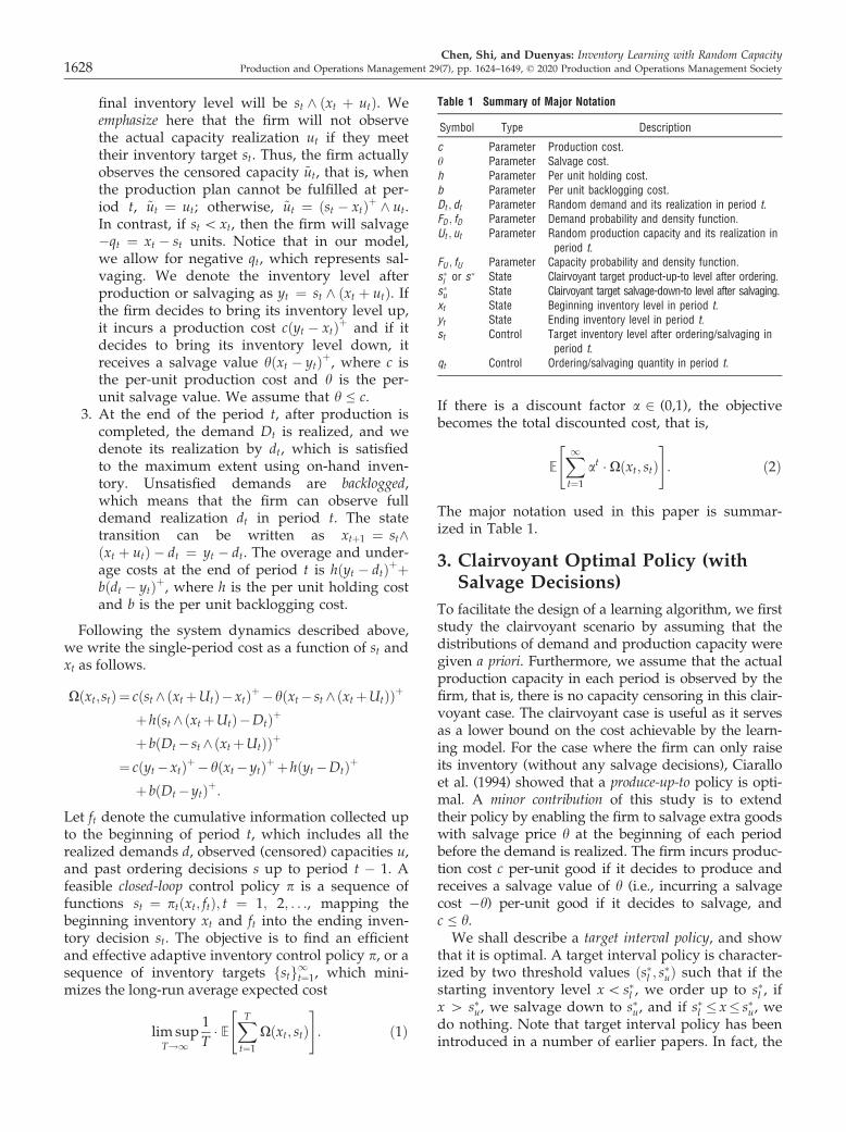
The three situations discussed above can be readilyillustrated in Figure 1. The two curves are labeled“q ≥ 0” and “q < 0,” respectively. The solid curve isthe effective cost function Ω(y), which consists ofcurve “q ≥ 0” for s ≥ x, and curve “q < 0” for s < x.

3.2. Optimal Policy for the Multi-Period Problemwith Salvaging DecisionsNext, we derive the optimal policy for the multi-per-iod problem with salvaging decisions.

PROPOSITION 2.

1. For the T-period finite-horizon problem withsalvaging decisions, a target interval policy isoptimal. More specifically, for each period t = 1,. . .,T, there exist two time-dependent threshold levels s�t;land s�t;u such that the optimal target level s�t satisfies

s�t ¼s�t;l; xt\s�t;l;xt; s�t;l � xt � s�t;u;s�t;u; xt [ s�t;u:

8><>:

2. For both the infinite horizon discounted problem (2)with salvaging decisions and the average costproblem (1) with salvaging decisions, a targetinterval policy is optimal. More specifically, thereexist two time-invariant threshold levels s�l and s�usuch that the optimal target level s�t satisfies

(a) (b) (c)

Figure 1 Illustration of a Target Interval Policy


s�t ¼s�l ; xt\s�l ;xt; s�l � xt � s�u;s�u; xt [ s�u:

8<:

Note that for the finite time horizon case, the optimaltarget level depends on a pair of time-dependent thresh-old levels, whereas for the infinite horizon case, theoptimal interval policy depends on a pair of time-invar-iant threshold levels. Since the clairvoyant benchmarkis chosen with respect to the infinite horizon problem,our goal is to find the optimal target interval ðs�l ; s�uÞ.We have shown that if the firm has the option to sal-vage extra goods at the beginning of each period, thenit will choose to salvage extra goods if the startinginventory is high enough. In the full-information pro-blem, we can immediately conclude that in the infinitehorizon problem, the salvage decision will only bemade in the first period when the initial starting inven-tory is higher than s�u. This is because after salvagingdown to s�u in the first period, the inventory level willgradually be consumed down below s�l and after that,the inventory level will never exceed s�l again, due tothe stationary demand assumption. Thus, the optimalproduce-up-to level s�l is the same as the optimal pro-duce-up-to level, denoted by s�, in Ciarallo et al. (1994)without salvaging options, and an extended myopicpolicy described therein is also optimal for the infinitehorizon average cost setting. In the remainder of thisstudy, we will use s�l and s� interchangeably. However,we must emphasize here that in the learning version ofthe problem, since we do not know the demand andcapacity distributions (and of course s�l or s

�), we needto actively explore the inventory space, and salvagingdecisions will be made in our online learning algorithm(more frequently in the beginning phase).

4. Nonparametric Learning Algorithms

As discussed in section 1, in many practical scenarios,the firm neither knows the distribution of demand Dnor the distribution of production capacity U at thebeginning of the planning horizon. Instead, the firmhas to rely on the observable demand and capacityrealizations over time to make adaptive productiondecisions. More precisely, in each period t, the firmcan observe the realized demand dt as well as theobserved production capacity ~ut. In our model, whiledt is the true demand realization (since the demandsare backlogged), the observed production capacity ~utis, in fact, censored. More explicitly, the censoredcapacity ~ut ¼ ðst � xtÞþ ^ ut. That is, suppose the firmwants to raise the starting inventory level xt to sometarget level st. If the true realized production capacityut [ ðst � xtÞþ, then the firm cannot observe theuncensored capacity realization ut. Our objective is tofind an efficient and effective learning production

control policy whose long-run average cost convergesto the clairvoyant optimal cost (had the distributionalinformation of both the random demand and the ran-dom capacity been given a priori) at a provably tightconvergence rate.

4.1. The Notion of Production CyclesIt is well-known in the literature that the optimal pol-icy for a capacitated inventory system cannot besolved myopically, that is, the control that minimizesa single-period cost is not optimal. Moreover, whencapacities are random, the per-period cost function isnon-convex, due to the fact that the decision is trun-cated by a random variable (see Chen et al. (2018) andFeng and Shanthikumar (2018)). Thus, one cannot runthe stochastic gradient descent algorithms period byperiod. To overcome this difficulty, we partition theset of time periods into carefully designed learningcycles, and update our production target levels fromcycle to cycle, instead of from period to period.We now formally define these learning cycles.

Given that we produce up to the target level st insome period t and then use the same target level st forall subsequent periods, we define a production cycle asthe set of successive periods starting from period tuntil the next period in which we are able to produceup to st again. Mathematically, let sj denote the start-ing period of the jth production cycle. Then, for anygiven initial target level s1 2 ½0;�s�, we have

s1 ¼ 1;

sj ¼ min t� sj�1 þ 1�� xt þ ut � ssj�1

n o; for all j� 2:

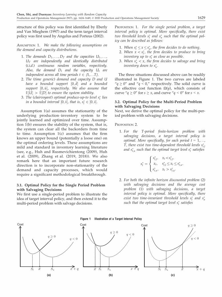
For convenience, we call ssj the cycle target level forproduction cycle j. We let lj be the cycle length of thejth production cycle, that is, lj ¼ sjþ1 � sj.Figure 2 gives a simple graphical example of a pro-

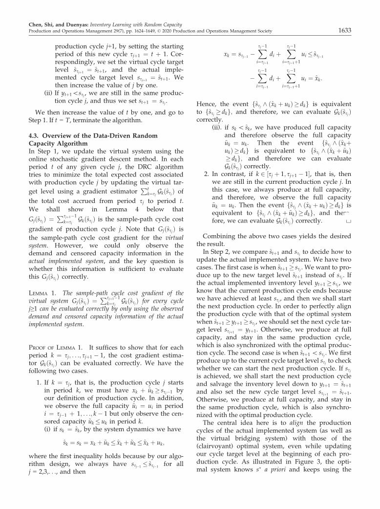
duction cycle. Suppose the target production levels5 ¼ 30 and the realized capacity levels ut ¼ 15 fort = 5,. . .,9. In periods 6,7,8, we are not able to attainthe target level s5 even if we produce the full capacityin these periods, whereas we are able to do so in per-iod 9. Therefore, this production cycle runs from per-iod 5 to period 9. Note that in period 9, we could onlyobserve the censored capacity ~u9 ¼ 11 (instead of thetrue realized capacity u9 ¼ 15), because we only needto produce 11 to attain the target level.The definition of these production cycles is moti-

vated by the idea of extended myopic policies, which weshall discuss next. In the full-information (clairvoy-ant) case with stationary demand, the structuralresults in section 3 imply that if the system starts withinitial inventory s� (for simplicity we drop the sub-script from the optimal produce-up-to level s�l Þ, thenthe optimal policy is a modified base-stock policy,that is, in each period t,


yt ¼ s�; ifxt þ ut � s�;xt þ ut; ifxt þ ut\s�:

�

In this case, our definition of production cyclesreduces to

s1 ¼ 1;

sj ¼ min t� sj�1 þ 1�� yt ¼ s�

n o; for all j� 2:

In other words, the optimal system forms asequence of production cycles whose cycle targetlevels are all set to be s�, which is also illustrated at

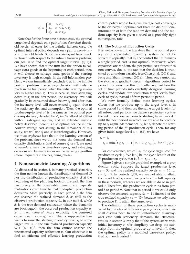
the top portion of Figure 3. Ciarallo et al. (1994)showed that the extended myopic policy, which isobtained by merely minimizing the expected totalcost within a single production cycle, is optimal.(They also provided a computationally tractable pro-cedure to compute this s� with known demand andcapacity distributions.)The above discussion has motivated us to design a

nonparametric learning algorithm that updates themodified base-stock levels in a cyclic way, in whichthe sequence of production cycle costs in our systemwill eventually converge to the production cycle costof the optimal system. We emphasize again that the(clairvoyant) optimal system does not need to salvagesince s� is known, whereas our system needs toactively explore the inventory space to learn the valueof s� and thus salvaging can happen frequently in thebeginning phase of the learning algorithm.

4.2. The Data-Driven Random Capacity AlgorithmWith the definition of production cycles, we shalldescribe our data-driven random capacity algorithm(DRC for short). The DRC algorithm keeps track oftwo systems in parallel, and also ensures that bothsystems share the same production cycles as in the

Figure 2 An Illustration of a Production Cycle

Figure 3 An Illustration of the Algorithmic Design


optimal system (which uses the same optimal base-stock level s� in every period). The optimal system isdepicted using dash-dot lines shown at the top of Fig-ure 3. The optimal system starts at optimal base-stocklevel s�, and uses s� as target level in every period.The first system that the DRC algorithm keeps track

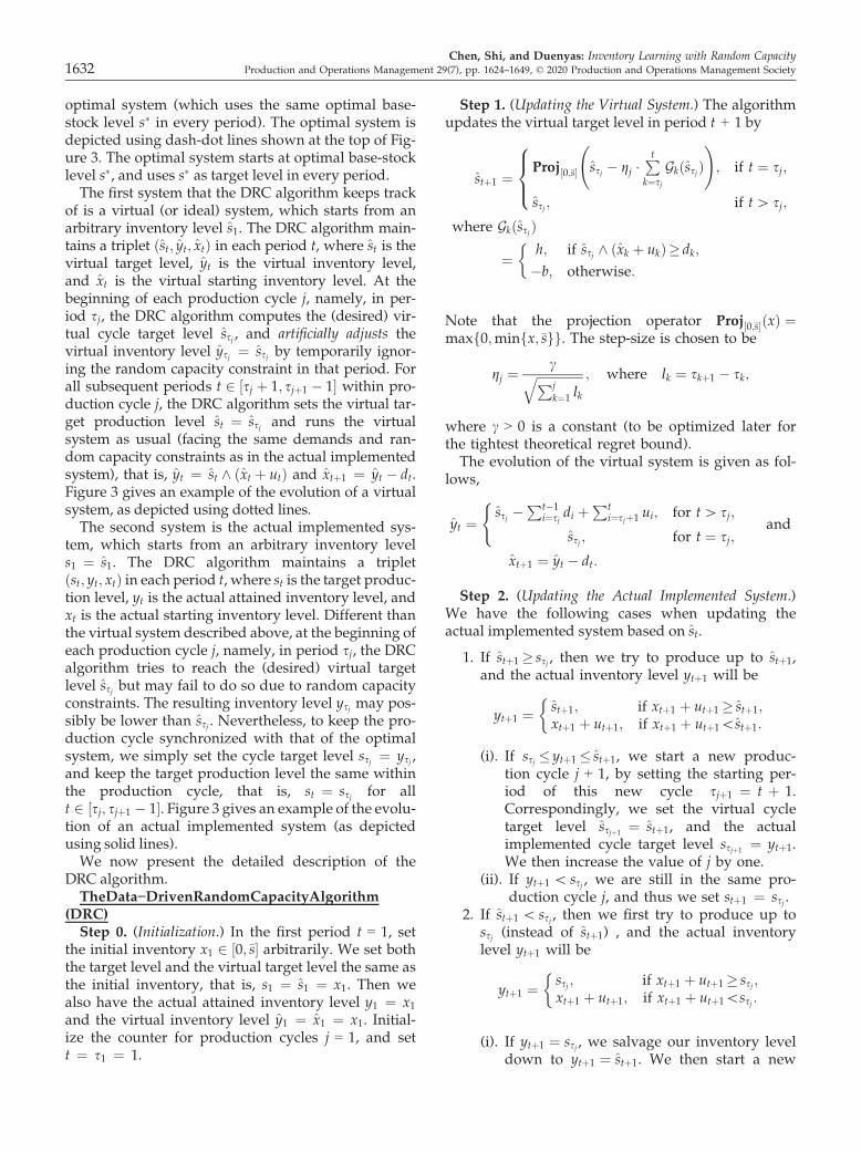
of is a virtual (or ideal) system, which starts from anarbitrary inventory level s1. The DRC algorithm main-tains a triplet ðst; yt; xtÞ in each period t, where st is thevirtual target level, yt is the virtual inventory level,and xt is the virtual starting inventory level. At thebeginning of each production cycle j, namely, in per-iod sj, the DRC algorithm computes the (desired) vir-tual cycle target level ssj , and artificially adjusts thevirtual inventory level ysj ¼ ssj by temporarily ignor-ing the random capacity constraint in that period. Forall subsequent periods t 2 ½sj þ 1; sjþ1 � 1� within pro-duction cycle j, the DRC algorithm sets the virtual tar-get production level st ¼ ssj and runs the virtualsystem as usual (facing the same demands and ran-dom capacity constraints as in the actual implementedsystem), that is, yt ¼ st ^ ðxt þ utÞ and xtþ1 ¼ yt � dt.Figure 3 gives an example of the evolution of a virtualsystem, as depicted using dotted lines.The second system is the actual implemented sys-

tem, which starts from an arbitrary inventory levels1 ¼ s1. The DRC algorithm maintains a tripletðst; yt; xtÞ in each period t, where st is the target produc-tion level, yt is the actual attained inventory level, andxt is the actual starting inventory level. Different thanthe virtual system described above, at the beginning ofeach production cycle j, namely, in period sj, the DRCalgorithm tries to reach the (desired) virtual targetlevel ssj but may fail to do so due to random capacityconstraints. The resulting inventory level ysj may pos-sibly be lower than ssj . Nevertheless, to keep the pro-duction cycle synchronized with that of the optimalsystem, we simply set the cycle target level ssj ¼ ysj ,and keep the target production level the same withinthe production cycle, that is, st ¼ ssj for allt 2 ½sj; sjþ1 � 1�. Figure 3 gives an example of the evolu-tion of an actual implemented system (as depictedusing solid lines).We now present the detailed description of the

DRC algorithm.TheData−DrivenRandomCapacityAlgorithm

(DRC)Step 0. (Initialization.) In the first period t = 1, set

the initial inventory x1 2 ½0;�s� arbitrarily. We set boththe target level and the virtual target level the same asthe initial inventory, that is, s1 ¼ s1 ¼ x1. Then wealso have the actual attained inventory level y1 ¼ x1and the virtual inventory level y1 ¼ x1 ¼ x1. Initial-ize the counter for production cycles j = 1, and sett ¼ s1 ¼ 1.

Step 1. (Updating the Virtual System.) The algorithmupdates the virtual target level in period t + 1 by

stþ1 ¼Proj½0;�s� ssj � gj �

Ptk¼sj

GkðssjÞ !

; if t ¼ sj;

ssj ; if t[ sj;

8><>:

where GkðssjÞ

¼ h; if ssj ^ ðxk þ ukÞ� dk;

�b; otherwise:

�

Note that the projection operator Proj½0;�s�ðxÞ ¼maxf0;minfx;�sgg. The step-size is chosen to be

gj ¼cffiffiffiffiffiffiffiffiffiffiffiffiffiffiffiPjk¼1 lk

q ; where lk ¼ skþ1 � sk;

where c > 0 is a constant (to be optimized later forthe tightest theoretical regret bound).The evolution of the virtual system is given as fol-

lows,

yt ¼ssj �

Pt�1i¼sj

di þPt

i¼sjþ1 ui; for t[ sj;

ssj ; for t ¼ sj;

(and

xtþ1 ¼ yt � dt:

Step 2. (Updating the Actual Implemented System.)We have the following cases when updating theactual implemented system based on st.

1. If stþ1 � ssj , then we try to produce up to stþ1,and the actual inventory level ytþ1 will be

ytþ1 ¼ stþ1; if xtþ1 þ utþ1 � stþ1;xtþ1 þ utþ1; if xtþ1 þ utþ1\stþ1:

�

(i). If ssj � ytþ1 � stþ1, we start a new produc-tion cycle j + 1, by setting the starting per-iod of this new cycle sjþ1 ¼ t þ 1.Correspondingly, we set the virtual cycletarget level ssjþ1

¼ stþ1, and the actualimplemented cycle target level ssjþ1

¼ ytþ1.We then increase the value of j by one.

(ii). If ytþ1 \ ssj , we are still in the same pro-duction cycle j, and thus we set stþ1 ¼ ssj .

2. If stþ1 \ ssj , then we first try to produce up tossj (instead of stþ1) , and the actual inventorylevel ytþ1 will be

ytþ1 ¼ ssj ; if xtþ1 þ utþ1 � ssj ;xtþ1 þ utþ1; if xtþ1 þ utþ1\ssj :

�

(i). If ytþ1 ¼ ssj , we salvage our inventory leveldown to ytþ1 ¼ stþ1. We then start a new


production cycle j+1, by setting the startingperiod of this new cycle sjþ1 ¼ t þ 1. Cor-respondingly, we set the virtual cycle targetlevel ssjþ1

¼ stþ1, and the actual imple-mented cycle target level ssjþ1

¼ stþ1. Wethen increase the value of j by one.

(ii) If ytþ1\ssj , we are still in the same produc-tion cycle j, and thus we set stþ1 ¼ ssj .

We then increase the value of t by one, and go toStep 1. If t = T, terminate the algorithm.

4.3. Overview of the Data-Driven RandomCapacity AlgorithmIn Step 1, we update the virtual system using theonline stochastic gradient descent method. In eachperiod t of any given cycle j, the DRC algorithmtries to minimize the total expected cost associatedwith production cycle j by updating the virtual tar-

get level using a gradient estimatorPt

k¼sjGkðssjÞ of

the total cost accrued from period sj to period t.

We shall show in Lemma 4 below that

GjðssjÞ ¼ Psjþ1�1

k¼sjGkðssjÞ is the sample-path cycle cost

gradient of production cycle j. Note that GjðssjÞ is

the sample-path cycle cost gradient for the virtualsystem. However, we could only observe thedemand and censored capacity information in theactual implemented system, and the key question iswhether this information is sufficient to evaluatethis GjðssjÞ correctly.

LEMMA 1. The sample-path cycle cost gradient of thevirtual system GjðssjÞ ¼ Psjþ1�1

k¼sjGkðssjÞ for every cycle

j≥1 can be evaluated correctly by only using the observeddemand and censored capacity information of the actualimplemented system.

PROOF OF LEMMA 1. It suffices to show that for eachperiod k ¼ sj; . . .; sjþ1 � 1, the cost gradient estima-tor GkðssjÞ can be evaluated correctly. We have thefollowing two cases.

1. If k ¼ sj, that is, the production cycle j startsin period k, we must have xk þ ~uk � ssj�1 byour definition of production cycle. In addition,we observe the full capacity ~ui ¼ ui in periodi ¼ sj�1 þ 1; . . .; k� 1 but only observe the cen-sored capacity ~uk � uk in period k.(i) if sk ¼ sk, by the system dynamics we have

sk ¼ sk ¼ xk þ ~uk � xk þ ~uk � xk þ uk;

where the first inequality holds because by our algo-rithm design, we always have ssj�1

� ssj�1for all

j = 2,3,. . ., and then

xk ¼ ssj�1�Xsj�1

i¼sj�1

di þXsj�1

i¼sj�1þ1

ui � ssj�1

�Xsj�1

i¼sj�1

di þXsj�1

i¼sj�1þ1

ui ¼ xk:

Hence, the event fssj ^ ðxk þ ukÞ� dkg is equivalentto fssj � dkg; and therefore, we can evaluate GkðssjÞcorrectly.

(ii). if sk \ sk, we have produced full capacityand therefore observe the full capacity~uk ¼ uk. Then the event fssj ^ ðxkþukÞ� dkg is equivalent to fssj ^ ðxk þ ~ukÞ� dkg; and therefore we can evaluateGkðssjÞ correctly.

2. In contrast, if k 2 ½sj þ 1; sjþ1 � 1�, that is, thenwe are still in the current production cycle j. Inthis case, we always produce at full capacity,and therefore, we observe the full capacity~uk ¼ uk. Then the event fssj ^ ðxk þ ukÞ� dkg isequivalent to fssj ^ ðxk þ ~ukÞ� dkg; and there-fore, we can evaluate GkðssjÞ correctly. h

Combining the above two cases yields the desiredthe result.In Step 2, we compare stþ1 and ssj to decide how to

update the actual implemented system. We have twocases. The first case is when stþ1 � ssj . We want to pro-duce up to the new target level stþ1 instead of ssj . Ifthe actual implemented inventory level ytþ1 � ssj , weknow that the current production cycle ends becausewe have achieved at least ssj , and then we shall startthe next production cycle. In order to perfectly alignthe production cycle with that of the optimal systemwhen stþ1 � ytþ1 � ssj , we should set the next cycle tar-get level ssjþ1

¼ ytþ1. Otherwise, we produce at fullcapacity, and stay in the same production cycle,which is also synchronized with the optimal produc-tion cycle. The second case is when stþ1 \ ssj . We firstproduce up to the current cycle target level ssj to checkwhether we can start the next production cycle. If ssjis achieved, we shall start the next production cycleand salvage the inventory level down to ytþ1 ¼ stþ1

and also set the new cycle target level ssjþ1¼ stþ1.

Otherwise, we produce at full capacity, and stay inthe same production cycle, which is also synchro-nized with the optimal production cycle.The central idea here is to align the production

cycles of the actual implemented system (as well asthe virtual bridging system) with those of the(clairvoyant) optimal system, even while updatingour cycle target level at the beginning of each pro-duction cycle. As illustrated in Figure 3, the opti-mal system knows s� a priori and keeps using the


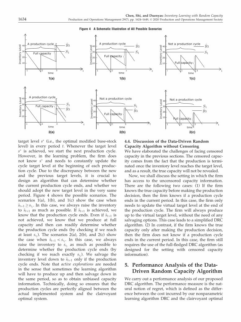
target level s� (i.e., the optimal modified base-stocklevel) in every period t. Whenever the target levels� is achieved, we start the next production cycle.However, in the learning problem, the firm doesnot know s� and needs to constantly update thecycle target level at the beginning of each produc-tion cycle. Due to the discrepancy between the newand the previous target levels, it is crucial todesign an algorithm that can determine whetherthe current production cycle ends, and whether weshould adopt the new target level in the very sameperiod. Figure 4 shows the possible scenarios. Thescenarios 1(a), 1(b), and 1(c) show the case whenstþ1 � ssj . In this case, we always raise the inventoryto stþ1 as much as possible. If stþ1 is achieved, weknow that the production cycle ends. Even if stþ1 isnot achieved, we know that we produce at fullcapacity and then can readily determine whetherthe production cycle ends (by checking if we reachat least ssj). The scenarios 2(a), 2(b), and 2(c) showthe case when stþ1 \ ssj . In this case, we alwaysraise the inventory to ssj as much as possible todetermine whether the production cycle ends (bychecking if we reach exactly ssj). We salvage theinventory level down to stþ1 only if the productioncycle ends. Note that active explorations are neededin the sense that sometimes the learning algorithmwill have to produce up and then salvage down inthe same period, so as to obtain unbiased capacityinformation. Technically, doing so ensures that theproduction cycles are perfectly aligned between theactual implemented system and the clairvoyantoptimal system.

4.4. Discussion of the Data-Driven RandomCapacity Algorithm without CensoringWe have elaborated the challenges of facing censoredcapacity in the previous sections. The censored capac-ity comes from the fact that the production is termi-nated once the inventory level reaches the target level,and as a result, the true capacity will not be revealed.Now, we shall discuss the setting in which the firm

has access to the uncensored capacity information.There are the following two cases: (1) If the firmknows the true capacity before making the productiondecision, then the firm knows if a production cycleends in the current period. In this case, the firm onlyneeds to update the virtual target level at the end ofthe production cycle. The firm will always produceup to the virtual target level, without the need of anysalvaging options. This case leads to a simplified DRCalgorithm. (2) In contrast, if the firm knows the truecapacity only after making the production decision,then the firm does not know if a production cycleends in the current period. In this case, the firm stillrequires the use of the full-fledged DRC algorithm (asdesigned for the setting with censored capacityinformation).

5. Performance Analysis of the Data-Driven Random Capacity Algorithm

We carry out a performance analysis of our proposedDRC algorithm. The performance measure is the nat-ural notion of regret, which is defined as the differ-ence between the cost incurred by our nonparametriclearning algorithm DRC and the clairvoyant optimal

1(a) 1(b) 1(c)

2(a) 2(b) 2(c)

Figure 4 A Schematic Illustration of All Possible Scenarios


cost (where the demand and production capacity dis-tribution are both known a priori). That is, for anyT ≥ 1,

RT ¼ EXTt¼1

Xðxt; stÞ � Xðxt; s�Þð Þ" #

;

where st is the target level prescribed by the DRCalgorithm for period t, and s� is the clairvoyant opti-mal target level. We note that our clairvoyant bench-mark is chosen with respect to the infinite horizonproblem, and the regret quantifies the cumulativeloss of running our learning algorithm for any T ≥ 1periods, compared to this stationary benchmark.Theorem 1 below states the main result of this study.

THEOREM 1. For stochastic inventory systems withdemand and capacity learning, the cumulative regret RT

of the data-driven random capacity algorithm (DRC) isupper bounded by Oð ffiffiffiffi

Tp Þ. In other words, the average

regret RT=T approaches to 0 at the rate of Oð1= ffiffiffiffiT

p Þ.

REMARK 1. Let l ¼ E½U� � E½D�, the differencebetween expected capacity and expected demand.We define t ¼ 2l2=ð�uþ �dÞ2 and X1 ¼ ðh _ bÞl1�Ps2

t¼s1 þ 1 Ut þPs2�1

t¼s1Dt, and then further define

a ¼ �E½X1� and r2 ¼ Var½X1� and b ¼ E½X31�. The

optimal constant c in the step size (that gives rise tothe tightest theoretical regret bound) is given by

c ¼ �sffiffiffiffiffiffiffiffiffiffiffiffiffiffiffiffiffiffiffiffiffiffiffiffiffiffiffiffiffiffiffiffiffiffiffiffiffiffiffiffiffiffiffiffiffiffiffiffiffiffiffiffiffiffiffiffiffiffiffiffiffiffiffiffiffiffiffiffiffiffiffiffiffiffiffiffiffiffiðh _ bÞ2 1

t þ 2t2 þ 2

t3� �þ 2ðh _ bÞ2 �s

lra e

6b

r3þa

r

þ2ðcþ hÞðh _ bÞ ra e6b

r3þa

r

vuut;

and the associated constant K in the regret bound ofTheorem 1 is given by

K ¼ �s

ffiffiffiffiffiffiffiffiffiffiffiffiffiffiffiffiffiffiffiffiffiffiffiffiffiffiffiffiffiffiffiffiffiffiffiffiffiffiffiffiffiffiffiffiffiffiffiffiffiffiffiffiffiffiffiffiffiffiffiffiffiffiffiffiffiffiffiffiffiffiffiffiffiffiffiffiffiffiðh _ bÞ2 1

t þ 2t2 þ 2

t3� �þ 2ðh _ bÞ2 �s

lra e

6b

r3þa

r

þ2ðcþ hÞðh _ bÞ ra e6b

r3þa

r

vuuut :

The proposed DRC algorithm is the first learningalgorithm for random capacitated inventory systems,which achieves a square-root regret rate. Moreover,this square-root regret rate is unimprovable, even forthe repeated newsvendor problem without inventorycarryover and with infinite capacity, which is a spe-cial case of our problem.

PROPOSITION 3. Even in the case of uncensored demand,the square-root regret rate is tight.

PROOF OF PROPOSITION 3. The proof follows Proposition1 in Zhang et al. (2019) for the repeated newsvendorproblem (without inventory carryover and with infi-nite capacity). h

The remainder of this study is to establish theregret upper bound in Theorem 1. For each j ≥ 1,if we adopt the cycle target level ssj and also arti-ficially set the initial inventory level xsj ¼ ssj , wecan then express the cost associated with the pro-duction cycle j as

HðssjÞ ¼Xsjþ1

t¼sjþ1

c ssj ^ xt þUtð Þ � xt� �þ

þXsjþ1�1

t¼sj

h ssj ^ xt þUtð Þ �Dt

� �þ

þ b Dt � ssj ^ xt þUtð Þ� �þ

�

¼Xsjþ1�1

t¼sjþ1

cUt þ cðssj � xsjþ1Þ

þXsjþ1�1

t¼sj


� �þ


�

¼Xsjþ1�1

t¼sjþ1

cUt þ cXsjþ1�1

t¼sj

Dt �Xsjþ1�1

t¼sjþ1

Ut

0@

1A

þXsjþ1�1

t¼sj


� �þ


�;

ð3Þ

where the second equality comes from the fact thatwe always produce at full capacity within a produc-tion cycle, except for the last period in which we areable to reach the target level. The third equalityfollows from expressing

xsjþ1¼ xsj þ

Xsjþ1�1

t¼sjþ1

Ut �Xsjþ1�1

t¼sj

Dt

¼ ssj þXsjþ1�1

t¼sjþ1

Ut �Xsjþ1�1

t¼sj

Dt:

Now, we use J to denote the total number of pro-duction cycles before period T, including possiblythe last incomplete cycle. (If the last cycle is notcompleted at T, then we truncate the cycle and alsolet sJþ1 � 1 ¼ T, that is, ssJþ1

¼ ssJ .) By the construc-tion of the DRC algorithm, we can write the cumu-lative regret as


RT ¼ EXTt¼1

Xðxt; stÞ � Xðxt; s�Þ" #

¼ EXJj¼1

HðssjÞ þXJj¼1

c ssjþ1� ssj

� �þ24

þh ssj � ssjþ1

� �þ��XJj¼1

Xsjþ1�1

t¼sj

Xðxt; s�Þ35

¼ EXJj¼1

HðssjÞ �XJj¼1

Xsjþ1�1

t¼sj

Xðxt; s�Þ24

35

þ EXJj¼1

c ssjþ1� ssj

� �þþh ssj � ssjþ1

� �þ �24

35

¼ EXJj¼1

HðssjÞ �XJj¼1

Xsjþ1�1

t¼sj

Xðxt; s�Þ24

35

þ EXJj¼1

HðssjÞ �XJj¼1

HðssjÞ24

35

þ EXJj¼1

c ssjþ1� ssj

� �þþh ssj � ssjþ1

� �þ �24

35;

where on the right-hand side of the fourth equality,the first term is the production cycle cost differencebetween using the virtual target level ssj and usingthe clairvoyant optimal target level s�. The secondterm is the production cycle cost difference betweenusing the actual implemented target level ssj andusing the virtual target level ssj . The third term isthe cumulative production and salvaging costsincurred by adjusting the production cycle targetlevels.To prove Theorem 1, it is clear that it suffices to

establish the following set of results.

PROPOSITION 4. For any J ≥ 1, there exists a constantK1 2 Rþ such that

EXJj¼1

HðssjÞ �XJj¼1

Xsjþ1�1

t¼sj

Xðxt; s�Þ24

35�K1

ffiffiffiffiT

p:


EXJj¼1

HðssjÞ �XJj¼1

HðssjÞ24

35�K2

ffiffiffiffiT

p:


EXJj¼1

c ssjþ1� ssj

� �þþ h ssj � ssjþ1

� �þ �24

35�K3

ffiffiffiffiT

p:

5.1. Several Key Building Blocks for the Proof ofTheorem 1Before proving Propositions 4– 6, we first establishsome key preliminary results.Recall that the production cycle defined in section

4.1 is the interval between successive periods inwhich the policy is able to attain a given base-stocklevel. We first show that the cumulative cost within aproduction cycle is convex in the base-stock level.

LEMMA 2. The production cycle cost Θ(s) is convex in salong every sample path.

PROOF OF LEMMA 2. It suffices to analyze the firstproduction cycle cost (with x1 ¼ s1)

Hðs1Þ ¼Xs2�1

t¼2

cUt þ cXs2�1

t¼1

Dt �Xs2�1

t¼2

Ut

!

þXs2�1

t¼1

h s1 ^ xt þUtð Þ �Dtð Þþ�þ b Dt � s1 ^ xt þUtð Þð Þþ�:

Taking the first derivative of Hðs1Þ with respect tos1, we have

H0 s1ð Þ ¼Xs2�1

t¼1

hðnþt ðs1ÞÞ � bðn�t ðs1ÞÞ� �

; ð4Þ

where nþt ðs1Þ ¼ 1 s1 �Xtt0¼1

Dt0 þXtt0¼2

Ut0 � 0

( )and

n�t ðs1Þ ¼ 1 s1 �Xtt0¼1

Dt0 þXtt0¼2

Ut0\0

( )

are indicator functions of the positive inventory left-over and the unsatisfied demand at the end of per-iod t, respectively. h

For any given d > 0, we have

H0ðs1 þ dÞ ¼Xs2�1

t¼1

h nþðs1 þ dÞ� �� b n�ðs1 þ dÞð Þ� :

It is clear that when the target level increases, thepositive inventory left-over will also increase, i.e,

nþðs1 þ dÞ� nþðs1Þ: Similarly, we also have n�ðs1 þ dÞ� n�ðs1Þ: Therefore, we have H0ðs1 þ dÞ � H0ðs1Þ forany value of s1, and thus Θ(�) is convex.


Given the convexity result, our DRC algorithmupdates base-stock levels in each production cycle.Note that these production cycles (as renewal pro-cesses) are not a priori fixed but are sequentially trig-gered as demand and capacity realize over time.Therefore, we need to develop an upper bound on themoments of a random production cycle. The proof ofLemma 3 relies on building an upward drifting ran-dom walk with Ut as upward step and Dt as down-ward step, wherein the chance of hitting a level belowzero is exponentially small due to concentrationinequalities. Since the ending of a production cyclecorresponds to the situation where the random walkhits zero, the second moment of its length of the cur-rent production cycle can be bounded.

LEMMA 3. The second moment of the length of a produc-tion cycle E½l2j � is bounded for all cycle j.

PROOF OF LEMMA 3. By the definition of a produc-tion cycle in section 4.1, we have

Pflj ¼ lg

¼ P Usjþ1 �Dsj\0; . . .;Xsjþl�1

t¼sjþ1

Ut �Xsjþl�2

t¼sj

Dt\0;

8<:Xsjþl

t¼sjþ1

Ut �Xsjþl�1

t¼sj

Dt � 0

9=;:

Since Dt and Ut are both i.i.d., so is lj. Let Mk be anupward drifting random walk, more precisely,

Mk ¼Pkt¼1

ðUt �DtÞ: Then we have, by letting l ¼

E½Ut �Dt� and t ¼ 2l2=ð�u þ �dÞ2,

E l2j

h i¼X1k¼1

k2P M1\0; ;Mk�1\0;Mk � 0ð Þ

�X1k¼1

k2P Mk�1 � ðk� 1Þl\� ðk� 1Þlð Þ

�X1k¼1

k2 exp � 2ðk� 1Þl2�uþ �d� �2

!

�Z 1

0

ðkþ 1Þ2 exp � 2kl2

�uþ �d� �2

!

dk ¼ 1

tþ 2

t2þ 2

t3\1;

where the second inequality follows from theHoeffding’s inequality.

We also need to develop an upper bound on thecycle cost gradient.

LEMMA 4. For any j ≥ 1, the function GjðsÞ ¼Psjþ1�1t¼sj GtðsÞ is the sample-path cycle cost gradient of

production cycle j, where s is the cycle target level.Moreover, Gjð�Þ has a bounded second moment, that is,E½G2

j ðsÞ�\1 for any s.

PROOF OF LEMMA 4. From the definition of GjðsÞ and(4), it is clear that

GjðsÞ ¼Xsjþ1�1

t¼sj

GtðsÞ ¼Xsjþ1�1

t¼sj

hðnþt ðsÞÞ � bðn�t ðsÞÞ� ¼ H0ðsÞ:

Moreover, we have

E G2j ðsÞ

h i¼ E

Xs2�1

t¼1

hðnþt ðs1ÞÞ � bðn�t ðs1ÞÞ� � !2

24

35

� E h _ bð Þ2l2jh i

¼ h _ bð Þ2E l2j

h i\1;

where the last inequality follows from Lemma 3. h

5.2. Proof of Proposition 4Proposition 4 provides an upper bound on the pro-duction cycle cost difference between using the vir-tual target level ssj and using the clairvoyant optimaltarget level s�. The proof follows a similar argumentused in the general stochastic approximation litera-ture (see Nemirovski et al. (2009)) as well as theonline convex optimization literature (see Hazan(2016)). The main point of departure is due to the apriori random cycles, and therefore the proof reliescrucially on Lemmas 3 and 4 previously established.By optimality of s�, we have E½Xðs�; s�Þ� ¼

infxfE½Xðx; s�Þ�g, that is, s� minimizes the expected sin-gle period cost. Also notice that the length of a pro-duction cycle is independent of the cycle target levelbeing implemented. Thus, we have

EXJj¼1

HðssjÞ �XJj¼1

Xsjþ1�1

t¼sj

Xðxt; s�Þ24

35

� EXJj¼1

HðssjÞ �XJj¼1

Xsjþ1�1

t¼sj

Xðs�; s�Þ24

35

¼ EXJj¼1

HðssjÞ �Hðs�Þ� �2

435:

ð5Þ

By the sample path convexity of Θ(�) shown inLemma 2, we have

EXJj¼1

HðssjÞ �Hðs�Þ� �2

435�

XJj¼1

E rHðssjÞðssj � s�Þh i

¼XJj¼1

E GjðssjÞðssj � s�Þh i

: ð6Þ


By the definition of ssjþ1in the DRC algorithm,

E ssjþ1� s�

� �2� E ssj � gjGjðssjÞ � s�� 2

¼E ssj � s�� 2

þE gjGjðssjÞ� �2

� E 2gjGjðssjÞðssj � s�Þh i

¼E ssj � s�� 2

þE½gj�E GjðssjÞ� �2

� 2E½gj�E GjðssjÞðssj � s�Þh i

;

where the second equality holds because the step-size gj is independent of ssj and GjðssjÞ. Thus,

E GjðssjÞðssj � s�Þh i

� 1

2E½gj�E ssj � s�� 2

�E ssjþ1� s�

� �2 �

þ1

2E gj GjðssjÞ

� �2 �: ð6Þ

Combining (6) and (7), we have

XJj¼1

E rHðssjÞðssj � s�Þh i

�XJj¼1

1

2E½gj�E ssj � s�� 2

�E ssjþ1� s�

� �2 �

þ 1

2E gj GjðssjÞ

� �2 ��

¼ 1

2E½g1�E ss1 � s�ð Þ2� 1

2E½gj�E ssjþ1

� s�� 2

þ 1

2

XJj¼2

1

E½gj�� 1

E½gj�1�

!E ssj � s�� 2

þXJj¼1

E gj GjðssjÞ� �2 �

2

� 2�s21

2E½g1�þ 1

2

XJj¼2

1

E½gj�� 1

E½gj�1�

!0@

1A

þE½ GjðssjÞ� �2

�2

XJj¼1

E½gj�

¼ �s2

E½gJ�þE½ GjðssjÞ� �2

�2

XJj¼1

E½gj�K1

ffiffiffiffiT

p;

where the last inequality holds due to Lemma 4(the bounded second moment of G(�)) and

XJj¼1

E½gj� ¼ cXJj¼1

E 1=

ffiffiffiffiffiffiffiffiffiffiffiXji¼1

li

vuut24

35� c

XTt¼1

1=ffiffit

p� 2c

ffiffiffiffiT

p:

5.3. Proof of Proposition 5Proposition 5 provides an upper bound on the pro-duction cycle cost difference between using theactual implemented target level ssj and using thevirtual target level ssj . The main idea of this proofon a high level is to set up an upper boundingstochastic process that resembles the waiting timeprocess of a GI/GI/1 queue. A similar argumentappeared Huh and Rusmevichientong (2009) andShi et al. (2016). There are two differences. First,the mapping to the waiting time process is moreinvolved in the presence of random capacities. Inthe above two papers, the resulting level is alwayshigher than the target level, whereas the resultinglevel could be either higher or lower than the tar-get level in our setting. Second, this study needs tobound the difference in cycle target levels (relyingon Lemmas 3 and 4), rather than per-period targetlevels.By the definition of production cycle cost (3), we

have

E HðssjÞ �HðssjÞh i

¼EXsjþ1�1

t¼sj


� �þ24

þb Dt � ssj ^ xt þUtð Þ� �þ

�

�Xsjþ1�1

t¼sj


� �þ

þb Dt � ssj ^ xt þUtð Þ� �þ��

� EXlj�1

t¼1

ðh _ bÞjssj � ssj j" #

� E½lj�ðh _ bÞjssj � ssj j;

where the second inequality holds due to theWald’s Theorem using the fact that lj is indepen-dent of ssj and ssj , and the first inequality followsfrom the fact that for any t 2 ½sj; sjþ1 � 1�, wehave

E h ssj ^ xt þUtð Þ �Dt

� �þþb Dt � ssj ^ xt þUtð Þ� �þ �

� h ssj ^ xt þUtð Þ �Dt

� �þþb Dt � ssj ^ xt þUtð Þ� �þ ��

� E h ssj ^ xt þUtð Þ � ssj ^ xt þUtð Þ� �þ

þb ssj ^ xt þUtð Þ � ssj ^ xt þUtð Þ� �þ�

�ðh _ bÞ ssj � ssj

�� :


Thus, to prove Proposition 5, it suffices to prove

EXJj¼1

HðssjÞ �XJj¼1

HðssjÞ24

35� E½lj�ðh

_ bÞEXJj¼1

jssj � ssj j24

35�Oð

ffiffiffiffiT

pÞ:

Next, we consider an auxiliary stochastic processðZj j j� 0Þ defined by

Zjþ1 ¼ Zj þc�jffiffiffiffiffiffiffiffiffiPjt¼1

lt

s � mj

266664

377775

þ

; ð8Þ

where the random variables �j ¼ ðh _ bÞlj, and

mj ¼Psjþ1

t¼sjþ1 Ut �Psjþ1�1

t¼sj Dt, and Z0 ¼ 0. Moreover,

since we know that in period sjþ1, the production

cycle ends, we must have

mj ¼Xsjþ1

t¼sjþ1

Ut �Xsjþ1�1

t¼sj

Dt � 0:

Now we want to relate jssj � ssj j to the stochasticprocess defined above. We can see from the DRCalgorithm that the only situation when the virtualtarget level cannot be achieved is when ssj [ ssj .When ssj � ssj , we can salvage extra inventory andachieve the virtual target level. Therefore, we relatejssj � ssj j with the stochastic process Zj.

LEMMA 5. For any j≥1,

EXJj¼1

jssj � ssj j24

35� E

XJj¼1

Zj

24

35;

where fZj; j� 1g is the stochastic process we defineabove.

PROOF OF LEMMA 5. All the stochastic comparisonswithin this proof are with probability one. Whenssjþ1

\ xsjþ1þUsjþ1

, we have ssjþ1� ssjþ1

¼ 0�Zjþ1.

When ssjþ1[ xsjþ1

þUsjþ1, we have ssjþ1

¼ xsjþ1

þUsjþ1¼ ssj �

Psjþ1�1t¼sj Dt þ

Psjþ1�1t¼sjþ1 Ut þUsjþ1. There-

fore, we have

ssjþ1� ssjþ1

�� ¼ ssjþ1� ssjþ1

¼ Proj½0;�s� ssj � gjGjðssjÞ� �

� ssjþ1� Proj½0;�s� ssj � gjGjðssjÞ

� �� ssjþ1

ssj � gjGjðssjÞ�� ssj þ

Xsjþ1�1

t¼sj

Dt �Xsjþ1�1

t¼sjþ1

Ut

0@

1A�Usjþ1

� ssj � ssj � gjGjðssjÞ�� þ Xsjþ1�1

t¼sj

Dt �Xsjþ1�1

t¼sjþ1

Ut

0@

1A�Usjþ1

� ssj � ssj

�� þ gjGjðssjÞ�� Xsjþ1�1

t¼sjþ1

Ut �Xsjþ1�1

t¼sj

Dt

0@

1A

� ssj � ssj

�� þ gjðh _ bÞ � lj �Xsjþ1�1

t¼sjþ1

Ut �Xsjþ1�1

t¼sj

Dt

0@

1A;

where the first equality holds because following theDRC algorithm, we always have ssj � ssj . The thirdinequality holds because ssj is always nonnegative.This is because the virtual target level is truncatedto be nonnegative all the time, and we update theactual implemented target level when the produc-tion cycle ends, which means after the previousactual implemented target level is achieved. Sinces1 � 0, ssj � 0 for all j. The fourth inequality holdsbecause of the triangular inequality and the lastinequality holds because jGjðssjÞj � ðh _ bÞ � lj. h

Therefore, from the above claim, we have

ssjþ1� ssjþ1

�� jssj � ssj j þ gjðh _ bÞljh

�Xsjþ1�1

t¼sjþ1

Ut �Xsjþ1�1

t¼sj

Dt

0@

1A35þ

:

Comparing to (8), we have

gjðh _ bÞlj �c�jffiffiffiffiffiffiffiffiffiPjt¼1

lt

s ;

and since s1 � s1 ¼ 0, it follows, from the recursivedefinition of Zj, that jssjþ1

� ssjþ1j �Zjþ1 holds with

probability one. Summing up both sides of theinequality completes the proof.We observe that the stochastic process Zj is very

similar to the waiting time in a GI/GI/1 queue, except

that the service time is scaled by c=ffiffiffiffiffiffiffiffiffiffiffiffiffiffiPj

i¼1 li

qin each

production cycle j. Now consider a GI/GI/1 queueðWjjj� 0Þ defined by the following Lindley’s equa-

tion:W0 ¼ 0, and

Wjþ1 ¼ Wj þ �j � mj� þ

; ð9Þ

where the sequences �j and mj consist of indepen-dent and identically distributed random variables


(only dependent upon the distributions of D and U).Let u0 ¼ 0, u1 ¼ infft� 1 : Wj ¼ 0g and for t ≥ 1,utþ1 ¼ infft [ ut : Wj ¼ 0g. Let Bt ¼ ut � ut�1.The random variable Wj is the waiting time of thejth customer in the GI/GI/1 queue, where the inter-arrival time between the jth and jþ 1th customers isdistributed as mj, and the service time is distributedas �j. Then, Bt is the length of the tth busy period.Let q ¼ E½�1�=E½m1� represent the system utilization.Note that if q < 1, then the queue is stable, and therandom variable Bt is independent and identicallydistributed.We invoke the following result from Loulou (1978)

to bound E½Bt�, the expected busy period of a GI/GI/1queue with inter-arrival distribution m and servicetime k.

LEMMA 6. (Loulou (1978)) Let Xj ¼ �j � mj, anda ¼ �E½X1�. Let r2 be the variance of X1. If E½X1�3 ¼b\1, and q < 1,

E½B1� � raexp

6b3

r3þ ar

�:

For each n ≥ 1, let the random variable i(n) denotethe index t such that Bt contains n. This means thatthe nth customer is within the BiðnÞ busy period. SinceBt is i.i.d., we know that E½BiðnÞ� ¼ E½Bt� ¼ E½B1�:

LEMMA 7. For any period t≥1, we have

EXJj¼1

Zj

24

35� 2cðh _ bÞE½B1�

ffiffiffiffiT

p:

PROOF OF LEMMA 7. As defined above, the stochastic

process Zjþ1 ¼"Zj þ c�jffiffiffiffiffiffiffiffiffiffiffiffiPj

i¼1li

q � mj

#þ. Since Zj can be

interpreted as the waiting time in the GI/GI/1queueing system, we can rewrite Zj as

Zj ¼Xjj0¼1

c�j0ffiffiffiffiffiffiffiffiffiffiffiffiffiffiPj0i¼1 li

q � mj0

0B@

1CA1 j0 2 BiðjÞ�

�Xjj0¼1


q 1 j0 2 BiðjÞ�

:

ð10Þ

We then bound the total waiting time of sequenceZj by only considering the cumulative service timesas follows:

EXJj¼1

Zj

24

35 ¼E

XJj¼1

Xjj0¼1


q 1½j0 2 BiðjÞ�

264

375

� EXJj¼1

XJj0¼1

cðh _ bÞlj0ffiffiffiffiffiffiffiffiffiffiffiffiffiffiPj0i¼1 li

q 1½j0 2 BiðjÞ�

264

375

� EXJj0¼1


q XJj¼1

1½j0 2 BiðjÞ�

264

375

¼ EXJj0¼1


q Biðj0Þ

264

375

� EXTt¼1

cðh _ bÞffiffit

p BiðtÞ

" #;

where the last inequality holds because

XJj0¼1

lj0ffiffiffiffiffiffiffiffiffiffiffiffiffiffiPj0i¼1 li

q �XTt¼1

1ffiffit

p ; where T ¼XJj0¼1

lj0 :

Thus, we have

EXJj¼1

Zj

24

35� E

XTt¼1

cðh _ bÞffiffit

p BiðtÞ

" #

¼ cðh _ bÞEXTt¼1

1ffiffit

p" #

E½BiðtÞ� � 2cðh _ bÞffiffiffiffiT

pE½B1�;

ð11Þ

where the last inequality follows from the fact thatPTt¼1

1ffiffit

p � 2ffiffiffiffiT

p � 1: Combining 10 and 11 completesthe proof. h

Combining Lemmas 5 and 7, we have

EXJj¼1

HðssjÞ �XJj¼1

HðssjÞ24

35� E

XJj¼1

cðh _ bÞðssj � ssjÞ24

35

� cðh _ bÞE½l1�EXJj¼1

Zj

24

35

� 2cðh _ bÞ2E½l1�E½B�ffiffiffiffiT

p;

where both E½B� and E½l1� are bounded constants.This completes the proof for Proposition 5.

5.4. Proof of Proposition 6Proposition 6 provides an upper bound on the cumu-lative production and salvaging costs incurred byadjusting the production cycle target levels.The main idea of this proof on a high level is to use

the fact that the cycle target levels of the actual


implemented system are getting closer to the ones ofthe virtual system over time, and each change in thecycle target level can be sufficiently bounded, result-ing in an upper bound on the cumulative productionand salvaging costs.

EXJj¼1

c ssjþ1� ssj

� �þ24

35� E

XJj¼1

c ssjþ1� ssj

� �þ24

35

¼EXJj¼1

c Proj½0;�s� ssj � gj � GjðssjÞ� �

� ssj

� �þ24

35

� EXJj¼1

c ssj � gj � GjðssjÞ� �

� ssj

� �þ24

35

� EXJj¼1

c ssj � ssj

�� þXJj¼1

c gj � GjðssjÞ��

24

35�K4

ffiffiffiffiT

p;

where K4 is some positive constant. The result trivi-ally holds if ssjþ1

� ssj . Now, consider the case where

ssjþ1[ ssj , that is, the firm produces. The first ine-

quality holds because if the firm produces, we musthave ssjþ1

� ssjþ1by the construction of DRC. The sec-

ond inequality holds because ssj � 0. The third

inequality holds by the triangular inequality. The

last inequality is due to the fact thatPJ

j¼1 ssj � ssj

�� Oð ffiffiffiffi

Tp Þ from Proposition 5, and

XJj¼1

c gj � GjðssjÞ�� ccðh _ bÞ

XJj¼1

ljffiffiffiffiffiffiffiffiffiPji¼1

li

s � 2ccðh _ bÞffiffiffiffiT

p:

Similarly,

EXJj¼1

hðssj � ssjþ1Þþ

24

35 ¼ E

XJj¼1

hðssj � ssjþ1Þþ

24

35

¼EXJj¼1

h ssj � Proj½0;�s� ssj � gj � GjðssjÞ� �� þ2

435

� EXJj¼1

h ssj � ssj � gj � GjðssjÞ� �� þ2

435

� EXJj¼1

h ssj � ssj

�� þXJj¼1

h gj � GjðssjÞ��

24

35�K5

ffiffiffiffiT

p;

where K5 is some positive constant. The result trivi-ally holds if ssj � ssjþ1

. Now, consider the case wheressj [ ssjþ1

, that is, the firm salvages. The first equal-ity holds because if the firm salvages, we must havessjþ1

¼ ssjþ1by the construction of DRC. The first

inequality holds because �s � ssj . The second inequal-ity holds by the triangular inequality. The lastinequality follows the same idea as in the first partof this section.Combing the above two parts completes the proof

of Proposition 6.Finally, Theorem 1 is a direct consequence of

Propositions 4–6, which gives us the desired regretupper bound.

6. Numerical Experiments

We conduct numerical experiments to demonstratethe efficacy of our proposed DRC algorithm. To thebest of our knowledge, we are not aware of any exist-ing learning algorithms that are applicable to randomcapacitated inventory systems. Thus, we havedesigned two simple heuristic learning algorithms(that are intuitively sound and practical), and usethem as benchmarks to validate the performance ofthe DRC algorithm. Our results show that the perfor-mance of the DRC algorithms is superior to these twobenchmarking heuristics both in terms of consistencyand convergence rate. All the simulations were imple-mented on an Intel Xeon 3.50GHz PC.

6.1. Design of ExperimentsWe conduct our numerical experiments using a nor-mal distribution for the random demand and a mix-ture of two normal distributions for the randomcapacity. More specifically, we set the demand to beNð10; 32Þ. We test four different capacity distribu-tions, namely, a mixture of 20% Nð5; 12Þ and 80%Nð14; 42Þ, a mixture of 20% Nð5; 12Þ and 80% Nð17;52Þ, a mixture of 20% Nð5; 12Þ and 80% Nð20; 62Þ, andalso a mixture of 20% Nð5; 32Þ and 80% Nð17; 52Þ. Thedistributions correspond to environments where theproduct capacity is subject to downtime. Clearly, in aproduction environment, capacity may be random evenif no significant downtime occurs (e.g., due to varia-tions in operator speed). However, machine downtimecan significantly impact capacity. These examples cor-respond to situations where the production systemexperiences downtime that affects capacity with 20%probability. (We have experimented with other exam-ples of downtime and obtained similar results.)The production cost c = 10, and the salvaging value

is set to be half of the production cost, that is, h = 5.The backlogging cost is linear in backorder quantity,with per-unit cost b = 10, and the holding cost is 2%per period of the production cost, that is, h = 0.2. Weset the time horizon T = 1000, and compare the aver-age cost of our DRC algorithm with that of the twobenchmarking heuristic algorithms (described below)as well as the clairvoyant optimal cost over 1000periods.


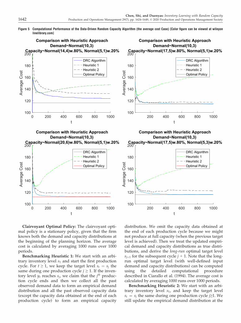
Clairvoyant Optimal Policy: The clairvoyant opti-mal policy is a stationary policy, given that the firmknows both the demand and capacity distributions atthe beginning of the planning horizon. The averagecost is calculated by averaging 1000 runs over 1000periods.Benchmarking Heuristic 1: We start with an arbi-

trary inventory level s1 and start the first productioncycle. For t ≥ 1, we keep the target level st ¼ sj thesame during one production cycle j ≥ 1. If the inven-tory level yt reaches sj, we claim that the jth produc-tion cycle ends and then we collect all the pastobserved demand data to form an empirical demanddistribution and all the past observed capacity data(except the capacity data obtained at the end of eachproduction cycle) to form an empirical capacity

distribution. We omit the capacity data obtained atthe end of each production cycle because we mightnot produce at full capacity (when the previous targetlevel is achieved). Then we treat the updated empiri-cal demand and capacity distributions as true distri-butions, and derive the long-run optimal target levelsjþ1 for the subsequent cycle j + 1. Note that the long-run optimal target level (with well-defined inputdemand and capacity distributions) can be computedusing the detailed computational proceduredescribed in Ciarallo et al. (1994). The average cost iscalculated by averaging 1000 runs over 1000 periods.Benchmarking Heuristic 2: We start with an arbi-

trary inventory level s1, and keep the target levelst ¼ sj the same during one production cycle j≥1. Westill update the empirical demand distribution at the

0 200 400 600 800 1000t

100

120

140

160

180

200

Ave

rage

Cos

t

Comparison with Heuristic ApproachDemand~Normal(10,3)

Capacity~Normal(14,4)w.80%, Normal(5,1)w.20%

DRC AlgorithmHeuristic 1Heuristic 2Optimal Policy

200 400 600 800 1000t

100

120

140

160

180

200

Ave

rage

Cos

t




0 200 400 600 800 1000t

100

120

140

160

180

200

Ave

rage

Cos

t




200 400 600 800 1000t

100

120

140

160

180

200

Ave

rage

Cos

t




Figure 5 Computational Performance of the Data-Driven Random Capacity Algorithm (the average cost Case) [Color figure can be viewed at wileyonlinelibrary.com]


www.wileyonlinelibrary.com


end of each production cycle using all past observeddemand data. However, in the first N = 10 periods,we always try to produce up to the maximum capac-ity �u, and we form the empirical capacity distributionusing only these N full capacity sample points, andtreat the empirical capacity distribution as the truecapacity distribution for the rest of decision horizon.At the end of each production cycle, we still collect allthe past observed demand data to form an empiricaldemand distribution, and similar to heuristic 1, derivethe long-run optimal target level for the subsequentcycle together with the empirical capacity distribu-tion. In other words, in the first N periods, we alwaysproduce up to the full capacity instead of the targetlevel to get true information of the capacity, and afterN periods, we carry out a regular modified base-stockpolicy. The average cost is calculated by averaging1000 runs over 1000 periods. We have experimentedwith N values different than 10 and our results aresimilar to those we report below.

6.2. Numerical Results and FindingsThe numerical results are presented in Figure 5. Weobserve that Heuristic 1 is inconsistent, that is, it failsto converge to the clairvoyant optimal cost. This isbecause even if we collect all the capacity data onlywhen we produce at full capacity, the empirical distri-bution formed by these data is still biased (as thecapacity data we observe is smaller than the truecapacity). Heuristic 2 performs better than Heuristic1, but still suffers from inconsistency.Comparing to the benchmarking heuristic algo-

rithms, the DRC algorithm converges to the clairvoy-ant optimal cost consistently and also at a much fasterrate. We can also observe that when the capacity uti-lization (defined as the mean demand over the meancapacity) increases, the convergence rate slows down.This is because when the capacity utilization is high,it generally takes more periods for the system to reachthe previous target level, resulting in longer produc-tion cycle length and slower updating frequency.Finally, we find that increasing the variability of dis-tributions does not affect the performance of the DRCalgorithm.

6.3. Extension to the Discounted Cost CaseWe also conduct numerical experiments for the dis-counted cost case. More specifically, we choose thedemand to be Nð10; 32Þ and the production capacityto be a mixture of 20%Nð5; 12Þ and 80%Nð14; 42Þ. Thetotal cost can be written as

PTt¼1 a

tXðxt; stÞ where0 < a < 1 is the discount factor and Xðxt; stÞ is the sin-gle period cost. We compare our DRC algorithm withthe optimal policy and two benchmarking heuristicsunder a = 0.995,0.99,0.97,0.95. The production, sal-vaging, backlogging, and holding costs are kept the

same as the previous numerical experiment, that is,c = 10, h = 5, b = 10, h = 0.2. We compare the totalcost up to T = 1000 periods. To adapt our DRC algo-rithm to the discounted cost case, we slightly modifyour updating strategy in Step 1 as follows:

GkðssjÞ ¼at�sj h; if ssj ^ ðxk þ ukÞ� dk;

�at�sj b; otherwise:

�

where t� sj is the time elapsed counting from thebeginning of the current production cycle. Thenumerical results are presented in Figure 6. Weobserve that the DRC algorithm clearly outperformsthe two benchmarking heuristics in terms of thetotal discounted cost.

7. Concluding Remark

In this study, we have proposed a stochastic gradientdescent type of algorithm for the stochastic inventorysystems with random production capacity con-straints, where the capacity is censored. Our algo-rithm utilizes the fact that the clairvoyant optimalpolicy is the extended myopic policy and updates thetarget inventory level in a cyclic manner. We haveshown that the average T-period cost of our algorithmconverges to the optimal cost at the rate of Oð1= ffiffiffiffi

Tp Þ,

which is the best achievable convergence rate. To thebest of our knowledge, our study is the first paper tostudy learning algorithms for stochastic inventorysystems under uncertain capacity constraints. Wehave also compared our algorithm with two strawheuristic algorithms that are easy to use, and we haveshown that our proposed algorithm performs signifi-cantly better than the heuristics in both consistencyand efficiency. Indeed, our numerical experimentshave shown that with censored capacity information,the heuristics may not converge to the optimal policy.We leave an important open question on how to

design an efficient and effective learning algorithmfor the capacitated inventory systems with lost-salesand censored demand. In this study, with backloggeddemand, the length of the production cycle is inde-pendent of the target level, and therefore, the produc-tion cycles in our proposed algorithm and the optimalsystem are perfectly aligned. With lost-sales and cen-sored demand, the length of the production cyclebecomes dependent on the target level, and compar-ing any two feasible policies becomes much morechallenging, which would require significantly newideas and techniques.Finally, we would also like to remark the connec-

tion between our online learning algorithm and deepreinforcement learning (DRL) algorithms. Needless tosay, DRL is very popular nowadays and can be usedto solve stochastic problems involving learning. We


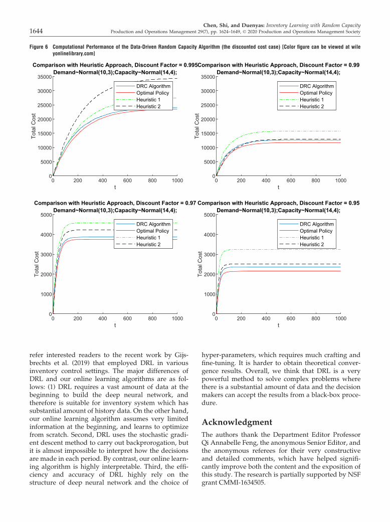
refer interested readers to the recent work by Gijs-brechts et al. (2019) that employed DRL in variousinventory control settings. The major differences ofDRL and our online learning algorithms are as fol-lows: (1) DRL requires a vast amount of data at thebeginning to build the deep neural network, andtherefore is suitable for inventory system which hassubstantial amount of history data. On the other hand,our online learning algorithm assumes very limitedinformation at the beginning, and learns to optimizefrom scratch. Second, DRL uses the stochastic gradi-ent descent method to carry out backprorogation, butit is almost impossible to interpret how the decisionsare made in each period. By contrast, our online learn-ing algorithm is highly interpretable. Third, the effi-ciency and accuracy of DRL highly rely on thestructure of deep neural network and the choice of

hyper-parameters, which requires much crafting andfine-tuning. It is harder to obtain theoretical conver-gence results. Overall, we think that DRL is a verypowerful method to solve complex problems wherethere is a substantial amount of data and the decisionmakers can accept the results from a black-box proce-dure.

Acknowledgment

The authors thank the Department Editor ProfessorQi Annabelle Feng, the anonymous Senior Editor, andthe anonymous referees for their very constructiveand detailed comments, which have helped signifi-cantly improve both the content and the exposition ofthis study. The research is partially supported by NSFgrant CMMI-1634505.

0 200 400 600 800 1000t

0

5000

10000

15000

20000

25000

30000

35000

Tota

l Cos

t

Comparison with Heuristic Approach, Discount Factor = 0.99Demand~Normal(10,3);Capacity~Normal(14,4);

DRC AlgorithmOptimal PolicyHeuristic 1Heuristic 2

0 200 400 600 800 1000t

0

1000

2000

3000

4000

5000

Tota

l Cos

t



0 200 400 600 800 1000t

0

1000

2000

3000

4000

5000

Tota

l Cos

tComparison with Heuristic Approach, Discount Factor = 0.95

Demand~Normal(10,3);Capacity~Normal(14,4);


0 200 400 600 800 1000t

0

5000

10000

15000

20000

25000

30000

35000

Tota

l Cos

t



Figure 6 Computational Performance of the Data-Driven Random Capacity Algorithm (the discounted cost case) [Color figure can be viewed at wileyonlinelibrary.com]




Appendix: Technical Proofs for Section 3

PROOF OF PROPOSITION 1. To prove the target intervalpolicy, we write the optimal single-period cost func-tion as follows.

E Xðx; sÞ½ � ¼ min mins� x

E Xþðx; sÞ½ �;mins\x

E X�ðx; sÞ½ ��

;

ðA1Þ

where

E Xþðx; sÞ½ � ¼ c � ð1� FUðs� xÞÞðs� xÞ

þ c �Z s�x

0

rfUðrÞdrþ ð1� FUðs� xÞÞZ 1

sbðz� sÞfDðzÞdzþ

Z s

0

hðs� zÞfDðzÞdz �

þZ s�x

0

Z 1

xþrbðz� x� rÞfDðzÞdzfUðrÞdr

þZ s�x

0

Z xþr

0

hðxþ r� zÞfDðzÞdzfUðrÞdr;ðA2Þ

E X�ðx; sÞ½ � ¼ h � ðs� xÞ þZ 1

sbðz� sÞfDðzÞdz

þZ s

0

hðs� zÞ fDðzÞ dz�: ðA3Þ

Notice that we produce up to s when s ≥ x, andsalvage down to s when s < x.We shall explain that in (A2) we condition on the

event s ≤ (x+U), which has a probability of ð1�FUðs� xÞÞ, we have s ^ ðxþUÞ ¼ s and apply thestandard newsvendor integral E½s�D�þ þ E½D� s�þ¼ R s

0 ðs� zÞdzþ R1s ðz� sÞdz. Similarly conditioningon the event s > (x+U), which has a probability ofFUðs� xÞ ¼ R s�x

0 fUðrÞdr, we have s ^ ðxþUÞ ¼xþU and also apply the standard newsvendor inte-gral. Allowing for salvaging, the target level s canalways be achieved in (A3).To show a target interval policy is optimal, we first

show that (A2) and (A3) have global minimizers s�land s�u, respectively. Then, we show that 0� s�l� s�u \1. Finally, we discuss different strategiesbased on different starting inventory levels to implythat a target interval policy is optimal.By applying the Leibniz integral rule, the first par-

tial derivative of (A2) with respect to s is

@

@sE Xþðx; sÞ½ � ¼ ð1� FUðs� xÞÞ

cþZ 1

s

@

@sbðz� sÞ fDðzÞ dzþ

Z s

0

@

@shðs� zÞfDðzÞdz

�:

It can be easily solved that the solution to the first-order optimality, denoted by s�l , is

s�l ¼ F�1D

b� c

hþ b

�

and

cþZ 1

s�l

@

@sbðz� sÞfDðzÞdzþ

Z s�l

0

@

@shðs� zÞfDðzÞdz ¼ 0:

ðA4Þ

ðx; sÞ�=@s\ 0 for s\ s�l , and @E½Xþðx; qÞ�= @q [ 0 fors [ s�l . Thus, we conclude that s�l is the global mini-mum of E½Xþðx; sÞ�.Moreover, the second partial derivative of (A2)

with respect to s is

@2

@2sE Xþðx; sÞ½ �

¼ cfUðs� xÞ þ ð1� FUðs� xÞÞZ 1

s

@2

@2sbðz� sÞfDðzÞdz

þZ s

0

@2

@2shðs� zÞ fDðzÞ dzþ fDðsÞðhþ bÞ

Z 0

0

�

�fUðs� xÞZ 1

s

@

@sbðz� sÞ fDðzÞ dz

þZ s

0

@

@shðs� zÞ fDðzÞ dz

�¼ð1� FUðs� xÞÞ ðhþ bÞfDðsÞ½ � � fUðs� xÞ

ðhþ bÞFDðsÞ � bþ c½ �:

It is easy to see when s� s�l ,

ð1� FUðs� xÞÞ ðhþ bÞfDðsÞ½ �[ 0 andfUðs� xÞ ðhþ bÞFDðsÞ � bþ c½ � � 0:

Therefore, when s� s�l , @2E½Xþðx; sÞ�=@s2 � 0, whichsuggests that E½Xþðx; sÞ� is convex in s� s�l .Similarly, the first partial derivative of (A3) with

respect to s is

@

@sE X�ðx; sÞ½ � ¼ hþ

Z 1

s�bfDðzÞdzþ

Z s

0

hfDðzÞdzðA5Þ

and it is straightforward to check

@2

@2sE X�ðx; sÞ½ � � 0;

be the solution to the first-order condition@E½X�ðx; sÞ�=@s ¼ 0, and then the solution s�u is theglobal minimum of E½X�ðx; sÞ�.


Since h ≤ c, by comparing (A4) and (A5), we haves�l � s�u. The optimal strategy is as follows.

1. When s�l � x� s�u, the firm decides to do noth-ing.

2. When x\ s�l , the firm decides to produce up tos�l (as much as possible).

3. When s�u \ x, the firm decides to salvage downto s�u.

The three cases discussed above can be readilyillustrated in Figure 1. We sketch (A2) and (A3) asfunctions of s = x + q. The two curves are labeled“q ≥ 0” and “q < 0,” respectively. We note that (A2)and (A3) intersect at q = 0, as discussed earlier. Thesolid curve is the effective cost function Ω(s), whichconsists of the curve “q ≥ 0” for s ≥ x, and the curve“q < 0” for s < x.

PROOF OF PROPOSITION 2. We first prove Proposition2(a). Define G�

t ðxtÞ be the optimal cost from period t toperiod T with starting inventory xt, then the optimal-ity equation for the system can be written as follows.

G�t ðxtÞ � min min

st � xtGtþðxt; stÞ;min

st\xtGt�ðxt; stÞ

� �; ðA6Þ

where

Gtþðxt; stÞ ¼ E Xþðxt; stÞ½ �

þZ 1

0

Z st�xt

0

G�tþ1ðxt þ r� zÞfUðrÞdrfDðzÞdz

þ ð1� FUðst � xtÞÞZ 1

0

G�tþ1ðst � zÞfDðzÞdz;

ðA7Þ

Gt�ðxt; stÞ ¼ E X�ðxt; stÞ½ � þZ 1

0

G�tþ1ðst � zÞfDðzÞdz;

ðA8Þ

where E½Xþðxt; stÞ� and E½X�ðxt; stÞ� represent the costfunctions of period t with the produce-up-to deci-sion and the salvage-down-to decision, respectively,as in Proposition 1.

Our goal is to prove that a target interval policy isoptimal for any period t, that is, there exist twothreshold levels s�t;l and s�t;u such that the optimal tar-get level s�t satisfies

s�t ¼s�t;l; xt\s�t;l;xt; s�t;l � xt � s�t;u;s�t;u; xt [ s�t;u:

8<:

LEMMA 8. If G�tþ1ð�Þ is convex, then G�

t ð�Þ is also con-vex. Also, a target interval policy is optimal in period t.

PROOF. We first show that a target interval policyis optimal in period t. The cost function for periodt consists of (A7) and (A8). When st � xt, the costfunction is (A7), and when st \ xt, the cost func-tion is (A8). Since G�

tþ1ð�Þ and E½X�ðxt; stÞ� are con-vex in st, then we have that (A8) is convex in stand we let s�t;u be the global minimum for (A8).For (A7), the first-order condition is

@

@stGtþðxt; stÞ ¼ @

@stE Xþðxt; stÞ½ � þ ð1� FUðst

� xtÞÞZ 1

0

G�0tþ1ðst � zÞfDðzÞdz

¼ 0: ðA9Þ

Let s�t;l be the solution to (A9). Following the samearguments as in Proposition 1 and the convexityof G�

tþ1ð�Þ and E½Xþðxt; stÞ� for st � s�t;l, we concludethat s�t;l is the global minimum for (A7). Also,since h ≤ c, we have that s�t;l � s�t;u. Thus, a targetinterval policy is optimal by following the threecases discussed in the single-period problem inProposition 1.Next, we show that G�

t ðxtÞ is convex in xt. Givens�t;l and s�t;u, we can readily write G�

t ðxtÞ with respectto the starting inventory xt as follows.

where s�t;l and s�t;u are the global minima definedearlier.By the Leibniz integral rule, the second deriva-

tives of (A10) with respect to xt are

G�t ðxtÞ¼min min

st�xtGtþðxt;stÞ;min

st\xtGt�ðxt;stÞ

� �¼

E Xþðxt;s�t;lÞh i

þR10 R s�t;l�xt0 G�

tþ1ðxtþ r� zÞ fUðrÞdrfDðzÞdzþð1�Fðs�t;l�xtÞÞR10 G�

tþ1ðs�t;l� ztÞ fDðzÞdz; xt\s�t;l;R1xtbðz�xtÞ fDðzÞdzþ

R xt0 hðxt� zÞ fDðzÞdzþ

R10 G�

tþ1ðxt� zÞ fDðzÞdz; s�t;l�xt�s�t;u;

E X�ðxt;s�t;uÞh i

þR10 G�tþ1ðs�t;u� zÞ fDðzÞdz; s�t;u\xt;

8>>><>>>:

ðA10Þ


Because E½Xþðxt; s�t;lÞ� and E½X�ðxt; s�t;uÞ� are convex(which has been derived in Proposition 1), andG�00

tþ1ð�Þ is positive (by the inductive assumption), wehave that (A11) are all positive. This means thatG�

t ðxtÞ is convex on these three intervals separately.It remains to show that G�

t ðxtÞ is convex on theentire domain by carefully checking the connectingpoints between these intervals. We have

limd!0�

G�t ðs�t;lÞ � G�

t ðs�t;l � dÞd

¼ ðhþ bÞFDðs�t;lÞ � b

þZ 1

0

G�0tþ1ðs�t;l � zÞfDðzÞdz;

limd!0þ

G�t ðs�t;l þ dÞ � G�

t ðs�t;lÞd

¼ ðhþ bÞFDðs�t;lÞ � b

þZ 1

0

G�0tþ1ðs�t;l � zÞfDðzÞdz;

limd!0�

G�t ðs�t;uÞ � G�

t ðs�t;u � dÞd

¼ ðhþ bÞFDðs�t;uÞ � b

þZ 1

0

G�0tþ1ðs�t;u � zÞfDðzÞdz;

limd!0þ

G�t ðs�t;u þ dÞ � G�

t ðs�t;uÞd

¼ ðhþ bÞFDðs�t;uÞ � b

þZ 1

0

G�0tþ1ðs�t;u � zÞfDðzÞdz:

Thus, we can see that the first derivatives at theconnecting points are the same, and therefore G�

t ð�Þis continuously differentiable and convex on theentire domain.By definition, we know that G�

Tþ1ðxTþ1Þ ¼�hðxTþ1Þ is convex. Thus, by Lemma 8 and induc-tion, we conclude that the target interval policy isoptimal for any period t = 1,. . .,T. This provesProposition 2(a).We then prove Proposition 2(b). The single-period

cost and derivative are exactly the same for both theproduce-up-to and salvage-down-to cases. The optimal-ity equation for infinite horizon case can be written as

JðxÞ ¼ min mins� x

Gþðx; sÞ;mins\x

G�ðx; sÞ� �

:

where

Gþðx; sÞ ¼ E Xþðx; sÞ½ �þ að1� Fðs� xÞÞ

Z 1

0

Jðs� zÞ fDðzÞ dz;ðA12Þ

G�ðx; sÞ ¼ E X�ðx; sÞ½ � þ aZ 1

0

Jðs� zÞ fDðzÞ dz; ðA13Þ

where 0 ≤ a < 1 is the discount factor. Our goal isto prove that a target interval policy is optimal, thatis, there are two threshold levels s�l and s�u such thatthe optimal target level is s�l when x\ s�l and s�uwhen x [ s�u and x otherwise. Similar to Lemma 8,we can show that J(x) is convex in the startinginventory x. The remainder argument is identical tothat of Proposition 2(a). For the infinite horizonaverage cost problem, it suffices to verify the set ofconditions in Sch€al (1993), ensuring the limit of thediscounted cost optimal policy is the average opti-mal policy as the discount factor a?1 from thebelow. Verifying these conditions is a standard exer-cise in the literature, and thus we omit the detailsfor brevity. This completes the proof.

ReferencesAgrawal, S., R. Jia. 2019. Learning in Structured MDPS with Con-

vex Cost Functions: Improved Regret Bounds for InventoryManagement. Proceedings of the 2019 ACM Conference onEconomics and Computation, EC ’19, : ACM, New York, NY,USA, pp. 743–744.

Angelus, A., E. L. Porteus. 2002. Simultaneous capacity and produc-tion management of short-life-cycle, produce-to-stock goodsunder stochastic demand.Management Sci. 48(3): 399–413.

Angelus, A., W. Zhu. 2017. Looking upstream: Optimal policiesfor a class of capacitated multi-stage inventory systems. Prod.Oper. Manag. 26(11): 2071–2088.

Aviv, Y., A. Federgruen. 1997. Stochastic inventory models withlimited production capacity and periodically varying parame-ters. Probab. Engrg. Inform. Sci. 11: 107–135.

Ban, G. Y. 2020. Confidence intervals for data-driven inventory policieswith demand censoring. Working paper, London Business School,London, UK.

Besbes, O., A. Muharremoglu. 2013. On implications of demandcensoring in the newsvendor problem. Management Sci. 59(6):1407–1424.

@2

@2xtG�

t ðxtÞ ¼@2

@2xtE Xþðxt; s�t;lÞh i

þ R10 R s�t;l�xt

0 G�00tþ1ðxt þ r� zÞfUðrÞdrfDðzÞdz; xt\s�t;l;

ðhþ bÞfDðxtÞ þ R10 G�00tþ1ðxt � zÞfDðzÞdz; s�t;l � xt � s�t;u;

@2

@2xtE X�ðxt; s�t;uÞh i

þ R10 G�00tþ1ðs�t;u � zÞfDðzÞdz; s�t;u\xt:

8>>><>>>:

ðA11Þ


Brownlee, J. 2014. Manufacturing Problems could Make theiPhone 6 Hard to Find at Launch. Available at #https://www.cultofmac. #com/285046/manufacturing-problems-make-iphone-6-hard-find-launch/ (accessed date October 29,2018).

Burnetas, A. N., C. E. Smith. 2000. Adaptive ordering and pricingfor perishable products. Oper. Res. 48(3): 436–443.

Chen, L., E. L. Plambeck. 2008. Dynamic inventory managementwith learning about the demand distribution and substitutionprobability. Manuf. Serv. Oper. Manag. 10(2): 236–256.

Chen, B., C. Shi. 2020. Tailored base-surge policies in dual-sour-cing inventory systems with demand learning. Workingpaper, University of Michigan, Ann Arbor, MI.

Chen, X., Gao, X., Z. Pang. 2018. Preservation of structural prop-erties in optimization with decisions truncated by randomvariables and its applications. Oper. Res. 66(2): 340–357.

Chen, B., Chao, X., H. S. Ahn (2019a). Coordinating pricing andinventory replenishment with nonparametric demand learn-ing. Oper. Res. 67(4): 1035–1052.

Chen, B., Chao, X., C. Shi. (2019b). Nonparametric algorithms forjoint pricing and inventory control with lost-sales and cen-sored demand. Working paper, University of Michigan, AnnArbor, MI.

Chu, L. Y., Shanthikumar, J. G, Z. J. M. Shen. 2008. Solving opera-tional statistics via a bayesian analysis. Oper. Res. Lett. 36(1):110–116.

Ciarallo, F. W., Akella, R., T. E. Morton. 1994. A periodic review,production planning model with uncertain capacity anduncertain demand — optimality of extended myopic policies.Management Sci. 40(3): 320–332.

Duenyas I., Hopp, W. J., Y. Bassok. 1997. Production quotas asbounds on interplant JIT contracts. Management Sci. 43(10):1372–1386.

Eberly, J. C., J. A Van Mieghem. 1997. Multi-factor dynamicinvestment under uncertainty. J. Econ. Theory 75(2): 345–387.

Federgruen, A., N. Yang. 2011. Procurement strategies with unre-liable suppliers. Oper. Res. 59(4): 1033–1039.

Federgruen, A., P. Zipkin (1986a). An inventory model with lim-ited production capacity and uncertain demands I: The aver-age-cost criterion. Math. Oper. Res. 11(2): 193–207.

Federgruen, A., P. Zipkin (1986b). An inventory model with lim-ited production capacity and uncertain demands II: The dis-counted cost criterion. Math. Oper. Res. 11(2): 208–215.

Feng, Q. 2010. Integrating dynamic pricing and replenishmentdecisions under supply capacity uncertainty. Management Sci.56(12): 2154–2172.

Feng, Q., J. G. Shanthikumar. 2018. Supply and demand functionsin inventory models. Oper. Res. 66(1): 77–91.

Gijsbrechts, J., Boute, R. N., Van Mieghem, J. A., D. J. Zhang.2019. Can deep reinforcement learning improve inventorymanagement? performance on dual sourcing, lost sales andmulti-echelon problems. Working paper, NorthwesternUniversity, Evanston, IL.

Godfrey, G. A., W. B. Powell. 2001. An adaptive, distribution-freealgorithm for the newsvendor problem with censoreddemands, with applications to inventory and distribution.Management Sci. 47(8): 1101–1112.

G€ull€u, R. 1998. Base stock policies for production/inventory prob-lems with uncertain capacity levels. Eur. J. Oper. Res. 105(1):43–51.

Hazan, E. 2016. Introduction to online convex optimization.Found. Trends R Optimiz. 2(3-4): 157–325.

Henig, M., Y. Gerchak. 1990. The structure of periodic reviewpolicies in the presence of random yield. Oper. Res. 38(4):634–643.

Huh, W. T., M. Nagarajan. 2010. Linear inflation rules for the ran-dom yield problem: Analysis and computations. Oper. Res. 58(1): 244–251.

Huh, W. H., P. Rusmevichientong. 2009. A non-parametricasymptotic analysis of inventory planning with censoreddemand. Math. Oper. Res. 34(1): 103–123.

Huh, W.T., Janakiraman, G., Muckstadt, J.A., P. Rusmevichien-tong. 2009. An adaptive algorithm for finding the optimalbase-stock policy in lost sales inventory systems with cen-sored demand. Math. Oper. Res. 34(2): 397–416.

Huh, W. H., Rusmevichientong, P., Levi R., J. Orlin. 2011. Adap-tive data-driven inventory control with censored demandbased on Kaplan–Meier estimator. Oper. Res. 59(4): 929–941.

Kapuscinski, R., S. Tayur. 1998. A capacitated production-inven-tory model with periodic demand. Oper. Res. 46(6): 899–911.

Kleywegt, A. J., Shapiro, A., T. Homem-de Mello. 2002. The sam-ple average approximation method for stochastic discreteoptimization. SIAM J. Optimiz. 12(2): 479–502.

Lariviere, M. A., E. L. Porteus. 1999. Stalking information: Baye-sian inventory management with unobserved lost sales. Man-agement Sci. 45(3): 346–363.

Levi R., Roundy R. O., D. B. Shmoys. 2007. Provably near-optimalsampling-based policies for stochastic inventory control mod-els. Math. Oper. Res. 32(4): 821–839.

Levi, R., Roundy, R. O., Shmoys, D. B., V. A. Truong. 2008.Approximation algorithms for capacitated stochastic inven-tory models. Oper. Res. 56:1184–1199.

Levi, R., Perakis, G., J. Uichanco. 2015. The data-driven newsven-dor problem: New bounds and insights. Oper. Res. 63(6):1294–1306.

Liyanage, L. H., J. G. Shanthikumar. 2005. A practical inventory controlpolicy using operational statistics.Oper. Res. Lett. 33(4): 341–348.

Loulou, R. 1978. An explicit upper bound for the mean busy per-iod in a GI/G/1 queue. J. Appl. Probab. 15(2): 452–455.

Nemirovski, A., Juditsky, A., Lan, G., A. Shapiro. 2009. Robuststochastic approximation approach to stochastic program-ming. SIAM J. Optimiz. 19(4): 1574–1609.

€Ozer O.W. Wei. 2004. Inventory control with limited capacity andadvance demand information. Oper. Res. 52(6): 988–1000.

Powell, W., A., Ruszczy�nski, H., Topaloglu. 2004. Learning algo-rithms for separable approximations of discrete stochasticoptimization problems. Math. Oper. Res. 29(4): 814–836.

Randall, T., D. Halford. 2018. Tesla model 3 tracker. Availableat https://www.bloomberg.com/graphics/2018-tesla-tracker/(accessed date October 29, 2018).

Roundy, R. O., J. A. Muckstadt. 2000. Heuristic computation ofperiodic-review base stock inventory policies. Management Sci.46(1): 104–109.

Sch€al, M. 1993. Average optimality in dynamic programming withgeneral state space. Math. Oper. Res. 18(1): 163–172.

Shalev-Shwartz, S. 2012. Online learning and online convex opti-mization. Found. Trends Mach. Learn. 4(2): 107–194.

Shi, C., Chen, W., I. Duenyas. 2016. Nonparametric data-drivenalgorithms for multiproduct inventory systems with censoreddemand. Oper. Res. 64(2): 362–370.

Simchi-Levi, D., Chen, X., J. Bramel. 2014. The Logic of Logistics:Theory, Algorithms, and Applications for Logistics and SupplyChain Management, Springer, New York, NY.

Snyder, L. V., Z. J. M. Shen. 2011. Fundamentals of Supply ChainTheory, John Wiley & Sons, Hoboken, NJ.

Sohail, O. 2018. Production Problems Might Delay lcd iPhone 9Model to Launch in November - Notch Said to be the Culprit.Available at https://wccftech.com/iphone-9-lcd-model-delayed-till-november/ (accessed October 29, 2018).


Sparks, D. 2018. Tesla model 3 production rate: 3000 units perweek. Available at #https://finance.yahoo.com/news/ #tble-sla-model-3-production-rate-184600194.html (accessed October29, 2018).

Tayur, S. 1992. Computing the optimal policy for capacitatedinventory models. Stoch. Models 9: 585–598.

Wang, Y., Y. Gerchak. 1996. Periodic review production modelswith variable capacity, random yield, and uncertain demand.Management Sci. 42(1): 130–137.

Yuan, H., Luo, Q., C. Shi. 2019. Marrying stochastic gradient des-cent with bandits: Learning algorithms for inventory systems

with fixed costs. Working paper, University of Michigan, AnnArbor, MI.

Zhang, H., Chao, X., C. Shi. 2018. Perishable inventory sys-tems: Convexity results for base-stock policies and learningalgorithms under censored demand. Oper. Res. 66(5): 1276–1286.

Zhang, H., Chao, X., C. Shi. 2020. Closing the gap: A learningalgorithm for the lost-sales inventory system with lead times.Working paper, University of Michigan, Ann Arbor, MI.

Zipkin, P. 2000. Foundations of Inventory Management, McGraw-Hill, New York, NY.


Optimal Learning Algorithms for Stochastic Inventory Systems ...

Documents

Transcript of Optimal Learning Algorithms for Stochastic Inventory Systems ...