Parallel Asynchronous Algorithms for Optimal Control

of Large Scale Dynamic Systems

S. S. AbdelwahedDepartment of Electrical and Computer Engineering, University of Toronto

Toronto, Ontario, Canada M5S 1A4

M. F. HassanProfessor, Electronics and Communication Department, Faculty of Engineering

Cairo University, Giza, Egypt

M. A. SultanAssociate Professor, Electronics and Communication Department, Faculty of Engineering

Cairo University, Giza, Egypt

Abstract

This work presents two parallel asynchronous algorithms for the solution of the optimalcontrol problem of linear large scale dynamic systems. These algorithms are based on theprediction concept. The first one adopts the interaction prediction approach and the secondis based upon the costate prediction approach. The convergence behavior of the proposedalgorithms is thoroughly investigated. The new algorithms are applied on three practical systemsand simulation results are presented and compared with those obtained using the well knownsynchronous algorithms. It is shown that substantial saving in computation time can be achievedby employing the proposed asynchronous algorithms.

i

List of Figures

1 Interaction error against iteration for river pollution control . . . . . . . . . . . . . . 15

2 Interaction error against iteration for gas absorber tower . . . . . . . . . . . . . . . . 16

3 Interaction error against iteration for power system . . . . . . . . . . . . . . . . . . . 18

ii

1 Introduction

The information processing and requirements for experimenting with large scale systems are usuallyexcessive and many problems may arise when dealing with such systems. Conventional controlmethods usually fail when applied to such systems. Therefore, new multilevel techniques wereestablished to handle these problems.

We consider two issues while evaluating these techniques, namely the computational time andthe storage requirement. It has been shown that multilevel techniques need, in general, a muchsmaller storage requirement than conventional methods.1 As for the computation time, practicalimplementation of these methods have shown that they need less computational time when com-pared with conventional methods. Another important factor is that the computational structureof these techniques can effectively utilize the existing parallel and distributed computing facilities,from which a great reduction of computational time can be obtained.

The general form of the multilevel algorithms is characterized by their synchronous naturewhere the iteration time is equal for all subproblems irrespective of their dimensions, with no in-teraction between the subsystems within the iteration period. However, many practical systemsare composed of a number of subsystems with different structures and dimensions. In such sit-uation the asynchronous implementation of multilevel parallel algorithms may result in a betterconvergence.2,3

With a variety of applications, a number of researches have been focused to develop and in-vestigate asynchronous implementation of parallel algorithms.4–6 In some earlier work,7,8 a partialasynchronous implementation of the interaction and costate prediction algorithms have been inves-tigated. In these algorithms, information updating takes place within the iteration, however, allprocessors have to synchronize for a new iteration. It was shown, both theoretically and practically,that a significant reduction of computational time can be achieved using the partially asynchronousalgorithms.

In order to enhance the utilization of the computational facilities, we propose a totally asyn-chronous - or simply asynchronous - algorithm applied to both interaction and costate predictionmethods. In this approach, processors perform certain computations and then exchange their infor-mations either by direct communications with each other or by means of a coordinator processor.Each processor performs its steps independent to other processors, that is a processor can proceedwith its next cycle without waiting for other processors to finish their iteration. This may resultin some processors performing computation faster than others. Consequently, this will allow fasterupdating of systems components, and hence, it is excepted that the asynchronous method willimprove the convergence rate over the synchronous one. However, the communication delay factorwill be important since excessive information exchange may take place between the subsystems.

This paper is organized as follows. Section 2 presents the problem formulation and an outlinethe synchronous algorithm. In section 3, asynchronous algorithms, for both interaction and costateprediction methods, are presented to solve the optimal control problem of linear interconnecteddynamical systems. The convergence behavior of the algorithms is analyzed in section 4. Theconvergence was proven based on the results of El-Tarazi.9 Section 5 discusses the practical im-plementation of the algorithms and the effect of communication delay. In section 6, the resultsof simulation of the proposed algorithms are presented to emphasize the results of the theoretical

1

investigation. Section 7 concludes the paper.

2 Problem Formulation

Consider a linear large scale time invariant system

x(t) = Ax(t) + Bu(t), x(to) = xo (1)

where x ∈ Rn and u ∈ Rm. It is assumed that the system can be decomposed into Ninterconnected subsystems given by

xi(t) = Aixi(t) + Biui(t) + Cizi(t), xi(to) = xio, i = 1, . . . , N (2)

The interaction vector zi is a linear combination of the states of the other N − 1 subsystemsgiven by

zi(t) =N∑

j=1

Lijxj(t) (3)

where xi ∈ Rni is the state vector, ui ∈ Rmi is the control vector, zi ∈ Rqi is the intercon-nection vector, Ai,Bi, Ci are the ith subsystem matrices with proper dimensions, and Lij is theinterconnection matrix.

The original system optimal control problem is reduced to the optimization of N subsystems,satisfying (2) and (3) while minimizing the cost function

Ji =∫ tf

to

xTi (t)Qixi(t) + uT

i (t)Riui(t)dt (4)

where Qi is ni × ni positive semidefinite matrix and Ri is mi ×mi positive definite matrix.

As known from the original prediction concept, this problem can be solved by first introducinga set of Lagrange multipliers πi(t) and costate vectors λi(t) to augment the interaction equalityconstraint (3) and the subsystem dynamic constraint (2) to the cost function and defining theHamiltonian of the ith subsystem as follows:

Hi =12

(xT

i (t)Qixi(t) + uTi (t)Riui(t)

)+ πT

i (t)

−zi(t) +

N∑

j=1j 6=i

Lijxi(t)

+

λTi (Aixi(t) + Biui(t) + Cizi(t)) (5)

2

then the following set of necessary conditions of optimality can be obtained

∂Hi

∂ui= Riui(t) + BT

i λTi (t) = 0 (6)

∂Hi

∂λi= Aixi(t) + Biui(t) + Cizi(t) = x(t) (7)

∂Hi

∂xi= Qixi(t) + AT

i λi(t) +N∑

j=1

LTijπi(t) = −λi(t) (8)

∂Hi

∂zi= πi(t)−CT

i λi(t) = 0 (9)

∂Hi

∂πi= zi(t)−

N∑

j=1

Lijxj(t) (10)

Substituting ui from equation (6) into (7) and πi from (9) into (8) we get

x(t) = Aixi(t) + BiR−1i BT

i λi + Cizi xi(to) = 0 (11)

λ(t) = −Qixi(t)−Aiλi(t)−N∑

j=1

LTijCjλj(t) λi(tf ) = 0 (12)

The above problem can be solved in hierarchical structure by introducing a set of coordinationvariables. The lower level solves the local optimization problems given by (6)-(10) keeping thecoordination variables fixed, and the upper level uses the optimal trajectories received from thelower level to update the coordination vectors then sends them back to the lower level.

According to the coordination parameters we will consider two approaches in this paper, first,the interaction prediction where the coordination vector is given by

[zT

i πTi

]T , and second, the

costate prediction approach in which[zT

i λTi

]Tis the coordination vector.

2.1 The Interaction Prediction Approach

Consider the lower level and let

λi(t) = P ixi(t) + si (13)

Substituting for λi(t) in (12) and (9) we get

P i + AT P i + P iAi − P iBiR−1i BT

i P i + Qi = 0 P i(tf ) = [0] (14)

si + ATi si − P iBiR

−1i BT

i si + P iCizi −N∑

j=1

LTijπj = 0 si(tf ) = 0 (15)

3

As a result, the local control ui is given by

ui(t) = −R−1i BT

i P ixi(t)−R−1i Bisi (16)

The well-known synchronous algorithm is given as follows:10

step 1 Solve the N independent differential Matrix Riccati equations (15) and store the values ofP i(t).

step 2 The upper level assigns the iteration number k = 1, guesses the initial values of the coor-dinating variables z,π and transmits them to the lower level.

step 3 Using z(k), π(k) received from the upper level and the stored values of P i(t), each sub-system solves the adjoint equation (17), then uses the obtained values of P i, si to solve forx

(k+1)i , u

(k+1)i then sends them to the upper level.

step 4 The upper level uses the received values of x, π from all the subsystems to update thecoordination vector, puts k = k + 1 , and then calculates the Euclidean norm of the error,

e(k+1) =‖ f (k+1) − f (k) ‖, f (k) =[z

(k)Ti π

(k)Ti

]T(17)

If e(k+1) ≤ ε, where ε is a small positive number, it stops, otherwise sends the new values ofz(k+1), π(k+1) to the lower level and goes to step 3.

2.2 The Costate Prediction Approach

Equations (12) and (14) constitute the core of the costate prediction algorithm. The subsystemssolve these equations at the lower level then send the results of the integration to the upper levelcoordinator who do a very simple job of calculating the coordination vector and sending it back tothe subsystems. The synchronous algorithm is given as follows:

step 1 The upper level assigns the iteration number k = 1, guesses the initial values of the coor-dinating variables z,λ and transmits them to the lower level.

step 2 Using z(k), λ(k) received from the upper level each subsystem solves the state and costateequations then sends the updated values to the upper level.

step 3 The upper level uses the received values of x, λ from all the subsystem to update thecoordination vector, puts k = k + 1 , and then calculates the Euclidean norm of the errorgiven by

e(k+1) =‖ f (k+1) − f (k) ‖, f (k) =[z

(k)Ti λ

(k)Ti

]T(18)

If e(k+1) ≤ ε, where ε is a small positive number, it stops, otherwise sends the new values ofz(k+1), π(k+1) to the lower level and goes to step 2.

4

3 The Asynchronous Algorithms

In order to present the asynchronous algorithms, we assume that the dimensions of the N subsys-tems are given by n1, n2, . . . , nN such that

n1 ≤ n2 ≤ n3 . . . ≤ nN

with at least one dimension different from the others. In this case, at least one of the processorswill terminate computations before the others, and the following algorithm can be applied:

Algorithm 1 (Asynchronous Interaction Prediction)

step 1 Solve the N independent differential Matrix Riccati equations (15) and store the values ofP i(t).

step 2 The upper level assigns the iteration number k = 1, guesses the initial values of the coor-dinating variables z,π and transmits them to the lower level.

step 3 Using z(k), π(k) received from the upper level and the stored values of P i(t), the subsystemsat the lower level solve the adjoint equation (16) backward, then use the obtained values ofP i, si to solve for x

(k+1)i , u

(k+1)i , and send their values to the upper level. Since there exists

at least one subsystem with smaller dimension than the others then at least one processorwill terminate before the others. Here we introduce the following rule:

When any processor pi terminates an iteration, it sends the solution to the upperlevel to update the values of the coordination variables zi(t), πi(t). Processor pi willstart a new iteration immediately after receiving updated values of the coordinationvariables independent of the other subsystems.

step 4 The upper level updates the coordination vector by using the received values of x, π fromthe lower level, and then calculates the iteration error from equation (19). If e ≤ ε, where εis a small positive number, it stops, otherwise sends the new values of z, π to the lower leveland goes to step 3.

Algorithm 2 (Asynchronous Costate Prediction)

step 1 The upper level assigns the iteration number k = 1, guesses the initial values of the coor-dinating variables z,λ and transmits them to the lower level.

step 2 Using z(k),λ(k) received from the upper level each subsystem solves its state and and costateequations then sends the results to the upper level. Since there is at least one subsystem hassmaller dimension than the others, at least one processor will terminate before the others.Here we introduce the following rule:

5

When any processor pi terminates an iteration, it sends the solution to the upperlevel to update the values of the coordination variables zi(t), λi(t). Processor pi willstart a new iteration immediately after receiving updated values of the coordinationvariables independent of the other subsystems.

step 3 The upper level updates the coordination vector by using the received values of x, λ fromthe lower level, and then calculates the iteration error from equation (19). If e ≤ ε, where εis a small positive number, it stops, otherwise sends the new values of z, λ to the lower leveland goes to step 3.

Remarks

• At the lower level the subsystems are allowed to communicate their results with each otherthrough the coordinator without timing restriction. The most recent information obtainedfrom each subsystem is used to update the predicted interaction with other subsystems.Moreover, the subsystems are allowed to run independently of each other in a completeasynchronous manner, so that subsystems with lower dimensions will release more updatedinformation about their trajectories compared with the synchronous and the partial asyn-chronous cases.7,11 This results in a better computational performance as shown in section6.

• The asynchronous algorithms still maintain the simple structure of the synchronous algo-rithms. These algorithms are also directly applicable to large scale discrete time controlsystems. Moreover, for the interaction prediction algorithm a completely closed-loop controlstructure can be established by applying the extension made by Singh et.al.12

4 Convergence Analysis

We define W as the matrix of the interaction variables between the ith subsystem and others. Wis, in general, a piecewise continuous function having a finite number of discontinuity (as we havefinite number of subsystems performing a finite number of iterations), W can be written in theform

W = [W x W λ] (19)

where W x is the x components of W and W λ is the λ components of W given by

W x = [wx1 | wx2 | . . . | wxN ] , W λ = [wλ1 | wλ2 | . . . | wλN ] (20)

We can write the state and costate equation at any iteration in the form

6

xi = Aixi −BiR−1i BT

i λi +N∑

j=1j 6=i

Aijwxj , xi(to) = xio (21)

λi = −Qixi −ATi λi −

N∑

j=1j 6=i

Aijwλj , λi(tf ) = 0 (22)

In the following the convergence of the proposed algorithms will be proved based on the resultsof El-Tarazi9 for general asynchronous iterative algorithms.

4.1 The Interaction Prediction Algorithm

In this case equations (22) and (23) constitute a two point boundary value problem (TPBVP)which can be combined in matrix form as follows:

[xi

λi

]=

[Ai −BiR

−1i BT

i

−Qi −ATi

]+

[xi

λi

]+

N∑

j=1j 6=i

[Aij 00 −AT

ij

] [wxj

wλj

](23)

Let ν(k)i =

[x

(k)i λ

(k)i

]T,

then equation (24) can be written in the form

ν(k+1)i = Hoiν

(k+1)i +

N∑

j=1

H ijν(k)j (24)

where

Hoi =[

Ai −BiR−1i BT

i

−Qi −ATi

], H ij =

[Aij 00 −AT

ij

],H ii = 0, ∀i, j ∈ [i, N ]

Let the optimal solution be ν∗i = [x∗i λ∗i ]T , where x∗i , λ∗i are the optimal values of x, λ. Define

the interaction error of subsystem i at iteration k to be e(k)i = ν

(k)i − ν∗i =

[e

(k)ix e

(k)iλ

], and the

iteration error to be ewj = [ewxj ewλj ] =[wxj − x∗j wλj − λ∗j

]. Now we can rewrite equation

(25) as follow:

ei = Hoiei +N∑

j=1

H ijewj (25)

Solving with respect to time we get

7

ei(t) = Φi(t, to)ei(t) +N∑

j=1

∫ t

to

Φi(t, τ)H ijewj(τ) dτ, ei(to) = [eix(to) eiλ(to)]T (26)

where Φi(t, to) is the state transition matrix for the subsystem i given by

Φ(t, τ) = expHoi(t− τ) =[

Φi11(t, τ) Φi12(t, τ)Φi21(t, τ) Φi22(t, τ)

](27)

Substituting with t = tf , and since eiλ(tf ) = 0 and eix(to) = 0, we can obtain

ei(t) =N∑

j=1

(∫ t

to

Φi(t, τ)H ijewj(τ) dτ −∫ tf

to

Θi(to, tf , t, τ)H ijewj(τ) dτ

),

Θi(to, tf , t, τ) =[

Φi12(t, to)Φi22(t, to)

]Φ−1

i22(tf , to) [Φi12(tf , τ) Φi22(tf , τ)] (28)

To obtain sufficient conditions for the convergence of the global system, we define the norm forthe error vector e(t) over the time period [to, tf ] to be

Norm of e(t) = maxt∈[to,tf ]

‖ e(t) ‖2 (29)

where ‖ · ‖2 is the Euclidean norm in R2n.

Taking the norm of both sides of equation (30) we get

maxt∈[to,tf ]

‖ e(t) ‖≤N∑

j=1

Mij

∫ tf

to

maxt∈[to,tf ]

‖ ewj(t) ‖ dτ (30)

Where

Mij = maxt,τ∈[to,tf ]

‖ ΦiH ij ‖ + maxt,τ∈[to,tf ]

‖ ΘiH ij ‖ (31)

From inequality (32), we get

maxt∈[to,tf ]

‖ e(t) ‖≤ (to − tf )

N∑

j=1

Mij

max

t∈[to,tf ]j∈[1,N ], j 6=i

‖ ewj(t) ‖ (32)

and we can conclude that

8

maxt∈[to,tf ]i∈[1,N ]

‖ ei(t) ‖ ≤ αi maxt∈[to,tf ]

j∈[1,N ], j 6=i

‖ ewj(t) ‖, αi = (to − tf )N∑

j=1

Mij (33)

If we choose (tf − to) such that αi < 1, ∀i ∈ [1, N ], then inequality (35) defines a property ofcontraction on the space E defined by

E =N∏

i=1

Ei, Ei = C([to, tf ];R2ni) (34)

where C(·) denotes the set of continuous functions. From El-Tarazi,9 this contraction propertyguarantees the convergence of the asynchronous iterations.

4.2 The Costate Prediction Algorithm

Here we will solve equations (22) and (23) independently of the other. If we solve equation (22)forward with time we get

xi(t) = Φix(t, to)xi(t) +∫ t

to

Ψix(t, τ)λi(τ) +N∑

j=1

Ψijx(t, τ)wxj(τ) dτ, (35)

where,

Φix(t, τ) = eAi(t−τ), Ψix(t, τ) = −Φix(t, τ)BiR−1i BT

i ,

Ψijx(t, τ) = Φix(t, τ)Aij , Ψiix(t, τ) = 0 ∀i, j ∈ [1, N ] (36)

By solving equation (23) backward with time we get

λi(t) = Φiλ(tf , t)λi(tf ) +∫ tf

tΨiλ(t, τ)xi(τ) +

N∑

j=1

Ψijλ(t, τ)wλj(τ) dτ (37)

where,

Φiλ(t, τ) = e−ATi (t−τ), Ψiλ(t, τ) = −Φiλ(t, τ)Qi,

Ψijλ(t, τ) = Φiλ(t, τ)ATji, Ψiiλ(t, τ) = 0 ∀i, j ∈ [1, N ] (38)

Substituting, by the final condition given in equation (23) and then by x(t) from (37) into (39),we get

9

λi(t) = Φiλ(tf , t)λi(tf ) +∫ tf

tΞi(t, τ, to)xi(to) +

N∑

j=1

Ψijλ(t, τ)wλj(τ) dτ +

∫ tf

t

∫ τ

to

Ωi(t, τ, υ)λi(υ) +N∑

j=1

Ωij(t, τ, υ)wxj(υ) dυ dτ (39)

where

Ξi(t, τ, to) = Ψiλ(t, τ) Φix(τ, to), Ωi(t, τ, υ) = Ψiλ(t, τ) Ψix(τ, υ),Ωij(t, τ, υ) = Ψiλ(t, τ)Ψix(τ, υ) ∀i, j ∈ [1, N ] (40)

Note that at the optimal solution, we have

x∗i (t) = Φix(t, to)x∗i (t) +∫ t

to

Ψix(t, τ)λ∗i (τ) +N∑

j=1

Ψijx(t, τ)x∗j (τ) dτ, (41)

Subtracting (43) from (37) and using our error definition in the previous subsection, and fromthe initial condition in (22) we obtain

eix(t) =∫ t

to

Ψix(t, τ)ewλi(τ) +N∑

j=1

Ψijx(t, τ)ewxj(τ) dτ (42)

Following the same procedures for the λ component we get

eiλ(t) =∫ tf

t

N∑

j=1

Ψijλ(t, τ)ewλj(τ) dτ +

∫ tf

t

∫ τ

to

Ωi(t, τ, υ)ewλi(υ) +N∑

j=1

Ωij(t, τ, υ)ewxj(υ) dυ dτ (43)

Taking the norm of both sides of equation (44) and integrating we get

maxt∈[to,tf ]

‖ eix(t) ‖≤ (tf − to)

Mix max

t∈[to,tf ]‖ ewλi(t) ‖ +

N∑

j=1

Mijx maxt∈[to,tf ]

‖ ewxj(t) ‖ (44)

where,

10

Mix = maxt,τ∈[to,tf ]

‖ Φix(t, τ) ‖, Mijx = maxt,τ∈[to,tf ]

‖ Ψijx(t, τ) ‖ (45)

Similarly, by taking the norm of equation (45), we get

maxt∈[to,tf ]

‖ eiλ(t) ‖ ≤ (tf − to)N∑

j=1

Mijλ maxt∈[to,tf ]

‖ ewλj(t) ‖ +

(tf − to)2

Miλx max

t∈[to,tf ]‖ ewλj(t) ‖ +

N∑

j=1

Mijxλ maxt∈[to,tf ]

‖ ewxj(t) ‖(46)

where

Mijλ = maxt,τ∈[to,tf ]

‖ Ψix ‖, Miλx = maxt,τυ∈[to,tf ]

‖ Ωi ‖, Mijxλ = maxt,τ,υ∈[to,tf ]

‖ Ωij ‖ (47)

Combining inequality (46) and (48) in a matrix form, with T = (tf − to)I is the integrationperiod multiplied by the identity matrix of size ni × ni , we obtain

maxt∈[to,tf ]

‖ eix ‖max

t∈[to,tf ]‖ eiλ ‖

=

[0 TMix

0 T 2Miλx

]

maxt∈[to,tf ]

‖ ewxi ‖max

t∈[to,tf ]‖ ewλi ‖

+

N∑

j=1

[TMijx 0

T 2Mijλx TMijλ

]

maxt∈[to,tf ]

‖ ewxj ‖max

t∈[to,tf ]‖ ewλj ‖

(48)

Taking the global maximum of the previous inequality, we get

maxt∈[to,tf ]

‖ ei(t) ‖ ≤ βi maxt∈[to,tf ]

‖ ewj(t) ‖ +N∑

j=1j 6=i

γij maxt∈[to,tf ]

‖ ewj(t) ‖ (49)

where

βi = max(‖ TMix ‖, ‖ T 2Miλx ‖), γij = max(‖ TMijx ‖, ‖ T 2Mijλx TMijλ ‖) (50)

Taking the maximum over all the subsystems we get the following inequality

maxt∈[to,tf ]i∈[1,N ]

‖ ei(t) ‖ ≤ δi maxt∈[to,tf ]

j∈[1,N ], j 6=i

‖ ewj(t) ‖ (51)

11

Similar to the previous algorithm, if we choose (tf − to) such that δi < 1, ∀i ∈ [1, N ], then thelast inequality defines a property of contraction on the space E defined in (36), and from El-Tarazi,9

this contraction property guarantees the convergence of asynchronous point iterations.

5 On The Asynchronous Algorithms

Because of the complex nature of the asynchronous algorithms and the lack of common timing frame1, it is difficult to represent it mathematically. In the following, we will present some remarksabout these algorithms based upon their algorithmic and mathematical structures, pointing outsome practical considerations.

5.1 The Algorithm Structure

• In the asynchronous implementation the processors are not required to receive all the re-sults of the previous iteration, rather, each processor is allowed to continue iterating with itsown components at its own pace. If the current value of the component updated by someother processor is not available, then the latest update received is used instead. Furthermore,processors are not required to communicate their results after each iteration but only oncein a while. In this structure we allow some processors to compute faster and execute moreiterations than others. Only the subsystem(s) with the largest dimension will do as many iter-ations as performed in the synchronous case. Therefore, it is expected that the asynchronousalgorithms will show faster convergence.

• Although the algorithm is expected to perform well on any type of multiprocessor, sharedmemory system is more suitable for it. In a shared memory system all subsystems can haveaccess to the system trajectories simultaneously, which reduces the effect of communicationdelay, which is a concern for this type of algorithms. Using a shared memory system alsoreduces the coordination task to calculating the iteration error and terminating the compu-tations.

• The analytical study of the asynchronous algorithms shows that, its convergence depends ontwo factors: the integration period, and the interaction between the subsystems. These twofactors are also dominant factors for the convergence of the synchronous algorithms. However,we saw from the practical applications that asynchronous algorithms (within certain ranges)are more stable with respect to these two factors. Another observation from the convergenceanalysis is that, in the costate prediction algorithm, the internal structure of the system haveeffect in the convergence, and this may reduce the efficiency of the costate algorithms in somecases.

• Like synchronous algorithms, we can deal with some cases of divergence by applying a set ofadjustments to the optimization horizon and/or the cost matrices.1,11,12

1In the asynchronous environment, each subsystems performs its computations independent of the others and itis not possible to define a global iteration index.

12

5.2 The Effect of Communication Delay

It is difficult to measure theoretically the effect of communication delay on the performance ofthe asynchronous algorithms. Nevertheless, we can see from the algorithm structure and practicalimplementation that the delay caused by information exchange between the subsystems is moresubstantial than the synchronous case. Moreover, the communication effect is hard to predict,because it is difficult to estimate the accumulated timing differences between subsystems and toknow the effect of updating the information randomly. However, from our practical experience, wepropose the following measures that could help to overcome or reduce the effects of this problem:

• Provide a time mechanism inside the coordinator to limit the amount of information exchangebetween the subsystems. For example, in the case of large variation between the dimension ofthe subsystems, a small subsystem may perform many iterations within the time of a singleiteration of a large subsystem, without significant impact on the total convergence. If thecommunication overhead is substantial, then it is recommended to minimize unnecessary orless effective communications by limiting the minimum time between two successive iterationsfor some subsystems.

• Reduce the broadcasting by using either a special purpose communication hardware, or a mul-tiprocessor network that matches the decomposition of the subsystem and their dependency,so that all necessary communications involve directly connected nodes.

6 Simulation Results

To demonstrate the effectiveness of the proposed algorithm, numerical simulations have been doneon a single processor computer, using a parallel processing simulation program. In the followingwe will present the simulation results for three practical systems that were solved using both thesynchronous and asynchronous algorithms.

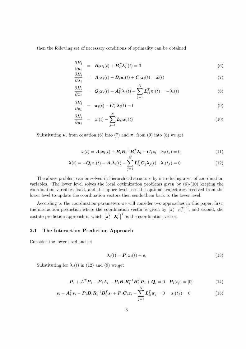
River Pollution Control

The problem for the river pollution control (RPC) is to maintain the instream biomedical oxygendemand (BOD) and the desolved oxygen (DO) at prespecified levels for a river with multiplepolluters using the discharges from the sewage stations as the control variables. The control problemfor a two-reach system without delay is represented by.13

minJ =∫ 8

0(x(t)− xd)T Q(x(t)− xd) + uT (t)Riu(t)dt,

x(t) = Ax(t) + Bu(t) + D, x(0) = xo, (52)

13

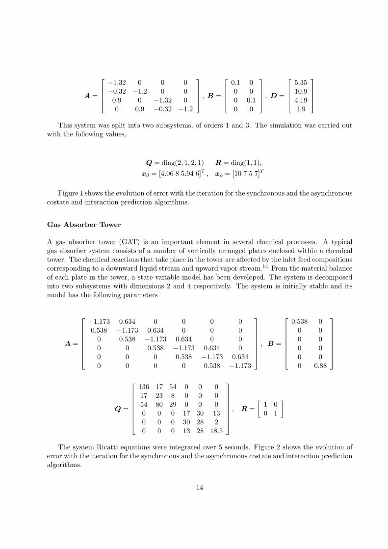
A =

−1.32 0 0 0−0.32 −1.2 0 00.9 0 −1.32 00 0.9 −0.32 −1.2

, B =

0.1 00 00 0.10 0

, D =

5.3510.94.191.9

This system was split into two subsystems, of orders 1 and 3. The simulation was carried outwith the following values,

Q = diag(2, 1, 2, 1) R = diag(1, 1),xd = [4.06 8 5.94 6]T , xo = [10 7 5 7]T

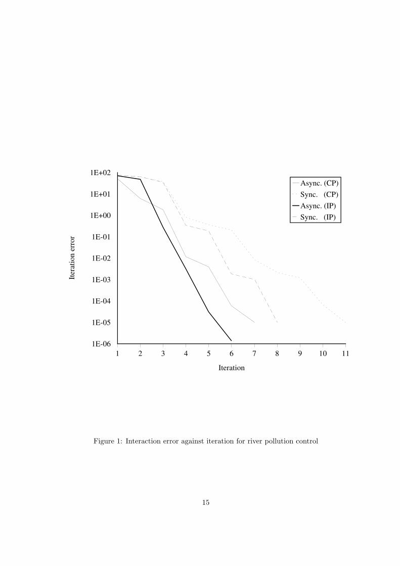
Figure 1 shows the evolution of error with the iteration for the synchronous and the asynchronouscostate and interaction prediction algorithms.

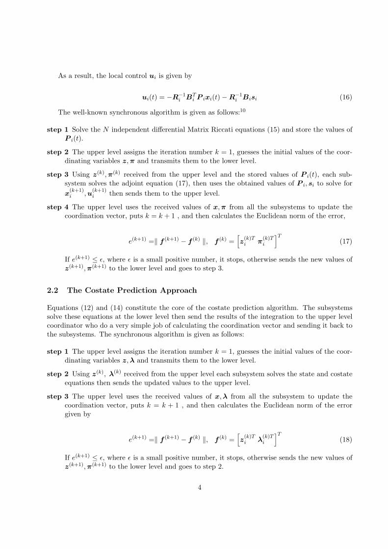
Gas Absorber Tower

A gas absorber tower (GAT) is an important element in several chemical processes. A typicalgas absorber system consists of a number of vertically arranged plates enclosed within a chemicaltower. The chemical reactions that take place in the tower are affected by the inlet feed compositionscorresponding to a downward liquid stream and upward vapor stream.14 From the material balanceof each plate in the tower, a state-variable model has been developed. The system is decomposedinto two subsystems with dimensions 2 and 4 respectively. The system is initially stable and itsmodel has the following parameters

A =

−1.173 0.634 0 0 0 00.538 −1.173 0.634 0 0 0

0 0.538 −1.173 0.634 0 00 0 0.538 −1.173 0.634 00 0 0 0.538 −1.173 0.6340 0 0 0 0.538 −1.173

, B =

0.538 00 00 00 00 00 0.88

Q =

136 17 54 0 0 017 23 8 0 0 054 80 29 0 0 00 0 0 17 30 130 0 0 30 28 20 0 0 13 28 18.5

, R =[

1 00 1

]

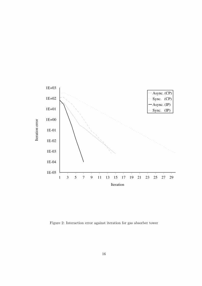
The system Ricatti equations were integrated over 5 seconds. Figure 2 shows the evolution oferror with the iteration for the synchronous and the asynchronous costate and interaction predictionalgorithms.

14

1 2 3 4 5 6 7 8 9 10 11

Iteration

1E-06

1E-05

1E-04

1E-03

1E-02

1E-01

1E+00

1E+01

1E+02

Iter

atio

n e

rro

r

Async. (CP)

Sync. (CP)

Async. (IP)

Sync. (IP)

Figure 1: Interaction error against iteration for river pollution control

15

1 3 5 7 9 11 13 15 17 19 21 23 25 27 29

Iteration

1E-05

1E-04

1E-03

1E-02

1E-01

1E+00

1E+01

1E+02

1E+03

Iter

atio

n e

rro

r

Async. (CP)

Sync. (CP)

Async. (IP)

Sync. (IP)

Figure 2: Interaction error against iteration for gas absorber tower

16

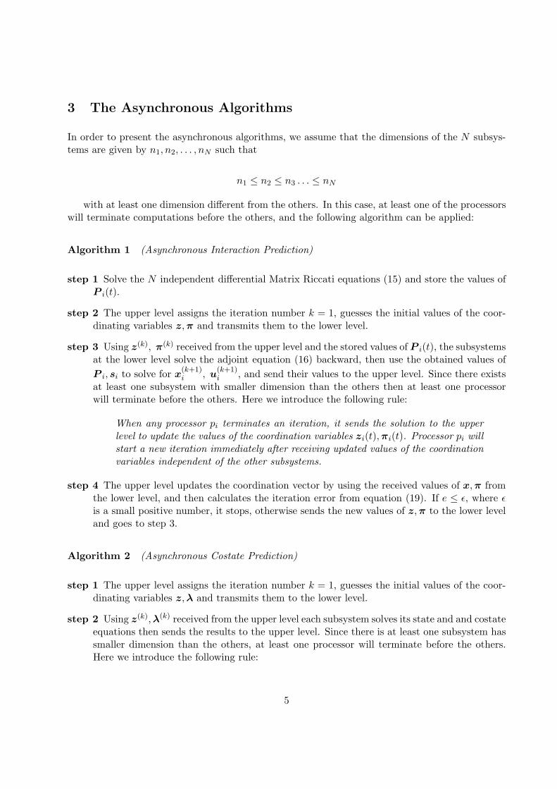
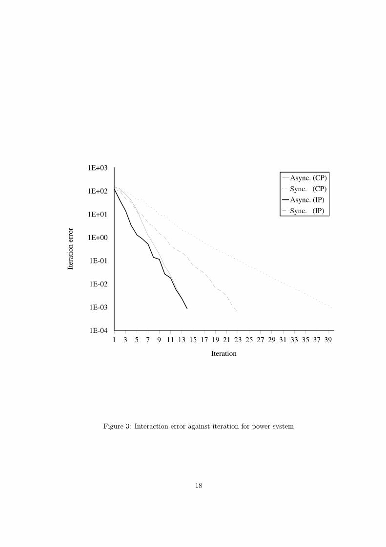
Power System Control

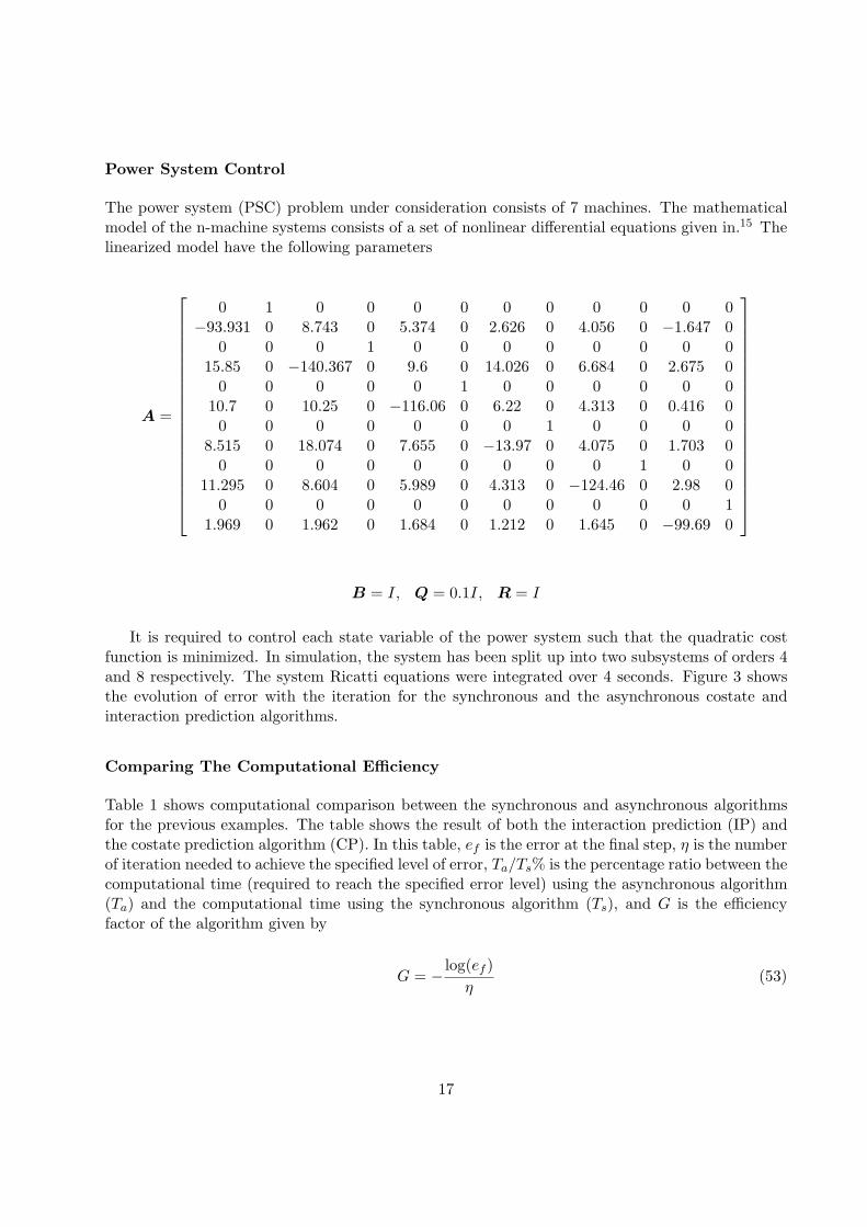
The power system (PSC) problem under consideration consists of 7 machines. The mathematicalmodel of the n-machine systems consists of a set of nonlinear differential equations given in.15 Thelinearized model have the following parameters

A =

0 1 0 0 0 0 0 0 0 0 0 0−93.931 0 8.743 0 5.374 0 2.626 0 4.056 0 −1.647 0

0 0 0 1 0 0 0 0 0 0 0 015.85 0 −140.367 0 9.6 0 14.026 0 6.684 0 2.675 0

0 0 0 0 0 1 0 0 0 0 0 010.7 0 10.25 0 −116.06 0 6.22 0 4.313 0 0.416 00 0 0 0 0 0 0 1 0 0 0 0

8.515 0 18.074 0 7.655 0 −13.97 0 4.075 0 1.703 00 0 0 0 0 0 0 0 0 1 0 0

11.295 0 8.604 0 5.989 0 4.313 0 −124.46 0 2.98 00 0 0 0 0 0 0 0 0 0 0 1

1.969 0 1.962 0 1.684 0 1.212 0 1.645 0 −99.69 0

B = I, Q = 0.1I, R = I

It is required to control each state variable of the power system such that the quadratic costfunction is minimized. In simulation, the system has been split up into two subsystems of orders 4and 8 respectively. The system Ricatti equations were integrated over 4 seconds. Figure 3 showsthe evolution of error with the iteration for the synchronous and the asynchronous costate andinteraction prediction algorithms.

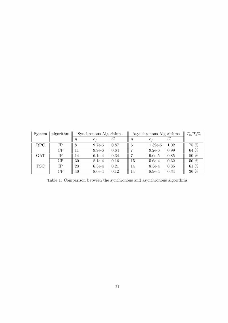
Comparing The Computational Efficiency

Table 1 shows computational comparison between the synchronous and asynchronous algorithmsfor the previous examples. The table shows the result of both the interaction prediction (IP) andthe costate prediction algorithm (CP). In this table, ef is the error at the final step, η is the numberof iteration needed to achieve the specified level of error, Ta/Ts% is the percentage ratio between thecomputational time (required to reach the specified error level) using the asynchronous algorithm(Ta) and the computational time using the synchronous algorithm (Ts), and G is the efficiencyfactor of the algorithm given by

G = − log(ef )η

(53)

17

1 3 5 7 9 11 13 15 17 19 21 23 25 27 29 31 33 35 37 39

Iteration

1E-04

1E-03

1E-02

1E-01

1E+00

1E+01

1E+02

1E+03

Iter

atio

n e

rro

r

Async. (CP)

Sync. (CP)

Async. (IP)

Sync. (IP)

Figure 3: Interaction error against iteration for power system

18

7 Conclusion

In this paper, we proposed asynchronous algorithms for the costate and interaction prediction meth-ods. A mathematical study of the convergence behavior of the proposed algorithms is presented. Itis shown that the new algorithm is convergent under given sufficient conditions which are stronglyrelated to the interaction between the subsystems and the integration period. In the case of thecostate prediction, the internal system structure also influences the convergence of the algorithm.

In view of the structural properties and the convergence results of the proposed algorithms,some important comments related to the practical implementation are presented. Also, we suggestspecific methods to reduce the effect of the high communication delay resulting from excessiveinformation exchange among the subsystems.

Finally, we present the results of the numerical simulation of the algorithms applied to a numberof practical systems. In general, the solutions were identical to the global optimal solution obtainedfrom both the centralized and synchronous algorithms. The comparison with the asynchronousalgorithms shows that a substantial reduction in the total calculation time is achieved through theproposed algorithms for all examined cases.

References

[1] Mahmoud, M. S., M. F. Hassan and M. G. Darwish, Large Scale Control Systems Theoriesand Techniques, Dekkar, New York, 1985.

[2] Bertsekas, D. B. and J. N. Tsitsiklis, ’Some aspects of parallel and distributed iterativealgorithms-a survey’, Automatica, 27, 3–21, (1991).

[3] Kung, H. T., ’Synchronized and asynchronous parallel algorithms for multiprocessors’, In J.F.Traub, editor, Algorithms and complexity :New directions and Recent Results, pages 217–292.Academic Press, (1976).

[4] Bertsekas, D. B. and J. N. Tsitsiklis, Parallel and distributed computation: Numerical Methods,Prentice-Hall, Englewood Cliffs, NJ, 1989.

[5] Lang, B., J. C. Miellou, and P. Spiteri, ’Asynchronous relaxation algorithms for optimal controlproblems’, Mathematics and Computer in Simulation, 28, 227–242, (1986).

[6] Mitra, D., ’Asynchronous relaxation for the numerical solutions of differential equations byparallel processors’, Siam J. Sci. Stat. Comput., 8, s43–58, (1987).

[7] Abdelwahed, S. S., M. F. Hassan, and M. A. Sultan, ’Partially asynchronous co-state predictionalgorithm’, IEE Proc. Control Theory Appl., 142, 88–94, (1995).

[8] Hassan, M. F., ’New multi-level algorithm for linear dynamical systems’, Int. J. Sys. Sci., 19,(1988).

[9] El-Tarazi, M. M., ’Some convergence results for asynchronous algorithms’, Numreish Mathe-matik, 39, 325–340, (1982).

19

[10] Jamshidi, M., Large-scale Systems Modeling and Control, North-Holland, New York, 1983.

[11] Abdelwahed, S. S., Development of multi-level asynchronous algorithms for complex systems,Master’s thesis, Dept. of Elec. Eng., Cairo Univ. Egypt, 1993.

[12] Singh, M. G. and A. Titli, Systems: Decomposition, Optimization, and Control, PergamonPress, Oxford, 1978.

[13] Tamura, H., ’Decentralized optimization for distributed-lag models of discrete systems’, IEEETrans. Sys. Man Cyber., 4, 424–429, (1974).

[14] Darwish, M. and J. Fantin, ’Stabilization and control of absorber tower chemical process’, InThird IFAC/IFIP/IFORs Conf., pages 153–158. Rabat,Moroco, (1970).

[15] Darwish, M. and J. Fantin, ’The application of lyapunov method to large power systems usingdecomposition and aggregation techniques’, Int. J. Control, 29, 351–362, (1979).

20

System algorithm Synchronous Algorithms Asynchronous Algorithms Ta/Ts%η ef G η ef G

RPC IP 8 9.7e-6 0.87 6 1.39e-6 1.02 75 %CP 11 9.9e-6 0.64 7 9.2e-6 0.99 64 %

GAT IP 14 6.1e-4 0.34 7 9.6e-5 0.85 50 %CP 30 8.1e-4 0.16 15 5.6e-4 0.32 50 %

PSC IP 23 6.3e-4 0.21 14 8.3e-4 0.35 61 %CP 40 8.6e-4 0.12 14 8.9e-4 0.34 36 %

Table 1: Comparison between the synchronous and asynchronous algorithms

21