Mechatronics 24 (2014) 98–107

Contents lists available at ScienceDirect

Mechatronics

journal homepage: www.elsevier .com/ locate /mechatronics

Hierarchical optimal contour control of motion systems

0957-4158/$ - see front matter � 2013 Elsevier Ltd. All rights reserved.http://dx.doi.org/10.1016/j.mechatronics.2013.12.007

⇑ Corresponding author. Tel.: +1 573 341 4586.E-mail addresses: hzt42@mst.edu (H. Zomorodi Moghadam), landersr@mst.edu

(R.G. Landers), bala@mst.edu (S.N. Balakrishnan).

Hesam Zomorodi Moghadam, Robert G. Landers ⇑, S.N. BalakrishnanDepartment of Mechanical and Aerospace and Engineering, University of Missouri Science and Technology, Rolla, MO 65409-0050, United States

a r t i c l e i n f o

Article history:Received 25 November 2012Accepted 20 December 2013Available online 22 January 2014

Keywords:Contour controlDiscrete optimal controlHierarchical control

a b s t r a c t

Many motion control applications utilize multiple axes to traverse complex trajectories. The hierarchicalcontour control methodology proposed in this paper treats each axis as an individual subsystem andcombines the Internal Model Principle with robust tracking and optimal hierarchical control techniquesto track a desired trajectory. In this method the objectives are divided into two levels. Measurable goals ofeach subsystem are included in the bottom level and unmeasurable goals, which are estimated using thebottom level states, are considered in the top level where the subsystems are synchronized. The proposedmethodology reduces system complexity while greatly improving tracking performance. The trackingerror for each axis is considered in the bottom level where the Internal Model Principle is used to com-pensate for unmodeled nonlinear friction and slowly varying uncertainties. The top level goal (i.e., zerocontour error) is propagated to the lower level by an aggregation relationship between contour errorand physical linear axis variables. A controller is designed at the bottom level which simultaneously sat-isfies the bottom level goals (i.e., individual axis tracking) and the top level goal. Experimental resultsimplemented on a table top CNC machine for diamond and freeform contours illustrate the performanceof the proposed methodology. While this methodology was implemented for a two-axis motion system, itcan be extended to any motion system containing more than two axes.

� 2013 Elsevier Ltd. All rights reserved.

1. Introduction

Accurate trajectory control is a fundamental requirement inmost motion control applications (e.g., robotics, manufacturing).For many contours multiple axes must be utilized simultaneously.When the independent controllers for each axis are utilized, anydifferences in the performance of one axis caused by disturbances,variation in parameters, etc., in addition to tracking errors, maycause the axes to become unsynchronized. This unsynchronizedmotion produces contour error, which is defined as the closest dis-tance between the current location and the desired path of the mo-tion system. To compensate for axis and contour errors, twodifferent approaches, respectively, have been adopted: trackingcontrol and contour control. In tracking control, feedback controlof individual axes was first utilized; however, since the referenceis usually known, feed forward methods emerged to improvetracking performance. As examples, a velocity feed-forward loopwas used in [1] and Zero Phase Error Tracking Control (ZPETC)was proposed in [2]. In addition to the drawbacks of these tech-niques (e.g., producing high frequency components in the controlsignal and sensitivity to disturbances and variations in parameters)they do not guarantee reduction of contour error, even though they

improve single axis tracking. The literature in this area typicallyconsiders cases where no physical coupling exists between theaxes. To regulate the synchronization error, a virtual coupling be-tween the axes has been introduced using different methods[3,4]. The first such technique was Cross Coupling Control (CCC)proposed by Koren [5]. In CCC methods the contour error is calcu-lated online and a modification to the control law or the referencesignal is generated accordingly. Other methods have introducedvirtual coupling using different approaches such as adaptive cou-pling control [6], fuzzy logic [7], and neural network techniques[8].

Studies in CCC can be divided in two groups by the strategy theyadopt: pre-compensation and control signal manipulation. Severalresearch studies utilized the idea of pre-compensation, which isregulating the contour error by manipulating the axis referencesignals. Freng et al. [9] used CCC to minimize the orientation errorof a differential-drive mobile robot by sending wheel speedcorrection signals. Chin and Lin [10] proposed a Cross-CoupledPre-compensation Method (CCPM) to improve accuracy andeliminate steady-state errors. Lee and Jeon [11] implementedreal-time contour error compensation that calculated the contourerror and modified the reference position commands. In anotherwork Shih et al. [12] combined CCC with a multiple-loop cascadedcontrol design method. Chin et al. [13] improved the performanceof the CCPM by integrating it with a fuzzy logic algorithm. Chenget al. [14] incorporated position feedback, velocity feedforward, a

H. Zomorodi Moghadam et al. / Mechatronics 24 (2014) 98–107 99

fuzzy regulator, and a CCC equipped with a real-time contour errorestimator. Su and Cheng [15] combined position error pre-com-pensation, a modified CCC, and a fuzzy-logic based feedrate regula-tor. In a work by Altinas and Khoshdarregi [16] a vibrationavoidance and contouring error compensation algorithm was pro-posed. In this work a pre-compensation component was generatedfrom the axis closed-loop transfer functions. In order to improvethe contour accuracy, input shaping filters were implemented onthe generated reference positions for vibration avoidance.

Other research studies in CCC used the idea of directly manipu-lating the control signal of each axis. Part of the literature in thisarea used neural networks structure to improve robustness (e.g.,[17]). Other studies have combined various control methods withCCC. Chiu and Tomizuka [18] introduced a coupling effect to eachaxis into a multi-axis system by the proper choice of a Lyapunov-like function. Ho et al. [19] proposed a path following controllerwith decoupled tangential and normal control. Yeh and Hsu [20]combined feedback proportional control and feedforward ZPETCcontrol. A contour error transfer function was then derived to de-sign the integrated controller. In another study Chiu and Tomizuka[21] proposed a method based on a moving coordinate frame at-tached to the desired contour. Chen et al. [22] used an integral slid-ing mode controller based on polar coordinates. In [23] acontouring error vector was estimated to efficiently determinethe variable gains for CCC. A linear CCC was proposed in [24] to im-prove tracking accuracy at high speeds. In another study by Koren[25], a proportional controller, cross coupling controller, and ZPETCwere compared and the effect of their combination in a cross cou-pling formulation was analyzed. McNab and Tsao [26], formulatedthe contour tracking problem as a receding horizon linear qua-dratic problem with variable state weighting matrices. A stabilityproof was provided for linear reference trajectories. In a recentwork by Tang and Landers [27] a model predictive controller wasused to optimally synchronize the subsystems while a pre-com-pensation scheme was used to improve system performance byvarying the feederate according to the predicted contour error.Ouyang et al. [28] proposed a PD contour controller in the positiondomain for a multiaxis system. In their method the motion of theaxes are described by a function where one of the axes is consid-ered to be the master axis. Guo et al. [29] combined quantitativefeedback theory with CCC for coordinating hydraulic motors. Inplaces where friction or other unmodeled effects dominate the sys-tem response, fuzzy logic controllers are more applicable thanother methods [25]. For example, [30] introduced an adaptive fuz-zy controller for a 3 axis system with substantial nonlinear frictionto ensure stability robustness. However, these methods cannotexplicitly account for parametric uncertainties in the formulation.Lee et al. [31] proposed an adaptive method based on a Lyapunovtechnique for contour control in which the motion system frictionand inertia were estimated on line. This method showed animprovement over PD controllers and CCC.

In most of the literature contour control has been investigatedfor two-dimensional applications. However, for many industrialapplications precise motion is required for motion systems withmore than two dimensions. Uchiyama et al. [32] suggested a con-tour controller for three-dimensional machining applications usinga coordinate transformation based method. In another applicationfor five axis machine tools, Sencer and Altintas [33] defined twotypes of contouring errors based on the normal deviation of thetool tip from the reference path, and the normal deviation of thetool axis orientation from the reference orientation using sphericalcoordinates.

Generally, in the studies concerning CCC, there is little attentionpaid to the flexibility of the control structure with respect to theprocess effects. For example, in case of a machining process, atsome instances precise regulation of the contour error might lead

to high control actions and hence higher machining forces which,in turn, might cause tool breakage. Optimal control techniquesare usually incorporated in cross coupling control structure to ad-dress these issues. For example [34], used a weighted quadratic dif-ference between each of the axes in the cost function of an optimalcontrol formulation to account for the asynchronicity of the axes.Also, in [35] two different combinations of contour error and con-trol signals in the cost function were investigated. In these works,to ensure a zero tracking steady state error in straight lines a Pro-portional controller was used for each axis which might result inoscillations in presence of measurement noises. Also in these stud-ies no flexibility is available between the synchronicity control sig-nal and tracking control signal. Therefore the net control signalthat is sent to the motors is not guaranteed to be optimum. Somestudies have considered a combination of control signal, trackingerror, and synchronicity error in centralized optimal control for-mulation to overcome these issues. In [3,4] the asynchronicityproblem of multiple axes has been addressed by a centralized opti-mal controller with a cost function consisting of a combination oftracking error, synchronicity error and, control signal. Howevermodel uncertainties and robustness to noise were not considered.None of these works have proposed a systematic way for introduc-ing different objectives as the synchronizing strategy. For example,when machining a slot along a single axis, position control is veryimportant at the beginning and end of the slot, while force controlin the middle would be desirable to maximize operation productiv-ity. As a result, there is a need for a systematic method to switchemphasis between axis tracking and machining process control.The need was first realized by Ulsoy and Koren [36] who investi-gated the literature in machining control at three levels (i.e., servo,process, and supervisory), and suggested the need of hierarchicalmethods to incorporate all three levels.

Landers and Balakrishnan [37] combined contour and servo-mechanism control using hierarchical optimal control techniques,for a two-axis motion control system. In another work by Tanget al. [38] a hierarchical optimal control methodology was intro-duced that simultaneously regulated machining force processes,contour error, and servomechanism position errors. In these worksan error-space based method proposed by Franklin et al. [39] wasutilized and applied via simulation studies. In this paper, a hierar-chical optimal contour controller is developed using optimal andfeedforward control techniques and applied experimentally. A sta-bility proof of the proposed hierarchical controller is given in theAppendix.

First, a dynamic model of a mini CNC machine is presented. Toachieve robust tracking, the Internal Model Principle is utilized inthe bottom level to compensate for unmodeled friction and otherslowly varying uncertainties. Using a hierarchical structure, thecontour error is propagated to the physical level through an aggre-gation relationship. The top level goal (i.e., zero contour error) isdefined and propagated to the lower level by a linear aggregationrelationship between contour error and the linear axis variables.A linear optimal control problem is then introduced with a costfunction that includes the top and bottom level goals, as well asthe control effort. Different experiments on a tabletop CNC explorethe performance of the proposed methodology. Also a thoroughinvestigation is provided on the effect of increasing or decreasingthe importance of contour error.

2. Hierarchical contour control methodology

The contour control methodology is now derived for two linearaxes, denoted x and y, of a table top CNC machine (Fig. 1). Themethodology, however, is expandable to motion systems withmore than two axes. Assuming the electrical dynamics are much

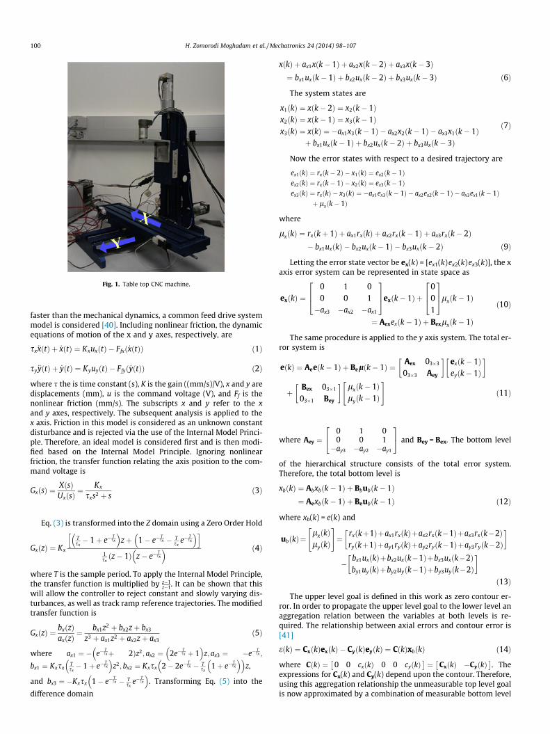
Fig. 1. Table top CNC machine.

100 H. Zomorodi Moghadam et al. / Mechatronics 24 (2014) 98–107

faster than the mechanical dynamics, a common feed drive systemmodel is considered [40]. Including nonlinear friction, the dynamicequations of motion of the x and y axes, respectively, are

sx€xðtÞ þ _xðtÞ ¼ KxuxðtÞ � Ffxð _xðtÞÞ ð1Þ

sy€yðtÞ þ _yðtÞ ¼ KyuyðtÞ � Ffyð _yðtÞÞ ð2Þ

where s the is time constant (s), K is the gain ((mm/s)/V), x and y aredisplacements (mm), u is the command voltage (V), and Ff is thenonlinear friction (mm/s). The subscripts x and y refer to the xand y axes, respectively. The subsequent analysis is applied to thex axis. Friction in this model is considered as an unknown constantdisturbance and is rejected via the use of the Internal Model Princi-ple. Therefore, an ideal model is considered first and is then modi-fied based on the Internal Model Principle. Ignoring nonlinearfriction, the transfer function relating the axis position to the com-mand voltage is

GxðsÞ ¼XðsÞUxðsÞ

¼ Kx

sxs2 þ sð3Þ

Eq. (3) is transformed into the Z domain using a Zero Order Hold

GxðzÞ ¼ Kx

Tsx� 1þ e�

Tsx

� �zþ 1� e�

Tsx � T

sxe�

Tsx

� �h i1sxðz� 1Þ z� e�

Tsx

� � ð4Þ

where T is the sample period. To apply the Internal Model Principle,the transfer function is multiplied by z�1

z�1. It can be shown that thiswill allow the controller to reject constant and slowly varying dis-turbances, as well as track ramp reference trajectories. The modifiedtransfer function is

GxðzÞ ¼bxðzÞaxðzÞ

¼ bx1z2 þ bx2zþ bx3

z3 þ ax1z2 þ ax2zþ ax3ð5Þ

where ax1 ¼ � e�Tsxþ

�2Þz2; ax2 ¼ 2e�

Tsx þ 1

� �z; ax3 ¼ �e�

Tsx ;

bx1 ¼ KxsxTsx� 1þ e�

Tsx

� �z2; bx2 ¼ Kxsx 2� 2e�

Tsx � T

sx1þ e�

Tsx

� �� �z,

and bx3 ¼ �Kxsx 1� e�Tsx � T

sxe�

Tsx

� �. Transforming Eq. (5) into the

difference domain

xðkÞ þ ax1xðk� 1Þ þ ax2xðk� 2Þ þ ax3xðk� 3Þ¼ bx1uxðk� 1Þ þ bx2uxðk� 2Þ þ bx3uxðk� 3Þ ð6Þ

The system states are

x1ðkÞ ¼ xðk� 2Þ ¼ x2ðk� 1Þx2ðkÞ ¼ xðk� 1Þ ¼ x3ðk� 1Þx3ðkÞ ¼ xðkÞ ¼ �ax1x3ðk� 1Þ � ax2x2ðk� 1Þ � ax3x1ðk� 1Þ

þ bx1uxðk� 1Þ þ bx2uxðk� 2Þ þ bx3uxðk� 3Þ

ð7Þ

Now the error states with respect to a desired trajectory are

ex1ðkÞ ¼ rxðk� 2Þ � x1ðkÞ ¼ ex2ðk� 1Þex2ðkÞ ¼ rxðk� 1Þ � x2ðkÞ ¼ ex3ðk� 1Þex3ðkÞ ¼ rxðkÞ � x3ðkÞ ¼ �ax1ex3ðk� 1Þ � ax2ex2ðk� 1Þ � ax3ex1ðk� 1Þ

þ lxðk� 1Þ

where

lxðkÞ ¼ rxðkþ 1Þ þ ax1rxðkÞ þ ax2rxðk� 1Þ þ ax3rxðk� 2Þ� bx1uxðkÞ � bx2uxðk� 1Þ � bx3uxðk� 2Þ ð9Þ

Letting the error state vector be ex(k) = [ex1(k)ex2(k)ex3(k)], the xaxis error system can be represented in state space as

exðkÞ ¼0 1 00 0 1�ax3 �ax2 �ax1

264

375exðk� 1Þ þ

001

264

375lxðk� 1Þ

¼ Aexexðk� 1Þ þ Bexlxðk� 1Þ

ð10Þ

The same procedure is applied to the y axis system. The total er-ror system is

eðkÞ ¼ Aeeðk� 1Þ þ Belðk� 1Þ ¼Aex 03�3

03�3 Aey

� �exðk� 1Þeyðk� 1Þ

� �

þBex 03�1

03�1 Bey

� � lxðk� 1Þlyðk� 1Þ

" #ð11Þ

where Aey ¼0 1 00 0 1�ay3 �ay2 �ay1

24

35 and Bey = Bex. The bottom level

of the hierarchical structure consists of the total error system.Therefore, the total bottom level is

xbðkÞ ¼ Abxbðk� 1Þ þ Bbubðk� 1Þ¼ Aexbðk� 1Þ þ Beubðk� 1Þ ð12Þ

where xb(k) = e(k) and

ubðkÞ¼lxðkÞlyðkÞ

" #¼

rxðkþ1Þþax1rxðkÞþax2rxðk�1Þþax3rxðk�2Þryðkþ1Þþay1ryðkÞþay2ryðk�1Þþay3ryðk�2Þ

� �

�bx1uxðkÞþbx2uxðk�1Þþbx3uxðk�2Þby1uyðkÞþby2uyðk�1Þþby3uyðk�2Þ

� �ð13Þ

The upper level goal is defined in this work as zero contour er-ror. In order to propagate the upper level goal to the lower level anaggregation relation between the variables at both levels is re-quired. The relationship between axial errors and contour error is[41]

eðkÞ ¼ CxðkÞexðkÞ � CyðkÞeyðkÞ ¼ CðkÞxbðkÞ ð14Þ

where CðkÞ ¼ 0 0 cxðkÞ 0 0 cyðkÞ� �

¼ CxðkÞ �CyðkÞ� �

. Theexpressions for Cx(k) and Cy(k) depend upon the contour. Therefore,using this aggregation relationship the unmeasurable top level goalis now approximated by a combination of measurable bottom level

H. Zomorodi Moghadam et al. / Mechatronics 24 (2014) 98–107 101

states. As can be seen in Eq. (14), the top level error automaticallygoes to zero if the bottom level errors are driven to zero. However,bottom level errors are unavoidable during transient phases. It willbe seen that emphasizing contour error will allow the axes to becoordinated such that contour error is reduced even during thesephases. At these points top and bottom goals are competing objec-tives and it is desirable for both to be small. In fact, the bottom levelgoal results in preventing the deviation of each axis from its refer-ence and the top level goal synchronizes the axes and ensures therelative movement of the axes which results in a trajectory closerto the desired trajectory.

The next step is to formulate and solve an optimal tracking con-trol problem as outlined in [42] with a modified cost function. Atthis point the top level goal is approximated using the aggregationrelationship and included in the cost function

Jb ¼12

X1k¼1

LbðkÞ ð15Þ

where

LbðkÞ ¼12

�½CðkÞxbðkÞ � erðkÞ�T q½CðkÞxbðkÞ � erðkÞ� þ uT

bðkÞRbubðkÞ

þxTbðkÞQ bxbðkÞ

ð16Þ

and er is the reference contour error, which is zero. In Eq. (16) thefirst term maintains the aggregation relationship between the topand bottom levels. The second and third terms are used to penalizethe control usage and state deviations, respectively, at the bottomlevel. The Hamiltonian at the bottom level is

HbðkÞ ¼ LbðkÞ þ kTbðkþ 1Þ½AbxbðkÞ þ BbubðkÞ� ð17Þ

Taking the derivative of the Hamiltonian with respect to xB(k)and setting er(k) = 0, the Lagrange multiplier is

kbðkÞ ¼ ½CTðkÞqCðkÞ þ Q b�xbðkÞ þ ATbkbðkþ 1Þ ð18Þ

Taking the partial derivative of Eq. (17) with respect to ub(k),equating the result to zero, and rearranging gives the optimal con-trol law

ubðkÞ ¼ �R�1b BT

bkbðkþ 1Þ ð19Þ

Substituting ub(k) from Eq. (19) into Eq. (12) results in

Fig. 2. Block diagram of th

xbðkþ 1Þ ¼ AbxbðkÞ � BbR�1b BT

bkbðkþ 1Þ ð20Þ

Now it is assumed that the Lagrangian multiplier can be ex-pressed as

kbðkÞ ¼ PbðkÞxbðkÞ ð21Þ

where Pb(k) is a positive definite, nonsingular matrix. SubstitutingEq. (21) into Eqs. (18) and (20) and rearranging, the followingRicatti equation is derived

PbðkÞ ¼ CTðkÞqCðkÞ þ Q b þ ATbPbðk

þ 1ÞðIþ BbR�1b BT

bPbðkþ 1ÞÞ�1Ab ð22Þ

The matrix Pb(k) is found from solving Eq. (22). As shown in thecost function in Eq. (15), an infinite horizon optimal control formu-lation is used to find the optimal signal ub(k). Therefore, the steadystate value of Pb(k), denoted Pb; is used to solve the above Ricattiequation. Given Ab, Bb, Qb, Rb, q, and C(k), the term Pb can be cal-culated off-line. If the ranges of variations in cx and cy are known,curves can be fit to the entries of Pb over the cx and cy ranges. Thesecurves are then used for online implementation to increase compu-tational efficiency. Knowing the time history of Pb, the optimalcontrol signal can be expressed as

ubðkÞ ¼ �KbxbðkÞ ð23Þ

where the control gain is

Kb ¼ ½Rb þ BTbPbBb�

�1BT

bPbAb ð24Þ

The physical control signals are found by solving the followingequation for ux(k) and uy(k)

bx1uxðkÞby1uyðkÞ

� �¼

rxðkþ1Þþax1rxðkÞþax2rxðk�1Þþax3rxðk�2Þryðkþ1Þþay1ryðkÞþay2ryðk�1Þþay3ryðk�2Þ

� �

þKbxbðkÞ�bx2uxðk�1Þþbx3uxðk�2Þby2uyðk�1Þþby3uyðk�2Þ

� � ð25Þ

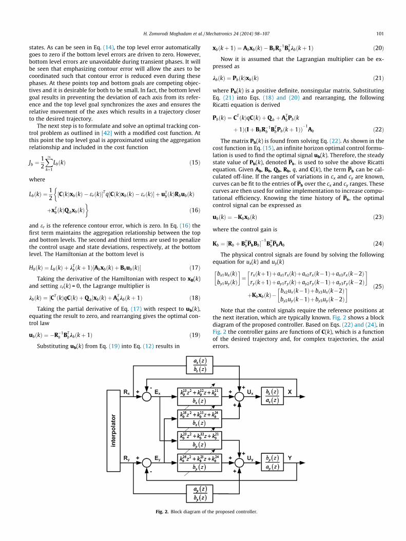
Note that the control signals require the reference positions atthe next iteration, which are typically known. Fig. 2 shows a blockdiagram of the proposed controller. Based on Eqs. (22) and (24), inFig. 2 the controller gains are functions of C(k), which is a functionof the desired trajectory and, for complex trajectories, the axialerrors.

e proposed controller.

0 5 10 15 20 25

-10

-5

0

5

10

15

X [mm]

Y [m

m]

Start point

20o

Fig. 3. Diamond contour schematic.

10-2 10-1 100 101 1020

20

40

60

80

100

q/qb

max

(err

or) [

μm]

exeyε

Fig. 4. Maximum transient errors for Cases I–V.

ith desired reference point

ith real point with low contour emphasis

ith real point with high contour emphasis

line connecting the corresponding real points

line connecting the reference point to the real points

desired path

102 H. Zomorodi Moghadam et al. / Mechatronics 24 (2014) 98–107

3. Experimental results and discussion

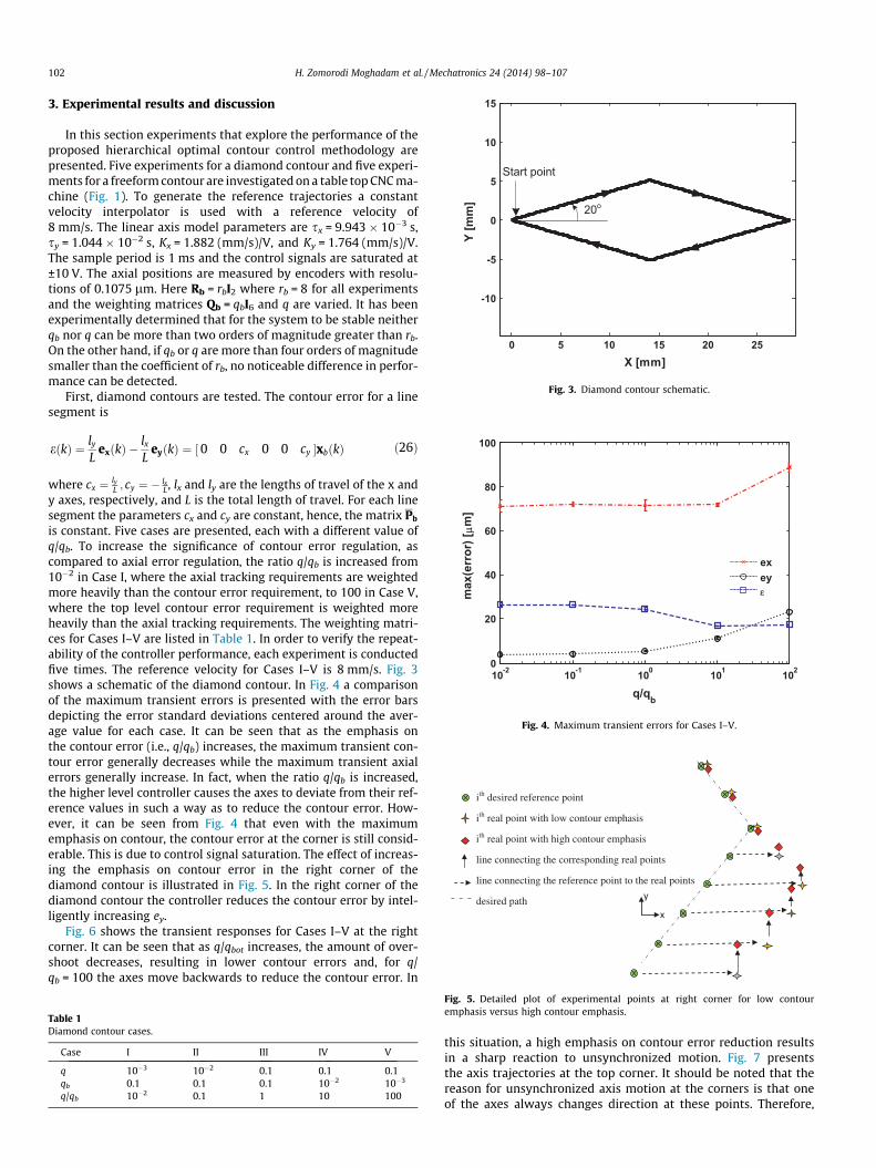
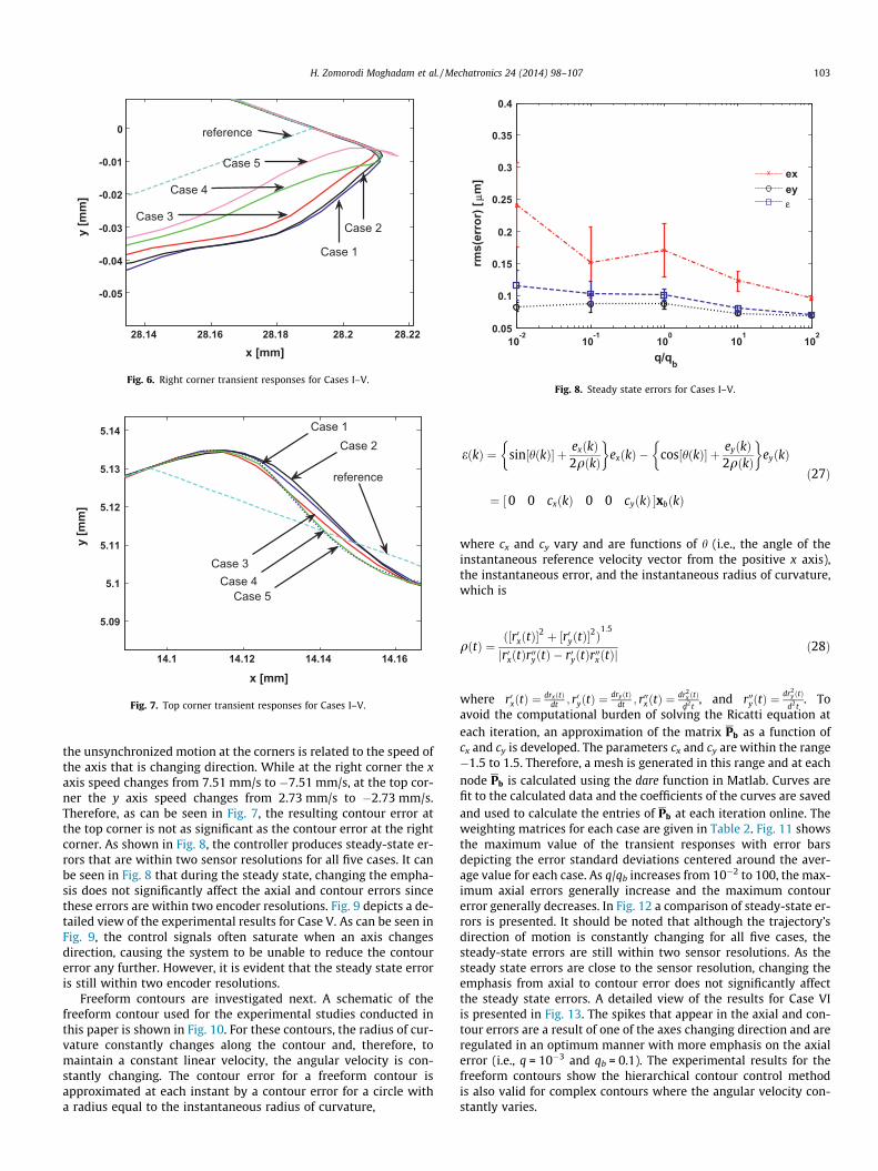
In this section experiments that explore the performance of theproposed hierarchical optimal contour control methodology arepresented. Five experiments for a diamond contour and five experi-ments for a freeform contour are investigated on a table top CNC ma-chine (Fig. 1). To generate the reference trajectories a constantvelocity interpolator is used with a reference velocity of8 mm/s. The linear axis model parameters are sx = 9.943 � 10�3 s,sy = 1.044 � 10�2 s, Kx = 1.882 (mm/s)/V, and Ky = 1.764 (mm/s)/V.The sample period is 1 ms and the control signals are saturated at±10 V. The axial positions are measured by encoders with resolu-tions of 0.1075 lm. Here Rb = rbI2 where rb = 8 for all experimentsand the weighting matrices Qb = qbI6 and q are varied. It has beenexperimentally determined that for the system to be stable neitherqb nor q can be more than two orders of magnitude greater than rb.On the other hand, if qb or q are more than four orders of magnitudesmaller than the coefficient of rb, no noticeable difference in perfor-mance can be detected.

First, diamond contours are tested. The contour error for a linesegment is

eðkÞ ¼ ly

LexðkÞ �

lx

LeyðkÞ ¼ 0 0 cx 0 0 cy½ �xbðkÞ ð26Þ

where cx ¼ lyL ; cy ¼ � lx

L , lx and ly are the lengths of travel of the x andy axes, respectively, and L is the total length of travel. For each linesegment the parameters cx and cy are constant, hence, the matrix Pb

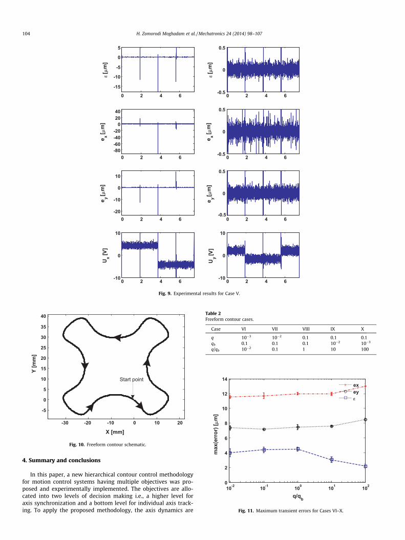
is constant. Five cases are presented, each with a different value ofq/qb. To increase the significance of contour error regulation, ascompared to axial error regulation, the ratio q/qb is increased from10�2 in Case I, where the axial tracking requirements are weightedmore heavily than the contour error requirement, to 100 in Case V,where the top level contour error requirement is weighted moreheavily than the axial tracking requirements. The weighting matri-ces for Cases I–V are listed in Table 1. In order to verify the repeat-ability of the controller performance, each experiment is conductedfive times. The reference velocity for Cases I–V is 8 mm/s. Fig. 3shows a schematic of the diamond contour. In Fig. 4 a comparisonof the maximum transient errors is presented with the error barsdepicting the error standard deviations centered around the aver-age value for each case. It can be seen that as the emphasis onthe contour error (i.e., q/qb) increases, the maximum transient con-tour error generally decreases while the maximum transient axialerrors generally increase. In fact, when the ratio q/qb is increased,the higher level controller causes the axes to deviate from their ref-erence values in such a way as to reduce the contour error. How-ever, it can be seen from Fig. 4 that even with the maximumemphasis on contour, the contour error at the corner is still consid-erable. This is due to control signal saturation. The effect of increas-ing the emphasis on contour error in the right corner of thediamond contour is illustrated in Fig. 5. In the right corner of thediamond contour the controller reduces the contour error by intel-ligently increasing ey.

Fig. 6 shows the transient responses for Cases I–V at the rightcorner. It can be seen that as q/qbot increases, the amount of over-shoot decreases, resulting in lower contour errors and, for q/qb = 100 the axes move backwards to reduce the contour error. In

Fig. 5. Detailed plot of experimental points at right corner for low contouremphasis versus high contour emphasis.

Table 1Diamond contour cases.

Case I II III IV V

q 10�3 10�2 0.1 0.1 0.1qb 0.1 0.1 0.1 10�2 10�3

q/qb 10�2 0.1 1 10 100

this situation, a high emphasis on contour error reduction resultsin a sharp reaction to unsynchronized motion. Fig. 7 presentsthe axis trajectories at the top corner. It should be noted that thereason for unsynchronized axis motion at the corners is that oneof the axes always changes direction at these points. Therefore,

10-2

10-1

100

101

102

0.05

0.1

0.15

0.2

0.25

0.3

0.35

0.4

q/qb

rms(

erro

r) [

μm] ex

eyε

Fig. 8. Steady state errors for Cases I–V.

14.1 14.12 14.14 14.16

5.09

5.1

5.11

5.12

5.13

5.14

y [m

m]

x [mm]

reference

Case 1Case 2

Case 3Case 4

Case 5

Fig. 7. Top corner transient responses for Cases I–V.

28.14 28.16 28.18 28.2 28.22

-0.05

-0.04

-0.03

-0.02

-0.01

0

y [m

m]

x [mm]

Case 3

Case 4

Case 5

reference

Case 1

Case 2

Fig. 6. Right corner transient responses for Cases I–V.

H. Zomorodi Moghadam et al. / Mechatronics 24 (2014) 98–107 103

the unsynchronized motion at the corners is related to the speed ofthe axis that is changing direction. While at the right corner the xaxis speed changes from 7.51 mm/s to �7.51 mm/s, at the top cor-ner the y axis speed changes from 2.73 mm/s to �2.73 mm/s.Therefore, as can be seen in Fig. 7, the resulting contour error atthe top corner is not as significant as the contour error at the rightcorner. As shown in Fig. 8, the controller produces steady-state er-rors that are within two sensor resolutions for all five cases. It canbe seen in Fig. 8 that during the steady state, changing the empha-sis does not significantly affect the axial and contour errors sincethese errors are within two encoder resolutions. Fig. 9 depicts a de-tailed view of the experimental results for Case V. As can be seen inFig. 9, the control signals often saturate when an axis changesdirection, causing the system to be unable to reduce the contourerror any further. However, it is evident that the steady state erroris still within two encoder resolutions.

Freeform contours are investigated next. A schematic of thefreeform contour used for the experimental studies conducted inthis paper is shown in Fig. 10. For these contours, the radius of cur-vature constantly changes along the contour and, therefore, tomaintain a constant linear velocity, the angular velocity is con-stantly changing. The contour error for a freeform contour isapproximated at each instant by a contour error for a circle witha radius equal to the instantaneous radius of curvature,

eðkÞ ¼ sin½hðkÞ� þ exðkÞ2qðkÞ

� exðkÞ � cos½hðkÞ� þ eyðkÞ

2qðkÞ

� eyðkÞ

¼ ½0 0 cxðkÞ 0 0 cyðkÞ �xbðkÞ

ð27Þ

where cx and cy vary and are functions of h (i.e., the angle of theinstantaneous reference velocity vector from the positive x axis),the instantaneous error, and the instantaneous radius of curvature,which is

qðtÞ ¼ð½r0xðtÞ�

2 þ ½r0yðtÞ�2Þ

1:5

jr0xðtÞr00yðtÞ � r0yðtÞr00xðtÞjð28Þ

where r0xðtÞ ¼drxðtÞ

dt ; r0yðtÞ ¼dryðtÞ

dt ; r00xðtÞ ¼dr2

x ðtÞd2t

, and r00yðtÞ ¼dr2

y ðtÞd2t

. Toavoid the computational burden of solving the Ricatti equation ateach iteration, an approximation of the matrix Pb as a function ofcx and cy is developed. The parameters cx and cy are within the range�1.5 to 1.5. Therefore, a mesh is generated in this range and at eachnode Pb is calculated using the dare function in Matlab. Curves arefit to the calculated data and the coefficients of the curves are savedand used to calculate the entries of Pb at each iteration online. Theweighting matrices for each case are given in Table 2. Fig. 11 showsthe maximum value of the transient responses with error barsdepicting the error standard deviations centered around the aver-age value for each case. As q/qb increases from 10�2 to 100, the max-imum axial errors generally increase and the maximum contourerror generally decreases. In Fig. 12 a comparison of steady-state er-rors is presented. It should be noted that although the trajectory’sdirection of motion is constantly changing for all five cases, thesteady-state errors are still within two sensor resolutions. As thesteady state errors are close to the sensor resolution, changing theemphasis from axial to contour error does not significantly affectthe steady state errors. A detailed view of the results for Case VIis presented in Fig. 13. The spikes that appear in the axial and con-tour errors are a result of one of the axes changing direction and areregulated in an optimum manner with more emphasis on the axialerror (i.e., q = 10�3 and qb = 0.1). The experimental results for thefreeform contours show the hierarchical contour control methodis also valid for complex contours where the angular velocity con-stantly varies.

10-2 10-1 100 101 1020

2

4

6

8

10

12

14

q/qb

max

(err

or) [

μm]

exeyε

Fig. 11. Maximum transient errors for Cases VI–X.

-30 -20 -10 0 10 20

-5

0

5

10

15

20

25

30

35

40

X [mm]

Y [m

m]

Start point

Fig. 10. Freeform contour schematic.

Table 2Freeform contour cases.

Case VI VII VIII IX X

q 10�3 10�2 0.1 0.1 0.1qb 0.1 0.1 0.1 10�2 10�3

q/qb 10�2 0.1 1 10 100

0 2 4 6

-15

-10

-5

0

5

ε [μm

]0 2 4 6-0.5

0

0.5

ε [μm

]

0 2 4 6-80-60-40-20

02040

e x [ μm

]

0 2 4 6-0.5

0

0.5

e x [ μm

]

0 2 4 6-20

-10

0

10

e y [ μm

]

0 2 4 6-0.5

0

0.5

e y [ μm

]

0 2 4 6-10

0

10

U x [V]

0 2 4 6-10

0

10

Uy [V

]

Fig. 9. Experimental results for Case V.

104 H. Zomorodi Moghadam et al. / Mechatronics 24 (2014) 98–107

4. Summary and conclusions

In this paper, a new hierarchical contour control methodologyfor motion control systems having multiple objectives was pro-posed and experimentally implemented. The objectives are allo-cated into two levels of decision making i.e., a higher level foraxis synchronization and a bottom level for individual axis track-ing. To apply the proposed methodology, the axis dynamics are

10-2

10-1

100

101

102

0.06

0.08

0.1

0.12

0.14

0.16

0.18

0.2

0.22

q/qb

rms(

erro

r) [ μ

m]

exeyε

Fig. 12. Steady state errors for Cases VI–X.

H. Zomorodi Moghadam et al. / Mechatronics 24 (2014) 98–107 105

converted into the error domain and the Internal Model Principle,coupled with optimal control, is used to simultaneously satisfy thetop level goal (i.e., zero contour error) and the bottom level goals(i.e., zero axial errors and minimal control usage). The top level

0 5 10 15-10

0

10

u x [V]

0 5 10 15-5

0

5

ε [ μ

m]

0 5 10 15-20

0

20

e x [ μm

]

0 5 10 15-10

0

10

time [s]

e y [ μm

]

Fig. 13. Experimental r

goal is propagated to the physical linear axis level by an aggrega-tion relationship. Optimal control techniques are used to weightthe relative importance between axial and contour errors.

Experimental results on a table top CNC machine demonstratethe excellent tracking capability of this method for diamond andfreeform contours. For both contours, the steady state errors areapproximately 0.2 lm, which are within two encoder resolutions,indicating the excellent tracking and disturbance rejection capabil-ities of the controller. To test the performance of the controller fordifferent relative weightings of the top and bottom level goals, fivecases were conducted, where q/qbot increased from 10�2 (i.e., highweight on axial errors) to 100 (i.e., high weight on contour error). Itwas found that the transient errors generally decreased when thecontour error was weighted more heavily than the axial errorsfor both contours. On the other hand, the steady state errors wereindependent of the relative weighting. This is due to the fact thatfor both cases the steady state error was within two encoder reso-lutions. Two axes of a table top CNC machine was used in this pa-per as a test bed to experimentally implement and analyze theproposed methodology. However, the hierarchical optimal contourcontrol methodology can be extended to any motion system withmultiple axes whose motion must be coordinated. To extend themethodology to more than two axes, a new contour error formula-tion and possibly tool orientation error formulation would need tobe driven and the error dynamics of the additional axes wouldneed to be incorporated.

0 5 10 15-10

0

10

u y [V]

0 5 10 15-0.5

0

0.5

ε [ μ

m]

0 5 10 15-0.5

0

0.5

e x [ μm

]

0 5 10 15-0.5

0

0.5

time [s]

e y [ μm

]

esults for Case VI.

106 H. Zomorodi Moghadam et al. / Mechatronics 24 (2014) 98–107

Acknowledgement

The authors wish to acknowledge the financial support for thiswork from the Intelligent Systems Center at the MissouriUniversity of Science and Technology.

Appendix A. Stability proof of proposed controller

In order to investigate the global asymptotic tracking stabilityof the closed-loop system, the following Lyapunov function candi-date is considered

VðxBðkÞÞ ¼ xTBðkÞPbðkÞxbðkÞ ð29Þ

where V(0) = 0 and PbðkÞ ¼ PbðCðkÞÞ is the steady state solution ofthe Riccati equation. Because PbðkÞ is a positive definite matrix,"xb(k) – 0, V(xb(k)) > 0. The first order forward difference ofV(xb(k)) is

DVðkÞ ¼ Vðxbðkþ 1ÞÞ � VðxbðkÞÞ¼ xT

bðkþ 1ÞPbðkÞxbðkþ 1Þ � xTbðkÞPbðkÞxbðkÞ ð30Þ

Evaluating DV (k) along the error system equation

DVðkÞ ¼ ½AbxbðkÞ þ BbubðkÞ�T PbðkÞ½AbxbðkÞ þ BbubðkÞ�� xT

bðkÞPbðkÞxbðkÞ ð31Þ

Expanding Eq. (31)

DV ¼ xTbðkÞA

TbPbðkþ 1ÞAbxbðkÞ � xT

bðkÞPbðkÞxbðkÞ

þ xTbðkÞA

TbPbðkþ 1ÞBbubðkÞ þ uT

bðkÞBTbPbðkþ 1ÞAbxbðkÞ

þ uTbðkÞB

TbPbðkþ 1ÞBbubðkÞ ð32Þ

Since PbðkÞ is symmetric andxT

bðkÞATbPbðkþ 1ÞBbubðkÞ

h iT¼ uT

bðkÞBTbPbðkþ 1ÞAbxbðkÞ, Eq. (32) can

be rewritten as

DV ¼ xTbðkÞA

TbPbðkþ 1ÞAbxbðkÞ � xT

bðkÞPbðkÞxbðkÞ

þ 2xTbðkÞA

TbPbðkþ 1ÞBbubðkÞ þ uT

bðkÞBTbPbðk

þ 1ÞBbubðkÞ ð33Þ

In order to simplify Eq. (33) the matrix inversion lemma [42] isimplemented to the steady state version of Eq. (22)

PbðkÞ ¼ Q ðkÞ þ ATbPbðkÞAb

� ATbPbðkÞBbðBT

bPbðkÞBb þ RbÞ�1

BTbPbðkÞAb ð34Þ

where Q(k) = CT(k)qC(k) + Qb. Substituting Eq. (34) into the secondterm of Eq. (33) and simplifying

DV ¼ xTbðkÞA

TbPbðkÞBbðUðkÞÞ�1BT

bPbðkÞAbxbðkÞ

� xTbðkÞQ ðkÞxbðkÞ þ xT

bðkÞATb½Pbðkþ 1Þ � PbðkÞ�AbxbðkÞ

þ 2xTbðkÞA

TbPbðkþ 1ÞBbubðkÞ þ uT

bðkÞBTbPbðk

þ 1ÞBbubðkÞ ð35Þ

where UðkÞ ¼ BTBPbðkÞBB þ RB, which is symmetric and nonsingular.

From Eqs. (23) and (24) the control signal can be written as

ubðkÞ ¼ �ðUðkÞÞ�1BTbPbðkÞAbxbðkÞ ð36Þ

Substituting Eq. (36) into the fourth and fifth terms of Eq. (35)and simplifying

DV ¼ �xTbðkÞ �AT

bPbðkÞBbðUðkÞÞ�1BTbPbðkþ 1ÞBbðUðkÞÞ�1BT

bPbðkÞAb

h�AT

b½PbðkÞ � 2Pbðkþ 1Þ�BbðUðkÞÞ�1BTbPbðkÞAb � AT

b½Pbðkþ 1Þ�PbðkÞ�Ab þ Q ðkÞ

�xbðkÞ ð37Þ

Therefore, DV is negative definite when the matrix

M ¼ �ATbPbðkÞBbðUðkÞÞ�1BT

bPbðkþ 1ÞBbðUðkÞÞ�1BTbPbðkÞAb

� ATb½PbðkÞ � 2Pbðkþ 1Þ�BbðUðkÞÞ�1BT

bPbðkÞAb � ATb½Pbðkþ 1Þ

� PbðkÞ�Ab þ Q ðkÞ

is positive definite, which indicates the system is asymptoticallystable. Further, since "xb(k) e Rn, if kxb(k)k?1, V(xb(k)) ?1, thesystem will be globally asymptotically stable. Therefore, for com-plex contours (i.e., contours other than straight lines) the designermust ensure M is positive definite for the expected range of C.When tracking a straight line PbðkÞ ¼ Pb;UðkÞ ¼ U;Q ðkÞ ¼ Q , and

DV ¼ �xTbðkÞ �AT

bPbBbU�1BT

bPbBbU�1BT

bPbAb

hþAT

bPbBbU�1BT

bPbAb þ QixbðkÞ ð38Þ

Substituting Eq. (36) into Eq. (38) and combining the first andsecond terms

DV ¼ �xTbðkÞQxbðkÞ � uT

bðkÞRbubðkÞ < 0 8xbðkÞ–0 ð39Þ

Therefore, when tracking straight lines DV is always negativedefinite and, since "xb(k) e Rn, if kxb(k)k?1, V(xb(k)) ?1, thesystem is always globally asymptotically stable.

References

[1] Masory O. Improving contouring accuracy of NC/CNC systems with additionalvelocity feed forward loop. J Manuf Sci Eng 1986;108(3):227–30.

[2] Tomizuka M. Zero phase error tracking algorithm for digital control. J Dyn SystMeas Control 1987;109(1):65–8.

[3] Cheng MH, Chen CY, Bakhoum EG. Synchronization controller synthesis withthe consideration of multi-resolution. Int J Innovative Comput Inform Control2011;7(7B):1025–30.

[4] Xiao Y, Zhu K, Choo Liaw H. Generalized synchronization control of multi-axismotion systems. Control Eng Pract 2005;13(7):809–19.

[5] Koren Y. Cross-coupled biaxial computer control for manufacturing systems.ASME J Dyn Syst Meas Control 1980;102(4):265–72.

[6] Sun D. Position synchronization of multiple motion axes with adaptivecoupling control. Automatica 2003;39(6):997–1005.

[7] Moore P, Chen C. Fuzzy logic coupling and synchronised control of multipleindependent servo-drives. Control Eng Pract 1995;3(12):1697–708.

[8] Lee HC, Jeon GJ. A neuro controller for synchronization of two motion axes. IntJ Intell Syst 1998;13(6):571–86.

[9] Feng L, Koren Y, Borenstein J. Cross-coupling motion controller for mobilerobots. IEEE Control Syst Mag 1993;13(6):35–43.

[10] Chin JH, Lin TC. Cross-coupled precompensation method for the contouringaccuracy of computer numerically controlled machine tools. Int J Mach ToolsManuf 1997;37(7):947–67.

[11] Lee HC, Jeon GJ. Real-time compensation of two-dimensional contour error inCNC machine tools. In: IEEE/ASME international conference on advancedintelligent mechatronics. Atlanta, Georgia; 1999. p. 623–8.

[12] Shih Y-T, Chen C-S, Lee A-C. A novel cross-coupling control design for bi-axismotion. Int J Mach Tools Manuf 2002;42(14):1539–48.

[13] Chin JH, Cheng YM, Lin JH. Improving contour accuracy by fuzzy-logicenhanced cross-coupled precompensation method. Rob Comput-IntegrManuf 2004;20(1):65–76.

[14] Cheng MY, Su KH, Wang SF. Contour error reduction for free-form contourfollowing tasks of biaxial motion control systems. Rob Comput-Integr Manuf2009;25(2):323–33.

[15] Su KH, Cheng MY. Contouring accuracy improvement using cross-coupledcontrol and position error compensator. Int J Mach Tools Manuf 2008;48(12–13):1444–53.

[16] Altintas Y, Khoshdarregi M. Contour error control of CNC machine tools withvibration avoidance. In: CIRP annals-manufacturing technology; 2012.

[17] Goto S, Nakamura M, Kyura N. Accurate contour control of mechatronic servosystems using Gaussian networks. IEEE Trans Industr Electron1996;43(4):469–76.

[18] Chiu GTC, Tomizuka M. Coordinated position control of multi-axis mechanicalsystems. ASME J Dyn Syst Meas Control 1998;120(3):389–93.

[19] Ho HC, Yen JY, Lu SS. A decoupled path-following control algorithm basedupon the decomposed trajectory error. Int J Mach Tools Manuf1999;39(10):1619–30.

[20] Yeh S-S, Hsu P-L. Design of precise multi-axis motion control systems. In: 6thInternational workshop on advanced motion control. Nagoya, Japan; 2000. p.234–9.

H. Zomorodi Moghadam et al. / Mechatronics 24 (2014) 98–107 107

[21] Chiu GTC, Tomizuka M. Contouring control of machine tool feed drive systems:a task coordinate frame approach. IEEE Trans Control Syst Technol2001;9(1):130–9.

[22] Chen SL, Liu HL, Ting SC. Contouring control of biaxial systems based on polarcoordinates. IEEE/ASME Trans Mechatron 2002;7(3):329–45.

[23] Yeh SS, Hsu PL. Estimation of the contouring error vector for the cross-coupledcontrol design. IEEE/ASME Trans Mechatron 2002;7(1):44–51.

[24] Zhong Q, Shi Y, Mo J, Huang S. A linear cross-coupled control system for high-speed machining. Int J Adv Manuf Technol 2002;19(8):558–63.

[25] Koren Y. Control of machine tools. ASME J Mech Des 1997;119:749–55.[26] McNab RJ, Tsao T-C. Receding time horizon linear quadratic optimal control for

multi-axis contour tracking motion control. ASME J Dyn Syst Meas Control2000;122(2):375–80.

[27] Tang L, Landers RG. Predictive contour control with adaptive feed rate. IEEE/ASME Trans Mechatron 2012;17(4):669–79.

[28] Ouyang PR, Dam T, Huang J, Zhang WJ. Contour tracking control in positiondomain. Mechatronics 2012;22(7):934–44.

[29] Guo Z, Wang C, Zhao K, Wang Y. Equal-status approach synchronizationcontroller design method based on quantitative feedback theory for dualhydraulic motors driven flight simulators. In: International Conference onComputer Design and Applications (ICCDA). Qinhuangdao, China; 2010. p. V3-69–74.

[30] Jee S, Koren Y. Adaptive fuzzy logic controller for feed drives of a CNC machinetool. Mechatronics 2004;14(3):299–326.

[31] Lee J-H, Dixon W, Ziegert J, Makkar C. Adaptive nonlinear contour couplingcontrol for a machine tool system. In: Proceedings IEEE/ASME internationalconference on advanced intelligent mechatronics; 2005. p. 1629–34.

[32] Uchiyama N, Nakamura T, Yanagiuchi H. The effectiveness of contouringcontrol and a design for three-dimensional machining. Int J Mach Tools Manuf2009;49(11):876–84.

[33] Sencer B, Altintas Y. Modeling and control of contouring errors for five-axismachine tools—part ii: precision contour controller design. J Manuf Sci Eng2009;131:031007.

[34] Chu B, Kim S, Hong D, Park H-K, Park J. Optimal cross-coupled synchronizingcontrol of dual-drive gantry system for a SMD assembly machine. JSME Int J2004;47(3):939–45. Series C.

[35] Kulkarni PK, Srinivasan K. Optimal contouring control of multi-axial feed driveservomechanisms. ASME J Eng Ind 1989;111(2):140–8.

[36] Ulsoy AG, Koren Y. Control of machining processes. ASME J Dyn Syst MeasControl 1993;115:301–8.

[37] Landers RG, Balakrishnan SN. Hierarchical optimal contour-position control ofmotion control systems. In: ASME international mechanical engineeringcongress and exposition. Anaheim, California; 2004. p. 707–17.

[38] Tang Y, Landers RG, Balakrishnan SN. Hierarchical optimal force-position-contour control of machining processes. Control Eng Pract 2006;14(8):909–22.

[39] Franklin G, Powell J, Emami-Naeini A. Feedback control of dynamic systems.3rd ed. Addison-Wesley Reading; 1994.

[40] Srinivasan K, Tsao TC. Machine tool feed drives and their control – a survey ofthe state of the art. ASME J Manuf Sci Eng 1997;119(4):743–8. PART II.

[41] Koren Y, Lo CC. Variable-gain cross-coupling controller for contouring. CIRPAnn 1991;40(1):371–4.

[42] Lewis F, Syrmos V. Optimal control. Wiley-Interscience; 1995.