A The CMS

For any m ≥ 1 let X1:m = (X1, . . . , Xm) be a data stream of tokens taking values in a measurable space ofsymbols V . A point query over X1:m asks for the estimation of the frequency fv of a token of type v ∈ V in X1:m,i.e. fv =

∑1≤i≤m 1Xi(v). The goal of CMS of (Cormode and Muthukrishnan, 2005b,a) consists in estimating

fv based on a compressed representation of X1:m by random hashing. In particular, let J and N be positiveintegers such that [J ] = {1, . . . , J} and [N ] = {1, . . . , N}, and let h1, . . . , hN , with hn : V → [J ], be a collectionof hash functions drawn uniformly at random from a pairwise independent hash family H. That is, a randomhash function h ∈ H has the property that for all v1, v2 ∈ H such that v1 6= v2, the probability that v1 and v2

hash to values j1, j2 ∈ [J ], respectively, is

Pr[h(v1) = j1, h(v2) = j2] =1

J2.

Hashing X1:m through h1, . . . , hN creates N vectors of J buckets {(Cn,1, . . . , Cn,J )}n∈[N ], with Cn,j obtained byaggregating the frequencies for all x where hn(x) = j. Every Cn,j is initialized at zero, and whenever a new tokenXi is observed we set Cn,hn(Xi) ← 1 + Cn,hn(Xi) for every n ∈ [N ]. After m tokens, Cn,j =

∑1≤i≤m 1hn(Xi)(j)

and fv ≤ Cn,j for any v ∈ V . Under this setting, the CMS of (Cormode and Muthukrishnan, 2005a) estimates fvwith the smallest hashed frequency among {Cn,hn(v)}n∈[N ], i.e.,

f̂ (CMS)v = min

n∈[N ]{Cn,hn(v)}n∈[N ].

That is, f̂ (CMS)v returns the count associated with the fewest collisions. This provides an upper bound on the true

count. For an arbitrary data stream with m tokens, the CMS satisfies the following guarantee.

Theorem 1. (Cormode and Muthukrishnan, 2005a) Let J = de/2e and let N = dlog 1/δe, with ε > 0 and δ > 0.Then, the estimate f̂ (CMS)

v satisfies f̂ (CMS)v ≥ fv and, with probability at least 1− δ, the estimate f̂ (CMS)

v satisfiesf̂ (CMS)v ≤ fv + εm.

B CRMs and hNCRMs

Let V be a measurable space endowed with its Borel σ-field F . A CRM µ on V is defined as a random measuresuch that for any A1, . . . , Ak in F , with Ai∩Aj = ∅ for i 6= j, the random variables µ(A1), . . . , µ(Ak) are mutuallyindependent (Kingman, 1993). Any CRM µ with no fixed point of discontinuity and no deterministic drift isrepresented as µ =

∑j≥1 ξjδvj , where the ξj ’s are positive random jumps and the vj ’s are V-valued random

locations. Then, µ is characterized by the Lévy–Khintchine representation

E[exp

{−∫Vf(v)µ(dv)

}]= exp

{−∫R+×V

[1− e−ξf(v)]

}ρ(dξ, dv),

where f : V → R is a measurable function such that∫|f |dµ < +∞ and ρ is a measure on R+ × V such

that∫B

∫R+ min{ξ, 1}ρ(dξ, dv) < +∞ for any B ∈ F . The measure ρ, referred to as Lévy intensity measure,

characterizes µ: it contains all the information on the distributions of jumps and locations of µ. For our purposesit will often be useful to separate the jump and location part of ρ by writing it as

γ(dξ, dv) = ρ(dξ; v)ν(dv),

where ν denotes a measure on (V,F) and ρ denotes a transition kernel on B(R+) × V, with B(R+) being theBorel σ-field of R+, i.e. v 7→ ρ(A; v) is F -measurable for any A ∈ B(R+) and ρ(·; v) is a measure on (R+,B(R+))for any v ∈ V . In particular, if ρ(·; v) = ρ(·) for any v then the jumps of µ is independent of their locations and γand µ are termed homogeneous. See (Kingman, 1993) and references therein.

CRMs are closely connected to Poisson processes. Indeed µ can be represented as a linear functional of a Poissonprocess Π on R+ × V with mean measure γ. To stated this precisely, Π is a random subset of R+ × V and ifN(A) = card{Π ∩A} for any A ⊂ B(R+)⊗F such that γ(A) < +∞, then

Pr[N(A) = k] = e−γ(A) (γ(A))k

k!

for k ≥ 0. Then, for any A ∈ Fµ(A) =

∫A

∫R+

N(dv,dξ)

See (Kingman, 1993) and references therein. An important property of CRMs is their almost sure discreteness(Kingman, 1993), which means that their realizations are discrete measures with probability 1. This fact essentiallyentails discreteness of random probability measures obtained as transformations of CRMs, such as hNCRMs.

hNCRMs (James, 2002; Prünster, 2002; Regazzini et al., 2003; Pitman, 2006; Lijoi and Prünster, 2010) are definedin terms of a suitable normalization of CRMs. Let µ be a homogeneous CRM on V such that 0 < µ(V) < +∞almost surely. Then, the random probability measure

P =µ

µ(V)(1)

is termed hNCRM. Because of the almost sure discreteness of µ, the P is discrete almost surely. That is,

P =∑j≥1

pjδvj ,

where pj = ξj/µ(V) for j ≥ 1 are random probabilities such that pj ∈ (0, 1) for any j ≥ 1 and∑j≥1 pj = 1 almost

surely. Both the conditions of finiteness and positiveness of µ(V) are clearly required for the normalization (1) tobe well-defined, and it is natural to express these conditions in terms of the Lévy intensity measure γ of the CRMµ. It is enough to have ρ = +∞ and 0 < µ(V) < +∞. In particular, the former is equivalent to requiring thatµ has infinitely many jumps on any bounded set: in this case µ is also called an infinite activity process. Theprevious conditions can also be strengthened to necessary and sufficient conditions but we do not pursue thishere. See (Kingman, 1993).

C NGGP priors, and proof of Proposition 1

Let V be a measurable space endowed with its Borel σ-field F . For any m ≥ 1, let X1:m be a random sample oftokens from P ∼ NGGP(α, σ, ν). Because of the discreteness of P , the random sample X1:m induces a randompartition of the set {1, . . . ,m} into Km = k ≤ m partition subsets, labelled by distinct symbols v = {v1, . . . , vKm}in V , with frequenciesNn = (N1, . . . , NKm) = (n1, . . . , nk) such thatNi > 0 and

∑1≤i≤Km Ni = m. Distributional

properties of the random partition induced by X1:m induced by X1:m have been investigated in, e.g., (James,2002), Pitman (2003), (Lijoi et al., 2007), (De Blasi et al., 2013) and (Bacallado et al., 2017). In particular,

Pr[Km = k,Nm = (n1, . . . , nk)] =1

k!

(m

n1, . . . , nk

)Vm,k

k∏i=1

(1− σ)(ni−1), (2)

where

Vm,k =(α2σ−1)k

Γ(m)

∫ +∞

0

xm−1

(2−1 + x)m−kσexp

{−α2σ−1

σ[(2−1 + x)σ − 2−σ]

}dx. (3)

Now, let Pm,k = {(n1, . . . , nk) : ni ≥ 0 and∑

1≤i≤k ni = m} denote the set of partitions of m into k ≤ m blocks.Then, the distribution of Km follows my marginalizing (2) on the set Pm,k, that is

Pr[Km = k] =∑

(n1,...,nk)∈Pm,k

1

k!

(m

n1, . . . , nk

)Vm,k

k∏i=1

(1− σ)(ni−1)

=Vm,kσk

C(m, k;σ), (4)

where C(m, k;σ) denotes the (central) generalized factorial coefficient (Charalambides, 2005), which is definedas C(m, k;σ) = (k! )−1

∑1≤i≤k

(ki

)(−1)i(iσ)(m), with the proviso C(0, 0;σ) = 1 and C(m, 0;σ) = 0 for any

m ≥ 1. For any 1 ≤ r ≤ m, let Mr,m ≥ 0 denote the number of distinct symbols with frequency r in X1:m, i.e.Mr,m =

∑1≤i≤Km 1Ni(r) such that

∑1≤r≤mMr,m = Km and

∑1≤r≤m rMr,m = m. Then, the distribution of

Mm = (M1,m, . . . ,Mm,m) follows directly form (2), i.e.

Pr[Mm = m] = Vm,km!

m∏i=1

((1− σ)(i−1)

i!

)mi 1

mi!1Mm,k

(m), (5)

whereMm,k = {(m1, . . . ,mn) : mi ≥ 0, and∑

1≤i≤mmi = k,∑

1≤i≤m imi = m}. The distribution (5) is thereferred to as the sampling formula of the random partition with distribution (2).

For any m ≥ 1, let X1:m be a random sample from P ∼ NGGP(α, σ, ν) featuring Km = k partition subsets,labelled by distinct symbols v = {v1, . . . , vKm} in V, with frequencies Nn = (n1, . . . , nk). The predictivedistributions of P provides the conditional distribution of Xm+1 given X1:m. That is, for A ∈ F

Pr[Xm+1 ∈ A |X1:m] =Vm+1,k+1

Vm,kν(A) +

Vm+1,k

Vm,k

k∑i=1

(ni − σ)δvi(A) (6)

for any m ≥ 1. We refer to Bacallado et al. (2017) for a characterization of (6) in terms of a meaningful Pólya likeurn scheme. The predictive distributions (6) provides the fundamental ingredient of the proof of Proposition 1.

Proof of Proposition 1. The proof follows from the predictive distributions (6) by setting A = v0 and A = vr.

We conclude by showing that the distributional property of a random sample from P ∼ DP(α, ν) follows fromthe distributional property of a random sample from P ∼ NGGP(α, σ, ν) by letting σ → 0. For any m ≥ 1, letX1:m be a random sample from P ∼ DP(α/2, ν) featuring Km = k partition subsets, labelled by distinct symbolsv = {v1, . . . , vKm} in V, with frequencies Nn = (n1, . . . , nk). The distribution of the random partition inducedby X1:m follows from (2) by letting σ → 0. Indeed,

limσ→0

Vm,k = limσ→+0

(α2σ−1)k

Γ(m)

∫ +∞

0

xm−1

(2−1 + x)m−kσexp

{−α2σ−1

σ[(2−1 + x)σ − 2−σ]

}dx

=(α/2)k

Γ(m)2−α/2

∫ +∞

0

xm−1

(2−1 + x)m+α/2dx

=

(α2

)k(α2

)(m)

. (7)

Therefore, by combining the distribution (2) with (7), and letting σ → 0, it follows directly the distribution ofthe random partition induced by a random sample X1:m from P ∼ DP(α/2, ν). That is,

Pr[Km = k,Nm = (n1, . . . , nk)] =1

k!

(m

n1, . . . , nk

) (α2

)k(α2

)(m)

k∏i=1

(ni − 1)! .

The distribution of Km follows by combining the distribution (4) with (7), and from the fact thatlimσ→0 σ

−kC(m, k;σ) = |s(m, k)|, where |s(m, k)| denotes the signless Stirling number of the first type (Char-alambides, 2005). That is,

Pr[Km = k] =

(α2

)k(α2

)(m)

|s(m, k)|.

In a similar manner, the distribution of Mm under the DP prior, which is referred to as Ewens sampling formulaEwens (1972), follows by combining the sampling formula (5) with (7), and letting σ → 0.

Finally, the predictive distributions of P ∼ DP(α, ν). For any m ≥ 1, let X1:m be a random sample fromP ∼ DP(α/2, ν) featuring Km = k partition subsets, labelled by distinct symbols v = {v1, . . . , vKm} in V, withfrequencies Nn = (n1, . . . , nk). The predictive distributions of P follows by combining the predictive distributions(6) with (7), and letting σ → 0. That is, for A ∈ F

Pr[Xm+1 ∈ A, |X1:m] =α2

α2 +m

ν(A) +1

α2 +m

k∑i=1

niδvi(A) (8)

for any m ≥ 1. The predictive distributions (8) is at the basis of the CMS-DP proposed in Cai et al. (2018). Inparticular, Equation 4 in Cai et al. (2018) follows from the predictive distributions (8) by setting A = v0 andA = vr.

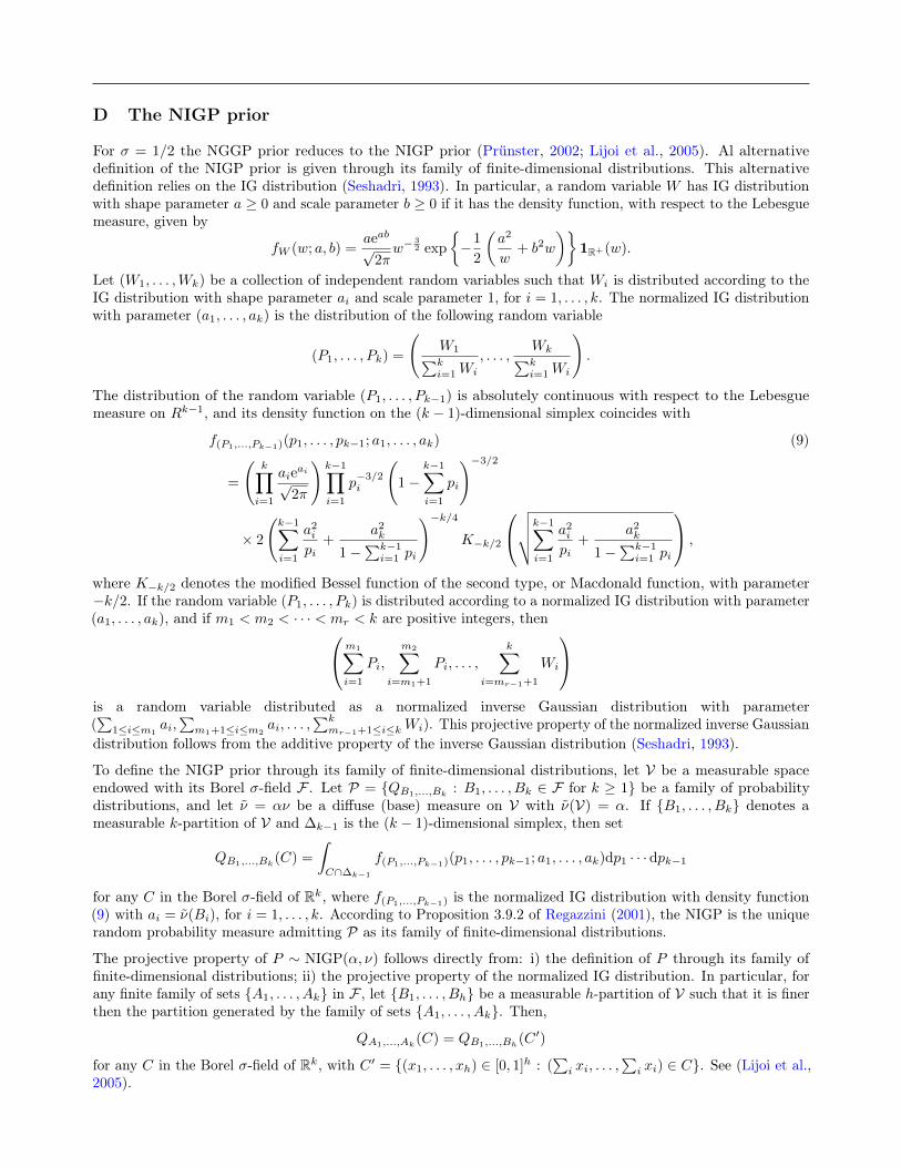
D The NIGP prior

For σ = 1/2 the NGGP prior reduces to the NIGP prior (Prünster, 2002; Lijoi et al., 2005). Al alternativedefinition of the NIGP prior is given through its family of finite-dimensional distributions. This alternativedefinition relies on the IG distribution (Seshadri, 1993). In particular, a random variable W has IG distributionwith shape parameter a ≥ 0 and scale parameter b ≥ 0 if it has the density function, with respect to the Lebesguemeasure, given by

fW (w; a, b) =aeab√

2πw−

32 exp

{−1

2

(a2

w+ b2w

)}1R+(w).

Let (W1, . . . ,Wk) be a collection of independent random variables such that Wi is distributed according to theIG distribution with shape parameter ai and scale parameter 1, for i = 1, . . . , k. The normalized IG distributionwith parameter (a1, . . . , ak) is the distribution of the following random variable

(P1, . . . , Pk) =

(W1∑ki=1Wi

, . . . ,Wk∑ki=1Wi

).

The distribution of the random variable (P1, . . . , Pk−1) is absolutely continuous with respect to the Lebesguemeasure on Rk−1, and its density function on the (k − 1)-dimensional simplex coincides with

f(P1,...,Pk−1)(p1, . . . , pk−1; a1, . . . , ak) (9)

=

(k∏i=1

aieai√2π

)k−1∏i=1

p−3/2i

(1−

k−1∑i=1

pi

)−3/2

× 2

(k−1∑i=1

a2i

pi+

a2k

1−∑k−1i=1 pi

)−k/4K−k/2

√√√√k−1∑

i=1

a2i

pi+

a2k

1−∑k−1i=1 pi

,

where K−k/2 denotes the modified Bessel function of the second type, or Macdonald function, with parameter−k/2. If the random variable (P1, . . . , Pk) is distributed according to a normalized IG distribution with parameter(a1, . . . , ak), and if m1 < m2 < · · · < mr < k are positive integers, thenm1∑

i=1

Pi,

m2∑i=m1+1

Pi, . . . ,

k∑i=mr−1+1

Wi

is a random variable distributed as a normalized inverse Gaussian distribution with parameter(∑

1≤i≤m1ai,∑m1+1≤i≤m2

ai, . . . ,∑kmr−1+1≤i≤kWi). This projective property of the normalized inverse Gaussian

distribution follows from the additive property of the inverse Gaussian distribution (Seshadri, 1993).

To define the NIGP prior through its family of finite-dimensional distributions, let V be a measurable spaceendowed with its Borel σ-field F . Let P = {QB1,...,Bk : B1, . . . , Bk ∈ F for k ≥ 1} be a family of probabilitydistributions, and let ν̃ = αν be a diffuse (base) measure on V with ν̃(V) = α. If {B1, . . . , Bk} denotes ameasurable k-partition of V and ∆k−1 is the (k − 1)-dimensional simplex, then set

QB1,...,Bk(C) =

∫C∩∆k−1

f(P1,...,Pk−1)(p1, . . . , pk−1; a1, . . . , ak)dp1 · · · dpk−1

for any C in the Borel σ-field of Rk, where f(P1,...,Pk−1) is the normalized IG distribution with density function(9) with ai = ν̃(Bi), for i = 1, . . . , k. According to Proposition 3.9.2 of Regazzini (2001), the NIGP is the uniquerandom probability measure admitting P as its family of finite-dimensional distributions.

The projective property of P ∼ NIGP(α, ν) follows directly from: i) the definition of P through its family offinite-dimensional distributions; ii) the projective property of the normalized IG distribution. In particular, forany finite family of sets {A1, . . . , Ak} in F , let {B1, . . . , Bh} be a measurable h-partition of V such that it is finerthen the partition generated by the family of sets {A1, . . . , Ak}. Then,

QA1,...,Ak(C) = QB1,...,Bh(C ′)

for any C in the Borel σ-field of Rk, with C ′ = {(x1, . . . , xh) ∈ [0, 1]h : (∑i xi, . . . ,

∑i xi) ∈ C}. See (Lijoi et al.,

2005).

E Proof of Proposition 2, and proof of Theorem 3

To prove Proposition 2, we start with the following lemma under the assumption that X1:m is a random samplefrom P ∼ NGGP(α, σ, ν). The proof of Proposition 2 then follows by setting σ = 1/2. Let

pfv (`;m,α, σ) =∑

m∈Mk,m

Pr[Xm+1 ∈ v` |Mm = m]Pr[Mm = m], ` = 0, 1, . . . ,m,

where the predictive distributions Pr[Xm+1 ∈ v` |Mm = m] are displayed in Equation 5, and the distributionPr[Mm = m] is displayed in Equation 4. For σ ∈ (0, 1), let fσ denote the density function of the positive σ-stablerandom variable Xσ, i.e. E[exp{−tXσ}] = exp{−tσ} for any t > 0.

Lemma 1. For any m ≥ 1, let X1:m be a random sample from P ∼ NGGP(α, σ, ν). Then, for ` = 0, 1, . . . ,m

pfv (`;m,α, σ)

σ(`−σ)(m` )(1−σ)(`−1)

Γ(1−σ+`)

×∫ +∞

0

∫ 1

01hσ fσ(hp)e−h

(α2−1

σ

) 1σ +α2−1

σ pm−`(1− p)1−σ+`−1dpdh ` < m

α2m(1−σ)(m)

Γ(m+1)

×∫ +∞

0xm

(1+2x)m+1−σ exp{−α2σ−1

σ [(2−1 + x)σ − 2−σ]}

dx ` = m.

(10)

Proof. We start by considering the case ` = 0. The probability pfv (0;m,α, σ) follows by combining Proposition 1with the distribution of Km displayed in (4). Indeed, we can write the following expression

pfv (0;m,α, σ) =∑

m∈Mm,k

Pr[Xm+1 ∈ v0 |Mm = m]Pr[Mm = m] (11)

=∑

m∈Mm,k

Vm+1,k+1

Vm,kPr[Mm = m]

=

m∑k=1

Vm+1,k+1

σkC(m, k;σ). (12)

Then, the expression of pfv (0;m,α, σ) in (10) follows by combining (11) with Vm+1,k+1 displayed in (3), i.e.,

pfv (0;m,α, σ) =(α2σ−1)

Γ(m+ 1)

∫ +∞

0

um

(2−1 + u)m+1−σ exp

{−α2σ−1

σ[(2−1 + u)σ − 2−σ]

}×

m∑k=1

(α2σ−1

σ(2−1 + u)−σ

)kC(m, k;σ)du

[Equation 13 of Favaro et al. (2015)]

=(α2σ−1)

Γ(m+ 1)

∫ +∞

0

um

(2−1 + u)m+1−σ exp

{−α2σ−1

σ[(2−1 + u)σ − 2−σ]

}× exp

{α2σ−1

σ(2−1 + u)−σ

}(α2σ−1

σ(2−1 + u)−σ

)m/σ ∫ +∞

0

xm exp

{−x(

α2σ−1

σ(2−1 + u)−σ

)1/σ}fσ(x)dxdu

[Identity (2−1 + u)−1+σ =1

Γ(1− σ)

∫ +∞

0

y1−σ−1 exp{−y(2−1 + u)

}dy]

=(α2σ−1)1+m/σ

σm/σΓ(m+ 1)

×∫ +∞

0

um(

1

Γ(1− σ)

∫ +∞

0

y1−σ−1 exp{−y(2−1 + u)

}dy

)×

(∫ +∞

0

xm exp

{−x(α2σ−1

σ

) 1σ

u

}exp

{−x(α2−1

σ

) 1σ

+α2−1

σ

}fσ(x)dx

)du

=(α2σ−1)1+m/σ

σm/σΓ(1− σ)

×∫ +∞

0

xmfσ(x) exp

{−x(α2−1

σ

) 1σ

+α2−1

σ

}

×∫ +∞

0

y1−σ−1 exp{−y2−1

}[x

(α2σ−1

σ

) 1σ

+ y

]−n−1

dydx

[Change of variable p =y

x(α2σ−1

σ

) 1σ

+ y

]

=(α2σ−1)1+m/σ

σm/σΓ(1− σ)

×∫ +∞

0

xmfσ(x) exp

{−x(α2−1

σ

) 1σ

+α2−1

σ

}

×∫ 1

0

(α2σ−1

σ

) 1σ

xp

1− p

1−σ−1 (

α2σ−1

σ

) 1σ

x

(1− p)2

× exp

−(α2σ−1

σ

) 1σ

xp

1− p2−1

x(α2σ−1

σ

) 1σ

+

(α2σ−1

σ

) 1σ

xp

1− p

−m−1

dpdx

[Change of variable h = x/(1− p)]

=(α2σ−1)1+m/σ

σm/σΓ(1− σ)

×∫ +∞

0

∫ 1

0

(h(1− p))mfσ(h(1− p)) exp

{−h(1− p)

(α2−1

σ

) 1σ

+α2−1

σ

}

×

((α2σ−1

σ

) 1σ

hp

)1−σ−1(α2σ−1

σ

) 1σ

h

× exp

{−(α2σ−1

σ

) 1σ

hp2−1

}[h(1− p)

(α2σ−1

σ

) 1σ

+

(α2σ−1

σ

) 1σ

hp

]−m−1

dpdh

=(α2σ−1)1+m/σ

σm/σΓ(1− σ)

((α2σ−1

σ

) 1σ

)−σ−m

×∫ +∞

0

∫ 1

0

(h(1− p))nfσ(h(1− p)) exp

{−h(α2−1

σ

) 1σ

+α2−1

σ

}p1−σ−1h−m−σdpdh

=σ

Γ(1− σ)

∫ +∞

0

∫ 1

0

fσ(hp) exp

{−h(α2−1

σ

) 1σ

+α2−1

σ

}h−σpm(1− p)1−σ−1dpdh.

This complete the case ` = 0. Now, we consider ` > 0. The probability pfv(`;m,α, σ) follows by combiningProposition 1 with the distribution of (Km,Nn) displayed in (2). In particular, we can write

pfv (`;m,α, σ) =∑

m∈Mm,k

Pr[Xm+1 ∈ v` |Mm = m]Pr[Mm = m]

=∑

m∈Mm,k

Vm+1,k

Vm,k(`− σ)mlPr[Mm = m]

= (`− σ)

m∑k=1

∑(n1,...,nk)∈Pm,k

1

k!

(m

n1, . . . , nk

)Vm,k

k∏i=1

(1− σ)(ni−1)Vm+1,k

Vm,k

k∑j=1

1nj (`)

= (`− σ)

m∑k=1

Vm+1,k

Vm,k

k∑j=1

Pr[Km = k,Nj = `]

= (`− σ)

m∑k=1

Vm+1,k

Vm,k

k∑j=1

Vm,kk

(n

`

)(1− σ)(`−1)

C(m− `, k − 1;σ)

σk−1

= (`− σ)

(m

`

)(1− σ)(`−1)

m∑k=1

Vm+1,kC(m− `, k − 1;σ)

σk−1. (13)

Then, the expression of pfv (`;m,α, σ) in (10) follows by combining (13) with Vm+1,k displayed in (3), i.e.,

pfv (`;m,α, σ) = (`− σ)

(m

`

)(1− σ)(`−1)

m∑k=1

Vm+1,kC(m− `, k − 1;σ)

σk−1

= (`− σ)

(m

`

)(1− σ)(`−1)

× σ

Γ(m+ 1)

∫ +∞

0

um exp

{−α2σ−1

σ[(2−1 + u)σ − 2−σ]

}(2−1 + u)−m−1du

×m∑k=1

C(m− `, k − 1;σ)

(α2σ−1

σ(2−1 + u)−σ

)k.

If ` = m, then

pfv (m;m,α, σ) = (1− σ)(m)

m∑k=1

Vm+1,kC(0, k − 1;σ)

σk−1

= (1− σ)(m)Vm+1,1

= (1− σ)(m)α2σ−1

Γ(m+ 1)

∫ +∞

0

xm

(2−1 + x)m+1−σ exp

{−α2σ−1

σ[(2−1 + x)σ − 2−σ]

}dx.

If ` < m, then

pfv (`;m,α, σ) = (`− σ)

(m

`

)(1− σ)(`−1)

m∑k=1

Vm+1,kC(m− `, k − 1;σ)

σk−1

= (`− σ)

(m

`

)(1− σ)(`−1)

× α2σ−1

Γ(m+ 1)

∫ +∞

0

um exp

{−α2σ−1

σ[(2−1 + u)σ − 2−σ]

}(2−1 + u)−m−1+σdu

×m−∑̀k=1

C(m− `, k;σ)

(α2σ−1

σ(2−1 + u)−σ

)k[Equation 13 of Favaro et al. (2015)]

= (`− σ)

(m

`

)(1− σ)(`−1)

× α2σ−1

Γ(m+ 1)

∫ +∞

0

um exp

{−α2σ−1

σ[(2−1 + u)σ − 2−σ]

}(2−1 + u)−m−1+σ

× exp

{α2σ−1

σ(2−1 + u)−σ

}(α2σ−1

σ(2−1 + u)−σ

)m−`σ

×∫ +∞

0

xm−` exp

{−x(

α2σ−1

σ(2−1 + u)−σ

) 1σ

}fσ(x)dxdu

[Identity (2−1 + u)−1+σ =1

Γ(1− σ + `)

∫ +∞

0

y1−σ+`−1 exp{−y(2−1 + u)

}dy]

= (`− σ)

(m

`

)(1− σ)(`−1)

× (α2σ−1)(α2σ−1)m−`σ

σm−`σ Γ(m+ 1)

∫ +∞

0

um(

1

Γ(1− σ + `)

∫ +∞

0

y1−σ+`−1 exp{−y(2−1 + u)}dy)

×∫ +∞

0

xm−` exp

{−xu

(α2σ−1

σ

) 1σ

}exp

{−x(α2−1

σ

) 1σ

+α2−1

σ

}fσ(x)dxdu

= (`− σ)

(m

`

)(1− σ)(`−1)

× (α2σ−1)1+m−`σ

σm−`σ Γ(1− σ + `)

∫ +∞

0

xm−`fσ(x) exp

{−x(α2−1

σ

) 1σ

+α2−1

σ

}

×∫ +∞

0

y1−σ+`−1 exp{−y2−1}

[x

(α2σ−1

σ

) 1σ

+ y

]−m−1

dydx

[Change of variable p =y

x(α2σ−1

σ

) 1σ

+ y

]

= (`− σ)

(m

`

)(1− σ)(`−1)

× (α2σ−1)1+m−`σ

σm−`σ Γ(1− σ + `)

∫ +∞

0

xm−`fσ(x) exp

{−x(α2−1

σ

) 1σ

+α2−1

σ

}

×∫ 1

0

(α2σ−1

σ

) 1σ

xp

1− p

1−σ+`−1 (

α2σ−1

σ

) 1σ

x

(1− p)2

× exp

−(α2σ−1

σ

) 1σ

xp

1− p2−1

x(α2σ−1

σ

) 1σ

+

(α2σ−1

σ

) 1σ

xp

1− p

−m−1

dpdx

[Change of variable h = x/(1− p)]

= (`− σ)

(m

`

)(1− σ)(`−1)

× (α2σ−1)1+m−`σ

σm−`σ Γ(1− σ + `)

∫ +∞

0

∫ 1

0

(h(1− p))m−`fσ(h(1− p)) exp

{−h(1− p)

(α2−1

σ

) 1σ

+α2−1

σ

}

×

((α2σ−1

σ

) 1σ

hp

)1−σ+`−1(α2σ−1

σ

) 1σ

h

× exp

{−(α2σ−1

σ

) 1σ

hp2−1

}[h(1− p)

(α2σ−1

σ

) 1σ

+

(α2σ−1

σ

) 1σ

hp

]−m−1

dpdh

= (`− σ)

(m

`

)(1− σ)(`−1)

× (α2σ−1)1+m−`σ

σm−`σ Γ(1− σ + `)

((α2σ−1

σ

) 1σ

)−m−σ+`

×∫ +∞

0

∫ 1

0

(h(1− p))m−`fσ(h(1− p)) exp

{−h(α2−1

σ

) 1σ

+α2−1

σ

}p1−σ+`−1h−m−σ+`dpdh

= (`− σ)

(m

`

)(1− σ)(`−1)

× σ

Γ(1− σ + `)

∫ +∞

0

∫ 1

0

fσ(hp) exp

{−h(α2−1

σ

) 1σ

+α2−1

σ

}h−σpm−`(1− p)1−σ+`−1dpdh.

Remark 2. Here we present an alternative representation of pfv (`;m,α, σ) in (10). It provides a useful tool forimplementing a straightforward Monte Carlo evaluation of pfv (`;m,α, σ). For ` = m,

pfv (m;m,α, σ) =σ(`− σ)

(m`

)(1− σ)(`−1)

Γ(1− σ + `)

×∫ +∞

0

∫ 1

0

1

hσfσ(hp)e−h

(α2−1

σ

) 1σ +α2−1

σ pm−`(1− p)1−σ+`−1dpdh

=1

Γ(m+ 1)

∫ +∞

0

exp

{−h( α

2σ

)1/σ

+α

2σ

}σΓ(m+ 1)

Γ(m+ 1− σ)h−σ

×∫ 1

0

(1− p)m+1−σ−1fσ(hp)dpdh

=(1− σ)(m)

Γ(m+ 1)E

[exp

{−XY

(α2−1

σ

) 1σ

+α2−1

σ

}],

where Y is a Beta random variable with parameter (m− `+σ, 1−σ+ `) and X is a random variable, independentof Y , distributed according to a polynomially tilted σ-stable distribution of order σ, i.e.

Pr[X ∈ dx] =Γ(σ + 1)

Γ(2)x−σfσ(x)dx.

For ` < m,

pfv (`;m,α, σ) =σ(`− σ)

(m`

)(1− σ)(`−1)

Γ(1− σ + `)

×∫ +∞

0

∫ 1

0

1

hσfσ(hp)e−h

(α2−1

σ

) 1σ +α2−1

σ pm−`(1− p)1−σ+`−1dpdh

= (`− σ)

(m

`

)(1− σ)(`−1)

× Γ(m− `+ σ)

Γ(σ)Γ(m+ 1)

×∫ +∞

0

fσ(hp) exp

{−h(α2−1

σ

) 1σ

+α2−1

σ

}Γ(σ + 1)

Γ(2)h−σ

× Γ(m+ 1)

Γ(1− σ + `)Γ(m− `+ σ)

∫ 1

0

pm−`(1− p)1−σ+`−1dpdh

=Γ(m− `+ σ)

Γ(σ)Γ(m+ 1)E

[exp

{−XY

(α2−1

σ

) 1σ

+α2−1

σ

}].

According to this alternative representation, pfv (`;m,α, σ) allows for a Monte Carlo evaluation by sampling froma Beta random variable and from a polynomially tilted σ-stable random variable of order σ. See, e.g., (Devroye,2009).

Proof of Proposition 2. The proof follows by a direct application of Lemma (1) by setting σ = 1/2. First, letrecall that the density function of the (1/2)-stable positive random variable coincides with the IG density function(Seshadri, 1993) with shape parameter a = 2−1/2 and scale parameter b = 0. That is, we write

f1/2(x) =1

2√πw−

32 exp

{− 1

4w

}.

For ` = m,

pfv (m;m,α, σ) =α2m

(12

)(m)

Γ(m+ 1)

×∫ +∞

0

xm

(1 + 2x)m+ 12

exp{−α21/2[(2−1 + x)1/2 − 2−1/2]

}dx.

For ` < m,

pfv (`;m,α, σ) =2−1(`− 2−1)

(m`

) (12

)(`−1)

Γ(2−1 + `)

×∫ +∞

0

∫ 1

0

1√hf1/2(hp)e−hα

2+αpm−`(1− p) 12 +`−1dpdh

= (`− 2−1)

(m

`

)(1− 2−1)(`−1)

× 2−1

2π1/2eα∫ 1

0

∫ +∞

0

h−1−1 exp

{−hα2 −

14p

h

}

× 1

Γ(1− 2−1 + `)pm−`−

12−1(1− p)1− 1

2 +`−1dpdh

[Equation 3.471.9 of Gradshteyn and Ryzhic (2007)]

= (`− 2−1)

(m

`

)(1− 2−1)(`−1)

× eααπ1/2Γ(1− 2−1 + `)

∫ 1

0

K−1

(α

p1/2

)pm−`−1(1− p)1− 1

2 +`−1dp,

where K−1 is the modified Bessel function of the second type, or Macdonald function, with parameter −1.Remark 3. Here we present an alternative representation of pfv (`;m,α, σ) in Proposition 2. It provides a usefultool for implementing a straightforward Monte Carlo evaluation of pfv (`;m,α, σ). For ` = m,

pfv (m;m,α, σ) =α2m

(12

)(m)

Γ(m+ 1)

×∫ +∞

0

xm

(1 + 2x)m+ 12

exp{−α21/2[(2−1 + x)1/2 − 2−1/2]

}dx

=1

Γ(m+ 1)

∫ +∞

0

exp{−hα2 + α

} 2−1Γ(m+ 1)

Γ(m+ 1− 1/2)

1√h

×∫ 1

0

(1− p)m+1− 12−1 1

2√π

(hp)−32 exp

{− 1

4hp

}dpdh

=

(12

)(m)

Γ(m+ 1)E[exp

{−XYα2 + α

}],

where Y is a Beta random variable with parameter (1/2,m+ 1/2) and X is a random variable, independent of Y ,distributed according to a polynomially tilted IG distribution of the order 1/2, that is

Pr[X ∈ dx] =Γ(3/2)

Γ(2)x−

12x−

32

2√π

exp

{− 1

4x

}dx.

For ` < m,

pfv (`;m,α, σ) = (`− 2−1)

(m

`

)(1− 2−1)(`−1)

× eααπ1/2Γ(1− 2−1 + `)

∫ 1

0

K−1

(α

p1/2

)pm−`−1(1− p)1− 1

2 +`−1dp

= (`− 2−1)

(m

`

)(1− 2−1)(`−1)

× Γ(m− `)π1/2Γ(m+ 1− 2−1)

eαα

×∫ 1

0

K−1

(α

p1/2

)Γ(m+ 1− 2−1)

Γ(1− 2−1 + `)Γ(m− `)pm−`−1(1− p)1− 1

2 +`−1dp

= (l − 2−1)

(n

l

)(1− 2−1)(l−1)

× Γ(m− `)π1/2Γ(m+ 1− 2−1)

eααE[K−1

( α

Y 1/2

)],

where Y is a Beta random variable with parameter (m− `, 1/2 + `). According to this alternative representation,pfv (`;m,α, σ) allows for a straightforward Monte Carlo evaluation by sampling from a Beta random variable andfrom a polynomially tilted IG random variable of order 1/2. See, e.g., (Devroye, 2009).

Proof of Theorem 3. Because of the assumption of independence of the hash family, we can factorize the marginallikelihood of (c1, . . . , cN ), i.e. of hash functions h1, . . . , hN , into the product of the marginal likelihoods ofcn = (cn,1, . . . , cn,J), i.e. of each hash function. This, combined with Bayes theorem, leads to

Pr[fv = ` | {Cn,hn(v)}n∈[N ] = {cn,hn(v)}n∈[N ]]

[Bayes theorem and independence of the hash family]

=1

Pr[{Cn,hn(v)}n∈[N ] = {cn,hn(v)}n∈[N ]]Pr[fv = `]

N∏n=1

Pr[Cn,hn(v) = cn,hn(v) | fv = `]

=1

Pr[{Cn,hn(v)}n∈[N ] = {cn,hn(v)}n∈[N ]]Pr[fv = `]

N∏n=1

Pr[Cn,hn(v) = cn,hn(v), fv = `]

Pr[fv = `]

=1

Pr[{Cn,hn(v)}n∈[N ] = {cn,hn(v)}n∈[N ]](Pr[fv = `])1−N

N∏n=1

Pr[Cn,hn(v) = cn,hn(v)]Pr[fv = ` |Cn,hn(v) = cn,hn(v)]

= (Pr[fv = `])1−NN∏n=1

Pr[fv = ` |Cn,hn(v) = cn,hn(v)]

∝N∏n=1

Pr[fv = ` |Cn,hn(v) = cn,hn(v)]

[Proposition 2 and Equation 9]

=∏n∈[N ]

(cn,hn(v)

`)eαJ α

Jπ

∫ 1

0K−1

(α

J√x

)xcn,hn(v)−`−1(1− x)

12 +`−1dx ` = 0, 1, . . . , cn,hn(v) − 1

2cn,hn(v)α( 1

2 )(cn,hn(v))

JΓ(cn,hn(v)+1)

∫ +∞0

xcn,hn(v)

(1+2x)cn,hn(v)+1/2 e

−αJ (√

1+2x−1)dx ` = cn,hn(v),

where K−1(·) is the modified Bessel function of the second type, or Macdonald function, with parameter −1.

F Estimation of α

We start by deriving the marginal likelihood corresponding to the hashed frequencies (c1, . . . , cN ) inducedby the collection of hash functions h1, . . . , hN . In particular, according to the definition of P ∼ NIGP(α, ν)through its family of finite-dimensional distributions, for a single hash function hn the marginal likelihood ofcn = (cn,1, . . . , cn,J) is obtained by integrating the normalized IG distribution with parameter (α/J, . . . , α/J)against the multinomial counts cn. In particular, by means of the normalized IG distribution (9), the marginallikelihood of cn has the following expression

p(cn;α)

=m!∏J

i=1 cn,i!

×∫{(p1,...,pJ−1) : pi∈(0,1) and

∑J−1i=1 pi≤1}

J−1∏i=1

pcn,ii

(1−

J−1∑i=1

pi

)cn,Jf(P1,...,PJ−1)(p1, . . . , pJ−1)dp1 · · · dpJ−1

=m!∏J

i=1 cn,i!

×∫{(p1,...,pJ−1) : pi∈(0,1) and

∑J−1i=1 pi≤1}

(J∏i=1

(α/J)eα/J√2π

)J−1∏i=1

pcn,i−3/2i

(1−

J−1∑i=1

pi

)cn,J−3/2

×∫ +∞

0

z−3J/2+J−1 exp

{− 1

2z

(J−1∑i=1

(α/J)2

pi+

(α/J)2

1−∑J−1i=1 pi

)− z

2

}dzdp1 · · · dpJ−1

[Change of variable pi =xi∑ki=1 xi

, for i = 1, . . . , J − 1, and z =

J∑i=1

xi]

=m!∏J

i=1 cn,i!

×(

(α/J)eα/J√2π

)J ∫(0,+∞)J

J∏i=1

xcn,i−3/2i

(J∑i=1

xi

)−∑Ji=1 cn,i

exp

{−1

2

J∑i=1

(α/J)2

xi− 1

2

J∑i=1

xi

}dx1 · · · dxJ

=m!∏J

i=1 cn,i!

×(

(α/J)eα/J√2π

)J1

Γ(m)

∫(0,+∞)J

J∏i=1

xcn,i−3/2i

(∫ +∞

0

ym−1 exp

{−y

J∑i=1

xi

}dy

)

× exp

{−1

2

J∑i=1

(α/J)2

xi− 1

2

J∑i=1

xi

}dx1 · · · dxJ

=m!∏J

i=1 cn,i!

×(

(α/J)eα/J√2π

)J1

Γ(m)

∫ +∞

0

ym−1

(J∏i=1

∫ +∞

0

xcn,i−3/2i exp

{− (α/J)2

2xi− xi

(y +

1

2

)}dxi

)dy

[Equation 3.471.9 of Gradshteyn and Ryzhic (2007)]

=m!∏J

i=1 cn,i!

×(

(α/J)eα/J√2π

)J1

Γ(m)

∫ +∞

0

ym−1

(J∏i=1

2

((α/J)2

1 + 2y

)cn,i/2−1/4

Kcn,i−1/2

(√c2n,i(1 + 2y)

))dy

=m(αJ

)m+ J2 eα

(π/2)J2

∏Jj=1 cn,j !

∫ +∞

0

ym−1

(1 + 2y)m/2−J/4

(J∏i=1

Kcn,i−1/2

(√(α/J)2

i (1 + 2y)

))dy.

Because of the independence of the hash family, h1, . . . , hN leads to the following marginal likelihood of{cn,j}n∈[N ] j∈[J]

p(c1, . . . , cN ;α) (14)

=∏n∈[N ]

m(αJ

)m+ J2 eα

(π/2)J2

∏Jj=1 cn,j !

∫ +∞

0

xm−1

(1 + 2x)m2 −

J4

J∏j=1

Kcn,j− 12

(√(αJ

)2

(1 + 2x)

) dx.

The marginal likelihood of {cn,j}n∈[N ] j∈[J] in (14) is applied to estimate the mass parameter α. This is theempirical Bayes approach to the estimation of α. In particular, we consider the following problem

arg maxα

∏n∈[N ]

Vn,m,α,J

∫ +∞

0

Fn,m,α,J(y)dy

,

where

Vn,m,α,J =m(αJ

)m+ J2 eα

(π/2)J2

∏Jj=1 cn,j !

and

Fn,m,α,J(y) =ym−1

(1 + 2y)m2 −

J4

J∏j=1

Kcn,j− 12

(√(αJ

)2

(1 + 2y)

)under the constraint that α > 0. To avoid overflow/underflow issues in the above optimization problem, here wework in log-space. That is, we consider the following equivalent optimization problem1

arg maxα

∑n∈[N ]

log(Vn,m,α,J) + log

(∫ +∞

0

Fn,m,α,J(y)dy

)= arg max

α

∑n∈[N ]

vn,m,α,J + log

(∫ +∞

0

exp{fn,m,α,J(y)}dy) ,

with vn,m,α,J = log(Vn,m,α,J) and fn,m,α,J(y) = log(Fn,m,α,J(y)). For the computation of the integral we usedouble exponential quadrature (Takahasi and Mori, 1974), which approximates

∫ +1

−1f(y)dy with

∑mj=1 wjf(yj)

for appropriate weights wj ∈ W and coordinates yj ∈ Y . Integrals of the form∫ baf(y)dy for −∞ ≤ a ≤ b ≤ +∞

are handled via change of variable formulas. To avoid underflow/overflow issues it is necessary to apply the"log-sum-exp" trick to the above integral. That is,

log

(∫ +∞

0

exp{fn,m,α,J(y)}dy)

= f∗ + log

(∫ +∞

0

exp{fn,m,α,J(y)− f∗}dy)

and

f∗ = arg maxy∈Y

{fn,m,α,J(y)} .

The computation of log(Kcn,j− 12(x)) is performed via the following finite-sum representation of Kcn,j− 1

2(x), which

holds for Kv(x) when v is an half-integer. Recall that Kv(x) is symmetric in v. In particular,

Kcn,i−1/2

(√(α/J)(1 + 2y)

)=

√π

2

exp{−((α/J)(1 + 2y))1/2

}((α/J)(1 + 2y))1/4

cn,i−1∑j=0

(j + cn,i − 1)!

j! (cn,i − j − 1)!(2((α/J)(1 + 2y))1/2)−j .

In order to increase efficiency in the our optimization, we cache the log-factorials and, anew for each α and y thevalues of log(Kcn,j− 1

2(√

(α/J)2(1 + 2y))) across j. In particular, as the dependency on j goes through cn,j onlywe can exploit the fact that many duplicates exists, i.e. the complexity scales in the number of unique cn,j . Allcode is implemented in LuaJIT2 by using the scilua3 library.

1the computation of log-factorials is done via the specialized implementation of the log-gamma function2https://luajit.org3https://scilua.org

G Additional experiments

We present additional experiments on the application of the CMS-NIGP on synthetic and real data. First, werecall the synthetic and real data to which the CMS-NIGP is applied. As regards synthetic data, we considerdatasets of m = 500.000 tokens from a Zipf’s distributions with parameter s = 1.3, 1.6, 1.9, 2, 2, 2.5. As regardsreal data, we consider: i) the 20 Newsgroups dataset, which consists of m = 2.765.300 tokens with k = 53.975distinct tokens; ii) the Enron dataset, which consists of m = 6412175 tokens with k = 28102 distinct tokens.Tables 1, 2, 3 and 4 report the MAE (mean absolute error) between true frequencies and their correspondingestimates via: i) the CMS-NIGP estimate f̂ (NIGP)

v ; ii) the CMS estimate f̂ (CMS)v ; iii) the CMS-DP estimatef̂ (DP)

v ,the CMM estimate f̂ (CMM)

v .

ReferencesBacallado, S., Battiston, M., Favaro, S., and Trippa, L. (2017). Sufficientness postulates for gibbs-type priors andhierarchical generalizations. Statistical Science, 32:487–500.

Cai, D., Mitzenmacher, M., and Adams, R. P. (2018). A Bayesian nonparametric view on count-min sketch. InAdvances in Neural Information Processing Systems.

Charalambides, C. A. (2005). Combinatorial methods in discrete distributions, volume 600. John Wiley & Sons.

Cormode, G. and Muthukrishnan, S. (2005a). An improved data stream summary: the count-min sketch and itsapplications. Journal of Algorithms, 55:58–75.

Cormode, G. and Muthukrishnan, S. (2005b). Summarizing and mining skewed data streams. In Proceedings ofthe 2005 SIAM International Conference on Data Mining.

De Blasi, P., Favaro, S., Lijoi, A., Mena, R. H., Prünster, I., and Ruggiero, M. (2013). Are Gibbs-type priorsthe most natural generalization of the Dirichlet process? IEEE transactions on pattern analysis and machineintelligence, 37:212–229.

Devroye, L. (2009). Random variate generation for exponentially and polynomially tilted stable distributions.ACM Transactions on Modeling and Computer Simulation, 19.

Ewens, W. (1972). The sampling theory of selectively neutral alleles. Theoretical Population Biology, 3:87–112.

Favaro, S., Nipoti, B., and Teh, Y. (2015). Random variate generation for laguerre-type exponentially tiltedalpha-stable distributions. Electronic Journal of Statistics, 9:1230–1242.

Gradshteyn, I. and Ryzhic, I. (2007). Table of integrals, series and products. Academic Press.

James, L. F. (2002). Poisson process partition calculus with applications to exchangeable models and Bayesiannonparametrics. arXiv preprint arXiv:math/0205093.

Kingman, J. (1993). Poisson processes. Wiley Online Library.

Lijoi, A., Mena, R. H., and Prünster, I. (2005). Hierarchical mixture modeling with normalized inverse-Gaussianpriors. Journal of the American Statistical Association, 100:1278–1291.

Lijoi, A., Mena, R. H., and Prünster, I. (2007). Controlling the reinforcement in Bayesian non-parametric mixturemodels. Journal of the Royal Statistical Society Series B, 69:715–740.

Lijoi, A. and Prünster, I. (2010). Models beyond the Dirichlet process. In Bayesian Nonparametrics, Hjort, N.L.,Holmes, C.C. Müller, P. and Walker, S.G. Eds. Cambridge University Press.

Pitman, J. (2003). Poisson-Kingman partitions. In Science and Statistics: A Festschrift for Terry Speed. Instituteof Mathematical Statistics.

Pitman, J. (2006). Combinatorial stochastic processes. Lecture Notes in Mathematics. Springer-Verlag.

Prünster, I. (2002). Random probability measures derived from increasing additive processes and their applicationto Bayesian statistics. Ph.D Thesis, University of Pavia.

Regazzini, E. (2001). Foundations of Bayesian statistics and some theory of Bayesian nonparametric methods.Lecture Notes, Stanford University.

Regazzini, E., Lijoi, A., and Prünster, I. (2003). Distributional results for means of normalized random measureswith independent increments. The Annals of Statistics, 31:560–585.

Seshadri, V. (1993). The inverse Gaussian distribution. Oxford University Press.

Takahasi, H. and Mori, M. (1974). Double exponential formulas for numerical integration. Publications of theResearch Institute for Mathematical Sciences, 9(3):721–741.

Table

1:Synthetic

data:M

AE

forf̂(N

IGP)

v,f̂(C

MM

)v

andf̂(C

MS)

v,case

J=

320,N

=2

Z1.3

Z1.6

Z1.9

Z2.2

Z2.5

Bins

vf̂

(CM

S)

vf̂

(CM

M)

vf̂

(NIG

P)

vf̂

(CM

S)

vf̂

(CM

M)

vf̂

(NIG

P)

vf̂

(CM

S)

vf̂

(CM

M)

vf̂

(NIG

P)

vf̂

(CM

S)

vf̂

(CM

M)

vf̂

(NIG

P)

vf̂

(CM

S)

vf̂

(CM

M)

vf̂

(NIG

P)

v

(0,1]1,061.3

161.72231.31

629.4062.19

134.75308.11

81.1065.71

51.651.04

12.9132.65

1.027.16

(1,2]1,197.9

169.74287.43

514.31102.42

119.22154.20

2.0037.03

289.502.04

61.8748.15

2.019.88

(2,4]1,108.3

116.37262.18

474.8252.10

95.782,419.51

2215.85353.73

134.053.40

26.9054.34

10.5010.09

(4,8]1,275.9

378.04302.89

786.73214.46

175.10460.13

258.9083.30

118.406.44

21.5869.85

6.0314.28

(8,16]1,236.1

230.32257.08

719.84232.24

136.66380.05

139.5066.44

413.13129.03

77.3980.80

13.1020.15

(16,32]1,256.8

221.98248.41

831.7079.73

190.05288.59

23.9041.99

503.60364.30

90.299.86

22.3915.36

(32,64]1,312.8

235.87284.12

783.90184.99

139.52415.58

54.8267.30

217.8182.92

48.0010.22

30.9028.90

(64,128]1,721.7

766.29312.59

950.31304.36

125.071,875.50

1762.20353.10

64.0197.40

65.9113.75

96.9866.18

(128,256]1,107.7

334.5797.91

1,727.191488.38

273.50202.09

163.61110.32

46.80156.71

130.9417.51

181.38125.75

Tab

le2:

Synt

heti

cda

ta:

MA

Efo

rf̂(N

IGP)

v,f̂(C

MM

)v

andf̂(C

MS)

v,ca

seJ

=160,N

=4

Z1.3

Z1.6

Z1.9

Z2.2

Z2.5

Binsv

f̂(C

MS)

vf̂

(CM

M)

vf̂

(NIG

P)

vf̂

(CM

S)

vf̂

(CM

M)

vf̂

(NIG

P)

vf̂

(CM

S)

vf̂

(CM

M)

vf̂

(NIG

P)

vf̂

(CM

S)

vf̂

(CM

M)

vf̂

(NIG

P)

vf̂

(CM

S)

vf̂

(CM

M)

vf̂

(NIG

P)

v

(0,1]

212.1

590.48

0.94

262.00

146.11

0.25

424.8

130.90

0.18

154.79

47.10

0.32

56.7

1.01

0.38

(1,2]

339.8

359.57

0.56

332.75

63.21

0.70

552.0

65.00

0.82

182.72

2.01

1.24

48.2

2.03

1.45

(2,4]

270.9

69.42

1.33

277.80

301.89

2.47

487.3

163.55

2.53

184.70

97.15

2.66

57.8

14.35

2.74

(4,8]

234.6

339.95

4.69

375.74

579.94

4.67

545.2

243.08

5.28

252.53

62.70

5.96

51.1

8.30

5.42

(8,16]

213.3

313.37

10.57

165.73

152.53

10.68

493.2

196.20

10.86

247.33

29.70

10.28

24.1

14.11

11.75

(16,32]

283.0

23.30

20.72

217.20

22.94

19.21

535.5

154.30

22.08

295.90

190.92

21.57

25.0

23.20

23.37

(32,64]

305.7

133.09

42.66

284.61

209.13

43.14

637.8

150.05

42.64

120.62

71.86

44.49

31.7

40.40

44.03

(64,128]

244.5

102.43

92.26

120.21

118.42

94.43

425.1

198.60

95.19

180.30

113.75

95.10

29.2

94.73

93.34

(128,256]

237.4

294.43

170.09

141.30

573.12

173.87

525.9

267.15

185.83

129.70

176.50

180.41

32.1

119.19

179.51

Table 3: Real data (J = 12000 and N = 2): MAE for f̂(NIGP)v , f̂(DP)

v and f̂(CMS)v

20 Newsgroups Enron

Bins for true v f̂ (CMS)v f̂ (DP)

v f̂ (NIGP)v f̂ (CMS)

v f̂ (DP)v f̂ (NIGP)

v

(0,1] 46.4 46.39 11.34 12.2 12.20 3.00(1,2] 16.6 16.60 3.53 13.8 13.80 3.06(2,4] 38.4 38.40 7.71 61.5 61.49 12.55(4,8] 59.4 59.39 10.40 88.4 88.39 17.36(8,16] 54.3 54.29 11.34 23.4 23.40 4.58(16,32] 17.8 17.80 9.85 55.1 55.09 11.58(32,64] 40.8 40.79 25.65 128.5 128.48 39.46(64,128] 26.0 25.99 57.95 131.1 131.08 54.42(128,256] 13.6 13.59 126.07 50.7 50.68 119.04

Table 4: Real data (J = 8000 and N = 4): MAE for f̂(NIGP)v , f̂(DP)

v and f̂(CMS)v

20 Newsgroups Enron

Bins for true v f̂ (CMS)v f̂ (DP)

v f̂ (NIGP)v f̂ (CMS)

v f̂ (DP)v f̂ (NIGP)

v

(0,1] 53.4 53.39 0.39 71.0 70.98 0.41(1,2] 30.5 30.49 1.40 47.4 47.38 1.47(2,4] 32.5 32.49 2.70 52.5 52.49 3.25(4,8] 38.7 38.69 5.97 53.1 53.08 6.17(8,16] 25.3 25.29 11.97 57.0 56.98 11.28(16,32] 25.0 24.99 21.25 90.0 89.98 19.82(32,64] 39.7 39.69 42.81 108.4 108.37 47.07(64,128] 22.1 22.09 91.06 55.7 55.67 87.32(128,256] 25.8 25.79 205.58 80.8 80.76 178.23