A test strategy for spurious spatial regression, spatial nonstationarity, and spatial cointegration

1

A Test Strategy for Spurious Spatial Regression,

Spatial Nonstationarity,

and Spatial Cointegration.

Jørgen Lauridsen1

Reinhold K osfeld 2

1 Corresponding author: Associate Professor, Department of Statistics and Demography,

University of Southern Denmark, Campusvej 55, DK-5230 Odense M, Denmark

Fax +45 6595 7766 E-mail [email protected]

Homepage http://www.ou.dk/tvf/statdem/people/lauridsen.html .

2 Professor, Department of Economics, University of Kassel, D-34109 Kassel, Germany.

E-mail [email protected]

Homepage http://www.wirtschaft.uni-kassel.de/Kosfeld/

2

ABSTRACT

A test strategy consisting of a twofold application of a Lagrange Multiplier test is suggested as

a device to reveal spatial nonstationarity and spurious spat ial regeression. It is further illustrated

how the test strategy can be used as a diagnostic for presence of a spatial cointegrating

relationship between two variables. Using Monte Carlo simulations it is shown that the small

sample behaviour of the test strategy is as desired in these cases.

JEL Classifications: C21; C40; C51; J60.

Keywords: Spat ial nonstationarity, spat ial cointegration, spurious regression.

3

1. INTRODUCTION

Spatial regression has been discussed widely in books dedicated to developments in spatial

econometrics, notably by Anselin (1988a), and Anselin and Florax (1995). The consequenses for

estimation and inference in the presence of stable spatial processes have been extensively

investigated (Haining 1990; Anselin 1988a; Bivand 1980; Richardson 1990; Richardson and

Hèmon 1981; Clifford and Richardson 1985; Clifford, Richardson and Hèmon 1989). A recent

study (Fingleton 1999) takes the first steps into analyses of implications of spatial unit roots,

spatial cointegration and spatial error correction models. A follow-up to this study is found in Mur

(2002), where the concept of spurious spat ial regression is established in a framework of spatial

trend (non)stationarity. In Lauridsen (2002) estimation of spatial error-correction models using

an IV approach is investigated.

The present paper refines the suggestions of Fingleton (1999). Specifically, Fingleton suggests that

“very high” values of Morans I test for spatial residual autocorrelation indicate spatial

nonstationarity and spurious regression. It is, however, left as an open question how to distinguish

between stationary positive autocorrelation and nonstationarity. The present investigation shows

that a twofold application of the LM test for residual autocorrelation can provide a better founded

basis to separate these two cases. It is further shown that the same procedure works as a

diagnostic for spurious regression. Next, it is suggested that the test procedure works well as a

test for spatial cointegration, using a specific two-variable data generating process. In all cases,

the small-sample properties of the suggested procedures are derived using Monte Carlo

simulation. It is concluded that the procedure works well in all cases, even for fairly small sample

sizes. Finally, the practical applicability of the suggested approach is shortly illustrated using two

4

cases from recent empirical research.

2. MODELS WITH SPATIAL DYNAMICS

2.1. The regressive, spatial autoregressive model.

The first order spatial autoregressive model [SAR(1) model] was initially studied by Whitt le

(1954) and has been used extensively in works by Ord (1975); Cliff and Ord (1981); Ripley

(1981); Upton and Fingleton (1985); Anselin (1988a); Griffith (1992); Haining (1990); Lauridsen

(2002). The regressive, first order spatial autoregressive model [SARX(1) model] is defined by

(2.1) y = DWy + X$ + , , ,-N(0 , F2I) ,

in which y is an n×1 vector, X an n×K matrix of exogenous variables, D the autoregressive

parameter, I the n×n identity matrix, , an n×1 vector of white noises distributed with variances

F2, and W an n×n proximity matrix defined by Wij = 1 if observation j is assumed to impact

observation i, and Wij = 0 otherwise (Footnote 1). W may be noncircular, which is the case for the

time series variant where Wij = 1 if j = i-1, for i = 2,3,..,n. For the general spatial case, W is

generally circular. For example, if the sample consists of a cross-section of n regions, W is usually

defined by Wij = Wji = 1 if region i and j are neighbours. As proved by Anselin (1988a), circularity

of W renders OLS estimation of the parameters inconsistent. This is in contrast to the time series

case (and any other non-circular cases) where OLS provides consistent (although inefficient)

estimation.

5

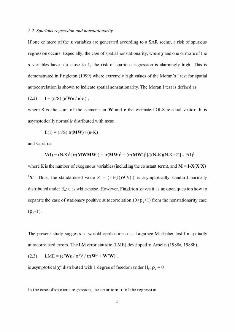
2.2. Spurious regression and nonstationarity.

If one or more of the x variables are generated according to a SAR sceme, a risk of spurious

regression occurs. Especially, the case of spatial nonstationarity, where y and one or more of the

x variables have a D close to 1, the risk of spurious regression is alarmingly high. This is

demonstrated in Fingleton (1999) where extremely high values of the Moran’s I test for spatial

autocorrelation is shown to indicate spatial nonstationarity. The Moran I test is defined as

(2.2) I = (n/S) (e’We / e’e ) ,

where S is the sum of the elements in W and e the estimated OLS residual vector. It is

asymptotically normally distributed with mean

E(I) = (n/S) tr(MW) / (n-K)

and variance

V(I) = (N/S)2 [tr(MWMW’) + tr(MW)2 + (tr(MW))2]/[(N-K)(N-K+2)] - E(I)2

where K is the number of exogenous variables (including the constant term), and M = I-X(X’X)-

1X’. Thus, the standardised value Z = (I-E(I))//V(I) is asymptotically standard normally

distributed under H0: , is white-noise. However, Fingleton leaves it as an open question how to

separate the case of stationary positive autocorrelation (0<De<1) from the nonstationarity case

(De=1).

The present study suggests a twofold application of a Lagrange Multiplier test for spatially

autocorrelated errors. The LM error statistic (LME) developed in Anselin (1988a, 1988b),

(2.3) LME = (e’We / F2)2 / tr(W2 + W’W) .

is asymptotical P2 distributed with 1 degree of freedom under H0: De = 0

In the case of spurious regression, the error term , of the regression

6

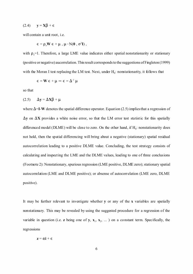
(2.4) y = X$ + ,

will contain a unit root, i.e.

, = DeW , + : , :-N(0 , F2I) ,

with De=1. Therefore, a large LME value indicates either spatial nonstationarity or stationary

(positive or negative) aucorrelation. This result corresponds to the suggestions of Fingleton (1999)

with the Moran I test replacing the LM test. Next, under H0: nonstationarity, it follows that

, = W , + : ] , = )-1 :

so that

(2.5) )y = )X$ + :

where )=I-W denotes the spatial difference operator. Equat ion (2.5) implies that a regression of

)y on )X provides a white noise error, so that the LM error test sta tist ic for this spatially

differenced model (DLME) will be close to zero. On the other hand, if H0: nonstationarity does

not hold, then the spatial differencing will bring about a negative (stationary) spatial residual

autocorrelation leading to a positive DLME value. Concluding, the test strategy consists of

calculating and inspect ing the LME and the DLME values, leading to one of three conclusions

(Footnote 2): Nonstationary, spurious regression (LME positive, DLME zero); stationary spatial

autocorrelation (LME and DLME positive); or absense of autocorrelation (LME zero, DLME

positive).

It may be further relevant to investigate whether y or any of the x variables are spatially

nonstationary. This may be revealed by using the suggested procedure for a regression of the

variable in question (i.e. z being one of y, x1, x2, ... ) on a constant term. Specifically, the

regressions

z = "i + ,

7

and

)z = ")i + ,

readily provide the LME and DLME test statistics, which lead to one of three conclusions: z is

spatially nonstat ionary (LME positive, DLME zero); z represents a stationary SAR scheme (LME

positive, DLME positive); or z is free of any spatial pattern (LME zero, DLME positive).

A further advantage of the LM test strategy is that it is quite flexible. Thus, it is possible to control

for omitted model features insofar that these can be incorporated as part of the likelihood function.

For example, it is straightforward to account for omitted heterogeneity and an omitted

autoregression in the dependent variable, along the lines suggested in Anselin (1988b).

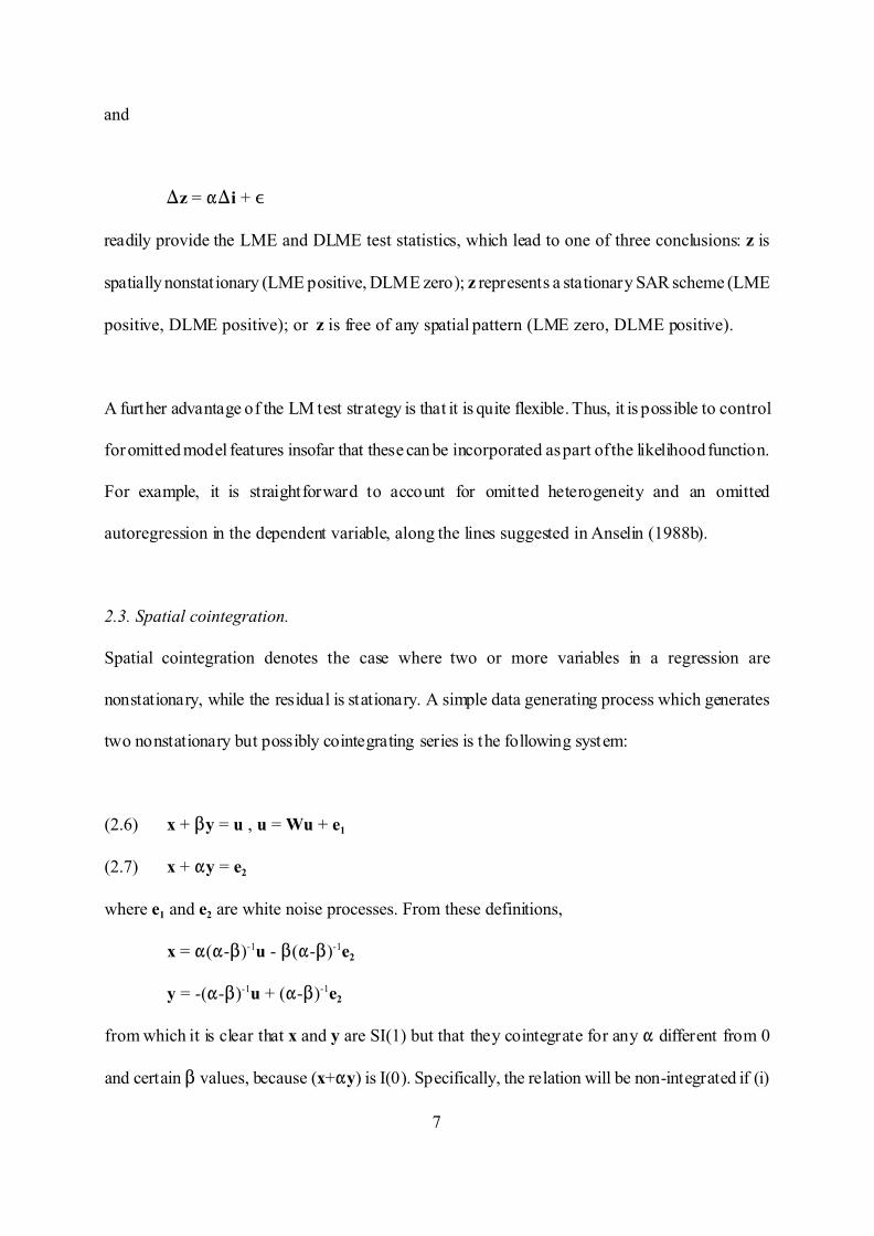
2.3. Spatial cointegration.

Spatial cointegration denotes the case where two or more variables in a regression are

nonstationary, while the residual is stationary. A simple data generating process which generates

two nonstationary but possibly cointegrating series is the following system:

(2.6) x + $y = u , u = Wu + e1

(2.7) x + "y = e2

where e1 and e2 are white noise processes. From these definitions,

x = "("-$)-1u - $("-$)-1e2

y = -("-$)-1u + ("-$)-1e2

from which it is clear that x and y are SI(1) but that they cointegrate for any " different from 0

and certain $ values, because (x+"y) is I(0). Specifically, the relation will be non-integrated if (i)

8

"=0 or (ii) ">0 and $>".

We suggest that the above LM strategy may apply to this situation. Specifically, a regression of

y on X represents a cointegrat ing relation (if LME is zero and DLME is negative) or a non-

integrating relation (if LME is positive and DLME is zero). The limiting case of “near integration”

(">0, $>") will be also be revealed (if LME and DLME are positive).

3. Monte Carlo simulation studies: Designs and results.

In the following section, the small-sample properties of the above suggested test strategies will

be investigated using Monte Carlo simulation studies. The chosen Monte Carlo designs are

outlined together with the results.

3.1. Spurious regression.

To investigate the finite sample properties of the suggested LME test strategy for spurious

regression, the following Monte Carlo design were investigated. To reflect reality, we assume a

multiple regression where some of the explanatory variables are stationary and some nonstatio-

nary. Specifically, we employ four explanatory variables, of which two are nonstationary and two

are white noise processes. The specific design were as follows:

For specific sample size n: Perform 10,000 iterations:

Generate e0, e1, e2, e3, e4 as independent N(0,1) series.

Let e = (I-DeW)-1e0.

Let xi = (I-DxW)-1ei, i=1,2.

Let xi = ei , i=3,4.

9

Let y = i + x1 + x2 + x3 + x4 + e.

Regress y on X = [i x1 x2 x3 x4 ] and )y on )X. Report LME and DLME.

Report the percentage of cases out of 10,000 where LME, respective DLME exceeds

the 5 per cent critical value of P2(1) = 3.84.

To investigate the impact of contiguity matrix type, we used rook and queen type contiguity

matrices based on an r×r board (so that n = r2) with r assumed to take the values 5, 10, 15, and

20. In this as well as the following simulations, we followed the usual convention and employed

a row-standardized W matrix, i.e. Wij were replaced by Wij /Ej=1..nWij. Further, the behaviour of

the strategy under H0 : nonstationarity as well as H1 : stationarity (including the case of near

nonstationarity) were investigated by assuming De to take the values 0, 0.5, 0.9, 0.99 and 1. For

each of these, Dx is assumed to take the values 0, 0.5 and 1.

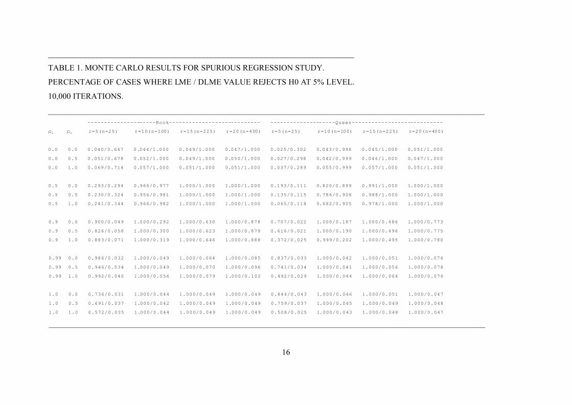
The results are provided in Table 1.

(table 1 around here)

Table 1 shows that the procedure performs well, and that the performance of the procedure is

acceptable, even for fairly small sample sizes. That t he case of near nonstationarity causes

problems in identifying the “true” data generating process is well-known from time series analysis.

However, contrary to time series analysis spatial dependence of moderate size (i.e. r values of

about 0.5) in economic systems seems to be much more reasonable than the case of near-

nonstationarity (see e.g. Rey and Montouri, 1999; Kosfeld, Eckey and Dreger, 2002). Further, the

performance of the procedure seems to be unaffected by the type of contiguity matrix, as the rook

and the queen cases provide similar results.

10

3.2. Test for nonstationarity.

To investigate the finite sample properties of the suggested LME test strategy for nonstationaity

of a single variable, the following Monte Carlo design was investigated:


Generate e as independent N(0,1) series.

Let y = (I-DW)-1e.

Regress y on X = i and )y on )X. Report LME and DLME.



Again, we used the rook and queen type contiguity matrices based on an r×r board with r assumed

to take the values 5, 10, 15, and 20. Further, the behaviour of the strategy under H0 : nonstatio-

narity as well as H1 : stationarity (including the case of near nonstationarity) were investigated by

varying D between the values 0, 0.5, 0.9, 0.99 and 1.



As Table 2 shows that the procedure performs well even for fairly small sample sizes. This holds

true under the assumption of nonstationarity as well as different stationarity cases. The case of

near nonstationarity is again included for comparative purposes. Note that performance is

independent of contiguity matrix type.

11

3.3. Test for cointegration.

To investigate the finite sample properties of the suggested LME test strategy for cointegration

using the suggested example, the following Monte Carlo design was investigated:


Generate e1, e2 as independent N(0,1) series.

Let u = (I-W)-1e1.

Let x = "("-$)-1u - $("-$)-1e2 and y = -("-$)-1u + ("-$)-1e2.

Regress y on X = [i x] and )y on )X. Report LME and DLME.



To investigate the impact of contiguity matrix type, we again used the rook and queen type

contiguity matrices based on an r×r board with r assumed to take the values 5, 10, 15, and 20.

Further, the behaviour of the strategy under H0 : nonstationarity as well as H1 : stationarity

(including the case of near nonstationarity) were investigated by varying " and $ between the

values shown in Table 3.



Table 3 shows that the procedure performs well, especially for fairly large n, and that the

performance of the procedure is acceptable, even for fairly small sample sizes. Especially, in the

case of cointegrat ion ("=1) and non-integrat ion ("=0), the procedure works excellently, while the

12

greyzone case of near-integration (0<"<1, $>") is charachterized by inconclusive test sizes.These

conclusions hold for both types of contiguity matrices, with a single exception for the cases where

" and $ are close to each other. In such cases, the rejection percentages are much higher for the

queen than for the rook case.

4. AN EMPIRICAL ILLUSTRATION

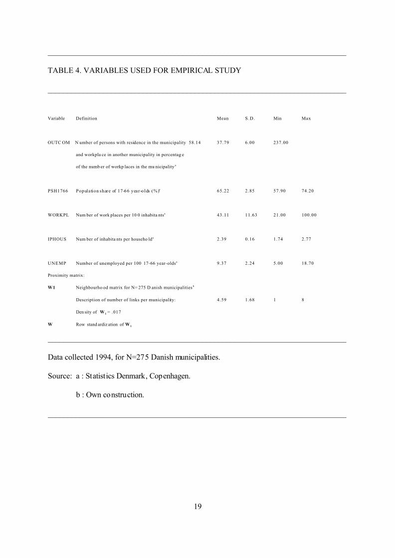
To illustrate the above concepts, we provide an empirical example invest igated in Lauridsen and

Nahrstedt (1999) and Lauridsen (2002). The model is concerned with determination of a

regression model for outcommuting ratios as a function of unemployment, participation rate,

density of working places and average household size. Data were from a 1994 census for 275

Danish municipalities. See Table 4 for a description of the data.


Table 5 presents the estimated model. In Lauridsen (2002) it was left as an open question whether

the unexpected negative sign for the UNEMP coefficient was caused by spuriosity due to spatial

nonstationarity. The Lagrange Multiplier tests for spatial nonstationarity, provided in Table 5,

points to stationarity of the residuals as well as of the single variables. It is concluded that the

single variables as well as the ent ire regression are stationary. Thus, the negative sign for

unemployment is rather due to structural propert ies than to spat ial nonstationarity.


13

5. CONCLUSIONS

Until now, it has not been well established how to separate the case of spatial nonstationarity from

the case of stationary positive autocorrelation. As a consequence, reliable diagnostics for spurious

spatial regression and for the existence of spatial cointegrat ing relations have not been available.

The present study aims to contribute to close these gaps by proposing a st rategy for detecting

spatial nonstationarity. It is shown that the strategy of a twofold application of a Lagrange

Multiplier test provides adequate diagnostics for both spurious spatial regression and the presence

of spatial cointegrating relations. By means of Monte Carlo simulat ions it is demonstrated that the

finite sample properties of the suggested methodology are as desired.

FOOTNOTES

1. A further generalization, which is not in focus of the present study, is to allow the non-zero

units to be different from 1. In this way, it is possible to apply weights to the strength of the

impact from observation i onto observation j.

2. The test result is termed to be “positive” if the LM test statistic differs significantly from zero

and “zero” otherwise.

14

REFERENCES

Anselin L (1988a) Spatial Econometrics: Methods and Models. Kluwer.

Anselin L (1988b) Lagrange Multiplier Tests Diagnostics for Spatial Dependence and Spatial

Heterogeneity. Geographical Analysis, 20, 1-17.

Anselin L, Florax RJGM (eds.)(1995) New Directions in Spatial Econometrics. Springer-

Verlag.

Bivand R (1980) A Monte-Carlo Study of Correlation Coefficient Estimation with Spatially

Autocorrelated Observations. Quaestiones Geographicae, 6, 5-10.

Cliff AD, Ord JK (1981) Spatial Processes: Models and Applications. Pion.

Clifford P, Richardson S (1985) Test ing the Association between Two Spatial Processes.

Statistics and Decisions, Supplement no. 2, 155-60.

Clifford P, Richardson S, Hémon D (1989) Assessing the Significance of the Correlation

between Two Spatial Processes. Biometrics, 45, 123-34.

Fingleton B (1999) Spurious Spatial Regression: Some Monte Carlo Results with a Spatial

Unit Root and Spatial Cointegration. Journal of Regional Science, 39, 1-19.

Greene WH (2000) Econometric Analysis. Prent ice-Hall.

Griffith DA (1992) Simplifying the Normalizing Factor in Spatial Autoregressions for Irregular

Lattices. Papers in Regional Science, 71 71-86.

Haining RP(1990) Spatial Data Analysis in the Social and Environmental Sciences. Cambrid-

ge University Press.

Kosfeld R, Eckey H-F, Dreger C (2002) Regional Convergence in Unified Germany: A Spatial

Econometric Perspective. Discussion Papers in Economics, 39/02, Department of Economics,

University of Kassel, Germany.

Lauridsen J (2002) Spatial autoregressively distributed lag models: equivalent forms, estima-

15

tion, and an illustrative commuting model. Discussion paper, Department of Statistics and

Demography, University of Southern Denmark (Conditionally accepted, Journal of Regional

Science).

Lauridsen J, Nahrstedt B (1999) Spatial Patterns in Intermunicipal Danish Commuting. In G.

Crampton (ed.): Regional Unemployment, Job Matching, and Migration, 49-62, Pion Limited.

Mur J (2002) On the specification of spatial econometric models. Discussion paper, Departa-

mento de Análisis Económico, University of Zaragoza.

Ord JK (1975) Estimation Methods for Models of Spatial Interaction. Journal of the American

Statistical Association, 70, 120-6.

Rey S, Montouri B (1999) US Regional Income Convergence: A Spatial Econometric

Perspective. Regional Studies, 33, 146-156.

Richardson S (1990) Some Remarks on the Testing of Association between Spatial Processes.

In Griffith DA (ed.) Spatial Statistics: Past, Present and Future. Image.

Richardson S, Hémon D (1981) On the Variance of the Sample Correlation between Two

Independent Lattice Processes. Journal of Applied Probability, 18, 943-8.

Ripley BD (1981) Spatial Statistics. Wiley.

Upton GJG, Fingleton B (1985) Spatial Data Analysis by Example, vol. 1. Wiley.

Whittle P (1954) On Stationary Processes in the Plane. Biometrika, 41, 434-49.

16

___________________________________________________________________________

TABLE 1. MONTE CARLO RESULTS FOR SPURIOUS REGRESSION STUDY.

PERCENTAGE OF CASES WHERE LME / DLME VALUE REJECTS H0 AT 5% LEVEL.

10,000 ITERATIONS.

___________________________________________________________________________________________________________

---------------------Rook---------------------------- --------------------Queen----------------------------

De Dx r=5(n=25) r=10(n=100) r=15(n=225) r=20(n=400) r=5(n=25) r=10(n=100) r=15(n=225) r=20(n=400)

0.0 0.0 0.040/0.647 0.044/1.000 0.049/1.000 0.047/1.000 0.025/0.302 0.043/0.998 0.045/1.000 0.051/1.000

0.0 0.5 0.051/0.678 0.052/1.000 0.049/1.000 0.050/1.000 0.027/0.298 0.042/0.999 0.046/1.000 0.047/1.000

0.0 1.0 0.069/0.714 0.057/1.000 0.051/1.000 0.051/1.000 0.037/0.289 0.055/0.999 0.057/1.000 0.051/1.000

0.5 0.0 0.293/0.294 0.966/0.977 1.000/1.000 1.000/1.000 0.193/0.111 0.820/0.899 0.991/1.000 1.000/1.000

0.5 0.5 0.230/0.324 0.956/0.981 1.000/1.000 1.000/1.000 0.135/0.115 0.786/0.908 0.988/1.000 1.000/1.000

0.5 1.0 0.241/0.344 0.966/0.982 1.000/1.000 1.000/1.000 0.065/0.118 0.682/0.905 0.978/1.000 1.000/1.000

0.9 0.0 0.900/0.049 1.000/0.292 1.000/0.630 1.000/0.878 0.707/0.022 1.000/0.187 1.000/0.486 1.000/0.773

0.9 0.5 0.826/0.058 1.000/0.300 1.000/0.623 1.000/0.879 0.616/0.021 1.000/0.190 1.000/0.496 1.000/0.775

0.9 1.0 0.883/0.071 1.000/0.319 1.000/0.646 1.000/0.888 0.372/0.025 0.999/0.202 1.000/0.495 1.000/0.780

0.99 0.0 0.986/0.032 1.000/0.049 1.000/0.064 1.000/0.085 0.837/0.033 1.000/0.042 1.000/0.051 1.000/0.074

0.99 0.5 0.946/0.034 1.000/0.049 1.000/0.070 1.000/0.096 0.741/0.034 1.000/0.041 1.000/0.056 1.000/0.078

0.99 1.0 0.992/0.040 1.000/0.056 1.000/0.079 1.000/0.102 0.492/0.029 1.000/0.044 1.000/0.064 1.000/0.076

1.0 0.0 0.736/0.031 1.000/0.044 1.000/0.049 1.000/0.049 0.844/0.043 1.000/0.046 1.000/0.051 1.000/0.047

1.0 0.5 0.691/0.037 1.000/0.042 1.000/0.049 1.000/0.049 0.759/0.037 1.000/0.045 1.000/0.049 1.000/0.048

1.0 1.0 0.572/0.035 1.000/0.044 1.000/0.049 1.000/0.049 0.508/0.025 1.000/0.043 1.000/0.048 1.000/0.047

___________________________________________________________________________________________________________

17

___________________________________________________________________________________________________________________

TABLE 2. MONTE CARLO RESULTS FOR NONSTATIONARY VARIABLE STUDY.

PERCENTAGE OF CASES WHERE LME / DLME VALUE REJECTS H0 AT 5% LEVEL.

10,000 ITERATIONS.

___________________________________________________________________________________________________________________

----------------------------Rook----------------------------- — --------------------------Queen-----------------------------

De 0.0 0.5 0.9 0.99 1.0 0.0 0.5 0.9 0.99 1.0

r=5 (n=25) 0.041/0.900 0.442/0.556 0.979/0.127 0.999/0.065 0.921/0.054 0.030/0.425 0.259/0.167 0.811/0.031 0.906/0.028 0.918/0.027

r=10(n=100) 0.049/1.000 0.971/0.990 1.000/0.380 1.000/0.069 1.000/0.047 0.042/0.999 0.843/0.931 1.000/0.225 1.000/0.046 1.000/0.043

r=15(n=225) 0.047/1.000 1.000/1.000 1.000/0.690 1.000/0.087 1.000/0.053 0.049/1.000 0.992/1.000 1.000/0.528 1.000/0.063 1.000/0.045

r=20(n=400) 0.049/1.000 1.000/1.000 1.000/0.897 1.000/0.110 1.000/0.048 0.050/1.000 1.000/1.000 1.000/0.796 1.000/0.083 1.000/0.046

___________________________________________________________________________________________________________________

18

___________________________________________________________________________________________________________TABLE 3. MONTE CARLO RESULTS FOR COINTEGRATION STUDY.PERCENTAGE OF CASES WHERE LME / DLME VALUE REJECTS H0 AT 5% LEVEL. 10,000 ITERATIONS.____________________________________________________________________________________________________________ -----------------------Rook--------------------------- ---------------------Queen---------------------------

" $ r=5(n=25) r=10(n=100) r=15(n=225) r=20(n=400) r=5(n=25) r=10(n=100) r=15(n=225) r=20(n=400)

0.0 0.01 0.888/0.047 1.000/0.047 1.000/0.050 1.000/0.049 0.904/0.027 1.000/0.042 1.000/0.050 1.000/0.047

0.10 0.895/0.046 1.000/0.051 1.000/0.048 1.000/0.052 0.901/0.031 1.000/0.043 1.000/0.046 1.000/0.044

0.50 0.893/0.046 1.000/0.046 1.000/0.050 1.000/0.052 0.902/0.027 1.000/0.044 1.000/0.049 1.000/0.049

1.00 0.890/0.044 1.000/0.047 1.000/0.052 1.000/0.047 0.901/0.028 1.000/0.039 1.000/0.049 1.000/0.050

0.5 0.00 0.042/0.875 0.050/1.000 0.048/1.000 0.049/1.000 0.032/0.427 0.042/1.000 0.046/1.000 0.046/1.000

0.40 0.050/0.340 0.064/0.922 0.058/1.000 0.055/1.000 0.095/0.097 0.130/0.643 0.112/0.966 0.094/0.999

0.49 0.067/0.248 0.095/0.777 0.077/0.987 0.069/1.000 0.147/0.073 0.024/0.452 0.186/0.851 0.144/0.982

0.51 0.070/0.224 0.109/0.741 0.086/0.978 0.074/1.000 0.163/0.063 0.264/0.425 0.212/0.804 0.161/0.974

0.60 0.108/0.169 0.166/0.552 0.124/0.894 0.096/0.992 0.247/0.048 0.386/0.275 0.308/0.626 0.254/0.878

1.00 0.354/0.078 0.598/0.173 0.463/0.309 0.354/0.493 0.586/0.025 0.836/0.085 0.732/0.157 0.635/0.272

1.0 0.00 0.045/0.876 0.047/1.000 0.051/1.000 0.050/1.000 0.033/0.431 0.042/1.000 0.051/1.000 0.047/1.000

0.50 0.039/0.602 0.044/0.998 0.047/1.000 0.049/1.000 0.043/0.219 0.054/0.939 0.054/1.000 0.053/1.000

0.90 0.057/0.274 0.083/0.847 0.067/0.996 0.059/1.000 0.123/0.084 0.185/0.548 0.145/0.910 0.118/0.999

0.99 0.071/0.232 0.098/0.767 0.079/0.982 0.070/1.000 0.156/0.068 0.239/0.438 0.202/0.842 0.157/0.981

____________________________________________________________________________________________________________

19

___________________________________________________________________________

TABLE 4. VARIABLES USED FOR EMPIRICAL STUDY

___________________________________________________________________________

Variable Definition Mean S.D. Min Max

OUTC OM N umber of persons with residence in the municipality 58.14 37.79 6.00 237.00

and workpla ce in another municipality in percentag e

of the numb er of workp laces in the mu nicipality a

PSH1766 Population share of 17-66 year-olds (%)a 65.22 2.85 57.90 74.20

WORKPL Num ber of work places per 10 0 inhabita ntsa 43.11 11.63 21.00 100.00

IPHOUS Num ber of inhabita nts per househo lda 2.39 0.16 1.74 2.77

UNEMP Number of unemployed per 100 17-66 year-oldsa 9.37 2.24 5.00 18.70

Proximity matrix:

W1 Neighbourho od matrix for N= 275 D anish municipalities b

Description of number of links per municipality: 4.59 1.68 1 8

Den sity of W 1 = .017

W Row stand ardiz ation of W 1

___________________________________________________________________________

Data collected 1994, for N=275 Danish municipalities.

Source: a : Statistics Denmark, Copenhagen.

b : Own construction.

___________________________________________________________________________

20

___________________________________________________________________________

TABLE 5. ESTIMATION OF THE COMMUTING MODEL

___________________________________________________________________________

Dependent variable: OUTCOM.

Variable Parameter Standard Error T value Probability

Intercept -264.63 33.60 -7.88 <.001

UNEMP -3.39 0.53 -6.46 <.001

PSH1766 6.30 0.36 17.49 <.001

WORKPL -2.33 0.10 -22.99 <.001

IPHOUS 18.79 8.08 2.32 0.021

___________________________________________________________________________

Tests for nonstationarity:

Variable LME Probability DLME Probability

OUTCOM 38.27 <0.001 69.62 <0.001

UNEMP 449.77 <0.001 46.53 <0.001

PSH1766 554.34 <0.001 47.12 <0.001

WORKPL 498.51 <0.001 69.25 <0.001

IPHOUS 547.90 <0.001 49.53 <0.001

residual 48.49 <0.001 54.03 <0.001

___________________________________________________________________________

A test strategy for spurious spatial regression, spatial nonstationarity, and spatial cointegration

Documents

Transcript of A test strategy for spurious spatial regression, spatial nonstationarity, and spatial cointegration