Domestic demand, export and economic growth in Bangladesh: A cointegration and VECM approach

Economics 2015; 4(1): 1-10 Published online January 30, 2015 (http://www.sciencepublishinggroup.com/j/eco) doi: 10.11648/j.eco.20150401.11 ISSN: 2376-659X (Print); ISSN: 2376-6603 (Online)

Domestic demand, export and economic growth in Bangladesh: A cointegration and VECM approach

Md. Khairul Islam, Md. Elias Hossain

Department of Economics, University of Rajshahi, Rajshahi-6205, Bangladesh

Email address: [email protected] (M. K. Islam), [email protected] (M. E. Hossain)

To cite this article: Md. Khairul Islam, Md. Elias Hossain. Domestic Demand, Export and Economic Growth in Bangladesh: A Cointegration and VECM

Approach. Economics. Vol. 4, No. 1, 2015, pp. 1-11.doi: 10.11648/j.eco.20150401.11

Abstract: Using cointegration and error-correction mechanism techniques, this paper investigated the causal relationship

between domestic demand, export and economic growth using data pertaining to Bangladesh’s final household consumption

and government consumption as a measure of domestic demand, real exports, and real GDP over the period 1971–2011. It is

found that final household consumption, final government consumption and export influence short-run and long-run economic

growth. Thus, there is a dynamic relationship among domestic demand, export, and economic growth in Bangladesh. Moreover,

economic growth in Bangladesh has an impact on its domestic demand and exports in the short-run, but in the long-run

economic growth has an impact on final household consumption only.

Keywords: Domestic Demand, Export, Economic Growth, Cointegration, VECM, Bangladesh

1. Introduction

Economic growth is instrumental in ensuring economic

development in a developing country like Bangladesh.

Bangladesh has been registering annual economic growth

of more than 5 percent on the average for the last two

decades (Bangladesh Bank, 2012). This figure for a

developing nation is commendable. An increase in

domestic demand would lead to an increase in economic

growth but at the same time, it would decrease net exports.

However, if the increase in domestic demand is greater

than decrease in net-exports, it leads to an increase an

economic growth (ADB, 2005).The higher domestic

demand is likely to influence the production of firms,

which increase economic growth. If domestic demand

increases too much, the economy will get close to full

capacity and therefore, would cause inflation. The

increased domestic demand may also cause deterioration

of the current account balance of payments. This is

because higher domestic demand would lead to a decrease

in export and increase in imports. If the economy is

operating below full capacity, or if there is a recession,

then an increase in domestic demand will cause higher

economic growth without causing inflation. On the other

hand, exports of goods and services increase foreign

exchange earnings that ease the pressure on the balance of

payments, facilitate imports of capital goods, accelerate

technological progress, and cause economies of scale

which in turn increase production potential of an economy

in the long run (Ramos, 2011). Moreover, export of goods

and services increases intra-industry trade that helps the

country to integrate with the world economy, reduce the

impact of external shocks on the domestic economy, and

finally, enhance economic development (Stait, 2005). The

objective of the present study is to explore the short-run

and long-run dynamics among domestic demand, export

and economic growth in the context of Bangladesh.

The Gross Domestic Product (GDP) in Bangladesh

expanded by 6.30 percent in 2012 from the previous fiscal

year. The annual growth rate of GDP of Bangladesh

averaged 5.59 percent from 1994 to 2012, reaching an all

time high of 6.70 percent in 2011 and recording a low of

4.08 percent in 1994. In Bangladesh, service is the biggest

sector of the economy and accounts for 50 percent of total

GDP. Within services, the most important segments are

wholesale and retail trade (14 percent of total GDP),

transport, storage and communication (11 percent) and

real estate, renting and business activities (7 percent).

Industry accounts for 30 percent of GDP. Within industry,

the manufacturing segment represents 18 percent of GDP

while construction accounts for 9 percent. The remaining

20 percent is contributed by agriculture and forestry (16

percent), and fishing (4 percent), (Bangladesh Bank, 2012).

2 Md. Khairul Islam and Md. Elias Hossain: Domestic Demand, Export and Economic Growth in Bangladesh: A Cointegration and VECM Approach

Bangladesh exports mainly readymade garments including

knitwear and hosiery (75% of exports revenue). Others

include shrimps, jute goods (including carpet), leather

goods and tea. Main exports partners of Bangladesh are

United States (23% of total), Germany, United Kingdom,

France, Japan and India. Exports in Bangladesh increased

to US$ 3024.30 million in 2013 from US$ 2705.50 million

in 2012. Bangladesh has achieved double-digit export

growth (11.18%) in the fiscal year 2012-13 (Bangladesh

Bank, 2013). The trends in exports and economic growth

of Bangladesh are shown in the figures below.

Figure 1. Trend in Export of Bangladesh

Figure 2. Trend in GDP of Bangladesh

The final domestic demand (sum of final household and

government consumption expenditure) of Bangladesh was

US$ 88941.87 million in 2011 (World Bank, 2012). Over the

past 51 years, the value for this indicator has fluctuated

between US$ 88941.87 million in 2011 and US$ 3686.02

million in 1960. The trends of final household consumption

and final government consumption in Bangladesh are shown

in the figures below.

Figure 3. Trend in Government Consumption in Bangladesh

Figure 4. Trend in Household Consumption in Bangladesh

2. Literature Review

There is an extended body of literature dealing with the

relationship between domestic demand, export and economic

growth. Wah (2010) analyzed the role of domestic demand in

the economic growth of Malaysia. He used time series data

pertaining the periods over 1961-2000. Using a three-variable

cointegration analysis, the study found that there exist short

run bilateral causalities among the three variables, which

implies that both the export-led growth and domestic

demand-generated growth hypotheses are at least valid in the

short run. On the other hand, the results are not supportive of

the export-led growth hypothesis in the long-run. Instead, the

highly significant positive impact of domestic expenditure on

economic growth showed that use of domestic demand as the

catalyst for growth is appropriate. Wong (2008) examined the

importance of exports and domestic demand to economic

growth in five Asian countries namely, Indonesia, Malaysia,

the Philippines, Singapore and Thailand. He used Granger

causality test to verify the relations between exports,

domestic demand and economic growth. The results of the

Granger causality test showed some evidence of bidirectional

causality between exports and economic growth and between

private consumption and economic growth. The relationship

between investment and economic growth, and government

consumption and economic growth was less conclusive in the

19

20

21

22

23

24

75 80 85 90 95 00 05 10

LEXP

Trend in Export of Banglades

23.2

23.6

24.0

24.4

24.8

25.2

25.6

75 80 85 90 95 00 05 10

LGDP

Tend in GDP of Bangladesh

20.5

21.0

21.5

22.0

22.5

23.0

75 80 85 90 95 00 05 10

LFGC

Trend in Government Consumption in Bangladesh

23.4

23.6

23.8

24.0

24.2

24.4

24.6

24.8

25.0

75 80 85 90 95 00 05 10

LFHC

Trend in Household Consumption of Bangladesh

Economics 2015; 4(1): 1-10 3

study. He concluded that a successful sustained economic

growth requires growth in both exports and domestic demand.

Chimobi et al. (2010) studied the relationship between

export, domestic demand and economic growth in Nigeria

applying Granger causality and cointegration test. The

cointegration test indicated no cointegration at 5% level of

significance pointing to the fact that the variables do not have

a long-run relationship. To determine the direction of

causality among the variables, at least in the short run, the

pair wise Granger causality test was carried out. The results

of the causality test found that economic growth causes both

export and domestic demand while domestic demand

(proxied by government consumption) is caused by export.

They also found a bilateral causality between export and

household consumption (another proxy for domestic demand),

which suggest that domestic demand, is an important tool

that encourages engagement of the country (Nigeria) in

international trade. Felipe and Lim (2005) analyzed how far

the Asian countries have shifted from export-led growth

policies to domestic-led growth policies. They carried out

their studies in five Asian countries over the period 1993-

2003 and they found no such kind of shifts. They also found

that periods of expansionary domestic demand and

deteriorating net exports signaled an ensuring crisis. They

suggested that this should serve in the future as an early

warning system. Tsen (2007) examined the nexus of exports,

domestic demand and economic growth in the Middle East

countries namely, Bahrain, Iran, Oman, Qatar, Saudi Arabia,

Syria and Jordan. The results of Granger causality showed

that export, domestic consumption and investment are

important to economic growth and economic growth is

important to export, domestic consumption and investment.

He also found that exports have a stronger impact on

economic growth when a country has a higher ratio of

openness to international trade whereas investment and

domestic demand have weak impact on economic growth

when a country has a higher ratio of consumption to gross

domestic product (GDP) or investment to GDP. In his study,

consumption is found to be more important than investment

in contributing to economic growth.

3. Data and Methodology

3.1. The Data and Variables

The objective of the present study is to explore the short-run

and long run relationship among domestic demand, export and

economic growth in Bangladesh. The paper is based on

secondary data collected from Export Promotion Bureau

(EPB), Bangladesh Bank (Central Bank of Bangladesh),

Bangladesh Bureau of Statistic (BBS), World Bank National

Accounts, and OECD National Accounts data files. The data

are observations on final household consumption, final

government consumption, export and real GDP. All data are

measured in US dollar and all variables are taken in their

natural logarithms to avoid the problems of heteroscedasticity

and denoted as LFHC, LFGC, LEXP and LGDP. The

estimation methodologies employed in the present study are

unit root test, cointegration, Granger causality, error correction,

and vector autoregression techniques.

3.2. Unit Root Test

Unit root test need to be run in order to know whether the

concerned variables are co-integrated or there is any causal

relationship between two variables. Furthermore, the

application of non-stationary data directly in the causality

tests might create spurious problems. Therefore, it is

necessary to examine whether the time series of the variables

are stationary. This is done by the application of Augmented

Dickey-Fuller (1979) test and Phillips-Perron (1988) test.

3.3. Augmented Dickey-Fuller and Phillips-Perron Tests

The following equation represents the ADF test with a

constant and a trend as:

11

n

t t t ii ti

tX X Xβα δ θ ε− −=

= + + + +∑∆ ∆ (1)

Where, t is time or trend variable, εt is a white noise error term, ∆Xt-i = (Xt-i -Xt-(i+1)) are the first differences of variable. The null hypothesis for unit root test is β=0. If the coefficient is different from zero and statistically significant then the hypothesis of unit root of Xt is rejected. Again, the generalized form of Augmented Dickey-Fuller test developed by Phillips and Perron is as follows.

10 1 2( /2)t t tt TX Xβ β β µ−= + + +− (2)

Where, T is the number of observation and µt is a white

noise error term.

3.4. Stability Analysis for VAR Systems

For a set of n time series variables 1 2 ,( , ..., )t t t ntX X X X= , a

VAR model of order p, [VAR, (p)], can be written as

1 1 2 2 ...t t t p t p tX A X A X A X u− − −= + + + + .

Where the iA ’s are (nxn) coefficient matrices and

1 2( , ,..., )t t t nt

u u u u= is unobservable i.e. zero mean error term.

The stability of a VAR can be examined by calculating the roots of

2

1 2( ....) ( )n t tI A L A L X A L X− − − =

The characteristic polynomial is defined as

2

1 2( ) ( .......)nz I A z A zΠ = − − −

The roots of ( )zΠ = 0 will give the necessary information

about the stationarity or non-stationarity of the process. The necessary and sufficient condition for stability is that all characteristic roots lie inside the unit circle. Then Π is of full rank and all variables are stationary.


3.5. Testing for Cointegration Using Johansen’s

Methodology

Once the stationarity has been confirmed for a data series,

the next step is to examine whether there exist a long-run

relationship among variables. Two or more variables are said

to be cointegrated, meaning that they show long-run

equilibrium relationship(s), if they share common trend (s).

The original work done by Engle and Granger (1987),

Hendry (1986) and Granger (1986) on the cointegration

technique identified the existence of a cointegrating

relationship as the basis for causality. Causality here, of

course implies the presence of feedback from one variable to

another. According to this technique, if two variables are

cointegrated, causality must exist in at least one direction,

(Granger, 1988, Miller and Russek, 1990); and may be

detected through the vector error-correction model derived

from the long run cointegrating vectors. Johansen’s

methodology takes its starting point in the vector

autoregression (VAR) of order p is given by

1 1..........

t t p t p tX A X A Xµ ε− −= + + + + (3)

Where, Yt is an (nx1) vector of variables that are integrated of order one-commonly denoted as I (1) and εt is an (nx1)

vector of innovations. This VAR can be rewritten as

1

11

p

t t i t i ti

X X Xµ ε−

− −=

= + + +∑∆ Π Γ ∆ (4)

Where,1

p

ii

A I=

= −∑Π and1

p

i jj i

A= +

= ∑Γ

Here, Π is the k×k coefficient matrix, which contains information about long-run relationship. The rank of Π indicates the number of independent rows in the matrix and the rank(r) of Π matrix determines the number of cointegrating vectors (β), the number of steady state relations among the variables in (Xt). Zero rank (r=0) implies no cointegration vectors, full rank (r = p) means that all variables are stationary, while a reduced rank (0 < r < p)

means the existence of r cointegrating vectors among variables. Johansen proposes two different likelihood ratio tests to determine the number of co-integrating vectors and thereby the reduced rank of the Π matrix: the trace test and maximum eigenvalue test, shown in equations (5) and (6), respectively.

1

ln ˆ(1 )n

tracei r

iTτ λ= +

= −∑− (5)

maxln

1ˆ(1 )rTτ λ= +−− (6)

Here, T is the sample size and ˆiλ is the ith largest

canonical correlation. The ‘trace statistic’ tests the null hypothesis of r cointegrating vectors against the alternative hypothesis of n cointegrating vectors. The maximum eigenvalue test, on the other hand, tests the null hypothesis of r cointegrating vectors against the alternative hypothesis of (r+1) cointegrating vectors.

3.6. Granger Causality Test

Engle and Granger (1987) showed that if two variables are co-integrated, i.e., there is a valid long-run relationship, then there exists a corresponding short-run relationship as well. This is popularly known as the Granger’s Representation Theorem. Correlation does not necessarily imply causation in any meaningful sense. The Granger approach (1969) to the question of whether X causes Y is to see how much of the current Y can be explained by past values of Y and then to see whether adding lagged values of X can improve the explanation. Y is said to be Granger-caused by X if X helps in the prediction of Y, or equivalently if the coefficients on the lagged X's are statistically significant. Note that two-way causation is frequently the case when X Granger causes Y and Y Granger causes X. It is important to note that the statement “X Granger causes Y” does not imply that Y is the effect or the result of X. Thus, assuming the integration of order I(1) and cointegration between the logarithm of the levels of human capital, export and GDP, the following ECM, based on Engle and Granger (1987) is formulated to carry out the standard Granger causality test:

1 1 1 11 1 1 1

1

n n n n

t t i t i t it t t tt ii i i i

t Qa b c eX X Y Z d− − − −= = = =

= + + + +∆∑ ∑ ∑ ∑∆ ∆ ∆ ∆ (7)

2 2 2 21

1 1 1 12

n n n n

t t i t i t it t t tti i i i

t Qa b c eY X Y Z d− − − −= = = =

= + + + +∆∑ ∑ ∑ ∑∆ ∆ ∆ ∆ (8)

3 3 3 3 311 1 1 1

n n n n

t t i t i t it t t t tti i i i

Qa b c d eZ X Y Z− − − −= = = =

= + + + +∆∑ ∑ ∑ ∑∆ ∆ ∆ ∆ (9)

4 4 4 4 411 1 1 1

n n n n

t i t i t it t t t tt ti i i i

Q Qa b c d eX Y Z− − − −= = = =

= + + + +∆ ∆∑ ∑ ∑ ∑∆ ∆ ∆ (10)

Where, ∆ is the first difference operator, e1t, e2t,e3tande4tare random error terms and n is the number of optimum lag length, which is determined empirically by Schwarz Information Criterion (SIC) for all possible pairs of (X,Y) series in the group.

The null hypothesis is that Y, Q, and Z does not Granger-cause X in the first regression; X, Q and Z does not Granger-cause Y in the second regression; X, Q and Y does not Granger-cause Z in the third regression and X, Y, and Z does not Granger-cause Q in the fourth regression.

Economics 2015; 4(1): 1-10 5

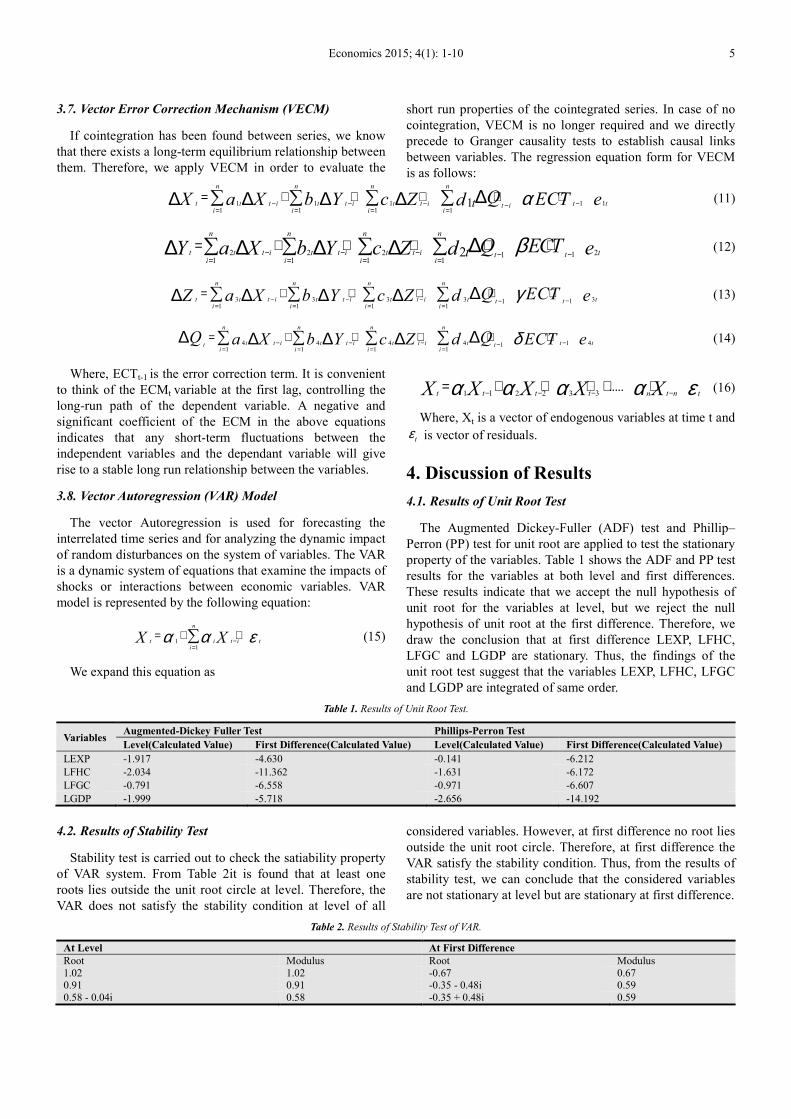
3.7. Vector Error Correction Mechanism (VECM)

If cointegration has been found between series, we know

that there exists a long-term equilibrium relationship between

them. Therefore, we apply VECM in order to evaluate the

short run properties of the cointegrated series. In case of no

cointegration, VECM is no longer required and we directly

precede to Granger causality tests to establish causal links

between variables. The regression equation form for VECM

is as follows:

1 1 1 1 11 1 1 1

1

n n n n

t t i t i t it t t t tt ii i i i

t Qa b c ECT eX X Y Z d α− − − −−= = = =

= + + + + +∆∑ ∑ ∑ ∑∆ ∆ ∆ ∆ (11)

2 2 2 2111 1 1 1

2

n n n n

t t i t i t it t t ttti i i i

t Q ECTa b c eY X Y Z d β− − − −−= = = =

= + + + + +∆∑ ∑ ∑ ∑∆ ∆ ∆ ∆ (12)

3 3 3 3 3111 1 1 1

n n n n

t t i t i t it t t t ttti i i i

Q ECTa b c d eZ X Y Z γ− − − −−= = = =

= + + + + +∆∑ ∑ ∑ ∑∆ ∆ ∆ ∆ (13)

4 4 4 4 1 411 1 1 1

n n n n

t i t i t it t t t t tt ti i i i

Q Qa b c d ECT eX Y Z δ− − − −−= = = =

= + + + + +∆ ∆∑ ∑ ∑ ∑∆ ∆ ∆ (14)

Where, ECTt-1 is the error correction term. It is convenient

to think of the ECMt variable at the first lag, controlling the

long-run path of the dependent variable. A negative and

significant coefficient of the ECM in the above equations

indicates that any short-term fluctuations between the

independent variables and the dependant variable will give

rise to a stable long run relationship between the variables.

3.8. Vector Autoregression (VAR) Model

The vector Autoregression is used for forecasting the

interrelated time series and for analyzing the dynamic impact

of random disturbances on the system of variables. The VAR

is a dynamic system of equations that examine the impacts of

shocks or interactions between economic variables. VAR

model is represented by the following equation:

11

n

t t ii ti

X Xα α ε−=

= + +∑ (15)

We expand this equation as

1 2 31 2 3.....

t t t t t nn tX X X X Xα α α α ε− − − −= + + + + + (16)

Where, Xt is a vector of endogenous variables at time t and

tε is vector of residuals.

4. Discussion of Results

4.1. Results of Unit Root Test

The Augmented Dickey-Fuller (ADF) test and Phillip–

Perron (PP) test for unit root are applied to test the stationary

property of the variables. Table 1 shows the ADF and PP test

results for the variables at both level and first differences.

These results indicate that we accept the null hypothesis of

unit root for the variables at level, but we reject the null

hypothesis of unit root at the first difference. Therefore, we

draw the conclusion that at first difference LEXP, LFHC,

LFGC and LGDP are stationary. Thus, the findings of the

unit root test suggest that the variables LEXP, LFHC, LFGC

and LGDP are integrated of same order.

Table 1. Results of Unit Root Test.

Variables Augmented-Dickey Fuller Test Phillips-Perron Test

Level(Calculated Value) First Difference(Calculated Value) Level(Calculated Value) First Difference(Calculated Value)

LEXP -1.917 -4.630 -0.141 -6.212

LFHC -2.034 -11.362 -1.631 -6.172

LFGC -0.791 -6.558 -0.971 -6.607

LGDP -1.999 -5.718 -2.656 -14.192

4.2. Results of Stability Test

Stability test is carried out to check the satiability property

of VAR system. From Table 2it is found that at least one

roots lies outside the unit root circle at level. Therefore, the

VAR does not satisfy the stability condition at level of all

considered variables. However, at first difference no root lies

outside the unit root circle. Therefore, at first difference the

VAR satisfy the stability condition. Thus, from the results of

stability test, we can conclude that the considered variables

are not stationary at level but are stationary at first difference.

Table 2. Results of Stability Test of VAR.

At Level At First Difference

Root Modulus Root Modulus 1.02 1.02 -0.67 0.67 0.91 0.91 -0.35 - 0.48i 0.59 0.58 - 0.04i 0.58 -0.35 + 0.48i 0.59


At Level At First Difference

0.58 + 0.04i 0.58 0.44 0.44 -0.29 - 0.40i 0.49 0.16 - 0.36i 0.39 -0.29 + 0.40i 0.49 0.16 + 0.36i 0.39 -0.44 0.44 0.27 0.27 0.09 0.09 -0.23 0.23 At least one root lies outside the unit circle. VAR does not satisfy the stability condition.

No root lies outside the unit circle. VAR satisfies the stability condition.

4.3. Results of Cointegration Rank Test

To determine the long run relationship among the stationary

variables Johansen cointegration test is used. Table 3 shows the

results of the cointegration test based on the maximum

eigenvalue and trace statistic test. The trace test indicates the

existence of two cointegrating equations at 1% level of

significance and the maximum eigenvalue test makes the

confirmation of this result. Thus, these results confirm that

there exist genuine long-run relationships among domestic

demand, exports and economic growth in Bangladesh.

Table 3. Results of Johansen’s Cointegration Rank Test.

Null Hypothesis Alternative

Hypothesis

Trace

Statistic

5 Percent

Critical Value

1 Percent

Critical Value

Max. Eigen

Statistic

5 Percent

Critical Value

1 Percent

Critical Value

None ** r = 1 136.01 68.52 76.07 74.49 33.46 38.77

At most 1 ** r = 2 61.51 47.21 54.46 40.49 27.07 32.24

At most 2 r = 3 21.02 29.68 35.65 15.89 20.97 25.52

At most 3 r = 4 5.14 15.41 20.04 4.83 14.07 18.63

*(**) denotes rejection of the hypothesis at the 5% (1%) level. The trace test and maximum eigenvalue test indicate 2 cointegrating equations at 5% level.

4.4. Results of Error Correction Estimation

In the short-run, there may be deviations from equilibrium

and we need to verify whether such disequilibrium converges

to the long-run equilibrium or not. Vector Error Correction

Model (VECM) can be used to check this short-run dynamics.

The estimation of a vector error correction model requires the

selection of an appropriate lag length. The number of lags in

the model has been determined according to Schawz

Information Criterion (SIC) and the appropriate lag length in

the present study is 2. Then an error correction model with

the computed-t values of the regression coefficient is

estimated and the results are presented in Table 4.

Table 4. Vector Error Correction Estimates.

Variables ∆(LGDP) ∆(LFHC) ∆(LFGC) ∆(LEXP)

Error Correction:

CointEq1

-0.190***

[-3.633]

-0.236**

[-2.055]

-1.257

[-0.952]

-0.418

[-1.372]

∆LGDP(-1) -0.558**

[-2.553]

0.590

[ 1.227]

-2.262

[-0.410]

-3.728***

[-2.923]

∆LGDP(-2) -0.172

[-1.245]

0.956***

[ 3.153]

2.020*

[1.780]

-0.691

[-0.859]

∆LFHC(-1) -0.108*

[-1.828]

-0.714***

[-3.376]

0.105*

[ 1.743]

1.218**

[ 2.173]

∆LFHC(-2) -0.137

[-1.628]

-0.406**

[-2.198]

-1.439

[-0.678]

0.222

[ 0.452]

∆LFGC(-1) 0.016*

[ 1.789]

0.030

[ 1.530]

-0.128

[-0.560]

-0.017

[-0.327]

∆LFGC(-2) 0.001*

[ 1.736]

0.030*

[ 1.700]

-0.073

[-0.365]

-0.061

[-1.308]

∆LEXP(-1) 0.050*

[ 1.900]

0.032

[ 0.462]

1.346*

[ 1.718]

-0.253

[-1.400]

∆LEXP(-2) -0.006

[-0.220]

-0.091*

[-1.920]

0.758

[ 1.027]

0.270

[ 1.586]

C 0.030

[1.358]

-0.155***

[-3.156]

-0.113

[-0.199]

0.274**

[ 2.100]

Note: The value in [ ] indicate t-value; ***, **, and * indicate 1%, 5% and

10% level of significance.

The estimated coefficient of error-correction term in the

LGDP equation is statistically significant at 1% level and has

a negative sign, which conforms that there is not any problem

in the long-run equilibrium relation between the dependent

and independent variables, but its relative value (-0.190) for

Bangladesh shows the rate of convergence to the equilibrium

state per year. Precisely, the speed of adjustment of any

disequilibrium towards a long-run equilibrium is that about

19.0% of the disequilibrium in economic growth is corrected

each year. In the second equation, i.e., in LFHC equation, the

estimated coefficient of the error term is negative and

statistically significant at 5% level. It means the error term

contribute in explaining the changes in final household

consumption.

However, in the LFGC and LEXP equations, the estimated

coefficients of the error term are negative but statistically

insignificant. As a result, the error terms do not contribute in

explaining the changes in final government consumption and

exports. Furthermore, the existence of cointegration implies

the existence of Granger causality at least in one direction

(Granger, 1988). The negative and statistically significant

value of the error correction coefficient indicates the

existence of a long-run causality between the variables of the

study. The results in Table 4 show that there exists a bi-

directional causality between final household consumption

and economic growth, but unidirectional causalities from

final government consumption to economic growth and

exports to economic growth in the long-run.

The coefficients of first difference of LFHC, first and

second differences of LFGC, and first difference of LEXP in

LGDP equation in Table 4 are statistically significant,

indicating the existence of short-run causality from final

household consumption to economic growth, final

government consumption to economic growth and export to

economic growth. In LFHC equation, the coefficient of

Economics 2015; 4(1): 1-10 7

second difference of LGDP, LFGC and LEXP are statistically

significant indicating the short-run causality from economic

growth to final household consumption, final government

consumption to final household consumption and export to

final household consumption. Again, in LFGC equation, the

coefficient of second difference of LGDP, first difference of

LFHC, and first difference of LEXP are statistically

significant, indicating the short-run causality from economic

growth, final household consumption and export to final

government consumption. Finally, in LEXP equation, the

coefficient of first difference of LGDP and LFHC are

statistically significant, indicating the existence of short-run

causality from economic growth to export and final

household consumption to export.

4.5. Results of Granger Causality Test

In order to confirm the result of short-run causality among

∆LGDP, ∆LFHC, ∆LFGC and ∆LEXP based on VECM

estimates, a standard Granger causality test has been

performed based on F-statistic. The results in Table 5 indicate

that the null hypothesis of ∆LFHC does not Granger cause

∆LGDP and ∆LGDP does not Granger cause ∆LFHC, are

rejected at 10% and 1% level of significance. Thus, in the

short-run, bi-directional causality exists between final

household consumption and economic growth. On the other

hand, the null hypothesis of ∆LFGC does not Granger cause

∆LGDP and the null hypothesis of ∆LGDP does not Granger

cause ∆LFGC, are rejected indicating that there exist short-

run bi-directional causality between economic growth final

household consumption.

The results in Table 5 also found that the null hypothesis of

∆LEXP does not Granger cause ∆LGDP and ∆LGDP does

not Granger cause ∆LEXP, are rejected at 1% level. It

indicates that there is short-run bi-directional causality

between export and economic growth. Again, the null

hypothesis of ∆LFGC does not Granger Cause ∆LFHC and

∆LFHC does not Granger Cause ∆LFGC; ∆LEXP does not

Granger Cause ∆LFHC and ∆LFHC does not Granger Cause

∆LEXP, are rejected and statistically significant, indicating

short-run bi-directional causality between government final

consumption and household final consumption; and between

export and household final consumption. Finally, the null

hypothesis of ∆LEXP does not Granger Cause ∆LFGC, is

rejected at 10% level of significance but ∆LFGC does not

Granger Cause ∆LEXP, is accepted. Therefore, in the short-

run a unidirectional causality is found between export and

government final consumption in Bangladesh. These results

support the previous results obtained from VECM about the

existence of short-run causality between the variables.

Table 5. Granger Causality Test.

Null Hypothesis Observation F-Statistic Probability Decision

∆LFHC does not Granger Cause ∆LGDP

∆LGDP does not Granger Cause ∆LFHC 39

2.707

34.246

0.081

0.000

Rejected

Rejected

∆LFGC does not Granger Cause ∆LGDP

∆LGDP does not Granger Cause ∆LFGC 39

3.096

4.307

0.057

0.021

Rejected

Rejected

∆LEXP does not Granger Cause ∆LGDP

∆LGDP does not Granger Cause ∆LEXP 39

15.594

10.064

0.000

0.001

Rejected

Rejected

∆LFGC does not Granger Cause ∆LFHC

∆LFHC does not Granger Cause ∆LFGC 39

5.491

3.226

0.009

0.053

Rejected

Rejected

∆LEXP does not Granger Cause ∆LFHC

∆LFHC does not Granger Cause ∆LEXP 39

20.418

4.566

0.000

0.018

Rejected

Rejected

∆LEXP does not Granger Cause ∆LFGC

∆LFGC does not Granger Cause ∆LEXP 39

2.723

0.188

0.080

0.829

Rejected

Accepted

Appropriate Lag: 2

4.6. Results of Vector Autoregression Model

The results of vector autoregression model are presented in

Table 6. In the present study three periods lag have been used

because LR, FEP, AIC, SC, and HQ criteria give the minimum

value in case of three periods lag which is shown in appendix

in Table A.1. Considering the LGDP equation, it is found that

one and two lag of LFHC has negative and significant effect

on LGDP, whereas two lag of LFGC and one lag of LEXP

have positive and significant effect on LGDP. In equation

LFHC, two lag of LGDP has a positive but three lag of LGDP

has negative effect on LFHC. On the other hand, only three lag

of LFGC and two lag of LEXP have positive and significant

effect on LFHC. Again, in LFGC equation, two lag of LGDP,

one lag of LFHC, two lag of export have positive and

significant effect on LFHC. In LEXP equation, one lag of

LGDP and LFGC has negative effect on LEXP where as two

lag of LGDP, one lag of LFHC, one lag of LFGC, and one and

two lag of LEXP have positive and significant effect on LEXP.

Table 6. Vector Autoregressive Analysis.

Variables LGDP LFHC LFGC LEXP

LGDP(-1) 0.400[ 2.064] 0.625[ 1.469] 1.081[ 0.193] -2.511[-1.905]

LGDP(-2) 0.438[ 2.452] 0.749[ 1.911] 7.083[ 1.708] 2.794[ 2.304]

LGDP(-3) 0.319[ 2.099] -0.710[-2.131] -1.795[-0.410] 0.616[ 0.596]

LFHC(-1) -0.201[-1.929] -0.083[-0.363] 0.121[12.100] 1.453[ 2.046]


Variables LGDP LFHC LFGC LEXP

LFHC(-2) -0.211[-1.898] -0.165[-0.674] -2.297[-0.716] -0.674[-0.891]

LFHC(-3) 0.06[ 0.556] 0.303[ 2.196] 0.473[ 0.151] -0.167[-0.226]

LFGC(-1) 0.001[ 0.106] 0.013[ 0.831] 0.542[ 2.638] -0.071[-1.868]

LFGC(-2) 0.014[ 3.500] 0.016[ 0.867] 0.055[ 0.222] -0.051[-0.875]

LFGC(-3) 0.008[ 0.851] 0.112[ 5.600] -0.034[-0.130] 0.004[ 0.062]

LEXP(-1) 0.072[ 2.446] 0.079[ 1.210] 1.091[ 3.724] 0.560[ 2.782]

LEXP(-2) -0.042[-1.346] 0.167[2.421] -0.869[-0.958] 0.390[ 1.823]

LEXP(-3) -0.011[-0.387] 0.002[ 0.027] -1.148[-1.413] -0.283[-1.475]

Constant 2.733 5.289 6.615 -18.322

Note: Value in [ ] indicates ‘t’ statistic

4.7. Results of Impulse Response Function

Impulse response functions are used to explore the

response of variables to each other in the present study.

Variables of same orders are used in the impulse response

functions because of having sensitivity. The impulse response

function is derived from the unrestricted VAR model and is

presented in Figure A.1 in Appendix A. The figure shows the

reaction of one standard deviation shock in one variable on

the other variables of the system. Assuming one standard

deviation shock in LGDP, initially the reaction is decreasing

for two periods of forecast and then it is increasing for

remaining periods. The response of LGDP to LFGC is

increasing for two periods of forecast and it is showing a

decreasing trend for reaming periods. The response result of

LGDP to LFHC shows the fluctuations for five periods and

after five periods, it shows constant trend whereas, the

response of LGDP to LEXP shows fluctuation for two

periods of forecast and for remaining periods it shows a

upward trend. The standard deviation shock in LFGC shows

the decreasing trend for whole periods of forecast. On the

other hand, the response of LEXP to LEGC indicates

decreasing trends for five periods and it increases after five

periods and becomes negative after the end of two periods.

Again, the responses of LFHC to LGDP, LFHC to LFGC,

LFHC to LEXP and LFGC to LGDP show upward trend for

whole forecast periods whereas the response of LFGC to

LFHC shows nearly constant trend for all periods of forecast.

The standard deviation shock in LFHC indicates fluctuation

for five periods of forecast and it shows decreasing trends for

remaining periods of forecast. The trends of response of

LEXP to LFHC and LEXP to LGDP fluctuate for three

periods and become upward after three periods whereas the

response of LFGC to LEXP fluctuates for eight periods and

become constant after eight periods

5. Conclusion and Policy Suggestions

The present study has explored the causal relationship

between domestic demand, exports and economic growth in

the context of Bangladesh using data on real GDP, real

exports, final household consumption and final government

consumption over the period 1971–2011. The results of the

tests suggest that a positive long-run equilibrium relationship

exists among domestic demand, exports and economic

growth. There has been a significant bidirectional

relationship between final household consumption and

economic growth, and a significant unidirectional

relationship running from final government consumption to

economic growth and export to economic growth for

Bangladesh during the study period. The findings of causal

relationship between domestic demand, export and economic

growth support both the domestic demand-based and the

export-led growth in Bangladesh. Thus, it can be concluded

that a successful and sustained economic growth need

enough domestic demand. Moreover, direct effect of exports

on growth means that exports affect economic growth.

Therefore, it should be clear from Bangladesh’s case that

domestic demand and export sustain the country’s long-run

economic growth. Therefore, the government of Bangladesh

should come forward with proper domestic demand and

export oriented policies, and act properly to promote exports

and domestic demand.

Appendix A

Table A. 1. VAR Lag Order Selection Criterion.

Lag LogL LR FPE AIC SC HQ

0 124.48 NA 1.28E-09 -6.29 -6.07 -6.21

1 405.79 473.78 1.79E-15 -19.78 -18.49 -19.32

2 471.61 93.54 2.25E-16 -21.93 -19.56 -21.08

3 547.34 87.69* 1.89E-17* -24.59* -21.15* -23.37*

*indicates lag order selected by the criterion: LR = Sequential modified LR test statistic; FPE = Final prediction error; AIC = Akiake information criterion; SC

= Schwarz information criterion; HQ = Hannan-Quinn information criterion.

Economics 2015; 4(1): 1-10 9

Figure A. 1. Impulse Response Functions.

References

[1] Abu, Stait, F. 2005. Are Exports the Engine of Economic Growth? An Application of Cointegration and Causality Analysis for Egypt, 1977-2003. Economic Research, Working Paper Series.

[2] Ahmed, H.A., Uddin, M.G.S.2009.Export, Imports, Remittance and Growth in Bangladesh: An Empirical Analysis, Trade and Development Review, 2(2), 79-92.

[3] Al Mamun, K. A., Nath H. K. (2005). Export-led growth in Bangladesh: A Time Series Analysis. Applied Economics Letters, 12, 361–364.

[4] Asian Development Bank (ADB).2005. Asian Development Outlook, 2005, Asia Development Bank.

[5] Bangladesh Bank (BB). 2012. Major Economic Indicator, Monthly Update. Monetary Policy Department, Bangladesh Bank, Volume: 08/2013, August 2013.

[6] Bangladesh Bureau of Statistics (BBS). 2002. Statistical Yearbook of Bangladesh, Ministry of Planning, Dhaka.

[7] Bangladesh Bureau of Statistics (BBS). 2012. Statistical Yearbook of Bangladesh, Ministry of Planning, Dhaka.

[8] Central Intelligence Agency (CIA), 2011. World Fact Book, Retrieved 2011-01-04.

[9] Chimobi, Philip, Uche, O., Charles, U. 2010. Export, Domestic Demand and Economic Growth in Nigeria: Granger Causality Analysis. European Journal of Social Sciences, 13(2), 2-11

[10] Engle, R.F., Granger C.W.J., 1987. Cointegration and Error Correction Representation, Estimation and Testing”, Econometrica, 55, 1-87.

[11] Export Promotion Bureau (EPB).2012. Bangladesh Export Statistics. Information Division of Export Promotion Bureau, Ministry of Commerce, Bangladesh.

-.01

.00

.01

.02

.03

.04

1 2 3 4 5 6 7 8 9 10

Response of LFHC to LFHC

-.01

.00

.01

.02

.03

.04

1 2 3 4 5 6 7 8 9 10

Response of LFHC to LGDP

-.01

.00

.01

.02

.03

.04

1 2 3 4 5 6 7 8 9 10

Response of LFHC to LFGC

-.01

.00

.01

.02

.03

.04

1 2 3 4 5 6 7 8 9 10

Response of LFHC to LEXP

-.01

.00

.01

.02

1 2 3 4 5 6 7 8 9 10

Response of LGDP to LFHC

-.01

.00

.01

.02

1 2 3 4 5 6 7 8 9 10

Response of LGDP to LGDP

-.01

.00

.01

.02

1 2 3 4 5 6 7 8 9 10

Response of LGDP to LFGC

-.01

.00

.01

.02

1 2 3 4 5 6 7 8 9 10

Response of LGDP to LEXP

-.2

-.1

.0

.1

.2

.3

.4

.5

1 2 3 4 5 6 7 8 9 10

Response of LFGC to LFHC

-.2

-.1

.0

.1

.2

.3

.4

.5

1 2 3 4 5 6 7 8 9 10

Response of LFGC to LGDP

-.2

-.1

.0

.1

.2

.3

.4

.5

1 2 3 4 5 6 7 8 9 10

Response of LFGC to LFGC

-.2

-.1

.0

.1

.2

.3

.4

.5

1 2 3 4 5 6 7 8 9 10

Response of LFGC to LEXP

-.08

-.04

.00

.04

.08

.12

1 2 3 4 5 6 7 8 9 10

Response of LEXP to LFHC

-.08

-.04

.00

.04

.08

.12

1 2 3 4 5 6 7 8 9 10

Response of LEXP to LGDP

-.08

-.04

.00

.04

.08

.12

1 2 3 4 5 6 7 8 9 10

Response of LEXP to LFGC

-.08

-.04

.00

.04

.08

.12

1 2 3 4 5 6 7 8 9 10

Response of LEXP to LEXP

Response to Cholesky One S.D. Innovations ± 2 S.E.


[12] Felipe, J., Lim J.A. 2005. Export or Domestic-led Growth in Asia? Asian Development Review, 22(2), 35-75.

[13] Granger C.W. J. 1969.Investing causal relations by econometric models and cross-spectral methods. Econometrica, 37(3), 424-438.

[14] Johansen, S. 1988. Statistical Analysis of Cointegration Vectors. Journal of Economic Dynamics and Control, 12, 231-254.

[15] Wah L. Y. 2010. The role of domestic demand in the economic growth of Malaysia: a cointegration analysis. International Economic Journal, 18(3), 337-352.

[16] Ramos, F.F.R. 2000. Exports, imports, and economic growth in Portugal: evidence from causality and cointegration analysis. Journal of Economic Modeling, 18, 613-623.

[17] Tesen, H.W., 2007. Export Domestic Demand and Economic Growth: Some Empirical Evidence of Middle East Countries. Journal of Economic Cooperation, 28(2), 52-82.

[18] Wong, H. T. 2008. Exports and Domestic Demand: Some Empirical Evidence in Asean-5.Labuan Bulletin of International Business & Finance, 6, 39-55.

Domestic demand, export and economic growth in Bangladesh: A cointegration and VECM approach

Documents

Transcript of Domestic demand, export and economic growth in Bangladesh: A cointegration and VECM approach