A Survey of Cloud Lighting and Rendering Techniques

Roland HufnagelUniv. Salzburg, Salzburg, Austria

rhufna@cosy.sbg.ac.at

Martin HeldUniv. Salzburg, Salzburg, Austria

held@cosy.sbg.ac.at

ABSTRACTThe rendering of participating media still forms a big challenge for computer graphics. This remark is particularlytrue for real-world clouds with their inhomogeneous density distributions, large range of spatial scales and differentforms of appearance. We survey techniques for cloud visualization and classify them relative to the type of volumerepresentation, lighting and rendering technique used. We also discuss global illumination techniques applicableto the generation of the optical effects observed in real-world cloud scenes.

Keywordscloud rendering, cloud lighting, participating media, global illumination, real-world clouds

1 INTRODUCTION

We review recent developments in the rendering of par-ticipating media for cloud visualization. An excellentsurvey on participating media rendering was presentedby Cerezo et al. [5] a few years ago. We build upontheir survey and present only recently published tech-niques, with a focus on the rendering of real-worldcloud scenes. In addition, we discuss global illumina-tion techniques for modeling cloud-to-cloud shadowsor inter-reflection.

We start with explaining real-world cloud phenomena,state the graphics challenges caused by them, and moveon to optical models for participating media. In thefollowing sections we categorize the state-of-the-art ac-cording to three aspects: The representation of clouds(Section 2), rendering techniques (Section 3) and light-ing techniques (Section 4).

1.1 Cloud PhenomenologyClouds exhibit a huge variety of types, differing accord-ing to the following aspects.

Size: Clouds reside in the troposphere, which is thelayer above the Earth’s surface reaching up to heightsof 9–22 km. In the mid-latitudes clouds show a maxi-mum vertical extension of 12–15 km. Their horizontalextension reaches from a few hundred meters (Fig. 1.7)to connected cloud systems spanning thousands of kilo-meters (Figs. 1.11 and 1.12).

Permission to make digital or hard copies of all or part ofthis work for personal or classroom use is granted withoutfee provided that copies are not made or distributed for profitor commercial advantage and that copies bear this notice andthe full citation on the first page. To copy otherwise, or re-publish, to post on servers or to redistribute to lists, requiresprior specific permission and/or a fee.

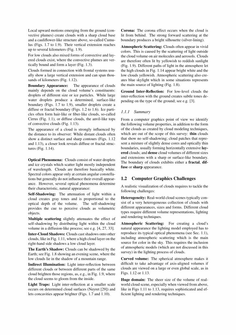
Figure 1: Clouds as seen from the ground: broken cloudlayers with fractal cloud patches (top row), clouds withdiffuse boundaries (second row), dense cloud volumeswith surface-like boundaries (third row); and cloudsviewed from a plane and from space (last two rows),where (14) shows a zoom into the central region of (13).

Geometry: In relation to the Earth’s radius (6371 km)the troposphere represents a shallow spherical shell.The curvature of the Earth produces the horizon and isdirectly visible when viewing clouds from space.

Clouds often develop at certain heights and form layers.These either consist of cloud patches (Fig. 1.1 to 1.5) orcreate overcast cloud sheets (Fig. 1.6 or 1.11).

Local upward motions emerging from the ground (con-vective plumes) create clouds with a sharp cloud baseand a cauliflower-like structure above, so-called Cumu-lus (Figs. 1.7 to 1.9). Their vertical extension reachesup to several kilometers (Fig. 1.9).For low clouds also mixed forms of convective and lay-ered clouds exist, where the convective plumes are ver-tically bound and form a layer (Fig. 1.3).Clouds formed in connection with frontal systems usu-ally show a large vertical extension and can span thou-sands of kilometers (Fig. 1.12).Boundary Appearance: The appearance of cloudsmainly depends on the cloud volume’s constituents:droplets of different size or ice particles. While largewater droplets produce a determined, surface-likeboundary (Figs. 1.7 to 1.9), smaller droplets create adiffuse or fractal boundary (Figs. 1.2 to 1.6). Ice parti-cles often form hair-like or fiber-like clouds, so-calledCirrus (Fig. 1.1), or diffuse clouds, the anvil-like topsof convective clouds (Fig. 1.13).The appearance of a cloud is strongly influenced bythe distance to its observer: While distant clouds oftenshow a distinct surface and sharp contours (Figs. 1.12and 1.13), a closer look reveals diffuse or fractal struc-tures (Fig. 1.14).

Optical Phenomena: Clouds consist of water dropletsand ice crystals which scatter light mostly independentof wavelength. Clouds are therefore basically white.Spectral colors appear only at certain angular constella-tions but generally do not influence their overall appear-ance. However, several optical phenomena determinetheir characteristic, natural appearance:Self-Shadowing: The attenuation of light within acloud creates gray tones and is proportional to theoptical depth of the volume. The self-shadowingprovides the cue to perceive clouds as volumetricobjects.Multiple scattering slightly attenuates the effect ofself-shadowing by distributing light within the cloudvolume in a diffusion-like process; see e.g. [4, 27, 33].Inter-Cloud Shadows: Clouds cast shadows onto otherclouds, like in Fig. 1.11, where a high cloud layer on theright-hand side shadows a low cloud layer.The Earth’s Shadow: Clouds can be shadowed by theEarth; see Fig. 1.8 showing an evening scene, where thelow clouds lie in the shadow of a mountain range.Indirect Illumination: Light inter-reflection betweendifferent clouds or between different parts of the samecloud brighten those regions, as, e.g., in Fig. 1.9, wherethe cloud seems to gloom from the inside.Light Traps: Light inter-reflection at a smaller scaleoccurs on determined cloud surfaces (Neyret [29]) andlets concavities appear brighter (Figs. 1.7 and 1.10).

Corona: The corona effect occurs when the cloud islit from behind. The strong forward scattering at theboundary produces a bright silhouette (silver-lining).

Atmospheric Scattering: Clouds often appear in vividcolors. This is caused by the scattering of light outsidethe cloud volume on air molecules and aerosols. Cloudsare therefore often lit by yellowish to reddish sunlight(Fig. 1.9). Different paths of light in the atmosphere letthe high clouds in Fig. 1.14 appear bright white and thelow clouds yellowish. Atmospheric scattering also cre-ates blue skylight which in some situations representsthe main source of lighting (Fig. 1.8).

Ground Inter-Reflection: For low-level clouds theinter-reflection with the ground creates subtle tones de-pending on the type of the ground; see e.g. [3].

1.1.1 Summary

From a computer graphics point of view we identifythe following volume properties, in addition to the formof the clouds as created by cloud modeling techniques,which are out of the scope of this survey: thin cloudsthat show no self-shadowing; cloud patches that repre-sent a mixture of slightly dense cores and optically thinboundaries, usually forming horizontally extensive lay-ered clouds; and dense cloud volumes of different sizesand extensions with a sharp or surface-like boundary.The boundary of clouds exhibits either a fractal, dif-fuse or sharp appearance.

1.2 Computer Graphics ChallengesA realistic visualization of clouds requires to tackle thefollowing challenges:

Heterogeneity: Real-world cloud scenes typically con-sist of a very heterogeneous collection of clouds withdifferent appearances, sizes and forms. Different cloudtypes require different volume representations, lightingand rendering techniques.

Atmospheric Scattering: For creating a cloud’snatural appearance the lighting model employed has toreproduce its typical optical phenomena (see Sec. 1.1),including atmospheric scattering which is the mainsource for color in the sky. This requires the inclusionof atmospheric models (which are not discussed in thissurvey) in the lighting process of clouds.

Curved volume: The spherical atmosphere makes itdifficult to take advantage of axis-aligned volumes ifclouds are viewed on a large or even global scale, as inFigs. 1.12 or 1.13.

Huge domain: The sheer size of the volume of real-world cloud scene, especially when viewed from above,like in Figs 1.11 to 1.13, requires sophisticated and ef-ficient lighting and rendering techniques.

1.3 Participating MediaA cloud volume constitutes a participating medium ex-hibiting light attenuation and scattering. This sectionuses the terminology of [5] to provide a short introduc-tion to the radiometry of participating media.

While light in vacuum travels along straight lines, thisis not the case for participating media. Here photons in-teract with the medium by being scattered or absorbed.From a macroscopic point of view light spreads in par-ticipating media, gets blurred and attenuated, similar toheat diffusion in matter.

Participating media are characterized by a particle den-sity ρ , an absorption coefficient κa, a scattering coeffi-cient κs, and a phase function p(~ω, ~ω ′) which describesthe distribution of light after scattering.

Absorption is the process where radiation is trans-formed to heat. The attenuation of a ray of light withradiance L and direction ~ω at position x (within an in-finitesimal ray segment) is described by

(~ω ·∇)L(x, ~ω) = −κa(x)L(x, ~ω).

In the atmosphere absorption is mainly due to water va-por and aerosols. Cloud droplets or ice crystals showlittle absorption which means that the light distributionin clouds is dominated by scattering.

Scattering is the process where radiance is absorbedand re-emitted into other directions. Out-scatteringrefers to the attenuation of radiance along direction ~ωdue to scattering into other directions:

(~ω ·∇)L(x, ~ω) =−κs(x)L(x, ~ω).

In-scattering refers to the scattering of light into thedirection ~ω from all directions (integrated over thesphere) at a point x:

(~ω ·∇)L(x, ~ω) =κs(x)4π

∫4π

p(~ω ′, ~ω)L(x, ~ω ′)dω′,

Extinction is the net effect of light attenuation due to ab-sorption and out-scattering described by the extinctioncoefficient κt = κa +κs.

Emission contributes light to a ray:

(~ω ·∇)L(x, ~ω) = κa(x)Le(x, ~ω).

It is usually not relevant for cloud rendering sinceclouds do not emit light. (An exception is lightninginside a cloud.)

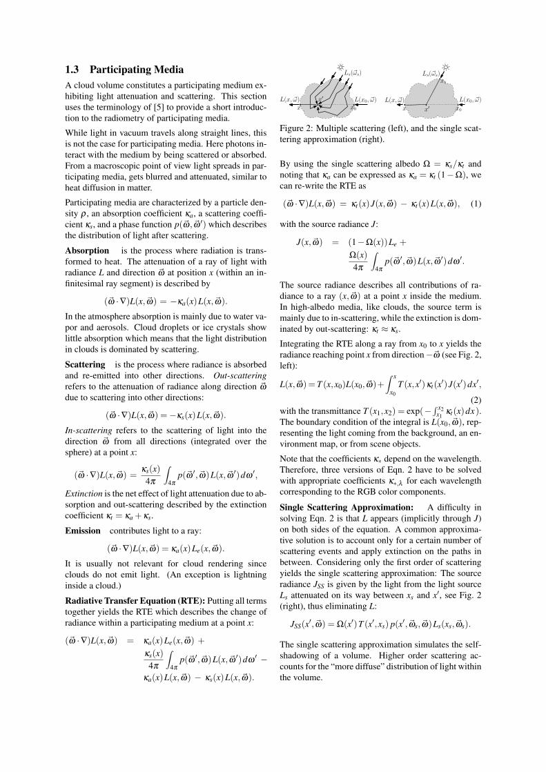
Radiative Transfer Equation (RTE): Putting all termstogether yields the RTE which describes the change ofradiance within a participating medium at a point x:

(~ω ·∇)L(x, ~ω) = κa(x)Le(x, ~ω) +

κs(x)4π

∫4π

p(~ω ′, ~ω)L(x, ~ω ′)dω′ −

κa(x)L(x, ~ω) − κs(x)L(x, ~ω).

L(x, ~ω) L(x0, ~ω)x′

x x0

Ls(~ωs)

L(x, ~ω) L(x0, ~ω)

x′x x0

xsLs(~ωs)

Figure 2: Multiple scattering (left), and the single scat-tering approximation (right).

By using the single scattering albedo Ω = κs/κt andnoting that κa can be expressed as κa = κt (1−Ω), wecan re-write the RTE as

(~ω ·∇)L(x, ~ω) = κt(x)J(x, ~ω) − κt(x)L(x, ~ω), (1)

with the source radiance J:

J(x, ~ω) = (1−Ω(x))Le +

Ω(x)4π

∫4π

p(~ω ′, ~ω)L(x, ~ω ′)dω′.

The source radiance describes all contributions of ra-diance to a ray (x, ~ω) at a point x inside the medium.In high-albedo media, like clouds, the source term ismainly due to in-scattering, while the extinction is dom-inated by out-scattering: κt ≈ κs.

Integrating the RTE along a ray from x0 to x yields theradiance reaching point x from direction−~ω (see Fig. 2,left):

L(x, ~ω)= T (x,x0)L(x0, ~ω)+∫ x

x0

T (x,x′)κt(x′)J(x′)dx′,

(2)with the transmittance T (x1,x2) = exp(−∫ x2

x1κt(x)dx).

The boundary condition of the integral is L(x0, ~ω), rep-resenting the light coming from the background, an en-vironment map, or from scene objects.

Note that the coefficients κ∗ depend on the wavelength.Therefore, three versions of Eqn. 2 have to be solvedwith appropriate coefficients κ∗,λ for each wavelengthcorresponding to the RGB color components.

Single Scattering Approximation: A difficulty insolving Eqn. 2 is that L appears (implicitly through J)on both sides of the equation. A common approxima-tive solution is to account only for a certain number ofscattering events and apply extinction on the paths inbetween. Considering only the first order of scatteringyields the single scattering approximation: The sourceradiance JSS is given by the light from the light sourceLs attenuated on its way between xs and x′, see Fig. 2(right), thus eliminating L:

JSS(x′, ~ω) = Ω(x′)T (x′,xs) p(x′, ~ωs, ~ω)Ls(xs, ~ωs).

The single scattering approximation simulates the self-shadowing of a volume. Higher order scattering ac-counts for the “more diffuse” distribution of light withinthe volume.

Phase Function: A scattering phase function is a prob-abilistic description of the directional distribution ofscattered light. Generally it depends on the wavelength,and the form and size of the particles in a medium. Usu-ally phase functions show a symmetry according to theincident light direction, which reduces it to a functionof the angle θ between incident and exitant light p(θ).

Often approximations for certain types of scattering areused, like the Henyey-Greenstein or the Schlick func-tion. However, as noted in [4], those functions cannotmodel visual effects that depend on small angular vari-ations, like glories or fog-bows. See [4] and its refer-ences for plots and tabular listings of phase functions.

2 CLOUD REPRESENTATIONSA cloud representation specifies the spatial distribution,overall structure, form, and boundary appearance ofclouds in a cloud scene.

2.1 Hierarchical Space Subdivision2.1.1 Voxel Octrees

Voxel octrees are a hierarchical data structure built upona regular grid by collapsing the grid cells of a 2×2×2cube (children) to a single voxel (parent).

Sparse voxel octrees reduce the tree size by account-ing for visibility and LOD: Interior voxels are removed,yielding a hull- or shell-like volume representation (seeFig. 3, middle). Also hidden voxels (relative to the cur-rent viewing point) are removed (see Fig. 3, right). Ad-ditionally the LOD resolution can be limited accordingto the screen resolution (view-dependent LOD). Thesetechniques require an adaptive octree representation ac-companied with an update strategy.

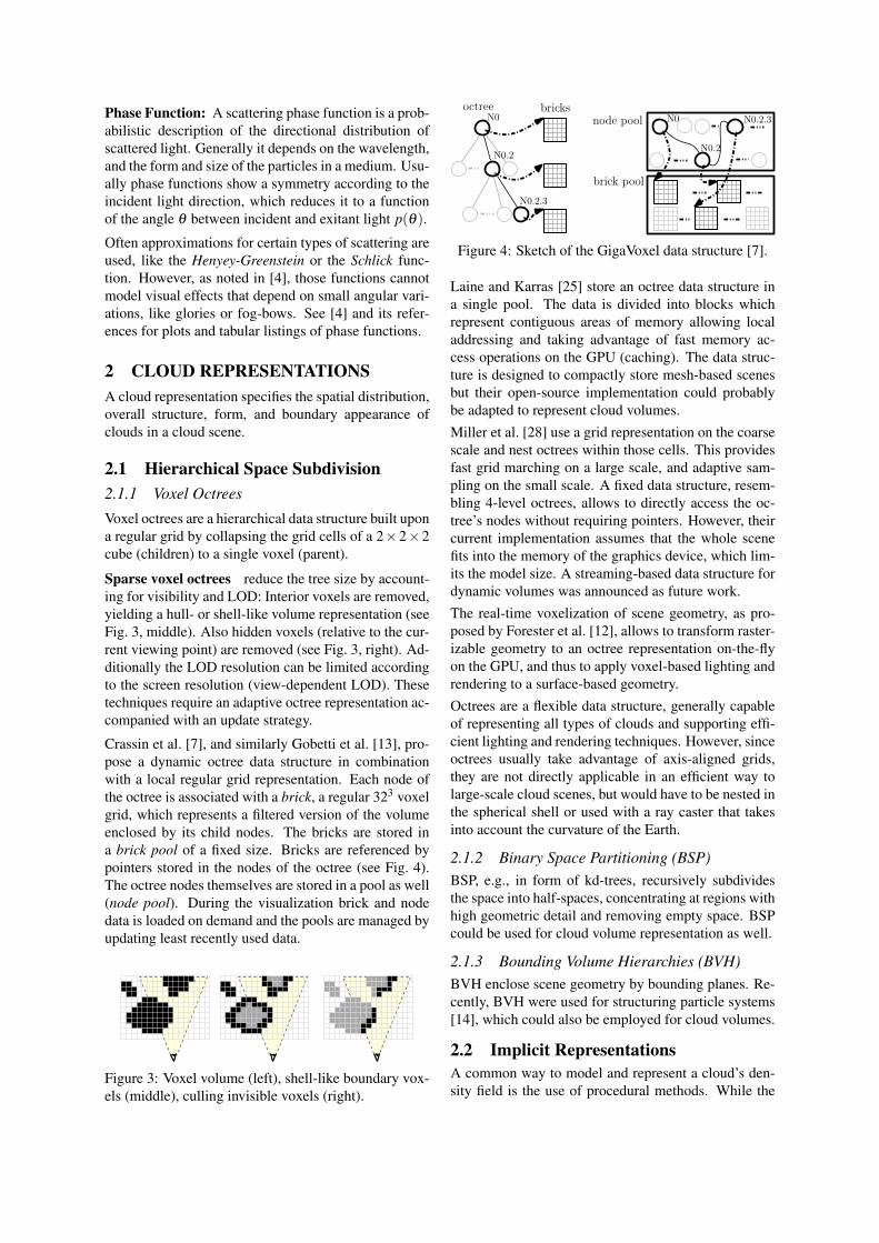
Crassin et al. [7], and similarly Gobetti et al. [13], pro-pose a dynamic octree data structure in combinationwith a local regular grid representation. Each node ofthe octree is associated with a brick, a regular 323 voxelgrid, which represents a filtered version of the volumeenclosed by its child nodes. The bricks are stored ina brick pool of a fixed size. Bricks are referenced bypointers stored in the nodes of the octree (see Fig. 4).The octree nodes themselves are stored in a pool as well(node pool). During the visualization brick and nodedata is loaded on demand and the pools are managed byupdating least recently used data.

Figure 3: Voxel volume (left), shell-like boundary vox-els (middle), culling invisible voxels (right).

N0

N0.2

N0.2.3

brick pool

N0.2.3

N0.2

N0node pooloctree bricks

Figure 4: Sketch of the GigaVoxel data structure [7].

Laine and Karras [25] store an octree data structure ina single pool. The data is divided into blocks whichrepresent contiguous areas of memory allowing localaddressing and taking advantage of fast memory ac-cess operations on the GPU (caching). The data struc-ture is designed to compactly store mesh-based scenesbut their open-source implementation could probablybe adapted to represent cloud volumes.Miller et al. [28] use a grid representation on the coarsescale and nest octrees within those cells. This providesfast grid marching on a large scale, and adaptive sam-pling on the small scale. A fixed data structure, resem-bling 4-level octrees, allows to directly access the oc-tree’s nodes without requiring pointers. However, theircurrent implementation assumes that the whole scenefits into the memory of the graphics device, which lim-its the model size. A streaming-based data structure fordynamic volumes was announced as future work.The real-time voxelization of scene geometry, as pro-posed by Forester et al. [12], allows to transform raster-izable geometry to an octree representation on-the-flyon the GPU, and thus to apply voxel-based lighting andrendering to a surface-based geometry.Octrees are a flexible data structure, generally capableof representing all types of clouds and supporting effi-cient lighting and rendering techniques. However, sinceoctrees usually take advantage of axis-aligned grids,they are not directly applicable in an efficient way tolarge-scale cloud scenes, but would have to be nested inthe spherical shell or used with a ray caster that takesinto account the curvature of the Earth.

2.1.2 Binary Space Partitioning (BSP)BSP, e.g., in form of kd-trees, recursively subdividesthe space into half-spaces, concentrating at regions withhigh geometric detail and removing empty space. BSPcould be used for cloud volume representation as well.

2.1.3 Bounding Volume Hierarchies (BVH)BVH enclose scene geometry by bounding planes. Re-cently, BVH were used for structuring particle systems[14], which could also be employed for cloud volumes.

2.2 Implicit RepresentationsA common way to model and represent a cloud’s den-sity field is the use of procedural methods. While the

Figure 5: Perlin noise [31] and “fractal sum” [11] func-tions (left). A hypertexture applied to a surface (right).

overall structure is usually specified by simple geomet-ric primitives, like spheres or ellipsoids, the internal,high-resolution structure is modeled by a function.

Perlin and Hoffert [31] introduce space-filling shapes,based on procedural functions, so-called hypertextures.Ebert et al. [11] propose many additional noise func-tions (see Fig. 5, left), and create various natural pat-terns applicable also for clouds.

The sampling of implicitly defined densities can be-come expensive and harm rendering performance. Sch-pok et al. [36] propose to evaluate the procedural func-tions on-the-fly on the GPU during the rendering by us-ing a fragment shader program and a 3D texture con-taining Perlin noise.

Kniss et al. [22] use procedural functions for geomet-ric distortion which adds a fractal appearance to regularshapes by changing the vertex positions of the geometryrendered. They apply this distortion during the render-ing process by using vertex shader programs.

Bouthors et al. [4] use hypertextures in combinationwith surface-bounding volumes for creating a fractalboundary appearance; see Fig. 5, right.

Implicitly specifying a volume via procedural functionsis a compact volume representation. The computationalcost can be mitigated by employing parallel process-ing on the GPU and taking advantage of hardware-supported tri-linear interpolation of 3D textures. Pro-cedural techniques are perfect for clouds with a frac-tal boundary appearance. However, they only providethe fine-scale volume structure while the overall cloudshape has to be modeled by other techniques.

2.3 Particle SystemsThe volume is represented by a set of particles with apre-defined volume. Usually spherical particles with aradial density function are used.

Nishita et al. [30] promote the use of particles witha Gaussian density distribution, so-called metaballs.While the metaballs in [30] are used only to create avolume density distribution, Dobashi et al. [10] directlylight and render the metaballs and visualize medium-size cloud scenes of Cumulus-like clouds with a diffuseboundary appearance.

Bouthors and Neyret [2] use particles to create a shell-like volume representation for Cumulus-like clouds.

Their algorithm iteratively places particles at the in-terface of a cloud volume, with smaller particles beingplaced upon the interface of larger particles. This cre-ates a hierarchy of particles with decreasing radius andspecifies the cloud’s surface, which can be transformed,e.g., to a triangle mesh.

Efficient transformation algorithms were developed tomatch the favored lighting and rendering approaches.Cha et al. [6] transform the density distribution givenby a particle system to a regular grid by using the GPU,while Zhou et al. [44] propose the inverse process trans-forming a density field to radial basis function (RBF)representation. This low-resolution particle system isaccompanied by a high-resolution grid, which storesdeviations of the particles’ density distribution from theinitial density field in a so-called residual field. Perfectspatial hashing allows a compact storage of this field.

Particles systems are a compact volume representationand directly support many cloud modeling techniques.Spherical particles are well suited for Cumulus-likeclouds or dense cloud volumes, but less appropriate forstratified cloud layers with a large horizontal extensionor for thin, fiber-like clouds.

2.4 Surface-Bounded VolumesThe cloud volume is represented by its enclosing hull,usually given as a triangle mesh. Since no informationon the internal structure is available, usually a homoge-neous volume is assumed.

Bouthors et al. [4] demonstrate the use of surface-bounded volumes for visualizing single Cumulusclouds. A triangle mesh is used in combinationwith a hypertexture to add small-scale details at theboundaries. A sophisticated lighting model reproducesa realistic appearance (see Sec. 4.1.4).

Porumbescu et al. [32] propose shell maps to create avolumetric texture space on a surface. A tetrahedralmesh maps arbitrary volumetric textures to this shell.

Surface-bounded volumes are a very compact represen-tation of cloud volumes, allowing for efficient renderingand for incorporating sophisticated lighting techniques.However, they are only applicable if a quick saturationof a ray entering the volume may be assumed. Whilethis is valid for dense clouds it does not apply to thinor layered clouds with their optically thin boundaries.Also special rendering techniques have to be developedfor allowing perspectives from within the clouds.

2.5 Clouds as LayersClouds represented by a single layer, usually renderedas a textured triangle mesh, allow fast rasterization-based rendering and are the traditional technique topresent clouds, e.g., during weather presentations [24].

Bouthors et al. [3] visualize cloud layers viewed fromthe ground or from above. They achieve a realisticappearance of the cloud by applying a sophisticated,viewpoint-dependent lighting model.

The 2D representation is especially predestined for thincloud sheets viewed from the ground, or for visualizingthe cloud tops viewed, e.g., from the perspective of asatellite. However, this non-volumetric representationlimits the possible perspectives and generally does notallow for animations, like transitions of the viewpointfrom space to the ground, or cloud fly-throughs.

3 CLOUD RENDERING TECHNIQUES3.1 Rasterization-based Rendering3.1.1 Volume SlicingVolume slicing is a straightforward method for render-ing regular grids. The slices are usually axis alignedand rendered in front-to-back order (or vice-versa), ap-plying viewing transformations and blending. Whilevolume slicing is not necessarily a rasterization-basedmethod, most algorithms exploit the highly optimizedtexturing capabilities of the graphics hardware.

Schpok et al. [36] use volume slicing for cloud render-ing and propose the use of the GPU also for adding de-tailed cloud geometry on-the-fly by using a fragmentshader program. This reduces the amount of data whichhas to be transferred onto the GPU to a low-resolutionversion of the cloud volume. Harris et al. [15] createthe density volume by a CFD simulation on the GPUfor creating a 3D density and light texture which canefficiently be rendered on the GPU. Sparing the trans-fer of the volumetric data from the CPU, they achieveinteractive frame rates for small volumes (up to 643),creating soft, diffuse clouds. Hegeman et al. [17] alsouse 3D textures to capture the volume density and thepre-calculated source radiance, and evaluate a lightingmodel in a CG shader program during rendering.

Zhou et al. [44] visualize smoke represented by alow-resolution particle system accompanied by ahigh-resolution density grid, stored in compressedform (see Sec. 2.3). During the rendering process thelighted particles are first rasterized and converted to a3D texture by applying parallel projection renderingalong the z-axis to fill slices of the 3D texture. Thereby,for each slice, all particles are traversed and, in caseof intersection with the slicing plane, rendered astextured quads. During this pass also the residualfield is evaluated and stored in a separate 3D texture.In a second step perspective rendering is applied byslicing in back-to-front manner. Again, for each sliceall particles are traversed and bounding quads arerendered triggering a fragment shader which composesthe light and density information from the 3D textures.They achieve interactive frame rates under dynamic

Figure 6: Volume rendering by half-angle slicing.

lighting conditions for moderate volume sizes whichcompletely fit into the GPU’s memory (1283 in theirexamples), based on 0.5 to 1.5 hours of pre-processingtime.Half-Angle Slicing: Slicing the volume at planes ori-ented halfway between the lighting and viewing direc-tion (or its inverse, see Fig. 6) is called half-angle slic-ing. It allows to combine the lighting and rendering ofthe volume in a single process by iterating once overall slices. During this single-volume pass two buffersare maintained and iteratively updated: one for accumu-lating the attenuation of radiance in the light direction,and one for accumulating the radiance for the observer(usually in the frame buffer). Due to the single passthrough the volume, the lighting scheme is limited toeither forward or backward scattering.Kniss et al. [22] use half-angle slicing in combinationwith geometric distortion, modifying the geometry ofshapes on-the-fly during rendering (see Sec. 2.2) by us-ing vertex shader programs. Riley et al. [35] visualizethunderstorm clouds, taking into account different scat-tering properties of the volume.For avoiding slice-like artifacts volume slicing tech-niques have to employ small slicing intervals, resultingin a large number of slices which can harm renderingperformance and introduce numerical problems. Inho-mogeneous volumes, like in Figs. 1.2 or 1.14, wouldalso require a huge number of slices for appropriatelycapturing the volume’s geometry and avoiding artifactsin animations with a moving viewpoint. Slicing-basedmethods therefore seem to favor volumes with soft ordiffuse boundaries and, thus, are applicable to cloudswith sharp boundaries only to a limited extent.

3.1.2 SplattingSplatting became the common method for renderingparticle systems. Particles, which are usually specifiedas independent of rotation, can be rendered by using atextured quad representing the projection of the particleonto a plane, also called splat or footprint. The particlesare rendered in back-to-front order, applying blendingfor semi-transparent volumes.Dobashi et al. [10] use metaballs for splatting cloudvolumes. Harris et al. [16] accelerate this approachby re-using impostors, representing projections of aset of particles, for several frames during fly-throughs.The use of different particle textures can enhance theclouds’ appearance [42, 18].

Since usually a single color (or luminance) is assignedto each particle and the particles do not represent a dis-tinct geometry, but a spherical, diffuse volume (due tothe lack of self-shadowing within a particle), the splat-ting approach is limited to visualizing clouds with asoft, diffuse appearance. Clouds with a distinct surfacegeometry, like Cumulus clouds, cannot be reproducedrealistically.

3.1.3 Surface-Based Volume Rendering

Nowadays, rendering clouds as textured ellipsoids isno more regarded as realistic. The same applies to thesurface-bounded clouds of [41]. A triangle mesh is cre-ated by surface subdivision of an initial mesh, createdby a marching cubes algorithm applied on weather fore-cast data. The rendering of the semi-transparent mesh,however, is prone to artifacts on the silhouette.

Bouthors et al. [4] resurrected surface-based cloud ren-dering by using fragment shader programs which cal-culate the color for each fragment of a triangle meshat pixel-basis. This allows to apply a sophisticatedvolume lighting scheme and the sampling of a hyper-texture superposed onto the surface on-the-fly for eachpixel. They achieve a realistic, real-time visualizationof dense clouds with fractal and sharp boundaries.

3.2 Ray Casting-Based Rendering3.2.1 Ray Marching

Ray marching casts rays into the scene and accumulatesthe volume densities at certain intervals. For renderingparticipating media volumes, like clouds, the illumina-tion values of the volume have to be evaluated, eitherby applying a volume lighting model on-the-fly or byretrieving the illumination from a pre-computed light-ing data structure.

Grids: Cha et al. [6] transform a particle-based volumerepresentation to a regular density grid for applying raymarching. The volume density is sampled within a 3Dtexture, combined with the illumination, stored in a sep-arate 3D texture, and accumulated along the viewingrays. Geometric detail is added to the low-resolutionvolume representation on-the-fly by slightly distortingthe sampling points of the ray march according to a pre-computed 3D procedural noise texture. For volumes fit-ting into the memory of the GPU (around 2563 in theirexamples), they achieve rendering times of a few sec-onds (including the lighting calculation).

BVHs: A particle system stored within a kd-treestructure is proposed by Gourmel et al. [14] for fast raytracing. The technique could be used for cloud render-ing, e.g., by ray marching through the particle volumesand adding procedural noise as proposed in [4] or [6].

Octrees: The huge amount of data caused by volu-metric representations can be substantially reduced byusing ray-guided streaming [7, 13, 25]. The GigaVoxelalgorithm [7] is based on an octree with associatedbricks (Sec. 2.1.1) which are maintained in a pool andstreamed on demand. The bricks at different levels ofthe octree represent a multi-resolution volume, similarto a mip-map texture. Sampling densities at differentmip-map resolutions simulates cone tracing (see Fig. 4,right). The octree is searched in a stack-less manner,always starting the search for a sampling position at theroot node. This supports the cone-based sampling ofthe volume since the brick values at all levels can becollected during the descent. The implementation em-ploys shader programs on the GPU, and achieves 20–90fps, with volumetric resolutions up to 160k.

4 LIGHTING TECHNIQUES4.1 Participating Media LightingWe review recent volume lighting approaches and referto [5] for a survey of traditional, mainly off-line lightingmodels.

4.1.1 Single-Scattering ApproximationSlice-Based: Schpok et al. [36] use volume slicingfor creating a low-resolution volume storing the sourceradiances. This so-called light volume is oriented suchthat light travels along one of the axes, which allowsa straightforward light propagation from slice to slice.The light volume storing the source radiance is calcu-lated on the CPU and transferred to a 3D texture on theGPU for rendering.

In the half-angle slicing approach by Kniss etal. [22, 23] the light is propagated from slice to slicethrough the volume by employing the GPU’s texturingand blending functionalities. A coarser resolution canbe used for the 2D light buffer (Fig. 6), thus savingresources and accelerating the lighting process.

Particle-Based: Dobashi et al. [10] use shadow cast-ing as a single-scattering method for lighting a particlesystem. The scene is rendered from the perspective ofthe light source, using the frame buffer of the GPU asa shadow map. The particles are sorted and processedin front-to-back manner relative to the light source. Foreach particle the shadow value is read back from theframe buffer before proceeding to the next particle andsplatting its shadow footprint. This read-back operationforms the bottleneck of the approach which limits eitherthe model size or the degree of volumetric detail. Har-ris and Lastra [16] extend this approach by simulatingmultiple forward scattering and propose several lightingpasses for accumulating light contributions from differ-ent directions including skylight.

Bernabei et al. [1] evaluate for each particle the opti-cal depth towards the boundary of the volume for a set

of directions and store it in a spherical harmonic repre-sentation. Each particle therefore provides an approx-imate optical depth of the volume for all directions,including the viewing and lighting directions (Fig. 8,left). The rendering process reduces to accumulatingthe light contributions of all particles intersecting theviewing ray, thus sparing a sorting of the particles, andprovides interactive frame rates for static volumes. Forthe source radiance evaluation a ray marching on an in-termediate voxel-based volume is used in an expensivepre-process. Zhou et al. [44] accomplish this in real-time by employing spherical harmonic exponentiation;see Sec. 4.1.6.

4.1.2 Diffusion

Light distribution as a diffusion process is a valid ap-proximation in optically thick media, but not in inho-mogeneous media or on its boundary. Therefore Max etal. [27] combine the diffusion with anisotropic scatter-ing and account for cloudless space to reproduce, e.g.,silver-lining. However, the computational cost is stillhigh and causes rendering times of several hours.

4.1.3 Path Tracing

Path tracing (PT) applies a Monte Carlo approach tosolve the rendering equation. Hundreds or even thou-sands of rays are shot into the scene for each pixel andtraced until they reach a light source. PT produces un-biased, physically correct results but generally suffersfrom noise and low convergence rates. Only recentacceleration techniques allow an efficient rendering oflarge scenes, at least for static volumes.

In [39, 43], the volume sampling process of PT is accel-erated by estimating the free path length of a mediumin advance and by using this information for a sparsesampling of the volume (“woodcock tracking”). WhileYue et al. [43] use a kd-tree for partitioning the volume,Szirmay-Kalos et al. [39] use a regular grid.

4.1.4 Path Integration

Path integration (PI) is based on the idea of followingthe path with the highest energy contribution and esti-mates the spatial and angular spreading of light alongthis so-called most probable path (MPP). PI favorshigh-order scattering with small scattering angles, andtends to underestimate short paths, diffusive paths andbackward scattering.

The initial calculation model of Premoze et al. [33] isbased on deriving a point spread function which de-scribes the blurring of incident radiance. Hegeman etal. [17] proposed the evaluation of this lighting modelusing a shader program executed on the GPU. Theyvisualize dynamic smoke (at resolutions up to 1283)within a surface-based scene at interactive frame rates.

Bouthors et al. [4] use PI in combination with pre-computed tables which are independent of the cloudvolume. In an exhaustive pre-computation process theimpulse response along the MPP at certain points ina slab is calculated and stored as spherical harmon-ics (SH) coefficients (Fig. 7, left). During the ren-dering process the slabs are adjusted to the cloud vol-ume (Fig. 7, right), and used for looking up the pre-computed light attenuation values. Multiplying it withthe incident radiance at the cloud surface around the so-called collector area yields the resulting illumination.The model is implemented as a shader program whichevaluates the lighting model pixel-wise in real-time.

4.1.5 Photon Mapping

Photon mapping (PM) traces photons based on MonteCarlo methods through a scene or volume and storesthem in a spatial data structure that allows a fast nearest-neighborhood evaluation (usually a kd-tree). However,when applied to volumes the computational and mem-ory costs are significant.

Cha et al. [6] combine photon tracing with irradiancecaching, accumulating the in-scattered radiances atvoxels of a regular grid. The gathering process reducesto a simple ray marching in the light volume executedon the GPU. This provides rendering times of a fewseconds for medium-size volumes.

Progressive photon mapping as proposed by Knausand Zwicker [21] improves traditional static photonmapping (PM) by reducing the memory cost and canalso be applied to participating media. Photons are ran-domly traced through the scene, but instead of storingthem in a photon map, they are discarded and the ra-diances left by the photons are accumulated in imagespace. Jarosz et al. [20] combine progressive PM withan improved sampling method of photon beams.

4.1.6 Mixed Lighting Models

Lighting techniques can be combined by evaluating dif-ferent components of the resulting light separately.

Particle-Based: Zhou et al. [44] evaluate the sourceradiances at the particles’ centers by accumulating thelight attenuation of all particles onto each particle.Thereto a convolution of the background illuminationfunction with the light attenuation function of theparticles (spherical occluders) is applied (Fig. 8,

~ωs

p~ω

p~ω

~ωs

Figure 7: Pre-computed light in a slab (left), fittingslabs to a cloud surface (right).

Figure 8: Pre-computed optical density at a particlecenter (left). Convolution of background illuminationwith the light attenuation by spherical occluders (right).

right). The functions are represented by low-orderspherical harmonics (SH) and the convolution is donein logarithmic space where the accumulation reducesto summing SH coefficients; a technique called SHexponentiation (SHEXP), introduced by Ren et al. [34]for a shadow calculation. For multiple scattering aniterative diffusion equation solver is used on the basisof the source radiance distribution. This includessolving linear systems of dimension n, with n beingthe number of particles. The approximation of thesmoke density field by a small number of particles(around 600 in their examples) allows interactive framerates under dynamic lighting conditions. However,the super-quadratic complexity in terms of the particlenumber prohibits the application to large volumes.

Surface-Based: Bouthors et al. [3] separately cal-culate the single and multiple-scattering componentsof light at the surface of a cloud layer. The single-scattering model reproduces silver lining at the silhou-ettes of clouds and back-scattering effects (glories andfog-bows). Multiple-scattering is evaluated by using aBRDF function, pre-calculated by means of path trac-ing. Inter-reflection of the cloud layer with the groundand sky is taken into account by a radiosity model. Theyachieve real-time rendering rates by executing the light-ing model on the GPU as a shader program.

4.1.7 Heuristic Lighting Models

Neyret [29] avoids costly physical simulations whena-priori knowledge can be used to simulate well-known lighting effects. He presents a surface-basedshading model for Cumulus clouds that simulatesinter-reflection in concave regions (light traps) and thecorona at the silhouette.

Wang [42] does not employ a lighting model at all, butlets an artist associate the cloud’s color to its height.

4.1.8 Acceleration Techniques

Pre-Computed Radiance Transfer: The lightingdistribution for static volumes under changing lightingconditions can be accelerated by pre-computing the ra-diance transfer through the model.

Lensch et al. [26] pre-compute the impulse response toincoming light for a mesh-based model. Local lightingeffects are simulated by a filter function applied to a

light texture. Looking up the pre-computed vertex-to-vertex throughput yields global lighting effects.Sloan et al. [38] use SH as emitters, simulate their dis-tribution inside the volume and store them as transfervectors for each voxel. The volume can be rendered ef-ficiently in combination with a shader-based local light-ing model under changing light conditions.Radiance Caching: Jarosz et al. [19] use radiancecaching to speed up ray marching rendering process.Radiance values and radiance gradients are stored as SHcoefficients within the volume and re-used.

4.2 Global IlluminationInter-cloud shadowing and indirect illumination cannotbe efficiently simulated by participating media lightingmodels. These effects require global illumination tech-niques, usually applied in surface-based scenes.

4.2.1 ShadowsSphere-based scene representations allow a fast shadowcalculation, either, e.g., by using SH for representingthe distribution of blocking geometries [34] (Fig. 8,right), or by accumulating shadows in image space [37].The CUDA implementation of the GigaVoxel algorithm[8] allows to render semi-transparent voxels and to castshadow rays. Employing the inherent cone tracing ca-pability produces soft shadows.

4.2.2 Indirect IlluminationVoxel cone tracing applied to a sparse octree on theGPU is used by Crassin et al. [9] for estimating indi-rect illumination. The illumination at a surface point isevaluated by sampling the neighborhood along a smallnumber of directions along cones.A fast ray-voxel intersection test for an octree-basedscene representation is used in Thiedemann et al. [40]for estimating near-field global illumination.

5 SUMMARY AND OUTLOOKIn the following table we summarize efficient lightingand rendering techniques for clouds with different typesof volume (rows) and boundary appearances (columns).

diffuse fractal sharpdense [6, 7, 10, 15] [4, 7, 11] [4, 42]

[16, 35, 44] [17, 22]thin [22, 36, 44] [11, 17, 36] do not existlayer [3]

The approaches surveyed represent a set of impres-sive but specialized solutions that employ fairly diversetechniques. However, all known approaches cover onlysome of the phenomena found in nature (see Sec. 1.1).Extensive memory usage or the algorithm’s complexityoften limit the size of a cloud volume. Thus, the realis-tic visualization of real-world cloud scenes still is andwill remain widely open for future research for years tocome.

Major future challenges to be tackled include theefficient handling of

• heterogeneous cloud scene rendering, i.e., the simul-taneous visualization of different cloud types, eachfavoring a specific cloud representation, lighting andrendering technique;

• large-scale cloud scenes, e.g., clouds over Europe;• cloud-to-cloud shadows and cloud inter-reflection,

i.e., the combination of global illumination tech-niques with participating media rendering;

• the inclusion of atmospheric scattering models forlighting clouds;

• cloud rendering at different scales, i.e., views ofclouds from close and far, and seamless transitionsin between, requiring continuous LOD techniques;

• temporal cloud animations implying dynamic vol-umes and employing cloud simulation models.

ACKNOWLEDGEMENTSWork supported by Austrian FFG Grant #830029.

6 REFERENCES[1] D. Bernabei, F. Ganovelli, N. Pietroni, P. Cignoni,

S. Pattanaik, and R. Scopigno. Real-time single scat-tering inside inhomogeneous materials. The VisualComputer, 26(6-8):583–593, 2010.

[2] A. Bouthors and F. Neyret. Modeling clouds shape. InEurographics, Short Presentations, 2004.

[3] A. Bouthors, F. Neyret, and S. Lefebvre. Real-time re-alistic illumination and shading of stratiform clouds. InEG Workshop on Natural Phenomena, Vienna, Austria,2006. Eurographics.

[4] A. Bouthors, F. Neyret, N. Max, É. Bruneton, andC. Crassin. Interactive multiple anisotropic scatter-ing in clouds. In Proc. ACM Symp. on Interactive 3DGraph. and Games, 2008.

[5] E. Cerezo, F. Perez-Cazorla, X. Pueyo, F. Seron, andF. X. Sillion. A survey on participating media renderingtechniques. The Visual Computer, 2005.

[6] D. Cha, S. Son, and I. Ihm. GPU-assisted high qualityparticle rendering. Comp. Graph. Forum, 28(4):1247–1255, 2009.

[7] C. Crassin, F. Neyret, S. Lefebvre, and E. Eisemann.GigaVoxels: Ray-guided streaming for efficient and de-tailed voxel rendering. In Proc. ACM SIGGRAPH Symp.on Interactive 3D Graph. and Games (I3D), Boston,MA, Etats-Unis, February 2009. ACM, ACM Press.

[8] C. Crassin, F. Neyret, M. Sainz, and E. Eisemann. GPUPro, chapter X.3: Efficient Rendering of Highly De-tailed Volumetric Scenes with GigaVoxels, pages 643–676. AK Peters, 2010.

[9] C. Crassin, F. Neyret, M. Sainz, S. Green, and E. Eise-mann. Interactive indirect illumination using voxel conetracing. Comp. Graph. Forum (Proc. Pacific Graph.2011), 30(7), 2011.

[10] Y. Dobashi, K. Kaneda, H. Yamashita, T. Okita, andT. Nishita. A simple, efficient method for realistic ani-mation of clouds. In Comp. Graphics (SIGGRAPH ’00Proc.), pages 19–28, 2000.

[11] D. S. Ebert, F. Musgrave, P. Peachey, K. Perlin, andS. Worley. Texturing & Modeling: A Procedural Ap-proach. Morgan Kaufmann, 3rd edition, 2003.

[12] V. Forest, L. Barthe, and M. Paulin. Real-time hierar-chical binary-scene voxelization. Journal of Graphics,GPU, & Game Tools, 14(3):21–34, 2009.

[13] E. Gobbetti, F. Marton, and J. A. Iglesias Guitián. Asingle-pass GPU ray casting framework for interactiveout-of-core rendering of massive volumetric datasets.The Visual Computer, 24(7-9):797–806, 2008. Proc.CGI 2008.

[14] O. Gourmel, A. Pajot, M. Paulin, L. Barthe, andP. Poulin. Fitted BVH for fast raytracing of metaballs.Comp. Graph. Forum, 29(2):281–288, May 2010.

[15] M. J. Harris, W. V. Baxter, Th. Scheuermann, andA. Lastra. Simulation of cloud dynamics on graph-ics hardware. In Proc. SIGGRAPH/Eurographics ’03Conference on Graph. Hardware, pages 92–101. Euro-graphics Association, 2003.

[16] M. J. Harris and A. Lastra. Real-time cloud rendering.Comput. Graph. Forum (Proc. IEEE Eurographics ’01),20(3):76–84, 2001.

[17] K. Hegeman, M. Ashikhmin, and S. Premože. A light-ing model for general participating media. In Proc.Symp. on Interactive 3D Graph. and Games (I3D ’05),pages 117–124, New York, NY, USA, 2005. ACM.

[18] R. Hufnagel, M. Held, and F. Schröder. Large-scale,realistic cloud visualization based on weather forecastdata. In Proc. IASTED Int. Conf. Comput. Graph. andImaging (CGIM’07), pages 54–59, February 2007.

[19] W. Jarosz, C. Donner, M. Zwicker, and H. W. Jensen.Radiance caching for participating media. ACM Trans.Graph., 27(1):1–11, 2008.

[20] W. Jarosz, D. Nowrouzezahrai, R. Thomas, P. P. Sloan,and M. Zwicker. Progressive photon beams. ACMTrans. Graph. (SIGGRAPH Asia 2011), 30(6):181:1–181:12, December 2011.

[21] C. Knaus and M. Zwicker. Progressive photon map-ping: A probabilistic approach. ACM Trans. Graph.,30(3):25:1–25:13, May 2011.

[22] J. M. Kniss, S. Premože, Ch. D. Hansen, and D. S.Ebert. Interactive translucent volume rendering andprocedural modeling. In Proc. IEEE Visualization ’02,pages 109–116. IEEE Comput. Society Press, 2002.

[23] J. M. Kniss, S. Premože, Ch. D. Hansen, P. Shirley, andA. McPherson. A model for volume lighting and mod-eling. IEEE Trans. Visualiz. Comput. Graph., 9(2):150–162, 2003.

[24] H.-J. Koppert, F. Schröder, E. Hergenröther, M. Lux,and A. Trembilski. 3d visualization in daily operationat the dwd. In Proc. ECMWF Worksh. on Meteorolog.Operat. Syst., 1998.

[25] S. Laine and T. Karras. Efficient sparse voxel octrees.

In Proc. ACM SIGGRAPH Symp.on Interactive 3DGraph.and Games (I3D ’10), pages 55–63, New York,NY, USA, 2010. ACM.

[26] H. P. A. Lensch, M. Goesele, Ph. Bekaert, J. Kautz,M. A. Magnor, J. Lang, and H.-P. Seidel. Interactiverendering of translucent objects. In Proc. Pacific Conf.on Comp. Graph. and Appl. (PG ’02), pages 214–. IEEEComputer Society, 2002.

[27] N. Max, G. Schussman, R. Miyazaki, and K. Iwasaki.Diffusion and multiple anisotropic scattering for globalillumination in clouds. Journal of WSCG 2004,12(2):pp. 277, 2004.

[28] A. Miller, V. Jain, and J. L. Mundy. Real-time renderingand dynamic updating of 3-d volumetric data. In Proc.Worksh. on General Purpose Process. on Graph. Pro-cess. Units (GPGPU-4), pages 8:1–8:8, New York, NY,USA, 2011. ACM.

[29] F. Neyret. A phenomenological shader for the renderingof cumulus clouds. Technical Report RR-3947, INRIA,May 2000.

[30] T. Nishita, Y. Dobashi, and E. Nakamae. Display ofclouds taking into account multiple anisotropic scatter-ing and skylight. Comput. Graphics (SIGGRAPH ’96Proc.), pages 379–386, 1996.

[31] K. Perlin and E. M. Hoffert. Hypertexture. In Comp.Graph. (SIGGRAPH ’89 Proc.), volume 23 (3), pages253–262, July 1989.

[32] S. D. Porumbescu, B. Budge, L. Feng, and K. I. Joy.Shell maps. ACM Trans. Graph., 24:626–633, July2005.

[33] S. Premože, M. Ashikhmin, R. Ramamoorthi, andSh. K. Nayar. Practical rendering of multiple scatteringeffects in participating media. In Proc. EurographicsWorksh. on Render. Tech., pages 363–373. EurographicsAssociation, June 2004.

[34] Z. Ren, R. Wang, J. Snyder, K. Zhou, X. Liu, B. Sun,P. P. Sloan, H. Bao, Q. Peng, and B. Guo. Real-time softshadows in dynamic scenes using spherical harmonicexponentiation. In ACM Trans. Graph. (SIGGRAPH’06 Proc.), pages 977–986, 2006.

[35] K. Riley, D. S. Ebert, Ch. D. Hansen, and J. Levit. Visu-ally accurate multi-field weather visualization. In Proc.IEEE Visualization (VIS’03), pages 37–, Washington,DC, USA, 2003. IEEE Computer Society.

[36] J. Schpok, J. Simons, D. S. Ebert, and Ch. D. Hansen.A real-time cloud modeling, rendering, and animationsystem. In Proc. SIGGRAPH/Eurographics ’03 Symp.Computer Anim., pages 160–166. Eurographics Associ-ation, July 2003.

[37] P. P. Sloan, N. K. Govindaraju, D. Nowrouzezahrai, andJ. Snyder. Image-based proxy accumulation for real-time soft global illumination. In Proc. Pacific Conf. onComp. Graph. and Appl., pages 97–105, Washington,DC, USA, 2007. IEEE Computer Society.

[38] P. P. Sloan, J. Kautz, and J. Snyder. Precomputed radi-ance transfer for real-time rendering in dynamic, low-frequency lighting environments. In ACM Trans. Graph.

(SIGGRAPH ’02 Proc.), pages 527–536, July 2002.

[39] L. Szirmay-Kalos, B. Tóth, and M Magdics. Free pathsampling in high resolution inhomogeneous participat-ing media. Comp. Graph. Forum, 30(1):85–97, 2011.

[40] S. Thiedemann, N. Henrich, Th. Grosch, and St.Mueller. Voxel-based global illumination. In ACMSymp. on Interactive 3D Graph. and Games (I3D),2011.

[41] A. Trembilski and A. Broßler. Surface-based efficientcloud visualisation for animation applications. Journalof WSCG, 10(1–3), 2002.

[42] N. Wang. Realistic and fast cloud rendering in com-puter games. In SIGGRAPH ’03: ACM SIGGRAPH2003 Sketches & Applications, pages 1–1, New York,NY, USA, 2003. ACM.

[43] Y. Yue, K. Iwasaki, B. Y. Chen, Y. Dobashi, andT. Nishita. Unbiased, adaptive stochastic sampling forrendering inhomogeneous participating media. ACMTrans. Graph. (SIGGRAPH Asia 2010), 29:177:1–177:8, December 2010.

[44] K. Zhou, Z. Ren, St. Lin, H. Bao, B. Guo, and H. Y.Shum. Real-time smoke rendering using compensatedray marching. ACM Trans. Graph., 27(3):36:1–36:12,August 2008.