electronics

Article

A Study of the Method for Calculating the Optimal GeneratorCapacity of a Ship Based on LNG Carrier Operation Data

Joohyuk Leem 1 , Jung-Wook Park 1,* and Hee-Jin Lee 2,*

�����������������

Citation: Leem, J.; Park, J.-W.; Lee,

H.-J. A Study of the Method for

Calculating the Optimal Generator

Capacity of a Ship Based on LNG

Carrier Operation Data. Electronics

2021, 10, 258. https://doi.org/

10.3390/electronics10030258

Academic Editor:

Sergio Busquets-Monge

Received: 14 December 2020

Accepted: 19 January 2021

Published: 22 January 2021

Publisher’s Note: MDPI stays neutral

with regard to jurisdictional claims in

published maps and institutional affil-

iations.

Copyright: © 2021 by the authors.

Licensee MDPI, Basel, Switzerland.

This article is an open access article

distributed under the terms and

conditions of the Creative Commons

Attribution (CC BY) license (https://

creativecommons.org/licenses/by/

4.0/).

1 School of Electrical & Electronic Engineering, Yonsei University, Seoul 03722, Korea; jleem@yonsei.ac.kr2 Department of Electronic Engineering, Kumoh National Institute of Technology, Gumi-si 39177, Korea* Correspondence: jungpark@yonsei.ac.kr (J.-W.P.); jinlee@kumoh.ac.kr (H.-J.L.); Tel.: +82-2-2123-5867 (J.-W.P.);

+82-54-478-7437 (H.-J.L.)

Abstract: Currently, the total generator capacity installed in most ships is greater than the requiredcapacity. In addition, due to new environmental regulations, various auxiliary gears are required toavoid breaking the law. Therefore, the internal environments of ships, such as their machine rooms,have become narrower, making creating space more important than ever before. This paper providesa method for optimizing generator capacity through an analysis of total load data in order to avoidoverestimating the generator capacity. In addition, an actual situation in which the generator capacityis determined by the number of cylinders is considered. Three practical case studies with differentpossible combinations of generators and varying capacities are presented. Therefore, this method cansecure space and reduce weight, which can be beneficial in many ways. Additionally, since it doesnot require various types of data, this information can be used for already built ships or those thatwill be made in the future.

Keywords: generator capacity; heavy consumer; International Maritime Organization; total load;variation

1. Introduction

A new environmental regulation was issued by the International Maritime Organi-zation (IMO). It applies not only to new ships but also to existing ships, and reduces theglobal limit of sulfur dioxide (SOx) from 3.5% to 0.5%. It took effect on 1 January 2020 [1];as a result, many kinds of systems for reducing emissions or saving energy, such as filtersfor SOx or energy storage systems (ESSs), began to be installed [2]. Along with ESSs,electric propulsion ships are being actively researched and developed [3]. The purposeof most ships is to carry goods, people, or luggage. For this reason, the spaces, such asthe deckhouse, machine room, and cabin, are built using as little volume as possible. Thebuilders of future ships can prepare for this regulation, but it is a critical issue for shipsthat have already been built and are transporting or working. Ships that are already sailingneed additional equipment to reduce SOx in the existing facilities, so their engine roomswill become narrower and their weight will significantly increase. This causes economiclosses for shipowners. In addition, if some machinery is to be additionally installed in orremoved from a ship that has already been built, the shipowner has to pay a large costbecause they must install or remove the outer periphery of the machine room dependingon the size of the machinery. In addition, ships cannot operate while staying at shipyards,resulting in economic losses. Therefore, it is necessary to be cautious when inserting anddisassembling devices. Ships are classified according to their displacement and usage,rather than with fixed models like cars, and each ship has its own unique properties, soeach ship has its own name.

Various data are measured on a ship, and those data belong to the shipowners. Thedata are linked to the route of a ship, which is directly connected to the competitionbetween shipowners. Therefore, it is close to impossible to share data with shipyards

Electronics 2021, 10, 258. https://doi.org/10.3390/electronics10030258 https://www.mdpi.com/journal/electronics

Electronics 2021, 10, 258 2 of 14

because shipyards deal with multiple shipowners as customers. In addition, for thesame reason, the names of shipyards and shipowners cannot be published. The existingcalculation method involves finding the generator capacity where the maximum load is80% to 90% of the total generator capacity. It overlooks the optimization of the generatorcapacity by overestimating the capacity for safety reasons. As technology has advanced,ship power system equipment has become more secure. Accordingly, shipyards have madespecial contracts with shipowners to calculate generator capacities and to perform researchwith actual total load data collected from target ships.

The target ship of this paper is a liquefied natural gas (LNG) carrier, which is a gascarrier in the general commercial ship category. Therefore, unlike in the conditioner shipsthat are usually considered, there are devices called heavy consumers inside this ship, andthe types are a high-duty compressor (HDc), low-duty compressor (LDc), and single mixedrefrigerant (SMRc) [4,5]. They are called heavy consumers because they consume a lotof power during operation. The LDc and HDc consume up to 700 kW, and each ship isequipped with two of each; the SMRc also consumes up to 1500 kW. Figure 1 shows thetypical power system of an LNG carrier, where G stands for generator, E stands for engine,C stands for compressor, and P stands for pump. The power system of a ship has a shortdistance over which there is no energy loss due to transmission [6,7]. Therefore, the totalload is the same as the total amount of power used. In addition, the ship has a total of fourunits of generators; the generator capacities of two of them are 3220 kW, and those of theothers are 2760 kW. The number of cylinders installed for a large generator is seven, anda small generator has five; one of these cylinders can generate 460 kW. The distributionsystem for each ship is symmetrical, and the number of generators ranges mostly from 3to 5 [8–10], but the types and sizes of many other devices that depend on them vary fromship to ship.

Figure 1. Example of a typical power system of a liquefied natural gas (LNG) carrier.

Electronics 2021, 10, 258 3 of 14

A generator contains an engine that is assembled with several units of cylindersfor power generation. A generator and its engine have a lifespan of about 30 years. Agenerator’s capacity changes according to the number of cylinders in the engine, and thegenerating capacities of the cylinders differ in size for each company and model. In thecase of medium-sized or large-sized ships—like the target ship in this paper—most use acapacity of 300 to 500 kW per cylinder and consist of 4 to 10 cylinders per generator. Inaddition, all data are displayed on an instrument panel installed in the captain’s room,and the types of data that are recorded depend on the equipment. For load data, there is ameter installed in each generator.

The data used in this paper consist of 16 days of primary test sailing data and about3 months of actual sailing data gathered from a task from shipyard “A”. The 16 days ofprimary test sailing data included the total load, the revolutions per minute (rpm) of thepropulsion engine, speed, and the load of the heavy consumers per minute. However,it is not allowed to publicly publish these data, so they have been reformed and scaled.Moreover, from the 16 days of primary test sailing data, schedule data were also obtained,and in the results of the analysis, there was no correlation between the total load and thespeed, which meant that the total load was unpredictable. The 3 months of actual dataonly contain the total load data per minute. It is also not allowed to publish these data,so the actual sailing data for about 3 months were compressed, reformed, and scaled to1 month with the same waveform. For the shipyard, it is necessary to treat the property ofthe total load data of the ship as unpredictable. Since the load data could not be predicted,the reflected variation value was calculated using the variation to obtain a value that canincrease safety. In addition, after analyzing the load data, a value was derived throughpolynomial curve fitting (PCF). The reflected variation value was added to obtain the idealgenerator capacity. In this paper, the fact that the generator capacity changes according tothe number of cylinders was considered. Generator capacities were selected and combinedto represent a case study, and the optimized total generator capacity was derived throughcomparison and analysis with the original case.

The structure of this paper is as follows. Section 2 introduces the mathematicaltools used for calculating a PCF value and confirms the unpredictability of the total loadcompared with the speed of the ship. Then, the reserve power and spinning reserve powerare presented, and its rate is analyzed using actual sailing data. After that, the optimizedvalue is calculated using the variation. In Section 3, based on the optimized values, virtualscenarios for case studies 1 to 3 are created and compared with the original data to confirmtheir suitability.

2. Materials and Methods

Figure 2 shows the materials and methods used in this paper to obtain the optimalgenerator capacity. The red-colored box in Figure 2 contains the process of analysis of thetotal load data. The blue-colored box in Figure 2 shows the process of calculating the PCFvalue. However, there are some problems with directly using the PCF value; for example, agenerator’s capacity depends on the cylinder units, which makes it difficult to produce thesame capacity as the PCF value. Therefore, it is necessary to find the value of the marginfrom the total load data analyzed, and the solution for finding the value of the margin—thereflected variation value—is found in Section 2.5.

Electronics 2021, 10, 258 4 of 14

Figure 2. Data analysis.

2.1. Mathematical Tools2.1.1. PCF and Root Mean Square Error (RMSE)

The PCF returns the optimal coefficient (pn) to form an optimal line for the data (p(x))from the least-squares view. Therefore, by using PCF, one can find the optimal line for allthe data using Equation (1), where x is the data of the total load and numbers of all thedata are n.

p(x) = p1xn + p2xn−1 + . . . + pnx + pn+1 (1)

The RMSE equation is widely used to check the error rate of a corresponding value,and in this paper, the RMSE is used to secondarily confirm the value generated through PCF.

yi stands for the total load of each datum, and yi stands for the PCF values from PCF.For all data, the difference between yi and yi is calculated and then squared to obtain theaverage value. The RMSE value is obtained when the root of the obtained value is squared.The RMSE value is calculated and presented in the same manner by adding and subtractingspecific numbers from yi to prove that the result of PCF is an optimized value. Equation (2)shows the RMSE equation.

RMSE =

√∑n

i=1(yi − yi)

2

n(2)

2.1.2. Variation

The variation represents the greatest positive difference from the last minute withina certain time. For example, based on the ten-minute variation, the total load valuerepresenting the maximum for 10 min is calculated for every minute. Subtracting from thetotal load corresponding to the standard time gives the corresponding rate of change, andthe rate of change is calculated for all data.

A value o f # minute variation = maximum total load data in (A1, A2, A3, . . . A10)− A1 (3)

These values were separated by 100 kW. In addition, when A1 is the maximum in a10 min period, the variation value is negative or 0. These are treated as the same resultbecause the same result is obtained in the analysis.

Electronics 2021, 10, 258 5 of 14

2.1.3. Generator Capacity Selection Index (GCSI)

After completing the analysis, this paper proposes the GCSI method as a mathematicalmodel that can be used to find out which generator capacity is the most optimal bycomparing case studies. The GCSI is used to calculate the average reserve rate (Ravg),safety index (S), and experience index (k) for the case study and the original case. The Sstands for the frequency of exceeding the largest generator’s capacity. This value will showthrough practical consideration in the result part. The k is a selected value by the engineerof shipyard. The engineer considered generator capacity that has been built on ships fordecades which is 0.001. Equation (4) shows how the reserve rate value is obtained. Thesafety index is the frequency with which the large generator’s capacity is exceeded in eachcase. Equation (5) shows the GCSI (P) method.

R =Total load

The total generator capacity in operation× 100 (4)

P = Ravg + S × k (5)

When applying Equation (4) to find the optimized capacity among the different casestudies (n), the optimized generator capacity is set as (GC) and the minimum value amongthe cases is found through Equation (6).

GC = min(

P1

(R1

avg, S1

), P2

(R2

avg, S2

), P3

(R3

avg, S3

), . . . , Pn

(Rn

avg, Sn

))(6)

2.2. Analysis of Test Sailing Data

The data in Figure 3 are reformatted and scaled from the primary test sailing data;these are important in proving that the load data of the ship are not correlated with itsspeed. Figure 3 shows the relationship between the load and speed. From 0 to 10 h, thetotal load of the ship is around 2700 kW. At the same time, the speed of the ship beginsat approximately 10 Knots, rises to 15 Knots, and then declines to 14 Knots. After 10 h,the total load decreases, but the speed increases. Since the speed shows increases anddecreases when the total load has not increased or decreased, the total load and the speedare not correlated.

Figure 3. Example of the test sailing data with the total load and speed.

Electronics 2021, 10, 258 6 of 14

2.3. Analysis of Actual Sailing Data

In Figure 4, the black-colored line represents the total load, and the brown line rep-resents the total generator capacity in operation. The cyan-colored line shows the totalgenerator capacity overall, which is 11,040 kW. The brown-colored arrow indicates spin-ning reserve power, and the cyan-colored arrow indicates reserve power. In Figure 4, thetotal load shows a certain range, while the brown line is not constant. This is to change thegenerator in consideration of the wear of the cylinder in the generator. The generator iscomposed of cylinders. If one generator operates for a long period, the wear of the cylin-der will be significant compared to other generators. Therefore, there may be situationswhere you need to replace that generator. To replace large equipment such as generators,ships require large costs to make holes from the outer shell of the ship to the generator.Therefore, for shipowners, the wear of the cylinder in the generator is one of the importantmanagement matters.

Figure 4. Reserve power and reserve rate of the ship.

From day 0 to around day 6, the total load is mostly 2000 kW, and these days areestimated to be when heavy fuel oil (HFO) is used for fuel. After around day 6, the totalload is shown to mostly be around 2700 kW, and those days are estimated to be when LNGis used for fuel. This is because when an LNG carrier uses LNG for fuel, the LDc providesLNG to the generators or main engines, which incur about up to 700 kW of load—the valueof one heavy consumer in an LNG carrier.

In addition, this shows that the total load is not constant, and the peak rises. Of theequipment built into the ship, there are some machines that use a lot of electricity, and thepeak rises when they are used, as shown in the graph. For example, the peak seen aroundday 14 is the port discharge, which is when LNG is unloaded from the ship to the port.This is the point in the sailing schedule where the LNG carrier uses the most electricity,that is, 8327 kW. At this time, since the LNG is pushing LNG from the inside of the ship tothe shore, many cargo pumps are used, and about 500 kW of power is used per unit. Inaddition, days 2, 5, 6, 19, and 25 show peaks. This is because an SMRc is running, whichconsumes up to 1500 kW of electricity.

Table 1 shows the numerical values of the spinning reserve power and reserve rate.The minimum reserve power is 507.70 kW and its rate is 15.77%. Unlike the land powersystem, the ship has only four generators, which means that the choice is narrow. Therefore,this minimum result is reasonable. The maximum power is shown to be 8464.82 kW, and itsrate is 76.67% before day 23. The spinning reserve power line peak rises intermittently inthe middle. This indicates an increase in the spinning reserve power for a short time after

Electronics 2021, 10, 258 7 of 14

inserting a new generator to change it depending on its wear and turning off the existinggenerator. However, the average spinning reserve power is 2465 kW and its rate is 44.22%.This amount is the capacity of a small generator, which is 2300 kW.

Table 1. Original spinning reserve power and its rate.

Type Minimum Maximum Average

Spinning reserve power (kW) 507.70 8464.82 2465.27Spinning reserve rate (%) 15.77 76.67 44.22

2.4. Excluding Data for Analysis

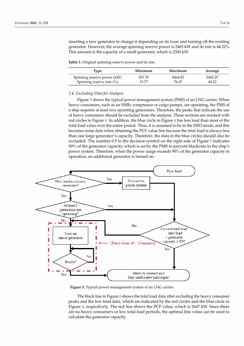
Figure 5 shows the typical power management system (PMS) of an LNG carrier. Whenheavy consumers, such as an SMRc compressor or cargo pumps, are operating, the PMS ofa ship requires at least two operating generators. Therefore, the peaks that indicate the useof heavy consumers should be excluded from the analysis. These sections are marked withred circles in Figure 4. In addition, the blue circle in Figure 4 has less load than most of thetotal load value over the entire period. Thus, it is assumed to be in the HFO mode, and thisbecomes noise data when obtaining the PCF value line because the total load is always lessthan one large generator’s capacity. Therefore, the data in the blue circles should also beexcluded. The number 0.9 in the decision symbol on the right side of Figure 5 indicates90% of the generator capacity, which is set by the PMS to prevent blackouts in the ship’spower system. Therefore, when the power usage exceeds 90% of the generator capacity inoperation, an additional generator is turned on.

Figure 5. Typical power management system of an LNG carrier.

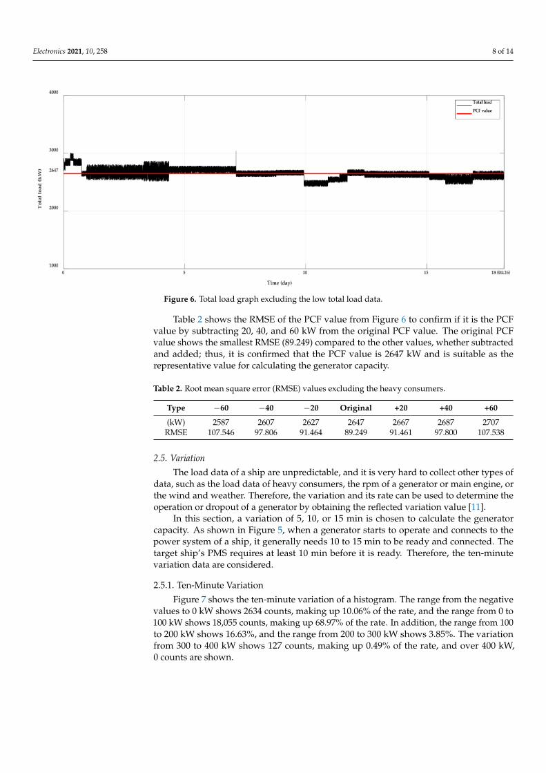
The black line in Figure 6 shows the total load data after excluding the heavy consumerpeaks and the low total data, which are indicated by the red circles and the blue circle inFigure 4, respectively. The red line shows the PCF value, which is 2647 kW. Since thereare no heavy consumers or low total load periods, the optimal line value can be used tocalculate the generator capacity.

Electronics 2021, 10, 258 8 of 14

Figure 6. Total load graph excluding the low total load data.

Table 2 shows the RMSE of the PCF value from Figure 6 to confirm if it is the PCFvalue by subtracting 20, 40, and 60 kW from the original PCF value. The original PCFvalue shows the smallest RMSE (89.249) compared to the other values, whether subtractedand added; thus, it is confirmed that the PCF value is 2647 kW and is suitable as therepresentative value for calculating the generator capacity.

Table 2. Root mean square error (RMSE) values excluding the heavy consumers.

Type −60 −40 −20 Original +20 +40 +60

(kW) 2587 2607 2627 2647 2667 2687 2707RMSE 107.546 97.806 91.464 89.249 91.461 97.800 107.538

2.5. Variation

The load data of a ship are unpredictable, and it is very hard to collect other types ofdata, such as the load data of heavy consumers, the rpm of a generator or main engine, orthe wind and weather. Therefore, the variation and its rate can be used to determine theoperation or dropout of a generator by obtaining the reflected variation value [11].

In this section, a variation of 5, 10, or 15 min is chosen to calculate the generatorcapacity. As shown in Figure 5, when a generator starts to operate and connects to thepower system of a ship, it generally needs 10 to 15 min to be ready and connected. Thetarget ship’s PMS requires at least 10 min before it is ready. Therefore, the ten-minutevariation data are considered.

2.5.1. Ten-Minute Variation

Figure 7 shows the ten-minute variation of a histogram. The range from the negativevalues to 0 kW shows 2634 counts, making up 10.06% of the rate, and the range from 0 to100 kW shows 18,055 counts, making up 68.97% of the rate. In addition, the range from 100to 200 kW shows 16.63%, and the range from 200 to 300 kW shows 3.85%. The variationfrom 300 to 400 kW shows 127 counts, making up 0.49% of the rate, and over 400 kW,0 counts are shown.

Electronics 2021, 10, 258 9 of 14

Figure 7. Ten-minute variation histogram.

2.5.2. Overall Variation

Table 3 shows 1, 5, 10, and 15 min of variation and the rates thereof. All variationsafter the 400 kW range show 0 counts. Therefore, the reflected variation value is up to400 kW when calculating the capacity of the generator.

Table 3. Results of the 1, 5, 10, and 15 min variation.

Range (kW)1 min 5 min 10 min 15 min

Count Rate (%) Count Rate (%) Count Rate (%) Count Rate (%)

(−999)–0 13,214 50.46 5301 20.25 2634 10.06 1731 6.611–99 11,300 43.15 16,913 64.60 18,055 68.97 18,307 69.95

100–199 1407 5.37 3211 12.26 4354 16.63 4812 18.39200–299 243 0.93 679 2.59 1007 3.85 1149 4.39300–399 21 0.08 78 0.30 127 0.49 173 0.66400–499 0 0.00 0 0.00 0 0.00 0 0.00500–599 0 0.00 0 0.00 0 0.00 0 0.00600–699 0 0.00 0 0.00 0 0.00 0 0.00700–799 0 0.00 0 0.00 0 0.00 0 0.00800–899 0 0.00 0 0.00 0 0.00 0 0.00900–999 0 0.00 0 0.00 0 0.00 0 0.00

The PCF value from Section 2.4 is 2647 kW, and the highest reflected variation valuefrom Table 3 is 400 kW. To choose the representative value, the PCF value and reflectedvariation value should be added, which amounts to 3047 kW.

3. Case Studies and Results

The PCF value from Section 2.4 is 2647 kW, and the highest reflected variation value is400 kW. Therefore, the representative capacity of the generator is 3047 kW, which is shownwith the red-colored line in Figure 8. Figure 8 also shows the possible generator selection.The green-colored line is for a 3680 kW generator that has a total of eight cylinders. Themagenta-colored line is a 3220 kW generator that has a total of seven cylinders. The blue-colored line is a 2760 kW generator that has a total of six cylinders. If a generator’s capacityis less than 2760 kW, at least two generators will always be needed to operate. Therefore,2760 kW is the minimum selection for the large generator.

Electronics 2021, 10, 258 10 of 14

Figure 8. Each generator’s capacity.

The values to be considered in calculating the total capacity are the number of genera-tors and the capacity of each generator. In Section 2.3, the highest load was shown to be8327 kW, which means that the reserve power is 2713 kW. Therefore, if the total capacity ofthe generator is higher than 8327 kW, then it is safe for any situation. Furthermore, 2713 kWindicates the total generator capacity. This is larger than the small generator capacity whichis 2300 kW. Therefore, the number of generators can be operated with three units instead ofthe existing four units. Otherwise, each of the four generators can reduce the units of thecylinder. However, it is more advantageous to reduce the number of generator units from4 to 3 rather than reducing the number of cylinders for four generators in securing spacein the ship’s machine room. However, for securing space in the ship’s machine room, itis more advantageous to reduce the number of generator units rather than reducing thenumber of cylinders.

Therefore, in the case studies, each of the generator capacities was selected accordingto the numbers of cylinders that would be considered in reality. In addition, a total of threegenerator combinations were denoted as Cases 1–3, and they are listed in Table 4. Theresults of each case study are compared with the spinning reserve power of the originalcase and those of Cases 1–3. The reasoning behind comparing the spinning reserve poweris to see the efficiency of each case. The safeness of each case is also compared to see if theresults can be considered from a practical perspective.

Table 4. Generator combinations for each case.

Case 1 2760 kW 1840 kW Total

Number of generators 2 2 4Total power of generators 5520 kW 3680 kW 9200 kW

Case 2 3220 kW 2300 kW Total

Number of generators 2 1 3Total power of generators 6440 kW 2300 kW 8740 kW

Case 3 3680 kW 2300 kW Total

Number of generators 2 1 3Total power of generators 7360 kW 2300 kW 9660 kW

3.1. Case 1

The combination of generators in Case 1 involves a total of three generators. Theselected generator capacities are two 2760 kW generators and two 1840 kW generators. Thereduction in the cylinders of the original small generator is because of the total capacity.

Electronics 2021, 10, 258 11 of 14

If this combination would have two 2300 kW generators instead of 1840 kW generators,then the total capacity would be 10,120 kW. This is larger than the original total capacity. Inaddition, if one of the 2300 kW generators was reduced, then the total capacity would be7820 kW, which is smaller than the highest load. According to Figure 4, from the beginningto around day 7, the PMS requires at least two generators because the load values are over2760 kW, which will cause large amounts of reserve power to be generated.

The blue-colored line in Figure 9 shows the spinning reserve power for Case 1. Theblue line is compared with the original spinning reserve power. The spinning reservepower of Case 1 comes close to the total load data, which means that the spinning reservepower is reduced. However, from around day 7 to around day 14, the spinning reservepower shows a much higher total load than on other days. This is because the total loadexceeds the capacity of a large generator, so another generator turns on to make up forthe difference.

Figure 9. Spinning reserve power of all cases and original case.

3.2. Case 2

The combination of generators in Case 2 comprises a total of three generators. Theselected generator capacities are two 3220 kW generators and a 2300 kW generator. Thiscombination can handle the highest load because the total capacity is 8740 kW, which is 413kW larger than the maximum; as shown in Figure 9, all of the load data are under 3220 kW,which is reliable.

The magenta-colored line in Figure 9 shows the spinning reserve power for Case 2.Compared with the original spinning reserve power, the spinning reserve power of Case 2comes closer to the total load data. In addition, compared with the results of Case 1, thepeak of the magenta-colored line rises only when necessary. Moreover, the total capacityof the generator is less than in Case 1. Therefore, the highest peak at around day 14 iscloser to the total than that of Case 1. Each capacity of the generator is larger than in Case 1.However, the peak of Case 2 from around day 7 to day 14 is less than that of Case 1. This isbecause the large generator in Case 2 has enough capacity for that period’s total load.

3.3. Case 3

The combination of generators in Case 3 comprises a total of three generators. Theselected generator capacities were two 3680 kW generators and a 2300 kW generator. Thiscombination can handle the greatest load because the total capacity is 9660 kW, which is1333 kW greater than the maximum load. According to Figure 8, all of the load data areunder 3680 kW, which is reliable.

Electronics 2021, 10, 258 12 of 14

The green-colored line in Figure 9 shows the spinning reserve power for Case 3.Compared with the original spinning reserve power, most of the spinning reserve powerof Case 3 comes closer to the total load data. The reason that some periods have a higherspinning reserve power than the original spinning reserve power is that the large generatorin Case 3 has a larger capacity than the original large generator. Therefore, in the situationof the operation of one generator, Case 3 shows a higher spinning reserve power than theoriginal spinning reserve power. Compared with the results of Cases 1 and 2, there arefewer rising peaks of the green-colored line than for the previous cases. Around day 1 andright after day 5, the peaks in the low total load period are lower than the large capacity ofthe generator. Therefore, no more than one large generator is needed. Moreover, since theperiod needs only one generator, the spinning reserve power of Case 3 is higher than thatof Cases 1 and 2.

3.4. Results

Table 5 shows the overall spinning reserve power and the rates of the original caseand Cases 1–3. The lowest result for the minimum spinning reserve power is that of Case 2,which is 504.23 kW lower than the original minimum spinning reserve power. The lowestresult for the maximum spinning reserve power is that of Case 1, which is 5839.86 kWlower than the original maximum spinning reserve power. The lowest average result forthe spinning reserve power is that of Case 1, which is 1631.69 kW lower than the averageof the original spinning reserve power.

Table 5. Overall results for the spinning reserve power and rate.

Original Case 1

Minimum Maximum Average Minimum Maximum Average

Spinning reservepower (kW) 507.70 8464.82 2465.27 6.70 2624.96 833.58

Spinning reserve rate (%) 15.77 76.67 44.22 0.10 57.06 20.57

Case 2 Case 3

Minimum Maximum Average Minimum Maximum Average

Spinning reservepower (kW) 3.47 2864.74 893.82 13.40 3399.86 1295.11

Spinning reserve rate (%) 0.10 51.90 23.39 0.22 56.85 31.30

Table 6 shows the practical safeness of each case. The first row shows the results whenthe capacity of the large generator is close to the PCF value. This is important becausethe efficiency decreases as the capacity of the generator moves away from the PCF valueline, which represents the optimal efficiency. Case 2 shows the closest capacity of thegenerator, and Case 3 shows the farthest capacity of the generator. The second row showshow frequently each case exceeds the capacity of the large generator over the entire timeperiod, which includes the red and blue circle periods in Figure 4. This frequency cancause a ship to be threatened with blackouts, so it is advantageous to have as few casesas possible in order to be on the stable side. However, this must be considered carefullybecause a lower chance of exceeding the capacity means a lower efficiency. The worst caseis Case 1, in which the capacity is exceeded 1332 times. This means that there are manytimes when another generator needs to be turned on for just a little more electricity. Cases2 and 3 show a frequency of 0, so Cases 2 and 3 have the same safeness.

Electronics 2021, 10, 258 13 of 14

Table 6. Checklist for practical consideration.

Case 1 Case 2 Case 3

Is the large generator’s capacityclose to the PCF value?

(difference from the PCF value)

A little far(−287 kW)

Close(+173 kW)

Far(+633 kW)

Frequency of exceedingthe large generator’s capacity

(safety index)1331 0 0

Overall, Cases 1 to 3 show better results for the spinning reserve power and its ratethan the original data. The best choice for safety is either Case 2 or Case 3, both of whichhave 0 total loads that exceed the capacity of the large generator. The most efficient choiceis Case 1, which has the lowest average reserve power. However, in Case 1, the total loadis very close to the capacity of the generator for a long time, so there is a high safety risk.Case 3 shows the farthest value from the PCF value, which means that Case 2 is a betterchoice than Case 3. Moreover, Case 2 is closest to the PCF value, which means that it isthe best in terms of efficiency and safety. The safeness of Case 2 and the original data aresimilar because they use the same generator capacity for the large generator. However,the efficiency of Case 2 is much better than that of the original data, as seen in Table 5. Asseen in Table 7, the GCSI value of Case 2 is 23.39, which is the minimum value in all cases.Therefore, Case 2 has the optimal generator capacity. It operates with a total of three unitsof generators by removing a 2300 kW generator from the four original generator units.

Table 7. Generator capacity selection index (GCSI) value of each case.

Original Case Case 1 Case 2 Case 3

GCSI Value 57.75 33.88 23.39 31.3

4. Conclusions

In this paper, the total load data were analyzed by excluding interfering data. Withthe total load data analyzed, the PCF value was obtained through PCF. After that, thePCF value was added to the most suitable reflected variation value, which was obtainedthrough variation analysis. Case studies were practically applied; the capacity of a cylinderwas set to 460 kW and the generators’ capacities were selected and composed accordingly.In addition, the case studies were analyzed and compared with the original case usingthe GCSI method to figure out which case’s generator combination had the most optimalgenerator capacity. According to GCSI results, it was concluded that Case 2 was themost suitable in terms of safety and efficiency; it was possible to replace the four existinggenerators with three units of generators in Case 2. Therefore, if Case 2 is applied, space canbe secured in the machine room, so more equipment can be installed—such as for reducingSOx emissions—and more cargo can be loaded. Furthermore, the energy efficiency can alsobe increased by applying a lower reserve ratio than that of the original case to cover thehighest total load.

Author Contributions: This research was conducted with the collaboration of all authors. J.L., wrotethe paper; J.-W.P. and H.-J.L., supervised the paper. All authors have read and agreed to the publishedversion of the manuscript.

Funding: This work was supported in part by the Basic Science Research Program through theNational Research Foundation of Korea (NRF) funded by the Ministry of Education (Grant number:2016R1D1A3B03934501) and in part by the National Research Foundation of Korea (NRF) (Grantnumber: 2020R1A3B2079407), the Ministry of Science and ICT (MIST), Korea.

Conflicts of Interest: The authors declare no conflict of interest.

Electronics 2021, 10, 258 14 of 14

References1. Corbett, J.J.; Winebrake, J.J.; Carr, E.W.; Jalkanen, J.-P.; Johansson, L.; Prank, M.; Sofiev, M. Health Impacts Associated with Delay

of MARPOL Global Sulphur Standard. Mar. Environ. Prot. 2016, 15, 6–19.2. Hein, K.; Yan, X.; Wilson, G. Multi-Objective Optimal Scheduling of a Hybrid Ferry with Shore-to-Ship Power Supply Considering

Energy Storage Degradation. Electronics 2020, 9, 849. [CrossRef]3. Chen, L.; Tong, Y.; Dong, Z. Li-Ion Battery Performance Degradation Modeling for the Optimal Design and Energy Management

of Electrified Propulsion Systems. Energies 2020, 13, 1629. [CrossRef]4. Dvornik, J. Dual-Fuel-Electric Propulsion Machinery Concept on LNG Carriers. Trans. Marit. Sci. 2014, 12, 137–148. [CrossRef]5. Rehman, A.; Qyyum, M.A.; Zakir, F.; Nawaz, S.; He, X.; Razzaq, L.; Lee, M.; Wang, L. Investigation of improvement potential

of Modified Single Mixed Refrigerant (MSMR) LNG process in terms of avoidable and unavoidable exergy destruction. InProceedings of the 2020 3rd International Conference on Computing, Mathematics and Engineering Technologies (iCoMET),Sukkur, Pakistan, 29–30 January 2020; pp. 1–7.

6. Lassesson, H.; Andersson, K. Energy Efficiency in Shipping; Department of Shipping and Marine Technology, Division of SustainableShip Propulsion, Charmers University of Technology: Göteborg, Sweden, 2009; Volume 6, pp. 12–17.

7. Godjevac, M.; Mestemaker, B.T.W.; Visser, K.; Lyu, Z.; Boonen, E.J.; van der Veen, F.; Malikouti, C. Electrical energy storage fordynamic positiong operations: Investigation of three application case. In Proceedings of the IEEE Electric Ship TechnologiesSymposium, ESTS, Arlington, VA, USA, 14–17 August 2017; Volume 5, pp. 182–186.

8. Huan, T.; Hongjun, F.; Wei, L.; Guoquang, Z. Options and Evaluations on Propulsion Systems of LNG Carriers. In PropulsionSystems; IntechOpen: London, UK, 2019; pp. 1–20.

9. Numaguchi, H.; Satoh, T.; Ishida, T.; Matsumoto, S.; Hino, K.; Iwasaki, T. Japan’s First Dual-Fuel Diesel-Electric PropulsionLiquefied Natural Gas (LNG) Carrier. Mitsubishi Heavy Ind. Tech. Rev. 2009, 4, 1–4.

10. Yang, R.; Yuan, Y.; Ying, R.; Shen, B.; Long, T. A Novel Energy Management Strategy for a Ship’s Hybrid Solar Energy GenerationSystem Using a Particle Swarm Optimization Algorithm. Energies 2020, 13, 1380. [CrossRef]

11. Kim, Y.H.; Kim, S.H. Variations of wind power generation in Korea-Jeju power system. In Proceedings of the IEEE/PESTransmission and Distribution Conference and Exhibition: Asia and Pacific, Seoul, Korea, 26–30 October 2009; Volume 4, pp. 1–4.