
A Study of Alternative Gas Mixtures of RPC & Different Aspects ...
225
A Study of Alternative Gas Mixtures of RPC & Different Aspects of Neutrino Oscillation for ICAL at INO By JAYDEEP DATTA PHYS01201504022 Bhabha Atomic Research Center A thesis submitted to the Board of Studies in Physical Sciences In partial fulfillment of requirements for the Degree of DOCTOR OF PHILOSOPHY of HOMI BHABHA NATIONAL INSTITUTE April 2021
-
Upload
khangminh22 -
Category
Documents
-
view
3 -
download
0
Transcript of A Study of Alternative Gas Mixtures of RPC & Different Aspects ...
A Study ofAlternative Gas Mixtures of RPC
&Different Aspects of Neutrino Oscillation
for ICAL at INO
By
JAYDEEP DATTA
PHYS01201504022
Bhabha Atomic Research Center
A thesis submitted to theBoard of Studies in Physical Sciences
In partial fulfillment of requirementsfor the Degree of
DOCTOR OF PHILOSOPHYof
HOMI BHABHA NATIONAL INSTITUTE
April 2021


Homi Bhabha National Institute
Recommendations of the Viva Voce Committee
As members of the Viva Voce Committee, we certify that we have read the
dissertation prepared by Jaydeep Datta entitled “A Study of Alternative Gas
Mixtures of RPC & Different Aspects of Neutrino Oscillation for ICAL at
INO” and recommend that it may be accepted as fulfilling the thesis requirement
for the award of Degree of Doctor of Philosophy.
Final approval and acceptance of this thesis is contingent upon the
candidate’s submission of the final copies of the thesis to HBNI.
We hereby certify that we have read this thesis prepared under our direction
and recommend that it may be accepted as fulfilling the thesis requirement.
Date: July 28, 2021
Place: SINP, Kolkata Prof. S. Umasankar (Coguide) Prof. N. Majumdar (Guide)
Chairman - Prof. Supratik Mukhopadhyay Date:
Guide / Convener - Prof. Nayana Majumdar Date:
Co-guide / Co-convener - Prof. Sankagiri Umasankar Date:
Examiner - Prof. James Libby Date:
Member 1 - Prof. Amol Dighe Date:
Member 2 - Prof. Gobinda Majumder Date:
Member 3 - Dr. Satyanarayan Bheesette Date:
28/7/2021
28/07/2021
28/07/2021
28
28/07/2021
28/07/2021
28/07/2021

Statement by the Author
This dissertation has been submitted in partial fulfillment of requirements for an
advanced degree at Homi Bhabha National Institute (HBNI) and is deposited in
the library to be made available to borrowers under rules of the HBNI.
Brief quotations from this dissertation are allowable without special permis-
sion, provided that accurate acknowledgement of source is made. Requests for
permission for extended quotation from or reproduction of this manuscript in
whole or in part may be granted by the Competent Authority of HBNI when
in his or her judgment the proposed use of the material is in the interests of
scholarship. In all other instances, however, permission must be obtained from
the author.
July 28, 2021
Kolkata
Jaydeep Datta


Declaration
I hereby declare that the investigation presented in the thesis has been carried out
by me. The work is original and has not been submitted earlier as a whole or in
part for a degree/diploma at this or any other Institution/University.
July 28, 2021
Kolkata
Jaydeep Datta

List of Publications Arising from
the Thesis
Publications in Refereed Journal
Published
1. Matter vs Vacuum Oscillation in Atmospheric Neutrinos, J. Datta, M.
Nizam, A. Ajmi and S. Umasankar, Nuclear Physics B, 961, 11521 (2020).
2. Study of Streamer development in Resistive Plate Chamber, J. Datta, S.
Tripathy, N. Majumdar and S. Mukhopadhyay, Journal of Instrumentation,
15, C12006 (2020).
3. Numerical Qualification of Eco-Friendly Gas Mixtures for Avalanche-
Mode Operation of Resistive Plate Chambers in INO-ICAL, J. Datta, S.
Tripathy, N. Majumdar and S. Mukhopadhyay, Journal of Instrumentation,
16, P07012 (2021).
Under Preparation
1. Determination of Neutrino Oscillation Parameters Using Track and Non-
Track Hit Information from GEANT4, J.Datta, B.Singh and S. Umasankar
Symposium and Conference Proceedings
1. Qualification of Eco-Friendly Gas Mixture for Avalanche Mode Operation
of RPC, J. Datta, A. Jash, N. Majumdar, S. Mukhopadhyay, “Advanced
Detectors for Nuclear, High Energy and Astroparticle Physics”, Chapter
12, Springer Proceedings, 2018.
Conferences
Oral Presentation
1. Qualification of Eco-friendly Gas Mixture for Avalanche Mode Opera-
tion of RPC, Advanced Detectors in Nuclear, High Energy, Astroparticle
Physics ADNHEAP 2017, February 15-17, 2017, Bose Institute, Kolkata,
India.
2. Modelling of Avalanches and Streamers in Resistive Plate Chambers, Inter-
national Conference onMathematicalModelling and Scientific Computing
ICMMSC 2018, July 19-21, 2018, Indian Institute of Technology, Indore,
India.
3. Study of Streamer Development in Resistive Plate Chamber, XVWorkshop
on Resistive Plate Chambers and Related Detectors, RPC 2020, February
10-14, 2020, University of Rome, Tor Vergata, Italy (Awarded the best oral
presentation).
4. Matter vs VacuumOscillation in Atmospheric Neutrinos, 40th International
Conference on High Energy Physics, ICHEP 2020, July 28 - August 6,
2020, Online Conference, Prague
Poster Presentation
1. Matter vs. Vacuum Oscillations Atmospheric Neutrinos, XXIX Interna-
tional Conference on Neutrino Physics and Astrophysics, Neutrino 2020,
Online conference, Chicago (USA), June 22 - July 2 (2020).
2. Neutrino oscillation parameter determination at INO-ICAL using track
and non-track hit information from GEANT, XIV DAE-BRNS High En-
ergy Physics Symposium, DAE-HEP, Online Conference, Bhubaneswar
(India), December 14 – December 18 (2020)
July 28, 2021
Kolkata
Jaydeep Datta


Dedicated to
My Family


Acknowledgements
Throughout my doctoral study, many people have contributed and supported me,
directly or indirectly. I would like to use this space to express my gratitude to
all of them. First and foremost, I want to thank my supervisor Prof. Nayana
Majumdar and co-supervisor Prof. Sankagiri Umasankar for giving me such
beautiful and interesting problems to work on. Throughout my doctoral study
they have supported, motivated and guided me towards successful completion
of the projects. In this five year long beautiful journey members of my doctoral
committee, Prof. Supratik Mukhopadhyay, Prof. Amol Dighe, Prof. Gobinda
Majumder, Dr. Satyanarayana Bheesette and Prof. Satyajit Saha guided me with
their experience and knowledge. I like to thank them all.
I would like to thank my father, Jitendra Narayan Datta, mother, Juin Datta
and sister, Jayeeta Datta, who always supported my dream and encouraged me to
go for it. In this five year long journey, many ups and downs have come along the
path. They have supported me through these ups and downs. In this five year I
have been stationed at many institutes all around India due to my mixed nature of
work. I roamed around here and there and made many friends who supported me
when I needed them. My friends from TIFR, Sabir, Subhajit, Uttiya, Anustup,
Sounak, Argha, Soumen andAnupam always cheeredme upwhen I felt low. Late
night discussions with them on every possible topics enriched and energized me
for the next day. My friends at SINP, Sridhar, Prashant, Arpita, Dr. Bankim da,
Sayan and Shubham helped me throughout my Ph.D. tenure. A tea with them
chargedme up whenever I felt tired. Along with them, my school friend Ritabrata
was always there to share experiences. I will also like to thankmy juniors, Vishal,
Promita, Ram, Anil, Tanay, Pralay, Subhendu, Subharaj, Maudud, Mamta, Jim,
Sadashiv for their support.
I would like to thank the INO family for taking me in and helping me to
grow. I feel blessed to have seniors like Dr. Varchaswi Kashyap, Dr. Neha
Panchal, Dr. Abhijit Garai, Dr. Apoorva Bhatt, Dr. Md. Nizam, Dr. Harishree
Krishnamoorthy, Dr. S. Pethuraj, Dr. Chandan Gupta, Dr. Abhik Jash, Dr.
Ali Ajmi, Dr. Amina Khatun, Dr. Deepak Tiwari, Dr. Suryanarayan Mondal
and Dr. Moon Moon Devi for helping and guiding me whenever needed. My
INO batchmates Dr. Dhruv Mulmule and Dr. Aparajita Majumdar made my
stay at Wadala enjoyable. My experimental works wouldn’t have been successful
without helps fromMandar ji, Yuvraj, Pataleshwar, Dipankar da, Shinde ji, Visal
ji, Ganesh ji, Pradipta da, Chandranatrh da and Saibal da. Whenever I needed
any support regarding my computational works, Nagaraj sir, Pawan ji and SINP
computer division helped me a lot.
I would like to thank DHEP of TIFR and ANP Divison of SINP for their
support. Thanks, to all of you, for this pleasant and memorable journey.
Summary
Iron Calorimeter (ICAL) is a 50 kt magnetized calorimeter to be housed at
the underground facility of India-based Neutrino Observatory (INO) to study
atmospheric neutrinos. The detector will be populated with a stack of Resistive
Plate Chambers (RPCs) alternated with iron slabs, which will play the role of
fixed target for the atmospheric neutrinos. The charged leptons generated in the
interaction of the neutrino and the iron nuclei will be tracked by the RPCs during
their flight through the ICAL along a curved path due to a high magnetic field
applied across the ICAL. The tracking information will be utilized to study the
properties of the parent neutrinos. This doctoral thesis addresses a few aspects
related to both of the detector development and phenomenological studies related
to the ICAL. The work in connection to the detector development has been
carried out to search for alternative eco-friendly gas mixtures for avalanche
mode operation of the RPCs. On the other hand, the sensitivity study of the
ICAL to earth matter effect and development of an analysis method to improve
the precision of oscillation parameter measurement have been performed as
i
ii
phenomenological research work.
The physics goals of ICAL experiment demands avalanche mode operation of
the RPCs to meet the appropriate spatial and time resolution required for neutrino
flux measurement. The standard mixture of tetrafluoroethane (R134a), isobutane
(i-C4H10) and sulfur hexafluoride (SF6) used to operate RPCs in avalanche mode
has negative impact on the environment due to its high GlobalWarming Potential
(GWP) (∼ 1430). This calls for replacement of this mixture with a suitable one
to achieve the experiment goals without affecting the nature. In this context,
a numerical simulation framework has been developed to simulate efficiency
and streamer probability of RPC from the basic properties of any gas mixture.
The validation of this simulation framework has been done by comparing the
simulated results for different gas mixtures with experimental data available for
them. In all the scenarios, the simulated data have closely followed the ex-
periment validating the simulation framework. Once validated, the simulation
framework has been used to simulate an argon, carbon dioxide and nitrogen based
gas mixture which is eco-friendly (GWP < 1), non-flammable and economically
cheap. It has been observed that without inclusion of SF6 the proposed mixture
is not as suitable as the standard mixture in terms of streamer probability but has
shown similar performance to different eco-friendly gas mixtures proposed by
other experiments. Inclusion of SF6 has been found to improve its performance
marginally, whereas reduction of signal threshold has demonstrated greater im-
pact on its performance. In case of reduced threshold, the Ar-based gas mixture
performs similar to the standard R134a-based gas mixture and sometimes better
than the other eco-friendly gas mixtures proposed by other experiments. An
added advantage of the proposed Ar-based gas mixture is its operation at com-
iii
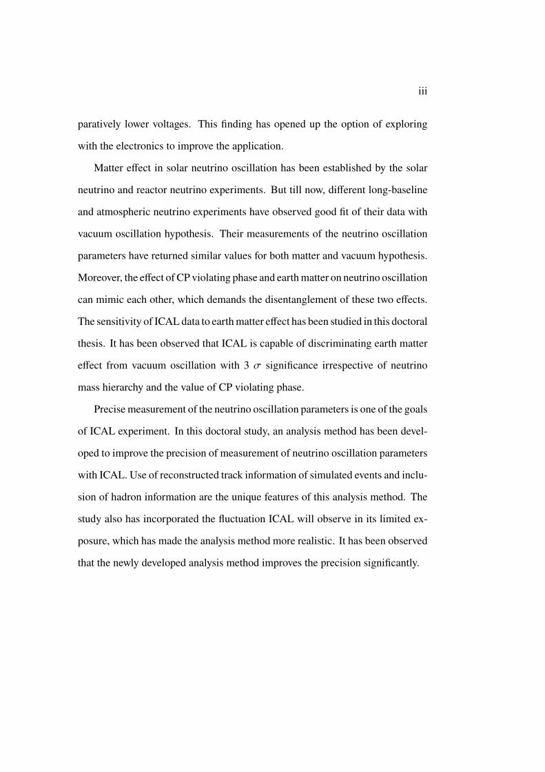
paratively lower voltages. This finding has opened up the option of exploring
with the electronics to improve the application.
Matter effect in solar neutrino oscillation has been established by the solar
neutrino and reactor neutrino experiments. But till now, different long-baseline
and atmospheric neutrino experiments have observed good fit of their data with
vacuum oscillation hypothesis. Their measurements of the neutrino oscillation
parameters have returned similar values for both matter and vacuum hypothesis.
Moreover, the effect of CP violating phase and earthmatter on neutrino oscillation
can mimic each other, which demands the disentanglement of these two effects.
The sensitivity of ICALdata to earthmatter effect has been studied in this doctoral
thesis. It has been observed that ICAL is capable of discriminating earth matter
effect from vacuum oscillation with 3 f significance irrespective of neutrino
mass hierarchy and the value of CP violating phase.
Precise measurement of the neutrino oscillation parameters is one of the goals
of ICAL experiment. In this doctoral study, an analysis method has been devel-
oped to improve the precision of measurement of neutrino oscillation parameters
with ICAL. Use of reconstructed track information of simulated events and inclu-
sion of hadron information are the unique features of this analysis method. The
study also has incorporated the fluctuation ICAL will observe in its limited ex-
posure, which has made the analysis method more realistic. It has been observed
that the newly developed analysis method improves the precision significantly.

iv
Contents
Summary i
List of Figures xi
List of Tables xvii
List of Abbreviations xix
1 Introduction 1
2 Iron Calorimeter Detector 13
2.1 Iron Calorimeter . . . . . . . . . . . . . . . . . . . . . . . . . . 14
2.2 Magnet of ICAL . . . . . . . . . . . . . . . . . . . . . . . . . . 18
2.3 Readout system . . . . . . . . . . . . . . . . . . . . . . . . . . 20
3 Simulation Framework of ICAL 23
3.1 Event Generation . . . . . . . . . . . . . . . . . . . . . . . . . 24
3.2 Event Simulation and Digitization . . . . . . . . . . . . . . . . 26
v
vi CONTENTS
3.3 Event Reconstruction . . . . . . . . . . . . . . . . . . . . . . . 27
3.3.1 Track finding . . . . . . . . . . . . . . . . . . . . . . . 27
3.3.2 Track fitting . . . . . . . . . . . . . . . . . . . . . . . . 29
3.4 Analysis Method . . . . . . . . . . . . . . . . . . . . . . . . . 31
3.4.1 Oscillation Probability Calculator . . . . . . . . . . . . 31
I Study of alternative gas mixtures of RPC for ICAL at
INO 33
4 Resistive Plate Chamber 35
4.1 Construction . . . . . . . . . . . . . . . . . . . . . . . . . . . . 36
4.2 Working Principle . . . . . . . . . . . . . . . . . . . . . . . . . 38
4.2.1 Avalanche Mode . . . . . . . . . . . . . . . . . . . . . 39
4.2.2 Streamer mode . . . . . . . . . . . . . . . . . . . . . . 41
4.2.2.1 Positive Streamer or Cathode Directed Streamer 42
4.2.2.2 Negative Streamer or Anode Directed Streamer 43
5 Numerical Modelling of RPC 45
5.1 Numerical Modelling . . . . . . . . . . . . . . . . . . . . . . . 46
5.1.1 Model Geometry . . . . . . . . . . . . . . . . . . . . . 47
5.1.2 Mathematical Model . . . . . . . . . . . . . . . . . . . 48
5.1.3 Conditions for Avalanche and Streamer . . . . . . . . . 51
5.2 Simulated Avalanche and Streamer Discharge . . . . . . . . . . 52
5.3 Calculation of Streamer Probability and Efficiency . . . . . . . . 55
5.3.1 Event Generation . . . . . . . . . . . . . . . . . . . . . 56
5.3.2 Estimation of Detector Responses . . . . . . . . . . . . 59
CONTENTS vii
5.4 Validation of Numerical Model . . . . . . . . . . . . . . . . . . 61
5.4.1 Comparison for R134a(95%):n-C4H10(5%) . . . . . . . 62
5.4.2 Comparison for R134a(95.2%):i-C4H10 (4.5%):SF6(0.3%) 64
6 Experimental Studies 67
6.1 RPC Fabrication . . . . . . . . . . . . . . . . . . . . . . . . . . 68
6.2 Experimental Setup and Data Acquisition . . . . . . . . . . . . 71
6.3 Analysis Method . . . . . . . . . . . . . . . . . . . . . . . . . 74
6.4 Results . . . . . . . . . . . . . . . . . . . . . . . . . . . . . . . 76
7 Numerical Qualification of Eco-Friendly Gas Mixture 83
7.1 Choice of Gas Mixture . . . . . . . . . . . . . . . . . . . . . . 84
7.2 Qualification of Ar(5%):CO2(60%):N2(35%) . . . . . . . . . . 87
7.2.1 Comparison with R134a-based Mixture . . . . . . . . . 88
7.2.2 Comparison with HFO1234ze-based Mixtures . . . . . . 91
II Study of different aspects of neutrino oscillation for
ICAL at INO 97
8 Neutrino Oscillations in Vacuum and in Matter 99
8.1 Neutrino oscillation in vacuum . . . . . . . . . . . . . . . . . . 100
8.1.1 Two Flavor Oscillation . . . . . . . . . . . . . . . . . . 100
8.1.2 Three Flavor Oscillation . . . . . . . . . . . . . . . . . 102
8.2 Neutrino oscillation in matter . . . . . . . . . . . . . . . . . . . 104
8.2.1 Effective matter potential . . . . . . . . . . . . . . . . . 105
8.2.2 Two flavor neutrino oscillation in matter . . . . . . . . . 106
viii CONTENTS
8.2.3 Three flavor neutrino oscillation in matter . . . . . . . . 108
9 Matter vs Vacuum Oscillation in Atmospheric Neutrinos 113
9.1 Vacuum vs. Matter Modified Oscillations . . . . . . . . . . . . 117
9.2 Methodology . . . . . . . . . . . . . . . . . . . . . . . . . . . 119
9.3 Results . . . . . . . . . . . . . . . . . . . . . . . . . . . . . . . 122
10 Neutrino Oscillation Parameter Determination Using GEANT4
Reconstructed Event Information 135
10.1 Methodology . . . . . . . . . . . . . . . . . . . . . . . . . . . 136
10.1.1 Data and Theory sample . . . . . . . . . . . . . . . . . 136
10.1.2 Variables for Analysis . . . . . . . . . . . . . . . . . . . 138
10.1.3 Analysis Methods . . . . . . . . . . . . . . . . . . . . . 139
10.1.4 Systematic Errors and j2Calculation . . . . . . . . . . . 141
10.2 Results . . . . . . . . . . . . . . . . . . . . . . . . . . . . . . . 143
10.2.1 Procedure to Calculate Best fit point, 2 f and 3 f range . 143
10.2.2 Results for 5 and 10 year exposure time . . . . . . . . . 144
10.3 Conclusion . . . . . . . . . . . . . . . . . . . . . . . . . . . . 144
11 Conclusion and Outlook 153
11.1 Exploration for alternative gas mixtures of the RPCs . . . . . . . 154
11.2 Discrimination of matter effect from vacuum oscillation in atmo-
spheric neutrino oscillation . . . . . . . . . . . . . . . . . . . . 157
11.3 Determination of neutrino oscillation parameters using track and
hit information from GEANT4 . . . . . . . . . . . . . . . . . . 158
A Appendix 161

CONTENTS ix
A.1 Calculation of systematic errors . . . . . . . . . . . . . . . . . . 161
Bibliography 165

x CONTENTS

List of Figures
1.1 A schematic representation of Standard Model [1]. . . . . . . . . . 2
1.2 Neutrino flux ratio as function of Ea calculated by Bartol group
[49], Fluka Group [50], HKKMS06 [51] and HKKM11 [52] for the
Kamioka site, Japan [48]. . . . . . . . . . . . . . . . . . . . . . . . 7
2.1 (a) INO site at Bodi West Hills [59], (b) Cosmic ray flux as function
of water equivalent depth [59]. . . . . . . . . . . . . . . . . . . . . 14
2.2 Schematic diagram of ICAL [59]. . . . . . . . . . . . . . . . . . . . 15
2.3 Schematic diagram of the closed loop gas mixing unit to be used at
ICAL [64]. . . . . . . . . . . . . . . . . . . . . . . . . . . . . . . . 17
2.4 (a) Schematic diagram of copper coil in each module of ICAL [65].
(b) Magnetic field map in the central plate of the central module (Z
= 0) the magnitude (in T) [59]. . . . . . . . . . . . . . . . . . . . . 20
2.5 Schematic diagram of data flow and storage of ICAL [67]. . . . . . 21
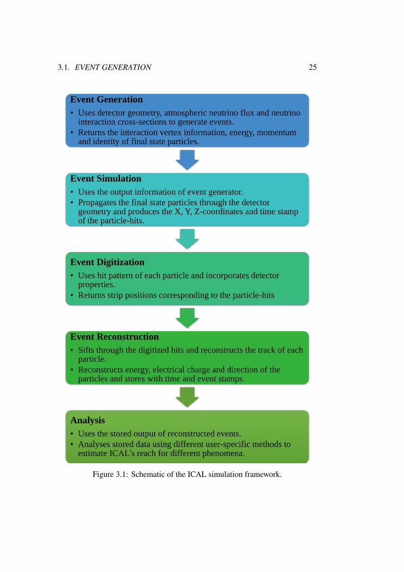
3.1 Schematic of the ICAL simulation framework. . . . . . . . . . . . . 25
3.2 An example of simulated a` CC interaction in the detector [81]. . . 28
xi
xii LIST OF FIGURES
4.1 Transverse cross-sectional view of RPC. . . . . . . . . . . . . . . . 37
4.2 Longitudinal cross-sectional view of RPC. . . . . . . . . . . . . . . 38
4.3 Growth of avalanche. The black-arrows depicts the field lines due to
the space charge. The blue arrows show the filed lines of the applied
electric field.[93] . . . . . . . . . . . . . . . . . . . . . . . . . . . 40
4.4 Schematic diagram of positive streamer formation [93]. . . . . . . . 42
4.5 Schematic diagram of negative streamer [93]. . . . . . . . . . . . . 43
5.1 Geometry of the model. . . . . . . . . . . . . . . . . . . . . . . . . 48
5.2 Growth of electronic charges in RPC for avalanche at 41 kV/cm for
10 primary electrons with mean Z-position of 1.2 mm . . . . . . . . 52
5.3 Growth of electronic charges in RPC for streamer at 47 kV/cm for 10
electrons with mean Z-position of 1.2 mm . . . . . . . . . . . . . . 53
5.4 Time evolution of electric field and electron density at applied field
47 kV/cm . . . . . . . . . . . . . . . . . . . . . . . . . . . . . . . 54
5.5 Induced current in case of a streamer event at 47 kV/cm . . . . . . . 55
5.6 Total number of electrons for the gasmixtureR134a (95%):n-C4H10(5%). 57
5.7 2D histogram of muon events for the gas mixture of R134a (95%):n-
C4H10 (5%). . . . . . . . . . . . . . . . . . . . . . . . . . . . . . . 59
5.8 2D histogram ofmuon events for the gasmixture of R134a (95.2%):i-
C4H10 (4.5%):SF6 (0.3%). . . . . . . . . . . . . . . . . . . . . . . 60
5.9 Efficiency as a function of applied voltage forR134a(95%):n-C4H10(5%). 63
5.10 Streamer probability as a function of applied voltage for R134a
(95%):n-C4H10 (5%). . . . . . . . . . . . . . . . . . . . . . . . . . 63
LIST OF FIGURES xiii
5.11 Streamer probability as function of efficiency for R134a (95%):n-
C4H10 (5%). . . . . . . . . . . . . . . . . . . . . . . . . . . . . . . 64
5.12 Comparison of efficiency as function of high-voltage between simu-
lation (this work) and experiments [106, 107] for the gas mixture of
R134a (95.2%):i-C4H10 (4.5%):SF6 (0.3%). . . . . . . . . . . . . . 65
5.13 Comparison of streamer probability as a function of efficiency be-
tween simulation (this work) and experiments [106, 107] for the gas
mixture of R134a (95.2%):i-C4H10(4.5%):SF6(0.3%). . . . . . . . . 66
6.1 Different stages of a glass RPC fabrication. . . . . . . . . . . . . . . 70
6.2 Experimental setup a) Side view, b) Front view. . . . . . . . . . . . 71
6.3 Electronics modules used for experiment. . . . . . . . . . . . . . . 72
6.4 Schematic of the HMC based pre-amplifier board [111]. . . . . . . . 73
6.5 Schematic diagram of the experimental setup. . . . . . . . . . . . . 74
6.6 RPC signal at 10 kV with baseline calculated using post-trigger
information, depicted in red. . . . . . . . . . . . . . . . . . . . . . 75
6.7 Efficiency of a glass RPC as function of high-voltage for the gas
mixture of R134a(95.2%):i-C4H10(4.5%):SF6(0.3%). . . . . . . . . 76
6.8 Distribution of arrival times for a) 9.2 kV, b) 9.3 kV. . . . . . . . . . 77
6.9 Time resolution as function of high-voltage. . . . . . . . . . . . . . 78
6.10 Charge integration procedure. . . . . . . . . . . . . . . . . . . . . . 78
6.11 Distribution of induced charge for a) 10 kV and b) 10.2 kV. . . . . . 79
6.12 Average induced charge as function of high-voltage. . . . . . . . . . 79
6.13 Comparison of efficiency between experiment and simulation as
function of high-voltage. . . . . . . . . . . . . . . . . . . . . . . . 80
xiv LIST OF FIGURES
6.14 Comparison of streamer probability between experiment and simu-
lation as function of high-voltage. . . . . . . . . . . . . . . . . . . 81
7.1 Comparison of effectiveTownsend coefficient as a function of applied
voltage of proposed Ar (5%):CO2 (60%):N2 (35%) and Ar (5%):CO2
(60%):N2 (34.5%):SF6 (0.5%) mixture to that of R134a (95.2%):i-
C4H10 (4.5%):SF6 (0.3%) as obtained from MAGBOLTZ [104]. . . 87
7.2 Comparison of drift velocity as a function of applied voltage of pro-
posed Ar (5%):CO2 (60%):N2 (35%) and Ar (5%):CO2 (60%):N2
(34.5%):SF6 (0.5%)mixture to that ofR134a (95.2%):i-C4H10 (4.5%):SF6
(0.3%) as obtained from MAGBOLTZ [104]. . . . . . . . . . . . . 88
7.3 Comparison of primary electron number of proposed Ar (5%):CO2
(60%):N2 (35%) and Ar (5%):CO2 (60%):N2 (34.5%):SF6 (0.5%)
mixture to that of R134a (95.2%):i-C4H10 (4.5%):SF6 (0.3%) as ob-
tained from HEED [103]. The values have been calculated assuming
the gas temperature is 293.15K and pressure 1 bar. . . . . . . . . . . 89
7.4 2D histogram of muon events for the gas mixture of Ar(5%):CO2
(60%):N2(35%). . . . . . . . . . . . . . . . . . . . . . . . . . . . . 90
7.5 Simulated streamer probability and efficiency as functions of the ap-
plied high-voltage for Ar (5%):CO2 (60%):N2 (35%) with threshold
of 5 mV. . . . . . . . . . . . . . . . . . . . . . . . . . . . . . . . . 91
7.6 Comparison of streamer probability as function of efficiency among
R134a (95.2%):i-C4H10 (4.5%):SF6 (0.3%), Ar (5%):CO2 (60%):N2
(35%) and Ar (5%):CO2 (60%):N2 (34.5%):SF6 (0.5%) mixtures (a)
for 5 mV threshold (b) for 1 mV threshold. . . . . . . . . . . . . . . 91
LIST OF FIGURES xv
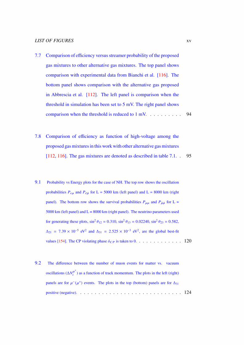
7.7 Comparison of efficiency versus streamer probability of the proposed
gas mixtures to other alternative gas mixtures. The top panel shows
comparison with experimental data from Bianchi et al. [116]. The
bottom panel shows comparison with the alternative gas proposed
in Abbrescia et al. [112]. The left panel is comparison when the
threshold in simulation has been set to 5 mV. The right panel shows
comparison when the threshold is reduced to 1 mV. . . . . . . . . . 94
7.8 Comparison of efficiency as function of high-voltage among the
proposed gasmixtures in thisworkwith other alternative gasmixtures
[112, 116]. The gas mixtures are denoted as described in table 7.1. . 95
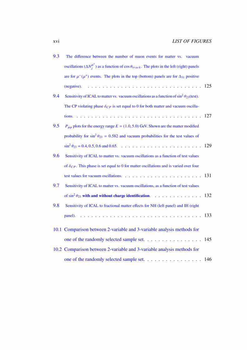
9.1 Probability vs Energy plots for the case of NH. The top row shows the oscillation
probabilities %4` and %4 ¯ for L = 5000 km (left panel) and L = 8000 km (right
panel). The bottom row shows the survival probabilities %`` and % ¯ ¯ for L =
5000 km (left panel) and L = 8000 km (right panel). The neutrino parameters used
for generating these plots, sin2 \12 = 0.310, sin2 \13 = 0.02240, sin2 \23 = 0.582,
Δ21 = 7.39 × 10⁻⁵ eV2 and Δ31 = 2.525 × 10⁻³ eV2, are the global best-fit
values [154]. The CP violating phase X�% is taken to 0. . . . . . . . . . . . . 120
9.2 The difference between the number of muon events for matter vs. vacuum
oscillations (Δ#`∓
8) as a function of track momentum. The plots in the left (right)
panels are for `− (`+) events. The plots in the top (bottom) panels are for Δ31
positive (negative). . . . . . . . . . . . . . . . . . . . . . . . . . . . . 124
xvi LIST OF FIGURES
9.3 The difference between the number of muon events for matter vs. vacuum
oscillations (Δ#`∓
9) as a function of cos \CA02: . The plots in the left (right) panels
are for `− (`+) events. The plots in the top (bottom) panels are for Δ31 positive
(negative). . . . . . . . . . . . . . . . . . . . . . . . . . . . . . . . 125
9.4 Sensitivity of ICAL tomatter vs. vacuumoscillations as a function of sin2 \23(test).
The CP violating phase X�% is set equal to 0 for both matter and vacuum oscilla-
tions. . . . . . . . . . . . . . . . . . . . . . . . . . . . . . . . . . . 127
9.5 %`` plots for the energy range � = (1.0, 5.0) GeV. Shown are the matter modified
probability for sin2 \23 = 0.582 and vacuum probabilities for the test values of
sin2 \23 = 0.4, 0.5, 0.6 and 0.65. . . . . . . . . . . . . . . . . . . . . . . 129
9.6 Sensitivity of ICAL to matter vs. vacuum oscillations as a function of test values
of X�% . This phase is set equal to 0 for matter oscillations and is varied over four
test values for vacuum oscillations. . . . . . . . . . . . . . . . . . . . . . 131
9.7 Sensitivity of ICAL to matter vs. vacuum oscillations, as a function of test values
of sin2 \23 with and without charge identification. . . . . . . . . . . . . . 132
9.8 Sensitivity of ICAL to fractional matter effects for NH (left panel) and IH (right
panel). . . . . . . . . . . . . . . . . . . . . . . . . . . . . . . . . . 133
10.1 Comparison between 2-variable and 3-variable analysis methods for
one of the randomly selected sample set. . . . . . . . . . . . . . . . 145
10.2 Comparison between 2-variable and 3-variable analysis methods for
one of the randomly selected sample set. . . . . . . . . . . . . . . . 146
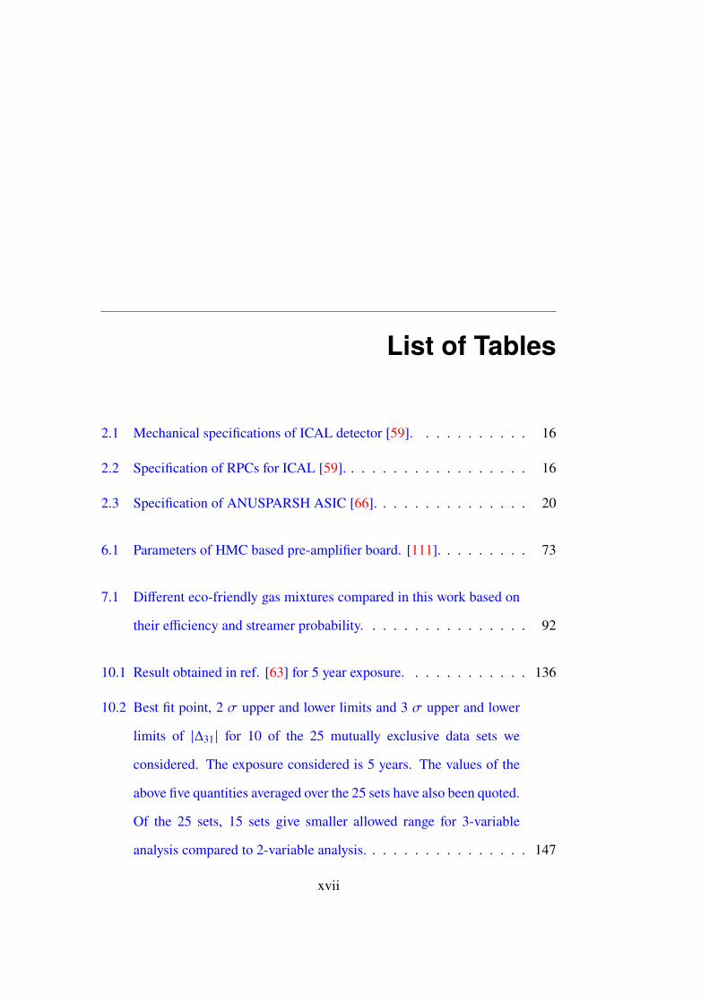
List of Tables
2.1 Mechanical specifications of ICAL detector [59]. . . . . . . . . . . 16
2.2 Specification of RPCs for ICAL [59]. . . . . . . . . . . . . . . . . . 16
2.3 Specification of ANUSPARSH ASIC [66]. . . . . . . . . . . . . . . 20
6.1 Parameters of HMC based pre-amplifier board. [111]. . . . . . . . . 73
7.1 Different eco-friendly gas mixtures compared in this work based on
their efficiency and streamer probability. . . . . . . . . . . . . . . . 92
10.1 Result obtained in ref. [63] for 5 year exposure. . . . . . . . . . . . 136
10.2 Best fit point, 2 f upper and lower limits and 3 f upper and lower
limits of |Δ31 | for 10 of the 25 mutually exclusive data sets we
considered. The exposure considered is 5 years. The values of the
above five quantities averaged over the 25 sets have also been quoted.
Of the 25 sets, 15 sets give smaller allowed range for 3-variable
analysis compared to 2-variable analysis. . . . . . . . . . . . . . . . 147
xvii
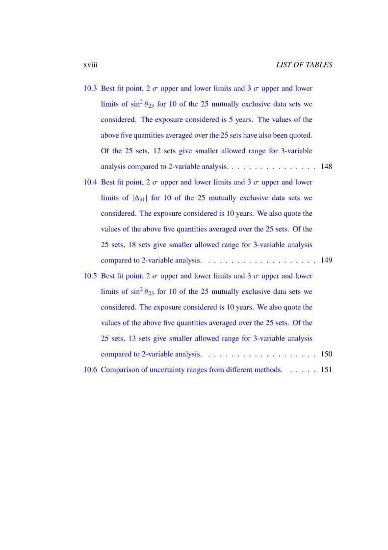
xviii LIST OF TABLES
10.3 Best fit point, 2 f upper and lower limits and 3 f upper and lower
limits of sin2 \23 for 10 of the 25 mutually exclusive data sets we
considered. The exposure considered is 5 years. The values of the
above five quantities averaged over the 25 sets have also been quoted.
Of the 25 sets, 12 sets give smaller allowed range for 3-variable
analysis compared to 2-variable analysis. . . . . . . . . . . . . . . . 148
10.4 Best fit point, 2 f upper and lower limits and 3 f upper and lower
limits of |Δ31 | for 10 of the 25 mutually exclusive data sets we
considered. The exposure considered is 10 years. We also quote the
values of the above five quantities averaged over the 25 sets. Of the
25 sets, 18 sets give smaller allowed range for 3-variable analysis
compared to 2-variable analysis. . . . . . . . . . . . . . . . . . . . 149
10.5 Best fit point, 2 f upper and lower limits and 3 f upper and lower
limits of sin2 \23 for 10 of the 25 mutually exclusive data sets we
considered. The exposure considered is 10 years. We also quote the
values of the above five quantities averaged over the 25 sets. Of the
25 sets, 13 sets give smaller allowed range for 3-variable analysis
compared to 2-variable analysis. . . . . . . . . . . . . . . . . . . . 150
10.6 Comparison of uncertainty ranges from different methods. . . . . . 151

List of Abbreviations
ASCII American Standard Code for Information Interchange
ASIC Application-Specific Integrated Circuit
CC Charged Current
CLS Closed Loop System
FPGA Field Programmable Gate Array
GTLB Global Trigger Logic Board
GWP Global Warming Potential
HMC Hybrid Micro Circuit
ICAL Iron Calorimeter
IH Inverted Hierarchy
IMB Irvine-Michigan-Brookhaven
xix

xx List of Abbreviations
INO India-based Neutrino Observatory
KAMLand Kamioka Liquid Scintillator Anti-neutrino Detector
LVDS Low Voltage Differential Signal
MFC Mass Flow Controller
MINOS Main Injector Neutrino Oscillation Search
MSW Mikheyev-Smirnov-Wolfenstein
NC Neutral Current
NH Normal Hierarchy
NOaA NuMI Off-Axis a4 Appearance
PMNS Pontecorvo-Maki-Nakagawa-Sakata
PMT Photo Multiplier Tube
PREM Preliminary Reference Earth Model
RPC Resistive Plate Chamber
SK Super-Kamiokande
SM Standard Model
SNO Sudbary Neutrino Observatory
SRB Signal Router Board
T2K Tokai to Kamioka

List of Abbreviations xxi
TDC Time-to-Digital Converter
TLB Trigger Logic Board

xxii List of Abbreviations
Chapter 1Introduction
Human civilization has come a long way since the discovery of fire. Our in-
domitable curiosity has driven us from the depth of the sea to the core of the star
in search for answers to the unknowns. It has given birth to different disciplines
for exploring our mother nature, of which physics is one. Knowing the past,
understanding the present and predicting the future of our universe is the soul
of physics. After centuries of hard work, now we are at a stage where we can
dare to claim that we understand a little of our universe. We have come a long
way to perceive the fundamental forces and developed a framework to describe
most of the universe. This well accepted framework, namely the Standard Model
(SM) [1, 2], says that our universe, no matter how diverse it seems, is built of
a few elementary particles as shown in figure 1.1. Depending on their intrinsic
property, called spin, these elementary particles can be divided into two classes:
fermions and bosons. QuantumField theory proposes that every particle, whether
boson or fermion, should have an anti-particle. According to the SM, the vector
bosons mediate the fundamental interactions. For example, the electromagnetic
1

2 CHAPTER 1. INTRODUCTION
Figure 1.1: A schematic representation of Standard Model [1].
interaction is mediated by photon, the weak interactions by Z◦, W+ and W− and
the strong interactions by gluons [2]. The SM also contains a spin zero boson
called the Higgs boson, which is responsible for the mass of all the particles [3].
There are twelve elementary fermions in the Standard model, along with their
anti-particles. They can be further divided into two sectors, known as quarks
and leptons. It has been experimentally established that each of these sectors
consists of three families [4, 5, 6, 7, 8]. For example, the electron, muon and tau
families belong to the leptonic sector. Moreover, each of these families consists
3
of an electrically charged and a neutral member, and the family name is derived
following the charged member. The electrically neutral leptons are known as
neutrinos, who naturally don’t take part in electromagnetic interactions. How-
ever, it has been also established that neutrinos take part in weak interactions but
remain unresponsive to strong interactions [9]. They are mass-less particles as
described by the SM. Following their family name, commonly known as flavor,
the neutrinos are labeled as electron neutrino (a4), muon neutrino (a`) and tau
neutrino (ag).
In the year 1930, Wolfgang Pauli proposed the existence of neutrino, an
electrically neutral, mass-less particle to explain the beta-decay spectrum. Ini-
tially named as "neutron", it was later called "neutrino" following Enrico Fermi’s
proposal to distinguish it from the heavier electrically neutral nucleon, known
as neutron, discovered by James Chadwick in the year 1932. In the year 1956,
Clyde Cowan, Frederick Reines, F. B. Harrison, H.W. Kruse, and A. D.McGuire
announced the detection of neutrino [10]. In 1962, discovery of a` proved the
existence of more than one species of neutrinos [11]. Later, the Large Electron
Positron (LEP) collider measured the invisible decay width of Z◦ boson and
established that there are three light neutrino species [4, 5, 6, 7, 8]. The third
species, ag was later discovered in the year 2000 by the DONUT collaboration
[12] at Fermilab. Since then, neutrinos have always remained at the forefront
of physics and played the role of a probe to the yet undiscovered side of our
Universe.
Since neutrinos react only weakly, they form the best probe available to
understand stars and other stellar objects. A model was built which predicted
that a huge number of neutrinos should be generated as a consequence of the
4 CHAPTER 1. INTRODUCTION
nuclear reactions going on inside the Sun [13, 14]. To establish the solar model,
experiments were designed to measure the neutrino flux emanating from the
Sun. The famous Homestake experiment measured the solar neutrino flux and
observed only a third of the predicted flux [15]. To explain this discrepancy,
different solutions were put forward. Some of these solutions doubted the solar
model, some suspected the nuclear reactionmodels, and others raised the question
of non-standard neutrino properties. The latter included propositions of vacuum
oscillation of neutrinos [16], precision of neutrino spin in the magnetic field of
the Sun [17, 18], neutrino decay [19, 20] and even neutrino oscillation assuming
the oscillation length comparable to the Sun to Earth distance [21]. But all these
solutions have one important requirement, that the neutrinos must have mass.
Later, different experiments, such as Kamiokande II, SAGE, Gallex, SNO, Super-
Kamiokande (SK) ruled out most of the solutions [22]. With the production of
the first SK data, the Mikheyev-Smirnov-Wolfenstein (MSW) solution [23, 24,
25, 26] of the solar neutrino problem received a wide acceptance [27]. Later in
the year 2001, the Sudbury Neutrino Observatory (SNO) established the neutrino
oscillation phenomena as well as the MSW solution, which proved the massive
nature of neutrinos implicitly [28, 29].
Experimentally, it has been established that only left-handed neutrinos and
right-handed anti-neutrinos exist [30]. To explain neutrino mass, two theories
were put forward. One of them proposes that neutrinos are Dirac particle,
which means that the neutrinos and anti-neutrinos are separate particles and
the right-handed neutrinos and left-handed anti-neutrinos don’t interact through
SM gauge bosons. The other proposition says that they are Majorana particles,
implying neutrinos and anti-neutrinos are the same particles. In case of massive
5
neutrinos, it was proposed that the flavor eigenstates of neutrinos need not be
mass eigenstates, but instead are a superposition of the mass eigenstates [16, 31,
32]. Maki, Nakagawa and Sakata formulated themixing between flavor states and
proposed a unitary matrix known as PMNS matrix. Like every unitary matrix,
PMNS matrix can be parameterized using nine parameters: three mixing angles
and six phases. Out of the six phases, three can be absorbed in the neutrino
flavor eigenstates irrespective of the Dirac and Majorana nature of neutrinos.
If neutrinos are Dirac particles, two more phases can be absorbed in neutrino
mass eigenstates and the sixth one is responsible for CP violation, which is
denoted as X�%. The three mixing angles are denoted as \12, \23 and \13. In the
course of propagation of a flavor eigenstate, different mass eigenstates pick up
different phases due to time evolution. This time evolution phase is dependent
on the mass square difference of the mass eigenstates, which can be expressed as
Δ8 9 = <28− <2
9, where 8, 9 = 1, 2, 3, and 8 > 9 . This phase is responsible for
the neutrino oscillation.
Following the PMNS paradigm, the oscillation probabilities depend on three
mixing angles, two mass square differences and one CP violating phase. The
mixing angle \12 and the mass square difference Δ21 were determined from
solar neutrino [33, 34, 35, 36, 37, 38] and KamLAND reactor neutrino data
[39, 40, 41]. The CHOOZ reactor neutrino experiment pinned down the value
of \13 [42, 43]. The values of Δ31 and \23 were measured by long-baseline
experiments, like T2K [44], MINOS [45] and atmospheric neutrino experiments,
SK [46], IceCube-DeepCore [47]. The CP violating phase was obtained from
two separate long-baseline experiments, T2K and NOaA though they disagree
about its value. Currently, the value of Δ31 is known, but its sign is yet to
6 CHAPTER 1. INTRODUCTION
be determined. Therefore, it is not yet established whether the mass <3 is the
largest or the smallest. The present time will continue to see many experimental
endeavors to explore the unknown sign of, Δ31 which is commonly known as the
mass hierarchy problem. The case of positive Δ31 is labelled normal hierarchy
(NH) and that of negative Δ31 inverted hierarchy (IH).
Atmospheric neutrinos are the most abundant natural source of neutrinos,
with energy varying from hundreds of MeV to a few Tev. They are generated
in decay of the short-lived particles, like c±, 0 and ±, 0, created in interactions
between cosmic particles and gas molecules present in Earth’s atmosphere. Due
to their short life span, the pions and kaons decay intomuons andmuon neutrinos,
conserving the electrical and leptonic charge of the reaction. The muons created
in these processes can also decay and produce electrons along with electron
neutrinos. All these processes can be expressed as follows
? + 08A → c±, c◦, ±
c+, + → `+ + a`, c−, − → `− + a`
`+ → 4+ + a4 + a`, `− → 4− + a4 + a`
Neutrino flux up to energy of few GeV has negligible contribution of ag flux due
to lack of energy to produce heavy particles such as g. Following the neutrino
generation processes, it is evident that the total a` and a` flux is nearly double
of the total a4 and a4 flux [48]. But this ratio is not constant and heavily depends
upon the neutrino energy Ea as shown in figure 1.2 [48]. The robust calculations
of neutrino flux by different groups predicted up-down symmetry in the flux at
high energy in absence of neutrino oscillation. But initial data from IMB [53,

7
Bartol
Fluka
HKKMS06
HKKM11
Figure 1.2: Neutrino flux ratio as function of Ea calculated by Bartol group [49],Fluka Group [50], HKKMS06 [51] and HKKM11 [52] for the Kamioka site,Japan [48].
54] and Kamiokande [55, 56] did not observe such symmetry in atmospheric
muon neutrino fluxes. Later, SK [57] measured the zenith angle dependence of
atmospheric muon and electron neutrinos and established atmospheric neutrino
oscillations. These detectors are placed underground and observe neutrinos
coming from all the sides. The neutrinos which are coming from top and going
downwards reaches to the detector after traversing the atmospheric height which
maximally 20 km. But the neutrinos which are coming from bottom and going
upward with respect to the detector traverse the whole Earth and a path of about
12756 km. So, these detectors observed neutrinos which traverse path lengths (L)
of few km to thousands of km. This huge L/Ea spectrum available for atmospheric
neutrinos makes them an excellent probe to explore neutrino oscillation. The
result from SK [57] established that the atmospheric muon neutrino oscillation is
8 CHAPTER 1. INTRODUCTION
governed by the parameters Δ31 and \23. The Earth-matter potential modifies the
oscillation probabilities of the neutrino and its anti-particle in completely opposite
way, depending on the sign of the parameter Δ31. Therefore, the measurement
of neutrino and anti-neutrino fluxes traversing through the Earth can give an
important lead towards the determination of the sign of Δ31. Moreover, this
huge L/Ea spectrum available for atmospheric neutrinos makes the observed
data insensitive to the yet to be measured CP violating phase, which can mimic
the Earth matter effect in neutrino oscillation [58]. So, exploring the Earth
matter effect on atmospheric neutrino flux can solve the neutrino mass hierarchy
problem, which motivated the idea of ICAL at INO.
India-based Neutrino Observatory (INO) [59] is an underground facility pro-
posed to be constructed for augmenting the research on neutrino physics in India.
The facility will be built under the West Bodi Hills, situated at Theni district
in the state of Tamilnadu. Iron Calorimeter (ICAL) is one of the experiments
that will be housed in this upcoming facility with an objective of studying the
atmospheric neutrinos, which are the decay product of the particles created in
reactions between cosmic particles and atmospheric gas molecules. The atmo-
spheric neutrino energy spectrum spans from hundreds of MeV to a few TeVwith
the flux peaking at around an order of 1 GeV. After the peak, the neutrino flux
falls down following E−2.7a , where Ea is the neutrino energy. ICAL is a calorime-
ter with tracking capabilities that has been designed to explore the Earth-matter
effect on neutrino oscillation by studying the energy and zenith angle dependent
flux of the atmospheric muon neutrinos (a`) and muon anti-neutrinos (a`). This
study will help in the determination of the sign of the mass squared difference,
Δ31 (= <23 − <
21) which is an important observable among several others of this
9
experiment. The Earth-matter affects the oscillation probabilities of a`/a` in
opposite way depending upon the sign of the parameter Δ31. Thus, the measure-
ment of their fluxes has been considered as an important key requirement in the
design and operation of ICAL. Eventually, the ICAL has been conceived as a
tracking calorimeter with layers of iron slabs as the target material and Resistive
Plate Chamber (RPC), interleaved with the iron slabs as the active component
for tracking the charged leptons created in the charged current (CC) interactions
between the neutrinos and iron nuclei. The charged leptons of opposite electri-
cal charges produced by the CC interaction of a` and a` will be distinguished
by application of a magnetic field across the ICAL. It will not only facilitate
observing the Earth-matter effect on neutrino and anti-neutrino separately, but
also determination of their energy from the curvature of the track of the charged
leptons. The details of the ICAL detector will be discussed in chapter 2 and
the simulation methods used to carry out its performance will be described in
chapter 3.
The present doctoral work focuses on improvement of several aspects related
to the future operation and performance of the ICAL experiment. The topics can
be briefly mentioned as follows.
• Exploration for alternative gas mixtures of the RPCs:- The RPCs of
the ICAL foresee a long-term operation in order to accumulate substantial
statistics to achieve the experimental objectives. Alongside, the detectors
should perform with spatial resolution of about 1 cm for reliable track
reconstruction and time resolution of 1 ns to precisely determine the direc-
tion of the neutrinos (upward or downward). The RPC when operated in
10 CHAPTER 1. INTRODUCTION
avalanche mode with a gas mixture composed of 1,1,1,2-Tetrafluoroethane
(R134a) (95.2%), isobutane (i-C4H10) (4.5%) and sulfur hexafluoride (SF6)
(0.3%) has been found to fulfill the experimental performance requirement.
However, the high Global Warming Potential (GWP) of the R134a and the
SF6, which are 1300 and 23900, respectively, along with that of i-C4H10
being 3 makes the effective GWP of the said gas mixture little more than
1300. It is well beyond the permissible limit of 150, set by the Kyoto proto-
col [60], adopted in 1997 by the United Nations Framework Convention on
Climate Change (UNFCCC) in order to limit and reduce greenhouse gas
emissions. It certainly calls for an exploration of alternative gas mixtures
with sufficiently low GWP for operating the RPCs without compromising
the objectives of the ICAL experiment. The first part of the doctoral thesis
will discuss how the issue of identifying an alternative eco-friendly gas
mixture has been addressed with a numerical model developed for emulat-
ing the device dynamics of RPC configured for the ICAL. In this context,
the details of the design and working of RPC will be introduced in chapter
4. In chapter 5 the numerical model framed on the basis of hydrodynamic
approach to reproduce the RPC performance will be described. Its compar-
ison with available experimental data will also be reported to demonstrate
its efficacy. The performance of the model has been verified in case of the
RPCs of ICAL by comparing its results to the experimental measurements
done with an RPC prototype. The procedure of the prototype fabrication
and its test will be furnished in chapter 6. Finally, in chapter 7, an eco-
friendly gas mixture proposed in this doctoral work for the avalanche mode
operation of the RPC in the ICAL will be evaluated for its credibility using
11
the validated numerical model.
• Discrimination of matter effect from vacuum oscillation in atmo-
spheric neutrino oscillation:- Neutrino oscillations governed by Δ31 and
sin2 \23 are well established by several long baseline and atmospheric neu-
trino experiments which look at a`/a` disappearance data. In all these
experiments, the neutrinos traverse through the Earth-matter. Though the
presence of matter in the path of the neutrino modifies the oscillation
probability, the data of these experiments, when fitted with the vacuum os-
cillation hypothesis, returned a good fit. Till now, only the analysis of the
SK experimental data was able to discriminate the matter oscillation hy-
pothesis from vacuum oscillation, with only 1.6 f significance. The a4/a4
appearance data obtained from long baseline experiments can discriminate
the vacuum and matter oscillation hypotheses, but that signal can be mim-
icked by CP violation. This made the effect of CP violation and matter
oscillation hypothesis entangled. To disentangle this degeneracy, different
experiments should establish the matter oscillation hypothesis first. The
next part of the doctoral thesis has studied the reach of the ICAL in this
direction. Chapter 8 will describe the matter and vacuum oscillation hy-
potheses, followed by the discussion on the work and the results presented
in chapter 9.
• Determination of neutrino oscillation parameters using track and hit
information from GEANT4:- In the analysis methods developed earlier
[61, 62] to determine |Δ31 | and sin2 \23 considered detector response with
smearing instead of using full-fledged GEANT4 reconstruction. A re-

12 CHAPTER 1. INTRODUCTION
cent work by Rebin et al. [63] used muon information reconstructed by
GEANT4 to determine these parameters and also the effect of fluctuation
in the data, which have made the analysis method more realistic. In this
work, hadron information has been incorporated in addition, which has
been found to improve the precision. Chapter 10 will present the details of
this work and the relevant results.
The doctoral thesis will end with Chapter 11 which will contain the final remarks
about these studies carried out for the ICAL experiment and discuss the future
scopes arising out of these endeavors.

Chapter 2Iron Calorimeter Detector
INO is an underground facility that would be built to house different experiments,
which will require substantial background suppression. Some notable as exper-
iments would be to study neutrino-less double beta decay, dark matter etc. The
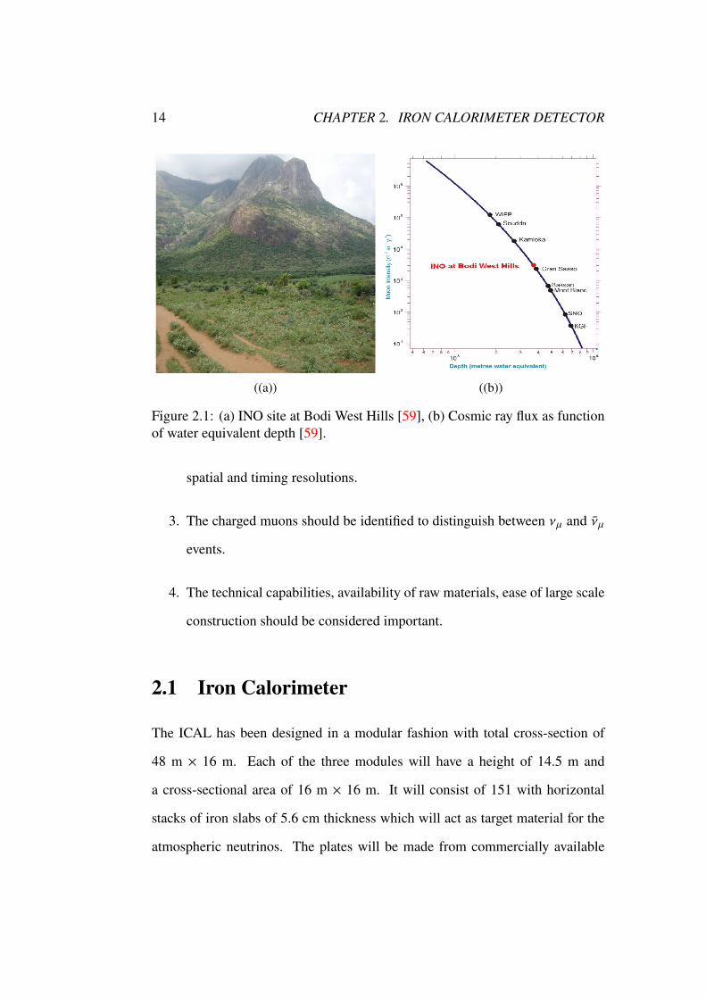
natural stone coverage of Bodi West Hills depicted in figure 2.1(a) from all sides
would reduce the cosmic ray flux below 103 m−2sr−1yr−1, shown in figure 2.1(b)
and thus improve the sensitivity of the measurements [59].
ICAL would be a major experimental setup at INO which will primarily be
dedicated for determination of neutrino mass hierarchy along with investigations
related to other important aspects of neutrino oscillation phenomenon. The key
factors that have governed the concept of the ICAL detector are the following.
1. A large target mass is required to achieve significant statistics of neutrino
events within a reasonable time period for observation of neutrino oscilla-
tion.
2. The energy Ea and the path-length L need to be accurately measured to
detect the oscillation pattern in L/Ea spectrum, which necessitates good
13
14 CHAPTER 2. IRON CALORIMETER DETECTOR
((a)) ((b))
Figure 2.1: (a) INO site at Bodi West Hills [59], (b) Cosmic ray flux as functionof water equivalent depth [59].
spatial and timing resolutions.
3. The charged muons should be identified to distinguish between a` and a`
events.
4. The technical capabilities, availability of raw materials, ease of large scale
construction should be considered important.
2.1 Iron Calorimeter
The ICAL has been designed in a modular fashion with total cross-section of
48 m × 16 m. Each of the three modules will have a height of 14.5 m and
a cross-sectional area of 16 m × 16 m. It will consist of 151 with horizontal
stacks of iron slabs of 5.6 cm thickness which will act as target material for the
atmospheric neutrinos. The plates will be made from commercially available
2.1. IRON CALORIMETER 15
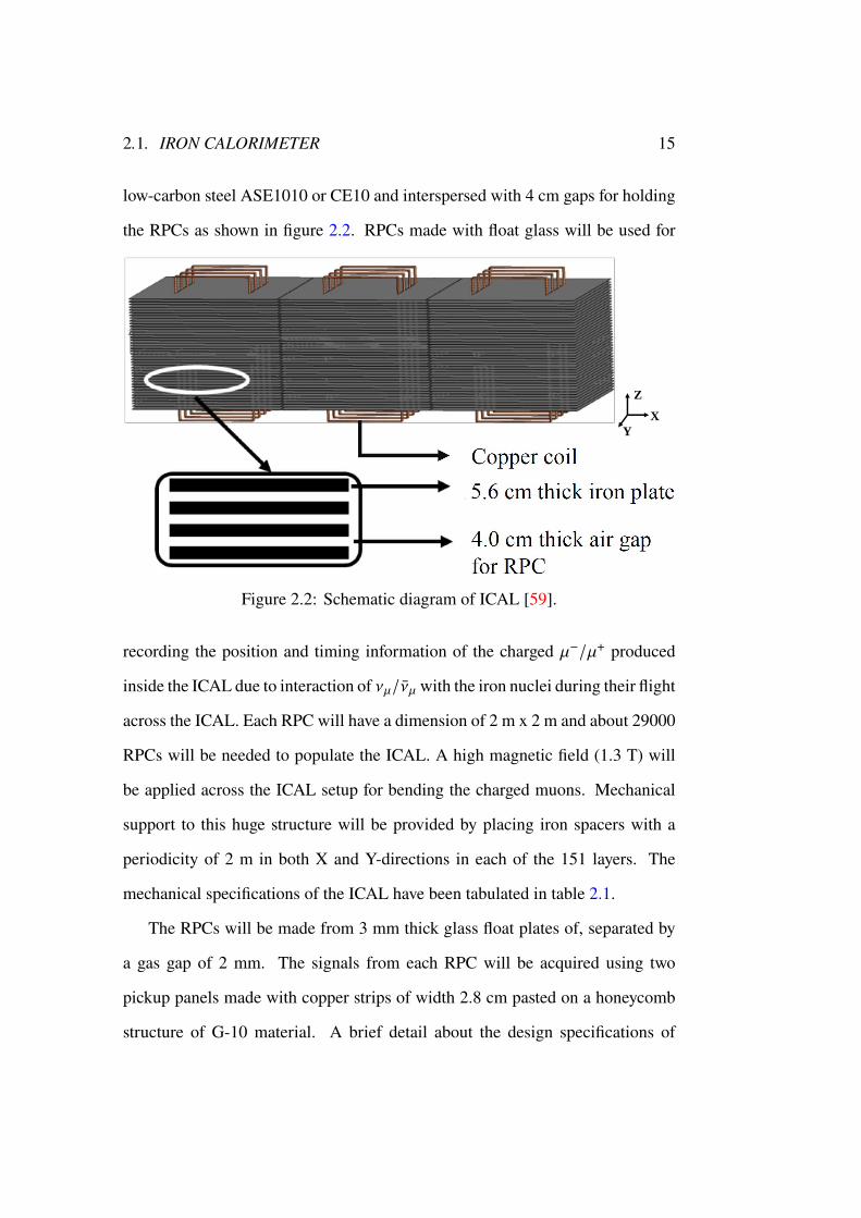
low-carbon steel ASE1010 or CE10 and interspersed with 4 cm gaps for holding
the RPCs as shown in figure 2.2. RPCs made with float glass will be used for
Z
X
Y
Figure 2.2: Schematic diagram of ICAL [59].
recording the position and timing information of the charged `−/`+ produced
inside the ICAL due to interaction of a`/a` with the iron nuclei during their flight
across the ICAL. Each RPC will have a dimension of 2 m x 2 m and about 29000
RPCs will be needed to populate the ICAL. A high magnetic field (1.3 T) will
be applied across the ICAL setup for bending the charged muons. Mechanical
support to this huge structure will be provided by placing iron spacers with a
periodicity of 2 m in both X and Y-directions in each of the 151 layers. The
mechanical specifications of the ICAL have been tabulated in table 2.1.
The RPCs will be made from 3 mm thick glass float plates of, separated by
a gas gap of 2 mm. The signals from each RPC will be acquired using two
pickup panels made with copper strips of width 2.8 cm pasted on a honeycomb
structure of G-10 material. A brief detail about the design specifications of
16 CHAPTER 2. IRON CALORIMETER DETECTOR
Number of Modules 3Dimension of each Module 16 m × 16 m × 14.5 m
Dimension of total ICAL detector 48 m × 16 m × 14.5 mNumber of layers per Module 151Thickness of each Iron plate 5.6 cmSpace between two Iron plates 4.0 cm
Magnetic Field ∼1.3 T
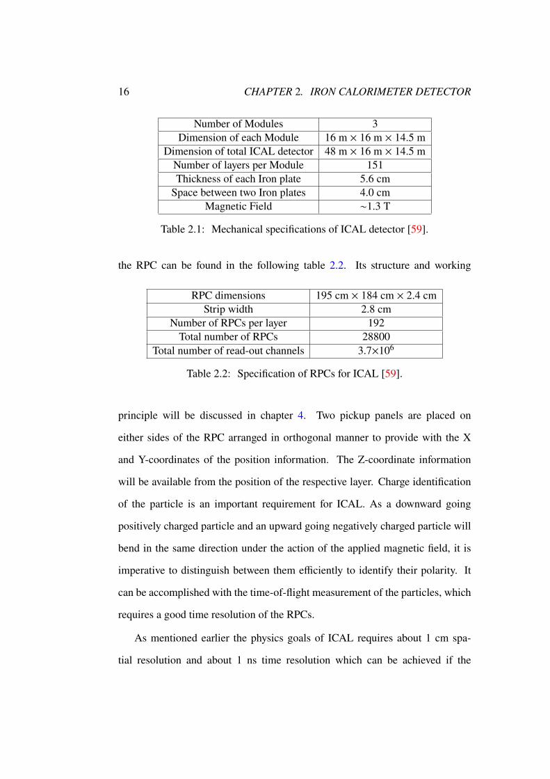
Table 2.1: Mechanical specifications of ICAL detector [59].
the RPC can be found in the following table 2.2. Its structure and working
RPC dimensions 195 cm × 184 cm × 2.4 cmStrip width 2.8 cm
Number of RPCs per layer 192Total number of RPCs 28800
Total number of read-out channels 3.7×10⁶
Table 2.2: Specification of RPCs for ICAL [59].
principle will be discussed in chapter 4. Two pickup panels are placed on
either sides of the RPC arranged in orthogonal manner to provide with the X
and Y-coordinates of the position information. The Z-coordinate information
will be available from the position of the respective layer. Charge identification
of the particle is an important requirement for ICAL. As a downward going
positively charged particle and an upward going negatively charged particle will
bend in the same direction under the action of the applied magnetic field, it is
imperative to distinguish between them efficiently to identify their polarity. It
can be accomplished with the time-of-flight measurement of the particles, which
requires a good time resolution of the RPCs.
As mentioned earlier the physics goals of ICAL requires about 1 cm spa-
tial resolution and about 1 ns time resolution which can be achieved if the
2.1. IRON CALORIMETER 17
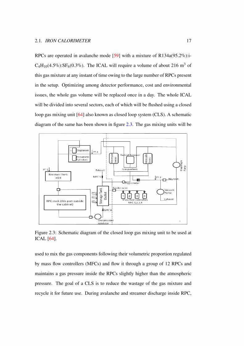
RPCs are operated in avalanche mode [59] with a mixture of R134a(95.2%):i-
C4H10(4.5%):SF6(0.3%). The ICAL will require a volume of about 216 m3 of
this gas mixture at any instant of time owing to the large number of RPCs present
in the setup. Optimizing among detector performance, cost and environmental
issues, the whole gas volume will be replaced once in a day. The whole ICAL
will be divided into several sectors, each of which will be flushed using a closed
loop gas mixing unit [64] also known as closed loop system (CLS). A schematic
diagram of the same has been shown in figure 2.3. The gas mixing units will be
Figure 2.3: Schematic diagram of the closed loop gas mixing unit to be used atICAL [64].
used to mix the gas components following their volumetric proportion regulated
by mass flow controllers (MFCs) and flow it through a group of 12 RPCs and
maintains a gas pressure inside the RPCs slightly higher than the atmospheric
pressure. The goal of a CLS is to reduce the wastage of the gas mixture and
recycle it for future use. During avalanche and streamer discharge inside RPC,

18 CHAPTER 2. IRON CALORIMETER DETECTOR
many radicals are created, which can deteriorate the detector health if they are
not removed from the system. So, using a pneumatically controlled positive dis-
placement pump, the used gas mixture stored in the receiver tank at RPC outlet,
is sucked and sent to the radical removers. There, other than the radicals, excess
water vapor is also removed. This process is donemaintaining a pressure between
1015mbar and 1018mbar in the receiver tank. Less pressure than 1015mbar will
allow to drop the pressure inside the RPC also, which will let atmospheric gas
to enter the detector and contaminate it. More than 1018 mbar may damage the
detector health due to high pressure. Once the radicals are removed, the purified
gas mixture is sent to the storage tank, from which the gas is resupplied to the
RPCs. The pressure in the storage tank is maintained at 1650 mbar, and it is kept
isolated from the RPCs by an MFC so that the high pressure is not realized by the
RPCs. The drop in RPC pressure will open the low-pressure regulator and the
gas mixture will be delivered to the RPC stack. Once the pressure in the storage
tank falls below 1350 mbar, the MFCs connected to different gas cylinders starts
working and let pure gases to enter the storage tank, maintaining the desired
volumetric proportion of the component gases. The filling up continues till the
pressure reaches 1650 mbar, more than that opens the exhaust and excess gas is
released.
2.2 Magnet of ICAL
Depending on the mass hierarchy of the neutrinos, the resonance effect due to
Earth-matter occurs either in neutrinos or in anti-neutrinos. In case of Normal
Hierarchy (NH), the resonance is present in neutrinos and for Inverted Hierarchy
2.2. MAGNET OF ICAL 19
(IH), it is observed in case of anti-neutrinos. So, measuring the neutrino and
anti-neutrino interaction rates individually is themost important goal of the ICAL
detector. Here the magnetic field plays a crucial role as it makes the track of the
charged muons to bend differently depending on their polarity. Also, the radius
of curvature of the track depends on the momentum of the charged muon. As the
momentum information of the charged muons is important for the determination
of the mass hierarchy, uniformity of the magnetic field is essential to ensure
precision in the measurement. Apart from this, several technical issues, like ease
of handling and optimization between themagnetic field and power consumption,
have governed the design criteria of the electromagnets used in ICAL.
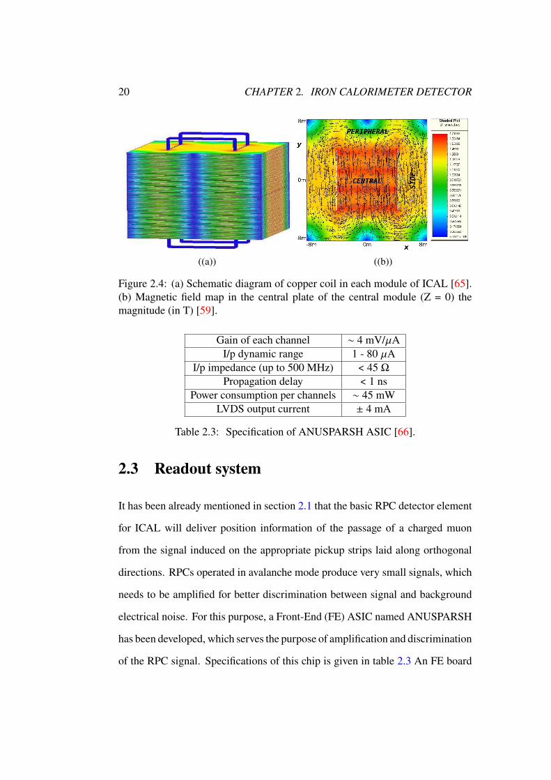
A toroidal design of the electromagnet made of copper coils has been opted
for the ICAL. A small cross-section of 1 cm × 1 cm with small width of 20 cm
of the coils has ensured the required magnetic field with minimum loss of active
volume of the detector. The coils will pass through two rectangular slots in the
stack of the iron plates. To produce a magnetic field of 1.3 T, a copper coil of
40000 amp-turns is deployed in each module of the detector. Figure 2.4(a) shows
the schematic diagram of the electromagnet of a single module of the ICAL
detector. The magnetic field distribution in each layer of the module has been
depicted in figure 2.4(b). It has been found that. The magnetic field varies by less
than 0.15% over a depth of ± 5 m in Z-direction from the center of the module.
Though the variation of magnetic field in X-direction is less than 0.25%, but they
fall rapidly outside the coil set (± 4 m) in Y-direction.
20 CHAPTER 2. IRON CALORIMETER DETECTOR
((a)) ((b))
Figure 2.4: (a) Schematic diagram of copper coil in each module of ICAL [65].(b) Magnetic field map in the central plate of the central module (Z = 0) themagnitude (in T) [59].
Gain of each channel ∼ 4 mV/`AI/p dynamic range 1 - 80 `A
I/p impedance (up to 500 MHz) < 45 ΩPropagation delay < 1 ns
Power consumption per channels ∼ 45 mWLVDS output current ± 4 mA
Table 2.3: Specification of ANUSPARSH ASIC [66].
2.3 Readout system
It has been already mentioned in section 2.1 that the basic RPC detector element
for ICAL will deliver position information of the passage of a charged muon
from the signal induced on the appropriate pickup strips laid along orthogonal
directions. RPCs operated in avalanche mode produce very small signals, which
needs to be amplified for better discrimination between signal and background
electrical noise. For this purpose, a Front-End (FE) ASIC named ANUSPARSH
has been developed, which serves the purpose of amplification and discrimination
of the RPC signal. Specifications of this chip is given in table 2.3 An FE board
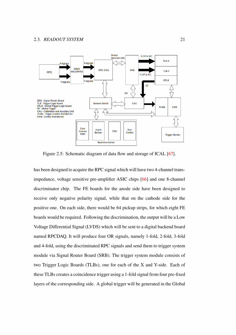
2.3. READOUT SYSTEM 21
Figure 2.5: Schematic diagram of data flow and storage of ICAL [67].
has been designed to acquire the RPC signal which will have two 4-channel trans-
impedance, voltage sensitive pre-amplifier ASIC chips [66] and one 8-channel
discriminator chip. The FE boards for the anode side have been designed to
receive only negative polarity signal, while that on the cathode side for the
positive one. On each side, there would be 64 pickup strips, for which eight FE
boards would be required. Following the discrimination, the output will be a Low
Voltage Differential Signal (LVDS) which will be sent to a digital backend board
named RPCDAQ. It will produce four OR signals, namely 1-fold, 2-fold, 3-fold
and 4-fold, using the discriminated RPC signals and send them to trigger system
module via Signal Router Board (SRB). The trigger system module consists of
two Trigger Logic Boards (TLBs), one for each of the X and Y-side. Each of
these TLBs creates a coincidence trigger using a 1-fold signal from four pre-fixed
layers of the corresponding side. A global trigger will be generated in the Global
22 CHAPTER 2. IRON CALORIMETER DETECTOR
Trigger Logic Board (GTLB) by carrying out OR operation on these two trigger
signals from X and Y-side TLBs. It will initiate recording of the data in the
RPCDAQ board once the trigger is received. Subsequently, it will be passed
on to data concentrator and Event Builder via Network Switch. The output of
this step will be stored in a computer for further analysis. The schematic of the
readout and data collection is shown in the figure 2.5. Details of these processes
can be found in [68, 69, 70].
It can be followed from the discussions made in this chapter that the ICAL
has been designed following the requirement to make it sensitive to the energy,
direction and sign of the electric charge of the muons that are produced in the
CC interaction of the detector material with the atmospheric neutrinos. In the
next chapter, the simulated performance of the ICAL will be discussed, which
is important to judge the scope of the detector system in achieving the desired
objectives of neutrino oscillation experiment.
Chapter 3Simulation Framework of ICAL
The ICAL experiment will explore the Earth matter effect on the neutrino oscilla-
tion by studying the dependence of multi GeV atmospheric a/a fluxes on zenith
angle and energy [59]. The unique capability of the detector to discriminate
neutrinos from anti-neutrinos makes it a contender of solving the long-standing
neutrino mass hierarchy problem. The final state particles created in neutrino-
nuclei interactions in the detector will be studied to extract information about
the parent neutrinos. So, precise measurement of energy and direction of the
final state charged particles will be crucial for the experiment. This demands a
careful and detailed calibration of the detector beforehand, which can be useful in
predicting and interpreting the actual experimental data. In this chapter, a brief
discussion will be made about the ICAL simulation framework which is used
to carry out a realistic numerical experiment incorporating ICAL geometry and
RPC properties to find out the response of ICAL to the atmospheric a/a fluxes.
It provides an assessment of the potential of ICAL to measure the dependence
of these on zenith angle and energy. A schematic flow-chart of the simulation
23
24 CHAPTER 3. SIMULATION FRAMEWORK OF ICAL
framework has been shown in figure 3.1 where all the steps taken to accomplish
the simulation in general have been broadly classified into several blocks. In
the following sections, each of the blocks will be discussed in reference to the
present doctoral work.
3.1 Event Generation
The simulation framework starts with an event generator which creates neutrino
events using atmospheric neutrino flux and propagates the neutrinos to let them
interact with the detector. The neutrino cross-sections are stored as internal
libraries in the generator, and the events are generated for a given number or an
exposure time. There are many neutrino generators available, like ANIS [71],
FLUKA routines [50], GiBBU [72, 73], GENIE [74], NEUT [75], NUANCE
[76], NEGN [77], etc. which are basically Monte-Carlo programs. In this doc-
toral work, NUANCE has been used as the event generator, which is a FORTRAN
based program. It was originally developed by Dave Casper to generate events
for the simulation of SK experiment. A simple model of ICAL geometry and
the neutrino flux observed at Kamioka site have been subjected to simulate the
interaction of the neutrinos with the ICAL. NUANCE has returned information
about the parent neutrinos along with their interaction vertex and the momentum
and identity of the final products in ASCII format. The ASCII file has been
imported to C++ based GEANT4 package [78] for carrying out the next steps
of event simulation, digitization and reconstruction. Several interaction mecha-
nisms, such as Quasi Elastic (QE), Resonance (RES), Deep Inelastic Scattering
(DIS), coherent nuclear processes on nuclei, neutrino-electron elastic scattering
3.1. EVENT GENERATION 25
Event Generation
• Uses detector geometry, atmospheric neutrino flux and neutrino interaction cross-sections to generate events.
• Returns the interaction vertex information, energy, momentum and identity of final state particles.
Event Simulation
• Uses the output information of event generator.
• Propagates the final state particles through the detector geometry and produces the X, Y, Z-coordinates and time stamp of the particle-hits.
Event Digitization
• Uses hit pattern of each particle and incorporates detector properties.
• Returns strip positions corresponding to the particle-hits
Event Reconstruction
• Sifts through the digitized hits and reconstructs the track of each particle.
• Reconstructs energy, electrical charge and direction of the particles and stores with time and event stamps.
Analysis
• Uses the stored output of reconstructed events.
• Analyses stored data using different user-specific methods to estimate ICAL’s reach for different phenomena.
Figure 3.1: Schematic of the ICAL simulation framework.
26 CHAPTER 3. SIMULATION FRAMEWORK OF ICAL
and inverse muon decay [76] are considered. The event generator can also gen-
erate an oscillated event spectrum, for which it assumes Earth as a system of
25 concentric shells of constant density. To reduce the computational expense
and complexity in calculation, this option has not been exercised in the present
simulation. In the following sections, the subsequent steps of the simulation
work carried out using the GEANT4 package will be discussed.
3.2 Event Simulation and Digitization
At this stage, the event simulation starts with shooting the final state particles
of neutrino interaction with their momentum and energy as provided by the
event generator. In this work, the particles produced at different interaction
vertices with given momentum and energy as provided by NUANCE have been
propagated and the GEANT4 has calculated energy deposition by them in the
ICAL setup. To accomplish this, a machine-readable file containing the ICAL
detector geometry, interaction cross-sections of different particles and various
physics models have been considered. The geometry file of the ICAL contains
the relevant details, such as thickness and position of iron slabs, position of copper
coils for themagnet, design parameters of the RPCs including their copper pickup
strips and gas mixture, and the support structure of each module of the ICAL.
The magnetic field distribution in each module has been also incorporated in the
detailed information of the ICAL. All the particles have been tracked till they have
stopped in the ICAL or left the detector. A minimum cutoff energy has been set
to determine the location of their stopping, while the particles that have escaped
the detector have been tracked till the boundary. The RPC has been considered
3.3. EVENT RECONSTRUCTION 27
to register a hit if any charged particle deposits more than 30 eV in the detector
gas gap. A detector efficiency of 95% also has been incorporated to mimic the
realistic detector performance. The corresponding X, Y and Z-coordinates of
each hit in the RPC with the time and event stamp have been stored and digitized
subsequently.
In the digitization stage, the RPC properties, such as spatial resolution, cross
talk between the pickup strips, multiplicity of the detector and its time resolution
are required to translate the simulated hit to 3D position information as would be
recorded by the detector system. Using these parameters from [79] the precise
hit position has been converted to the position of the X and Y pickup strips which
have registered the hit. For obtaining the Z-position of each hit, the vertical
location of the RPC in the ICAL has been recorded.
3.3 Event Reconstruction
In the next step, the tracks of the particles have been reconstructed using the
digitized hits as obtained from different layers of RPC. The event reconstruction
part has been done in two steps, which are namely track finding and track fitting.
These will be discussed in the following subsections.
3.3.1 Track finding
The hits, generated for all the particles of an event, are stored irrespective of
any specific particle or group of particles. In order to reconstruct the track, it is
necessary to identify the hits which belong to the track. For this purpose, all the
adjacent X and Y hits for an event in a layer are first grouped, and this is done for

28 CHAPTER 3. SIMULATION FRAMEWORK OF ICAL
Figure 3.2: An example of simulated a` CC interaction in the detector [81].
all the layers. In the next, the groups of the adjacent layers are then fitted using a
curve fitting program to form tracklets which are subsequently joined to form a
track. These processes are carried out in an iterative manner to form tracks [80].
To identify the direction of the movement of the particle (upward / downward),
time information from each group of different layers are considered. The average
time information of all the X and Y hits of each group has been considered as
the time stamp of the respective group. Usually a muon track is found clean
having one or two hits per layer, while a high energy electron or hadron creates a
shower of hits in the detector. Different hadrons create similar kind of showers,
and identifying the hadron from the shower is not possible as a result. Only the
direction and number of hits for them is stored. A typical case of CC interaction
in the detector has been presented in figure 3.2 where the muon track and the
hadron shower produced from the interaction vertex have been marked.

3.3. EVENT RECONSTRUCTION 29
3.3.2 Track fitting
Following the determination of tracklets, a track fitting algorithm based on
Kalman filter is introduced for the purpose of track finding. It includes the
effect of the magnetic field as the tracks of the charged particle bend under its
influence. The process starts with a state vector
-0 =
(-,.,
3-
3/,3.
3/,@
?
)where X, Y and Z are the hits coordinates and @
?is the ratio of charge and
inverse momentum of the particle at a specific layer. At the beginning the track
is linear and hence the track direction can be found from 3-3/
and 3.3/
of the first
two layers. For further propagation, Kalman gain matrix is calculated. The
calculation incorporates the local magnetic field and geometry of the detector
and uses these to extrapolate the predicted position of the tracklet in the next
layer. While predicting the state vector using Kalman algorithm in the next
layer, noise due to multiple scattering [82] and energy loss of the particle as
described by Bethe formula [83] are incorporated. The error propagation is
implemented by calculating the propagator matrix [80]. Improved formulae for
atmospheric neutrinos [84] have been used for propagation of states and errors.
The extrapolated point is then compared with the actual hit point in that layer if
there has been any and the error is estimated. Following its minimization, the
track is extrapolated back to compare with the earlier hits and estimate the errors
there, which are minimized also. Then again the state vector is propagated for
finding the next hit and the same process is repeated. This iteration continues till
the best fitted track is found. The condition to stop the iteration, that the value
of j2
=35will be less than 10. Subsequently, the fitted track is extrapolated back to
30 CHAPTER 3. SIMULATION FRAMEWORK OF ICAL
find the vertex and the momentum at the vertex is considered as the reconstructed
momentum of that particle. The magnitude of the momentum is saved as, @?with
its sign determined by the polarity of the charge of the particle. From the value
of 3-3/
at the vertex, the direction of the event is determined while the value is
saved as zenith angle \, and from the value of 3.3/
the azimuth angle is calculated
and stored as q.
The muons that are produced in the neutrino-nucleus CC interaction in the
ICAL, are minimum ionizing particles, and so deposit less energy leaving a
long track in the detector. To identify a track produced by muon, a threshold
of 5 hits in the track has been implemented. For other particles, if a track is
reconstructed, information related to it has been also stored in an array where
the longest muon like track is kept as the first entry. To find the hits due to
hadron shower, an algorithm named trapezoidal algorithm [85] is used. Events
with hadrons as final particles can be classified in two categories: one with a
reconstructed track and the other one without any reconstructed track. In case
of a reconstructed track, it is extrapolated back up to six layers and absence of
real hit in the vicinity of extrapolated hits in two consecutive layers terminates
the extrapolation. Around the newly found vertex a trapezoid is formed with its
base of 10 cm. All the hits which are not used in track reconstruction and falls in
this trapezoid are taken as hadron hits. In case of no reconstructed track, first all
the RPCs having the large number of hits (> 100 strips fired) are excluded and
then clusters are formed. Details of ICAL muon response can be found in [59]
following which the reconstruction of the energy of the particles, its electrical
charge and direction are done.
3.4. ANALYSIS METHOD 31
3.4 Analysis Method
With the simulated output, different physics analyses are carried out using ROOT
data analysis framework [86]. For brevity the output of the ICAL simulation
code is stored in .ROOT format, formatted for an object-oriented data analysis
framework, namely ROOT to analyze large amount of data efficiently. The
simulated data are stored in .ROOT format consisting a main section and different
subsections under it denoted as tree and branch respectively. Depending on
the physics topic to be studied, an analysis code is developed which uses the
reconstructed information as described above.
While in propagation, the atmospheric neutrinos oscillate, which changes
the flux of different neutrino flavors. The following section will describe the
procedure followed to incorporate neutrino oscillation in this doctoral work.
3.4.1 Oscillation Probability Calculator
Different phenomenological studies for ICAL need the oscillated neutrino event
spectrum. It can be generated using NUANCE as mentioned in section 3.1, how-
ever, it will require to follow all the procedures of figure 3.1 for each combination
of the oscillation parameters to get the reconstructed event information for any
analysis work which reduces the flexibility of the analysis method and need huge
computational power. To circumvent it an open source oscillation probability
calculator, namely nuCraft [87], developed by the IceCube collaboration, has
been used in this work. It is a python based code which calculates the oscillation
probability by solving the Schrödinger equation numerically in the interaction
picture. The said calculator is capable of calculating oscillation probabilities for
32 CHAPTER 3. SIMULATION FRAMEWORK OF ICAL
both vacuum and Earth matter. It uses PREMmodel to calculate the probabilities
in presence of matter, where the earth is considered as a structure of 25 concentric
shells. To incorporate the effect of the path traversed in atmosphere, it assumes
a depth of 20 km of atmosphere. It randomly chooses the height in atmosphere
where the neutrino is created. The depth at which the detector is kept can be given
as an input to the calculator. It considers fixed values of oscillation parameters,
certain directions as cosine of the zenith angle and energy range for which the
probabilities are to be calculated. The output of the GEANT4 simulator is saved
in a .ROOT file for further analysis. The available code has been modified in
the present work so that the oscillation probabilities can be calculated for each
generated event, for all the combinations of the oscillation parameters that are
required for the work.
The next part is dedicated to the exploration for alternative gas mixtures
of the RPCs. The details of RPC structure and its working principle will be
described, and a simulation framework will be developed to identify potential
alternative gas mixtures of RPCs. The last part will discuss ICAL’s capability
to discriminate matter effect from vacuum oscillation in atmospheric neutrinos
and determination of neutrino oscillation parameters using track and non-track
hit information from GEANT4. The output of the ICAL simulator will be used
in this part as the simulated data of ICAL.
Part I
Study of alternative gas mixtures of
RPC for ICAL at INO
33

Chapter 4Resistive Plate Chamber
The overall size of the ICAL and its large active detection area suggests that it
should be of low cost, modular in construction with components suitable for mass
production in a limited time period to make the ICAL a competitive experiment
in the global scenario of neutrino research. Considering all these factors, the
Resistive Plate Chamber (RPC) seems to be the most appropriate choice as the
active detection element in ICAL. RPC is a member of the parallel plate gas
detector family introduced by R. Santonico and Cardarelli in the year 1981 [88].
It has become a very common and useful detector because of its simple design
and robust structure that facilitate production of large area coverage without
much difficulty. For its good timing and spatial resolution, it is well suited for
a fast tracking calorimeter like ICAL. In this chapter, the structure and working
principle of the RPC will be discussed.
35
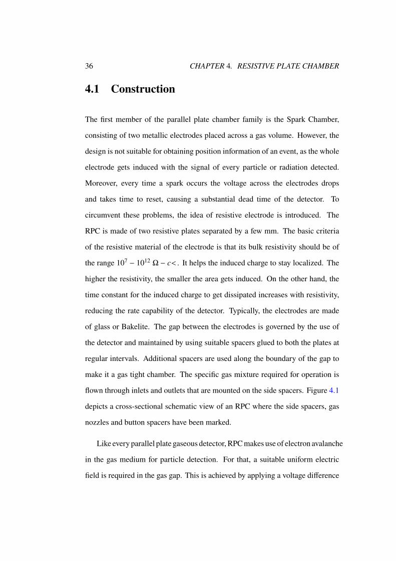
36 CHAPTER 4. RESISTIVE PLATE CHAMBER
4.1 Construction
The first member of the parallel plate chamber family is the Spark Chamber,
consisting of two metallic electrodes placed across a gas volume. However, the
design is not suitable for obtaining position information of an event, as the whole
electrode gets induced with the signal of every particle or radiation detected.
Moreover, every time a spark occurs the voltage across the electrodes drops
and takes time to reset, causing a substantial dead time of the detector. To
circumvent these problems, the idea of resistive electrode is introduced. The
RPC is made of two resistive plates separated by a few mm. The basic criteria
of the resistive material of the electrode is that its bulk resistivity should be of
the range 107 − 1012 Ω − 2<. It helps the induced charge to stay localized. The
higher the resistivity, the smaller the area gets induced. On the other hand, the
time constant for the induced charge to get dissipated increases with resistivity,
reducing the rate capability of the detector. Typically, the electrodes are made
of glass or Bakelite. The gap between the electrodes is governed by the use of
the detector and maintained by using suitable spacers glued to both the plates at
regular intervals. Additional spacers are used along the boundary of the gap to
make it a gas tight chamber. The specific gas mixture required for operation is
flown through inlets and outlets that are mounted on the side spacers. Figure 4.1
depicts a cross-sectional schematic view of an RPC where the side spacers, gas
nozzles and button spacers have been marked.
Like every parallel plate gaseous detector, RPCmakes use of electron avalanche
in the gas medium for particle detection. For that, a suitable uniform electric
field is required in the gas gap. This is achieved by applying a voltage difference
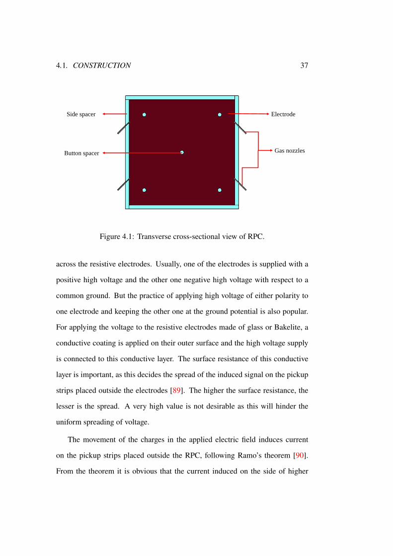
4.1. CONSTRUCTION 37
Side spacer Electrode
Gas nozzlesButton spacer
Figure 4.1: Transverse cross-sectional view of RPC.
across the resistive electrodes. Usually, one of the electrodes is supplied with a
positive high voltage and the other one negative high voltage with respect to a
common ground. But the practice of applying high voltage of either polarity to
one electrode and keeping the other one at the ground potential is also popular.
For applying the voltage to the resistive electrodes made of glass or Bakelite, a
conductive coating is applied on their outer surface and the high voltage supply
is connected to this conductive layer. The surface resistance of this conductive
layer is important, as this decides the spread of the induced signal on the pickup
strips placed outside the electrodes [89]. The higher the surface resistance, the
lesser is the spread. A very high value is not desirable as this will hinder the
uniform spreading of voltage.
The movement of the charges in the applied electric field induces current
on the pickup strips placed outside the RPC, following Ramo’s theorem [90].
From the theorem it is obvious that the current induced on the side of higher
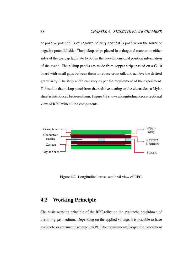
38 CHAPTER 4. RESISTIVE PLATE CHAMBER
or positive potential is of negative polarity and that is positive on the lower or
negative potential side. The pickup strips placed in orthogonal manner on either
sides of the gas gap facilitate to obtain the two-dimensional position information
of the event. The pickup panels are made from copper strips pasted on a G-10
board with small gaps between them to reduce cross talk and achieve the desired
granularity. The strip width can vary as per the requirement of the experiment.
To insulate the pickup panel from the resistive coating on the electrodes, a Mylar
sheet is introduced between them. Figure 4.2 shows a longitudinal cross-sectional
view of RPC with all the components.
Pickup board Copper
StripConductive
coating Resistive
ElectrodesGas gap
SpacersMylar Sheet
Figure 4.2: Longitudinal cross-sectional view of RPC.
4.2 Working Principle
The basic working principle of the RPC relies on the avalanche breakdown of
the filling gas medium. Depending on the applied voltage, it is possible to have
avalanche or streamer discharge in RPC. The requirement of a specific experiment
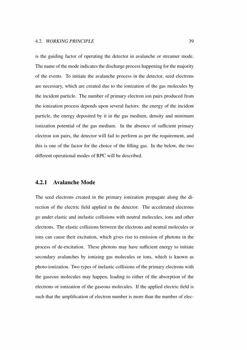
4.2. WORKING PRINCIPLE 39
is the guiding factor of operating the detector in avalanche or streamer mode.
The name of the mode indicates the discharge process happening for the majority
of the events. To initiate the avalanche process in the detector, seed electrons
are necessary, which are created due to the ionization of the gas molecules by
the incident particle. The number of primary electron ion pairs produced from
the ionization process depends upon several factors: the energy of the incident
particle, the energy deposited by it in the gas medium, density and minimum
ionization potential of the gas medium. In the absence of sufficient primary
electron ion pairs, the detector will fail to perform as per the requirement, and
this is one of the factor for the choice of the filling gas. In the below, the two
different operational modes of RPC will be described.
4.2.1 Avalanche Mode
The seed electrons created in the primary ionization propagate along the di-
rection of the electric field applied in the detector. The accelerated electrons
go under elastic and inelastic collisions with neutral molecules, ions and other
electrons. The elastic collisions between the electrons and neutral molecules or
ions can cause their excitation, which gives rise to emission of photons in the
process of de-excitation. These photons may have sufficient energy to initiate
secondary avalanches by ionizing gas molecules or ions, which is known as
photo-ionization. Two types of inelastic collisions of the primary electrons with
the gaseous molecules may happen, leading to either of the absorption of the
electrons or ionization of the gaseous molecules. If the applied electric field is
such that the amplification of electron number is more than the number of elec-
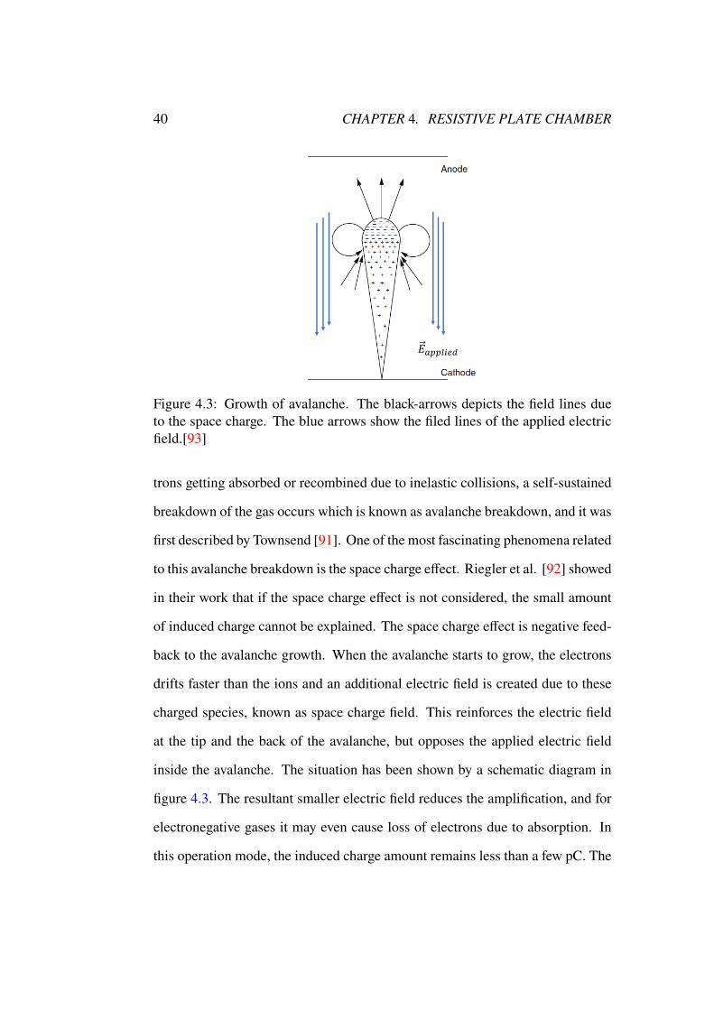
40 CHAPTER 4. RESISTIVE PLATE CHAMBER
𝐸𝑎𝑝𝑝𝑙𝑖𝑒𝑑
Figure 4.3: Growth of avalanche. The black-arrows depicts the field lines dueto the space charge. The blue arrows show the filed lines of the applied electricfield.[93]
trons getting absorbed or recombined due to inelastic collisions, a self-sustained
breakdown of the gas occurs which is known as avalanche breakdown, and it was
first described by Townsend [91]. One of the most fascinating phenomena related
to this avalanche breakdown is the space charge effect. Riegler et al. [92] showed
in their work that if the space charge effect is not considered, the small amount
of induced charge cannot be explained. The space charge effect is negative feed-
back to the avalanche growth. When the avalanche starts to grow, the electrons
drifts faster than the ions and an additional electric field is created due to these
charged species, known as space charge field. This reinforces the electric field
at the tip and the back of the avalanche, but opposes the applied electric field
inside the avalanche. The situation has been shown by a schematic diagram in
figure 4.3. The resultant smaller electric field reduces the amplification, and for
electronegative gases it may even cause loss of electrons due to absorption. In
this operation mode, the induced charge amount remains less than a few pC. The

4.2. WORKING PRINCIPLE 41
avalanche mode of operation has the following advantages and disadvantages.
• In case of small amount, charge is induced. Smaller the amount of charge
less the number of induced copper strips. In case of ICAL the charge
profile is not available. So, less the number of hit strips, more accurate
will be the position determination and better spatial resolution.
• The typical time resolution achieved for this mode is around 1 ns.
• It takes a small amount of time for the little amount of charges to get
dissipated, which makes this operation mode capable of handling high
event rate.
• The small induced charge requires state of the art electronic system to
process the signal. Without a dedicated pre-amplifier, it becomes difficult
to identify the signal.
4.2.2 Streamer mode
This mode of operation takes place at higher electric field than the previous one.
As the name suggests, in this mode the streamer discharge occurs for most of the
events. When the electron avalanche starts growing under its own space charge
field rather than the applied one, it is known as streamer discharge. Depending
upon the growth mechanism, the streamer discharge can be classified as follows
• Positive Streamer or Cathode Directed Streamer
• Negative Streamer or Anode Directed Streamer.

42 CHAPTER 4. RESISTIVE PLATE CHAMBER
Figure 4.4: Schematic diagram of positive streamer formation [93].
4.2.2.1 Positive Streamer or Cathode Directed Streamer
Streamer discharge starts with an avalanche as shown in figure 4.4 (a) with the
electrons moving faster than the ions. The drift velocity of ions is usually 3
orders of magnitude smaller than that of the electrons. As a result, by the time
the avalanche reaches to the anode and starts losing electrons, the ions can not
reach to the cathode, which is shown in figure 4.4 (b). At this point, the space
charge field of the ions comes into play. If the number of the ions is so large
that the space charge field is equal to that of the applied one, it starts attracting
all the secondary avalanches towards it as shown in figure 4.4 (c). The electrons
of these secondary avalanches upon reaching the zone with high density of ions
recombine with some ions present there, leaving back their ions, which shifts the
high density ion zone towards the cathode. Just behind this zone, a quasi neutral
plasma of electrons and ions is created, as shown in figure 4.4 (c). The shifted
high density ion zone again attracts other secondary avalanches and in the same
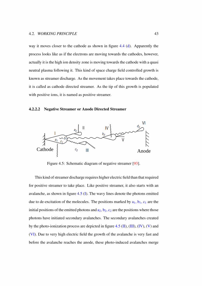
4.2. WORKING PRINCIPLE 43
way it moves closer to the cathode as shown in figure 4.4 (d). Apparently the
process looks like as if the electrons are moving towards the cathodes, however,
actually it is the high ion density zone is moving towards the cathode with a quasi
neutral plasma following it. This kind of space charge field controlled growth is
known as streamer discharge. As the movement takes place towards the cathode,
it is called as cathode directed streamer. As the tip of this growth is populated
with positive ions, it is named as positive streamer.
4.2.2.2 Negative Streamer or Anode Directed Streamer
Cathode Anode
Figure 4.5: Schematic diagram of negative streamer [93].
This kind of streamer discharge requires higher electric field than that required
for positive streamer to take place. Like positive streamer, it also starts with an
avalanche, as shown in figure 4.5 (I). The wavy lines denote the photons emitted
due to de-excitation of the molecules. The positions marked by a1, b1, c1 are the
initial positions of the emitted photons and a2, b2, c2 are the positions where those
photons have initiated secondary avalanches. The secondary avalanches created
by the photo-ionization process are depicted in figure 4.5 (II), (III), (IV), (V) and
(VI). Due to very high electric field the growth of the avalanche is very fast and
before the avalanche reaches the anode, these photo-induced avalanches merge

44 CHAPTER 4. RESISTIVE PLATE CHAMBER
into it. The space charge field of the combined avalanches becomes equal to the
applied field and keeps on growing towards the anode. In this discharge case,
the tip of the avalanche is populated with electrons and so named as negative
streamer. As the growth takes place towards the anode, it is known as anode
directed streamer.
Like the avalanche mode of operation, the streamer mode has its own merits
and demerits, as the following.
• The large amount of induced charges rules out the necessity of pre-
amplification.
• The large amount of charges takes a longer time to dissipate and increases
the dead time and hence reduces the rate capability.
• The streamer pulse has an avalanche pre-cursor. Moreover, the time gap
between the avalanche pre-cursor and the streamer pulse is not fixed, which
worsens the time resolution. Sometimes an after pulse can be observed,
which also affects the time resolution.
• The large amount of charges gets induced to more number of strips and the
spatial information gets diluted.
In the next chapter a numerical method will be introduced which has been
devised to emulate the dynamics of the charges taking place in the RPC as
described in this chapter.

Chapter 5Numerical Modelling of RPC
In the previous chapter, the structure and working principle of RPC have been
described briefly. Owing to its design, an RPC can operate in two modes,
avalanche and streamer, depending upon the requirements of the experiments.
The flexibility in its design can offer excellent time resolution (few hundreds
of picosecond) and very good spatial resolution (few hundreds of micrometer)
as well. As a result, the RPC is widely used for both tracking and triggering
purposes in high energy physics (HEP) experiments. Such a diverse use of
this detector has prompted the HEP community to use numerical simulation as
another tool to understand its mechanism in order to predict its performance in
various experiments or interpret and analyze the observed data. Many attempts
have been made to simulate the avalanche and streamer modes of functioning of
RPC. Most of them are based on either Monte Carlo methods [92, 94, 95, 96,
97] or hydrodynamic approach [98, 99, 100]. A review of different simulation
methods can be found here [101].
In this chapter, a numerical model will be first described which has been built
45
46 CHAPTER 5. NUMERICAL MODELLING OF RPC
on the basis of hydrodynamic model of electronic and ionic transports to simulate
the streamer and avalanche modes of RPC. It studies the growth and propagation
of the charges in an RPC produced due to incident cosmic muons at different
applied voltages. The entire framework has been developed on the platform of
a commercial Finite Element Method (FEM) package, COMSOL Multiphysics
[102]. It has utilized relevant information of primary ionization produced by a
package HEED [103], and electron transport parameters in the gaseous medium
produced by another package MAGBOLTZ [104] that are required to carry out
the simulation. The procedure to calculate efficiency and streamer probability
of the RPC operated with a given gas mixture using this numerical model will
be described next. The results will be compared to the experimental data [105,
106, 107] available for several R134a-based gas mixtures in order to validate the
numerical model.
In section 5.1 the numericalmodelwill be described. The next section 5.2will
be dedicated to the discussion of the avalanche and streamer discharge simulations
using the model. The next section 5.3 present a procedure of calculating a few
detector responses, such as the streamer probability and efficiency, using the
simulation. Following this, in section 5.4 the simulated efficiency and streamer
probabilities will be comparedwith experimental measurements reported in [105,
106, 107].
5.1 Numerical Modelling
The present numerical model has considered the gas mixture as a charged solu-
tion. It assumes the neutral gas molecules as the solvent and all the charge species
5.1. NUMERICAL MODELLING 47
(electrons and ions) produced in the medium due to ionization as well as photo-
ionization as solutes. In the following section 5.1.1, the geometry of the RPC
that has been considered in the simulation will be described. In the next section
5.1.2, the mathematical model following the hydrodynamics adopted to carry out
the simulation will be discussed. The conditions to identify the avalanche and
streamer modes of operation will be mentioned in the section 5.1.3.
5.1.1 Model Geometry
3D modelling of an RPC would obviously be the best choice for simulating
the charge dynamics in the device. However, it has not been attempted in the
present study as it involves extensive computational expenses. Both of the 2D
Cartesian and axisymmetricmodelling approaches have their own advantages and
limitations. In the Cartesian modelling, the charge growth is simulated in the 2D
transverse cross-section (XZ-plane) of the detector active volume. On the other
hand, the axisymmetric model simulates the growth on one side of the Z-axis
and imposes rotational symmetry to achieve an approximate 3D representation of
the physical processes at lower computational expenditure. In the present work,
the 2D Cartesian model has been implemented to achieve the two-dimensional
growth of the avalanche.
The RPC model has a gas gap (along Z-direction) of 2 mm, as illustrated
in figure 5.1. The electric field has been applied across the gas gap along the
positive Z-direction. The length of the RPC has been considered 1mmonly in the
X-direction because the maximum radius of avalanche or streamer never exceeds1U[91], where U is the first Townsend coefficient. It is of the order of 10 mm−1 for
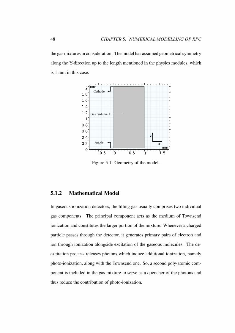
48 CHAPTER 5. NUMERICAL MODELLING OF RPC
the gasmixtures in consideration. Themodel has assumed geometrical symmetry
along the Y-direction up to the length mentioned in the physics modules, which
is 1 mm in this case.
Cathode
Anode
Gas Volume
Figure 5.1: Geometry of the model.
5.1.2 Mathematical Model
In gaseous ionization detectors, the filling gas usually comprises two individual
gas components. The principal component acts as the medium of Townsend
ionization and constitutes the larger portion of the mixture. Whenever a charged
particle passes through the detector, it generates primary pairs of electron and
ion through ionization alongside excitation of the gaseous molecules. The de-
excitation process releases photons which induce additional ionization, namely
photo-ionization, along with the Townsend one. So, a second poly-atomic com-
ponent is included in the gas mixture to serve as a quencher of the photons and
thus reduce the contribution of photo-ionization.
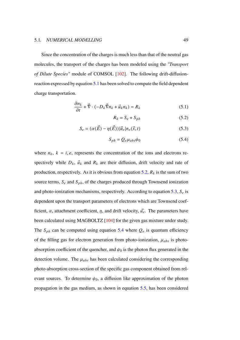
5.1. NUMERICAL MODELLING 49
Since the concentration of the charges is much less than that of the neutral gas
molecules, the transport of the charges has been modeled using the "Transport
of Dilute Species" module of COMSOL [102]. The following drift-diffusion-
reaction expressed by equation 5.1 has been solved to compute the field dependent
charge transportation.
m=:
mC+ ®∇ · (−�:
®∇=: + ®D:=: ) = ': (5.1)
': = (4 + (?ℎ (5.2)
(4 = (U( ®�) − [( ®�)) | ®D4 |=4 (®G, C) (5.3)
(?ℎ = &4`01Bk0 (5.4)
where =: , : = 8, 4, represents the concentration of the ions and electrons re-
spectively while �: , ®D: and ': are their diffusion, drift velocity and rate of
production, respectively. As it is obvious from equation 5.2, ': is the sum of two
source terms, (4 and (?ℎ, of the charges produced through Townsend ionization
and photo-ionization mechanisms, respectively. According to equation 5.3, (4 is
dependent upon the transport parameters of electrons which are Townsend coef-
ficient, U, attachment coefficient, [, and drift velocity, ®D4. The parameters have
been calculated using MAGBOLTZ [104] for the given gas mixture under study.
The (?ℎ can be computed using equation 5.4 where &4 is quantum efficiency
of the filling gas for electron generation from photo-ionization, `01B is photo-
absorption coefficient of the quencher, and k0 is the photon flux generated in the
detection volume. The `01B has been calculated considering the corresponding
photo-absorption cross-section of the specific gas component obtained from rel-
evant sources. To determine k0, a diffusion like approximation of the photon
propagation in the gas medium, as shown in equation 5.5, has been considered
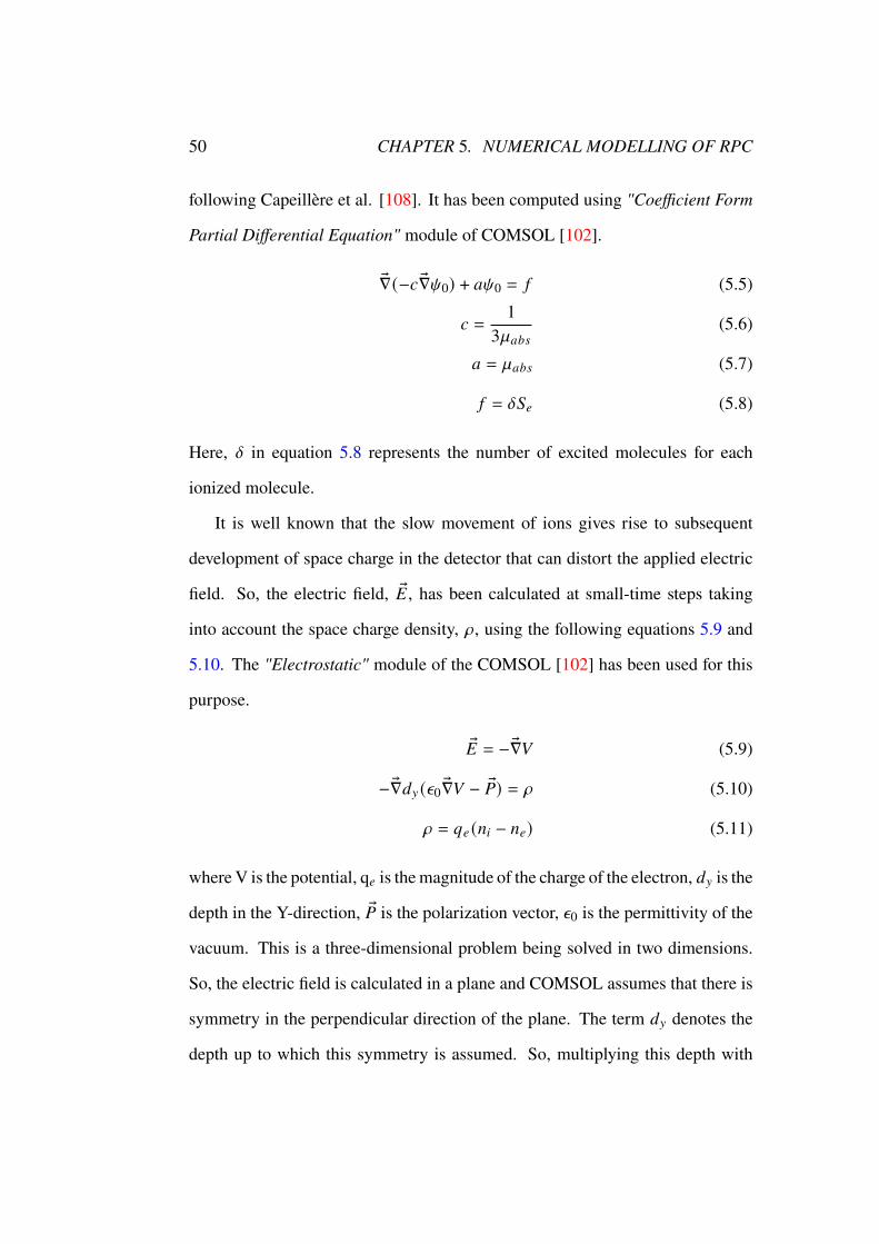
50 CHAPTER 5. NUMERICAL MODELLING OF RPC
following Capeillère et al. [108]. It has been computed using "Coefficient Form
Partial Differential Equation" module of COMSOL [102].
®∇(−2 ®∇k0) + 0k0 = 5 (5.5)
2 =1
3`01B(5.6)
0 = `01B (5.7)
5 = X(4 (5.8)
Here, X in equation 5.8 represents the number of excited molecules for each
ionized molecule.
It is well known that the slow movement of ions gives rise to subsequent
development of space charge in the detector that can distort the applied electric
field. So, the electric field, ®� , has been calculated at small-time steps taking
into account the space charge density, d, using the following equations 5.9 and
5.10. The "Electrostatic" module of the COMSOL [102] has been used for this
purpose.
®� = −®∇+ (5.9)
−®∇3H (n0 ®∇+ − ®%) = d (5.10)
d = @4 (=8 − =4) (5.11)
where V is the potential, q4 is themagnitude of the charge of the electron, 3H is the
depth in the Y-direction, ®% is the polarization vector, n0 is the permittivity of the
vacuum. This is a three-dimensional problem being solved in two dimensions.
So, the electric field is calculated in a plane and COMSOL assumes that there is
symmetry in the perpendicular direction of the plane. The term 3H denotes the
depth up to which this symmetry is assumed. So, multiplying this depth with
5.1. NUMERICAL MODELLING 51
the amount of charge in a plane gives the total amount of charge in the volume
with the depth 3H. The change of electric field has been considered in the X and
Z-directions, while it has been considered constant in the Y-direction.
The following boundary conditions have been used in the model. The loss
of electrons from the gas gap upon reaching the anode has been taken care of
by assuming drift of the electrons through the anode. Similar condition has
been set about the ions to consider their outflow at the cathode. To incorporate
the processes of electrons and ions diffusing and drifting out of the simulated
volume, the two boundaries other than the cathode and the anode have been
assumed open for them. The photon flux at the electrodes has been taken as zero,
as these electrodes are made up of those materials which do not have scintillating
property. This condition has been implemented as a Dirichlet boundary condition
in the model. The photon propagation out of the simulation volume has been
taken into account by considering the two boundaries other than the electrodes
open for them.
5.1.3 Conditions for Avalanche and Streamer
The main characteristic of streamer is that the electric field due to space charge
equals the applied electric field [93, 91]. On the other hand, in case of avalanche,
the number of electrons becomes zero due to their loss upon reaching the anode.
These two conditions have been utilized to identify the streamer and avalanche
and subsequently stop the simulation. The aforementioned conditions have been
implemented in the following way:
• Avalanche: All the electrons have been collected in the anode.

52 CHAPTER 5. NUMERICAL MODELLING OF RPC
• Streamer: When the space charge field has become equal to the applied
field (W = 1) where W = (�C>C0; − �0??;843)/�0??;843 is a parameter for
comparing the space charge field to the actual applied one.
5.2 Simulated Avalanche and Streamer Discharge
Figure 5.2 and 5.3 are typical examples of avalanche and streamer events, re-
spectively, where the evolution of the electron density with time in the gas gap
for both the conditions have been depicted. The color code represents the natural
logarithm of the electron density in the gas gap. The boundary for each time slice
denotes the boundary of the model geometry. In figure 5.3, the movement of the
higher electron density region towards the cathode can be seen, as is observed
experimentally in case of positive streamers.
Cathode
Anode
ln(Electron density (1/m3))
(Z = 2 mm)
(Z = 0 mm)X
Z0 mm 1 mm
Figure 5.2: Growth of electronic charges in RPC for avalanche at 41 kV/cm for10 primary electrons with mean Z-position of 1.2 mm
In figure 5.4, time evolution of the electric field and electron density for the
streamer condition at applied field 47 kV/cm is shown. The background solid
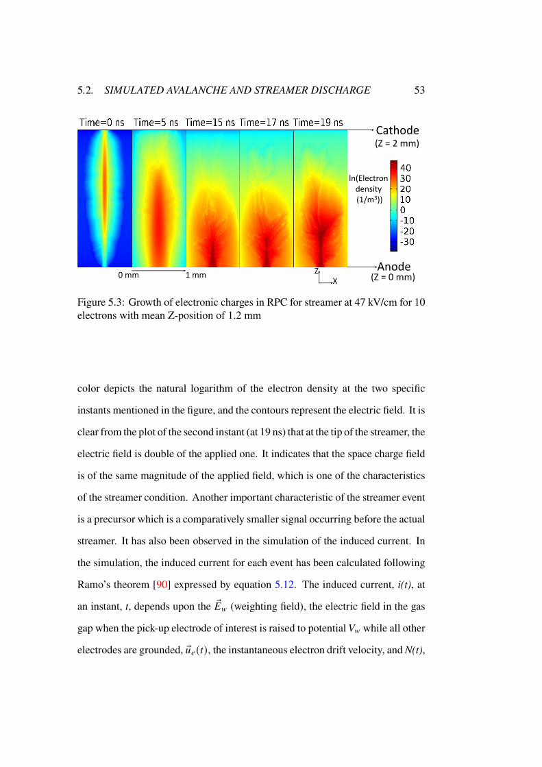
5.2. SIMULATED AVALANCHE AND STREAMER DISCHARGE 53
Cathode
Anode
ln(Electrondensity(1/m3))
(Z = 2 mm)
(Z = 0 mm)XZ0 mm 1 mm
Figure 5.3: Growth of electronic charges in RPC for streamer at 47 kV/cm for 10electrons with mean Z-position of 1.2 mm
color depicts the natural logarithm of the electron density at the two specific
instants mentioned in the figure, and the contours represent the electric field. It is
clear from the plot of the second instant (at 19 ns) that at the tip of the streamer, the
electric field is double of the applied one. It indicates that the space charge field
is of the same magnitude of the applied field, which is one of the characteristics
of the streamer condition. Another important characteristic of the streamer event
is a precursor which is a comparatively smaller signal occurring before the actual
streamer. It has also been observed in the simulation of the induced current. In
the simulation, the induced current for each event has been calculated following
Ramo’s theorem [90] expressed by equation 5.12. The induced current, i(t), at
an instant, t, depends upon the ®�F (weighting field), the electric field in the gas
gap when the pick-up electrode of interest is raised to potential+F while all other
electrodes are grounded, ®D4 (C), the instantaneous electron drift velocity, andN(t),
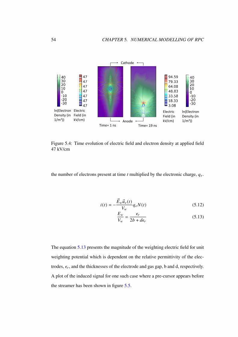
54 CHAPTER 5. NUMERICAL MODELLING OF RPC
Time= 19 ns
Electric Field (in kV/cm)
ln(Electron Density (in 1/m3))
Electric Field (in kV/cm)
ln(Electron Density (in 1/m3))
Time= 1 ns
Cathode
Anode
Figure 5.4: Time evolution of electric field and electron density at applied field47 kV/cm
the number of electrons present at time t multiplied by the electronic charge, @4.
8(C) = −®�F ®D4 (C)+F
@4# (C) (5.12)
�F
+F=
nA
21 + 3nA(5.13)
The equation 5.13 presents the magnitude of the weighting electric field for unit
weighting potential which is dependent on the relative permittivity of the elec-
trodes, nA , and the thicknesses of the electrode and gas gap, b and d, respectively.
A plot of the induced signal for one such case where a pre-cursor appears before
the streamer has been shown in figure 5.5.

5.3. CALCULATION OF STREAMER PROBABILITY AND EFFICIENCY 55
-3
-2.5
-2
-1.5
-1
-0.5
0
0 2 4 6 8 10 12 14 16 18 20
Cu
rren
t (m
A)
Time (ns)
Precursor
Streamer
Figure 5.5: Induced current in case of a streamer event at 47 kV/cm
5.3 Calculation of Streamer Probability and
Efficiency
A method of calculating the detector responses of streamer probability and the
efficiency at different applied voltages, which are considered as figures of merit
of RPC operation, for the given gas using the numerical model will be described
in this section. For validation of the calculation procedure, the results will be
compared with experimental data presented in several references [105, 106, 107].
Two gas mixtures have been considered for the calculation. One of them is a
mixture of R134a(95%):n-C4H10(5%) [105] and the other is the usual one of
R134a(95.2%):i-C4H10(4.5%):SF6(0.3%) [106, 107] which will be used in the
RPCs of the ICALwith same volumetric percentages. In this work, 1 bar pressure
56 CHAPTER 5. NUMERICAL MODELLING OF RPC
and 293.15 K temperature have been maintained throughout the calculation.
5.3.1 Event Generation
In the simulation, a flux of 10,000 cosmic muons with energy between 1 - 10
GeV have been considered for event generation in the RPC. As the efficiency and
streamer probability of the detector are independent of the direction of incidence
of the charged particle, for brevity only those muons falling within zenith angle
0◦ - 13◦ have been considered. Eventually, the cosmic muon flux given by Tang et
al. [109] has been followed and HEED has been used to compute the number of
primary electrons generated in the gas gap due to ionization caused by thesemuon
events. For each muon event, it has provided the number of primary clusters,
their position and number of electrons lying in each cluster. It has been found
that the clusters are distributed throughout the whole gas gap and in most cases
contain one electron. Instead of carrying out the simulation of the growth of each
cluster produced in a muon event, those have been collectively represented as a
single cluster with its Z-position and size (number of electrons in it) calculated
from this information of each cluster as provided by the HEED in the following
way. The Z-position of the representative cluster for an event has been obtained
from the weighted mean of the same of all the primary clusters and its size
from the sum of all the primary electrons created in that event. Further, these
events with representative seed clusters having similar size and mean Z-positions
falling within a specified range have been considered as a group. Eventually,
the simulation of charge growth following hydrodynamics has been carried out
for a single seed cluster has belonging to the group of events. This approach of
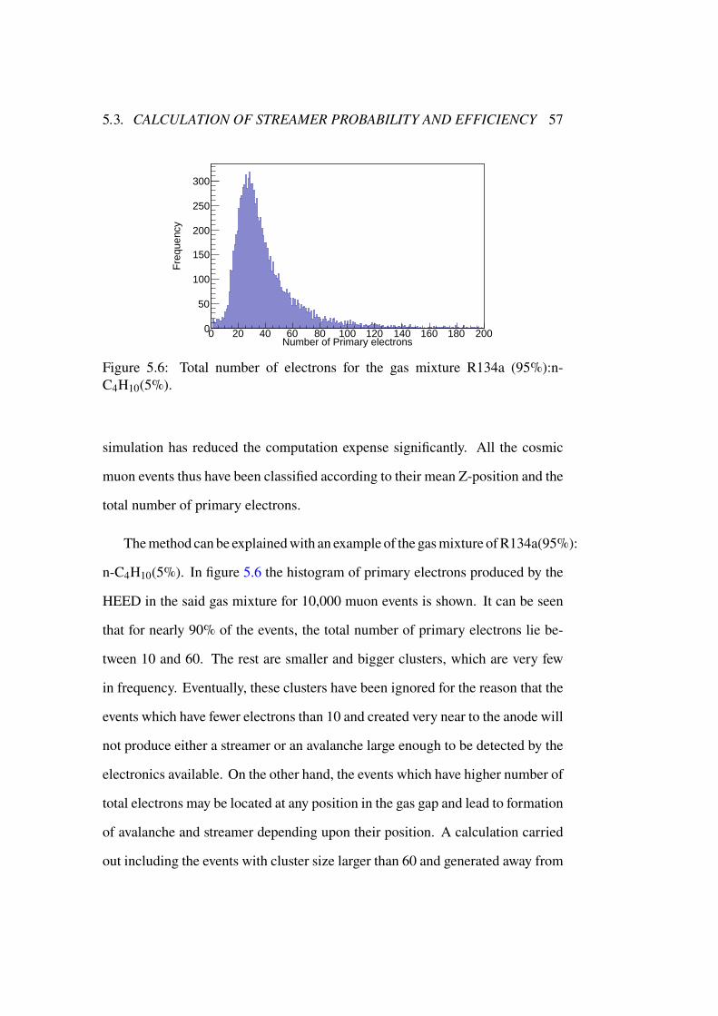
5.3. CALCULATION OF STREAMER PROBABILITY AND EFFICIENCY 57
0 20 40 60 80 100 120 140 160 180 200Number of Primary electrons
0
50
100
150
200
250
300F
requ
ency
Figure 5.6: Total number of electrons for the gas mixture R134a (95%):n-C4H10(5%).
simulation has reduced the computation expense significantly. All the cosmic
muon events thus have been classified according to their mean Z-position and the
total number of primary electrons.
Themethod can be explainedwith an example of the gasmixture ofR134a(95%):
n-C4H10(5%). In figure 5.6 the histogram of primary electrons produced by the
HEED in the said gas mixture for 10,000 muon events is shown. It can be seen
that for nearly 90% of the events, the total number of primary electrons lie be-
tween 10 and 60. The rest are smaller and bigger clusters, which are very few
in frequency. Eventually, these clusters have been ignored for the reason that the
events which have fewer electrons than 10 and created very near to the anode will
not produce either a streamer or an avalanche large enough to be detected by the
electronics available. On the other hand, the events which have higher number of
total electrons may be located at any position in the gas gap and lead to formation
of avalanche and streamer depending upon their position. A calculation carried
out including the events with cluster size larger than 60 and generated away from
58 CHAPTER 5. NUMERICAL MODELLING OF RPC
the anode has demonstrated an increase in the computational time without af-
fecting the result much. Therefore, to save the computational expenditure at the
cost of marginal error, these events have been opted out of the calculation. For
the rest 90% of total 10,000 muon events, the seed clusters have been produced
for each case and further grouped following a range of 0.1 mm in their mean
Z-position and 5 in the cluster size. Figure 5.7 depicts a 2D histogram of the size
and mean Z-position of the seed clusters for the 90% muon events considered in
the simulation for the gas mixture of R134a (95%):n-C4H10 (5%). It shows the
distribution of the seed clusters according to their mean Z-position binned with
a bin size of 0.1 mm over a range of 0.1 - 1.9 mm and the number of primary
electrons with a bin size of 5 over a range of 10 - 60. The frequency for each
2D cell has been written there, which denotes the number of events having seed
clusters with mean Z-position and size falling within the range of the respective
cell. For each cell, the hydrodynamic simulation has been carried out considering
the minimum mean Z-position and size of the respective cell. Depending upon
the charge evolution simulated by the model with the said Z-position and size,
all the events belonging to the cell have been classified as avalanche or streamer
events. The same 2D histogram for the gas mixture of R134a (95.2%): i-C4H10
(4.5%): SF6 (0.3%) has been illustrated in figure 5.8 which has been produced
following the method described above.
The seed cluster has been represented by a Gaussian distribution [98] with its
mean position same as the mean Z-position considered for the respective group of
events. As the simulation has considered a 2Dmodel of the RPC in the XZ-plane,
a two variable Gaussian distribution has been used. The standard deviation for
the Z-variable of the Gaussian has been kept fixed for each seed cluster, with the

5.3. CALCULATION OF STREAMER PROBABILITY AND EFFICIENCY 59
1 5 12 14 16 17 46 54 66 71 48 36 16 2 1
3 7 9 7 24 49 109
162
213
199
151
80 41 15 2 1
2 2 5 12 16 56 131
244
358
317
229
125 51 14 4 1
1 2 4 29 60 138
229
329
315
255
131
55 20 2 1
1 1 9 11 50 110
179
250
248
174
109 39 21 5 1
1 2 3 8 21 46 76 129
165
168
132 71 49 12 4 1
1 1 7 17 43 62 94 92 85 95 61 34 19 10 1 1
1 1 1 10 22 43 64 61 59 64 70 53 26 16 7 5
2 15 21 25 43 38 51 52 29 35 31 18 5 4 1
1 3 10 18 23 30 40 26 41 31 24 17 23 5 4
0.2 0.4 0.6 0.8 1 1.2 1.4 1.6 1.8Mean Z position (in mm)
10
15
20
25
30
35
40
45
50
55
60N
umbe
r of
prim
ary
elec
tron
s
Figure 5.7: 2D histogram of muon events for the gas mixture of R134a (95%):n-C4H10 (5%).
condition that the 5f of the distribution always remains bound by the electrodes.
As mostly vertical muon events have been considered, the mean of the X-variable
of the Gaussian has been considered to be 0.5 mm, which is at the middle of the
model geometry.
5.3.2 Estimation of Detector Responses
It is obvious from the discussion in section 5.3.1 that for each of the 10,000
muon events, a seed cluster having definite size and mean Z-position could be
prepared to initiate the hydrodynamic simulation of detector response for a given
voltage configuration. From the numerical study, a correlation of the occurrence
of avalanche or streamer at an applied voltage to the size and the position of the
seed cluster has been observed. Therefore, the avalanche and streamer modes
are viable to be distinguished on the basis of these two parameters. Once the
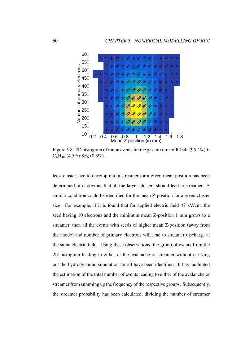
60 CHAPTER 5. NUMERICAL MODELLING OF RPC
2 6 17 47 62 80 80 58 29 16 5 1
3 8 52 96 170
232
229
175 86 29 17 1
5 13 51 134
273
342
352
254
130 57 14 8 1
2 20 63 125
241
363
356
251
127 61 16 7 1
1 3 19 53 102
173
269
265
201
119 49 24 11 1
3 2 21 37 88 111
138
192
150 76 40 13 4 5
1 12 17 43 59 92 116
118 80 67 37 15 9 2 2
1 4 5 21 29 52 59 78 67 62 50 34 24 8 2 1
11 19 35 29 54 27 37 45 37 33 9 10 4 1
1 6 15 15 20 32 32 30 29 27 22 8 10 3 1
0.2 0.4 0.6 0.8 1 1.2 1.4 1.6 1.8Mean Z position (in mm)
10
15
20
25
30
35
40
45
50
55
60
Num
ber
of p
rimar
y el
ectr
ons
Figure 5.8: 2D histogram of muon events for the gas mixture of R134a (95.2%):i-C4H10 (4.5%):SF6 (0.3%).
least cluster size to develop into a streamer for a given mean position has been
determined, it is obvious that all the larger clusters should lead to streamer. A
similar condition could be identified for the mean Z-position for a given cluster
size. For example, if it is found that for applied electric field 47 kV/cm, the
seed having 10 electrons and the minimum mean Z-position 1 mm grows to a
streamer, then all the events with seeds of higher mean Z-position (away from
the anode) and number of primary electrons will lead to streamer discharge at
the same electric field. Using these observations, the group of events from the
2D histogram leading to either of the avalanche or streamer without carrying
out the hydrodynamic simulation for all have been identified. It has facilitated
the estimation of the total number of events leading to either of the avalanche or
streamer from summing up the frequency of the respective groups. Subsequently,
the streamer probability has been calculated, dividing the number of streamer
5.4. VALIDATION OF NUMERICAL MODEL 61
events by the total number of muon events.
Calculation of the detector efficiency has been done in similar manner. For
this purpose, the current signal produced from the growth of the seed cluster
has been determined. The procedure to calculate the induced current has been
described in section 5.2. Only those events corresponding to the seed clusters
that have produced signals crossing a predefined threshold of current, have been
considered as valid events. In experiments, a signal in terms of voltage is collected
after electronic amplification of the current signal across a load resistance. In
the simulation, this has been implemented by calculating the current equivalent
to the voltage mentioned as threshold after the electronic gain. The ratio of the
valid events with respect to the total number of events has been defined as the
detector efficiency.
5.4 Validation of Numerical Model
In this section, the aforementioned procedure of calculating streamer probability
and RPC efficiency using the 2D histogram will be validated by comparing the
results for different gas mixtures with respective experimental data. For the gas
mixture of R134a(95%):n-C4H10(5%), the comparison of the calculated values
of streamer probability and the efficiency will be compared to the experimental
observation [105] in section 5.4.1. The following section 5.4.2 will discuss the
comparison between experimental data presented in [106, 107] and simulated
streamer probability and efficiency for the gas mixture of R134a(95.2%): i-
C4H10(4.5%): SF6(0.3%).
62 CHAPTER 5. NUMERICAL MODELLING OF RPC
5.4.1 Comparison for R134a(95%):n-C4H10(5%)
For each combination of the size and mean Z-position of the seed cluster, the
evolution of the charged fluid has been simulated at different applied voltages.
Criteria discussed in section 5.1.3 have been used to determine the nature of
the RPC signal as either of avalanche or streamer. In order to compare with
the experimental measurements of efficiency and streamer probability reported
in [105], the same observable have been estimated using the present simulation
model.
A threshold criterion following a similar condition mentioned in [105] has
been used in the present calculation to select the valid signals as required to
calculate the efficiency. In [105], it has been considered that the amplitude of
the signal should be greater than 30 mV which is equivalent to 0.1 mV signal
acquired across a 25 Ω resistor with an electronic gain of 300. In the present
calculation, the current corresponding to this threshold criteria has been calcu-
lated and considered as the threshold to identify the valid events. In figure 5.9, a
comparison between the simulation and experimental data for the efficiency has
been plotted. The simulation has been carried out for two values of nA (relative
permittivity of the electrode material) as that of the resistive material of the elec-
trode can vary over the given range. The comparison of the calculated streamer
probability with the experimental observation of [105] at different voltages has
been shown in figure 5.10. It can be noted from the figures 5.9 and 5.10 that the
simulation results have followed the experimental trend quite closely, although a
quantitative agreement between them has not been achieved. One of the major
reasons may be the lack of information on actual experimental conditions, which
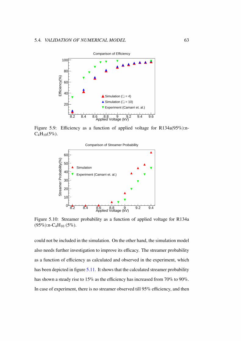
5.4. VALIDATION OF NUMERICAL MODEL 63
8.2 8.4 8.6 8.8 9 9.2 9.4 9.6 Applied Voltage (kV)
20
40
60
80
100 E
ffici
ency
(%)
Comparison of Efficiency
= 4)r∈Simulation (
= 10)r∈Simulation (
Experiment (Camarri et. al.)
Figure 5.9: Efficiency as a function of applied voltage for R134a(95%):n-C4H10(5%).
8.2 8.4 8.6 8.8 9 9.2 9.4 Applied Voltage (kV)
0
10
20
30
40
50
60
Str
eam
er P
roba
bilit
y(%
)
Comparison of Streamer Probability
Simulation
Experiment (Camarri et. al.)
Figure 5.10: Streamer probability as a function of applied voltage for R134a(95%):n-C4H10 (5%).
could not be included in the simulation. On the other hand, the simulation model
also needs further investigation to improve its efficacy. The streamer probability
as a function of efficiency as calculated and observed in the experiment, which
has been depicted in figure 5.11. It shows that the calculated streamer probability
has shown a steady rise to 15% as the efficiency has increased from 70% to 90%.
In case of experiment, there is no streamer observed till 95% efficiency, and then
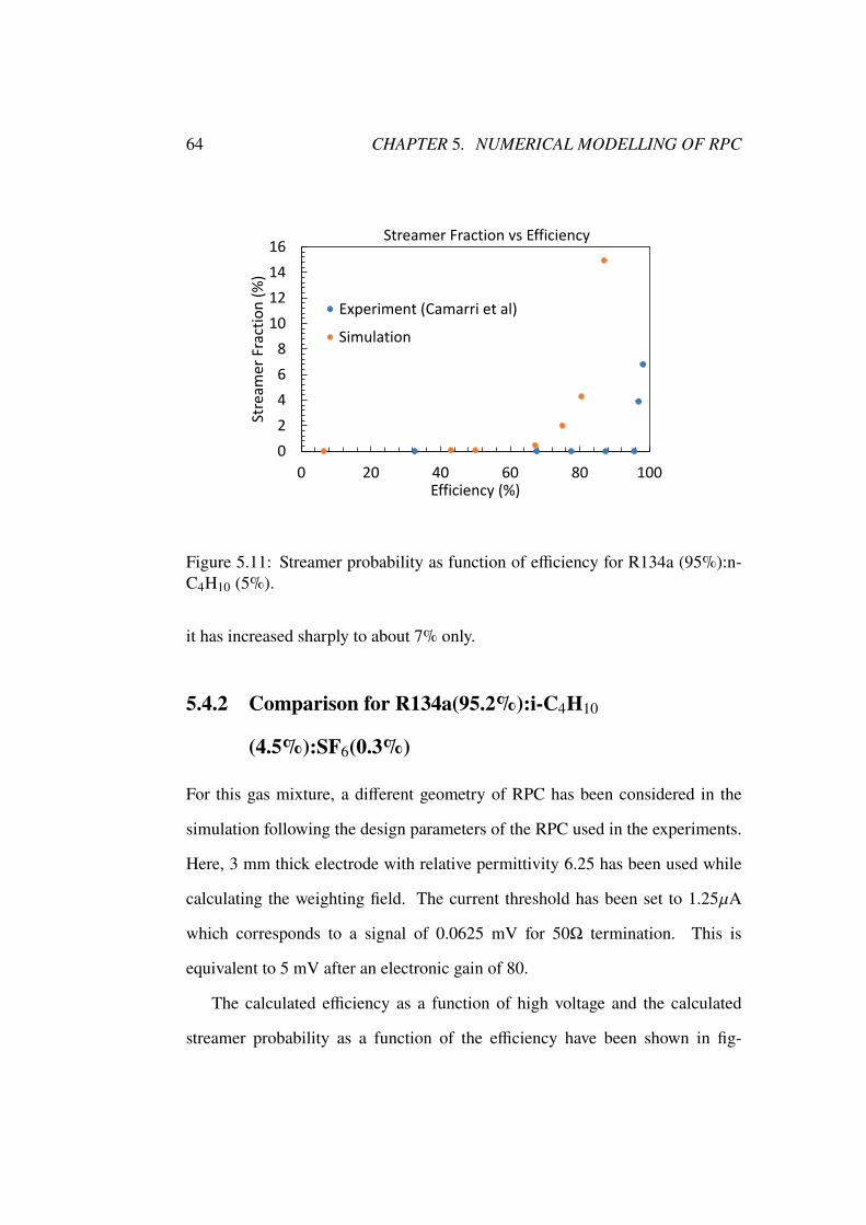
64 CHAPTER 5. NUMERICAL MODELLING OF RPC
0
2
4
6
8
10
12
14
16
0 20 40 60 80 100
Stre
amer
Fra
ctio
n (
%)
Efficiency (%)
Streamer Fraction vs Efficiency
Experiment (Camarri et al)
Simulation
Figure 5.11: Streamer probability as function of efficiency for R134a (95%):n-C4H10 (5%).
it has increased sharply to about 7% only.
5.4.2 Comparison for R134a(95.2%):i-C4H10
(4.5%):SF6(0.3%)
For this gas mixture, a different geometry of RPC has been considered in the
simulation following the design parameters of the RPC used in the experiments.
Here, 3 mm thick electrode with relative permittivity 6.25 has been used while
calculating the weighting field. The current threshold has been set to 1.25`A
which corresponds to a signal of 0.0625 mV for 50Ω termination. This is
equivalent to 5 mV after an electronic gain of 80.
The calculated efficiency as a function of high voltage and the calculated
streamer probability as a function of the efficiency have been shown in fig-
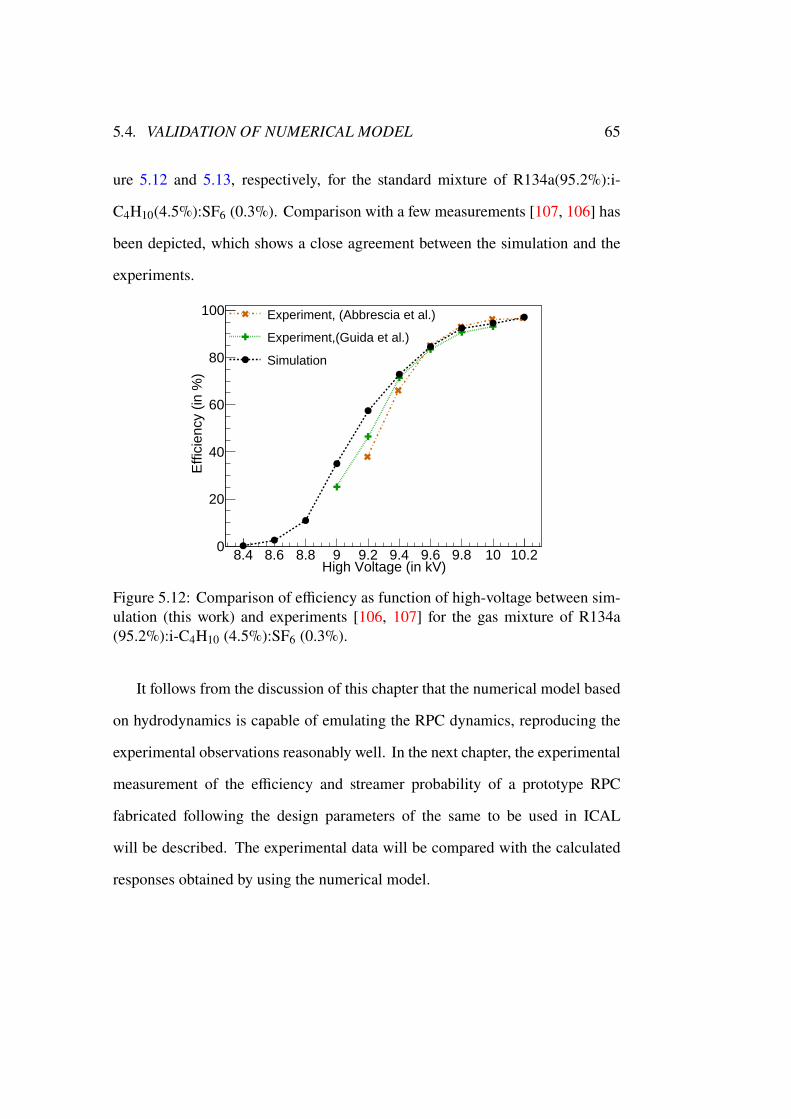
5.4. VALIDATION OF NUMERICAL MODEL 65
ure 5.12 and 5.13, respectively, for the standard mixture of R134a(95.2%):i-
C4H10(4.5%):SF6 (0.3%). Comparison with a few measurements [107, 106] has
been depicted, which shows a close agreement between the simulation and the
experiments.
8.4 8.6 8.8 9 9.2 9.4 9.6 9.8 10 10.2High Voltage (in kV)
0
20
40
60
80
100
Effi
cien
cy (
in %
)
Experiment, (Abbrescia et al.)
Experiment,(Guida et al.)
Simulation
Figure 5.12: Comparison of efficiency as function of high-voltage between sim-ulation (this work) and experiments [106, 107] for the gas mixture of R134a(95.2%):i-C4H10 (4.5%):SF6 (0.3%).
It follows from the discussion of this chapter that the numerical model based
on hydrodynamics is capable of emulating the RPC dynamics, reproducing the
experimental observations reasonably well. In the next chapter, the experimental
measurement of the efficiency and streamer probability of a prototype RPC
fabricated following the design parameters of the same to be used in ICAL
will be described. The experimental data will be compared with the calculated
responses obtained by using the numerical model.
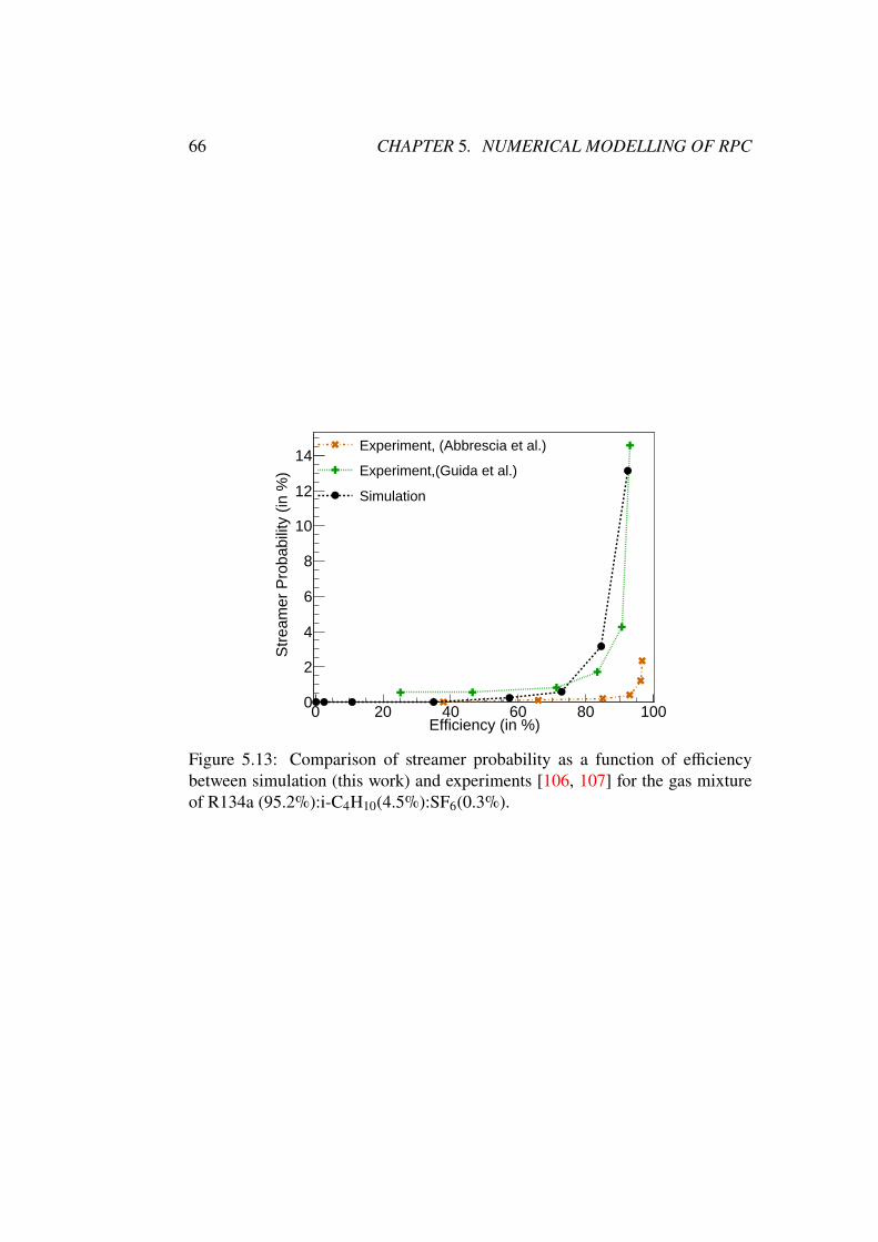
66 CHAPTER 5. NUMERICAL MODELLING OF RPC
0 20 40 60 80 100Efficiency (in %)
0
2
4
6
8
10
12
14
Str
eam
er P
roba
bilit
y (in
%)
Experiment, (Abbrescia et al.)
Experiment,(Guida et al.)
Simulation
Figure 5.13: Comparison of streamer probability as a function of efficiencybetween simulation (this work) and experiments [106, 107] for the gas mixtureof R134a (95.2%):i-C4H10(4.5%):SF6(0.3%).
Chapter 6Experimental Studies
The performance of theRPCconfigured for the ICALexperiment has been studied
by experimental measurements as well as numerical simulation to complement
each other in realizing the device dynamics. The study has also provided an
opportunity to assess the scope of the numerical model developed on the basis
of hydrodynamics in emulating the working of the RPCs of the ICAL.
The chapter has been broadly divided into three sections to discuss the ex-
perimental and numerical work and their comparison, respectively. The section
6.1 will discuss the fabrication of a prototype RPC which has been subjected to
experimental measurements of its responses. The experimental setup used for
the measurement, analysis of experimental data and the results will be described
in the following sections. The experimental result will be compared with the
numerical results as obtained in the earlier chapter 5.
67
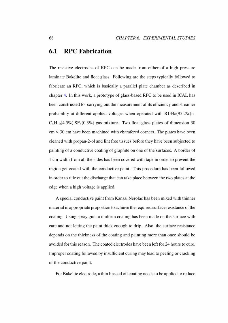
68 CHAPTER 6. EXPERIMENTAL STUDIES
6.1 RPC Fabrication
The resistive electrodes of RPC can be made from either of a high pressure
laminate Bakelite and float glass. Following are the steps typically followed to
fabricate an RPC, which is basically a parallel plate chamber as described in
chapter 4. In this work, a prototype of glass-based RPC to be used in ICAL has
been constructed for carrying out the measurement of its efficiency and streamer
probability at different applied voltages when operated with R134a(95.2%):i-
C4H10(4.5%):SF6(0.3%) gas mixture. Two float glass plates of dimension 30
cm × 30 cm have been machined with chamfered corners. The plates have been
cleaned with propan-2-ol and lint free tissues before they have been subjected to
painting of a conductive coating of graphite on one of the surfaces. A border of
1 cm width from all the sides has been covered with tape in order to prevent the
region get coated with the conductive paint. This procedure has been followed
in order to rule out the discharge that can take place between the two plates at the
edge when a high voltage is applied.
A special conductive paint from Kansai Nerolac has been mixed with thinner
material in appropriate proportion to achieve the required surface resistance of the
coating. Using spray gun, a uniform coating has been made on the surface with
care and not letting the paint thick enough to drip. Also, the surface resistance
depends on the thickness of the coating and painting more than once should be
avoided for this reason. The coated electrodes have been left for 24 hours to cure.
Improper coating followed by insufficient curing may lead to peeling or cracking
of the conductive paint.
For Bakelite electrode, a thin linseed oil coating needs to be applied to reduce
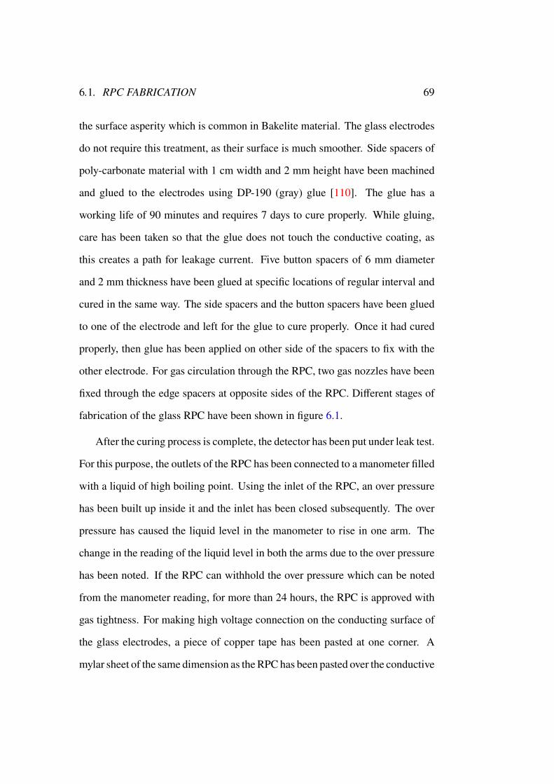
6.1. RPC FABRICATION 69
the surface asperity which is common in Bakelite material. The glass electrodes
do not require this treatment, as their surface is much smoother. Side spacers of
poly-carbonate material with 1 cm width and 2 mm height have been machined
and glued to the electrodes using DP-190 (gray) glue [110]. The glue has a
working life of 90 minutes and requires 7 days to cure properly. While gluing,
care has been taken so that the glue does not touch the conductive coating, as
this creates a path for leakage current. Five button spacers of 6 mm diameter
and 2 mm thickness have been glued at specific locations of regular interval and
cured in the same way. The side spacers and the button spacers have been glued
to one of the electrode and left for the glue to cure properly. Once it had cured
properly, then glue has been applied on other side of the spacers to fix with the
other electrode. For gas circulation through the RPC, two gas nozzles have been
fixed through the edge spacers at opposite sides of the RPC. Different stages of
fabrication of the glass RPC have been shown in figure 6.1.
After the curing process is complete, the detector has been put under leak test.
For this purpose, the outlets of the RPC has been connected to a manometer filled
with a liquid of high boiling point. Using the inlet of the RPC, an over pressure
has been built up inside it and the inlet has been closed subsequently. The over
pressure has caused the liquid level in the manometer to rise in one arm. The
change in the reading of the liquid level in both the arms due to the over pressure
has been noted. If the RPC can withhold the over pressure which can be noted
from the manometer reading, for more than 24 hours, the RPC is approved with
gas tightness. For making high voltage connection on the conducting surface of
the glass electrodes, a piece of copper tape has been pasted at one corner. A
mylar sheet of the same dimension as the RPChas been pasted over the conductive
70 CHAPTER 6. EXPERIMENTAL STUDIES
Spray painting of glass
electrodeSpacers and gas
nozzles
Surface resistivity
measurement
Leak test of RPC
A glass RPC with high voltage
connection and pickup panel
Figure 6.1: Different stages of a glass RPC fabrication.
coating to isolate the electrode from the pickup panel that have been then fixed on
the electrodes. These panels have been made of either FR4 boards or honeycomb
structure made of G-10 material with copper strips pasted on them. In this case,
the pickup panels have been made of the latter. The copper strips are 2.8 cm
wide and the gap between them is 0.2 mm. Each of the strips has been grounded
through a 50Ω resistance for impedance matching. For collecting signals from
the strips, co-axial cables of line impedance 50Ω have been connected with their
ground and that of the pickup panels connected to the common ground. For
electrical characterization of the RPC, its V-I characteristics has been studied
after flowing the gas mixture R134a(95.2%):i-C4H10(4.5%):SF6(0.3%) through
the RPC.
6.2. EXPERIMENTAL SETUP AND DATA ACQUISITION 71
6.2 Experimental Setup and Data Acquisition
The experimental setup to study the response of the glass RPC in detecting the
cosmic muons consists of and three plastic scintillator detectors in addition to the
glass RPC as shown in figure 6.2. The scintillators have been used for generating
Scintillator with PMT
Glass RPC
(a)
(b)
Figure 6.2: Experimental setup a) Side view, b) Front view.
muon triggers from their coincidence to record the data corresponding to cosmic
muon from the RPC. These scintillator detectors have been aligned with one of
the RPC pickup strips and the data have been acquired from this strip and its
two neighboring strips on either sides. The scintillator detectors are of the same
width as the RPC strip.
Biasing of the RPC has been done using CAEN A1526 module housed in
CAEN SY4527 multichannel power supply system. The power supply system
can provide up to 15 kV of voltage with current up to 1 mA. Both the positive
and negative polarity of A1526 have been used to provide high voltages to the
anode and cathode of the detector. The voltage difference over a range of 4.5 -
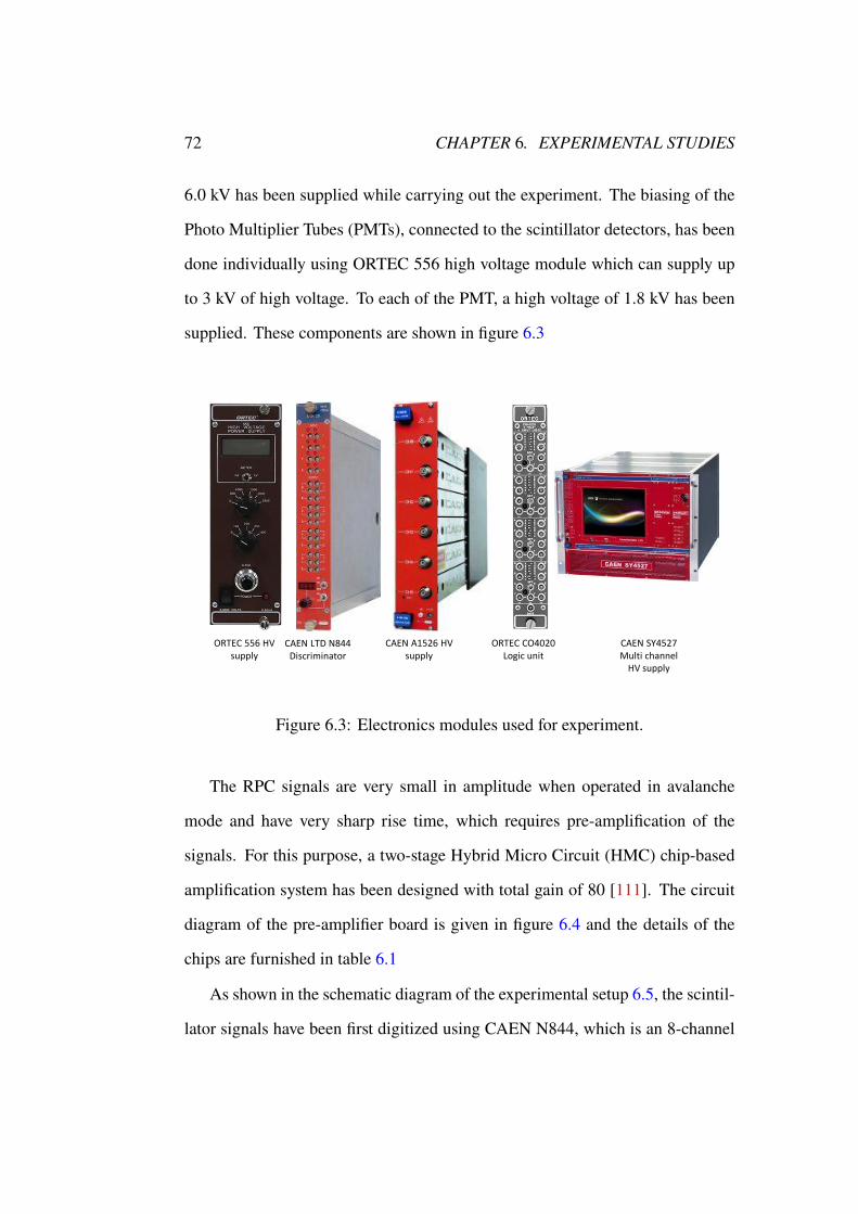
72 CHAPTER 6. EXPERIMENTAL STUDIES
6.0 kV has been supplied while carrying out the experiment. The biasing of the
Photo Multiplier Tubes (PMTs), connected to the scintillator detectors, has been
done individually using ORTEC 556 high voltage module which can supply up
to 3 kV of high voltage. To each of the PMT, a high voltage of 1.8 kV has been
supplied. These components are shown in figure 6.3
ORTEC 556 HV supply
CAEN LTD N844Discriminator
CAEN A1526 HV supply
ORTEC CO4020Logic unit
CAEN SY4527 Multi channel
HV supply
Figure 6.3: Electronics modules used for experiment.
The RPC signals are very small in amplitude when operated in avalanche
mode and have very sharp rise time, which requires pre-amplification of the
signals. For this purpose, a two-stage Hybrid Micro Circuit (HMC) chip-based
amplification system has been designed with total gain of 80 [111]. The circuit
diagram of the pre-amplifier board is given in figure 6.4 and the details of the
chips are furnished in table 6.1
As shown in the schematic diagram of the experimental setup 6.5, the scintil-
lator signals have been first digitized using CAEN N844, which is an 8-channel
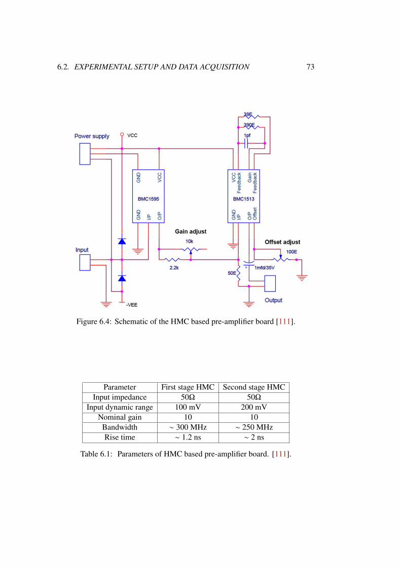
6.2. EXPERIMENTAL SETUP AND DATA ACQUISITION 73
Figure 6.4: Schematic of the HMC based pre-amplifier board [111].
Parameter First stage HMC Second stage HMCInput impedance 50Ω 50Ω
Input dynamic range 100 mV 200 mVNominal gain 10 10Bandwidth ∼ 300 MHz ∼ 250 MHzRise time ∼ 1.2 ns ∼ 2 ns
Table 6.1: Parameters of HMC based pre-amplifier board. [111].
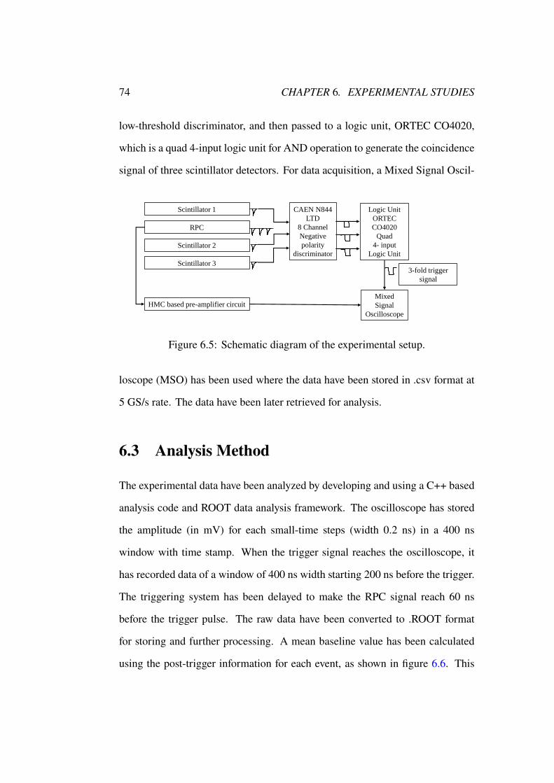
74 CHAPTER 6. EXPERIMENTAL STUDIES
low-threshold discriminator, and then passed to a logic unit, ORTEC CO4020,
which is a quad 4-input logic unit for AND operation to generate the coincidence
signal of three scintillator detectors. For data acquisition, a Mixed Signal Oscil-
Scintillator 1
RPC
Scintillator 3
Scintillator 2
CAEN N844
LTD
8 Channel
Negative
polarity
discriminator
Logic Unit
ORTEC
CO4020
Quad
4- input
Logic Unit
Mixed
Signal
Oscilloscope
3-fold trigger
signal
HMC based pre-amplifier circuit
Figure 6.5: Schematic diagram of the experimental setup.
loscope (MSO) has been used where the data have been stored in .csv format at
5 GS/s rate. The data have been later retrieved for analysis.
6.3 Analysis Method
The experimental data have been analyzed by developing and using a C++ based
analysis code and ROOT data analysis framework. The oscilloscope has stored
the amplitude (in mV) for each small-time steps (width 0.2 ns) in a 400 ns
window with time stamp. When the trigger signal reaches the oscilloscope, it
has recorded data of a window of 400 ns width starting 200 ns before the trigger.
The triggering system has been delayed to make the RPC signal reach 60 ns
before the trigger pulse. The raw data have been converted to .ROOT format
for storing and further processing. A mean baseline value has been calculated
using the post-trigger information for each event, as shown in figure 6.6. This
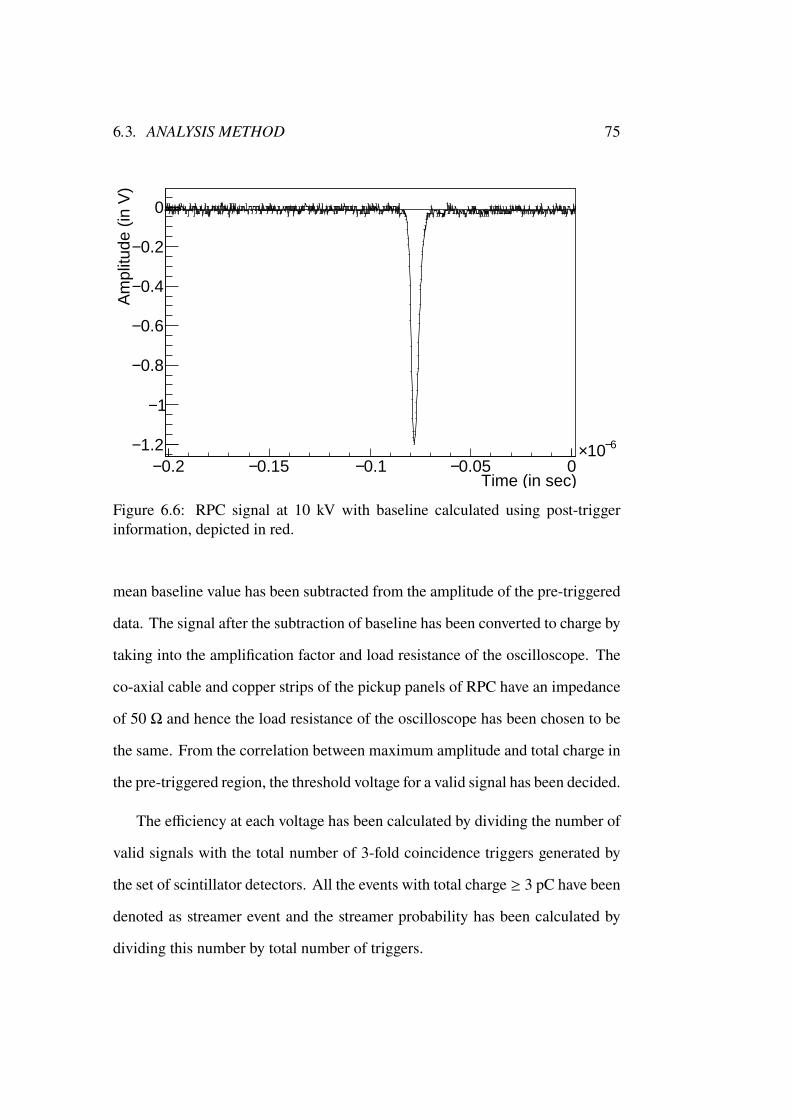
6.3. ANALYSIS METHOD 75
0.2− 0.15− 0.1− 0.05− 06−10×
Time (in sec)
1.2−
1−
0.8−
0.6−
0.4−
0.2−
0
Am
plitu
de (
in V
)
Figure 6.6: RPC signal at 10 kV with baseline calculated using post-triggerinformation, depicted in red.
mean baseline value has been subtracted from the amplitude of the pre-triggered
data. The signal after the subtraction of baseline has been converted to charge by
taking into the amplification factor and load resistance of the oscilloscope. The
co-axial cable and copper strips of the pickup panels of RPC have an impedance
of 50 Ω and hence the load resistance of the oscilloscope has been chosen to be
the same. From the correlation between maximum amplitude and total charge in
the pre-triggered region, the threshold voltage for a valid signal has been decided.
The efficiency at each voltage has been calculated by dividing the number of
valid signals with the total number of 3-fold coincidence triggers generated by
the set of scintillator detectors. All the events with total charge ≥ 3 pC have been
denoted as streamer event and the streamer probability has been calculated by
dividing this number by total number of triggers.
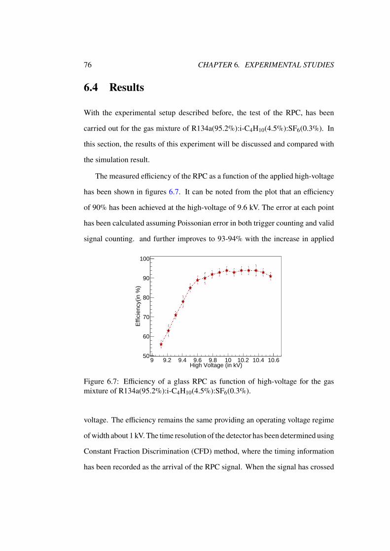
76 CHAPTER 6. EXPERIMENTAL STUDIES
6.4 Results
With the experimental setup described before, the test of the RPC, has been
carried out for the gas mixture of R134a(95.2%):i-C4H10(4.5%):SF6(0.3%). In
this section, the results of this experiment will be discussed and compared with
the simulation result.
The measured efficiency of the RPC as a function of the applied high-voltage
has been shown in figures 6.7. It can be noted from the plot that an efficiency
of 90% has been achieved at the high-voltage of 9.6 kV. The error at each point
has been calculated assuming Poissonian error in both trigger counting and valid
signal counting. and further improves to 93-94% with the increase in applied
9 9.2 9.4 9.6 9.8 10 10.2 10.4 10.6High Voltage (in kV)
50
60
70
80
90
100
Effi
cien
cy(in
%)
Figure 6.7: Efficiency of a glass RPC as function of high-voltage for the gasmixture of R134a(95.2%):i-C4H10(4.5%):SF6(0.3%).
voltage. The efficiency remains the same providing an operating voltage regime
ofwidth about 1 kV. The time resolution of the detector has been determined using
Constant Fraction Discrimination (CFD) method, where the timing information
has been recorded as the arrival of the RPC signal. When the signal has crossed
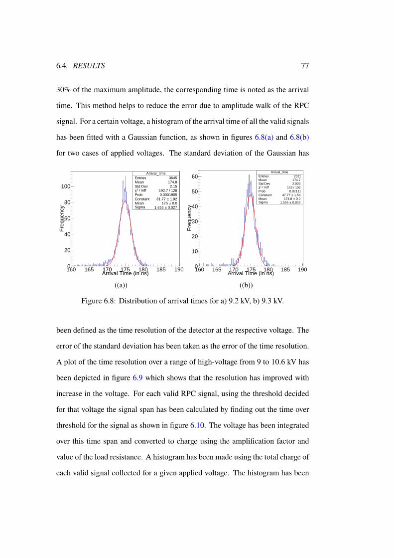
6.4. RESULTS 77
30% of the maximum amplitude, the corresponding time is noted as the arrival
time. This method helps to reduce the error due to amplitude walk of the RPC
signal. For a certain voltage, a histogram of the arrival time of all the valid signals
has been fitted with a Gaussian function, as shown in figures 6.8(a) and 6.8(b)
for two cases of applied voltages. The standard deviation of the Gaussian has
Arrival_timeEntries 3645Mean 174.8Std Dev 2.15
/ ndf 2χ 192.7 / 128Prob 0.0001905Constant 1.92± 81.77 Mean 0.0± 175 Sigma 0.027± 1.655
160 165 170 175 180 185 190Arrival Time (in ns)
0
20
40
60
80
100
Fre
quen
cy
Arrival_timeEntries 3645Mean 174.8Std Dev 2.15
/ ndf 2χ 192.7 / 128Prob 0.0001905Constant 1.92± 81.77 Mean 0.0± 175 Sigma 0.027± 1.655
((a))
Arrival_timeEntries 2021Mean 174.7Std Dev 2.003
/ ndf 2χ 133 / 102Prob 0.02111Constant 1.54± 47.77 Mean 0.0± 174.8 Sigma 0.035± 1.556
160 165 170 175 180 185 190Arrival Time (in ns)
0
10
20
30
40
50
60
Fre
quen
cy
Arrival_timeEntries 2021Mean 174.7Std Dev 2.003
/ ndf 2χ 133 / 102Prob 0.02111Constant 1.54± 47.77 Mean 0.0± 174.8 Sigma 0.035± 1.556
((b))
Figure 6.8: Distribution of arrival times for a) 9.2 kV, b) 9.3 kV.
been defined as the time resolution of the detector at the respective voltage. The
error of the standard deviation has been taken as the error of the time resolution.
A plot of the time resolution over a range of high-voltage from 9 to 10.6 kV has
been depicted in figure 6.9 which shows that the resolution has improved with
increase in the voltage. For each valid RPC signal, using the threshold decided
for that voltage the signal span has been calculated by finding out the time over
threshold for the signal as shown in figure 6.10. The voltage has been integrated
over this time span and converted to charge using the amplification factor and
value of the load resistance. A histogram has been made using the total charge of
each valid signal collected for a given applied voltage. The histogram has been
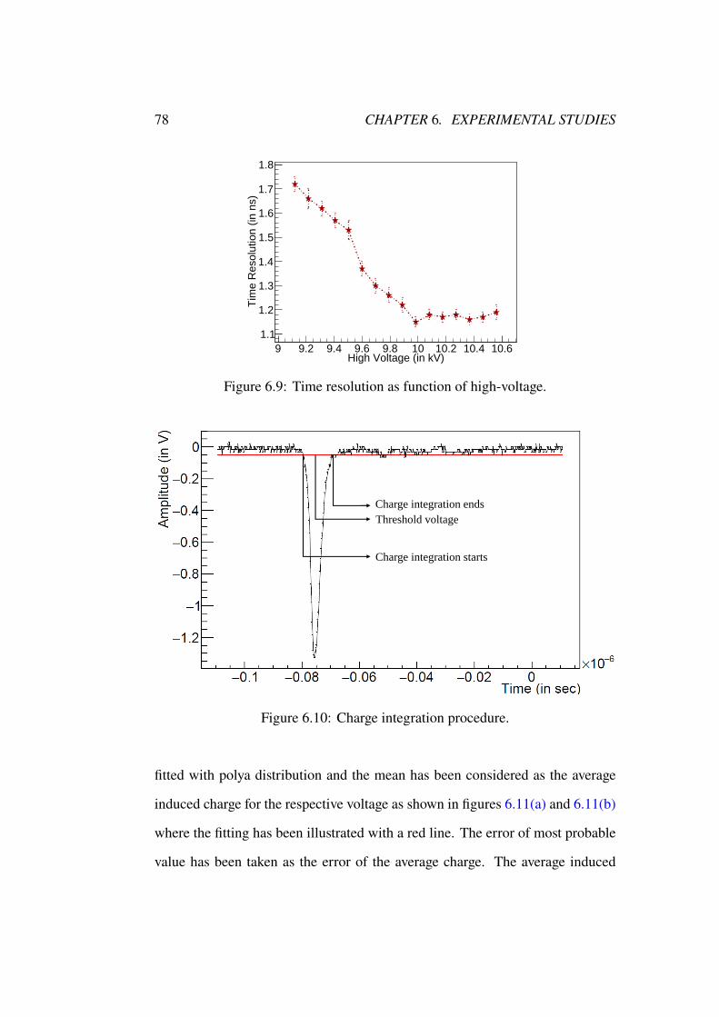
78 CHAPTER 6. EXPERIMENTAL STUDIES
9 9.2 9.4 9.6 9.8 10 10.2 10.4 10.6High Voltage (in kV)
1.1
1.2
1.3
1.4
1.5
1.6
1.7
1.8
Tim
e R
esol
utio
n (in
ns)
Figure 6.9: Time resolution as function of high-voltage.
Charge integration ends
Threshold voltage
Charge integration starts
Figure 6.10: Charge integration procedure.
fitted with polya distribution and the mean has been considered as the average
induced charge for the respective voltage as shown in figures 6.11(a) and 6.11(b)
where the fitting has been illustrated with a red line. The error of most probable
value has been taken as the error of the average charge. The average induced
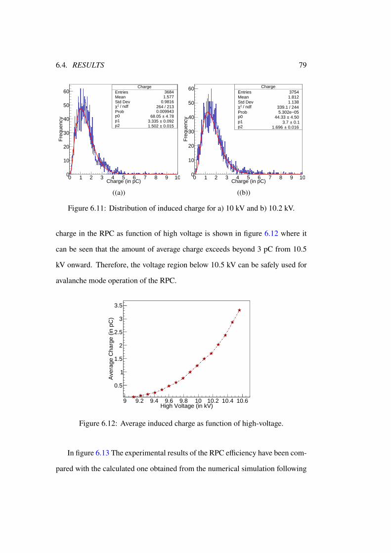
6.4. RESULTS 79
ChargeEntries 3684Mean 1.577Std Dev 0.9816
/ ndf 2χ 264 / 213Prob 0.009943p0 4.78± 68.05 p1 0.092± 3.335 p2 0.015± 1.502
0 1 2 3 4 5 6 7 8 9 10Charge (in pC)
0
10
20
30
40
50
60
Fre
quen
cy
ChargeEntries 3684Mean 1.577Std Dev 0.9816
/ ndf 2χ 264 / 213Prob 0.009943p0 4.78± 68.05 p1 0.092± 3.335 p2 0.015± 1.502
((a))
ChargeEntries 3754Mean 1.812Std Dev 1.138
/ ndf 2χ 339.1 / 244Prob 05− 5.302ep0 4.50± 44.33 p1 0.1± 3.7 p2 0.016± 1.696
0 1 2 3 4 5 6 7 8 9 10Charge (in pC)
0
10
20
30
40
50
60
Fre
quen
cy
ChargeEntries 3754Mean 1.812Std Dev 1.138
/ ndf 2χ 339.1 / 244Prob 05− 5.302ep0 4.50± 44.33 p1 0.1± 3.7 p2 0.016± 1.696
((b))
Figure 6.11: Distribution of induced charge for a) 10 kV and b) 10.2 kV.
charge in the RPC as function of high voltage is shown in figure 6.12 where it
can be seen that the amount of average charge exceeds beyond 3 pC from 10.5
kV onward. Therefore, the voltage region below 10.5 kV can be safely used for
avalanche mode operation of the RPC.
9 9.2 9.4 9.6 9.8 10 10.2 10.4 10.6High Voltage (in kV)
0.5
1
1.5
2
2.5
3
3.5
Ave
rage
Cha
rge
(in p
C)
Figure 6.12: Average induced charge as function of high-voltage.
In figure 6.13 The experimental results of the RPC efficiency have been com-
pared with the calculated one obtained from the numerical simulation following
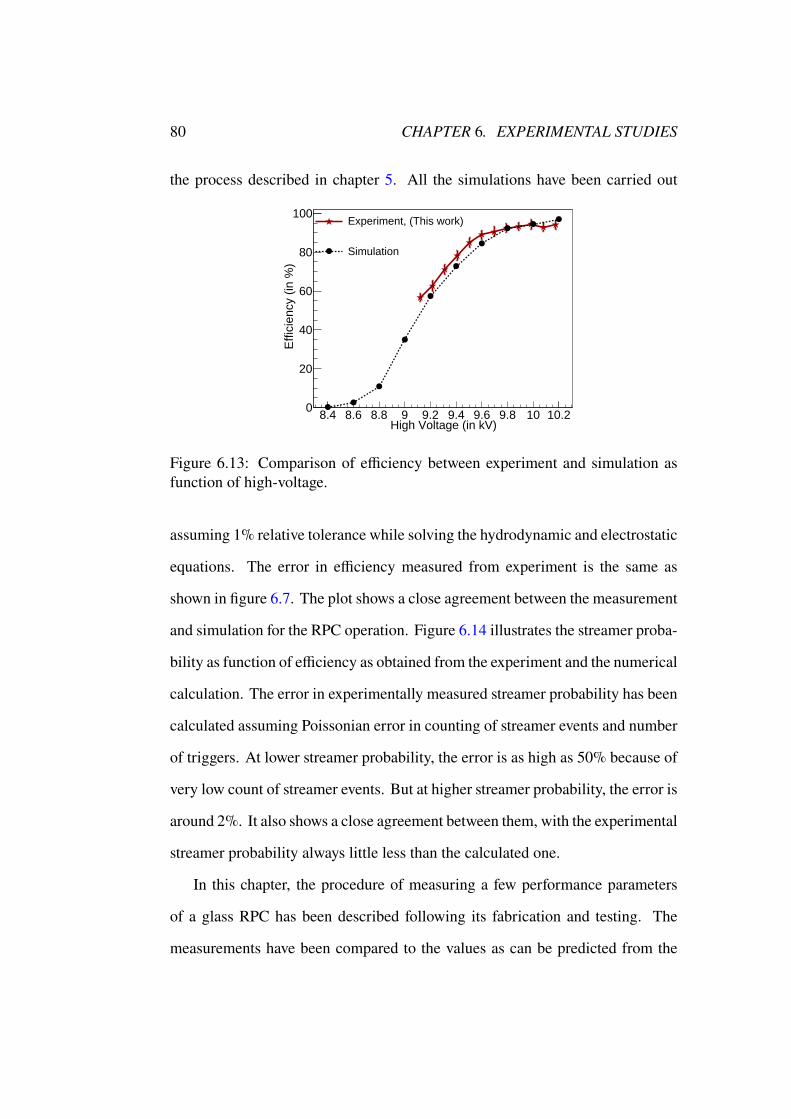
80 CHAPTER 6. EXPERIMENTAL STUDIES
the process described in chapter 5. All the simulations have been carried out
8.4 8.6 8.8 9 9.2 9.4 9.6 9.8 10 10.2High Voltage (in kV)
0
20
40
60
80
100
Effi
cien
cy (
in %
)
Experiment, (This work)
Simulation
Figure 6.13: Comparison of efficiency between experiment and simulation asfunction of high-voltage.
assuming 1% relative tolerance while solving the hydrodynamic and electrostatic
equations. The error in efficiency measured from experiment is the same as
shown in figure 6.7. The plot shows a close agreement between the measurement
and simulation for the RPC operation. Figure 6.14 illustrates the streamer proba-
bility as function of efficiency as obtained from the experiment and the numerical
calculation. The error in experimentally measured streamer probability has been
calculated assuming Poissonian error in counting of streamer events and number
of triggers. At lower streamer probability, the error is as high as 50% because of
very low count of streamer events. But at higher streamer probability, the error is
around 2%. It also shows a close agreement between them, with the experimental
streamer probability always little less than the calculated one.
In this chapter, the procedure of measuring a few performance parameters
of a glass RPC has been described following its fabrication and testing. The
measurements have been compared to the values as can be predicted from the

6.4. RESULTS 81
0 20 40 60 80 100Efficiency (in %)
0
2
4
6
8
10
12
Str
eam
er P
roba
bilit
y (in
%)
Experiment, (This work)
Simulation
Figure 6.14: Comparison of streamer probability between experiment and simu-lation as function of high-voltage.
numerical simulation of the RPC dynamics following hydrodynamic approach.
A close agreement between the experiment and simulation has implied that the
hydrodynamic model devised for the RPC is reasonably successful in emulating
its working procedure. The finding has prompted utilization of the numerical
model in exploring new gas mixtures and their feasibility for operating the RPCs
of the ICAL in avalanche mode in order to address the environmental issues of
the present

82 CHAPTER 6. EXPERIMENTAL STUDIES
Chapter 7Numerical Qualification of
Eco-Friendly Gas Mixture
The need for eco-friendly RPC operation in INO-ICAL has motivated the investi-
gation for an alternate feasible gas mixture. In this context, the numerical model,
described in the chapter 5, has been used to numerically qualify such a mixture.
It has been shown in chapters 5 and 6 that the model can emulate the working
mode of the RPC at different applied voltages for a given filling gas mixture,
from which its efficiency and the streamer probability can be estimated. In this
chapter the ability of the numerical model in simulating the charge evolution
reliably has been utilized to test an alternative gas mixture which needs to be
eco-friendly, non-flammable, economical for operating 28,800 RPCs of ICAL
in avalanche mode over a long period of time. It is important to predict their
efficiency and the streamer probability as figures of merit to plan and design the
experimental accessories. In the following, a brief discussion on the gas studies
will be provided first to justify the choice of gas components to propose a new
83
84CHAPTER 7. NUMERICAL QUALIFICATION OF ECO-FRIENDLY GAS
MIXTURE
mixture. Later the simulated performance of the RPC for the proposed mixture
will be presented and compared to the simulated values of the same observable
for a standard mixture of R134a (95.2%):i-C4H10 (4.5%):SF6 (0.3%) to demon-
strate the merits and demerits of the new mixture. It should be noted that the
simulated RPC responses for the standard R134a-based mixture have shown a
close agreement with the experimental measurements as discussed in chapter
6. The same will be done for other potential eco-friendly Hydro-Fluoro-Olefin
(HFO)-based gas mixtures too.
7.1 Choice of Gas Mixture
Extensive studies on various gases and their properties in order to find suitable
substitutes for operating RPCs in many other high energy physics experiments
[106, 107, 112, 113, 114, 115, 116] have been carried out. According to these
studies, one allotropic form of tetrafluoropropene, C3H2F4 (commercially known
as HFO1234ze) which is close to R134a in chemical structure, with very low
GWP (∼ 6), can be regarded as a potential replacement. However, theHFO1234ze
shows lower effective Townsend coefficient with respect to that of R134a when
compared at the same electric field. As a consequence, comparatively higher
electric field is required to achieve an efficiency of about 90%. A few promising
mixtures based on HFO1234ze, i-C4H10 and He or CO2 could be identified with
low GWP (< 150) [112, 116] for efficient operation of RPC, though the high
voltage requirement of some of them [116] might not be compatible to ICAL
high voltage supply system [117]. Moreover, thesemixtures have shown presence
of substantially large fraction of streamers [112, 116] at higher efficiency, which
7.1. CHOICE OF GAS MIXTURE 85
is well above the tolerable limit for safe and long term operation. As a result,
inclusion of small amount of electron quencher gas SF6 (∼ 1%) in the mixtures
could not be ruled out for efficient operation of the detectors, which has led the
effective GWP sometimes cross the limit of 150 [106, 107, 112, 115]. Other
than this, HFO1234ze has one more disadvantage regarding its use in RPC,
considering the criticism about its degrading effect on the detector health. It
has low GWP, essentially because of its smaller lifetime in the environment.
The rate of dissociation of the gas in presence of OH− radical (produced from
dissociation of water molecule) is four times faster than that of R134a [118]. The
final products are HF and other corrosive acids, which can destroy the surface
of the RPC electrodes. For neutrino experiments which will operate for long
time, consistent detector performance and in turn good health of the detector is
an important requirement.
In this doctoral study, a gas mixture of Ar, CO2 and N2 in volume percentage
of 5:60:35 has been proposed as a new alternative for avalanche mode operation
of RPCs. It should be noted that all the components other than CO2 (GWP = 1)
are green (GWP = 0) and commercially available economical gases. The argon
has been taken as the principal component for ionization. Its high Townsend
coefficient at low electric field will help to reduce the operating voltage of RPCs.
On the other hand, it will lead to large streamer probability at higher fields. To
circumvent the issue of streamer, the partial volume of the Ar has been reduced
by introducing N2 which is highly electronegative and chemically less reactive.
As a photon quencher, CO2 has been preferred over other alternatives as it has
less penning transfer coefficient in a mixture with Ar [119] and less GWP [114].
Its non-flammability and cheap cost are the added advantages.
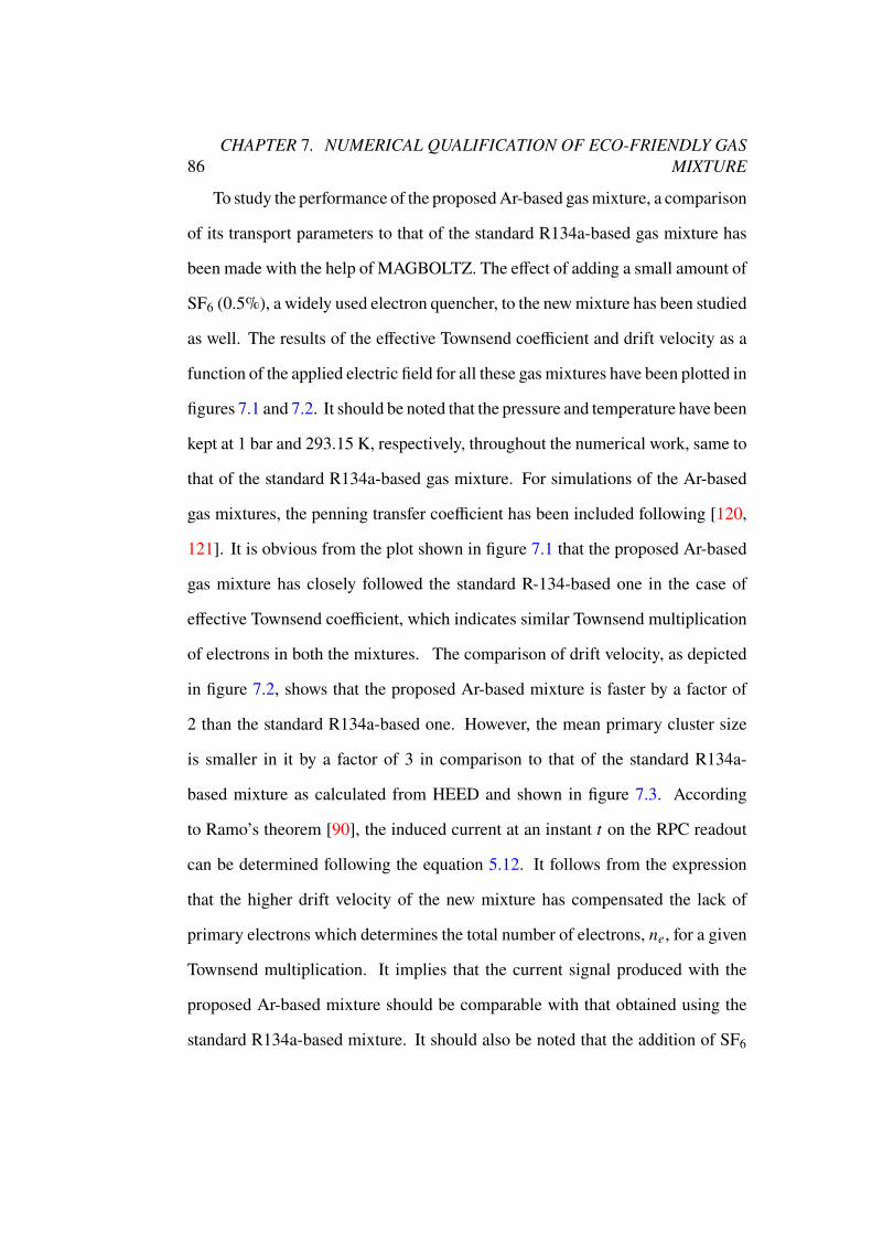
86CHAPTER 7. NUMERICAL QUALIFICATION OF ECO-FRIENDLY GAS
MIXTURE
To study the performance of the proposedAr-based gasmixture, a comparison
of its transport parameters to that of the standard R134a-based gas mixture has
been made with the help of MAGBOLTZ. The effect of adding a small amount of
SF6 (0.5%), a widely used electron quencher, to the newmixture has been studied
as well. The results of the effective Townsend coefficient and drift velocity as a
function of the applied electric field for all these gas mixtures have been plotted in
figures 7.1 and 7.2. It should be noted that the pressure and temperature have been
kept at 1 bar and 293.15 K, respectively, throughout the numerical work, same to
that of the standard R134a-based gas mixture. For simulations of the Ar-based
gas mixtures, the penning transfer coefficient has been included following [120,
121]. It is obvious from the plot shown in figure 7.1 that the proposed Ar-based
gas mixture has closely followed the standard R-134-based one in the case of
effective Townsend coefficient, which indicates similar Townsend multiplication
of electrons in both the mixtures. The comparison of drift velocity, as depicted
in figure 7.2, shows that the proposed Ar-based mixture is faster by a factor of
2 than the standard R134a-based one. However, the mean primary cluster size
is smaller in it by a factor of 3 in comparison to that of the standard R134a-
based mixture as calculated from HEED and shown in figure 7.3. According
to Ramo’s theorem [90], the induced current at an instant C on the RPC readout
can be determined following the equation 5.12. It follows from the expression
that the higher drift velocity of the new mixture has compensated the lack of
primary electrons which determines the total number of electrons, =4, for a given
Townsend multiplication. It implies that the current signal produced with the
proposed Ar-based mixture should be comparable with that obtained using the
standard R134a-based mixture. It should also be noted that the addition of SF6
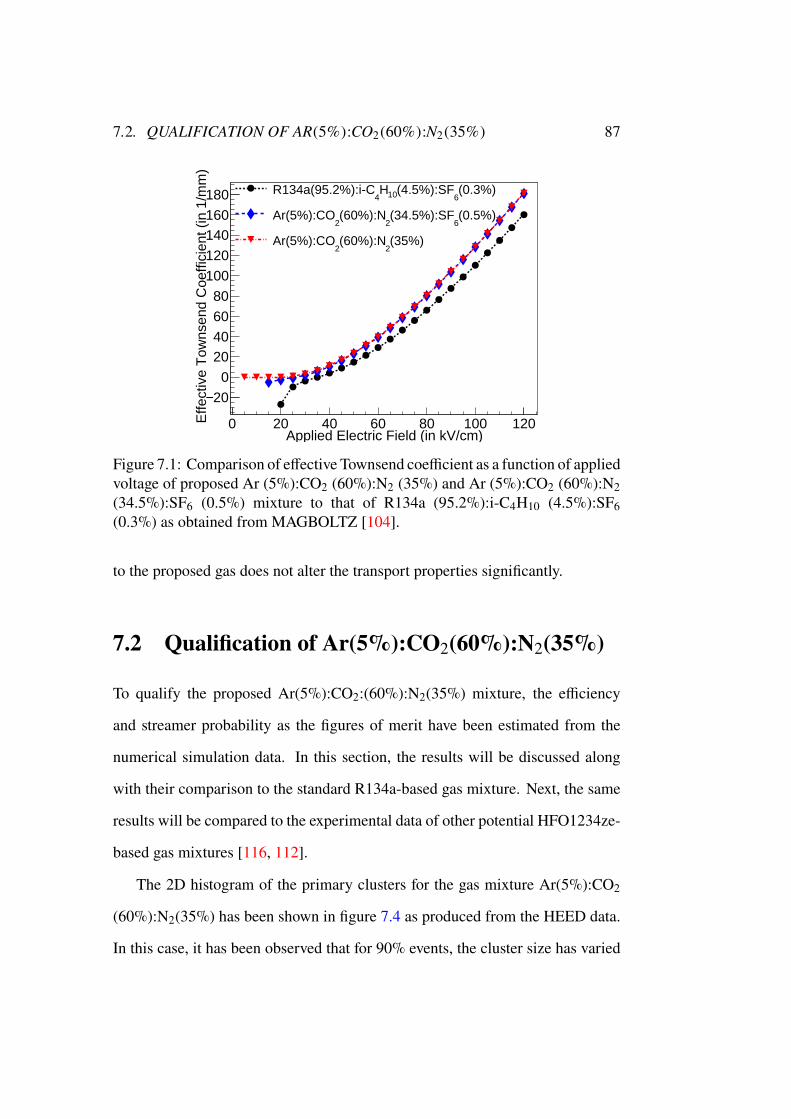
7.2. QUALIFICATION OF AR(5%):CO2(60%):N2(35%) 87
0 20 40 60 80 100 120Applied Electric Field (in kV/cm)
20−0
2040
60
80
100
120
140160
180 E
ffect
ive
Tow
nsen
d C
oeffi
cien
t (in
1/m
m)
(0.3%)6
(4.5%):SF10H4
R134a(95.2%):i-C
(0.5%)6
(34.5%):SF2
(60%):N2
Ar(5%):CO
(35%)2
(60%):N2
Ar(5%):CO
Figure 7.1: Comparison of effective Townsend coefficient as a function of appliedvoltage of proposed Ar (5%):CO2 (60%):N2 (35%) and Ar (5%):CO2 (60%):N2(34.5%):SF6 (0.5%) mixture to that of R134a (95.2%):i-C4H10 (4.5%):SF6(0.3%) as obtained from MAGBOLTZ [104].
to the proposed gas does not alter the transport properties significantly.
7.2 Qualification of Ar(5%):CO2(60%):N2(35%)
To qualify the proposed Ar(5%):CO2:(60%):N2(35%) mixture, the efficiency
and streamer probability as the figures of merit have been estimated from the
numerical simulation data. In this section, the results will be discussed along
with their comparison to the standard R134a-based gas mixture. Next, the same
results will be compared to the experimental data of other potential HFO1234ze-
based gas mixtures [116, 112].
The 2D histogram of the primary clusters for the gas mixture Ar(5%):CO2
(60%):N2(35%) has been shown in figure 7.4 as produced from the HEED data.
In this case, it has been observed that for 90% events, the cluster size has varied
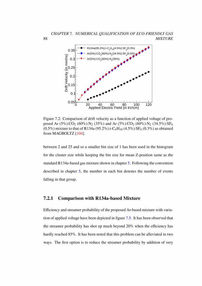
88CHAPTER 7. NUMERICAL QUALIFICATION OF ECO-FRIENDLY GAS
MIXTURE
0 20 40 60 80 100 120Applied Electric Field (in kV/cm)
0.05
0.1
0.15
0.2
0.25
0.3
0.35
Drif
t Vel
ocity
(in
mm
/ns)
(0.3%)6
(4.5%):SF10H4
R134a(95.2%):i-C
(0.5%)6
(34.5%):SF2
(60%):N2
Ar(5%):CO
(35%)2
(60%):N2
Ar(5%):CO
Figure 7.2: Comparison of drift velocity as a function of applied voltage of pro-posed Ar (5%):CO2 (60%):N2 (35%) and Ar (5%):CO2 (60%):N2 (34.5%):SF6(0.5%) mixture to that of R134a (95.2%):i-C4H10 (4.5%):SF6 (0.3%) as obtainedfrom MAGBOLTZ [104].
between 2 and 25 and so a smaller bin size of 1 has been used in the histogram
for the cluster size while keeping the bin size for mean Z-position same as the
standard R134a-based gas mixture shown in chapter 5. Following the convention
described in chapter 5, the number in each bin denotes the number of events
falling in that group.
7.2.1 Comparison with R134a-based Mixture
Efficiency and streamer probability of the proposed Ar-based mixture with varia-
tion of applied voltage have been depicted in figure 7.5. It has been observed that
the streamer probability has shot up much beyond 20% when the efficiency has
hardly reached 85%. It has been noted that this problem can be alleviated in two
ways. The first option is to reduce the streamer probability by addition of very
7.2. QUALIFICATION OF AR(5%):CO2(60%):N2(35%) 89
10 20 30 40 50 60 70 80 90 100Number of Primary electrons
0
100
200
300
400
500
600
700
800F
requ
ency
(35%)2
(60%):N2
Ar(5%):CO
(0.5%)6
(34.5%):SF2
(60%):N2
Ar(5%):CO
(0.3%)6
(4.5%):SF10H4
R134a(95.2%):i-C
Figure 7.3: Comparison of primary electron number of proposed Ar (5%):CO2(60%):N2 (35%) and Ar (5%):CO2 (60%):N2 (34.5%):SF6 (0.5%)mixture to thatof R134a (95.2%):i-C4H10 (4.5%):SF6 (0.3%) as obtained from HEED [103].The values have been calculated assuming the gas temperature is 293.15K andpressure 1 bar.
small amount of electronegative SF6 as practiced in case of the standard R134a-
based mixture. Nevertheless, this option should not be very much effective, as
implied by the plot shown in figure 7.1. The GWP of the Ar-based mixture will
be within the limit of 150 if SF6 is added by a percentage of less than 0.5%.
The other option is to reduce the threshold for valid event to increase the ratio of
the avalanche events to the streamer one, which will obviously allow some noise
eventually. Both the options have been studied, and the expected improvement
has been observed in both the cases. The effect of adding 0.5% of SF6 in the
mixture has been depicted in figure 7.6(a) where the efficiency of the mixture
with and without the SF6 component has been compared to that of the standard
mixture. It can be noted from the figure that the operation in avalanchemodewith

90CHAPTER 7. NUMERICAL QUALIFICATION OF ECO-FRIENDLY GAS
MIXTURE
5 2 8 6 13 17 13 16 20 35 20 26 26 10 7 9 6 52 7 8 22 25 19 27 52 45 51 44 37 23 16 8 10 3 54 1 8 24 34 51 57 55 69 57 56 48 40 33 18 10 5 11 2 7 25 35 66 78 71 86 78 83 65 49 30 16 7 32 3 5 17 28 43 71 107 101109 100 90 42 29 19 7 2
3 8 34 45 78 105 130 126 98 79 45 29 11 7 11 1 5 17 25 46 82 90 117 99 93 89 55 27 15 9 4 1
1 2 10 22 34 61 109 94 110 95 88 53 28 4 61 6 6 24 37 69 88 103 93 67 85 39 28 10 6
1 5 11 25 33 52 70 95 79 76 41 34 19 8 2 21 4 10 10 24 45 57 77 71 62 40 34 18 7 6 1 11 6 2 14 24 36 49 60 55 43 39 19 15 7 11 2 7 15 16 26 52 49 44 36 43 15 8 2 4
2 1 4 6 15 22 32 40 31 22 25 15 10 10 62 3 8 14 21 21 34 34 23 18 12 6 2 3 1
1 7 4 9 8 10 19 19 18 30 11 13 8 4 1 11 3 6 3 14 16 15 17 23 20 12 9 13 5 2 11 2 2 3 8 8 7 19 16 19 12 8 7 11 7 3
3 6 7 9 13 10 10 13 17 8 6 3 3 3 2 11 1 1 4 10 11 5 10 11 11 14 8 12 2 2 2 31 3 1 5 3 4 8 10 9 15 6 5 13 6 3 2 2
1 4 3 6 4 9 5 11 12 8 12 7 7 3 32 3 4 4 14 3 8 6 5 7 11 6 6 4 21 4 5 2 12 8 3 10 8 5 9 10 6 1 1 2
0.2 0.4 0.6 0.8 1 1.2 1.4 1.6 1.8Mean Z-position (in mm)
5
10
15
20
25
Tot
al N
umbe
r of
Ele
ctro
ns
(35%)2
(60%):N2
Ar(5%):CO
Figure 7.4: 2D histogram of muon events for the gas mixture of Ar(5%):CO2(60%):N2(35%).
the Ar-based mixture is not practically feasible beyond 80-85% efficiency. The
addition of SF6 component in the mixture has reduced the streamer probability
by 40% at this efficiency range, although it is still higher in comparison to the
standard R134a-based mixture. The results of reducing the threshold from 5 mV
to 1 mV have been depicted in figure 7.6(b) where an overall reduction in the
streamer probability of the Ar-based mixture is visible. This approach can lead
to an acceptable streamer probability (< 10%) around 85% efficiency, which is
comparable to that of the standard R134a-based mixture. It can be noted that by
reducing the threshold, the present Ar-based mixture can operate efficiently with
low streamer probability even without the SF6 component.
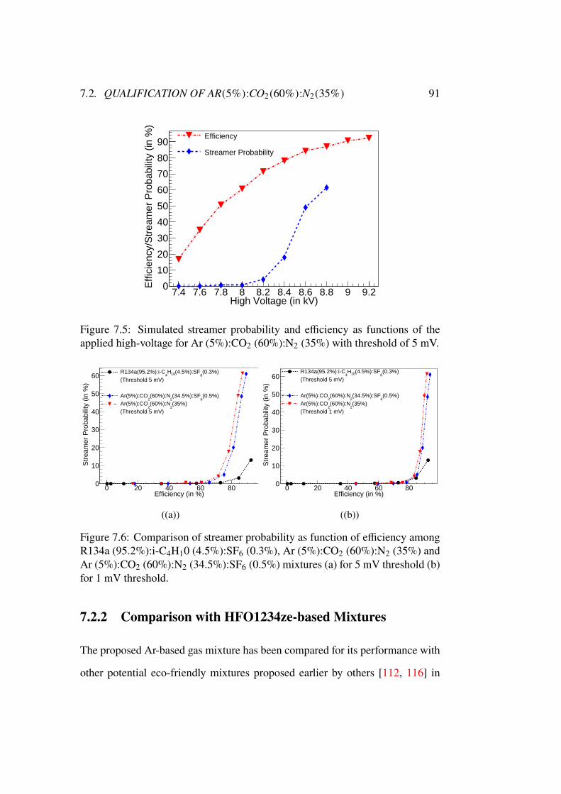
7.2. QUALIFICATION OF AR(5%):CO2(60%):N2(35%) 91
7.4 7.6 7.8 8 8.2 8.4 8.6 8.8 9 9.2High Voltage (in kV)
0
10
20
30
40
50
60
70
80
90 E
ffici
ency
/Str
eam
er P
roba
bilit
y (in
%)
Efficiency
Streamer Probability
Figure 7.5: Simulated streamer probability and efficiency as functions of theapplied high-voltage for Ar (5%):CO2 (60%):N2 (35%) with threshold of 5 mV.
0 20 40 60 80Efficiency (in %)
0
10
20
30
40
50
60
Str
eam
er P
roba
bilit
y (in
%)
(0.3%)6
(4.5%):SF10H4
R134a(95.2%):i-C(Threshold 5 mV)
(0.5%)6
(34.5%):SF2
(60%):N2
Ar(5%):CO(35%)
2(60%):N
2Ar(5%):CO(Threshold 5 mV)
((a))
0 20 40 60 80Efficiency (in %)
0
10
20
30
40
50
60
Str
eam
er P
roba
bilit
y (in
%)
(0.3%)6
(4.5%):SF10H4
R134a(95.2%):i-C(Threshold 5 mV)
(0.5%)6
(34.5%):SF2
(60%):N2
Ar(5%):CO(35%)
2(60%):N
2Ar(5%):CO(Threshold 1 mV)
((b))
Figure 7.6: Comparison of streamer probability as function of efficiency amongR134a (95.2%):i-C4H10 (4.5%):SF6 (0.3%), Ar (5%):CO2 (60%):N2 (35%) andAr (5%):CO2 (60%):N2 (34.5%):SF6 (0.5%) mixtures (a) for 5 mV threshold (b)for 1 mV threshold.
7.2.2 Comparison with HFO1234ze-based Mixtures
The proposed Ar-based gas mixture has been compared for its performance with
other potential eco-friendly mixtures proposed earlier by others [112, 116] in
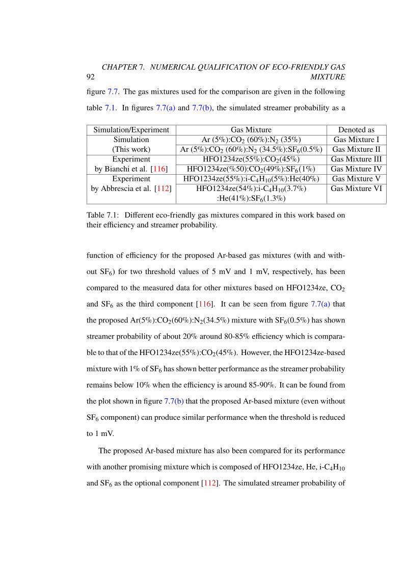
92CHAPTER 7. NUMERICAL QUALIFICATION OF ECO-FRIENDLY GAS
MIXTURE
figure 7.7. The gas mixtures used for the comparison are given in the following
table 7.1. In figures 7.7(a) and 7.7(b), the simulated streamer probability as a
Simulation/Experiment Gas Mixture Denoted asSimulation Ar (5%):CO2 (60%):N2 (35%) Gas Mixture I(This work) Ar (5%):CO2 (60%):N2 (34.5%):SF6(0.5%) Gas Mixture IIExperiment HFO1234ze(55%):CO2(45%) Gas Mixture III
by Bianchi et al. [116] HFO1234ze(%50):CO2(49%):SF6(1%) Gas Mixture IVExperiment HFO1234ze(55%):i-C4H10(5%):He(40%) Gas Mixture V
by Abbrescia et al. [112] HFO1234ze(54%):i-C4H10(3.7%) Gas Mixture VI:He(41%):SF6(1.3%)
Table 7.1: Different eco-friendly gas mixtures compared in this work based ontheir efficiency and streamer probability.
function of efficiency for the proposed Ar-based gas mixtures (with and with-
out SF6) for two threshold values of 5 mV and 1 mV, respectively, has been
compared to the measured data for other mixtures based on HFO1234ze, CO2
and SF6 as the third component [116]. It can be seen from figure 7.7(a) that
the proposed Ar(5%):CO2(60%):N2(34.5%) mixture with SF6(0.5%) has shown
streamer probability of about 20% around 80-85% efficiency which is compara-
ble to that of the HFO1234ze(55%):CO2(45%). However, the HFO1234ze-based
mixture with 1% of SF6 has shown better performance as the streamer probability
remains below 10% when the efficiency is around 85-90%. It can be found from
the plot shown in figure 7.7(b) that the proposed Ar-based mixture (even without
SF6 component) can produce similar performance when the threshold is reduced
to 1 mV.
The proposed Ar-based mixture has also been compared for its performance
with another promising mixture which is composed of HFO1234ze, He, i-C4H10
and SF6 as the optional component [112]. The simulated streamer probability of
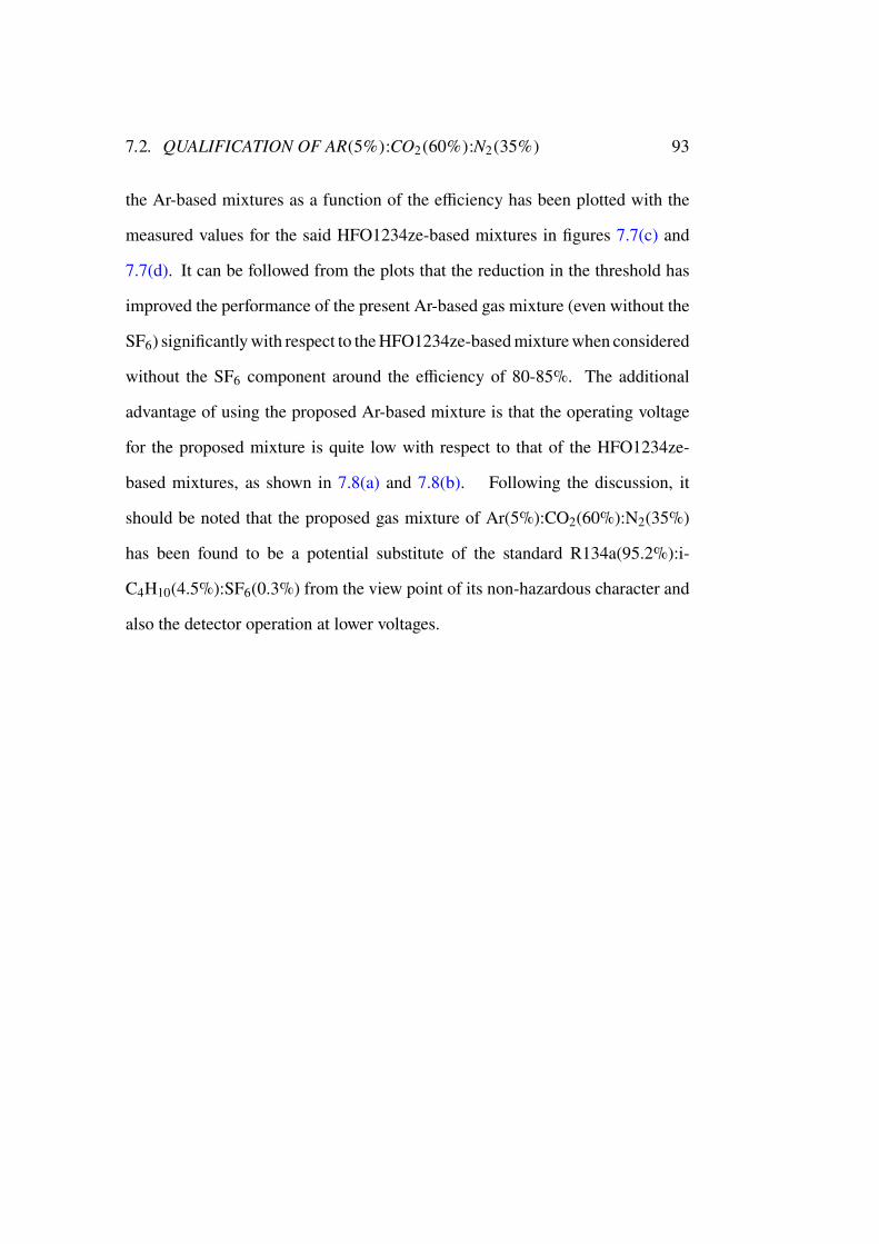
7.2. QUALIFICATION OF AR(5%):CO2(60%):N2(35%) 93
the Ar-based mixtures as a function of the efficiency has been plotted with the
measured values for the said HFO1234ze-based mixtures in figures 7.7(c) and
7.7(d). It can be followed from the plots that the reduction in the threshold has
improved the performance of the present Ar-based gas mixture (even without the
SF6) significantlywith respect to theHFO1234ze-basedmixturewhen considered
without the SF6 component around the efficiency of 80-85%. The additional
advantage of using the proposed Ar-based mixture is that the operating voltage
for the proposed mixture is quite low with respect to that of the HFO1234ze-
based mixtures, as shown in 7.8(a) and 7.8(b). Following the discussion, it
should be noted that the proposed gas mixture of Ar(5%):CO2(60%):N2(35%)
has been found to be a potential substitute of the standard R134a(95.2%):i-
C4H10(4.5%):SF6(0.3%) from the view point of its non-hazardous character and
also the detector operation at lower voltages.
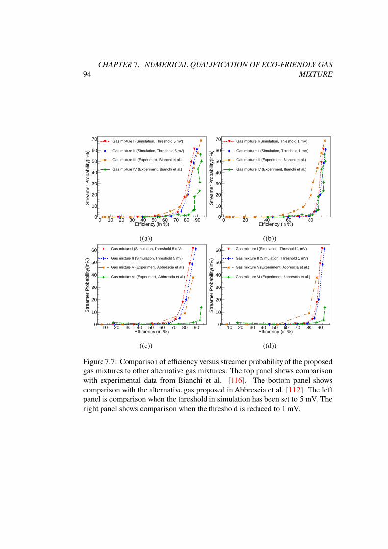
94CHAPTER 7. NUMERICAL QUALIFICATION OF ECO-FRIENDLY GAS
MIXTURE
0 10 20 30 40 50 60 70 80 90Efficiency (in %)
0
10
20
30
40
50
60
70
Str
eam
er P
roba
bilit
y(in
%)
Gas mixture I (Simulation, Threshold 5 mV)
Gas mixture II (Simulation, Threshold 5 mV)
Gas mixture III (Experiment, Bianchi et al.)
Gas mixture IV (Experiment, Bianchi et al.)
((a))
0 20 40 60 80Efficiency (in %)
0
10
20
30
40
50
60
70
Str
eam
er P
roba
bilit
y(in
%)
Gas mixture I (Simulation, Threshold 1 mV)
Gas mixture II (Simulation, Threshold 1 mV)
Gas mixture III (Experiment, Bianchi et al.)
Gas mixture IV (Experiment, Bianchi et al.)
((b))
10 20 30 40 50 60 70 80 90Efficiency (in %)
0
10
20
30
40
50
60
Str
eam
er P
roba
bilit
y(in
%)
Gas mixture I (Simulation, Threshold 5 mV)
Gas mixture II (Simulation, Threshold 5 mV)
Gas mixture V (Experiment, Abbrescia et al.)
Gas mixture VI (Experiment, Abbrescia et al.)
((c))
10 20 30 40 50 60 70 80 90Efficiency (in %)
0
10
20
30
40
50
60
Str
eam
er P
roba
bilit
y(in
%)
Gas mixture I (Simulation, Threshold 1 mV)
Gas mixture II (Simulation, Threshold 1 mV)
Gas mixture V (Experiment, Abbrescia et al.)
Gas mixture VI (Experiment, Abbrescia et al.)
((d))
Figure 7.7: Comparison of efficiency versus streamer probability of the proposedgas mixtures to other alternative gas mixtures. The top panel shows comparisonwith experimental data from Bianchi et al. [116]. The bottom panel showscomparison with the alternative gas proposed in Abbrescia et al. [112]. The leftpanel is comparison when the threshold in simulation has been set to 5 mV. Theright panel shows comparison when the threshold is reduced to 1 mV.
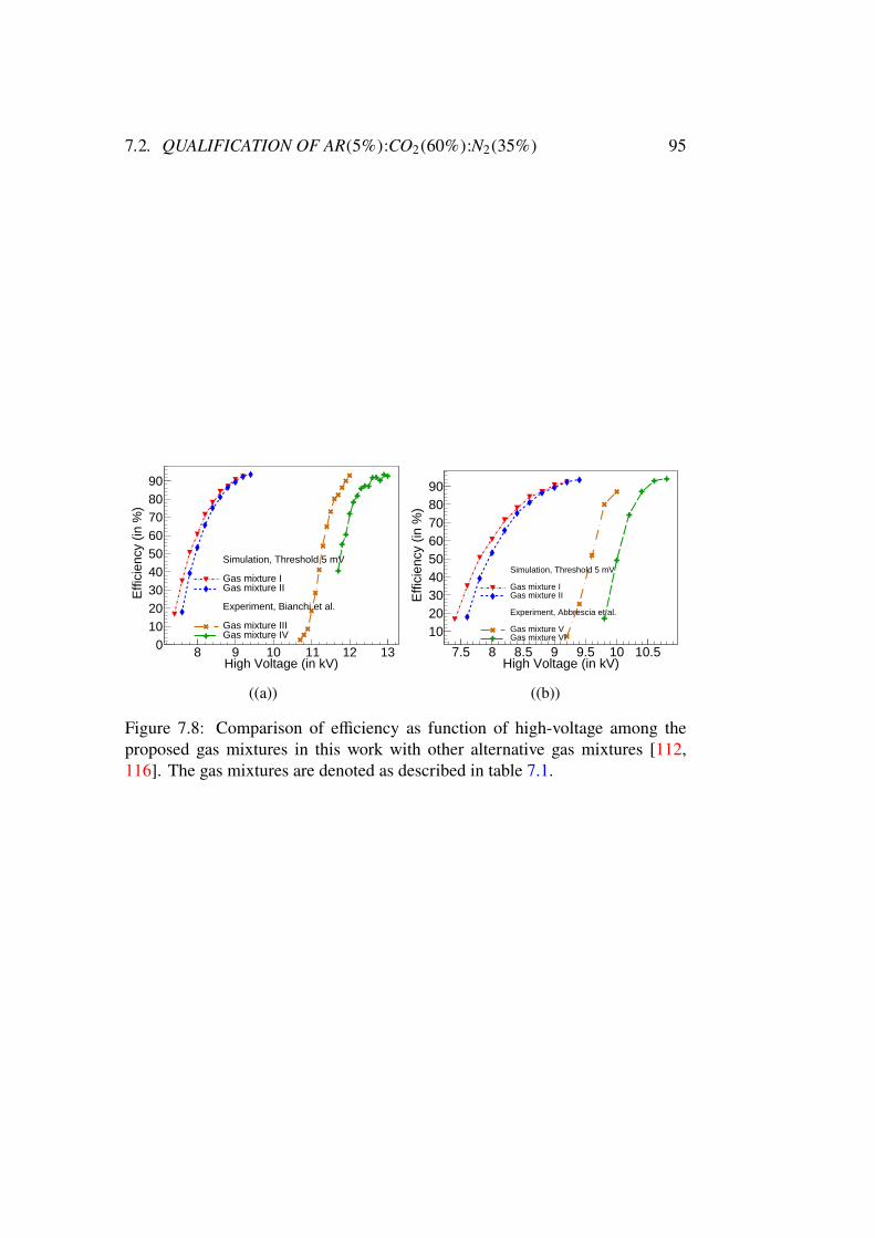
7.2. QUALIFICATION OF AR(5%):CO2(60%):N2(35%) 95
8 9 10 11 12 13High Voltage (in kV)
0102030405060708090
Effi
cien
cy (
in %
)
Simulation, Threshold 5 mV
Gas mixture IGas mixture II
Experiment, Bianchi et al.
Gas mixture IIIGas mixture IV
((a))
7.5 8 8.5 9 9.5 10 10.5High Voltage (in kV)
102030405060708090
Effi
cien
cy (
in %
)
Simulation, Threshold 5 mV
Gas mixture IGas mixture II
Experiment, Abbrescia et al.
Gas mixture VGas mixture VI
((b))
Figure 7.8: Comparison of efficiency as function of high-voltage among theproposed gas mixtures in this work with other alternative gas mixtures [112,116]. The gas mixtures are denoted as described in table 7.1.

Part II
Study of different aspects of
neutrino oscillation for ICAL at
INO
97


Chapter 8Neutrino Oscillations in Vacuum
and in Matter
The signature of non-zero mass of neutrino was established with the discovery of
the neutrino oscillation phenomena. The SM neutrinos have zero mass, so these
phenomena is a direct proof of the physics beyond SM. This chapter will describe
these phenomena and discuss the implications of different results. With the LEP
experiment, it was established that the number of light neutrino family is exactly
three. So it was evident that the all these three families interact through weak
interaction. Each of the families is called a flavor, and the states are called flavor
states. Following the ◦ ↔ ◦ oscillation, Pontecorvo first proposed the a ↔ a
oscillation. At that time, only the existence of a4 was established. Later, Maki-
Nakagawa-Sakata proposed an oscillation framework where the weak interaction
flavor states are linear superposition of the mass eigenstates. The basic idea of
this framework is that the neutrinos have mass and the flavor states do not overlap
with mass eigenstates. Following this idea, many contributed to formalize the
99
100CHAPTER 8. NEUTRINO OSCILLATIONS IN VACUUM AND IN MATTER
neutrino oscillation picture. At that time the ag was yet to be discovered, and
in the absence of ag initially the oscillation framework was built for two flavors,
a4, a`.
8.1 Neutrino oscillation in vacuum
8.1.1 Two Flavor Oscillation
In this formalism it is assumed that there are two mass eigenstates namely a1, a2
with mass <1 and <2 respectively. The flavor states are a4 and a`. The relation
between flavor andmass eigenstates can be expressed with the following equationa4
a`
=
cos \ sin \
− sin \ cos \
a1
a2
(8.1)
Now let’s assume in an interaction the created neutrino is a4. So at time t = 0,
the neutrino state |a〉 can be expressed as
|a(0)〉 = |a4〉 = cos \ |a1(0)〉 + sin \ |a2(0)〉 (8.2)
The time evolved neutrino state at t = t can be expressed using the following
equation,
|a(C)〉 = cos \ |a1(0)〉 4−8�1C + sin \ |a2(0)〉 4−8�2C (8.3)
where �1 and �2 are the energy of the mass eigenstates. So the projection of the
time evolved state on |a4〉 can be expressed as
〈a4 |a(C)〉 = cos \ 〈a4 |a1(0)〉 4−8�1C + sin \ 〈a4 |a2(0)〉 4−8�2C
= cos2 \4−8�1C + sin2 \4−8�2C (8.4)
8.1. NEUTRINO OSCILLATION IN VACUUM 101
and the same on a` can be expressed as
〈a` |a(C)〉 = cos \ 〈a` |a1(0)〉 4−8�1C + sin \ 〈a` |a2(0)〉 4−8�2C
= cos \ sin \ (4−8�2C − 4−8�1C) (8.5)
So the probability of observing a` after time t is
= | 〈a` |a(C)〉 |2
= sin2 2\ sin2((�2 − �1)C
2
)(8.6)
Now the energy of the mass eigenstates are �8 =√?28+ <2
8, ?8 and <8 is momen-
tum and mass of the 8Cℎ eigenstate. The neutrinos are ultra relativistic and their
mass is negligible. So the energy of the mass eigenstates can be approximated as
�8 = ?8 +<28
2?8 . The two mass eigenstate in principal can have different momenta,
but it can be shown that approximating the momentum of the two states to be
equal leaves the expression of the probability to be qualitatively the same. So
one can approximate that the momentum of the neutrino, ? = ?1 = ?2. We can
neglect the mass of neutrino with respect to the momentum, which implies that
� = ?. With this, one can write (�2 − �1) =<2
2−<21
2� = Δ2� . As the neutrinos are
ultra relativistic we can write C = !2∼ !, where ’L’ is the distance between the
source and the detector and ’c’ is the velocity of the neutrinos which is nearly
equal to the velocity of light in vacuum. So the probability of observing a` after
time t when the initial state has been a4 can be expressed as
%4` = sin2 2\ sin2(Δ!
4�
)(8.7)
From the conservation of probability one can write the probability of observing
the neutrino as a4 is
%44 = 1 − sin2 2\ sin2(Δ!
4�
)(8.8)
102CHAPTER 8. NEUTRINO OSCILLATIONS IN VACUUM AND IN MATTER
From the equation 8.7 it can be said that to observe the neutrino oscillation
the mass of the different mass eigenstates cannot be the same, and the angle \
has to be non-zero. The period of this oscillation is dependent on the factor Δ2� ,
which is related to the oscillation length !>B2 = 4c�/Δ
8.1.2 Three Flavor Oscillation
After the discovery of ag the three flavor, oscillation became important. The
three flavor oscillation is nothing but an extension of the two flavor oscillation
formalism. In this scenario, the number of flavor and mass eigenstates are both
three. Which leads to a 3 × 3 unitary matrix to express the linear super position
between these two eigenbasis. The three mass eigenstates, a1, a2 and a3 have
masses <1, <2 and <3 respectively. The 3 × 3 unitary matrix denoted as ’U’ is
known as PMNS matrix and the relation between these states can be expressed
as the following
a4
a`
ag
= *
a1
a2
a3
=
*41 *42 *43
*`1 *`2 *`3
*g1 *g2 *g3
a1
a2
a3
,
(8.9)
8.1. NEUTRINO OSCILLATION IN VACUUM 103
with the matrix* parameterized in the following way
* (\13, \23, \12, X�%) = $23(\23)*13(\13, X�%)$12(\12)
=
1 0 0
0 cos \23 sin \23
0 − sin \23 cos \23
cos \13 0 sin \134−8X�%
0 1 0
− sin \1348X�% 0 cos \13
cos \12 sin \12 0
− sin \12 cos \12 0
0 0 1
.
(8.10)
In equation 8.10, the parameter X�% denotes the CP violating phase.
A 2×2 unitarymatrix needs 4 parameters to parameterize. Out ofwhich one is
the mixing angle and the other three are the phases. But the phases can be pulled
out and absorbed in the definition of the neutrino fields. This leaves only one
mixing angle to parameterize the unitary matrix in case of two flavor oscillation.
In case of a 3 × 3 unitary matrix, 9 parameters are needed for parameterization.
Out of the nine parameters, there are three mixing angles,\8 9 as shown in 8.10.
The rest six are phases. Out of the six phases, five phases can be pulled out, and
the sixth one is the phase denoted by X�%. Out of the five phases, three can be
pulled out and absorbed in the in neutrino flavor eigenstates and the rest two can
be absorbed in the mass eigenstates. If neutrinos are Dirac particles, only X�%
can be measured through experiments. But in case when neutrinos are Majorana
particle, the phases absorbed in the mass eigenstates are also observable.
The calculation of oscillation probabilities is similar to that of the 2 flavor
oscillation. Following the same procedure, the oscillation probability from aU to
104CHAPTER 8. NEUTRINO OSCILLATIONS IN VACUUM AND IN MATTER
aV can be written as
%(aU → aV) = %UV = XUV − 4∑8> 9
'4
(*∗U8*V8*U 9*
∗V 9
)sin2
(Δ8 9!
4�
)+ 2
∑8> 9
�<
(*∗U8*V8*U 9*
∗V 9
)sin2
(Δ8 9!
2�
). (8.11)
If U = V, %UV denotes the survival probability otherwise it stands for oscillation
probability. The oscillation probability for the anti-neutrinos can be expressed
using the following formula,
%(aU → aV) = %UV = XUV − 4∑8> 9
'4
(*∗U8*V8*U 9*
∗V 9
)sin2
(Δ8 9!
4�
)− 2
∑8> 9
�<
(*∗U8*V8*U 9*
∗V 9
)sin2
(Δ8 9!
2�
). (8.12)
With these one can find the oscillation and survival probability of the neutrinos
given the energy and the path length it traverses after production. But these
are valid only when the neutrinos are traversing through vacuum. The presence
of matter modifies these expressions. This will be discussed in the following
sections.
8.2 Neutrino oscillation in matter
The mediator bosons for weak interaction are of three kinds: ,± and /◦. The
interactions mediated by the bosons ,± are known as charge current (CC) in-
teraction and the interactions mediated by /◦ are known as neutral current (NC)
interactions. All the three flavors of neutrinos participate in both these inter-
actions. These interactions lead to a potential for the neutrinos, which changes
the dispersion relation for the neutrinos to � =√?2 + <2 + + . In the earlier

8.2. NEUTRINO OSCILLATION IN MATTER 105
sections, it has been established that neutrino propagation is dependent on the
differing propagation properties of the neutrino mass eigenstates. This makes
it evident that the presence of this potential will modify the neutrino oscillation
probabilities.
8.2.1 Effective matter potential
The CC interactions of the neutrinos and the anti-neutrinos in matter are as
following
a4 + =→ ? + 4−, a4 + ? → = + 4+
a` + =→ ? + `−, a` + ? → = + `+
ag + =→ ? + g−, ag + ? → = + g+,
and theNC interactions of the neutrinos and anti-neutrinos inmatter are following
a4 + 4− → a4 + 4−, a4 + 4− → a4 + 4−
a` + 4− → a` + 4−, a` + 4− → a` + 4−
ag + 4− → ag + 4−, ag + 4− → ag + 4−
Along with these interactions, a4 goes under forward coherent scattering with
the electrons present in the material, mediated by ,+ bosons. This interaction
incorporates an extra potential for the electron neutrinos. So, for two flavor
scenarios, the potential in flavor basis can be written as following
+ =
+�� ++#� 0
0 +#�
= +#� � +
+�� 0
0 0
,(8.13)
106CHAPTER 8. NEUTRINO OSCILLATIONS IN VACUUM AND IN MATTER
where � is a 2 × 2 identity matrix. As the NC interaction for a4 and a` is same,
the potential term +#� is same for both the flavors and proportional to identity
matrix. So, this term will be proportional to the identity matrix even in the
mass eigenbasis, and will not come up in oscillation probability expressions.
This leaves us with an effective potential, and we can drop the first term of the
equation 8.13.
8.2.2 Two flavor neutrino oscillation in matter
In vacuum, the propagation equation for two flavor scenario is
83
3C
a1
a2
=(? +
<21 + <
22
4�
)� + 1
4�
−Δ 0
0 Δ
a1
a2
(8.14)
where Δ = <22 − <
21. As mass eigenstates of neutrinos do not take part in weak
interaction, so, to add the potential term to this equation we have to change to
flavor eigenbasis. Following the equation 8.1
83
3C
cos \ − sin \
sin \ cos \
a4
a`
=1
4�
−Δ 0
0 Δ
cos \ − sin \
sin \ cos \
a4
a`
83
3C
a4
a`
=1
4�
−Δ cos 2\ Δ sin 2\
Δ sin 2\ Δ cos 2\
a4
a`
(8.15)
where in the last step we have dropped the terms proportional to the identity
matrix, �, as it will not contribute to the oscillation probability expressions. Now
8.2. NEUTRINO OSCILLATION IN MATTER 107
adding the potential term
+�� 0
0 0
to the equation 8.10 we get83
3C
a4
a`
=1
4�
−Δ cos 2\ + � Δ sin 2\
Δ sin 2\ Δ cos 2\ − �
a4
a`
(8.16)
where � = 2�+�� is called Wolfenstein matter term. From electroweak model,
this term becomes
� = 2√
2��#4� (8.17)
with �� is Fermi constant of weak interaction and #4 is the electron density in
matter. Substituting the values of the constants we get
� = 0.76 × 10⁻⁴d(8= 6/22)� (8= �4+)
To diagonalize the effective mass-square matrix represented in mass eigenbasis
8.16
"2 =
−Δ cos 2\ + � Δ sin 2\
Δ sin 2\ Δ cos 2\ − �
(8.18)
we need an orthogonal matrix
$< =
cos \< sin \<
− sin \< cos \<
(8.19)
where \< is the modified mixing angle. As$)< "2 $< is orthogonal, we get that
tan 2\< =Δ sin 2\
Δ cos 2\ − � (8.20)
$)< "2 $< =
14�
−Δ< 0
0 Δ<
(8.21)
Δ< =√(Δ cos 2\ − �)2 + (Δ sin 2\)2 (8.22)
108CHAPTER 8. NEUTRINO OSCILLATIONS IN VACUUM AND IN MATTER
. Using these values and following the earlier method, the oscillation and survival
probabilities are
%<4` = sin2 2\< sin2(Δ<!
2�
)(8.23)
%<44 = 1 − sin2 2\< sin2(Δ<!
2�
)(8.24)
The above equations 8.23,8.24 shows that the matter modified oscillation prob-
abilities can be derived by replacing the mass square difference and the mixing
angle with matter modified mass square difference and mixing angle in equation
8.7 and 8.8 respectively. These expressions are valid only in case of constant
matter density, If the matter density changes from point to point one needs to
take into account this variation in the density.
8.2.3 Three flavor neutrino oscillation in matter
In this section, we will discuss the matter effect on neutrino oscillation in three
flavor paradigms. For three flavor, the Hamiltonian in mass eigenbasis is
�<0BBE02DD< =
12�
<2
1 0 0
0 <22 0
0 0 <23
(8.25)
where<1,<2 and<3 denotes themass of the threemass eigenstates, a1, a2 and a3,
respectively. The momentum part has been dropped in this expression following
8.2. NEUTRINO OSCILLATION IN MATTER 109
the argument discussed in the earlier section. In flavor basis, the Hamiltonian is
�5 ;0E>AE02DD< = *�
<0BBE02DD<*
†
= *1
2�
<2
1 0 0
0 <22 0
0 0 <23
*†
= *1
2�
0 0 0
0 Δ21 0
0 0 Δ31
*†
= *"2*†
(8.26)
where Δ21 and Δ31 are the two independent mass square differences, (<22 − <
21)
and (<23 − <
21) respectively. As shown in the earlier section, while propagation
through matter, neutrinos pick up a phase. So the Hamiltonian in presence of
matter is
�5 ;0E>A<0CC4A = �
5 ;0E>AE02DD< ++ 5 ;0E>A
<0CC4A
=1
2�(*"2*† + A)
(8.27)
where
A =
� 0 0
0 0 0
0 0 0
(8.28)
with � = 2√
2��#4� as discussed in the earlier section. Following equation
8.10 the matrix* can be written in the following way
* (\13, \23, \12, X�%) = $23(\23)*13(\13, X�%)$12(\12)
= $23(\23)*X�% (X�%)$13(\13)*†X�% (X�%)$12(\12)(8.29)
110CHAPTER 8. NEUTRINO OSCILLATIONS IN VACUUM AND IN MATTER
where
*X�% =
exp8X�%/2 0 0
0 1 0
0 0 exp−8X�%/2
. Form equation 8.28, we see that the 2-3 submatrix of A is null. So, we can write
A = $23(\23)*X�% (X�%)A*†X�%(X�%)$)23(\23). So, the Hamiltonian� 5 ;0E>A
<0CC4A can
be written as
�5 ;0E>A<0CC4A =
12�
[*1
(*2"
2*†2
)*†1
](8.30)
where*1 = $23(\23)*X�% (X�%) and*2 = $13(\13)*†X�% (X�%)$12(\12). Defin-
ing "2<0CC4A = *2"
2*†2 + A, we get
"2<0CC4A = *2"
2*†2 + A
= *2
0 0 0
0 Δ21 0
0 0 Δ31
*†2 +
� 0 0
0 0 0
0 0 0
=
©«*2
0 0 0
0 Δ21 0
0 0 0
*†2 +
� 0 0
0 0 0
0 0 0
ª®®®®®¬+*2
0 0 0
0 0 0
0 0 Δ31
*†2
= "1 + "2
(8.31)
In one-mass-square-dominance (OMSD) scenario, we can assume thatΔ21 <<
Δ31. If we put Δ21 = 0 in the equation 8.31, we get
"2<0CC4A =
Δ31 sin2 \13 + � 0 Δ31 sin \13 cos \13
0 0 0
Δ31 sin \13 cos \13 0 Δ31 sin2 \13
(8.32)
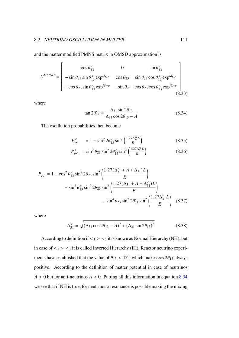
8.2. NEUTRINO OSCILLATION IN MATTER 111
and the matter modified PMNS matrix in OMSD approximation is
*$"(� =
cos \<13 0 sin \<13
− sin \23 sin \<13 exp8X�% cos \23 sin \23 cos \<13 exp8X�%
− cos \23 sin \<13 exp8X�% − sin \23 cos \23 cos \<13 exp8X�%
(8.33)
where
tan 2\<13 =Δ31 sin 2\13
Δ31 cos 2\13 − �(8.34)
The oscillation probabilities then become
%<44 = 1 − sin2 2\<13 sin2( 1.27Δ<31!
�
)(8.35)
%<`4 = sin2 \23 sin2 2\<13 sin2( 1.27Δ<31!
�
)(8.36)
%`` = 1 − cos2 \<13 sin2 2\23 sin2(1.27(Δ<31 + � + Δ31)!
�
)− sin2 \<13 sin2 2\23 sin2
(1.27(Δ31 + � − Δ<31)!�
)− sin4 \23 sin2 2\<13 sin2
(1.27Δ<31!
�
)(8.37)
where
Δ<31 =
√(Δ31 cos 2\13 − �)2 + (Δ31 sin 2\13)2 (8.38)
According to definition if<3 > <1 it is known asNormal Hierarchy (NH), but
in case of <1 > <3 it is called Inverted Hierarchy (IH). Reactor neutrino experi-
ments have established that the value of \13 < 45◦, which makes cos 2\13 always
positive. According to the definition of matter potential in case of neutrinos
� > 0 but for anti-neutrinos � < 0. Putting all this information in equation 8.34
we see that if NH is true, for neutrinos a resonance is possible making the mixing

112CHAPTER 8. NEUTRINO OSCILLATIONS IN VACUUM AND IN MATTER
angle \13 larger than its value in vacuum, and if IH is true for anti-neutrinos a res-
onance is possible making the mixing angle \13 larger than its value in vacuum.
But if NH is true then no resonance is present for anti-neutrinos and similarly for
neutrinos, in case of IH no resonance is present. These dissimilarities motivated
the design of INO. In presence of earth matter, the flux of neutrinos will get
modified if NH is true, and will be left unaltered for IH. But the opposite will be
observed in case of anti-neutrinos.
Chapter 9Matter vs Vacuum Oscillation in
Atmospheric Neutrinos
The pioneering water Cerenkov detectors, IMB [53, 54] and Kamiokande [55,
56], observed the up down asymmetry of atmospheric muon neutrinos and estab-
lished atmospheric neutrino anomaly. The next generation experiment, Super-
Kamiokande [57], measured the zenith angle dependence of atmospheric muon
and electron neutrinos and established atmospheric neutrino oscillations. The
initial analysis of Super-Kamiokande data was done using the hypothesis of
two flavor vacuum oscillations, which provided a good fit to the data. It also
has determined the magnitude of the corresponding mass-squared difference
|Δ0C< | ' 3 × 10⁻³ eV2 (but not its sign) and the mixing angle sin2 2\0C< ' 1.
This determination played an important role in the design of the long-baseline
accelerator neutrino experiments T2K [122] and NOaA [123].
Evidence for neutrino oscillations also came from solar neutrino experiments
[33, 34, 35, 36, 37, 38]. Analysis of the solar neutrino data yielded the result
113
114CHAPTER 9. MATTER VS VACUUM OSCILLATION IN ATMOSPHERIC
NEUTRINOS
ΔB>; ∼ 10−4 eV2 and sin2 \B>; ∼ 0.3. The three known light neutrino flavor states
[124] can mix to form three mass eigenstates with masses <1, <2 and <3. From
these, we can define two independent mass-square differences, Δ21 = <22 − <
21
and Δ31 = <23 − <
21. Without loss of generality, we can identify ΔB>; = Δ21 and
Δ0C< = Δ31 ≈ Δ32. The unitary mixing matrix, connecting the flavor eigenstates
to the mass eigenstates, is called the PMNS matrix [31, 32]. In a manner similar
to the quark mixing matrix [125, 126], it is parameterized in terms of three
mixing angles, \12, \13 and \23, and a CP violating phase X�%. The data from the
CHOOZ reactor neutrino experiment leads to the strong constraint \13 ≤ 10◦ [42,
43]. The smallness of this mixing angle implies that the solar and the atmospheric
neutrino anomalies can be analyzed as independent problems within the three
flavor oscillation framework [43]. It also leads to the identification \B>; ' \12
and \0C< ' \23.
The solar neutrinos, produced at the core of the sun, undergo forward elastic
scattering as they travel through the solar matter. This scattering leads to matter
effect [26, 127, 24], which modifies the solar electron neutrino survival probabil-
ity (%44). Super-Kamiokande [37] and SNO [38] havemeasured %44 as a function
of neutrino energy for � > 5 MeV and found it to be of a constant value ≈ 0.3.
SNO has also measured [38] the neutral current interaction rate of solar neutrinos
to be consistent with predictions of the standard solar model [13]. These results,
together with CHOOZ bound on \13, provide a 5 f evidence for the matter effects
in solar neutrinos [128]. The measurements of the 71�0 experiments [34, 35,
36] imply that %44 > 0.5 for neutrino energies � < 0.5 MeV. This increase in
%44 at lower energies can be explained only if Δ21 is positive.
The up going atmospheric neutrinos travel thousands of kilometers through
115
earth, during which they undergo forward elastic scattering with earth matter.
They also experience the matter effect [26, 127] which modifies their of survival
and oscillation probabilities. As in the case of the solar neutrinos, this modifi-
cation depends on the sign of the mass-square difference, which, in this case, is
Δ31. Given the different magnitudes of
• Δ21 and Δ31,
• the energies of solar and atmospheric neutrinos and
• the solar and earth matter densities,
the matter modification of atmospheric neutrino probabilities are of a different
mathematical form compared to their solar neutrino counterparts [129, 130].
An observation of these matter modifications can establish the sign of Δ31. A
number of studies [131, 58, 132, 133] considered matter modified oscillations
and explored the sensitivity of future atmospheric neutrino detectors to determine
whether hierarchy is NH or IH. Recently, SK experiment analyzed their data
using the hypothesis of matter modified oscillations. Their results indicate that
the vacuum oscillations are disfavored at 1.6 f only [134]. They prefer NH and
disfavor IH at 1.7 f.
At present, the most precise determination of |Δ31 | and sin2 2\23 comes from
the muon neutrino disappearance data of the accelerator neutrino experiments,
such as MINOS [135], T2K [136] and NOaA [137]. For baselines less than
1000 km, the matter effects lead to negligibly small changes in a`/a` survival
probabilities [138, 139]. Thus, the a`/a` disappearance data of accelerator
neutrino experiments lead to essentially the same values of |Δ31 | and sin2 2\23
116CHAPTER 9. MATTER VS VACUUM OSCILLATION IN ATMOSPHERIC
NEUTRINOS
for the three cases: (a) vacuum oscillations, (b) matter oscillations with NH and
(c) matter oscillations with IH. It is important to develop methods to make a
distinction between these three hypotheses. Without such a distinction, it will
be impossible to measure the CP violating phase X�% in neutrino oscillations
because matter effects mimic CP violation [140, 141]. In the present work, we
explore how this distinction can be made with future atmospheric neutrino data.
Disentangling the changes induced in the oscillation probabilities by the matter
effects and by X�% is non-trivial in general. In an atmospheric neutrino detector,
the interaction rate of a` (a`) depends on both the survival probability %`` (% ¯ ¯)
and the oscillation probability %4` (%4 ¯). However, it has been shown that the
sensitivity of this rate to matter effects does not depend on the value of X�%
[58]. Hence, this data can lead to a distinction between the three hypotheses,
independent of the value of X�%.
The a4/a4 appearance data in long-baseline accelerator neutrino experiments
is sensitive to matter effects [142, 143]. A precise measurement of the oscillation
probabilities, %`4 and % ¯4, in principle, can make a distinction among the three
possibilities. However, this data is also sensitive to X�% which at present is poorly
determined. Givenmeasured values of %`4 and % ¯4 can have three solutions [144,
145]:
• vacuum oscillations with X1�%
,
• NH matter oscillations with X2�%
and
• IH matter oscillations with X3�%
.
For each type of oscillating hypothesis, the value of X�% determined turns out
9.1. VACUUM VS. MATTER MODIFIED OSCILLATIONS 117
to be different. Since the determination of X�% is one of the important goals
of future long-baseline accelerator neutrino experiments, making a distinction
between the three hypotheses through independent data is crucial.
At present, the data of T2K and NOaA are analyzed using the matter modified
oscillation hypothesis with both NH and IH. T2K prefers NH and disfavors IH at
2 f [146]. It prefers X�% close to −c/2 for both NH and IH [147]. NOaA also
prefers NH, but it disfavors IH only at 1f [148]. In the case of NH, NOaA allows
the full range of X�% within 1 f, though it prefers −c/2 for IH. Very recently,
NOaA updated its results on hierarchy and X�% [149]. It still prefers NH with a
wide allowed range of X�% but also has a large 1 f allowed region for IH around
X�% ' −c/2. A combined analysis of the latest data of T2K and NOaA [150]
mildly prefers IH over NH (with a Δj2 = 1.8) whereas the combined analysis
of T2K and NOaA data along with that of Super-Kamiokande shows a mild
preference for NH over IH (with a Δj2 = 2.2). The combined data of T2K and
NOaA do not show any discrimination between vacuum and matter modified
oscillations with NH [151].
9.1 Vacuum vs. Matter Modified Oscillations
The mixing between the neutrino flavor eigenstates and the mass eigenstates is
given by a4
a`
ag
= *
a1
a2
a3
, (9.1)
118CHAPTER 9. MATTER VS VACUUM OSCILLATION IN ATMOSPHERIC
NEUTRINOS
where* is a 3 × 3 unitary PMNS matrix. It is parameterized as
* =
1 0 0
0 223 B23
0 −B23 223
213 0 B134−8X�%
0 1 0
−B1348X�% 0 213
212 B12 0
−B12 212 0
0 0 1
. (9.2)
For neutrino propagation in vacuum, the oscillation probabilities depend on
the six parameters: the two mass-squared differences, Δ21 = <22 − <
21 and
Δ31 = <23 − <
21, the three mixing angles and X�%. At present, Δ21, |Δ31 |, \12 and
\13 are measured quite precisely. In case of the third mixing angle, sin2 2\23 is
measured to be close to 1 but sin2 \23 has a rather large range of (0.4− 0.64). As
mentioned in the introduction, the sign of Δ31 is not known at present.
The effect of neutrino propagation in matter is parameterized by the Wolfen-
stein matter term � = 0.76× 10⁻⁴ d (8= 6</22) � (8= �4+) [26, 127]. Inclusion
of this matter term in neutrino evolution induces a change in the mass-square
differences and the mixing angles, and hence in the probabilities. In this work, it
has been studied how this change can be utilized to make a distinction between
vacuum and matter modified oscillations. This change depends on not only the
matter term but also on the sign of Δ31. Hence, both positive and negative values
of Δ31 have been considered.
First the difference between matter and vacuum oscillation probabilities for
two representative path-lengths for atmospheric neutrinos, ! = 5000 km and
! = 8000 km have been studied. Figure 9.1 shows the plots of neutrino and
anti-neutrino oscillation probabilities %4` and %4 ¯ and survival probabilities %``
and % ¯ ¯ for vacuum oscillations as well as for matter modified oscillations with
NH. The matter modified probabilities have been calculated numerically using
the code nuCraft [87], which uses the earth density profile of the PREM model
9.2. METHODOLOGY 119
[152]. From the expressions for the oscillation probabilities, it can be shown that
the probabilities for IH can be obtained via the relations %`` (��) = % ¯ ¯ (#�),
% ¯ ¯ (��) = %`` (#�), %`4 (��) = % ¯4 (#�) and %4 ¯ (��) = %4` (#�) [139].
From figure 9.1, it has been observed that, the matter effects increase the peak
value of %`4 from 0.05 to 0.2 (0.5) for L = 5000 (8000) km and these peak
values occur at nearly the same energy were %`` also peaks. Conservation of
probability implies that either %`` or %`g should decrease significantly. The
maximum of %`` generally coincide with the minimum of %`g and it can be
shown that the change in the value of %`g near its minimum is very small [139,
153]. Hence, most of the reduction in the probability occurs in %``. Thus,
%`` for matter, oscillations with NH is lower than %`` for vacuum oscillations
over a wide range of energies and path-lengths. But % ¯ ¯ is essentially the same
for both the cases. In the case of IH, the situation is reversed. Therefore, to
study the difference of vacuum oscillations from matter modified oscillations
of either sign, it is important to measure neutrino and anti-neutrino event rates
separately. In this work, the sensitivity of Iron Calorimeter (ICAL) at the India-
based Neutrino Observatory (INO) to make a distinction between vacuum and
matter modified oscillations using atmospheric neutrino data has been studied.
The charge identification capability of ICAL leads to a very good sensitivity for
this distinction [59].
9.2 Methodology
The atmospheric neutrinos consist of a`, a`, a4 and a4. The ICAL at INO is
a 50 kt magnetized iron calorimeter whose iron plates are interspersed with the
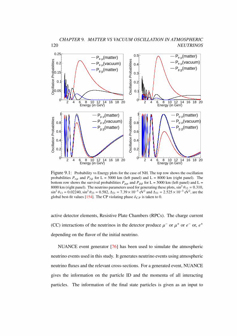
120CHAPTER 9. MATTER VS VACUUM OSCILLATION IN ATMOSPHERIC
NEUTRINOS
2 4 6 8 10 12 14 16 18 20Energy (in GeV)
0
0.05
0.1
0.15
0.2
0.25O
scill
atio
n P
roba
bilit
ies (matter)µe P
(vacuum)µe P(matter)µ eP
2 4 6 8 10 12 14 16 18 20Energy (in GeV)
0
0.1
0.2
0.3
0.4
0.5
Osc
illat
ion
Pro
babi
litie
s
(matter)µe P(vacuum)µe P(matter)µ eP
2 4 6 8 10 12 14 16 18 20Energy (in GeV)
0
0.2
0.4
0.6
0.8
1
Osc
illat
ion
Pro
babi
litie
s (matter)µ µP(vacuum)µ µP(matter)µ µP
2 4 6 8 10 12 14 16 18 20Energy (in GeV)
0
0.2
0.4
0.6
0.8
1
Osc
illat
ion
Pro
babi
litie
s
(matter)µ µP(vacuum)µ µP(matter)µ µP
Figure 9.1: Probability vs Energy plots for the case of NH. The top row shows the oscillationprobabilities %4` and %4 ¯ for L = 5000 km (left panel) and L = 8000 km (right panel). Thebottom row shows the survival probabilities %`` and % ¯ ¯ for L = 5000 km (left panel) and L =8000 km (right panel). The neutrino parameters used for generating these plots, sin2 \12 = 0.310,sin2 \13 = 0.02240, sin2 \23 = 0.582, Δ21 = 7.39× 10⁻⁵ eV2 and Δ31 = 2.525× 10⁻³ eV2, are theglobal best-fit values [154]. The CP violating phase X�% is taken to 0.
active detector elements, Resistive Plate Chambers (RPCs). The charge current
(CC) interactions of the neutrinos in the detector produce `− or `+ or 4− or, 4+
depending on the flavor of the initial neutrino.
NUANCE event generator [76] has been used to simulate the atmospheric
neutrino events used in this study. It generates neutrino events using atmospheric
neutrino fluxes and the relevant cross-sections. For a generated event, NUANCE
gives the information on the particle ID and the momenta of all interacting
particles. The information of the final state particles is given as an input to

9.2. METHODOLOGY 121
a GEANT4 simulator of ICAL. This simulator mimics the response of ICAL
and generates the electronic signals of the detector in the form of a hit bank
information as the output. A reconstruction program sifts through the hit bank
information of each event and tries to reconstruct a track. Electrons and positrons
in the final state produce a shower and quickly lose their energy. Identifying
such particles and reconstructing their energy is an extremely difficult problem.
Muons, being minimum ionizing particles, pass through many layers of iron,
leaving behind localized hits in the RPCs. Using this hit information, the track of
the muon can be reconstructed. Because of the magnetic field, this track will be
curved and the bending of the track is opposite for negative and positive muons.
Thus, ICAL can distinguish between the CC interactions of a` and a`. If a track
is reconstructed, the event is considered to be a CC interaction of a`/a`. The
charge, the momentum and the initial direction (cos \CA02: ), of a reconstructed
track, are also calculated from the track properties [84].
Un-oscillated atmospheric neutrino events for 500 years of exposure have
been generated using NUANCE. In generating these events, the neutrino fluxes
at Kamioka has been used as input along with ICAL geometry. The a`/a` CC
events are given as input to GEANT4 and the GEANT4 output is processed by
the reconstruction code. Events for which one or more tracks are reconstructed
are stored along with the charge, the momentum and the initial direction of the
track with the largest momentum. These track variables will be used later in the
analysis to bin the events. In the case of a4/a4 CC events, the electron/positron
are redefined to be `−/`+ and the events are processed through GEANT4 and
the reconstruction code. Once again the charge, the momentum and the initial
direction of the track with the largest momentum are stored. This redefinition
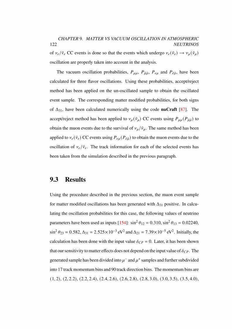
122CHAPTER 9. MATTER VS VACUUM OSCILLATION IN ATMOSPHERIC
NEUTRINOS
of a4/a4 CC events is done so that the events which undergo a4 (a4) → a` (a`)
oscillation are properly taken into account in the analysis.
The vacuum oscillation probabilities, %``, % ¯ ¯ , %4` and %4 ¯ , have been
calculated for three flavor oscillations. Using these probabilities, accept/reject
method has been applied on the un-oscillated sample to obtain the oscillated
event sample. The corresponding matter modified probabilities, for both signs
of Δ31, have been calculated numerically using the code nuCraft [87]. The
accept/reject method has been applied to a` (a`) CC events using %`` (% ¯ ¯) to
obtain the muon events due to the survival of a`/a`. The same method has been
applied to a4 (a4) CC events using %4` (%4 ¯) to obtain the muon events due to the
oscillation of a4/a4. The track information for each of the selected events has
been taken from the simulation described in the previous paragraph.
9.3 Results
Using the procedure described in the previous section, the muon event sample
for matter modified oscillations has been generated with Δ31 positive. In calcu-
lating the oscillation probabilities for this case, the following values of neutrino
parameters have been used as inputs [154]: sin2 \12 = 0.310, sin2 \13 = 0.02240,
sin2 \23 = 0.582, Δ31 = 2.525×10⁻³ eV2 andΔ21 = 7.39×10⁻⁵ eV2. Initially, the
calculation has been done with the input value X�% = 0. Later, it has been shown
that our sensitivity tomatter effects does not depend on the input value of X�%. The
generated sample has been divided into `− and `+ samples and further subdivided
into 17 trackmomentumbins and 90 track direction bins. Themomentumbins are
(1, 2), (2, 2.2), (2.2, 2.4), (2.4, 2.6), (2.6, 2.8), (2.8, 3.0), (3.0, 3.5), (3.5, 4.0),
9.3. RESULTS 123
(4.0, 4.5), (4.5, 5.0), (5.0, 6.0), (6.0, 7.5), (7.5, 9.0), (9.0, 11.0), (11.0, 14.0),
(14.0, 20.0), (20.0, 100.0). Only those events with track momentum greater than
1 GeV have been considered because such events lead to good track reconstruc-
tion. The signature of oscillations is very small for the down going events, and it
is almost impossible to reconstruct tracks of muons moving in horizontal direc-
tion. Therefore, only the up going events with cos \CA02: in the range (0.1, 1) have
been considered. Since ICAL can reconstruct the muon direction very accurately,
the above range have been subdivided into bins of equal width 0.01. Using this
procedure, two binned event samples, #30C0,`−
8 9and #30C0,`
+
8 9have been generated,
and treated as data. Here 8 refers to the track momentum bin and varies from 1
to 17 and 9 refers to cos \CA02: bin and varies from 1 to 90.
The vacuum oscillation has been considered as a hypothesis to be tested
against the data samples described above. Using the vacuum oscillation hypoth-
esis, two other event samples, #E02,`−
8 9and #E02,`
+
8 9, have been generated using
the same procedure described in the previous paragraph. In calculating the vac-
uum oscillation probabilities the five inputs, sin2 \12 = 0.310, sin2 \13 = 0.02240,
Δ31 = 2.525×10⁻³ eV2, Δ21 = 7.39×10⁻⁵ eV2 and X�% = 0, have been held fixed.
The test values of sin2 \23 have been varied in the range (0.4, 0.64). To quantify
the difference betweenmatter and vacuumoscillations,Δ#`−
8 9= #
E02,`−
8 9−#30C0,`
−
8 9
andΔ#`+
8 9= #
E02,`+
8 9−#30C0,`
+
8 9have been defined. In figure 9.2, Δ#`−
8= Σ 9Δ#
`−
8 9
and Δ#`+
8= Σ 9Δ#
`+
8 9as a function of track momentum have been plotted. Figure
9.3 gives the plots of Δ#`−
9= Σ8Δ#
`−
8 9and Δ#`+
9= Σ8Δ#
`+
8 9as a function of
track direction. It has been observed that Δ#`∓
8, in general, are positive because
the matter effects suppress the peak values of %`` and the magnitude of Δ#`−
8
is larger than that of Δ#`+
8for Δ31 positive. The situation is reversed when Δ31
124CHAPTER 9. MATTER VS VACUUM OSCILLATION IN ATMOSPHERIC
NEUTRINOS
is negative. This, of course, is a reflection of the fact that the matter effects are
more pronounced in %`` for positive value of Δ31 and in % ¯ ¯ for negative values
of Δ31. A similar pattern has been observed in Δ#`∓
9, for the same reasons.
11− 10− 9− 8− 7− 6− 5− 4− 3− 2− 1−Track momentum (in GeV)
100
200
300
400
500
600
700
800
- µ ij N∆ jΣ
=
i
- µ N∆
1 2 3 4 5 6 7 8 9 10 11Track momentum (in GeV)
0
50
100
150
200
250
+ µ ij N∆ jΣ
=
i
+ µ N∆
11− 10− 9− 8− 7− 6− 5− 4− 3− 2− 1−Track momentum (in GeV)
0
50
100
150
200
250
- µ ij N∆ jΣ
=
i
- µ N∆
1 2 3 4 5 6 7 8 9 10 11Track momentum (in GeV)
100
150
200
250
300
350
400
+ µ ij N∆ jΣ
=
i
+ µ N∆
Figure 9.2: The difference between the number of muon events for matter vs. vacuumoscillations (Δ#`
∓
8) as a function of track momentum. The plots in the left (right) panels are for
`− (`+) events. The plots in the top (bottom) panels are for Δ31 positive (negative).
The test event samples # C4BC,`−
8 9and # C4BC,`
+
8 9have been calculated as
#C4BC,`−/`+8 9
= #E02,`−/`+8 9
[1 + c:8 9b: ], (9.3)
where three systematic errors c:8 9(: = 1, 2, 3), each with its pull parameter, b:
have been introduced. The first of these is the systematic error in flux normaliza-
tion, which is independent of track momentum and track direction. The second
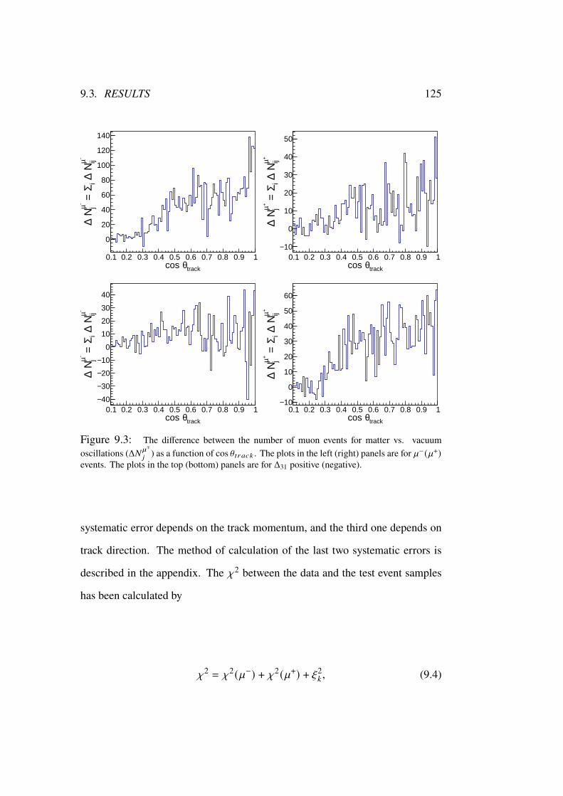
9.3. RESULTS 125
0.1 0.2 0.3 0.4 0.5 0.6 0.7 0.8 0.9 1
trackθcos
0
20
40
60
80
100
120
140
- µ ij N∆ iΣ
=
j
- µ N∆
0.1 0.2 0.3 0.4 0.5 0.6 0.7 0.8 0.9 1
trackθcos
10−
0
10
20
30
40
50
+ µ ij N∆ iΣ
=
j
+ µ N∆
0.1 0.2 0.3 0.4 0.5 0.6 0.7 0.8 0.9 1
trackθcos
40−
30−
20−
10−
0
10
20
30
40
- µ ij N∆ iΣ
=
j
- µ N∆
0.1 0.2 0.3 0.4 0.5 0.6 0.7 0.8 0.9 1
trackθcos
10−
0
10
20
30
40
50
60
+ µ ij N∆ iΣ
=
j
+ µ N∆
Figure 9.3: The difference between the number of muon events for matter vs. vacuumoscillations (Δ#`
∓
9) as a function of cos \CA02: . The plots in the left (right) panels are for `− (`+)
events. The plots in the top (bottom) panels are for Δ31 positive (negative).
systematic error depends on the track momentum, and the third one depends on
track direction. The method of calculation of the last two systematic errors is
described in the appendix. The j2 between the data and the test event samples
has been calculated by
j2 = j2(`−) + j2(`+) + b2: , (9.4)
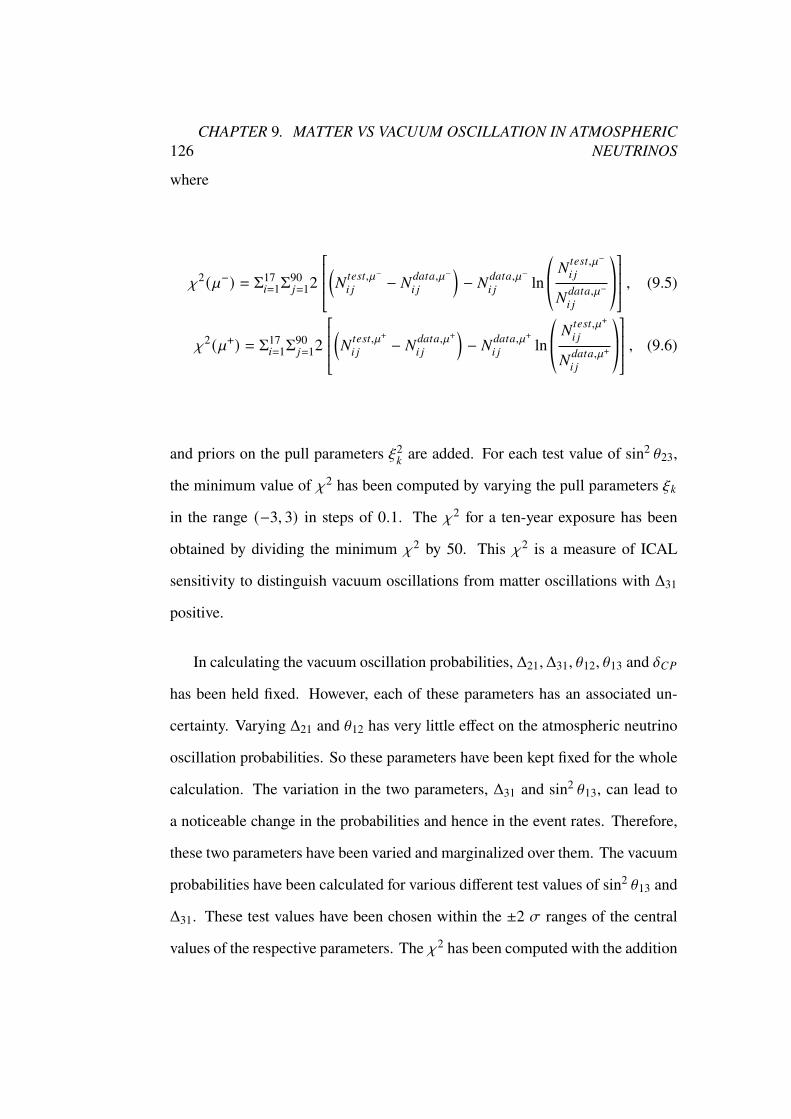
126CHAPTER 9. MATTER VS VACUUM OSCILLATION IN ATMOSPHERIC
NEUTRINOS
where
j2(`−) = Σ178=1Σ
909=12
(#C4BC,`−
8 9− #30C0,`
−
8 9
)− #30C0,`
−
8 9ln ©«
#C4BC,`−
8 9
#30C0,`−
8 9
ª®¬ , (9.5)
j2(`+) = Σ178=1Σ
909=12
(#C4BC,`+
8 9− #30C0,`
+
8 9
)− #30C0,`
+
8 9ln ©«
#C4BC,`+
8 9
#30C0,`+
8 9
ª®¬ , (9.6)
and priors on the pull parameters b2:are added. For each test value of sin2 \23,
the minimum value of j2 has been computed by varying the pull parameters b:
in the range (−3, 3) in steps of 0.1. The j2 for a ten-year exposure has been
obtained by dividing the minimum j2 by 50. This j2 is a measure of ICAL
sensitivity to distinguish vacuum oscillations from matter oscillations with Δ31
positive.
In calculating the vacuum oscillation probabilities, Δ21,Δ31, \12, \13 and X�%
has been held fixed. However, each of these parameters has an associated un-
certainty. Varying Δ21 and \12 has very little effect on the atmospheric neutrino
oscillation probabilities. So these parameters have been kept fixed for the whole
calculation. The variation in the two parameters, Δ31 and sin2 \13, can lead to
a noticeable change in the probabilities and hence in the event rates. Therefore,
these two parameters have been varied and marginalized over them. The vacuum
probabilities have been calculated for various different test values of sin2 \13 and
Δ31. These test values have been chosen within the ±2 f ranges of the central
values of the respective parameters. The j2 has been computed with the addition
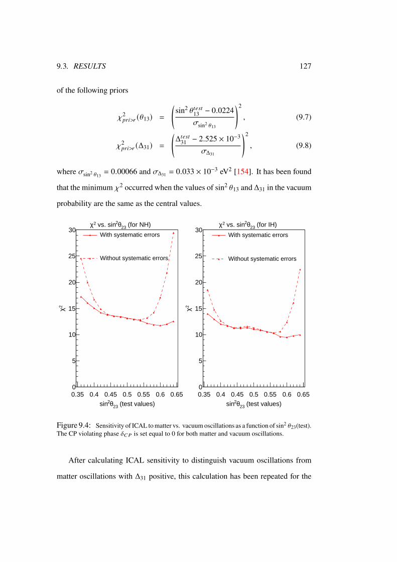
9.3. RESULTS 127
of the following priors
j2?A8>A (\13) =
(sin2 \C4BC13 − 0.0224
fsin2 \13
)2
, (9.7)
j2?A8>A (Δ31) =
(ΔC4BC31 − 2.525 × 10⁻³
fΔ31
)2
, (9.8)
where fsin2 \13= 0.00066 and fΔ31 = 0.033 × 10⁻³ eV2 [154]. It has been found
that the minimum j2 occurred when the values of sin2 \13 and Δ31 in the vacuum
probability are the same as the central values.
0.35 0.4 0.45 0.5 0.55 0.6 0.65
(test values)23θ2sin
0
5
10
15
20
25
30
2 χ
(for NH)23θ2 vs. sin2χWith systematic errors
Without systematic errors
0.35 0.4 0.45 0.5 0.55 0.6 0.65
(test values)23θ2sin
0
5
10
15
20
25
30
2 χ
(for IH)23θ2 vs. sin2χWith systematic errors
Without systematic errors
Figure 9.4: Sensitivity of ICAL tomatter vs. vacuumoscillations as a function of sin2 \23(test).The CP violating phase X�% is set equal to 0 for both matter and vacuum oscillations.
After calculating ICAL sensitivity to distinguish vacuum oscillations from
matter oscillations with Δ31 positive, this calculation has been repeated for the
128CHAPTER 9. MATTER VS VACUUM OSCILLATION IN ATMOSPHERIC
NEUTRINOS
case where Δ31 is negative. Our results are shown in figure 9.4 where the left
panel is for Δ31 positive and the right panel is for Δ31 negative. Each panel shows
the variation of j2 as a function of the test values of sin2 \23, without and with
the systematic errors. It has been observed that the j2 without systematic errors
is relatively flat for sin2 \23(test) in the range, (0.4, 0.6) but rises sharply outside
this range. This behavior can be explained by close examination of the difference
between the values of %`` near its minimum for the two cases of matter modified
oscillations and vacuum oscillations, as shown in figure 9.5. From this figure,
it can be noted that, values of %`` near the low energy minimum are very close
for matter modified oscillations with NH and for vacuum oscillations with test
values of sin2 \23 varying in the range (0.4, 0.6). But, for test value of sin2 \23
away from this range, these differences become bigger. And the contribution
from all these energy values leads to a significant rise in the j2. The uncertainty
in flux normalization, which is common to all the bins, is fairly large. Due to the
systematic error in the flux normalization, the j2 occurring due to the differences
near the %`` minima regions is drastically reduced, whereas the j2 occurring
due to the large difference near the %`` maxima regions is relatively unaffected.
Hence, the j2 with systematic errors is relatively flat with respect to all the test
values of sin2 \23.
It has been observed that j2<8=
= 11.8 for Δ31 positive and is 9.5 for Δ31
negative. Hence, ICAL can rule out vacuum oscillations at better than 3 f
confidence level, if the matter effects, as prescribed byWolfenstein [26, 127], are
present. This sensitivity is there for both the signs ofΔ31. The sensitivity obtained
is for the input values of sin2 \23 = 0.582 and sin2 2\13 ≈ 0.09, which are the
current best-fit values from the analysis of global data [154]. This sensitivity
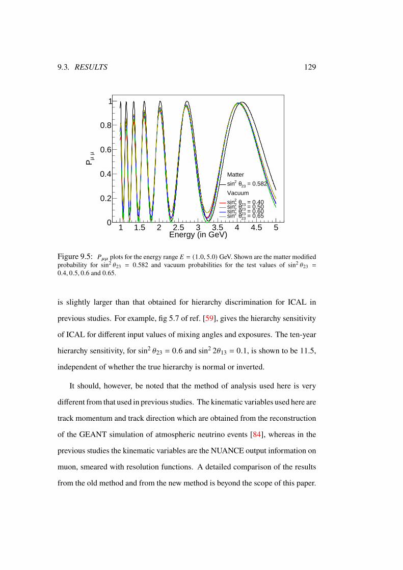
9.3. RESULTS 129
1 1.5 2 2.5 3 3.5 4 4.5 5Energy (in GeV)
0
0.2
0.4
0.6
0.8
1µ µ
P
Matter
= 0.58223θ 2sin
Vacuum
= 0.4023θ 2sin = 0.5023θ 2sin = 0.6023θ 2sin = 0.6523θ 2sin
Figure 9.5: %`` plots for the energy range � = (1.0, 5.0) GeV. Shown are the matter modifiedprobability for sin2 \23 = 0.582 and vacuum probabilities for the test values of sin2 \23 =
0.4, 0.5, 0.6 and 0.65.
is slightly larger than that obtained for hierarchy discrimination for ICAL in
previous studies. For example, fig 5.7 of ref. [59], gives the hierarchy sensitivity
of ICAL for different input values of mixing angles and exposures. The ten-year
hierarchy sensitivity, for sin2 \23 = 0.6 and sin2 2\13 = 0.1, is shown to be 11.5,
independent of whether the true hierarchy is normal or inverted.
It should, however, be noted that the method of analysis used here is very
different from that used in previous studies. The kinematic variables used here are
track momentum and track direction which are obtained from the reconstruction
of the GEANT simulation of atmospheric neutrino events [84], whereas in the
previous studies the kinematic variables are the NUANCE output information on
muon, smeared with resolution functions. A detailed comparison of the results
from the old method and from the new method is beyond the scope of this paper.
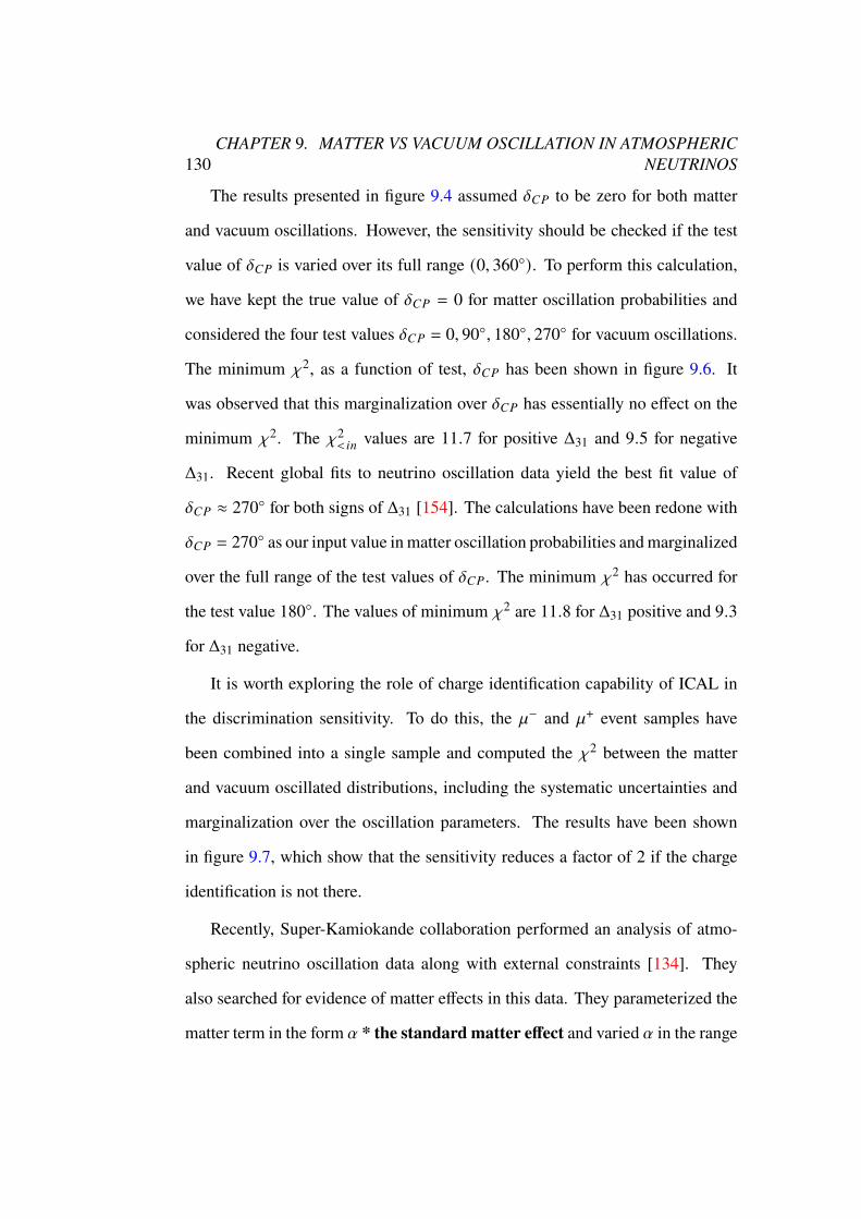
130CHAPTER 9. MATTER VS VACUUM OSCILLATION IN ATMOSPHERIC
NEUTRINOS
The results presented in figure 9.4 assumed X�% to be zero for both matter
and vacuum oscillations. However, the sensitivity should be checked if the test
value of X�% is varied over its full range (0, 360◦). To perform this calculation,
we have kept the true value of X�% = 0 for matter oscillation probabilities and
considered the four test values X�% = 0, 90◦, 180◦, 270◦ for vacuum oscillations.
The minimum j2, as a function of test, X�% has been shown in figure 9.6. It
was observed that this marginalization over X�% has essentially no effect on the
minimum j2. The j2<8=
values are 11.7 for positive Δ31 and 9.5 for negative
Δ31. Recent global fits to neutrino oscillation data yield the best fit value of
X�% ≈ 270◦ for both signs of Δ31 [154]. The calculations have been redone with
X�% = 270◦ as our input value inmatter oscillation probabilities andmarginalized
over the full range of the test values of X�%. The minimum j2 has occurred for
the test value 180◦. The values of minimum j2 are 11.8 for Δ31 positive and 9.3
for Δ31 negative.
It is worth exploring the role of charge identification capability of ICAL in
the discrimination sensitivity. To do this, the `− and `+ event samples have
been combined into a single sample and computed the j2 between the matter
and vacuum oscillated distributions, including the systematic uncertainties and
marginalization over the oscillation parameters. The results have been shown
in figure 9.7, which show that the sensitivity reduces a factor of 2 if the charge
identification is not there.
Recently, Super-Kamiokande collaboration performed an analysis of atmo-
spheric neutrino oscillation data along with external constraints [134]. They
also searched for evidence of matter effects in this data. They parameterized the
matter term in the form U * the standard matter effect and varied U in the range
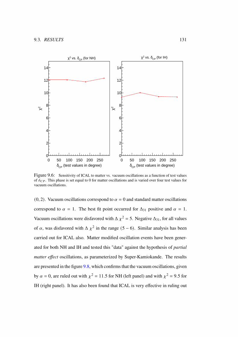
9.3. RESULTS 131
0 50 100 150 200 250 (test values in degree)CPδ
0
2
4
6
8
10
12
14
2 χ
(for NH)CPδ vs. 2χ
0 50 100 150 200 250 (test values in degree)CPδ
0
2
4
6
8
10
12
14
2 χ
(for IH)CPδ vs. 2χ
Figure 9.6: Sensitivity of ICAL to matter vs. vacuum oscillations as a function of test valuesof X�% . This phase is set equal to 0 for matter oscillations and is varied over four test values forvacuum oscillations.
(0, 2). Vacuum oscillations correspond to U = 0 and standard matter oscillations
correspond to U = 1. The best fit point occurred for Δ31 positive and U = 1.
Vacuum oscillations were disfavored with Δ j2 = 5. Negative Δ31, for all values
of U, was disfavored with Δ j2 in the range (5 − 6). Similar analysis has been
carried out for ICAL also. Matter modified oscillation events have been gener-
ated for both NH and IH and tested this "data" against the hypothesis of partial
matter effect oscillations, as parameterized by Super-Kamiokande. The results
are presented in the figure 9.8, which confirms that the vacuum oscillations, given
by U = 0, are ruled out with j2 = 11.5 for NH (left panel) and with j2 = 9.5 for
IH (right panel). It has also been found that ICAL is very effective in ruling out
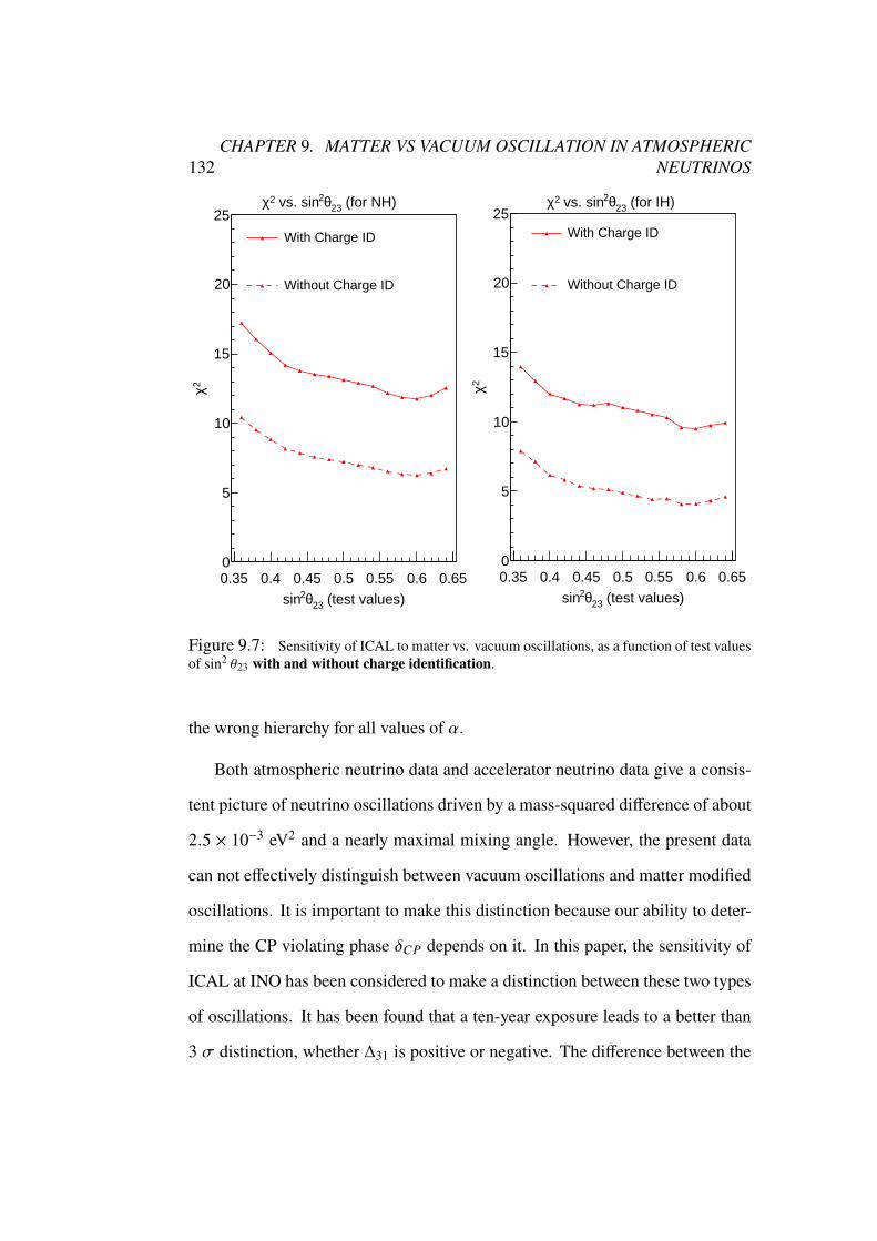
132CHAPTER 9. MATTER VS VACUUM OSCILLATION IN ATMOSPHERIC
NEUTRINOS
0.35 0.4 0.45 0.5 0.55 0.6 0.65
(test values)23θ2sin
0
5
10
15
20
25
2 χ (for NH)23θ2 vs. sin2χ
With Charge ID
Without Charge ID
0.35 0.4 0.45 0.5 0.55 0.6 0.65
(test values)23θ2sin
0
5
10
15
20
25
2 χ
(for IH)23θ2 vs. sin2χ
With Charge ID
Without Charge ID
Figure 9.7: Sensitivity of ICAL to matter vs. vacuum oscillations, as a function of test valuesof sin2 \23 with and without charge identification.
the wrong hierarchy for all values of U.
Both atmospheric neutrino data and accelerator neutrino data give a consis-
tent picture of neutrino oscillations driven by a mass-squared difference of about
2.5 × 10⁻³ eV2 and a nearly maximal mixing angle. However, the present data
can not effectively distinguish between vacuum oscillations and matter modified
oscillations. It is important to make this distinction because our ability to deter-
mine the CP violating phase X�% depends on it. In this paper, the sensitivity of
ICAL at INO has been considered to make a distinction between these two types
of oscillations. It has been found that a ten-year exposure leads to a better than
3 f distinction, whether Δ31 is positive or negative. The difference between the
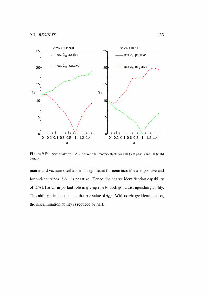
9.3. RESULTS 133
0 0.2 0.4 0.6 0.8 1 1.2 1.4α
0
5
10
15
20
25
2 χ
(for NH)α vs. 2χ
positive31∆test
negative31∆test
0 0.2 0.4 0.6 0.8 1 1.2 1.4α
0
5
10
15
20
25
2 χ
(for IH)α vs. 2χ
positive31∆test
negative31∆test
Figure 9.8: Sensitivity of ICAL to fractional matter effects for NH (left panel) and IH (rightpanel).
matter and vacuum oscillations is significant for neutrinos if Δ31 is positive and
for anti-neutrinos if Δ31 is negative. Hence, the charge identification capability
of ICAL has an important role in giving rise to such good distinguishing ability.
This ability is independent of the true value of X�%. With no charge identification,
the discrimination ability is reduced by half.

134CHAPTER 9. MATTER VS VACUUM OSCILLATION IN ATMOSPHERIC
NEUTRINOS
Chapter 10Neutrino Oscillation Parameter
Determination Using GEANT4
Reconstructed Event Information
One of the important physics goals of ICAL is to measure the oscillation param-
eters of atmospheric neutrinos with improved precision. The ability of ICAL to
reconstruct the muon momentum and direction with good accuracy plays an im-
portant role in achieving the above goal. The first analysis [61], which estimated
the precision in neutrino oscillation parameters possible at ICAL, used the NU-
ANCE output information of muon energy and direction. The detector resolution
was incorporated by means of smearing the energy and direction distributions
with the corresponding spreads. A later analysis [62] followed the same proce-
dure but used the hadron energy, defined to be the difference between neutrino
and muon energies given by NUANCE, as a third variable. It was shown that the
addition of a third variable led to a significant improvement in the precision of the
135
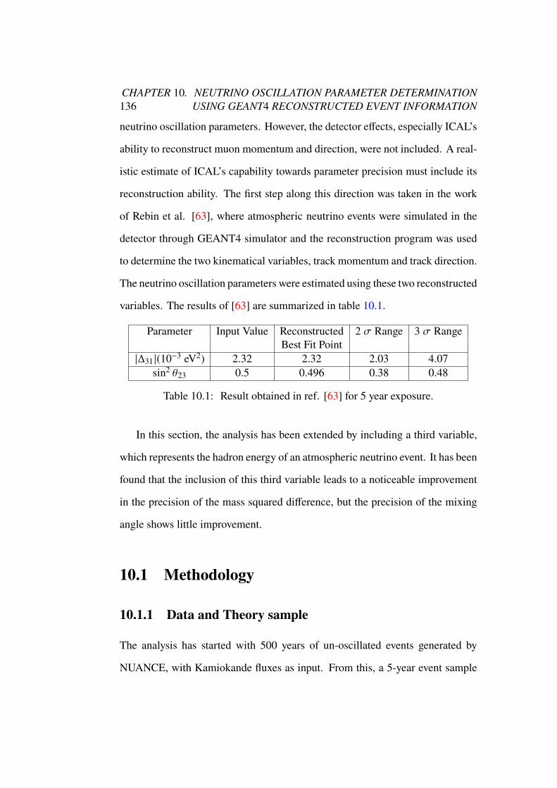
136CHAPTER 10. NEUTRINO OSCILLATION PARAMETER DETERMINATION
USING GEANT4 RECONSTRUCTED EVENT INFORMATION
neutrino oscillation parameters. However, the detector effects, especially ICAL’s
ability to reconstruct muon momentum and direction, were not included. A real-
istic estimate of ICAL’s capability towards parameter precision must include its
reconstruction ability. The first step along this direction was taken in the work
of Rebin et al. [63], where atmospheric neutrino events were simulated in the
detector through GEANT4 simulator and the reconstruction program was used
to determine the two kinematical variables, track momentum and track direction.
The neutrino oscillation parameters were estimated using these two reconstructed
variables. The results of [63] are summarized in table 10.1.
Parameter Input Value Reconstructed 2 f Range 3 f RangeBest Fit Point
|Δ31 |(10−3 eV2) 2.32 2.32 2.03 4.07sin2 \23 0.5 0.496 0.38 0.48
Table 10.1: Result obtained in ref. [63] for 5 year exposure.
In this section, the analysis has been extended by including a third variable,
which represents the hadron energy of an atmospheric neutrino event. It has been
found that the inclusion of this third variable leads to a noticeable improvement
in the precision of the mass squared difference, but the precision of the mixing
angle shows little improvement.
10.1 Methodology
10.1.1 Data and Theory sample
The analysis has started with 500 years of un-oscillated events generated by
NUANCE, with Kamiokande fluxes as input. From this, a 5-year event sample

10.1. METHODOLOGY 137
has been isolated. The oscillated event sample has been generated by using
accept/reject method on the above sample. The oscillation probabilities, %``
and % ¯ ¯ , have been calculated using the three flavor oscillation code nuCraft
[87]. The following values of neutrino oscillation parameters have been used as
inputs: sin2 \12 = 0.310, sin2 \13 = 0.02240, sin2 \23 = 0.5, Δ31 = 2.32 × 10⁻³
eV2, Δ21 = 7.39 × 10⁻⁵ eV2 and X�% = 0. The accept/reject method is applied to
a` (a`) CC events using %`` (% ¯ ¯) to obtain the muon events due to the survival
of a`/a`. The muon CC events occurring due to the oscillation of a4 (a4) are
negligibly small because sin2 \13 � 1. Hence, they are not included in this
analysis. This 5 year event sample is labeled data.
To calculate the corresponding theoretical event sample, with test values of
neutrino oscillation parameters, the following method has been followed. A test
value of |Δ31 | from the range (1, 5) × 10−34+2 and a test value of the sin2 \23
in the range (0, 1) have been chosen. The test values of |Δ31 | have been varied
systematically in steps of 0.2×10⁻³ eV2 in the range (1, 5)×10−3 eV2 and sin2 \23
in steps of 0.02 in the range (0, 1). The other neutrino oscillation parameters have
been kept fixed at the input values which were used to generate the data event
sample. The three flavor muon neutrino survival probabilities, %`` and % ¯ ¯ ,
have been calculated using the code nuCraft [87]. The rest 495 year un-oscillated
muon event sample has been converted into an oscillated event sample through
accept-reject method using the above probabilities.
138CHAPTER 10. NEUTRINO OSCILLATION PARAMETER DETERMINATION
USING GEANT4 RECONSTRUCTED EVENT INFORMATION
10.1.2 Variables for Analysis
Muons, being minimum ionizing particles, pass through many layers of iron,
leaving behind localized hits in the RPCs. Using this hit information, the track of
the muon can be reconstructed. Because of the magnetic field, this track will be
curved and the bending of the track is opposite for negative and positive muons.
Thus ICAL can distinguish between the CC interactions of a` and a`. If a track
has been reconstructed, the event has been considered to be a CC interaction
of a`/a`. The charge, the momentum and the initial direction (cos \CA02: ), of a
reconstructed track, are also calculated from the track properties [84]. Electrons,
positrons and photons lose their energy very quickly and leave no track. Pions
pass through a few layers, and it is difficult to construct a track for them unless
they are of very high energy. Baryons have very low kinetic energy and can pass
through one or two layers. Therefore, the hadrons produced in these reactions
leave a few (0− 10) scattered hits [81, 155]. Thus, the GEANT4 simulation of a
typical a`/a` CC event consists of a track and a few hadron hits.
Events for which one or more tracks have been reconstructed are stored along
with the charge, the momentum and the initial direction of the track with the
largest momentum. The leftover hits, that is the hits which are not used for track
reconstruction, have been labelled hadron hits. In dealing with the hadron hits,
the problem of ghost hits needs to be considered. If the actual hits occurred at
(G1, H2), (G2, H1) and (G3, H1) the simulation only tells us that the x-strips G1, G2, G3
and the y-strips H1, H2 are hit. This leads to the possibility of there being six hits,
three of which are ghost hits. This problem can be solved very simply by defining
the number of hadron hits to be the maximum of (number of x-strips, number of
10.1. METHODOLOGY 139
y-strips) with hits.
In this analysis, the following variables have been used, which are given as the
output of theGEANT4 simulator and the track reconstruction program. For about
90% of the events, only one track is reconstructed. Multitracks are reconstructed
for the other 10% of the events. For single track events, the variables used are (a)
the absolute value of the track momentum, (b) the direction of the track and (c)
the total number of non-track hits. For multitrack events, the variables used are
(a) the sum of absolute values of all the track momenta, (b) the direction of the
longest track and (c) the total number of non-track hits. This work concentrates
only in the parameters |Δ31 | and sin2 \23 but not inmatter effect. Therefore, a`/a`
CC events have been considered together, and the muon charge information has
not been used. This improves the statistics in each bin. The time information of
the events have not been used explicitly. The time stamps of hits, however, were
used by the reconstruction program in determining the track direction. Since the
co-ordinates of the hits are not relevant for this work, we need not worry about
the ghost hits.
10.1.3 Analysis Methods
The analysis have done using two different binning schemes. These schemes are
labeled as 2-Variable Analysis and 3-Variable Analysis:
• 2-Variable Analysis In this analysis method, the events have been binned
according to the modulus of their reconstructed track momentum and their
reconstructed track direction. For the events where more than one track
have been reconstructed, the trackmomentum and direction are those of the
140CHAPTER 10. NEUTRINO OSCILLATION PARAMETER DETERMINATION
USING GEANT4 RECONSTRUCTED EVENT INFORMATION
longest track. There are 10 momentum bins given by (0.1, 0.5), (0.5, 1.0),
(1.0, 1.5), (1.5, 2.0), (2.0, 2.5), (2.5, 3.0), (3.0, 5.0), (5.0, 10.0), (10.0, 20.0),
(20.0, 100.0). There are 40 direction bins spanning the range (−1, 1) in
steps of 0.05. This analysis uses 400 bins in the double differential distri-
bution of the two variables.
• 3-Variable Analysis This analysis method incorporates additional informa-
tion compared to two variable analysis method. We classified events into
four classes based on � , the total track momentum, and | cos \CA02: |, where
\CA02: is the direction of the longest reconstructed track. The four classes
are:
1. High energy, horizontal events with � > 10 GeV and | cos \CA02: | <
0.3, with 2 * 12 = 24 bins.
2. High energy, vertical events with � > 10 GeV and | cos \CA02: | >
0.3, with 2 * 28 = 56 bins.
3. Low energy, horizontal events with � < 10 GeV and | cos \CA02: | <
0.3, with 8 * 12 = 96 bins.
4. Low energy, vertical events with � < 10 GeV and | cos \CA02: | >
0.3, with 8 * 28 = 224 bins.
For atmospheric neutrinos, the number of events at high energies is small and
for ICAL the reconstruction ability for horizontal events is poor. Hence, the
number of events in each bin of the first three classes are too small to be further
subdivided based on non-track hits. Hence, the events in these 176 bins have been
binned only in the two variables � and cos \CA02: . Binning in the third variable,
10.1. METHODOLOGY 141
non-track hits, has been done only for the 224 bins of low energy, vertical events.
The bins used for the third variable are (0, 4), (5, 10) and > 10.
The data and the theory samples have been binned according to the scheme
described above. Each entry of the theory sample is divided by 99. Thus, the
theoretical prediction for a five-year muon event sample has been obtained if the
values of the oscillation parameters were equal to the chosen test values. Since
this theory event sample is generated by scaling a huge generated sample, it
is expected that the effect of fluctuations in each entry is negligibly small. On
the other hand, event number fluctuations are expected to distort both the track
momentum and track direction distributions in the data event sample.
10.1.4 Systematic Errors and j2Calculation
The theory event sample is calculated using standard inputs for atmospheric
neutrino fluxes and cross-sections. However, these inputs have uncertainties
associated with them. They have been taken into account as systematic errors
through the method of pulls. Usually three systematic errors are considered: a)
Normalization error, b) Energy dependent tilt error and c) Zenith angle depen-
dent error. The second and third errors are defined in terms of neutrino energy
and direction, respectively. But in our analysis, the variables used are track
momentum and direction. Hence, the systematic errors specified as functions
of neutrino energy and direction have to be transformed into functions of track
momentum and track direction. Following the method used in [156] the neutrino
energy dependent tilt error has been transformed to track momentum dependent
tilt error and neutrino direction dependent error has been transformed to recon-
142CHAPTER 10. NEUTRINO OSCILLATION PARAMETER DETERMINATION
USING GEANT4 RECONSTRUCTED EVENT INFORMATION
structed track direction dependent error. These two errors have been assumed to
be independent of each other. As described in the 3-variable binning scheme,
some events have been binned using the non-track hit information. An overall
5% systematic error has been considered for each of those bins. This has been
assumed to be independent of the momentum and direction of the longest track.
The method of pulls has been used to apply the systematic errors.
# C4BC8 9 :
has been defined as
# C4BC8 9 : = #Cℎ4>AH
8 9 :[1 + c;8 9 : ]b; , (10.1)
where b; is the pull variable for the systematic error ;, varied in the range -3 to
3 in step of 0.5. The pull coefficient c;8 9 :
is for the ;Cℎ systematic error. The
first three systematic errors are flux normalization dependent error(c=>A<), track
momentum dependent tilt error (cC8;C), track direction dependent error (c38A) and
the last one is systematic error (cℎ03) taken for each non-track hit information
bin in case of 3 variable analysis. A constant value of 0.2 has been assumed for
c=>A< and 0.05 for cℎ03 . The j2 between the data and test event samples is
j2 = Σ8Σ 9Σ:
[2
{(# C4BC8 9 : − #
30C08 9 :
)− #30C08 9 : ;=
(# C4BC8 9 :
#30C08 9 :
)}]+ b2
; , (10.2)
where the prior terms b2;have been added in the pull variables. This j2 is a
function of the test values of |Δ31 | and sin2 \23. For each pair of test values of
|Δ31 | and sin2 \23, j2 is computed, and the minimum j2 is evaluated. The test
values corresponding to minimum j2 are the best fit values of |Δ31 | and sin2 \23.
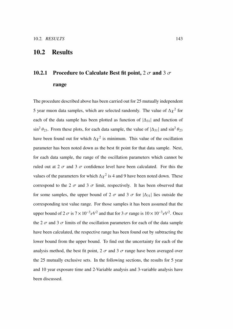
10.2. RESULTS 143
10.2 Results
10.2.1 Procedure to Calculate Best fit point, 2 f and 3 f
range
The procedure described above has been carried out for 25 mutually independent
5 year muon data samples, which are selected randomly. The value of Δj2 for
each of the data sample has been plotted as function of |Δ31 | and function of
sin2 \23. From these plots, for each data sample, the value of |Δ31 | and sin2 \23
have been found out for which Δj2 is minimum. This value of the oscillation
parameter has been noted down as the best fit point for that data sample. Next,
for each data sample, the range of the oscillation parameters which cannot be
ruled out at 2 f and 3 f confidence level have been calculated. For this the
values of the parameters for which Δj2 is 4 and 9 have been noted down. These
correspond to the 2 f and 3 f limit, respectively. It has been observed that
for some samples, the upper bound of 2 f and 3 f for |Δ31 | lies outside the
corresponding test value range. For those samples it has been assumed that the
upper bound of 2 f is 7× 10⁻³⁴+2 and that for 3 f range is 10× 10−34+2. Once
the 2 f and 3 f limits of the oscillation parameters for each of the data sample
have been calculated, the respective range has been found out by subtracting the
lower bound from the upper bound. To find out the uncertainty for each of the
analysis method, the best fit point, 2 f and 3 f range have been averaged over
the 25 mutually exclusive sets. In the following sections, the results for 5 year
and 10 year exposure time and 2-Variable analysis and 3-variable analysis have
been discussed.
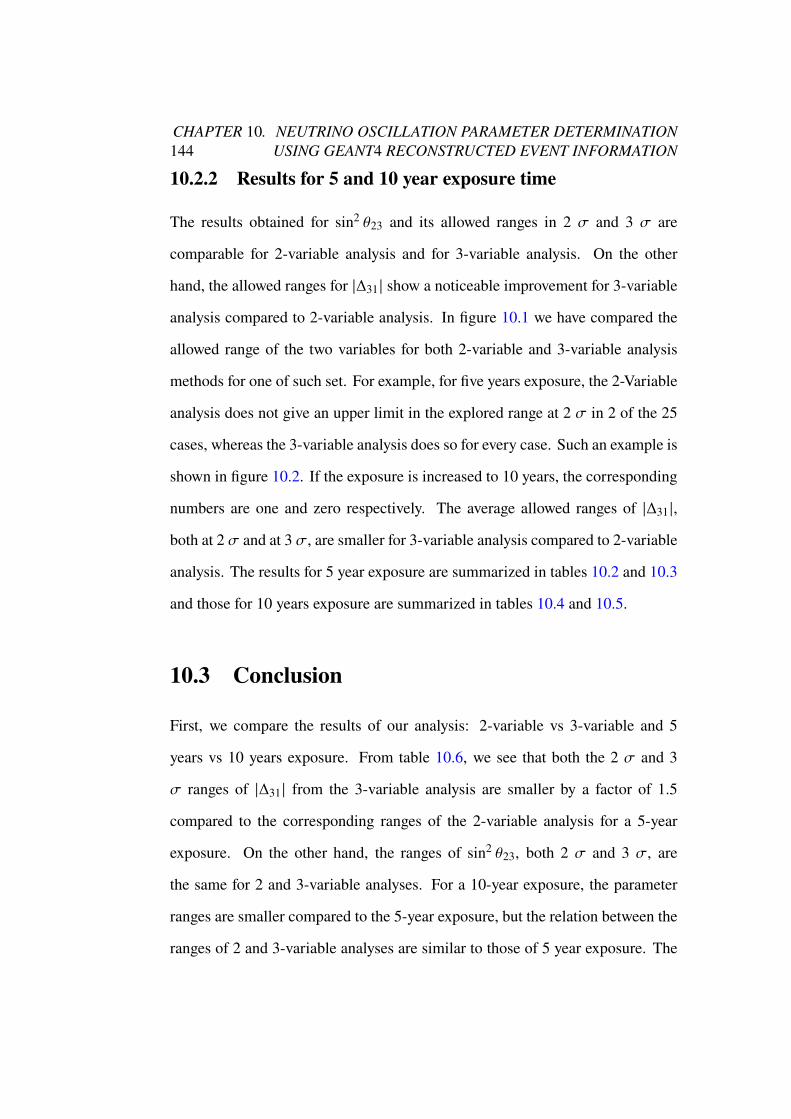
144CHAPTER 10. NEUTRINO OSCILLATION PARAMETER DETERMINATION
USING GEANT4 RECONSTRUCTED EVENT INFORMATION
10.2.2 Results for 5 and 10 year exposure time
The results obtained for sin2 \23 and its allowed ranges in 2 f and 3 f are
comparable for 2-variable analysis and for 3-variable analysis. On the other
hand, the allowed ranges for |Δ31 | show a noticeable improvement for 3-variable
analysis compared to 2-variable analysis. In figure 10.1 we have compared the
allowed range of the two variables for both 2-variable and 3-variable analysis
methods for one of such set. For example, for five years exposure, the 2-Variable
analysis does not give an upper limit in the explored range at 2 f in 2 of the 25
cases, whereas the 3-variable analysis does so for every case. Such an example is
shown in figure 10.2. If the exposure is increased to 10 years, the corresponding
numbers are one and zero respectively. The average allowed ranges of |Δ31 |,
both at 2 f and at 3 f, are smaller for 3-variable analysis compared to 2-variable
analysis. The results for 5 year exposure are summarized in tables 10.2 and 10.3
and those for 10 years exposure are summarized in tables 10.4 and 10.5.
10.3 Conclusion
First, we compare the results of our analysis: 2-variable vs 3-variable and 5
years vs 10 years exposure. From table 10.6, we see that both the 2 f and 3
f ranges of |Δ31 | from the 3-variable analysis are smaller by a factor of 1.5
compared to the corresponding ranges of the 2-variable analysis for a 5-year
exposure. On the other hand, the ranges of sin2 \23, both 2 f and 3 f, are
the same for 2 and 3-variable analyses. For a 10-year exposure, the parameter
ranges are smaller compared to the 5-year exposure, but the relation between the
ranges of 2 and 3-variable analyses are similar to those of 5 year exposure. The
10.3. CONCLUSION 145
0.3 0.4 0.5 0.6 0.7 0.823θ2sin
0
1
2
3
4
5
6
7
8
9
10
2 χ∆
23θ2 vs sin2χ∆ 23θ2 vs sin2χ∆
1 1.5 2 2.5 3 3.5 4 4.5 5)2 eV-3| (in 1031∆|
0
1
2
3
4
5
6
7
8
9
10
2 χ∆
|31∆ vs |2χ∆ |31∆ vs |2χ∆
((a)) Allowed ranges for 2-variable analysis method.
0.3 0.4 0.5 0.6 0.7 0.823θ2sin
0
1
2
3
4
5
6
7
8
9
10
2 χ∆
23θ2 vs sin2χ∆ 23θ2 vs sin2χ∆
1 1.5 2 2.5 3 3.5 4 4.5 5)2 eV-3| (in 1031∆|
0
1
2
3
4
5
6
7
8
9
10
2 χ∆
|31∆ vs |2χ∆ |31∆ vs |2χ∆
((b)) Allowed ranges for 3-variable analysis method.
Figure 10.1: Comparison between 2-variable and 3-variable analysis methodsfor one of the randomly selected sample set.
precision in |Δ31 | is greatly improved by the inclusion of the third variable. In
conclusion, we find that the precision in sin2 \23 improves by negligible amount
by the inclusion of the third variable. The precision on |Δ31 | on the other hand
improves by 32% when the third variable is included. The three variable analysis
method takes care of the energy of the other particles produced in the neutrino
146CHAPTER 10. NEUTRINO OSCILLATION PARAMETER DETERMINATION
USING GEANT4 RECONSTRUCTED EVENT INFORMATION
0.3 0.4 0.5 0.6 0.7 0.823θ2sin
0
1
2
3
4
5
6
7
8
9
10
2 χ∆23θ2 vs sin2χ∆ 23θ2 vs sin2χ∆
1 1.5 2 2.5 3 3.5 4 4.5 5)2 eV-3| (in 1031∆|
0
1
2
3
4
5
6
7
8
9
10
2 χ∆
|31∆ vs |2χ∆ |31∆ vs |2χ∆
((a)) Allowed ranges for 2-variable analysis method.
0.3 0.4 0.5 0.6 0.7 0.823θ2sin
0
1
2
3
4
5
6
7
8
9
10
2 χ∆
23θ2 vs sin2χ∆ 23θ2 vs sin2χ∆
1 1.5 2 2.5 3 3.5 4 4.5 5)2 eV-3| (in 1031∆|
0
1
2
3
4
5
6
7
8
9
10
2 χ∆
|31∆ vs |2χ∆ |31∆ vs |2χ∆
((b)) Allowed ranges for 3-variable analysis method.
Figure 10.2: Comparison between 2-variable and 3-variable analysis methodsfor one of the randomly selected sample set.
CC interactions. The parameter Δ31 being dependent on the value of L/Ea can
be measured more precisely if we have better reconstruction of neutrino energy
Ea. On the other hand, sin2 \23 is measured from the oscillation dip. The better
the dip is reconstructed, the more precise it will become. This has been observed
when we increased the exposure time to 10 years.
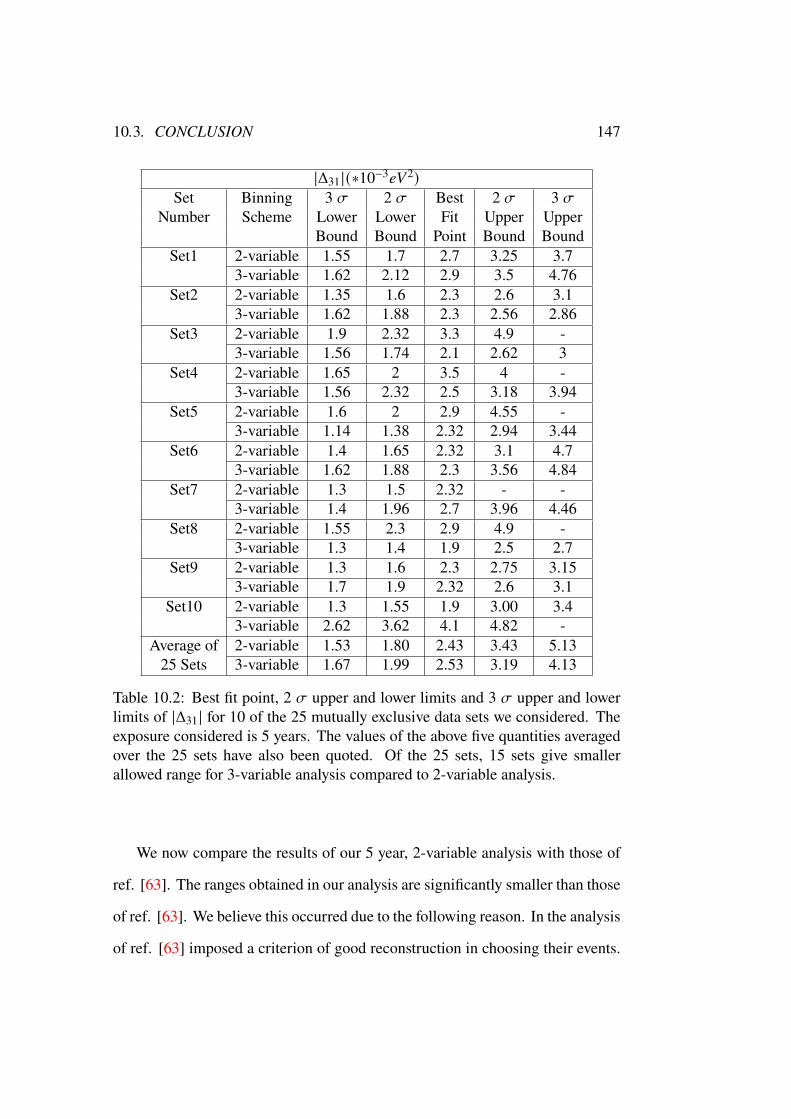
10.3. CONCLUSION 147
|Δ31 | (∗10−34+2)Set Binning 3 f 2 f Best 2 f 3 f
Number Scheme Lower Lower Fit Upper UpperBound Bound Point Bound Bound
Set1 2-variable 1.55 1.7 2.7 3.25 3.73-variable 1.62 2.12 2.9 3.5 4.76
Set2 2-variable 1.35 1.6 2.3 2.6 3.13-variable 1.62 1.88 2.3 2.56 2.86
Set3 2-variable 1.9 2.32 3.3 4.9 -3-variable 1.56 1.74 2.1 2.62 3
Set4 2-variable 1.65 2 3.5 4 -3-variable 1.56 2.32 2.5 3.18 3.94
Set5 2-variable 1.6 2 2.9 4.55 -3-variable 1.14 1.38 2.32 2.94 3.44
Set6 2-variable 1.4 1.65 2.32 3.1 4.73-variable 1.62 1.88 2.3 3.56 4.84
Set7 2-variable 1.3 1.5 2.32 - -3-variable 1.4 1.96 2.7 3.96 4.46
Set8 2-variable 1.55 2.3 2.9 4.9 -3-variable 1.3 1.4 1.9 2.5 2.7
Set9 2-variable 1.3 1.6 2.3 2.75 3.153-variable 1.7 1.9 2.32 2.6 3.1
Set10 2-variable 1.3 1.55 1.9 3.00 3.43-variable 2.62 3.62 4.1 4.82 -
Average of 2-variable 1.53 1.80 2.43 3.43 5.1325 Sets 3-variable 1.67 1.99 2.53 3.19 4.13
Table 10.2: Best fit point, 2 f upper and lower limits and 3 f upper and lowerlimits of |Δ31 | for 10 of the 25 mutually exclusive data sets we considered. Theexposure considered is 5 years. The values of the above five quantities averagedover the 25 sets have also been quoted. Of the 25 sets, 15 sets give smallerallowed range for 3-variable analysis compared to 2-variable analysis.
We now compare the results of our 5 year, 2-variable analysis with those of
ref. [63]. The ranges obtained in our analysis are significantly smaller than those
of ref. [63]. We believe this occurred due to the following reason. In the analysis
of ref. [63] imposed a criterion of good reconstruction in choosing their events.
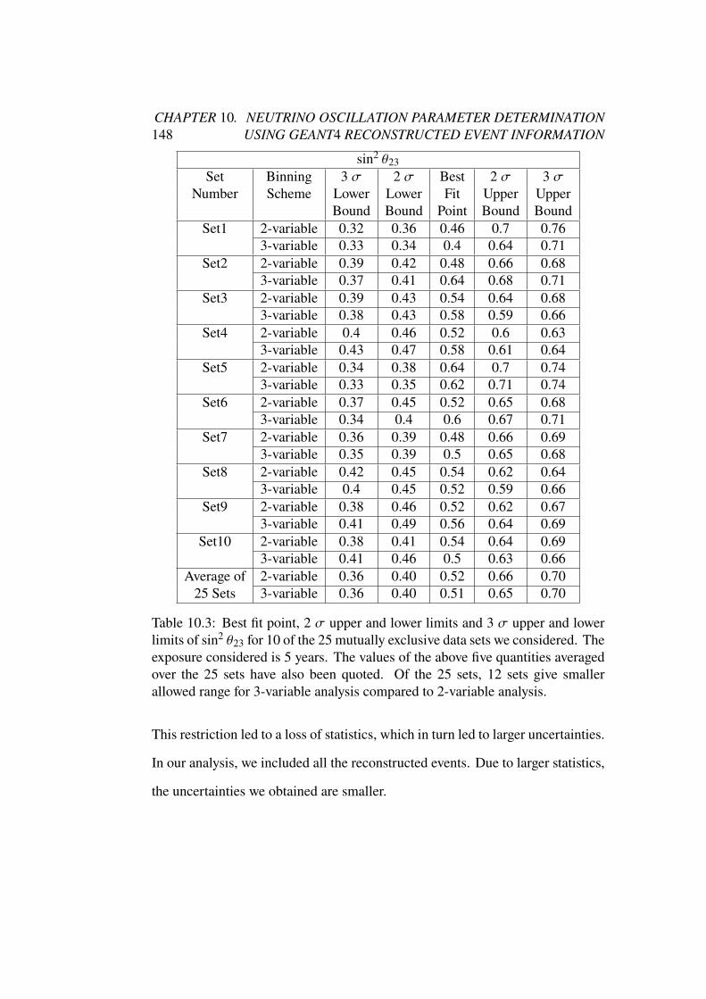
148CHAPTER 10. NEUTRINO OSCILLATION PARAMETER DETERMINATION
USING GEANT4 RECONSTRUCTED EVENT INFORMATION
sin2 \23Set Binning 3 f 2 f Best 2 f 3 f
Number Scheme Lower Lower Fit Upper UpperBound Bound Point Bound Bound
Set1 2-variable 0.32 0.36 0.46 0.7 0.763-variable 0.33 0.34 0.4 0.64 0.71
Set2 2-variable 0.39 0.42 0.48 0.66 0.683-variable 0.37 0.41 0.64 0.68 0.71
Set3 2-variable 0.39 0.43 0.54 0.64 0.683-variable 0.38 0.43 0.58 0.59 0.66
Set4 2-variable 0.4 0.46 0.52 0.6 0.633-variable 0.43 0.47 0.58 0.61 0.64
Set5 2-variable 0.34 0.38 0.64 0.7 0.743-variable 0.33 0.35 0.62 0.71 0.74
Set6 2-variable 0.37 0.45 0.52 0.65 0.683-variable 0.34 0.4 0.6 0.67 0.71
Set7 2-variable 0.36 0.39 0.48 0.66 0.693-variable 0.35 0.39 0.5 0.65 0.68
Set8 2-variable 0.42 0.45 0.54 0.62 0.643-variable 0.4 0.45 0.52 0.59 0.66
Set9 2-variable 0.38 0.46 0.52 0.62 0.673-variable 0.41 0.49 0.56 0.64 0.69
Set10 2-variable 0.38 0.41 0.54 0.64 0.693-variable 0.41 0.46 0.5 0.63 0.66
Average of 2-variable 0.36 0.40 0.52 0.66 0.7025 Sets 3-variable 0.36 0.40 0.51 0.65 0.70
Table 10.3: Best fit point, 2 f upper and lower limits and 3 f upper and lowerlimits of sin2 \23 for 10 of the 25 mutually exclusive data sets we considered. Theexposure considered is 5 years. The values of the above five quantities averagedover the 25 sets have also been quoted. Of the 25 sets, 12 sets give smallerallowed range for 3-variable analysis compared to 2-variable analysis.
This restriction led to a loss of statistics, which in turn led to larger uncertainties.
In our analysis, we included all the reconstructed events. Due to larger statistics,
the uncertainties we obtained are smaller.
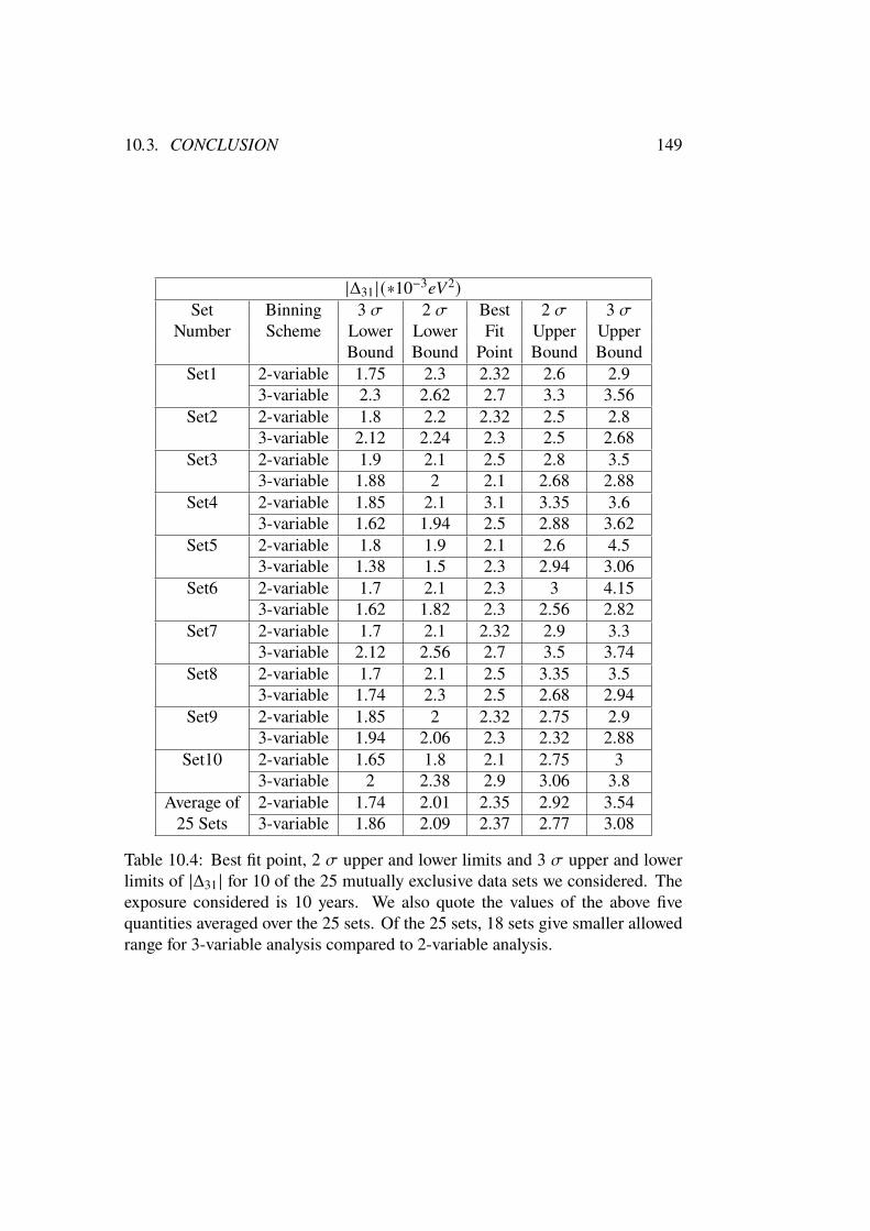
10.3. CONCLUSION 149
|Δ31 | (∗10−34+2)Set Binning 3 f 2 f Best 2 f 3 f
Number Scheme Lower Lower Fit Upper UpperBound Bound Point Bound Bound
Set1 2-variable 1.75 2.3 2.32 2.6 2.93-variable 2.3 2.62 2.7 3.3 3.56
Set2 2-variable 1.8 2.2 2.32 2.5 2.83-variable 2.12 2.24 2.3 2.5 2.68
Set3 2-variable 1.9 2.1 2.5 2.8 3.53-variable 1.88 2 2.1 2.68 2.88
Set4 2-variable 1.85 2.1 3.1 3.35 3.63-variable 1.62 1.94 2.5 2.88 3.62
Set5 2-variable 1.8 1.9 2.1 2.6 4.53-variable 1.38 1.5 2.3 2.94 3.06
Set6 2-variable 1.7 2.1 2.3 3 4.153-variable 1.62 1.82 2.3 2.56 2.82
Set7 2-variable 1.7 2.1 2.32 2.9 3.33-variable 2.12 2.56 2.7 3.5 3.74
Set8 2-variable 1.7 2.1 2.5 3.35 3.53-variable 1.74 2.3 2.5 2.68 2.94
Set9 2-variable 1.85 2 2.32 2.75 2.93-variable 1.94 2.06 2.3 2.32 2.88
Set10 2-variable 1.65 1.8 2.1 2.75 33-variable 2 2.38 2.9 3.06 3.8
Average of 2-variable 1.74 2.01 2.35 2.92 3.5425 Sets 3-variable 1.86 2.09 2.37 2.77 3.08
Table 10.4: Best fit point, 2 f upper and lower limits and 3 f upper and lowerlimits of |Δ31 | for 10 of the 25 mutually exclusive data sets we considered. Theexposure considered is 10 years. We also quote the values of the above fivequantities averaged over the 25 sets. Of the 25 sets, 18 sets give smaller allowedrange for 3-variable analysis compared to 2-variable analysis.

150CHAPTER 10. NEUTRINO OSCILLATION PARAMETER DETERMINATION
USING GEANT4 RECONSTRUCTED EVENT INFORMATION
sin2 \23Set Binning 3 f 2 f Best 2 f 3 f
Number Scheme Lower Lower Fit Upper UpperBound Bound Point Bound Bound
Set1 2-variable 0.42 0.48 0.5 0.56 0.643-variable 0.4 0.44 0.52 0.55 0.63
Set2 2-variable 0.45 0.48 0.54 0.59 0.643-variable 0.41 0.51 0.52 0.57 0.65
Set3 2-variable 0.41 0.43 0.56 0.64 0.673-variable 0.38 0.46 0.54 0.66 0.69
Set4 2-variable 0.46 0.51 0.54 0.57 0.613-variable 0.49 0.41 0.54 0.55 0.6
Set5 2-variable 0.39 0.44 0.62 0.63 0.673-variable 0.39 0.42 0.46 0.63 0.66
Set6 2-variable 0.41 0.54 0.58 0.64 0.663-variable 0.39 0.46 0.62 0.66 0.7
Set7 2-variable 0.4 0.46 0.5 0.62 0.673-variable 0.39 0.42 0.44 0.62 0.66
Set8 2-variable 0.4 0.43 0.54 0.59 0.643-variable 0.42 0.47 0.54 0.62 0.65
Set9 2-variable 0.44 0.49 0.52 0.61 0.663-variable 0.45 0.48 0.58 0.61 0.66
Set10 2-variable 0.42 0.45 0.56 0.61 0.653-variable 0.44 0.52 0.54 0.58 0.64
Average of 2-variable 0.39 0.43 0.52 0.62 0.6725 Sets 3-variable 0.40 0.45 0.52 0.62 0.66
Table 10.5: Best fit point, 2 f upper and lower limits and 3 f upper and lowerlimits of sin2 \23 for 10 of the 25 mutually exclusive data sets we considered.The exposure considered is 10 years. We also quote the values of the above fivequantities averaged over the 25 sets. Of the 25 sets, 13 sets give smaller allowedrange for 3-variable analysis compared to 2-variable analysis.
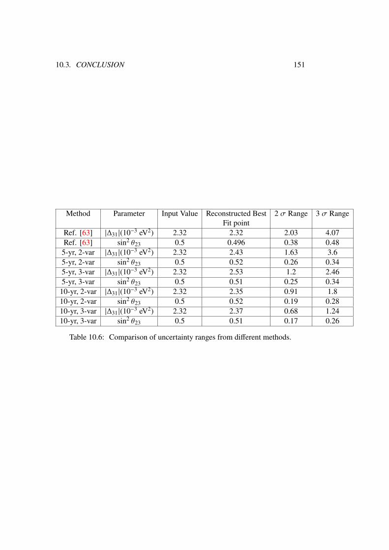
10.3. CONCLUSION 151
Method Parameter Input Value Reconstructed Best 2 f Range 3 f RangeFit point
Ref. [63] |Δ31 |(10−3 eV2) 2.32 2.32 2.03 4.07Ref. [63] sin2 \23 0.5 0.496 0.38 0.485-yr, 2-var |Δ31 |(10−3 eV2) 2.32 2.43 1.63 3.65-yr, 2-var sin2 \23 0.5 0.52 0.26 0.345-yr, 3-var |Δ31 |(10−3 eV2) 2.32 2.53 1.2 2.465-yr, 3-var sin2 \23 0.5 0.51 0.25 0.3410-yr, 2-var |Δ31 |(10−3 eV2) 2.32 2.35 0.91 1.810-yr, 2-var sin2 \23 0.5 0.52 0.19 0.2810-yr, 3-var |Δ31 |(10−3 eV2) 2.32 2.37 0.68 1.2410-yr, 3-var sin2 \23 0.5 0.51 0.17 0.26
Table 10.6: Comparison of uncertainty ranges from different methods.

152CHAPTER 10. NEUTRINO OSCILLATION PARAMETER DETERMINATION
USING GEANT4 RECONSTRUCTED EVENT INFORMATION
Chapter 11Conclusion and Outlook
ICAL is a 50 kt magnetized tracking calorimeter to be deployed in the un-
derground research facility of INO to study the long-standing neutrino mass-
hierarchy problem. The calorimeter will consist of three modules, each of
dimension 16 m × 16 m × 14.5 m, and will have 151 layers of 5.6 cm thick low
carbon iron slabs interspersed with a gap of 4 cm. The gaps will be occupied by
position sensitive gaseous detector, RPCs, the active component of the system.
Each module will be magnetized with electromagnets to produce a 1.3 T mag-
netic field in the active volume of the module. The setup will be used to track
the charged leptons created in the CC interactions of the muon neutrinos with
the iron nuclei using the RPCs. The magnetic field will bend the charged lep-
tons, in opposite directions depending on their polarity of the electrical charge,
leading to the separate measurements of neutrino and anti-neutrino event rates.
The ability of this experiment to make these separate measurements makes it a
unique detector.
The doctoral thesis deals with following projects in connection to the im-
153
154 CHAPTER 11. CONCLUSION AND OUTLOOK
provement of a few aspects of operation and performance of the ICAL detector.
• Exploration for alternative gas mixtures of the RPCs
• Discrimination of matter effect from vacuum oscillation in atmo-
spheric neutrino oscillation
• Determination of neutrino oscillation parameters using track and hit
information from GEANT4.
The outcome and conclusion for each of the projects are briefly described in the
following sections.
11.1 Exploration for alternative gas mixtures of
the RPCs
The goal of the ICAL experiment demands a spatial resolution ∼1 cm and time
resolution ∼ 1 ns [59] of the RPCs which can be achieved by operating the
detectors in avalanche mode with a gas mixture consisting of R134a(95.2%):i-
C4H10(4.5%):SF6(0.3%). High GWP of the gases R134a (1430) and SF6 (23900)
hasmade themixture unsuitable for long term use due to its negative impact on the
nature. This has motivated to a search for alternative eco-friendly gas mixtures
for avalanche mode operation of RPCs. To accomplish it, a predictive approach
has been adopted where a numerical framework has been developed to simulate
the RPC performance for a given gas mixture.
A hydro dynamical model has been developed to simulate the charge growth
in the RPC leading to either of the avalanche or streamer mode of operation. It
11.1. EXPLORATION FOR ALTERNATIVE GAS MIXTURES OF THE RPCS155
has been carried out on the platform of COMSOL Multiphysics using necessary
information of primary ionization and electron transport properties in the given
gas as produced by HEED and MAGBOLTZ. The characteristics of avalanche
and streamer events have been reproduced successfully using the model. The
precursor avalanche pulse before the streamer and presence of space charge field
equal to the applied electric field at the streamer head have been observed. The
model has been used to simulate the RPC performance in terms of efficiency
and streamer probability at different applied voltages for several gas mixtures.
The simulated detector responses for different gas mixtures have been compared
with several experiments [105, 106, 107] which has shown a close agreement
between the two, validating the simulation model. For further verification a
prototype of the glass RPC, to be used in the ICAL, has been fabricated and
a measurement of its efficiency and streamer probability has been carried out
at different applied voltages using the standard gas mixture of R134a(95.2%):i-
C4H10(4.5%):SF6(0.3%). The data have been analyzed with C++ based codes
developed for this purpose. The experimental results have been found to show
an agreement with the simulation. The successful validation of the numerical
model has led to its utilization in qualifying an eco-friendly, inexpensive and non-
flammable gas mixture of Ar(5%):CO2(60%):N2(35%) proposed for operating
the RPCs of the ICAL in avalanche mode.
Using the aforementioned simulation framework, the efficiency and streamer
probability of the RPC for this gas mixture have been calculated and compared
with the results of the standard R134a-based gas mixture. It has been observed
that for the proposed Ar-based gas mixture, the streamer probability is much
higher than the R134a-based gas mixture when the detector efficiency is more
156 CHAPTER 11. CONCLUSION AND OUTLOOK
than 90%. To address this problem, two approaches have been considered. One
of them is the classical approach of adding a small percentage of SF6 to reduce
the streamer probability. To keep the resultant GWP of this mixture within the
permissible limit, the SF6 has been allowed by a maximum amount of 0.5% of
the total gas volume. Addition of SF6 has improved the streamer probability of
the proposed Ar-based gas mixture, nevertheless it remains still larger than that
of the R134a-based mixture. The second option of reducing the threshold for
identifying valid signals has been found to yield better result. This approach
has improved the avalanche to streamer event ratio significantly and made the
streamer probability of the proposed Ar-based gas mixture comparable to the
standard R134a-based gas mixture without the SF6 component. The detector
response with the Ar-based gas mixtures has been compared with that measured
for other alternative gas mixtures, based on an allotropic form of tetrafluoro-
propene (HFO1234ze). From the comparison, it has been observed the proposed
eco-friendly Ar-based gas mixtures perform similarly to the HFO1234ze-based
gas mixtures without SF6. It could be noted that the proposed Ar-based gas
mixtures are also advantageous in terms of applying voltage due to the required
low operating voltage. When SF6 has been added to the HFO134ze-based gas
mixtures, they perform better than the Ar-based gas mixture, though their GWP
cross the permissible limit. In case of reduced threshold, the Ar-based gas
mixture has been found to behave comparably with the HFO1234ze-based gas
mixtures with SF6. Therefore, the present study has demonstrated that the gas
mixture of Ar(5%):CO2(60%):N2(35%), which is an eco-friendly and safe mix-
ture for the environment can be considered as a potential substitute of the standard
R134a(95.2%):i-C4H10(4.5%):SF6(0.3%) mixture for avalanche mode operation
11.2. DISCRIMINATION OF MATTER EFFECT FROM VACUUMOSCILLATION IN ATMOSPHERIC NEUTRINO OSCILLATION 157
of the RPCs in the ICAL. However, it requires lowering of the electronic threshold
to reduce the streamer probability at higher efficiency, which on the other hand
may allow electronic noise to increase. It calls for detailed investigation in future
with experimental measurements to validate the numerical findings and explore
the possibilities to alleviate the issue of noise.
11.2 Discrimination of matter effect from vacuum
oscillation in atmospheric neutrino oscillation
Different solar neutrino experiments have established matter effect in neutrino
oscillation beyond any ambiguity. But all the atmospheric and long-baseline neu-
trino experiments have been found to follow the hypothesis of vacuum oscillation.
Also, the oscillation parameter measurement assuming matter and vacuum hy-
potheses has returned similar results. The recent analysis by SK collaboration
could discriminate matter effect in neutrino oscillation from vacuum hypothesis
with a significance of 1.6 f. Though the long-baseline experiments, like T2K,
NOaA can measure the a4/a4 appearance data which can establish the Earth
matter effect in neutrino oscillation, it is also sensitive to CP violating phase X�%
which can mimic the Earth matter effect. So, to disentangle the Earth matter
effect from the effect of CP violation and for an accurate measurement of the CP
violating phase, different experiments should establish the Earth matter effect in
neutrino oscillations. In this work it has been shown that with 10 years of data,
the ICAL can discriminate the Earth matter effect in neutrino oscillation from
vacuum oscillation hypothesis with 3 f significance irrespective of the neutrino

158 CHAPTER 11. CONCLUSION AND OUTLOOK
mass hierarchy or the value of the CP violating phase. The difference between
the matter and vacuum oscillation is significant for neutrinos if Δ<231 is positive
and for anti-neutrinos if Δ<231 is negative. So, the charge identification capability
of ICAL plays a huge role in this regard. If charge identification capability is not
there, ICAL can discriminate these two hypotheses with much less significance.
11.3 Determination of neutrino oscillation
parameters using track and hit information
from GEANT4
This work is related to the development of an analysis method to improve the
precision of neutrino oscillation parameter measurement with the ICAL. The
work has incorporated hadron and muon information to reconstruct the parent
neutrino. This information has been simulated using the GEANT4 based event
by event reconstruction algorithm developed for the ICAL. To incorporate the
effect of fluctuation in data that ICAL will observe in a 5 year or 10 year long
operation, the analysis method has used 25 randomly selected mutually exclusive
sets of simulated events for 5 year and 10 year exposure time respectively. The
oscillation parameters have been measured using two analysis methods as follows
• 2-variable analysis method, the conventional method using only muon
information that has been followed by Rebin et al. [63].
• 3-variable analysis method, the newly developed method incorporating
information of hadrons along with muons.
11.3. DETERMINATION OF NEUTRINO OSCILLATION PARAMETERSUSING TRACK AND HIT INFORMATION FROM GEANT4 159
It has been found that the fluctuation present in 5 year long ICAL run affects
the parameter measurement using 2-variable analysis method severely. With this
method, for quite a few of the sets, the 3 f upper bound for Δ31 has been found
to be lying outside the test value range of the said parameter. This has been
absent in case of 3-variable analysis method, which has improved the precision
of Δ31 measurement. But the results for sin2 \23 with these two analysis methods
have been found to be comparable with each other. When the exposure time has
been increased to 10 years, the number of data sets, for which 3 f upper bound
lies outside the test value range of Δ31, has reduced to one. However, no such
set has been observed in case of 3-variable analysis method. The precision for
sin2 \23 has improved for both the analysis methods with the increase in exposure
time, but remained comparable to each other. In conclusion, it can be said that
the 3-variable analysis method has been found to be better than the traditional
2-variable analysis method to improve the precision of Δ31 measurement. As it
has been observed that the number of reconstructed events with tracks and hadron
information has improved the precision, inclusion of machine learning methods
may be found useful.

160 CHAPTER 11. CONCLUSION AND OUTLOOK
Appendix AAppendix
A.1 Calculation of systematic errors
In the appendix, we describe the method by which we computed the two sys-
tematic errors, one of which depends on track momentum and the other on
track direction. Usually, the atmospheric neutrino fluxes are listed with three
systematic errors:
• Normalization error (common for all the bins)
• Tilt error (which depends on neutrino energy)
• Direction error (which depends on neutrino direction).
The normalization error on neutrino flux translates directly into the normalization
of the neutrino event rates in all bins and hence is independent of trackmomentum
and track direction also. The tilt error is taken to be cC8;C8 9= cC8;C
8= 0.05∗ ;=(�a/2)
and the direction error is assumed to be c=D38A8 9
= c=D38A9
= 0.05 ∗ | cos(\a) | [157],
where �a and \a are the energy and the zenith angle of the neutrino respectively.
161
162 APPENDIX A. APPENDIX
We outline the procedure for the construction of the transfer matrices which
convert the systematic errors in neutrino energy and direction to systematic
errors in track momentum and direction. To keep the calculations tractable, we
make two simplifying assumptions. We assume that track momentum dependent
systematic error depends only on neutrino energy dependent systematic error and
not on neutrino direction dependent systematic error. In computing this error, we
consider only the modulus of the track momentum and do not make a distinction
between the charges. Similarly wewill also assume that track direction dependent
systematic error depends only on the neutrino direction dependent systematic
error and not on the neutrino energy dependent systematic error. Here also,
we consider only modulus of the cosine of the zenith angle and do not make a
distinction between up-going and down-going particles.
From the simulation of 500 years of un-oscillated events, the a`-CC and a`-
CC events with a well reconstructed track are chosen. These events are classified
into ten bins of �a and the event numbers are labeled #1, #2, ... #10. The events
in the set #1 are further classified into ten bins based on the modulus of track
momentum. These event numbers are called �11, �21, ... �10,1, each of which is
divided by #1 to get a set of ten fractions 011, 021, ... 010,1. These ten fractions
form the first column of the transfer matrix 0. We repeat this procedure for each
of #2, #3, ..., #10 to construct the rest of the columns of the 10 × 10 matrix 0.

A.1. CALCULATION OF SYSTEMATIC ERRORS 163
Now we can write a matrix equation of the form
)1
)2
.
.
)10
=
011 012 . . 01,10
021 022 . . 02,10
. . . . .
. . . . .
010,1 010,2 . . 010,10
#1
#2
.
.
#10
. (A.1)
The numbers in the column matrix on the LHS, )1, )2, ..., )10 are the number
of events distributed into ten bins in the modulus of track momentum. Thus, we
construct the transfer matrix which converts the distribution of events in neutrino
energy into distribution of events in the magnitude of the track momentum.
We assume that the systematic errors in #1 (cC8;C1 ) is independent of the sys-
tematic error in #2 (cC8;C2 ) and all other systematic errors in other # 9s. Therefore
the systematic error in )1 (cCA:<<1 ) will be
cCA:<<1 =
√(011 ∗ cC8;C1 )2 + (012 ∗ cC8;C2 )2 + ... + (01,10 ∗ cC8;C10 )2. (A.2)
Similarly the systematic error in )2 will be
cCA:<<2 =
√(021 ∗ cC8;C1 )2 + (022 ∗ cC8;C2 )2 + ... + (02,10 ∗ cC8;C10 )2 (A.3)
This way we can compute all the ten cC8;C8
for each )8 (8 = 1, 2, ..., 10).
Similarly we can compute the transfer matrix and cCA:38A9
for converting the
systematic error in neutrino direction into systematic error in | cos \C02A: |. Once
these two sets of numbers, cCA:<<8
and cCA:38A9
are ready, we can write the theoret-
ical number of events (including the systematic errors), binned in |CA:<< | and
cos(\CA: ) to be
# Cℎ8 9 = #08 9
[1 + 0.2 ∗ b=>A< + cCA:<<8 bCA:<< + cCA:38A9 bCA:38A
], (A.4)

164 APPENDIX A. APPENDIX
where #08 9is the number of theoretically expected events in the 8 9 th bin, according
to CA:<< and cos(\CA02: ). This expression for # Cℎ8 9 is used to calculate j2.

Bibliography
[1] https://en.wikipedia.org/wiki/Standard_Model.
[2] Matthew D. Schwartz. Quantum Field Theory and The Standard Model.
Cambridge University Press, 2014. isbn: 9781107034730.
[3] Georges Aad et al. “Observation of a new particle in the search for the
Standard Model Higgs boson with the ATLAS detector at the LHC”. In:
Phys. Lett. B 716 (2012), pp. 1–29. doi: 10.1016/j.physletb.2012.08.020.
arXiv: 1207.7214 [hep-ex].
[4] D. Decamp et al. “Determination of the Number of Light Neutrino
Species”. In: Phys. Lett. B 231 (1989), pp. 519–529. doi: 10.1016/0370-
2693(89)90704-1.
[5] S. Schael et al. “Precision electroweak measurements on the / reso-
nance”. In: Phys. Rept. 427 (2006), pp. 257–454. doi: 10.1016/j.physrep.
2005.12.006. arXiv: hep-ex/0509008.
[6] P. Aarnio et al. “Measurement of the Mass and Width of the /0 Particle
from Multi - Hadronic Final States Produced in 4+4− Annihilations”. In:
165
166 BIBLIOGRAPHY
Phys. Lett. B 231 (1989), pp. 539–547. doi: 10.1016/0370-2693(89)
90706-5.
[7] B. Adeva et al. “A Determination of the Properties of the Neutral In-
termediate Vector Boson /0”. In: Phys. Lett. B 231 (1989), p. 509. doi:
10.1016/0370-2693(89)90703-X.
[8] M. Z. Akrawy et al. “Measurement of the /0 Mass and Width with the
OPAL Detector at LEP”. In: Phys. Lett. B 231 (1989), pp. 530–538. doi:
10.1016/0370-2693(89)90705-3.
[9] Carlo Giunti and Chung W. Kim. Fundamentals of Neutrino Physics and
Astrophysics. Oxford University Press, 2007. isbn: 9780198508717.
[10] C. L. Cowan et al. “Detection of the free neutrino: A Confirmation”. In:
Science 124 (1956), pp. 103–104. doi: 10.1126/science.124.3212.103.
[11] G. Danby et al. “Observation of High-Energy Neutrino Reactions and
the Existence of Two Kinds of Neutrinos”. In: Phys. Rev. Lett. 9 (1962),
pp. 36–44. doi: 10.1103/PhysRevLett.9.36.
[12] K. Kodama et al. “Observation of tau neutrino interactions”. In: Phys.
Lett. B 504 (2001), pp. 218–224. doi: 10.1016/S0370-2693(01)00307-0.
arXiv: hep-ex/0012035.
[13] John N. Bahcall and M. H. Pinsonneault. “What do we (not) know the-
oretically about solar neutrino fluxes?” In: Phys. Rev. Lett. 92 (2004),
p. 121301. doi: 10 . 1103 / PhysRevLett . 92 . 121301. arXiv: astro - ph /
0402114.
BIBLIOGRAPHY 167
[14] John N. Bahcall. Neutrino Astrophysics. Cambridge University Press,
1989. isbn: 9780521379755.
[15] Raymond Davis Jr., Don S. Harmer, and Kenneth C. Hoffman. “Search
for neutrinos from the sun”. In: Phys. Rev. Lett. 20 (1968), pp. 1205–
1209. doi: 10.1103/PhysRevLett.20.1205.
[16] B. Pontecorvo. “Neutrino Experiments and the Problem of Conservation
of Leptonic Charge”. In: Zh. Eksp. Teor. Fiz. 53 (1967), pp. 1717–1725.
[17] L. B. Okun, M. B. Voloshin, and M. I. Vysotsky. “Neutrino Electrody-
namics and Possible Effects for Solar Neutrinos”. In: Sov. Phys. JETP 64
(1986), pp. 446–452.
[18] Arturo Cisneros. “Effect of neutrino magnetic moment on solar neutrino
observations”. In: Astrophys. Space Sci. 10 (1971), pp. 87–92. doi: 10.
1007/BF00654607.
[19] Z.G. Berezhiani and M.I. Vysotsky. “Neutrino decay in matter”. In:
Physics Letters B 199.2 (1987), pp. 281–285. issn: 0370-2693. doi:
https://doi.org/10.1016/0370-2693(87)91375-X. url: https://www.
sciencedirect.com/science/article/pii/037026938791375X.
[20] John N. Bahcall, N. Cabibbo, and A. Yahil. “Are neutrinos stable par-
ticles?” In: Phys. Rev. Lett. 28 (1972), pp. 316–318. doi: 10 . 1103 /
PhysRevLett.28.316.
[21] Sheldon L. Glashow and Lawrence M. Krauss. ““Just so” neutrino os-
cillations”. In: Physics Letters B 190.1 (1987), pp. 199–207. issn: 0370-
2693. doi: https : / / doi . org / 10 . 1016 / 0370 - 2693(87 ) 90867 - 7. url:
https://www.sciencedirect.com/science/article/pii/0370269387908677.
168 BIBLIOGRAPHY
[22] Livia Ludhova. “Experimental data on solar neutrinos”. In: Eur. Phys. J.
A 52.4 (2016), p. 82. doi: 10.1140/epja/i2016-16082-5.
[23] S. P. Mikheyev and A. Yu. Smirnov. “Resonance Amplification of Oscil-
lations in Matter and Spectroscopy of Solar Neutrinos”. In: Sov. J. Nucl.
Phys. 42 (1985), pp. 913–917.
[24] S. P. Mikheev and A. Yu. Smirnov. “Resonant amplification of neutrino
oscillations in matter and solar neutrino spectroscopy”. In: Nuovo Cim.
C 9 (1986), pp. 17–26. doi: 10.1007/BF02508049.
[25] S. P. Mikheev and A. Yu. Smirnov. “Resonance Oscillations of Neutrinos
in Matter”. In: Sov. Phys. Usp. 30 (1987), pp. 759–790. doi: 10.1070/
PU1987v030n09ABEH002961.
[26] L. Wolfenstein. “Neutrino Oscillations in Matter”. In: Phys. Rev. D 17
(1978), pp. 2369–2374. doi: 10.1103/PhysRevD.17.2369.
[27] John N. Bahcall, P. I. Krastev, and A. Yu. Smirnov. “Is large mixing
angle MSW the solution of the solar neutrino problems?” In: Phys. Rev.
D 60 (1999), p. 093001. doi: 10 .1103/PhysRevD.60.093001. arXiv:
hep-ph/9905220.
[28] AlanW. P. Poon et al. “Neutrino observations from the Sudbury Neutrino
Observatory”. In: AIP Conf. Proc. 610.1 (2002). Ed. by E. Norman, L.
Schroeder, and G. Wozniak, pp. 218–230. doi: 10 .1063 / 1 .1469931.
arXiv: nucl-ex/0110005.
[29] Arthur B. McDonald. “Nobel Lecture: The Sudbury Neutrino Observa-
tory: Observation of flavor change for solar neutrinos”. In: Rev. Mod.
BIBLIOGRAPHY 169
Phys. 88 (3 2016), p. 030502. doi: 10.1103/RevModPhys.88.030502.
url: https://link.aps.org/doi/10.1103/RevModPhys.88.030502.
[30] C. S.Wu et al. “Experimental Test of Parity Conservation in VDecay”. In:
Phys. Rev. 105 (1957), pp. 1413–1414. doi: 10.1103/PhysRev.105.1413.
[31] Ziro Maki, Masami Nakagawa, and Shoichi Sakata. “Remarks on the
unified model of elementary particles”. In: Prog. Theor. Phys. 28 (1962),
pp. 870–880. doi: 10.1143/PTP.28.870.
[32] Samoil M. Bilenky and B. Pontecorvo. “Lepton Mixing and Neutrino
Oscillations”. In:Phys. Rept. 41 (1978), pp. 225–261.doi: 10.1016/0370-
1573(78)90095-9.
[33] B. T. Cleveland et al. “Measurement of the solar electron neutrino flux
with the Homestake chlorine detector”. In: Astrophys. J. 496 (1998),
pp. 505–526. doi: 10.1086/305343.
[34] W. Hampel et al. “GALLEX solar neutrino observations: Results for
GALLEX IV”. In: Phys. Lett. B 447 (1999), pp. 127–133. doi: 10.1016/
S0370-2693(98)01579-2.
[35] J. N. Abdurashitov et al. “Measurement of the solar neutrino capture rate
with galliummetal. III: Results for the 2002–2007 data-taking period”. In:
Phys. Rev. C 80 (2009), p. 015807. doi: 10.1103/PhysRevC.80.015807.
arXiv: 0901.2200 [nucl-ex].
[36] M. Altmann et al. “Complete results for five years of GNO solar neutrino
observations”. In: Phys. Lett. B 616 (2005), pp. 174–190. doi: 10.1016/
j.physletb.2005.04.068. arXiv: hep-ex/0504037.
170 BIBLIOGRAPHY
[37] K. Abe et al. “Solar Neutrino Measurements in Super-Kamiokande-IV”.
In: Phys. Rev. D 94.5 (2016), p. 052010. doi: 10.1103/PhysRevD.94.
052010. arXiv: 1606.07538 [hep-ex].
[38] B. Aharmim et al. “Measurement of the a4 and Total 8B Solar Neutrino
Fluxes with the Sudbury Neutrino Observatory Phase-III Data Set”. In:
Phys. Rev. C 87.1 (2013), p. 015502. doi: 10.1103/PhysRevC.87.015502.
arXiv: 1107.2901 [nucl-ex].
[39] K. Eguchi et al. “First results from KamLAND: Evidence for reactor
anti-neutrino disappearance”. In: Phys. Rev. Lett. 90 (2003), p. 021802.
doi: 10.1103/PhysRevLett.90.021802. arXiv: hep-ex/0212021.
[40] S. Abe et al. “PrecisionMeasurement of Neutrino Oscillation Parameters
with KamLAND”. In: Phys. Rev. Lett. 100 (2008), p. 221803. doi: 10.
1103/PhysRevLett.100.221803. arXiv: 0801.4589 [hep-ex].
[41] T. Araki et al. “Measurement of neutrino oscillation with KamLAND:
Evidence of spectral distortion”. In:Phys. Rev. Lett. 94 (2005), p. 081801.
doi: 10.1103/PhysRevLett.94.081801. arXiv: hep-ex/0406035.
[42] M. Apollonio et al. “Initial results from the CHOOZ long baseline reactor
neutrino oscillation experiment”. In: Phys. Lett. B 420 (1998), pp. 397–
404. doi: 10.1016/S0370-2693(97)01476-7. arXiv: hep-ex/9711002.
[43] Mohan Narayan, G. Rajasekaran, and S. Uma Sankar. “Three flavor im-
plications of CHOOZ result”. In: Phys. Rev. D 58 (1998), p. 031301. doi:
10.1103/PhysRevD.58.031301. arXiv: hep-ph/9712409.
BIBLIOGRAPHY 171
[44] K.Abe et al. “PreciseMeasurement of theNeutrinoMixing Parameter \23
fromMuonNeutrinoDisappearance in anOff-Axis Beam”. In:Phys. Rev.
Lett. 112.18 (2014), p. 181801. doi: 10.1103/PhysRevLett.112.181801.
arXiv: 1403.1532 [hep-ex].
[45] P. Adamson et al. “Measurement of Neutrino and Antineutrino Oscil-
lations Using Beam and Atmospheric Data in MINOS”. In: Phys. Rev.
Lett. 110.25 (2013), p. 251801. doi: 10.1103/PhysRevLett.110.251801.
arXiv: 1304.6335 [hep-ex].
[46] Alexander Himmel. “Recent results from Super-Kamiokande”. In: AIP
Conf. Proc. 1604.1 (2015). Ed. by Barbara Szczerbinska et al., pp. 345–
352. doi: 10.1063/1.4883450. arXiv: 1310.6677 [hep-ex].
[47] M.G.Aartsen et al. “Neutrino oscillation studieswith IceCube-DeepCore”.
In: Nucl. Phys. B 908 (2016), pp. 161–177. doi: 10.1016/j.nuclphysb.
2016.03.028.
[48] Takaaki Kajita. “Atmospheric neutrinos”. In: Adv. High Energy Phys.
2012 (2012), p. 504715. doi: 10.1155/2012/504715.
[49] G. D. Barr et al. “A Three - dimensional calculation of atmospheric neu-
trinos”. In: Phys. Rev. D 70 (2004), p. 023006. doi: 10.1103/PhysRevD.
70.023006. arXiv: astro-ph/0403630.
[50] G. Battistoni et al. “The FLUKA atmospheric neutrino flux calculation”.
In: Astropart. Phys. 19 (2003). [Erratum: Astropart.Phys. 19, 291–294
(2003)], pp. 269–290. doi: 10.1016/S0927-6505(02)00246-3. arXiv:
hep-ph/0207035.
172 BIBLIOGRAPHY
[51] Morihiro Honda et al. “Calculation of atmospheric neutrino flux using
the interaction model calibrated with atmospheric muon data”. In: Phys.
Rev. D 75 (2007), p. 043006. doi: 10.1103/PhysRevD.75.043006. arXiv:
astro-ph/0611418.
[52] M. Honda et al. “Improvement of low energy atmospheric neutrino flux
calculation using the JAM nuclear interaction model”. In: Phys. Rev.
D 83 (2011), p. 123001. doi: 10 .1103/PhysRevD.83.123001. arXiv:
1102.2688 [astro-ph.HE].
[53] D. Casper et al. “Measurement of atmospheric neutrino composition with
IMB-3”. In: Phys. Rev. Lett. 66 (1991), pp. 2561–2564. doi: 10.1103/
PhysRevLett.66.2561.
[54] R. Becker-Szendy et al. “The Electron-neutrino and muon-neutrino con-
tent of the atmospheric flux”. In: Phys. Rev. D 46 (1992), pp. 3720–3724.
doi: 10.1103/PhysRevD.46.3720.
[55] K. S. Hirata et al. “Observation of a small atmospheric muon-neutrino
/ electron-neutrino ratio in Kamiokande”. In: Phys. Lett. B 280 (1992),
pp. 146–152. doi: 10.1016/0370-2693(92)90788-6.
[56] Y. Fukuda et al. “Atmospheric muon-neutrino / electron-neutrino ratio in
the multiGeV energy range”. In: Phys. Lett. B 335 (1994), pp. 237–245.
doi: 10.1016/0370-2693(94)91420-6.
[57] Y. Fukuda et al. “Evidence for oscillation of atmospheric neutrinos”. In:
Phys. Rev. Lett. 81 (1998), pp. 1562–1567. doi: 10.1103/PhysRevLett.
81.1562. arXiv: hep-ex/9807003.
BIBLIOGRAPHY 173
[58] Raj Gandhi et al. “Mass Hierarchy Determination via future Atmospheric
NeutrinoDetectors”. In:Phys. Rev. D 76 (2007), p. 073012. doi: 10.1103/
PhysRevD.76.073012. arXiv: 0707.1723 [hep-ph].
[59] Shakeel Ahmed et al. “Physics Potential of the ICAL detector at the India-
basedNeutrinoObservatory (INO)”. In:Pramana 88.5 (2017), p. 79. doi:
10.1007/s12043-017-1373-4. arXiv: 1505.07380 [physics.ins-det].
[60] https://unfccc.int/kyoto_protocol.
[61] Tarak Thakore et al. “The Reach of INO for Atmospheric Neutrino
Oscillation Parameters”. In: JHEP 05 (2013), p. 058. doi: 10 . 1007 /
JHEP05(2013)058. arXiv: 1303.2534 [hep-ph].
[62] Moon Moon Devi et al. “Enhancing sensitivity to neutrino parameters
at INO combining muon and hadron information”. In: JHEP 10 (2014),
p. 189. doi: 10.1007/JHEP10(2014)189. arXiv: 1406.3689 [hep-ph].
[63] Karaparambil RajanRebin et al. “Study of neutrino oscillation parameters
at the INO-ICAL detector using event-by-event reconstruction”. In: Eur.
Phys. J. C 79.4 (2019), p. 295. doi: 10.1140/epjc/s10052-019-6798-0.
arXiv: 1804.02138 [hep-ex].
[64] S. D. Kalmani et al. “Design validation and performance of closed loop
gas recirculation system”. In: JINST 11.11 (2016), p. C11026. doi: 10.
1088/1748-0221/11/11/C11026.
[65] M. SajjadAthar et al. “India-basedNeutrinoObservatory: Project Report.
Volume I.” In: May 2006.

174 BIBLIOGRAPHY
[66] V. B. Chandratre et al. “ANUSPARSH-II frontend ASIC for avalanche
mode of RPC detector using regulated cascode trans-impedance ampli-
fier”. In: DAE Symp. Nucl. Phys. 60 (2015). Ed. by Basant K. Nayak,
Dipanwita Dutta, and Surinder M. Sharma, pp. 928–929.
[67] S. Pethuraj et al. “Measurement of azimuthal dependent muon flux by 2
m × 2 m RPC stack at IICHEP-Madurai”. In: Exper. Astron. 49.3 (2020),
pp. 141–157. doi: 10.1007/s10686-020-09655-y. arXiv: 1905.00739
[hep-ex].
[68] S. Achrekar et al. “Electronics, Trigger and Data Acquisition Systems for
the INO ICAL Experiment”. In: Springer Proc. Phys. 212 (2018). Ed. by
Zhen-An Liu, pp. 291–295. doi: 10.1007/978-981-13-1313-4_55.
[69] M. N. Saraf et al. “Soft-Core Processor Based Data Acquisition Module
for ICAL RPCs with Network Interface”. In: Springer Proc. Phys. 174
(2016). Ed. by Bipul Bhuyan, pp. 565–570. doi: 10.1007/978-3-319-
25619-1_86.
[70] P. Nagaraj et al. “Ethernet Scheme for Command and Data Acquisition
for the INO ICAL Detector”. In: Springer Proc. Phys. 203 (2018). Ed. by
Md. Naimuddin, pp. 863–865. doi: 10.1007/978-3-319-73171-1_210.
[71] Askhat Gazizov and Marek P. Kowalski. “ANIS: High energy neutrino
generator for neutrino telescopes”. In: Comput. Phys. Commun. 172
(2005), pp. 203–213. doi: 10.1016/ j .cpc.2005.03.113. arXiv: astro-
ph/0406439.
BIBLIOGRAPHY 175
[72] L. Alvarez-Ruso et al. “GiBUU and neutrino-nucleus scattering”. In: AIP
Conf. Proc. 1382.1 (2011). Ed. by B. S. Acharya, Maury Goodman, and
Naba Kumar Mondal, pp. 170–172. doi: 10.1063/1.3644303.
[73] O. Buss et al. “Transport-theoretical Description of Nuclear Reactions”.
In: Phys. Rept. 512 (2012), pp. 1–124. doi: 10.1016/j.physrep.2011.12.
001. arXiv: 1106.1344 [hep-ph].
[74] C. Andreopoulos et al. “The GENIE Neutrino Monte Carlo Generator”.
In: Nucl. Instrum. Meth. A 614 (2010), pp. 87–104. doi: 10.1016/j.nima.
2009.12.009. arXiv: 0905.2517 [hep-ph].
[75] Y. Hayato. “NEUT”. In: Nucl. Phys. B Proc. Suppl. 112 (2002). Ed. by J.
G. Morfin, M. Sakuda, and Y. Suzuki, pp. 171–176. doi: 10.1016/S0920-
5632(02)01759-0.
[76] D. Casper. “The Nuance neutrino physics simulation, and the future”. In:
Nucl. Phys. B Proc. Suppl. 112 (2002). Ed. by J. G. Morfin, M. Sakuda,
and Y. Suzuki, pp. 161–170. doi: 10.1016/S0920-5632(02)01756-5.
arXiv: hep-ph/0208030.
[77] D. Autiero. “The OPERA event generator and the data tuning of nuclear
re-interactions”. In: Nucl. Phys. B Proc. Suppl. 139 (2005). Ed. by F.
Cavanna et al., pp. 253–259. doi: 10.1016/j.nuclphysbps.2004.11.168.
[78] S. Agostinelli et al. “Geant4—a simulation toolkit”. In: Nuclear Instru-
ments and Methods in Physics Research Section A: Accelerators, Spec-
trometers, Detectors and Associated Equipment 506.3 (2003), pp. 250–
303. issn: 0168-9002. doi: https:/ /doi.org/10.1016/S0168-9002(03)
176 BIBLIOGRAPHY
01368 - 8. url: https : / /www. sciencedirect . com / science / article / pii /
S0168900203013688.
[79] Satyanarayana Bheesette. “Design and Characterisation Studies of Re-
sistive Plate Chambers”. PhD thesis. Indian Inst. Tech., Mumbai, 2009.
[80] John Stuart Marshall. “A study of muon neutrino disappearance with the
MINOS detectors and the NuMI neutrino beam”. PhD thesis. Cambridge
U., 2008. doi: 10.2172/935002.
[81] MoonMoon Devi et al. “Hadron energy response of the Iron Calorimeter
detector at the India-based Neutrino Observatory”. In: JINST 8 (2013),
P11003. doi: 10 . 1088 / 1748 - 0221 / 8 / 11 /P11003. arXiv: 1304 .5115
[physics.ins-det].
[82] E. J. Wolin and L. L. Ho. “Covariance matrices for track fitting with the
Kalman filter”. In: Nucl. Instrum. Meth. A 329 (1993), pp. 493–500. doi:
10.1016/0168-9002(93)91285-U.
[83] Glenn F. Knoll. Radiation Detection and Measurement. Wiley, 2010.
doi: 978-0-470-13148-0.
[84] Kolahal Bhattacharya et al. “Error propagation of the track model and
track fitting strategy for the Iron CALorimeter detector in India-based
neutrino observatory”. In:Comput. Phys.Commun. 185 (2014), pp. 3259–
3268.doi: 10.1016/j.cpc.2014.09.003. arXiv: 1510.02792[physics.ins-det].
[85] S. Seth et al. “Update of INO-ICAL reconstruction algorithm”. In: JINST
13.09 (2018), P09015. doi: 10.1088/1748-0221/13/09/P09015.
BIBLIOGRAPHY 177
[86] R. Brun and F. Rademakers. “ROOT: An object oriented data analysis
framework”. In: Nucl. Instrum. Meth. A 389 (1997). Ed. by M. Werlen
and D. Perret-Gallix, pp. 81–86. doi: 10.1016/S0168-9002(97)00048-X.
[87] Marius Wallraff and Christopher Wiebusch. “Calculation of oscillation
probabilities of atmospheric neutrinos using nuCraft”. In: Comput. Phys.
Commun. 197 (2015), pp. 185–189. doi: 10.1016/j.cpc.2015.07.010.
arXiv: 1409.1387 [astro-ph.IM].
[88] R. Santonico and R. Cardarelli. “Development of Resistive Plate Coun-
ters”. In: Nucl. Instrum. Meth. 187 (1981), pp. 377–380. doi: 10.1016/
0029-554X(81)90363-3.
[89] S. H. Thoker et al. “Effect of electrode coat’s surface resistivity of Resis-
tive Plate Chamber on the space dispersion of induced charge”. In: JINST
15.09 (2020), T09010. doi: 10.1088/1748-0221/15/09/T09010.
[90] Simon Ramo. “Currents induced by electron motion”. In: Proc. Ire. 27
(1939), pp. 584–585. doi: 10.1109/JRPROC.1939.228757.
[91] Yu. P. Raizer. Gas discharge physics. Springer, 1997.
[92] W. Riegler, C. Lippmann, and R. Veenhof. “Detector physics and simula-
tion of resistive plate chambers”. In: Nucl. Instrum. Meth. A 500 (2003),
pp. 144–162. doi: 10.1016/S0168-9002(03)00337-1.
[93] Dengming Xiao. Gas Discharge and Gas Insulation. Springer-Verlag
Berlin Heidelberg, 2015. doi: 10.1007/978-3-662-48041-0.
[94] Christian Lippmann and Werner Riegler. “Space charge effects in Resis-
tive Plate Chambers”. In: Nuclear Instruments and Methods in Physics
178 BIBLIOGRAPHY
Research Section A: Accelerators, Spectrometers, Detectors and Associ-
ated Equipment 517.1 (2004), pp. 54 –76. doi: https://doi.org/10.1016/j.
nima.2003.08.174.
[95] M Salim et al. “Experimental and numerical studies on the effect of
SF6in a glass RPC”. In: Journal of Instrumentation 7.11 (2012), P11019–
P11019. doi: 10.1088/1748-0221/7/11/p11019. url: https://doi.org/10.
1088/1748-0221/7/11/p11019.
[96] D Bošnjaković, Z Lj Petrović, and S Dujko. “A microscopic Monte
Carlo approach to modeling of Resistive Plate Chambers”. In: Journal of
Instrumentation 9.09 (2014), P09012–P09012. doi: 10.1088/1748-0221/
9/09/p09012. url: https://doi.org/10.1088/1748-0221/9/09/p09012.
[97] A. Jash et al. “Numerical study on the effect of design parameters and
spacers on RPC signal and timing properties”. In: Journal of Instrumen-
tation 11.09 (2016), pp. C09014–C09014. doi: 10.1088/1748-0221/11/
09/c09014. url: https://doi.org/10.1088/1748-0221/11/09/c09014.
[98] AhmadMoshaii et al. “RPC simulation in avalanche and streamer modes
using transport equations for electrons andions”. In:Nucl. Instrum. Meth.
A 661 (2012), S168–S171. doi: 10.1016/j.nima.2010.09.133.
[99] Larousse Khosravi Khorashad, Mehdi Eskandari, and Ahmad Moshaii.
“Simulation of resistive plate chamber in streamer mode operation”.
In: Nuclear Instruments and Methods in Physics Research Section A:
Accelerators, Spectrometers, Detectors and Associated Equipment 628.1
(2011), pp. 470 –473. doi: https://doi.org/10.1016/j.nima.2010.07.027.
BIBLIOGRAPHY 179
[100] D Bošnjaković, Z Lj Petrović, and S Dujko. “Fluid modeling of resistive
plate chambers: impact of transport data on development of streamers
and induced signals”. In: Journal of Physics D: Applied Physics 49.40
(2016), p. 405201. doi: 10.1088/0022-3727/49/40/405201. url: https:
//doi.org/10.1088/0022-3727/49/40/405201.
[101] P. Fonte. “Survey of physical modelling in Resistive Plate Chambers”.
In: JINST 8 (2013), P11001. doi: 10.1088/1748-0221/8/11/P11001.
[102] https://www.comsol.co.in/.
[103] I. B. Smirnov. “Modeling of ionization produced by fast charged particles
in gases”. In: Nucl. Instrum. Meth. A 554 (2005), pp. 474–493. doi:
10.1016/j.nima.2005.08.064.
[104] S. F. Biagi. “Monte Carlo simulation of electron drift and diffusion in
counting gases under the influence of electric and magnetic fields”. In:
Nucl. Instrum. Meth. A 421.1-2 (1999), pp. 234–240. doi: 10 . 1016 /
S0168-9002(98)01233-9.
[105] P. Camarri et al. “Streamer suppression with SF-6 in RPCs operated in
avalanche mode”. In: Nucl. Instrum. Meth. A 414 (1998), pp. 317–324.
doi: 10.1016/S0168-9002(98)00576-2.
[106] M. Abbrescia et al. “Preliminary results of Resistive Plate Chambers
operated with eco-friendly gas mixtures for application in the CMS ex-
periment”. In: JINST 11.09 (2016), p. C09018. doi: 10 . 1088 / 1748 -
0221/11/09/C09018. arXiv: 1605.08172 [physics.ins-det].
180 BIBLIOGRAPHY
[107] R. Guida, B. Mandelli, and G. Rigoletti. “Performance studies of RPC
detectors with new environmentally friendly gas mixtures in presence of
LHC-like radiation background”. In: Nucl. Instrum. Meth. A 958 (2020).
Ed. by Manfred Krammer et al., p. 162073. doi: 10.1016/j.nima.2019.
04.027.
[108] JulienCapeillère et al. “The finite volumemethod solution of the radiative
transfer equation for photon transport in non-thermal gas discharges:
application to the calculation of photoionization in streamer discharges”.
In: Journal of Physics D: Applied Physics 41.23 (2008), p. 234018. doi:
10.1088/0022-3727/41/23/234018.
[109] Alfred Tang et al. “Muon simulations for Super-Kamiokande, Kam-
LAND, and CHOOZ”. In: Phys. Rev. D 74 (5 2006), p. 053007. doi:
10.1103/PhysRevD.74.053007. url: https://link.aps.org/doi/10.1103/
PhysRevD.74.053007.
[110] https://multimedia.3m.com/mws/media/1235570O/dp190-scotch-weld-
technical-data-sheet.pdf.
[111] A. Behere et al. “Electronics and data acquisition system for the ICAL
prototype detector of India-based neutrino observatory”. In: Nucl. In-
strum. Meth. A 701 (2013), pp. 153–163. doi: 10.1016/j.nima.2012.11.
007.
[112] M. Abbrescia et al. “Eco-friendly gas mixtures for Resistive Plate Cham-
bers based on Tetrafluoropropene and Helium”. In: JINST 11.08 (2016),
P08019. doi: 10.1088/1748-0221/11/08/P08019. arXiv: 1605.01691
[physics.ins-det].

BIBLIOGRAPHY 181
[113] R. Guida, M. Capeans, and B. Mandelli. “Characterization of RPC op-
eration with new environmental friendly mixtures for LHC application
and beyond”. In: JINST 11.07 (2016), p. C07016. doi: 10.1088/1748-
0221/11/07/C07016.
[114] G. Saviano et al. “Properties of potential eco-friendly gas replacements
for particle detectors in high-energy physics”. In: JINST 13.03 (2018),
P03012. doi: 10.1088/1748-0221/13/03/P03012. arXiv: 1505.00701
[physics.ins-det].
[115] A. Bianchi et al. “Characterization of tetrafluoropropene-based gas mix-
tures for the Resistive Plate Chambers of the ALICE muon spectrome-
ter”. In: JINST 14.11 (2019), P11014. doi: 10.1088/1748-0221/14/11/
P11014. arXiv: 1907.03268 [physics.ins-det].
[116] A. Bianchi et al. “Studies on tetrafluoropropene-based gas mixtures with
low environmental impact for Resistive PlateChambers”. In: JINST 15.04
(2020). Ed. by Marzio Nessi, p. C04039. doi: 10.1088/1748-0221/15/
04/C04039. arXiv: 2001.10446 [physics.ins-det].
[117] A.Manna et al. “Development of a±6 kVBias Supply for ICALDetectors
of INO”. In: Springer Proc. Phys. 203 (2018). Ed. by Md. Naimuddin,
pp. 847–849. doi: 10.1007/978-3-319-73171-1_206.
[118] David Fleet et al. “Study on environmental and health effects of HFO
refrigerants”. In: Norwegian Environment Agency (2017). url: https://
www.miljodirektoratet.no/globalassets/publikasjoner/M917/M917.pdf.
[119] Ö Şahin et al. “Penning transfer in argon-based gas mixtures”. In: JINST
5.05 (2010), P05002. doi: 10.1088/1748-0221/5/05/P05002.
182 BIBLIOGRAPHY
[120] Ö Şahin and T. Z. Kowalski. “A comprehensive model of Penning energy
transfers in Ar − CO(2) mixtures”. In: JINST 12.01 (2017), p. C01035.
doi: 10.1088/1748-0221/12/01/C01035.
[121] Özkan Şahin, Tadeusz Z. Kowalski, and Rob Veenhof. “High-precision
gas gain and energy transfer measurements in Ar–CO2 mixtures”. In:
Nucl. Instrum. Meth. A 768 (2014), pp. 104–111. doi: 10.1016/j.nima.
2014.09.061.
[122] Y. Itow et al. “The JHF-Kamioka neutrino project”. In: 3rd Workshop on
Neutrino Oscillations and Their Origin (NOON 2001). 2001, pp. 239–
248. arXiv: hep-ex/0106019.
[123] D. S. Ayres et al. “The NOvA Technical Design Report”. In: (2007). doi:
10.2172/935497.
[124] J. Steinberger. “First results at the LEP 4+4− collider”. In: Phys. Rept.
203 (1991). Ed. by T. Huang et al., pp. 345–381. doi: 10.1016/0370-
1573(91)90017-G.
[125] Makoto Kobayashi and Toshihide Maskawa. “CP Violation in the Renor-
malizable Theory ofWeak Interaction”. In: Prog. Theor. Phys. 49 (1973),
pp. 652–657. doi: 10.1143/PTP.49.652.
[126] Tzee-Ke Kuo and James T. Pantaleone. “The Solar Neutrino Problem
and Three Neutrino Oscillations”. In: Phys. Rev. Lett. 57 (1986). Ed. by
S. C. Loken, pp. 1805–1808. doi: 10.1103/PhysRevLett.57.1805.
[127] L. Wolfenstein. “Neutrino Oscillations and Stellar Collapse”. In: Phys.
Rev. D 20 (1979), pp. 2634–2635. doi: 10.1103/PhysRevD.20.2634.
BIBLIOGRAPHY 183
[128] G. L. Fogli et al. “Global analysis of three-flavor neutrino masses and
mixings”. In: Prog. Part. Nucl. Phys. 57 (2006), pp. 742–795. doi: 10.
1016/j.ppnp.2005.08.002. arXiv: hep-ph/0506083.
[129] Stephen J. Parke. “Nonadiabatic Level Crossing in Resonant Neutrino
Oscillations”. In:Phys. Rev. Lett. 57 (1986). Ed. by S.C. Loken, pp. 1275–
1278. doi: 10.1103/PhysRevLett.57.1275.
[130] Evgeny K. Akhmedov et al. “Series expansions for three flavor neutrino
oscillation probabilities in matter”. In: JHEP 04 (2004), p. 078. doi:
10.1088/1126-6708/2004/04/078. arXiv: hep-ph/0402175.
[131] S. T. Petcov and T. Schwetz. “Determining the neutrino mass hierarchy
with atmospheric neutrinos”. In: Nucl. Phys. B 740 (2006), pp. 1–22.
doi: 10.1016/j.nuclphysb.2006.01.020. arXiv: hep-ph/0511277.
[132] Anushree Ghosh and Sandhya Choubey. “Measuring the Mass Hierarchy
with Muon and Hadron Events in Atmospheric Neutrino Experiments”.
In: JHEP 10 (2013), p. 174. doi: 10.1007/JHEP10(2013)174. arXiv:
1306.1423 [hep-ph].
[133] Ali Ajmi et al. “Improving the hierarchy sensitivity of ICAL using neural
network”. In: J. Phys. Conf. Ser. 888.1 (2017), p. 012151. doi: 10.1088/
1742-6596/888/1/012151. arXiv: 1510.02350 [physics.ins-det].
[134] K. Abe et al. “Atmospheric neutrino oscillation analysis with external
constraints in Super-Kamiokande I-IV”. In: Phys. Rev. D 97.7 (2018),
p. 072001. doi: 10 . 1103 /PhysRevD .97 . 072001. arXiv: 1710 . 09126
[hep-ex].
184 BIBLIOGRAPHY
[135] D. G. Michael et al. “Observation of muon neutrino disappearance with
the MINOS detectors and the NuMI neutrino beam”. In: Phys. Rev. Lett.
97 (2006), p. 191801. doi: 10 .1103 /PhysRevLett . 97 .191801. arXiv:
hep-ex/0607088.
[136] K. Abe et al. “Measurement of Neutrino Oscillation Parameters from
Muon Neutrino Disappearance with an Off-axis Beam”. In: Phys. Rev.
Lett. 111.21 (2013), p. 211803. doi: 10.1103/PhysRevLett.111.211803.
arXiv: 1308.0465 [hep-ex].
[137] P. Adamson et al. “Measurement of the neutrino mixing angle \23 in
NOvA”. In: Phys. Rev. Lett. 118.15 (2017), p. 151802. doi: 10.1103/
PhysRevLett.118.151802. arXiv: 1701.05891 [hep-ex].
[138] Sandhya Choubey and Probir Roy. “Probing the deviation from maximal
mixing of atmospheric neutrinos”. In: Phys. Rev. D 73 (2006), p. 013006.
doi: 10.1103/PhysRevD.73.013006. arXiv: hep-ph/0509197.
[139] Raj Gandhi et al. “Earth matter effects at very long baselines and the
neutrino mass hierarchy”. In: Phys. Rev. D 73 (2006), p. 053001. doi:
10.1103/PhysRevD.73.053001. arXiv: hep-ph/0411252.
[140] A. Cervera et al. “Golden measurements at a neutrino factory”. In:
Nucl. Phys. B 579 (2000). [Erratum: Nucl.Phys.B 593, 731–732 (2001)],
pp. 17–55. doi: 10 . 1016 /S0550 - 3213(00 )00221 - 2. arXiv: hep - ph /
0002108.
[141] V. Barger, D. Marfatia, and K. Whisnant. “Breaking eight fold degen-
eracies in neutrino CP violation, mixing, and mass hierarchy”. In: Phys.

BIBLIOGRAPHY 185
Rev. D 65 (2002), p. 073023. doi: 10.1103/PhysRevD.65.073023. arXiv:
hep-ph/0112119.
[142] Paolo Lipari. “Matter effects in long baseline experiments, the flavor
content of the heaviest (or lightest) neutrino and the sign of Delta m**2”.
In: Phys. Rev. D 61 (2000), p. 113004. doi: 10 .1103/PhysRevD.61 .
113004. arXiv: hep-ph/9903481.
[143] Mohan Narayan and S. Uma Sankar. “Probing the matter term at long
baseline experiments”. In: Phys. Rev. D 61 (2000), p. 013003. doi: 10.
1103/PhysRevD.61.013003. arXiv: hep-ph/9904302.
[144] Olga Mena and Stephen J. Parke. “Untangling CP violation and the mass
hierarchy in long baseline experiments”. In: Phys. Rev. D 70 (2004),
p. 093011. doi: 10.1103/PhysRevD.70.093011. arXiv: hep-ph/0408070.
[145] Suprabh Prakash, Sushant K. Raut, and S. Uma Sankar. “Getting the Best
Out of T2K and NOvA”. In: Phys. Rev. D 86 (2012), p. 033012. doi:
10.1103/PhysRevD.86.033012. arXiv: 1201.6485 [hep-ph].
[146] K. Abe et al. “Search for CP Violation in Neutrino and Antineutrino
Oscillations by the T2K Experiment with 2.2 × 10²¹ Protons on Target”.
In: Phys. Rev. Lett. 121.17 (2018), p. 171802. doi: 10.1103/PhysRevLett.
121.171802. arXiv: 1807.07891 [hep-ex].
[147] K. Abe et al. “Constraint on the matter–antimatter symmetry-violating
phase in neutrino oscillations”. In: Nature 580.7803 (2020). [Erratum:
Nature 583, E16 (2020)], pp. 339–344. doi: 10.1038/s41586-020-2177-
0. arXiv: 1910.03887 [hep-ex].
186 BIBLIOGRAPHY
[148] M.A.Acero et al. “FirstMeasurement ofNeutrinoOscillation Parameters
using Neutrinos and Antineutrinos by NOvA”. In: Phys. Rev. Lett. 123.15
(2019), p. 151803. doi: 10.1103/PhysRevLett.123.151803. arXiv: 1906.
04907 [hep-ex].
[149] A. Himmel. Title. 2020.
[150] Kevin James Kelly et al. “Back to (Mass-)Square(d) One: The Neutrino
Mass Ordering in Light of Recent Data”. In: Phys. Rev. D 103.1 (2021),
p. 013004. doi: 10.1103/PhysRevD.103.013004. arXiv: 2007.08526
[hep-ph].
[151] Suman Bharti, Ushak Rahaman, and S. Uma Sankar. “Matter vs. vac-
uum oscillations at long baseline accelerator neutrino experiments”. In:
(2020). arXiv: 2001.08676 [hep-ph].
[152] “Preliminary reference Earth model”. In: Physics of the Earth and Plan-
etary Interiors 25.4 (1981), pp. 297 –356. issn: 0031-9201. doi: https:
//doi.org/10.1016/0031-9201(81)90046-7.
[153] Raj Gandhi et al. “Large matter effects in nu(mu) —> nu(tau) os-
cillations”. In: Phys. Rev. Lett. 94 (2005), p. 051801. doi: 10 . 1103 /
PhysRevLett.94.051801. arXiv: hep-ph/0408361.
[154] Ivan Esteban et al. “Global analysis of three-flavour neutrino oscillations:
synergies and tensions in the determination of \23, X�%, and the mass
ordering”. In: JHEP 01 (2019), p. 106. doi: 10.1007/JHEP01(2019)106.
arXiv: 1811.05487 [hep-ph].

BIBLIOGRAPHY 187
[155] Mohammad Nizam and S. Uma Sankar. “Hadron energy estimation from
atmospheric neutrino events”. In: Pramana 94.1 (2020), p. 118. doi: 10.
1007/s12043-020-01986-x. arXiv: 1907.04313 [physics.ins-det].
[156] JaydeepDatta et al. “Matter vs vacuumoscillations in atmospheric neutri-
nos”. In: Nucl. Phys. B 961 (2020), p. 115251. doi: 10.1016/j.nuclphysb.
2020.115251. arXiv: 1907.08966 [hep-ph].
[157] M. C. Gonzalez-Garcia and Michele Maltoni. “Atmospheric neutrino
oscillations and new physics”. In: Phys. Rev. D 70 (2004), p. 033010.
doi: 10.1103/PhysRevD.70.033010. arXiv: hep-ph/0404085.