e c o l o g i c a l i n d i c a t o r s 9 ( 2 0 0 9 ) 3 2 9 – 3 4 5

A Stochastic Dynamic Methodology (StDM) for reservoir’swater quality management: Validation of a multi-scaleapproach in a south European basin (Douro, Portugal)

Edna Cabecinha a,*, Rui Cortes b, Miguel Angelo Pardal c, Joao Alexandre Cabral a

a Laboratory of Applied Ecology, CITAB - Department of Biological and Environmental Engineering,

University of Tras-os-Montes e Alto Douro, 5000-911 Vila Real, PortugalbCITAB - Department of Forestal Engineering, University of Tras-os-Montes e Alto Douro, 5000-911 Vila Real, Portugalc IMAR (Institute of Marine Research), Department of Zoology, University of Coimbra, 3004-517 Coimbra, Portugal

a r t i c l e i n f o

Article history:

Received 10 January 2008

Received in revised form

10 May 2008

Accepted 21 May 2008

Keywords:

Stochastic-dynamic methodology

Reservoirs

Ecological status

Phytoplankton

Ecological indicators

Environmental management

a b s t r a c t

Worldwide aquatic ecosystems have been impacted by broad-scale environmental pres-

sures such as agriculture, point and non-point-source pollution and land-use changes

overlapping in space and time, leading to the disruption of the structure and functioning

of these systems. The present paper examined the applicability of a holistic Stochastic

Dynamic Methodology (StDM) in predicting the tendencies of phytoplankton communities

and physicochemical conditions in reservoirs as a response to the changes in the respective

watershed soil use. The case of the Douro’s basin (Portugal) was used to test the StDM

performance in this multi-scale approach. The StDM is a sequential modelling process

developed in order to predict the ecological status of changed ecosystems, from which

management strategies can be designed. The data used in the dynamic model construction

included true gradients of environmental changes and was sampled from 1995 to 2004. The

dynamic model developed was preceded by a conventional multivariate statistical proce-

dure performed to discriminate the significant relationships between the selected ecological

components. The model validation was based on independent data, for all the state

variables considered. Overall, the simulation results are encouraging since they seem to

demonstrate the StDM reliability in capturing the dynamics of the studied reservoirs. The

StDM model simulations were validated for the most part of the twenty-two components

selected as ecological indicators, with a performance of 50% for the physicochemical

variables, 75% for the phytoplankton variables, and 100% for the Carlson trophic state

indices (TSI). This approach provides a useful starting point, as a contribution for the

practical implementation of the European Water Framework Directive, allowing the devel-

opment of a true integrated assessment tool for water quality management, both at the scale

of the reservoir body and at the scale of the respective river watershed dynamics.

# 2008 Elsevier Ltd. All rights reserved.

avai lab le at www.sc iencedi rec t .com

journal homepage: www.e lsev ier .com/ locate /eco l ind

1. Introduction

The reservoirs, as the main worldwide aquatic ecosystems,

have been impacted by broad-scale point and non-point

* Corresponding author. Tel.: +351 259 350 239; fax: +351 259 350 480.E-mail address: edna@utad.pt (E. Cabecinha).

1470-160X/$ – see front matter # 2008 Elsevier Ltd. All rights reservedoi:10.1016/j.ecolind.2008.05.010

environmental pressures, resulting in the disposal of domestic

and agricultural waste water, runoff of nutrients, organic and

toxic compounds (Brazner et al., 2007; Danz et al., 2007). The

land-use changes in the watershed, overlapping in space and

d.

e c o l o g i c a l i n d i c a t o r s 9 ( 2 0 0 9 ) 3 2 9 – 3 4 5330

time, may have considerable effects on the reservoirs.

Particular negative effects are produced by changes in

agricultural practices, leading to the disruption of the

structure and functioning of these man-made systems

(Robarts, 1985; Reynolds, 1992; Vasconcelos, 2001). In this

context, any management option must take into account not

only the components of the reservoir, but also the human

activities within the respective watershed. Consequently, the

management strategies for aquatic systems in general, and for

reservoirs in particular, has an increasing need for tools

capable to relate intrinsic variables with perceived external

threats to the parameters of water quality that the national

entities have been established to protect and/or improve. The

growing need to analyse the present state of ecosystems and

to monitor their rate of change, has triggered a demand for

studies that explore species environment relationships and

use these relationships to assess and predict changes under

anthropogenic influence (Statzner et al., 2001; Simboura et al.,

2005; Ekdahl et al., 2007).

Building on the long tradition of using organisms in

monitoring and assessment programs, the European Commis-

sion issued a directive (European Water Framework Directive,

WFD) mandating the use of different organism groups to

monitor the integrity of inland waters and coastal regions. In

this context, the use of adequate ecological indicators is

particularly helpful in assessing the impact of environmental

changes on characteristic ecological patterns (Barbour et al.,

1999; Andreasen et al., 2001; Dziock et al., 2006). Therefore, key

aquatic communities have been used, in some cases for

decades, to evaluate water quality and ecological status of

aquatic ecosystems, namely lakes and reservoirs. In this

paper, the phytoplankton community and their physicochem-

ical environment were used as ecological indicators, since

they represent the base of lakes and reservoirs food webs and

quickly respond to stresses and perturbations. In fact, these

variables have been commonly chosen for aquatic bioassess-

ment since they meet the following criteria (Hakanson and

Peters, 1995; Moldan and Billharz, 1997; Heiskanen and

Solimini, 2005): (1) are measurable, simply and inexpensively,

(2) clearly interpretable and predictable by validated quanti-

tative models, (3) internationally applicable, (4) relevant for a

given environmental threat, (5) representative for the given

ecosystem, and (6) comprehensible to politicians and the

general public.

The WFD prescribes that European countries restore the

‘‘good ecological status’’ of water bodies of their aquatic

systems. One way to cope with the complexity of this

problematic for sound environmental management of reser-

voirs is to apply mathematical models of different kinds (Even

et al., 2007). Therefore, ecological integrity studies have been

improved by creating dynamic models that simultaneously

attempt to capture the structure and the composition in

systems affected by long-term environmental disturbances

(Jørgensen, 1994; Costanza and Voinov, 2003; Chaloupka, 2002;

Cabecinha et al., 2004, 2007; Silva-Santos et al., 2006, 2008). The

application of ecological models can synthesize the pieces of

ecological knowledge, emphasizing the need for a holistic

view of a certain environmental problem (Jørgensen, 2001;

Cabecinha et al., 2004, 2007; Silva-Santos et al., 2006, 2008).

Any environmental assessment must begin with a conceptual

model that includes the natural geographic and habitat

setting, human activity that can potentially stress the

ecosystem (e.g., agriculture), stressors resulting from that

human activity (e.g., increased nutrients) and the effects of

those stressors on the ecosystem (Stevenson et al., 2004).

Nowadays environmental assessment is pushed to assist with

land use planning decisions and projections of ‘what if’

scenarios at the landscape scale and, consequently, it is

necessary to capture the main cause–effect relationships

between human activity and ecosystem responses (Bailey

et al., 2007).

Since many of the ecosystem phenomenological aspects

are holistic, whole-system properties, the main vocation of the

Stochastic Dynamic Methodology (StDM) recently developed is

a mechanistic understanding of the holistic ecological

processes, based on a statistical parameter estimation method

(Santos and Cabral, 2003; Cabecinha et al., 2004; Silva-Santos

et al., 2006, 2008). This recent research is based on the premise

that the general statistical patterns of ecological phenomena

are emergent indicia of complex ecological processes that do

indeed reflect the operation of universal law-like mechanisms.

The StDM is a sequential modelling process developed in order

to predict the ecological status of changed ecosystems, from

which management strategies can be designed. This metho-

dology was successfully tested in several types of ecological

systems, such as mountain running waters (Cabecinha et al.,

2004, 2007), mediterranean agroecosystems (Santos and

Cabral, 2003; Cabral et al., 2007), estuaries (Silva-Santos

et al., 2006, 2008), and for simulating the impact of socio-

economic trends on threatened species (Santos et al., 2007).

The goal of the present work is to apply and extend the above

principles to reservoir water quality management, and to

demonstrate the potential of the StDM in the scope of the

practical implementation of the WFD. Therefore, when applied

as a multi-scale approach, the StDM model can be run for

different levels simultaneously taking into account stochastic/

random phenomena that characterize the real ecological

processes. The main objectives of this paper include not only

to validate but also to demonstrate the StDM performance in

capturing how expected changes at land use level will alter the

reservoir water quality, namely at physicochemical and

phytoplankton levels. Since the progressive tendency to

degradation of reservoirs takes place in most watersheds of

Northeast Portugal (Moreira et al., 2002), the Douro river basin

was used as an exemplificative scenario. The hypotheses to be

tested were: (1) that the selected metrics are representative of

the local phytoplankton community and physicochemical

environment that changes in some predictable way with the

increasing of human and natural influences, and (2) that the

ecosystem integrity and respective ecological status can be

assessed by the state variables, assumed as important

ecological indicators, used in the StDM model construction.

2. Materials and methods

2.1. Study area

This study was carried out in 11 reservoirs from the Douro

river catchment (North of Portugal): Miranda (MRD), Picote

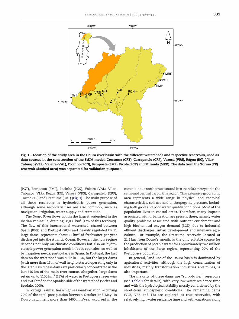
Fig. 1 – Location of the study area in the Douro river basin with the different watersheds and respective reservoirs, used as

data sources in the construction of the StDM model: Crestuma (CRT), Carrapatelo (CRP), Varosa (VRS), Ragua (RG), Vilar-

Tabuaco (VLR), Valeira (VAL), Pocinho (PCN), Bemposta (BMP), Picote (PCT) and Miranda (MRD). The data from the Torrao (TR)

reservoir (dashed area) was separated for validation purposes.

e c o l o g i c a l i n d i c a t o r s 9 ( 2 0 0 9 ) 3 2 9 – 3 4 5 331

(PCT), Bemposta (BMP), Pocinho (PCN), Valeira (VAL), Vilar-

Tabuaco (VLR), Regua (RG), Varosa (VRS), Carrapatelo (CRP),

Torrao (TR) and Crestuma (CRT) (Fig. 1). The main purpose of

all these reservoirs is hydroelectric power generation,

although some secondary uses are also common, such as

navigation, irrigation, water supply and recreation.

The Douro River flows within the largest watershed in the

Iberian Peninsula, draining 98,000 km2 (17% of this territory).

The flow of this international watershed, shared between

Spain (80%) and Portugal (20%) and heavily regulated by 51

large dams, represents about 15 km3 of freshwater per year

discharged into the Atlantic Ocean. However, the flow regime

depends not only on climatic conditions but also on hydro-

electric power generation needs in both countries, as well as

by irrigation needs, particularly in Spain. In Portugal, the first

dam on the watershed was built in 1920, but the larger dams

(with more than 15 m of wall height) started operating only in

the late 1950s. These dams are particularly concentrated in the

last 350 km of the main river course. Altogether, large dams

retain up to 1100 hm3 (13%) of water in Portuguese reservoirs

and 7500 hm3 on the Spanish side of the watershed (Vieira and

Bordalo, 2000).

In Portugal, rainfall has a high seasonal variation, occurring

70% of the total precipitation between October and May. In

Douro catchment more than 1400 mm/year occurred in the

mountainous northern areas and less than 500 mm/year in the

semi-arid central part of this region. This extensive geographic

area represents a wide range in physical and chemical

characteristics, soil use and anthropogenic pressure, includ-

ing both good and poor water quality conditions. Most of the

population lives in coastal areas. Therefore, many impacts

associated with urbanization are present there, namely water

quality problems associated with nutrient enrichment and

high biochemical oxygen demand (BOD) due to industrial

effluent discharges, urban development and intensive agri-

culture. For example, the Crestuma reservoir, located at

21.6 km from Douro’s mouth, is the only suitable source for

the production of potable water for approximately two million

inhabitants of the Porto region, representing 20% of the

Portuguese population.

In general, land use of the Douro basin is dominated by

agricultural activities, although the high concentration of

industries, mainly transformation industries and mines, is

also important.

The majority of these dams are ‘‘run-of-river’’ reservoirs

(see Table 1 for details), with very low water residence time

and with the hydrological stability mostly conditioned by the

short-term atmospheric conditions. The remaining dams

(VLR, VRS and TR) are explored as true reservoirs, with

relatively high water residence time and with variations along

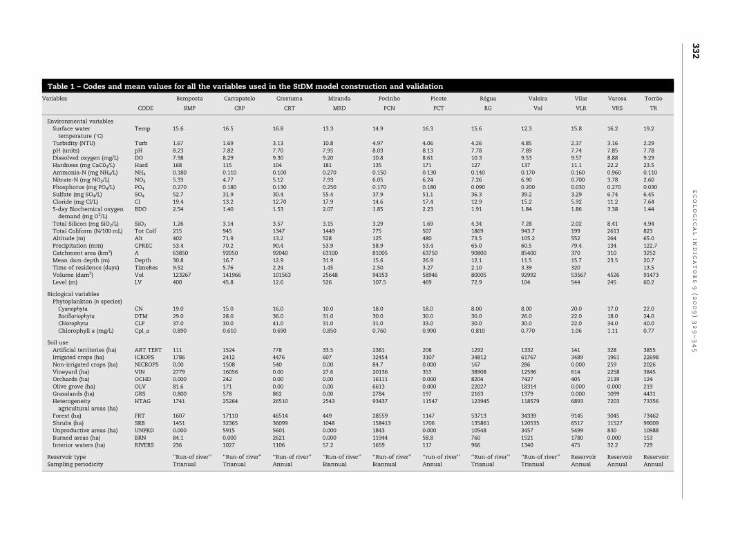
Table 1 – Codes and mean values for all the variables used in the StDM model construction and validation

Variables Bemposta Carrapatelo Crestuma Miranda Pocinho Picote Regua Valeira Vilar Varosa Torrao

CODE BMP CRP CRT MRD PCN PCT RG Val VLR VRS TR

Environmental variablesSurface water

temperature (8C)Temp 15.6 16.5 16.8 13.3 14.9 16.3 15.6 12.3 15.8 16.2 19.2

Turbidity (NTU) Turb 1.67 1.69 3.13 10.8 4.97 4.06 4.26 4.85 2.37 3.16 2.29pH (units) pH 8.23 7.82 7.70 7.95 8.03 8.13 7.78 7.89 7.74 7.85 7.78Dissolved oxygen (mg/L) DO 7.98 8.29 9.30 9.20 10.8 8.61 10.3 9.53 9.57 8.88 9.29Hardness (mg CaC03/L) Hard 168 115 104 181 135 171 127 137 11.1 22.2 23.5Ammonia-N (mg NH4/L) NH4 0.180 0.110 0.100 0.270 0.150 0.130 0.140 0.170 0.160 0.960 0.110Nitrate-N (mg NO3/L) NO3 5.33 4.77 5.12 7.93 6.05 6.24 7.26 6.90 0.700 3.78 2.60Phosphorus (mg PO4/L) PO4 0.270 0.180 0.130 0.250 0.170 0.180 0.090 0.200 0.030 0.270 0.030Sulfate (mg SO4/L) SO4 52.7 31.9 30.4 55.4 37.9 51.1 36.3 39.2 3.29 6.74 6.45Cloride (mg Cl/L) Cl 19.4 13.2 12.70 17.9 14.6 17.4 12.9 15.2 5.92 11.2 7.645-day Biochemical oxygen

demand (mg O2/L)BDO 2.54 1.40 1.53 2.07 1.85 2.23 1.91 1.84 1.86 3.38 1.44

Total Silicon (mg SiO2/L) SiO2 1.26 3.14 3.57 3.15 3.29 1.69 4.34 7.28 2.02 8.41 4.94Total Coliform (N/100 mL) Tot Colf 215 945 1347 1449 775 507 1869 943.7 199 2613 823Altitude (m) Alt 402 71.9 13.2 528 125 480 73.5 105.2 552 264 65.0Precipitation (mm) CPREC 53.4 70.2 90.4 53.9 58.9 53.4 65.0 60.5 79.4 134 122.7Catchment area (km2) A 63850 92050 92040 63100 81005 63750 90800 85400 370 310 3252Mean dam depth (m) Depth 30.8 16.7 12.9 31.9 15.6 26.9 12.1 11.5 15.7 23.5 20.7Time of residence (days) TimeRes 9.52 5.76 2.24 1.45 2.50 3.27 2.10 3.39 320 13.5Volume (dam3) Vol 123267 141966 101563 25648 94353 58946 80005 92992 53567 4526 91473Level (m) LV 400 45.8 12.6 526 107.5 469 72.9 104 544 245 60.2

Biological variablesPhytoplankton (n species)

Cyanophyta CN 19.0 15.0 16.0 10.0 18.0 18.0 8.00 8.00 20.0 17.0 22.0Bacillariophyta DTM 29.0 28.0 36.0 31.0 30.0 30.0 30.0 26.0 22.0 18.0 24.0Chlorophyta CLP 37.0 30.0 41.0 31.0 31.0 33.0 30.0 30.0 22.0 34.0 40.0Chlorophyll a (mg/L) Cpl_a 0.890 0.610 0.690 0.850 0.760 0.990 0.810 0.770 1.06 1.11 0.77

Soil useArtificial territories (ha) ART TERT 111 1524 778 33.5 2381 208 1292 1332 141 328 3855Irrigated crops (ha) ICROPS 1786 2412 4476 607 32454 3107 34812 61767 3489 1961 22698Non-irrigated crops (ha) NICROPS 0.00 1508 540 0.00 84.7 0.000 167 286 0.000 259 2026Vineyard (ha) VIN 2779 16056 0.00 27.6 20136 353 38908 12596 614 2258 3845Orchards (ha) OCHD 0.000 242 0.00 0.00 16111 0.000 8204 7427 405 2139 124Olive grove (ha) OLV 81.6 171 0.00 0.00 6613 0.000 22027 18314 0.000 0.000 219Grasslands (ha) GRS 0.800 578 862 0.00 2784 197 2163 1379 0.000 1099 4431Heterogeneity

agricultural areas (ha)HTAG 1741 25264 26510 2543 93437 11547 123945 118579 6893 7203 73356

Forest (ha) FRT 1607 17110 46514 449 28559 1147 53713 34339 9145 3045 73462Shrubs (ha) SRB 1451 32365 36099 1048 158413 1706 135861 120535 6517 11527 99009Unproductive areas (ha) UNPRD 0.000 5915 5601 0.000 1843 0.000 10548 3457 5499 830 10988Burned areas (ha) BRN 84.1 0.000 2621 0.000 11944 58.8 760 1521 1780 0.000 153Interior waters (ha) RIVERS 236 1027 1106 57.2 1659 117 966 1340 475 32.2 729

Reservoir type ‘‘Run-of river’’ ‘‘Run-of river’’ ‘‘Run-of river’’ ‘‘Run-of river’’ ‘‘Run-of river’’ ‘‘run-of river’’ ‘‘Run-of river’’ ‘‘Run-of river’’ Reservoir Reservoir ReservoirSampling periodicity Trianual Trianual Annual Biannual Biannual Annual Trianual Trianual Annual Annual Annual

ec

ol

og

ic

al

in

dic

at

or

s9

(2

00

9)

32

9–

34

53

32

e c o l o g i c a l i n d i c a t o r s 9 ( 2 0 0 9 ) 3 2 9 – 3 4 5 333

the year mostly related to the seasonality of the inputs of

water. The main characteristics of the studied reservoirs are

presented in Table 1.

2.2. Environmental variables and chlorophyll a

The environmental and biological variables were measured by

the national Laboratory of Environment and Applied Chem-

istry (LABLEC), from 1996 to 2004, four times per year,

corresponding to spring, summer, autumn and winter. These

variables were sampled according to the methodologies

described by CEN/TC 230. All samples were collected at

100 m from the reservoirs’s crest, at approximately 0.5 m

depth. From all reservoirs, 58.8% were sampled annually,

26.5% biannually and 14.7% triennially (Table 1).

To determined soil use dynamics in Douro watershed, i.e.,

rates of soil use alterations, a geographic information system

database was created (ESRI, ArcGIS 9.0), with 13 spatial

variables (see Table 1). These use/land cover variables derived

primarily from the Corine Land Cover from two distinct

decades 1990 and 2000 (CLC, 1990 and 2000; IGEOE, 2006),

additionally the proportions of the predominant CLC classes in

the basin (urban areas, intensive and extensive agriculture,

natural and semi-natural areas and burned areas) were

calculated.

The trophic classification of reservoirs was obtained from

the OCDE model (Vollenweider and Kerekes, 1982), based on

Total Phosphorus, Shecchi Depth and Mean Chlorophyll a

concentration (see Table 1).

2.3. Biological variables

The phytoplankton samples were collected from 1996 to

2004, with the periodicity described for the environmental

parameters, using a Van Dorn bottle net, at a depth of

approximately 0.5 m. Phytoplankton community composi-

tion was studied through inverted microscopy, following

Utermohl’s method (Lund et al., 1958). For the quantification

and identification of phytoplankton, samples were fixed

in Lugol’s solution (1%, v/v) and, when possible, identified

to the species level. The abundance of each taxon

was estimated using a 5-score scale criteria (0-absent to

4-bloom).

2.4. Statistical analysis and modelling procedures

The soil use dataset, the base of the dynamic sub-model of our

StDM application (level 1), incorporates real gradients relying

on land cover alterations through one decade, from 1990s to

2000s, in the Douro river watershed.

A stepwise multiple-regression analysis (Zar, 1996) was

used to test relationships between the soil use dynamics

within the watershed (level 1) and the physicochemical

variables of the reservoir (level 2) and between these aquatic

environmental variables and the phytoplankton metrics (level

3). In level 2, the dependent variables, selected as representa-

tive of the physicochemical status of water column reservoir,

were: total coliforms, PO4, Cl, NH4, BOD5, pH, SiO2, DO, NO3,

hardness, turbidity and SO4. For this level, the independent

variables considered were the 13 soil use variables and the 5

stochastic environmental variables, namely surface water

temperature, precipitation, volume, level and water residence

time (see Table 1 for details).

In level 3, the dependent variables, selected as representa-

tive of the local phytoplankton, were: Cyanophyta (Blue-green

algae), Clorophyta (Green algae), Bacillariophyta (diatoms) and

Chlorophyll a. The independent variables considered for the

phytoplankton metrics were the 17 environmental variables

referred above for level 2 and for the stochastic environmental

variables.

From a bottom up perspective, each living component

interacts with other living components and non-living

features of their shared habitat. A step down procedure was

used to test the effect of each variable in the presence of all

other pertinent variables, with the least significant variable

being removed at every step. The analysis stopped when all

the remaining variables had a significant level P < 0.05 (Zar,

1996). The multi-level approach gives realism to the interac-

tions considered by incorporating into the model a typical

‘‘cascade effect’’ observed in these processes (Brazner et al.,

2007; Bailey et al., 2007). Therefore, in order to simplify the

model structure, only the main key-components were

introduced as representative ecological indicators, but which

obviously could be complemented by other relevant state

variables or other dynamic variables in further applications.

The specifications of all variables considered are indicated in

Table 1. Although the lack of normality distribution of the

dependent variables was not solved by any transformation

(Kolmogorov–Smirnov test), the linearity and the homosce-

dasticity of the residuals were achieved by using logarithmic

transformations (X0 = log[X + 1]) in each side of the equation,

i.e., on both the dependent and independent variables (Zar,

1996; Podani, 2000). The lack of substantial intercorrelation

among independent variables was confirmed by the inspec-

tion of the respective tolerance values. All the statistical

analysis was carried out using the software SYSTAT 8.01.

Since this statistical procedure was based on a very

complete database, covering true gradients of environmental

and biological characteristics of the reservoirs in the Douro

basin (Fig. 1), over space and time, the significant partial

regression coefficients were assumed as relevant holistic

ecological parameters in the dynamic model construction.

This is the heart of the philosophy of the StDM. In a holistic

perspective, the partial regression coefficients represent the

global influence of the environmental variables selected,

which are of significant importance on several complex

ecological processes. To develop the dynamic model the

software STELLA 8.1.41 was used.

Water quality indices and trophic level classification

system are useful tools for enhancing communications

between scientists, water managers, policymakers and/or

the general public. Therefore, some of the ecological indicators

selected were described using Carlson’s Trophic Status Index

(TSI). The status for Secchi depth (SD), chlorophyll a (Clp a) and

total phosphorus (TP) were described using the following

equations (Carlson, 1977):

TSIðSDÞ ¼ 60� 14:41� ln SDðmÞ;TSIðClp aÞ ¼ 9:81� ln Clp aðmg=LÞ þ 30:6;TSIðTPÞ ¼ 14:42� ln TPðmg=LÞ þ 4:15:

e c o l o g i c a l i n d i c a t o r s 9 ( 2 0 0 9 ) 3 2 9 – 3 4 5334

Other indices have been constructed to be used as a

complement of these basic three. Since nitrogen limitation

still classifies a lake along Naumann’s nutrient axis, the effect

of nitrogen limitation can be estimated by having a companion

index to the TSI(TP). Therefore, the TSI(TN) was introduced in

the model and calculated using the following formula (Kratzer

et al., 1982):

TSIðTNÞ ¼ 54:45þ 14:43� ln TNðmg=LÞ:

A major strength of TSI is that the interrelationships

between variables can be used to identify certain conditions in

the lake or reservoir that are related to the factors that limit

algal biomass or affect the measured variables. The concept of

trophic status is based on the fact that changes in nutrient

levels (measured by TP and NT) causes changes in algal

biomass (estimated by Clp_a measures) which in turn causes

changes in lake clarity (measured by SD). TSI values greater

than 50 are associated with eutrophy (high productivity). The

range between 40 and 50 is usually associated with meso-

trophy (moderate productivity) and values less than 40 are

associated with oligotrophy (low productivity) (Carlson, 1981,

1983). Since some of these trophic variables do not survive

when the initial stepwise multi-regression analysis was

carried out, namely TP and SD, significant relationships were

found between them and other environmental variables from

the StDM model. Therefore, simple linear regression models

were introduced in the model in way to estimate the

concentration of total phosphorus from total nitrogen con-

centration (TN, as a sum of NO3 and NH4) (y = 0.018x + 0.023;

R2 = 0.348; N = 25) and Secchi disk transparency from turbidity

(y = 0.775x + 3.83; R2 = 0.732; N = 25).

For validation purposes, a set of biological and environ-

mental data (including land cover) from the Torrao reservoir,

that are independent of the data used to structure the StDM

model and estimate its parameters, were used to confront the

simulated values of a given state variable with the real values

of the same component. A regression analysis (MODEL II) was

performed to compare the observed real values of the selected

variables with the expected values obtained by model

simulations for the same periods. At the end of each analysis,

the 95% confidence limits for the intercept and the slope of the

regression line were determined which, together with the

results of the respective analysis of variance (ANOVA), allowed

to assess the proximity of the simulations produced with the

observed values (Sokal and Rohlf, 1995). When the results of

the regression analysis were statistically significant, i.e., when

the intercept of the regression line was not statistically

different from 0 and the slope was not statistically different

from 1, the model simulations were considered validated

(Sokal and Rohlf, 1995; Oberdorf et al., 2001).

The model is prepared to work with table functions for

validation purposes (Validation Mode) and to produce sto-

chastic simulations based on the monthly stochastic varia-

bility of some environmental variables (Random Mode).

Simulations based on stochastic principles take into con-

sideration the random behaviour of some environmental

variables with influence on the studied ecological phenomena.

The limit values of environmental variables were determined,

from the period between December 1995 and December 2004,

to discriminate the maximum and minimum values of each

stochastic environmental variable, included in the model as a

RANDOM function (Annex 1, Other functions). The selection of

the model working mode is done by switching the toggle

option between 0 and 1 for validation or stochastic calcula-

tions, respectively. The Annex 1 is available in the online

version of this article as Electronic Supplementary Material.

3. Results and discussion

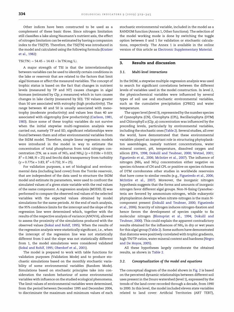
3.1. Multi-level interactions

In the StDM, a stepwise multiple-regression analysis was used

to search for significant correlations between the different

levels of variables used in the model construction. In level 2,

the physicochemical variables were influenced by several

types of soil use and stochastic environmental variables,

such as the cumulative precipitation (CPREC) and water

temperature.

The upper level (level 3), represented by the number species

of Cyanophyta (CN), Clorophyta (CPL), Bacillariophyta (DTM)

and Chlorophyll a (Clp_a) concentration was influenced by the

preceding levels, particularly by environmental variables,

including the stochastic ones (Table 2). Several studies, all over

the world, have demonstrated that these environmental

variables played an important role in structuring phytoplank-

ton assemblages, namely nutrient concentrations, water

mineral content, pH, temperature, dissolved oxygen and

silicon (EPA, 1998; Dokulil and Teubner, 2000; Wetzel, 2001;

Figueiredo et al., 2006; McIntire et al., 2007). The influence of

nitrogen (NH4 and NO3) concentration either negative on

species richness of CN and CPL or positive on species richness

of DTM corroborates other studies in worldwide reservoirs

that have come to similar results (e.g., Figueiredo et al., 2006;

McIntire et al., 2007). Moreover, the inorganic nitrogen

hypothesis suggests that the forms and amounts of inorganic

nitrogen favor different algal groups. Non-N-fixing Cyanobac-

teria are favored by ammonium-nitrogen, while eukaryotic

phytoplankton develops when nitrate-nitrogen is the main N-

component present (Dokulil and Teubner, 2000; Figueiredo

et al., 2006). Scarcity of nitrogen induces nitrogen-fixation and

hence favors the development of species capable to fix

molecular nitrogen (Blomqvist et al., 1994; Dokulil and

Teubner, 2000). This could explain the apparent contradictory

results obtained for the influences of NH4 in dry or wet years

for this algal group (Table 2). Some authors have demonstrated

that diatoms were positively correlated with trophic gradients,

high TN/TP-ratios, water mineral content and hardness (Negro

and De Hoyos, 2005).

All these hypotheses largely corroborate the obtained

results, as shown in Table 2.

3.2. Conceptualization of the model and equations

The conceptual diagram of the model shown in Fig. 2 is based

on the perceived dynamic relationships between different soil

uses present in the Douro watershed (level 1), expressed by the

trends of the land cover recorded through a decade, from 1990

to 2000. In this level, the model included eleven state variables

related to land cover: Artificial Territories (ART TERT),

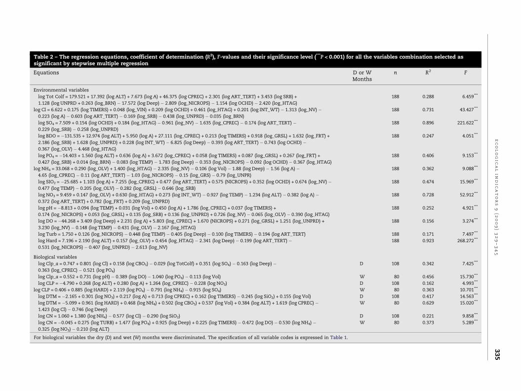
Table 2 – The regression equations, coefficient of determination (R2), F-values and their significance level (***P < 0.001) for all the variables combination selected assignificant by stepwise multiple regression

Equations D or WMonths

n R2 F

Environmental variables

log Tot Colf = 179.521 + 17.392 (log ALT) + 7.673 (log A) + 46.375 (log CPREC) + 2.301 (log ART_TERT) + 3.453 (log SRB) +

1.128 (log UNPRD + 0.263 (log_BRN) � 17.572 (log Deep) � 2.809 (log_NICROPS) � 1.154 (log OCHD) � 2.420 (log_HTAG)

188 0.288 6.459***

log Cl = 6.622 + 0.175 (log TIMERS) + 0.048 (log_VIN) + 0.209 (log OCHD) + 0.461 (log_HTAG) + 0.201 (log INT_WT) � 1.313 (log_NV) �0.223 (log A) � 0.603 (log ART_TERT) � 0.169 (log_SRB) � 0.438 (log_UNPRD) � 0.035 (log_BRN)

188 0.731 43.427***

log SO4 = 7.509 + 0.154 (log OCHD) + 0.184 (log_HTAG) � 0.961 (log_NV) � 1.635 (log_CPREC) � 0.174 (log ART_TERT) �0.229 (log_SRB) � 0.258 (log_UNPRD)

188 0.896 221.622***

log BDO = �131.535 + 12.974 (log ALT) + 5.950 (log A) + 27.111 (log_CPREC) + 0.213 (log TIMERS) + 0.918 (log_GRSL) + 1.632 (log_FRT) +

2.186 (log_SRB) + 1.628 (log_UNPRD) + 0.228 (log INT_WT) � 6.825 (log Deep) � 0.393 (log ART_TERT) � 0.743 (log OCHD) �0.367 (log_OLV) � 4.468 (log_HTAG)

188 0.247 4.051***

log PO4 = �14.403 + 1.560 (log ALT) + 0.636 (log A) + 3.672 (log_CPREC) + 0.058 (log TIMERS) + 0.087 (log_GRSL) + 0.267 (log_FRT) +

0.427 (log_SRB) + 0.014 (log_BRN) � 0.083 (log TEMP) � 1.783 (log Deep) � 0.353 (log_NICROPS) � 0.092 (log OCHD) � 0.367 (log_HTAG)

188 0.406 9.153***

log NH4 = 33.068 + 0.290 (log_OLV) + 1.400 (log_HTAG) � 2.335 (log_NV) � 0.106 (log Vol) � 1.88 (log Deep) � 1.56 (log A) �4.65 (log_CPREC) � 0.11 (log ART_TERT) � 1.03 (log_NICROPS) � 0.15 (log_GRS) � 0.79 (log_UNPR)

188 0.362 9.088***

log SIO2 = �25.685 + 1.103 (log A) + 7.255 (log_CPREC) + 0.477 (log ART_TERT) + 0.575 (NICROPS) + 0.352 (log OCHD) + 0.674 (log_NV) �0.477 (log TEMP) � 0.205 (log_OLV) � 0.282 (log_GRSL) � 0.646 (log_SRB)

188 0.474 15.969***

log NO3 = 9.459 + 0.147 (log_OLV) + 0.630 (log_HTAG) + 0.273 (log INT_WT) � 0.927 (log TEMP) � 1.234 (log ALT) � 0.382 (log A) �0.372 (log ART_TERT) + 0.782 (log_FRT) + 0.209 (log_UNPRD)

188 0.728 52.912***

log pH = �8.813 + 0.094 (log TEMP) + 0.031 (log Vol) + 0.450 (log A) + 1.786 (log_CPREC) + 0.037 (log TIMERS) +

0.174 (log_NICROPS) + 0.053 (log_GRSL) + 0.135 (log_SRB) + 0.136 (log_UNPRD) + 0.726 (log_NV) � 0.065 (log_OLV) � 0.390 (log_HTAG)

188 0.252 4.921***

log DO = �44.268 + 3.409 (log Deep) + 2.231 (log A) + 5.803 (log_CPREC) + 1.670 (NICROPS) + 0.271 (log_GRSL) + 1.251 (log_UNPRD) +

3.230 (log_NV) � 0.148 (log TEMP) � 0.431 (log_OLV) � 2.167 (log_HTAG)

188 0.156 3.274***

log Turb = 1.750 + 0.126 (log_NICROPS) � 0.448 (log TEMP) � 0.405 (log Deep) � 0.100 (log TIMERS) � 0.194 (log ART_TERT) 188 0.171 7.497***

log Hard = 7.196 + 2.190 (log ALT) + 0.157 (log_OLV) + 0.454 (log_HTAG) � 2.341 (log Deep) � 0.199 (log ART_TERT) �0.531 (log_NICROPS) � 0.407 (log_UNPRD) � 2.613 (log_NV)

188 0.923 268.272***

Biological variables

log Clp_a = 0.747 + 0.801 (log Cl) + 0.158 (log CBO5) � 0.029 (log TotColf) + 0.351 (log SO4) � 0.163 (log Deep) �0.363 (log_CPREC) � 0.521 (log PO4)

D 108 0.342 7.425***

log Clp_a = 0.552 + 0.731 (log pH) � 0.389 (log DO) � 1.040 (log PO4) � 0.113 (log Vol) W 80 0.456 15.730***

log CLP = �4.790 + 0.268 (log ALT) + 0.280 (log A) + 1.264 (log_CPREC) � 0.228 (log NO3) D 108 0.162 4.993***

log CLP = 0.406 + 0.885 (log HARD) + 2.119 (log PO4) � 0.791 (log NH4) � 0.915 (log SO4) W 80 0.363 10.701***

log DTM = �2.165 + 0.301 (log NO3) + 0.217 (log A) + 0.713 (log CPREC) + 0.162 (log TIMERS) � 0.245 (log SiO2) + 0.155 (log Vol) D 108 0.417 14.563***

log DTM = �5.099 + 0.961 (log HARD) + 0.468 (log NH4) + 0.502 (log CBO5) + 0.537 (log Vol) + 0.384 (log ALT) + 1.619 (log CPREC) �1.423 (log Cl) � 0.746 (log Deep)

W 80 0.629 15.020***

log CN = 1.060 + 1.380 (log NH4) � 0.577 (log Cl) � 0.290 (log SiO2) D 108 0.221 9.858***

log CN = �0.045 + 0.275 (log TURB) + 1.477 (log PO4) + 0.925 (log Deep) + 0.225 (log TIMERS) � 0.472 (log DO) � 0.530 (log NH4) �0.325 (log NO3) � 0.210 (log ALT)

W 80 0.373 5.289***

For biological variables the dry (D) and wet (W) months were discriminated. The specification of all variable codes is expressed in Table 1.

ec

ol

og

ic

al

in

dic

at

or

s9

(2

00

9)

32

9–

34

53

35

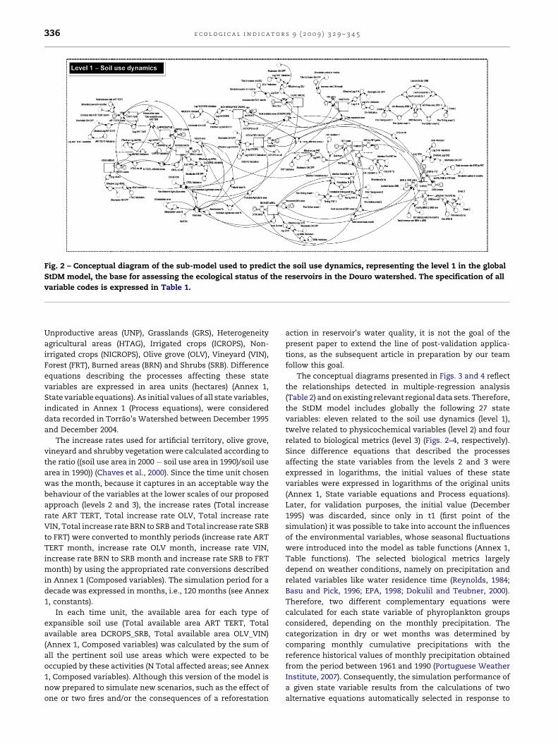
Fig. 2 – Conceptual diagram of the sub-model used to predict the soil use dynamics, representing the level 1 in the global

StDM model, the base for assessing the ecological status of the reservoirs in the Douro watershed. The specification of all

variable codes is expressed in Table 1.

e c o l o g i c a l i n d i c a t o r s 9 ( 2 0 0 9 ) 3 2 9 – 3 4 5336

Unproductive areas (UNP), Grasslands (GRS), Heterogeneity

agricultural areas (HTAG), Irrigated crops (ICROPS), Non-

irrigated crops (NICROPS), Olive grove (OLV), Vineyard (VIN),

Forest (FRT), Burned areas (BRN) and Shrubs (SRB). Difference

equations describing the processes affecting these state

variables are expressed in area units (hectares) (Annex 1,

State variable equations). As initial values of all state variables,

indicated in Annex 1 (Process equations), were considered

data recorded in Torrao’s Watershed between December 1995

and December 2004.

The increase rates used for artificial territory, olive grove,

vineyard and shrubby vegetation were calculated according to

the ratio ((soil use area in 2000 � soil use area in 1990)/soil use

area in 1990)) (Chaves et al., 2000). Since the time unit chosen

was the month, because it captures in an acceptable way the

behaviour of the variables at the lower scales of our proposed

approach (levels 2 and 3), the increase rates (Total increase

rate ART TERT, Total increase rate OLV, Total increase rate

VIN, Total increase rate BRN to SRB and Total increase rate SRB

to FRT) were converted to monthly periods (increase rate ART

TERT month, increase rate OLV month, increase rate VIN,

increase rate BRN to SRB month and increase rate SRB to FRT

month) by using the appropriated rate conversions described

in Annex 1 (Composed variables). The simulation period for a

decade was expressed in months, i.e., 120 months (see Annex

1, constants).

In each time unit, the available area for each type of

expansible soil use (Total available area ART TERT, Total

available area DCROPS_SRB, Total available area OLV_VIN)

(Annex 1, Composed variables) was calculated by the sum of

all the pertinent soil use areas which were expected to be

occupied by these activities (N Total affected areas; see Annex

1, Composed variables). Although this version of the model is

now prepared to simulate new scenarios, such as the effect of

one or two fires and/or the consequences of a reforestation

action in reservoir’s water quality, it is not the goal of the

present paper to extend the line of post-validation applica-

tions, as the subsequent article in preparation by our team

follow this goal.

The conceptual diagrams presented in Figs. 3 and 4 reflect

the relationships detected in multiple-regression analysis

(Table 2) and on existing relevant regional data sets. Therefore,

the StDM model includes globally the following 27 state

variables: eleven related to the soil use dynamics (level 1),

twelve related to physicochemical variables (level 2) and four

related to biological metrics (level 3) (Figs. 2–4, respectively).

Since difference equations that described the processes

affecting the state variables from the levels 2 and 3 were

expressed in logarithms, the initial values of these state

variables were expressed in logarithms of the original units

(Annex 1, State variable equations and Process equations).

Later, for validation purposes, the initial value (December

1995) was discarded, since only in t1 (first point of the

simulation) it was possible to take into account the influences

of the environmental variables, whose seasonal fluctuations

were introduced into the model as table functions (Annex 1,

Table functions). The selected biological metrics largely

depend on weather conditions, namely on precipitation and

related variables like water residence time (Reynolds, 1984;

Basu and Pick, 1996; EPA, 1998; Dokulil and Teubner, 2000).

Therefore, two different complementary equations were

calculated for each state variable of phyroplankton groups

considered, depending on the monthly precipitation. The

categorization in dry or wet months was determined by

comparing monthly cumulative precipitations with the

reference historical values of monthly precipitation obtained

from the period between 1961 and 1990 (Portuguese Weather

Institute, 2007). Consequently, the simulation performance of

a given state variable results from the calculations of two

alternative equations automatically selected in response to

Fig. 3 – Conceptual diagram of the sub-model used to predict the responses of the water column environmental variables to

changes due to soil use dynamics, representing the level 2 in the StDM model for the Douro watershed reservoirs. The

specification of all variable codes is expressed in Table 1.

e c o l o g i c a l i n d i c a t o r s 9 ( 2 0 0 9 ) 3 2 9 – 3 4 5 337

the monthly precipitation influence (Fig. 4, Table 2 and Annex

1, State variable equations). The inflows affecting the state

variables, in levels 2 and 3, were based on the positive

constants and all positive partial coefficients of each variable

resulting from the previous multiple-regression analysis

(Figs. 3 and 4, Table 2 and Annex 1, State variable and Process

equations). Chlorophyll a and the number of species of

Cyanophyta, Bacillariophyta and Chlorophyta were affected by

two inflows corresponding to the conditions of dry or wet

months (Clp_a gains Dry, Clp_a gains Wet, CLP gains Dry, CLP

gains Wet, CN gains Dry, CN gains Wet, DTM gains Dry and

DTM gains Wet). Using the same criteria, each one of these

state variables was affected by two outflows related to the

negative constants and partial regression coefficients (Figs. 3

and 4, Table 2 and Annex 1, State variable and Process

equations) (Clp_a losses Dry, Clp_a losses Wet, CLP losses Dry,

CLP losses Wet, CN losses Dry, CN losses Wet, DTM losses Dry,

DTM losses Wet). To complement the information about the

ecological status of reservoir’s water quality, the trophic state

indices (TSI) based on chlorophyll a, total nitrogen, total

phosphorus and Secchi disk depth outputs were introduced

into the model (Figs. 3 and 4, Annex 1, Composed variables).

Although the StDM simulations for each physicochemical or

biological metric were composed of a given value per time

unit, the respective state variable might had a cumulative

behaviour over time in response to environmental condition

changes. Therefore, to prevent this from happening, sixteen

outflow adjustments were incorporated in the model (Level 2:

BDO adjust, Cl adjust, Hard adjust, NH4 adjust, NO3 adjust, DO

adjust, pH adjust, PO4 adjust, SiO2 adjust, SO4 adjust, TotColf

adjust, Turb adjust; Level 3: Clp_a adjust, CLP adjust, CN

adjust, and DTM adjust) aiming to empty the state variables at

each time step, by a ‘‘flushing cistern mechanism’’, before

beginning the next step with new environmental influences

(Figs. 2 and 3, Annex 1, State variable and Process equations).

For process compatibilities and a more realistic comprehen-

sion of the model simulations, some conversions were

introduced, denominated associated variables (Figs. 2–4 and

Annex 1, Associated variables). Regarding biological and

physicochemical variables, these conversions were obtained

through an inverse transformation (anti-logarithmic), which

transforms logarithms into the original measurement units

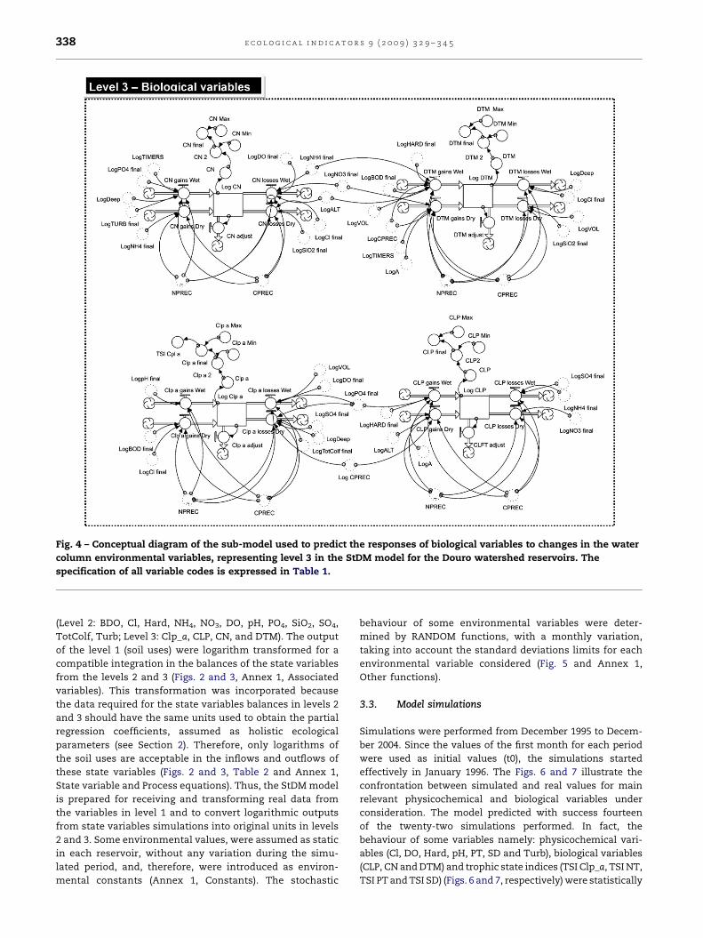
Fig. 4 – Conceptual diagram of the sub-model used to predict the responses of biological variables to changes in the water

column environmental variables, representing level 3 in the StDM model for the Douro watershed reservoirs. The

specification of all variable codes is expressed in Table 1.

e c o l o g i c a l i n d i c a t o r s 9 ( 2 0 0 9 ) 3 2 9 – 3 4 5338

(Level 2: BDO, Cl, Hard, NH4, NO3, DO, pH, PO4, SiO2, SO4,

TotColf, Turb; Level 3: Clp_a, CLP, CN, and DTM). The output

of the level 1 (soil uses) were logarithm transformed for a

compatible integration in the balances of the state variables

from the levels 2 and 3 (Figs. 2 and 3, Annex 1, Associated

variables). This transformation was incorporated because

the data required for the state variables balances in levels 2

and 3 should have the same units used to obtain the partial

regression coefficients, assumed as holistic ecological

parameters (see Section 2). Therefore, only logarithms of

the soil uses are acceptable in the inflows and outflows of

these state variables (Figs. 2 and 3, Table 2 and Annex 1,

State variable and Process equations). Thus, the StDM model

is prepared for receiving and transforming real data from

the variables in level 1 and to convert logarithmic outputs

from state variables simulations into original units in levels

2 and 3. Some environmental values, were assumed as static

in each reservoir, without any variation during the simu-

lated period, and, therefore, were introduced as environ-

mental constants (Annex 1, Constants). The stochastic

behaviour of some environmental variables were deter-

mined by RANDOM functions, with a monthly variation,

taking into account the standard deviations limits for each

environmental variable considered (Fig. 5 and Annex 1,

Other functions).

3.3. Model simulations

Simulations were performed from December 1995 to Decem-

ber 2004. Since the values of the first month for each period

were used as initial values (t0), the simulations started

effectively in January 1996. The Figs. 6 and 7 illustrate the

confrontation between simulated and real values for main

relevant physicochemical and biological variables under

consideration. The model predicted with success fourteen

of the twenty-two simulations performed. In fact, the

behaviour of some variables namely: physicochemical vari-

ables (Cl, DO, Hard, pH, PT, SD and Turb), biological variables

(CLP, CN and DTM) and trophic state indices (TSI Clp_a, TSI NT,

TSI PT and TSI SD) (Figs. 6 and 7, respectively) were statistically

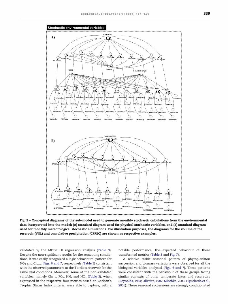
Fig. 5 – Conceptual diagrams of the sub-model used to generate monthly stochastic calculations from the environmental

data incorporated into the model: (A) standard diagram used for physical stochastic variables, and (B) standard diagram

used for monthly meteorological stochastic simulations. For illustration purposes, the diagrams for the volume of the

reservoir (VOL) and cumulative precipitation (CPREC) are shown as respective examples.

e c o l o g i c a l i n d i c a t o r s 9 ( 2 0 0 9 ) 3 2 9 – 3 4 5 339

validated by the MODEL II regression analysis (Table 3).

Despite the non-significant results for the remaining simula-

tions, it was easily recognized a logic behavioural pattern for

NO3 and Clp_a (Figs. 6 and 7, respectively; Table 3) consistent

with the observed parameters at the Torrao’s reservoir for the

same real conditions. Moreover, some of the non-validated

variables, namely Clp_a, PO4, NH4 and NO3 (Table 3), when

expressed in the respective four metrics based on Carlson’s

Trophic Status Index criteria, were able to capture, with a

notable performance, the expected behaviour of these

transformed metrics (Table 3 and Fig. 7).

A relative stable seasonal pattern of phytoplankton

succession and biomass variations were observed for all the

biological variables analysed (Figs. 6 and 7). These patterns

were consistent with the behaviour of these groups facing

similar contexts of other temperate lakes and reservoirs

(Reynolds, 1984; Oliveira, 1987; Mischke, 2003; Figueiredo et al.,

2006). These seasonal successions are strongly conditionated

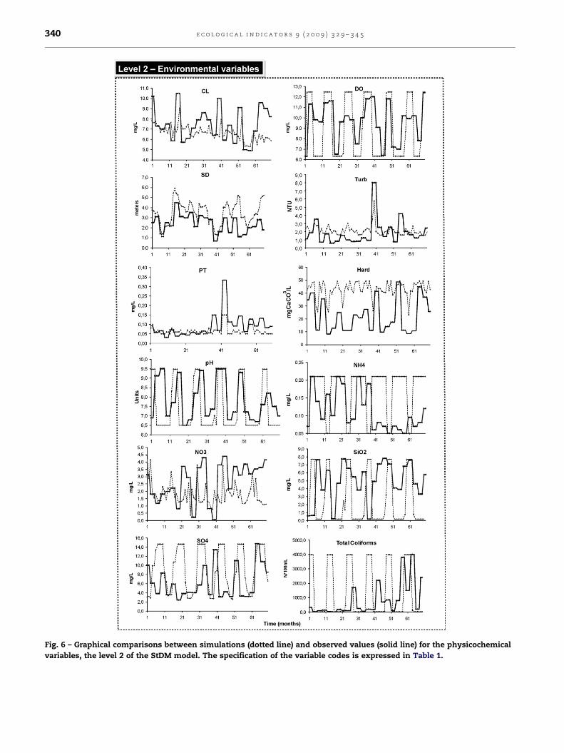
Fig. 6 – Graphical comparisons between simulations (dotted line) and observed values (solid line) for the physicochemical

variables, the level 2 of the StDM model. The specification of the variable codes is expressed in Table 1.

e c o l o g i c a l i n d i c a t o r s 9 ( 2 0 0 9 ) 3 2 9 – 3 4 5340

Fig. 7 – Graphical comparisons between simulations (dotted line) and observed values (solid line) for the biological variables

and for the trophic status indices analysed, the level 3 of the StDM model. The specification of the variable codes is

expressed in Table 1.

e c o l o g i c a l i n d i c a t o r s 9 ( 2 0 0 9 ) 3 2 9 – 3 4 5 341

by meteorological and stratification-mixing processes (Wet-

zel, 2001). Therefore, the variation in the abundance of the

total phytoplankton, represented by the chlorophyll a content

simulations, shown a credible seasonal pattern with an earlier

maximum occurring through spring and early summer to a

maximum in July, and a second peak associated with early

stages of autumnal destratification. This ‘‘dimictic’’ pattern is

probably typical of many ‘‘mesotrophic’’ shallow (<30 m)

temperate lakes and reservoirs (Reynolds, 1984; Wetzel, 2001;

Mischke, 2003). It is supposed that the two peaks reflect the

coincidence of physically suitable growth conditions, with

relatively high concentrations of limiting nutrients shortages

of which prevent the attainment of large biomasses during the

midsummer period (Reynolds, 1984; Domingues and Galvao,

2007). Seasonal succession pattern of phytoplankton in

temperate dimictic reservoirs, similar to Torrao, usually

involves a winter minimum with species adapted to low light

and temperature, a late winter-spring and autumn peaks of

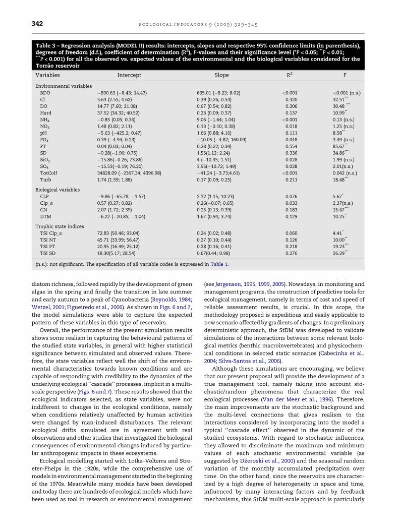
Table 3 – Regression analysis (MODEL II) results: intercepts, slopes and respective 95% confidence limits (in parenthesis),degrees of freedom (d.f.), coefficient of determination (R2), F-values and their significance level (*P < 0.05; **P < 0.01;***P < 0.001) for all the observed vs. expected values of the environmental and the biological variables considered for theTorrao reservoir

Variables Intercept Slope R2 F

Environmental variables

BDO �890.63 (�8.43; 14.43) 635.01 (�8.23; 8.02) <0.001 <0.001 (n.s.)

Cl 3.63 (2.55; 4.62) 0.39 (0.26; 0.54) 0.320 32.51***

DO 14.77 (7.60; 21.08) 0.67 (0.54; 0.82) 0.306 30.48 ***

Hard 37.52 (34.32; 40.52) 0.23 (0.09; 0.37) 0.137 10.99**

NH4 �0.85 (0.05; 0.34) 9.06 (�1.64; 1.04) <0.001 0.13 (n.s.)

NO3 1.48 (0.82; 2.11) 0.13 (�0.10; 0.38) 0.018 1.25 (n.s.)

pH �5.63 (�425.2; 0.47) 1.66 (0.88; 4.16) 0.111 8.58**

PO4 0.39 (�4.94; 0.23) �10.05 (�4.82; 160.09) 0.048 3.49 (n.s.)

PT 0.04 (0.03; 0.04) 0.28 (0.22; 0.34) 0.554 85.67***

SD �0.28(�1.96; 0.75) 1.55(1.12; 2.24) 0.336 34.86***

SiO2 �15.86(�0.26; 73.86) 4 (�10.35; 1.51) 0.028 1.99 (n.s.)

SO4 �15.53(�0.19; 76.20) 3.95(�10.72; 1.49) 0.028 2.01(n.s.)

TotColf 34828.09 (�2367.34; 4396.98) �41.24 (�3.73;4.61) <0.001 0.042 (n.s.)

Turb 1.74 (1.59; 1.88) 0.17 (0.09; 0.25) 0.211 18.48***

Biological variables

CLP �9.86 (�65.78; �1.57) 2.32 (1.15; 10.23) 0.076 5.67*

Clp_a 0.57 (0.27; 0.82) 0.26(�0.07; 0.65) 0.033 2.37(n.s.)

CN 2.07 (1.72; 2.39) 0.25 (0.13; 0.39) 0.183 15.47***

DTM �6.22 (�20.85; �1.04) 1.67 (0.94; 3.74) 0.129 10.25**

Trophic state indices

TSI Clp_a 72.83 (50.46; 93.04) 0.24 (0.02; 0.48) 0.060 4.41*

TSI NT 45.71 (33.99; 56.47) 0.27 (0.10; 0.44) 0.126 10.00**

TSI PT 20.95 (16.49; 25.12) 0.28 (0.16; 0.41) 0.218 19.23***

TSI SD 18.30(5.17; 28.54) 0.67(0.44; 0.98) 0.276 26.29***

(n.s.): not significant. The specification of all variable codes is expressed in Table 1.

e c o l o g i c a l i n d i c a t o r s 9 ( 2 0 0 9 ) 3 2 9 – 3 4 5342

diatom richness, followed rapidly by the development of green

algae in the spring and finally the transition in late summer

and early autumn to a peak of Cyanobacteria (Reynolds, 1984;

Wetzel, 2001; Figueiredo et al., 2006). As shown in Figs. 6 and 7,

the model simulations were able to capture the expected

pattern of these variables in this type of reservoirs.

Overall, the performance of the present simulation results

shows some realism in capturing the behavioural patterns of

the studied state variables, in general with higher statistical

significance between simulated and observed values. There-

fore, the state variables reflect well the shift of the environ-

mental characteristics towards known conditions and are

capable of responding with credibility to the dynamics of the

underlying ecological ‘‘cascade’’ processes, implicit in a multi-

scale perspective (Figs. 6 and 7). These results showed that the

ecological indicators selected, as state variables, were not

indifferent to changes in the ecological conditions, namely

when conditions relatively unaffected by human activities

were changed by man-induced disturbances. The relevant

ecological drifts simulated are in agreement with real

observations and other studies that investigated the biological

consequences of environmental changes induced by particu-

lar anthropogenic impacts in these ecosystems.

Ecological modelling started with Lotka–Volterra and Stre-

eter–Phelps in the 1920s, while the comprehensive use of

models in environmental management started in the beginning

of the 1970s. Meanwhile many models have been developed

and today there are hundreds of ecological models which have

been used as tool in research or environmental management

(see Jørgensen, 1995, 1999, 2005). Nowadays, in monitoring and

management programs, the construction of predictive tools for

ecological management, namely in terms of cost and speed of

reliable assessment results, is crucial. In this scope, the

methodology proposed is expeditious and easily applicable to

new scenario affected by gradients of changes. In a preliminary

deterministic approach, the StDM was developed to validate

simulations of the interactions between some relevant biolo-

gical metrics (benthic macroinvertebrates) and physicochem-

ical conditions in selected static scenarios (Cabecinha et al.,

2004; Silva-Santos et al., 2006).

Although these simulations are encouraging, we believe

that our present proposal will provide the development of a

true management tool, namely taking into account sto-

chastic/random phenomena that characterize the real

ecological processes (Van der Meer et al., 1996). Therefore,

the main improvements are the stochastic background and

the multi-level connections that gives realism to the

interactions considered by incorporating into the model a

typical ‘‘cascade effect’’ observed in the dynamic of the

studied ecosystems. With regard to stochastic influences,

they allowed to discriminate the maximum and minimum

values of each stochastic environmental variable (as

suggested by Dzeroski et al., 2000) and the seasonal random

variation of the monthly accumulated precipitation over

time. On the other hand, since the reservoirs are character-

ized by a high degree of heterogeneity in space and time,

influenced by many interacting factors and by feedback

mechanisms, this StDM multi-scale approach is particularly

e c o l o g i c a l i n d i c a t o r s 9 ( 2 0 0 9 ) 3 2 9 – 3 4 5 343

helpful to capture these multi-factor influences in natural

stochastic scenarios.

When compared to other modelling methodologies, such

as Artificial Intelligence (Dzeroski et al., 1997; Kuo et al., 2006),

the StDM is more intuitive, namely in mathematical terms,

providing easy explanations for the underlying relations

between independent and dependent variables and because

is based on conventional linear methods that allowed a more

direct development of testable hypotheses. Dzeroski et al.

(1997) referred that models produced in the form of rules,

based on machine learning approaches, are transparent and

can be easily understood by experts. The StDM exhibits these

structural qualities but provides also simple, suitable and

intuitive outputs, easily interpreted by non-experts (ranging

from resource users to senior policy makers). Our StDM model

captures the stochastic complexity of some holistic ecological

trends, including true temporal and spatial gradients of

stochastic environmental characteristics, which allowed the

simulation of structural changes when habitat and environ-

mental conditions are substantially changing due to anthro-

pogenic-induced alterations.

Therefore, this study seems to represent a useful

contribution for the holistic implementation of the WFD,

namely for integrated assessments of the reservoirs ecolo-

gical status within the environmental gradients or ‘‘data

space’’ monitored.

4. Conclusions

The potential of StDM includes, at a multi-scale perspective,

the interaction between ecological key-components and

environmental conditions, with holistic and ecological rele-

vance, from which management strategies can be designed to

restore reservoir’s biological communities that have been

damaged by anthropogenic pressures, such as the eutrophica-

tion phenomena. The StDM model presented (PT103753 (pat.

pend); Cabecinha et al., 2007a) could be integrated, as an

exploratory tool, in the Douro’s watershed management

program, allowing the precise simulation of more complicated

scenarios, with introduction of new mitigation measures,

interactions and interferences with precise applicability

conditions.

The ultimate goal is to produce simulation models that

permit the creation of multi-scale patterns from changes in

watersheds, whose patterns are the basis of spatially explicit

ecological models (Costanza and Voinov, 2003). Therefore, we

believe that StDM will provide the development of more global

techniques in the scope of this research area by creating

expeditious interfaces with Geographic Information Systems,

which will make the methodology more instructive and

intuitive to decision-makers and environmental managers.

Acknowledgements

The authors are indebted to all the colleagues from the GAPI of

the University of Tras-os-Montes e Alto Douro (UTAD), namely

to Dr. Jorge Machado who assisted in the StDM model patent

process (PT103753, pat. pend). We would also like to thank

LABLEC for the environmental and phytoplankton data,

namely to Eng. Lourenco Gil.

Appendix A. Supplementary data

Supplementary data associated with this article can be

found, in the online version, at doi:10.1016/j.ecolind.2008.

05.010.

r e f e r e n c e s

Andreasen, J.K., O’Neill, R.V., Noss, R., Slosser, N.C., 2001.Considerations for the development of a terrestrial index ofecological integrity. Ecological Indicators 1, 21–35.

Bailey, R.C., Reynoldson, T.B., Yates, A.G., Bailey, J., Linke, S.,2007. Integrating stream bioassessment and landscapeecology as a tool for land use planning. Freshwater Biology52, 908–917.

Barbour, M.T., Gerritsen, J., Snyder, B.D., Stribling, J.B., 1999.Rapid Bioassessment Protocols For Use in Streams andWadeable Rivers: Periphyton, Benthic Macroinvertebrates,and Fish, second ed. USEPA, U.S. Environmental ProtectionAgency, Office of Water, Washington, DC.

Basu, B.K., Pick, F.R., 1996. Factors regulating phytoplankton andzooplankton biomass in temperate rivers. Limnology andOceanography 41 (7), 1572–1577.

Blomqvist, P., Pettersson, A., Hyenstrand, P., 1994. Ammonium-nitrogen: a key regulatory factor causing dominance ofnonnitrogen-fixing cyanobacteria in aquatic systems.Archives of Hydrobiology 132, 141–164.

Brazner, J.C., Danz, N.P., Niemi, G.J., Regal, R.R., Trebitz, A.S.,Howe, R.W., Hanowski, J.M., Johnson, L.B., Ciborowski, J.J.H.,Johnston, C.A., Reavie, E.D., Brady, V.J., Sgro, G.V., 2007.Evaluation of geographic, geomorphic and humaninfluences on Great Lakes wetland indicators: a multi-assemblage approach. Ecological Indicators 7, 610–635.

Cabecinha, E., Cabral, J.A., Cortes, R., 2007a. Processo de analiseda qualidade da agua atraves da projeccao estocastico-dinamica de metricas de ecossistemas aquaticos numaperspectiva multi-escala. Ref.: PT103753 (pat. Pend).

Cabecinha, E., Silva-Santos, P., Cortes, R., Cabral, J.A., 2007.Applying a stochastic-dynamic methodology (StDM) tofacilitate ecological monitoring of running waters, usingselected trophic and taxonomic metrics as state variables.Ecological Modelling 207, 109–127.

Cabecinha, E., Cortes, R., Cabral, J.A., 2004. Performance of astochastic-dynamic modelling methodology for runningwaters ecological assessment. Ecological Modelling 175 (3),303–317.

Cabral, J.A., Rocha, A., Santos, M., Crespı, A.L., 2007. A stochasticdynamic methodology (SDM) to facilitate handling simplepasserine indicators in the scope of the agri-environmentalmeasures problematics. Ecological Indicators 7, 34–47.

Carlson, R.E., 1977. A trophic state index for lakes. Limnologyand Oceanography 22, 361–369.

Carlson, R.E., 1981. Using trophic state indices to examine thedynamics of eutrophication. In: Proceedings of theInternational Symposium on Inland Waters and LakeRestoration. U.S. Environmental Protection Agency, (EPA440/5-81-010), pp. 218–221.

Carlson, R.E., 1983. Discussion on ‘‘Using differences amongcarlson’s trophic state index values in regional waterquality assessment’’, by Richard A. Osgood. WaterResources Bulletin 19, 307–309.

e c o l o g i c a l i n d i c a t o r s 9 ( 2 0 0 9 ) 3 2 9 – 3 4 5344

CEN/TC 230 (a). Water quality—Guidance standard for theroutine analysis of phytoplankton abundance andcomposition using inverted microscopy. EuropeanCommittee for Standardization.

CEN/TC 230 (b). Water quality—Guidance standard for physical-chemical sampling analysis.

Chaloupka, M., 2002. Stochastic simulation modelling ofsouthern Great Barrier Reef green turtle populationdynamics. Ecological Modelling 148, 79–109.

Chaves, C., Maciel, E., Guimaraes, P., Ribeiro, J.C., 2000.Instrumentos estatısticos de apoio a economia: conceitosbasicos. McGram-Hill, Lisboa Portugal.

Costanza, R., Voinov, A., 2003. Introduction: spatially explicitlandscape simulation models. In: Costanza, R., Voinov, A.(Eds.), Landscape Simulation Modeling, A Spatially Explicit,Dynamic Approach. Springer Verlag, New York, pp. 3–20.

Danz, N.P., Niemi, G.J., Regal, R.R., Hollenhorst, T.P., Johnson,L.B., Hanowski, J.M., Axler, R.P., Ciborowski, J.J.H., Hrabik,T., Brady, V.J., Kelly, J.R., Brazner, J.C., Howe, R.W., Johnston,C.A., Host, G.E., 2007. Integrated gradients of anthropogenicstress in the U.S. Great Lakes basin. EnvironmentalManagement 39, 631–647.

Dokulil, M.T., Teubner, K., 2000. Cyanobacterial dominance inlakes. Hydrobiologia 438, 1–12.

Domingues, R.B., Galvao, H., 2007. Phytoplancton andenvironmental variability in a dam regulated temperateestuary. Hydrobiologia 586, 117–134.

Dzeroski, S., Grbovic, J., Walley, W.J., Kompare, B., 1997. Usingmachine learning techniques in the construction of models.2, data analysis with rule induction. Ecological Modelling 95(1), 95–111.

Dzeroski, S., Demsar, D., Grbovic, J., 2000. Predicting chemicalparameters of river water quality from bioindicator data.Applied Intelligence 13, 7–17.

Dziock, F., Henle, K., Foeckler, F., Follner, K., Scholz, M., 2006.Biological indicator systems in floodplains—a review.International Review of Hydrobiology 91, 271–291.

Ekdahl, E.J., Teranes, J.L., Wittkop, C.A., Stoermer, E.F., Reavie,E.D., Smol, J.P., 2007. Diatom assemblage response toIroquoian and Euro-Canadian eutrophication of CrawfordLake, Ontario, Canada. Journal of Paleolimnology 37, 233–246.

EPA, 1998. Lake and Reservoir Bioassessment and BiocretireaU.S. Environment Protection Agency. Thecnical GuidanceDocument. Office of water, Washington DC (EPA/841-B-98-007).

Even, S., Thouvenin, B., Bacq, N., Billen, G., Garnier, J.,Guezennec, L., Blanc, S., Ficht, A., Le Hir, P., 2007. Anintegrated modelling approach to forecast the impact ofhuman pressure in the Seine estuary. Hydrobiologia 588,13–29.

Figueiredo, D.R., Reboleira, A.S., Antunes, S.C., Abrantes, N.,Azeiteiro, U.M., Goncalves, F., Pereira, M.J., 2006. The effectof environmental parameters and cyanobacterial blooms onphytoplankton dynamics of a Portuguese temperate lake.Hydrobiologia 568, 145–157.

Hakanson, L., Peters, R.H., 1995. Predictive Limnology. Methodsfor Predictive Modelling. SPB Academic Publication,Amsterdam, 464 pp.

Heiskanen, A., Solimini, A.G., 2005. Relationships betweenpressures, chemical status, and biological quality elements.In: Analysis of the Current Knowledge Gaps for theImplementation of the Water Framework Directive, JointResearch Centre, European Commission.

IGEOE, Instituto Geografico do Exercito (Geografic MilitaryInstitute), Corine Land Cover 1990 and 2006 (http://www.igeoe.pt/).

Jørgensen, S.E., 1999. State-of-the-art of ecological modellingwith emphasis on development of structural dynamicmodels. Ecological Modelling 120, 75–96.

Jørgensen, S.E. (Ed.), 2001. Fundamentals of EcologicalModelling. third ed. Elsevier, Amsterdam.

Jørgensen, S.E., 1994. Models as instruments for combination ofecological theory and environmental practice. EcologicalModelling 75–76, 5–20.

Jørgensen, S.E., 1995. State of the art of ecological modelling inlimnology. Ecological Modelling 78, 101–115.

Jørgensen, S.E., 2005. Ecological Modelling: editorial overview2000–2005. Ecological Modelling 188 (2–4), 137–144.

Kratzer, C.R., Brezonik, P.L., Osgood, R.A., 1982. In: Kratzer, C.R.,Brezonik, P.L. (Eds.), A Carlson-Type Trophic State Index forNitrogen in Florida Lakes, vol. 18, No. 2. American WaterResources Association, pp. 343–344.

Kuo, J.-T., Wang, Y.-Y., Lung, W.-S., 2006. A hybrid neural–genetic algorithm for reservoir water quality management.Water Research 40 (7), 1367–1376.

Lund, J.W.G., Kipling, C., Le Cren, E.D., 1958. The invertedmicroscope methods of estimating algal numbers and thestatistical basis of estimation by counting. Hydrobiologia 11,143–170.

McIntire, C.D., Larson, G.L., Truitt, R.E., 2007. Seasonal andinterannual variability in the taxonomic composition andproduction dynamics of phytoplankton assemblages inCrater lake, Oregon. Hydrobiologia 574, 179–201.

Mischke, U., 2003. Cyanobacteria associations in shallowpolytrophic lakes: influence of environmental factors. ActaOecologica 24, S11–S23.

Moldan, B., Billharz, S., 1997. Sustainability Indicators: A Reportof the Project on Indicators of Sustainable Development.Scientific Committee On Problems of the Environment(SCOPE), John Wiley and Sons Ltd.

Moreira, I., Ferreira, M.T., Cortes, R.M.V., Pinto, P., Almeida, P.R.,2002. Ecossistemas Aquaticos e Ribeirinhos. Instituto daAgua, Ministerio das Cidades. Ordenamento do Territorio eAmbiente, Lisboa.

Negro, A.I., De Hoyos, C., 2005. Relationships between diatomsand the environment in Spanish reservoirs. Limnetica 24(1–2), 133–144.

Oberdorf, T., Pont, D., Hugheny, B., Chessel, D., 2001. Aprobabilistic model characterizing fish assemblages ofFrench rivers: a framework for environmental assessment.Freshwater Biology 46, 399–415.

Oliveira, M.R., 1987. Phytoplankton communities structure inPortuguese reservoirs. Thesis of auxiliary investigator.National Institute of Fishing Investigation (INIP), 307 p.(in portuguese).

Podani, J. (Ed.), 2000. Introduction to the Exploration ofMultivariate Biological Data. Backhuys, Leiden, p. 407.

Portuguese Weather Institute, 2007 (http://web.meteo.pt/pt/clima/clima.jsp).

Reynolds, C.S., 1984. The ecology of freshwater phytoplankton.Series: Cambridge Studies in Ecology.

Reynolds, C.S., 1992. Eutrophication and the management ofplanktonic algae: what Vollenweider couldn’t tell us. In:Sutcliffe, D.W., Jones, J.G. (Eds.), Eutrophication: Researchand Application to Water Supply. Freshwater BiologicalAssociation, Ambleside, pp. 4–29.

Robarts, R.S., 1985. Hypertrophy, a consequence ofdevelopment. International Journal of Environment Study12, 72–89.

Santos, M., Vaz, C., Travassos, P., Cabral, J.A., 2007. Simulatingthe impact of socio-economic trends on threatenedIberian wolf populations (Canis lupus signatus) inNorth-eastern Portugal. Ecological Indicators 7,649–664.

Santos, M., Cabral, J.A., 2003. Development of a stochasticdynamic model for ecological indicators’ prediction inchanged Mediterranean agroecosystems of north-easternPortugal. Ecological Indicators 3, 285–303.

e c o l o g i c a l i n d i c a t o r s 9 ( 2 0 0 9 ) 3 2 9 – 3 4 5 345

Silva-Santos, P., Pardal, M.A., Lopes, R.J., Murias, T., Cabral, J.A.,2008. Testing the Stochastic Dynamic Methodology (StDM)as a management tool in a shallow temperate estuary ofsouth Europe (Mondego. Portugal). Ecological Modelling 210,377–402.

Silva-Santos, P.M., Pardal, M.A., Lopes, R.J., Murias, T., Cabral,J.A., 2006. A Stochastic Dynamic Methodology (STDM) to themodelling of trophic interactions, with a focus onestuarine eutrophication scenarios. Ecological Indicators 6,394–408.

Simboura, N., Panayotidis, P., Papathanassiou, E., 2005. Asynthesis of the biological quality elements for theimplementation of the European Water FrameworkDirective in the Mediterranean ecoregion: the caseof Saronikos Gulf. Ecological Indicators 5 (3),253–266.

Sokal, R.R., Rohlf, F.J. (Eds.), 1995. Biometry. third ed. W.H.Freeman and Company, New York.

Statzner, B., Bis, B., Doledec And, S., Usseglio-Polatera, P., 2001.Perspectives for biomonitoring at large spatial scales: aunified measure for the functional composition of

invertebrate communities in European running waters.Basic and Applied Ecology 2, 73–85.

Stevenson, J., Bailey, R.C., Harrass, M., et al., 2004. Interpretingresults of ecological assessments. In: Barbour, M.T., Norton,S.B., Preston, H.R., Thornton, K.W. (Eds.), EcologicalAssessment of our Aquatic Resources: Application,Implementation, and Interpretation. Stewart-Oaten A.,Murdoch, SETAC, Pensacola, FL, pp. 85–111.

Van der Meer, J., Duin, R.N.M., Meininger, P.L., 1996. Statistical821 analysis of long-term monthly OystercatcherHaematopus 822 ostralegus counts. Ardea 84A, 39–55.

Vasconcelos, V.M., 2001. Toxic freshwater cyanobacteria andtheir toxins in Portugal. In: Chorus, I. (Ed.), Cyanotoxins—Occurrence, Effects, Controling factors. Springer, Berlin, pp.64–69.

Vollenweider, R.A., Kerekes, J., 1982. Eutrophication of Waters,Monitoring, Assessment and Control. OECD, Paris, 154 pp.

Wetzel, R.G., 2001. Limnology—Lake and River Ecosystems.Academic Press, San Diego, 1006 pp.

Zar, J.H. (Ed.), 1996. Biostatistical Analysis. third ed. Prentice-Hall International Inc., Englewood Cliffs, New Jersey.