Negotiating price/delivery date in a stochastic manufacturing environment
43
Electronic copy available at: http://ssrn.com/abstract=1298080 Electronic copy available at: http://ssrn.com/abstract=1298080 ____________________________________________________________________________________________ Negotiating Price/Delivery Date in a Stochastic Manufacturing Environment ____________________________________________________________________________________________ Mohsen ElHafsi 1 and Erik Rolland 2 1 The A. Gary Anderson Graduate School of Management University of California Riverside, CA 92521-0203 2 Fisher College of Business The Ohio State University Columbus, OH 43210 ____________________________________________________________________________________________ Abstract. We study a make-to-order manufacturing system consisting of several processing centers that are subject to failures and repairs. Our objective is to build a model that can be used as a tool for negotiating the delivery date and the price of a certain upcoming order. The model takes into account the congestion level of the shop floor at the time the order is placed. Based on the workload of the processing centers, the model splits the order into lots and assigns them to the processing centers so as to determine the order completion time associated with the minimum operating cost. The efficiency of the solution method for the model allows real-time decision-making while negotiating the price and delivery date of the order to be placed. Since the decisions are made based on a snapshot of the congestion level at the shop floor, using this model will reduce the conflict between the marketing and the production activities in manufacturing organizations. ____________________________________________________________________________________________ Key words: Production Planning, Scheduling, Lot Sizing, Stochastic, Concave Minimization.
-
Upload
independent -
Category
Documents
-
view
0 -
download
0
Transcript of Negotiating price/delivery date in a stochastic manufacturing environment
Electronic copy available at: http://ssrn.com/abstract=1298080Electronic copy available at: http://ssrn.com/abstract=1298080
____________________________________________________________________________________________
Negotiating Price/Delivery Date in a
Stochastic Manufacturing Environment ____________________________________________________________________________________________
Mohsen ElHafsi1 and Erik Rolland
2 1 The A. Gary Anderson Graduate School of Management University of California
Riverside, CA 92521-0203 2 Fisher College of Business The Ohio State University
Columbus, OH 43210 ____________________________________________________________________________________________ Abstract.
We study a make-to-order manufacturing system consisting of several processing centers
that are subject to failures and repairs. Our objective is to build a model that can be used
as a tool for negotiating the delivery date and the price of a certain upcoming order. The
model takes into account the congestion level of the shop floor at the time the order is
placed. Based on the workload of the processing centers, the model splits the order into
lots and assigns them to the processing centers so as to determine the order completion
time associated with the minimum operating cost. The efficiency of the solution method
for the model allows real-time decision-making while negotiating the price and delivery
date of the order to be placed. Since the decisions are made based on a snapshot of the
congestion level at the shop floor, using this model will reduce the conflict between the
marketing and the production activities in manufacturing organizations.
____________________________________________________________________________________________
Key words: Production Planning, Scheduling, Lot Sizing, Stochastic, Concave Minimization.
Electronic copy available at: http://ssrn.com/abstract=1298080Electronic copy available at: http://ssrn.com/abstract=1298080
2
1. INTRODUCTION
In a Time-Based Competition (TBC) market, the speed with which a firm responds to
customer orders is considered a strategic competitive weapon. It is reported that the firm that can
offer and realize earlier delivery dates is subject to less pressure when competing on the basis of
price (Blackburn [6]). This increasing pressure on firms to respond quickly to customer demands
has affected the relationship between the manufacturing and the marketing departments of many
firms. To be able to compete in a TBC market, marketing/sales department tends to promise
early delivery dates without consulting the production department on the workload of the
manufacturing shop floor. As a consequence, this may lead to a high percentage of orders being
delivered late. On the other hand, the production department is faced with the problem of
completing the orders on time. Hence, it would like to see the marketing/sales department offer
feasible delivery dates so that it can have the orders ready on time. In addition, with a diverse
customer preference ranging from customers preferring low prices to customers willing to pay
higher prices for quicker delivery, the firm faces the problem of how to quote prices and delivery
dates to customers with different price and delivery date preferences.
There has been a considerable amount of research on flowshop scheduling. Most of this
research focusing on objectives such as minimizing makespan, minimizing tardiness, or
minimizing lateness of a set of jobs. These objectives usually assume that due dates have already
been set and are given. Furthermore, most of this research assumes static systems with
deterministic processing times (see Dudek et al. [9] for a review on flowshop scheduling
research). Due to the problem of determining or estimating delivery dates that many firms face,
researchers have recently focused on the due date setting problem. Early work in this research
area consisted of studies where the objective was to minimize the average weighted due date
quoted to customers while maintaining a certain service level (see Eilon and Chowdhury [12],
Weeks [20], Seidmann and Smith [17], Baker and Bertrand [2] and [3], Bertrand [5], Baker [1]).
The service level is typically defined as either the maximum allowable average tardiness of jobs,
or the average percentage of tardy jobs. The manufacturing system is usually assumed to be a
single resource single stage system. Recently, analytical models for due date setting were
considered (see Bookbinder and Noor [7], Shanthikumar and Sumita [18], Wein [21] and Chand
and Chhajed [8]). The major finding of these studies is that firms that assign customers due dates
3
based upon shop floor congestion information achieve much better delivery date performance. A
more recent line of research on the due date setting and sequencing problem consists of the work
of Wein et al. [22], Dueynas and Hopp [11], and Dueynas [10]. These studies address the effect
of quoted delivery dates on customer demand.
Most of the above literature dealt with lead-time and pricing decisions at a strategic level,
focusing solely on extremely simple models (e.g. M/M/1 and M/G/1 systems) dealing with a
single product and a single stage production system. However, what makes these papers
interesting is the insight gained into the nature of the pricing and due date setting problem.
Unfortunately, these models cannot be used to make day to day operational decisions. Such
decisions are crucial to the survival of firms operating in highly competitive markets. Including
operational level details in the above models would result in very complicated models that
cannot even be solved. Similarly, it is extremely difficult to include strategic level information
into an operational decision model. In this paper, we address day to day operational decisions.
We propose a normative model that addresses the conflicting objectives of the marketing/sales
and production departments, as well as the customer preference with respect to price and
delivery date. The model allows to determine the price and the delivery date to be quoted to an
upcoming order, based on the congestion level of the manufacturing shop floor and the operating
cost associated with the production of the order.
This study has been motivated by a steel-parts manufacturer. The latter supplies auto-
manufacturers, home appliance manufacturers, and other customers. The manufacturer runs
several automated assembly lines with different throughput rates and operating costs. Due to
various degrees of automation, several lines can be used for the same part type. In this
environment operating costs are heavily affected by the allocation of jobs to lines. Cost reduction
and quick delivery are the primary competitive tools in this environment. The presence of a
decision support system for production planning can be used by the marketing department to
quote customers likely delivery dates. If costs of new orders can be approximated in advance (by
determining the optimal allocation that does not violate committed orders), a customer can be
quoted a different price for her requested shipment date. On the other hand, if a customer accepts
the manufacturer’s delivery date, the quoted price could be significantly lower. There are many
manufacturing systems operating in a similar fashion. For instance, many manufacturing systems
specialize in certain types of products to serve only a fixed number of customers. This is the case
4
when small firms are owned by larger ones, such as in the auto manufacturing industry (i.e.
component suppliers, such as brake-pad manufacturers).
The rest of this paper is organized as follows. In Section 2 we present the mathematical
model. In Section 3, we study the case of a time minimizing customer. In Section 4, we discuss
the case of cost minimizing customers. In Section 5, we determine a safety margin on the
delivery date. In Section 6, We carry out extensive numerical experiments to study the service
level performance and efficiency achieved by the proposed model. Section 7 concludes the
paper.
2. THE MATHEMATICAL MODEL
In this paper, we assume that a processing center is either a manufacturing cell or a one-stage
production system. This assumption matches several manufacturing situations. For instance, a
modern steel factory consists of several rolling mills and several wire drawing lines. Each rolling
mill consists of a furnace and a series of rolling stands. Upsets in any section of the process
could shut down the entire rolling mill. Because of the great size reduction in a rolling mill, the
steel travels at extremely high speeds towards the end of the mill. Usually, about 60 times faster
at the end of the mill than at the beginning. A wire drawing line consists of a series of machines
that continuously draw steel wires at different diameters. The assumption is also valid for the
case of synchronous assembly lines. Because material is moved from one stage to the next at the
same time, the entire line is stopped whenever a failure occurs. Other processes that can be
modeled as a one-stage production process include continuous processes (steel manufacturing,
chemical processing, food processing, etc.) and processes with a short cycle time compared to
the time it takes to produce a whole lot.
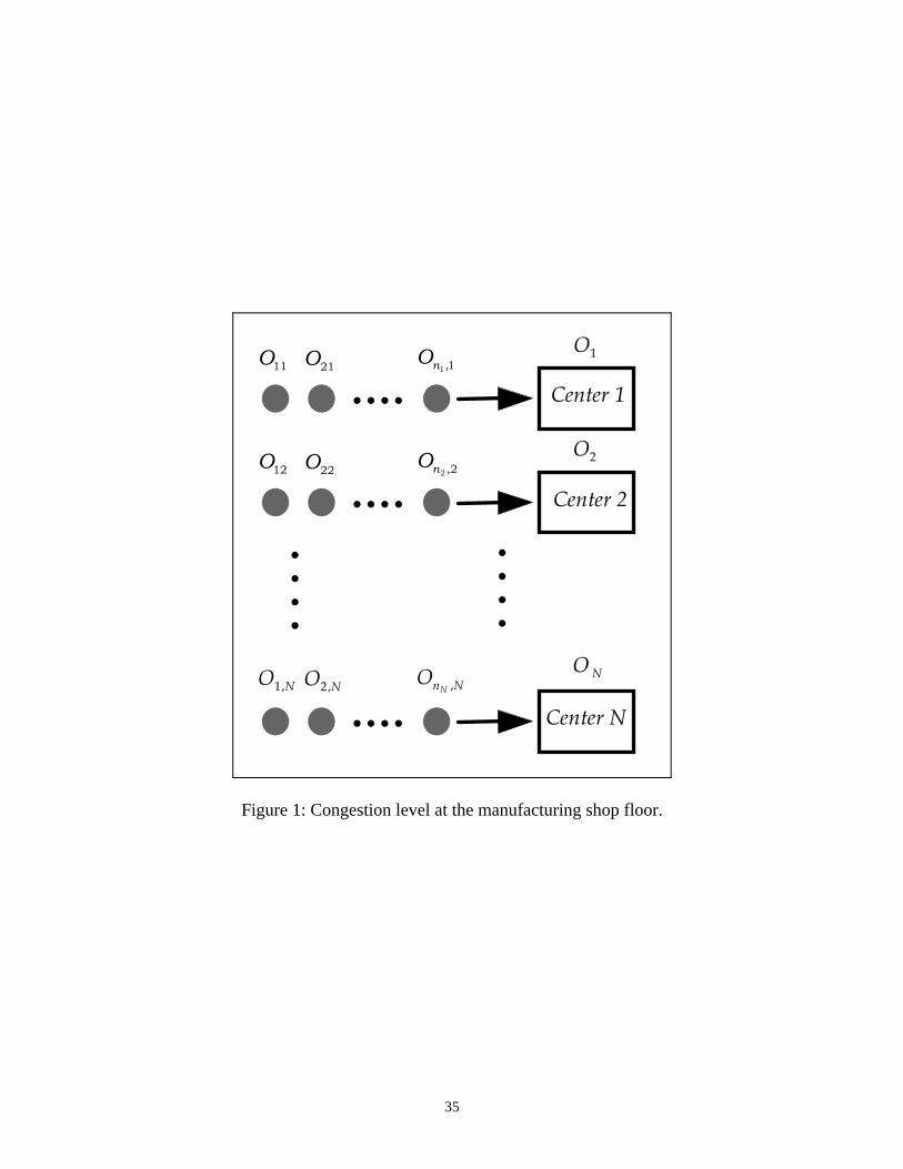
We consider a manufacturing system consisting of N processing centers that are subject to
random failures and repairs. We assume that the probability law of the failure process is known
in each center. Let Yj be the generic random variable of the sequence of down-times and Xj be
the generic random variable associated with the sequence of up-times when Center j is
processing a lot. Let F x X xX jj( ) Pr m r be the Cumulative Distribution Function (CDF) of Xj .
We assume that at the time a new order is to be placed by a customer, there are already
n njj
N
11c h scheduled lots (with N lots currently in-process). Here, nj represents the
5
number of lots queued at Center j. Let Oij i nj 1,2,...,c h be a lot consisting of qij units that are
waiting in queue to be processed at Center j. Lots O1, O2 , …, ON are the ones currently being
processed at centers 1 2, ,..., N , respectively (see Figure 1.). We assume that qj is the remaining
quantity to be processed from Lot Oj . Let Rij (rj , respectively) be the number of units that can
be processed from Lot Oij (Lot Oj , respectively) per unit of time at Center j. Notice that the lots
may be of different products. Let Sij represent the random variable denoting the setup time
needed to prepare Center j for the accommodation of Lot Oij . Let Uij (Uj , respectively) denote
the expected time it takes to manufacture the qij units of Lot Oij (the qj remaining units of Lot
Oj , respectively). Then, we have
U E S q R E Y M qij ij ij ij j j ij ( ). (1)
U q r E Y M qj j j j j j ( ). (2)
Here, E Yj is the expected repair or down-time of Center j, E Sij is the expected setup time for
Lot Oij at Center j, and M qj a fis the expected number of failures during the processing of a lot of
size q at Center j. Mj a f is the solution of the following integral equation
M q F q R M q x dF x Rj X X
q
j ja f a f a f z ( )
0. (3)
O11 O21On1 1,
Center 1
O1
O12 O22On2 ,2
Center 2
O2
O N1, O N2, On NN ,
Center N
O N
Figure 1: Congestion level at the manufacturing shop floor.
6
R is the processing speed of a particular order. The second part of Equation (1) (i.e. without the
expected setup time) was elegantly derived by Sivazlian [19]. For a lot of size q to be processed
at Center j, we define V qj a f to be the average inventory of unfinished work during the processing
of the q units. Then,
V qqR
E Y M u duqR
E Y M qj j j
q
j ja f a f a f FHG
IKJ FH IKz2
02. (4)
For completeness, a reproduction from Sivazlian [19] of the proof of Equations (2) and (4) is
provided in the appendix. Let I qj a f be the average inventory of finished work while processing q
units at Center j. Then, at any time, we have
I q V q qj ja f a f . (5)
Substituting V qj a f with its expression from Equation (4) and after mathematical manipulation,
we obtain
I q q R E Y um u du q R E Y M qj j j
q
j ja f a fe j a fe j z2
02( ) . (6)
Here,
m q dM q dqj j( ) ( ) . (7)
Where m qj ( ) represents the renewal density function of the failure times, while processing a lot
of size q at Center j. Notice that in the expressions of Uij , Uj , V qj a f and I qj a f, knowledge of the
CDF is only required for the up-times of a center. As an example, if failures occurred according
to a Poisson process with intensity j , E Yj j 1 and E S sij ij , then F x xX jj( ) exp 1 c h,
M q q Rj j( ) , m q Rj j( ) and hence,
U s q Rij ij ij j j ij 1 c h , (8)
V q I q qj ja f a f 2. (9)
This last result is expected because of the memoryless property of the exponential distribution of
the up-times. Notice in expression (8) that the term Rij j j1 c h represents the expected
processing rate of units from Lot Oij which is less than Rij .
Problem Statement: Consider a make-to-order system consisting of several processing centers
automated enough to accommodate all orders. Because of their non-homogeneity, the processing
7
centers incur different operating costs and exhibit different congestion levels over time.
Therefore, when an order is received, there are different options on how and when to
manufacture it. If the order is scheduled for processing on the most congested centers, then it
will be delivered late, which may not be satisfactory. On the other hand, if it is scheduled on the
least congested centers, then it will be delivered early, but this may result in a higher price. The
problem facing management is how to determine which centers to use to make this order, so as
to minimize the operating costs and assign a likely delivery date within a pre-specified time
window. In other words, how should management negotiate delivery date and price for an
upcoming order?
To answer the above question, let Q be the size of the order about to be placed and let x j be
the portion of it to be processed at Center j. x j is the decision variable representing the lot size to
be assigned to Center j. Then, we have
x Qjj
j N
1
. (10)
For Center j, let Sj denote the setup time, Aj denote the setup cost, cj denote the unit production
cost, and hj denote the unit inventory carrying cost of finished products per time unit. We
assume that the added value between the unfinished and finished products is an order of
magnitude higher. This assumption allows us to neglect the inventory carrying cost of unfinished
products. Let Wj denote the expected workload at Center j, then
W U Uj j ljl
l n j
1. (11)
Let Tj denote the expected processing time of lot x j at Center j, then
T E S x R E Y M xj j j j j j j ( ) . (12)
The expected completion time of lot x j at Center j is given by
CT W Tj j j . (13)
Let T denote the expected completion time of the entire order, then we have
T E Cj N
j LNMOQP
max,...,1m r . (14)
Here, Cj is the random variable associated with the completion time of lot x j at Center j. In
general, expression (14) is difficult to obtain analytically. To get around this problem, we are
8
going to adopt a conservative approach based on the following lemmas (All proofs are provided
in the appendix).
Lemma 1. Let Z Zj N
jmax
, ,1m r, where the Zj ’s are nonnegative random variables. Then, we have
E Z E Zj N
jmax
,...,1o t. (15)
Lemma 2. Referring to Lemma 1, the gap between the expected value of the maximum and the
maximum of the expected values is bounded by
( ( ) ( ))1
011N
F z F z dzj jj
N
j
N
z .
Applying Lemma 1. to our problem, we see that the maximum of the expected completion
times is less or equal to the expected maximum completion time. Therefore, we use
T Expected Completion Time of Center j CTj N j N
j max max
,..., ,...,1 1k p m r . (16)
According to Lemma 2., we expect the gap between the expected maximum completion time and
the maximum of the expected completion times to be very small for the following reasons: First,
usually the centers are typically very similar to each other. Therefore, they have similar
probabilistic characteristics with respect to setup, failure, and repair times. Second, as will be
shown later, an order may typically require considerably fewer centers than the total number of
available centers, and that the completion time of the chosen centers are very close to each
others. This leads to similar CDFs for the centers in question, resulting in a very small gap
between the expected maximum completion time and the maximum expected completion time of
the entire order. We demonstrate these issues in the computational experiences reported in
Section 6.
Equation (16) assumes that the whole order is to be delivered at once (i.e., no partial
deliveries), which is the case in most situations since partial deliveries involve extra shipping
and handling costs. Note that the order completion time is a function of the number of centers
used to manufacture the order and the lot sizes that make the order. The total operating cost
associated with the order about to be placed is then given by
f x T A x c x h I x T E S h x T T Wj j j j j j j j j j j j jj
j N( , ) ( ) ( )
e j c h1
. (17)
9
Here, x x x xN
T 1 2, ,...,b g and ( )x equals 1 if x 0 and 0, otherwise. The first term in
Expression (17) represents the setup cost incurred if Center j is to be used. The second term
represents the production cost at Center j. The third term represents the expected inventory
carrying cost while a lot is being produced at Center j. The last term represents the inventory
cost associated with a lot completed before the last lot is completed. The formal optimization
model can be written as follows
(P) Min A x c x h I x x x R E Y M x x T E S Wj j j j j j j j j j j j j j j jj
j N ( ) ( ) ( )
c he j e j{ }1 (18)
s.t.
x Qjj
j N
1
; (19)
W E S x x R E Y M x Tj j j j j j j j e j ( ) ( ) 0, j N 1, , ; (20)
T TU 0; (21)
T TL 0; (22)
x j 0 , j N 1, , ; T 0; (23)
Constraint set (20) assures that the order completion time is greater than the completion time
of the individual lots making up the order. Because we are minimizing, and because the
coefficient of T is positive, the delivery date will be equal to the completion time of the lot that is
completed last. In other words, at least one of the constraints in (20) will be binding at the
optimal solution. Constraint (21) makes sure that the order be completed no later than Time TU .
Constraint (22) makes sure that the order be completed no earlier than Time TL . Note that the
interval T TL U represents the pre-specified delivery window. Constraint set (23) represents the
usual non-negativity constraints. Notice that the latest order completion time can be obtained as
follows:
Latest Completion Time W E S Q R E Y M Qj N
j j j j j max ( )
, ,1o t. (24)
Problem (P) is formulated in a such a way that it can be used as a tool for either estimating or
negotiating the delivery date and price (operating cost plus a profit margin) of a certain order. In
the first case, by setting the value of TU to the latest order completion time, one obtains the
expected order completion time (through the values of the optimal lot sizes assigned to each
center) at the minimum operating cost. This case happens when a customer is willing to wait for
10
whatever time it is going to take for her order to be completed. In the second case, if a customer
is not satisfied with the initially estimated expected delivery date, an earlier delivery date can be
assigned to the variable TU and the optimization problem is solved again. Obviously, the
operating cost will increase. The incremental cost can be either partially or totally passed to the
customer depending on how important that customer is to the manufacturer. The negotiation
process continues until an agreement is reached. The lower bound on the order completion time,
TL , is added to make the model more general. This situation happens when a customer specifies a
time window for his order delivery date, to avoid having the order before it is needed. That is the
customer would like to receive his order no later than Time TU and no earlier than Time TL .
Before we proceed any further, a few comments are in order:
1. The above model optimizes only the operating cost of the current customer order and does
not take into account the effect of the assignment solution on the costs of future orders. The
reader may argue that accepting the current order may tie up the system and result in a longer
delivery date for a future order from a more important customer. This is not a limitation in
the context of the manufacturing systems we are considering. Indeed, these systems do not
reject any order. Further all the orders they receive have the same importance, and have to be
processed. In addition, because of the stochastic nature of the system, the model can be used
as often as possible to adjust the assignment of the workload in the system. As a
consequence, at the time a new order is placed, the model takes advantage of the most recent
and updated congestion level information. Furthermore, many manufacturers are reluctant to
reschedule already scheduled orders because of the nervousness introduced by such action
(Nahmias [16]), especially in a JIT production context, where raw materials are ordered
ahead of time so that they are received when needed.
2. It is extremely difficult to obtain the distribution of the completion time of the current order.
As a result, we are only using the expected value of the completion time as a promise for the
delivery date. To overcome this difficulty, we will determine the variance of the completion
time and use it to determine a safety margin to be added to the expected completion time of
the order.
3. The model does not incorporate a penalty if the order is delivered later than its promised
date. This is due to the fact that the agreed on delivery date will always be in the delivery
11
window specified by the customer (if the delivery window is feasible in the first place). The
actual delivery date may be later than the promised delivery date due to the stochastic nature
of the system. For this reason, we will add a safety margin to the completion time of the
order and use this as the promised delivery date of the order under consideration.
4. One of the goals of the proposed model is to reduce, or eliminate, the conflict between the
marketing/sales and production/manufacturing departments.
In the next section, we study a case that occurs commonly in practice, the case of an
impatient customer who would like to receive her order as soon as possible no matter what it
costs her. We will refer to impatient customers as time minimizing customers.
3. THE CASE OF A TIME MINIMIZING CUSTOMER
Let ( )P1 denote the problem of determining the earliest completion time possible. Problem
( )P1 can be formulated as follows
( )P1 Min g x TS( ) (25)
s.t.
x Qjj
j N
1
; (26)
W E S x x R E Y M x Tj j j j j j j j S e j ( ) ( ) 0 , j N 1, , ; (27)
x j 0 , j N 1, , ; TS 0; (28)
Here, TS denotes the earliest completion time. Notice that the cost is not relevant for this
problem. Before we proceed with the solution of Problem ( )P1 , we state the following
proposition.
Proposition 1. The function k x x R E Y M x c( ) ( ) , where c is a given constant, has at most
one zero in the interval 0,Q .
As an example, if the up times are exponentially distributed with parameter and the
expected repair time E Y 1, then k x x R c( ) 1 a f . If x* exists (Proposition 1), then
x cR* 1 a f. The following algorithm solves problem ( )P1 .
ALGORITHM TO SOLVE PROBLEM ( )P1
12
INITIALIZATION STEP
Sort the center indexes according to the increasing values of W E Sj je j, j N 1, , . Let
j N 1, , , be the indexing according to this sorting criterion. That is,
W E S W E S W E SN N1 1 2 2 c h c h c h. (29)
Set x j : 0 , j N 1, , , and set j: 1. Go to MAIN STEP.
MAIN STEP
For i j: : 1 , Solve the following equation for yi (using Proposition 1)
W E S y R E Y M y W E Si i i i i i i j j ( ) 1 1 ; (30)
Let
Q Q yii
i j
1.
If Q 0 , Then For i j: : 1 let x yi i: .
If j =N, Go to Termination step. Else, let j j: 1 and Got to Main step.
Else, le t
Q Q xii
i j
1 Termination step.
TERMINATION STEP
Solve the following system of nonlinear equations
y y y Q
y R E Y M y y R E Y M y
y R E Y M y y R E Y M y
j
j j j j j j j j j j
1 2
1 1 1 1 1 2 2 2 2 2
1 1 1 1 1
R
S||
T||
( ) ( )
( ) ( )
(31)
For i j: : 1 , let x x yi i i: ;
T W E S x R E Y M xS j j j j j j j ( ); (32)
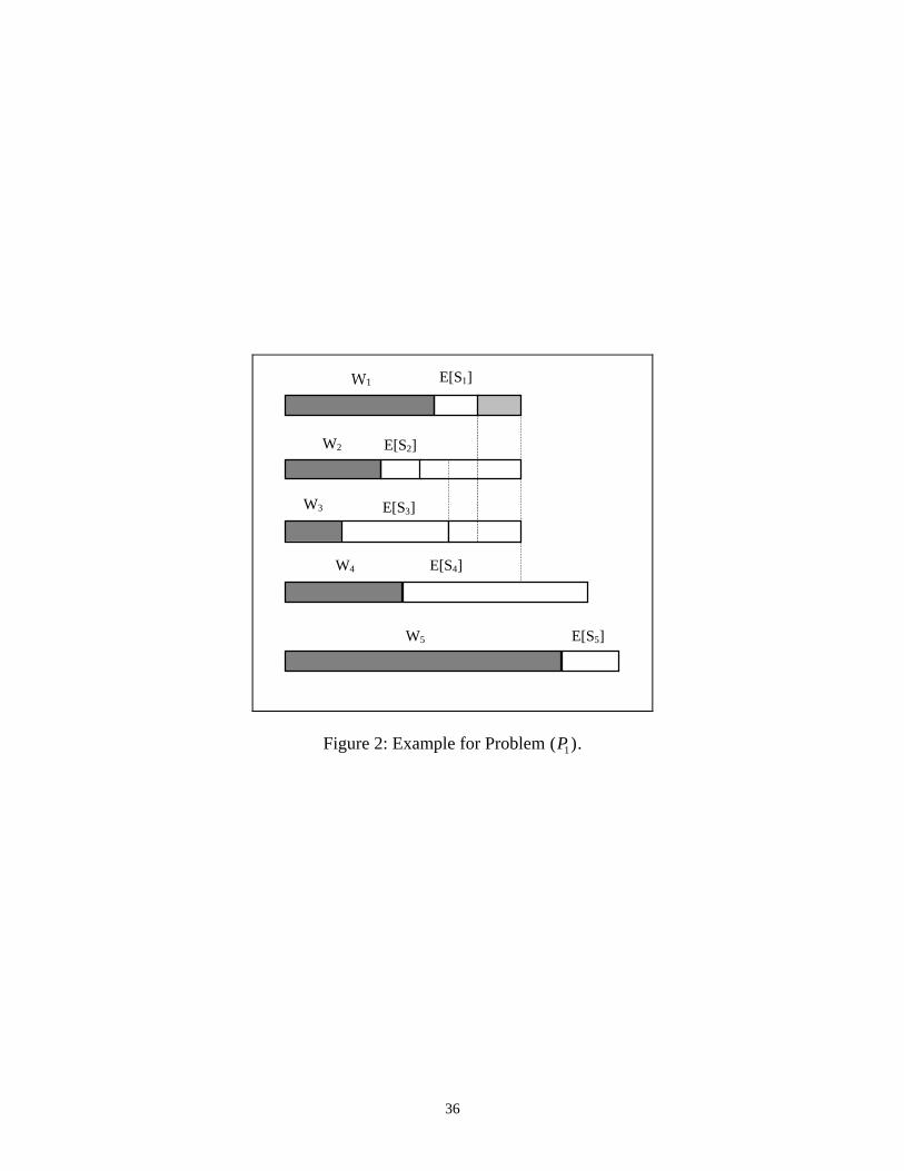
To be able to understand how the above algorithm works, consider the example of a
manufacturing system consisting of five processing centers. Figure 2 shows the workload Wj of
each center. The algorithm executes as follows: First, and since W E S2 2c h contains the
smallest such value, we find the quantity y1 that solves (30). Compute Q Q y1 0 and set
x y2 1 . Next, and since W E S3 3c h is the next smallest quantity, solve (30) once for y1 and
once for y2. Compute Q Q y y1 2 0 , set x y2 1 and x y3 2 . Next, solve (30) for y1, for y2
and for y3 . Compute Q Q y y y1 2 3 0 and set x y1 3 , x y2 1 , x y3 2 . Next, solve (30)
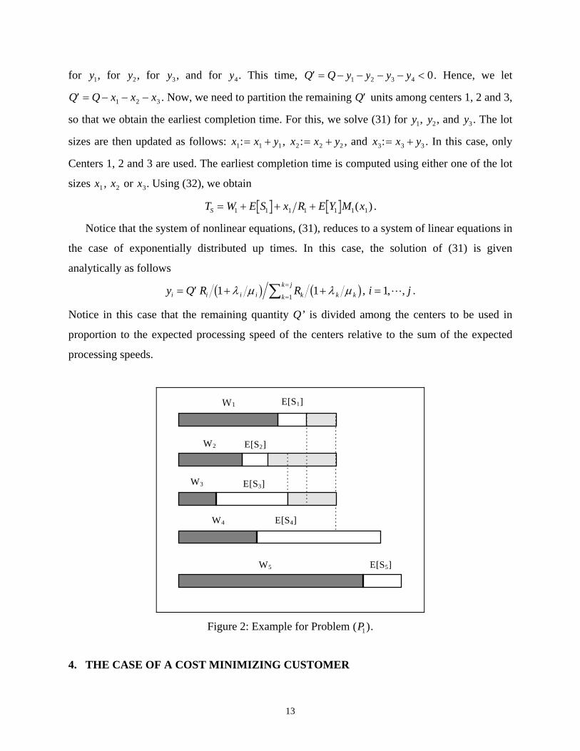
13
for y1, for y2, for y3 , and for y4. This time, Q Q y y y y1 2 3 4 0. Hence, we let
Q Q x x x1 2 3 . Now, we need to partition the remaining Q units among centers 1, 2 and 3,
so that we obtain the earliest completion time. For this, we solve (31) for y1, y2, and y3 . The lot
sizes are then updated as follows: x x y1 1 1: , x x y2 2 2: , and x x y3 3 3: . In this case, only
Centers 1, 2 and 3 are used. The earliest completion time is computed using either one of the lot
sizes x1 , x2 or x3. Using (32), we obtain
T W E S x R E Y M xS 1 1 1 1 1 1 1( ) .
Notice that the system of nonlinear equations, (31), reduces to a system of linear equations in
the case of exponentially distributed up times. In this case, the solution of (31) is given
analytically as follows
y Q R Ri i i i k k kk
k j
1 11
b g b g , i j 1, , .
Notice in this case that the remaining quantity Q’ is divided among the centers to be used in
proportion to the expected processing speed of the centers relative to the sum of the expected
processing speeds.
W1
W2
W4
E[S1]
E[S2]
W5 E[S5]
E[S4]
W3 E[S3]
Figure 2: Example for Problem ( )P1 .
4. THE CASE OF A COST MINIMIZING CUSTOMER
14
In this section, we study the case of customers who are willing to wait for their orders as long
as it takes so that they are quoted the lowest price. We assume that the centers have
exponentially distributed time to failure. The assumption on the breakdown distribution
represents systems with many unreliable sources or machines, each susceptible to breakdown
(Barlow and Proschan [4]). We make no assumption about the probability law of the repair and
setup times. Let j be the failure rate, E Yj j 1 be the expected repair time, and E S sj j
be the expected setup time at Center j. In this case, we have
M x x Rj j j j j( ) and I x xj j j( ) 2.
Substituting in (18) and rearranging terms, we obtain
f x T A x c h s W x h x T h R xj j j j j j j j j j j j j jj
j N, ( )a f c he j c he j{ }
1 2 2
1,
Substituting this expression in Problem (P), we obtain Problem (PE) which can be written as
follows
(PE) Min f x T A x c h T s W x h R xj j j j j j j j j j j jj
j N, ( ) ( )a f c he j c he j{ }
1 2 2
1 (33)
s.t.
x Qjj
j N
1
; (34)
W s x x R Tj j j j j j j c h c h ( ) 1 0, j N 1, , ; (35)
T TU 0; (36)
T TL 0; (37)
x j 0 , j N 1, , ; T 0; (38)
Notice that Problem (PE) is a mixed nonlinear 0-1 optimization problem with a nonlinear
objective function and linear constraints. Indeed, since we do not know which centers we are
going to use for the current order, the ( )'x sj are 0-1 decision variables as well. In general,
Problem (PE) is very difficult to solve. If T were fixed and we ignored the nonlinear terms of the
objective function, then the problem would reduce to the linear fixed-charge problem (see Murty
[15]). By employing an extreme-points ranking solution procedure, the number of vertices is
factorial in the number of constraints. This implies that a solution procedure may have to rank all
possible vertices before identifying the optimal vertex.
15
4.1 Solution Approach for Problem (PE)
In this section we outline an algorithm for finding an optimal solution to Problem (PE). To
be able to solve (PE), we first fix T, the completion time of the order to be placed. Now, since
we are fixing T, we only consider the centers with workload (including the setup time) less or
equal to T. In other words, we consider the centers that satisfy the following condition
( )W s Tj j , j N 1, , . (39)
Without loss of generality, assume that n n Na f centers satisfy condition (39) and that the
centers are re-indexed 1 2, , , n , accordingly. As a consequence of condition (39), constraint set
(35) holds for both cases ( )x j 1 and ( )x j 0, since
0 1 W s W s x R Tj j j j j j j j( ) , j n 1 2, , , .
Let
f x A x c h T s W x h R xj j j j j j j j j j j j j jc h c he j c he j ( ) ( )1 2 2 , j n 1 2, , , ; (40)
a R T W sj j j j j j c h c h1 , j n 1 2, , , ; (41)
Because the completion time is fixed, Constraints (36) and (37) can be ignored in Problem (PE).
The latter reduces to Problem PE(T) as follows
PE(T) Min f xj jj
j n( )
1 (42)
s.t.
x Qjj
j N
1
; (43)
0 x aj j , j n 1, , ; (44)
Notice that the objective function in Problem PE(T) is concave. Constraint (43) defines a
hyper-plane and constraint set (44) defines a hyper-rectangle, in n dimensional space. It is well
known that the minimum of a concave function always occurs at a vertex (see Horst et al. [13]).
To obtain the optimal solution to Problem PE(T), one evaluates the objective function at every
vertex and then picks the one that gives the minimum objective value. Fortunately, we do not
have to enumerate all the vertices of the polytope, D, generated by Constraints (43) and (44).
One of the earliest approaches, due to Murty [15], uses extreme point ranking and linear
underestimation. In our case, we notice that
F x x f a a f x f xj j j jj
j n
j jj
j n( ) ( ) ( ) ( )
1 1 x D . (45)
16
The latter states that the affine function F(x) underestimates the objective function of problem
PE(T). To see this, notice that each of the concave quadratics, f aj j: ,0 , can be
underestimated by the line connecting its two endpoints. Let v1 be an optimal solution to the
linear program
Min F xs t x D
( ). . (46)
Then, we have the following lower and upper bound for the optimal value f* of problem PE(T):
f F v f f v fl u ( ) * ( )1 1 . (47)
Therefore, starting from a solution v1 of LP (46), one can construct the ranking sequence by
determining the neighbors of v1 , then the neighbors of all the neighbors of v1 , and so on. The
adjacent vertices can be determined by simplex pivoting. The following algorithm guarantees an
optimal solution for problem PE(T) in a finite number of iterations. For more details, the reader
is referred to Horst et al. [13] (pages 82-83). The algorithm is based on an approach for extreme
point ranking due to Murty [15]. The algorithm is stated here for completeness.
4.2 Algorithm For Solving Problem PE(T)
Step 1: Solve the linear program (46) to obtain v1 and the lower bound f F vl ( )1 .
Step 2: Set v v f f vu 1, ( )
If F v fu( ) , then stop (v is optimal and f fu* ).
Step 3: Determine the first vector v2 in the ranking of the vertices of D with respect to F that
satisfies F v F v( ) ( )2 1 .
If f v fu( )2 , then set f f vu ( )2 , v v 2 .
If f v fu( )2 , then stop (v is optimal and f fu* ).
If F v fu( )2 and F v F v( ) ( )2 1 , then set f F vl ( )2 (improved lower bound).
Step 4: Set v v 2 and return to Step 3.
At this point a few comments are in order:
1. LP (46) does not require an LP solver for its optimal solution. Indeed, this problem is a
special version of the knapsack problem where the decision variables are continuous and
bounded. The optimal solution is obtained by a greedy procedure as follows: First, we sort
the cost coefficients in (46) in ascending order. Then, the decision variable associated with
17
the lowest cost is given its upper bound value (if Q is greater than the upper bound, otherwise
the decision variable is given the value Q). We continue this process, with the next lowest
cost coefficient, until the quantity Q is completely depleted.
2. Since the vertex ranking procedure requires simplex pivoting, we need to construct the
optimal simplex tableau of the solution of LP (46). Given the simple structure of the latter, its
simplex tableau is generated by inspection.
3. The vertex ranking procedure starts from the optimal vertex (with the minimum cost) and
moves to the next best vertex by pivoting in the same fashion as in the simplex method. The
method requires that the simplex tableaus of all generated vertices, so far, be stored so that
we make sure that we get the next best vertex at the next iteration. Since the constraint set in
LP (46) has coefficients that are either one or zero, the pivoting procedure requires additions
and subtractions only. This makes it very fast and efficient.
Let PE*(T) denote the optimal solution of problem PE(T) given a value of T. Unfortunately,
as will be shown later from the numerical examples, in general, PE(T) is neither concave nor
convex function of T. Furthermore PE(T) has several minima and maxima. Hence, T* cannot be
obtained using conventional line search techniques. Nonetheless, given the efficiency of the
above algorithms, we found that a simple sampling of the interval T TL U allows to obtain T* in
a relatively short amount of time. In addition, since the model is mainly going to be used as a
negotiation tool, it is more convenient to have the price (operating cost plus a profit margin)
variation of the order as a function of its likely completion time. The information could be
presented as a curve of the order price as a function of its completion time. The following
procedure summarizes the necessary steps to solve problem (PE).
4.3 Procedure for Solving Problem (PE)
Step 1: Determine TU using (24).
Determine TL using the algorithm for solving problem ( )P1 .
Let m be the number of sample points in T TL U .
Set T T T mU L b g , k 1, T Tk L .
Step 2: Solve PE Tk( ) using the algorithm for solving PE(T), and set C PE Tk k *( ).
18
Set k k 1.
If k > m go to Step 3.
If k m , set T T Tk k , go to Step 2.
Step 3: Set k Ck m
k* arg min, ,
1l q , C Ck* * , T Tk* * .
T* is the minimum cost completion time.
4.4 Numerical Examples
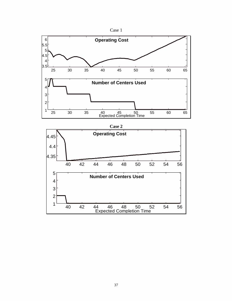
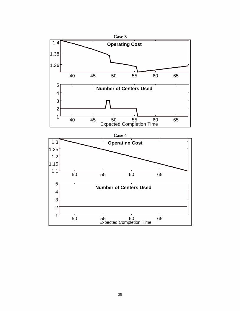
Figure 3 shows examples of the variation of the operating cost and the number of centers
used as a function of the expected completion time of the entire order. In all four Cases, the
manufacturing system consisted of five processing centers. As can be seen, the operating cost is
heavily dependent on the data of the system, mainly, the congestion at the shop floor. In general,
the operating cost is neither a convex nor a concave function of the expected completion time of
the order. The data sets for Cases 1 through 4 are generated according to the figures in Table 1
(see below). Case 1 is one where the inventory holding cost is high (up to 20% per day of the
production cost) compared to Cases 2 through 4. This is usually the case for make-to-order
systems, since by design these systems are not supposed to hold inventory either as WIP or
finished goods. Therefore, WIP/inventory is highly penalized in such systems. We also notice
that a relatively later expected completion time is not necessarily associated with lower operating
costs. The message here is that the shape of the operating cost function is highly dependent on
the underlying problem data. As a result, one has to be cautious when assigning a delivery date,
since it is possible to have a much higher operating cost just by moving the delivery date by a
few days (see e.g. Case 2 in Figure 3). Although this may seem counter-intuitive, it is important
to note that these graphs are generated by sampling the delivery window interval and then
computing the optimal assignment based on the fixed value of the completion time T.
5. DETERMINING A SAFETY MARGIN FOR THE DELIVERY DATE
In this section, we determine the variance of the completion time of the whole order based on
the splitting of the current order among the processing centers. As a result, the expression of the
variance of the completion time of an order is the same whether the customer is time minimizing
19
or cost minimizing. Here again, we assume that the time to failure of the different centers is
exponentially distributed.
20
Case 1
25 30 35 40 45 50 55 60 653.5
44.5
55.5
6
25 30 35 40 45 50 55 60 651
2
3
4
5
Expected Completion Time
Operating Cost
Number of Centers Used
Case 2
40 42 44 46 48 50 52 54 56
4.35
4.4
4.45
40 42 44 46 48 50 52 54 561
23
4
5
Expected Completion Time
Operating Cost
Number of Centers Used
Case 3
40 45 50 55 60 65
1.36
1.38
1.4
40 45 50 55 60 651
23
4
5
Expected Completion Time
Operating Cost
Number of Centers Used
Case 4
50 55 60 651.1
1.151.2
1.251.3
50 55 60 651
23
4
5
Expected Completion Time
Operating Cost
Number of Centers Used
Figure 3: Variation of the operating cost and the number of centers used as a function of the expected delivery date.
21
Proposition 2. The maximum variance, Vmax, of the completion time of the entire order is given
by
V Var S Var S Var Y x R q r q Rj N x
j ljl
n
j j j j j j j lj ljl
n
j
j j
max,
max
1 0 1
2
11
c h c h c he j{ } . (48)
Recall that our model uses only the expected value of the order completion time and ignores
its distribution; this may not be sufficient for assigning a reliable delivery date. One way to deal
with this is by adding a safety margin to the order completion time to obtain the delivery date to
be promised to the customer. Since the distribution of the actual completion time of the order is
not available, one may use Chebychev’s inequality, which states that
Pr T kk
l q 12
.
Here denotes the actual completion time of the order (r.v.), T denotes the expected completion
time of the order as determined by the model, and denotes the standard deviation of the
completion time of the order. For example when k 2, we are sure that there is at least 75%
chance that the actual completion time of the order will be within 2 of T. But, it has been
shown (Gosh and Meeden [14]) that Chebychev’s inequality is very conservative, and is almost
never attained. In other words, in most of the cases we can cover the same interval around the
mean with less number of standard deviation. This observation will be verified later in our
numerical experiments. In our case, we will use max instead of and we will show,
numerically, that for k 1 2 , there is at least 97% chance that the actual delivery date will not be
later than the quoted delivery date of T Tquoted 0 5. max . For k 1, we will show that there is at
least 99% chance that the actual delivery date will not be later than the quoted delivery date of
T Tquoted max . In other words, with k 1 2 , we achieve a minimum service level of 97%, and
with k 1, we achieve a minimum service level of 99%.
6. NUMERICAL EXPERIMENTS AND PERFORMANCES
In this section, we experiment with randomly generated data to assess the speed of the
proposed algorithm and more importantly, to assess the service level achieved by setting
different safety margins. But first, we present the data used in these experiments.
22
6.1 Experimental Data
The parameters used to generate the problem data sets are specified in Table 1. The
parameters in this table were used for all the numerical experiments, and have been drawn from a
uniform distribution U 3 3,c h , where represents the mean and represents the
standard deviation of the generated random numbers. In all cases, the standard deviation is
chosen to be 50% the value of the mean. Since, in this case, the uniform distribution is
completely specified by its mean, we only show the latter in Table 1.
Table 1: Experimental Data
Mean Time to Failure (1 j ) 20 days Centers Data
Mean Time to Repair (1 j ) 2 days
Number of lots queued at Center j: nj 5 lots
Quantity to be processed at Center j: qij 150 units
Processing speed at Center j: Rij 100 units/day
Queued Orders Data
Setup time at Center j: E Sij 2 days
Quantity to be processed at Center j: qj 75 units In-Process Orders Data Processing speed at Center j: rj 100 units/day
Setup cost at Center j: Aj $1000
Production cost at Center j: cj $50/unit
Holding cost at Center j: hj 0.25cj /year
Order size: Q 1000 units Processing speed at Center j: Rj 100 units/day
New Order Data
Setup time at Center j: E Sj 2 days
6.2 Algorithm’s Speed Performance
Since the proposed algorithm is mainly designed as a negotiation tool, where decisions have
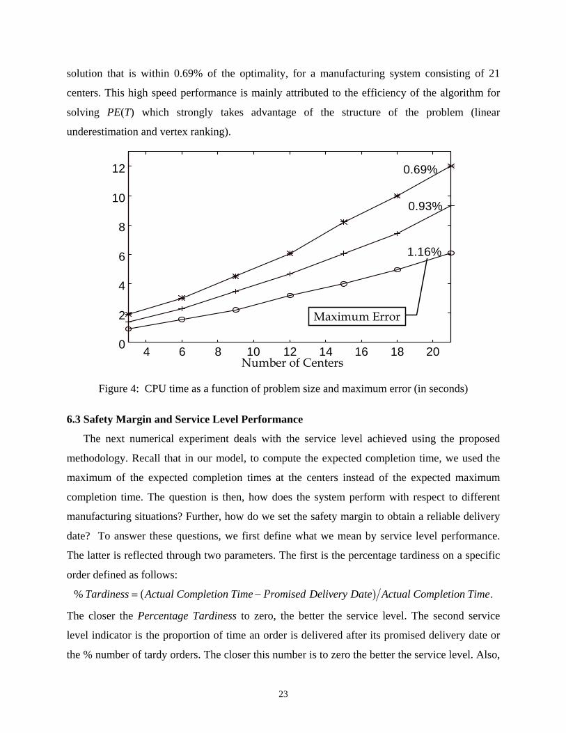
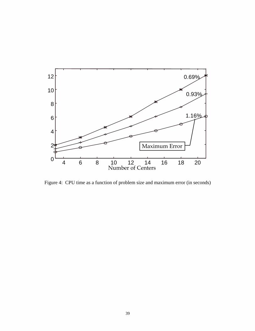
to be made in real-time, one is interested in the CPU time required to obtain a solution. Figure 4
shows the CPU run time to obtain the whole range of the expected completion time, as a
function of the number of centers in the manufacturing system1. The number next of each curve
represents the maximum error on the expected completion time (based on the earliest completion
time). As can be seen from Figure 4, the algorithm runs for about 12 seconds to deliver a
1 All procedures proposed in this paper were implemented in MatLab v. 4.2, and executed on a Pentium 166 MHz PC with 32 Mb of memory.
23
solution that is within 0.69% of the optimality, for a manufacturing system consisting of 21
centers. This high speed performance is mainly attributed to the efficiency of the algorithm for
solving PE(T) which strongly takes advantage of the structure of the problem (linear
underestimation and vertex ranking).
4 6 8 10 12 14 16 18 200
2
4
6
8
10
12
Number of Centers
0.69%
1.16%
0.93%
Maximum Error
Figure 4: CPU time as a function of problem size and maximum error (in seconds)
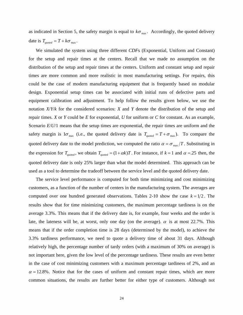
6.3 Safety Margin and Service Level Performance
The next numerical experiment deals with the service level achieved using the proposed
methodology. Recall that in our model, to compute the expected completion time, we used the
maximum of the expected completion times at the centers instead of the expected maximum
completion time. The question is then, how does the system perform with respect to different
manufacturing situations? Further, how do we set the safety margin to obtain a reliable delivery
date? To answer these questions, we first define what we mean by service level performance.
The latter is reflected through two parameters. The first is the percentage tardiness on a specific
order defined as follows:
% Tardiness Actual Completion Time omised Delivery Date Actual Completion Time Pra f .
The closer the Percentage Tardiness to zero, the better the service level. The second service
level indicator is the proportion of time an order is delivered after its promised delivery date or
the % number of tardy orders. The closer this number is to zero the better the service level. Also,
24
as indicated in Section 5, the safety margin is equal to k max . Accordingly, the quoted delivery
date is T T kquoted max .
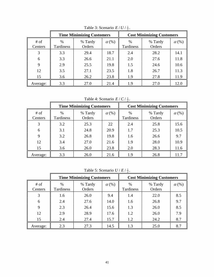
We simulated the system using three different CDFs (Exponential, Uniform and Constant)
for the setup and repair times at the centers. Recall that we made no assumption on the
distribution of the setup and repair times at the centers. Uniform and constant setup and repair
times are more common and more realistic in most manufacturing settings. For repairs, this
could be the case of modern manufacturing equipment that is frequently based on modular
design. Exponential setup times can be associated with initial runs of defective parts and
equipment calibration and adjustment. To help follow the results given below, we use the
notation X/Y/k for the considered scenarios: X and Y denote the distribution of the setup and
repair times. X or Y could be E for exponential, U for uniform or C for constant. As an example,
Scenario E/U/1 means that the setup times are exponential, the repair times are uniform and the
safety margin is 1 max (i.e., the quoted delivery date is T Tquoted max ). To compare the
quoted delivery date to the model prediction, we computed the ratio max T . Substituting in
the expression for Tquoted , we obtain T k Tquoted ( )1 . For instance, if k 1 and .25 then, the
quoted delivery date is only 25% larger than what the model determined. This approach can be
used as a tool to determine the tradeoff between the service level and the quoted delivery date.
The service level performance is computed for both time minimizing and cost minimizing
customers, as a function of the number of centers in the manufacturing system. The averages are
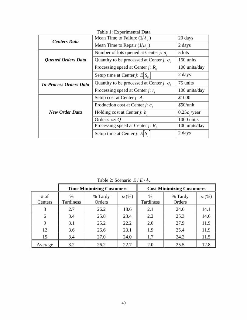
computed over one hundred generated observations. Tables 2-10 show the case k 1 2 . The
results show that for time minimizing customers, the maximum percentage tardiness is on the
average 3.3%. This means that if the delivery date is, for example, four weeks and the order is
late, the lateness will be, at worst, only one day (on the average). is at most 22.7%. This
means that if the order completion time is 28 days (determined by the model), to achieve the
3.3% tardiness performance, we need to quote a delivery time of about 31 days. Although
relatively high, the percentage number of tardy orders (with a maximum of 30% on average) is
not important here, given the low level of the percentage tardiness. These results are even better
in the case of cost minimizing customers with a maximum percentage tardiness of 2%, and an
12 8%. . Notice that for the cases of uniform and constant repair times, which are more
common situations, the results are further better for either type of customers. Although not
25
shown, we conducted the same numerical experiments with k 1 and found that for time
minimizing customers, the maximum percentage tardiness was 1.7%, was 22%, and the
maximum percentage number of tardy orders was 16%. For cost minimizing customers, we
found that the maximum percentage tardiness was 1%, was 13%, and the maximum
percentage number of tardy orders was 15%.
Based on the above extensive numerical results, we conclude that for time minimizing
customers, a safety margin of 1 2 max is sufficient to achieve an average service level of 97%
with a quoted delivery date that is only 11% larger than what the model determined. For cost
minimizing customers, a safety margin of 1 2 max is sufficient to achieve an average service
level of 98% with a quoted delivery date that is only 6% larger than what the model determined.
Table 2: Scenario E E/ / 12 .
Time Minimizing Customers Cost Minimizing Customers
# of Centers
% Tardiness
% Tardy Orders
(%) % Tardiness
% Tardy Orders
(%)
3 2.7 26.2 18.6 2.1 24.6 14.1
6 3.4 25.8 23.4 2.2 25.3 14.6
9 3.1 25.2 22.2 2.0 27.9 11.9
12 3.6 26.6 23.1 1.9 25.4 11.9
15 3.4 27.0 24.0 1.7 24.2 11.5
Average 3.2 26.2 22.7 2.0 25.5 12.8
Table 3: Scenario E U/ / 12 .
Time Minimizing Customers Cost Minimizing Customers
# of Centers
% Tardiness
% Tardy Orders
(%) % Tardiness
% Tardy Orders
(%)
3 3.3 29.4 18.7 2.4 28.2 14.1
6 3.3 26.6 21.1 2.0 27.6 11.8
9 2.9 25.5 19.8 1.5 24.6 10.6
12 3.5 27.1 23.5 1.8 26.7 11.3
15 3.6 26.2 23.8 1.9 27.8 11.9
Average: 3.3 27.0 21.4 1.9 27.0 12.0 Table 4: Scenario E C/ / 1
2 .
Time Minimizing Customers Cost Minimizing Customers
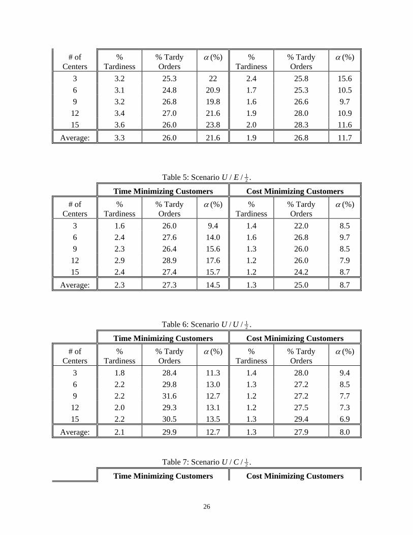
26
# of Centers
% Tardiness
% Tardy Orders
(%) % Tardiness
% Tardy Orders
(%)
3 3.2 25.3 22 2.4 25.8 15.6
6 3.1 24.8 20.9 1.7 25.3 10.5
9 3.2 26.8 19.8 1.6 26.6 9.7
12 3.4 27.0 21.6 1.9 28.0 10.9
15 3.6 26.0 23.8 2.0 28.3 11.6
Average: 3.3 26.0 21.6 1.9 26.8 11.7
Table 5: Scenario U E/ / 12 .
Time Minimizing Customers Cost Minimizing Customers
# of Centers
% Tardiness
% Tardy Orders
(%) % Tardiness
% Tardy Orders
(%)
3 1.6 26.0 9.4 1.4 22.0 8.5
6 2.4 27.6 14.0 1.6 26.8 9.7
9 2.3 26.4 15.6 1.3 26.0 8.5
12 2.9 28.9 17.6 1.2 26.0 7.9
15 2.4 27.4 15.7 1.2 24.2 8.7
Average: 2.3 27.3 14.5 1.3 25.0 8.7
Table 6: Scenario U U/ / 12 .
Time Minimizing Customers Cost Minimizing Customers
# of Centers
% Tardiness
% Tardy Orders
(%) % Tardiness
% Tardy Orders
(%)
3 1.8 28.4 11.3 1.4 28.0 9.4
6 2.2 29.8 13.0 1.3 27.2 8.5
9 2.2 31.6 12.7 1.2 27.2 7.7
12 2.0 29.3 13.1 1.2 27.5 7.3
15 2.2 30.5 13.5 1.3 29.4 6.9
Average: 2.1 29.9 12.7 1.3 27.9 8.0
Table 7: Scenario U C/ / 12 .
Time Minimizing Customers Cost Minimizing Customers
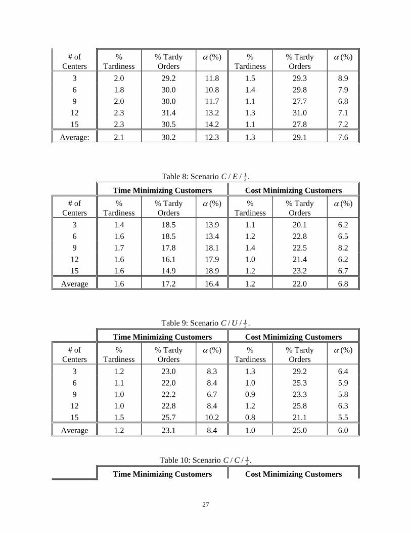
27
# of Centers
% Tardiness
% Tardy Orders
(%) % Tardiness
% Tardy Orders
(%)
3 2.0 29.2 11.8 1.5 29.3 8.9
6 1.8 30.0 10.8 1.4 29.8 7.9
9 2.0 30.0 11.7 1.1 27.7 6.8
12 2.3 31.4 13.2 1.3 31.0 7.1
15 2.3 30.5 14.2 1.1 27.8 7.2
Average: 2.1 30.2 12.3 1.3 29.1 7.6
Table 8: Scenario C E/ / 12 .
Time Minimizing Customers Cost Minimizing Customers
# of Centers
% Tardiness
% Tardy Orders
(%) % Tardiness
% Tardy Orders
(%)
3 1.4 18.5 13.9 1.1 20.1 6.2
6 1.6 18.5 13.4 1.2 22.8 6.5
9 1.7 17.8 18.1 1.4 22.5 8.2
12 1.6 16.1 17.9 1.0 21.4 6.2
15 1.6 14.9 18.9 1.2 23.2 6.7
Average 1.6 17.2 16.4 1.2 22.0 6.8
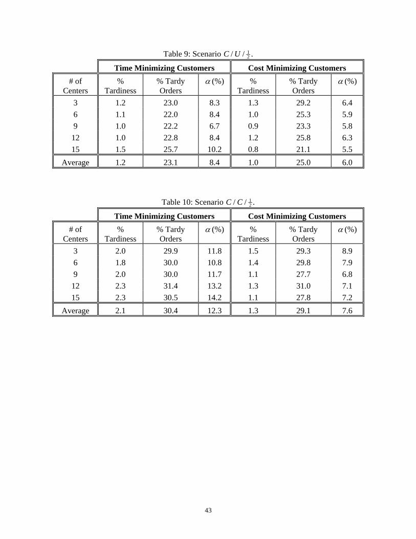
Table 9: Scenario C U/ / 12 .
Time Minimizing Customers Cost Minimizing Customers
# of Centers
% Tardiness
% Tardy Orders
(%) % Tardiness
% Tardy Orders
(%)
3 1.2 23.0 8.3 1.3 29.2 6.4
6 1.1 22.0 8.4 1.0 25.3 5.9
9 1.0 22.2 6.7 0.9 23.3 5.8
12 1.0 22.8 8.4 1.2 25.8 6.3
15 1.5 25.7 10.2 0.8 21.1 5.5
Average 1.2 23.1 8.4 1.0 25.0 6.0
Table 10: Scenario C C/ / 12 .
Time Minimizing Customers Cost Minimizing Customers
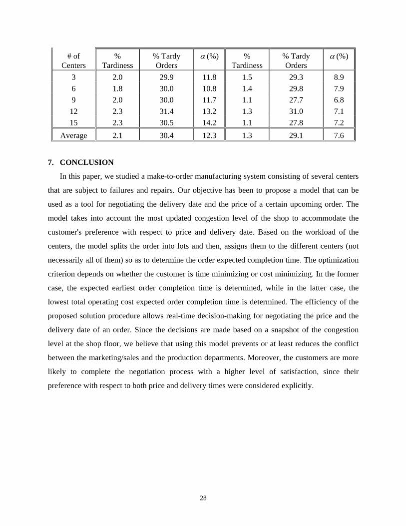
28
# of Centers
% Tardiness
% Tardy Orders
(%) % Tardiness
% Tardy Orders
(%)
3 2.0 29.9 11.8 1.5 29.3 8.9
6 1.8 30.0 10.8 1.4 29.8 7.9
9 2.0 30.0 11.7 1.1 27.7 6.8
12 2.3 31.4 13.2 1.3 31.0 7.1
15 2.3 30.5 14.2 1.1 27.8 7.2
Average 2.1 30.4 12.3 1.3 29.1 7.6
7. CONCLUSION
In this paper, we studied a make-to-order manufacturing system consisting of several centers
that are subject to failures and repairs. Our objective has been to propose a model that can be
used as a tool for negotiating the delivery date and the price of a certain upcoming order. The
model takes into account the most updated congestion level of the shop to accommodate the
customer's preference with respect to price and delivery date. Based on the workload of the
centers, the model splits the order into lots and then, assigns them to the different centers (not
necessarily all of them) so as to determine the order expected completion time. The optimization
criterion depends on whether the customer is time minimizing or cost minimizing. In the former
case, the expected earliest order completion time is determined, while in the latter case, the
lowest total operating cost expected order completion time is determined. The efficiency of the
proposed solution procedure allows real-time decision-making for negotiating the price and the
delivery date of an order. Since the decisions are made based on a snapshot of the congestion
level at the shop floor, we believe that using this model prevents or at least reduces the conflict
between the marketing/sales and the production departments. Moreover, the customers are more
likely to complete the negotiation process with a higher level of satisfaction, since their
preference with respect to both price and delivery times were considered explicitly.
29
REFERENCES
[1] Baker, K. R. (1984) Sequencing Rules and Due-date Assignments in a Job Shop.
Management Science, 30, 1093-1104.
[2] Baker, K. R. and Bertrand, J. W. M. (1981) An Investigation of Due-Date Assignment
Rules with Constrained Tightness. Journal of Operations Management, 1, 109-120.
[3] Baker, K. and Bertrand, J. W. M. (1981) A Comparison of Due-Date Selection Rules. AIIE
Transactions, 13, 123-131.
[4] Barlow, R. E. and Proschan, F. (1965) Mathematical Theory and Reliability, John Wiley &
Sons, NY.
[5] Bertrand, J. W. M. (1983) The Effect of Workload Dependent Due-dates on Job Shop
Performance. Management Science, 29, 799-816.
[6] Blackburn, J. (1991) Time Based Competition, Irwin, Homewood, IL.
[7] Bookbinder, J. H. and Noor, A. (1985) Setting Job-Shop Due-dates with Service-Level
Constraints. Journal of Operational Research Society, 36, 1017-1026.
[8] Chand, S. and Chhajed, D. (1992) A Single Model for Determination of Optimal Due Dates
and Sequence. Operations Research, 40, 596-602.
[9] Dudek, R. A., Panwalker S. S. and Smith M. L. (1992) The Lessons of Flowshop
Scheduling Research. Operations Research, 40, 7-13.
[10] Duenyas, I. (1995) Single Facility Due Date Setting with Multiple Customer Classes.
Management Science, 41, 608-619.
[11] Duenyas, I. and Hopp, W. J. (1995) Quoting Customer Lead Times. Management Science,
41, 43-57.
[12] Eilon, S. and Chowdhury I. G. (1976) Due Dates in Job Shop Scheduling. International
Journal of Production Research, 14, 223-237.
[13] Horst, R., Pardalos, P. M. and Thoai, N. V. (1995) Introduction to Global Optimization,
Kluwer Academic Publishers, Dordrecht, The Netherlands.
[14] Ghosh, M. and Meeden, G. (1977) On the Non-Attainability of Chebychev Bounds.
American Statistician, 31, 35-36.
[15] Murty, K. G. (1968) Solving the Fixed Charge Problem by Ranking the Extreme Points.
Operations Research, 16, 268-279.
[16] Nahmias, S. (1993) Production and Operations Management, Irwin, Homewood, IL.
30
[17] Seidmann, A. and Smith, M. L. (1981) Due Date Assignment for Production Systems.
Management Science, 27, 571-581.
[18] Shanthikumar, J. G. and Sumita, U. (1988) Approximations for the Time Spent in a
Dynamic Job Shop with Applications to Due-Date Assignment. International Journal of
Production Research, 26, 1329-1352.
[19] Sivazlian, B. D. (1992) The Filtered Counting Process and its Applications to Stochastic
Manufacturing Systems. Department of Industrial and Systems Engineering, University of
Florida, Research Report 92-13.
[20] Weeks, J. K. (1979) A Simulation Study of Predictable Due Dates. Management Science,
25, 363-373.
[21] Wein, L. (1991) Due-date Setting and Priority Sequencing in a Multiclass M/G/1 Queue.
Management Science, 37, 834-850.
[22] Wein, L., Whang, S. and Lemire, L. J. (1990) Due Date Setting and Pricing in a Single-
Server Queue. Sloan School of Management, M.I.T., Technical Report.
31
APPENDIX
Proof of Equations (2) and (4). (Reproduced from Sivazlian [19]).
For a particular center, let Xil q be the sequence of up times and Yil q the sequence of repair
times. The Xil q’s and Yil q’s are sequences of random variables mutually independent. Let
E X E Xi and E Y E Yi for all i. Let r denote the production rate which measures the
number of units produced/unit time. Let the random variable T rXi i denote the amount of work
completion in units during the ith uptime. Let Q denote the amount of work to be completed at
the center uninterruptedly. Then, N(Q) is the number of breakdowns until the total amount Q has
been completed. Since the Xil q’s are i.i.d., then the process N q q( ), 0k p is a renewal counting
process with the renewal function
M q E N q F q r M q u dF u rX
q( ) ( ) ( ) za f a f
0.
The total time to process the workload Q, U(Q), is given by
U QQ
rY Y YN Q( ) ( ) 1 2 .
Hence,
E U QQ
rE Y E N Q
Q
rE Y M Q( ) ( ) ( )a f
which proves Equation (2).
The cumulative unfinished work I(Q) at the center is given by
I QQ
rQ W Y Q W Y Q W YN Q N Q( ) ( ) ( )
2
1 1 2 22b g b g c h
where W T T Ti i 1 2 . Define the function w q W Y q W Yi i, , ( )b g . Then, the expected in-
process inventory is
E I QQ
rE w Q W Yi i
i
N Q
( ) , ,( )
LNM
OQP
2
12b g .
Define the indicator function
RSTq W Y w q W Y W qotherwisei i
i i i, , , ,b g b g 00
32
Also recall that E N q W qii
( ) Pr
l q1
. Then, assuming that the integrals are absolutely
convergent,
E I QQ
rE Q W Yi i
i
N Q
( ) , ,( )
LNM
OQP
2
12b g
Q
rE Q W Yi i
i
N Q2
12, ,
( )
b g
zzQ
rQ q u d W q dF ui Y
i
2
0012
, , Pr ( )a f l q
z zQ
rQ q u dF u d W qY i
i
2
01
02, , ( ) Pra f l q
z zQ
rw Q q u dF u d W qY i
i
Q2
01
02, , ( ) Pra f l q
zQ
rE w Q q Y dN q
Q2
02, , ( )a f
Recall that M q E N q( ) [ ( )] represents the expected number of breakdowns in the interval
0, qa when q units are processed. Let the rate of breakdown per processed unit be
m qd
dqE N q
dM q
dq( ) [ ( )]
( )
Then
E I QQ
rE Q q Y m q dq
Q( ) ( ) z2
02a f
zQ
rE Y Q q m q dq
Q2
02[ ] ( )a f
zQ
rE Y M q dq
Q2
02[ ] ( )
The average in-process inventory of unfinished work is
V QE I Q
E U Q
Q
rE Y M q dq
Qr
E Y M Q
Q
( )[ ( )]
[ ( )]
[ ] ( )
( )
z2
02
This proves Equation (4).
Proof of Lemma 1.
33
Since Z Zj , we have E Z E Zj , implying E Z E Zj max , j N 1, , .
Proof of Lemma 2.
E Z F z dz F z dz F z F z dz
E Z F z F z dz
k Nk j
j
N
j j jj
N
j j jj
N
max ( ( )) ( ( )) ( ( ) ( ))
( ( ) ( ))
, ,
LNM OQP
z z zz
11
0 01
0
10
1 1l q
Summing over all j’s, we obtain
NE Z E Z F z N F z dzk N
k jj
N
jj
N
jj
N
max ( ( ) ( )), ,
LNM OQP z11 1 1
0l q .
Since E Z E Zjk N
kmax
, ,1m r for all j’s, we have
NE Z N E Z F z N F z dzk N
kj N
j jj
N
jj
N
max max ( ( ) ( )), , , ,
LNM OQP z1 11 1
0 l q o t .
Dividing through by N and rearranging terms, we obtain
Gap E Z E ZN
F z F z dzk N
kj N
j j jj
N
j
N
LNM OQP
z max max ( ( ) ( ))
, , , ,1 1 011
1 l q o t .
Proof of Proposition 1.
It is clear that M x( ) is a monotonically increasing function of x over the interval 0,Q . Indeed,
the bigger the lot size, x, the higher the expected number of failures while producing the lot. It
follows that the function k x( ) is monotonically increasing over 0,Q . Now, if k Q( ) 0 , then
k x( ) has no zeros on 0,Q . On the other hand, if k Q( ) 0 , then there exists a unique x Q* , 0
such that k x( *) 0 .
Proof of Proposition 2.
Let j jx( ) be the random variable that denotes the completion time of a lot of size x j that is
assigned to Center j. Then,
j j j j iji
N q
lj lj lj iji
N q
l
n
j j j iji
N x
x q r Y S q R Y S x R Yj j j ljj j j
( )( ) ( ) ( )
FHG
IKJ FHG
IKJ FHG
IKJ
0 01 0
.
N qj ( ) represents the number of failures if a lot of size q is processed at Center j. The other
variables have the same meaning as before. The first term represents the processing time of the
34
in-process lot. The second term represents the processing time of all lots preceding lot x j and the
third term represents the processing time of lot x j itself.
Notice that Yiji
N qj
0
( )
has a compound Poisson distribution, since the time to failure of Center j
is exponentially distributed. Therefore, Var Y E N q Var Y Var N q E Yiji
N q
j j j j
j
FHGIKJ
0
2( )
( ) ( ) e j .
Since E N q Var N q qj j j( ) ( ) , where is the processing time at a center, it follows that
Var Y q Var Yiji
N q
j j j
j
FHGIKJ
0
21( )
e j .
The variance of j jx( ) is obtained by appropriately applying this last expression, noticing that
the processing times of the lots are statistically independent. The maximum variance of the
completion time of the order is then,
V Var S Var S Var Y x R q r q Rj N x
j ljl
n
j j j j j j j lj ljl
n
j
j j
max,
max
1 0 1
2
11
c h c h c he j{ } .
35
O11 O21 On1 1,
Center 1
O1
O12 O22 On2 ,2
Center 2
O2
O N1, O N2, On NN ,
Center N
O N
Figure 1: Congestion level at the manufacturing shop floor.
36
W1
W2
W4
E[S1]
E[S2]
W5 E[S5]
E[S4]
W3 E[S3]
Figure 2: Example for Problem ( )P1 .
37
Case 1
25 30 35 40 45 50 55 60 653.5
44.5
55.5
6
25 30 35 40 45 50 55 60 651
2
3
4
5
Expected Completion Time
Operating Cost
Number of Centers Used
Case 2
40 42 44 46 48 50 52 54 56
4.35
4.4
4.45
40 42 44 46 48 50 52 54 561
23
4
5
Expected Completion Time
Operating Cost
Number of Centers Used
38
Case 3
40 45 50 55 60 65
1.36
1.38
1.4
40 45 50 55 60 651
23
4
5
Expected Completion Time
Operating Cost
Number of Centers Used
Case 4
50 55 60 651.1
1.151.2
1.251.3
50 55 60 651
23
4
5
Expected Completion Time
Operating Cost
Number of Centers Used
39
4 6 8 10 12 14 16 18 200
2
4
6
8
10
12
Number of Centers
0.69%
1.16%
0.93%
Maximum Error
Figure 4: CPU time as a function of problem size and maximum error (in seconds)
40
Table 1: Experimental Data Mean Time to Failure (1 j ) 20 days
Centers Data Mean Time to Repair (1 j ) 2 days
Number of lots queued at Center j: nj 5 lots
Quantity to be processed at Center j: qij 150 units
Processing speed at Center j: Rij 100 units/day
Queued Orders Data
Setup time at Center j: E Sij 2 days
Quantity to be processed at Center j: qj 75 units In-Process Orders Data Processing speed at Center j: rj 100 units/day
Setup cost at Center j: Aj $1000
Production cost at Center j: cj $50/unit
Holding cost at Center j: hj 0.25cj /year
Order size: Q 1000 units Processing speed at Center j: Rj 100 units/day
New Order Data
Setup time at Center j: E Sj 2 days
Table 2: Scenario E E/ / 12 .
Time Minimizing Customers Cost Minimizing Customers
# of Centers
% Tardiness
% Tardy Orders
(%) % Tardiness
% Tardy Orders
(%)
3 2.7 26.2 18.6 2.1 24.6 14.1
6 3.4 25.8 23.4 2.2 25.3 14.6
9 3.1 25.2 22.2 2.0 27.9 11.9
12 3.6 26.6 23.1 1.9 25.4 11.9
15 3.4 27.0 24.0 1.7 24.2 11.5
Average 3.2 26.2 22.7 2.0 25.5 12.8
41
Table 3: Scenario E U/ / 12 .
Time Minimizing Customers Cost Minimizing Customers
# of Centers
% Tardiness
% Tardy Orders
(%) % Tardiness
% Tardy Orders
(%)
3 3.3 29.4 18.7 2.4 28.2 14.1
6 3.3 26.6 21.1 2.0 27.6 11.8
9 2.9 25.5 19.8 1.5 24.6 10.6
12 3.5 27.1 23.5 1.8 26.7 11.3
15 3.6 26.2 23.8 1.9 27.8 11.9
Average: 3.3 27.0 21.4 1.9 27.0 12.0
Table 4: Scenario E C/ / 12 .
Time Minimizing Customers Cost Minimizing Customers
# of Centers
% Tardiness
% Tardy Orders
(%) % Tardiness
% Tardy Orders
(%)
3 3.2 25.3 22 2.4 25.8 15.6
6 3.1 24.8 20.9 1.7 25.3 10.5
9 3.2 26.8 19.8 1.6 26.6 9.7
12 3.4 27.0 21.6 1.9 28.0 10.9
15 3.6 26.0 23.8 2.0 28.3 11.6
Average: 3.3 26.0 21.6 1.9 26.8 11.7
Table 5: Scenario U E/ / 12 .
Time Minimizing Customers Cost Minimizing Customers
# of Centers
% Tardiness
% Tardy Orders
(%) % Tardiness
% Tardy Orders
(%)
3 1.6 26.0 9.4 1.4 22.0 8.5
6 2.4 27.6 14.0 1.6 26.8 9.7
9 2.3 26.4 15.6 1.3 26.0 8.5
12 2.9 28.9 17.6 1.2 26.0 7.9
15 2.4 27.4 15.7 1.2 24.2 8.7
Average: 2.3 27.3 14.5 1.3 25.0 8.7
42
Table 6: Scenario U U/ / 12 .
Time Minimizing Customers Cost Minimizing Customers
# of Centers
% Tardiness
% Tardy Orders
(%) % Tardiness
% Tardy Orders
(%)
3 1.8 28.4 11.3 1.4 28.0 9.4
6 2.2 29.8 13.0 1.3 27.2 8.5
9 2.2 31.6 12.7 1.2 27.2 7.7
12 2.0 29.3 13.1 1.2 27.5 7.3
15 2.2 30.5 13.5 1.3 29.4 6.9
Average: 2.1 29.9 12.7 1.3 27.9 8.0
Table 7: Scenario U C/ / 12 .
Time Minimizing Customers Cost Minimizing Customers
# of Centers
% Tardiness
% Tardy Orders
(%) % Tardiness
% Tardy Orders
(%)
3 2.0 29.2 11.8 1.5 29.3 8.9
6 1.8 30.0 10.8 1.4 29.8 7.9
9 2.0 30.0 11.7 1.1 27.7 6.8
12 2.3 31.4 13.2 1.3 31.0 7.1
15 2.3 30.5 14.2 1.1 27.8 7.2
Average: 2.1 30.2 12.3 1.3 29.1 7.6
Table 8: Scenario C E/ / 12 .
Time Minimizing Customers Cost Minimizing Customers
# of Centers
% Tardiness
% Tardy Orders
(%) % Tardiness
% Tardy Orders
(%)
3 1.4 18.5 13.9 1.1 20.1 6.2
6 1.6 18.5 13.4 1.2 22.8 6.5
9 1.7 17.8 18.1 1.4 22.5 8.2
12 1.6 16.1 17.9 1.0 21.4 6.2
15 1.6 14.9 18.9 1.2 23.2 6.7
Average 1.6 17.2 16.4 1.2 22.0 6.8
43
Table 9: Scenario C U/ / 12 .
Time Minimizing Customers Cost Minimizing Customers
# of Centers
% Tardiness
% Tardy Orders
(%) % Tardiness
% Tardy Orders
(%)
3 1.2 23.0 8.3 1.3 29.2 6.4
6 1.1 22.0 8.4 1.0 25.3 5.9
9 1.0 22.2 6.7 0.9 23.3 5.8
12 1.0 22.8 8.4 1.2 25.8 6.3
15 1.5 25.7 10.2 0.8 21.1 5.5
Average 1.2 23.1 8.4 1.0 25.0 6.0
Table 10: Scenario C C/ / 12 .
Time Minimizing Customers Cost Minimizing Customers
# of Centers
% Tardiness
% Tardy Orders
(%) % Tardiness
% Tardy Orders
(%)
3 2.0 29.9 11.8 1.5 29.3 8.9
6 1.8 30.0 10.8 1.4 29.8 7.9
9 2.0 30.0 11.7 1.1 27.7 6.8
12 2.3 31.4 13.2 1.3 31.0 7.1
15 2.3 30.5 14.2 1.1 27.8 7.2
Average 2.1 30.4 12.3 1.3 29.1 7.6