systems

Article

A Generalized Stochastic Cost–Volume–Profit Model

Hongyan Liang 1,* , Alfred L. Guiffrida 2, Zilong Liu 3, Butje Eddy Patuwo 2 and Murali Shanker 2

�����������������

Citation: Liang, H.; Guiffrida, A.L.;

Liu, Z.; Patuwo, B.E.; Shanker, M. A

Generalized Stochastic

Cost–Volume–Profit Model. Systems

2021, 9, 81. https://doi.org/10.3390/

systems9040081

Academic Editor: Vladimír Bureš

Received: 28 September 2021

Accepted: 6 November 2021

Published: 11 November 2021

Publisher’s Note: MDPI stays neutral

with regard to jurisdictional claims in

published maps and institutional affil-

iations.

Copyright: © 2021 by the authors.

Licensee MDPI, Basel, Switzerland.

This article is an open access article

distributed under the terms and

conditions of the Creative Commons

Attribution (CC BY) license (https://

creativecommons.org/licenses/by/

4.0/).

1 Department of Business Administration, Gies College of Business, University of Illinois Urbana-Champaign,Champaign, IL 61820, USA

2 Ambassador Crawford College of Business and Entrepreneurship, Kent State University,Kent, OH 44240, USA; aguiffri@kent.edu (A.L.G.); epatuwo1@kent.edu (B.E.P.); mshanker@kent.edu (M.S.)

3 Discover Financial Service, Riverwoods, IL 60015, USA; zilongliu@discover.com* Correspondence: liangh@illinois.edu; Tel.: +1-217-300-7977

Abstract: Cost–volume–profit (CVP) analysis is a widely used decision tool across many businessdisciplines. The current literature on stochastic applications of the CVP model is limited in that themodel is studied under the restrictive forms of the Gaussian and Lognormal distributions. In thispaper we introduce the Mellin Transform as a methodology to generalize stochastic modeling ofthe CVP problem. We demonstrate the versatility of using the Mellin transform to model the CVPproblem, and present a generalization of the CVP model when the contribution margin and salesvolume are both defined by continuous random distributions.

Keywords: breakeven analysis; stochastic decision making; Mellin transform

1. Introduction

As a part of overall long-term business strategy, organizations are continually facedwith the task of deciding between competing alternatives. A wide range of decisionmodels exist to aid managers in evaluating and selecting the best alternative from a set ofcompeting alternatives [1–3]. The economic competitiveness of the global market coupledwith increased stakeholder concerns for environmental and social performance objectiveshas intensified the importance placed on the role played by management decision makingin the formulation of a firm’s core business strategy [4,5].

The scope of applications over which decision making is required is vast, coveringmultiple industry segments and numerous inter-firm and intra-firm value creating pro-cesses. Common to all these decision-making environments is the need to efficientlymanage information and knowledge; it is essential that decision makers understand theparadigms and systems that facilitate the collection, processing and analysis of informationand knowledge. This includes product–service (PPS) business models and their evaluationin decision-making support using key performance indicators [6], as well as the emergenceof decision-making schema within Industry 4.0 to improve decision making in such areas asoperations scheduling [7], sustainability [8], value chain reliability [9], and manufacturingand maintenance operations [10]. For a more in-depth investigation of this literature thereader is directed to the review articles of Pirola et al. [11], Xu et al. [12], and Lu [13].

When the decision under study requires the evaluation of profitability as a functionof output, cost–volume–profit (CVP) analysis is an attractive decision tool to use, since itenables managers to make decisions under business conditions where costs, revenue, andvolume are changing (see for example [14–16]). For situations involving a single product,decision makers can use CVP to determine the sales volume needed to achieve a targetedprofit when sales price, variable cost, or fixed cost change. When making decisions onestablishing and/or revising a product line, CVP analysis can also be used to identify themost profitable combination of products to include within the product line.

The CVP model has been studied for several decades, and applications of the modelstill prevail in practice at companies such as the Nestle Company Limited [17] and across a

Systems 2021, 9, 81. https://doi.org/10.3390/systems9040081 https://www.mdpi.com/journal/systems

Systems 2021, 9, 81 2 of 14

wide spectrum of organizations such as small businesses [18] and universities [19]. Despitethe widespread application of the CVP, two gaps exist in the literature with respect to theCVP model. First, the stochastic inputs of the model are restricted to either normal orlognormal distributions, resulting in profitability being modeled as a normal or lognormalrandom variable. In our opinion, normal and lognormal random variables are assumed onlyfor calculation simplicity. Second, when multiple stochastic inputs to the CVP model havebeen used, limiting assumptions have been used to simplify how the resulting probabilitydistribution representing profitability is defined.

To bridge these gaps, we propose a more generalized modeling of the stochastic CVPmodel that allows a wider range of candidate probability distributions for defining theinputs of the model. The novel feature of our modeling methodology is the introductionof the Mellin Transform technique as a means to generalize the stochastic modeling ofthe CVP model. For a gateway into the methodology of Mellin Transforms the readeris referred to Bertrand et al. [20] and Epstein [21]. Due to the unique properties of theMellin Transform, a much wider range of non-negative random variables can be usedin the formulation and analysis of stochastic CVP models. In addition, model structureswhere more than one input parameter is defined stochastically can be captured, moreaccurately representing the true underlying form of the model’s profitability distributionwhen multiple stochastic parameters exist. The research herein bridges the aforementionedgaps of the stochastic CVP model and contributes to supporting an expanded scope ofapplication for the model, as the model’s resulting profitability distribution (which wouldno longer have to be restricted to being normally or lognormally distributed) and multiplestochastic input parameters can be used. This extended scope of modeling flexibilityenhances the attractiveness and application of the model in decision-making environmentswhere uncertainty exists.

The remaining sections of this paper are organized as follows. In Section 2 we reviewthe literature on stochastic CVP models and identify limitations in the models. In Section 3we introduce the stochastic CVP model which uses the Mellin Transform methodology toovercome the limitations of the CVP models found in the literature, and conduct supportingnumerical analyses in order to illustrate the developed models. In Section 4 we present thesummary, conclusions and directions for future research.

2. Literature Review

In reality, uncertainty and risk exist and can therefore potentially affect each inputparameter of the CVP model. Hence, the deterministic CVP model defined in (1) is verylimited in its practical application. Jaedicke and Robichek [22] were the first to introducestochastic parameters into the CVP model, thus broadening the appeal and application ofthe model and establishing the baseline for the literature on stochastic CVP models.

Jaedicke and Robichek [22] were the first to integrate uncertainty into the CVP modelby defining profitability as a random variable under two different model formats. Inthe first model, sales volume is represented as a normally distributed random variable,while selling price, unit cost and fixed cost remain deterministic; in the second model,all four model inputs are defined as independent normally distributed random variables.In model one, expected profit T, which is a function of the combination of one normallydistributed random variable (sales Q) and three constants (selling price P, variable cost Vand fixed cost F), is normally distributed. In model two, the function defining expectedprofit T, which is defined by a function involving the difference of two normal randomvariables, (V − F), and the product of two normal random variables, Q × (P − V), isassumed to be normally distributed. While the difference of two independent normallydistributed random variables is well known in the literature to be normally distributed,the product of two independent normal random variables is not normally distributed andhas a relatively complicated distribution form Craig [23]. To simplify their model, Jaedickeand Robichek [22] assume that the product of two independent normal random variablesis normal. Under the normality assumption, the probability of gaining different levels of

Systems 2021, 9, 81 3 of 14

profits, including the probability of reaching the break-even level for competing productionalternatives, can be easy calculated using the model. This study provides the foundation tothe stochastic CVP model and its managerial application for selecting alternatives underconditions of uncertainty.

Ferrara et al. [24] point out the limitations in the model of Jaedicke and Robichek [22]and provide evidence from the literature that challenges the assumption made in Jaedickeand Robichek [22] that the product of two independent normal variables (Q and P − V) isalso a normal variable. They argue the assumption that the product of two independentnormally distributed random variables results in a normal distributed random variableholds only under certain conditions relating to the magnitude of the coefficients of variationof the random variables being multiplied. Using Monte Carlo simulation, they recommendthat if the sum of the coefficients of variation for unit sales Q times unit selling price Pminus variable cost V is less than or equal to 12 percent, the assumption that the productof two independent random variables, Q × (P − V), is also normally distributed can beaccepted at a 0.05 significance level.

Hilliard and Leitch [25] argue that the use of independent normally distributed ran-dom variables in a stochastic CVP model formulation in Jaedicke and Robichek [22] is toorigorous; the independent assumption is lack of practical support, since quantity, price,and variable cost are often correlated. Furthermore, under the normality assumption sales,prices, and variable costs can take on negative values when the standard deviation is large,which is problematic. Instead, they suggest that quantity and contribution margins arebivariate log-normal random variables and that dependent relationships obtain. Since theproduct of bivariate lognormal variables is known to be lognormal, Hilliard and Leitch [25]overcome the limitation faced by Jaedicke and Robichek [22]. However, the differencingof lognormal random variables continues to be a problem. To overcome this difficulty,Hilliard and Leitch [25] assume that the contribution margin as a whole is a lognormalvariable and the fixed variable is a constant.

Lau and Lau [26] argue that the input variables in a stochastic CPV analysis could beright skewed or left skewed, which is determined by some crucial factors. They posit thata symmetry assumption is better than the right skewness assumption, in that symmetryassumption includes the possibility of both right and left skewness. This work lessens thecontribution of Hilliard and Leitch [25] to some extent.

Jarrett [27] provides guidance for managers on how to use Bayesian Decision Theoryto estimate the parameters of the CVP. According to Jarrett [27], two options exist forparameter estimation: (i) use current information to guide all estimation, or (ii) postponeestimation until additional study on the parameters is completed. This paper also providespractical suggestions for managers to consider when selecting a given estimation option.

Kim [28] presents two modified CVP models intended to help financial analysts avoidthe problem of the difference of ex post and ex ante costs and prices in sensitivity analysis;some unexpected statistical and financial properties are displayed in this study.

Shih [29] points out the deficiency of the traditional CVP model in failing to distin-guish sales, demand and production. When production is larger than demand, the profitcalculated from the tradition CVP model is overestimated, especially when the unsoldproducts are perishable goods or the demand for the unsold products lasts only for acertain period of time. The tradition CVP model only includes the variable costs andfixed cost to produce the goods, not the costs to dispose of the leftovers. The traditionalCVP model is limited in its applicability when the sales, demands, and productions aredifferent. Shih [29] modifies the tradition CVP model to consider random demand anddetermined production. The modified model enables managers to make optimal decisionsunder uncertainty.

Systems 2021, 9, 81 4 of 14

Yunker [30] extends the traditional CVP model by incorporating the downward-sloping demand curve and the U-shaped average cost curve, which is more realistic thanShih (1979). The extended model demonstrates that a firm confronting uncertainty willproduce a smaller quantity than an equivalent firm under certainty, given a risk-aversemanager, while if the manager is risk-neutral, equivalent firms under uncertainty andcertainty will produce the same amount.

Cantrell and Ramsay [31] study the statistical properties of the target quantity estima-tor. The point estimate of target quantity is found to be biased, possessing no moments,but consistent. The interval estimate of target quantity is provided by using the Maximumlikelihood method for short-term and long-term analysis. This procedure minimizes theambiguity in the stochastic CVP model.

Kim et al. [32] incorporate the utility function of the decision maker into the CVPmodel. The authors argue that decisionmakers (managers) are trying their best to maximizetheir utility when they make decision on the investment in risky assets. Two main results arefound. First, a change in fixed costs affects not only the manager’s decision on production,but also the decision on risky assets. The highly risk-averse manager tends to invest more(less) in risky assets and less (more) in risk-free assets with increasing fixed costs. Second,for managers displaying constant absolute risk aversion, the optimal combination of riskyand risk-free assets is constant regardless of the changes in fixed costs. This study providessome insightful information on the managers’ investment behaviors.

Gonzalez [33] extends the single product CVP model into multiproduct CVP analysisthat is designed to be implemented at the enterprise level. The modified model requiresthe user to formulate a contribution rule that is consistent with the operating character-istics of the business environment as well as with the user’s assessment of the degree towhich the different products must contribute to recovering costs so as to meet a targetedprofitability level.

Lulaj and Iseni [34] show that the amount of product produced has a positive effecton sales value in service companies and increases profit in the manufacturing business en-vironment; there is also an important relationship between production and sales, and CVPanalysis contributes to growth profitability and break-even in the business environment.Therefore, cost–volume–profit analysis should be utilized to make judgments because therisk threshold is reduced by conducting CVP analysis.

In the context of multiproduct CVP analysis applications, Enyi [14] examines theefficacy of the Weighted Contribution Margin (WCM) with the Reversed ContributionMargin Ratio (RCMR). The WCM lacks analytical efficiency and generates suboptimalproduct mix because it ignores the inverse relationship between a product’s contributionmargin ratio (CMR) and its break-even point (BEP). The RCMR, which considers CMR/BEPtradeoff effects in its measurement, is recommended in the study.

Abdullahi et al. [18] examines the usage of CVP analysis as a decision-making tool insmall businesses. They find that small businesses use CVP incorrectly, and it is suggestedthat small businesses be exposed to CVP analysis and other management accountingtechniques in order to increase efficiency.

A review of the literature on stochastic CVP models identifies two key limitationsof the model. First, the stochastic inputs of the model are restricted to either normalor lognormal distributions. Second, in applications involving multiple stochastic inputsto the CVP model, limiting assumptions restrict the model. In Section 3, we present ageneralized stochastic CVP model which uses Mellin transform methodology to overcomethe limitations of the models found in the literature.

Systems 2021, 9, 81 5 of 14

3. Model Development3.1. CVP Model Definition and Assumptions

The basic CVP analysis involves the formulation of a total profit function for a singleproduct (see Equation (1)). Total profit is defined as total revenue minus total cost,

Z = Q × (P − V) − F (1)

where:Z = Total ProfitQ = Sales (in units)P = Selling price per unitV = Variable cost per unitF = Fixed cost.The objective is to determine the level of sales where total revenue equals total cost.

At this equilibrium, commonly referred to as the break-even point, the break-even quantityis defined as QBEP = F

P−V . When the sales volume is lower than QBEP a loss is incurred;when the sales volume is greater than QBEP a profit is generated.

When comparing across two competing alternatives, profit functions for each alterna-tive can be defined and the quantity level where the decisionmaker is indifferent betweenthe two alternatives can be determined. Given knowledge of this indifference point, thedecisionmaker can then determine for a projected sales level which alternative is mostprofitable.

The traditional CVP model is based on the following set of assumptions:

# Costs are only affected by a change in the sales level;# Costs (both variable and fixed) are linearly related to the sales level;# Revenues are linearly related to the sale level;# The inventory level is constant within a given time period;# All model parameters are deterministic.

3.2. Mathematical Transform Methods

In this section we provide the foundation of the Mellin transform which is usedas the key methodology for our development of a generalized stochastic CVP model.Mathematical transform methods are frequently used in operation research when solvingcomplex problems. Obtaining solutions by using transform methods is an indirect approachand can often avoid the complexity of using a direct solution procedure. Three transformmethods that are commonly used to analyze continuous functions are the Fourier, Laplace,and Mellin transforms. These transforms are particularly useful in defining and analyzingthe characteristic and moment generating functions of continuous random variables. Allcontinuous transforms are based on the Fourier transform. The Fourier, Laplace, and Mellintransforms are interchangeable, with each having advantages in different applications.

The Fourier transform (see Equation (2)) is well-known for deriving the probabilitydensities of sums and differences of random variables. If f (t) is a function of t, then Ft(u)is the Fourier transform of f (t). Ft(u) and f (t) form a unique transform pair, because Ft(u)uniquely defines f (t) and f (t) uniquely defines Ft(u).

Ft(u) =∫ ∞

−∞f (t)e−iutdt (2)

The Laplace transform is a derivative of the Fourier transform. If f (t) is a function oft, then L(s) is the Laplace transform of f (t) (see Equation (3)). L(s) and f (t) form a uniquetransform pair. The Laplace transform finds its most widespread application in solving

Systems 2021, 9, 81 6 of 14

differential equations. Laplace transforms are widely used in operations management andengineering due to well-developed transform pair tables.

L(s) =∫ ∞

−∞f (t)e−stdt (3)

If f (x) is a function of x, the Mellin transform of f (x) is defined by

FMx (s) =∫ ∞

0xs−1 f (x)dx (4)

The Mellin transform may also be defined for −∞ < x < ∞, but for applicationpurposes we focus only on the positive part. We note that f (x) and FMx (s) are uniquetransform pairs. The Mellin transform is a convenient technique for analyzing the productsand quotients of continuous random variables.

Let x1 and x2 be positive-valued continuous random variables with probability densityfunctions (pdf) of g(x1) and h(x2), respectively. Let x = x1x2, and let f (x) be the probabilitydensity function of x. Define FMx1

(s) and FMx2(s) as the Mellin transforms of g(x1) and

h(x2), respectively. The Mellin transform FMx (s) of f (x) is given by Schmidt and Davis [35]:

FMx (s) = FMx1(s)FMx2

(s) (5)

See Appendix A for the probability and cumulative probability density functions ofthe products of two random variables for the cases of the uniform, gamma and normalrandom variables.

If x = x1/x2, and f (x) is the probability density function of x, then the Mellintransform FMx (s) of f (x) is given by Schmidt and Davis [35]:

FMx (s) = FMx1(s)FMx2

(2− s) (6)

Similarly, if x = 1/x1, and f (x) is the probability density function of x, then the Mellintransform FMx (s) of f (x) is given by Schmidt and Davis [35]:

FMx (s) = FMx1(2− s) (7)

Schmidt and Davis [35] present the Mellin transform pairs for the most widely usedcontinuous random variables. Hence, the Mellin transforms of the products and quotientsof two continuous random variables can be easily obtained, given the Mellin transformsof the two random variables. Since the Mellin transform and the original function areuniquely paired, if we know the Mellin transform of the products or quotients of tworandom variables, we will find the probability density function by inverting the Mellintransform function. However, the product of two Mellin transforms is rarely any formatthat we can find the inverse function of; hence it is a challenge to find the pdf of the productsor quotients of two random variables. Nevertheless, like other continuous transforms,the Mellin transform can be used to compute the moments of random variables. FromEquation (7), we can get

FMx (s) = E(xs−1) (8)

This unique format of Mellin transform simplifies the process to find the nth momentof a continuous random variable. Replacing s with n + 1 in Equation (8) gives E(xn), thenth moment of random variable x, which is defined as

mn = FMx (n + 1). (9)

The first and second moments allow the definition of the mean and variance of arandom variable; the third and fourth moments can be used to determine the skewnessand excess kurtosis of the random variable. When it is difficult to find the exact pdf of a

Systems 2021, 9, 81 7 of 14

random variable, the key attributes of the random variable and its distributional form canbe estimated by studying the moments of the random variable.

3.3. Stochastic CVP Model

The stochastic CVP model has been studied for several decades. Applications of themodel still prevail in practice, and the attractiveness and usefulness of the model can beadvanced by further generalizing the model to bridge the following gaps. As identifiedin the review of the literature on the stochastic CVP model, the stochastic inputs of themodel are restricted to either normal or lognormal distributions, resulting in profitabilitybeing modeled as either a normal or lognormal random variable. In our opinion, normaland lognormal random variables are assumed only for the sake of calculation simplicity. Amore generalized distribution of profit in a stochastic CVP model that is not restricted tobeing normally or lognormally distributed can be obtained by using the Mellin Transformtechnique. The greater flexibility of selecting a wider range of different random variabletypes will enhance the application of the stochastic CVP model.

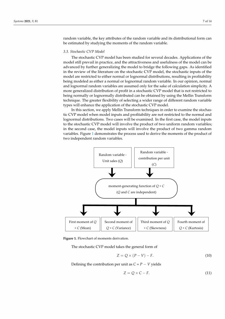
In this section, we apply Mellin Transform techniques in order to examine the stochas-tic CVP model when model inputs and profitability are not restricted to the normal andlognormal distributions. Two cases will be examined. In the first case, the model inputsto the stochastic CVP model will involve the product of two uniform random variables;in the second case, the model inputs will involve the product of two gamma randomvariables. Figure 1 demonstrates the process used to derive the moments of the product oftwo independent random variables.

Systems 2021, 9, x FOR PEER REVIEW 7 of 15

The first and second moments allow the definition of the mean and variance of a random variable; the third and fourth moments can be used to determine the skewness and excess kurtosis of the random variable. When it is difficult to find the exact pdf of a random variable, the key attributes of the random variable and its distributional form can be estimated by studying the moments of the random variable.

3.3. Stochastic CVP Model The stochastic CVP model has been studied for several decades. Applications of the

model still prevail in practice, and the attractiveness and usefulness of the model can be advanced by further generalizing the model to bridge the following gaps. As identified in the review of the literature on the stochastic CVP model, the stochastic inputs of the model are restricted to either normal or lognormal distributions, resulting in profitability being modeled as either a normal or lognormal random variable. In our opinion, normal and lognormal random variables are assumed only for the sake of calculation simplicity. A more generalized distribution of profit in a stochastic CVP model that is not restricted to being normally or lognormally distributed can be obtained by using the Mellin Transform technique. The greater flexibility of selecting a wider range of different random variable types will enhance the application of the stochastic CVP model.

In this section, we apply Mellin Transform techniques in order to examine the sto-chastic CVP model when model inputs and profitability are not restricted to the normal and lognormal distributions. Two cases will be examined. In the first case, the model in-puts to the stochastic CVP model will involve the product of two uniform random varia-bles; in the second case, the model inputs will involve the product of two gamma random variables. Figure 1 demonstrates the process used to derive the moments of the product of two independent random variables.

Figure 1. Flowchart of moments derivation.

The stochastic CVP model takes the general form of 𝑍 = 𝑄 × (𝑃 − 𝑉) − 𝐹. (10)

Defining the contribution per unit as C = P − V yields 𝑍 = 𝑄 × 𝐶 − 𝐹. (11)

First moment of Q

× C (Mean)

Second moment of

Q × C (Variance)

Third moment of Q

× C (Skewness)

Fourth moment of

Q × C (Kurtosis)

Random variable -

Unit sales (Q)

Random variable -

contribution per unit

(C)

moment-generating function of Q × C

(Q and C are independent)

Figure 1. Flowchart of moments derivation.

The stochastic CVP model takes the general form of

Z = Q× (P−V)− F. (10)

Defining the contribution per unit as C = P − V yields

Z = Q× C− F. (11)

Systems 2021, 9, 81 8 of 14

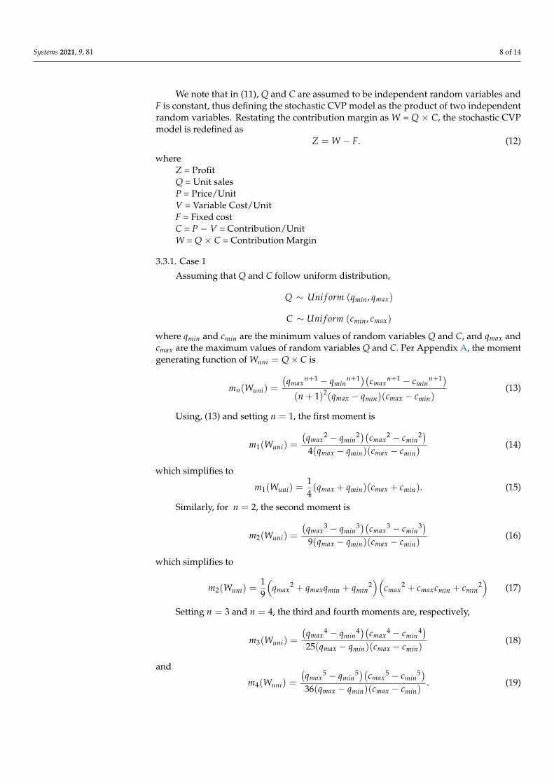
We note that in (11), Q and C are assumed to be independent random variables andF is constant, thus defining the stochastic CVP model as the product of two independentrandom variables. Restating the contribution margin as W = Q × C, the stochastic CVPmodel is redefined as

Z = W − F. (12)

whereZ = ProfitQ = Unit salesP = Price/UnitV = Variable Cost/UnitF = Fixed costC = P − V = Contribution/UnitW = Q × C = Contribution Margin

3.3.1. Case 1

Assuming that Q and C follow uniform distribution,

Q ∼ Uni f orm (qmin, qmax)

C ∼ Uni f orm (cmin, cmax)

where qmin and cmin are the minimum values of random variables Q and C, and qmax andcmax are the maximum values of random variables Q and C. Per Appendix A, the momentgenerating function of Wuni = Q× C is

mn(Wuni) =

(qmax

n+1 − qminn+1)(cmax

n+1 − cminn+1)

(n + 1)2(qmax − qmin)(cmax − cmin)(13)

Using, (13) and setting n = 1, the first moment is

m1(Wuni) =

(qmax

2 − qmin2)(cmax

2 − cmin2)

4(qmax − qmin)(cmax − cmin)(14)

which simplifies to

m1(Wuni) =14(qmax + qmin)(cmax + cmin). (15)

Similarly, for n = 2, the second moment is

m2(Wuni) =

(qmax

3 − qmin3)(cmax

3 − cmin3)

9(qmax − qmin)(cmax − cmin)(16)

which simplifies to

m2(Wuni) =19

(qmax

2 + qmaxqmin + qmin2)(

cmax2 + cmaxcmin + cmin

2)

(17)

Setting n = 3 and n = 4, the third and fourth moments are, respectively,

m3(Wuni) =

(qmax

4 − qmin4)(cmax

4 − cmin4)

25(qmax − qmin)(cmax − cmin)(18)

and

m4(Wuni) =

(qmax

5 − qmin5)(cmax

5 − cmin5)

36(qmax − qmin)(cmax − cmin). (19)

Systems 2021, 9, 81 9 of 14

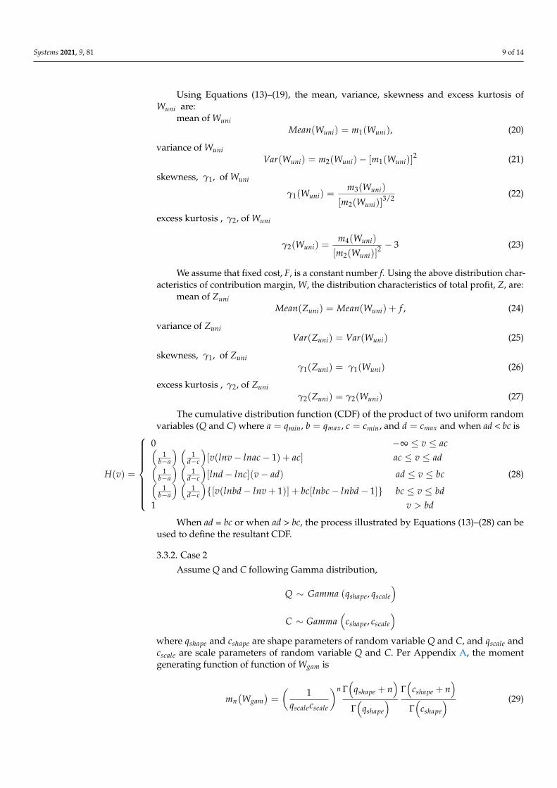
Using Equations (13)–(19), the mean, variance, skewness and excess kurtosis ofWuni are:

mean of WuniMean(Wuni) = m1(Wuni), (20)

variance of WuniVar(Wuni) = m2(Wuni)− [m1(Wuni)]

2 (21)

skewness, γ1, of Wuni

γ1(Wuni) =m3(Wuni)

[m2(Wuni)]3/2 (22)

excess kurtosis , γ2, of Wuni

γ2(Wuni) =m4(Wuni)

[m2(Wuni)]2 − 3 (23)

We assume that fixed cost, F, is a constant number f. Using the above distribution char-acteristics of contribution margin, W, the distribution characteristics of total profit, Z, are:

mean of ZuniMean(Zuni) = Mean(Wuni) + f , (24)

variance of ZuniVar(Zuni) = Var(Wuni) (25)

skewness, γ1, of Zuniγ1(Zuni) = γ1(Wuni) (26)

excess kurtosis , γ2, of Zuniγ2(Zuni) = γ2(Wuni) (27)

The cumulative distribution function (CDF) of the product of two uniform randomvariables (Q and C) where a = qmin, b = qmax, c = cmin, and d = cmax and when ad < bc is

H(v) =

0 −∞ ≤ v ≤ ac(1

b−a

) (1

d−c

)[v(lnv− lnac− 1) + ac] ac ≤ v ≤ ad(

1b−a

) (1

d−c

)[lnd− lnc](v− ad) ad ≤ v ≤ bc(

1b−a

) (1

d−c

){[v(lnbd− lnv + 1)] + bc[lnbc− lnbd− 1]} bc ≤ v ≤ bd

1 v > bd

(28)

When ad = bc or when ad > bc, the process illustrated by Equations (13)–(28) can beused to define the resultant CDF.

3.3.2. Case 2

Assume Q and C following Gamma distribution,

Q ∼ Gamma (qshape, qscale

)C ∼ Gamma

(cshape, cscale

)where qshape and cshape are shape parameters of random variable Q and C, and qscale andcscale are scale parameters of random variable Q and C. Per Appendix A, the momentgenerating function of function of Wgam is

mn(Wgam

)=

(1

qscalecscale

)n Γ(

qshape + n)

Γ(

qshape

) Γ(

cshape + n)

Γ(

cshape

) (29)

Systems 2021, 9, 81 10 of 14

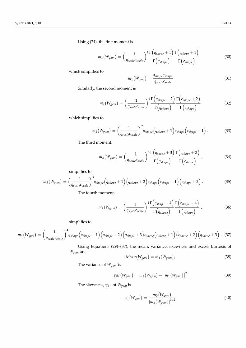
Using (24), the first moment is

m1(Wgam

)=

(1

qscalecscale

)1 Γ(

qshape + 1)

Γ(

qshape

) Γ(

cshape + 1)

Γ(

cshape

) (30)

which simplifies to

m1(Wgam

)=

qshapecshape.

qscalecscale(31)

Similarly, the second moment is

m2(Wgam

)=

(1

qscalecscale

)2 Γ(

qshape + 2)

Γ(

qshape

) Γ(

cshape + 2)

Γ(

cshape

) (32)

which simplifies to

m2(Wgam

)=

(1

qscalecscale

)2qshape

(qshape + 1

)cshape

(cshape + 1

). (33)

The third moment,

m3(Wgam

)=

(1

qscalecscale

)3 Γ(

qshape + 3)

Γ(

qshape

) Γ(

cshape + 3)

Γ(

cshape

) , (34)

simplifies to

m3(Wgam

)=

(1

qscalecscale

)3qshape

(qshape + 1

)(qshape + 2

)cshape

(cshape + 1

)(cshape + 2

). (35)

The fourth moment,

m4(Wgam

)=

(1

qscalecscale

)4 Γ(

qshape + 4)

Γ(

qshape

) Γ(

cshape + 4)

Γ(

cshape

) , (36)

simplifies to

m4(Wgam

)=

(1

qscalecscale

)4qshape

(qshape + 1

)(qshape + 2

)(qshape + 3

)cshape

(cshape + 1

)(cshape + 2

)(qshape + 3

). (37)

Using Equations (29)–(37), the mean, variance, skewness and excess kurtosis ofWgam are:

Mean(Wgam

)= m1

(Wgam

), (38)

The variance of Wgam is

Var(Wgam

)= m2

(Wgam

)−[m1(Wgam

)]2 (39)

The skewness, γ1, of Wgam is

γ1(Wgam

)=

m3(Wgam

)[m2(Wgam

)]3/2 (40)

Systems 2021, 9, 81 11 of 14

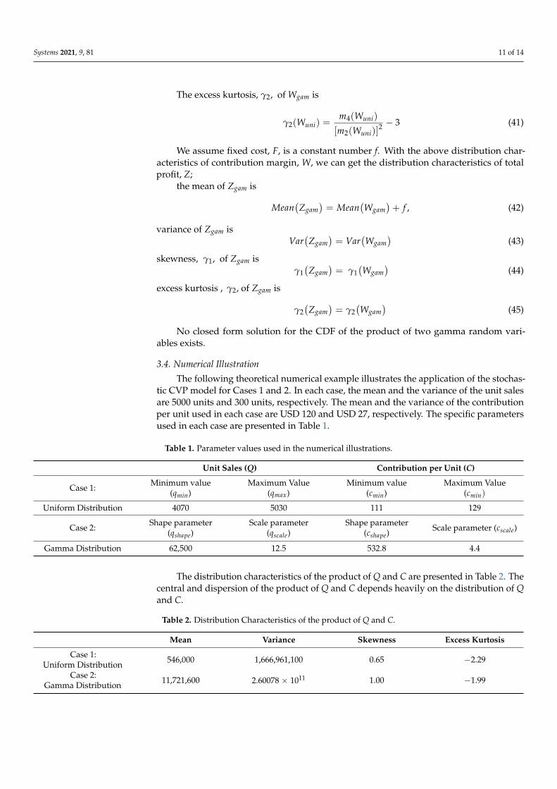
The excess kurtosis, γ2, of Wgam is

γ2(Wuni) =m4(Wuni)

[m2(Wuni)]2 − 3 (41)

We assume fixed cost, F, is a constant number f. With the above distribution char-acteristics of contribution margin, W, we can get the distribution characteristics of totalprofit, Z;

the mean of Zgam is

Mean(Zgam

)= Mean

(Wgam

)+ f , (42)

variance of Zgam isVar

(Zgam

)= Var

(Wgam

)(43)

skewness, γ1, of Zgam isγ1(Zgam

)= γ1

(Wgam

)(44)

excess kurtosis , γ2, of Zgam is

γ2(Zgam

)= γ2

(Wgam

)(45)

No closed form solution for the CDF of the product of two gamma random vari-ables exists.

3.4. Numerical Illustration

The following theoretical numerical example illustrates the application of the stochas-tic CVP model for Cases 1 and 2. In each case, the mean and the variance of the unit salesare 5000 units and 300 units, respectively. The mean and the variance of the contributionper unit used in each case are USD 120 and USD 27, respectively. The specific parametersused in each case are presented in Table 1.

Table 1. Parameter values used in the numerical illustrations.

Unit Sales (Q) Contribution per Unit (C)

Case 1: Minimum value(qmin)

Maximum Value(qmax)

Minimum value(cmin)

Maximum Value(cmin)

Uniform Distribution 4070 5030 111 129

Case 2: Shape parameter(qshape)

Scale parameter(qscale)

Shape parameter(cshape) Scale parameter (cscale)

Gamma Distribution 62,500 12.5 532.8 4.4

The distribution characteristics of the product of Q and C are presented in Table 2. Thecentral and dispersion of the product of Q and C depends heavily on the distribution of Qand C.

Table 2. Distribution Characteristics of the product of Q and C.

Mean Variance Skewness Excess Kurtosis

Case 1:Uniform Distribution 546,000 1,666,961,100 0.65 −2.29

Case 2:Gamma Distribution 11,721,600 2.60078 × 1011 1.00 −1.99

Systems 2021, 9, 81 12 of 14

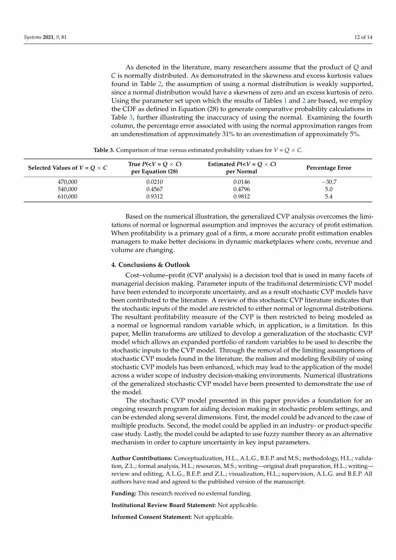
As denoted in the literature, many researchers assume that the product of Q andC is normally distributed. As demonstrated in the skewness and excess kurtosis valuesfound in Table 2, the assumption of using a normal distribution is weakly supported,since a normal distribution would have a skewness of zero and an excess kurtosis of zero.Using the parameter set upon which the results of Tables 1 and 2 are based, we employthe CDF as defined in Equation (28) to generate comparative probability calculations inTable 3, further illustrating the inaccuracy of using the normal. Examining the fourthcolumn, the percentage error associated with using the normal approximation ranges froman underestimation of approximately 31% to an overestimation of approximately 5%.

Table 3. Comparison of true versus estimated probability values for V = Q × C.

Selected Values of V = Q × C True P(<V = Q × C)per Equation (28)

Estimated P(<V = Q × C)per Normal Percentage Error

470,000 0.0210 0.0146 −30.7540,000 0.4567 0.4796 5.0610,000 0.9312 0.9812 5.4

Based on the numerical illustration, the generalized CVP analysis overcomes the limi-tations of normal or lognormal assumption and improves the accuracy of profit estimation.When profitability is a primary goal of a firm, a more accurate profit estimation enablesmanagers to make better decisions in dynamic marketplaces where costs, revenue andvolume are changing.

4. Conclusions & Outlook

Cost–volume–profit (CVP analysis) is a decision tool that is used in many facets ofmanagerial decision making. Parameter inputs of the traditional deterministic CVP modelhave been extended to incorporate uncertainty, and as a result stochastic CVP models havebeen contributed to the literature. A review of this stochastic CVP literature indicates thatthe stochastic inputs of the model are restricted to either normal or lognormal distributions.The resultant profitability measure of the CVP is then restricted to being modeled asa normal or lognormal random variable which, in application, is a limitation. In thispaper, Mellin transforms are utilized to develop a generalization of the stochastic CVPmodel which allows an expanded portfolio of random variables to be used to describe thestochastic inputs to the CVP model. Through the removal of the limiting assumptions ofstochastic CVP models found in the literature, the realism and modeling flexibility of usingstochastic CVP models has been enhanced, which may lead to the application of the modelacross a wider scope of industry decision-making environments. Numerical illustrationsof the generalized stochastic CVP model have been presented to demonstrate the use ofthe model.

The stochastic CVP model presented in this paper provides a foundation for anongoing research program for aiding decision making in stochastic problem settings, andcan be extended along several dimensions. First, the model could be advanced to the case ofmultiple products. Second, the model could be applied in an industry- or product-specificcase study. Lastly, the model could be adapted to use fuzzy number theory as an alternativemechanism in order to capture uncertainty in key input parameters.

Author Contributions: Conceptualization, H.L., A.L.G., B.E.P. and M.S.; methodology, H.L.; valida-tion, Z.L.; formal analysis, H.L.; resources, M.S.; writing—original draft preparation, H.L.; writing—review and editing, A.L.G., B.E.P. and Z.L.; visualization, H.L.; supervision, A.L.G. and B.E.P. Allauthors have read and agreed to the published version of the manuscript.

Funding: This research received no external funding.

Institutional Review Board Statement: Not applicable.

Informed Consent Statement: Not applicable.

Systems 2021, 9, 81 13 of 14

Data Availability Statement: Not applicable.

Acknowledgments: The authors sincerely thank the referees and editor for their valuable comments,which have directly contributed to the improvement of the clarity and contribution of this research.

Conflicts of Interest: The authors declare no conflict of interest.

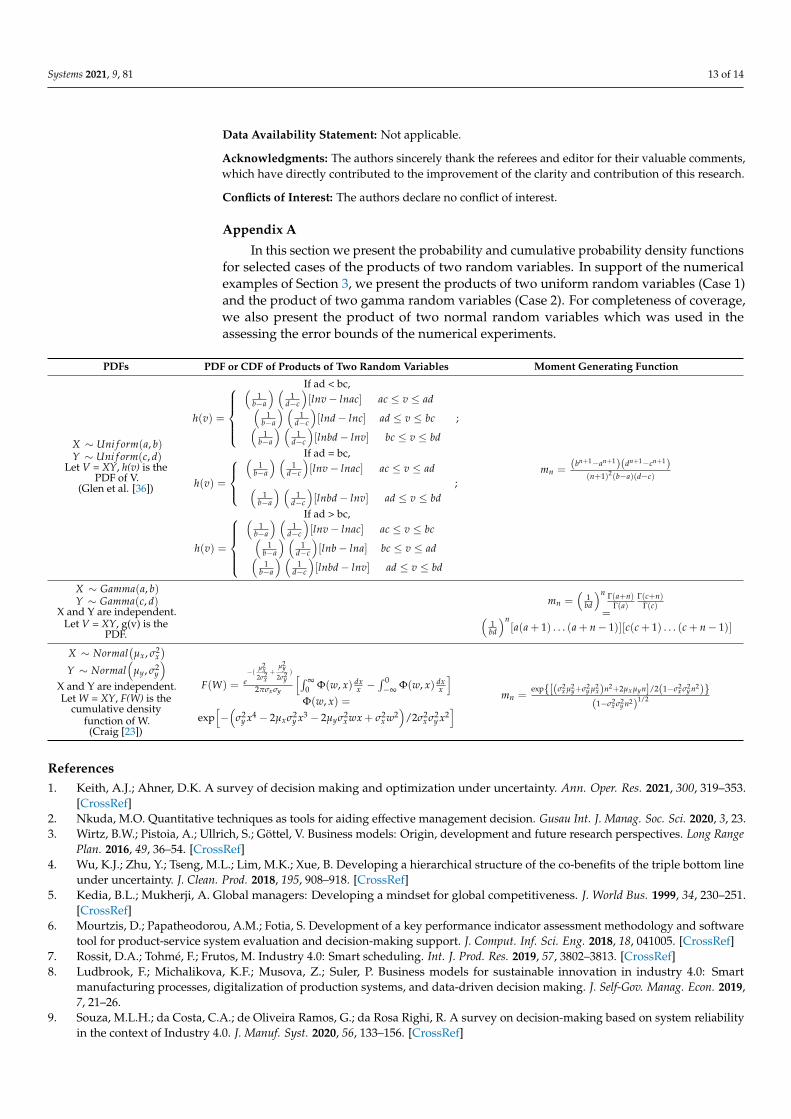
Appendix A

In this section we present the probability and cumulative probability density functionsfor selected cases of the products of two random variables. In support of the numericalexamples of Section 3, we present the products of two uniform random variables (Case 1)and the product of two gamma random variables (Case 2). For completeness of coverage,we also present the product of two normal random variables which was used in theassessing the error bounds of the numerical experiments.

PDFs PDF or CDF of Products of Two Random Variables Moment Generating Function

X ∼ Uni f orm(a, b)Y ∼ Uni f orm(c, d)

Let V = XY, h(v) is thePDF of V.

(Glen et al. [36])

If ad < bc,

h(v) =

(

1b−a

) (1

d−c

)[lnv− lnac] ac ≤ v ≤ ad(

1b−a

) (1

d−c

)[lnd− lnc] ad ≤ v ≤ bc(

1b−a

) (1

d−c

)[lnbd− lnv] bc ≤ v ≤ bd

;

If ad = bc,

h(v) =

(

1b−a

) (1

d−c

)[lnv− lnac] ac ≤ v ≤ ad(

1b−a

) (1

d−c

)[lnbd− lnv] ad ≤ v ≤ bd

;

If ad > bc,

h(v) =

(

1b−a

) (1

d−c

)[lnv− lnac] ac ≤ v ≤ bc(

1b−a

) (1

d−c

)[lnb− lna] bc ≤ v ≤ ad(

1b−a

) (1

d−c

)[lnbd− lnv] ad ≤ v ≤ bd

mn =(bn+1−an+1)(dn+1−cn+1)

(n+1)2(b−a)(d−c)

X ∼ Gamma(a, b)Y ∼ Gamma(c, d)

X and Y are independent.Let V = XY, g(v) is the

PDF.

mn =(

1bd

)n Γ(a+n)Γ(a)

Γ(c+n)Γ(c)

=(1bd

)n[a(a + 1) . . . (a + n− 1)][c(c + 1) . . . (c + n− 1)]

X ∼ Normal(µx , σ2

x)

Y ∼ Normal(

µy, σ2y

)X and Y are independent.Let W = XY, F(W) is the

cumulative densityfunction of W.

(Craig [23])

F(W) = e−( µ2

x2σ2

x+

µ2y

2σ2y)

2πσx σy

[∫ ∞0 Φ(w, x) dx

x −∫ 0−∞ Φ(w, x) dx

x

]Φ(w, x) =

exp[−(

σ2y x4 − 2µxσ2

y x3 − 2µyσ2x wx + σ2

x w2)

/2σ2x σ2

y x2] mn =

exp{[(σ2x µ2

y+σ2y µ2

x)n2+2µx µyn]/2(1−σ2x σ2

y n2)}(1−σ2

x σ2y n2)

1/2

References1. Keith, A.J.; Ahner, D.K. A survey of decision making and optimization under uncertainty. Ann. Oper. Res. 2021, 300, 319–353.

[CrossRef]2. Nkuda, M.O. Quantitative techniques as tools for aiding effective management decision. Gusau Int. J. Manag. Soc. Sci. 2020, 3, 23.3. Wirtz, B.W.; Pistoia, A.; Ullrich, S.; Göttel, V. Business models: Origin, development and future research perspectives. Long Range

Plan. 2016, 49, 36–54. [CrossRef]4. Wu, K.J.; Zhu, Y.; Tseng, M.L.; Lim, M.K.; Xue, B. Developing a hierarchical structure of the co-benefits of the triple bottom line

under uncertainty. J. Clean. Prod. 2018, 195, 908–918. [CrossRef]5. Kedia, B.L.; Mukherji, A. Global managers: Developing a mindset for global competitiveness. J. World Bus. 1999, 34, 230–251.

[CrossRef]6. Mourtzis, D.; Papatheodorou, A.M.; Fotia, S. Development of a key performance indicator assessment methodology and software

tool for product-service system evaluation and decision-making support. J. Comput. Inf. Sci. Eng. 2018, 18, 041005. [CrossRef]7. Rossit, D.A.; Tohmé, F.; Frutos, M. Industry 4.0: Smart scheduling. Int. J. Prod. Res. 2019, 57, 3802–3813. [CrossRef]8. Ludbrook, F.; Michalikova, K.F.; Musova, Z.; Suler, P. Business models for sustainable innovation in industry 4.0: Smart

manufacturing processes, digitalization of production systems, and data-driven decision making. J. Self-Gov. Manag. Econ. 2019,7, 21–26.

9. Souza, M.L.H.; da Costa, C.A.; de Oliveira Ramos, G.; da Rosa Righi, R. A survey on decision-making based on system reliabilityin the context of Industry 4.0. J. Manuf. Syst. 2020, 56, 133–156. [CrossRef]

Systems 2021, 9, 81 14 of 14

10. Bousdekis, A.; Lepenioti, K.; Apostolou, D.; Mentzas, G. A review of data-driven decision-making methods for Industry 4.0maintenance applications. Electronics 2021, 10, 828. [CrossRef]

11. Pirola, F.; Boucher, X.; Wiesner, S.; Pezzotta, G. Digital technologies in product-service systems: A literature review and a researchagenda. Comput. Ind. 2020, 123, 103301. [CrossRef]

12. Xu, L.D.; Xu, E.L.; Li, L. Industry 4.0: State of the art and future trends. Int. J. Prod. Res. 2018, 56, 2941–2962. [CrossRef]13. Lu, Y. Industry 4.0: A survey on technologies, applications and open research issues. J. Ind. Inf. Integr. 2017, 6, 1–10. [CrossRef]14. Enyi, E.P. Joint Products CVP Analysis–Time for Methodical Review. J. Econ. Bus. 2019, 2, 1288–1297. [CrossRef]15. Braun, K.W.; Tietz, W.M. Managerial Accounting; Pearson Education: New York, NY, USA, 2013.16. Adar, Z.; Barnea, A.; Lev, B. A comprehensive cost-volume-profit analysis under uncertainty. Account. Rev. 1977, 52, 137–149.17. Navaneetha, B.N.; Punitha, K.P.; Joseph, R.M.; Rashmi, S.R.; Aishwariyaa, T.S. An analysis of cost volume profit of Nestlé Limited.

Manag. Adm. Sci. Rev. 2017, 6, 99–103.18. Abdullahi, S.R.; Bello, S.; Mukhtar, I.S.; Musa, M.H. Cost-volume-profit analysis as a management tool for decision making in

small business enterprise within Bayero university, Kano. Iosr J. Bus. Manag. 2017, 19, 40–45. [CrossRef]19. Le, O.T.T.; Tran, P.T.T.; Tran, T.V.; Nguyen, C.V. Application of cost-volume-profit analysis in decision-making by public

universities in Vietnam. J. Asian Financ. Econ. Bus. 2020, 7, 305–316. [CrossRef]20. Bertrand, J.; Bertrand, P.; Ovarlez, J. The Mellin Transform. In The Transforms and Applications Handbook, 2nd ed.; Poularikas, A.D.,

Ed.; CRC Press: Boca Raton, FL, USA, 2000.21. Espstein, B. Some applications of the Mellin transform in statistics. Ann. Math. Stat. 1948, 19, 370–379. [CrossRef]22. Jaedicke, R.K.; Robichek, A.A. Cost-volume-profit analysis under conditions of uncertainty. Account. Rev. 1964, 39, 917–926.23. Craig, C.C. On the frequency function of xy. Ann. Math. Stat. 1936, 7, 1–15. [CrossRef]24. Ferrara, W.L.; Hayya, J.C.; Nachman, D.A. Normalcy of profit in the Jaedicke-Robichek Model. Account. Rev. 1972, 47, 299–307.25. Hilliard, J.E.; Leitch, R.A. Cost-volume-profit analysis under uncertainty: A log normal approach. Account. Rev. 1975, 50, 69–80.26. Lau AH, L.; Lau, H.S. CVP analysis under uncertainty—A log normal approach: A Comment. Account. Rev. 1976, 50, 163–167.27. Jarrett, J.E. An approach to Cost-Volume-Profit analysis under uncertainty. Decis. Sci. 1973, 4, 405–420. [CrossRef]28. Kim, C. A stochastic cost volume profit analysis. Decis. Sci. 1973, 4, 329–342. [CrossRef]29. Shih, W. A general decision model for cost-volume-profit analysis under uncertainty. Account. Rev. 1979, 54, 687–706.30. Yunker, J.A. Stochastic CVP analysis with economic demand and cost functions. Rev. Quant. Financ. Account. 2001, 17, 127–149.

[CrossRef]31. Cantrell, R.S.; Ramsay, L.P. Some statistical issue in the estimation of a simple Cost-Volume-Profit model. Decis. Sci. 1984, 15,

507–521. [CrossRef]32. Kim, S.; Abdolmohammadi, M.J.; Klein, L.A. CVP under uncertainty and the manager’s utility function. Rev. Quant. Financ.

Account. 1996, 6, 133–147. [CrossRef]33. González, L. Multiproduct CVP analysis based on contribution rules. Int. J. Prod. Econ. 2001, 73, 273–284. [CrossRef]34. Lulaj, E.; Iseni, E. Role of analysis CVP (Cost-Volume-Profit) as important indicator for planning and making decisions in the

business environment. Eur. J. Econ. Bus. Stud. 2018, 4, 99–114. [CrossRef]35. Schmidt, J.W.; Davis, R.P. Foundations of Analysis in Operations Research; Academic Press, Inc.: Cambridge, MA, USA, 1981.36. Glen, A.G.; Leemis, L.M.; Drew, J.H. Computing the distribution of the product of two continuous random variables. Comput.

Stat. Data Anal. 2004, 44, 451–464. [CrossRef]