Inflation and welfare in a stochastic production economy
16
The Quarterly Review of Economics and Finance, Vol. 36, No. 1, Spring, 1996, pages 1-16 Copyright 0 1996 Trustees of the University of Illinois All rights of reproduction in any form reserved ISSN 1062-9769 Inflation and Welfare in a Stochastic Production Economy Nivedita Mukherji Oakland University This pqtwr analyzes the relationshtp betuwn money and labor supply, and derives money’s opti- mal rate of ~‘etwn when production fiuzctions experience stochastic shocks. Inrwases in money’s return incwase both the dvtermwustx component and vannnce of labor s~~pply. Mowow~, money’s optimal rate is found to diffPr from both, the late suggested by Friedman and the. rates suggested by others for stochnstzc but pure endowment economies. Optimal policy is either in@- tumuly or dejlationaty depending on pawuwteGation. I. INTRODUCTION Friedman proposed in his seminal 1969 article, “The Optimum Quantity of Money,” that individuals should not economize on holding money, a socially costless asset. In an economy with alternative assets, superneutral money, and no distortions such as taxes or legal restrictions, money should be deflated at the real rate of interest to eliminate interest rate differentials between money and alternative assets. While Friedman’s proposition has been shown to be optimal in many instances, it is not optimal for all economies. (See Woodford, 1990 for a detailed survey of the literature that Friedman’s paper initiated.) It has particu- larly failed to hold under uncertainty. Papers such as Bewley (1980) and Taub (1989; Mukherji, 1992) dispute the optimality of Friedman’s proposition when pure exchange economies are subject to stochastic disturbances. While Bewley’s and Taub’s extensions to economies that experience stochastic shocks are important, their failure to model production economies has left a gap. The objective of this paper is to show that while optimal monetary policy may be the same for pure exchange and production economies when no uncertainties exist, they are quite different under aggregate uncertainty. In demonstrating the significance of production, like Kimbrough (1986), this paper serves a dual pur- pose. In the context of an economy similar to that in Taub (1989), it (1) analyzes
Transcript of Inflation and welfare in a stochastic production economy
The Quarterly Review of Economics and Finance, Vol. 36, No. 1, Spring, 1996, pages 1-16 Copyright 0 1996 Trustees of the University of Illinois All rights of reproduction in any form reserved
ISSN 1062-9769
Inflation and Welfare in a Stochastic Production Economy
Nivedita Mukherji Oakland University
This pqtwr analyzes the relationshtp betuwn money and labor supply, and derives money’s opti- mal rate of ~‘etwn when production fiuzctions experience stochastic shocks. Inrwases in money’s return incwase both the dvtermwustx component and vannnce of labor s~~pply. Mowow~, money’s optimal rate is found to diffPr from both, the late suggested by Friedman and the. rates suggested by others for stochnstzc but pure endowment economies. Optimal policy is either in@- tumuly or dejlationaty depending on pawuwteGation.
I. INTRODUCTION
Friedman proposed in his seminal 1969 article, “The Optimum Quantity of Money,” that individuals should not economize on holding money, a socially costless asset. In an economy with alternative assets, superneutral money, and no distortions such as taxes or legal restrictions, money should be deflated at the real rate of interest to eliminate interest rate differentials between money and alternative assets. While Friedman’s proposition has been shown to be optimal in many instances, it is not optimal for all economies. (See Woodford, 1990 for a detailed survey of the literature that Friedman’s paper initiated.) It has particu- larly failed to hold under uncertainty. Papers such as Bewley (1980) and Taub (1989; Mukherji, 1992) dispute the optimality of Friedman’s proposition when pure exchange economies are subject to stochastic disturbances. While Bewley’s and Taub’s extensions to economies that experience stochastic shocks are important, their failure to model production economies has left a gap.
The objective of this paper is to show that while optimal monetary policy may be the same for pure exchange and production economies when no uncertainties exist, they are quite different under aggregate uncertainty. In demonstrating the significance of production, like Kimbrough (1986), this paper serves a dual pur- pose. In the context of an economy similar to that in Taub (1989), it (1) analyzes

2 QUARTERLY REVIEW OF ECONOMICS AND FINANCE
how labor supply responds to changes in money’s return and (2) determines money’s optimal rate of return. It is shown that labor and output respond posi- tively to money’s return when no uncertainties exist (as Kimbrough also finds). When aggregate uncertainties exist, however, a positive relationship exists between the variance of labor supply and money’s return. Variability in the labor supply path is desirable under aggregate uncertainty because it allows individuals to smooth their consumption paths in the face of variable income paths. Increases in money’s return are found to help in this consumption smoothing process.
Since money acts as a tax on labor supply, choosing the “optimum quantity of money” is equivalent to choosing an optimal inflation tax. This optimal tax is found to be different from the one proposed by Friedman. This is because vari- ability of labor supply and its responsiveness to the tax additional elements to which optimal monetary policy responds. A benevolent monetary authority rec- ognizes the need to offer a rate of return on money that allows individuals to choose the labor supply path that smooths their intertemporal consumption path in addition to ensuring that individuals do not unnecessarily economize on cash (as suggested by Friedman). Since individual actions cannot reduce the variability of stochastic income paths in pure endowment economies (as analyzed by Taub, 1989), optimal monetary policy is found to be different for pure endowment and production economies. Chari-Christiano-Kehoe (1993) also dis- cuss the optimality of Friedman’s rule in a production economy. Unlike this paper, they introduce direct distortionary taxes in addition to the inflation tax and derive the requirements for optimality of the Friedman rule. Although the state of nature changes over time in the economies considered by them, the individuals do not experience the types of stochastic shocks to production that are analyzed in this paper. Consequently, the types of labor supply responses to the shocks to production and the reaction of the monetary authority to such responses that are found in this paper are not present in Chari et al. However, optimal policies for production economies will not always differ from those for pure endowment economies. For example, when no stochastic disturbances exist or when stochastic shocks are purely idiosyncratic, optimal policy is the same whether output is produced by labor or received as endowment from an external agent.
The remainder of the paper is organized as follows. Section II describes the economic environment; Section III solves the individual’s problem; Section IV determines the optimum quantity of money, and Section V concludes.
II. THE MODEL
The economy consists of infinitely many households. Each household has one worker and one shopper; the shopper purchases goods for consumption while the worker uses his labor services to produce a perishable good. All goods
A STOCHOSTIC PRODUCTION ECONOMY 3
are identical. The individuals are immortal and each household prefers to con- sume a constant level of the good each period. ’ Although individuals prefer smooth consumption paths, production functions are subject to stochastic shocks each period. In addition, saving current production for future consump- tion is not possible due to the perishability of the good and lack of storage facilities. The only option is to hold outside money which is injected in the form of lump-sum transfers (or taxes) by a monetary authority.
The following utility function summarizes the utility from consumption and disutility from labor of a representative individual of this economy:
lJ = -~,Cp’[~(E-ci+,)2+Sli+,+(i-~-G)(PI+,M1+,,_,-c/+,)2] (2.1) \ = I,
where, cl, l,, M, denote consumption,, labor, and nominal balances respectively; p, is the inverse of the price level; C is a consumption bliss point; y, 6 are various weights, and p is the discount factor. This utility function shows that individuals prefer smooth intertemporal consumption paths (as shown by the first term), enjoy leisure (captured by the second term), and prefer to hold a stable quanti- ties of money that closely follow their consumption paths (the last term). The last term captures the transactions role of money in this economy and is in the spirit of a cash-in-advance type of restriction. Individuals need cash for transac- tions in this economy because 1) their places of work and consumption are spatially separated, 2) when the shopper goes shopping at the beginning of each period income of that period is yet to be earned by the worker, and 3) long term relationships between shoppers and producers (the probabilit same person multiple times being very low) is impossible. Y
of meeting the The difference
between this type of a restriction on consumption financed by money balances and the usual cash-in-advance restriction is that individuals are penalized for carrying both more and less cash than is necessary to finance current purchases.”
In such an environment, a typical individual chooses his consumption, labor supply, and money demand such that his utility can be maximized within the constraints of his budget. The following describes the budget constraint faced by a representative individual each period:
c/ = yr - P,(M, - M,- 1) + Pt4 (2.2)
where, yr is income and H, is nominal monetary transfer (tax) per individual. Income of an individual is the same as his production of the perishable good and production is assumed to follow the following linear process:
yt = I, -A(L)&, - D(L)u, (2.3)
4 QUARTERLY REVIEW OF ECONOMICS AND FINANCE
where, &i is an idiosyncratic shock that varies both across individuals and over time but always adds to zero for the aggregate economy, and ut is an economy wide sto- chastic shock. The innovations E, and ut are assumed to be i.i.d. across time and individuals, and have distributions N(0, o,‘), and N(0, 0,‘) respectively. A(L) and D(L) are not specified now but their z transforms are assumed to be analytic and have no zeros in the disk {Z : 1 z ( < go.‘>. The quadratic utility function coupled with the Linear Constraints 2.2-2.3 generate a structure that often produces closed form solutions. In addition to this attractive feature of yielding tractable results, the linear-quadratic structure is also suitable for finding solutions in the frequency domain. This is another desirable feature because frequency domain solutions are more general than time domain solutions. See Whiteman (1983, 1985) for the nec- essary details.
If the gross rate of return on real balances is pi and pr is the inverse of the price level:
P, p, = p,_, (2.4)
Taking this rate of return as a market determined value, individuals choose their consumption, labor supply, and money holdings to maximize their utilities. The aggregate economy, however, reaches a competitive monetary equilibrium when the sequence {pl, cl, It, mt} maximizes the Utility Function 2.1 subject to the Constraints 2.2-2.4 and satisfies the following economy wide market clear- ing constraints:
c, = j;, (2.5)
ml -pm, _ , = A, (2.6)
6 = Ppf, (2.7)
h = P,H, (2.8)
In these constraints, tildes have been used to represent variables averaged out over individuals. Equation 2.5 is the commodity market clearing condition. The economy wide consumption and output levels, C and j are independent of individ- uals’ responses to the shock E, because the idiosyncratic shock has no aggregate manifestation. Equation 2.6 shows that the average quantity of real transfers (taxes) received by each individual equals the change in the quantity of real bal- ances held. Finally, Equations 2.7 and 2.8 equate money demand to money supply and monetary transfer demand to supply. The monetary equilibrium is solved by applying the economy wide restrictions to the optimal consumption, labor supply, and money demand functions derived by the individuals. The opti- mal solutions are derived in the following section:
A STOCHOSTIC PRODUCTION ECONOMY 5
III. THE INDIVIDUAL’S PROBLEM
When the Constraints 2.2-2.5 are substituted in the objective function, it becomes:
U=-Em’ Y{~,+,-(~I+,-A(~)E,+,-~(~)~,+,-m,+,+pm,+,_,+H,+,)} 2 - [ , = 0
+~~:+,+WW)~,+, +D(L)u,+,-(l,+,-m,+,+H,+, )I2 ] (3.1)
In this expression G = 1 - y - 6 and lower case letters represent real variables. To avoid time inconsistency problems, like Taub (1989), it is assumed that
the monetary authority addresses the question of the optimum quantity of money at time 0 and fixes it thereafter. As a result money’s optimal return is p for all t.
Since quadratic objectives and linear constraints produce linear decision functions, the decision functions will be as follows:
1 /+, = ~~+.,+~(~-)E,+,,+~(~)u,+, (3. li) _
m I+\ = m, + , + ML& + ( + NL)u, + , (3. lii)
iz I+\ = A /+,+fw)u,+, (3. liii)
The functions &, nZ,, o, CL, TC, o are the optimal responses of the individual and remain to be determined.
Substitutions of these in Equation 3.1 yield:
u=-E~Cpi y{c,+,-(I(+,-m,+,+pm,=,_,+iE,=,) \=O [
+ (A(ZA) - o(zA) + P(L) - pWL)N, + \
+ (D(L) - w(L) + n(L) - pLn(Z,) - H(L))u, + \ }2
+61~+,+O(z~)E,+,+O(L)~,+,~2+G~-(Il+,-11Z,+,+h,+,)
+ (A(L) - o(L) + ML))&, + , + (D(L) - o(L) + x(L) - H(L))u, + ) I2 1
Since the shocks are independent, have zero means, and cross-products, the linear-quadratic nature of the problem makes the expected value of the util- ity function the sum of three mutually independent components. These three parts are due to a purely deterministic component of the problem, an idiosyn- cratic shock, and a purely aggregate shock. Since these parts are mutually exclusive, optimal decision functions can be derived by solving the three parts separately and finally adding the results. The solutions are separately derived for the three sub-problems next.
6 QUARTERLY REVIEW OF ECONOMICS AND FINANCE
Solution of the Problem for the Deterministic Part
Absent stochastic shocks, an individual maximizes the following portion of
the utility function to determine optimal amounts of labor supply and money
holding; consumption follows from the budget constraint once mt and I, are
determined.
uls-EfC P‘[ y{c-(I,+,-m,.,+pm,+,_, +iE,+,)>’ \=o
+6{if+,}2+G{iI+,-mf+,+iE,+, I2 ] Differentiation of the above function with respect to ZL+A and ?&+, and appli-
cation of the Market Clearing Condition 2.6 after differentiation yield the
following first order conditions:
i t+s - G I%+\-1 = ~2 (3.2)
Pypit+.r+l -(y+G) L+s + G~m,+,-l = Prti-~c (3.3)
The stationary solutions of these two difference equations are:
i* = +I& + (3.4)
(3.5)
Equation 3.4 shows that labor supply and hence output respond positively
to changes in money’s rate of return. A higher return on the only store of
value, money, in this economy with perishable goods, reduces the tax on labor
income and provides individuals with greater incentives to produce. Such a pos-
itive relationship between output (labor) and money’s return is also found in
Kimbrough (1986). While the positive relationship exists here because money
is the only store of value, in Kimbrough’s model an increase in money’s return
stimulates labor supply by releasing time from shopping.
Solution of the Individual’s Problem for the Idiosyncratic Shock
If the level of consumption bliss is zero and no aggregate shock exists, a
representative individual maximizes the following utility function to derive opti-
mal labor supply and money demand.
A STOCHOSTIC PRODUCTION ECONOMY 7
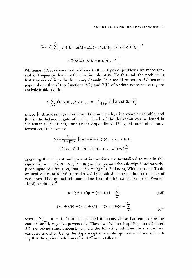
u2=-E,C [ Y~A(I~)-o(z~)+~(z~)-pz~~(z~)~,+,}~+s{o(z,)~,+,)’ ( = 0
Whiteman (1985) shows that solutions to these types of problems are more gen-
eral in frequency domains than in time domains. To this end, the problem is
first transferred into the frequency domain. It is useful to note as Whiteman’s
paper shows that if two functions A(L) and B(L) of a white noise process Ed are
analytic inside a disk:
where 6 denotes integration around the unit circle, z is a complex variable, and
l3z-l is the beta-conjugate of Z. The details of the derivation can be found in
Whiteman (1983, 1985), Taub (1990, Appendix A). Using this method of trans-
formation, U2 becomes:
u2=-&& b{Y(A-(o-r~))(A*-((J*-ran*))
+ soa* + G(A -(CT- p))(A* - (CT, - p*))$ $
assuming that all past and present innovations are normalized to zero.In this
equation r = 1 - pz, D = D(z), n = n(z) and so on, and the subscript * indicates the
B conjugate of a function, that is, D* = D(~z~‘). Following Whiteman and Taub,
optimal values of o and n are derived by employing the method of calculus of
variations. The optimal solutions follow from the following first order (Weiner-
Hopf) conditions:4
o-(yr+G)u=(y+G)A- i (3.6) -ml
(y-q + G)o - (yrr:v + G)/_t = (y* + GV - i &.,2 (3.7)
where, C-’ (Z = 1, 2) are unspecified functions whose Laurent expansions
contain stri?tly negative powers of Z. These two Weiner-Hopf Equations 3.6 and
3.7 are solved simultaneously to yield the following solutions for the decision
variables l.t and o. Using the Superscript to denote optimal solutions and not-
ing that the optimal solutions u* and o* are as follows:

8 QUARTERLY REVIEW OF ECONOMICS AND FINANCE
CC* = (ym:i: + G) - (y r + G) (yr* + G), (3.8)
p* = C-‘[C,’ {-6(y~e + G)}A] + (3.9)
o* = (y + G)A + (yr + G)C-'[C;;'{-6(yre + G)M]+ (3.10)
where the subscript + denotes the annihilator operator. The purely idiosyn- cratic nature of the shock introduces the possibility of complete insurance in this economy because individuals who experience positive (adverse) shocks attempt to smooth their consumption paths by purchasing additional goods with real balances from individuals who experience negative shocks. Money in this sense provides insurance to the individuals in this economy. Since the shock completely washes out at the aggregate level, the changes in individuals’ money demand and labor supply that occur in response to the shock do not affect the economy wide resource constraints.
Solution of the Problem for the Aggregate Shock
To determine an individual’s response to the random aggregate shock, the following portion of the Objective Function 3.2 is maximized:
U3+&${ ( - y w rn+H-D)(o*-r*x*+H*-D*)+&!m*
Using exactly the same techniques as before, the following Weiner-Hopf equa- tions are obtained:
w-G(l-r)n=(y+G)D- $ (3.11) -m3
(yr.+G)w-G(l-r.)rc=(yrr+G& (3.12) --4
In the Weiner-Hopf equations the Economy Wide Resource Constraint 2.6 has been substituted. When only the aggregate shock exists, Equation 2.6 becomes:
that is, H = TX. Using this and assuming that parameter values are such that
‘9 > $!, the following optimal values for w and n are obtained:
A STOCHOSTIC PRODUCTION ECONOMY 9
Z:,D
w4 = yp G+ypz, + i 1
-I
xc;’ = &{w*-(y+C)D}
(3.13)
(3.14)
To analyze these solutions, some structure is given to the driving process. If an autoregressive process of the following form is assumed:
where d is the parameter of autoregression, w* becomes:
using Lemma C.3 in Taub (1986). Since the shock ut has mean zero, on the average there is no shock to production. Consequently, there is no labor response to the shock on the average. However, the shock has positive variance which causes a variance in the labor supply function. Since the coefftcient y ppdl (6+y ppd) is less than 1, the variance of labor supply is less than the variance of the shock. Further, the variance of labor supply is positively related to money’s return, p. Unlike the idiosyncratic shock discussed above, the aggre- gate shock is uninsurable by mutual exchanges. Since individuals in this economy prefer smooth consumption paths but face such variable income paths, labor supply varies with the shock to ensure smooth consumption paths. The optimal solution shows that increases in money’s return provide greater incentives to produce and provide greater consumption smoothing by increas- ing the variability of the labor supply path. Since the coefhcient of the shock is less than one, perfect smoothing is not achieved.
While the section Solution of the Problem for the Deterministic Part of this paper and Kimbrough (1986) show that higher returns on money stimulate labor sup- ply in deterministic economies, this section has shown that higher returns on money also increase the variance of labor supply when income paths are subject to uninsurable stochastic shocks. It remains to be seen how optimal monetary policy responds to this type of response of labor supply to money. The issue of optimal monetary policy is discussed next.
IV. THE OPTIMUM QUANTITY OF MONEY
Operating in competitive markets, individuals take money’s rate of return as a market determined parameter in solving their optimization problems. This
10 QUARTERLY REVIEW OF ECONOMICS AND FINANCE
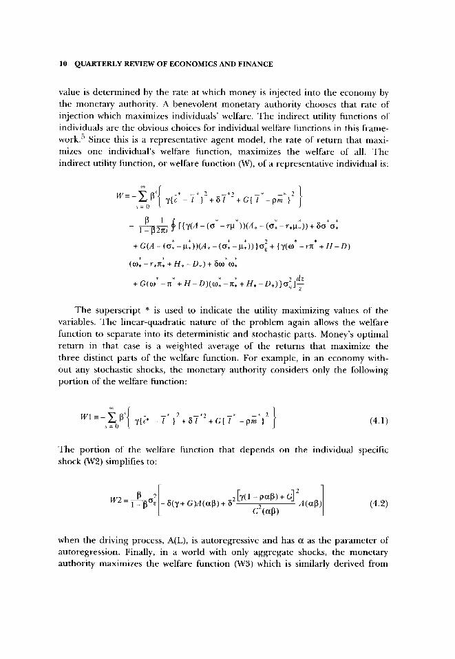
value is determined by the rate at which money is injected into the economy by the monetary authority. A benevolent monetary authority chooses that rate of injection which maximizes individuals’ welfare. The indirect utility functions of individuals are the obvious choices for individual welfare functions in this frame- work.’ Since this is a representative agent model, the rate of return that maxi- mizes one individual’s welfare function, maximizes the welfare of all. The indirect utility function, or welfare function (W), of a representative individual is:
WI-& yIt*_I*~2+*1*2+G(l*_pm~)2
\=O 1 1
- &A 4 [{y(A -(o* -rp*))(A* - (0: --r*pLr)) + &s*o:
+G(A-(o:-CI:))(A*-(o:-y:))}0,2+ {y(w*-rn*+H-D)
(ON: - r,x: + H, -D,) + &o*o:
The superscript * is used to indicate the utility maximizing values of the variables. The linear-quadratic nature of the problem again allows the welfare function to separate into its deterministic and stochastic parts. Money’s optimal return in that case is a weighted average of the returns that maximize the three distinct parts of the welfare function. For example, in an economy with- out any stochastic shocks, the monetary authority considers only the following portion of the welfare function:
WI=-CP‘ y{c* _y>2+8C*2+G(y +m’j2 - i \ = 0 1 (4.1)
The portion of the welfare function that depends on the individual specific shock (W2) simplifies to:
*[IY(l -wlu+G12 C2(uP)
(4.2)
when the driving process, A(L), is autoregressive and has cx as the parameter of autoregression. Finally, in a world with only aggregate shocks, the monetary authority maximizes the welfare function (W3) which is similarly derived from
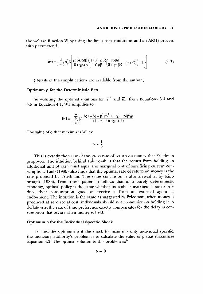
A STOCHOSTIC PRODUCTION ECONOMY 11
the welfare function W by using the first order conditions and an AR(l) process with parameter d.
(4.3)
(Details of the simplifications are available from the author.)
Optimum p for the Deterministic Part
Substituting the optimal solutions for 7 * and ii7 from Equations 3.4 and 3.5 in Equation 4.1, Wl simplifies to:
Wls-2 p’ 6( 1 - 6) + P2YP2( 1-Y) - 2WYP
\=O (1-r-WPYP+S)
The value of p that maximizes Wl is:
This is exactly the value of the gross rate of return on money that Friedman proposed. The intuition behind this result is that the return from holding an additional unit of cash must equal the marginal cost of sacrificing current con- sumption. Taub (1989) also finds that the optimal rate of return on money is the rate proposed by Friedman. The same conclusion is also arrived at by Kim- brough (1986). From these papers it follows that in a purely deterministic economy, optimal policy is the same whether individuals use their labor to pro- duce their consumption good or receive it from an external agent as endowment. The intuition is the same as suggested by Friedman; when money is produced at zero social cost, individuals should not economize on holding it. A deflation at the rate of time preference exactly compensates for the delay in con- sumption that occurs when money is held.
Optimum p for the Individual Specific Shock
To find the optimum p if the shock to income is only individual specific, the monetary authority’s problem is to calculate the value of p that maximizes Equation 4.2. The optimal solution to this problem is:6
p=o
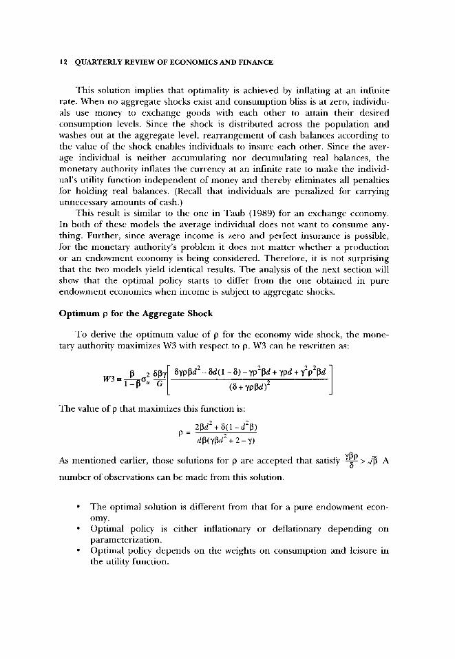
12 QUARTERLY REVIEW OF ECONOMICS AND FINANCE
This solution implies that optimality is achieved by inflating at an infinite rate. When no aggregate shocks exist and consumption bliss is at zero, individu- als use money to exchange goods with each other to attain their desired consumption levels. Since the shock is distributed across the population and washes out at the aggregate level, rearrangement of cash balances according to the value of the shock enables individuals to insure each other. Since the aver- age individual is neither accumulating nor decumulating real balances, the monetary authority inflates the currency at an infinite rate to make the individ- ual’s utility function independent of money and thereby eliminates all penalties for holding real balances. (Recall that individuals are penalized for carrying unnecessary amounts of cash.)
This result is similar to the one in Taub (1989) for an exchange economy. In both of these models the average individual does not want to consume any- thing. Further, since average income is zero and perfect insurance is possible, for the monetary authority’s problem it does not matter whether a production or an endowment economy is being considered. Therefore, it is not surprising that the two models yield identical results. The analysis of the next section will show that the optimal policy starts to differ from the one obtained in pure endowment economies when income is subject to aggregate shocks.
Optimum p for the Aggregate Shock
To derive the optimum value of p for the economy wide shock, the mone- tary authority maximizes W3 with respect to p. W3 can be rewritten as:
6yppd2-6d(l-6)-yp2pd+ypd+y2p2pd
(6 + rpPd)2 1 The value of p that maximizes this function is:
p = 2f3d2 + 6( 1 -d2p)
dP(@d2 + 2 -Y)
As mentioned earlier, those solutions for p are accepted that satisfy ‘+ > ,& A
number of observations can be made from this solution.
l The optimal solution is different from that for a pure endowment econ- omy.
l Optimal policy is either inflationary or deflationary depending on parameterization.
l Optimal policy depends on the weights on consumption and leisure in the utility function.
A STOCHOSTIC PRODUCTION ECONOMY 13
Optimal policy is different for this production economy from that for a pure endowment economy considered in Taub (1989) because individuals in this production economy respond to the shock by changing labor supply. As seen in the section, Solutions of the Problem for the Aggregate Shock, changes in money’s return change the variance of the labor supply function. Money in that event influences the consumption smoothing effect individuals attempt to achieve by changing labor supply in response to the aggregate shock. The resulting optimal policy therefore depends on this additional feature of individ- uals’ behaviors.
The complexity of optimal monetary policy and its sensitivity to the two fac- tors mentioned above is also apparent from the nature of the solution. Examination of the optimal solution indicates that optimal policy may be either inflationary or deflationary depending on the parameterization. Deflation is optimal when the numerator exceeds the denominator. That is, when
dp 6>- (l-d P)
(31 -d)-y(1 -d*p))
Inflation is optimal otherwise. Some additional insights into the nature of the policy can be gained by
examining how it responds to changes in some of the parameters. For example,
ap l-d*P >. x = dP(yPd* + 2 - y)
Since the numerator is always positive, the optimal rate of return on money increases as the weight individuals ascribe to the disutility from work increases. Since a higher 6 reduces the incentive to work and thereby inhibits individuals from attaining a smooth intertemporal consumption path, money’s return is increased to compensate for the decline in the variance of the labor supply function.
The dependence of optimal policy on the weight individuals give to the util- ity they derive from consumption is given by:
ap (1 - d2p)(2pd2 + 6( 1 - d*p)) ;ry=
dP(rPd* + 2 - r)*
This is again positive and the intuition is straightforward. The more indi- viduals value consumption, ceteris paribus, the greater is the incentive to produce and reach the consumption target. The positive relationship between p and the variance of labor supply explains this relationship between p and y.
14 QUARTERLY REVIEW OF ECONOMICS AND FINANCE
V. CONCLUSION
In the context of an economy in which individuals produce a consumption good by supplying their labor services and production functions are buffeted by sto- chastic shocks each period, this paper has (1) analyzed how individuals’ labor- leisure decisions depend on money’s rate of return and (2) determined the rate of return that maximizes welfare. In this economy, where cash-in-advance is required for all transactions and money is the only asset, money plays a signifi- cant role in both consumption-savings and labor-leisure decisions of house- holds. Since individuals cannot consume their own production and past balances are necessary for current consumption, the inflation tax plays a major role in their labor supply decision. It is found that an increase in money’s return reduces the tax on labor income and stimulates labor supply and production when no uncertainties exist. This result is similar to what Kimbrough (1986) found in the context of a deterministic economy in which increases in money’s return increase the quantity of money held and release time from shopping. In contrast to Kimbrough’s paper this paper considered stochastic disturbances to the income process. It is found that if an aggregate shock that has mean zero but positive variance affects production, labor supply closely follows the random disturbance. Such a relationship between the shock and labor supply exists here because it helps smooth the consumption path. Increases in money’s return are found to improve this consumption smoothing process by increasing the vari- ance of labor supply.
In an economy where money affects both the deterministic component and variance of labor supply, optimal monetary policy is more complex than what Friedman’s proposition suggests. In deriving money’s optimal return (or the optimal inflation tax), the paper finds that if no uncertainties exist, Friedman’s proposition of deflation at the economy’s rate of time preference remains opti- mal. If uncertainties exist, however, Friedman’s rule is no longer optimal. In particular, in the face of purely idiosyncratic shocks, since exchanges between individuals can eliminate the shock and provide complete insurance, optimal policy is highly inflationary. In contrast, when aggregate uncertainty exists the shock is uninsurable by mutual exchanges and individuals attempt to insure themselves by adjusting their labor supply path. This insurance against the vari- ability of the shock by labor plays a significant role in money’s optimal return. The policy is found to depend on the various parameters of the model and is either inflationary or deflationary. Since disposal is expensive, optimal policy is such that it balances the positive effects of low inflation taxes on labor supply and the negative effects of excessive cash holdings that low taxes encourage. This result significantly differs from the optimal policy derived by Taub for a very similar but pure endowment economy.
Acknowledgment: This paper is a part of my dissertation submitted to the faculty of the
Virginia Polytechnic Institute and State University. I thank Richard Cothren and all other
A STOCHOSTIC PRODUCTION ECONOMY 15
committee members for their very helpful comments and suggestions. I also thank Bart Taub for introducing me to the Weiner-Hopf technique used in this paper and an anony- mous referee for very useful suggestions. The usual disclaimer applies.
NOTES
*Direct all correspondence to: Nivedita Mukherji, Oakland University, School of Business dministration, Rochester, MI 48309-4401.
1. The terms individuals and households will be used synonymously when the dis- tinction between a shopper and a worker is not important.
2. These motivations for the cash-in-advance restriction is similar to those found in Lucas-Stokey (1987), Townsend (1980), Chari et al. (1993).
3. See Taub (1989) for a similar penalty function mimicking cash-in-advance restrictions.
4. Details of the derivation are available from the author upon request. 5. Other types of welfare functions are, however, clearly possible. 6. The proof is available from the author upon request.
REFERENCES
Bewley, Truman. 1983. “A Difficulty with the Optimum Quantity of Money,” Econometrica, 51: 1485-1504 .
Chari, V.V., L.J. Christiano, P.J. Kehoe. 1993. “Optimality of the Friedman Rule in Economies with Distorting Taxes.” Federal Reserve Bank of Minneapolis Stuff Report 158.
Friedman, Milton. 1969. “The Optimum Quantity of Money.” Pp. l-50 in The Optimum
Quantity of Money and Other Essays. Chicago: Aldine. Kimbrough, Kent. 1986. “Inflation, Employment, and Welfare in the Presence of
Transactions Costs,” Journal of Mon,ey, Credit, LY Banking, 18: 127- 140.
Lucas, R.E. and N.L. Stokey. 1987. “Money and Interest in a Cash-in-Advance Economy.” Econometrica, 55: 49 l-5 14.
Mukherji, Nivedita. 1992. “The Optimum Quantity of Money in a Stochastic Economy: A Comment.” International Economic Review, 33: 487-489.
Taub, Bart. 1986. “The Tradeoff Between Social Insurance and Aggregate Fluctuations.” Infbrmation Economics and Policy, 2: 259-276.
. 1989. “The Optimum Quantity of Money in a Stochastic Economy,” Znternational
Economic Review, 30: 255-273.
-. 1990. “The Equivalence of Lending Equilibria and Signaling-Based Insurance Under Asymmetric Information,” KAND Journal of Economics, (Autumn).
Townsend, Robert. 1980. “Models of Money with Spatially Separated Agents.” Pp. 265. 303 in Federal Reserve Bank of Minneapolis, Models ofMonetq Economics, edited by J.M. Karaken and N. Wallace.
Whiteman, Charles. 1983. Linear Ration,al Expectations Models: A User’s Guide. University of Minnesota Press.

16 QUARTERLY REVIEW OF ECONOMICS AND FINANCE
-. 1985. “Spectral Utility, Weiner-Hopf Techniques, and Rational Expectations,” Journal of Economic Dynamics and Control, 9: 225-240.
Woodford, Michael. 1990. “The Optimum Quantity of Money.” Pp. 1067-l 152 in Handbook of MonetaT Economics, Vol. 11, edited by Benjamin Friedman and Frank Hahn. Amsterdam: North-Holland.