A profiler for a heterogeneous multi-core multi-FPGA system
61
A Profiler for a Heterogeneous Multi-Core Multi-FPGA System by Daniel Pereira Nunes A thesis submitted in conformity with the requirements for the degree of Master of Applied Sciences Graduate Department of Electrical and Computer Engineering University of Toronto Copyright c 2008 by Daniel Pereira Nunes
-
Upload
independent -
Category
Documents
-
view
0 -
download
0
Transcript of A profiler for a heterogeneous multi-core multi-FPGA system
A Profiler for a Heterogeneous Multi-Core Multi-FPGA System
by
Daniel Pereira Nunes
A thesis submitted in conformity with the requirementsfor the degree of Master of Applied Sciences
Graduate Department of Electrical and Computer EngineeringUniversity of Toronto
Copyright c© 2008 by Daniel Pereira Nunes
A Profiler for a Heterogeneous Multi-Core Multi-FPGA System
Daniel Pereira NunesMaster of Applied Sciences
Graduate Department of Electrical and Computer EngineeringUniversity of Toronto
2008
Abstract
The TMD is a heterogeneous multi-FPGA system that uses the Message Passing Interface
(MPI) programming model to build systems comprised of processors and hardware engines
implemented on FPGAs, all interacting using MPI messages. This thesis implements a profil-
ing system that can monitor communication calls and user states. The data is compatible with
Jumpshot, a visualizer already used for software-based MPIapplications. We demonstrate the
capability of the profiler on a number of applications and show that the profiler can be used for
multiple FPGAs across multiple boards.
ii
Acknowledgements
First and foremost I would like to thank my supervisor Professor Paul Chow for his guidanceand technical advice which were of highest value throughoutthe course of this MASc. I wouldalso like to thank Emanuel and Alex, for their suggestions and conversations; Manuel, Arunand Chris for their expertise advice; and all the remaining group members: Andrew, Danny,David, Ali, Keith, Daniel Ly, Danyao, Richard, Tom, Mike, Nasim, and Matt for their support.Last but not the least, Professor Joao Cardoso who first contacted the University of Torontoand provided guidance throughout all my undergrad in Portugal.
iii

Contents
1 Introduction 1
1.1 Motivation . . . . . . . . . . . . . . . . . . . . . . . . . . . . . . . . . . . . . 1
1.2 Research Contributions . . . . . . . . . . . . . . . . . . . . . . . . . . . . .. 2
1.3 Thesis Organization . . . . . . . . . . . . . . . . . . . . . . . . . . . . . .. . 3
2 Background 4
2.1 MPI . . . . . . . . . . . . . . . . . . . . . . . . . . . . . . . . . . . . . . . . 4
2.2 The TMD . . . . . . . . . . . . . . . . . . . . . . . . . . . . . . . . . . . . . 5
2.2.1 Computation nodes . . . . . . . . . . . . . . . . . . . . . . . . . . . . 7
2.2.2 Off-Chip Communications Nodes . . . . . . . . . . . . . . . . . . . . 7
2.3 BEE2 . . . . . . . . . . . . . . . . . . . . . . . . . . . . . . . . . . . . . . . 8
2.4 Performance Analysis for Reconfigurable Computers . . . . . .. . . . . . . . 8
2.5 Related Work . . . . . . . . . . . . . . . . . . . . . . . . . . . . . . . . . . . 10
3 Profiler 12
3.1 Hardware . . . . . . . . . . . . . . . . . . . . . . . . . . . . . . . . . . . . . 12
3.2 Clock Counter Synchronization . . . . . . . . . . . . . . . . . . . . . . .. . . 15
3.3 Software . . . . . . . . . . . . . . . . . . . . . . . . . . . . . . . . . . . . . . 17
4 Case Studies 19
4.1 Barrier . . . . . . . . . . . . . . . . . . . . . . . . . . . . . . . . . . . . . . . 19
4.2 The Heat Equation Application . . . . . . . . . . . . . . . . . . . . . .. . . . 22
4.3 The LINPACK Benchmark . . . . . . . . . . . . . . . . . . . . . . . . . . . . 26
4.4 TMD-MPE - Unexpected Messages Queue . . . . . . . . . . . . . . . . .. . 32
5 Profiler Overhead 35
6 Profiler Implementation on Other Platforms 37
6.1 Backplane . . . . . . . . . . . . . . . . . . . . . . . . . . . . . . . . . . . . . 37
iv

6.2 HPRC Implementation Platform . . . . . . . . . . . . . . . . . . . . . . .. . 39
7 Conclusions 41
8 Future Work 43
9 Appendixes 45
9.1 Appendix A . . . . . . . . . . . . . . . . . . . . . . . . . . . . . . . . . . . . 45
9.1.1 Example System . . . . . . . . . . . . . . . . . . . . . . . . . . . . . 45
9.1.2 Tracer . . . . . . . . . . . . . . . . . . . . . . . . . . . . . . . . . . . 47
9.1.3 Gather . . . . . . . . . . . . . . . . . . . . . . . . . . . . . . . . . . . 48
9.1.4 Collector . . . . . . . . . . . . . . . . . . . . . . . . . . . . . . . . . 49
Bibliography 51
v
List of Tables
4.1 State’s Duration . . . . . . . . . . . . . . . . . . . . . . . . . . . . . . . . .. 29
5.1 Tracers Overhead . . . . . . . . . . . . . . . . . . . . . . . . . . . . . . . . .36
9.1 MPETracer’s Interface . . . . . . . . . . . . . . . . . . . . . . . . . . . . . . 47
9.2 Gather Interface . . . . . . . . . . . . . . . . . . . . . . . . . . . . . . . . .. 48
9.3 Collector Interface . . . . . . . . . . . . . . . . . . . . . . . . . . . . . . .. 49
vi
List of Figures
2.1 TMD Architecture . . . . . . . . . . . . . . . . . . . . . . . . . . . . . . . . 6
2.2 BEE2 Architecture . . . . . . . . . . . . . . . . . . . . . . . . . . . . . . . . 8
3.1 High-Level Profiler Architecture . . . . . . . . . . . . . . . . . . .. . . . . . 13
3.2 a) Processor Profiler Architecture b) Hardware Engine Profiler Architecture . . 14
3.3 a) Communication Tracer b) Computation Tracer (Processor) c) Computation
Tracer (Engine) . . . . . . . . . . . . . . . . . . . . . . . . . . . . . . . . . . 16
4.1 Barrier Communication Patterns . . . . . . . . . . . . . . . . . . . . . .. . . 20
4.2 Barrier implemented sequentially . . . . . . . . . . . . . . . . . . .. . . . . . 21
4.3 Barrier implemented as a binary tree . . . . . . . . . . . . . . . . . .. . . . . 21
4.4 Data decomposition and point-to-point communication in Jacobi algorithm . . 23
4.5 Using blocking calls . . . . . . . . . . . . . . . . . . . . . . . . . . . . . .. 25
4.6 Using non-blocking calls . . . . . . . . . . . . . . . . . . . . . . . . . .. . . 25
4.7 Linpack Benchmark Testbed . . . . . . . . . . . . . . . . . . . . . . . . . .. 28
4.8 Linpack Benchmark Iteration . . . . . . . . . . . . . . . . . . . . . . . .. . . 30
4.9 Linpack Benchmark General View . . . . . . . . . . . . . . . . . . . . . .. . 31
4.10 Barrier implemented sequential with TMD-MPE profiled . .. . . . . . . . . . 33
6.1 The Backplane . . . . . . . . . . . . . . . . . . . . . . . . . . . . . . . . . . 38
6.2 Possible Implementation of the Profiler on the Backplane .. . . . . . . . . . . 39
6.3 Possible Implementation of the Profiler on the HPRC Platform . . . . . . . . . 40
9.1 Example system . . . . . . . . . . . . . . . . . . . . . . . . . . . . . . . . . . 46
vii
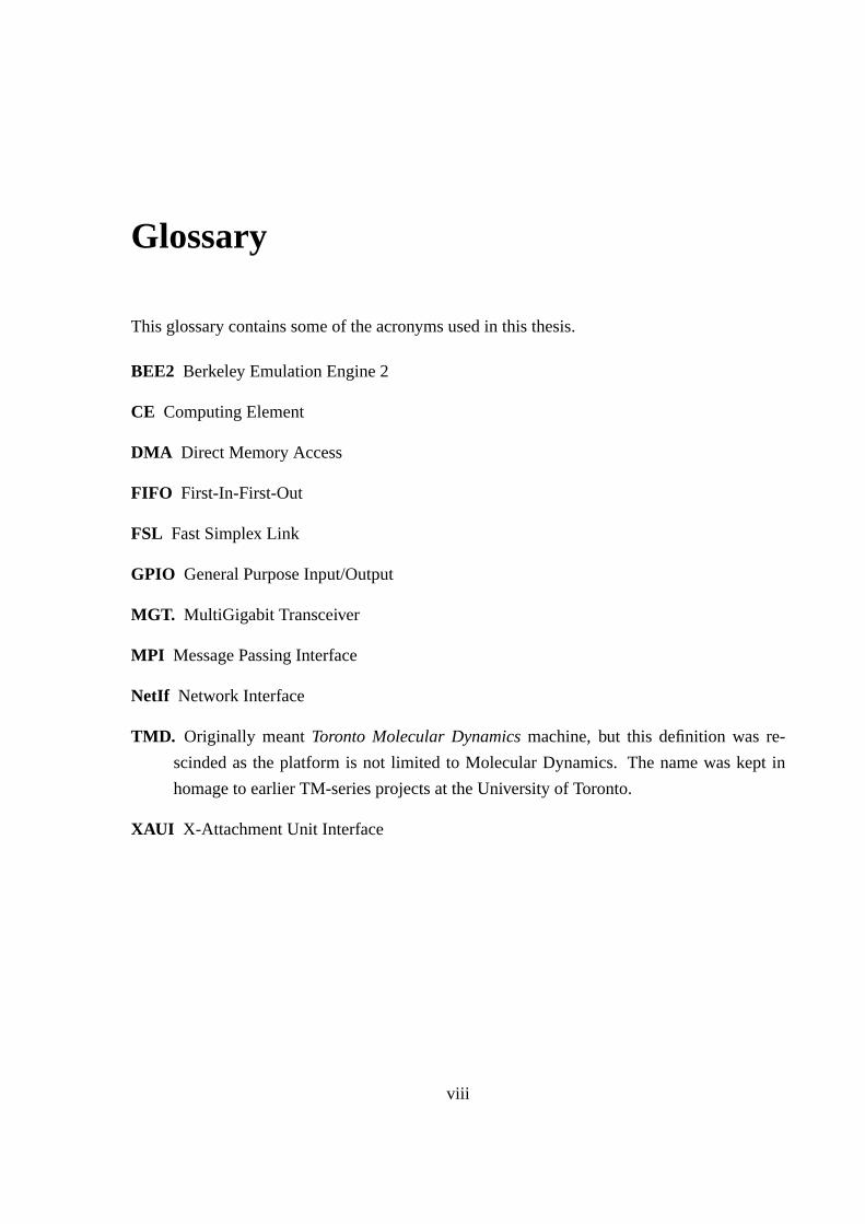
Glossary
This glossary contains some of the acronyms used in this thesis.
BEE2 Berkeley Emulation Engine 2
CE Computing Element
DMA Direct Memory Access
FIFO First-In-First-Out
FSL Fast Simplex Link
GPIO General Purpose Input/Output
MGT. MultiGigabit Transceiver
MPI Message Passing Interface
NetIf Network Interface
TMD. Originally meantToronto Molecular Dynamicsmachine, but this definition was re-
scinded as the platform is not limited to Molecular Dynamics. The name was kept in
homage to earlier TM-series projects at the University of Toronto.
XAUI X-Attachment Unit Interface
viii
Chapter 1
Introduction
This chapter provides details of the motivation of this thesis in Section 1.1. Section 1.2 outlines
the main contributions of this work, and Section 1.3 presents a summary of the content of the
remaining chapters of this thesis.
1.1 Motivation
Understanding the behavior of computer applications without the aid of program analysis tools
can become a tedious, and sometimes impossible, task. Computer applications range from sim-
ple sequential codes, where an analysis of the current position within the source code may be
sufficient to understand it, to complicated parallel codes running on heterogeneous systems that
require not only the position of each processor within its source code but also a time relation-
ship between them. A profiler goal is to give understanding ofthe application while requiring
the smallest effort from the programmer and without affecting the system significantly.
Field-Programmable Gate Array (FPGA) reconfigurability allows us to gain performance
by creating application-specific hardware. Some high-performance computing platforms now
include FPGAs that can be plugged directly into an Intel Front Side Bus (FSB) [1] socket or
an AMD Opteron [2] socket using the hyper-transport protocol. Some systems rely only on
FPGAs, taking advantage of their embedded cores (e.g. PowerPC [3]) for general computation
1

CHAPTER 1. INTRODUCTION 2
and specialized hardware engines for the more demanding computation. However, failing to
have a complete understanding of the application may resultin underachieved performance.
To address this, FPGA reconfigurability may also be used to create a custom profiler that will
provide the knowledge needed to configure the hardware system for a specific application.
This thesis focus is a profiler for the TMD [4] [5] [6], a heterogeneous multi-core multi-
FPGA system designed at the University of Toronto that uses the message passing paradigm
for communications. The main purpose of this profiler is to give insight into the communica-
tions occurring between nodes and the computation performed by each node. The presence of
different cores in the system increases the difficulty of profiling, since the profiler is required
to be compatible with all of them. Furthermore, the possibility of having hardware engines
introduces the need of having the profiler’s functionality implemented both in software and
hardware.
1.2 Research Contributions
The contributions of this thesis are derived from the integration of ideas already used in other
systems (e.g. traditional clusters) into a new multi-core multi-FPGA system, the TMD. Due to
the different nature of traditional clusters and the TMD, the implementation of such ideas differ
completely “under the hood”, but provide the opportunity for users to profile their applications
using interfaces already familiar to them. Following the same easy-to-port philosophy of the
TMD, users are able to port their already instrumented source code from a cluster into the TMD
in a seamless way.
The profiler infrastructure provides a first attempt of profiling these systems and can be
used as a working platform for future students at the University of Toronto that wish to research
further into performance analysis.
CHAPTER 1. INTRODUCTION 3
1.3 Thesis Organization
The remainder of this thesis is organized as follows: Chapter2 provides background informa-
tion to better understand the contents of this thesis. Chapter 3 describes the profiler implemen-
tation. In Chapter 4 the profiler is tested with four case studies. Then in Chapter 5 the profiler
overhead is considered. Chapter 6 considers the implementation of the profiler on other imple-
mentations of the TMD. Finally, Chapter 7 concludes and in Chapter 8 ideas are presented for
future work.
In the appendix there is helpful information on how to include the profiler on a hardware
system.
Chapter 2
Background
This chapter presents a brief overview of key concepts to better understand this work, and to
establish a context for the ideas presented in this thesis. Each section describes parts of related
knowledge and presents some definitions that will be used in the rest of this document. Sec-
tion 2.1 is a brief introduction to the known message passinglibrary, MPI [7] [8]. Section 2.2
and Section 2.3 describe the hardware system on which the profiler was applied. Section 2.4
introduces the challenges of performance analysis for reconfigurable computers. Section 2.5
examines related work in the field of profiling, both in sequential and parallel applications, and
traditional clusters and FPGA systems.
2.1 MPI
Message passing has become a common programming model used for distributed memory
computing systems. Message passing assumes that each process contains the necessary data
in local memory and that no direct access to global memory is available. Transactions be-
tween processes are defined explicitly by the programmer, which is also responsible for the
execution’s correctness. MPI, the best known message passing library, provides a language
and architecture independent communication protocol thatis highly scalable and portable. It
was created in 1992 and is currently maintained by the MPI Forum [7]. The API is organized
4

CHAPTER 2. BACKGROUND 5
in layers built on top of each other. While the lower layers arehardware dependent and need to
be adapted for different architectures, the upper layers are standard and allow the user code to
be usable across different platforms. This portability is one of the main reasons for the success
of MPI. Communications can be done by point-to-point or collectively calls. Point-to-point
calls,MPI SendandMPI Recv, are use to send and receive data, respectively. Collective calls
are built on top of point-to-point calls simplifying the user code by defining important group
communication. Examples of collective calls areMPI Barrier, a synchronization routine, and
MPI Broadcast, a routine where one process broadcasts data to all the others.
The communication protocol can be either synchronous or asynchronous. TheRendezvous
protocol is a synchronous communication mode where a process will only initiate a trans-
fer when the receiver acknowledges the operation. The transfer is initiated by the producer
process sending arequest to sendpacket composed of its rank, a destination rank, size of mes-
sage and a 32-bit tag, which is a user-defined message identificator. TheEagerprotocol is an
asynchronous protocol communication mode where a process will initiate a transfer without
consulting the other process. In this communication mode, the producing process assumes that
enough buffering exists to hold its message at the receiver.
Each process is represented by a unique integer, called the rank, spanning from 0 to size-1,
where size is the total number of processes on the system.
2.2 The TMD
The TMD is a heterogeneous multi-core, multi-FPGA system developed at the University of
TMD that achieves high performance by taking advantage of hardware acceleration using FP-
GAs. The system can be fully customized to a specific application by adapting the on-chip
network topology and choosing appropriate computation elements for each task. The possi-
bility of having heterogeneous cores requires a flexible communication protocol that is not
dependent on any particular computation element, and that simultaneously allows the seamless
CHAPTER 2. BACKGROUND 6
addition, removal or exchange of cores to better fit a particular application. This flexibility
co-exists in this system both in the hardware level, where a node can be physically removed
without changing the rest of the system, and in the software level where the source code of an
application is independent of the number and nature of nodes.
PPC
MPE
PPC
MPE
MPE
InterChip
FSL XAUI
InterChip
FSL XAXX UI
MPE
PPPPCC
MMPPEE
Computation Node
Computation Node
Off-Chip Communications Node
Network
Interface
Network
InterfaceHardware Engine
Network
On-chip
Network
On-chip
FSL
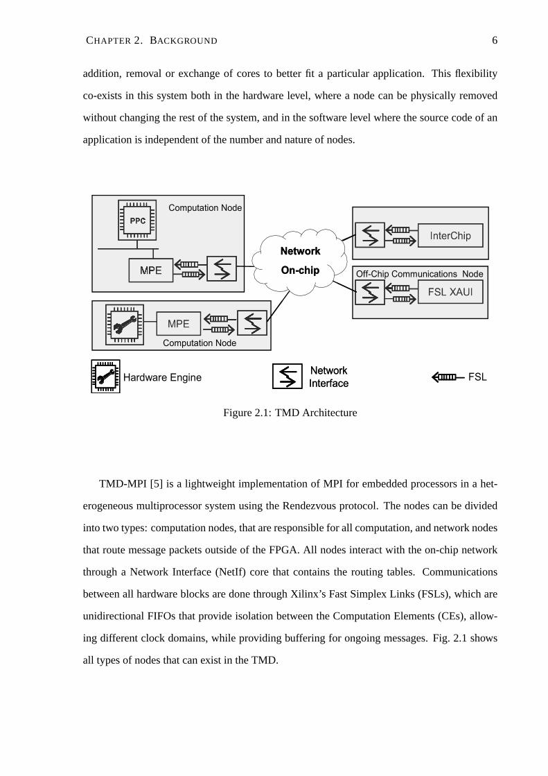
Figure 2.1: TMD Architecture
TMD-MPI [5] is a lightweight implementation of MPI for embedded processors in a het-
erogeneous multiprocessor system using the Rendezvous protocol. The nodes can be divided
into two types: computation nodes, that are responsible forall computation, and network nodes
that route message packets outside of the FPGA. All nodes interact with the on-chip network
through a Network Interface (NetIf) core that contains the routing tables. Communications
between all hardware blocks are done through Xilinx’s Fast Simplex Links (FSLs), which are
unidirectional FIFOs that provide isolation between the Computation Elements (CEs), allow-
ing different clock domains, while providing buffering forongoing messages. Fig. 2.1 shows
all types of nodes that can exist in the TMD.
CHAPTER 2. BACKGROUND 7
2.2.1 Computation nodes
Computation can be performed by a Microblaze, a PowerPC or a hardware engine. Because the
application source code can be kept constant from platform to platform, due to the TMD-MPI
abstraction, a Microblaze or a PowerPC can be used as an intermediate stage when porting an
application from a traditional cluster to the TMD. After theapplication is successfully ported
in software, if the task running on one of these processors iscritical it may then be optimized
by substituting it with a hardware engine. Because all communications are done using the
TMD-MPI protocol, a special core that encapsulates the TMD-MPI functionality, the TMD-
Message Passing Engine (TMD-MPE) [6], was designed so all hardware engines can send and
receive messages from other nodes in full-duplex mode. Thissimplifies significantly the design
process of a hardware engine, as the designer will not need tobe concerned with the details
of the protocol such as unexpected messages and packetization. Although the TMD-MPE
was mainly designed to be used by engines, it can also be used by a Microblaze or a PowerPC,
reducing the memory footprint of their code and, for the processors, increasing communication
speed by allowing Direct Memory Access (DMA).
2.2.2 Off-Chip Communications Nodes
Off-chip communications nodes do not perform any computation and are present on the system
to route message packets outside to another FPGA. Their configuration depends on which plat-
form the TMD is being implemented on. This paper will only consider the Berkeley Emulation
Engine 2 (BEE2) [9] boards for implementation (see Section 2.3 ). There are two possible types
of off-chip communications on the BEE2 board implementation: intra-board and inter-board.
The intra-board communications refer to messages sent between nodes from different FPGAs
on the same board and are done using direct connection wires between the FPGAs, through
the Interchip core. The inter-board communications refer to communications performed by
different nodes in different boards and are done using the X Attachment Unit Interface (XAUI)
standard. As with all blocks, the interface between the on-chip network and XAUI is done
CHAPTER 2. BACKGROUND 8
using the FSL standard.
2.3 BEE2
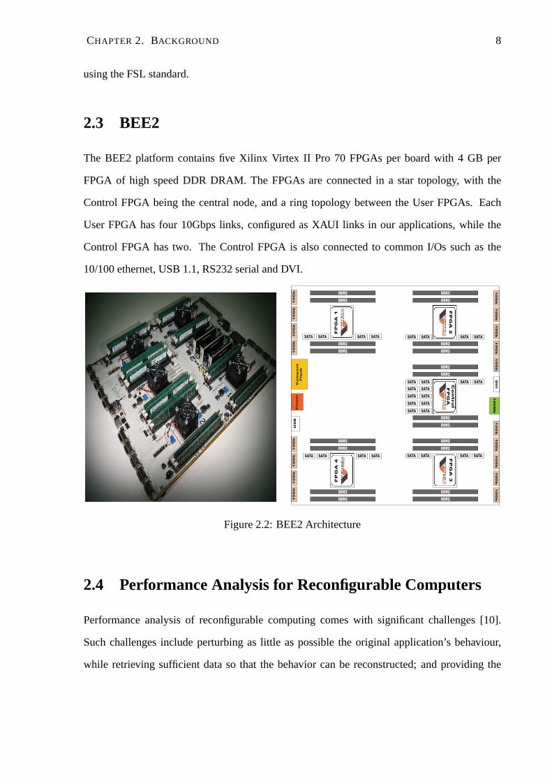
The BEE2 platform contains five Xilinx Virtex II Pro 70 FPGAs per board with 4 GB per
FPGA of high speed DDR DRAM. The FPGAs are connected in a star topology, with the
Control FPGA being the central node, and a ring topology between the User FPGAs. Each
User FPGA has four 10Gbps links, configured as XAUI links in our applications, while the
Control FPGA has two. The Control FPGA is also connected to common I/Os such as the
10/100 ethernet, USB 1.1, RS232 serial and DVI.
10
Gb
10
Gb
10
Gb
10
Gb
10
Gb
10
Gb
10
Gb
10
Gb
10
Gb
10
Gb
10
Gb
10
Gb
10
Gb
10
Gb
10
Gb
10
Gb
10
Gb
10
Gb
DDR2
DDR2
DDR2
DDR2
DDR2
DDR2
DDR2
DDR2
DDR2
DDR2
DDR2
DDR2
DDR2
DDR2
DDR2
DDR2
DDR2
DDR2
DDR2
DDR2
Co
ntro
l
FP
GA
FP
GA
2
FP
GA
3
FP
GA
1
FP
GA
4
10
0M
bD
VI
Pow
er
US
BC
om
pa
ct
Fla
sh
SATA SATASATA SATA
SATA SATASATA SATA SATA SATASATA SATA
SATA SATASATA SATA
SATA SATASATA SATA
SATA SATA
SATA SATA
SATA SATA
SATA SATA
Figure 2.2: BEE2 Architecture
2.4 Performance Analysis for Reconfigurable Computers
Performance analysis of reconfigurable computing comes with significant challenges [10].
Such challenges include perturbing as little as possible the original application’s behaviour,
while retrieving sufficient data so that the behavior can be reconstructed; and providing the

CHAPTER 2. BACKGROUND 9
flexibility to analyze different applications, while requiring little effort from the designer.
What data to instrument plays an important role in reconfigurable computers analysis. Pos-
sible causes of performance bottlenecks in hardware are notas well determined as they are in
software, and the immense number of hardware systems makes it harder to have a common
bottleneck guide. Nevertheless, communications, off-chip (e.g. FPGA, CPU, main memory),
on-board (e.g. FPGA, DDR) or on-chip (e.g. CE), are a known source of bottlenecks. However,
instrumenting all communications can become a challenge due to the amount of parallelism in-
side a FPGA. The TMD-MPI (see Section 2.2) in conjunction with the TMD-MPE and the
FIFO-based on-chip network, provides an excellent abstraction for the communications. This
abstraction allows not only running an application as it would be run in a traditional cluster,
but also to profile it as such. This is, the FPGA is not profiled as one uniform core, but as
multiple independent cores. Another important step prior to instrumentation is to decide at
what level that instrumentation should be performed. Instrumentation can be performed either
at a source-level or binary-level. Although other intermediate levels may exist, the fact that
some only exist in memory during synthesis and implementation, and their documentation is
poor, reduces the advantages of using them and are out of the scope of this work. Binary-level
instrumentation provides a fast method of performing changes on the application since it oc-
curs after place-and-route. Also, it’s portable across languages for a specific device. However,
instrumenting a bitstream is extremely hard. Not all data isaccessible, and correlation with the
source will be impossible most of the time since synthesis and implementation significantly
transform the system. Source-level instrumentation allows correlation with the source, it’s eas-
ier to implement and portable across devices. The largest setback is the number of hours it may
take to instrument since any change to the system at source-level requires the system to be built
again.

CHAPTER 2. BACKGROUND 10
2.5 Related Work
A large amount of research has been done to create or improve profilers. Profiling data can be
gathered from hardware performance counters, that collectlow level performance metrics (e.g.
clock cycles, instruction counts, cache misses) or from thesource code itself by instrumenting
it. In 1979, Unix systems included a tool calledprof that would list each function and give
the number of calls and time spent on them.Gprof [11] was released in 1982 and included a
call graph analysis that would provide not only the time spent in each function but also how
much time each function spent on behalf of each of its callers. The Performance Application
Programming Interface (PAPI) [12] gives access to hardwareperformance counters on modern
microprocessors allowing the monitoring of high-level hardware events.
For parallel systems, such as multicore processors, profilers that can relate events over
different processors and provide information on the interactions of different processing units
during a parallel application execution are needed.
Reconfigurable systems can be more challenging to profile thantypical clusters of comput-
ers. The profilers available tend to gather data from the perspective of a CPU. However, FPGA
systems may not have any conventional processor and will most certainly contain hardware en-
gines that will require a more hardware-aware profiler. Techniques like Xilinx ChipScope [13]
and Altera’s SignalTap [14] have been developed to extract data out of an FPGA with little
impact on performance. However, these tools were designed for hardware debugging and are
far from adequate to be used as profilers.
The Snooping Software Profiler (SnoopP) [15] is a non-intrusive, real time, profiling tool
developed at the University of Toronto. The profiler is able to count how many cycles an
application running on a soft-core processor spent in a specific program counter (PC) address
region.
The MPI Parallel Environment [16] provides the ability to profile different sections of MPI
code, including communications performed between nodes, through instrumentation of the
source code. However, it is an intrusive profiler that will add close to 5% overhead to a typ-
CHAPTER 2. BACKGROUND 11
ical application [17]. It includes a tool called JumpShot [16] that visualizes the profiler logs,
allowing a user to see what each process is doing over a commontimeline. The logs created
by the profiler presented in this paper are compatible with the logs created by the MPI Par-
allel Environment. Moreover, it uses the same Application Programming Interface (API) to
instrument the source code. This was done because the MPI Parallel Environment is part of
the MPI distribution MPICH [16] and will allow us to easily port profiled applications from a
traditional cluster to the TMD. Also, Jumpshot is an easy to use visualization tool that is able
to open considerably large profiler logs.

Chapter 3
Profiler
The reprogrammable nature of the FPGAs can be used in our favour to create a custom profiler
for an application that will minimally impact the system performance, therefore, retrieving the
real behavior of the system.
This profiler retrieves data from all TMD-MPI communicationcalls and computation states
defined by the user, both from a processor or a hardware engine, and allows the visualization of
all ranks on a timeline. Hardware is profiled by sampling specific hardware events. Software
is profiled by embedding code into the MPI functions or using additional profiling functions.
3.1 Hardware
The profiler hardware should occupy minimal FPGA real estateand not affect timing by mak-
ing the application run at a slower clock rate. Unfortunately, these are conflicting goals and a
compromise had to be made. We incurred extra hardware to prevent performance loss when-
ever there was a choice.
One of the most critical points of a profiler is where to store data retrieved from the system
and how to redirect it to that location. Because the BEE2 board has considerable memory (4GB
of DDR per FPGA), each BEE2 board stores the profiling data of their own FPGAs on the
Control FPGA until the end of the computation, when the data issent to a remote workstation.
12
CHAPTER 3. PROFILER 13
XAUI
PPC
μBμB
Collector
IC IC
PPC
μBμB
Gather
ICIC
DDR
Control FPGA
User FPGA 1
User FPGA 4
Board N
Switch
Gather
Cycle
Counter
Cycle
Counter
Network
On-chip
Network
On-chip
Figure 3.1: High-Level Profiler Architecture
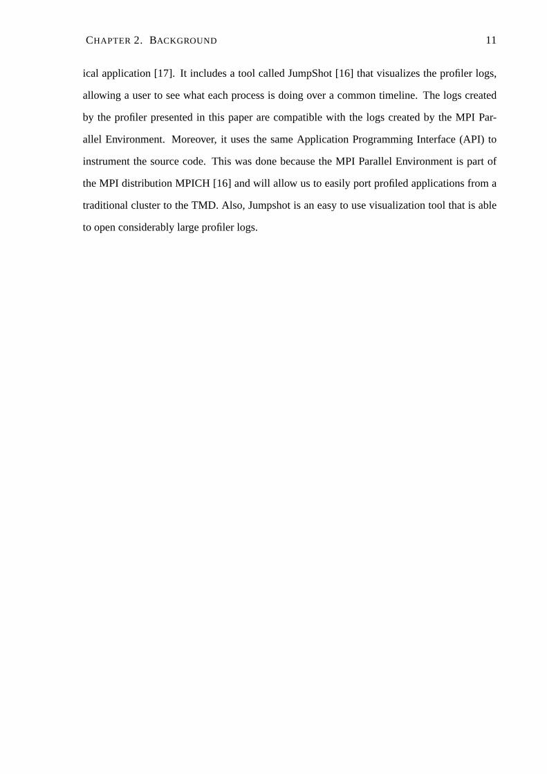
Furthermore, the profiling data does not use any of the communication channels used by the
application, but a special network created exclusively forthe profiler.
Fig. 3.1 shows the high-level profiler architecture betweena User FPGA and a Control
FPGA, and Fig. 3.2 shows the connections between the profilerand the computation nodes.
Each FPGA contains a 64-bit clock cycle counter, shown in Fig. 3.1, synchronized between
all FPGAs. This counter serves as a global timer and is used toobtain the timestamps of
events of interest on the system. The Tracers in Fig. 3.3 are the connection point between
CHAPTER 3. PROFILER 14
the application and the profiler, and each node will have up tothree Tracers, depending on
whether the computation is being profiled or not. This numberof Tracers is needed because
of the parallel nature of hardware where at any given moment anode could be simultaneously
computing, sending and receiving. This may also be true for aPowerPC or Microblaze when
using a TMD-MPE unit.
From Cycle
Counter
PPC
PLB
MPE
Tracer
RX
Tracer
TX
DCR2FSL
Bridge
Tracer
Comp
To Gather
MPE
Tracer
RX
Tracer
TX
Tracer
Comp
To Gather
a)
b)
From Cycle
Counter
From Cycle
Counter
GPIO
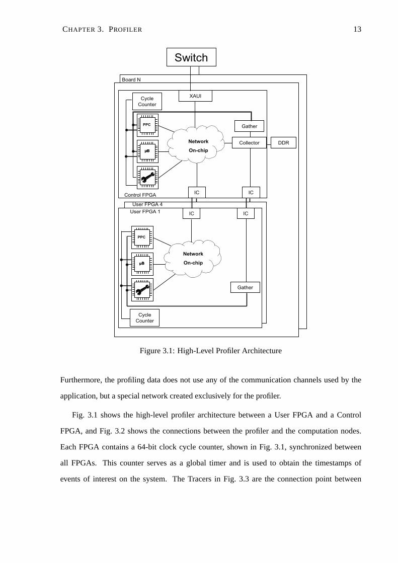
Figure 3.2: a) Processor Profiler Architecture b) Hardware Engine Profiler Architecture
The profiling data of a given instance of a state is kept in the Tracer until that instance
finishes. Only then is the data sent, as one packet through theprofiler network. This is done
to prevent inconsistencies in the profiler data by assuring that either all data referenced to an
instance is saved in memory, or that instance is completely discarded.
The Tracers are non-intrusive with the exception of when they are used on a processor,
since communication from the processor to the tracer is donethrough an FSL and General
Purpose Input/Output (GPIO), delaying the main computation on the processor. However,
when profiling only the computation, the overhead is not significant due to the computation
time itself.
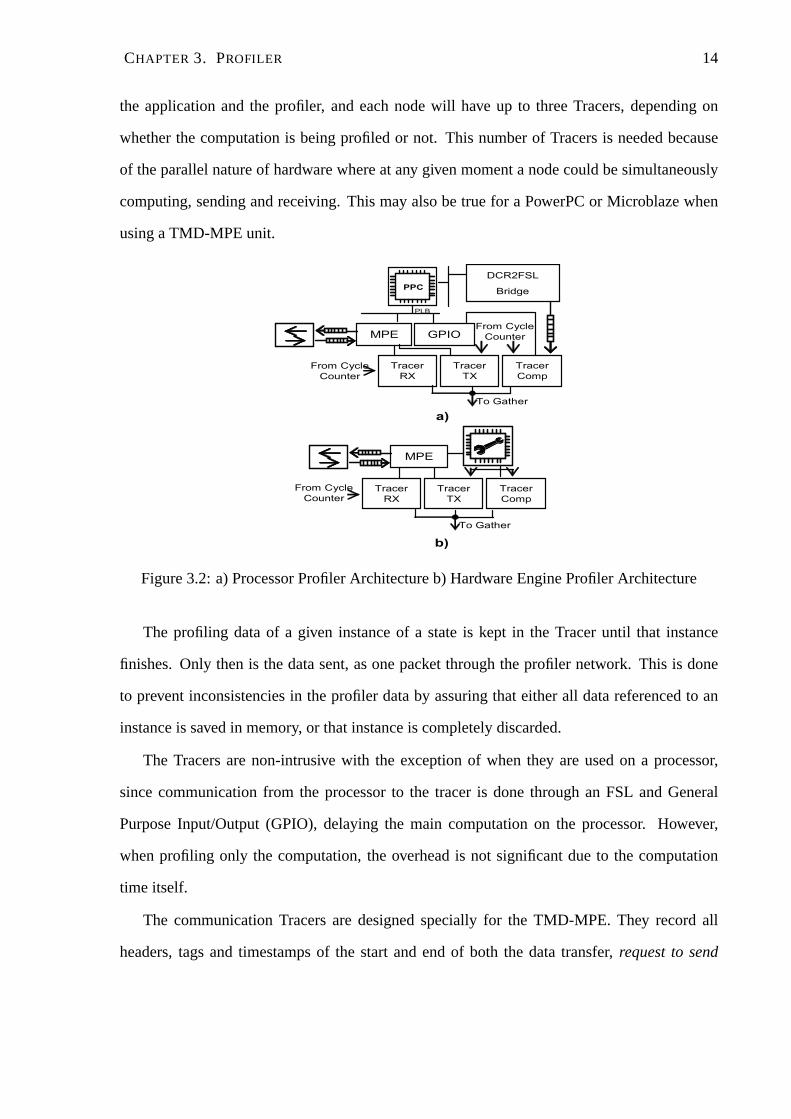
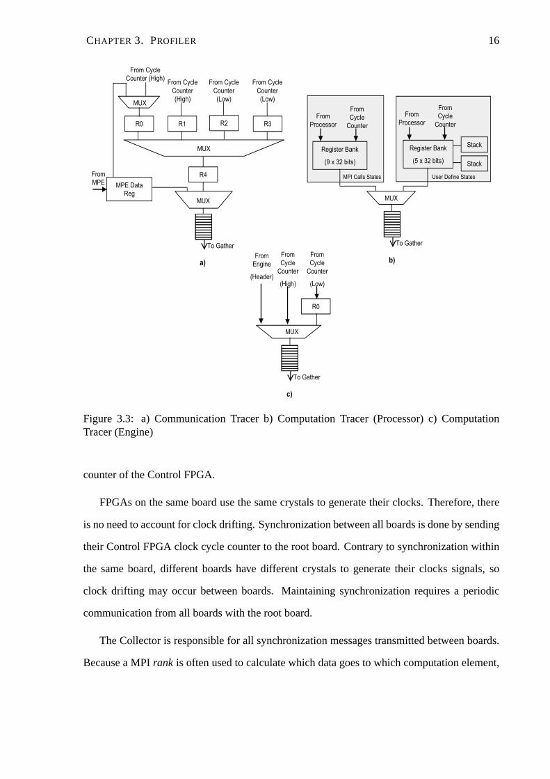
The communication Tracers are designed specially for the TMD-MPE. They record all
headers, tags and timestamps of the start and end of both the data transfer,request to send

CHAPTER 3. PROFILER 15
packets andacknowledgepackets in their registers and FIFO, shown in Fig. 3.3 a). Thecom-
putation Tracers, shown in Fig. 3.3 b), only register the timestamps of the start and end of
user-defined states, except when used in conjunction with a processor (e.g.MicroBlaze, Pow-
erPC) without TMD-MPE, where they will also register all MPI calls. For the latter case, the
computation Tracers have one set of registers for the MPI calls, and one set of registers and two
stacks for the user-defined states. The two sets of registersallow profiling of MPI calls using
user-defined states and the two stacks allow nested user-defined states. Sampling of events of
interest in the hardware engines is done by computation Tracers built specially for each specific
hardware engine. Fig. 3.3 c) shows a generic version of such atracer capable of fulfilling the
profiling needs of most engines.
All Tracers connect to the Gather unit, shown in Fig. 3.1, that will serve as a multiplexor
to send the data to the Control FPGA. On the Control FPGA side, the Collector core, shown
in Fig. 3.1, will receive data from the other FPGAs and from any core being profiled in the
Control FPGA, and will write it to the DDR.
Instrumentation of the hardware is all done at the HDL level.As of now, Tracers and all
cores related with the profiler are manually introduced by the user.
3.2 Clock Counter Synchronization
Synchronization between FPGAs on the same board is done by releasing their reset signals
simultaneously. This can be achieved by having two separatereset signals on the Control
FPGA: one to reset all logic needed to load the User FPGAs, andthe other to reset all cores
connected to the MPI network. The latter is controlled usingGPIO from within the Control
FPGA, and then propagated to the User FPGAs using one of the direct communication lines
existent between them. A latency is associated to the propagation of the reset signal from the
Control FPGA to the User FPGA. This latency is added to the profiling timestamps of the User
FPGAs to assure tight synchronization between their clock cycle counters and the clock cycle
CHAPTER 3. PROFILER 16
R0 R1 R2 R3
R4
MPE Data
Reg
From Cycle
Counter
(High)
From Cycle
Counter (High)From Cycle
Counter
(Low)
From Cycle
Counter
(Low)
MUX
MUX
MUX
To Gather
From
MPE
Register Bank
(9 x 32 bits)
From
Processor
From
Cycle
Counter
MUX
Register Bank
(5 x 32 bits)
Stack
Stack
From
Processor
From
Cycle
Counter
To Gather
MPI Calls States User Define States
a) b)
MUX
To Gather
c)
R0
From
Cycle
Counter
(Low)
From
Engine
(Header)
From
Cycle
Counter
(High)
Figure 3.3: a) Communication Tracer b) Computation Tracer (Processor) c) ComputationTracer (Engine)
counter of the Control FPGA.
FPGAs on the same board use the same crystals to generate their clocks. Therefore, there
is no need to account for clock drifting. Synchronization between all boards is done by sending
their Control FPGA clock cycle counter to the root board. Contrary to synchronization within
the same board, different boards have different crystals togenerate their clocks signals, so
clock drifting may occur between boards. Maintaining synchronization requires a periodic
communication from all boards with the root board.
The Collector is responsible for all synchronization messages transmitted between boards.
Because a MPIrank is often used to calculate which data goes to which computation element,
CHAPTER 3. PROFILER 17
and increasing the total number ofranksmay increase hardware overhead, collectors do not
have a MPIrankassociated to them. However, they still use the MPI infrastructure to send syn-
chronization messages between boards by assuming therank of a nearby computation element
when injecting messages into the network. Similarly, the collectors monitor all messages sent
to thatrankand remove the synchronization ones, identified by a reserved tag. No computation
element is ever aware of this process.
The timestamps are updatedpost-mortem. It’s important to remove any communication
overhead of the synchronization packages, so the time it took to deliver the messages is not
introduced as clock drifting. The first time the synchronization occurs, the root board replies
to all other boards so the round trip time can be calculated. This value is then used for all
subsequent synchronizations. Because the round trip time can increase considerably if the
synchronization message encounters traffic, synchronization messages are sent more often than
needed, and ignored if the calculated drift is too high.
3.3 Software
The profiler library uses the same API as the MPI Parallel Environment of the MPICH distri-
bution. Therefore, an instrumented source code, through embedded calls, can be easily ported
from a traditional cluster to the TMD. However, some of the functions perform a different task
or no task and exist only for portability reasons.MPE Describestate[16] is an example of
such a function. Its task is to allow the user to define a state through two integers, a description
and a color. To support this function it would be necessary for the computation elements to
send these descriptions through the profiler network. This would create unnecessary traffic
from a PowerPC or a Microblaze, and is impossible to support by a hardware engine that runs
no source code. Therefore, all states are described in a configuration file, outside the TMD sys-
tem. The system outputs the profiler logs in text format, which are then concatenated together.
The amalgamated file is then sorted by time (from oldest to recent) and written in the CLOG2
CHAPTER 3. PROFILER 18
format used by the MPI Parallel Environment. The CLOG2 files will then be converted into
SLOG2 (Scalable LOGfile), a format optimized for visualization, and used by Jumpshot4.
User states are created using embedded calls on the application code. States related with
the TMD-MPI are already created within the TMD-MPI library and can be enabled through a
flag at compilation time (only applicable if a soft-processor is not using TMD-MPE).
Chapter 4
Case Studies
In this chapter, the functionality of the profiler is tested using four different case studies. The
first two, Barrier and the heat equation, are simple applications included only to show how the
profiler is able to demonstrate the communication patterns of a given application, running in
software. The third case study, Linpack benchmark, is a demanding application both at the
computation and communication levels used to rank supercomputers on the TOP500 list [18].
It also demonstrates the profiler being used with hardware engines. Finally, the last case study
exposes a bottleneck that would pass unnoticible without a profiling tool.
4.1 Barrier
The barrier is a collective call in which no node will advanceuntil all nodes have reached the
barrier and it is used when the application requires synchronization points. This thesis demon-
strates two versions: a sequential barrier and a binary treebarrier. For the sequential barrier the
root node will wait for all other nodes to report to it and willthen reply to all nodes so they can
advance with the computation. This method scales very poorly as there will be a large amount
of contention while the nodes communicate with the root node. For the binary tree version a
node will report to its parent when its children finish reporting to it, assuring that when the root
node gets a message, all other nodes have reached the barrier. The root node will then signal its
19
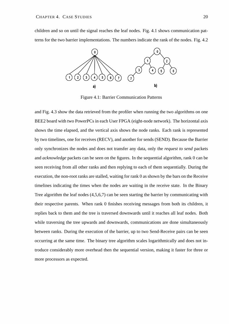
CHAPTER 4. CASE STUDIES 20
children and so on until the signal reaches the leaf nodes. Fig. 4.1 shows communication pat-
terns for the two barrier implementations. The numbers indicate the rank of the nodes. Fig. 4.2
0
1 2
3 4 5 6
7
0
1 2 3 4 5 6 7
a) b)
0
1 2
3 4 5 6
7
0
1 2
3 4 5 6
7
0
1 2 3 4 5 6 7
0
1 2 3 4 5 6 7
a) b)
Figure 4.1: Barrier Communication Patterns
and Fig. 4.3 show the data retrieved from the profiler when running the two algorithms on one
BEE2 board with two PowerPCs in each User FPGA (eight-node network). The horizontal axis
shows the time elapsed, and the vertical axis shows the node ranks. Each rank is represented
by two timelines, one for receives (RECV), and another for sends (SEND). Because the Barrier
only synchronizes the nodes and does not transfer any data, only the request to sendpackets
andacknowledgepackets can be seen on the figures. In the sequential algorithm, rank 0 can be
seen receiving from all other ranks and then replying to eachof them sequentially. During the
execution, the non-root ranks are stalled, waiting for rank0 as shown by the bars on the Receive
timelines indicating the times when the nodes are waiting inthe receive state. In the Binary
Tree algorithm the leaf nodes (4,5,6,7) can be seen startingthe barrier by communicating with
their respective parents. When rank 0 finishes receiving messages from both its children, it
replies back to them and the tree is traversed downwards until it reaches all leaf nodes. Both
while traversing the tree upwards and downwards, communications are done simultaneously
between ranks. During the execution of the barrier, up to twoSend-Receive pairs can be seen
occurring at the same time. The binary tree algorithm scaleslogarithmically and does not in-
troduce considerably more overhead then the sequential version, making it faster for three or
more processors as expected.

CHAPTER 4. CASE STUDIES 21
Figure 4.2: Barrier implemented sequentially
Figure 4.3: Barrier implemented as a binary tree
CHAPTER 4. CASE STUDIES 22
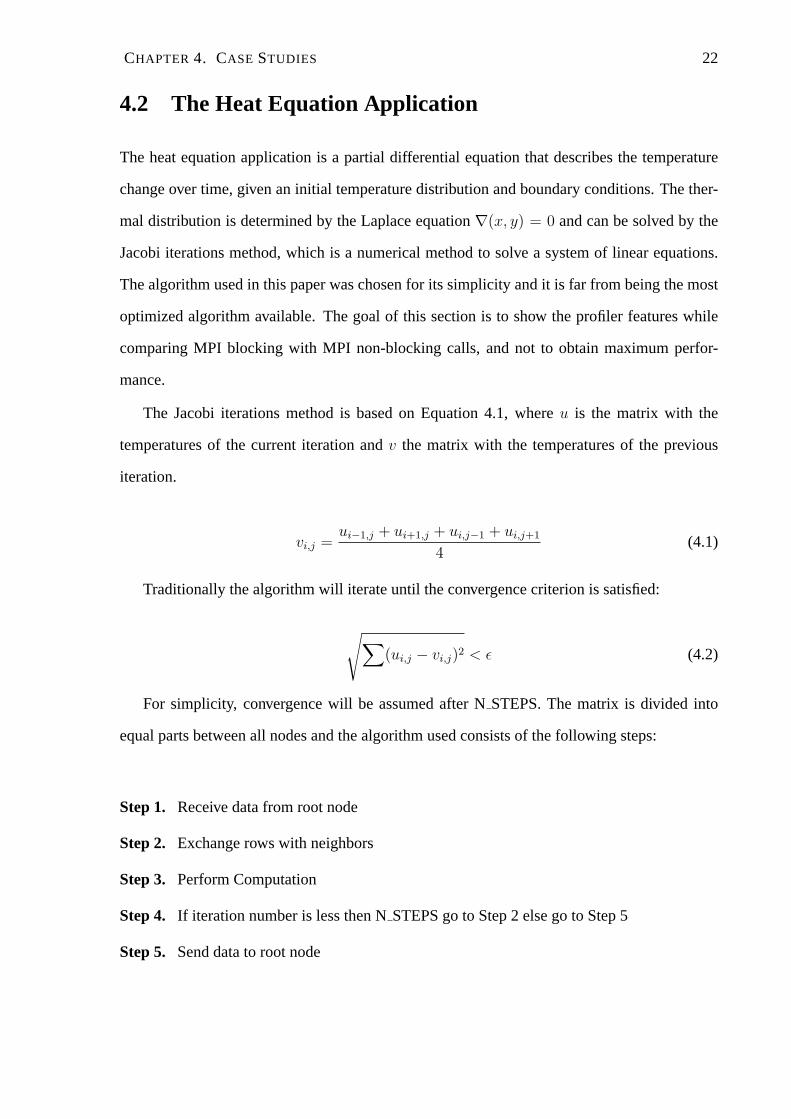
4.2 The Heat Equation Application
The heat equation application is a partial differential equation that describes the temperature
change over time, given an initial temperature distribution and boundary conditions. The ther-
mal distribution is determined by the Laplace equation∇(x, y) = 0 and can be solved by the
Jacobi iterations method, which is a numerical method to solve a system of linear equations.
The algorithm used in this paper was chosen for its simplicity and it is far from being the most
optimized algorithm available. The goal of this section is to show the profiler features while
comparing MPI blocking with MPI non-blocking calls, and notto obtain maximum perfor-
mance.
The Jacobi iterations method is based on Equation 4.1, whereu is the matrix with the
temperatures of the current iteration andv the matrix with the temperatures of the previous
iteration.
vi,j =ui−1,j + ui+1,j + ui,j−1 + ui,j+1
4(4.1)
Traditionally the algorithm will iterate until the convergence criterion is satisfied:
√
∑
(ui,j − vi,j)2 < ǫ (4.2)
For simplicity, convergence will be assumed after NSTEPS. The matrix is divided into
equal parts between all nodes and the algorithm used consists of the following steps:
Step 1. Receive data from root node
Step 2. Exchange rows with neighbors
Step 3. Perform Computation
Step 4. If iteration number is less then NSTEPS go to Step 2 else go to Step 5
Step 5. Send data to root node

CHAPTER 4. CASE STUDIES 23
Fig. 4.4 shows the data decomposition of the global matrix, and which rows are exchanged
between neighbors. Only the first and last row of each of the smallest matrix depends on data
from the neighbors matrices. Other algorithms exist that take into account extra levels of rows
to calculate the new temperatures, but only a first order algorithm was implemented in this
work.
Exchange
Rows
Rank 0
Rank 1
Rank N
Figure 4.4: Data decomposition and point-to-point communication in Jacobi algorithm
MPI supports both blocking and non-blocking calls. Non-blocking calls can be extremely
useful when there is computation that carries no data dependence with the data to be trans-
ferred. If the system architecture allows, the computationcan then be done simultaneously
with the data transfer. However, depending on the implementation, non-blocking calls can
bring extra overhead and care is needed to decide when it is advantageous to use them over the
blocking calls. Parallel systems like the TMD can take full advantage of such calls. Each node
can have a TMD-MPE core that will be in charge of the communications, freeing the CE to
perform whatever computation there may be.
We implemented two different versions for the calculation of the heat equation that differ
only on the type of communication used in Step 2. When using blocking calls, the nodes will
CHAPTER 4. CASE STUDIES 24
stall computation while rows are exchanged between neighbours, regardless of having indepen-
dent rows that can be calculated while waiting for the row exchange. The non-blocking calls
on the other hand, will allow computation of all independentrows on each node after initiating
the row transfers, improving the computation to communication ratio. Both versions of the
application were run with a matrix of 32 by 512, with NSTEPS = 64, on one BEE2 board with
two PowerPCs in each User FPGA. The profiler log for the versionusing the blocking calls can
be seen in Fig. 4.5, and using the non-blocking calls in Fig. 4.6. The hardware configuration
is the same as the previous case study. However, for this example we also instrumented the
source code to visualize the processor computations. Therefore, each rank is now represented
by three timelines, receives (RECV), computation (COMP) and sends (SEND). The profiler
log visualization of the blocking version shows a clear break of computation while the rows
are exchanged between processors. Although the program is being run in parallel across mul-
tiple nodes, each node is running sequentially, such that receives, sends and computation never
overlap. The non-blocking version, on the other hand, takesfull advantage of the communi-
cation infrastructure, and while the TMD-MPE performs the communications, the PowerPC
is computing all independent data. This can be seen on the profiler log visualization of the
non blocking version, where the majority of the ranks are receiving, sending and computing
simultaneously.

CHAPTER 4. CASE STUDIES 25
Figure 4.5: Using blocking calls
Figure 4.6: Using non-blocking calls

CHAPTER 4. CASE STUDIES 26
4.3 The LINPACK Benchmark
The LINPACK benchmark [19] consists of subroutines used to analyze and solve systems
of linear equations. Such systems are solved through matrices calculated by using matrix
decomposition.
LINPACK was originally written in FORTRAN and used to solve systems of linear equa-
tion of size 100 by 100. In 1979, the LINPACK User’s Guide [20] included the performance
data gathered from the most widely used computers of the time. Since then, LINPACK as
been evolving to adapt to the ever changing reality of computer performance. The default
matrix size was increased to 1000 by 1000, reflecting the increase of computer performance.
Also, with the increase of processor frequencies without a comparable increase of memory
frequencies, memories became more and more a bottleneck. Hierarchical memory structures,
where closer memories to the processor are faster, were design to shorten this gap. However,
the closer the memory is to the processor, the smaller it is. If data cannot be found in the
highest hierarchical level memory (cache miss), the application can suffer penalties on the or-
der of hundreds or thousands of cycles. To prevent this, memory management policies can
take advantage of the concept of locality of reference, where, if a given location in memory
is being referenced, then chances are that memory locationsaround it my also be referenced
(Spatial Locality), or, that memory space may be referencedagain in the near future (Tempo-
ral Locality). LINPACK, initially implemented using LEVEL 1BLAS [21] subroutines that
do all calculations as vector-vector, was subsequently implemented using LEVEL 2 BLAS and
LEVEL 3 BLAS subroutines that do vector-matrix and matrix-matrix calculations respectively.
This allows maximization of data reuse by fetching blocks ofdata containing those matrices.
Ax = b (4.3)
Equation 4.3 describes the linear system to be solved. The first step is to perform anLU
decomposition with partial pivoting of matrixA obtaining:
CHAPTER 4. CASE STUDIES 27
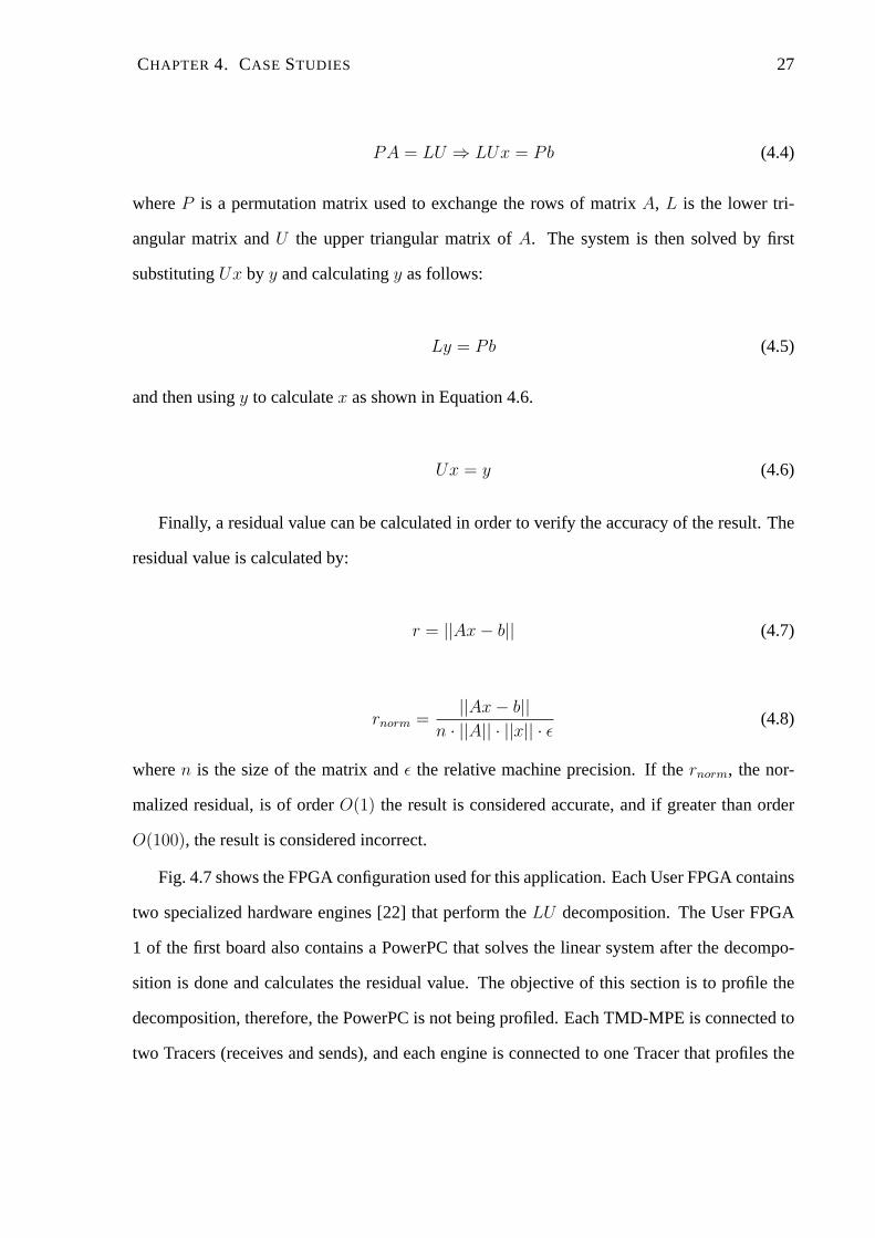
PA = LU ⇒ LUx = Pb (4.4)
whereP is a permutation matrix used to exchange the rows of matrixA, L is the lower tri-
angular matrix andU the upper triangular matrix ofA. The system is then solved by first
substitutingUx by y and calculatingy as follows:
Ly = Pb (4.5)
and then usingy to calculatex as shown in Equation 4.6.
Ux = y (4.6)
Finally, a residual value can be calculated in order to verify the accuracy of the result. The
residual value is calculated by:
r = ||Ax − b|| (4.7)
rnorm =||Ax − b||
n · ||A|| · ||x|| · ǫ(4.8)
wheren is the size of the matrix andǫ the relative machine precision. If thernorm, the nor-
malized residual, is of orderO(1) the result is considered accurate, and if greater than order
O(100), the result is considered incorrect.
Fig. 4.7 shows the FPGA configuration used for this application. Each User FPGA contains
two specialized hardware engines [22] that perform theLU decomposition. The User FPGA
1 of the first board also contains a PowerPC that solves the linear system after the decompo-
sition is done and calculates the residual value. The objective of this section is to profile the
decomposition, therefore, the PowerPC is not being profiled. Each TMD-MPE is connected to
two Tracers (receives and sends), and each engine is connected to one Tracer that profiles the
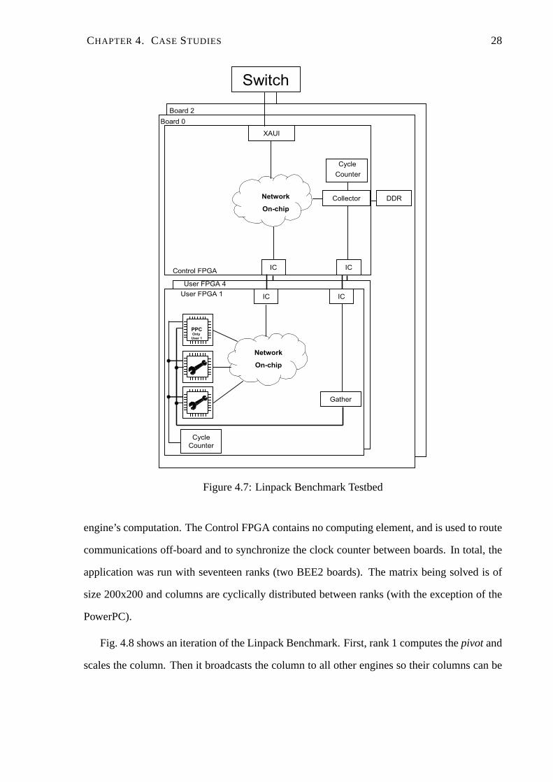
CHAPTER 4. CASE STUDIES 28
XAUI
Collector
IC IC
PPC Only
User 1
Gather
ICIC
DDR
Control FPGA
User FPGA 1
User FPGA 4
Board 2
Switch
Cycle
Counter
Cycle
Counter
Network
On-chip
Network
On-chip
Board 0
Figure 4.7: Linpack Benchmark Testbed
engine’s computation. The Control FPGA contains no computing element, and is used to route
communications off-board and to synchronize the clock counter between boards. In total, the
application was run with seventeen ranks (two BEE2 boards). The matrix being solved is of
size 200x200 and columns are cyclically distributed between ranks (with the exception of the
PowerPC).
Fig. 4.8 shows an iteration of the Linpack Benchmark. First, rank 1 computes thepivotand
scales the column. Then it broadcasts the column to all otherengines so their columns can be
CHAPTER 4. CASE STUDIES 29
Table 4.1: State’s DurationRANK MPI Recv MPI Send ComputationEngines 67% 6.5% 23.6%
updated. Looking at Fig. 4.8, rank 1 spends most of the time sending to other ranks, meaning
that the Broadcast is taking longer then the computation itself. Because of that, all ranks
besides the last four idle considerably waiting for rank 1 tofinish its computation. A larger
matrix would reduce this problem by increasing the computation state. However, because the
application has to be prepared for all sizes of matrices, a solution for this delay would be
to implement the Broadcast in a similar fashion as the Barrier in Section 4.1. This would
reduce the Broadcast length and consequently the iteration length by more then half. Another
noticeable delay can be seen between the starting point of the computation of rank 8 and rank
9, which is double the delay between rank 7 and rank 8. This delay can be attributed to the
off-chip communications through the XAUI interface. Rank 9 is the first rank on the second
BEE2 board.
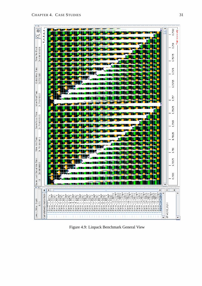
Fig. 4.9 shows a general view (32 iterations) of the Linpack Benchmark. The cyclic distri-
bution of columns between ranks can be seen by the constant exchange of which rank is doing
the Broadcast. Table 4.1 shows the average percentage of timeeach state is active.

CHAPTER 4. CASE STUDIES 30
Figure 4.8: Linpack Benchmark Iteration
CHAPTER 4. CASE STUDIES 31
Figure 4.9: Linpack Benchmark General View
CHAPTER 4. CASE STUDIES 32
4.4 TMD-MPE - Unexpected Messages Queue
When a computing element uses the TMD-MPE, almost all communication overhead of send-
ing/receiving messages is transfered to the TMD-MPE. Independent of using blocking or non-
blocking calls, a message is only sent by a rank after it receives the acknowledge of the other
rank. If a request is made while the receiving rank is occupied with a transaction, this request
needs to be recorded so it can then be replied to when its turn comes. These requests are saved
in a queue called theUnexpected Messages Queue. When a computing element issues a re-
ceive, the TMD-MPE will first check itsUnexpected Messages Queuefor matches. If a match
is found, that entry is taken out of the queue, the queue is reorganized and the TMD-MPE will
process the receive.
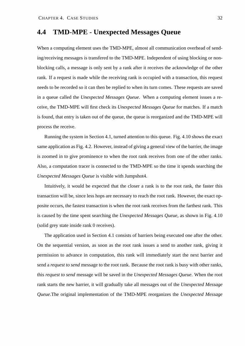
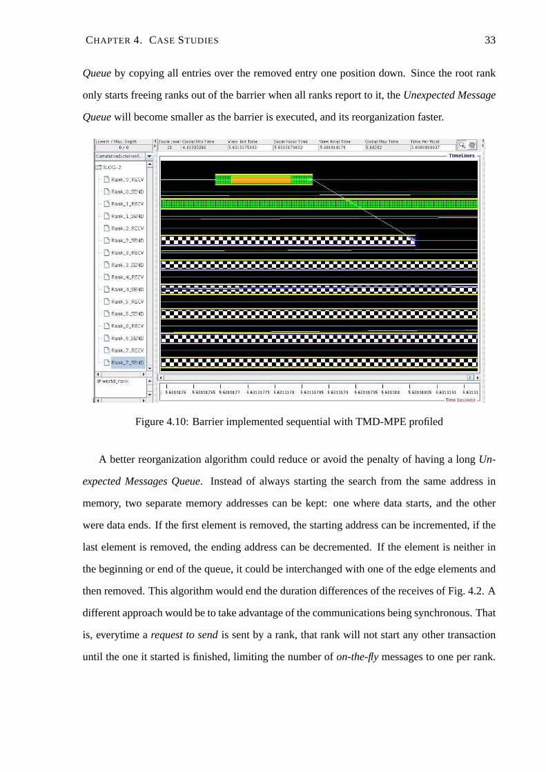
Running the system in Section 4.1, turned attention to this queue. Fig. 4.10 shows the exact
same application as Fig. 4.2. However, instead of giving a general view of the barrier, the image
is zoomed in to give prominence to when the root rank receivesfrom one of the other ranks.
Also, a computation tracer is connected to the TMD-MPE so thetime it spends searching the
Unexpected Messages Queueis visible with Jumpshot4.
Intuitively, it would be expected that the closer a rank is tothe root rank, the faster this
transaction will be, since less hops are necessary to reach the root rank. However, the exact op-
posite occurs, the fastest transaction is when the root rankreceives from the farthest rank. This
is caused by the time spent searching theUnexpected Messages Queue, as shown in Fig. 4.10
(solid grey state inside rank 0 receives).
The application used in Section 4.1 consists of barriers being executed one after the other.
On the sequential version, as soon as the root rank issues a send to another rank, giving it
permission to advance in computation, this rank will immediately start the next barrier and
send arequest to sendmessage to the root rank. Because the root rank is busy with other ranks,
this request to sendmessage will be saved in theUnexpected Messages Queue. When the root
rank starts the new barrier, it will gradually take all messages out of theUnexpected Message
Queue.The original implementation of the TMD-MPE reorganizes the Unexpected Message
CHAPTER 4. CASE STUDIES 33
Queueby copying all entries over the removed entry one position down. Since the root rank
only starts freeing ranks out of the barrier when all ranks report to it, theUnexpected Message
Queuewill become smaller as the barrier is executed, and its reorganization faster.
Figure 4.10: Barrier implemented sequential with TMD-MPE profiled
A better reorganization algorithm could reduce or avoid thepenalty of having a longUn-
expected Messages Queue. Instead of always starting the search from the same addressin
memory, two separate memory addresses can be kept: one wheredata starts, and the other
were data ends. If the first element is removed, the starting address can be incremented, if the
last element is removed, the ending address can be decremented. If the element is neither in
the beginning or end of the queue, it could be interchanged with one of the edge elements and
then removed. This algorithm would end the duration differences of the receives of Fig. 4.2. A
different approach would be to take advantage of the communications being synchronous. That
is, everytime arequest to sendis sent by a rank, that rank will not start any other transaction
until the one it started is finished, limiting the number ofon-the-flymessages to one per rank.

CHAPTER 4. CASE STUDIES 34
If only one request package exists, then all of them can be kept inside theUnexpected Mes-
sages Queueindexed by the rank number and associated to a flag that would validate or not the
content of that index. Searching and removing the element would take one cycle, decreasing
considerably the time each one of those receives take.
Chapter 5
Profiler Overhead
All applications, with the exception of the Linpack benchmark, were executed with the same
hardware configuration. While the hardware overhead introduced by the profiler for the Control
FPGA is constant throughout this work, on the User FPGAs the difference arises from the
Tracers used to profile the PowerPCs, and the Tracers used to profile the hardware engines.
Table 5.1 shows the resource overhead of using the profiler for all configurations where the
percentages in brackets are fractions of a Virtex II Pro 70 FPGA. Part of this overhead is due
to the Tracer’s buffers on the User FPGA and the collector’s buffer on the Control FPGA. The
size of these buffers can be reduced to save resources, however, profiling events may be lost,
compromising part of the profiling data. Another option would be to use BRAMs for buffering,
reducing the size of the cores. Unfortunately, BRAMs can be a scarce resource depending on
the design, so we chose not to use them on the profiler. More specifically, each communication
Tracer occupies 526 LUTs and 1000 flip flops. A Tracer for a processor will occupy 1196
LUTs and 1521 flip flops when profiling both communications andcomputation (no TMD-
MPE), and 855 LUTs and 1200 flip flops when profiling just computation. The overhead of a
computation Tracer for a hardware engine will depend on the hardware engine itself because
each event being captured may require some custom logic to make the event available to the
Tracers. However, the one used for this work is capable of fulfilling the profiling needs of most
35

CHAPTER 5. PROFILER OVERHEAD 36
Table 5.1: Tracers OverheadFPGA LUTS Flip Flops BRAMsControl 3856 (5%) 1279 (1%) 0 (0%)
User 4079 (6.1%) 6630 (10%) 0 (0%)User Linpack 3285 (4.9%) 5366 (8.1%) 0 (0%)
engines. This particular computation Tracer will occupy 396 LUTs and 701 flip flops.
The overhead introduced by the software libraries to profilethe source code of the Microb-
laze or the PowerPC consists of communications with an FSL and GPIO, which on average
will take one hundred and fifty cycles per event. As long as theprogrammer takes some care
on choosing the length of the user states, this will not affect performance considerably. If the
communications are being profiled through software, meaning the processors do not have the
aid of a TMD-MPE unit, the system will suffer a performance decline, making the data re-
trieved from the profiler less helpful to improve performance. However, the data can still be
used to study the application’s communication patterns, and when running a system to obtain
maximum performance, all processors will have the aid of a TMD-MPE unit. Profiling the
TMD-MPE or any hardware engine will not affect system performance as long as the system
frequency is maintained. This may not be possible when the FPGAs are close to full utilization
when it becomes more difficult to meet timing during the placement and routing phase of the
FPGA tools.
Chapter 6
Profiler Implementation on Other
Platforms
6.1 Backplane
The Backplane consists of five Amirix AP1100 PCI development boards. Each board has a
Xilinx 2VP100 FPGA with 128 MB of DDR RAM, 4 MB of SRAM, support for high-speed
serial communication channels, two RS232 serial ports, and an Ethernet connector. Each
FPGA board is connected to a 16-slot PCI backplane, which provides power to the FPGA
boards. In addition to the FPGA boards, there is a Pentium 4 card plugged into the backplane
used only for the FPGA configuration and to provide access to I/O peripherals, such as key-
board, mouse, monitor, and a hard disk drive. The operating system running on the Pentium 4
card is Linux. The boards are interconnected by a fully-connected topology of Multi-Gigabit
Transceiver links (MGTs), which are high-speed serial links. Each MGT channel is configured
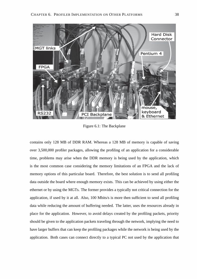
to achieve a full-duplex bandwidth up to 2.5 Gbps. Fig. 6.1 shows an image of the Backplane.
Unlike the BEE2 board, each board on the Backplane only contains one FPGA. Therefore,
each FPGA is responsible for either saving or sending all profiling data generated within it.
While the BEE2 board contains 20 GB of DDR RAM, 4 GB per each FPGA, the Amirix board
37
CHAPTER 6. PROFILER IMPLEMENTATION ON OTHER PLATFORMS 38
FPGA
MGT links
mouse, keyboard& Ethernet
Pentium 4
RS232
Hard DiskConnector
PCI Backplane
Figure 6.1: The Backplane
contains only 128 MB of DDR RAM. Whereas a 128 MB of memory is capable of saving
over 3,500,000 profiler packages, allowing the profiling of an application for a considerable
time, problems may arise when the DDR memory is being used by the application, which
is the most common case considering the memory limitations of an FPGA and the lack of
memory options of this particular board. Therefore, the best solution is to send all profiling
data outside the board where enough memory exists. This can be achieved by using either the
ethernet or by using the MGTs. The former provides a typically not critical connection for the
application, if used by it at all. Also, 100 Mbits/s is more then sufficient to send all profiling
data while reducing the amount of buffering needed. The latter, uses the resources already in
place for the application. However, to avoid delays createdby the profiling packets, priority
should be given to the application packets traveling through the network, implying the need to
have larger buffers that can keep the profiling packages while the network is being used by the
application. Both cases can connect directly to a typical PC not used by the application that

CHAPTER 6. PROFILER IMPLEMENTATION ON OTHER PLATFORMS 39
caries has memory to hold all profiling data of all FPGAs. Fig.6.2 shows the diagram for both
implementations.
Network
On-chip
Pro�ler
Logic
MGT Ethernet
x86 x86
Figure 6.2: Possible Implementation of the Profiler on the Backplane
6.2 HPRC Implementation Platform
This system consists of an Intel 4-Processor Server System S7000FC4UR. One of the sockets
has a Xilinx Accelerated Computing Platform (ACP) consistingof a stack of PCB modules.
The first layer contains the bridge FPGA (XC5VLX110) and is physically placed in one of the
X86 sockets on the motherboard. It provides a connection point to Intel’s Front Side Bus (FSB)
and provides communications for the upper-level layers. The second layer contains two FPGAs
(XC5VLX330) used for computation in the same PCB. All FPGAs are directly connected by
LVDS lines in the same layer and between layers. Another socket has an Intel Quadcore Xeon
processor. The Xilinx ACP platform and the X86s share 8 GB of RAMthrough the FSB, and
the machine is running a standard SMP Linux distribution. Implementing the profiler in this
platform is in part similar to Section 6.1. In both cases, theprofiling packages need to be sent
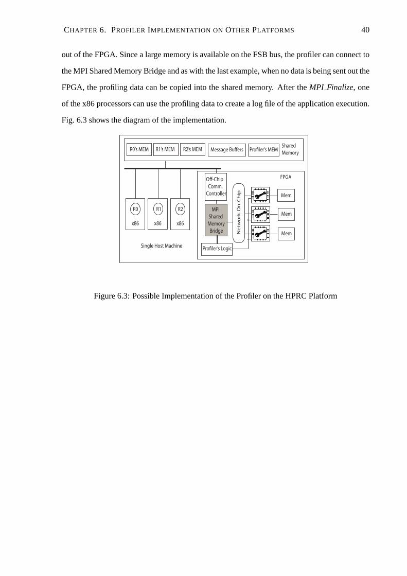
CHAPTER 6. PROFILER IMPLEMENTATION ON OTHER PLATFORMS 40
out of the FPGA. Since a large memory is available on the FSB bus, the profiler can connect to
the MPI Shared Memory Bridge and as with the last example, whenno data is being sent out the
FPGA, the profiling data can be copied into the shared memory.After theMPI Finalize, one
of the x86 processors can use the profiling data to create a logfile of the application execution.
Fig. 6.3 shows the diagram of the implementation.
R0
x86
R1
x86
R2
x86
R1’s MEM R2’s MEMR0’s MEM Message Bu!ers Pro"ler’s MEMShared
Memory
O!-Chip
Comm.
Controller
MPI
Shared
Memory
Bridge
Mem
Mem
MemNe
two
rk-O
n-C
hip
Pro"ler’s Logic
FPGA
Single Host Machine
Figure 6.3: Possible Implementation of the Profiler on the HPRC Platform
Chapter 7
Conclusions
To obtain full performance on FPGA systems, it is necessary to have a complete understanding
of the application to avoid unexpected behavior that may undermine performance. A tool that
allows the user to visualize what each core is executing at a given moment can bring the insight
needed to avoid possible bottlenecks. In this work, we present a profiler that not only allows
that knowledge to be retrieved from the system, but does so without affecting the performance
of the system significantly. All major features of the profiling software environment provided
by MPICH were implemented on a FPGA system.
First, the profiler is used in two simple case studies: a barrier and a heat equation application
using the Jacobi iterations method. In both of them we are able to demonstrate the communi-
cation patterns and can use that knowledge to improve the application either by changing the
algorithm to a more scalable one or by using more suitable communications calls so all levels
of parallelism provided by the hardware can be used. Also, a bottleneck was found and cor-
rected on the TMD-MPE that, without the profiler, would most likely pass unnoticed. Finally,
the profiler is used to study the behavior of the Linpack benchmark, and is able to point to
bottlenecks that reduce performance considerably.
The reconfigurability of FPGAs allows us to instantiate onlythe necessary hardware for
performance analysis, minimizing the hardware overhead. Moreover, that hardware runs par-
41

CHAPTER 7. CONCLUSIONS 42
allel with the main application, and becomes intrusive onlywhen communication resources
are shared, or when the system frequency is not mantained. Performance analysis on reconfig-
urable hardware also increases the number of events available to the user, since unlike software
profiling, we’re not limited to events related with a processor. Our scope is now the full hard-
ware system and we can accurately profile network componentsin addition to CEs. Compat-
ibility with an existing profiling software environment reduces the learning curve of this tool
and allows comparisons between traditional clusters and reconfigurable systems-on-chip.
This type of performance analysis (post-mortem) works well for applications with constant
behavior throughout their execution. The profiler is able toaid the designer achieve a better net-
work topology, better algorithms and even improve some hardware engines. For an application
which behavior varies, the profiler can aid with building a system based on initial conditions.
Overall, it provides a good starting point for performance analysis on the TMD system.
Chapter 8
Future Work
With this working profiler the next step will be to focus on other computing demanding ap-
plications besides the Linpack benchmark that contain morecomplex communication patterns
(e.g. molecular dynamics). With the increase in complexityof the applications, a tool that can
perform a pre-analysis of the data and identify possible bottleneck areas can become extremely
useful.
Improvements on the hardware blocks to reduce their footprint and increase functionality,
such as track critical messages, are also scheduled.
Microblaze and PowerPC computation is being profiled intrusively through an FSL and
GPIO connection. To avoid this penalty, the Tracer can profiler computation by accessing
the program counter of each of the processors using a similarmethod as SnoopP or Xilinx
Microblaze Trace Core (XMTC) [13].
Porting the profiler into the HPRC implementation presented in Chapter 6 will also be done
in the near future.
At the moment, all analysis is being donepost-mortem. Another option would be to im-
plement a profiler that would be more restricted in the amountand type of data that it could
retrieve, allowing real-time analysis for systems with dynamic behavior. Such profiler could
work in conjunction with the one presented in this paper, where one would be used to optimize
43

CHAPTER 8. FUTURE WORK 44
the initial configuration of the system, and the other to adapt the system to dynamic behavior.

Chapter 9
Appendixes
9.1 Appendix A
In this appendix, an example system is provided and the interface of each hardware block is
explained.
9.1.1 Example System
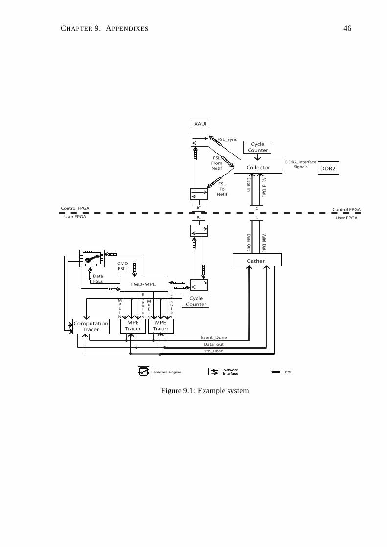
Fig. 9.1 shows the connections between different blocks of the profiler. This example consid-
ers only one engine being profiled in the User FPGA. Both communication and computation
are being profiled. Fig. 9.1 can be use as reference for Section. 9.1.2, Section. 9.1.3 and Sec-
tion. 9.1.4
45
CHAPTER 9. APPENDIXES 46
TMD-MPE
MPE
Tracer
Gather
Collector
Valid_D
ata
Data_In
Valid_D
ata
Data_O
ut
IC
IC
DDR2
DDR2_Interface
Signals
MPE
TracerComputation
Tracer
Cycle
Counter
IC
IC
XAUI
Cycle
Counter
Event_Done
Data_out
FSL
From
NetIf
FSL
To
NetIf
FSL_Sync
Control FPGA
User FPGA
Control FPGA
User FPGA
Network
Interface
Network
InterfaceHardware Engine FSL
CMD
FSLs
Data
FSLs
MPEIN
Enables
Enables
Fifo_Read
MPEIN
Figure 9.1: Example system
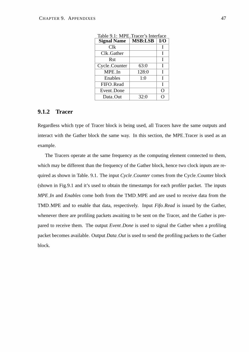
CHAPTER 9. APPENDIXES 47
Table 9.1: MPETracer’s InterfaceSignal Name MSB:LSB I/O
Clk IClk Gather I
Rst ICycle Counter 63:0 I
MPE In 128:0 IEnables 1:0 I
FIFO Read IEventDone ODataOut 32:0 O
9.1.2 Tracer
Regardless which type of Tracer block is being used, all Tracers have the same outputs and
interact with the Gather block the same way. In this section,the MPETracer is used as an
example.
The Tracers operate at the same frequency as the computing element connected to them,
which may be different than the frequency of the Gather block, hence two clock inputs are re-
quired as shown in Table. 9.1. The inputCycleCountercomes from the CycleCounter block
(shown in Fig.9.1 and it’s used to obtain the timestamps for each profiler packet. The inputs
MPE In andEnablescome both from the TMDMPE and are used to receive data from the
TMD MPE and to enable that data, respectively. InputFifo Read is issued by the Gather,
whenever there are profiling packets awaiting to be sent on the Tracer, and the Gather is pre-
pared to receive them. The outputEventDone is used to signal the Gather when a profiling
packet becomes available. OutputData Out is used to send the profiling packets to the Gather
block.

CHAPTER 9. APPENDIXES 48
Table 9.2: Gather InterfaceSignal Name MSB:LSB I/O
Clk IRst I
Data In (33*N PROFILERS-1:0 IEventDone N PROFILERS-1:0 I
FIFO ReadTracers N PROFILERS-1:0 OSendingData O
DataOut 32:0 O
9.1.3 Gather
Table 9.2 shows all Gather block ports. The Gather block retrieves all profiling data from the
Tracers and sends it to the Control FPGA. InputsData In andEventDoneare the concatenated
data of all TracersData Out andEventDoneoutputs, respectively. OutputFifo ReadTracers
is the concatenated read signals for each Tracer FIFO. Output Data Out connects to the In-
terchip andValid Data is enabled when that data is valid. Table 9.2 shows all Gatherblock
ports.
CHAPTER 9. APPENDIXES 49
Table 9.3: Collector InterfaceSignal Name MSB:LSB I/O
Clk IInterchipClk I
Rst ICycle Counter 63:0 I
Data in N FPGAS*33-1:0 IValid Data I
Numberof Boards 2:0 IMyrank 7:0 I
Mem Cmd Address 31:0 OMem Cmd RNW OMem Cmd Valid OMem Cmd Tag 31:0 OMem Cmd Ack IMem Wr Din 143:0 OMem Wr BE 17:0 O
FSL S DATA (FROM NETIF) 31:0 IFSL S CTRL (FROM NETIF) I
FSL S EXISTS (FROMNETIF) IFSL S READ (FROM NETIF) OFSL M DATA 0 (FSL SYNC) 31:0 OFSL M CTRL 0 (FSL SYNC) O
FSL M WRITE 0 (FSL SYNC) OFSL M FULL 0 (FSL SYNC) IFSL M DATA 1 (TO NETIF) 31:0 IFSL M CTRL 1 (TO NETIF) I
FSL M EXISTS 1 (TO NETIF) IFSL M READ 1 (TO NETIF) O
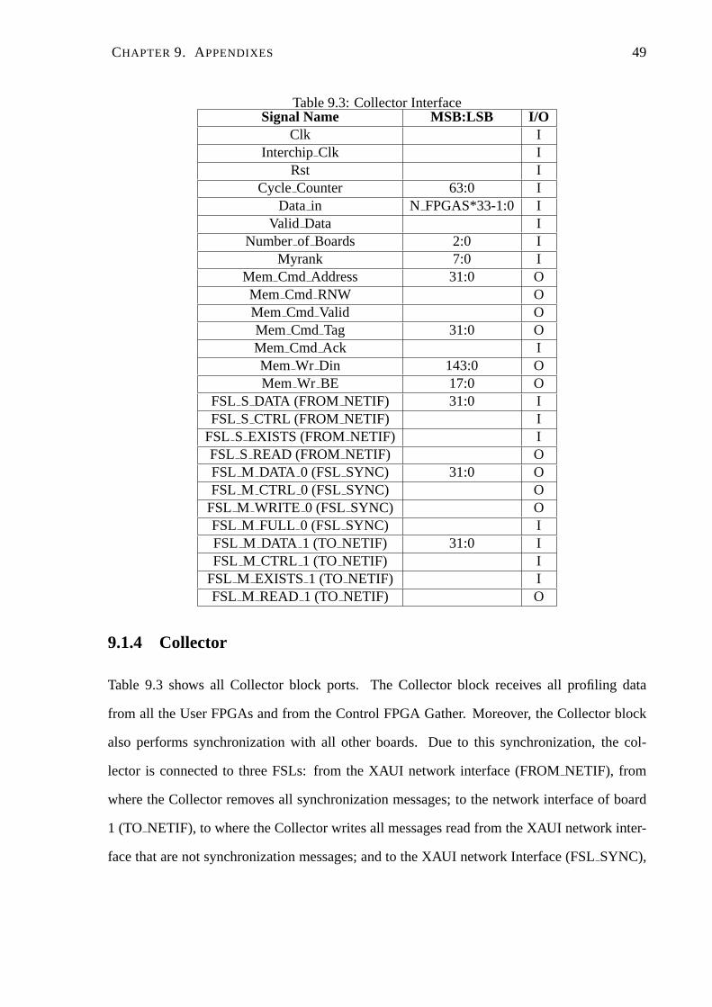
9.1.4 Collector
Table 9.3 shows all Collector block ports. The Collector blockreceives all profiling data
from all the User FPGAs and from the Control FPGA Gather. Moreover, the Collector block
also performs synchronization with all other boards. Due tothis synchronization, the col-
lector is connected to three FSLs: from the XAUI network interface (FROMNETIF), from
where the Collector removes all synchronization messages; to the network interface of board
1 (TO NETIF), to where the Collector writes all messages read from the XAUI network inter-
face that are not synchronization messages; and to the XAUI network Interface (FSLSYNC),
CHAPTER 9. APPENDIXES 50
where the Collector sends all its synchronization messages.Both profiling packets and syn-
chronization packets are saved in the DDR2 memory.
Bibliography
[1] Xtreme Data Inc.http://www.xtremedatainc.com/.
[2] DRC Computer.http://www.drccomputer.com/.
[3] IBM. http://www-01.ibm.com/chips/techlib/techlib.nsf/
products/PowerPC_405_Embedded_Cores.
[4] Arun Patel, Christopher Madill, Manuel Saldana, Christopher, Comis Regis Pomes, and
Paul Chow. A scalable fpga-based multiprocessor. InIn IEEE Symposium on Field-
Programmable Custom Computing Machines (FCCM’06), pages 111–120, April 2006.
[5] Manuel Saldana and Paul Chow. Tmd-mpi: An MPI implementation for multipleproces-
sors across multiple fpgas. InIn IEEE International Conference on Field-Programmable
Logic and Applications (FPL 2006), pages 329–334, August 2006.
[6] Manuel Saldana, Daniel Nunes, Emanuel Ramalho, and Paul Chow. Configurationand
programming of heterogeneous multiprocessors on a multi-fpga system. InIn 3rd Inter-
national Conference on ReConFigurable Computing and FPGAs 2006 (ReConFig’06),
September 2006.
[7] The MPI Forum. MPI: a message passing interface. InSupercomputing ’93: Proceedings
of the 1993 ACM/IEEE conference on Supercomputing, pages 878–883, New York, NY,
USA, 1993. ACM Press.
51
BIBLIOGRAPHY 52
[8] Richard L. Graham and Timothy S.Woodall and Jeffrey M. Squyres. Open mpi: A flex-
ible high performance mpi. InIn Proceedings, 6th Annual International Conference on
Parallel Processing and Applied Mathematics, Poznan, Poland, 2005.
[9] Chen Chang, John Wawrzynek, and Robert W. Brodersen. BEE2: A High-End Reconfig-
urable Computing System.IEEE Des. Test ’05, 22(2):114–125, 2005.
[10] Seth Koehler, John Curreri, and Alan D. George. Performance analysis challenges and
framework for high-performance reconfigurable computing.Parallel Computing, 34(4-
5):217–230, 2008.
[11] Susan L., Graham Peter, B. Kessler, and Marshall McKusick. Gprof: A call graph exe-
cution profiler. InProceeding of Department of the ACM SIGPLAN 1982 Symposium on
Compiler Construction, Boston, MA, June 1982.
[12] Browne S., Deane C., Ho G., and Mucci P. Papi: A portable interface to hardware per-
formance counters. InProceedings of Department of Defense HPCMP Users Group
Conference, June 1999.
[13] Xilinx. http://www.xilinx.com/.
[14] Altera. http://www.altera.com/.
[15] Lesley Shannon and Paul Chow. Maximizing system performance using reconfigura-
bility to monitor system communications. InIn International Conference on Field-
Programmable technology (FPT), pages 231–238, Brisbane, Australia, December 2004.
[16] W. Gropp and E. Lusk and N. Doss and A. Skjellum. A High-Performance, Portable
Implementation of the MPI Message Passing Interface Standard. Parallel Computing,
22(6):789–828, 1996.
[17] Adam Leko and Hans Sherburne. MPE/jumpshot evaluation.
BIBLIOGRAPHY 53
[18] Hans Meuer, Erich Strohmaier, Jack Dongarra, and HorstSimon. ”Top500 Supercom-
puter Sites”.http://www.top500.org/.
[19] J. Dongarra, P. Luszczek, and A. Petitet. ”The LINPACK Benchmark: Past, Present and
Future”. http://www.netlib.org/utk/people/JackDongarra/PAPERS/
hpl.pdf.
[20] J. J. Dongarra, C. B. Moler, J. R. Bunch, and G.W. Stewart.”LINPACK Users’ Guide”.
SIAM, 1979.
[21] C. L. Lawson and R. J. Hanson and D. R. Kincaid and F. T. Krogh.Basic Linear Algebra
Subprograms for Fortran Usage.ACM Transactions on Mathematical Software (TOMS),
5(3):308–323, 1979.
[22] Emanuel Ramalho.The LINPACK Benchmark on a Multi-Core Multi-FPGA System,
Department of Electrical & Computer Engineering, University of Toronto, Master Thesis,
2008.