Archvied in

http://dspace.nitrkl.ac.in/dspace

http://dx.doi.org/10.1002/ceat.200700065

Published in

Chemical Engineering & Technology, 2007, Volume 30, Issue 12 , Pages 1659 - 1665

A Process Integration based Approach for the Analysis of Evaporator System

S. Khanam1*, B. Mohanty2

1Lecturer, Department of Chemical Engineering, National Institute of Technology Rourkela

Rourkela – 769 008, Orissa, (India)

2Professor, Department of Chemical Engineering, Indian Institute of Technology Roorkee

Roorkee – 247 667, Uttaranchal, (India)

email: S. Khanam (shabinahai@gmail.com, skhanam@nitrkl.ac.in)

*Correspondence to S. Khanam, 1Department of Chemical Engineering, National Institute of

Technology Rourkela, Rourkela – 769 008, Orissa, (India)

Abstract

A scalable new mathematical model based on the principles of Process Integration has been developed

for the analysis of multiple effect evaporator (MEE) systems. It uses the concepts of stream analysis,

temperature path and internal heat exchange for the formulation of model equations. In addition to

above the model also takes into account variable physico-thermal properties of steam/vapor,

condensate and liquor while simulating the MEE system.

The present model consists of a set of linear equations and does not pose any stability or oscillation

problems during solution as is generally seen in the case of models which are based on sets of non-

linear equations. The model equations are automatically generated through the computer program. To

prove the utility of the present model it was run for three different liquor and flow sequences. The

results thus obtained are compared with published models.

Keywords: Mathematical modeling. Stream analysis. Temperature path. Internal heat exchange

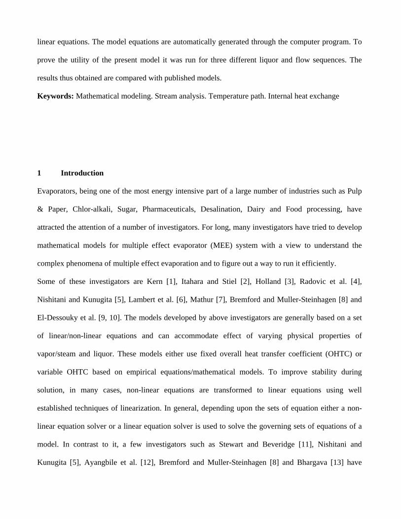
1 Introduction

Evaporators, being one of the most energy intensive part of a large number of industries such as Pulp

& Paper, Chlor-alkali, Sugar, Pharmaceuticals, Desalination, Dairy and Food processing, have

attracted the attention of a number of investigators. For long, many investigators have tried to develop

mathematical models for multiple effect evaporator (MEE) system with a view to understand the

complex phenomena of multiple effect evaporation and to figure out a way to run it efficiently.

Some of these investigators are Kern [1], Itahara and Stiel [2], Holland [3], Radovic et al. [4],

Nishitani and Kunugita [5], Lambert et al. [6], Mathur [7], Bremford and Muller-Steinhagen [8] and

El-Dessouky et al. [9, 10]. The models developed by above investigators are generally based on a set

of linear/non-linear equations and can accommodate effect of varying physical properties of

vapor/steam and liquor. These models either use fixed overall heat transfer coefficient (OHTC) or

variable OHTC based on empirical equations/mathematical models. To improve stability during

solution, in many cases, non-linear equations are transformed to linear equations using well

established techniques of linearization. In general, depending upon the sets of equation either a non-

linear equation solver or a linear equation solver is used to solve the governing sets of equations of a

model. In contrast to it, a few investigators such as Stewart and Beveridge [11], Nishitani and

Kunugita [5], Ayangbile et al. [12], Bremford and Muller-Steinhagen [8] and Bhargava [13] have

preferred to use iterative techniques for the solution of their models. In most of the cases, these

solution techniques exhibit convergence and instability problems [13].

With the development of Process Integration (PI) principles investigators also tried to analyze the

complex MEE system with the help of these. Since 1986, a considerable amount of work has been

carried out on the integration of MEE system with back ground process by Kemp [14], MacDonald

[15], Smith and Linnhoff [16] and Westphalen and Wolf Maciel [17], etc. Westerberg and Hillenbrand

[18] used the concepts of PI in MEE system to optimize operating temperature of evaporator and to

select optimal feed flow sequence. However, they did not demonstrate it through examples of complex

MEE system generally encountered in industries. On the other hand, though the PI based methods

provide useful insights to the problem and suggest remedial measures to improve it have not been

developed to full extent so that these could be used to tackle all complexities of the MEE process.

Thus, under the above backdrop it appears that there is a scope for development of a simple PI based

model which can be used for the analysis of a MEE system. The present paper uses three primary

concepts of Westerberg and Hillenbrand [18], which are multiple hypothetical streams in a feed,

temperature path and internal heat exchange. These basic principles are developed to an extent where

by these can be used to formulate a simple mathematical model, to be used as an analysis tool for

MEE systems. The model is scaleable and can accommodate the practical complexities of the

industrial MEE systems. This model is composed of linear algebraic equations and can be solved by

any linear equation solver. It also does not offer any instability and convergence problem. However,

in this paper the most simplified model is presented to establish the basic concepts.

2 Problem Statement

As the present work establishes a new concept it was thought logical to demonstrate it with the help of

a simple triple effect evaporator (TEE) system with forward feed flow sequence rather than taking up a

full blown MEE system generally used in industries. The schematic diagram of the TEE system is

shown in Fig. 1. Live steam of amount, Ws, enters into the steam chest of the first effect at

temperature, T0, and exits it as a condensate stream CS (where, Ws = CS) after supplying latent heat

for vaporization to the first effect. The vapor generated in the first effect is moved to the vapor chest of

the second effect and causes evaporation in this effect. This sequence is repeated up to third effect.

Feed first enters into effect no. 1 and then follows the forward sequence.

In the present model it is assumed that the feed stream is composed of a number of individual streams

such as condensate streams which subsequently come out from different effects (except first as it

utilizes live steam) and a product stream. The feed stream, in virtual sense, is composed of four

streams namely: one product stream, P, and three condensate streams designated as, C1, C2 and C3.

Initially, the four streams, P, C1, C2 and C3, enter to the first effect at feed temperature, TF. The water

content of the liquor is evaporated and vapor stream “V1” is created which is fed to effect No. 2 where

it gives heat and converts in to a condensate stream “C1” and exits the effect. The remaining streams

are now P, C2 and C3. These streams exit the first effect at a temperature T1 and enter effect No. 2,

which is then gets evaporated in this effect and vapor stream “V2” is generated. It is sent to the vapor

chest of effect No.3 for heating and it finally comes out in the form of a condensate stream “C2” from

3rd effect. Finally, the remaining streams, P and C3, move to effect no. 3 from where the condensate

stream “C3” gets separated. Finally, the product stream “P” comes out from effect No.3.

To trace the levels of temperature a particular stream acquires while it exchanges sensible heat and

traverses from entry effect to exit effect (sequence of entry and exit depends on flow sequence) the

concept of “temperature path” is used. It is defined as a “Path followed by the temperatures of a

stream when it passes through an effect or a network of it”. In the present case, it plays a vital role in

the development of model equations. The temperature paths of all four constituent streams of feed are

shown in Fig. 2 in which T1, T2 and T3 are vapor body temperatures of 1st, 2nd and 3rd effects,

respectively. The temperature paths are plotted to demonstrate another important concept called

“internal heat exchange”. This concept works on one of the basic principles of PI, called “maximum

energy recovery”. It allows different streams or their part to exchange heat with each other in order to

facilitate maximum amount of heat to be exchanged through internal exchange and thus provides a

mean to compute the minimum possible amount of live steam required by the system.

To demonstrate the concept of “internal heat exchange” let us consider the temperature path of P,

shown in Fig. 2, which first moves upward in temperature from point “a” to “c” through point “b” and

hence behaves as a cold stream. However, the same stream from point “d” to “f” through “e” and “g”

works as a hot stream as its temperature decreases in this temperature path.

When two streams exchange heat it needs a driving force in terms of temperature difference. As per

the concepts of PI let us assume that it needs a minimum temperature difference, ΔTmin, to effect the

transfer. As the product stream “P” behaves as a hot stream in some part of the temperature path and

as a cold stream in remaining path its hot stream part can exchange heat with its cold stream part

subjected to the ΔTmin constraint. For example, the cold stream part of “P”, denoted by “a” to “c”

through “b”, can be heated up from point “a” to “b” by taking heat from hot stream part (“d” to “e”) of

it. This is a feasible heat transfer as the temperature difference between points “d” and “b” and that

between points “e” and “a” is ΔTmin. As a consequence of the heat transfer the temperature of the hot

stream part of “P” drops from “d” to “e”. However, the above referred hot stream can not transfer

further heat to cold stream as it will violate the ΔTmin criterion. Similarly, the temperature of the cold

stream part of “P” can not rise above point “b” which is equal to T1-ΔTmin, while exchanging heat with

the corresponding hot stream as it will violate ΔTmin criterion. Thus, it can be concluded that the

criteria of ΔTmin offers some constraint towards the transfer of heat and all the heat available with hot

stream can’t be transferred to cold stream even if it is in a position to take it (if violation of ΔTmin

constraint is accepted) .

In this case, the stream “P” enters into the first effect at point “b” where it is heated up and reaches up

to the point “c” before gets evaporated. Therefore, in this case, for stream, P, maximum possible

internal heat exchange is equal to [P*CPP*(TF-T1+ΔTmin)] kW where CPP is the specific heat capacity

of product. In other words, this is equal to the amount of heat needed for heating “P” from point “a” to

“b”. The remaining part i.e. “b” to “c” will require heating by hot utility and similarly the part “e” to

“g” will require cold utility for cooling. This is also possible that the required heating from “b” to “c”

will be provided inside the evaporator through steam/vapor. The requirement of cold utility can be

eliminated in this case if the stream enters the effect at the state of “e” and then flashes inside to reach

to a temperature corresponding to “g”. Similarly, the amount of feasible internal heat exchange for

other streams namely C1, C2 and C3 can be computed from temperature path diagram, Fig. 2. For the

development of model the temperature of feed is taken as T2.

3 Model Development

It is a well known fact the mathematical model use thermo-physical properties to describe the identity

of a process. In this case, as an example, the water has been selected as the evaporating fluid. The

thermo-physical properties of the feed also considered based on the case study selected for

comparison.

3.1 Development of Correlations for Physical Properties of Steam and Condensates

For development of correlations for heat of vaporization and enthalpy of condensate (water in present

case), data are taken from standard text of Smith et al. [19] and two different forth order polynomial in

temperature are fitted. Further, correlation obtained for enthalpy of condensate is differentiated with

respect to temperature to get the correlation of specific heat capacity of condensate. Correlations thus

developed are tabulated in Tab. 1.

3.2 Development of a Simplified Mathematical Model for the TEE System

A model is developed for a TEE system shown in Fig. 1 with forward flow sequence which is then

modified and extended to accommodate other flow sequence depending upon the Case Study selected

for comparison. Following assumptions are made to cut down the complexity of the model: (1)

Constant driving force exists in all effects. (2) Vapor leaving an effect is at equilibrium with liquor and

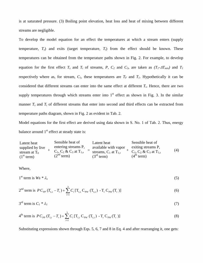
is at saturated pressure. (3) Boiling point elevation, heat loss and heat of mixing between different

streams are negligible.

To develop the model equation for an effect the temperatures at which a stream enters (supply

temperature, Ts) and exits (target temperature, Tt) from the effect should be known. These

temperatures can be obtained from the temperature paths shown in Fig. 2. For example, to develop

equation for the first effect Ts and Tt of streams, P, C2 and C3, are taken as (T1-ΔTmin) and T1

respectively where as, for stream, C1, these temperatures are TF and T1. Hypothetically it can be

considered that different streams can enter into the same effect at different Ts. Hence, there are two

supply temperatures through which streams enter into 1st effect as shown in Fig. 3. In the similar

manner Ts and Tt of different streams that enter into second and third effects can be extracted from

temperature paths diagram, shown in Fig. 2 as evident in Tab. 2.

Model equations for the first effect are derived using data shown in S. No. 1 of Tab. 2. Thus, energy

balance around 1st effect at steady state is:

+ = + (4)

Where,

1st term is Ws * λs (5)

2nd term is )] (TCT - )(T CT[)( rPWrs1,PWs1,

3

1,1 ∑

=

+−i

irsPP CTTCP (6)

3rd term is C1 * λ1 (7)

4th term is )] (TCT - )(T CT[)( rPWrt1,PWt1,

3

1,1 ∑

=

+−i

irtPP CTTCP (8)

Substituting expressions shown through Eqs. 5, 6, 7 and 8 in Eq. 4 and after rearranging it, one gets:

Latent heat supplied by live stream at T0 (1st term)

Sensible heat of entering streams P, C1, C2 & C3 at T1,s (2nd term)

Latent heat available with vapor streams, C1 at T1,t (3rd term)

Sensible heat of exiting streams P, C1, C2 & C3 at T1,t (4th term)

(9)

Where, )] (TCT - )(T C[T t1,PWt1,s1,PWs1,1 =b

Putting the values of T1,s and T1,t from Tab. 2, following equations for first effect is obtained:

(10)

Where, )] (TCT - )(T C[T 1PW1FPWF1 =b and )] (TCT - )T-(T C)T-[(T 1PW1min1PWmin12 ΔΔ=b

Similarly, equation for effect no. 2 and 3 can be developed as shown below:

Second effect:

0)(

12

min

2

33

2

32

2

11 =

Δ+⎥

⎦

⎤⎢⎣

⎡+⎥

⎦

⎤⎢⎣

⎡−+⎥

⎦

⎤⎢⎣

⎡λλλλ

λ TCPbC

bCC PP (11)

Where, )] (TCT - )(T C)[(T 2PW2min2PWmin23 TTb Δ+Δ+=

Third effect:

0)(

13

32

3

43

3

22 =

−+⎥

⎦

⎤⎢⎣

⎡−+⎥

⎦

⎤⎢⎣

⎡λλλ

λ TTCPbCC PP (12)

Where, )] (TCT - )(T C[T 3PW32PW24 =b

Overall mass balance around the TEE system provides:

PFCi

i −=∑=

3

1 (13)

Thus, simplified model for TEE system consists of four linear equations, Eqs. 10 to 13. The above

model can also be written as a scalable model in terms of “n”- number of effects [20].

4 Solution of the Model

The present model consists of a set of four linear algebraic equations, Eqs. 10 to 13. It is not out of

place to mention that similar non PI based models contain 9 number of equations for the above system.

0)(

11

,1,1

1

13

11

=−

+⎥⎦

⎤⎢⎣

⎡−+⎥

⎦

⎤⎢⎣

⎡∑= λλλ

λ tsPP

ii

s TTCPbCWs

0)(111

min

1

23

21

11

1

=Δ−

+⎥⎦

⎤⎢⎣

⎡−+⎥

⎦

⎤⎢⎣

⎡−+⎥

⎦

⎤⎢⎣

⎡∑= λλλλ

λ TCPbCbCWs PP

ii

s

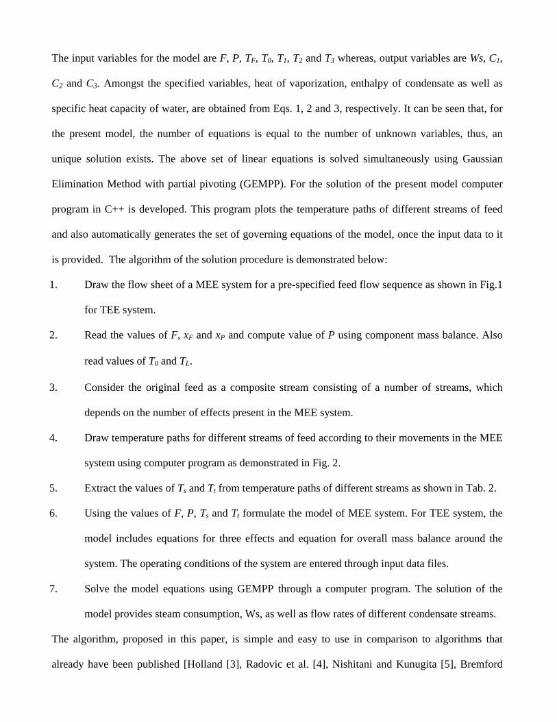
The input variables for the model are F, P, TF, T0, T1, T2 and T3 whereas, output variables are Ws, C1,

C2 and C3. Amongst the specified variables, heat of vaporization, enthalpy of condensate as well as

specific heat capacity of water, are obtained from Eqs. 1, 2 and 3, respectively. It can be seen that, for

the present model, the number of equations is equal to the number of unknown variables, thus, an

unique solution exists. The above set of linear equations is solved simultaneously using Gaussian

Elimination Method with partial pivoting (GEMPP). For the solution of the present model computer

program in C++ is developed. This program plots the temperature paths of different streams of feed

and also automatically generates the set of governing equations of the model, once the input data to it

is provided. The algorithm of the solution procedure is demonstrated below:

1. Draw the flow sheet of a MEE system for a pre-specified feed flow sequence as shown in Fig.1

for TEE system.

2. Read the values of F, xF and xP and compute value of P using component mass balance. Also

read values of T0 and TL.

3. Consider the original feed as a composite stream consisting of a number of streams, which

depends on the number of effects present in the MEE system.

4. Draw temperature paths for different streams of feed according to their movements in the MEE

system using computer program as demonstrated in Fig. 2.

5. Extract the values of Ts and Tt from temperature paths of different streams as shown in Tab. 2.

6. Using the values of F, P, Ts and Tt formulate the model of MEE system. For TEE system, the

model includes equations for three effects and equation for overall mass balance around the

system. The operating conditions of the system are entered through input data files.

7. Solve the model equations using GEMPP through a computer program. The solution of the

model provides steam consumption, Ws, as well as flow rates of different condensate streams.

The algorithm, proposed in this paper, is simple and easy to use in comparison to algorithms that

already have been published [Holland [3], Radovic et al. [4], Nishitani and Kunugita [5], Bremford

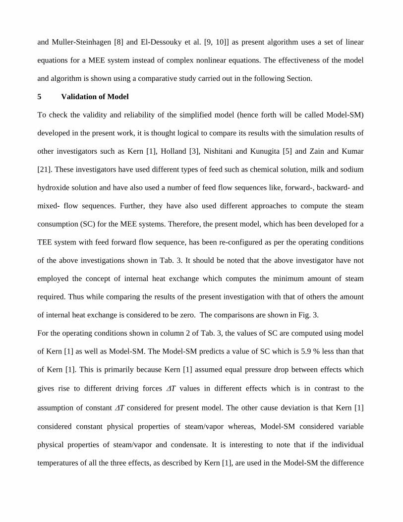
and Muller-Steinhagen [8] and El-Dessouky et al. [9, 10]] as present algorithm uses a set of linear

equations for a MEE system instead of complex nonlinear equations. The effectiveness of the model

and algorithm is shown using a comparative study carried out in the following Section.

5 Validation of Model

To check the validity and reliability of the simplified model (hence forth will be called Model-SM)

developed in the present work, it is thought logical to compare its results with the simulation results of

other investigators such as Kern [1], Holland [3], Nishitani and Kunugita [5] and Zain and Kumar

[21]. These investigators have used different types of feed such as chemical solution, milk and sodium

hydroxide solution and have also used a number of feed flow sequences like, forward-, backward- and

mixed- flow sequences. Further, they have also used different approaches to compute the steam

consumption (SC) for the MEE systems. Therefore, the present model, which has been developed for a

TEE system with feed forward flow sequence, has been re-configured as per the operating conditions

of the above investigations shown in Tab. 3. It should be noted that the above investigator have not

employed the concept of internal heat exchange which computes the minimum amount of steam

required. Thus while comparing the results of the present investigation with that of others the amount

of internal heat exchange is considered to be zero. The comparisons are shown in Fig. 3.

For the operating conditions shown in column 2 of Tab. 3, the values of SC are computed using model

of Kern [1] as well as Model-SM. The Model-SM predicts a value of SC which is 5.9 % less than that

of Kern [1]. This is primarily because Kern [1] assumed equal pressure drop between effects which

gives rise to different driving forces ΔT values in different effects which is in contrast to the

assumption of constant ΔT considered for present model. The other cause deviation is that Kern [1]

considered constant physical properties of steam/vapor whereas, Model-SM considered variable

physical properties of steam/vapor and condensate. It is interesting to note that if the individual

temperatures of all the three effects, as described by Kern [1], are used in the Model-SM the difference

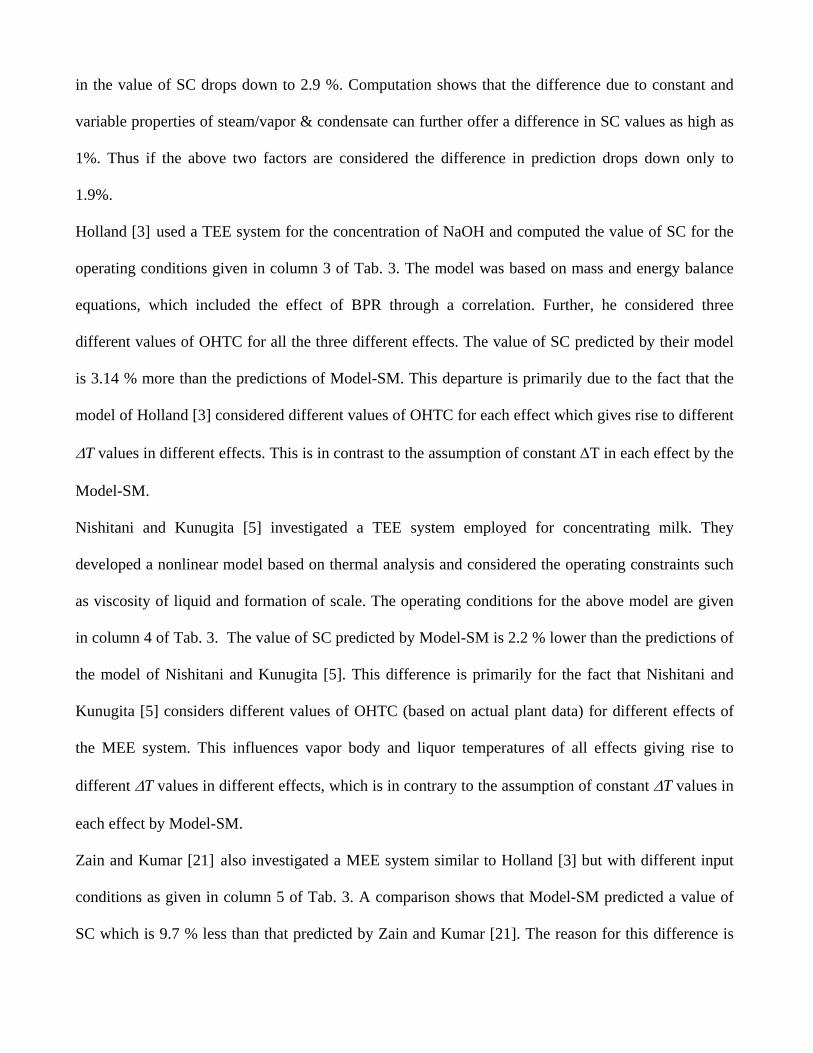
in the value of SC drops down to 2.9 %. Computation shows that the difference due to constant and

variable properties of steam/vapor & condensate can further offer a difference in SC values as high as

1%. Thus if the above two factors are considered the difference in prediction drops down only to

1.9%.

Holland [3] used a TEE system for the concentration of NaOH and computed the value of SC for the

operating conditions given in column 3 of Tab. 3. The model was based on mass and energy balance

equations, which included the effect of BPR through a correlation. Further, he considered three

different values of OHTC for all the three different effects. The value of SC predicted by their model

is 3.14 % more than the predictions of Model-SM. This departure is primarily due to the fact that the

model of Holland [3] considered different values of OHTC for each effect which gives rise to different

ΔT values in different effects. This is in contrast to the assumption of constant ΔT in each effect by the

Model-SM.

Nishitani and Kunugita [5] investigated a TEE system employed for concentrating milk. They

developed a nonlinear model based on thermal analysis and considered the operating constraints such

as viscosity of liquid and formation of scale. The operating conditions for the above model are given

in column 4 of Tab. 3. The value of SC predicted by Model-SM is 2.2 % lower than the predictions of

the model of Nishitani and Kunugita [5]. This difference is primarily for the fact that Nishitani and

Kunugita [5] considers different values of OHTC (based on actual plant data) for different effects of

the MEE system. This influences vapor body and liquor temperatures of all effects giving rise to

different ΔT values in different effects, which is in contrary to the assumption of constant ΔT values in

each effect by Model-SM.

Zain and Kumar [21] also investigated a MEE system similar to Holland [3] but with different input

conditions as given in column 5 of Tab. 3. A comparison shows that Model-SM predicted a value of

SC which is 9.7 % less than that predicted by Zain and Kumar [21]. The reason for this difference is

that Zain and Kumar [21] used empirical correlations for the computation of OHTC as well as BPR of

NaOH for all the three effects. Both the above facts caused the vapor and liquor temperatures of

effects to change considerably. As a result of it values of ΔT are significantly different in all the three

effects which is contrary to the constant ΔT in all effects assumption of the present model, Model-SM.

Further, to substantiate the above explanation for the departure in the values of SC predicted, the

present Model-SM was run by taking the ΔT values computed by Zain and Kumar [21]. As expected

the difference drops down to only 1.7% in this case.

From the above results it can be concluded that the difference in the predictions of values of SC by the

Model-SM and that by others models are within acceptable limits.

5.1 Effect of Internal Heat Exchange

The present model has a provision to include the concept of “internal heat exchange”. Once this

concept is included it predicts the lowest value of SC required conducting the evaporation process.

However, translation of this concept may not be economically viable under the present physical state

of technology. Never-the-less this offers some insight to the efficient use of design and operating

freedoms of a MEE system. With this in mind, Model-SM was run with the provision of “internal heat

exchange” with ΔTmin values equal to 10°C. As per the principles of PI if the value of ΔTmin is

increased it increases the amount of utility required. In other words the value of SC will increase.

Whereas, if ΔTmin is decreased it decreases the value of SC predicted. To show the effect of internal

heat exchange, Tab. 4 is created, which shows the amounts of live steam computed with and without

internal heat exchange for TEE systems considered by Holland [3], Nishitani & Kunugita [5] and Zain

& Kumar [21]. It should be noted that the operating conditions selected by Kern [1] do not offer any

scope for internal heat exchange.

It is clear from Tab. 4 that for the TEE systems taken by Holland [3], Nishitani & Kunugita [5] and

Zain & Kumar [21] the amount of live steam can be reduced by 9.5, 7.4 and 1.1 %, respectively. This

is interesting to note that the extent of reduction in the values of SC is different for different

investigations. This is primarily due to difference in mode of operation of the TEE system, which

offered scope for different amounts of internal heat exchange. The amount of internal heat exchange,

which will take place in a particular mode of operation, is governed by temperature paths of different

streams of feed. To make the above fact clear, for the TEE systems considered by Holland [3],

Nishitani & Kunugita [5] and Zain & Kumar [21] temperature paths are drawn in Figs. A.1, A.2 and

A.3, respectively, which shows that amount of internal heat exchange is maximum for Holland [3] and

minimum for Zain and Kumar [21]. As a result maximum and minimum reductions in SC are observed

for the model of Holland [3] and Zain & Kumar [21], respectively.

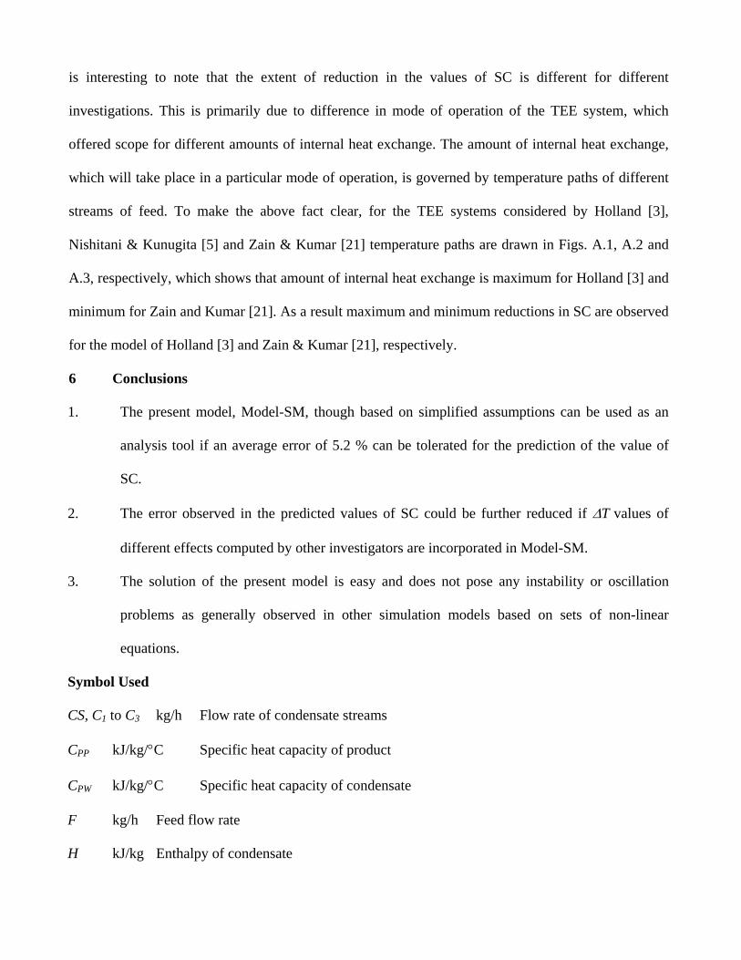
6 Conclusions

1. The present model, Model-SM, though based on simplified assumptions can be used as an

analysis tool if an average error of 5.2 % can be tolerated for the prediction of the value of

SC.

2. The error observed in the predicted values of SC could be further reduced if ΔT values of

different effects computed by other investigators are incorporated in Model-SM.

3. The solution of the present model is easy and does not pose any instability or oscillation

problems as generally observed in other simulation models based on sets of non-linear

equations.

Symbol Used

CS, C1 to C3 kg/h Flow rate of condensate streams

CPP kJ/kg/°C Specific heat capacity of product

CPW kJ/kg/°C Specific heat capacity of condensate

F kg/h Feed flow rate

H kJ/kg Enthalpy of condensate

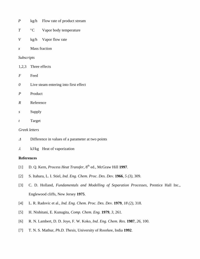
P kg/h Flow rate of product stream

T °C Vapor body temperature

V kg/h Vapor flow rate

x Mass fraction

Subscripts

1,2,3 Three effects

F Feed

0 Live steam entering into first effect

P Product

R Reference

s Supply

t Target

Greek letters

Δ Difference in values of a parameter at two points

λ kJ/kg Heat of vaporization

References

[1] D. Q. Kern, Process Heat Transfer, 8th ed., McGraw Hill 1997.

[2] S. Itahara, L. I. Stiel, Ind. Eng. Chem. Proc. Des. Dev. 1966, 5 (3), 309.

[3] C. D. Holland, Fundamentals and Modelling of Separation Processes, Prentice Hall Inc.,

Englewood cliffs, New Jersey 1975.

[4] L. R. Radovic et al., Ind. Eng. Chem. Proc. Des. Dev. 1979, 18 (2), 318.

[5] H. Nishitani, E. Kunugita, Comp. Chem. Eng. 1979, 3, 261.

[6] R. N. Lambert, D. D. Joye, F. W. Koko, Ind. Eng. Chem. Res. 1987, 26, 100.

[7] T. N. S. Mathur, Ph.D. Thesis, University of Roorkee, India 1992.

[8] D. J. Bremford, H. Muller-Steinhagen, Appita J. 1994, 47 (4), 320.

[9] H. T. El-Dessouky et al., Chem. Eng. Tech. 1998, 21, 15.

[10] H. T. El-Dessouky et al., Trans IChemE. 2000, 78 (Part A), 662.

[11] G. Stewart, G. S. G Beveridge, Comp. Chem. Eng. 1977, 1 (1), 3.

[12] W. O. Ayangbile, E. O. Okeke, G. S. G. Beveridge, Comp. Chem. Eng. 1984, 8 (3/4), 235.

[13] R. Bhargava, Ph.D. Thesis, Indian Institute of Technology Roorkee, India 2004.

[14] I. C. Kemp, J. Sep. Proc. Tech. 1986, 7 (9).

[15] E. MacDonald, Proc. Eng. 1986, 25 (November).

[16] R. Smith, B. Linnhoff, Chem. Eng. Res. Des. 1988, 66, 195.

[17] D. L. Westphalen, M. R. Wolf Maciel, Braz. J. Chem. Eng. 2000, 17 (4-7), 525.

[18] A. W. Westerberg, J. B. Hillenbrand Jr., Comp. Chem. Eng. 1988, 12 (7), 625.

[19] J. M. Smith et al., Introduction to Chemical Engineering Thermodynamics, 4th ed., McGraw

Hill, 2001.

[20] S. Khanam, Ph.D. Thesis, Indian Institute of Technology Roorkee, India 2006.

[21] O. S. Zain, S. Kumar, J. Chem. Eng. Jap. 1996, 29 (5), 889.

Appendix A

Temperature paths of four streams of feed for TEE systems considered by Holland [3], Nishitani &

Kunugita [5] and Zain & Kumar [21] are shown using Figs. A.1, A.2 and A.3, respectively, as given

below:

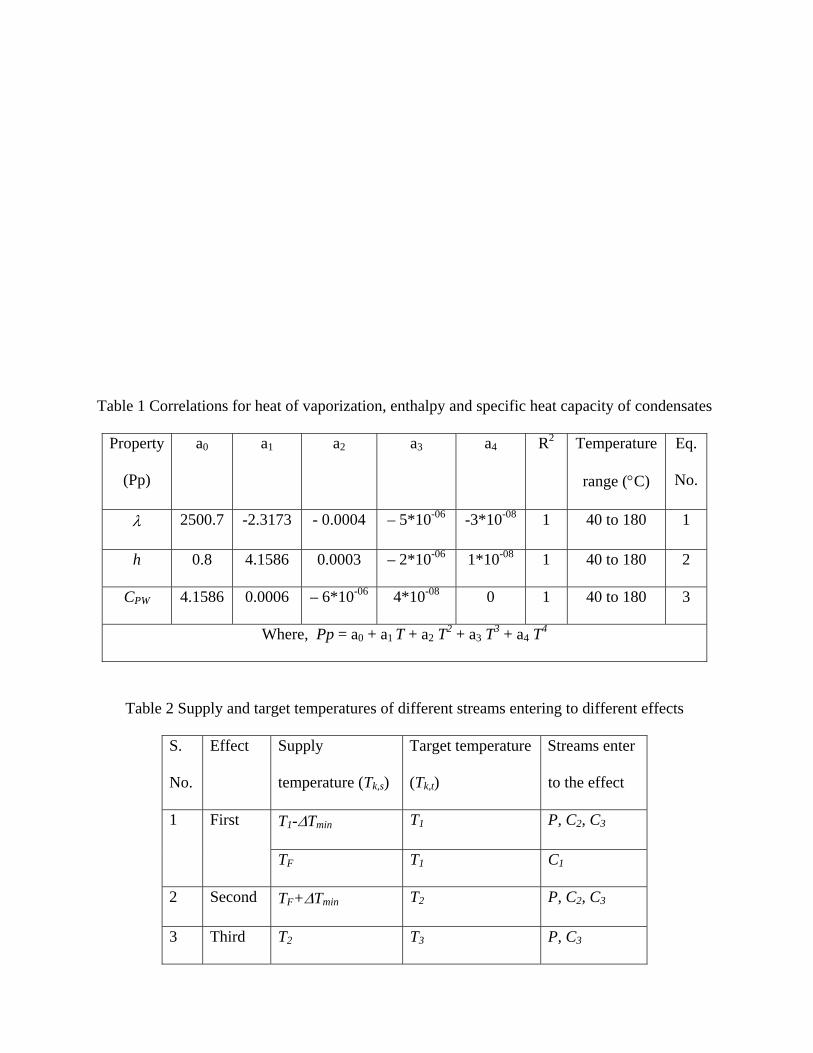
Table 1 Correlations for heat of vaporization, enthalpy and specific heat capacity of condensates

Property

(Pp)

a0 a1 a2 a3 a4 R2 Temperature

range (°C)

Eq.

No.

λ 2500.7 -2.3173 - 0.0004 – 5*10-06 -3*10-08 1 40 to 180 1

h 0.8 4.1586 0.0003 – 2*10-06 1*10-08 1 40 to 180 2

CPW 4.1586 0.0006 – 6*10-06 4*10-08 0 1 40 to 180 3

Where, Pp = a0 + a1 T + a2 T2 + a3 T3 + a4 T4

Table 2 Supply and target temperatures of different streams entering to different effects

S.

No.

Effect Supply

temperature (Tk,s)

Target temperature

(Tk,t)

Streams enter

to the effect

1 First T1-ΔTmin T1 P, C2, C3

TF T1 C1

2 Second TF+ΔTmin T2 P, C2, C3

3 Third T2 T3 P, C3

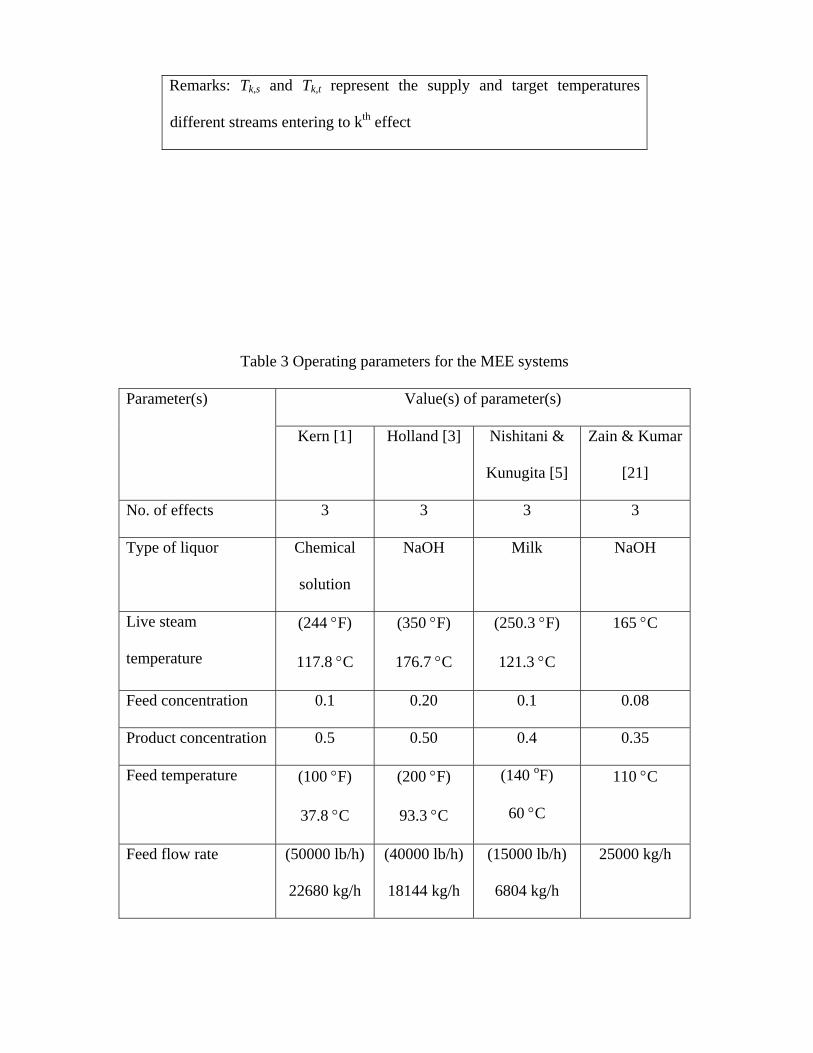
Remarks: Tk,s and Tk,t represent the supply and target temperatures

different streams entering to kth effect

Table 3 Operating parameters for the MEE systems

Parameter(s) Value(s) of parameter(s)

Kern [1] Holland [3] Nishitani &

Kunugita [5]

Zain & Kumar

[21]

No. of effects 3 3 3 3

Type of liquor Chemical

solution

NaOH Milk NaOH

Live steam

temperature

(244 °F)

117.8 °C

(350 °F)

176.7 °C

(250.3 °F)

121.3 °C

165 °C

Feed concentration 0.1 0.20 0.1 0.08

Product concentration 0.5 0.50 0.4 0.35

Feed temperature (100 °F)

37.8 °C

(200 °F)

93.3 °C

(140 oF)

60 °C

110 °C

Feed flow rate (50000 lb/h)

22680 kg/h

(40000 lb/h)

18144 kg/h

(15000 lb/h)

6804 kg/h

25000 kg/h

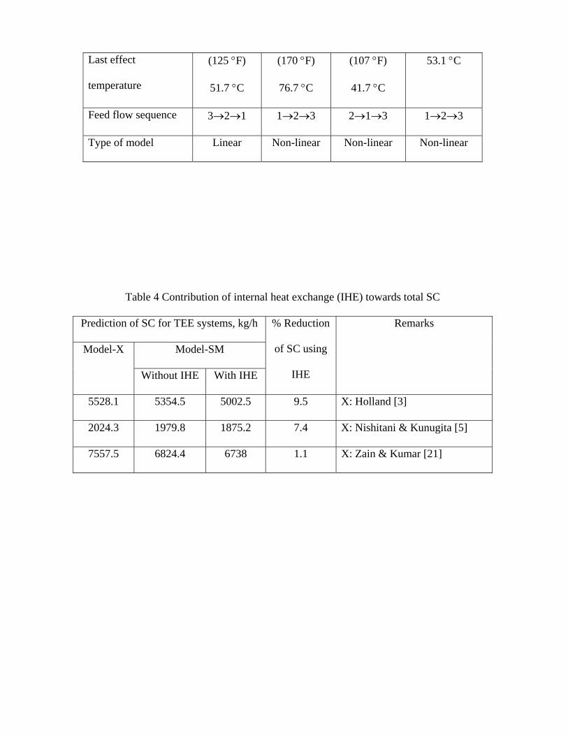
Last effect

temperature

(125 °F)

51.7 °C

(170 °F)

76.7 °C

(107 °F)

41.7 °C

53.1 °C

Feed flow sequence 3→2→1 1→2→3 2→1→3 1→2→3

Type of model Linear Non-linear Non-linear Non-linear

Table 4 Contribution of internal heat exchange (IHE) towards total SC

Prediction of SC for TEE systems, kg/h % Reduction

of SC using

IHE

Remarks

Model-X Model-SM

Without IHE With IHE

5528.1 5354.5 5002.5 9.5 X: Holland [3]

2024.3 1979.8 1875.2 7.4 X: Nishitani & Kunugita [5]

7557.5 6824.4 6738 1.1 X: Zain & Kumar [21]

List of Figures

Figure 1. The schematic diagram of a TEE system

Figure 2. Temperature paths of different streams of feed for a TEE system for forward flow sequence

Figure 3. Comparisons between Model-SM and other models

Figure A.1. Temperature paths of different streams of feed for a TEE system of Holland [3]

Figure A.2. Temperature paths of different streams of feed for a TEE system of Nishitani & Kunugita [5]

Figure A.3. Temperature paths of different streams of feed for a TEE system of Zain & Kumar [21]

List of Tables

Table 1 Correlations for heat of vaporization, enthalpy and specific heat capacity of condensates

Table 2 Supply and target temperatures of different streams entering to different effects

Table 3 Operating parameters for the MEE systems

Table 4 Contribution of internal heat exchange (IHE) towards total SC

Table of contents

1 Introduction

2 Problem Statement

3 Model Development

3.1 Development of Correlations for Physical Properties of Steam and Condensates

3.2 Development of a Simplified Mathematical Model for the TEE System

4 Solution of the Model

5 Validation of Model

5.1 Effect of Internal Heat Exchange

6 Conclusions

Symbol Used

References

Appendix A