A NUMERICAL STUDY OF ENTROPY GENERATION,

HEAT AND MASS TRANSFER IN BOUNDARY LAYER

FLOWS

A THESIS SUBMITTED TO THE UNIVERSITY OF KWAZULU-NATAL

FOR THE DEGREE OF DOCTOR OF PHILOSOPHY

IN THE COLLEGE OF AGRICULTURE, ENGINEERING & SCIENCE

By

Mohammed Hassan Mohammed Almakki

School of Mathematics, Statistics & Computer Science

November 2018

Contents

Abstract iii

Declaration v

Acknowledgments vii

List of Publications ix

1 Introduction 1

1.1 Heat and mass transfer . . . . . . . . . . . . . . . . . . . . . . . . . . . . . . . 3

1.2 Nanofluids . . . . . . . . . . . . . . . . . . . . . . . . . . . . . . . . . . . . . . 5

1.3 Thermal radiation . . . . . . . . . . . . . . . . . . . . . . . . . . . . . . . . . . 7

1.4 Entropy generation . . . . . . . . . . . . . . . . . . . . . . . . . . . . . . . . . . 8

1.5 Unsteady flows . . . . . . . . . . . . . . . . . . . . . . . . . . . . . . . . . . . . 9

1.6 Methods of solution . . . . . . . . . . . . . . . . . . . . . . . . . . . . . . . . . 10

1.6.1 The spectral relaxation method . . . . . . . . . . . . . . . . . . . . . . . 12

1.6.2 The spectral and bivariate quasilinearization methods . . . . . . . . . . 14

i

1.7 Thesis objectives . . . . . . . . . . . . . . . . . . . . . . . . . . . . . . . . . . . 15

1.8 Thesis structure . . . . . . . . . . . . . . . . . . . . . . . . . . . . . . . . . . . . 16

2 On unsteady three-dimensional axisymmetric MHD nanofluid flow with entropy

generation and thermo-diffusion effects 18

3 Entropy generation in unsteady MHD micropolar nanofluid flow with viscous dis-

sipation and thermal radiation 46

4 Entropy generation in viscoelastic nanofluids with homogeneous-heterogeneous re-

action, partial slip and nonlinear thermal radiation 67

5 Entropy generation in Casson nanofluid flow with a binary chemical reaction and

nonlinear thermal radiation 98

6 A model for entropy generation at stagnation point flow of non-Newtonian Jeffrey,

Maxwell and Oldroyd-B nanofluids 118

7 Conclusion 137

References 140

ii

Abstract

This study lies at the interface between mathematical modelling of fluid flows and numerical meth-

ods for differential equations. It is an investigation, through modelling techniques, of entropy gen-

eration in Newtonian and non-Newtonian fluid flows with special focus on nanofluids. We seek to

enhance our current understanding of entropy generation mechanisms in fluid flows by investigat-

ing the impact of a range of physical and chemical parameters on entropy generation in fluid flows

under different geometrical settings and various boundary conditions. We therefore seek to analyse

and quantify the contribution of each source of irreversibilities on the total entropy generation.

Nanofluids have gained increasing academic and practical importance with uses in many indus-

trial and engineering applications. Entropy generation is also a key factor responsible for energy

losses in thermal and engineering systems. Thus minimizing entropy generation is important in

optimizing the thermodynamic performance of engineering systems.

The entropy generation is analysed through modelling the flow of the fluids of interest using sys-

tems of differential equations with high nonlinearity. These equations provide an accurate mathe-

matical description of the fluid flows with various boundary conditions and in different geometries.

Due to the complexity of the systems, closed form solutions are not available, and so recent spec-

tral schemes are used to solve the equations. The methods of interest are the spectral relaxation

method, spectral quasilinearization method, spectral local linearization method and the bivariate

spectral quasilinearization method. In using these methods, we also check and confirm various

aspects such as the accuracy, convergence, computational burden and the ease of deployment of

the method. The numerical solutions provide useful insights about the physical and chemical char-

acteristics of nanofluids. Additionally, the numerical solutions give insights into the sources of

iii

irreversibilities that increases entropy generation and the disorder of the systems leading to energy

loss and thermodynamic imperfection. In Chapters 2 and 3 we investigate entropy generation in

unsteady fluid flows described by partial differential equations. The partial differential equations

are reduced to ordinary differential equations and solved numerically using the spectral quasilin-

earization method and the bivariate spectral quasilinearization method. In the subsequent chapters

we study entropy generation in steady fluid flows that are described using ordinary differential

equations. The differential equations are solved numerically using the spectral quasilinearization

and the spectral local linearization methods.

iv

Declaration

The work presented in this dissertation is my original work under the su-

pervision of Prof. P. Sibanda in the School of Mathematics, Statistics, &

Computer Science, University of KwaZulu-Natal, Pietermaritzburg campus,

from March 2016 to November 2018.

No portion of this work has been submitted in any form to any university or

institution of learning for any degree or qualification. Where use has been

made of the work of others it is duly acknowledged.

Signature:.................................... ....................................

Mohammed H. M. Alamkki Date

Signature:.................................... ....................................

Prof. P. Sibanda Date

v

This thesis is dedicated to my wife Rihab Abdelrahman.

vi

Acknowledgments

I give deep and huge glory to God, He made my dream to study for a PhD degree come to pass.

I would like to express my deepest gratitude to my supervisor Precious Sibanda, for his incredible

support, continuous encouragement, and patience throughout my PhD journey. He provided me

with an excellent atmosphere for doing research. His valuable comments substantially contributed

to my academic growth in all aspects, including writing skills and future career plans. I have

learned so much from him and I truly cannot thank him enough.

Grateful thanks go to Prof. S.S Motsa for his insightful comments, invaluable help, and guidance

on spectral methods and computation.

I am grateful to my mentor Dr. Sabyasachi Mondal for his great assistance and support, particu-

larly in the early stages of my PhD, which helped me to understand the difficult concepts in fluid

dynamics.

I am grateful to Dr. Hiranmoy Mondal for his wonderful assistance, interesting discussions and

comments during the second project of my PhD.

My sincere thanks to my best friend Ahamed Hassan for his lovely character that made the office

an enjoyable atmosphere; hence assisting in overcoming the stress of PhD research life. I would

like to thank the administrative and academic staff in the School of Mathematics, Statistics, &

Computer Science, University of KwaZulu-Natal, Pietermaritzburg Campus.

I am grateful to the Center of Excellence–Mathematical and Statistical Sciences (CoE-MaSS) for

their generous financial support.

I humbly thank my parents for their love and support. I also thank my sisters and brothers for

vii

giving me endless amounts of pleasure, enjoyment and encouragement.

Finally, I would like to say a special thank you to my soulmate, partner and wife Rihab Abdel-

rahman who always provides me with unconditional love and endless support. Her caring and

encouragement are the reasons for every single success.

viii

List of Publications

M. Almakki, S. Dey, S. Mondal and P. Sibanda. On Unsteady Three-Dimensional Axisym-

metric MHD Nanofluid Flow with Entropy Generation and Thermo-Diffusion Effects on a

Non-Linear Stretching Sheet. Entropy, vol. 19, no. 7, p. 168, 2017.

I provided the numerical solution of the flow equations using the spectral quasilinearization

method, analysed the results and drafted the paper.

M. Almakki, S. K. Nandy, S. Mondal, P. Sibanda, and D. Sibanda. A model for entropy gen-

eration in stagnationpoint flow of non-Newtonian Jeffrey, Maxwell, and Oldroyd-B nanoflu-

ids. Heat Transfer-Asian Research, 48:24-41; 2019.

I modified an existing fluid model and solved the equations, interpreted the results and

drafted the paper.

M. Almakki, H. Mondal, P. Sibanda, and N. Haroun. Entropy generation in MHD flow of

viscoelastic nanofluids with homogeneous-heterogeneous reaction, partial slip and nonlinear

thermal radiation. Journal of Thermal Engineering, accepted February-2018.

I developed the model, used the spectral quasilinearization method to solve the system of

equations and drafted the paper.

Signature: .................................... ....................................

Mohammed. H. M. Almakki Date

ix

Chapter 1

Introduction

Over the last few decades, there has been a growing interest and need to study the flow charac-

teristics and behaviour of non-Newtonian nanofluids. These fluids play a key role in many indus-

trial, biomedical and transportation applications [1]. Despite having a broad range of applications,

the physics of non-Newtonian nanofluids is not as well understood as that of Newtonian flows,

because it is considerably more complex. To elaborate, neither the Navier-Stokes equation nor

any single constitutive relationship provides an adequate comprehensive description of nanofluids

[2]. In this study, we investigate theoretically the flow of a number of non-Newtonian nanofluids;

namely viscoelastic nanofluid, Casson nanofluid, Jeffery nanofluids, Maxwell nanofluids, Oldroyd-

B nanofluids and micropolar nanofluids. The viscoelastic nanofluid has an elastic-like behaviour

with a certain yield stress indicating that it behaves as a solid when the applied shear stress is less

than the yield stress and behaves as a liquid when the applied shear stress is higher than the yield

stress.

The primary concern in this study is the mathematical modelling and study of entropy genera-

tion in the chosen non-Newtonian nanofluids under various conditions and in different geometries.

Entropy generation affects the thermal performance of thermodynamic systems such as found in

refrigeration, thermal power conversion, and heat transfer and storage [3]. In this regard, minimiz-

ing entropy generation is a desirable outcome because high entropy is an intrinsic cause of thermal

performance degradation. Thus, the analysis of entropy generation is undertaken in an attempt to

optimize the thermodynamic performance of engineering systems and devices [4]. This optimiza-

tion is typically realized by achieving a dynamic balance or trade–off among different competing

1

irreversibilities in the thermodynamic system [3].

In the literature, there are numerous studies of entropy generation, heat and mass transfer in New-

tonian fluids, including [5–8]. These studies have investigated the impact of entropy generation,

heat and mass transfer in Newtonian fluids in different geometries and with various boundary

conditions using different fluid models and solution methods to solve the underlying equations.

Recently, there have been rapid developments in the study of entropy generation in non-Newtonian

fluids using the second law of thermodynamics, which captures many mechanisms that account

for irreversibility in thermodynamic systems. In particular we note [2], who investigated entropy

generation, heat and mass transfer in a Jeffrey nanofluid over a linearly stretching sheet, using

the Keller-box method was used to solve the system of equations. Magnetohydrodynamic (MHD)

flow over a stretching sheet was studied by Butta et al. [9], who analysed the effect of entropy

generation in viscoelasticity MHD flow over a stretching plate immersed in a permeable medium.

Abolbashari et al. [10] investigated entropy generation in a Casson nanofluid flow induced by a

stretching surface. Qing et al. [11] also studied entropy generation in a Casson nanofluid, but theirs

was subject to chemical reaction and nonlinear thermal radiation.

The aim of this study is to investigate entropy generation in both Newtonian and non-Newtonian

nanofluids for different geometrical settings and subject to various boundary conditions. The chem-

ical and physical behaviours of the nanofluids are examined by carefully analysing the influence

and impact of various physical and chemical parameters. Due to the high complexity of the fluid

models presented in this study, recent, robust and rapidly converging methods are used to provide

reliable approximate solutions. In particular, the systems of highly nonlinear, coupled, differential

equations describing the nanofluid flows are solved numerically using linearization and spectral

methods.

2

1.1 Heat and mass transfer

The heat and mass transfer in various fluid flows is investigated in this thesis. A crucial aspect of

modern engineering designs is considering heat transfer. In power production and chemical pro-

cessing, size of equipment is determined primarily by the heat-transfer rates that can be attainable.

For instance, the design and operation of devices such as air-conditioners and refrigeration systems

must take into account efficiencies in the heat exchanges. In many types of equipment a success-

ful design makes provision for maintaining reasonable temperatures through adequate transfer of

heat away from the heat source to the ambient fluid. Sophisticated modems devices which depend

on adequate heat transfer include large equipment such as high-speed aircraft, and atmosphere re-

entry vehicles, as well as compact electronic components and rocket nozzles. The study of heat

transfer entails understanding the physical processes whereby thermal energy is transferred as a re-

sult of a temperature gradient. There are three different processes by which energy is transported;

conduction, convection and radiation.

Conduction is the mechanism of heat transfer that takes place between particles immediately ad-

jacent to one another or through molecular action, supplemented by free flow of electrons from a

high temperature region to a low temperature region [12]. The rate of heat transfer via conduction

is a function of the temperature difference, the material involved and its thickness [12]. Through-

out a layer, the rate of heat conduction is proportionally related to the heat transfer area and the

temperature differences, and is inversely related to the thickness of the layer. In mathematical

notation this is stated as

Q·cond =−kAdTdy. (1.1)

Equation (1.1) represents Fourier’s law of heat conduction, where k and A are the thermal conduc-

tivity of the material and heat transfer area, respectively, and dT/dy represents the temperature

gradient in the y−direction. Equation (1.1) appears in the energy equations that are used in this

study.

In convection, the thermal energy transport is influenced by the relative motions within the fluid,

3

so the resultant heat transfer occurs between the layers of a fluid [12]. The rate of heat transfer via

convention is proportionally related to the temperature difference, which is expressed by Newton’s

law of cooling,

Q·conv = hconvAs

(Ts−T∞

), (1.2)

where hconv and As are the heat transfer coefficient and surface area, respectively, and Ts− T∞

represents the temperature difference across the layer. Equation (1.2) appears in the energy and the

mass transport equations shown in this thesis.

Solid bodies as well as liquids and gases emit thermal energy in the form of electromagnetic waves

and absorb similar energy from neighboring bodies [12]. This type of heat transfer is known as

thermal radiation. It is explained further in Section 1.3.

Many fluid flows involve mass transfer. The transport of one constituent chemical species from

a region of higher concentration to that of a lower concentration constitutes mass transfer [13].

As an everyday example, a lump of sugar added to a cup of black coffee eventually dissolves and

then the sugar molecules diffuse uniformly throughout the coffee. Mass transfer has a central role

in almost all industrial processes [13]. Typical examples include the removal of pollutants from

plant discharge streams by absorption, the stripping of gases from waste water, or neutron diffusion

within nuclear reactors. When a system contains two or more components whose concentrations

vary from point to point, there is a natural tendency for mass to be transferred, so as to minimize

concentration differences within the system [12]. Mass transfer occurs both through the bulk fluid

motion (mass convection) and through diffusion [12].

The rate of mass diffusion of species b is proportionally related to the concentration gradient in the

specific direction [12].

mdi f f =−DabbdCb

dy, (1.3)

where Dab and Cb are the mass diffusion coefficient and mass concentration of species b, respec-

4

tively. Further, dCb/dy is the concentration gradient in the y−direction. Equation (1.3) is called

Fick’s law. Equation (1.3) appears in the energy and the mass transport equations.

The rate of mass convection is obtained as

mconv = hmassBs

(Cs−C∞

), (1.4)

where As and hmass are the surface area and mass transfer coefficients, respectively, and Cs−C∞

is concentration difference. Equation (1.4) is a component of the energy and the mass transport

equations. Heat and mass transfer share many similarities; thus, for a particular geometry, they are

expressed in a similar mathematical form [14].

1.2 Nanofluids

This study pays special attention to nanofluid flows over various surfaces. A nonfluid contains solid

nanometer–sized particles [15]. The study of nanofluids has attracted considerable interest due to

their novel properties, which make them potentially useful in a number of industrial applications

including power generation, micromanufacturing, ventilation and air-conditioning, as well as med-

ical applications in cancer treatment [16]. Yu and Xie [17] reported significant progress in methods

of preparation and evaluation of the stability of nanofluids. In addition, they reported a wide va-

riety of present and possible future applications of nanofluids. Some applications of nanofluids in

transportation, residential and commercial sectors were investigated by Ghadimi et al. [18]. The

behaviour and rheological characteristics of nanofluids is important in determining their suitability

for various industrial applications. One characteristic is that the suspension of nanoparticles in base

fluids, such as oil, water or ethylene, gives rise to higher convective heat transfer and thermal con-

ductivity coefficients than for the base fluids alone,. The convective heat transfer enhancement can

be attributed, in part, to the Brownian motion of nanoparticles. Buongiorno [15] proposed a model

to investigate the effect of Brownian diffusion, fluid drainage, thermophoresis, inertia, Magnus ef-

fect and gravity on the thermal conductivity and viscosity of a nanofluid flow without turbulence.

That study showed that Brownian motion and thermophoresis are the most significant mechanisms

5

that improve the thermophysical properties of the fluid. Kuznetsov and Nield [19] extended the

Pohlhausen-Kuiken-Bejan problem using the Buongiorno model [15]. They presented an analytic

solution for a model of the convective flow of a nanofluid over a vertical plate, in which they had

incorporated particle Brownian motion and thermophoresis. The results showed that the solution

depended on Brownian motion, the Prandtl number and thermophoresis. An unsteady flow over a

shrinking sheet with wall suction was studied by Rohni et al. [20]. The study used a water based

nanofluid with different types of nanoparticles. They found that the wall mass has significant im-

pact on the fluid flow and heat transfer. Gireesha and Rudraswamy [21] presented an analysis of

heat transfer near the stagnation point of an MHD fluid flow over a porous stretching sheet. The

flow was subject to particle Brownian motion, a non-uniform source/sink and thermophoresis, and

the effects of a chemical reaction was also taken into account. They concluded that a chemical

reaction has substantial impact on the fluid flow.

The convective boundary condition is derived from the Fourier law of heat conduction applied to

a solid boundary, together with Newton’s law of cooling. Heat transfer associated with convective

boundary conditions is important in thermal energy storage, the transpiration cooling process, ma-

terial drying, gas turbines, etc. Heat transfer in magnetohydrodynamic (MHD) nanofluid flow past

a linear stretching sheet with thermal radiation was considered by Makinde and Aziz [22]. Their

analysis showed that the Prandtl number, Brownian motion, magnetic field, thermophoresis and the

thermal radiation parameters have a significant effect on the transport of heat and solutes in bound-

ary layers. The convective flow of a nanofluid was investigated by, among others, [23–25]. In some

earlier studies, for instance, [26–28], it was assumed that the nanoparticle distribution was uniform

across the nanofluid. In reality, however, there are slip velocities between the nanoparticles and

the fluid molecules owing to, among other factors, particle Brownian motion, thermophoresis, and

migration of nanoparticles from hotter to colder regions. Noghrehabadi et al. [29] considered the

influence of the slip velocity on heat and mass transfer in a nanofluid flow over a continuously

stretching sheet. They found that the slip velocity and theromphoresis have a positive contribution

to the Nusselt number. A model of heat transfer and boundary layer flow of an MHD nanofluid flow

over a porous stretching surface was given by Ibrahim and Shankar [30], who used it to investigate

6

thermal radiation and the slip condition.

The focus of most earlier studies concerned idealized nanofluids, with constant properties. How-

ever, recently there has been a growing trend to study nanofluids with variable properties that de-

pend on the temperature and the nanoparticle volume fraction. Noghrehabadi and Behseresht [31]

studied the influence of nanoparticle concentration on the mixed convective nanofluid flow over a

vertical cone in a permeable medium. The model considered nanoparticle slip, thermophoresis and

Brownian motion. The thermal conductivity and the viscosity of a nanofluid are a function of the

volume fraction of nanoparticles. The results showed that the heat transfer coefficient increased

with the viscosity parameter, while the opposite behaviour was noted with changes in thermal con-

ductivity. Recently, three-dimensional steady flow near the stagnation point of a bionanofluid flow

with thermal convective and zero nanoparticle flux was studied by Amirsom et al. [32].

1.3 Thermal radiation

Thermal radiation is central to investigating the behaviour of fluid flow as it is a key mechanism

for heat transfer [33]. Thermal radiation is a type of electromagnetic radiation emitted by all

bodies that is generated when the body’s internal energy is converted to electromagnetic radiation

by the movement of electrons and protons in the material [33]. Solar thermal radiation heats

Earth through absorption and the excitation of thermal energy in electrons and atomic nuclei [33].

The thermal radiation emitted from Earth has a lower intensity than that emitted by the sun. The

balance between heating by incoming solar radiation and cooling by Earth’s outgoing radiation is

the primary process that determines Earth’s overall temperature [33]. Thermal radiation increases

in power, and frequency, with increasing temperature [33].

Thermal radiation has been conisdered in previous studies. Abbasi et al. [34] considered the

flow and behaviour of an MHD Jeffrey nanofluid along a linear stretching sheet subject to ther-

mal radiation for prescribed heat and nanoparticle concentration flux conditions. The effects of

thermal radiation in MHD nanofluid flow across two horizontal rotating plates was studied by

7

Sheikholeslami et al. [35].

Thermal radiation is often approximated using the Rosseland approximation [36], with the heat

flux qr given by

qr =−∂T 4

∂y

(4σ∗

3k∗

), (1.5)

where k∗ and σ∗ are the Rosseland mean spectral absorption coefficient and the Stefan–Boltzmann

constant, respectively. If the temperature differences are small, T 4 can be expanded using the the

Taylor series about T∞, to obtain

T 4 ≈−3T 4∞ +4T 3

∞ . (1.6)

In this way, the relative heat flux can be written as

qr =−∂T∂y

(16σ∗T 3∞

3k∗

). (1.7)

Equation (1.7) is an integral part of the energy equation used in Chapters 2 to 6.

1.4 Entropy generation

The investigation of entropy generation in fluid flows is an integral part of this thesis. The per-

formance of engineering and thermal devices is affected by irreversible processes that lead to

increase in system entropy and a reduction in thermal efficiency [37]. For this reason it is important

to determine the conditions that minimize entropy generation and maximize the system efficiency.

The first and the second laws of thermodynamics can be used to analyse the irreversibilities in the

form of entropy generation. However, calculations based on the second laws are more useful since

the thermal efficiency is expressed as a ratio of the actual thermal efficiency [37]. Some factors that

are responsible for irreversibilities include heat transfer, mass diffusion and viscous dissipation.

Most energy-critical applications such as cooling systems, solar power collectors and geothermal

energy systems depend on entropy generation. The study of fluids is important for understanding

the flow processes that optimize entropy generation and the quality of energy to be preserved in

8

any process. Studies on entropy generation in stretching sheets with thermal radiation and viscous

dissipation were reported recently by Rashidi et al. [38], who investigated the entropy generation

on MHD blood flow caused by peristaltic waves. They used an analytic method with a perturbation

technique to solve the system of flow equations. Entropy generation in a non-Newtonian Carreau

nanofluid flow over a shrinking sheet with thermal radiation was studied by Bhatti et al. [39]. The

successive linearization method with Chebyshev spectral collocation method was used to solve

the system of equations. The study gave an indication of the effect of thermal radiation and the

Prandtl number on temperature profiles. Magherbi et al. [40] studied entropy generation and its

minimization in double diffusive convective two-dimensional fluid flow. Their study determined

the total irreversibility in mixed convective flow. Entropy generation and the impact of the Bejan

number on double diffusive unsteady MHD fluid flow past a vertical plate immersed in a permeable

medium was sutdied by Butt and Ali [41]. The exact solutions were obtained using the Laplace

transformation technique. The thermal radiation was taken into account. Other related studies,

include [10, 11, 42, 43].

1.5 Unsteady flows

In Chapters 2 and 3 we are concerned with the solution of equations for unsteady fluid flows.

Unsteady flow is flow in which the fluid properties may vary with both time and space. It is

necessary to consider unsteady flows when assessing the impact of a flood wave moving down a

river or when assessing surges and bores. Examples of unsteady flows include translatory waves

that cause water particles to move in the direction of the flow [44]. Translatory waves are often

encountered in streams and open channels. Oscillatory waves are another type wave, in which

water particles oscillate but do not display appreciable movement in the direction of the wave.

When the velocity of flow changes suddenly and impulsively, it can take some time for the flow to

become fully steady [45]. This leads to oscillatory waves.

Obtaining solutions for unsteady flow is, unfortunately, a mathematically challenging task, conse-

quently, many prior studies have been limited in scope to steady self-similar flows [46]. Lok et al.

9

[47] presented an analysis of heat transfer near the stagnation point on a double-infinite vertical

plate flow of a micropolar fluid. They assumed that the unsteadiness due to the impulsive motion

of the fluid from the sheet either increased or reduced the sheet temperature far from the sheet.

The system of equations was solved numerically using th Keller-box method. An incompressible,

unsteady three-dimensional and mixed convection stagnation point flow in porous body was in-

vestigated by Chamkha amd Ahamed [48]. The flow was subject to heat generation/absorption

and a magnetic field, while a chemical reaction was assumed to be significant. Three character-

istics were considered, which were decelerating flow, the steady-state case and accelerating flow.

The system of equations was solved numerically using the tri-diagonal implicit finite differences

method. An unsteady mixed convection flow and heat transfer in a viscous fluid flow near the

stagnation point of a heated vertical body immersed in a permeable medium was investigated by

Seshadri et al. [49], who used a finite difference scheme to solve the system of the equations.

Alharbi and Hassanien [45] investigated two-dimensional unsteady laminar boundary-layer stag-

nation point with heat transfer along a horizontal plate placed in a permeable medium. The flow

was subject to buoyancy forces and viscous dissipation. The system was solved numerically using

the finite difference scheme. The effect of heat absorption or generation and a first order chemical

reaction on unsteady MHD flow over a vertical cone was studied by Ravindran et al. [50]. The

quasilinearization method with an implicit finite difference scheme was used to solve the system

of equations.

1.6 Methods of solution

The heat and mass transfer in boundary layer flow through an unsteady or steady stretching sheet

is modelled using systems of nonlinear equations. Solving the systems is challenging because

they are generally highly coupled, nonlinear equations. This in general, precludes the existence of

closed-form solutions. In recent years, various numerical methods have been used to solve systems

of coupled, nonlinear equations. These include some analytic and non-perturbation techniques

such as Adomian’s decomposition method and Lyapunov’s artificial small parameter method.

However, if the system is highly nonlinear, these methods may not work or may be inefficient

10

[51]. In addition, some of the methods have small convergence regions and rely on the existence of

a small or large embedded parameter [51]. The Adomian decomposition and the homotopy analy-

sis method are useful for nonlinear problems [52–55]. They can be used to solve both ordinary and

partial differential equations that do not contain very large or very small parameters. Nonetheless,

analytical approaches have limitations when used to solve nonlinear systems.

In the literature, there are popular numerical methods such as the Runge-Kutta schemes [56], ele-

ment free Galerkin method [57], finite elements method [58], the Keller-box method [59] and finite

differences method [60], which have been used to find approximate solutions of highly nonlinear

coupled systems. These methods have some disadvantages, such as requiring many grid points

for approximating the solutions accurately, being computationally expensive and possibly not be-

ing very effective in scenarios involving discontinuities, singularities and problems with multiple

solutions [61].

In this study, Chebyshev pseudospectral methods are used to solve nonlinear boundary layer flow

problems modelled by systems of ordinary and partial differential equations. Motsa et al. [62] pro-

posed the spectral relaxation and the spectral quasilinearization methods to find solutions for un-

steady boundary layer flow problems. The linearization method was used successfully for bound-

ary layer flow problems described by nonlinear ordinary differential equations [63]. These methods

generally give better accuracy compared to those from finite element and finite differences meth-

ods. Parabolic equations have been solved using the bivariate spectral quasilinearization method,

Motsa et al. [64]. The system of nonlinear equations was solved using Lagrange interpolation

polynomials as basis functions. Motsa and Shateyi [65] used the successive linearization method

for the equations describing an unsteady boundary layer flow. To obtain accurate solutions us-

ing the spectral relaxation method technique, the original nonlinear equations were linearized and

the successive linearization method with the Chebyshev pseudospectral method applied iteratively.

This method has proved to be effective for the boundary layer problems, by Shateyi and Motsa

[66].

11

1.6.1 The spectral relaxation method

The spectral relaxation method is an iterative scheme for solving a system of nonlinear differential

equations. This method was introduced by Motsa [67] to solve nonlinear boundary value problems

and has been used successfully to solve chaotic and hyperchaotic systems [68, 69]. To use the

method a simple rearrangement of the equations may be necessary. An approach, similar to the

Gauss-Seidel scheme is used to decouple the equations, which are then integrated by using the

Chebyshev pseudo-spectral collocation method [70–72]. These studies suggested that this method

is convergent, numerically stable, reliable, and useful for nonlinear boundary layer flow problems.

The numerical scheme for the spectral relaxation method for the conservation equations of a fluid

is described in brief below.

Assume that the momentum is F , the temperature is T and the concentration is C and η ∈ [a,b],

where η is an independent variable. In general, the system of equations may be written as

ϒi =[F,T,C

]= 0, for i =

(f ,θ,φ

)(1.8)

where ϒ f ,ϒθ,ϒφ are nonlinear operators in the momentum, temperature and the concentration

equations, respectively, where F,T and C are expressed as

F =

f ,

∂ f∂η,

∂2 f∂η2 , ...

∂p f∂ηp

, T =

θ,

∂θ∂η,

∂2θ∂η2 , ...

∂pθ∂ηp

, P =

φ,

∂φ∂η,

∂2φ∂η2 , ...

∂pφ∂ηp

, (1.9)

where p is pth derivative. Now the system of equations can be written as a combination of linear

and nonlinear terms as

Li[F,T,C]+Ni[F,T,C] = Hi(η) (1.10)

where L and N are linear and nonlinear components, respectively, and Hi(η) represents an unknown

function of η.

For illustrative purposes, assume that the system is restricted to two-point boundary conditions,

12

such as

ni−1

∑p=0

m

∑j=1

βpν, jϒ

pi (a) = Ka,ν, ν = 1,2, ...,ma,

ni−1

∑p=0

m

∑j=1

γpσ, jϒ

pi (b) = Kb,σ, σ = 1,2, ...,mb, (1.11)

where βpν, j and γp

σ, j represent the constant coefficients of ϒpi at the boundary conditions, p is pth

derivative and ma and mb represent the total number of specified boundary conditions in [a,b],

respectively. Starting from initial approximations we obtain the iterative schemes:

L f

[Fr+1,Tr,Cr

]+Fr+1N f

[Fr,Tr,Cr

]= H f −N f

[Fr,Tr,Cr

],

Lθ

[Fr+1,Tr+1,Cr

]+θr+1Nθ

[Fr+1,Tr,Cr

]= Hθ−Nθ

[Fr+1,Tr,Cr

],

Lφ

[Fr+1,Tr+1,Cr+1

]+φr+1Nφ

[Fr+1,Tr+1,Cr

]= Hφ−Nφ

[Fr+1,Tr+1,Cr

], (1.12)

where r is the previous iteration and r + 1 is the current iteration. Equation (1.12) is analogous

to the Gauss-Siedel relaxation method, which also updates solutions in the subsequent equation.

These equations are integrated by using the spectral collocation method. We use the Gauss-Lobatto

points

ξi = cos(πi

N

), i = 1,2, ...,N,−1≤ ξ≤ 1, (1.13)

where N is the number of collocation points. The systems of equations is considered in the domain

[0,L] instead of [0,∞); where L is the boundary condition at infinity and L should be a large number.

Therefore, [0,L] is transformed to [−1,1] using the linear formula η = L(x+1)2 . The differentiation

matrix D is used to estimate the derivatives of the unknown functions, which are given by

dϒi

dη=

N

∑k=0

Dskϒiξk = Dϒi, s = 1,2,3, ...,N, (1.14)

where D = 2D/(b−a) and ϒ =[ϒ(ξ0),ϒ(ξ1),ϒ(ξ2), ...,ϒ(ξN)

]Trepresents the vector function at

the collocation points. The higher derivatives are defined as powers of D, thence

dpϒi

dηp = Dpϒi. (1.15)

13

Now equation (1.10) can be expressed as

ni

∑p=0

αpi ϒp

i +Ni

[F,T,C

]= Hi, (1.16)

where αpi are the coefficients of ϒp

i which appears in f ,θ and φ equations. Using equation (1.16),

the iteration schemes in equation (1.12) can be written as

ni

∑p=0

αpi ϒi,r+1 +ϒi,r+1Ni

[Fr+1,Tr+1,Cr

]= Hi−

ni

∑p=0

αpi ϒi,r−Ni

[Fr+1,Tr+1,Cr

]. (1.17)

Applying equation (1.13) on equation (1.17) which will satisfy the boundary conditions. Thus the

spectral relaxation iteration schemes may now be defined as

ni

∑p=0

αpi Dpϒi,r+1 +ϒi,r+1Ni

[Fr+1,Tr+1,Cr

]=

Hi−ni

∑p=0

αpi Dpϒi,r−Ni

[Fr+1,Tr+1,Cr

]. (1.18)

The boundary conditions now become

ni−1

∑p=0

βpν,i

N

∑k=0

DpNk

ϒi,r+1(ξk) = Ka,ν, ν = 1,2,3, ...,ma,

ni−1

∑p=0

γpσ,i

N

∑k=0

DpNk

ϒi,r+1(ξk) = Kb,σ, σ = 1,2,3, ...,mb. (1.19)

For more details regarding the spectral relaxation method for a system contain m equations see

[67, 69].

1.6.2 The spectral and bivariate quasilinearization methods

The spectral quasilinearization method is a generalisation of the Newton-Raphson quasilineariza-

tion method developed by Bellman and Kalaba [73] to solve a nonlinear system of partial differ-

ential equations. In spectral quasilinearization method, the system of equations is linearized using

the Taylor series by assuming that the difference between the current and the previous iteration

is small. Then, the Chebyshev spectral collocation method is used to integrate the linear equa-

tions. This method has been used successfully to solve numerous fluid problems [63, 74]. It gives

14

accurate results with rapid convergence, according to Motsa et al. [62]. However, the spectral

quasilinearization method is limited in the sense that it cannot be used for systems involving space

and time, besides it requires high number of grid points.

The bivariate spectral quasilinearization method is proposed by Motsa et al. [64] to extend the

spectral quasiliearization method by considering the space and time. The collocation is applied to

the space variable while the finite difference is applied to discretize the time variable. The bivariate

spectral quasilinearization method requires fewer grid points without compromising the accuracy

and convergence [71, 75]. This method has been used successfully to solve nonlinear evolution

partial differential equations Motsa et al. [64]. Motsa and Ansari [76] used the bivariate quasilin-

earization method to solve the equations for the flow of a non-Newtonian power-law nanofluid past

a linearly stretching sheet. Makanda et al. [77] investigated the effect of viscous dissipation and

radiation in magnetohydrodynamic (MHD) flow of a Casson fluid with partial slip past a porous

medium stretching sheet. The boundary layer problem was solved using the bivariate spectral

quasilinearization method. In Chapter 3, the bivariate spectral quasilinearization method is used to

solve a problem in which the unsteadiness results from a time dependent free stream velocity.

1.7 Thesis objectives

The primary objective of this study is to investigate entropy generation in Newtonian and non-

Newtonian nanofluid flows in different geometries and subject to various boundary conditions.

Due to the high complexity of the mathematical models involved, recently developed robust and

fast-converging methods are used to provide reliable approximate solutions. Systems of highly

nonlinear, coupled differential equations describing the flows are solved numerically using spectral

methods.

The aim of the thesis is to present mathematical models for both steady and unsteady MHD incom-

pressible nanofluid flow over both linear and nonlinear stretching surfaces. We further present

a generalized mathematical model that captures the flow characteristics of three important non-

15

Newtonian nanofluids, namely the Jeffrey, Maxwell and Oldroyd-B nanofluids.

A secondary objective is to verify the reliability of the spectral relaxation method, the spectral

local linearization method, spectral quasilinearization method and the bivariate spectral quasi-

linearization method in terms of accuracy, convergence, computational time, together with their

performance in response to changing parameters.

In the thesis we seek to study the impact of key physical parameters including Brownian motion,

thermal radiation, and thermophoresis parameters and the Reynold and Brinkman numbers on the

velocity, temperature, concentration profiles and entropy generation.

1.8 Thesis structure

The first part of the remainder of this thesis, comprising Chapters 2 and 3, is concerned with the

solution of coupled nonlinear partial differential equations that describe unsteady boundary layer

flow. In the next part, Chapters 4 to 6 deal with the solution of nonlinear ordinary differential

equations.

In Chapter 2 we study the entropy generation rate in the unsteady laminar three-dimensional MHD

axisymmetric nanofluid flow over a nonlinear stretching sheet, taking into account a chemical re-

action and thermal radiation. The nanofluid particle volume fraction at the wall is passively con-

trolled. The spectral quasilinearization method is used to solve the model equations.

In Chapter 3 we analyse the effect of entropy generation at the stagnation point for the flow of an

unsteady MHD micropolar nanofluid along a linear permeable sheet. The flow is subject to vis-

cous dissipation. Thermophoesis, nanoparticle Brownian motion, a chemical reaction and thermal

radiation are also considered. The bivariate spectral quasilinearization method is used to solve a

highly coupled system of nonlinear partial differential equations.

In Chapter 4 entropy generation and the impact of the Bejan number in a steady MHD viscoelastic

nanofluid flow in homogeneous and heterogeneous reactions are considered using the spectral

16

quasilinearization method. The effect of the slip velocity, chemical reactions and the nonlinear

thermal radiation on the fluid flows are considered.

In Chapter 5 presents a model to describe the flow of a Casson nanofluid with a binary chemical

reaction. The study considers the impact of thermal radiation, viscous dissipation, Brownian mo-

tion, temperature ratio and thermophoresis on the flow structure and the heat transfer properties of

the fluid. The spectral quasilinearization method is used to solve the flow equations.

In Chapter 6 we investigate entropy generation, and heat and mass transfer in Jeffrey, Maxwell

and Oldroyd-B laminar nanofluid boundary-layer flows near a stagnation point. Three spectral

methods are used to solve the model equations. The residual errors are used to determine the most

appropriate solution method.

Finally, in Chapter 7, we conclude the study by summarizing and discussing the major findings.

17

Chapter 2

On unsteady three-dimensional axisymmet-

ric MHD nanofluid flow with entropy gener-

ation and thermo-diffusion effects

In this chapter, we study entropy generation in a three-dimensional axisymmetric nanofluid flow

over a nonlinear stretching sheet. Thermal radiation and a chemical reaction are considered to

be significant. It is assumed that there is no mass flux across the wall and the magnetic field and

chemical reaction are dependent on time and the stretching surface. The spectral quasilinearization

method is used to solve the flow equations.

18

entropy

Article

On Unsteady Three-Dimensional AxisymmetricMHD Nanofluid Flow with Entropy Generation andThermo-Diffusion Effects on a Non-LinearStretching Sheet

Mohammed Almakki 1, Sharadia Dey 1,2,*, Sabyasachi Mondal 1 and Precious Sibanda 1

1 School of Mathematics, Statistics and Computer Science, University of KwaZulu-Natal, Private Bag X01,Scottsville, 3209 Pietermaritzburg, South Africa; m.almakki1977@gmail.com (M.A.);sabya.mondal.2007@gmail.com (S.M.); sibandap@ukzn.ac.za (P.S.)

2 DST-NRF Centre of Excellence in Mathematical and Statistical Sciences (CoE-MaSS), Private Bag 3, Wits,2050 Johannesburg, South Africa

* Correspondence: sharadiadey1985@gmail.com; Tel.: +27-83-580-1328

Academic Editors: Giulio Lorenzini and Omid MahianReceived: 22 February 2017; Accepted: 12 April 2017; Published: 12 July 2017

Abstract: The entropy generation in unsteady three-dimensional axisymmetric magnetohydrodynamics(MHD) nanofluid flow over a non-linearly stretching sheet is investigated. The flow is subjectto thermal radiation and a chemical reaction. The conservation equations are solved using thespectral quasi-linearization method. The novelty of the work is in the study of entropy generation inthree-dimensional axisymmetric MHD nanofluid and the choice of the spectral quasi-linearizationmethod as the solution method. The effects of Brownian motion and thermophoresis are alsotaken into account. The nanofluid particle volume fraction on the boundary is passively controlled.The results show that as the Hartmann number increases, both the Nusselt number and the Sherwoodnumber decrease, whereas the skin friction increases. It is further shown that an increase in thethermal radiation parameter corresponds to a decrease in the Nusselt number. Moreover, entropygeneration increases with respect to some physical parameters.

Keywords: unsteady 3D axisymmetric nanofluid; entropy generation; spectral quasi-linearizationmethod

1. Introduction

The study of unsteady nanofluid flow, heat and mass transfers along a nonlinear stretchingsurface has received considerable attention during the last few years because of several applications inengineering processes, such as in materials manufacturing through extrusion, glass-fiber and paperproduction. Similarly, unsteady mixed convection in boundary layer flows have received attentionwith a large number of studies focusing on heat and mass transfer characteristics in nanofluids(Dessie et al. [1]). Nanofluids have increased thermal conductivity and convective heat transferperformance as compared to base fluids such as water and oils. The notion of a nanofluid wasintroduced by Choi [2] when he proposed the suspension of nanoparticles in a base fluid like water, oilor an ethylene-glycol mixture. These common base fluids have lower thermal conductivity, which isincreased when nanoparticles are added. The increase in the thermal conductivity was explained byBuongiorno [3] in terms of the effect of particle Brownian motion and thermophoresis. Nanofluidshave several applications due to the unique chemical and physical properties of the constituentnanoparticles. For instance, nanofluids have been used in applications that require high-performance

Entropy 2017, 19, 168; doi:10.3390/e19070168 www.mdpi.com/journal/entropy

19

Entropy 2017, 19, 168 2 of 27

cooling systems such as hot rolling, glass fiber production, rubber and the manufacture of metallicsheets [4].

Heat transfers due to free and mixed convection have several applications, for instance inelectronic cooling, heat exchangers, etc. The study of axisymmetric magnetohydrodynamics (MHD)flow and heat transfer of power law fluid along an unsteady radially-stretching sheet was carriedout by Ahmed et al. [5]. The conservation equations are solved analytically and numerically.Mohammadiun et al. [6] derived an exact solution of axisymmetric stagnation-point flow and heattransfer along a stationary infinite circular cylinder of a steady viscous compressible fluid with constantheat flux. The general self-similar solution was obtained with constant wall heat flux. The solutions ofthe system were obtained for different Reynolds numbers, compressibility factors and Prandtl numbers.Xiao et al. [7] proposed a mathematical model for heat convection in the presence of Brownian motionof nanoparticles where the physical properties of the fluid are predicted by the mean of fractal geometry.Thermal conductivity was found to have a positive and negative relation with concentration andthe size of nanoparticles, respectively. The model output was found to be in good agreement withexperimental data. Cai et al. [8] presented a review of research conducted on thermal conductivityand convective heat transfer in nanofluids by using fractal models and fractal-based techniques.Cai et al. [8] presented a model that considered the fractal distribution of nanoparticle sizes and heatconvection between the fluid and the nanoparticles. Additionally, the heat transfer in nanofluids wasmodeled using three fractal-based models. The models were used to derive formulas for predictingthe heat flux for boiling heat transfer. The predictions were found to be in a good agreement with theexperimental data.

Shankar et al. [9] studied MHD flow, heat and mass transfer in a nanofluid flow along a stretchingboundary with a non-uniform heat source/sink. The system of equations was solved using the Keller-boxmethod. MHD effects in heat transfer have applications in science and technology. In MHD flow,the induced currents in the fluid generate forces, which in turn modify the flow field. Shahzad et al. [10]presented the exact solution for the MHD flow and heat transfer for a viscous incompressible fluid anda nonlinear sheet stretching radially in a porous medium.

Thermal radiation is important in the flow of a fluid, and consequently, the effects of thermalradiation on heat and mass transfer have been extensively studied. Ahmad et al. [11] consideredthe effect of thermal radiation on the steady MHD axisymmetric stagnation point flow of a viscousincompressible micropolar fluid along a shrinking sheet. The system of equations was solved numericallyusing an algorithm based on finite difference approximations. They found that the thickness of thethermal boundary layer becomes thinner as the thermal radiation parameter increased. The effectof melting heat transfer and second order slip with thermal radiation for a stagnation point flowwas examined by Mabood et al. [12]. Singh et al. [13] analyzed unsteady MHD flow of a viscousincompressible fluid over a permeable stretching sheet and took into account the effect of thermal radiation.

In practical applications, mass transfer occurs due to molecular diffusion of species in homogeneousand heterogeneous chemical reactions (Sarada et al. [14]). The properties of the fluid can be affected bythe diffusion of the species, which can either be generated or absorbed by the fluid. For this reason,the study of a chemical reaction in a fluid flow has attracted many researchers. Sarada et al. [14]analyzed the influence of a chemical reaction on unsteady MHD flow of a viscous incompressible fluidpassing through an infinite vertical porous plate with varying suction.

The study of the unsteady flow of a viscous incompressible fluid along a linear stretching witha chemical reaction was investigated by Hunegnaw et al. [15]. They used a shooting technique anda fourth-order Runge–Kutta integration scheme combined with the Newton–Raphson method tosolve the conservation equations. Barik [16] presented a study of the effects of a chemical reaction onunsteady rotating MHD flow in a porous medium with a heat source.

Entropy generation plays a vital role in the study of heat transfer processes. Entropy is ameasure of the randomness or molecular disorder of a system. In accordance with the second lawof thermodynamics, the entropy of a system always increases during an irreversible process and

20

Entropy 2017, 19, 168 3 of 27

remains constant during a reversible process, that is entropy generation (Egen) is always positive foran irreversible process and zero for reversible process. The performance of any engineering system isdegraded by irreversibility, and entropy generation is a measure of the magnitude of the irreversibilityof the process.

Entropy generation is disregarded in most of the studies reviewed earlier. In this work,the mechanisms for generating entropy are connected to heat transfer, fluid friction irreversibility,magnetic field and mass transfer. The pioneering work in the analysis of entropy generation was doneby Bejan [17]. Subsequently, entropy generation in MHD Casson nanofluid flow in the proximity of astagnation point was investigated by Qing et al. [18]. The findings suggested a positive correlationbetween entropy generation and an increase in the Brinkman number, Reynolds number, Hartmannnumber and porosity. The study of entropy generation with MHD flow peristaltic blood of nanofluidacross a porous medium was considered by Rashidi et al. [19]. The system was solved numericallyusing the homotopy perturbation method (HPM). The entropy generation of MHD an Eyring–Powellnanofluid flow towards a permeable stretching surface in the presence of nonlinear thermal radiationwas investigated by Bhatti et al. [20]. The successive linearization method (SLM) and Chebyshevspectral collocation method are used. Rashidi et al. [21] studied entropy generation in nanofluidflow along a permeable stretching surface near the stagnation point with heat generation/absorptionand a convective boundary condition. Bhatti et al. [22] used the successive linearization method(SLM) to study the entropy generation on non-Newtonian Carreau nanofluid over a shrinking sheet.The thermal radiation and magnetohydrodynamics (MHD) are taken into account. The idea of entropygeneration in nanofluids is a growing area of research, and recent studies have examined differentsource terms and flow geometries [23].

The spectral quasi-linearization method (SQLM) has not been previously used to solve equationsfor three-dimensional axisymmetric MHD nanofluid flow. Moreover, to the best of the authors’knowledge, entropy generation in this type of fluid flow has not been previously studied. The aim ofthe study is to analyze thermo-diffusion effects in three-dimensional axisymmetric MHD nanofluidflow, heat and mass transfers over a nonlinearly circular stretching sheet with entropy generation.The flow is subjected to thermal radiation and a chemical reaction. The conservation equations aresolved numerically using the spectral quasi-linearization method [24]. The SQLM combines fastconvergence with accuracy. The method has been used in recent boundary layer flow and heat transferstudies, such as [24,25]. In addition, the nanofluid boundary condition suggested by Nield andKuznetsov [26] is adopted where it is assumed that the nanoparticle mass flux at the wall vanishes.The results are found to be in good agreement with previously published work, such as Mustafa et al. [27].

2. Problem Formulation

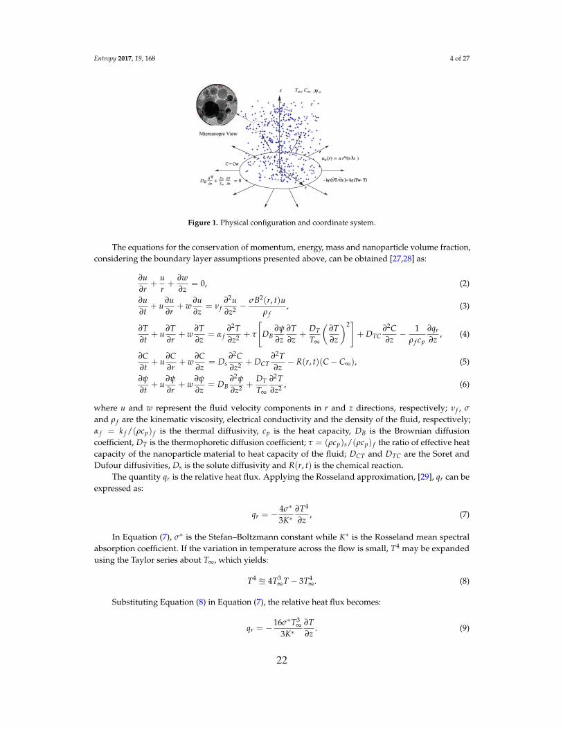
Consider the unsteady three-dimensional MHD flow of an incompressible viscous flow ofnanofluid. A cylindrical coordinate system (r, θ, z) is used. The velocity of the stretching sheetis assumed to be nonlinear along the radial direction. It is assumed that there is no nanoparticle fluxacross the wall, and the surface is stretching along the z-direction. In the ambient fluid, the temperature,solute concentration and nanoparticle concentration are denoted by T∞, C∞ and ψ∞, respectively(see Figure 1). Here, Cw, Tw and ψw represent the solute concentration, constant temperature andnanoparticle concentration respectively on the wall. The variable magnetic field intensity is denotedby B(r, t) where t represents time. The magnetic field acts in the positive z-direction normal to thesheet. In this study, B(r, t) generalizes the magnetic field term provided previously in [9,10] to:

B(r, t) =B0r(n−1)/2√

1− λt, (1)

where B0 is the uniform magnetic field strength, n > 0 is the power-law index or stretching sheetparameter and λ represents the unsteadiness parameter.

21

Entropy 2017, 19, 168 4 of 27

Figure 1. Physical configuration and coordinate system.

The equations for the conservation of momentum, energy, mass and nanoparticle volume fraction,considering the boundary layer assumptions presented above, can be obtained [27,28] as:

∂u∂r

+ur+

∂w∂z

= 0, (2)

∂u∂t

+ u∂u∂r

+ w∂u∂z

= ν f∂2u∂z2 −

σB2(r, t)uρ f

, (3)

∂T∂t

+ u∂T∂r

+ w∂T∂z

= α f∂2T∂z2 + τ

[DB

∂ψ

∂z∂T∂z

+DTT∞

(∂T∂z

)2]+ DTC

∂2C∂z− 1

ρ f cp

∂qr

∂z, (4)

∂C∂t

+ u∂C∂r

+ w∂C∂z

= Ds∂2C∂z2 + DCT

∂2T∂z− R(r, t)(C− C∞), (5)

∂ψ

∂t+ u

∂ψ

∂r+ w

∂ψ

∂z= DB

∂2ψ

∂z2 +DTT∞

∂2T∂z2 , (6)

where u and w represent the fluid velocity components in r and z directions, respectively; ν f , σ

and ρ f are the kinematic viscosity, electrical conductivity and the density of the fluid, respectively;α f = k f /(ρcp) f is the thermal diffusivity, cp is the heat capacity, DB is the Brownian diffusioncoefficient, DT is the thermophoretic diffusion coefficient; τ = (ρcp)s/(ρcp) f the ratio of effective heatcapacity of the nanoparticle material to heat capacity of the fluid; DCT and DTC are the Soret andDufour diffusivities, Ds is the solute diffusivity and R(r, t) is the chemical reaction.

The quantity qr is the relative heat flux. Applying the Rosseland approximation, [29], qr can beexpressed as:

qr = −4σ∗

3K∗∂T4

∂z, (7)

In Equation (7), σ∗ is the Stefan–Boltzmann constant while K∗ is the Rosseland mean spectralabsorption coefficient. If the variation in temperature across the flow is small, T4 may be expandedusing the Taylor series about T∞, which yields:

T4 u 4T3∞T − 3T4

∞. (8)

Substituting Equation (8) in Equation (7), the relative heat flux becomes:

qr = −16σ∗T3

∞3K∗

∂T∂z

. (9)

22

Entropy 2017, 19, 168 5 of 27

To simplify the mass equation, the chemical reaction R(r, t) must be a constant. This conditionholds if R(r, t) has the following form:

R(r, t) = R0arn−1

1− λt, (10)

where R0 is constant and a > 0 is the stretching constant.The boundary conditions considered (see [27]) are:

u = uw(r) =arn

1− λt, − k f

∂T∂z

= h f (Tw − T),

DB∂ψ

∂z+

DTT∞

∂T∂z

= 0, C = Cw at z = 0,

u→ 0, T → T∞, C → C∞ and

ψ→ ψ∞ as z→ ∞, (11)

where k f = k0√

1− λt is the thermal conductivity of the base fluid where k0 is a constant. A similaritysolution of the energy equation can be obtained if the Biot number,

Bi =h f

k0

√ν f

ar(n−1), (12)

is a constant. This condition is satisfied if the heat transfer coefficient, h f , is proportional to r(n−1)/2.Thus, the heat transfer coefficient is expressed as h f = b0r(n−1)/2, where b0 is a constant. The Biot

number can be obtained as Bi = h0

√(ν f /a)/k0.

Equations (2)–(6) are converted into coupled ordinary differential equations by using the followingsimilarity variables (see [27]):

η =

√a

ν f (1− λt)r(n−1)/2z, θ(η) =

T − T∞

Tw − T∞,

S(η) =C− C∞

Cw − C∞, φ(η) =

ψ− ψ∞

ψ∞. (13)

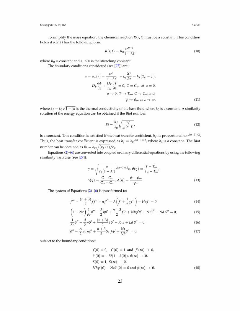
The system of Equations (2)–(6) is transformed to:

f ′′′ +(n + 3)

2f f ′′ − n f ′

2 − A(

f ′ +12

η f ′′)− Ha f ′ = 0, (14)

(1 + Nr

)1

Prθ′′ − A

2ηθ′ +

n + 32

f θ′ + Nbφ′θ′ + Ntθ′2+ Nd S′′ = 0, (15)

1Sc

S′′ − A2

ηS′ +(n + 3)

2f S′ − R0S + Ld θ′′ = 0, (16)

φ′′ − A2

Sc ηφ′ +n + 3

2Sc f φ′ +

NtNb

θ′′ = 0, (17)

subject to the boundary conditions:

f (0) = 0, f ′(0) = 1 and f ′(∞)→ 0,

θ′(0) = −Bi(1− θ(0)), θ(∞)→ 0,

S(0) = 1, S(∞)→ 0,

Nbφ′(0) + Ntθ′(0) = 0 and φ(∞)→ 0. (18)

23

Entropy 2017, 19, 168 6 of 27

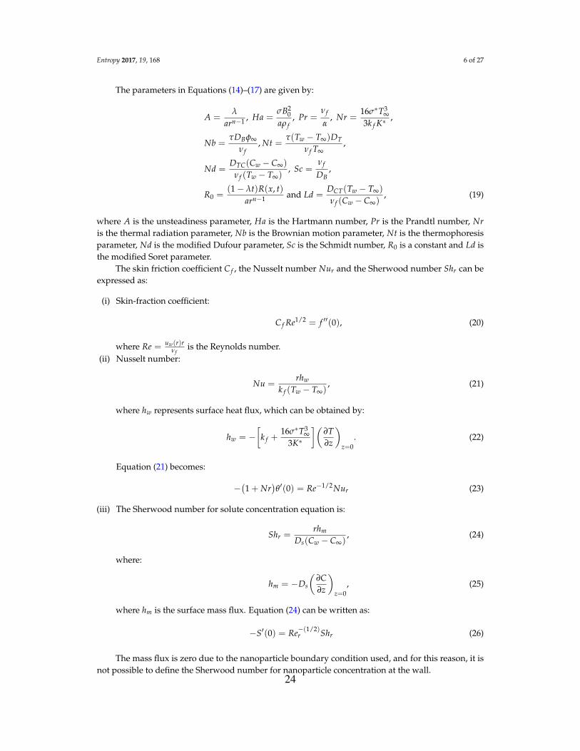
The parameters in Equations (14)–(17) are given by:

A =λ

arn−1 , Ha =σB2

0aρ f

, Pr =ν f

α, Nr =

16σ∗T3∞

3k f K∗,

Nb =τDBφ∞

ν f, Nt =

τ(Tw − T∞)DTν f T∞

,

Nd =DTC(Cw − C∞)

ν f (Tw − T∞), Sc =

ν f

DB,

R0 =(1− λt)R(x, t)

arn−1 and Ld =DCT(Tw − T∞)

ν f (Cw − C∞), (19)

where A is the unsteadiness parameter, Ha is the Hartmann number, Pr is the Prandtl number, Nris the thermal radiation parameter, Nb is the Brownian motion parameter, Nt is the thermophoresisparameter, Nd is the modified Dufour parameter, Sc is the Schmidt number, R0 is a constant and Ld isthe modified Soret parameter.

The skin friction coefficient C f , the Nusselt number Nur and the Sherwood number Shr can beexpressed as:

(i) Skin-fraction coefficient:

C f Re1/2 = f ′′(0), (20)

where Re = uw(r)rν f

is the Reynolds number.(ii) Nusselt number:

Nu =rhw

k f (Tw − T∞), (21)

where hw represents surface heat flux, which can be obtained by:

hw = −[

k f +16σ∗T3

∞3K∗

](∂T∂z

)

z=0. (22)

Equation (21) becomes:

−(1 + Nr

)θ′(0) = Re−1/2Nur (23)

(iii) The Sherwood number for solute concentration equation is:

Shr =rhm

Ds(Cw − C∞), (24)

where:

hm = −Ds

(∂C∂z

)

z=0, (25)

where hm is the surface mass flux. Equation (24) can be written as:

−S′(0) = Re−(1/2)r Shr (26)

The mass flux is zero due to the nanoparticle boundary condition used, and for this reason, it isnot possible to define the Sherwood number for nanoparticle concentration at the wall.

24

Entropy 2017, 19, 168 7 of 27

3. Entropy Generation Analysis

Entropy generation suggests a wastage of energy; thus, minimization of entropy production isoften a major objective. Entropy generation analysis can be used as an effective tool for the identificationof causes of inefficiency in any system and offers scope for the improvement in the design of any deviceor process. The limitation of global energy resources provides an impetus for re-examining energyproduction systems and consumption patterns (Arikoglu et al. [30]). From a theoretical perspective,the second law of thermodynamics is utilized to study energy producing, converting and consumingsystems. The volumetric rate of local entropy generation for a nanofluid along with thermal radiationand a magnetic field can be expressed as (see [18,22,23]:

Egen =k

T2∞

(( ∂T∂z

)2+

16σ∗T3∞

3K∗( ∂T

∂z

)2)

︸ ︷︷ ︸1st part

+µ

T∞

( ∂u∂z

)2

︸ ︷︷ ︸2nd part

+σB2

0

T∞u2

︸ ︷︷ ︸3rd part

+RDBψ∞

(∂ψ

∂z

)2

+RDB

T∞

( ∂T∂z

)( ∂ψ

∂z

)

︸ ︷︷ ︸4th part

(27)

In Equation (27), the entropy generation is stated in four parts. The first part is entropy generationdue to heat transfer irreversibility; the second part is the entropy generation due to the viscousdissipation irreversibility; the third part is the entropy generation due to the applied magnetic fieldirreversibility; and the fourth part is due to the diffusive irreversibility.

We define the entropy generation number as the ratio of the local volumetric entropy generationrate Egen to a characteristic rate of entropy generation E0, that is,

NG =Egen

E0, (28)

where:

E0 =k f (Tw − T∞)2

T2∞r2 . (29)

Using Equations (27)–(29), the non-dimensional entropy generation can be represented as:

NG = Re(1 + Nr

)θ′2(η) +

BrReΩ

f ′′2 +Br(

Ha)2

Ωf ′2

+ReΣΩ2 φ′2(η) +

ReΣΩ

θ′(η)φ′(η), (30)

where Re, Nr, Br, Ω, Ha, Σ are the Reynolds number, the thermal radiation parameter, Brinkmannumber, dimensionless temperature difference, Hartmann number and the diffusive parameter,respectively. These parameters are expressed by the following relations:

Br =µu2

w(r)k f ∆T

, Ω =∆TT∞

=Tw − T∞

T∞, Σ =

RDBψ∞

k f. (31)

4. Method of Solution

The quasi-linearization method (QLM) is a generalization of the Newton–Raphson method(Bellman and Kalaba [31]). The derivation of the QLM is based on the linearization of the nonlinearcomponents of the governing equations using the Taylor series assuming that the difference betweenthe value of the unknown function is negligible between the current iteration, r + 1, and the previousiteration, r.

25

Entropy 2017, 19, 168 8 of 27

Applying the quasi-linearization scheme to Equations (14)–(17) with the boundary conditions,Equation (18), yields the following iterative schemes:

a0,r f ′′′r+1 + a1,r f ′′r+1 + a2,r f ′r+1 + a3,r fr+1 = R f , (32)

b0,rθ′′r+1 + b1,rθ′r+1 + b2,rθr+1 + b3,r fr+1 + b4,rS′′r+1 + b5,rφ′r+1 = Rθ , (33)

c0,rS′′r+1 + c1,rS′r+1 + c2,rSr+1 + c3,r fr+1 + c4,rθ′′r+1 = RS, (34)

d0,rφ′′r+1 + d1,rφ′r+1 + d2,r fr+1 + d3,rθ′′r+1 = Rφ, (35)

subject to

fr+1(0) = 0, f ′r+1(0) = 1, f ′r+1(∞)→ 0,

θ′r+1(0) = −Bi(1− θr+1(0)), θr+1(∞)→ 0,

Sr+1(0) = 1, Sr+1(∞)→ 0,

Nbφ′r+1(0) + Ntθ′r+1(0) = 0, and φr+1(∞)→ 0, (36)

where the coefficients in Equations (32)–(35) are obtained as:

a0,r = 1, a1,r =

(n + 3

2

)fr −

A2

η,

a2,r = −2n f ′r − A− Ha, a3,r =

(n + 3

2

)f ′′r , (37)

b0,r =

(1 + Nr

)1

Pr,

b1,r =

(n + 3

2

)fr −

A2

η + Nbφ′r + 2Ntθ′r,

b2,r = 0, b3,r =

(n + 3

2

)θ′r,

b4,r = Nd, b5,r = Nbθ′r, (38)

c0,r =1Sc

, c1,r =

(n + 3

2

)fr −

A2

η, c2,r = −R0,

c3,r =

(n + 3

2

)S′r, c4,r = Ld, (39)

d0,r = 1, d1,r =

(n + 3

2

)Sc fr −

A2

Sc η,

d2,r =

(n + 3

2

)Sc φ′r, d3,r =

NtNb

. (40)

A Chebyshev pseudo-spectral method [24] was used to solve Equations (32)–(35). The Chebyshevinterpolating polynomial defined by Equation (41) is used with Gauss–Lobatto points [32,33] to definethe unknown functions where:

xi = cos(πi

N

), i = 0, 1, ..., N; −1 ≤ xi ≤ 1. (41)

The variable N in Equation (41) is the number of collocation points. A truncated domain [0, L] isused to approximate the semi-infinite domain to facilitate computations. The parameter L representsthe boundary condition at infinity. In order to model the behavior of the flow at infinity, the parameter Lshould be a large number. The domain [0, L] is transformed into [−1, 1] using the linear transformationη = L(x+1)

2 .

26

Entropy 2017, 19, 168 9 of 27

The spectral collocation method is used to construct a differentiation matrix to approximate thederivative of unknown variables at the collocation points as a matrix vector product:

dF(1)r

dη(ηj) =

N

∑k=0

Djk f (ηk) = DFm, j = 0, 1, 2, ..., N, (42)

where D = 2D/L and F =[

f (η0), f (η1), f (η1), ..., f (ηN)]T

represent the vector function at thecollocation points. The high order derivatives are given as powers of D, such as:

F(p)r = DpFr, (43)

where p is the order of the derivative. Spectral collocation is applied at r using the differentiation matrixD in order to approximate derivatives of unknown functions in Equations(32)–(35) with Equation (36),which yields:

A1,1f + A1,2θ+ A1,3S + A1,4φ = R f , (44)

A1,2f + A2,2θ+ A2,3S + A2,4φ = Rθ , (45)

A1,3f + A2,3θ+ A3,3S + A3,4φ = RS, (46)

A1,4f + A2,4θ+ A3,4S + A4,4φ = Rφ. (47)

Here:A1,1 = a0,rD3 + diag

(a1,r)D2 + diag

(a2,r)D + diag

(a3,r)I,

A1,2 = 0, A1,3 = 0, A1,4 = 0, (48)

A2,1 = diag(b3,1)I,

A2,2 = diag(b0,r)D2 + diag

(b1,r)D + diag

(b2,r)I, (49)

A2,3 = diag(b4,r)D2, A2,4 = diag

(b5,r)D,

A3,1 = diag(c3,r)I, A3,2 = diag

(c4,r)D2,

A3,3 = c0,rD2 + diag(c1,r)D +

(c2,r)I and (50)

A3,4 = 0,

A4,1 = diag(d2,r)I, A4,2 = diag

(d3,r)D2,

A4,3 = 0, A4,4 = diag(d0,r)D + diag

(d1,r)D, (51)

R f =

(n + 3

2

)frf′′r − n

(f′r)2, Rφ =

(n + 3

2

)Sc frφ

′r, (52)

Rs =

(n + 3

2

)frS′r and Rφ =

(n + 3

2

)Sc frφ

′r, (53)

where diag() represents diagonal matrices of order (N + 1)× (N + 1), I is an (N + 1)× (N + 1) identitymatrix and f, θ, S and φ are the values of functions f , θ, S and φ, respectively. Equations (44)–(47)are solved as a matrix system using the SQLM scheme where the iteration is started with initialapproximate solutions obtained as:

f0(η) = 1− exp(−η), θ0(η) =

(Bi

1 + Bi

)exp(−η),

S0(η) = exp(−η) and

φ0(η) = −(

NtNb

)(Bi

1 + Bi

)exp(−η). (54)

27

Entropy 2017, 19, 168 10 of 27

The above equations can be expressed in matrix form as follows:

A11 A12 A13 A14

A21 A22 A23 A24

A31 A32 A33 A34

A41 A42 A43 A44

Fr+1

Θr+1

Sr+1

Φr+1

=

R fRθ

Rs

Rφ

(55)

5. Results and Discussion

The study investigated entropy generation in an unsteady three-dimensional MHD nanofluidalong a nonlinear stretching sheet and considered the influence of thermal radiation and a chemicalreaction. The conservation equations are solved numerically using the spectral quasi-linearizationmethod (SQLM). The SQLM has been used in a limited number of studies to solve boundary layerflow, heat and mass transfer problems [34]. The physical parameters in this paper are mostly chosenfrom the literature, for example in the papers [21,26,27,35].

A comparison with previously published results is shown in Table 1 when A = 0, Ha = 0,Nr = 0, Nd = 0 and Ld = 0 (i.e., in the absence of unsteadiness parameter, Hartmann number,the thermal radiation number, Dufour parameter and Soret parameter, respectively). These results arecomparable to those of Mustafa et al. [27], which validates this numerical method.

Table 1. Current Nusselt number −θ′(0) compared with Mustafa et al. [27].

n Nt Sc Pr Mustafa et al. [27] Present Results

0.5 0.1 20 5 1.9112911 1.910680950.5 1.2170065 1.216590650.7 0.9815765 0.98122822

1.0 0.5 5 5 1.6914582 1.6910467510 1.4740787 1.4737517220 1.2861370 1.28590965

2.5 0.5 20 0.7 0.6619164 0.669866785 1.4784288 1.478477637 1.5758736 1.57604858

To demonstrate further the convergence of the SQLM, Figures 2–5 show the effect of the numberof collocation points on the accuracy of the solutions obtained for the velocity, temperature, soluteconcentration and nanoparticle concentration profiles, respectively.

0 50 100 150

Collocation points

10-10

10-8

10-6

10-4

10-2

100

102

||Res(f)|| ∞

SQLM

Figure 2. Effects of the number of collocation points number on the residual error of the velocityprofile ||Res( f )||∞ when n = 3, A = 0.3, Pr = 7, Ha = 0.5, Nr = 0.2, Nb = 0.5, Nt = 0.5, Nd = 0.02,Ld = 0.02, Sc = 7, R0 = 0.3, Bi = 0.2. 28

Entropy 2017, 19, 168 11 of 27

0 50 100 150

Collocation points

10-12

10-10

10-8

10-6

10-4

10-2

100

||Res(θ)|| ∞

SQLM

Figure 3. Effects of the number of collocation points number on the residual error of the temperatureprofile ||Res(θ)||∞ when n = 3, A = 0.3, Pr = 7, Ha = 0.5, Nr = 0.2, Nb = 0.5, Nt = 0.5, Nd = 0.02,Ld = 0.02, Sc = 7, R0 = 0.3, Bi = 0.2.

0 50 100 150

Collocation points

10-12

10-10

10-8

10-6

10-4

10-2

100

102

||Res(S

)|| ∞

SQLM

Figure 4. Effects of the number of collocation points number on the residual error of the soluteconcentration profile ||Res(S)||∞ when n = 3, A = 0.3, Pr = 7, Ha = 0.5, Nr = 0.2, Nb = 0.5,Nt = 0.5, Nd = 0.02, Ld = 0.02, Sc = 7, R0 = 0.3, Bi = 0.2.

0 50 100 150

Collocation points

10-12

10-10

10-8

10-6

10-4

10-2

100

102

||Res(φ)|| ∞

SQLM

Figure 5. Effects of the number of collocation points number on the residual error of the nanoparticleconcentration profile ||Res(φ)||∞ when n = 3, A = 0.3, Pr = 7, Ha = 0.5, Nr = 0.2, Nb = 0.5,Nt = 0.5, Nd = 0.02, Ld = 0.02, Sc = 7, R0 = 0.3, Bi = 0.2.

29

Entropy 2017, 19, 168 12 of 27

It was found that an increase in the number of collocation points results in a reduction of residualerror. However, after a certain point (the point at which an optimal residual error is obtained),an increase in the number of collocation points does not have a significant effect on residual error.

In Figure 2, it is observed that the optimal residual error for the velocity profile is around 10−9,which is achieved when the number of the collocation points is within the range 30 and 40; beyond thatrange, the accuracy starts declining. From Figures 3 and 5, it is noted that the optimal residual errorsfor the temperature and nanoparticle concentration profiles, respectively, are found around 10−12 whenthe number of collocation points is within 100 and 120. Figure 4 shows that the optimal residual of thesolute concentration profile occurs approximately at 10−11 when the number of collocation points isbetween 80 and 100. It is interesting to note that there is no magic number of collocation points thatinduces the optimal residual errors for all of the physical properties. Additionally, there is variability inthe behavior of the decline of the accuracy after the range at which the optimal residuals are obtained;for instance, in Figure 2, the accuracy of the solution of the velocity profile declines much fasteras compared to the accuracy of the solution of temperature, solute concentration and nanoparticleconcentration profiles respectively shown in Figures 3–5. Overall, these results demonstrate theaccuracy and convergence of the SQLM technique.

Table 2 shows the computed skin friction, heat transfer and the mass transfer coefficients, whichare represented by − f ′′(0), |−θ′(0)| and |−S′(0)|, respectively, for various values of n, A, Ha, Nr andPr. It is observed that the skin friction decreases as n increases, whereas the heat transfer coefficientand mass transfer increase with increasing n with other parameters fixed. It is also noted that the skinfriction reduces as A increases while the heat and mass transfer rates decrease. The skin friction, heatand mass transfer rates vary inversely with Ha and appear to be independent of changes in Nr, whilethe heat transfer rate decreases with the increase in Nr. The same result also holds for the skin frictionand the mass transfer with respect to Pr. The heat transfer increases when Pr increases.

Table 2. Skin friction coefficient, heat transfer coefficient and mass transfer coefficient for Nb = 0.5,Nt = 0.5, Nd = 0.02, Ld = 0.02, Sc = 7, R0 = 0.3, Bi = 0.2.

n A Ha Nr Pr − f ′′(0) −θ′(0) −S′(0)

1 1.43922866 −0.16417529 −2.891072572 0.3 0.5 0.2 7 1.70034047 −0.16661752 −3.169395934 2.12897896 −0.16969131 −3.66539915

−0.5 1.77701012 −0.17085800 −3.726864823 0 0.5 0.2 7 1.87092985 −0.16944779 −3.54329048

0.5 1.96353732 −0.16749470 −3.34434681

1.5 2.17151786 −0.16755905 −3.376067763 0.3 2.5 0.2 7 2.39114443 −0.16678981 −3.33136800

5 2.86708560 −0.16495200 −3.23526081

1 1.92657387 −0.16615306 −3.425332943 0.3 0.5 1.5 7 1.92657387 −0.16464481 −3.42514164

2 1.92657387 −0.16310964 −3.42504767

4 1.92657387 −0.16585371 −3.425534093 0.3 0.5 0.2 5 1.92657387 −0.16708464 −3.42554096

9 1.92657387 −0.16894896 −3.42668462

In Table 3 it is noted that for small values of the Biot number, small changes in the Biotnumber correspond to a large changes in the maximum temperature. In contrast, with high valuesof the Biot number, a large change in the Biot number does not appear to affect the maximumtemperature significantly.

30

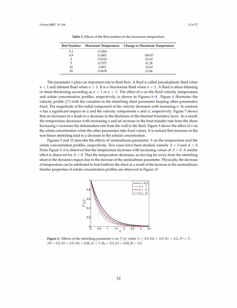
Entropy 2017, 19, 168 13 of 27

Table 3. Effects of the Biot number on the maximum temperature.

Biot Number Maximum Temperature Change in Maximum Temperature

0.1 0.12640.9 0.3401 169.072 0.5218 53.435 0.7377 41.38

10 0.853 15.6350 0.9678 13.46

The parameter n plays an important role in fluid flow. A fluid is called pseudoplastic fluid whenn < 1 and dilatant fluid when n > 1. It is a Newtonian fluid when n = 1. A fluid is shear-thinningor shear-thickening according as n < 1 or n > 1. The effect of n on the fluid velocity, temperatureand solute concentration profiles, respectively, is shown in Figures 6–8. Figure 6 illustrates thevelocity profile ( f ′) with the variation in the stretching sheet parameter keeping other parametersfixed. The magnitude of the radial component of the velocity decreases with increasing n. In contrast,n has a significant impact on η and the velocity components u and w, respectively. Figure 7 showsthat an increases in n leads to a decrease in the thickness of the thermal boundary layer. As a result,the temperature decreases with increasing n and an increase in the heat transfer rate from the sheet.Increasing n increases the deformation rate from the wall to the fluid. Figure 8 shows the effect of n onthe solute concentration when the other parameters take fixed values. It is noticed that increases in thenon-linear stretching lead to a decrease in the solutal concentration.

Figures 9 and 10 describe the effects of unsteadiness parameter A on the temperature and thesolute concentration profiles, respectively. Two cases have been studied, namely A < 0 and A > 0.From Figure 9, it is observed that the temperature increases with increasing values of A > 0. A similareffect is observed for A < 0. That the temperature decreases, as moving far away from the stretchingsheet in the dynamics region due to the increase of the unsteadiness parameter. Physically, the decreaseof temperature can be attributed to heat lostfrom the sheet as a result of the increase in the unsteadiness.Similar properties of solute concentration profiles are observed in Figure 10.

0 0.5 1 1.5 2 2.5 3 3.50

0.2

0.4

0.6

0.8

1

η

f′ (η)

n = 0.3

n = 1

n = 2

n = 4

Figure 6. Effects of the stretching parameter n on f ′(η) when A = 0.3, Ha = 0.5, Nr = 0.2, Pr = 7,Nb = 0.5, Nt = 0.5, Nd = 0.02, Sc = 7, R0 = 0.3, Ld = 0.02, Bi = 0.2.

31

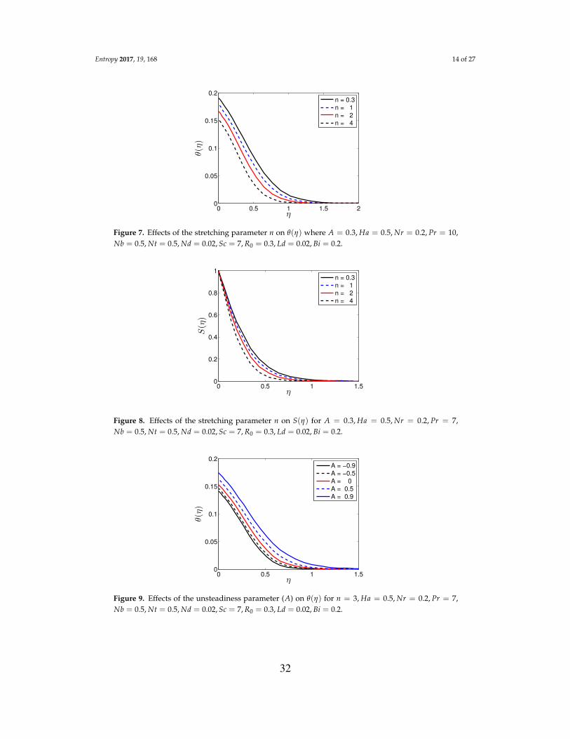
Entropy 2017, 19, 168 14 of 27

0 0.5 1 1.5 20

0.05

0.1

0.15

0.2

η

θ(η)

n = 0.3

n = 1

n = 2

n = 4

Figure 7. Effects of the stretching parameter n on θ(η) where A = 0.3, Ha = 0.5, Nr = 0.2, Pr = 10,Nb = 0.5, Nt = 0.5, Nd = 0.02, Sc = 7, R0 = 0.3, Ld = 0.02, Bi = 0.2.

0 0.5 1 1.50

0.2

0.4

0.6

0.8

1

η

S(η)

n = 0.3

n = 1

n = 2

n = 4

Figure 8. Effects of the stretching parameter n on S(η) for A = 0.3, Ha = 0.5, Nr = 0.2, Pr = 7,Nb = 0.5, Nt = 0.5, Nd = 0.02, Sc = 7, R0 = 0.3, Ld = 0.02, Bi = 0.2.

0 0.5 1 1.50

0.05

0.1

0.15

0.2

η

θ(η)

A = −0.9

A = −0.5

A = 0

A = 0.5

A = 0.9

Figure 9. Effects of the unsteadiness parameter (A) on θ(η) for n = 3, Ha = 0.5, Nr = 0.2, Pr = 7,Nb = 0.5, Nt = 0.5, Nd = 0.02, Sc = 7, R0 = 0.3, Ld = 0.02, Bi = 0.2.

32

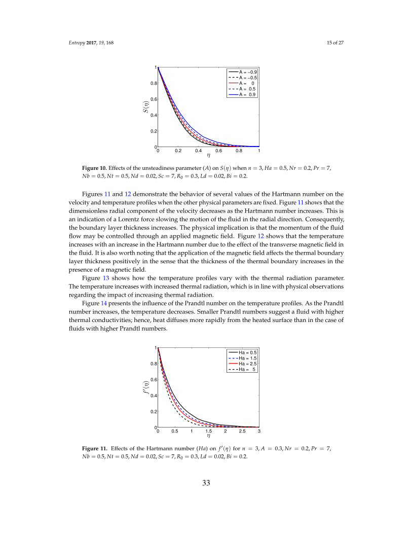
Entropy 2017, 19, 168 15 of 27

0 0.2 0.4 0.6 0.8 10

0.2

0.4

0.6

0.8

1

η

S(η)

A = −0.9

A = −0.5

A = 0

A = 0.5

A = 0.9

Figure 10. Effects of the unsteadiness parameter (A) on S(η) when n = 3, Ha = 0.5, Nr = 0.2, Pr = 7,Nb = 0.5, Nt = 0.5, Nd = 0.02, Sc = 7, R0 = 0.3, Ld = 0.02, Bi = 0.2.

Figures 11 and 12 demonstrate the behavior of several values of the Hartmann number on thevelocity and temperature profiles when the other physical parameters are fixed. Figure 11 shows that thedimensionless radial component of the velocity decreases as the Hartmann number increases. This isan indication of a Lorentz force slowing the motion of the fluid in the radial direction. Consequently,the boundary layer thickness increases. The physical implication is that the momentum of the fluidflow may be controlled through an applied magnetic field. Figure 12 shows that the temperatureincreases with an increase in the Hartmann number due to the effect of the transverse magnetic field inthe fluid. It is also worth noting that the application of the magnetic field affects the thermal boundarylayer thickness positively in the sense that the thickness of the thermal boundary increases in thepresence of a magnetic field.

Figure 13 shows how the temperature profiles vary with the thermal radiation parameter.The temperature increases with increased thermal radiation, which is in line with physical observationsregarding the impact of increasing thermal radiation.

Figure 14 presents the influence of the Prandtl number on the temperature profiles. As the Prandtlnumber increases, the temperature decreases. Smaller Prandtl numbers suggest a fluid with higherthermal conductivities; hence, heat diffuses more rapidly from the heated surface than in the case offluids with higher Prandtl numbers.

0 0.5 1 1.5 2 2.5 30

0.2

0.4

0.6

0.8

1

η

f′ (η)

Ha = 0.5

Ha = 1.5

Ha = 2.5

Ha = 5

Figure 11. Effects of the Hartmann number (Ha) on f ′(η) for n = 3, A = 0.3, Nr = 0.2, Pr = 7,Nb = 0.5, Nt = 0.5, Nd = 0.02, Sc = 7, R0 = 0.3, Ld = 0.02, Bi = 0.2.

33

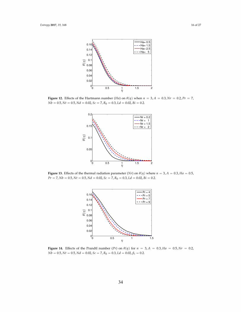
Entropy 2017, 19, 168 16 of 27

0 0.5 1 1.5 20

0.02

0.04

0.06

0.08

0.1

0.12

0.14

0.16

η

θ(η)

Ha= 0.5

Ha= 1.5

Ha= 2.5

Ha= 5

Figure 12. Effects of the Hartmann number (Ha) on θ(η) when n = 3, A = 0.3, Nr = 0.2, Pr = 7,Nb = 0.5, Nt = 0.5, Nd = 0.02, Sc = 7, R0 = 0.3, Ld = 0.02, Bi = 0.2.

0 0.5 1 1.5 20

0.05

0.1

0.15

0.2

η

θ(η)

Nr = 0.2

Nr = 1

Nr = 1.5

Nr = 2

Figure 13. Effects of the thermal radiation parameter (Nr) on θ(η) where n = 3, A = 0.3, Ha = 0.5,Pr = 7, Nb = 0.5, Nt = 0.5, Nd = 0.02, Sc = 7, R0 = 0.3, Ld = 0.02, Bi = 0.2.

0 0.5 1 1.50

0.02

0.04

0.06

0.08

0.1

0.12

0.14

0.16

η

θ(η)

Pr = 4

Pr = 5

Pr = 7

Pr = 9

Figure 14. Effects of the Prandtl number (Pr) on θ(η) for n = 3, A = 0.3, Ha = 0.5, Nr = 0.2,Nb = 0.5, Nt = 0.5, Nd = 0.02, Sc = 7, R0 = 0.3, Ld = 0.02, βi = 0.2.

34

Entropy 2017, 19, 168 17 of 27

Figure 15 illustrates the behavior of the temperature profiles with different values of thethermophoresis parameter, Nt, when the other parameter are fixed. It is observed that the temperatureincreases as the thermophoresis parameter increases because the thermal boundary layer increaseswith increases in the thermophoresis parameter.

0 0.5 1 1.50

0.02

0.04

0.06

0.08

0.1

0.12

η

θ(η)

Nt = 0.5

Nt = 1.5

Nt = 2

Nt = 2.5

Figure 15. Effects of the thermophoresis parameter (Nt) on θ(η) for n = 3, A = 0.3, Ha = 0.5, Nr = 0.2,Pr = 7, Nb = 0.5, Nd = 0.02, Sc = 7, R0 = 0.3, Ld = 0.02, Bi = 0.2.

Figure 16 demonstrates the influence of the Schmidt number on the solute concentration profilewith fixing the other parameters. It is noticed that the solute concentration decreases as the Schmidtnumber increases.

0 0.5 1 1.50

0.2

0.4

0.6

0.8

1

η

S(η)

Sc = 4

Sc = 5

Sc = 7

Sc = 9

Figure 16. Effects of the Schmidt number (Sc) on S(η) for n = 3, A = 0.3, Ha = 0.5, Nr = 0.2,Pr = 7, Nb = 0.5, Nt = 0.5, R0 = 0.3, Bi = 0.2.

Figure 17 shows the relation between the Biot number Bi and the temperature profiles. The Biotnumber can be perceived as the ratio of internal (conductive) resistance of solid to external (convectiveresistance). Here, it is found that temperature increases with the increase in the Biot number. An increasein the Biot number causes a stronger convection, and this leads to higher surface temperatures. Further,for sufficiently large values of the Biot number, the temperature approaches its maximum value.

35

Entropy 2017, 19, 168 18 of 27

0 0.5 1 1.50

0.2

0.4

0.6

0.8

1

ηθ(η)

Bi= 0.1

Bi= 0.9

Bi= 2

Bi= 5

Bi= 10

Bi= 50

Figure 17. Effects of the Biot number (Bi) on θ(η) for n = 3, A = 0.3, Ha = 0.5, Nr = 0.2, Pr = 7,Nb = 0.5, Nt = 0.5, Nd = 0.02, Sc = 7, R0 = 0.3, Ld = 0.02.

Figure 18 shows that high values of the stretching sheet parameter n lead to a reduction in thethickness of the nanoparticle concentration boundary layer thickness up to a certain value of η. Beyondthis critical distance, the opposite trend is observed. In Figure 19, we observe a similar pattern ofnanoparticle concentration profiles as in Figures 9 and 10. In Figure 20, the nanoparticle concentrationprofiles increase with the thermophoresis parameter. Similar results are shown in Figure 21 for theBrownian motion parameter. In Figure 22, it is observed that increasing the Schmidt number reducesthe nanoparticle concentration profile. The Schmidt number Sc has an opposite effect on the Browniandiffusion coefficient. When DB is small, the penetration depth of the nanoparticle concentrationprofiles becomes shorter. Thus, as the Schmidt number increases, the penetration depth becomesshorter. Moreover, the increase in Sc results in a decrease in the concentration rate, as well as the heattransfer rate.

It is interesting to note that Figures 23–27 suggest different ways of controlling the entropygeneration. Figure 23 shows the effect of the Reynolds number on the entropy generation NG. It isobserved that entropy generation increases with the increase in the Reynolds number. This observationcould be explained by the increase in random eddies, vortices and flow fluctuation in the fluid, whichare associated with increasing Re. As a consequence, the heat transfer increases, which, in turn,enhances the entropy generation. The entropy generation number increases in the proximity of thesheet due to a decrease in the fluid friction. Reducing the Reynolds number induces a reduction in theentropy generation number.

0 0.5 1 1.5 2 2.50

0.005

0.01

0.015

0.02

0.025

0.03

η

φ(η)

n = 0.3

n = 1

n = 2

n = 4

Figure 18. Effects of the stretching parameter (n) on φ(η) when A = 0.3, Ha = 0.5, Nr = 0.2, Pr = 7,Nb = 0.5, Nt = 0.5, Nd = 0.02, Sc = 7, R0 = 0.3, Ld = 0.02, Bi = 0.2.

36

Entropy 2017, 19, 168 19 of 27

0 0.5 1 1.5 2 2.50

0.005

0.01

0.015

0.02

0.025

0.03

0.035

η

φ(η)

A = −0.9

A = −0.5

A = 0

A = 0.5

A = 0.9

Figure 19. Effects of the unsteadiness parameter (A) on φ(η) for n = 3, Ha = 0.5, Nr = 0.2, Pr = 7,Nb = 0.5, Nt = 0.5, Nd = 0.02, Sc = 7, R0 = 0.3, Ld = 0.02, Bi = 0.2.

0 0.5 1 1.50

0.01

0.02

0.03

0.04

0.05

0.06

0.07

0.08

η

φ(η)

Nt = 0.5

Nt = 1.5

Nt = 2

Nt = 2.5

Figure 20. Effects of the thermophoresis parameter (Nt) on φ(η) for n = 3, A = 0.3, Ha = 0.5,Nr = 0.2, Pr = 7, Nb = 0.5, Nd = 0.02, Sc = 7, R0 = 0.3, Ld = 0.02, Bi = 0.2.

0 0.5 1 1.50

0.005

0.01

0.015

0.02

0.025

η

φ(η)

Nb = 0.5

Nb = 1

Nb = 1.5

Nb = 2

Figure 21. Effects of the Brownian motion parameter (Nb) on φ(η) when n = 3, A = 0.3, Ha = 0.5,Nr = 0.2, Pr = 7, Nt = 0.5, Nd = 0.02, Sc = 7, R0 = 0.3, Ld = 0.02, Bi = 0.2.

37

Entropy 2017, 19, 168 20 of 27

0 0.5 1 1.5 2 2.5 3 3.50

0.005

0.01

0.015

0.02

0.025

0.03

η

φ(η)

Sc = 4

Sc = 5

Sc = 7

Sc = 9

Figure 22. Effects of the Schmidt number (Sc) on φ(η) for n = 3, A = 0.3, Ha = 0.5, Nr = 0.2,Pr = 7, Nb = 0.5, Nt = 0.5, R0 = 0.3, Bi = 0.2.

0 0.5 1 1.50

2

4

6

8

10

η

NG

Re = 0.5

Re = 1.2

Re = 2

Re = 2.5

Figure 23. Effects of the Reynolds number Re on the entropy generation number NG when Nr = 0.2,Br = 1, Ω = 1, Ha = 0.5 and Σ = 0.5.

0 0.5 1 1.50

5

10

15

20

η

NG

Br = 0.5

Br = 1.2

Br = 2

Br = 2.5

Figure 24. Effects of Brinkman number Br on the entropy generation number NG when Re = 2,Nr = 0.2, Ω = 1, Ha = 0.5 and Σ = 0.5.

38

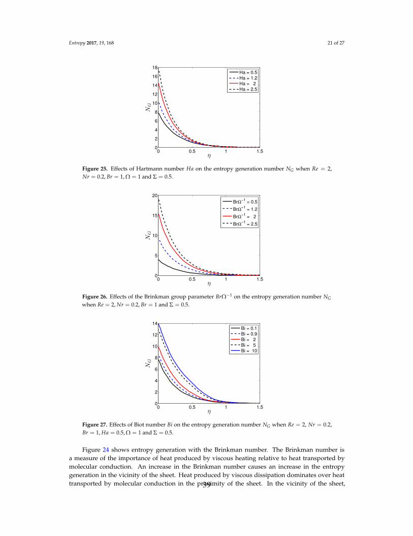
Entropy 2017, 19, 168 21 of 27

0 0.5 1 1.50

2

4

6

8

10

12

14

16

18

ηN

G

Ha = 0.5

Ha = 1.2

Ha = 2

Ha = 2.5

Figure 25. Effects of Hartmann number Ha on the entropy generation number NG when Re = 2,Nr = 0.2, Br = 1, Ω = 1 and Σ = 0.5.

0 0.5 1 1.50

5

10

15

20

η

NG

BrΩ−1

= 0.5

BrΩ−1

= 1.2

BrΩ−1

= 2

BrΩ−1

= 2.5

Figure 26. Effects of the Brinkman group parameter BrΩ−1 on the entropy generation number NG

when Re = 2, Nr = 0.2, Br = 1 and Σ = 0.5.

0 0.5 1 1.50

2

4

6

8

10

12

14

η

NG

Bi = 0.1

Bi = 0.9

Bi = 2

Bi = 5

Bi = 10

Figure 27. Effects of Biot number Bi on the entropy generation number NG when Re = 2, Nr = 0.2,Br = 1, Ha = 0.5, Ω = 1 and Σ = 0.5.

Figure 24 shows entropy generation with the Brinkman number. The Brinkman number isa measure of the importance of heat produced by viscous heating relative to heat transported bymolecular conduction. An increase in the Brinkman number causes an increase in the entropygeneration in the vicinity of the sheet. Heat produced by viscous dissipation dominates over heattransported by molecular conduction in the proximity of the sheet. In the vicinity of the sheet,39

Entropy 2017, 19, 168 22 of 27

significant heat generation occurs within the layers of the moving fluid particles, which in turn increasesthe entropy generation number by enhancing the degree of disorder of the system. This graduallyfades with the distance from the sheet.

The influence of the Hartmann number on the entropy generation number is given in Figure 25.In close proximity to the sheet, an increase in the Hartmann number corresponds to a noticeableincrease in the entropy generation, whereas far from the sheet, the increase in the Hartmann numberhas rather negligible impact on entropy generation. This change in entropy generation number inresponse to the Hartmann number is related to the increase in the resistance of the fluid motion due toan increase in the Hartmann number. This variation in entropy generation with the Hartmann numbercan be attributed to higher heat transfer rates, which result in an increase of the entropy generationnumber. However, far from the sheet, the effect of the Hartmann number is insignificant, causing acorresponding insignificant entropy generation.

Figure 26 displays the entropy generation with the Brinkman parameter (BrΩ−1). An increase inBrΩ−1 results in a remarkable increase in the entropy generation number in the area surrounding thesheet. The increase in the entropy generation number around the sheet due to the increase in BrΩ−1

can be related to a decrease in the fluid friction caused by increasing BrΩ−1. Moreover, Equation (31)suggests that the increase in BrΩ−1 results in an increase in the sheet velocity, which affects the fluidin the surroundings of the sheet and that explains, in part, the noticeable effect of BrΩ−1 on theentropy generation proximity of the sheet and the negligible effect in the further region. Figure 27demonstrates the relation between the Biot number and the entropy generation number. The entropygeneration number increases prominently in the proximity of the sheet as the Biot number increases.On the contrary, the Biot number has an insignificant effect on the entropy generation number far awayfrom the sheet.

Figure 28 demonstrates how the skin friction − f ′′(0) varies according to different values of themagnetic field parameter Ha and the stretching sheet parameter n. It is observed that − f ′′(0) increaseswith increasing values of Ha and n.

0 0.5 1 1.5 2 2.5

Ha

1

1.2

1.4

1.6

1.8

2

2.2

2.4

−f′′(0)

n = 0.5

n = 1

n = 1.5

n = 2

Figure 28. Effect of the magnetic field Ha and the stretching sheet parameter n on the skin friction− f ′′(0) when A = 0.3, Pr = 7, Nr = 0.2, Nb = 0.5, Nt = 0.5, Nd = 0.02, Ld = 0.02, Sc = 7, R0 = 0.3,Bi = 0.2.

The variation in the Nusselt number −θ′(0) due to the thermophoresis number Nt and thestretching sheet parameter n is graphed in Figure 29. It is noticed that with increasing values of Ntand n, −θ′(0) decreases.

Figure 30 displays the change in the Sherwood number −S′(0) caused by the effect of the Schmidtnumber Sc and the stretching sheet parameter n. It is observed that −S′(0) increases as Sc andn increase.

40

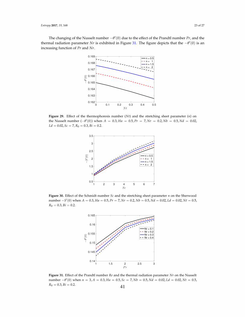
Entropy 2017, 19, 168 23 of 27

The changing of the Nusselt number −θ′(0) due to the effect of the Prandtl number Pr, and thethermal radiation parameter Nr is exhibited in Figure 31. The figure depicts that the −θ′(0) is anincreasing function of Pr and Nr.

0 0.1 0.2 0.3 0.4 0.5

Nt

0.162

0.163

0.164

0.165

0.166

0.167

0.168

0.169

−θ′ (0)

n = 0.5

n = 1

n = 1.5

n = 2

Figure 29. Effect of the thermophoresis number (Nt) and the stretching sheet parameter (n) onthe Nusselt number (−θ′(0)) when A = 0.3, Ha = 0.5, Pr = 7, Nr = 0.2, Nb = 0.5, Nd = 0.02,Ld = 0.02, Sc = 7, R0 = 0.3, Bi = 0.2.

1 2 3 4 5 6 7

Sc

0.5

1

1.5

2

2.5

3

3.5

−S′ (0)

n = 0.5

n = 1

n = 1.5

n = 2

Figure 30. Effect of the Schmidt number Sc and the stretching sheet parameter n on the Sherwoodnumber −S′(0) when A = 0.3, Ha = 0.5, Pr = 7, Nr = 0.2, Nb = 0.5, Nd = 0.02, Ld = 0.02, Nt = 0.5,R0 = 0.3, Bi = 0.2.

1 1.5 2 2.5 3

Pr

0.14

0.145

0.15

0.155

0.16

0.165

−θ′ (0)

Nr = 0.1

Nr = 0.2

Nr = 0.3

Nr = 0.4

Figure 31. Effect of the Prandtl number Re and the thermal radiation parameter Nr on the Nusseltnumber −θ′(0) when n = 3, A = 0.3, Ha = 0.5, Sc = 7, Nb = 0.5, Nd = 0.02, Ld = 0.02, Nt = 0.5,R0 = 0.3, Bi = 0.2. 41

Entropy 2017, 19, 168 24 of 27

6. Conclusions

A mathematical formulation and analysis of the entropy generation rate in an unsteadythree-dimensional axisymmetric MHD nanofluid flow over a non-linear stretching sheet subjectto thermal radiation and a chemical reaction has been presented. The influence of different physicalparameters on the entropy generation number has been demonstrated and discussed in detail. Fromthe discussion, the following outcomes may be inferred:

1. The heat transfer rate increases with increasing sheet stretching.2. An increase in the Reynolds number and the Brinkman number corresponds to a significant

increase in the entropy generation number. Therefore, it can be ascertained that the entropygeneration number is highly affected by viscous dissipation when the nanofluid flow has a largeReynolds number.

3. An increase in the Biot and Hartmann numbers corresponds to a significant increase in the entropygeneration number in the vicinity of the sheet surface. The significance of the Biot and Hartmannnumbers gradually fades with distance from the sheet.

4. The entropy generation rate can be minimized by controlling the physical parameters.5. The number of collocation points has a significant influence on the accuracy of the solutions.

Acknowledgments: The authors would like to thank the University of KwaZulu-Natal, DST-NRF Centre ofExcellence in Mathematical and Statistical Sciences (CoE-MaSS) and Claude Leon Foundation, South Africa, forthe financial support. Furthermore, the authors are thankful to the reviewers for their valuable comments andsuggestions, which have improved the quality of this paper.

Author Contributions: Sabyasachi Mondal proposed the main idea and design framework. Mohammed Almakkicarried out the numerical simulations and the first draft of this paper. Sharadia Dey and Precious Sibanda revisedthe draft, done some write-up and checked the calculations. All authors contributed equally in the analysis ofthe results.

Conflicts of Interest: The authors declare no conflict of interest.

Abbreviations

The following abbreviations are used in this manuscript:

r, θ, z cylindrical polar coordinate axesB0 magnetic field strength (kg·s−2A−1)u velocity in radial direction (m·s−1)n, λ constantsw velocity in axial direction (m·s−1)ν f kinematic viscosity (m2s−1)T temperature variable (K)σ electrical conductivity (Ω−1m−1)Tw temperature of fluid at sheet (K)ρ f density of fluid (kg·m−3)T∞ ambient temperature of fluid (K)α f thermal diffusion of fluid (m2s−1)C solute concentration of fluid (kg·m−3)CW solute concentration at wall (kg·m−3)C∞ solute concentration far away from the disk (kg·m−3)ψ nanoparticle concentrationψW nanoparticle concentration at wallψ∞ nanoparticle concentration far away from the disk

42

Entropy 2017, 19, 168 25 of 27

τ ratio of nanoparticle heat capacityDB Brownian mention coefficient (kg·m−1s−1)DT Thermophoretic diffusion coefficient (kg·m−1s−1K−1)DTC Dufour diffusion coefficientcp specific heat (m2s−2K−1)k f thermal conductivity (W·m−1K−1)qr radiative heat flux (kg·m−2)Ds solute diffusion coefficientDCT Soret diffusion coefficientR chemical reaction parameter(ρcp)s heat capacity of the nanoparticle(ρcp) f heat capacity of fluidσ∗ Stefan–Boltzmann constantK∗ mean absorption coefficientR0, a constantsk0, b0 constantsh f heat transfer coefficient (W·m−2 K−1)Bi Biot numberη dimensionless variableθ dimensionless temperatureS dimensionless solute concentrationφ dimensionless nanoparticle concentrationf dimensionless velocityA unsteadiness parameterHa Hartmann numberNr thermal radiation parameterPr Prandtl numberNb Brownian mention parameterNt Thermophoresis parameterNd Dufour parameterSc Schmidt numberLd Soret parameterC f skin friction coefficientNur Nusselt numberShr Sherwood numberuw(r) velocity of the stretching sheetRe Reynolds numberhw heat flux (W·m−2)hm mass flux (kg·m−2s−1)Egen volumetric entropy generation per unit length (W·m−3 K−1)E0 dimensionless entropy generation rateBr Brinkman numberΩ dimensionless parameterHa Hartmann numberΣ diffusive constant parameter∆T difference between (TW − T∞)(K)

References

1. Dessie, H.; Kishan, N. Unsteady MHD flow of heat and mass transfer of nanofluids over stretching sheetwith a non-uniform heat/source/sink considering viscous dissipation and chemical reaction. Int. J. Eng.Res. Afr. 2015, 14, doi:10.4028/www.scientific.net/JERA.14.1.

2. Chol, S. Enhancing thermal conductivity of fluids with nanoparticles. ASME Publ. FED 1995, 231, 99–106.3. Buongiorno, J. Convective transport in nanofluids. J. Heat Transf. 2006, 128, 240–250.

43

Entropy 2017, 19, 168 26 of 27

4. Ahmed, N.; Goswami, J.; Barua, D. Effects of chemical reaction and radiation on an unsteady MHD flow pastan accelerated infinite vertical plate with variable temperature and mass transfer. Indian J. Pure Appl. Math.2013, 44, 443–466.

5. Ahmed, J.; Mahmood, T.; Iqbal, Z.; Shahzad, A.; Ali, R. Axisymmetric flow and heat transfer over anunsteady stretching sheet in power law fluid. J. Mol. Liq. 2016, 221, 386–393.

6. Mohammadiun, H.; Rahimi, A.; Kianifar, A. Axisymmetric stagnation-point flow and heat transfer of aviscous, compressible fluid on a cylinder with constant heat flux. Sci. Iran. 2013, 20, 185–194.

7. Xiao, B.; Yang, Y.; Chen, L. Developing a novel form of thermal conductivity of nanofluids with Brownianmotion effect by means of fractal geometry. Powder Technol. 2013, 239, 409–414.

8. Cai, J.; Hu, X.; Xiao, B.; Zhou, Y.; Wei, W. Recent developments on fractal-based approaches to nanofluidsand nanoparticle aggregation. Int. J. Heat Mass Transf. 2017, 105, 623–637.

9. Shankar, B.; Yirga, Y. Unsteady heat and mass transfer in MHD flow of nanofluids over stretching sheet witha non-uniform heat source/sink. Int. J. Math. Comput. Sci. Eng. 2013, 7, 1267–1275.

10. Shahzad, A.; Ali, R.; Khan, M. On the exact solution for axisymmetric flow and heat transfer over a nonlinearradially stretching sheet. Chin. Phys. Lett. 2012, 29, 084705.

11. Ahmad, S.; Ashraf, M.; Syed, K. Effects of thermal radiation on MHD axisymmetric stagnation point flowand heat transfer of a micropolar fluid over a shrinking sheet. World Appl. Sci. J. 2011, 15, 835–848.

12. Mabood, F.; Shafiq, A.; Hayat, T.; Abelman, S. Radiation effects on stagnation point flow with melting heattransfer and second order slip. Results Phys. 2017, 7, 31–42.

13. Prasad, K.; Vaidya, H.; Vajravelu, K.; Datti, P.; Umesh, V. Axisymmetric mixed convective MHD flow over aslender cylinder in the presence of chemically reaction. Int. J. Appl. Mech. Eng. 2016, 21, 121–141.

14. Sarada, K.; Shanker, B. The effect of chemical reaction on an unsteady MHD free convection flow past aninfinite vertical porous plate with variable suction. Int. J. Eng. Mod. Res. 2013, 3, 725–735.

15. Hunegnaw, A.; Kishan, N. Unsteady MHD heat and mass transfer flow over stretching sheet in porousmedium with variable properties considering viscous dissipation and chemical reaction. Am. Chem. Sci. J.2014, 4, 901–917.

16. Barik, R. Heat and Mass Transfer Effects on Unsteady MHD Flow through an Accelerated Isothermal VerticalPlate Embedded in Porous Medium in the Presence of Heat Source and Chemical Reaction. Eur. J. Adv.Eng. Technol. 2016, 3, 56–61.

17. Bejan, A. Entropy Generation Minimization: The Method of Thermodynamic Optimization of Finite-Size Systemsand Finite-Time Processes; CRC Press: Boca Raton, FL, USA, 1995.

18. Qing, J.; Bhatti, M.M.; Abbas, M.A.; Rashidi, M.M.; Ali, M.E.S. Entropy generation on MHD Casson nanofluidflow over a porous stretching/shrinking surface. Entropy 2016, 18, 123.

19. Rashidi, M.M.; Bhatti, M.M.; Abbas, M.A.; Ali, M.E.S. Entropy generation on MHD blood flow of nanofluiddue to peristaltic waves. Entropy 2016, 18, 117.

20. Bhatti, M.M.; Abbas, T.; Rashidi, M.M.; Ali, M.E.S.; Yang, Z. Entropy generation on MHD eyring—Powellnanofluid through a permeable stretching surface. Entropy 2016, 18, 224.

21. Rashidi, M.; Mohammadi, F.; Abbasbandy, S.; Alhuthali, M. Entropy generation analysis for stagnation pointflow in a porous medium over a permeable stretching surface. J. Appl. Fluid Mech. 2015, 8, 753–765.

22. Bhatti, M.M.; Abbas, T.; Rashidi, M.M.; Ali, M.E.S. Numerical simulation of entropy generation with thermalradiation on MHD Carreau nanofluid towards a shrinking sheet. Entropy 2016, 18, 200.

23. Freidoonimehr, N.; Rahimi, A.B. Comment on “Effects of thermophoresis and Brownian motion on nanofluidheat transfer and entropy generation” by M. Mahmoodi, Sh. Kandelousi, Journal of Molecular Liquids,211 (2015) 15–24. J. Mol. Liq. 2016, 216, 99–102.

24. Agbaje, T.; Mondal, S.; Makukula, Z.; Motsa, S.; Sibanda, P. A new numerical approach to MHD stagnationpoint flow and heat transfer towards a stretching sheet. Ain Shams Eng. J. 2016, in press.

25. Kaladhar, K.; Motsa, S.; Srinivasacharya, D. Mixed Convection Flow of Couple Stress Fluid in a VerticalChannel with Radiation and Soret Effects. J. Appl. Fluid Mech. 2016, 9, 43–50.

26. Nield, D.; Kuznetsov, A. The onset of convection in a horizontal nanofluid layer of finite depth: A revisedmodel. Int. J. Heat Mass Transf. 2014, 77, 915–918.

27. Mustafa, M.; Khan, J.A.; Hayat, T.; Alsaedi, A. Analytical and numerical solutions for axisymmetric flow ofnanofluid due to non-linearly stretching sheet. Int. J. Non Linear Mech. 2015, 71, 22–29.

44

Entropy 2017, 19, 168 27 of 27

28. Sajid, M.; Hayat, T.; Asghar, S.; Vajravelu, K. Analytic solution for axisymmetric flow over a nonlinearlystretching sheet. Arch. Appl. Mech. 2008, 78, 127–134.

29. Pal, D. Heat and mass transfer in stagnation-point flow towards a stretching surface in the presence ofbuoyancy force and thermal radiation. Meccanica 2009, 44, 145–158.

30. Arikoglu, A.; Ozkol, I.; Komurgoz, G. Effect of slip on entropy generation in a single rotating disk in MHDflow. Appl. Energy 2008, 85, 1225–1236.

31. Bellman, R.E.; Kalaba, R.E. Quasilinearization and Nonlinear Boundary-Value Problems; RAND Corporation:New York, NY, USA, 1965.

32. Canuto, C.; Hussaini, M.Y.; Quarteroni, A.M.; Thomas, A., Jr. Spectral Methods in Fluid Dynamics; Springer:Berlin/Heidelberg, Germany, 2012.

33. Trefethen, L.N. Spectral Methods in MATLAB; SIAM: Oxford, UK, 2000.34. Motsa, S.; Sibanda, P.; Shateyi, S. On a new quasi-linearization method for systems of nonlinear boundary

value problems. Math. Methods Appl. Sci. 2011, 34, 1406–1413.35. Rashidi, M.; Abelman, S.; Mehr, N.F. Entropy generation in steady MHD flow due to a rotating porous disk

in a nanofluid. Int. J. Heat Mass Transf. 2013, 62, 515–525.

c© 2017 by the authors. Licensee MDPI, Basel, Switzerland. This article is an open accessarticle distributed under the terms and conditions of the Creative Commons Attribution(CC BY) license (http://creativecommons.org/licenses/by/4.0/).

45

Chapter 3

Entropy generation in unsteady MHD microp-

olar nanofluid flow with viscous dissipation

and thermal radiation

In Chapter 2, we studied the entropy generation in Newtonian fluid flow which is described by

a system of ordinary differential equations. Despite being more complex than Newtonian fluids,

non-Newtonian fluids have significantly more uses in industry. This chapter extends the work in

Chapter 2 to a non-Newtonian fluid flow which is described by partial differential equations.

In this chapter we consider entropy generation in unsteady two-dimensional magneto-micropolar

nanofluid flow along a linear stretching sheet in a porous medium with heat generation and a

chemical reaction. The flow is subject to viscous dissipation and thermal radiation. Thermophoesis

and nanoparticle Brownian motion are taken into account. The bivariate spectral quasiliearization

method is used solve the model equations.

46

Entropy generation in unsteady magneto-micropolar nanofluid flowwith viscous dissipation and thermal radiation

M. Almakki, H.Mondal∗and P. SibandaSchool of Mathematics, Statistics and Computer Science University of KwaZulu-Natal

Pietermaritzburg Private Bag X01Scottsville 3209, South Africa

August 28, 2018

AbstractWe investigate entropy generation in magneto-micropolar nanofluid flow, particle deposition and

thermal radiation effects on boundary layer flow over a stretching sheet with heat generation and achemical reaction. A novel feature of this study is the investigation of entropy generation in a combinedmicropolar nanofluid and the use of the recently developed bivariate spectral quasiliearization method tosolve the conservation equations. It is found that the method converges fast and accurate results can beachieved with this new method. The results show that entropy generation can be controlled to a degreeby controlling the Brinkman and Reynold number.

Keyword: Micropolar, Nanofluids; Entropy generation; Thermal radiation; viscous dissipation

1 IntroductionThe MHD micropolar nanofluid flow with a stretching surface has gained increasing importance duringrecent years owing to the great variety of applications it has on engineering and geophysics. The non-Newtonian fluids help us to understand the behaviour of a wide variety of fluids including micropolar fluids.The viscosity is mainly used to characterize the thickness of a fluid, its behaviors like of non-Newtonianfluids. The micropolar fluids are regarded as isotropic-polar fluids with negligence of the deformation ofmolecules. Physically, this model can capture the independent rotation of the molecules of the fluids and thelocal vorticity. A fluid represented by such a model can exhibit body couples, couple stresses, and exhibitmicrorotational and microinertial effects. This occurs in thermal energy storage, aerodynamic extrusion ofpolymer sheets, petroleum reservoirs. Magneto-micropolar fluids can be used to model body fluids includingcerebral-spinal fluid. Hassanien et al. [1] investigated the micropolar fluid flow along a non-isothermalstretching sheet with suction/blowing. A Numerical methods have been applied to solve microploar fluids[2]. Hsiao [3] studied the influence of MHD flow of micropolar fluid subject to heat and mass transferwith viscous dissipation over permeable medium. Das [4] proposed a model to consider the influence ofthermal radiation and the first order chemical radiation of MHD micropolar fluid. The small perturbationapproximation is used to solve the system.

In this study, the entropy generation mechanisms are made dependent on many factors namely, magneto-micropolar fluid field, heat transfer, fluid friction irreversibility and mass transfer. Entropy quantifies the

∗Corresponding author’s email id: hiranmoymondal@yahoo.com

1

47

disorder of the molecules of a system. Entropy is related to the thermal performance of engineering systemsas it is proportional to the irreversible processes which are responsible for the degraded performance.

Srinivasacharya et al. [5] studied entropy generation and heat transfer in MHD flow of micropolarfluid. The finite difference methods are used to solve the system. Related studies, include among others[6, 7, 8, 9, 10, 11, 12].

The objective of this paper is to study magneto-micropolar nanofluid flow past permeable a stretchingsheet subject to a chemical reaction, thermal radiation and heat generation. The primary aim is to investigateentropy generation of micropolar nanofluid flow over a stretching sheet. Such a study, is important in, forexample, materials processing. The solutions of the transformed conservation equations are obtained usingthe bivariate spectral quasiliearization method [13, 14]. The significance of fluid and physical parameters onthe flow and entropy generation fields is elaborated.

2 Problem formulationConsider the unsteady laminar two-dimensional MHD flow of a magneto-micropolar fluid along a linearpermeable sheet in the xy–plane. The x–axis is parallel to the vertical surface and y–axis is perpendicular tothe surface. The flow is subject to viscous dissipation. Thermophoesis, nanoparticle Brownian motion, thechemical reaction and the thermal radiation are considered to be significant. A magnetic field of strength B0is exerted in a transverse trend to the flow. The uniform surface and ambient temperatures are given by Tw(x)and T∞ respectively, while Cw(x) is the concentration close to the surface and C∞ represents the ambientconcentration where Cw(x)>C∞ and Tw(x)>T∞ . Assumed that uw(x) is the velocity, concentration Cw(x)and the temperature Tw(x) of the shrinking sheet are linear function. The flow configuration is representedin Figure (1).

u

v

B0

x

y

nanofluid

u = −ax T = Tw(x) = T∞ + bx

C = Cw(x) = C∞ + cx

T∞, C∞

Figure 1: Physical configuration.

The equations that describe such micropolar fluid flow are (see [15, 16, 17])

(i) The continuity equation

∂u

∂x+ ∂v

∂y= 0. (1)

(ii) The momentum equation

∂u

∂t+ u

∂u

∂x+ v

∂u

∂y=(k∗1ρ

+ ν)∂2u

∂y2 + k∗1ρ

∂N

∂y− σB2

0ρ

u+ gβc(C − C∞) + gβt(T − T∞). (2)

2

48

(iii) The angular momentum equation

ρj

(∂N

∂t+ u

∂N

∂x+ v

∂N

∂y

)= ∂2N

∂y2 γ − k∗1

(2N + ∂u

∂y

). (3)

(iv) The energy equation

∂T

∂t+ u

∂T

∂x+ v

∂T

∂y= µ

ρcp

(∂u∂y

)2+ α

∂2T

∂y2 + 1ρcp

16σ∗T 3∞

3k∗∂2T

∂y2 + γ

ρcp

(∂N∂y

)2+ Q

ρcp(T − T∞)

+ τ

(DB

∂T∂C

∂y2 + DT

T∞

(∂T∂y

)2). (4)

(v) The mass diffusion equation

∂C

∂t+ u

∂C

∂x+ v

∂C

∂y= DT

T∞

∂2T

∂y2 +DB∂2C

∂y2 −R(C − C∞), (5)

where u is the velocity along the x–direction, t is the time variable , v is the velocity along the y– direction, νis the kinematic viscosity, k∗1 represents the vortex viscosity, N angular velocity of the microroration, which isrotation in x, y–directions, σ represents the electrical conductivity, j represents the microinertia density andγ represents the spin gradient viscosity. Moreover, α = (kf/ρcp) is the thermal diffusion which representsthe ratio between the effective thermal conductivity and the effective specific heat, σ∗ is steaffan-Boltzmanconstant, k∗ represents mean absorption coefficient, Q represents the volumetric rate of heat generation,τ = (ρc)p/(ρc)f is proportion between the effective heat capacity of the nanofluid and the heat capacity ofthe base fluid, DT and DB are thermophoretic diffusion coefficient and the Brownian mention coefficient;respectively, and R represents the chemical reaction. The spin gradient viscosity γ, is proportion to theviscosity and micro-inertia such that γ = j

(µ+ 0.5k∗1

)(see [18]) where j = ν/a.

The auxiliary conditions are

u = uw = −ax, v = vw, T = Tw(x) = bx+ T∞, N = −n∂u∂y, C = Cw = cx+ C∞ as y = 0,

u→ 0, v → 0, N → 0, C → C∞, T → T∞ as y →∞, (6)

where a, b, c > 0, uw is the shrinking velocity, vw = v0x is the variable suction/injection velocity withv0 begin a constant and when k∗1 = 0 the fluid is viscous. The boundary parameter n takes values in therange [0, 1] with n = 0 implying that the microelements at the boundary are unable to rotate and there isa low concentration of the nanoparticles. When n = 1

2 , the anti-symmetric stress tensor vanishes and theconcentration of the nanoparticles is low. When n = 1, the flow becomes turbulent.

The conservation equations are reduced to a dimensionless form using the following variables (see [16]):

ψ = (aν)1/2ξ1/2xf(η, ξ), η =(aν

)1/2ξ−1/2y, ξ = 1− eζ , ζ = at,

N =(aν

)1/2ξ−1/2axh(η, ξ), θ(η, ξ) = T − T∞

Tw − T∞, φ(η, ξ) = C − C∞

Cw − C∞. (7)

Thus, the system of Eqs. (1)–(5) is transformed to

(1 +K)f ′′′ +Kh′ + 0.5(1− ξ)ηf ′′ + ξ(ff ′′ − f ′2 −Ha2f ′ + ωtθ + ωcφ) = ∂f ′

∂ξ(1− ξ)ξ, (8)

(1 + K

2

)h′′ + 0.5(1− ξ)(h+ ηh′) + ξ(fh′ − f ′h)− ξ(2h+ f ′′)K = ∂h

∂ξ(1− ξ)ξ, (9)

3

49

Nr + 1Pr

θ′′ + 0.5(1− ξ)ηθ′ + ξ(fθ′ − f ′θ) + ξNbθ′φ′ + ξNtθ′2

+ Ecf ′′2

+ ξQ0θ +

Ec

ξ

(1 + K

2

)h′

2= ∂θ

∂ξ(1− ξ)ξ, (10)

1Scφ′′ + 0.5(1− ξ)ηφ′ + ξ(fφ′ − f ′φ) + ξ

Nt

Nbθ′′ − ξR0φ = ∂φ

∂ξ(1− ξ)ξ, (11)

with boundary conditions (see [16]) given by

f(0, ξ) = s, f ′(0, ξ) = 1, h(0, ξ) = −nf ′′(0, ξ), θ(0, ξ) = 1, φ(ξ, 0) = 1, f ′(∞, ξ)→ 0,h(∞, ξ)→ 0, θ(∞, ξ)→ 0, φ(∞, ξ)→ 0. (12)

where 0 ≤ ξ ≤ 1, primes denote the derivative related to η and s = v0x/(aν)1/2ξ1/2. The parameters in Eqs.(8)–(11) are defined as follows

K = k∗1µ, Ha = B0

√σ

ρa, Nr = 16σ∗T 3

∞3kk∗ , ωt =

gβt

(Tw − T∞

)x/ν2

u2wν

2 , P r = ν

α,

Sc = ν

DB, ωc =

gβc

(Cw − C∞

)x/ν2

u2wν

2 , Ec = a2x

bcp, Nb = τ(Cw − C∞)DB

ν,

Nt = τ(Tw − T∞)DT

νT∞, Q0 = Q(Tw − T∞)

abxρcp, R0 = R(Cw − C∞)

acx, (13)

where K represents the material parameter, Ha represents the Hartmann number, ωt represents the temper-ature Grashof number, ωc represents the concentration Grashof number Nr,Nb, Pr and Nt are the thermalradiation parameter, the Brownian mention parameter, the Prandtl number and the Thermophoresis param-eter respectively, Ec is the Eckert number, Q0 represents the heat generation parameter, Sc represents theSchmidt number and R0 represents chemical reaction parameter.

The skin friction coefficient along the x–axis Cfx , the Nusselt number Nux and the Sherwood numberShx are the most significant physical quantities, such that:

Cf = τwρu2

w(x) , (14)

where

τw =(

(µ+ k∗1)∂u∂y

+ k∗1N

)

y=0. (15)

Thus

CfxRe1/2 = f ′′(0, ξ)

(1 + (1− n)K

)ξ−1/2, (16)

where uw(x)xν = Re represents Reynolds number. However, the Nusselt number

Nux = xhwkf (Tw − T∞) , (17)

where hw represents the surface heat flux, which is given as:

hw = −(kf + 16σ∗T 3

∞3k∗

)(∂T∂y

)y=0

. (18)

Eq. (17) becomes as

NuxRe−1/2 = −ξ(1 +Nr)θ′(0, ξ). (19)

4

50

Finally, the Sherwood number is

Shx = xhmρDB(Cw − C∞) , (20)

where hm represents the surface mass flux, which can be obtained from

hm = −ρDB

(∂C∂y

)y=0

, (21)

hence, Eq. (20) becomes as

ShxRe−1/2 = −ξ−1/2φ′(0, ξ). (22)

3 Entropy generation analysisEntropy generation is dependent on the reversibility of a specified procedure. In an isolated system, entropytends to increase with time, but remains steady for reversible reactions. Due to the increasing use applicationof nanofluids and nanoparticles in engineering and medical applications, it is imperative to investigate andstudy the impact of these nanoparticles on entropy generation on real life, [19]. This study focus on entropygeneration along the sheet of magneto-micropolar nanofluids.

The volumetric rate of local entropy generation S′′′gen, which is given for two-dimensional flow as below

S′′′gen = 1T 2∞

(kf + 16σ∗T 3

∞3k∗

)(∂T∂y

)2

︸ ︷︷ ︸Sth

+ σB20

T∞u2

︸ ︷︷ ︸Sm

+ µ(1 +K)T∞

(∂u∂y

)2

︸ ︷︷ ︸Sdis

+ γ

T∞

(∂N∂y

)2

︸ ︷︷ ︸Srot

+

RD

C∞

(∂C∂y

)2+ RD

T∞

(∂T∂y

∂C

∂y

)

︸ ︷︷ ︸Sdif

. (23)

Eq. (23) reveals that the entropy generation is a contribution of sixth sources. The first source is causedby heat transfer or the thermal radiation, heat transfer irreversibility (HTI), (Sth), the second source iscaused by the magnetic field (Sm); the third is caused by viscous dissipation (Sdis); the fourth is causedby micro-rotation (Srot) and the fifth and sixth terms are caused by mass transfer (Sdif ). Therefore, thevolumetric rate of local entropy generation is obtained as a linear combination of (Sth), (Sm), (Sdis), (Srot)and (Sdif ) such that

S′′′gen = (Sth) + (Sm) + (Sdis) + (Srot) + (Sdif ). (24)

It is suitable to write the entropy generation number (NG) as a ratio between (S′′′gen) and a rate of entropygeneration (S′′′0 ) where S′′′0 given as([20])

S′′′0 = kf (Tw − T∞)2

T 2∞x2 . (25)

The characteristic entropy generation rate S′′′0 demonstrates the optimal entropy generation at whichthe thermodynamic performance of a system is optimized [21]. Finding S′′′0 requires solving an optimizationproblem which is constrained by the irreversible operations of the system. The physical characteristics ofthe system is varied until a minimum entropy generation is found Bejan [21].

5

51

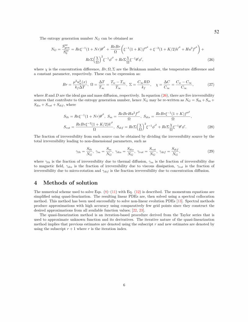
The entropy generation number NG can be obtained as

NG =S′′′genS′′′0

= Reξ−1(1 +Nr)θ′2

+ ReBr

Ω

(ξ−1(1 +K)f ′′

2+ ξ−2(1 +K/2)h′

2+Ha2f ′

2)

+

ReΣ(χ

Ω

)2ξ−1φ′

2+ReΣχ

Ωξ−1θ′φ′, (26)

where χ is the concentration difference, Br,Ω,Σ are the Brinkman number, the temperature difference anda constant parameter, respectively. These can be expression as:

Br = µ2u2w(x)

kf∆T , Ω = ∆TT∞

= Tw − T∞T∞

, Σ = C∞RDkf

, χ = ∆CC∞

= Cw − C∞C∞

, (27)

where R and D are the ideal gas and mass diffusion, respectively. In equation (26), there are five irreversibilitysources that contribute to the entropy generation number, hence NG may be re-written as NG = Sth+Sm+Sdis + Srot + Sdif , where

Sth = Reξ−1(1 +Nr)θ′2, Sm = ReBrHa2f ′

2

Ω , Sdis = ReBrξ−1(1 +K)f ′′2

Ω ,

Srot = ReBrξ−2(1 +K/2)h′2

Ω , Sdif = ReΣ(χ

Ω

)2ξ−1φ′

2+ReΣχ

Ωξ−1θ′φ′. (28)

The fraction of irreversibility from each source can be obtained by dividing the irreversibility source by thetotal irreversibility leading to non-dimensional parameters, such as

γth = SthNG

, γm = SmNG

, γdis = SdisNG

, γrot = SrotNG

, γdif = SdifNG

, (29)

where γth is the fraction of irreversibility due to thermal diffusion, γm is the fraction of irreversibility dueto magnetic field, γdis is the fraction of irreversibility due to viscous dissipation, γrot is the fraction ofirreversibility due to micro-rotation and γdif is the fraction irreversibility due to concentration diffusion.

4 Methods of solutionThe numerical scheme used to solve Eqs. (8)–(11) with Eq. (12) is described. The momentum equations aresimplified using quasi-liearization. The resulting linear PDEs are, then solved using a spectral collocationmethod. This method has been used successfully to solve non-linear evolution PDEs [13]. Spectral methodsproduce approximations with high accuracy using comparatively few grid points since they construct thedesired approximations from all available function values; [22, 23].

The quasi-linearization method is an iteration-based procedure derived from the Taylor series that isused to approximate unknown function and its derivatives. The iterative nature of the quasi-linearizationmethod implies that previous estimates are denoted using the subscript r and new estimates are denoted byusing the subscript r + 1 where r is the iteration index.

6

52

Using the quasi-linearization method on Eqs. (8)–(11) with Eq. (12) result in expanded linear PDEs

a0,rf′′′r+1 + a1,r(η, ξ)f ′′r+1 + a2,r(η, ξ)f ′r+1 + a3,r(η, ξ)fr+1 + a4,rh

′r+1 + a5,r(η, ξ)θr+1 +

a6,r(η, ξ)φr+1 − ξ(1− ξ)∂f ′

∂ξ= R1,r(η, ξ), (30)

b0,rh′′r+1 + b1,r(η, ξ)h′r+1 + b2,r(η, ξ)hr+1 + b3,r(η, ξ)fr+1 + b4,r(η, ξ)f ′r+1 + b5,r(η, ξ)f ′′r+1 −

ξ(1− ξ)∂h∂ξ

= R2,r(η, ξ), (31)

c0,rθ′′r+1 + c1,r(η, ξ)θ′r+1 + c2,r(η, ξ)θr+1 + c3,r(η, ξ)fr+1 + c4,r(η, ξ)f ′r+1 + c5,r(η, ξ)f ′′r+1 +

c6,r(η, ξ)h′r+1 + c7,r(η, ξ)φ′r+1 − ξ(1− ξ)∂θ

∂ξ= R3,r(η, ξ), (32)

d0,rφ′′r+1 + d1,r(η, ξ)φ′r+1 + d2,r(η, ξ)φr+1 + d3,r(η, ξ)fr+1 + d4,r(η, ξ)f ′r+1 + d5,r(η, ξ)θ′′r+1 −

ξ(1− ξ)∂φ∂ξ

= R4,r(η, ξ). (33)

The boundary conditions can be expressed as

fr+1(0, ξ) = s, f ′r+1(0, ξ) = 1, θr+1(0, ξ) = 1, hr+1(0, ξ) = −nf ′′r+1(0, ξ), φr+1(0, ξ) = 1,f ′r+1(∞, ξ)→ 0, hr+1(∞, ξ)→ 0, θr+1(∞, ξ)→ 0, φr+1(∞, ξ)→ 0, (34)

where the coefficients in Eqs. (30)–(33) are

a0,r = (1 +K), a1,r(η, ξ) = η

2 (1− ξ) + ξfr, a2,r(η, ξ) = −2ξf ′r − ξHa2,

a3,r(η, ξ) = ξf ′′r , a4,r(η, ξ) = K, a5,r(η, ξ) = ξwt, a6,r(η, ξ) = ξwc, (35)

b0,r = (1 +K/2), b1,r(η, ξ) = η

2 (1− ξ) + ξfr, b2,r(η, ξ) = 12(1− ξ)− ξf ′r − 2ξK, b3,r(η, ξ) = ξh′r,

b4,r(η, ξ) = −ξhr, b5,r = −ξK, (36)

c0,r = 1 +Nr

Pr, c1,r(η, ξ) = η

2 (1− ξ) + ξfr + ξNbφ′r + 2ξNtθ′r, c2,r(η, ξ) = −ξf ′r + ξQ0,

c3,r(η, ξ) = ξθ′r, c4,r(η, ξ) = −ξθr, c5,r(η, ξ) = 2Ecf ′′r ,

c6,r(η, ξ) = 2Ecξ

(1 +K/2)h′r, c7,r(η, ξ) = ξNbθ′r, (37)

d0,r = 1Sc, d1,r(η, ξ) = η

2 (1− ξ) + ξfr, d2,r(η, ξ) = −ξf ′r − ξR0,

d3,r(η, ξ) = ξφ′r, d4,r(η, ξ) = −ξφr, d5,r(η, ξ) = Nt

Nbξ, (38)

R1,r(η, ξ) = ξfrf′′r − ξf ′

2

r , R2,r(η, ξ) = ξ(frh′r − f ′rhr),

R3,r(η, ξ) = ξ(frθ′r − f ′rθr) + ξNtθ′2

r + ξNbθ′rφ′r + Ecf ′′

2

r + Ec

ξ(1 +K/2)h′

2

r ,

R4,r(η, ξ) = ξ(frφ′r − f ′rφr). (39)

A wide variety of methods that can be used to solve the linear system (30)–(33). In this study, Chebyshevspectral collocation subject to bivariate Lagrange interpolation is used due to the high accuracy associatedwith this method. The discretization is done through the Gauss-Lobatto collocation points are:

τi = cos(iπ

Nη

), ζj = cos

(jπ

Nξ

)

for i = 0, 1, ..., Nη and j = 0, 1, ..., Nξ. (40)

7

53

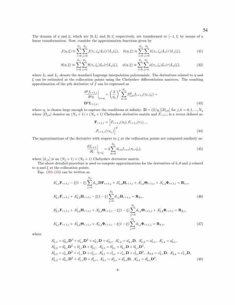
The domain of η and ξ, which are [0, L] and [0, 1] respectively, are transformed to [−1, 1] by means of alinear transformation. Now, consider the approximation functions given by

f(η, ξ) ≈Nη∑

i=0

Nξ∑

j=0f(τi, ζj)Li(τ)Lj(ζ), h(η, ξ) ≈

Nη∑

i=0

Nξ∑

j=0h(τi, ζj)Li(τ)Lj(ζ), (41)

θ(η, ξ) ≈Nη∑

i=0

Nξ∑

j=0θ(τi, ζj)Li(τ)Lj(ζ), φ(η, ξ) ≈

Nη∑

i=0

Nξ∑

j=0φ(τi, ζj)Li(τ)Lj(ζ), (42)

where Li and Lj denote the standard Lagrange interpolation polynomials. The derivatives related to η andξ can be estimated at the collocation points using the Chebyshev differentiation matrices. The resultingapproximation of the pth derivative of f can be expressed as

∂pfr+1,i∂pη

∣∣∣∣η=ηi

=(

2ηe

)p Nη∑

k=0Dpj,kfr+1,i(τk, ζi) =

Dpfr+1,i, (43)

where ηe is chosen large enough to capture the conditions at infinity. D = (2/ηe)[Dj,k] for j, k = 0, 1, ..., Nηwhere [Dj,k] denotes an (Nη + 1)× (Nη + 1) Chebyshev derivative matrix and Fr+1,i is a vector defined as

Fr+1,i =[Fr+1,i(τ0), Fr+1,i(τ1), ...

, Fr+1,i(τNη )]T. (44)

The approximations of the derivative with respect to ζ at the collocation points are computed similarly as:

∂fr+1∂ξ

∣∣∣∣ξ=ξi

= 2Nξ∑

k=0di,kfr+1(τk, ζk), (45)

where [di,k] is an (Nξ + 1)× (Nξ + 1) Chebyshev derivative matrix.The above detailed procedure is used to compute approximations for the derivatives of h, θ and φ related

to η and ξ at the collocation points.Eqs. (30)–(33) can be written as

Ai1,1Fr+1,i − ξ(1− ξ)Nξ∑

j=0di,jDFr+1,j +Ai1,2Hr+1,i +Ai1,3Θr+1,i +Ai1,4Φr+1,i = R1,r,

Ai2,1Fr+1,i +Ai2,2Hr+1,i − ξ(1− ξ)Nξ∑

j=0di,jHr+1,j = R2,r, (46)

Ai3,1Fr+1,i +Ai3,2Hr+1,i +Ai3,3Θr+1,i − ξ(1− ξ)Nξ∑

j=0di,jΘr+1,j +Ai3,4Φr+1,i = R3,r,

Ai4,1Fr+1,i +Ai4,3Θr+1,i +Ai4,4Φr+1,i − ξ(1− ξ)Nξ∑

j=0di,jΦr+1,j = R4,r, (47)

where

Ai1,1 = ai0,rD3 + ai1,rD2 + ai2,rD + ai3,r, Ai1,2 = ai4,rD, Ai1,3 = ai5,r, A

i1,4 = ai6,r,

Ai2,2 = bi0,rD2 + bi1,rD + bi2,r, Ai2,1 = bi3,r + bi4,rD + bi5,rD2,

Ai3,3 = ci0,rD2 + ci1,rD + ci2,r, Ai3,1 = ci3,r + ci4,rD + ci5,rD2, A3,2 = ci6,rD, Ai3,4 = ci7,rD,

Ai4,4 = di0,rD2 + di1,rD + di2,r, Ai4,1 = di3,r + di4,rD, Ai4,3 = di5,rD2, (48)

8

54

with aik,r (k = 0, 1, 2, .., 6) and R1,r = [R1,r(τ0), R1,r(τ1), . . . , R1,r(τNx)]T .

In matrix notation assume that (see Appendix A).The solution is found to be

FF = AA−1RR, (49)

where

B(i,i)1,1 = Ai1,1 − ξ(1− ξ)di,iD, B(i,i)

1,2 = Ai1,2, B(i,i)1,3 = Ai1,3, B

(i,i)1,4 = Ai1,4,

B(i,i)2,1 = Ai2,1, B

(i,i)2,2 = Ai2,2 − ξ(1− ξ)di,iI, B(i,i)

2,3 = Ai2,3, B(i,i)2,4 = Ai2,4,

B(i,i)3,1 = Ai3,1, B

(i,i)3,2 = Ai3,2, B

(i,i)3,3 = Ai3,3 − ξ(1− ξ)di,iI, B(i,i)

3,4 = Ai3,4,

B(i,i)4,1 = Ai4,1, B

(i,i)4,2 = Ai4,2, B

(i,i)4,3 = Ai4,3, B

(i,i)4,4 = Ai4,4 − ξ(1− ξ)di,iI,

B(i,j)1,1 = −ξ(1− ξ)di,jD, B(i,j)

2,2 = −ξ(1− ξ)di,jI,B

(i,j)3,3 = −ξ(1− ξ)di,jI, B(i,j)

4,4 = −ξ(1− ξ)di,jI, i 6= j, (50)

and I represents an (Nη + 1)× (Nη + 1) identity matrix

5 Convergence analysisIn this section, we seek to determine the accuracy of the method through the calculation of the absolutedifference between the successive approximate values of the solutions and their derivatives.

Fig. (2)(a) shows the absolute differences of the successive approximate values for f(η, ξ), h(η, ξ), θ(η, ξ),φ(η, ξ) versus the iterations. It is observed that the solution the absolute difference decreases to ≈ 10−14

after the fifth iterations. Fig. (2)(a) shows the absolute difference of the successive values for the derivativesf ′(η, ξ), h′(η, ξ), θ′(η, ξ), φ′(η, ξ) versus the iterations. It is noted that the absolute difference decreases to≈ 10−13 at sixth iterations

0 5 10 15Iterations

10-15

10-10

10-5

100E

fE

h

E

E

(a)

0 5 10 15Iterations

10-10

10-5

100

Der

ivat

ives

of r

esid

uals

Ef

Eh

E

E

(b)

Figure 2: Convergence graph of (a) f(η, ξ), h(η, ξ), θ(η, ξ) and φ(η, ξ) and (b) f ′(η, ξ), h(η, ξ), θ′(η, ξ) andφ′(η, ξ)

6 Results and discussionThe system described by equations (8)–(11) and (12) is solved by the bivariate spectral quasiliearizationmethod for selected parameter values. The iteration is started from initial approximations which satisfy Eq.

9

55

(12), namely:

f0(η, ξ) = s+ 1− exp(−η), h0(η, ξ) =(

exp(−η))n, (51)

θ0(η, ξ) = exp(−η), φ0(η, ξ) = exp(−η). (52)

We studied the importance of physical parameters for instance the Grashof number (related to temperature)ωt, the heat generation parameter Q0, the material parameter K, the Eckert number Ec and the Grashofnumber (related to concentration) ωc on the velocity f ′(η, ξ), h(η, ξ) microrotation or angular velocity,temperature θ(η, ξ), concentration φ(η, ξ) and the volumetric entropy generation NG(η, ξ) on the micropolarnanofluid. The values of K and ξ are 1 and 0.2 respectively, which are specified in [16]. Unless statedotherwise, values of the rest of parameters for a micropolar laminar fluid flow are Nb = Nt = 0.5, ωt = ωc =1, Nr = 0.2, Ha = 0.5, Sc = 0.94, P r = 6.8, s = 1, Ec = 0.1, Q0 = 0.1, n = 0.5, R0 = 0.3 ([3, 16]).

Table 1 (see Appendix B) represents the computed skin friction f ′′(0, ξ), heat transfer θ′(0, ξ) and themass transfer φ′(0, ξ) for different values of K,Nt,Nb and R0. It is noted that K has a positive relationwith heat transfer and skin friction; however, increased values of K has a negative impact on mass transferand fixing the other parameters. Moreover, we observe that f ′′(0, ξ) increases as Nt increases while θ′(0, xi)and φ′(0, ξ) rates reduce. The skin friction and heat transfer rate vary inversely with Nb whereas Nb haspositive effect on mass transfer rate. The same result holds for f ′′(0, ξ), θ′(0, ξ) and φ′(0, ξ) respect to R0.

Figs. 3(a) and (b) show the behaviour of velocity and angular momentum profiles for various values ofK. We found that the value of material parameter has a positive relation with the velocity profile. It can beclearly noted from Fig. 3(b) that the angular momentum h(ξ, η) decreases when 0 ≤ η ≤ 1. And in regionsfurther from the sheet the angular momentum remains unchanged (η > 1).

The variation of temperature and concentration profiles respect to Eckert number Ec is shown in Figs.4(a) and (b). The temperature is a positive function with the Eckert number. From Fig. 4(b), it is foundthat the the concentration distribution is inversely related to the Eckert number when 0 ≤ η ≤ 1 whereasthe opposite behavior is noted when η > 1.

The changes in the concentration and temperature profiles with varying values of Nr are illustrated inFigs. 5(a) and (b). Fig. 5(a) shows that Nr has a positive relation with temperature profiles, thereforethe boundary layer becomes thickness. In the proximity of the surface, the temperature distribution has anegative slope indicating heat transfer from the surface to the ambient fluid. Fig. 5(b) shows that φ(η, ξ)decrease at a certain values of η.

Figs. 6(a), (b) and (c) depicte the velocity, angular momentum and concentration profiles for differentsolutal buoyancy parameter or local concentration Grashof number ωc. From Fig. 6(a) it is noted thatthevelocity profiles increase as the concentration Grashof number increases. Further, we observe a peak nearthe plate for η = 1.5 and the peak diminishes as ωc is reduced. From Figs. 6(b) and (c), it is noted thatan increment in the solutal Grashof number leads to reduction in the angular momentum and concentrationprofiles; respectively across the boundary layers. Thus, the thickness of the angular and solutal boundarylayer decrease.

The behavioral relationship of the velocity and angular momentum profiles in response to the localGrashof number ωt is shown in Figs. 7 (a) and (b). The figure indicates that the temperature of the thermalboundary layer is enhanced by the local Grashof number which is a phenomenon that can be attributed tothe cooling down of the plate as a result of transferring the temperature by the free convection current tothe free stream from the plate. With regard to the effect of the parameter ωt on the angular momentum,Fig. 7 (b) shows that the angular momentum increases with high values of ωt, peaks at 2 and it falls downuntil vanishes outside the boundary layer. This observation can be traced back to the fact that high valuesof ωt generate strong buoyancy force which, in turns, generate high kinetic energy consumed in negating theflow resistance and as a consequence the angular velocity overshoot.

Fig. 8(a) illustrates the impact of the of the heat generation/absorption parameter Q0 on the temperatureprofile. The figure indicates that an increase in the temperature profile in response to an increase in Q0in the case where the boundary layer generates heat. On the other hand, if the boundary layer absorbsheat, the temperature profiles decreases noticeably with an increase in Q0. Fig. 8(b) depicts the impact of

10

56

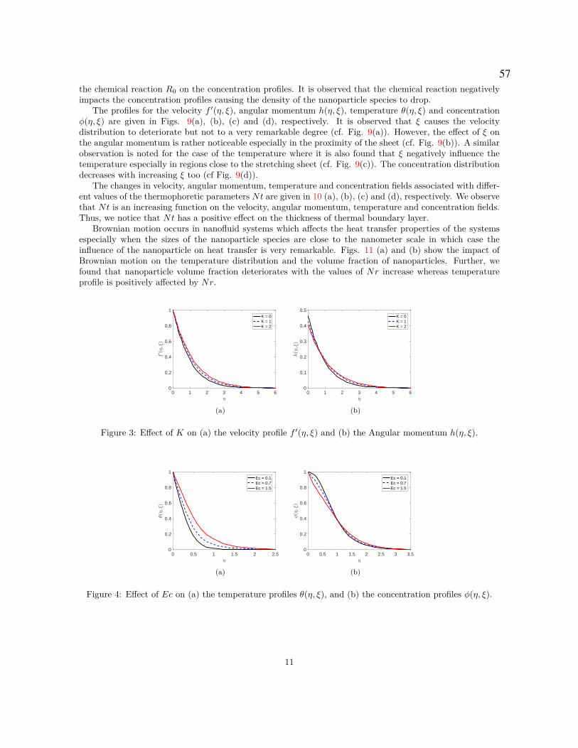
the chemical reaction R0 on the concentration profiles. It is observed that the chemical reaction negativelyimpacts the concentration profiles causing the density of the nanoparticle species to drop.

The profiles for the velocity f ′(η, ξ), angular momentum h(η, ξ), temperature θ(η, ξ) and concentrationφ(η, ξ) are given in Figs. 9(a), (b), (c) and (d), respectively. It is observed that ξ causes the velocitydistribution to deteriorate but not to a very remarkable degree (cf. Fig. 9(a)). However, the effect of ξ onthe angular momentum is rather noticeable especially in the proximity of the sheet (cf. Fig. 9(b)). A similarobservation is noted for the case of the temperature where it is also found that ξ negatively influence thetemperature especially in regions close to the stretching sheet (cf. Fig. 9(c)). The concentration distributiondecreases with increasing ξ too (cf Fig. 9(d)).

The changes in velocity, angular momentum, temperature and concentration fields associated with differ-ent values of the thermophoretic parameters Nt are given in 10 (a), (b), (c) and (d), respectively. We observethat Nt is an increasing function on the velocity, angular momentum, temperature and concentration fields.Thus, we notice that Nt has a positive effect on the thickness of thermal boundary layer.

Brownian motion occurs in nanofluid systems which affects the heat transfer properties of the systemsespecially when the sizes of the nanoparticle species are close to the nanometer scale in which case theinfluence of the nanoparticle on heat transfer is very remarkable. Figs. 11 (a) and (b) show the impact ofBrownian motion on the temperature distribution and the volume fraction of nanoparticles. Further, wefound that nanoparticle volume fraction deteriorates with the values of Nr increase whereas temperatureprofile is positively affected by Nr.

0 1 2 3 4 5 6η

0

0.2

0.4

0.6

0.8

1

f′ (η,ξ)

K = 0K = 1K = 2

(a)

0 1 2 3 4 5 6η

0

0.1

0.2

0.3

0.4

0.5

h(η,ξ)

K = 0K = 1K = 2

(b)

Figure 3: Effect of K on (a) the velocity profile f ′(η, ξ) and (b) the Angular momentum h(η, ξ).

0 0.5 1 1.5 2 2.5η

0

0.2

0.4

0.6

0.8

1

θ(η,ξ)

Ec = 0.1Ec = 0.7Ec = 1.5

(a)

0 0.5 1 1.5 2 2.5 3 3.5η

0

0.2

0.4

0.6

0.8

1

φ(η,ξ)

Ec = 0.1Ec = 0.7Ec = 1.5

(b)

Figure 4: Effect of Ec on (a) the temperature profiles θ(η, ξ), and (b) the concentration profiles φ(η, ξ).

11

57

0 0.5 1 1.5 2η

0

0.2

0.4

0.6

0.8

1

θ(η,ξ)

Nr = 0.1Nr = 0.8Nr = 2

(a)

0 0.5 1 1.5 2 2.5 3 3.5η

0

0.2

0.4

0.6

0.8

1

φ(η,ξ)

Nr = 0.1Nr = 0.8Nr = 2

(b)

Figure 5: Effect of Nr on (a) the temperature profiles θ(η, ξ), and (b) the concentration profiles φ(η, ξ).

0 1 2 3 4 5η

0

0.2

0.4

0.6

0.8

1

f′ (η,ξ)

ωc = 0.1

ωc = 1.5

ωc = 3

(a)

0 1 2 3 4 5η

0

0.1

0.2

0.3

0.4

0.5

0.6

h(η,ξ)

ωc = 0.1

ωc = 1.5

ωc = 3

(b)

0 0.5 1 1.5 2 2.5 3 3.5η

0

0.2

0.4

0.6

0.8

1

φ(η,ξ)

ωc = 0.1

ωc = 1.5

ωc = 3

(c)

Figure 6: Effect of ωc on (a) the velocity profile f ′(η, ξ), (b) the angular momentum h(η, ξ), and (c) theconcentration profiles φ(η, ξ).

0 1 2 3 4 5η

0

0.2

0.4

0.6

0.8

1

f′ (η,ξ)

ωt = 0.5

ωt = 3

ωt = 5

(a)

0 1 2 3 4 5η

0

0.1

0.2

0.3

0.4

h(η,ξ)

ωt = 0.5

ωt = 3

ωt = 5

(b)

Figure 7: Effect of ωt on (a) the velocity profile f ′(η, ξ), and (b) the angular momentum h(η, ξ).

12

58

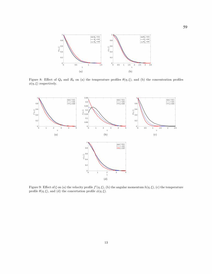
0 0.5 1 1.5η

0

0.2

0.4

0.6

0.8

1

θ(η,ξ)

Q0 = 0.1

Q0 = 0.5

Q0 = 0.9

(a)

0 0.5 1 1.5 2 2.5 3 3.5η

0

0.2

0.4

0.6

0.8

1

φ(η,ξ)

R0 = 0.3

R0 = 0.6

R0 = 0.9

(b)

Figure 8: Effect of Q0 and R0 on (a) the temperature profiles θ(η, ξ), and (b) the concentration profilesφ(η, ξ) respectively.

0 1 2 3 4 5η

0

0.2

0.4

0.6

0.8

1

f′ (η,ξ)

ξ = 0.1ξ = 0.5ξ = 0.9

(a)

0 1 2 3 4 5η

0

0.05

0.1

0.15

0.2

0.25

0.3

0.35

h(η,ξ)

ξ = 0.1ξ = 0.5ξ = 0.9

(b)

0 0.5 1 1.5 2 2.5η

0

0.2

0.4

0.6

0.8

1

θ(η,ξ)

ξ = 0.1ξ = 0.5ξ = 0.9

(c)

0 1 2 3 4η

0

0.2

0.4

0.6

0.8

1

φ(η,ξ)

ξ = 0.1ξ = 0.5ξ = 0.9

(d)

Figure 9: Effect of ξ on (a) the velocity profile f ′(η, ξ), (b) the angular momentum h(η, ξ), (c) the temperatureprofile θ(η, ξ), and (d) the concertation profile φ(η, ξ).

13

59

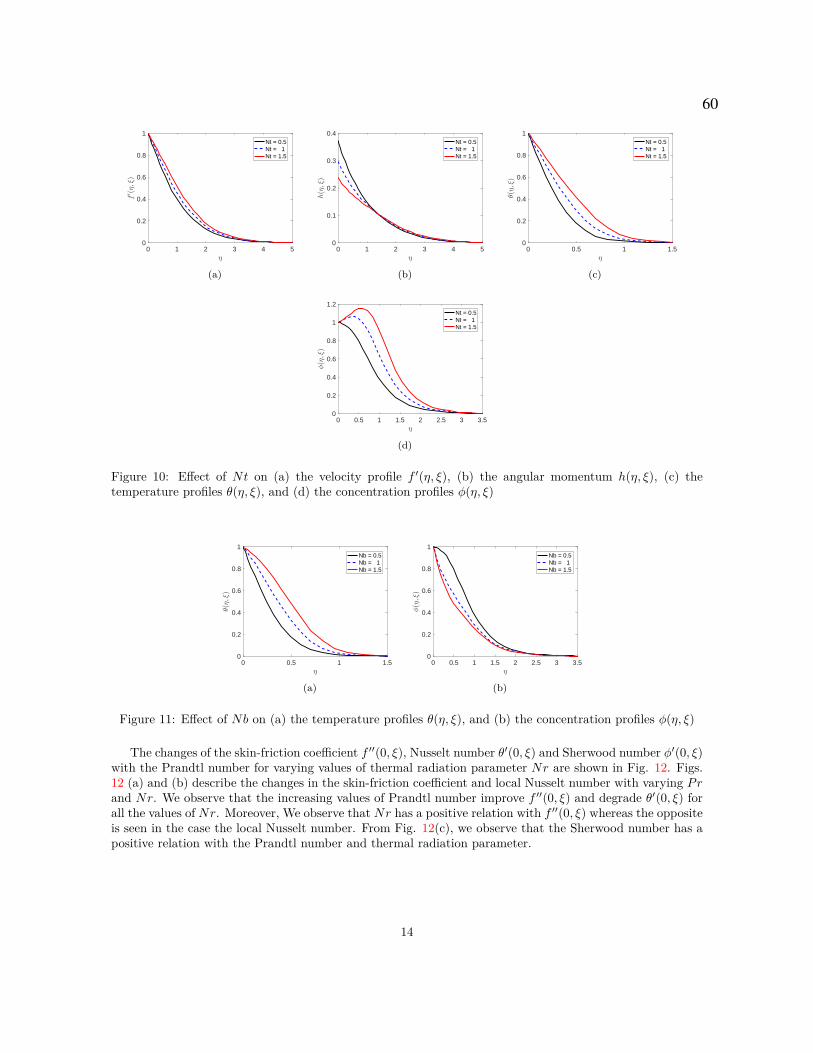
0 1 2 3 4 5η

0

0.2

0.4

0.6

0.8

1f′ (η,ξ)

Nt = 0.5Nt = 1Nt = 1.5

(a)

0 1 2 3 4 5η

0

0.1

0.2

0.3

0.4

h(η,ξ)

Nt = 0.5Nt = 1Nt = 1.5

(b)

0 0.5 1 1.5η

0

0.2

0.4

0.6

0.8

1

θ(η,ξ)

Nt = 0.5Nt = 1Nt = 1.5

(c)

0 0.5 1 1.5 2 2.5 3 3.5η

0

0.2

0.4

0.6

0.8

1

1.2

φ(η,ξ)

Nt = 0.5Nt = 1Nt = 1.5

(d)

Figure 10: Effect of Nt on (a) the velocity profile f ′(η, ξ), (b) the angular momentum h(η, ξ), (c) thetemperature profiles θ(η, ξ), and (d) the concentration profiles φ(η, ξ)

0 0.5 1 1.5η

0

0.2

0.4

0.6

0.8

1

θ(η,ξ)

Nb = 0.5Nb = 1Nb = 1.5

(a)

0 0.5 1 1.5 2 2.5 3 3.5η

0

0.2

0.4

0.6

0.8

1

φ(η,ξ)

Nb = 0.5Nb = 1Nb = 1.5

(b)

Figure 11: Effect of Nb on (a) the temperature profiles θ(η, ξ), and (b) the concentration profiles φ(η, ξ)

The changes of the skin-friction coefficient f ′′(0, ξ), Nusselt number θ′(0, ξ) and Sherwood number φ′(0, ξ)with the Prandtl number for varying values of thermal radiation parameter Nr are shown in Fig. 12. Figs.12 (a) and (b) describe the changes in the skin-friction coefficient and local Nusselt number with varying Prand Nr. We observe that the increasing values of Prandtl number improve f ′′(0, ξ) and degrade θ′(0, ξ) forall the values of Nr. Moreover, We observe that Nr has a positive relation with f ′′(0, ξ) whereas the oppositeis seen in the case the local Nusselt number. From Fig. 12(c), we observe that the Sherwood number has apositive relation with the Prandtl number and thermal radiation parameter.

14

60

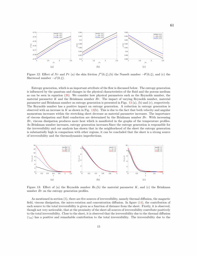
1 1.5 2 2.5Pr

-0.79

-0.78

-0.77

-0.76

-0.75

-0.74

-0.73f′′(0)

Nr = 0.1Nr = 0.2Nr = 0.3

(a)

1 1.5 2 2.5Pr

0.3

0.32

0.34

0.36

0.38

0.4

0.42

0.44

−θ′ (0)

Nr = 0.1Nr = 0.2Nr = 0.3

(b)

1 1.5 2 2.5Pr

0.58

0.59

0.6

0.61

0.62

0.63

0.64

0.65

−φ′ (0)

Nr = 0.1Nr = 0.2Nr = 0.3

(c)

Figure 12: Effect of Nr and Pr (a) the skin friction f ′′(0, ξ),(b) the Nusselt number −θ′(0, ξ), and (c) theSherwood number −φ′(0, ξ).

Entropy generation, which is an important attribute of the flow is discussed below. The entropy generationis influenced by the quantum and changes in the physical characteristics of the fluid and the porous mediumas can be seen in equation (26). We consider how physical parameters such as the Reynolds number, thematerial parameter K and the Brinkman number Br. The impact of varying Reynolds number, materialparameter and Brinkman number on entropy generation is presented in Figs. 13 (a), (b) and (c), respectively.The Reynolds number has a positive impact on entropy generation. A reduction in entropy generation isobserved with an increase in K as shown in Fig. 13(b). This is due to the fact that both velocity and angularmomentum increases within the stretching sheet decrease as material parameter increases. The importanceof viscous dissipation and fluid conduction are determined by the Brinkman number Br. With increasingBr, viscous dissipation produces more heat which is manifested in the graphs of the temperature profiles.As Brinkman number increases, entropy generation increases.Since the entropy generation is responsible forthe irreversibility and our analysis has shown that in the neighborhood of the sheet the entropy generationis substantially high in comparison with other regions, it can be concluded that the sheet is a strong sourceof irreversibility and the thermodynamics imperfections.

0 0.2 0.4 0.6 0.8 1 1.2η

0

2

4

6

8

10

12

14

NG(η,ξ)

Re = 1Re = 3Re = 5

(a)

0 0.2 0.4 0.6 0.8 1η

0

2

4

6

8

NG(η,ξ)

K = 1K = 3K = 6

(b)

0 0.5 1 1.5 2η

0

2

4

6

8

10

NG(η,ξ)

Br = 1Br = 5Br = 9

(c)

Figure 13: Effect of (a) the Reynolds number Re,(b) the material parameter K, and (c) the Brinkmannumber Br on the entropy generation profiles.

As mentioned in section (3), there are five sources of irreversibility, namely thermal diffusion, the magneticfield, viscous dissipation, the micro-rotation and concentration diffusion. In figure (14), the contribution ofeach source to the total irreversibility is given as a function of distance from the sheet. Firstly, it is observed,though not very noticeable, that at the proximity of the sheet all sources of irreversibility contribute positivelyto the total irreversibility. Close to the sheet, it is observed that the irreversibility due to the thermal diffusion(γth) has a positive and remarkable contribution to the total irreversibility. The irreversibility due to the

15

61

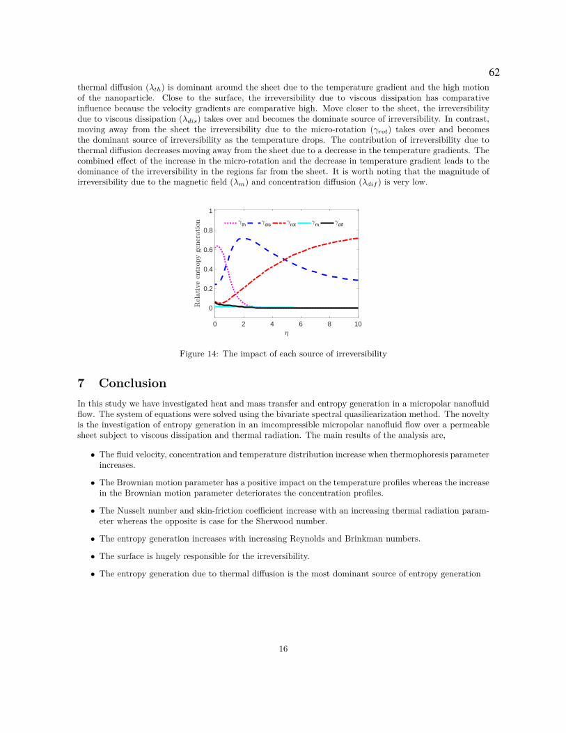
thermal diffusion (λth) is dominant around the sheet due to the temperature gradient and the high motionof the nanoparticle. Close to the surface, the irreversibility due to viscous dissipation has comparativeinfluence because the velocity gradients are comparative high. Move closer to the sheet, the irreversibilitydue to viscous dissipation (λdis) takes over and becomes the dominate source of irreversibility. In contrast,moving away from the sheet the irreversibility due to the micro-rotation (γrot) takes over and becomesthe dominant source of irreversibility as the temperature drops. The contribution of irreversibility due tothermal diffusion decreases moving away from the sheet due to a decrease in the temperature gradients. Thecombined effect of the increase in the micro-rotation and the decrease in temperature gradient leads to thedominance of the irreversibility in the regions far from the sheet. It is worth noting that the magnitude ofirreversibility due to the magnetic field (λm) and concentration diffusion (λdif ) is very low.

0 2 4 6 8 10

0

0.2

0.4

0.6

0.8

1

th dis rot m dif

Figure 14: The impact of each source of irreversibility

7 ConclusionIn this study we have investigated heat and mass transfer and entropy generation in a micropolar nanofluidflow. The system of equations were solved using the bivariate spectral quasiliearization method. The noveltyis the investigation of entropy generation in an imcompressible micropolar nanofluid flow over a permeablesheet subject to viscous dissipation and thermal radiation. The main results of the analysis are,

• The fluid velocity, concentration and temperature distribution increase when thermophoresis parameterincreases.

• The Brownian motion parameter has a positive impact on the temperature profiles whereas the increasein the Brownian motion parameter deteriorates the concentration profiles.

• The Nusselt number and skin-friction coefficient increase with an increasing thermal radiation param-eter whereas the opposite is case for the Sherwood number.

• The entropy generation increases with increasing Reynolds and Brinkman numbers.

• The surface is hugely responsible for the irreversibility.

• The entropy generation due to thermal diffusion is the most dominant source of entropy generation

16

62

Acknowledgement:The authors are grateful to DST-NRF Centre of Excellence-Mathematical and Statistical Sciences, the ClaudeLeon Foundation, DST-NRF Centre of Excellence-Mathematical and Statistical Sciences and the Universityof KwaZulu-Natal for financial support.

References[1] I. Hassanien, R. Gorla, Heat transfer to a micropolar fluid from a non-isothermal stretching sheet with

suction and blowing, Acta Mechanica 84 (1-4) (1990) 191–199.

[2] R. Bhargava, S. Sharma, H. S. Takhar, O. A. Beg, P. Bhargava, Numerical solutions for micropolartransport phenomena over a nonlinear stretching sheet, Nonlinear Anal. Model. Control 12 (2007) 45–63.

[3] K.-L. Hsiao, Micropolar nanofluid flow with mhd and viscous dissipation effects towards a stretchingsheet with multimedia feature, International Journal of Heat and Mass Transfer 112 (2017) 983–990.

[4] K. Das, Effect of chemical reaction and thermal radiation on heat and mass transfer flow of mhdmicropolar fluid in a rotating frame of reference, International journal of heat and mass transfer 54 (15)(2011) 3505–3513.

[5] D. Srinivasacharya, K. H. Bindu, Effect of magnetic field on entropy generation due to micropolar fluidflow in a rectangular duct, Procedia Engineering 127 (2015) 1150–1157.

[6] D. Srinivasacharya, K. H. Bindu, Entropy generation in a micropolar fluid flow through an inclinedchannel, Alexandria Engineering Journal 55 (2) (2016) 973–982.

[7] S. Jangili, N. Gajjela, O. A. Beg, Mathematical modeling of entropy generation in magnetized micropolarflow between co-rotating cylinders with internal heat generation, Alexandria Engineering Journal 55 (3)(2016) 1969–1982.

[8] S. Jangili, S. Adesanya, J. Falade, N. Gajjela, Entropy generation analysis for a radiative micropolarfluid flow through a vertical channel saturated with non-darcian porous medium, International Journalof Applied and Computational Mathematics 3 (4) (2017) 3759–3782.

[9] M. Afridi, M. Qasim, O. Makinde, Second law analysis of boundary layer flow with variable fluidproperties, Journal of Heat Transfer 139 (10) (2017) 104505.

[10] A. Muhammad, O. D. Makinde, Thermodynamics analysis of unsteady mhd mixed convection with slipand thermal radiation over a permeable surface, in: Defect and Diffusion Forum, Vol. 374, Trans TechPubl, 2017, pp. 29–46.

[11] S. O. Adesanya, O. D. Makinde, Irreversibility analysis in a couple stress film flow along an inclinedheated plate with adiabatic free surface, Physica A: Statistical Mechanics and its Applications 432(2015) 222–229.

[12] S. Das, S. Chakraborty, R. Jana, O. Makinde, Entropy analysis of nanofluid flow over a convectivelyheated radially stretching disk embedded in a porous medium, Journal of Nanofluids 5 (1) (2016) 48–58.

[13] S. Motsa, V. Magagula, P. Sibanda, A bivariate chebyshev spectral collocation quasilinearization methodfor nonlinear evolution parabolic equations, The Scientific World Journal 2014.

[14] G. Makanda, S. Shaw, P. Sibanda, Effects of radiation on mhd free convection of a casson fluid froma horizontal circular cylinder with partial slip in non-darcy porous medium with viscous dissipation,Boundary Value Problems 2015 (1) (2015) 75.

17

63

[15] A. Ishak, R. Nazar, I. Pop, Mixed convection stagnation point flow of a micropolar fluid towards astretching sheet, Meccanica 43 (4) (2008) 411–418.

[16] A. Aurangzaib, A. Kasim, S. S. Mohammad NlF, Soret and dufour effects on unsteady mhd flow of amicropolar fluid in the presence of thermophoresis deposition particle, World Applied Sciences Journal21 (5) (2013) 766–73.

[17] N. Sandeep, C. Sulochana, Dual solutions for unsteady mixed convection flow of mhd micropolar fluidover a stretching/shrinking sheet with non-uniform heat source/sink, Engineering Science and Technol-ogy, an International Journal 18 (4) (2015) 738–745.

[18] Y. Kim, Thermal boundary layer flow of a micropolar fluid past a wedge with constant wall temperature,Acta mechanica 138 (1) (1999) 113–121.

[19] A. Bejan, Entropy generation minimization: The new thermodynamics of finite-size devices and finite-time processes, Journal of Applied Physics 79 (3) (1996) 1191–1218.

[20] M. A. Abbas, Y. Bai, M. M. Rashidi, M. M. Bhatti, Analysis of entropy generation in the flow ofperistaltic nanofluids in channels with compliant walls, Entropy 18 (3) (2016) 90.

[21] A. Bejan, Entropy generation minimization, Advanced Engineering Thermodynamics (2016) 531–600.

[22] J. S. Hesthaven, S. Gottlieb, D. Gottlieb, Spectral methods for time-dependent problems, Vol. 21,Cambridge University Press, 2007.

[23] J. P. Boyd, Chebyshev and Fourier spectral methods, Courier Corporation, 2001.

18

64

Appendix A

AA =

B(0,0)1,1 B

(0,0)1,2 B

(0,0)1,3 B

(0,0)1,4 B

(0,1)1,1

. . . B(0,Nξ)1,1

B(0,0)2,1 B

(0,0)2,2 B

(0,0)2,3 B

(0,0)2,4 B

(0,1)2,2

. . . B(0,Nξ)2,2

B(0,0)3,1 B

(0,0)3,2 B

(0,0)3,3 B

(0,0)3,4 B

(0,1)3,3

. . . B(0,Nξ)3,3

B(0,0)4,1 B

(0,0)4,2 B

(0,0)4,3 B

(0,0)4,4 B

(0,1)4,4

. . . B(0,Nξ)4,4

B(1,0)1,1 B

(1,1)1,1 B

(1,1)1,2 B

(1,1)1,3 B

(1,1)1,4

. . . B(1,Nξ)1,1

B(1,0)2,2 B

(1,1)2,1 B

(1,1)2,2 B

(1,1)2,3 B

(1,1)2,4

. . . B(1,Nξ)2,2

B(1,0)3,3 B

(1,1)3,1 B

(1,1)3,2 B

(1,1)3,3 B

(1,1)3,4

. . . B(1,Nξ)3,3

B(1,0)4,4 B

(1,1)4,1 B

(1,1)4,2 B

(1,1)4,3 B

(1,1)4,4

. . . B(1,Nξ)4,4

. . .. . . . . . . . . . . . . . .

. . .. . .

. . . . . . . . . . . . . . .. . .

. . .. . . . . . . . . . . . . . .

. . .. . .

. . . . . . . . . . . . . . .. . .

B(Nξ,0)1,1 B

(Nξ,1)1,1

. . . B(Nξ,Nξ)1,1 B

(Nξ,Nξ)1,2 B

(Nξ,Nξ)1,3 B

(Nξ,Nξ)1,4

B(Nξ,0)2,2 B

(Nξ,1)2,2

. . . B(Nξ,Nξ)2,1 B

(Nξ,Nξ)2,2 B

(Nξ,Nξ)2,3 B

(Nξ,Nξ)2,4

B(Nξ,0)3,3 B

(Nξ,1)3,3

. . . B(Nξ,Nξ)3,1 B

(Nξ,Nξ)3,2 B

(Nξ,Nξ)3,3 B

(Nξ,Nξ)3,4

B(Nξ,0)4,4 B

(Nξ,1)4,4

. . . B(Nξ,Nξ)4,1 B

(Nξ,Nξ)4,2 B

(Nξ,Nξ)4,3 B

(Nξ,Nξ)4,4

,

FF =

F0

H0

Θ0

Φ0

F1

H1

Θ1

Φ1............

FNξHNξ

ΘNξ

ΦNξ

, RR =

R1,0

R2,0

R3,0

R4,0

R1,1

R2,1

R3,1

R4,1............

R1,Nξ

R2,Nξ

R3,Nξ

R4,Nξ

. (53)

19

65

Appendix B

Table 1: Computed f ′′(0, ξ), −θ′(0, ξ) and − φ′(0, ξ) with various values of K,Nt,Nb and R0 when ξ =0.2, ωt = ωc = 1, Nr = 0.2, Ha = 0.5, Sc = 0.94, P r = 6.8, s = 1, Ec = 0.1, Q0 = 0.1, n = 0.5

K Nt Nb R0 Cfx R1/2 Re−1/2Nux Re−1/2Shx

0.2 −0.915452 1.519181 0.853184

1 0.5 0.5 0.3 −0.858733 1.541030 0.850256

2.5 −0.792516 1.562133 0.848537

0.5 −0.858733 1.541030 0.850256

1 1 0.5 0.3 −0.848969 1.286133 0.751045

1.5 −0.839054 1.132108 0.707963

0.2 −0.848848 1.652673 0.528010

1 0.5 0.5 0.3 −0.858733 1.541030 0.850256

1 −0.860131 1.345855 0.979923

0.1 −0.858106 1.542271 0.834545

1 0.5 0.5 0.3 −0.858733 1.541030 0.850256

1 −0.861379 1.531537 0.909714

20

66

Chapter 4

Entropy generation in viscoelastic nanoflu-

ids with homogeneous-heterogeneous reaction,

partial slip and nonlinear thermal radiation

In Chapter 3, we studied the entropy generation in non-Newtonian fluid flow. In this chapter

we take into account the impact homogeneous-heterogeneous chemical reactions and neglect the

partial slip between nanoparticles and the fluid molecules.

We assume the boundary layer flow of a viscoelastic nanofluid over a stretching sheet with non-

linear thermal radiation. We provide some analysis of the impact of the Bejan number on the

viscoelastic nanofluid flow. A nonlinear thermal radiation is assumed. The spectral quasilineariza-

tion method is used to solve the flow equations.

67

Entropy generation in MHD flow of viscoelastic nanofluids withhomogeneous-heterogeneous reaction, partial slip and nonlinear

thermal radiation

M. Almakki,1 H. Mondal,1 ? P.Sibanda,1 N. Haroun1

ABSTRACT

We investigate the combined effects of homogeneous and heterogeneous reactions in the boundary layer flow of aviscoelastic nanofluid over a stretching sheet with nonlinear thermal radiation. The incompressible fluid is electricallyconducting with an applied a transverse magnetic field. The conservation equations are solved using the spectralquasi-linearization method. This analysis is carried out in order to enhance the system performance, with the source ofentropy generation and the impact of Bejan number on viscoelastic nanofluid due to a partial slip in homogeneous andheterogeneous reactions flow using the spectral quasi-linearization method. Various fluid parameters of interest suchas entropy generation, Bejan number, fluid velocity, shear stress heat and mass transfer rates are studied quantitativelyand their behaviors are depicted graphically. A comparison of the entropy generation due to the heat transfer and thefluid friction is made with the help of the Bejan number. Among the findings reported in this study is that the entropygeneration has a significant impact in controlling the rate of heat transfer in the boundary layer region.

KEYWORD:

Nanofluids; Viscoelastic fluid; Homogeneous–Heterogeneous reactions; Nonlinear thermal radiation

INTRODUCTION

In recent years, nanofluids have attracted a considerable amount of interest due to their novel properties thatmake them potentially useful in a number of industrial applications including transportation, power generation, micro-manufacturing, thermal therapy for cancer treatment, chemical and metallurgical sectors, heating, cooling, ventilation,and air-conditioning. The term nanofluid is used to refer to a solid-liquid mixture with a continuous phase, Choi [1].Nanofluids are used in many areas including oil extraction, cancer therapy and safer surgery by cooling. The two-dimensional boundary layer flow in porous media caused by a stretching surface has received considerable attentionbecause such flows arise in many applications such as in paper industry, aerodynamic extrusion of plastic sheets, hotrolling, wire drawing, glass-fiber production and the manufacture of polymer and rubber sheets, Fisher [2]. Makindeet al. [3] investigated nanofluid flow over a linear stretching sheet with thermophoresis and particle Brownian motion.The Brownian motion and thermophoresis lead to an increase in the rate of heat transfer. However, the opposite wasobserved in the case of the rate of mass transfer. The effect of an applied magnetic field on nanofluids has substantialapplications in chemistry, physics and engineering. These include cooling of continuous filaments, in the process ofdrawing, annealing and thinning of copper wire. Drawing such strips through an electrically conducting fluid subjectto a magnetic field can control the rate of cooling and stretching, thereby furthering the desired characteristics of the

1School of Mathematics, Statistics and Computer Science,University of KwaZulu-Natal, Private Bag X01, Scottsvile, Pietermaritzburg-3209,South Africa

2Corresponding author: hiranmoymondal@yahoo.co.in (H. Mondal)

1

68

final product. Such an application of a linearly stretching sheet of incompressible viscous flow of MHD was discussedby Chamka [4].

It is a well-established fact that all bodies emit thermal radiation when their temperature is greater that zero. Thegreater the bodies temperature, the greater the thermal radiation. As a result of thermal radiation, when two bodiescome in contact with each other, the hotter one transmits heat to the less hotter one until the reach the same temperature.The previously stated sentences on thermal radiation is an informed statement of Prevostis Theory of thermal radiationwhich is regarded as the corner of motion theory of thermal radiation; please refer to Putley [5] for elaborate details.Heat transfer and viscous dissipation of MHD nanaofluid flow through a permeable stretching/shrinking sheet wasinvestigated by Sandeep et al. [6]. Raju et al. [7] was scrutinized the influence of the thermal radiation on ferrofluidacross a flat plate within slip velocity and aligned magnetic field. The effects of thermal radiation in presence ofMHD of nanofluid flow throughout two horizontal rotating plates was studied by Mohsen et al. [8]. They pointedout that Nusselt number has remarkable relation with thermal radiation. The common approach prior studies [6,7, 8] to nonlinear temperature is to simplify it using Taylor serious up to a certain order and accept a truncatederror. Consequently, the complexity of the analysis of a thermal radiation model reduces substantially. The linearapproximation of the nonlinear temperature may lead to inconsistency with realistic practical applications in industryand engineering as the thermal radiation, which is a function of temperature, may be far from being linear in reality.Recent studies attempt at overcoming the over simplified approach of prior studies to nonlinear thermal radiation byconsidering it as the fourth power of the temperature and the nonlinearity was not resolved using Taylor series. Thecurrent study employ the same approach to nonlinear thermal radiation as [9, 10].

Many chemically reacting systems involve both homogeneous and heterogeneous reactions, with examples occur-ring in combustion, catalysis and biochemical processes. The interaction between the homogeneous reactions in thebulk of the fluid and heterogeneous reactions occurring on some catalytic surfaces is generally very complex, andis involved in the production and consumption of reactant pieces at different rates both within the fluid and the cat-alytic surfaces. The first study on homogeneous and heterogeneous reactions in boundary layer flow was addressed byChaudhary et al [11]. They presented a simple model of homogeneous-heterogeneous reactions for forced convectionnear leading edge of the plate. Merkin [12] used the same model to considered the problem of a homogeneous reactiondefined by cubic auto-catalysis and the heterogeneous reaction by a first order process in the boundary layer flow ofa viscous fluid past a flat plate. A numerical study of the Homogeneous-heterogeneous reactions in micropolar fluidflow from a permeable stretching or shrinking sheet in a porous medium was conducted by Shaw et al. [13]. The studyshown that the solutions are possible for all positive values of the stretching parameter, while solutions are possibleonly for a limited range of values for shrinking surface. Goyal et al. [14] studied the boundary layer flow and heattransfer of viscoelastic nanofluids past a stretching sheet with partial slip condition. A homogeneous-heterogeneousreactions on boundary layer flow of fluid at a stagnation point over a porous stretching sheet take into account the par-tial slip condition was discussed by Mariam et al. [15]. Bachok et al. [16] examined the homogeneous-heterogeneousreactions boundary layer flow close to the stagnation point past a stretching surface. The analytic solution of thehomogeneous-heterogeneous reactions on Powell-Eyring fluid flow through a stretching sheet was addressed by Hayatet al. [17].

Entropy quantifies the molecular disorder (randomness) of systems. The second low of thermodynamics indicatesthat the entropy generation is positively correlated with the irreversible processes; that is, entropy generation (Egen) isalways positive during irreversible processes. On contrary, the entropy of a system stays unchanged during reversibleprocesses. Since the performance of engineering systems deteriorate by irreversible process, it follows that the en-tropy generation affects the performance of such systems negatively. Therefore, the entropy generation is sometimesregarded as a measure of the magnitude of the irreversiblity of a process. Little attention has been paid to the study ofentropy generation and the impact of the Bejan number (Be) on the viscoelastic nanofluid. This study the mechanismsfor generating entropy are related to heat transfer, magnetic field, fluid friction irreversibility and mass transfer. Mirza-zadeh et al. [18] studied the concept of entropy generation and the impact of the Bejan number (Be) on viscoelasticfluid past rotating cylinders. The application of the second law analysis to viscoelastic MHD flow through a stretchingsheet was scrutinized by Soraya et al. [19]. Adnan et al. [20] analyzed the influence of viscoelasticity on entropygeneration over a stretching plate.

The motivation of the present study is to investigate the entropy generation and Bejan number for steady two-

2

69

dimensional MHD flow, heat and mass transfer of an incompressible viscoelastic nanofluids over a linearly stretchingsheet with homogeneous-heterogeneous chemical reaction and thermal radiation. To the best of the authors knowledgeno paper in the research has so far studied entropy generation and Bejan number in viscoelastic nanofluid over astretching sheet with homogeneous-heterogeneous reaction. The present study has many applications in cooling ofmetallic plate, movement of biological fluids, melt spinning, heat exchangers technology, and oceanography. Precisely,both entropy generation and Bejan number are play a major role in controlling the rate of heat transfer in the proximityof the sheet. The conversations equations are solved using the spectral quasi-linearization method (SQLM). Thebehavior of velocity, temperature, nanoparticles volume fraction, entropy generation and Bejan number are studiedand visualize graphically.

MATHEMATICAL FORMULATION OF THE PROBLEM

Consider an incompressible, steady two-dimensional and hydrodynamics laminar flow of a viscoelastic fluid flowover a linear stretching sheet subject to the magnetic field and homogeneous–heterogeneous chemical reactions. Theflow field is sibject to the effect of external transverse magnetic field of stretching B0. The flow of viscoelasticfluid is restricted to region (y >0) and the stagnation point is fixed at x = 0. The wall and ambient temperatureof the stretching sheet are defined as Tw and T∞ respectively. Ca and Cb are the concentrations homogeneous andheterogeneous reactions for species A and B respectively. In addition the concentration at the ambient is defined as C∞.The velocity near stretching sheet denoted by U(x) = uw(x) = cx, where c represents stretching rate and c >0. Thisstudy considers the interaction between two different types of chemical reaction; such as, a homogeneous (bulk) anda heterogeneous (on sheet) reactions through a boundary layer flow. The reaction between species A and B is given by(see [11, 12] )

A+2B→ 3B, rate = k1CaC2b , (1)

A→ B, rate = ksCa. (2)

Using these assumptions, and the usual boundary layer approximation, the system of equations for the viscoelasticnanofluid are given by:

∂u∂x

+∂v∂y

= 0, (3)

u∂u∂x

+ v∂u∂y

= ν∂ 2u∂y2 −

k0

ρ

[u

∂ 3u∂x∂y2 + v

∂ 3u∂y3 +

∂u∂x

∂ 2u∂y2 −

∂u∂y

∂ 2u∂x∂y

]− σB2

0ρ

u, (4)

u∂T∂x

+ v∂T∂y

= αm∇2T + τ[

DB∂Cb

∂y.∂T∂y

+DT

T∞

(∂T∂y

)2]− 1

ρcp

∂qr

∂y, (5)

u∂Ca

∂x+ v

∂Ca

∂y= DA

∂ 2Ca

∂y2 − k1CaC2b , (6)

u∂Cb

∂x+ v

∂Cb

∂y= DB

∂ 2Cb

∂y2 +DT

T∞

∂ 2T∂y2 + k1CaC2

b , (7)

where αm = k f /(ρcp) f and τ = (ρcp)s/(ρcp) f . Suppose θw = Tw/T∞. Then the temperature can be written as

T = T∞

[1+(θw−1

)θ].

The nonlinear thermal relation qr is relative to heat flux. Applying the Rosseland approximation [9], qr can be writtenas

qr =−4σ∗

3k∗∂T 4

∂y=−16σ∗

3k∗T 3 ∂T

∂y. (8)

3

70

The boundary conditions are:

u =U + k∗1ν∂u∂y, v = 0, T = Tw, DA

∂Ca

∂y= ksCa, DB =

∂Cb

∂y=−ksCa at y = 0,

u = 0, T = T∞, Ca→C∞, Cb→ 0 at y→ ∞. (9)

To simplify the equations we introduce the following similarity transformations:

η =

√cν

y, u = cx f ′(η), v =−√

cν f (η),

θ(η) =T −T∞

Tw−T∞, ξ (η) =

Ca

C∞, φ(η) =

Cb

C∞. (10)

The system of equations (3)–(7) is transformed to:

f ′′′+ f f ′′− f ′2 +α(

f ′′2−2 f ′ f ′′′+ f f ′′′′)−Ha2 f ′ = 0, (11)

[1+Nr

1+(θw−1)θ

3]

θ ′′+3Nr(θw−1)

1+(θw−1)θ2

θ ′2 +Pr f θ ′+

Pr(

Nbθ ′φ ′+Ntθ ′2)= 0, (12)

ξ ′′+Sc f ξ ′−KScξ φ 2 = 0, (13)1

εSc

(φ ′′+

NtNb

θ ′′)+ f φ ′+Kξ φ 2 = 0, (14)

subject to the boundary conditions

f (0) = 0, f ′(0) = 1+λ f ′′(0), θ(0) = 1, ξ ′(0) = Ksξ (0), φ ′(0) =−εKsξ (0),f ′(∞) = 0, θ(∞) = 0, ξ (∞) = 1, φ(∞) = 0, (15)

where a prime refers to differentiation respect to η , λ = k∗1ν√

c/ν , Ks = ks/(DA√

c/ν)

and ε = DA/DB. Thenon-dimensional parameters appearing in Equations (11)–(14) are defined as

α =ck0

ν, Ha2 =

σB20

ρc, Pr =

µcp

k f,

Nr =16σ∗T 3

∞3k∗k f

, Nb =τDBC∞

ν, Nt =

τDT(Tw−T∞

)

νT∞,

K =k1C2

∞c

, Sc =ν

DB, ε =

DA

DB. (16)

Although in many practical scenarios the sizes of the diffusion coefficient of the chemical species of A and B are notequal, they could be of a comparable size. Thus, it is not unrealistic to assume that DA = DB (consequently, ε = 1),[21]. This assumption leads to

ξ (η)+φ(η) = 1. (17)

Consequently, Equations (13) and (14) can be reduced to a single equation as follows

ξ ′′− NtNb

θ ′′+Sc f ξ ′−ScKξ (1−ξ )2 = 0, (18)

with boundary conditions

ξ ′(0) = Ksξ (0), ξ (∞) = 1. (19)

4

71

Hence, the system in Equations (11)–(14) becomes

f ′′′+ f f ′′− f ′2 +α( f ′′2−2 f ′ f ′′′+ f f ′′′′)−Ha2 f ′ = 0, (20)[1+Nr

1+(θw−1)θ

3]

θ ′′+3Nr(θw−1)

1+(θw−1)θ2

θ ′2 +Pr f θ ′+

Pr(

Ntθ ′2−Nbξ ′θ ′)= 0, (21)

ξ ′′− NtNb

θ ′′+Sc f ξ ′−ScKξ (1−ξ )2 = 0, (22)

with the new boundary conditions

f (0) = 0, f ′(0) = 1+λ f ′′(0), f ′(∞) = 0, θ(0) = 1,

θ(∞) = 0, ξ ′(0) = Ksξ (0), ξ (∞) = 1. (23)

The skin friction coefficient C f , the local Nusselt number Nux and the Sherwood number Shx are the most signifi-cant physical quantities which are given by

C f =τw

ρu2w, Nux =

xhw

k(

Tw−T∞

) and Shx =xhm

DBC∞, (24)

where τw, hw and hm are given by

τw = µ(

∂u∂y

)

y=0, hw =−k

(∂T∂y

)

y=0and hm =−DB

(∂Ca

∂y

)

y=0. (25)

Using Equation (9) and Equation (25) the Equation (24) becomes as:

C f Re1/2 = f ′′(0), Re−1/2Nux =−(

1+Nrθ 3w

)θ ′(0) and Re−1/2Shx =−ξ ′(0). (26)

where Re = U(x)xν .

ENTROPY GENERATION ANALYSIS

Entropy measures the chaos of a certain system. Entropy generation depends on procedures reversibility. In isolatedsystems, it is usually the case where there is a rise in entropy over time for reversible reactions. In present days, theapplications of nanofluids in medical and engineering settings, have increased substantially which give more creditsto the studies which investigate the influence of nanoparticles on entropy generation, [22, 23]. In this study the focusis on entropy generation in the viscoelastic nanofluid.

The volumetric rate of local entropy generation, which is based on the second law of thermodynamics, is given by

Egen =k f

T 2∞

((∂T∂y

)2

+16σ∗T 3

3k∗k f

(∂T∂y

)2)+

σB20

T∞u2 +

RDT∞

(∂T∂y

∂Ca

∂y

)+

RDC∞

(∂Ca

∂y

)2

, (27)

where in Equation (27), the first term is irreversibility caused by heat transfer, the second term is the entropygeneration due to the influence of the magnetic field and the third and fourth terms are irreversibility caused bydiffusion effect. The characteristic entropy generation rate is

E0 =k f(∆T)2

x2T 2∞

. (28)

5

72

By using Equation (28) and Equation (10) the entropy generation in dimensionless is given by

NG = Re

1+Nr(

1+χθ)3

θ ′2+

ReBrHa2

χf ′

2+

ReΣχ2 ξ ′

2+

ReΣχ

θ ′ξ ′. (29)

The numbers and parameters in Equation (29) can be obtained as

Re =uw(x)x

ν, Br =

µu2w(x)

k f ∆T,∆T = Tw−T∞,

Σ =C∞RD

k f, χ =

(θw−1

), (30)

Equation (29) can be obtained as a summation of the entropy generation number caused by the heat transfer (N1) andthe entropy generation number caused by both diffusive irreversibility and magnetic field (N2). That is NG = N1 +N2,where

N1 = Re

1+Nr(

1+χθ)3

θ ′2, N2 =

ReBrHa2

χf ′

2+

ReΣχ2 ξ ′

2+

ReΣχ

θ ′ξ ′. (31)

The heat transfer irreversibility, diffusive irreversibility and the magnetic field all contribute to entropy generation.It is therefore worthwhile investigating the conditions under which heat transfer dominates entropy generation. Toinvestigate this question, the Bejan (Be) number is defined as the ratio of entropy generation due to heat transfer andthe entropy generation number.

Be =N1

NG=

11+Φ

, (32)

where Φ = N2N1

represents the irreversibility ratio. Depending on Φ, different factors contribute differently on entropygeneration. When 0 ≤ Φ<1, heat transfer is the most dominant factor in entropy generation. When Φ>1, the irre-versibility diffusive with the magnetic effects dominate on entropy generation. When Φ = 1 heat transfer and diffusionwith magnetic effects contributes equally on entropy generation. The Bejan number takes values in range [0,1] (see[22, 24, 25, 26, 27, 28]). At the extreme when Be = 1 the irreversibility of heat transfer dominates. On the other ex-treme when Be = 0 the combined effects of diffusion and magnetic field dominates the irreversibility. When Be = 0.5,the contribution of heat transfer in entropy generation is the same as the combined contribution of diffusion and mag-netic field in entropy generation. Additionally, the Bejan number Be is considered at the best values of the parametersat which the entropy generation its minimum.

METHODS OF SOLUTION

The quasi-linearization method (QLM) represents the general form of the Newton-Raphson method (Bellman andKalaba [29]). The concept of the QLM is linearization the nonlinear system of equations using the Taylor series byassumption that the difference between the current iteration, r+1, and the previous iteration, r is negligible.

Implementing the quasi-linearization scheme to Equations (20)–(22) subject to the boundary conditions (23), givesthe iterative schemes:

a0,r f ′′′′r+1 +a1,r f ′′′r+1 +a2,r f ′′r+1 +a3,r f ′r+1 +a4,r fr+1 = R f , (33)b0,rθ ′′r+1 +b1,rθ ′r+1 +b2,rθr+1 +b3,r fr+1 +b4,rξ ′r+1 = Rθ , (34)c0,rξ ′′r+1 + c1,rξ ′r+1 + c2,rξr+1 + c3,r fr+1 + c4,rθ ′′r+1 = Rξ , (35)

subject to

6

73

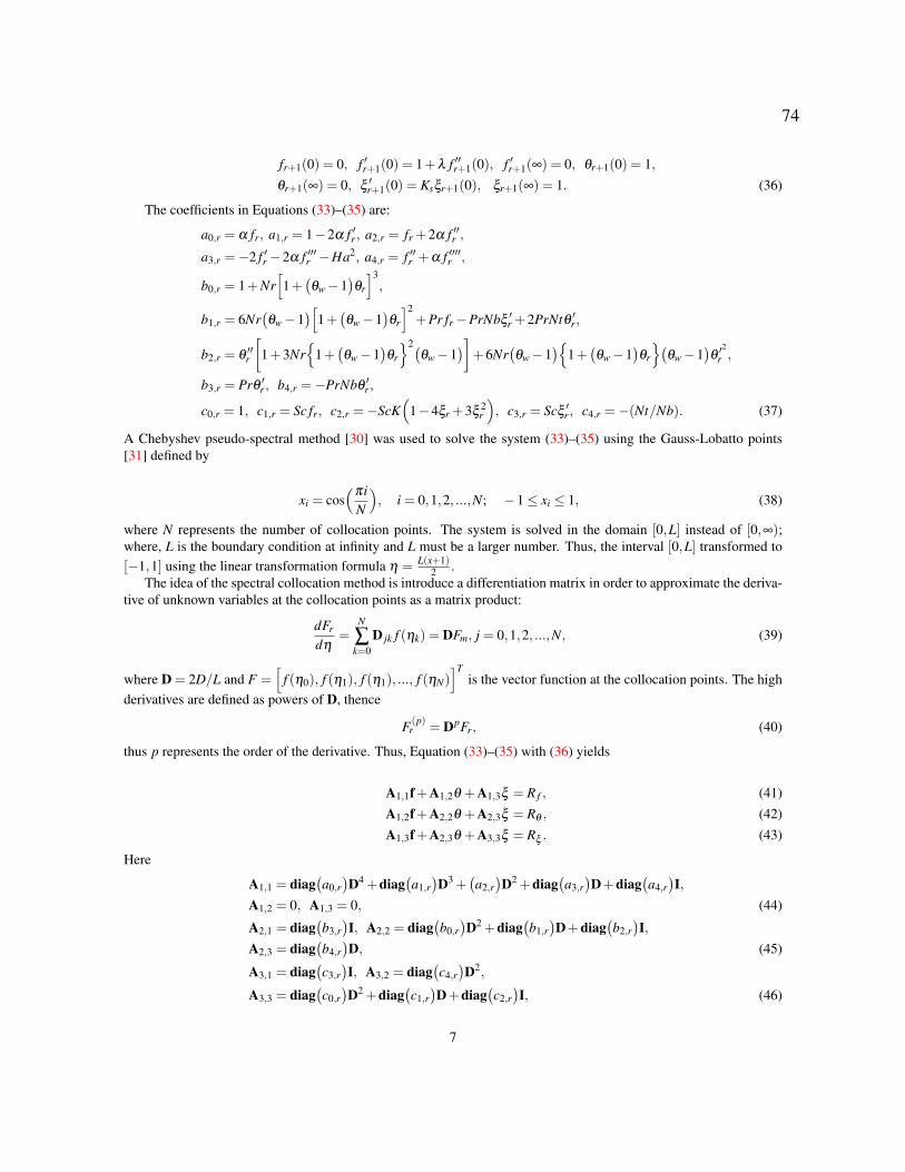
fr+1(0) = 0, f ′r+1(0) = 1+λ f ′′r+1(0), f ′r+1(∞) = 0, θr+1(0) = 1,θr+1(∞) = 0, ξ ′r+1(0) = Ksξr+1(0), ξr+1(∞) = 1. (36)

The coefficients in Equations (33)–(35) are:

a0,r = α fr, a1,r = 1−2α f ′r , a2,r = fr +2α f ′′r ,

a3,r =−2 f ′r−2α f ′′′r −Ha2, a4,r = f ′′r +α f ′′′′r ,

b0,r = 1+Nr[1+(θw−1

)θr

]3,

b1,r = 6Nr(θw−1

)[1+(θw−1

)θr

]2+Pr fr−PrNbξ ′r +2PrNtθ ′r,

b2,r = θ ′′r

[1+3Nr

1+(θw−1

)θr

2(θw−1

)]+6Nr

(θw−1

)1+(θw−1

)θr

(θw−1

)θ ′

2

r ,

b3,r = Prθ ′r, b4,r =−PrNbθ ′r,

c0,r = 1, c1,r = Sc fr, c2,r =−ScK(

1−4ξr +3ξ 2r

), c3,r = Scξ ′r , c4,r =−(Nt/Nb). (37)

A Chebyshev pseudo-spectral method [30] was used to solve the system (33)–(35) using the Gauss-Lobatto points[31] defined by

xi = cos(πi

N

), i = 0,1,2, ...,N; −1≤ xi ≤ 1, (38)

where N represents the number of collocation points. The system is solved in the domain [0,L] instead of [0,∞);where, L is the boundary condition at infinity and L must be a larger number. Thus, the interval [0,L] transformed to[−1,1] using the linear transformation formula η = L(x+1)

2 .The idea of the spectral collocation method is introduce a differentiation matrix in order to approximate the deriva-

tive of unknown variables at the collocation points as a matrix product:

dFr

dη=

N

∑k=0

D jk f (ηk) = DFm, j = 0,1,2, ...,N, (39)

where D = 2D/L and F =[

f (η0), f (η1), f (η1), ..., f (ηN)]T

is the vector function at the collocation points. The highderivatives are defined as powers of D, thence

F(p)r = DpFr, (40)

thus p represents the order of the derivative. Thus, Equation (33)–(35) with (36) yields

A1,1f+A1,2θ +A1,3ξ = R f , (41)A1,2f+A2,2θ +A2,3ξ = Rθ , (42)A1,3f+A2,3θ +A3,3ξ = Rξ . (43)

Here

A1,1 = diag(a0,r)D4 +diag

(a1,r)D3 +

(a2,r)D2 +diag

(a3,r)D+diag

(a4,r)I,

A1,2 = 0, A1,3 = 0, (44)

A2,1 = diag(b3,r)I, A2,2 = diag

(b0,r)D2 +diag

(b1,r)D+diag

(b2,r)I,

A2,3 = diag(b4,r)D, (45)

A3,1 = diag(c3,r)I, A3,2 = diag

(c4,r)D2,

A3,3 = diag(c0,r)D2 +diag

(c1,r)D+diag

(c2,r)I, (46)

7

74

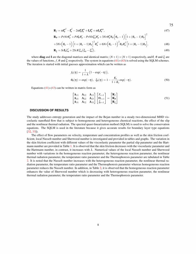
R f = αf′′2

r − f′2

r −2αf′rf′′′r + frf′′r +αfrf′′′′r , (47)

Rθ = PrNtθ ′2

r +Prfrθ ′r−PrNbξ ′rθ ′r +3Nrθ ′′r θ r

(θw−1

)[1+(θw−1)θ r

]2

+3Nr(

θw−1)[

1+(θw−1)θ r

]2θ ′

2

r +6Nr(

θw−1)2

θ rθ ′2

r

[1+(θw−1)θ r

], (48)

Rξ = Scfrξ ′r +2ScKξ r(ξ r−ξ 2

r), (49)

where diag and I are the diagonal matrices and identical matrix; (N+1)× (N+1) respectively, and f, θ and ξ arethe values of functions, f ,θ and ξ respectively. The system in equations (41)–(43) is solved using the SQLM schemes.The iteration is started with initial guesses approximation which can be written as

f0(η) =1

1+λ(1− exp(−η)

),

θ0(η) = exp(−η), ξ0(η) = 1− Ks

1+Ksexp(−η). (50)

Equations (41)–(43) can be written in matrix form as

A11 A12 A13A21 A22 A23A31 A32 A33

Fr+1Θr+1ξr+1

=

R fRθRξ

(51)

DISCUSSION OF RESULTS

The study addresses entropy generation and the impact of the Bejan number in a steady two-dimensional MHD vis-coelastic nanofluid flow that is subject to homogeneous and heterogeneous chemical reactions, the effect of the slipand the nonlinear thermal radiation. The spectral quasi-linearization method (SQLM) is used to solve the conservationequations. The SQLM is used in the literature because it gives accurate results for boundary layer type equations[32, 33]).

The effect of flow parameters on velocity, temperature and concentration profiles as well as the skin friction coef-ficient, local Nusselt number and Sherwood number is investigated and provided in tables and graphs. The variation inthe skin friction coefficient with different values of the viscoelastic parameter the partial slip parameter and the Hart-mann number are provided in Table 1. It is observed that the skin friction decreases with the viscoelastic parameter andthe Hartmann number, in contrast, it increases with λ . Numerical values of the local Nusselt number and Sherwoodnumber with variations in the homogeneous reaction parameter, the heterogeneous reaction parameter, the nonlinearthermal radiation parameter, the temperature ratio parameter and the Thermophoresis parameter are tabulated in Table2. It is noted that the Nusselt number increases with the heterogeneous reaction parameter, the nonlinear thermal ra-diation parameter, the temperature ratio parameter and the Thermophoresis parameter whereas homogeneous reactionparameter reduces the Nusselt number. In addition, in Table 2, it is observed that the homogeneous reaction parameterenhances the value of Sherwood number which is decreasing with heterogeneous reaction parameter, the nonlinearthermal radiation parameter, the temperature ratio parameter and the Thermophoresis parameter.

8

75

Table 1: Numerical values of f ′′(0) with various values of α,λ , and Ha when Nb = 0.5,Sc = 2,Pr = 6,K = 0.5,Ks =1,Nr = 0.5,Nt = 0.2,θw = 1.01

α λ Ha C f Re1/2

0.5 −0.904251160.7 0.3 0.5 −0.974689780.9 −1.06029277

0.1 −1.055904040.2 0.5 0.5 −0.67757017

0.7 −0.58067315

0.2 −0.757611000.2 0.3 0.7 −0.88164753

1 −0.98974875

Table 2: Numerical values of −θ ′(0) and − ξ ′(0) with different values of K,Ks,Nr,θw and Nt when α = 0.2,λ =1,Nb = 0.5, Ha = 0.5,Sc = 2,Pr = 6.

K Ks Nr θw Nt Re−1/2Nux Re−1/2Shx

0.1 −0.44290300 −0.297654510.3 1 0.5 1.01 0.2 −0.45256076 −0.240366550.7 −0.50454819 −0.09720213

0.5 −0.49842157 −0.119276420.5 3 0.5 1.01 0.2 −0.43654921 −0.24314929

7 −0.42046705 −0.28069503

1 −0.39239089 −0.082025080.5 1 1.5 1.01 0.2 −0.36069650 −0.08361434

2 −0.33377872 −0.08566399

1.5 −0.33609133 −0.134364260.5 1 0.5 2 0.2 −0.23905902 −0.14421738

2.5 −0.17085877 −0.14991236

1.5 −0.18792574 −0.151747830.5 1 0.5 1.01 2 −0.14148245 −0.17675215

2.5 −0.11188459 −0.19531184

Figures (1) illustrates the effect of the viscoelastic parameter on the velocity, temperature and concentration profileswhile other parameters are kept fixed. It is observed that an increase in the viscoelastic parameter leads to a decrease inthe velocity and concentration profiles respectively, whereas the temperature profile is positively related to viscoelasticparameter.

The variability on the velocity, temperature and concentration profiles with various values of the partial slip pa-rameter is displayed in Figures (2). It is noted that the influence of increasing partial slip parameter shifts streamline toboundary layer such that the momentum boundary layer becomes thicker. Therefore, partial slip parameter decreasesthe boundary layer velocity and concentration while the temperature increases with partial slip parameter.

Figure (3) shows the effect of different values of the Hartmann number on the velocity, temperature and con-centration profiles. It is observed that an increase in the Hartmann number leads to reduction in both velocity andconcentration profiles whereas it leads to an increase in temperature profile. The depreciation in velocity profile canbe attributed to the presence of Lorentz force which prevails over the boundary layer when Hartmann number increasesand thus leads to an increase in the viscous force which, in turn, resists velocity profile.

The effects of various values of the Brownian motion parameter on the temperature and concentration profiles

9

76

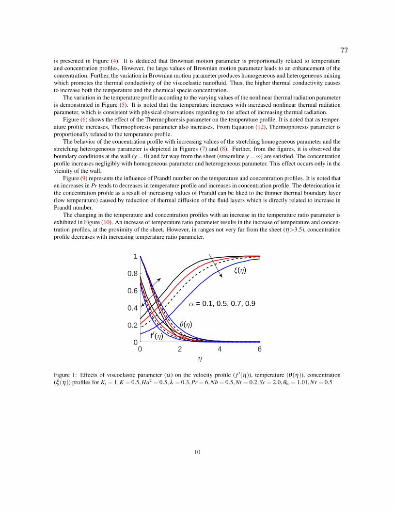
is presented in Figure (4). It is deduced that Brownian motion parameter is proportionally related to temperatureand concentration profiles. However, the large values of Brownian motion parameter leads to an enhancement of theconcentration. Further, the variation in Brownian motion parameter produces homogeneous and heterogeneous mixingwhich promotes the thermal conductivity of the viscoelastic nanofluid. Thus, the higher thermal conductivity causesto increase both the temperature and the chemical specie concentration.

The variation in the temperature profile according to the varying values of the nonlinear thermal radiation parameteris demonstrated in Figure (5). It is noted that the temperature increases with increased nonlinear thermal radiationparameter, which is consistent with physical observations regarding to the affect of increasing thermal radiation.

Figure (6) shows the effect of the Thermophoresis parameter on the temperature profile. It is noted that as temper-ature profile increases, Thermophoresis parameter also increases. From Equation (12), Thermophoresis parameter isproportionally related to the temperature profile.

The behavior of the concentration profile with increasing values of the stretching homogeneous parameter and thestretching heterogeneous parameter is depicted in Figures (7) and (8). Further, from the figures, it is observed theboundary conditions at the wall (y = 0) and far way from the sheet (streamline y = ∞) are satisfied. The concentrationprofile increases negligibly with homogeneous parameter and heterogeneous parameter. This effect occurs only in thevicinity of the wall.

Figure (9) represents the influence of Prandtl number on the temperature and concentration profiles. It is noted thatan increases in Pr tends to decreases in temperature profile and increases in concentration profile. The deterioration inthe concentration profile as a result of increasing values of Prandtl can be liked to the thinner thermal boundary layer(low temperature) caused by reduction of thermal diffusion of the fluid layers which is directly related to increase inPrandtl number.

The changing in the temperature and concentration profiles with an increase in the temperature ratio parameter isexhibited in Figure (10). An increase of temperature ratio parameter results in the increase of temperature and concen-tration profiles, at the proximity of the sheet. However, in ranges not very far from the sheet (η>3.5), concentrationprofile decreases with increasing temperature ratio parameter.

0 2 4 6η

0

0.2

0.4

0.6

0.8

1

θ(η)

f′(η)

ξ(η)

α = 0.1, 0.5, 0.7, 0.9

Figure 1: Effects of viscoelastic parameter (α) on the velocity profile ( f ′(η)), temperature (θ(η)), concentration(ξ (η)) profiles for Ks = 1,K = 0.5,Ha2 = 0.5,λ = 0.3,Pr = 6,Nb = 0.5,Nt = 0.2,Sc = 2.0,θw = 1.01,Nr = 0.5

10

77

0 2 4 6η

0

0.2

0.4

0.6

0.8

1

θ(η)

ξ(η)

λ = 0.1,0.3,0.5,0.7

f′(η)

Figure 2: Effects of the partial slip parameter (λ ) on the velocity ( f ′(η)), temperature (θ(η)) and concentration(ξ (η)) profiles for Ks = 1,K = 0.5,Ha2 = 0.5,α = 0.2,Pr = 6,Nb = 0.5,Nt = 0.2,Sc = 2.0,θw = 1.01,Nr = 0.5

0 2 4 6η

0

0.2

0.4

0.6

0.8

1

θ(η)

ξ(η)

Ha = 0.2, 0.5, 0.7, 1

f′(η)

Figure 3: Effects of the Hartmann number (Ha) on the velocity ( f ′(η)), temperature (θ(η)) and concentration (ξ (η))profiles for Ks = 1,K = 0.5,λ = 0.3,α = 0.2,Pr = 6,Nb = 0.5,Nt = 0.2,Sc = 2.0,θw = 1.01,Nr = 0.5

11

78

0 2 4 6η

0

0.2

0.4

0.6

0.8

1ξ(η)

Nb = 0.5,1, 1.5, 2

θ(η)

Figure 4: Effects of the Brownian mention parameter (Nb) on the velocity ( f ′(η)), temperature (θ(η)) and concentra-tion (ξ (η)) profiles for Ks = 1,K = 0.5,λ = 0.3,α = 0.2,Pr = 6,Ha2 = 0.5,Nt = 0.2,Sc = 2.0,θw = 1.01,Nr = 0.5

0 2 4 6 8η

0

0.2

0.4

0.6

0.8

1

θ(η) Nr = 0.5, 1, 1.5, 2

Figure 5: Effects of the thermal radiation parameter (Nr) on the temperature profile (θ(η)) for Ks = 1,K = 0.5,λ =0.3,α = 0.2,Pr = 6,Ha2 = 0.5,Nt = 0.2,Sc = 2.0,θw = 1.01,Nb = 0.5

12

79

0 2 4 6 8η

0

0.2

0.4

0.6

0.8

1

θ(η)

Nt = 0.5, 1.5, 2, 2.5

Figure 6: Effects of the Thermophoresis parameter (Nt) on the temperature profile (θ(η)) for Ks = 1,K = 0.5,λ =0.3,α = 0.2,Pr = 6,Ha2 = 0.5,Nr = 0.5,Sc = 2.0,θw = 1.01,Nb = 0.5

0 2 4 6 8η

0

0.2

0.4

0.6

0.8

1

ξ(η)

K= 0.1, 0.3, 0.5, 0.7

Figure 7: Effects of the stretching homogeneous parameter (K) on the concentration profile (ξ (η)) for Ks = 1,Nt =0.2,λ = 0.3,α = 0.2,Pr = 6,Ha2 = 0.5,Nr = 0.5,Sc = 2.0,θw = 1.01,Nb = 0.5

13

80

0 2 4 6 8η

0

0.2

0.4

0.6

0.8

1

ξ(η)

Ks = 0.5, 1, 3, 7

Figure 8: Effects of the stretching heterogeneous parameter (Ks) on the concentration profile (ξ (η)) for K = 0.5,Nt =0.2,λ = 0.3,α = 0.2,Pr = 6,Ha2 = 0.5,Nr = 0.5,Sc = 2.0,θw = 1.01,Nb = 0.5

0 2 4 6 8η

0.2

0.4

0.6

0.8

1

4.9 5

0.970.98

ξ(η)

Pr = 3, 5, 7,9

θ(η)

Figure 9: Effects of the Prandtl number (Pr) on the temperature (θ(η)) concentration (ξ (η)) profiles for K = 0.5,Nt =0.2,λ = 3.5,α = 0.2,Ks = 1,Ha2 = 0.5,Nr = 0.5,Sc = 2.0,θw = 1.01,Nb = 0.5

14

81

0 5 10η

0

0.2

0.4

0.6

0.8

1ξ(η)

θw

= 1.01, 1.5, 2, 2.5

θ(η)

Figure 10: Effects of the temperature ratio parameter (θw) on the temperature (θ(η)) concentration (ξ (η)) profilesfor K = 0.5,Nt = 0.2,λ = 3.5,α = 0.2,Ks = 1,Ha2 = 0.5,Nr = 0.5,Sc = 2.0,Pr = 6,Nb = 0.5

The behavior of dimensionless entropy generation profile represents one of the most important characteristic of thisstudy. The variation in entropy generation profile is examined and exhibited in different figures with different valuesof the pertinent parameters, namely, the Hartmann number, the Brinkman number, the dimensionless parameter, theviscoelastic parameter, the Reynolds number and the partial slip parameter respectively. It is worth noting that Figures(11)–(17) provide several ways to control the entropy generation number.

Figure (11) shows the effect of the Hartmann number on the entropy generation number. An increase in Hartmannnumber results in the increment of the entropy generation number. In the neighborhood of the sheet vicinity, Hartmannnumber has significant impact on the entropy generation number, whereas at regions far away from the sheet, theHartmann number has slight effect on the entropy generation number. This effect tends to increase the resistance ofthe fluid motion, consequently the heat transfer rates increase, which result in an increase in the entropy generationnumber. However, at far from the sheet vicinity, the influence of Hartmann number is insignificant.

Figure (12) displays entropy generation with the Brinkman number, which represents a measure of the significanceof the heat produced by viscous heating proportional to heat transported by molecular conduction. An increase in theBrinkman number tends to increase the entropy generation number especially in the vicinity of the sheet. Heat gen-erated bey viscous dissipation prevails through the heat transported via the molecular conduction in the neighborhoodof the sheet. In the vicinity of the sheet, essential heat generation occurs over the boundary layer of the moving fluidparticles, which trends the entropy generation number to enhance by increasing the degree of disorder of the system.

The variation in the entropy generation number with different values of the Prandtl number is illustrated in Figure(13). It is noted that an increase in the Prandtl number leads to an increases in the entropy generation number in theneighborhood to the sheet. However, in ranges not very far from the sheet, entropy generation number decreases withincreasing the value of the Prandtl number. Furthermore, in the proximity of the sheet, the entropy generation numberincreases with a rise in the Prandtl number because the concentration profile shows a substantial decrease as Prandtlnumber increases (see Figure 9). Further, for a fixed value of Prandtl number, entropy generation number decreasesgradually as moving away from the sheet until it extinguishes completely.

Figure (14) shows the behavior of the entropy generation number with the temperature ratio parameter. It can beobserved that in the neighborhood of the sheet, the entropy generation number decreases with increasing the temper-ature ratio parameter. However, in ranges not very far from the sheet, an increases in the temperature ratio parametertends to an increase in the entropy generation number. Moreover, in the proximity of the sheet, the entropy generationnumber decreases with a rise in the temperature ratio parameter because the concentration profile illustrates a greatincrease with increasing the temperature ratio parameter (see Figure 10). Further, for a fixed value of the temperatureratio parameter, the entropy generation number increases gradually as moving away from the sheet.

15

82

Figure (15) shows the influence of the viscoelastic parameter on the entropy generation number. It is worth notingthat the entropy generation number is proportionally related to the viscoelastic parameter especially in the vicinity ofthe sheet. Figure (16) relates the entropy generation number with the Reynolds number. It is noted that the Reynoldsnumber has remarkable effects on the entropy generation number as an increase in the Reynolds number leads to asignificant increase in the entropy generation number, in the vicinity of the sheet. As Reynolds number increases,the entropy generation number caused by the heat transfer dominates the entropy generation number caused by thediffusion effect and the magnetic field in the neighborhood of the stretching sheet. This effect makes the fluid motionmore random to the extent that troubled fluid motions arise. Consequently, the entropy generation number increasesdue to the contribution of heat transfer. Moreover, when Reynolds number increases, the inertia forces are promoted,hence, the values of the viscous forces are decreased. By increasing the value of the Reynolds number, the accelerationof the fluid increases in the vicinity of the sheet. However, far away from the sheet these effects are negligible.

The variation in the entropy generation number with various values of the partial slip parameter is illustrated inFigure (17). It is noted that the entropy generation number decreases when partial slip parameter increase, in thevicinity of the sheet. However, when the distance becomes larger, this effect is negligible.

The entropy generation number can be due to (the diffusion effect and magnetic field) and heat transfer. Therefore,it is legitimate to investigate which of these three factors dominates the entropy generation number. To identity whetherthe entropy generation due to heat transfer dominates over the entropy generation due to (diffusive irreversibility andmagnetic field) (and vice versa), the Bejan number is studied for different physical parameters. Moreover, the Bejannumber can be used to identity the dominant irreversibility: either the heat irreversibilit or the diffusion and themagnetic field irreversibility.

0 0.5 1 1.5 2 2.5 3η

0

1

2

3

4

NG(η)

Ha = 0.1, 0.2, 0.3, 0.5

Figure 11: Effects of the Hartmann number (Ha2) on the entropy generation number (NG(η)) with Ks = 1,K = 0.5,λ =0.2,α = 0.2,Nb = 0.5,Nt = 0.2,Nr = 0.5,Pr = 6,Sc = 2.0,θw = 1.01,Re = 1,Br = 8,χ = 0.2,Σ = 0.01.

16

83

0 1 2 3 4η

0

0.5

1

1.5

NG(η)

Br = 2, 4, 6, 8

Figure 12: Effects of the Brinkman number (Br) on the entropy generation number (NG(η)) with Ks = 1,K = 0.5,λ =2,α = 0.2,Nb = 0.5,Nt = 0.2,Nr = 0.5,Pr = 6,Sc = 4.0,θw = 1.01,Re = 1,Ha2 = 0.5,χ = 0.2,Σ = 0.01.

0 1 2 3 4η

0

1

2

3

4

NG(η)

Pr = 3, 5, 7, 9

Figure 13: Effects of the Prandtl number (Pr) on the entropy generation number (NG(η)) with Ks = 1,K = 0.5,λ =0.2,α = 0.2,Nb = 0.5,Nt = 0.2,Nr = 0.5,Pr = 6,Sc = 4.0,θw = 1.9,Br = 4,Re = 1,Ha2 = 0.5,χ = 0.2,Σ = 0.01.

17

84

0 2 4 6 8η

0

0.2

0.4

0.6

0.8

1

NG(η)

θw

= 1.5, 2, 2.5, 2.7

Figure 14: Effects of the temperature ratio parameter (θw) on the entropy generation number (NG(η)) with Ks = 1,K =0.5,λ = 2,α = 0.2,Nb = 0.5,Nt = 0.2,Nr = 0.5,Pr = 6,Sc = 2.0,χ = 0.2,Re = 1,Ha2 = 0.5,Br = 4,Σ = 0.01.

0 1 2 3 4 5 6η

0

0.5

1

1.5

NG(η)

α = 1, 1.5, 2, 2.5

Figure 15: Effects of the viscoelastic parameter (α) on the entropy generation number (NG(η)) with Ks = 1,K =0.5,λ = 2,Nb = 0.5,Nt = 0.2,Nr = 0.5,Pr = 6,Sc = 2.0,θw = 1.01,Re = 1,Ha2 = 0.5,Br = 8,χ = 0.2,Σ = 0.01.

18

85

0 1 2 3 4 5η

0

1

2

3

4

NG(η)

Re = 0.5, 1.2, 2, 2.5

Figure 16: Effects of the Reynolds number (Re) on the entropy generation number (NG(η)) with Ks = 1,K = 0.5,λ =2,Nb = 0.5,Nt = 0.2,Nr = 0.5,Pr = 6,Sc = 2.0,θw = 1.01,α = 0.2,Ha2 = 0.5,Br = 8,χ = 0.2,Σ = 0.01.

0 1 2 3 4η

0

2

4

6

8

NG(η)

λ = 0.1, 0.3, 0.5, 07

Figure 17: Effects of the partial slip parameter (λ ) on the entropy generation number (NG(η)) with Ks = 1,K =0.5,Re = 1,Nb = 0.5,Nt = 0.2,Nr = 0.5,Pr = 6,Sc = 2.0,θw = 1.01,α = 0.2,Ha2 = 0.5,Br = 8,χ = 0.2,Σ = 0.01.

19

86

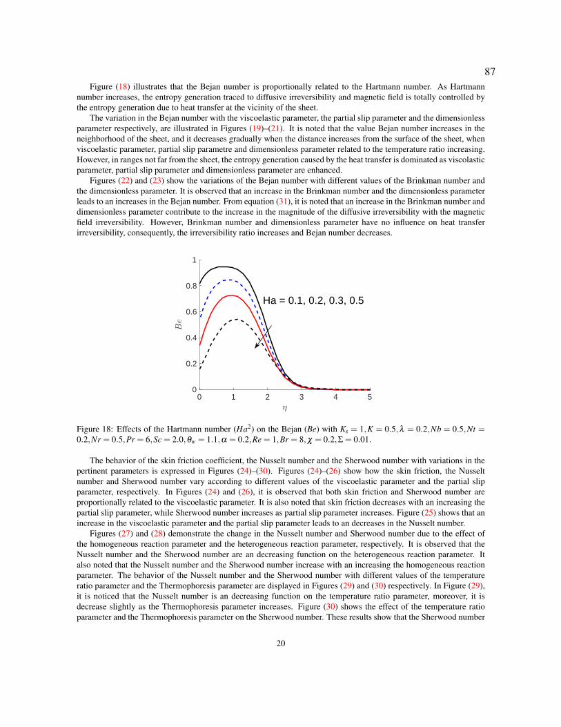
Figure (18) illustrates that the Bejan number is proportionally related to the Hartmann number. As Hartmannnumber increases, the entropy generation traced to diffusive irreversibility and magnetic field is totally controlled bythe entropy generation due to heat transfer at the vicinity of the sheet.

The variation in the Bejan number with the viscoelastic parameter, the partial slip parameter and the dimensionlessparameter respectively, are illustrated in Figures (19)–(21). It is noted that the value Bejan number increases in theneighborhood of the sheet, and it decreases gradually when the distance increases from the surface of the sheet, whenviscoelastic parameter, partial slip parametre and dimensionless parameter related to the temperature ratio increasing.However, in ranges not far from the sheet, the entropy generation caused by the heat transfer is dominated as viscolasticparameter, partial slip parameter and dimensionless parameter are enhanced.

Figures (22) and (23) show the variations of the Bejan number with different values of the Brinkman number andthe dimensionless parameter. It is observed that an increase in the Brinkman number and the dimensionless parameterleads to an increases in the Bejan number. From equation (31), it is noted that an increase in the Brinkman number anddimensionless parameter contribute to the increase in the magnitude of the diffusive irreversibility with the magneticfield irreversibility. However, Brinkman number and dimensionless parameter have no influence on heat transferirreversibility, consequently, the irreversibility ratio increases and Bejan number decreases.

0 1 2 3 4 5η

0

0.2

0.4

0.6

0.8

1

Be

Ha = 0.1, 0.2, 0.3, 0.5

Figure 18: Effects of the Hartmann number (Ha2) on the Bejan (Be) with Ks = 1,K = 0.5,λ = 0.2,Nb = 0.5,Nt =0.2,Nr = 0.5,Pr = 6,Sc = 2.0,θw = 1.1,α = 0.2,Re = 1,Br = 8,χ = 0.2,Σ = 0.01.

The behavior of the skin friction coefficient, the Nusselt number and the Sherwood number with variations in thepertinent parameters is expressed in Figures (24)–(30). Figures (24)–(26) show how the skin friction, the Nusseltnumber and Sherwood number vary according to different values of the viscoelastic parameter and the partial slipparameter, respectively. In Figures (24) and (26), it is observed that both skin friction and Sherwood number areproportionally related to the viscoelastic parameter. It is also noted that skin friction decreases with an increasing thepartial slip parameter, while Sherwood number increases as partial slip parameter increases. Figure (25) shows that anincrease in the viscoelastic parameter and the partial slip parameter leads to an decreases in the Nusselt number.

Figures (27) and (28) demonstrate the change in the Nusselt number and Sherwood number due to the effect ofthe homogeneous reaction parameter and the heterogeneous reaction parameter, respectively. It is observed that theNusselt number and the Sherwood number are an decreasing function on the heterogeneous reaction parameter. Italso noted that the Nusselt number and the Sherwood number increase with an increasing the homogeneous reactionparameter. The behavior of the Nusselt number and the Sherwood number with different values of the temperatureratio parameter and the Thermophoresis parameter are displayed in Figures (29) and (30) respectively. In Figure (29),it is noticed that the Nusselt number is an decreasing function on the temperature ratio parameter, moreover, it isdecrease slightly as the Thermophoresis parameter increases. Figure (30) shows the effect of the temperature ratioparameter and the Thermophoresis parameter on the Sherwood number. These results show that the Sherwood number

20

87

0 1 2 3 4 5 6η

0

0.2

0.4

0.6

0.8

Be

α = 0.1, 0.5, 0.7, 0.9

Figure 19: Effects of the viscoelastic parameter (α) on the Bejan (Be) with Ks = 1,K = 0.5,λ = 2,Nb = 0.5,Nt =0.2,Nr = 0.5,Pr = 6,Sc = 2.0,θw = 1.01,Ha2 = 0.5,Re = 1,Br = 8,χ = 0.1,Σ = 0.1.

0 1 2 3 4 5 6η

0

0.1

0.2

0.3

0.4

0.5

Be

λ = 0.1, 0.3, 0.5, 0.7

Figure 20: Effects of the partial slip parameter (λ ) on the Bejan (Be) with Ks = 1,K = 0.5,α = 0.2,Nb = 0.5,Nt =0.2,Nr = 0.5,Pr = 6,Sc = 2.0,θw = 1.01,Ha2 = 0.5,Re = 1,Br = 8,χ = 0.1,Σ = 0.1.

21

88

0 1 2 3 4 5 6η

0

0.2

0.4

0.6

0.8

1

Be

χ = 0.1, 0.2, 0.3, 0.4

Figure 21: Effects of the dimensionless parameter (ξ ) on the Bejan (Be) with Ks = 1,K = 0.5,α = 0.2,λ = 2,Nb =0.5,Nt = 0.2,Nr = 0.5,Pr = 6,Sc = 2.0,θw = 1.01,Ha2 = 0.5,Re = 1,Br = 1,Σ = 0.1.

0 1 2 3 4 5η

0

0.1

0.2

0.3

0.4

0.5

Be

Br = 2, 4, 6, 8

Figure 22: Effects of the Brinkman number (Br) on the Bejan (Be) with Ks = 1,K = 0.5,α = 0.2,λ = 2,Nb= 0.5,Nt =0.2,Nr = 0.5,Pr = 6,Sc = 2.0,θw = 1.01,Ha2 = 0.5,Re = 1,χ = 0.1,Σ = 0.1.

22

89

0 1 2 3 4 5 6η

0

0.2

0.4

0.6

0.8

Be

Σ = 0.01, 0.02, 0.03, 0.04

Figure 23: Effects of the dimensionless parameter (Σ) on the Bejan (Be) with Ks = 1,K = 0.5,α = 0.2,λ = 2,Nb =0.5,Nt = 0.2,Nr = 0.5,Pr = 6,Sc = 2.0,θw = 1.01,Ha2 = 0.5,Re = 1,χ = 0.1,Br = 8.

decreases with an increasing temperature ration parameter, whereas it is increase as the Thermophoresis parameterincreases.

0.1 0.2 0.3 0.4 0.5λ

0.6

0.7

0.8

0.9

1

1.1

1.2

−f′′(0)

α = 0.1, 0.2, 0.3, 0.4

Figure 24: Effect of the viscoelastic parameter (α) and the partial slip parameter (λ ) on the skin friction f ′′(0) withKs = 1,K = 0.5,Nb = 0.5,Nt = 0.2,Nr = 0.5,Pr = 6,Sc = 2.0,θw = 1.01,Ha2 = 0.5.

23

90

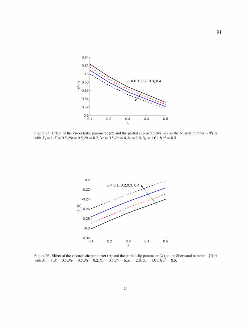
0.1 0.2 0.3 0.4 0.5λ

0.5

0.52

0.54

0.56

0.58

0.6

0.62

0.64

−θ′ (0)

α = 0.1, 0.2, 0.3, 0.4

Figure 25: Effect of the viscoelastic parameter (α) and the partial slip parameter (λ ) on the Nusselt number −θ ′(0)with Ks = 1,K = 0.5,Nb = 0.5,Nt = 0.2,Nr = 0.5,Pr = 6,Sc = 2.0,θw = 1.01,Ha2 = 0.5.

0.1 0.2 0.3 0.4 0.5λ

-0.32

-0.3

-0.28

-0.26

-0.24

-0.22

-0.2

−ξ′ (0)

α = 0.1, 0.2,0.3, 0.4

Figure 26: Effect of the viscoelastic parameter (α) and the partial slip parameter (λ ) on the Sherwood number −ξ ′(0)with Ks = 1,K = 0.5,Nb = 0.5,Nt = 0.2,Nr = 0.5,Pr = 6,Sc = 2.0,θw = 1.01,Ha2 = 0.5.

24

91

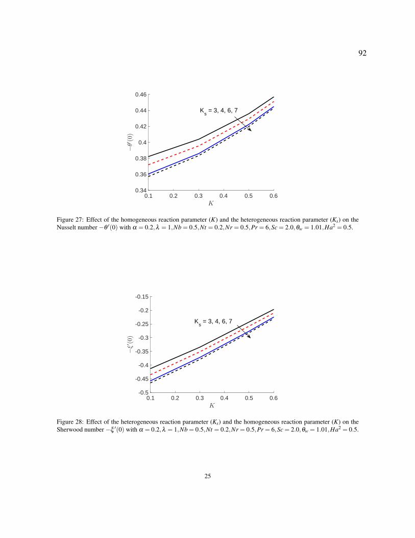
0.1 0.2 0.3 0.4 0.5 0.6K

0.34

0.36

0.38

0.4

0.42

0.44

0.46

−θ′ (0)

Ks = 3, 4, 6, 7

Figure 27: Effect of the homogeneous reaction parameter (K) and the heterogeneous reaction parameter (Ks) on theNusselt number −θ ′(0) with α = 0.2,λ = 1,Nb = 0.5,Nt = 0.2,Nr = 0.5,Pr = 6,Sc = 2.0,θw = 1.01,Ha2 = 0.5.

0.1 0.2 0.3 0.4 0.5 0.6K

-0.5

-0.45

-0.4

-0.35

-0.3

-0.25

-0.2

-0.15

−ξ′ (0)

Ks = 3, 4, 6, 7

Figure 28: Effect of the heterogeneous reaction parameter (Ks) and the homogeneous reaction parameter (K) on theSherwood number −ξ ′(0) with α = 0.2,λ = 1,Nb = 0.5,Nt = 0.2,Nr = 0.5,Pr = 6,Sc = 2.0,θw = 1.01,Ha2 = 0.5.

25

92

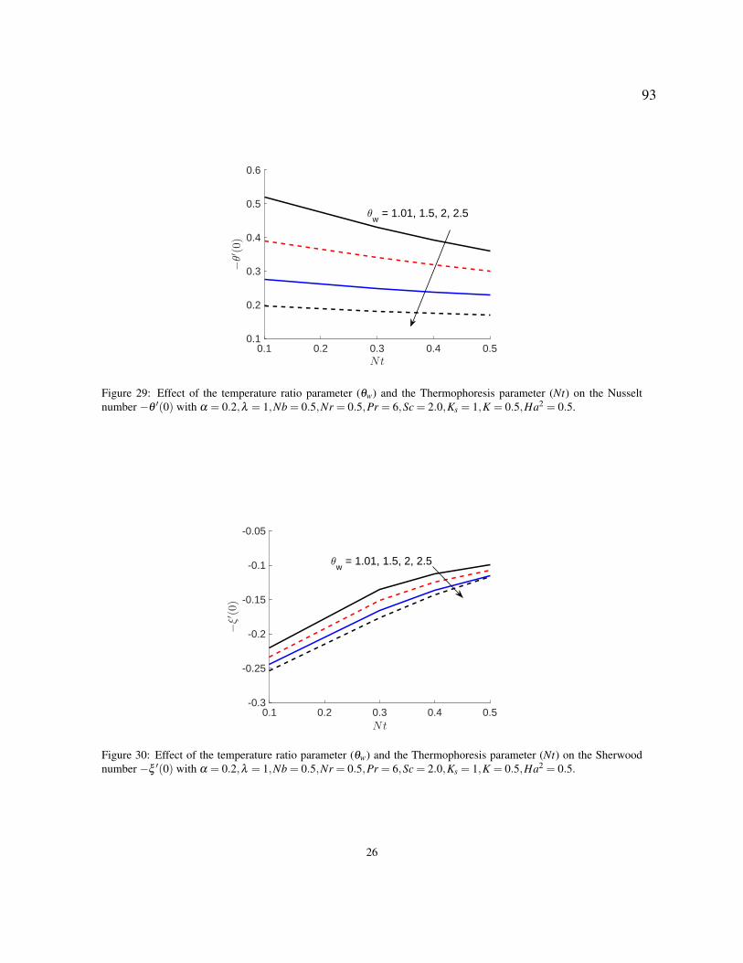
0.1 0.2 0.3 0.4 0.5Nt

0.1

0.2

0.3

0.4

0.5

0.6

−θ′ (0)

θw

= 1.01, 1.5, 2, 2.5

Figure 29: Effect of the temperature ratio parameter (θw) and the Thermophoresis parameter (Nt) on the Nusseltnumber −θ ′(0) with α = 0.2,λ = 1,Nb = 0.5,Nr = 0.5,Pr = 6,Sc = 2.0,Ks = 1,K = 0.5,Ha2 = 0.5.

0.1 0.2 0.3 0.4 0.5Nt

-0.3

-0.25

-0.2

-0.15

-0.1

-0.05

−ξ′ (0)

θw

= 1.01, 1.5, 2, 2.5

Figure 30: Effect of the temperature ratio parameter (θw) and the Thermophoresis parameter (Nt) on the Sherwoodnumber −ξ ′(0) with α = 0.2,λ = 1,Nb = 0.5,Nr = 0.5,Pr = 6,Sc = 2.0,Ks = 1,K = 0.5,Ha2 = 0.5.

26

93

CONCLUSIONS

A numerical model was developed to study the entropy generation in MHD flow of viscoelastic nanofluids withhomogeneous-heterogeneous reaction, partial slip and nonlinear thermal radiation. The resulting partial differentialequations have been solved using the spectral quasi-linearization method. The graphical results were obtained to illus-trate the details of flow, heat and mass transfer characteristics and their dependence on some physical parameter. Thefollowing conclusions can be derived from the numerical results:

(i) Enhancement occur in thermal boundary layer, whereas the concentration and momentum boundary layer re-duces when the viscoelastic parameter increases.(ii) The velocity and concentration profiles are strongly influenced by the magnetic field in the momentum boundarylayer, which decreases with the increase in the Hartmann number and reverse trends are seen for temperature profile.(iii) The velocity and concentration profiles are reduced due to increase the partial slip parameter but reverse effectsare seen for temperature profiles.(iv) The impact of the Brownian motion parameter and thermophoresis parameter on temperature are similar, whilethe effects on nanoparticles volume fraction are opposite for increasing the Brownian motion parameter.(v) The effect of nonlinear thermal radiation is to increase temperature in the thermal boundary layer.(vi) The concentration at the surface decreased with the strengths of the homogeneous and heterogeneous reactions.(vii) The Prandtl number and temperature ratio parameter show a quite opposite behavior for temperature and concen-tration profile.(viii) The entropy generation number decreases with the increase of viscoelastic parameter and partial slip parameter,while the entropy generation number increases with the increase of Brinkman number and Reynolds number.(ix) The Bejan number is strongly affected by variations in the viscoelastic parameter and dimensionless Brinkmangroups.(x) The local Nusselt number and Sherwood number decrease with the increase in homogeneous and heterogeneouschemical reaction parameter.

ACKNOWLEDGEMENT

The authors are grateful to the Claude Leon Foundation, DST-NRF Centre of Excellence-Mathematical and StatisticalSciences and the University of KwaZulu-Natal for financial support.

NOMENCLATURE

A homogeneous chemical reactionB heterogeneous chemical reactionBr Brinkman numberB0 magnetic field strength (kg s−2A−1)C concentration (kgm−3)Ca concentration of homogeneous chemical

reaction A (kgm−3)Cb concentration of heterogeneous chemical

reaction B (kgm−3)Cw concentration at surface (kgm−3)C∞ ambient concentration (kgm−3)c,k∗1 are constantscp specific heat (m2s−2K−1)DA diffusion coefficient of specie A (kgm−1s−1)DB diffusion coefficient of specie B (kgm−1s−1)

DT Thermophoretic diffusion coefficient(kgm−1s−1K−1)

Egen volumetric entropy generation per unit length(Wm−4K−1)

E0 dimensionless entropy generation ratef dimensionless velocityHa Hartmann numberhm mass flux (kgm−2s−1)hw heat flux (Wm−2)K the stretch of the homogeneous reactionKs the stretch of the heterogeneous reactionk f thermal conductivity (Wm−1K−1)ks,k1 constants ratek0 material fluid parameterk∗ mean absorption coefficient

27

94

Nb Brownian mention parameterNr thermal radiation parameterNt Thermophoresis parameterp pressure (kgm−1s−2)Pr Prandtl numberqr radiative heat flux (kgm−2)Re Reynolds numberSc Schmidt number

T temperature (K)Tw uniform surface temperature (K)T∞ ambient temperature (K)∆T difference between (TW −T∞)(K)U(x) velocity of the stretching sheet (ms−1)u,v velocity components (ms−1)x,y rectangular coordinate axis (m)

GREEK SYMBOLS

α viscoelastic parameterαm thermal diffusion of fluid (m2s−1)ε the ration diffusion coefficientη dimensionless variableθ dimensionless temperatureθw similarity variable related to the energy equationλ dimensionless velocity slip parameterµ dynamic viscosity (kgm−1s−1)ν kinematic viscosity (m2s−1)ξ dimensionless concentration of specie Aρ density of fluid (kgm−3)

(ρcp) f heat capacity of base fluid(ρcp)s heat capacity of the nanoparticleΣ dimensionless parameterσ electrical conductivity (Ω−1m−1)σ∗ Steaffan-Boltzman constantτ ratio of nanoparticle heat capacityτw shear stress at the surfaceφ dimensionless concentration of specie Bχ constant parameter

References

[1] Choi, S. U., Eastman, J. A. Enhancing thermal conductivity of fluids with nanoparticles. Technical report,Argonne National Lab., IL (United States) (1995)

[2] Valyi, E. I. Extrusion of plastics. US Patent 5,082,604 (1992)

[3] Makinde, O. D., Aziz, A. Boundary layer flow of a nanofluid past a stretching sheet with a convective boundarycondition. International Journal of Thermal Sciences 50, 7, 1326–1332 (2011)

[4] Chamkha, A. J. Mhd flow of a uniformly stretched vertical permeable surface in the presence of heat gen-eration/absorption and a chemical reaction. International Communications in Heat and Mass Transfer 30, 3,413–422 (2003)

[5] Putley, E. The development of thermal imaging systems. Recent Advances in Medical Thermology, 151–166.Springer (1984)

[6] Sandeep, N., Sulochana, C., Kumar, B. R. Mhd boundary layer flow and heat transfer past a stretching/shrinkingsheet in a nanofluid. Journal of Nanofluids 4, 4, 512–517 (2015)

[7] Sandeep, N., Raju, C., Sulochana, C., Sugunamma, V. Effects of aligned magneticfield and radiation on theflow of ferrofluids over a flat plate with non-uniform heat source/sink. International Journal of Science andEngineering 8, 2, 151–158 (2015)

[8] Sheikholeslami, M., Ganji, D. D., Javed, M. Y., Ellahi, R. Effect of thermal radiation on magnetohydrodynamicsnanofluid flow and heat transfer by means of two phase model. Journal of Magnetism and Magnetic Materials374, 36–43 (2015)

[9] Hayat, T., Muhammad, T., Alsaedi, A., Alhuthali, M. Magnetohydrodynamic three-dimensional flow of vis-coelastic nanofluid in the presence of nonlinear thermal radiation. Journal of Magnetism and Magnetic Materials385, 222–229 (2015)

28

95

[10] Animasaun, I., Raju, C., Sandeep, N. Unequal diffusivities case of homogeneous–heterogeneous reactions withinviscoelastic fluid flow in the presence of induced magnetic-field and nonlinear thermal radiation. AlexandriaEngineering Journal 55, 2, 1595–1606 (2016)

[11] Chaudhary, M., Merkin, J. Homogeneous-heterogeneous reactions in boundary-layer flow: Effects of loss ofreactant. Mathematical and computer modelling 24, 3, 21–28 (1996)

[12] Merkin, J. A model for isothermal homogeneous-heterogeneous reactions in boundary-layer flow. Mathematicaland Computer Modelling 24, 8, 125–136 (1996)

[13] Shaw, S., Kameswaran, P. K., Sibanda, P. Homogeneous-heterogeneous reactions in micropolar fluid flow froma permeable stretching or shrinking sheet in a porous medium. Boundary Value Problems 2013, 1, 77 (2013)

[14] Goyal, M., Bhargava, R. Boundary layer flow and heat transfer of viscoelastic nanofluids past a stretching sheetwith partial slip conditions. Applied Nanoscience 4, 6, 761–767 (2014)

[15] Sheikh, M., Abbas, Z. Homogeneous–heterogeneous reactions in stagnation point flow of casson fluid due to astretching/shrinking sheet with uniform suction and slip effects. Ain Shams Engineering Journal (2015)

[16] Bachok, N., Ishak, A., Pop, I. On the stagnation-point flow towards a stretching sheet with homogeneous–heterogeneous reactions effects. Communications in Nonlinear Science and Numerical Simulation 16, 11, 4296–4302 (2011)

[17] Hayat, T., Imtiaz, M., Alsaedi, A. Effects of homogeneous-heterogeneous reactions in flow of powell-eyringfluid. Journal of Central South University 22, 8, 3211–3216 (2015)

[18] Mirzazadeh, M., Shafaei, A., Rashidi, F. Entropy analysis for non-linear viscoelastic fluid in concentric rotatingcylinders. International Journal of Thermal Sciences 47, 12, 1701–1711 (2008)

[19] Aıboud, S., Saouli, S. Entropy analysis for viscoelastic magnetohydrodynamic flow over a stretching surface.International Journal of Non-Linear Mechanics 45, 5, 482–489 (2010)

[20] Butt, A. S., Munawar, S., Ali, A., Mehmood, A. Effect of viscoelasticity on entropy generation in a porousmedium over a stretching plate. World Applied Sciences Journal 17, 4, 516–523 (2012)

[21] Chaudhary, M., Merkin, J. A simple isothermal model for homogeneous-heterogeneous reactions in boundary-layer flow. i equal diffusivities. Fluid dynamics research 16, 6, 311–333 (1995)

[22] Awad, M. M. A review of entropy generation in microchannels. Advances in Mechanical Engineering 7, 12,1687814015590297 (2015)

[23] Bejan, A. Advanced engineering thermodynamics. John Wiley & Sons (2016)

[24] Awad, M. M. A new definition of bejan number. Thermal Science 16, 4, 1251–1253 (2012)

[25] Awad, M. M., Lage, J. L. Extending the bejan number to a general form. Thermal Science 17, 2, 631–633 (2013)

[26] Awad, M. M. Hagen number versus bejan number. Thermal Science 17, 4, 1245–1250 (2013)

[27] Awad, M. M. An alternative form of the darcy equation. Thermal Science 18, suppl. 2, 617–619 (2014)

[28] Awad, M. M. The science and the history of the two bejan numbers. International Journal of Heat and MassTransfer 94, 101–103 (2016)

[29] Bellman, R. E., Kalaba, R. E. Quasilinearization and nonlinear boundary-value problems (1965)

[30] Agbaje, T., Mondal, S., Makukula, Z., Motsa, S., Sibanda, P. A new numerical approach to mhd stagnation pointflow and heat transfer towards a stretching sheet. Ain Shams Engineering Journal (2016)

29

96

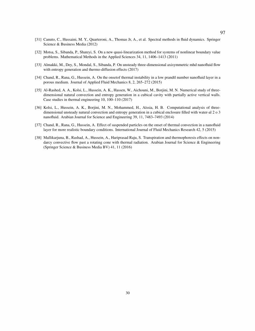
[31] Canuto, C., Hussaini, M. Y., Quarteroni, A., Thomas Jr, A., et al. Spectral methods in fluid dynamics. SpringerScience & Business Media (2012)

[32] Motsa, S., Sibanda, P., Shateyi, S. On a new quasi-linearization method for systems of nonlinear boundary valueproblems. Mathematical Methods in the Applied Sciences 34, 11, 1406–1413 (2011)

[33] Almakki, M., Dey, S., Mondal, S., Sibanda, P. On unsteady three-dimensional axisymmetric mhd nanofluid flowwith entropy generation and thermo-diffusion effects (2017)

[34] Chand, R., Rana, G., Hussein, A. On the onsetof thermal instability in a low prandtl number nanofluid layer in aporous medium. Journal of Applied Fluid Mechanics 8, 2, 265–272 (2015)

[35] Al-Rashed, A. A., Kolsi, L., Hussein, A. K., Hassen, W., Aichouni, M., Borjini, M. N. Numerical study of three-dimensional natural convection and entropy generation in a cubical cavity with partially active vertical walls.Case studies in thermal engineering 10, 100–110 (2017)

[36] Kolsi, L., Hussein, A. K., Borjini, M. N., Mohammed, H., Aıssia, H. B. Computational analysis of three-dimensional unsteady natural convection and entropy generation in a cubical enclosure filled with water-al 2 o 3nanofluid. Arabian Journal for Science and Engineering 39, 11, 7483–7493 (2014)

[37] Chand, R., Rana, G., Hussein, A. Effect of suspended particles on the onset of thermal convection in a nanofluidlayer for more realistic boundary conditions. International Journal of Fluid Mechanics Research 42, 5 (2015)

[38] Mallikarjuna, B., Rashad, A., Hussein, A., Hariprasad Raju, S. Transpiration and thermophoresis effects on non-darcy convective flow past a rotating cone with thermal radiation. Arabian Journal for Science & Engineering(Springer Science & Business Media BV) 41, 11 (2016)

30

97

Chapter 5

Entropy generation in Casson nanofluid flow

with a binary chemical reaction and nonlin-

ear thermal radiation

In Chapter 4, it was assumed that the velocity of the stretching surface is linear. In this chapter

we consider nonlinear velocity to bring the model a step closer to reality. In addition, we also

investigate a binary chemical reaction which is not considered in all previous chapters.

In this chapter we propose a model that captures the behaviour of a steady incompressible MHD

Casson nanofluid flow over a stretching or shrinking sheet. It is assumed that the surface stretches

in the vertical direction with exponential velocity. Subsequently, the model is used to analyse the

entropy generation, heat and mass transfer in the laminar flow near the stagnation point. Viscous

dissipation, nonlinear thermal radiation and a binary chemical reaction are assumed. The spectral

quasiliearization method is used to solve the flow equations.

98

Entropy generation in Casson nanofluid flow with binary

chemical reaction and nonlinear thermal radiation

Mohammed Almakki1, Peri K. Kameswaran 2, Hiranmoy Mondal 1, Precious Sibanda 1

1School of Mathematical Sciences, University of KwaZulu-Natal, Private Bag X01,

Scottsville 3209, Pietermaritzburg, South Africa2 Department of Mathematics, School of Advanced Sciences, VIT University,

Vellore 632014, India

November 29, 2018

1 Abstract

We present a model to describe the flow of an MHD Casson nanofluid over a stretching/shrinkingsurface. The model used to investigate entropy generation and heat transfer in the laminarboundary-layer stagnation point. The flow is subject to an external magnetic field, nonlinearthermal radiation, viscous disipation and binary chemical reaction. The sysyem is solved numer-ically using the spectral local lineralization method. The method is found to be accurate andconvergent. The results show that entropy generation increases with an increase in the Reynoldsnumber and Casson parameter.

Keywords: binary chemical reaction; Casson Nanofluids; Entropy generation; non-linear ther-mal radiation; spectral quasi-linearization method.

2 Introduction

A Casson nanofluid is a fluid that is generated by a suspending solid particles with dimensionsless than 100 nm in a fluid. It has a liquid phase and and a solid phase. It also has enhancedthermophysical properties such as high thermal diffusivity, viscosity, and thermal conductivitycompared to base liquids such as water, oil and ethylene glycol mixture, etc. These fluids havediverse uses in industry, for instance, in fuel cell, biomedicine, nuclear reactors and transporta-tion. The flow of a viscous incompressible fluid driven by a moving surface is encountered in anumber of industrial processes such as in metal and plastic extrusion, glass blowing and polymerextrusion. The study of fluid flow with a binary chemical reaction is encountered in a number oflarge scale manufacturing processes. The flow of fluid with a chemically reacting species over astretching sheet play an important role in metallurgy and chemical engineering industries, suchas food processing and polymer production [1]. All these applications involve some aspects offlow over a stretching sheet, free convection, heat transfer and so on. Running flow reactions

1

99

have a number of advantages over batch processes. The advantages include achieving mixing insmaller time scales, heat transfer is intensified, because the area to volume ration is large. Oxleyet al [2] studied flow on a spinning disk used in the manufacturing of pharmaceuticals. Theyshowed that the spinning disk reactor (SDR) displayed distinct advantages over batch processingin the commercial manufacture of pharmaceuticals. It was further postulated that the SDR iscapable of generating a far higher mixing intensity than a stirred vessel and is also capable ofmaintaining a uniform concentration profiles within a rapidly reacting fluid.

The quality of most industrial products depends on the rate of heat and mass transfer duringcooling. Heat is generated or absorbed during a chemical reaction [3]. Some of the strategies thathave been used for controlling the heat transfer rate include the use of a transverse magnetic field[4] and the use of nanofluids. Nanofluids consist of nanopartices, normally aluminum, gold, ironoxide, platinum, silica, silver etc of sizes ranging from 1 to 100 nanometers suspended in a basefluid to increase/improve the thermal performance of base liquids. Nanofluids have a wide rangeof applications such as in cooling systems, solar water heating and improving diesel generatorefficiency [5].

Another important factor in fluid flow with a chemical reaction is the activation energy. Thisis the minimum energy which must be available for potential reactants to produce a chemicalreaction [6]. We include the activation energy in this model, which most researchers have notincorporated in previous studies. Pal and Mondal [7] investigated the effects of a chemicalreaction on boundary layer flow past a vertical stretching surface with internal heat generation.They found that for positive buoyancy, the local skin friction and mass transfer coefficientsincrease with Eckert and Schmidt numbers while the heat transfer coefficient decreases withboth the Eckert and Schmidt numbers. However, the study did not consider the activationenergy, nanoparticle effects and order of the chemical reaction. These are new aspects thatare incorporated in the current model. Olanrewaju et al [8] studied the effects of internal heatgeneration on a thermal boundary layer with a convective surface boundary condition. Theyobserved that for weak plate heating, the surface temperature increased rapidly as the localinternal heat generation increased. Their model however did not include mass transfer. Reddyet al [9, 10] studied free convection, heat and mass transfer flow in a chemically reactive andradiation absorption fluid in an aligned magnetic filed. The concentration was shown to decreasewith increasing chemical reaction rates which also reduced the solutal boundary layer thickness.It was further noted that increasing the radiation parameter caused a decrease in the fluidvelocity. The velocity attained a peak in the absence of the radiation parameter. Palani et al[11] studied the MHD flow of an upper-convected Maxwell fluid with a higher order chemicalreaction. The main conclusion from this study was that the thickness of the species distributionincreased with increasing order of a chemical reaction. However the study did not incorporateenergy transport including the aspect of activation energy.

In this work, we are interested in investigating entropy generation in MHD Casson nanofluid flowin porous media with binary chemical reaction. In thermodynamical systems, factors such asheat transfer, mass transfer, viscous dissipation and magnetic field may give rise to entropy gen-eration. In many engineering applications, e.g. heat exchangs, electronic cooling, fuel cells andturbomachinery the comprehensive analysis of the flow and thermodynamics is imperative. Thestudy of entropy generation is relevant also in physiological processes. In phoysiological stud-ies, blood pressure is measured periodically when the subjects are conducting physical/mentaltasks. Depending on the temperature of the surrouding environment and the temperature ofthe subjects, heat transfer occurs between the subjects and the environment through sweating,radiation and conduction. Monitoring entropy generation is crucia characterizing such systems

2

100

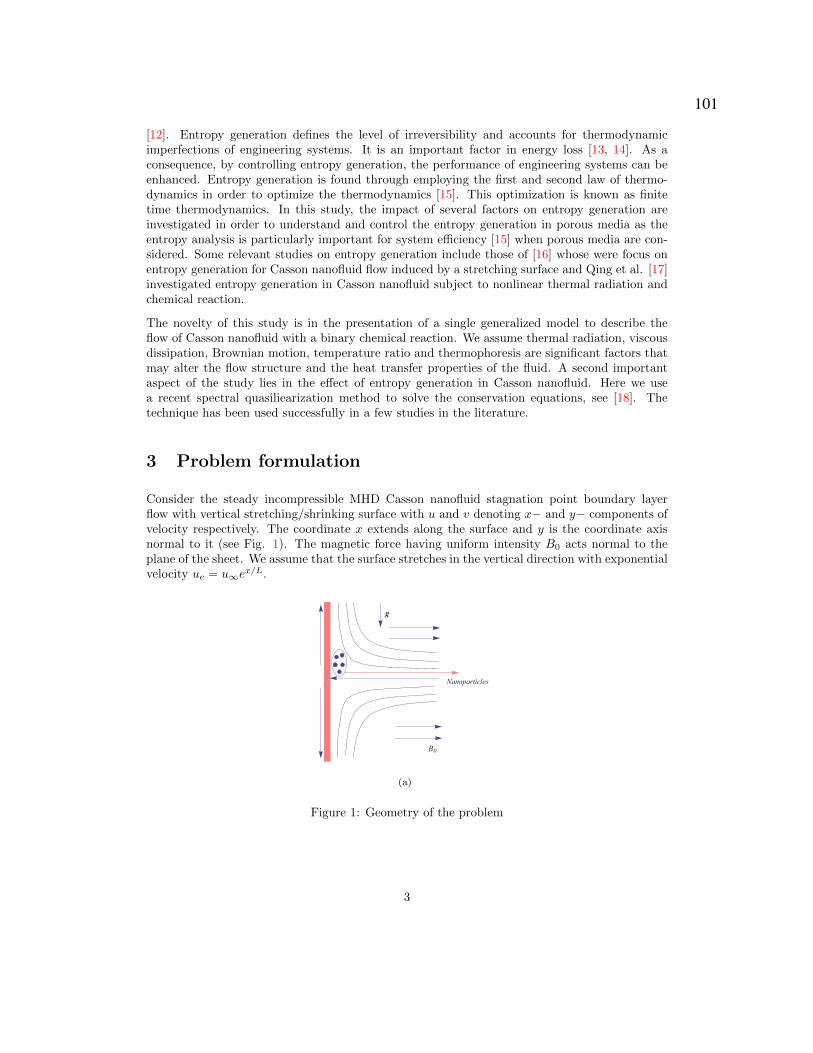
[12]. Entropy generation defines the level of irreversibility and accounts for thermodynamicimperfections of engineering systems. It is an important factor in energy loss [13, 14]. As aconsequence, by controlling entropy generation, the performance of engineering systems can beenhanced. Entropy generation is found through employing the first and second law of thermo-dynamics in order to optimize the thermodynamics [15]. This optimization is known as finitetime thermodynamics. In this study, the impact of several factors on entropy generation areinvestigated in order to understand and control the entropy generation in porous media as theentropy analysis is particularly important for system efficiency [15] when porous media are con-sidered. Some relevant studies on entropy generation include those of [16] whose were focus onentropy generation for Casson nanofluid flow induced by a stretching surface and Qing et al. [17]investigated entropy generation in Casson nanofluid subject to nonlinear thermal radiation andchemical reaction.

The novelty of this study is in the presentation of a single generalized model to describe theflow of Casson nanofluid with a binary chemical reaction. We assume thermal radiation, viscousdissipation, Brownian motion, temperature ratio and thermophoresis are significant factors thatmay alter the flow structure and the heat transfer properties of the fluid. A second importantaspect of the study lies in the effect of entropy generation in Casson nanofluid. Here we usea recent spectral quasiliearization method to solve the conservation equations, see [18]. Thetechnique has been used successfully in a few studies in the literature.

3 Problem formulation

Consider the steady incompressible MHD Casson nanofluid stagnation point boundary layerflow with vertical stretching/shrinking surface with u and v denoting x− and y− components ofvelocity respectively. The coordinate x extends along the surface and y is the coordinate axisnormal to it (see Fig. 1). The magnetic force having uniform intensity B0 acts normal to theplane of the sheet. We assume that the surface stretches in the vertical direction with exponentialvelocity ue = u∞ex/L.

0

B0

g

Nanoparticles

.

(a)

Figure 1: Geometry of the problem

3

101

The equations of the MHD Casson nanofluid model can be written as

∂u

∂x+∂v

∂y= 0, (3.1)

u∂u

∂x+ v

∂u

∂y= ν

(1 +

1

β

)∂2u∂y2

+σB2

0

ρ+ ue

∂ue∂x

+εµeffρk1

(ue − u)

+ g(Bt(T − T∞) +Bc(C − C∞)

), (3.2)

u∂T

∂x+ v

∂T

∂y= α

∂2T

∂y2+

16σ∗

3k∗(ρcp)f

∂

∂y

(T 3 ∂T

∂y

)+ν

cp

(1 +

1

β

)(∂u∂y

)2

+ τ

(DB

∂T

∂y

∂C

∂y+DT

T∞

(∂T∂y

)2), (3.3)

u∂C

∂x+ v

∂C

∂y= DB

∂2C

∂y2+DT

T∞

∂2T

∂y2− k2T

( T

T∞

)me(−Ea/kT )(C − C∞), (3.4)

where ν is the kinematic viscosity which represents the ratio of the dynamic viscosity µ to thedensity of the fluid ρ, β is the Casson parameter, σ and B2

0 are the electrical conductivity andthe strength of the magnetic field respectively, ue(x) is the external velocity, k1 is permeability ofthe porous medium, g is the acceleration, βt and βc are the thermal expansion and the expansionwith concentration respectively, T is the temperature, C is the concentration, α = (kf/ρcp) isthe thermal diffusion which represents the ratio between the effective thermal conductivity andthe effective specific heat, σ∗ and k∗ are the steaffan-Boltzman constant and mean absorption co-efficient respectively, (ρcp)f is the specific heat of the base fluid, DB is the Brownian motion, DT

is the thermophoretic diffusion. Moreover, k2T is the chemical reaction, (T/T∞)me(−Ea/kT ) is themodified Arrhenius function, in which k is the Boltzmann and m is the constant where −1<m<1

The auxiliary conditions for this study are

v = vw = vw0ex/2L, T = Tw(x), C = Cw(x), µ

∂u

∂y= σT

∂T

∂x+ σC

∂C

∂xat y = 0

u = ue(x) = u∞ex/L, T = T∞(x), C = C∞(x) at y →∞, (3.5)

where vw and ue are the velocities at the wall and at the outer edge of the boundary layer respec-tively, and L is the stretching velocity. Moreover, the emperature distribution and concentrationdistribution are defined as respectively

ue = u0ex/L, Tw(x) = T∞ + (T0 − T∞)ex/2L,

Cw(x) = C∞ + (C0 − C∞)ex/2L, (3.6)

where u0 is velocity parameter of the sheet, T0 and C0 are the temperature and concentrationdistributions in the stretching sheet respectively.

Equations (3.1)–(3.4) are converted into the couple of ordinary differential equations by usingthe following non-dimensional variable (see [19])

ψ =√

2νRe1/2ex/2Lf(η), η =

√Re

2

y

Lex/2L,

T = T∞ + (T0 − T∞)ex/2Lθ(η), C = C∞ + (C0 − C∞)ex/2Lφ(η). (3.7)

4

102

The system of Equations (3.1)–(3.4) become as

(1 +

1

β

)f ′′′ + ff ′′ − 2f ′

2

+ 2Rie(−3ξ/2)(θ +Nφ) + 2e−ξ(M2 + κp)(1− f ′) + 2 = 0,

(3.8)

1

Prθ′′ + θ′f − f ′θ + e(ξ/2)

(Nbθ′φ′ +Ntθ′

2)

+ Ec(

1 +1

β

)e(3ξ/2)f ′′

2

+Rd

(1 + (θf − 1)e(ξ/2)θ

)3θ′′ + 3(θf − 1)e(ξ/2)θ′

2

= 0, (3.9)

1

Leφ′′ + fφ′ − f ′φ+

1

Le

Nt

Nbθ′′ − σe(−ξ)

(1 + (θf − 1)e(ξ/2)θ

)me

(−E

1+(θf−1)e(ξ/2)θ

)φ = 0,

(3.10)

with boundary conditions

f(0) = s, f ′′(0) = 1− ε, θ(0) = 1, φ(0) = 1,

f ′(∞) = 1, θ(∞) = 0, φ(∞) = 0, (3.11)

where the prime denotes differentiation is with respect to η, Gr = gBt∆TL3/ν2 is the Grashof

number, Ri = Gr/Re2 is the Richardson number where Re = u0L/ν is the Reynolds number,ξ = x/L is the non-dimensional number along x-axis, N = Bc∆C/Bt∆T is the buoyancy param-eter, M2 = σB2

0L2/ρνRe is the magnetic parameter, κp = εµeffL

2/k1Reν is the permeabilityparameter, Pr = ν/α is the Prandtl number, Nb = τDB∆C/ν is the Brownian motion param-eter, Nt = τDT∆T/νT∞ is the Thermophoresis parameter, Ec = ν2Re2/∆TL2cp is the Eckertnumber, Rd = 16σ∗T 3

∞/3ν(ρcp)fk∗ is the radiation parameter, θf = Tf/T∞ is the tempera-

ture ratio, Le = ν/DB is the Lewis number, E = /Ea/kT∞ binary chemical reaction rate andσ = 2k2TL

2/Reν. In Equation (3.11), s = −vw0

√2L/ν

√Re is the suction/ injection parameter

where s>0 is suction and s<0 is injection and ε = MaC/MaT = σC∆C/σT∆T is the Marangoniparameter, where MaC and MaT are the solutal Marangoni number and thermal Marangoninumber respectively (see [20]).The local Nusselt number Nu and the local Sherwood number Sh are defined as

Nu =xhw

kf (Tw − T∞), Sh =

xhmρDB(Cw − C∞)

, (3.12)

where the heat flux hw and the mass flux hm at the wall are given as

hw = −kf[∂T

∂y

]

y=0

, hm = −ρDB

[∂C

∂y.

]

y=0

(3.13)

Using variables in equation (3.7) and Equation (3.13), we get from equation (3.12)

√2Re−1/2Nu = −

[1 +Nd(1 + (θf − 1))3eξ/2

]eξξθ′(0),

√2Re−1/2Sh = −ξeξφ′(0), (3.14)

where Re = u0Lν is the local Reynolds number.

5

103

4 Entropy Generation

Entropy generation is dependent on the reversibility of a particular process. For an isolatedsystem entropy tends to increase with time, but remains constant for reversible reactions. Withan increase in use of nanofluids and nanoparticles in engineering and medical applications, it isimportant to study and understand the impact of these nanoparticles on entropy generation onreal devices, [14]. The volumetric rate of local entropy generation for the nanofluid according tothe second law of thermodynamics, is given for two-dimensional flow as

S′′′gen =kfT 2∞

((∂T∂y

)2+

16σ∗T 3

3kfk∗

(∂T∂y

)2)+

µ

T∞

(1 +

1

β

)(∂u∂y

)2

+σB2

0

T∞u2 +

µ

T∞k1u2

+µ

k1u2 +

RD

C∞

(∂C

∂y

)2

+RD

T∞

(∂T∂y

∂C

∂y

). (4.1)

Equation (4.3) shows that entropy generation has several components . The first source is causedby the heat transfer through the thermal radiation; the second is caused by viscous dissipation;the third and fourth are caused by the magnetic field and mean absorption coefficient respectively;the last two sources are caused by mass transfer.It is appropriate to obtain the entropy generation number as a ratio between the the localvolumetric entropy generation S′′′gen and a characteristic rate of entropy generation S′′′0 such thatS′′′0 is written as [12]

S′′′0 =kf (Tw − T∞)2

L2T 2∞. (4.2)

The characteristic entropy generation rate S′′′0 is the optimal entropy generation at which thethermodynamic performance of a system is optimized [21]. Finding S′′′0 requires solving anoptimization problem which is constrained by the irreversible operations of the system. Thephysical characteristics of the system are varied until minimum entropy generation is foundBejan [21].

The entropy generation number can be expressed as

NG =S′′′genS′′′0

=1

2

[1 +Rd

(1 + (θf − 1)θ

)3]Ree2ξθ′

2

+1

2

(1 +

1

β

) ReBr

(θf − 1)2eξf ′′

2

+

ReΣΩ2

2(θf − 1)2e2ξφ′

2

+ReBr

(θf − 1)2

(M2 + κp

)f ′

2

+ReΩΣ

2(θf − 1)e2ξθ′φ′, (4.3)

where Br, Σ and Ω the Brinkman number, a constant parameter and the concentration differencerespectively. These parameters are expressed as:

Br =µuw(x)2

T∞kf, Σ =

C∞RDkf

, Ω =C0 − C∞C∞

. (4.4)

5 Method of solution

The quasi-linearization method (QLM) is a generalization of the Newton-Raphson method (Bell-man and Kalaba [22]). The nonlinear equations are linearized using a Taylor series assumingthat the difference between the current iteration, r+1, and the previous iteration, r is negligible.

6

104

Applying the quasi-linearization method to Equations (3.8)–(3.10) and (3.11), gives the followingiterative schemes:

a0,rf′′′r+1 + a1,rf

′′r+1 + a2,rf

′r+1 + a3,rfr+1 + a4,rθr+1 + a5,rφr+1 = Rf , (5.1)

b0,rθ′′r+1 + b1,rθ

′r+1 + b2,rθr+1 + b3,rfr+1 + b4,rf

′r+1 + b5,rf

′′r+1 + b6,rφ

′r+1 = Rθ, (5.2)

c0,rφ′′r+1 + c1,rφ

′r+1 + c2,rφr+1 + c3,rfr+1 + c4,rf

′r+1 + c5,rθr+1 + c6,rθ

′′r+1 = Rφ, (5.3)

subject to

fr+1(0) = s, f ′′r+1(0) = 1− ε, θr+1(0) = 1, φr+1(0) = 1,

f ′r+1(∞) = 1, θr+1(∞) = 0, φr+1(∞) = 0. (5.4)

The coefficients in Equations (5.1)–(5.3) are

a0,r = 1 +1

β, a1,r = fr, a2,r = −4f ′r − 2e−ξ(M2 + κp), a3,r = f ′′r ,

a4,r = 2Rie(−3ξ/2), a5,r = 2NRie(−3ξ/2), (5.5)

b0,r =1

Pr+Rd

(1 + (θf − 1)e(ξ/2)θr

)3

,

b1,r = fr + e(ξ/2)(Nbφ′r + 2Ntθ′r

)+ 6Rd(θf − 1)e(ξ/2)θ′r,

b2,r = −f ′r + 3Rd(

1 + (θf − 1)eξ/2θr

)2θ′′r (θf − 1)e(ξ/2), b3,r = θ′r, b4,r = −θr,

b5,r = 2Ec(

1 +1

β

)e(3ξ/2)f ′′r , b6,r = eξ/2Nbθ′r, (5.6)

c0,r = 1, c1,r = Lefr, c2,r = −Lef ′r − Leσe−ξ(

1 + (θf − 1)e(ξ/2)θr

)me−E/1+(θf−1)eξ/2θr ,

c3,r = Leφ′r, c4,r = −Leφr, c6,r =Nt

Nb,

c5,r = −σφre−ξ(

1 + (θf − 1)eξ/2θr

)me(−E/1+(θf−1)eξ/2θr) E(θf − 1)eξ/2

(1 + (θf − 1)eξ/2θr

)2

+me(−E/1+(θf−1)eξ/2θr)(1 + (θf − 1)eξ/2θr)m−1

(θf − 1)eξ/2

(5.7)

Equations (5.1)–(5.3) were solved using the Chebyshev pseudo-spectral method with the Gauss-Lobatto points [23]

xi = cos(πiN

), i = 0, 1, 2, . . . , N − 1 ≤ xi ≥ 1, (5.8)

where N is the number of collocation points. A linear transformation formula was used totransfer the interval [0, L] to the [−1, 1] , where L represents the boundary condition at infinity.

The derivatives with respect to η are expressed is terms of the Chebyshev differentiation matrixsuch as

df(p)r

dηp

∣∣∣∣η=ηj

=N∑

k=0

Djkf(ηk) = DF, j = 1, 2, . . . , N, (5.9)

7

105

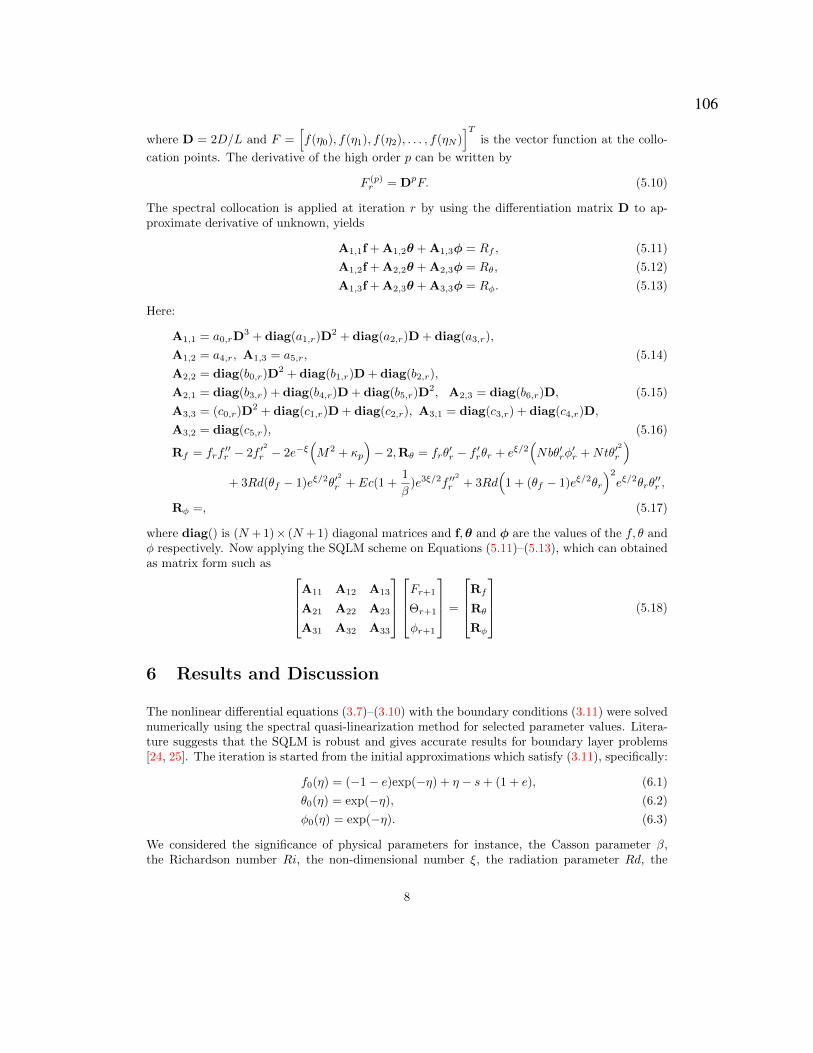
where D = 2D/L and F =[f(η0), f(η1), f(η2), . . . , f(ηN )

]Tis the vector function at the collo-

cation points. The derivative of the high order p can be written by

F (p)r = DpF. (5.10)

The spectral collocation is applied at iteration r by using the differentiation matrix D to ap-proximate derivative of unknown, yields

A1,1f + A1,2θ + A1,3φ = Rf , (5.11)

A1,2f + A2,2θ + A2,3φ = Rθ, (5.12)

A1,3f + A2,3θ + A3,3φ = Rφ. (5.13)

Here:

A1,1 = a0,rD3 + diag(a1,r)D

2 + diag(a2,r)D + diag(a3,r),

A1,2 = a4,r, A1,3 = a5,r, (5.14)

A2,2 = diag(b0,r)D2 + diag(b1,r)D + diag(b2,r),

A2,1 = diag(b3,r) + diag(b4,r)D + diag(b5,r)D2, A2,3 = diag(b6,r)D, (5.15)

A3,3 = (c0,r)D2 + diag(c1,r)D + diag(c2,r), A3,1 = diag(c3,r) + diag(c4,r)D,

A3,2 = diag(c5,r), (5.16)

Rf = frf′′r − 2f ′

2

r − 2e−ξ(M2 + κp

)− 2,Rθ = frθ

′r − f ′rθr + eξ/2

(Nbθ′rφ

′r +Ntθ′

2

r

)

+ 3Rd(θf − 1)eξ/2θ′2

r + Ec(1 +1

β)e3ξ/2f ′′

2

r + 3Rd(

1 + (θf − 1)eξ/2θr

)2eξ/2θrθ

′′r ,

Rφ =, (5.17)

where diag() is (N + 1)× (N + 1) diagonal matrices and f,θ and φ are the values of the f, θ andφ respectively. Now applying the SQLM scheme on Equations (5.11)–(5.13), which can obtainedas matrix form such as

A11 A12 A13

A21 A22 A23

A31 A32 A33

Fr+1

Θr+1

φr+1

=

Rf

Rθ

Rφ

(5.18)

6 Results and Discussion

The nonlinear differential equations (3.7)–(3.10) with the boundary conditions (3.11) were solvednumerically using the spectral quasi-linearization method for selected parameter values. Litera-ture suggests that the SQLM is robust and gives accurate results for boundary layer problems[24, 25]. The iteration is started from the initial approximations which satisfy (3.11), specifically:

f0(η) = (−1− e)exp(−η) + η − s+ (1 + e), (6.1)

θ0(η) = exp(−η), (6.2)

φ0(η) = exp(−η). (6.3)

We considered the significance of physical parameters for instance, the Casson parameter β,the Richardson number Ri, the non-dimensional number ξ, the radiation parameter Rd, the

8

106

temperature ratio θf and the binary chemical reaction rate E on the velocity profiles f ′(η), θ(η)the temperature profiles and the concentration profiles φ(η). The values of Ri and ξ are 0.1and 1.2 respectively, which are determined from [19]. However, the rest of the other parametersPr = 6.7, Le = 4, Nt = 10−3, β = 2 e = 1, s = 2, κp = 0.6, E = 0.5, Rd = 0.15, θf = 2,Nb = 0.5, Ec = 0.3, σ = 1, m = 0.5, M = 0.5, N = 0.5 [19, 20].

The variation in the local Nusselt number and the Sherwood number for various values of theCasson parameter, Richardson number, the radiation parameter, the temperature ratio and thenon-dimensional number are provided in Table 1. We note that the Nusselt number increases asCasson parameter β increases, while the Sherwood number decrease with increasing with otherparameters fixed. It is also observed that the Nusselt number reduces as Richardson number Riincreases, whereas the Sherwood number increase. The Nusselt number and Sherwood numberare vary positively with Rd. The same result it is seen with respect to the temperature ratio.The Nusselt number and Sherwood number vary inversely with the non-dimensional number.

Table 1: Numerical values of −θ′(0) and −φ′(0) with different values of β,Ri,Rd, θf and ξ whenPr = 6.7, Le = 4, Nt = 10−3, e = 1, s = 2, κp = 0.6, E = 0.5, Nb = 0.5, Ec = 0.3, σ = 1,m = 0.5, M = 0.5, N = 0.5

β Ri Rd θf ξ Re−1/2Nu Re−1/2Sh

1 −0.89826777 1.39934551

3 0.1 0.15 2 1.2 −0.18205046 1.27881276

5 −0.09225992 1.26745514

0.5 −0.47888070 1.49772170

2 1 0.15 2 1.2 −0.76012804 1.72149615

1.5 −1.05219374 1.90147611

0.5 0.04856763 1.27101508

2 0.1 1 2 1.2 0.15337722 1.27337443

1.5 0.16035341 1.27345065

1.01 −2.03641215 1.18001097

2 0.1 1.5 1.3 1.2 −0.73187093 1.24466801

3 −0.17183036 1.32679920

0.5 −0.17620748 1.59246412

2 0.1 0.15 2 1.5 −0.45415417 1.24508669

2.5 −1.00665598 1.12749275

Figs. 2(a)–(c) show the effect of the Casson parameter β on the fluid velocity, temperatureand concentration profiles. In Figs. 2(a) and (b), we observe that the velocity profiles and thetemperature profiles decrease as the Casson parameter increases. From Fig. 2(c), it is notedthat the Casson parameter is an increasing function of the concentration profiles. For very largevalues of the Casson parameter, i.e. β →∞, the fluid becomes Newtonian.

The variation of velocity, temperature and concentration profiles with the mixed convectionparameter Ri are depicted in Fig. 3(a)–(c), respectively. From Figs. 3(a)–(b), it is observed

9

107

that the effect of increasing the mixed convection parameter is to increase the velocity and thetemperature profiles. When Ri increase, the bouyancy influences increase and subsequentlythe acceleration of the fluid flow increases. For the temperature profiles, as Ri increases, theconvection cooling effect reduces such that the temperature increases. It is also note that fromFig. 3(b) the temperature profiles increase when 0 ≤ η ≤ 1.5 while η>1.5, the temperatureprofiles decrease and hence becomes constant far from the stretching sheet. Fig. 3(c) revealsthat the concentration profiles of the fluid decreases as the mixed convection parameter increases.

Figs. 4(a)–(b) show the velocity, temperature and concentration profiles for different non-dimensional number ξ. It is observed from Fig. 4(a) that the velocity profiles decrease withincrease in the non-dimensional number in the momentum boundary layer. In Fig. 4(b) thethermal layer thickness increases as the non-dimensional number increases significantly near thestretching sheet. Furthermore, the same result also holds for the concentration profiles Fig. 4(c).

The effects of the thermal radiation parameter on the temperature profiles is shown in Fig. 5(a).It is observed that the temperature increases as thermal radiation increases, which is consistentwith physical observations regarding to the affect of increasing thermal radiation.

Figs. 6(a)–(b) show the behaviour of temperature and concentration profiles for different valuesof temperature ratio θf . It is observed that an increase in the value of temperature ratio leads toan decrease of the temperature and concentration profiles. It is also obtained from Fig. 6(a) thatincrease in the values of temperature ratio leads to decrease in the temperature profiles close thevalues of 0 ≤ η ≤ 1.5 whereas reverse trend is observed away from the sheet for η>1.5

The changes in the concentration profiles with binary chemical reaction rate E is depicted inFig. 7(a). It is noted that increasing the binary chemical reaction rate trends to increases in theconcentration profiles since binary chemical reaction rate enhances the concentration of species.

The variations of the local Nusselt number and local Sherwood number with the magnetic pa-rameter for different values of Casson parameter β are depicted in Figs. 8(a) and (b) respectively.It is noted that the influence of increasing the magnetic field is to increase the Nusselt numberwhich it is reduce for all values of Casson parameter β. Moreover, the magnetic filed and Cassonparameter are varying inversely with the Sherwood number.

In the following, entropy generation is discussed which is an important attribute of the flow. Theentropy generation is influenced by the quantum and changes in the physical characteristics ofthe fluid and the porous medium as can be seen in equation (4.3). We consider how physicalparameters such as non-dimensional number ξ the permeability parameter κp, the Reynoldsnumber Re, the temperature ratio θf and Casson parameter β influence entropy generation.

The influence of varying the non-dimensional number, the permeability parameter and theReynolds number on entropy generation are depicted in Figs. 9(a), (b) and (c) respectively.An increase in the non-dimensional number causes an increase in entropy generation. A reduc-tion in entropy generation is noted with an increase in κp as depicted in Fig. 9(b) close the values0 ≤ η ≤ 0.5 while reverse result is observed on the range is no far way from the sheet η>0.5.Fig. 9(c) illustrates the influence of Reynolds number on entropy generation. In alignment withequation (4.3), it is observed that the entropy generation increases in a response to the increasein Reynolds numbe. The physical interpretation of this observation is the increase of fluid frictionand heat transfer due to the change in the structure of the flow which may be attributed to theincrease in Reynolds number.

Figs. 10(a) and (b) show the effect of different values of temperature ratio and Casson parameter

10

108

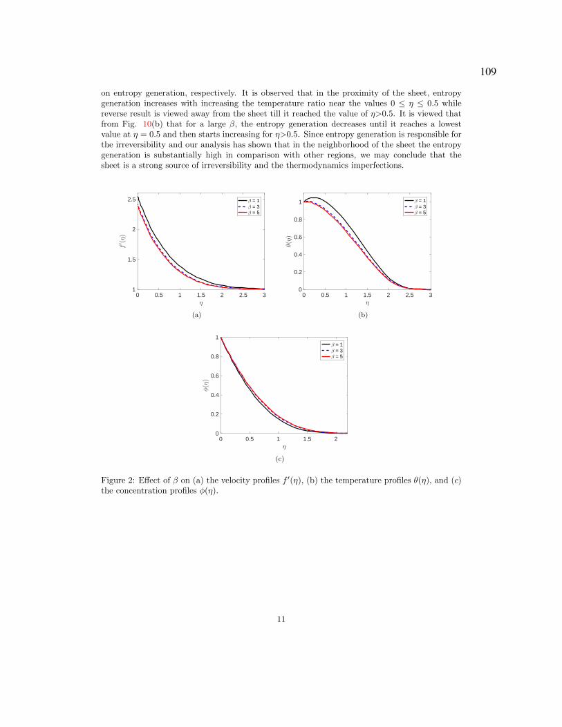
on entropy generation, respectively. It is observed that in the proximity of the sheet, entropygeneration increases with increasing the temperature ratio near the values 0 ≤ η ≤ 0.5 whilereverse result is viewed away from the sheet till it reached the value of η>0.5. It is viewed thatfrom Fig. 10(b) that for a large β, the entropy generation decreases until it reaches a lowestvalue at η = 0.5 and then starts increasing for η>0.5. Since entropy generation is responsible forthe irreversibility and our analysis has shown that in the neighborhood of the sheet the entropygeneration is substantially high in comparison with other regions, we may conclude that thesheet is a strong source of irreversibility and the thermodynamics imperfections.

0 0.5 1 1.5 2 2.5 3η

1

1.5

2

2.5

f′ (η)

β = 1β = 3β = 5

(a)

0 0.5 1 1.5 2 2.5 3η

0

0.2

0.4

0.6

0.8

1

θ(η)

β = 1β = 3β = 5

(b)

0 0.5 1 1.5 2η

0

0.2

0.4

0.6

0.8

1

φ(η)

β = 1β = 3β = 5

(c)

Figure 2: Effect of β on (a) the velocity profiles f ′(η), (b) the temperature profiles θ(η), and (c)the concentration profiles φ(η).

11

109

0 0.5 1 1.5 2 2.5η

1

1.5

2

2.5

3

3.5

f′ (η)

Ri = 0.5Ri = 1Ri = 1.5

(a)

0 0.5 1 1.5 2 2.5η

0

0.2

0.4

0.6

0.8

1

1.2

θ(η)

Ri = 0.5Ri = 1Ri = 1.5

(b)

0 0.5 1 1.5η

0

0.2

0.4

0.6

0.8

1

φ(η)

Ri = 0.5Ri = 1Ri = 1.5

(c)

Figure 3: Effect of Ri on (a) the velocity profiles f ′(η), (b) the temperature profiles θ(η), and(c) the concentration profiles φ(η).

12

110

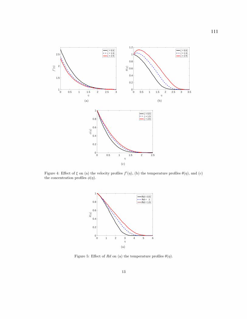
0 0.5 1 1.5 2 2.5 3η

1

1.5

2

2.5f′ (η)

ξ = 0.5ξ = 1.5ξ = 2.5

(a)

0 0.5 1 1.5 2 2.5 3 3.5η

0

0.2

0.4

0.6

0.8

1

1.2

θ(η)

ξ = 0.5ξ = 1.5ξ = 2.5

(b)

0 0.5 1 1.5 2 2.5η

0

0.2

0.4

0.6

0.8

1

φ(η)

ξ = 0.5ξ = 1.5ξ = 2.5

(c)

Figure 4: Effect of ξ on (a) the velocity profiles f ′(η), (b) the temperature profiles θ(η), and (c)the concentration profiles φ(η).

0 1 2 3 4 5 6η

0

0.2

0.4

0.6

0.8

1

θ(η)

Rd = 0.5Rd = 1Rd = 1.5

(a)

Figure 5: Effect of Rd on (a) the temperature profiles θ(η).

13

111

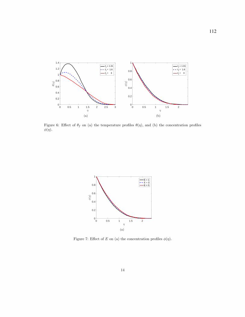
0 0.5 1 1.5 2 2.5 3η

0

0.2

0.4

0.6

0.8

1

1.2

1.4

θ(η)

θf = 1.01

θf = 1.6

θf = 3

(a)

0 0.5 1 1.5 2η

0

0.2

0.4

0.6

0.8

1

φ(η)

θf = 1.01

θf = 1.6

θf = 3

(b)

Figure 6: Effect of θf on (a) the temperature profiles θ(η), and (b) the concentration profilesφ(η).

0 0.5 1 1.5 2η

0

0.2

0.4

0.6

0.8

1

φ(η)

E = 1E = 3E = 5

(a)

Figure 7: Effect of E on (a) the concentration profiles φ(η).

14

112

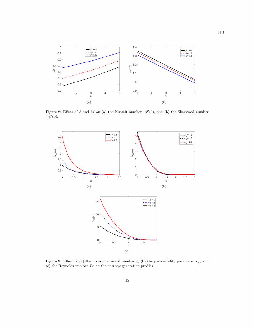
1 2 3 4 5M

-0.7

-0.6

-0.5

-0.4

-0.3

-0.2

-0.1

0

−θ′ (0)

β= 0.8β= 1β= 1.5

(a)

1 2 3 4 5M

0.9

1

1.1

1.2

1.3

1.4

−φ′ (0)

β = 0.8β = 1β = 1.5

(b)

Figure 8: Effect of β and M on (a) the Nusselt number −θ′(0), and (b) the Sherwood number−φ′(0).

0 0.5 1 1.5 2 2.5η

0.5

1

1.5

2

2.5

3

3.5

4

NG(η)

ξ = 0.5ξ = 1.5ξ = 2.5

(a)

0 0.5 1 1.5 2 2.5 3η

0

1

2

3

4

5N

G(η)

κp = 1

κp = 2

κp = 2.8

(b)

0 0.5 1 1.5 2η

0

5

10

15

NG(η)

Re = 1Re = 2Re = 3

(c)

Figure 9: Effect of (a) the non-dimensional number ξ, (b) the permeability parameter κp, and(c) the Reynolds number Re on the entropy generation profiles.

15

113

0 0.5 1 1.5 2η

0

1

2

3

4

5

NG(η)

θf = 1.01

θf = 1.6

θf = 3

(a)

0 0.5 1 1.5 2η

0

1

2

3

4

5

6

NG(η)

β = 1β = 3β = 5

(b)

Figure 10: Effect of (a) the temperature ratio parameter θf , and (b) the Casson parameter β onthe entropy generation profiles.

16

114

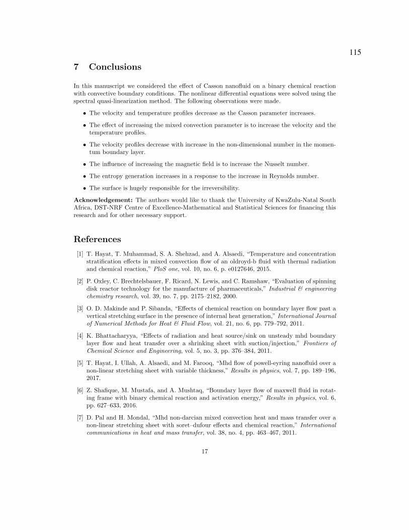
7 Conclusions

In this manuscript we considered the effect of Casson nanofluid on a binary chemical reactionwith convective boundary conditions. The nonlinear differential equations were solved using thespectral quasi-linearization method. The following observations were made.

• The velocity and temperature profiles decrease as the Casson parameter increases.

• The effect of increasing the mixed convection parameter is to increase the velocity and thetemperature profiles.

• The velocity profiles decrease with increase in the non-dimensional number in the momen-tum boundary layer.

• The influence of increasing the magnetic field is to increase the Nusselt number.

• The entropy generation increases in a response to the increase in Reynolds number.

• The surface is hugely responsible for the irreversibility.

Acknowledgement: The authors would like to thank the University of KwaZulu-Natal SouthAfrica, DST-NRF Centre of Excellence-Mathematical and Statistical Sciences for financing thisresearch and for other necessary support.

References

[1] T. Hayat, T. Muhammad, S. A. Shehzad, and A. Alsaedi, “Temperature and concentrationstratification effects in mixed convection flow of an oldroyd-b fluid with thermal radiationand chemical reaction,” PloS one, vol. 10, no. 6, p. e0127646, 2015.

[2] P. Oxley, C. Brechtelsbauer, F. Ricard, N. Lewis, and C. Ramshaw, “Evaluation of spinningdisk reactor technology for the manufacture of pharmaceuticals,” Industrial & engineeringchemistry research, vol. 39, no. 7, pp. 2175–2182, 2000.

[3] O. D. Makinde and P. Sibanda, “Effects of chemical reaction on boundary layer flow past avertical stretching surface in the presence of internal heat generation,” International Journalof Numerical Methods for Heat & Fluid Flow, vol. 21, no. 6, pp. 779–792, 2011.

[4] K. Bhattacharyya, “Effects of radiation and heat source/sink on unsteady mhd boundarylayer flow and heat transfer over a shrinking sheet with suction/injection,” Frontiers ofChemical Science and Engineering, vol. 5, no. 3, pp. 376–384, 2011.

[5] T. Hayat, I. Ullah, A. Alsaedi, and M. Farooq, “Mhd flow of powell-eyring nanofluid over anon-linear stretching sheet with variable thickness,” Results in physics, vol. 7, pp. 189–196,2017.

[6] Z. Shafique, M. Mustafa, and A. Mushtaq, “Boundary layer flow of maxwell fluid in rotat-ing frame with binary chemical reaction and activation energy,” Results in physics, vol. 6,pp. 627–633, 2016.

[7] D. Pal and H. Mondal, “Mhd non-darcian mixed convection heat and mass transfer over anon-linear stretching sheet with soret–dufour effects and chemical reaction,” Internationalcommunications in heat and mass transfer, vol. 38, no. 4, pp. 463–467, 2011.

17

115

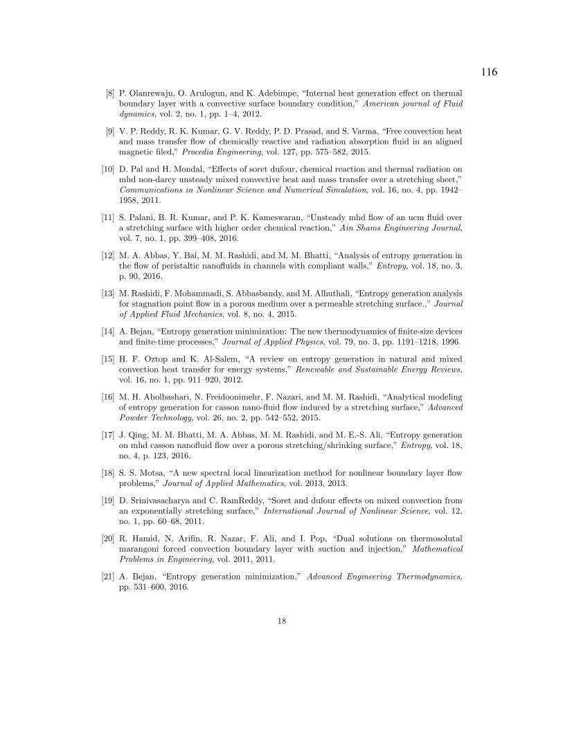
[8] P. Olanrewaju, O. Arulogun, and K. Adebimpe, “Internal heat generation effect on thermalboundary layer with a convective surface boundary condition,” American journal of Fluiddynamics, vol. 2, no. 1, pp. 1–4, 2012.

[9] V. P. Reddy, R. K. Kumar, G. V. Reddy, P. D. Prasad, and S. Varma, “Free convection heatand mass transfer flow of chemically reactive and radiation absorption fluid in an alignedmagnetic filed,” Procedia Engineering, vol. 127, pp. 575–582, 2015.

[10] D. Pal and H. Mondal, “Effects of soret dufour, chemical reaction and thermal radiation onmhd non-darcy unsteady mixed convective heat and mass transfer over a stretching sheet,”Communications in Nonlinear Science and Numerical Simulation, vol. 16, no. 4, pp. 1942–1958, 2011.

[11] S. Palani, B. R. Kumar, and P. K. Kameswaran, “Unsteady mhd flow of an ucm fluid overa stretching surface with higher order chemical reaction,” Ain Shams Engineering Journal,vol. 7, no. 1, pp. 399–408, 2016.

[12] M. A. Abbas, Y. Bai, M. M. Rashidi, and M. M. Bhatti, “Analysis of entropy generation inthe flow of peristaltic nanofluids in channels with compliant walls,” Entropy, vol. 18, no. 3,p. 90, 2016.

[13] M. Rashidi, F. Mohammadi, S. Abbasbandy, and M. Alhuthali, “Entropy generation analysisfor stagnation point flow in a porous medium over a permeable stretching surface.,” Journalof Applied Fluid Mechanics, vol. 8, no. 4, 2015.

[14] A. Bejan, “Entropy generation minimization: The new thermodynamics of finite-size devicesand finite-time processes,” Journal of Applied Physics, vol. 79, no. 3, pp. 1191–1218, 1996.

[15] H. F. Oztop and K. Al-Salem, “A review on entropy generation in natural and mixedconvection heat transfer for energy systems,” Renewable and Sustainable Energy Reviews,vol. 16, no. 1, pp. 911–920, 2012.

[16] M. H. Abolbashari, N. Freidoonimehr, F. Nazari, and M. M. Rashidi, “Analytical modelingof entropy generation for casson nano-fluid flow induced by a stretching surface,” AdvancedPowder Technology, vol. 26, no. 2, pp. 542–552, 2015.

[17] J. Qing, M. M. Bhatti, M. A. Abbas, M. M. Rashidi, and M. E.-S. Ali, “Entropy generationon mhd casson nanofluid flow over a porous stretching/shrinking surface,” Entropy, vol. 18,no. 4, p. 123, 2016.

[18] S. S. Motsa, “A new spectral local linearization method for nonlinear boundary layer flowproblems,” Journal of Applied Mathematics, vol. 2013, 2013.

[19] D. Srinivasacharya and C. RamReddy, “Soret and dufour effects on mixed convection froman exponentially stretching surface,” International Journal of Nonlinear Science, vol. 12,no. 1, pp. 60–68, 2011.

[20] R. Hamid, N. Arifin, R. Nazar, F. Ali, and I. Pop, “Dual solutions on thermosolutalmarangoni forced convection boundary layer with suction and injection,” MathematicalProblems in Engineering, vol. 2011, 2011.

[21] A. Bejan, “Entropy generation minimization,” Advanced Engineering Thermodynamics,pp. 531–600, 2016.

18

116

[22] R. E. Bellman and R. E. Kalaba, “Quasilinearization and nonlinear boundary-value prob-lems,” 1965.

[23] T. Agbaje, S. Mondal, Z. Makukula, S. Motsa, and P. Sibanda, “A new numerical approachto mhd stagnation point flow and heat transfer towards a stretching sheet,” Ain ShamsEngineering Journal, 2016.

[24] S. Motsa, P. Sibanda, and S. Shateyi, “On a new quasi-linearization method for systems ofnonlinear boundary value problems,” Mathematical Methods in the Applied Sciences, vol. 34,no. 11, pp. 1406–1413, 2011.

[25] M. Almakki, S. Dey, S. Mondal, and P. Sibanda, “On unsteady three-dimensional axisym-metric mhd nanofluid flow with entropy generation and thermo-diffusion effects on a non-linear stretching sheet,” Entropy, vol. 19, no. 7, p. 168, 2017.

19

117

Chapter 6

A model for entropy generation at stagnation

point flow of non-Newtonian Jeffrey, Maxwell

and Oldroyd-B nanofluids

In previous chapters, a model is developed to describe a particular non-Newtonian fluid which

might considered as a shortcoming from the perspective of generality. Further, we adapted a single

method to solve the model equations. In this chapter a general model that encapsulates different

types of non-Newtonian fluids is developed and solved using different solution methods.

In this chapter, we propose a single model for the steady laminar boundary-layer flow describing

the behavior of Jeffrey, Maxwell and Oldroyd-B nanofluids. The model is used to study entropy

generation, and heat and mass transfer near a stagnation point in the flow. The system of non-

linear equations is solved numerically using three different methods; namely a spectral relaxation

method, a spectral quasiliearization method and the spectral local linearization method. The resid-

ual errors is used to determine the most accurate solution method.

118

Received: 20 March 2018 | Accepted: 14 July 2018

DOI: 10.1002/htj.21366

OR IG INAL ART I C L E

Amodel for entropy generation in stagnation‐point flowof non‐Newtonian Jeffrey,Maxwell,and Oldroyd‐B nanofluids

Mohamed Almakki1 | Samir Kumar Nandy2 |Sabyasachi Mondal3 | Precious Sibanda1 | Dora Sibanda4

1School of Mathematics, Statistics andComputer Science, University ofKwaZulu‐Natal, Pietermaritzburg,South Africa2Department of Mathematics, A. K. P. C.Mahavidyalaya, Hooghly, India3Department of Mathematics, AmityUniversity, Kolkata, Newtown, India4School of Education, University ofKwaZulu‐Natal, Pinetown, South Africa

CorrespondenceSabyasachi Mondal, Department ofMathematics, Amity University, Kolkata,Newtown 700135, West Bengal, India.Email: sabya.mondal.2007@gmail.com

Abstract

We present a generalized model to describe the flow of

three non‐Newtonian nanofluids, namely, Jeffrey, Max-

well, and Oldroyd‐B nanofluids. Using this model, we

study entropy generation and heat transfer in laminar

nanofluid boundary‐layer stagnation‐point flow. The flow

is subject to an external magnetic field. The conventional

energy equation is modified by the incorporation of

nanoparticle Brownian motion and thermophoresis effects.

A hydrodynamic slip velocity is used in the initial

condition as a component of the stretching velocity. The

system of nonlinear equations is solved numerically using

three different methods, a spectral relaxation method,

spectral quasilinearization method, and the spectral local

linearization method, first to determine the most accurate

of these methods, and second as a measure to validate the

numerical simulations. The residual errors for each

method are presented. The numerical results show that

the spectral relaxation method is the most accurate of the

three methods, and this method is used subsequently to

solve the transport equations and thus to determine the

empirical impact of the physical parameters on the fluid

properties and entropy generation.

KEYWORD S

Brownian motion, entropy generation, non‐Newtonian nanofluids,

spectral methods, thermophoresis

Heat Transfer—Asian Res. 2019;48:24–41.wileyonlinelibrary.com/journal/htj24 | © 2018 Wiley Periodicals, Inc.

119

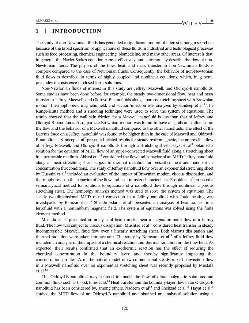
1 | INTRODUCTION

The study of non‐Newtonian fluids has generated a significant amount of interest among researchersbecause of the broad spectrum of applications of these fluids in industrial and technological processessuch as food processing, chemical engineering, biomedicine, and many other areas. Of interest is that,in general, the Navier‐Stokes equation cannot effectively, and substantially describe the flow of non‐Newtonian fluids. The physics of the flow, heat, and mass transfer in non‐Newtonian fluids iscomplex compared to the case of Newtonian fluids. Consequently, the behavior of non‐Newtonianfluid flows is described in terms of highly coupled and nonlinear equations, which, in general,precludes the existence of closed‐form solutions.

Non‐Newtonian fluids of interest in this study are Jeffrey, Maxwell, and Oldroyd‐B nanofluids.Some studies have been done before, for example, the steady two‐dimensional flow, heat and masstransfer in Jeffrey, Maxwell, and Oldroyd‐B nanofluids along a porous stretching sheet with Brownianmotion, thermophoresis, magnetic field, and suction/injection was analyzed by Sandeep et al.1 TheRunge‐Kutta method and a shooting technique were used to solve the system of equations. Theresults showed that the wall skin friction for a Maxwell nanofluid is less than that of Jeffrey andOldroyd‐B nanofluids. Also, particle Brownian motion was found to have a significant influence onthe flow and the behavior of a Maxwell nanofluid compared to the other nanofluids. The effect of theLorentz force on a Jeffrey nanofluid was found to be higher than in the case of Maxwell and Oldroyd‐B nanofluids. Sandeep et al2 presented related results for steady hydromagnetic, incompressible flowof Jeffrey, Maxwell, and Oldroyd‐B nanofluids through a stretching sheet. Hayat et al3 obtained asolution for the equation of MHD flow of an upper‐convected Maxwell fluid along a stretching sheetin a permeable medium. Abbasi et al4 considered the flow and behavior of an MHD Jeffrey nanofluidalong a linear stretching sheet subject to thermal radiation for prescribed heat and nanoparticleconcentration flux conditions. The study of Jeffrey nanofluid flow over an exponential stretching sheetby Hussain et al5 included an evaluation of the impact of Brownian motion, viscous dissipation, andthermophoresis on the behavior of the flow and heat transfer characteristics. Rashidi et al6 proposed asemianalytical method for solutions to equations of a nanofluid flow through nonlinear a porousstretching sheet. The homotopy analysis method was used to solve the system of equations. Thesteady two‐dimensional MHD mixed convection in a Jeffrey nanofluid with Joule heating wasinvestigated by Ramzan et al.7 Sheikholeslami et al8 presented an analysis of heat transfer in aferrofluid with a nonuniform magnetic field. The system of equations was solved using the finiteelement method.

Mustafa et al9 presented an analysis of heat transfer near a stagnation‐point flow of a Jeffreyfluid. The flow was subject to viscous dissipation. Mushtaq et al10 considered heat transfer in steadyincompressible Maxwell fluid flow over a linearly stretching sheet. Both viscous dissipation andthermal radiation were taken into account. The study by Narayana et al11 of a Jeffrey fluid flowincluded an analysis of the impact of a chemical reaction and thermal radiation on the flow field. Asexpected, their results confirmed that an exothermic reaction has the effect of reducing thechemical concentration in the boundary layer, and thereby significantly impacting theconcentration profiles. A mathematical model of two‐dimensional steady mixed convection flowin a Maxwell nanofluid over an exponential stretching sheet was recently proposed by Mustafaet al.12

The Oldroyd‐B nanofluid may be used to model the flow of dilute polymeric solutions andcommon fluids such as blood, Pires et al.13 Heat transfer and the boundary‐layer flow in an Oldroyd‐Bnanofluid has been considered by, among others, Nadeem et al14 and Shehzad et al.15 Hayat et al16

studied the MHD flow of an Oldroyd‐B nanofluid and obtained an analytical solution using a

ALMAKKI ET AL. | 25

120

convective surface boundary condition. The study addressed the importance of thermophoresis andBrownian motion in modifying the flow field.

In some earlier studies, for instance,1,3,7,10 it has been assumed that the nanoparticles distributionis uniform across the nanofluid. In reality, however, there are slip velocities between the nanoparticlesand the fluid molecules owing to Brownian motion and thermophoresis, migration of nanoparticlesfrom hotter to colder regions. In this study, we are interested in investigating the entropy generationin the stagnation‐point flow of non‐Newtonian nanofluids. In thermodynamical systems, factors suchas heat transfer, mass transfer, viscous dissipation, and magnetic field may give rise to entropygeneration. In many engineering applications, for example, the design of heat exchangers, electroniccooling, fuel cells, and turbomachinery, the comprehensive analysis of the flow and thermodynamicsis important.

The study of entropy generation is not only relevant in engineering applications, but it is alsoimportant in many physiological processes. In many physiological studies, blood pressure is measuredperiodically when conducting physical or mental tasks. Depending on the temperature of thesurrounding environment, heat transfer occurs through evaporation, radiation, and conduction. Insuch studies, monitoring the entropy generation is crucial in characterizing such systems.17 Theentropy generation defines irreversibility and accounts for energy losses.18,19 As a consequence, bycontrolling entropy generation, the performance of engineering systems can be enhanced. Theminimum entropy generation is found employing the first and second laws of thermodynamics tooptimize the thermodynamics.20 This optimization is known as finite time thermodynamics. In thisstudy, the impact of several factors on entropy generation are investigated to understand and controlentropy generation in porous media.20 Some relevant studies on entropy generation include those ofDalir21 whose focus was on forced convection and heat transfer in a Jeffrey fluid and Rehmana et al22

who investigated entropy generation in a Jeffrey nanofluid with zero normal nanoparticle flux at thewall. Dalir et al23 investigated entropy generation in a Jeffrey nanofluid flow subject to viscousdissipation. Related studies, include, among others, Shateyi et al24 who investigated entropygeneration in a Maxwell flow in a Darcian porous medium. Entropy generation in MHD nanofluidflow over a permeable rotating disk was investigated by Rashidi et al.25

A novelty of the current study is the presentation of a single generalized model to describe the flowof three different nanofluids. This study further extends the earlier work by focusing on entropygeneration in the stagnation‐point flow of MHD Jeffrey, Maxwell, and Oldroyd‐B nanofluids. Weassume thermal radiation, viscous dissipation, Brownian motion, suction/injection, and thermophor-esis are significant factors that may alter the flow structure and the heat transfer properties of thefluid. A second important aspect of the study lies in the method of solution of the coupled nonlineardifferential equations. There are many numerical techniques in the literature. Here, we have opted touse three recent spectral collocation‐based methods, namely, the spectral relaxation method, thespectral quasiliearization method, and local linearization method.26,27 The techniques have been usedsuccessfully in a few prior studies in the literature, and for systems of varying complexities. We seek todistinguish between the methods in terms of numerical accuracy as determined through residualerrors in the numerical results.

2 | PROBLEM FORMULATION

Consider the two‐dimensional steady laminar boundary‐layer stagnation‐point flow of Jeffery,Maxwell, and Oldroyd‐B nanofluids along a linear porous stretching sheet in the xy plane. Thefluid velocity is v u v= ( , ) where u is the velocity along the x‐axis and v is the velocity along the

26 | ALMAKKI ET AL.

121

y‐axis, C is the nanoparticle concentration, and the fluid temperature isT . The flow is subject toviscous dissipation, and we consider thermophoresis and nanoparticle Brownian motion to besignificant. Viscous dissipation is amplified when the fluid is highly viscous or the fluid velocityis large. The uniform surface and ambient temperature are represented by Tω and ∞T ,respectively, Cω is the reference concentration at the surface and ∞C is the ambientconcentration where ∞T > T_ω and ∞C C>ω .

The assumptions made to derive the flow equations are as follows:

• The velocity distribution far from the surface is → ∞u U x( ) = ax, where a > 0 represents aconstant and a measure of the strength of the stagnation‐point flow.

• Magnetic field of strength B0 is exerted in a transverse direction of the flow.• There is a slip velocity between the nanoparticles and the fluid molecules.• The velocity of the fluid near the stretch sheet is u x( ) = cxω , where c > 0.

The flow configuration is represented in Figure 1. With the assumptions above, the single setof nonlinear differential equations that describe the nanofluid motions in the boundary‐layer isexpressed as1,3,4 ∂∂ ∂∂u

xvy

+ = 0, (1)

⎛⎝⎜

⎞⎠⎟

⎡⎣⎢

⎛⎝⎜

⎞⎠⎟

⎤⎦⎥

⎛⎝⎜⎜

⎞⎠⎟⎟

∂∂ ∂∂ ∂∂ ∂∂ ∂ ∂∂∂∂ ∂∂ ∂∂ ∂ ∂∂ ∂∂ ∂ ∂∂ ∂∂ ∂∂u u

xv v

yβ u u

yu

x yv u

y

ρρx

νβ

uy

β u ux y

uy

ux y

v uy

ux

uy

u σBρ

νK

+ + + 2uv + +

= − 1 +(1 + )

+ + + −

− + ,

f

f

f

12

2

2

22

2

2

2

2

2 3

3

2

2 3

3

2

2

02

(2)

⎛⎝⎜

⎞⎠⎟

⎛⎝⎜

⎞⎠⎟

∂∂ ∂∂ ∂∂ ∂∂ ∂∂∂∂ ∂∂ ∂ ∂∂ ∂∂∞u T

xv T

yk

ρ cT

yν

βuy ρc

σ Tk

Ty

β νc β

u uy

ux y

v uy

yy

+ = +(1 + )

+ 1( )

163

+(1 + )

+ ,

f

f p

2

2f

2

2

f

⁎ 3

⁎

2

2

3 f

p 2

2 2

2 (3)

FIGURE 1 Physical configuration [Color figure can be viewed at wileyonlinelibrary.com]

ALMAKKI ET AL. | 27

122

⎛⎝⎜

⎞⎠⎟

∂∂ ∂∂ ∂∂ ∂∂∞u Cx

v Cy

D Cy

DT

Ty

+ = + ,BT

2

2

2

2 (4)

where p is the pressure, σ is the electrical conductivity, B02 is the constant applied magnetic field

in the y−direction, ρ is the density of the fluid, νf is the kinematic viscosity, K is thepermeability coefficient of the porous medium, cp is the heat at fixed pressure, kf is the thermalconductivity, τ ρc ρc= ( ) /( )p f is ratio between the effective heat capacity of the nanofluid andthe heat capacity of the base fluid, DT and DB are the thermophoretic diffusion coefficient andthe Brownian diffusion coefficient, respectively, k⁎represents the Rosseland mean absorptioncoefficient and σ ⁎ represents the Stefan‐Boltzmann constant. The parameter β1 represents therelaxation time, which is the time a reaction takes to reach the equilibrium. In general, there ismore than one relaxation time; each is associated with an internal reaction. However, we adopta black‐box approach and employ one relaxation time that is related to the whole system Woodset al.28 The parameter β2 is a ratio of the relaxation time and retardation time. The parameter β3represents the retardation time, which is the time from the point where a force is exerted to thepoint where its effect is manifested by Yamaguchi.29 The retardation time is a feature of theviscoelastic fluids as they do not respond instantaneously to a sudden change in stress(Yamaguchi29).

Equations (1) to (4) must be solved subject to the boundary conditions∂∂ ∞u u x u x v v x k Ty

h T T= ( ) + ( ), = ( ), − = ( − ), w slip w f f w

C C= w yat = 0,

→ ∂∂ → → → →∞∞ ∞ ∞u U x uy

T T C C y( ) = ax, 0, , at , (5)

where hf represents the convective heat transfer coefficient, u x( )slip is the slip velocity andu (0)w is the wall transfer velocity and v0 is the constant mass velocity flux. We note that in thefree stream, Equation 2 reduces to

∂∂ ∞ ∞ρρx

a x σBρ

U νk

U− 1 = + + .2 02

f (6)

Hence, Equation 2, reduces to

⎛⎝⎜

⎞⎠⎟

⎡⎣⎢

⎛⎝⎜

⎞⎠⎟

⎤⎦⎥

⎛⎝⎜

⎞⎠⎟

∂∂ ∂∂ ∂∂ ∂∂ ∂ ∂∂∂∂ ∂∂ ∂ ∂∂ ∂∂ ∂ ∂∂ ∂∂ ∂∂∞

u ux

v vy

β u uy

ux y

v uy

a x νβ

uy

β u ux y

uy

ux y

v uy

ux

uy

u U σBρ

νK

+ + + 2uv + +

= +(1 + )

+ + + −

− ( − ) + .

12

2

2

22

2

2

2 f

2

2

2 3

3

2

2 3

3

2

2

02

f

f (7)

28 | ALMAKKI ET AL.

123

The conservation equation is reduced to a dimensionless form using the following variables3,4

u f η v cν f η η y cν

= cx ( ), = − ( ), =′ ff

∞∞ ∞∞θ η T TT T

ϕ η C CC C

( ) = −−

, ( ) = −−

. ω ω

(8)

Thus, in terms of the nondimensional velocity f η( ), temperature θ η( ), and concentrationϕ η( ), respectively, the equations are

f β ff f γ β f f f γ f ff

β α M f α

+ (1 + )( − ) + (1 + )(2ff − ) + ( − )+ (1 + )[ − ( +Γ)( − )] = 0,

′

′

′′′2

′′ ′21 2

′′ 2 ′′′2

′′2 ′′′′

22 (9)

[θ fθ θβ

f γ f f ff θ ϕ(1+Nr)Pr

+ + Nt + Ec(1 + )

+ ( − )] + Nt =0,′ ′ ′ ′ ′′′ 2

2

(′′2)2

′′ ′′ (10)

⎜ ⎟⎛⎝

⎞⎠ϕ fϕ θ+ Sc + Nt

Nb= 0,′′′ ′′ (11)

with the boundary conditions

∞ ∞f s f δf f f(0) = , (0) = − 1 + (0), ( ) = ( ) = 0,′ ′′′ ′′

∞θ θ θ ϕ ϕ(0) = −Bi(1 − (0), (0) = 1, (0) = 1, ( ) = 0,′ (12)

where the prime denotes differentiation related to η, α a c= / is constant, M σB cρ= /02

f is themagnetic field parameter, μ k cΓ = / ~f is the porosity parameter, μ αPr = /f is the Prandtl number,∞σ T k kNr = 16 /3⁎ 3

f⁎ is the radiation parameter, τD TNt = (T w − ∞T μ)/ f , ∞u c T TEc = / ( − )w

2p w are

the thermophoresis parameter and Eckert number, respectively, ∞τD C C νNb = ( − )/B w f is theBrownian motion, ν DSc = /f B is the Schmidt number, s v ν c= − /( )0 f

0.5 is the suction/injectionparameter where s > 0 is suction and s < 0 is injection, δ L c ν= ( / )f

0.5 is the velocity slip parameterand h k ν cBi = ( / )( / )f 0 f

0.5 is the Biot number.The Jeffrey, Maxwell, and Oldroyd‐B nanofluids are distinguished by different values of the

parameters γ1, γ2, and β2 where γ1 is the Deborah number related to relaxation time, γ2 is theDeborah number with respect to retardation time. These parameters are defined as

γ β c γ β c= and = .1 1 2 3

In particular, we note from Equation (9) that if

(i) ≠ ≠γ , βγ = 0, 0 and 01 2 2 the system reduces to a Jeffrey nanofluid model.

(ii) ≠ ≠γ , βγ 0, 0 and = 01 2 2 the system reduces to an Oldroyd‐B nanofluid model.(iii) ≠ γ βγ 0, = 0, and = 01 2 2 the system reduces to a Maxwell nanofluid model.

ALMAKKI ET AL. | 29

124

Equation (9) thus represents a single unified model for the flow of Jeffery, Maxwell, andOldroyd‐B nanofluids.

3 | ENTROPY GENERATION

Entropy is a measure of amount of disorder in a particular system. Entropy generation isdependent on the reversibility of a particular process. For an isolated system entropy tendsto increase with time, but remains constant for reversible reactions. With an increase inuse of nanofluids and nanoparticles in engineering and medical applications, it isimportant to study and understand the impact of these nanoparticles on entropygeneration on real devices.19 In this study, the focus is on entropy generation in thestagnation‐point flow of Jeffrey, Maxwell, and Oldroyd‐B nanofluids. The volumetric rateof local entropy generation is defined as

⎡⎣⎢⎢

⎛⎝⎜

⎞⎠⎟

⎛⎝⎜

⎞⎠⎟

⎤⎦⎥⎥

⎡⎣⎢⎢

⎛⎝⎜

⎞⎠⎟

⎛⎝⎜

⎞⎠⎟

⎤⎦⎥⎥

⎛⎝⎜

⎞⎠⎟

⎛⎝⎜

⎞⎠⎟

⎛⎝⎜

⎞⎠⎟

∂∂ ∂∂∂∂ ∂∂ ∂∂ ∂ ∂∂∂∂ ∂∂ ∂∂

∞ ∞ ∞ ∞∞

∞ ∞

S kT

Ty

σ Tk

Ty

σBT

u μT k

u

μβ T

uy

β u uy

ux y

v uy

CCy T

Ty

Cy

= + 163

+ +

+(1 + )

+ +

+ RD + RD .

~gen′′′ f2

2 ⁎ 3

⁎

202

2 2

2

2

3

2 3

3

2(13)

Equation (13) shows that entropy generation is a contribution of four sources. The firstsource is due to heat transfer as well as thermal radiation, heat transfer irreversibility (HTI),(Sth); the second is due to the magnetic field and mean absorption coefficient (Sm); the thirdsource is due to viscous dissipation and fluid friction irreversibility (FFI) (Sfr) and the fourthand fifth sources are due to concentration diffusion, diffusion irreversibility, (DI) (Sdif ). Thus,the volumetric rate of local entropy generation is expressed as a linear combination of (Sth),(Sm), (Sfr) and (Sdif ):

S S S S S= + + + .gen′′′ th m fr dif (14)

It is appropriate to write the entropy generation number as a ratio between the entropygeneration rate Sgen

′′′ and the characteristic entropy generation S0′′′ expressed as17

∞∞Sk T T

T x=

( − ).f ω

0′′′

2

2 2 (15)

The characteristic entropy generation rate S0′′′ is the optimal entropy generation at which the

thermodynamic performance of a system is optimized.30 Finding S0′′′ requires solving an

optimization problem, which is constrained by the irreversible operations of the system. Thephysical characteristics of the system is varied until a minimum entropy generation is found.30

The entropy generation number is, thus, written as

30 | ALMAKKI ET AL.

125

⎜ ⎟⎛⎝

⎞⎠

N ηSS

N θ η

B f γ f f ff f

B M f η χ ϕ η θ η

χ ϕ η

( ) = = (1 + )Re ( )

+ ReΩ(1 + β )

[ + ( − )]

+ ReΩ

( + Γ) ( ) + ReΣΩ

( ) ( )

+ ReΣΩ

( ).

′

′ ′

′ ′ ′

′

Ggen′′′

0′′′ r

2

r

2

′22

′′2 ′′ ′′′

r 2

22 (16)

The parameters in Equation (16) are defined as follows:

∞ ∞∞u x xν

B μu xk T

TT

T TT

Re = ( ) , = ( )Δ

, Ω = Δ = − ,ω ω ω

fr

2

f

∞ ∞ ∞∞Ck

χ CC

C CC

Σ = RD , = Δ = − .ω

f(17)

From Equation (16), there are four irreversibility sources that contribute to the entropygeneration number NG can be rewritten as N N N N N= + + +G th fr m dif where

N N θ η N Bβ

f γ f f ff f= (1 + )Re ( ), = ReΩ(1 + )

[ + ( − )],′ ′rth r

2fr

2

′′22

′′2 ′′ ′′′

⎜ ⎟⎛⎝

⎞⎠N B M f η N χ ϕ η θ η χ ϕ η= Re

Ω( + Γ) ( ), = ReΣ

Ω( ) ( ) + ReΣ

Ω( ).′ ′ ′ ′m

r 2dif

22 (18)

The fraction of irreversibility from each source can be obtained by dividing the irreversibilitysource by the total irreversibility leading to nondimensional parameters:

γ NN

γ NN

γ NN

γ NN

= , = , = , = ,thth

Gfr

fr

Gm

m

Gdif

dif

G(19)

where γth is the fraction of irreversibility due to thermal diffusion, γfr is the fraction of irreversibilitydue to viscous dissipation and fluid friction, γm is the fraction of irreversibility due to magnetic fieldand mean absorption coefficient and γdif is the fraction irreversibility due to concentration diffusion.

4 | METHOD OF SOLUTION

To determine the most appropriate method of solution, three recent spectral collocation‐basedtechniques were selected. There are other popular methods such as finite difference schemes fornonlinear systems similar to Equations (9) to (11). However, the literature suggests that spectralmethods are robust and give better accuracy compared to finite differences.

We seek first to determine the most appropriate scheme among the spectral relaxation(SRM), the spectral local linearization method (SLLM), and spectral quasiliearization method

ALMAKKI ET AL. | 31

126

(SQLM) as determined through the calculation of residual errors in the numerical results, andsecond, to use the perceived better scheme to solve the systems of Equations (9) to (11) subjectto the boundary conditions (12). The three schemes were compared with respect to the residualerrors in the fluid velocity f η( ), temperature θ η( ) and the nanofluid volume fraction ϕ η( )profiles for the varying magnetic field parameter M and the suction/injection parameter s.

Figures 2 and 3 give the residual errors in f η( ) using the three methods for selected values ofM and s, respectively. We observe that, for any given number of iterations, the SRM gives thesmallest residual error of ≈s|Re | 10i

−9 in comparison with the SLLM and SQLM with residualerrors of ≈s|Re | 10i

−5 and ≈s|Re | 10i−6, respectively.

In the evaluation of θ η( ) as illustrated in Figures 4, the difference in the residual errors using thethree methods is however marginal. Generally, the residual errors are of order ≈s|Re | 10i

−10 .We have not sought to determine the efficiency of the various schemes in terms of the

number of function evaluations per iteration. However, in general, all three schemes requireapproximately the same effort in coding and computational time. The schemes give goodaccuracy with the SRM giving the smallest residual errors compared to SLLM and SQLM for oursystem of equations.

The computational times (measured in seconds) for SRM, SLLM, and SQLM are presented inTable 1. All the methods were tested using Matlab (R2017b) on a Desktop Computer with anIntel Core i5 3.30 GHz processor, 4.00 GB of RAM and widows 10 (64‐bit) operating system. Itcan be seen that all the methods perform comparably in terms of the computational time.

FIGURE 2 The residual errors in the velocity f η( ) for selected values of the magnetic fieldparameter M obtained using a, SRM; b, SLLM; c, SQLM methods when β γ γ= 0. 3, 0. 1, = 0. 01, 2 1 2α = 0. 01, Γ = 0. 01, Pr = 5, Ec N N N s δ B= 0. 1, = = = 0. 2, Sc = 0. 4, = 2, = 3, = 0. 2r b t i [Colorfigure can be viewed at wileyonlinelibrary.com]

FIGURE 3 The residual errors in the velocity f η( ) for selected values of the suction parameter obtainedusing A, SRM; B, SLLM; C, SQLM methods when β γ= 0.3, = 0.1, 2 1 γ = 0.01, 2 α = 0.01, Γ = 0.01, Pr = 5, Ec N N N s δ B= 0.1, = = = 0.2, Sc = 0.4, = 2, = 3, = 0.2r b t i [Color figure can be viewed atwileyonlinelibrary.com]

32 | ALMAKKI ET AL.

127

5 | RESULTS AND DISCUSSION

The system described by Equations (9) to (11) with the boundary condition (12) was solvednumerically using the spectral relaxation method for selected parameter values. Suitable initialapproximations for the solution of Equations (9) to (11) that satisfy (12) are

⎜ ⎟⎛⎝

⎞⎠f η s

δη( ) = 1

1 +(exp( − )−1),0 (20)

⎛⎝⎜

⎞⎠⎟θ η B

Bη( ) =

1 +exp(− ),i

i0 (21)

ϕ η η( ) = exp(− ). 0 (22)

The importance of physical parameters such as the Deborah numbers γ1and γ β,2 2, the suction/injection parameter s, the Schmidt number Sc and the slip parameter δ on the fluid velocity f η( ),′the temperature θ η( ), concentration ϕ η( )and the volumetric entropy generation N η( )G onMaxwell,Jeffrey, and Oldroyd‐B nanofluids are discussed. The values of the parameters Pr and Re are 5 and

FIGURE 4 The residual errors in the velocity θ η( ) for selected values of the magnetic field parameterobtained using a, SRM; b, SLLM; c, SQLM methods when β γ γ α= 0.3, = 0.1, = 0.01, = 0.01, Γ = 0.01, 2 1 2Pr = 5, N N N s δ BEc = 0.1, = = = 0.2, Sc = 0.4, = 2, = 3, = 0.2r b t i [Color figure can be viewed atwileyonlinelibrary.com]

TABLE 1 Computational times for SRM, SLLM, and SQLM with various values of M and s when β = 0.3,2γ γ α= 0.1, = 0.01, = 0.01, Γ = 0.01,1 2 N N N s δ BPr = 5, Ec = 0.1, = = = 0.2, Sc = 0.4, = 2, = 3, =r b t i

0.2

M s SRM SLLM SQLM

0.1 2 0.004350 0.001454 0.0025090.3 0.003562 0.001418 0.0035050.6 0.004198 0.002095 0.0024651 0.006628 0.001261 0.002436

0.6 1.8 0.003933 0.002131 0.0025372 0.005087 0.001545 0.0041322.2 0.003213 0.001638 0.0044652.5 0.003247 0.001217 0.002667

ALMAKKI ET AL. | 33

128

3, respectively, which are determined based on the literature.23,31 Unless stated otherwise, wehave used the parameter values α βNb = 0.2, Nt = 0.2, Nr = 0.2, = 0.01, Sc = 0.4, = 0.3,2

δ M sΓ = 0.01, = 3, Bi = 0.2, Ec = 0.1, = 0.6, = 2 and 2 = 4. Maximum values of theparameters are chosen by considering the previously published results, which are mentioned inthe references and some parameters values are chosen manually through trial and error.

Figure 5a‐c shows the effect of the Deborah number γ1 on the fluid velocity, the temperature,and the concentration profiles, respectively. Physically, the Deborah number is a dimensionlessexpression of the relaxation time, which is the time the fluid takes to reach equilibrium afterexperiencing a stress. Thus, it is expected that fluids behave like liquids with low Deborahnumber and behave like solids with high Deborah number. Therefore, it is not surprising to notethat the velocity profile is affected negatively by high Deborah number as Figure 5A shows. Thedeterioration of the velocity profile with increasing Deborah number could be justified by thehigher resistance of the solid‐like fluids, which are associated with high Deborah numbers. InFigure 5B, we observe that the temperature distribution and thermal boundary layer thicknessdecrease as γ1 increases. The justification of this behavior lies on the fact that γ1 is inverselyproportional to the retardation time β3, which is related to the fluid viscosity. Small values of β3are associated with less viscous fluids, which have high motion resulting in weakening thethickness of the thermal boundary layer and lowering the temperature profile as the figuresuggests. A similar behavior is observed for the concentration profile as Figure 5C shows. Thisobservation can be physically justified in a similar way as explained for Figure 5B by linking thebehavior to the fluid motion since it is the case that as the fluid moves faster, nanoparticles arewashed downstream giving rise to the decrease of the boundary layer concentration.

The changes in velocity, temperature, and concentration profiles with β2 are illustrated inFigure 6a‐c. In Figure 6a, it is observed that as β2 increases due to the increase in relaxationtime and a reduction in retardation time, the fluid velocity increases. Figure 6b and 6c showsthat as β2 increase the temperature and concentration profiles become thinner.

Figure 7a‐c shows the variation in the velocity, temperature, and the concentration profiles,respectively, with respect to the Deborah number γ2. In Figure 7a, the velocity profiles decreaseas γ2 increases. In contrast, larger values of γ2 yield increases in both the temperature andconcentration profiles, Figure 7b and 7c.

The effect of the suction parameter s on the velocity, temperature, and concentration profilesis given in Figure 8. Positive values of the parameter s represent suction, whereas the negativevalues represent injection. The velocity profiles increase as the suction/injection increases. It isobserved that as the suction/injection parameter increases, which represents increased

FIGURE 5 Influence of γ1 on A, the velocity profile f η( )′ ; B, the temperature profiles θ η( ); and C, theconcentration profiles ϕ η( ) [Color figure can be viewed at wileyonlinelibrary.com]

34 | ALMAKKI ET AL.

129

withdrawal of the fluid from the system, reduces the fluid temperature and concentrationprofiles. This has the same effect as increasing the flow velocity.

The concentration profiles are given for different Schmidt numbers in Figure 9. It is evidentthat nanoparticle concentration decreases to the ambient concentration values for small valuesof η and large Schmidt numbers.

Figure 10 demonstrates how the velocity, temperature, and concentration profiles changewith the slip parameter δ. In Figure 10A, the velocity slip parameter varies from 0 to 4 withδ = 0 representing no slip condition. The figure shows that as the slip condition becomesstronger, the velocity decreases causing less amount of the flow to move in the velocitydirection. When δ = 0, the distribution of nanoparticles is uniform. However, in reality, the

FIGURE 6 Effect of β2 on A, the velocity profile f η( )′ ; B, the temperature profiles θ η( ); and C, theconcentration profiles ϕ η( ) [Color figure can be viewed at wileyonlinelibrary.com]

FIGURE 7 Effect of γ2 on A, the velocity profile f η( )′ ; B, the temperature profiles θ η( ); and C, theconcentration profiles ϕ η( ) [Color figure can be viewed at wileyonlinelibrary.com]

FIGURE 8 Influence of the suction/injection parameter s on A, the velocity profile f η( )′ ; B, the temperatureprofiles θ η( ); and C, the concentration profiles ϕ η( ) [Color figure can be viewed at wileyonlinelibrary.com]

ALMAKKI ET AL. | 35

130

nanoparticles distribution is far from being uniform due to certain mechanics, mainly Brownianmotion and thermophoresis (movement of nanoparticles from hotter to colder regions).Therefore, large values of δ is associated with high Brownian motion, which stems from thecollision between the nanoparticles and the liquid molecules. The collision contributes to thedecrease of the velocity when δ increases as the figure shows. In Figure 10B, it is observed thatlarger velocity slip enhances the thermal boundary layer thickness. Similar results wereobtained for the concentration profiles.

Entropy generation, which is an important attribute of the flow is discussed below. Theentropy generation is influenced by the quantum and changes in the physical characteristics ofthe fluid and the porous medium as can be seen in Equation (16). We consider how physicalparameters such as the Deborah number, the porosity parameter Γ, the Reynolds number Re,and the slip parameter δ influence entropy generation.

Figures 11 shows how the entropy generation profiles change with the Deborah number andthe ratio of relaxation to retardation times β2. It is evident that the entropy generation isproportional to the Deborah number γ1. This result is in agreement with Dalir21 in which a non‐Newtonian Jeffery fluid is considered.

The variation in entropy generation profiles with the Deborah number related to the retardationtime γ2 is shown in Figure 11B. Here, we observed that the entropy generation is inversely related to γ2with increasing γ2 resulting in lower entropy generation. From the physical viewpoint, an increase inγ2 is associated with a decrease in the velocity of the particles of the fluid within the boundary layer.

FIGURE 9 Influence of the Schmidt number Sc on the concentration profile [Color figure can be viewed atwileyonlinelibrary.com]

FIGURE 10 Influence of the velocity slip parameter δ on A, the velocity profile f η( )′ ; B, the temperatureprofiles θ η( ); and C, the concentration profiles ϕ η( ) [Color figure can be viewed at wileyonlinelibrary.com]

36 | ALMAKKI ET AL.

131

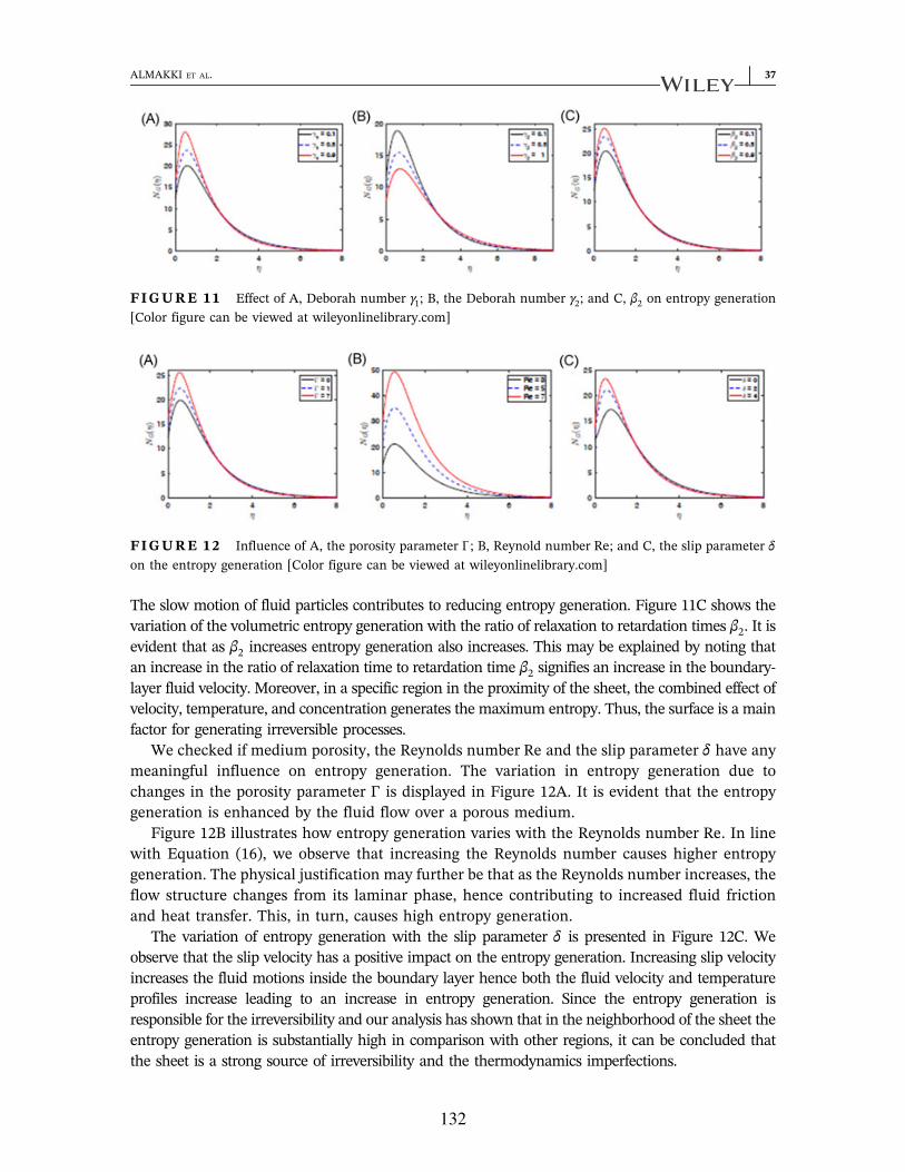
The slow motion of fluid particles contributes to reducing entropy generation. Figure 11C shows thevariation of the volumetric entropy generation with the ratio of relaxation to retardation times β2. It isevident that as β2 increases entropy generation also increases. This may be explained by noting thatan increase in the ratio of relaxation time to retardation time β2 signifies an increase in the boundary‐layer fluid velocity. Moreover, in a specific region in the proximity of the sheet, the combined effect ofvelocity, temperature, and concentration generates the maximum entropy. Thus, the surface is a mainfactor for generating irreversible processes.

We checked if medium porosity, the Reynolds number Re and the slip parameter δ have anymeaningful influence on entropy generation. The variation in entropy generation due tochanges in the porosity parameter Γ is displayed in Figure 12A. It is evident that the entropygeneration is enhanced by the fluid flow over a porous medium.

Figure 12B illustrates how entropy generation varies with the Reynolds number Re. In linewith Equation (16), we observe that increasing the Reynolds number causes higher entropygeneration. The physical justification may further be that as the Reynolds number increases, theflow structure changes from its laminar phase, hence contributing to increased fluid frictionand heat transfer. This, in turn, causes high entropy generation.

The variation of entropy generation with the slip parameter δ is presented in Figure 12C. Weobserve that the slip velocity has a positive impact on the entropy generation. Increasing slip velocityincreases the fluid motions inside the boundary layer hence both the fluid velocity and temperatureprofiles increase leading to an increase in entropy generation. Since the entropy generation isresponsible for the irreversibility and our analysis has shown that in the neighborhood of the sheet theentropy generation is substantially high in comparison with other regions, it can be concluded thatthe sheet is a strong source of irreversibility and the thermodynamics imperfections.

FIGURE 11 Effect of A, Deborah number γ1; B, the Deborah number γ2; and C, β2 on entropy generation[Color figure can be viewed at wileyonlinelibrary.com]

FIGURE 12 Influence of A, the porosity parameter Γ; B, Reynold number Re; and C, the slip parameter δon the entropy generation [Color figure can be viewed at wileyonlinelibrary.com]

ALMAKKI ET AL. | 37

132

In Section 2, it was shown that there are some sources of irreversibility, namely, thermalradiation, the magnetic field and mean absorption coefficient, viscous dissipation and fluidfriction and concentration diffusion. In Figure 13, the contribution of each source to the totalirreversibility is given as a function of distance from the sheet. First, it is observed, though notvery noticeable, that in the proximity of the sheet all sources of irreversibility contributepositively to the total irreversibility. However, the irreversibility due to the concentrationdiffusion (γdif ) is dominant due to the high Brownian motion of the nanoparticle species nearthe sheet. Moving away from the sheet the irreversibility due to the magnetic field and meanabsorption coefficient (γm) takes over and becomes the dominant source of irreversibility as thetemperature drops. On the other hand, the contribution of irreversibility due to concentrationdiffusion decreases moving away from the sheet due to a decrease in the Brownian motion. Thecombined effect of the increase in the magnetic field and the decrease in nanoparticle motionleads to the dominance of the irreversibility in the regions far from the sheet.

6 | CONCLUSION

We have presented a single generalized model for the study of steady two‐dimensional MHD flow andheat transfer in Jeffrey, Maxwell, and Oldroyd‐B nanofluids. Entropy generation, and how this isinfluenced by certain physical parameters has been investigated. The Deborah number has asignificant impact on entropy generation in porous media systems. Consequently, by varying theDeborah the entropy generation can be adjusted and controlled. A comparison of the accuracy ofthree spectral collocation techniques for solving highly nonlinear equations has been given. Thespectral relaxation method has been shown to give less residual errors, and this method has been usedto find the numerical solutions presented in this study. The main results of the analysis are, that

1. The velocity profiles increase with the Deborah number γ1, whereas the opposite trend wasobserved for temperature and concentration profiles.

2. The slip parameter has a negative impact on the velocity, temperature, and concentration profiles.3. Entropy generation increased with the Deborah number related to relaxation time γ1 and

decreased with the Deborah number related to retardation time γ2.4. The velocity, temperature, and concentration profiles are determined and subsequently used

to calculate the entropy generation number.5. The surface is hugely responsible for the irreversibility.

FIGURE 13 The impact of each source of irreversibility [Color figure can be viewed at wileyonlinelibrary.com]

38 | ALMAKKI ET AL.

133

6. The entropy generation due to concentration diffusion is the most dominant source ofentropy generation.

There are emerging research directions, which extend the classical studies by consider theentropy generation in natural and mixed convection.

ACKNOWLEDGMENTS

The authors would like to thank the University of KwaZulu‐Natal, South Africa, the DST‐NRFCentre of Excellence‐Mathematical and Statistical Sciences, and Amity University, Kolkata,India for financial support.

ORCID

Sabyasachi Mondal http://orcid.org/0000-0003-4666-0568

NOMENCLATURE

u velocity in x direction (m s−1)v velocity in y direction (m s−1)x, y( ) coordinate axis (m)

β1 fluid relaxation time (s)p pressureρf densityυf kinematic viscosity (m2 s−1)μ viscosity of the fluid (kg m−1 s−1)β2 ratio between relaxation time and retardation timeβ3 fluid retardation time (s)σ electrical conductivity (Ω−1 m−1)B0 magnetic field strength (kg s−2 A−1)K permeability coefficient (kgmN−1 s−1)T temperature (K)∞T ambient temperature (K)Tω temperature of the fluid at the sheet (K)κf thermal conductivity (Wm−1 K−1)cp specific heat (m2 s−2 K−1)τ effective heat capacity of nanoparticles (J K)pc( )p p heat capacity of the nanoparticles (J kg−1 K−1)

DB Brownian motion coefficient (kg m−1 s−1)C concentration of fluid (kgm−3)Cω concentration at the wall (kgm−3)∞C concentration away from the disk (kgm−3)DT thermophoretic diffusion coefficient (kg m−1 s−1 K−1)σ ⁎ Stefan‐Boltzmann constantκ⁎ Roseland mean absorption coefficient (m2 kg−1)u x( )ω velocity of the stretching sheet (m s−1)u x( )slip slip velocity (m s−1)hf heat transfer coefficient (Wm−2 K−1)

ALMAKKI ET AL. | 39

134

a, c( ) constants∞U x( ) velocity of free stream (m s−1)f dimensionless velocityη dimensionless variableθ dimensionless temperatureϕ dimensionless nanoparticle concentrationγ1 Deborah number due to retardation timeγ2 Deborah number due to relaxation timeα constantM magnetic field parameterΓ porosity parameterNr thermal radiation parameterPr Prandtl numberNt thermophoresis parameterEc Eckert numberNb Brownian motion parameterSc Schmidt numbers suction/injection parameterδ dimensionless velocity slip parameterBi Biot numberS′gen

′′ volumetric entropy generation (Wm−3 K−1)S ′0 ′′ dimensionless minimum entropy generation rateRe Reynold numberBr Brinkman numberΩ dimensionless

TΔ difference between ∞−T T( )(K)ωχ concentration difference

REFERENCES

1. Sandeep N, Rushi kumar B, Jagadeesh kumar MS. A comparative study of convective heat and mass transferin non‐newtonian nanofluid flow past a permeable stretching sheet. J Mol Liq. 2015;212:585‐591.

2. Sandeep N, Sulochana C. Momentum and heat transfer behaviour of jeffrey, maxwell and oldroyd‐bnanofluids past a stretching surface with non‐uniform heat source/sink. Ain Shams Eng J. 2016. https://doi.org/10.1016/j.asej.2016.02.008

3. Hayat T, Abbas Z, Sajid M. Series solution for the upper‐convected maxwell fluid over a porous stretchingplate. Phys Lett A. 2006;358(5–6):396‐403.

4. Abbasi F, Shehzad S, Hayat T, Alsaedi A, Obid MA. Influence of heat and mass flux conditions inhydromagnetic flow of jeffrey nanofluid. AIP Adv. 2015;5(3):037111.

5. Hussain T, Shehzad SA, Hayat T, Alsaedi A, Al‐Solamy F, Ramzan M. Radiative hydromag‐netic flow ofjeffrey nanofluid by an exponentially stretching sheet. PLOS One. 2014;9(8):e103719.

6. Rashidi MM, Freidoonimehr N, Hosseini A, Bég OA, Hung T‐K. Homotopy simulation of nanofluid dynamicsfrom a non‐linearly stretching isothermal permeable sheet with transpiration. Meccanica. 2014;49(2):469‐482.

7. Ramzan M, Bilal M, Chung JD, Mann A. On mhd rditive jeffery nnofluid flow with convective heat and massboundry conditions. Neural Comput Appl. 2017:1‐10. https://doi.org/10.1007/s00521-017-2852-8

8. Sheikholeslami M, Rashidi MM, Ganji DD. Effect of non‐uniform magnetic field on forced convection heattransfer of fe3o4–water nanofluid. Comput Methods Appl Mech Eng. 2015;294:299‐312.

9. Mustafa M, Hayat T, Hendi AA. Influence of melting heat transfer in the stagnation‐point flow of a jeffreyfluid in the presence of viscous dissipation. J Appl Mech. 2012;79(2):024501.

40 | ALMAKKI ET AL.

135

10. Mushtaq A, Mustafa M, Hayat T, Alsaedi A. Effects of thermal radiation on the stagnation‐point flow ofupper‐convected maxwell fluid over a stretching sheet. J Aerosp Eng. 2013;27(no. 4):04014015.

11. Satya narayana PV, Harish babu D. Numerical study of mhd heat and mass transfer of a jeffrey fluid over astretching sheet with chemical reaction and thermal radiation. J Taiwan Inst Chem Eng. 2016;59:18‐25.

12. Mustafa M, Khan JA, Hayat T, Alsaedi A. Simulations for maxwell fluid flow past a convectively heatedexponentially stretching sheet with nanoparticles. AIP Adv. 2015;5(3):037133.

13. Pires M, Sequeira A. Flows of generalized oldroyd‐b fluids in curved pipes. Parabolic Problems. Springer; 2011:21‐43.14. Nadeem S, Ul haq R, Akbar NS, Lee C, Khan ZH. Numerical study of boundary layer flow and heat transfer

of oldroyd‐b nanofluid towards a stretching sheet. PLOS One. 2013;8(8):e69811.15. Shehzad SA, Abdullah Z, Abbasi FM, Hayat T, Alsaedi A. Magnetic field effect in three‐dimensional flow of

an oldroyd‐b nanofluid over a radiative surface. J Magn Magn Mater. 2016;399:97‐108.16. Hayat T, Muhammad T, Shehzad SA, Alsaedi A. An analytical solution for magnetohydrodynamic oldroyd‐b

nanofluid flow induced by a stretching sheet with heat generation/absorption. Int J Therm Sci. 2017;111:274‐288.17. Abbas M, Bai Y, Rashidi M, Bhatti M. Analysis of entropy generation in the flow of peristaltic nanofluids in

channels with compliant walls. Entropy. 2016;18(3):90.18. Rashidi M, Mohammadi F, Abbasbandy S, Alhuthali M. Entropy generation analysis for stagnation point

flow in a porous medium over a permeable stretching surface. J Appl Fluid Mech. 2015;8(4):753‐765.19. Bejan A. Entropy generation minimization: The new thermodynamics of finite‐size devices and finite‐time

processes. J Appl Phys. 1996;79(3):1191‐1218.20. Oztop HF, Al‐Salem K. A review on entropy generation in natural and mixed convection heat transfer for

energy systems. Renewable Sustainable Energy Rev. 2012;16(1):911‐920.21. Dalir N. Numerical study of entropy generation for forced convection flow and heat transfer of a Jeffrey fluid

over a stretching sheet. Alexandria Eng J. 2014;53(4):769‐778.22. Rehman S, Haq R, Khan ZH, Lee C. Entropy generation analysis for non‐newtonian nanofluid with zero

normal flux of nanoparticles at the stretching surface. J Taiwan Inst Chem Eng. 2016;63:226‐235.23. Dalir N, Dehsara M, Nourazar SS. Entropy analysis for magnetohydrodynamic flow and heat transfer of a

jeffrey nanofluid over a stretching sheet. Energy. 2015;79:351‐362.24. Shateyi S, Motsa S, Makukula Z. On spectral relaxation method for entropy generation on a mhd flow and

heat transfer of a maxwell fluid. J Appl Fluid Mech. 2015;8(1):21‐31.25. Rashidi MM, Abelman S, Freidooni mehr N. Entropy generation in steady mhd flow due to a rotating porous

disk in a nanofluid. Int J Heat Mass Transfer. 2013;62:515‐525.26. Motsa SS, Dlamini PG, Khumalo M. Spectral relaxation method and spectral quasilinearization method for

solving unsteady boundary layer flow problems. Adv Math Phys. 2014;2014:1‐12.27. Motsa SS. A new spectral local linearization method for nonlinear boundary layer flow problems. J Appl

Math. 2013;2013:1‐15.28. Woods LC. The Thermodynamics of Fluid Systems. Oxford University Press, New York: Oxford, Clarendon

Press; 1975; 371p. http://adsabs.harvard.edu/abs/1975cp...book.....W29. Yamaguchi H. Engineering fluid mechanics. 85. Springer Science & Business Media; 2008. https://doi.org/10.

1007/978-1-4020-6742-630. Bejan A. Entropy generation minimization. Adv Eng Thermodyn. 2016:531‐600. https://doi.org/10.1002/

9781119245964.ch1131. Awad FG, Ahamed SMS, Sibanda P, Khumalo M. The effect of thermophoresis on unsteady oldroyd‐b

nanofluid flow over stretching surface. PLOS One. 2015;10(8):e0135914.

How to cite this article: Almakki M, Nandy SK, Mondal S, Sibanda P, Sibanda D.A model for entropy generation in stagnation‐point flow of non‐Newtonian Jeffrey,Maxwell, and Oldroyd‐B nanofluids. Heat Transfer—Asian Res. 2019;48:24‐41.https://doi.org/10.1002/htj.21366

ALMAKKI ET AL. | 41

136

Chapter 7

Conclusion

In this thesis we sought to investigate entropy generation, and heat and mass transfer in Newtonian

and non-Newtonian fluids in various geometrical settings and subject to different boundary condi-

tions. The resultant systems of equations that model the fluid flows of interest are highly nonlinear,

coupled, differential equations. Recent, spectral schemes were proposed for use in solving such

complex systems of equations. The impact of key physical and chemical parameters of the fluid

flows were analysed.

In Chapter 2, we investigated entropy generation and the combined effect of Soret and Dufour num-

bers in axisymmetric unsteady MHD nanofluid flow over a nonlinearly stretching sheet. The heat

flux at the boundary layer was assumed to be controlled. The velocity of the surface stretch was

assumed to be nonlinear in the radial direction. The magnetic field and chemical reaction were

each considered to be functions of both space and time. Brownian motion and thermophoresis

were considered to be significant. The spectral quasilinearization method was chosen as the so-

lution method for the system. It was found that the Hartmann number is proportionally related to

the skin friction, whereas the Sherwood and the Nusselt number decrease as the Hartmann number

increases. The Brinkman and the Reynolds numbers both have a positive effect on entropy gener-

ation. The results obtained conform with those results from similar previous studies published in

the literature.

In Chapter 3 we investigated heat and mass transfer and entropy generation in an unsteady two-

dimensional MHD flow of a magneto-micropolar fluid with boundary layer flow along a linear

137

porous sheet. The viscous dissipation, thermophoesis, nanoparticle Brownian motion, chemical

reaction and thermal radiation were taken into account. The bivariate spectral quasilinearization

method was used to solve the partial differential equations. It was found that the method converges

rapidly and gives accurate results. An increase in the Brownian motion parameter increases the

temperature profiles whereas the same increase in the Brownian motion parameter reduces the

concentration profiles. The Nusselt number and skin-friction coefficient increase with increasing

thermal radiation. Perhaps, the most significant finding emerging from this Chapter is that the

irreversibility due to thermal diffusion is the most dominant source of entropy generation. Further,

the surface contributes significantly to the irreversibility.

In Chapter 4,we studied entropy generation and the impact of the Bejan number on an MHD vis-

coelastic nanofluid flow with partial slip and homogeneous and heterogeneous reactions. The non-

linear thermal radiation, thermophoresis and Brownian motion were considered to be significant

factors that may alter the flow structure and the heat transfer properties of the fluid. The partial dif-

ferential equations were solved using the spectral quasilinearization method. It was found that the

Bejan number is strongly affected by variations in the viscoelastic parameter and the dimension-

less Brinkman groups. The entropy generation decreases with an increase in the viscoelastic and

partial slip parameters, while the entropy generation increases when the Brinkman and Reynolds

numbers increase.

In Chapter 5, we generalized a mathematical model to describe the flow of a steady incompressible

MHD Casson nanofluid with a binary chemical reaction flowing over a stretching or shrinking

sheet. The model was used to investigate heat transfer and entropy generation in the laminar

boundary-layer stagnation point. The external magnetic field, nonlinear thermal radiation and

viscous dissipation were considered to be significant factors. The system of ordinary differential

equations was solved numerically using the spectral quasilinearization method. We observed that

the velocity and temperature profiles decrease as the Casson parameter increases. The entropy

generation increases in response to an increase in Reynolds number.

In Chapter 6, a mathematical model was formulated to describe the behaviour of Jeffrey, Maxwell

138

and Oldroyd-B nanofluids. The model was used to investigate heat and mass transfer and en-

tropy generation near a stagnation point. The flow was subject to the magnetic field, the Brownian

motion, the slip velocity and the thermophoresis. Three different solution techniques were used;

namely, the spectral relaxation method, the spectral quasilinearization method and the spectral lo-

cal linearization method. A comparison of the accuracy of the three spectral collocation methods

was carried out through calculation and analysis of residual errors. We showed that the spectral

relaxation method gives smaller residual errors. For this reason, the spectral relaxation method was

used to solve the system of equations. In terms of the chemical and physical parameters, the slip

parameter has a negative influence on the velocity, temperature and concentration profiles. The

velocity profiles are proportionally related to the Deborah number whereas the opposite trend is

observed for temperature and concentration profiles. Entropy generation decreases with the Debo-

rah number related to retardation time whereas the opposite behaviour is noted with the Deborah

number related to relaxation time. The entropy generation due to concentration diffusion is the

most dominant source of entropy generation.

For future work, the credibility of the findings of this study, which are obtained merely through

mathematical modelling techniques, may be subjected to experiments for validation. The com-

plexity of the full model equations necessitates improving solution methods to obtain higher con-

vergence rates, greater stability and accuracy and improved portability of algorithms.

139

References

[1] M. Goyal and R. Bhargava, “Boundary layer flow and heat transfer of Viscoelastic nanoflu-

ids past a stretching sheet with partial slip conditions,” Applied Nanoscience, vol. 4, no. 6,

pp. 761–767, 2014.

[2] N. Dalir, “Numerical study of entropy generation for forced convection flow and heat transfer

of a Jeffrey fluid over a stretching sheet,” Alexandria Engineering Journal, vol. 53, no. 4,

pp. 769–778, 2014.

[3] N. Freidoonimehr and A. B. Rahimi, “Exact-solution of entropy generation for MHD

nanofluid flow induced by a stretching/shrinking sheet with transpiration: Dual solution,”

Advanced Powder Technology, vol. 28, no. 2, pp. 671–685, 2017.

[4] A. Bejan, “Entropy generation minimization: The new thermodynamics of finite-size devices

and finite-time processes,” Journal of Applied Physics, vol. 79, no. 3, pp. 1191–1218, 1996.

[5] M. I. Afridi, M. Qasim, I. Khan, S. Shafie, and A. S. Alshomrani, “Entropy generation in

magnetohydrodynamic mixed convection flow over an inclined stretching sheet,” Entropy,

vol. 19, no. 1, p. 10, 2016.

[6] R. Ellahi, S. Z. Alamri, A. Basit, and A. Majeed, “Effects of MHD and slip on heat transfer

boundary layer flow over a moving plate based on specific entropy generation,” Journal of

Taibah University for Science, pp. 1–7, 2018.

[7] M. H. Yazdi, S. Abdullah, I. Hashim, and K. Sopian, “Entropy generation analysis of open

parallel Microchannels embedded within a permeable continuous moving surface: applica-

tion to magnetohydrodynamics (MHD),” Entropy, vol. 14, no. 1, pp. 1–23, 2011.

[8] M. H. Matin, “Entropy analysis of combined heat and mass transfer over a plate embedded

140

in a porous medium,” Journal of Mechanical Engineering and Automation, vol. 5, no. 3A,

pp. 26–32, 2015.

[9] A. S. Butta, S. Munawara, A. Ali, and A. Mehmood, “Entropy analysis of mixed convective

magnetohydrodynamic flow of a Viscoelastic fluid over a stretching sheet,” Zeitschrift für

Naturforschung A, vol. 67, no. 8-9, pp. 451–459, 2012.

[10] M. H. Abolbashari, N. Freidoonimehr, F. Nazari, and M. M. Rashidi, “Analytical modeling

of entropy generation for Casson nanofluid flow induced by a stretching surface,” Advanced

Powder Technology, vol. 26, no. 2, pp. 542–552, 2015.

[11] J. Qing, M. M. Bhatti, M. A. Abbas, M. M. Rashidi, and M. E.-S. Ali, “Entropy generation

on MHD Casson nanofluid flow over a porous stretching/shrinking surface,” Entropy, vol. 18,

no. 4, p. 123, 2016.

[12] Y. A. Cengel and A. Ghajar, Heat and mass transfer (a practical approach, SI version).

McGraw-Hill Education„ McGraw-Hill Education, New York, 2011.

[13] C. A. Yunus and J. G. Afshin, Heat and mass transfer: fundamentals and applications. Tata

McGraw-Hill, New Delhi, 2011.

[14] T. L. Bergman, F. P. Incropera, D. P. DeWitt, and A. S. Lavine, Fundamentals of heat and

mass transfer. John Wiley & Sons, Hoboken, 2011.

[15] J. Buongiorno, “Convective transport in nanofluids,” Journal of Heat Transfer, vol. 128, no. 3,

pp. 240–250, 2006.

[16] S. Chol and J. Estman, “Enhancing thermal conductivity of fluids with nanoparticles,” ASME-

Publications-Fed, vol. 231, pp. 99–106, 1995.

[17] W. Yu and H. Xie, “A review on nanofluids: preparation, stability mechanisms, and applica-

tions,” Journal of Nanomaterials, vol. 2012, p. 1, 2012.

141

[18] A. Ghadimi, R. Saidur, and H. Metselaar, “A review of nanofluid stability properties and

characterization in stationary conditions,” International Journal of Heat and Mass Transfer,

vol. 54, no. 17-18, pp. 4051–4068, 2011.

[19] A. Kuznetsov and D. Nield, “Natural convective boundary-layer flow of a nanofluid past a

vertical plate,” International Journal of Thermal Sciences, vol. 49, no. 2, pp. 243–247, 2010.

[20] A. M. Rohni, S. Ahmad, and I. Pop, “Flow and heat transfer over an unsteady shrinking

sheet with suction in nanofluids,” International Journal of Heat and Mass Transfer, vol. 55,

no. 7-8, pp. 1888–1895, 2012.

[21] B. Gireesha and N. Rudraswamy, “Chemical reaction on MHD flow and heat transfer of a

nanofluid near the stagnation point over a permeable stretching surface with non-uniform heat

source/sink,” International Journal of Engineering, Science and Technology, vol. 6, no. 5,

pp. 13–25, 2014.

[22] O. D. Makinde and A. Aziz, “Boundary layer flow of a nanofluid past a stretching sheet with

a convective boundary condition,” International Journal of Thermal Sciences, vol. 50, no. 7,

pp. 1326–1332, 2011.

[23] N. S. Akbar, S. Nadeem, R. U. Haq, and Z. Khan, “Radiation effects on MHD stagnation

point flow of nanofluid towards a stretching surface with convective boundary condition,”

Chinese Journal of Aeronautics, vol. 26, no. 6, pp. 1389–1397, 2013.

[24] M. Rahman and I. Eltayeb, “Radiative heat transfer in a hydromagnetic nanofluid past a

nonlinear stretching surface with convective boundary condition,” Meccanica, vol. 48, no. 3,

pp. 601–615, 2013.

[25] S. Nadeem and R. U. Haq, “Effect of thermal radiation for megnetohydrodynamic bound-

ary layer flow of a nanofluid past a stretching sheet with convective boundary conditions,”

Journal of Computational and Theoretical Nanoscience, vol. 11, no. 1, pp. 32–40, 2014.

142

[26] N. Sandeep, B. R. Kumar, and M. J. Kumar, “A comparative study of convective heat and

mass transfer in non-Newtonian nanofluid flow past a permeable stretching sheet,” Journal of

Molecular Liquids, vol. 212, pp. 585–591, 2015.

[27] T. Hayat, Z. Abbas, and M. Sajid, “Series solution for the upper-convected Maxwell fluid

over a porous stretching plate,” Physics Letters A, vol. 358, no. 5-6, pp. 396–403, 2006.

[28] M. Ramzan, M. Bilal, J. D. Chung, and A. Mann, “On MHD radiative Jeffery nanofluid flow

with convective heat and mass boundary conditions,” Neural Computing and Applications,

pp. 1–10, 2017.

[29] A. Noghrehabadi, R. Pourrajab, and M. Ghalambaz, “Flow and heat transfer of nanofluids

over stretching sheet taking into account partial slip and thermal convective boundary condi-

tions,” Heat and Mass Transfer, vol. 49, no. 9, pp. 1357–1366, 2013.

[30] W. Ibrahim and B. Shankar, “MHD boundary layer flow and heat transfer of a nanofluid past

a permeable stretching sheet with velocity, thermal and solutal slip boundary conditions,”

Computers & Fluids, vol. 75, pp. 1–10, 2013.

[31] A. Noghrehabadi and A. Behseresht, “Flow and heat transfer affected by variable proper-

ties of nanofluids in natural-convection over a vertical cone in porous media,” Computers &

Fluids, vol. 88, pp. 313–325, 2013.

[32] N. Amirsom, M. Uddin, and A. Ismail, “Three dimensional stagnation point flow of bio-

nanofluid with variable transport properties,” Alexandria Engineering Journal, vol. 55, no. 3,

pp. 1983–1993, 2016.

[33] P. Sanghera, Quantum Physics for Scientists and Technologists: Fundamental Principles and

Applications for Biologists, Chemists, Computer Scientists, and Nanotechnologists. John

Wiley & Sons, New Jersey, 2011.

[34] F. Abbasi, S. Shehzad, T. Hayat, A. Alsaedi, and M. A. Obid, “Influence of heat and mass

flux conditions in hydromagnetic flow of Jeffrey nanofluid,” AIP Advances, vol. 5, no. 3,

p. 037111, 2015.

143

[35] M. Sheikholeslami, D. D. Ganji, M. Y. Javed, and R. Ellahi, “Effect of thermal radiation

on magnetohydrodynamics nanofluid flow and heat transfer by means of two phase model,”

Journal of Magnetism and Magnetic Materials, vol. 374, pp. 36–43, 2015.

[36] D. Pal, “Heat and mass transfer in stagnation-point flow towards a stretching surface in the

presence of buoyancy force and thermal radiation,” Meccanica, vol. 44, no. 2, pp. 145–158,

2009.

[37] H. F. Oztop and K. Al-Salem, “A review on entropy generation in natural and mixed convec-

tion heat transfer for energy systems,” Renewable and Sustainable Energy Reviews, vol. 16,

no. 1, pp. 911–920, 2012.

[38] M. M. Rashidi, M. M. Bhatti, M. A. Abbas, and M. E.-S. Ali, “Entropy generation on MHD

blood flow of nanofluid due to peristaltic waves,” Entropy, vol. 18, no. 4, p. 117, 2016.

[39] M. M. Bhatti, T. Abbas, M. M. Rashidi, and M. E.-S. Ali, “Numerical simulation of entropy

generation with thermal radiation on MHD Carreau nanofluid towards a shrinking sheet,”

Entropy, vol. 18, no. 6, p. 200, 2016.

[40] M. Magherbi, H. Abbassi, N. Hidouri, and A. B. Brahim, “Second law analysis in convective

heat and mass transfer,” Entropy, vol. 8, no. 1, pp. 1–17, 2006.

[41] A. S. Butt and A. Ali, “Entropy effects in hydromagnetic free convection flow past a vertical

plate embedded in a porous medium in the presence of thermal radiation,” The European

Physical Journal Plus, vol. 128, no. 5, p. 51, 2013.

[42] S. Baag, S. Mishra, G. Dash, and M. Acharya, “Entropy generation analysis for Viscoelastic

MHD flow over a stretching sheet embedded in a porous medium,” Ain Shams Engineering

Journal, vol. 8, no. 4, pp. 623–632, 2017.

[43] M. Almakki, S. Dey, S. Mondal, and P. Sibanda, “On unsteady three-dimensional axisymmet-

ric MHD nanofluid flow with entropy generation and thermo-diffusion effects on a nonlinear

stretching sheet,” Entropy, vol. 19, no. 7, p. 168, 2017.

144

[44] E. B. Gil, Experimental Design and Verification of a Centralized Controller for Irrigation

Canals. Elsevier, London, 2018.

[45] S. Alharbi and I. Hassanien, “Unsteady mixed convection flow in the stagnation region of

a heated vertical plate embedded in a variable porosity medium with thermal dispersion ef-

fects,” in Developments in Heat Transfer, pp. 217–226, Edited by Dr. Marco Aurelio Dos

Santos Bernardes, InTech, Shanghai, 2011.

[46] P. Patil, S. Roy, and I. Pop, “Unsteady mixed convection flow over a vertical stretching sheet

in a parallel free stream with variable wall temperature,” International Journal of Heat and

Mass Transfer, vol. 53, no. 21-22, pp. 4741–4748, 2010.

[47] Y. Lok, N. Amin, and I. Pop, “Unsteady mixed convection flow of a micropolar fluid near the

stagnation point on a vertical surface,” International Journal of Thermal Sciences, vol. 45,

no. 12, pp. 1149–1157, 2006.

[48] A. J. Chamkha and S. Ahmed, “Similarity solution for unsteady MHD flow near a stag-

nation point of a three-dimensional porous body with heat and mass transfer, heat genera-

tion/absorption and chemical reaction,” Journal of Applied Fluid Mechanics, vol. 4, no. 2,

pp. 87–94, 2011.

[49] R. Seshadri, N. Sreeshylan, and G. Nath, “Unsteady mixed convection flow in the stagnation

region of a heated vertical plate due to impulsive motion,” International Journal of Heat and

Mass Transfer, vol. 45, no. 6, pp. 1345–1352, 2002.

[50] R. Ravindran, M. Ganapathirao, and I. Pop, “Effects of chemical reaction and heat gener-

ation/absorption on unsteady mixed convection MHD flow over a vertical cone with non-

uniform slot mass transfer,” International Journal of Heat and Mass Transfer, vol. 73,

pp. 743–751, 2014.

[51] S. Liao, “Notes on the Homotopy analysis method: some definitions and theorems,” Com-

munications in Nonlinear Science and Numerical Simulation, vol. 14, no. 4, pp. 983–997,

2009.

145

[52] G. Adomian, Solving frontier problems of physics: The decomposition method. Kluwer, MA,

Boston, 1994.

[53] G. Adomian and G. Adomian, “A global method for solution of complex systems,” Mathe-

matical Modelling, vol. 5, no. 4, pp. 251–263, 1984.

[54] S.-J. Liao, “On the analytic solution of magnetohydrodynamic flows of non-Newtonian fluids

over a stretching sheet,” Journal of Fluid Mechanics, vol. 488, pp. 189–212, 2003.

[55] M. Ayub, A. Rasheed, and T. Hayat, “Exact flow of a third grade fluid past a porous plate

using Homotopy analysis method,” International Journal of Engineering Science, vol. 41,

no. 18, pp. 2091–2103, 2003.

[56] A. A. Afify, “Similarity solution in MHD: effects of thermal diffusion and diffusion thermo

on free convective heat and mass transfer over a stretching surface considering suction or

injection,” Communications in Nonlinear Science and Numerical Simulation, vol. 14, no. 5,

pp. 2202–2214, 2009.

[57] R. Sharma, R. Bhargava, and P. Bhargava, “A numerical solution of unsteady MHD convec-

tion heat and mass transfer past a semi-infinite vertical porous moving plate using element

free Galerkin method,” Computational Materials Science, vol. 48, no. 3, pp. 537–543, 2010.

[58] J. Argyris and M. Haase, “An engineer’s guide to soliton phenomena: Application of the

Finite element method,” Computer Methods in Applied Mechanics and Engineering, vol. 61,

no. 1, pp. 71–122, 1987.

[59] T. Cebeci and P. Bradshaw, “Finite-difference solution of boundary-layer equations,” in Phys-

ical and Computational Aspects of Convective Heat Transfer, pp. 385–428, Springer, 1984.

[60] A. Asaithambi, “A second-order Finite-difference method for the Falkner–Skan equation,”

Applied Mathematics and Computation, vol. 156, no. 3, pp. 779–786, 2004.

[61] S. S. Motsa, “A new spectral local linearization method for nonlinear boundary layer flow

problems,” Journal of Applied Mathematics, vol. 2013, Article ID 423628, 2013.

146

[62] S. S. Motsa, P. G. Dlamini, and M. Khumalo, “Spectral relaxation method and spectral quasi-

linearization method for solving unsteady boundary layer flow problems,” Advances in Math-

ematical Physics, vol. 2014, Article ID 341964, 2014.

[63] S. Motsa, T. Hayat, and O. Aldossary, “MHD flow of upper-convected Maxwell fluid over

porous stretching sheet using successive Taylor series linearization method,” Applied Mathe-

matics and Mechanics, vol. 33, no. 8, pp. 975–990, 2012.

[64] S. Motsa, V. Magagula, and P. Sibanda, “A bivariate Chebyshev spectral collocation quasilin-

earization method for nonlinear evolution parabolic equations,” The Scientific World Journal,

vol. 2014, Article ID 581987, 2014.

[65] S. Motsa and S. Shateyi, “Successive linearisation analysis of unsteady heat and mass transfer

from a stretching surface embedded in a porous medium with suction/injection and thermal

radiation effects,” The Canadian Journal of Chemical Engineering, vol. 90, no. 5, pp. 1323–

1335, 2012.

[66] S. Shateyi and S. Motsa, “Variable viscosity on magnetohydrodynamic fluid flow and heat

transfer over an unsteady stretching surface with hall effect,” Boundary Value Problems,

vol. 2010, no. 1, p. 257568, 2010.

[67] S. Motsa, “A new spectral relaxation method for similarity variable nonlinear boundary layer

flow systems,” Chemical Engineering Communications, vol. 201, no. 2, pp. 241–256, 2014.

[68] S. S. Motsa and P. Sibanda, “A multistage linearisation approach to a four-dimensional hy-

perchaotic system with cubic nonlinearity,” Nonlinear Dynamics, vol. 70, no. 1, pp. 651–657,

2012.

[69] S. Motsa, P. Dlamini, and M. Khumalo, “A new multistage spectral relaxation method for

solving chaotic initial value systems,” Nonlinear Dynamics, vol. 72, no. 1-2, pp. 265–283,

2013.

[70] C. Canuto, M. Y. Hussaini, A. Quarteroni, A. Thomas Jr, et al., Spectral methods in fluid

dynamics. Springer Science & Business Media, Virginia, 2012.

147

[71] J. P. Boyd, Chebyshev and Fourier spectral methods. Courier Corporation, New York, 2001.

[72] L. N. Trefethen, Spectral methods in MATLAB, vol. 10. Siam, 2000.

[73] R. E. Bellman and R. E. Kalaba, Quasilinearization and nonlinear boundary-value problems.

Rand Corporation, New York, 1965.

[74] S. S. Motsa and S. Shateyi, “The effects of chemical reaction, hall, and ion-slip currents

on MHD Micropolar fluid flow with thermal diffusivity using a novel numerical technique,”

Journal of Applied Mathematics, vol. 2012, Article ID 689015, 2012.

[75] J. S. Hesthaven, S. Gottlieb, and D. Gottlieb, Spectral methods for time-dependent problems,

vol. 21. Cambridge University Press, Rhode Island, 2007.

[76] S. S. Motsa and M. S. Ansari, “Unsteady boundary layer flow and heat transfer of Oldroyd-B

nanofluid towards a stretching sheet with variable thermal conductivity,” Thermal Science,

vol. 19, no. suppl. 1, pp. 239–248, 2015.

[77] G. Makanda, S. Shaw, and P. Sibanda, “Effects of radiation on MHD free convection of a

Casson fluid from a horizontal circular cylinder with partial slip in non-Darcy porous medium

with viscous dissipation,” Boundary Value Problems, vol. 2015, no. 1, p. 75, 2015.

148