A Numerical Modeling of Rayleigh-Marangoni Steady Convection in a Non-Uniform Differentially Heated...
22
115 0885-7474/04/0200-0115/0 © 2003 Plenum Publishing Corporation Journal of Scientific Computing, Vol. 20, No. 1, February 2004 (© 2003) A Numerical Modeling of Rayleigh–Marangoni Steady Convection in a Non-Uniform Differentially Heated 3D Cavity E. Bucchignani 1 and D. Mansutti 2 1 Centro Italiano Ricerche Aerospaziali, Via Maiorise, 81043 Capua (CE), Italy. E-mail: [email protected] 2 Istituto per le Applicazioni del Calcolo/C.N.R., Viale del Policlinico, 137, 00161 Roma, Italy. E-mail: [email protected] Received September 10, 2002; accepted (in revised form) October 28, 2002 A numerical study of a buoyancy driven convection flow in presence of ther- mocapillarity has been developed. The fluid is a silicone oil (Prandtl number equal to 105) contained in a three-dimensional box bounded by rigid and impermeable walls with top free surface exposed to a gaseous phase. At the lateral box walls a different non-uniform temperature distribution is assumed so to induce horizontal convection and to keep separated thermocapillary and buoyancy effects. The vorticity-velocity formulation of the time-dependent Navier–Stokes equations for a non-isothermal incompressible fluid is used. A procedure based on a linearized fully implicit finite difference second order scheme has been adopted. We obtained very complex steady configurations for several values of the temperature difference at the lateral walls, DT=30, 40 and 50°C. Along the direction perpendicular to the lateral walls, for DT increasing, we observe a physically meaningful growth of heat transfer. Confidence in these results is supported by a comparison with recent experimental and numerical observations. KEY WORDS: Free surface; Buoyancy; Thermocapillary; Convection. 1. INTRODUCTION Buoyancy and thermocapillary driven natural convection has relevance in a wide range of engineering and industrial applications with moving fronts such as crystal growth, glass manufacturing, welding material processing,
Transcript of A Numerical Modeling of Rayleigh-Marangoni Steady Convection in a Non-Uniform Differentially Heated...

115
0885-7474/04/0200-0115/0 © 2003 Plenum Publishing Corporation
Journal of Scientific Computing, Vol. 20, No. 1, February 2004 (© 2003)
A Numerical Modeling of Rayleigh–Marangoni SteadyConvection in a Non-Uniform Differentially Heated 3DCavity
E. Bucchignani1 and D. Mansutti2
1 Centro Italiano Ricerche Aerospaziali, Via Maiorise, 81043 Capua (CE), Italy. E-mail:[email protected] Istituto per le Applicazioni del Calcolo/C.N.R., Viale del Policlinico, 137, 00161 Roma,
Italy. E-mail: [email protected]
Received September 10, 2002; accepted (in revised form) October 28, 2002
A numerical study of a buoyancy driven convection flow in presence of ther-mocapillarity has been developed. The fluid is a silicone oil (Prandtl numberequal to 105) contained in a three-dimensional box bounded by rigid andimpermeable walls with top free surface exposed to a gaseous phase. At thelateral box walls a different non-uniform temperature distribution is assumed soto induce horizontal convection and to keep separated thermocapillary andbuoyancy effects. The vorticity-velocity formulation of the time-dependentNavier–Stokes equations for a non-isothermal incompressible fluid is used. Aprocedure based on a linearized fully implicit finite difference second orderscheme has been adopted. We obtained very complex steady configurations forseveral values of the temperature difference at the lateral walls, DT=30, 40 and50°C. Along the direction perpendicular to the lateral walls, for DT increasing,we observe a physically meaningful growth of heat transfer. Confidence in theseresults is supported by a comparison with recent experimental and numericalobservations.
KEY WORDS: Free surface; Buoyancy; Thermocapillary; Convection.
1. INTRODUCTION
Buoyancy and thermocapillary driven natural convection has relevance in awide range of engineering and industrial applications with moving frontssuch as crystal growth, glass manufacturing, welding material processing,
etc. In several applications a liquid material is enclosed in a three-dimen-sional box bounded by rigid and impermeable walls with top free surfaceand a horizontal temperature difference imposed at the vertical walls. Inthese conditions, horizontal convection sets in whereas the variability ofsurface tension with temperature leads to thermocapillary convection.While in large systems buoyancy forces are the dominant driving mecha-nism, in small scale systems or in low gravity environments surface tensionforces at the liquid/air interface play a significant role in determining thedynamics of the flow. Moreover Schwabe and Metzger [1] performed anexperimental work in order to investigate the importance of surface tensionforces to buoyant forces in crystal growth melts. They found that atmoderate values of the Prandtl number (Pr) (a measure of the fluid apti-tude towards momentum diffusion versus heat diffusion), around the valuePr=17, surface tension forces are always significant and the highest flowspeeds are always measured near the free surface.
The numerical studies of three-dimensional horizontal convectionflows published so far in the literature are just a few, some of them inclosed cavity [2], [3], and other ones in open top cavity [4], [5], [6].Janssen et al. in Ref. 2 described the first bifurcation step, from steady toperiodic flow, versus growing Rayleigh number (Ra)—increasing buoyancyforce—and discussed the instability mechanism responsible of such a tran-sition in both cases of water (Pr=7.) and air (Pr=0.71). Bucchignaniet al. in Ref. 3 reported the bifurcation pattern versus Ra for the one-cellflow of a liquid metal (Pr=0.015) in a closed shallow cavity starting fromsteady regime up to transition to chaos. In Ref. 4 Behnia et al. provided adetailed description of the steady flows in the case of a low Prandtl fluid(Pr=0.01) in an open top cubic cavity either with thermocapillary effectscounteracting the buoyancy force and with concurrent effects. Mundraneet al. studied in Ref. 5 the departure of a three-dimensional flow from atwo-dimensional configuration at Pr=8.4 as the Marangoni number (Ma)grows at constant Bond number (Bo=Ra/Ma)—that is with increasingthermocapillary force at fixed ratio of buoyancy to thermocapillary forces(Bo=5.76). Giangi et al. in Ref. 6 obtained the steady flow configurationsof a liquid metal (Pr=0.015) in a shallow cavity and observed the increaseof the three-dimensional effects and of the flow speed at the free top as Raincreases. The sparsity and fragmentation of these cited results is mainlydue to the high computational cost of the numerical tests characterized byquite lengthy transient regimes.
In the present numerical study, following Schwabe and Metzger [1],we have considered the motion of a viscous incompressible fluid in aparallelepipedic box bounded by rigid and impermeable walls with a topfree surface exposed to a gaseous phase. We impose a non-uniform
116 Bucchignani and Mansutti
temperature distribution at the lateral box of the wall so to inducehorizontal convection and to keep separated thermocapillary and buoyancyeffects. A very complex behavior of the flow and thermal fields springsfrom the interaction of the induced flow structures. The liquid considered isa silicone oil, a fluid very often used in space laboratory experiments; itsPrandtl number is Pr=105.
We solved the vorticity-velocity formulation of the time-dependentNavier–Stokes equations for a non-isothermal incompressible fluid. Aprocedure based on a linearized fully implicit finite difference second orderscheme has been adopted; the Bi-CGSTAB algorithm with a ILU precon-ditioner has been used to solve the linear systems. We computed steadyflow configurations with several values of the temperature difference at thelateral walls, DT=30, 40 and 50°C and at fixed Bo, that is at fixed ratio ofbuoyancy to thermocapillary forces. The numerical solutions are visualizedby means of LIC (Line Integral Convolution), which is a vector fieldrepresentation for the global realistic visualization of a surface flow [7].
This paper is organized as follows: in the next section we describe thephysical and geometrical domain, in Section 3 we provide the mathematicalformulation here adopted, in Section 4 we explain the numerical methodfor solution; the numerical results are discussed in Section 5 and finallyconclusions are drawn in Section 6.
2. DESCRIPTION OF THE FLOW DOMAIN
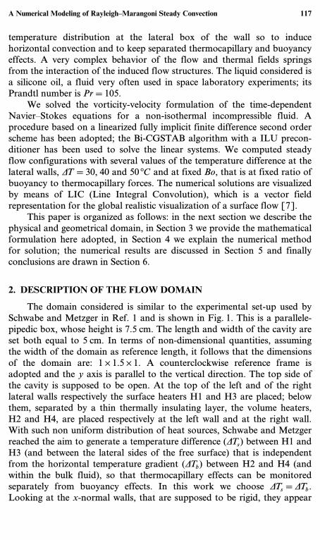
The domain considered is similar to the experimental set-up used bySchwabe and Metzger in Ref. 1 and is shown in Fig. 1. This is a parallele-pipedic box, whose height is 7.5 cm. The length and width of the cavity areset both equal to 5 cm. In terms of non-dimensional quantities, assumingthe width of the domain as reference length, it follows that the dimensionsof the domain are: 1×1.5×1. A counterclockwise reference frame isadopted and the y axis is parallel to the vertical direction. The top side ofthe cavity is supposed to be open. At the top of the left and of the rightlateral walls respectively the surface heaters H1 and H3 are placed; belowthem, separated by a thin thermally insulating layer, the volume heaters,H2 and H4, are placed respectively at the left wall and at the right wall.With such non uniform distribution of heat sources, Schwabe and Metzgerreached the aim to generate a temperature difference (DTs) between H1 andH3 (and between the lateral sides of the free surface) that is independentfrom the horizontal temperature gradient (DTb) between H2 and H4 (andwithin the bulk fluid), so that thermocapillary effects can be monitoredseparately from buoyancy effects. In this work we choose DTs=DTb.Looking at the x-normal walls, that are supposed to be rigid, they appear
A Numerical Modeling of Rayleigh–Marangoni Steady Convection 117

H4
H3
H2
H1
y
adiab.
z
x
T = 0.83
T = 0.33
free surface
adiab.
T = 0.83
T = 1.33
Fig. 1. Scheme of the computational domain.
ideally subdivided into three horizontal strips whose heights are, frombottom, 5, 2, and 0.5 cm. At the wall at x=0, the lower strip is isothermalat T=0.83 (non dimensional units), the middle one is adiabatic and theupper one is isothermal at T=0.33. At the wall at x=1, the lower strip isisothermal at T=1.33, the middle one is adiabatic and the upper one isisothermal at T=0.83. The z-normal walls and the bottom wall are rigidand adiabatic. At the open top, the free surface is supposed to be flat andadiabatic. We have re-normalized the temperature field by taking thehighest temperature difference among the boundary values, DT=1.33−0.33, as new temperature reference.
3. MATHEMATICAL FORMULATION
3.1. Governing Equations
An appropriate mathematical model for the motion of silicone oil inthis geometrical and physical setting is represented by the Navier–Stokesequations for an incompressible non-isothermal fluid with the Fourier–Boussinesq approximation. We adopt the formulation in terms of vorticity
118 Bucchignani and Mansutti

w, velocity u=(u, v, w) and temperature h in non-dimensional form. Thereference physical quantities are the following velocity ug and time tg
ug=c DT/m, tg=Lm/c DT
where we mean L the box width, DT the temperature difference defined inthe previous section, m the dynamic viscosity and c=−“s/“h the gradientof the surface tension with respect to temperature. Then the solved equa-tions appear:
MaPr“w
“t+MaPr
N×(w×u)=N2w−RaMa
N×1h g|g|2 (1)
N2u=−N×w (2)
“h
“t+(u ·N) h=
1Ma
N2h. (3)
where we remind that Pr is the Prandtl number of the fluid and Ra andMaare the non-dimensional parameters related to the flow, respectively theRayleigh number and the Marangoni number; they are defined as
Pr=n
oRa=
gbDTL3
onMa=
cDTLmo
and furthermore g is the magnitude of the gravitational acceleration, b isthe coefficient of thermal expansion, o is the thermal diffusivity and n is thekinematic viscosity.
The adopted non-dimensional scheme avoids the presence of non-dimensional parameters in the expressions of the boundary conditions onthe free surface. Moreover, due to the selected boundary values, thehorizontal temperature difference at the facing vertical walls and the ratioBo=Ma
Ra (Bond number) are constant.Although the above formulation is massively used for the simulation
of thermal convection applications, since a coherent reconstruction hasbeen finally provided by Rajagopal et al. in Ref. 8, we want to spend fewwords on its limitations, more precisely about the applicability of theBoussinesq approximation of the Navier–Stokes equations. It is knownthat this formulation describes a mechanically incompressible and ther-mally compressible fluid. Rajagopal et al. showed that it can be builtthrough a perturbation procedure applied to the equations for a linearlyviscous non-isothermal fluid in the non-dimensional form suggested byChandrasekhar [9]. For a certain perturbation parameter, it has beenshown that the Oberbeck–Boussinesq equations follow from keeping in the
A Numerical Modeling of Rayleigh–Marangoni Steady Convection 119

flow expansion terms up to the fourth order and selecting properly terms inthe full equations to be set to zero. In fact the resulting perturbative for-mulation appears inconsistent as the equations are not obtained, as theyshould be, by equating to zero the sums of the terms of the same order upto the fourth one. Nevertheless the Oberbeck–Boussinesq idea, as it allowsto cut off an equation from the differential system to be solved, is oftensuccessfully introduced in fluid dynamics when mass density variations canbe assumed linear versus temperature.
3.2. Boundary Conditions
Within the above formulation, boundary conditions assume a verysimple form:
• the boundary conditions associated to Eq. (1) are obtained by thevorticity definition written on the boundary. Due to the time discre-tization scheme used, this boundary condition is updated andenforced at each current time step. This procedure contributes to thecorrect coupling between the kinematic and the dynamic parts of theproblem;
• Dirichlet boundary conditions are associated to the elliptic velocityEq. (2). In particular null velocity field is assigned at the solid walls;at the top free surface, that is assumed to be flat, it holds:
v=0
“u“y=−
“h
“x
“w“y=−“h
“z
where the last two conditions are obtained by enforcing the seconddynamics law. We observe that the second condition above intro-duces a jump discontinuity at x=0 and x=1. Actually at thosecartesian planes the velocity component u is null due to the presenceof a rigid wall; consequently “u
“y is null. On the contrary, at the freesurface, “h
“x is a measure of the thermocapillary effects and is not at allvanishing. However this inconsistency of the formulation has noeffect within the numerical solution procedure here adopted becausethis is based on a finite difference discretization and the disconti-nuity edge is left out of the computational domain as if regularizedboundary values were imposed.
120 Bucchignani and Mansutti

• the boundary conditions for the energy equation are of Dirichlet orNeumann type in those portions of the boundary where respectivelythe value of temperature or its normal derivative are known (e.g. anadiabatic boundary yields to the assignment “h
“n=0).
4. SOLUTION PROCEDURE
The governing Eqs. (1), (2), (3) together with the proper boundaryconditions are discretized by using finite difference approximations. Spatialderivatives are discretized on a uniform mesh through central second-orderdifferences whilst time derivatives are discretized through three-pointsecond-order backward differences.
By the chosen finite difference schemes, the discrete model ensuresmaximum accuracy by a staggered variable location. At this purpose theMAC stencil, originally built for the (u, h) formulation by Harlow andWelch [10], has been adapted to the present (u, w, h) formulation. Ingeneral when each velocity component is evaluated at the middle of thefaces of the computational cell which are orthogonal, the mass conserva-tion law at the discrete level can be satisfied up to meet the round-off error.In a similar way, by evaluating the vorticity components at the mid-pointof the edges of the computational cell which are parallel, the natural prop-erty of solenoidality of the vorticity can be met at the discrete level up toround off error. Furthermore in our model staggering of the variablesallows to discretize the Eq. (2) without any need of variable averaging. Onthe contrary, in discretizing the Eq. (1), averaging is necessary for thetreatment of the advective term N×(w×u), where the product w×u is hereaveraged in the whole [11]. In this way the resulting discrete equation isconsistent with the implicit property of solenoidality of the vorticity fieldexpressed in discrete form.
The time-dependent analysis performed by the present method requireparticular care when used together with the vorticity-velocity formulation.In fact the continuity equation is imposed only in an implicit way bydropping the term N ·u in the Eqs. (1), (2), and (3) so that mass conserva-tion and definition of vorticity could be violated if good coupling amongthe full set of the equations is not ensured. Then the time integration hasbeen executed by means of a fully implicit numerical scheme that has beenafterwards linearized through the ‘‘frozen coefficients’’ technique [12].
In this way at each time step our original system of partial differentialequations gives rise to a large linear system of equations of the type
Ax=b
A Numerical Modeling of Rayleigh–Marangoni Steady Convection 121
where x is the unknown vector and b is the known vector. The coefficientmatrix A has a large sparse structure. The solution of this linear system viaa direct method is obviously not recommended due to the size of theproblem and an iterative procedure has been adopted, a variant of Pre-conditioned Conjugate Gradient. This approach has the advantage to allowa great flexibility in writing the discretized form of numerical model. Wehave used the Bi-CGSTAB algorithm [12, 13], because of its numericalstability and speed of convergence.
Although, from a theoretical point of view, iterative methods can beused without preconditioning the linear systems of equations, the use of apreconditioning technique is, in many practical applications, essential tofulfil the convergence and stability requirements of the iterative procedureitself. The aim of the preconditioner is to convert the original linear systemto an equivalent but better-conditioned system. This consists of finding areal matrix C such that the new linear system
C−1Ax=C−1b
has (by construction) better convergence and stability characteristics thanthe original system. It is obvious that the matrix C must be chosen care-fully so that C−1 should be close to the inverse of A and easy to be invertedin order to compress the computational cost. As a matter of fact the ILUfactorization is one of the most widely used preconditioners: C is defined asthe product LU of a lower (L) and an upper (U) triangular matrix gener-ated by a variant of the Crout factorization algorithm where only the ele-ments of A that are originally non-zero are factorized and stored. In thisway the sparsity structure of A is completely preserved.
The testing of the described numerical model has been extensively dis-cussed in Ref. 12. The numerical inaccuracies usually reported in meetingmass conservation and vorticity definition had the same order of magni-tude as the round-off error at each time step.
The numerical solutions have been visualized by means of LIC (LineIntegral Convolution), which is a vector field representation for the globalrealistic visualization of a surface flow [7]. In contrast to tracing singlestreamlines, the LIC technique is based on the tracing of a high number ofrelatively short streamlines, that are actually convoluted with an initiallyrandom distribution of black/white points on the target surface (seeds).Resulting LIC images appear very similar to some typical flow visualiza-tions (oil flow patterns), thus well suited for numerical-experimental com-parison. However, it is worth observing that LIC allows only qualitativecomparisons, therefore numerical tables are also included. The criterionused in order to assess the steadiness of the flow is based on the numerical
122 Bucchignani and Mansutti

evaluation of the time derivative of w averaged on the whole flow field:when this value is smaller than a fixed quantity (10−9) the flow is con-sidered steady.
5. NUMERICAL FLOWS
Here we solved the problem when the domain is filled with a siliconeoil characterized by the following thermophysical data: r=0.935 g cm−3,m=0.0935 g cm−1 s−1, c=0.068Dy cm−1 K−1, o=9.51 · 10−4 cm2 s−1; thePrandtl number results Pr=105. We treated the case DTb=DTs=DT. Thenumerical model described above was adopted to solve several thermalconvection flow problems in parallelepipedic domains and the computa-tional code was repeatedly validated as mentioned in Ref. 3. In the study ofthe horizontal thermal convection flow in a shallow three-dimensionalcavity, the space mesh sensitivity analysis leads the authors to the conclu-sion that a mesh with a spatial resolution of 0.05 is sufficient to obtainaccurate results [3]. Due to the physical similarities of the present flowproblem, we expect here that the same spatial resolution corresponding to a21 · 31 · 21 space grid might be sufficient to describe the whole flow struc-tures. It is worthwhile to mention that, by time and space mesh sensitivityanalysis developed in a two dimensional problem, it has been noted thatthis numerical model appears ‘‘nearly’’ second order accurate both in timeand in space as reported in Ref. 12. Actually the linearization procedureapplied to the convective terms within the discretized equations slightlylowers the degree of accuracy of the overall discrete operator with respectto the single discrete schemes used.
In such a setting we found by trial and error that the computationalprocedure requires a time step Dt less or equal to 10−2 as for larger valuesBi-CGSTAB iterations may not converge.
For the present physical problem a comparison with the numericalresults obtained by Savino et al. [14] was performed. A preliminary simu-lation was executed at temperature difference DT=15°C starting from restin order to compare with the experimental and numerical results obtainedby Savino et al. who developed the same test case by a control volumetechnique [14]. This value of DT provides Ra=2.1 · 107 andMa=5.7 · 104.We observe that after a finite time interval the convection flow reaches asteady configuration close to the one displayed by Savino et al.. Actually avery good agreement is reached versus the maximum value of the modulusof the velocity field, umax=0.2377 cm/sec, that is just 0.23% different fromthe value obtained by the other authors.
Further simulations have been developed assuming for the tempera-ture difference DT the values of 30°C, 40°C and 50°C. The values of Ra
A Numerical Modeling of Rayleigh–Marangoni Steady Convection 123
Table I. Rayleigh and Marangoni Numbers Consideredas a Function of DT
DT Ra Ma
Case 1 30°C 4.2 · 107 11.5 · 104
Case 2 40°C 5.6 · 107 15.3 · 104
Case 3 50°C 7.0 · 107 19.6 · 104
and Ma related to these temperature gradients are listed in Table I. It isassumed that initially the fluid is at rest at uniform temperature. In thethree cases considered the Bond number Bo has about the same value(Bo=2.73 · 10−3).
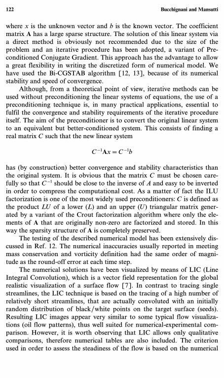
In each Case after a finite time interval, a steady regime is reached asit is shown in Fig. 2, where the transient history of the u velocity compo-nent at the point (0.4, 0.5, 0.4) is plotted for the Case 1 (DT=30°C). Inorder to definitely assess the validity of the chosen space resolution, we runthe Case 1 not only on the selected grid (21 · 31 · 21) but also on a finer one(31 · 41 · 31) and obtained a satisfactory agreement as it is reported by the
0
0.2
0.4
0.6
0.8
1
1.2
0 200 400 600 800 1000 1200
u (x
100
)
t
Fig. 2. Case 1, Ra=4.2 · 107 andMa=11.5 · 104—Time history of the u velocity componentat the point (0.4,0.5,0.4).
124 Bucchignani and Mansutti
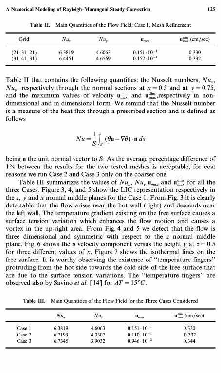
Table II. Main Quantities of the Flow Field; Case 1, Mesh Refinement
Grid Nux Nuy umax udimmax (cm/sec)
(21 · 31 · 21) 6.3819 4.6063 0.151 · 10−1 0.330(31 · 41 · 31) 6.4451 4.6569 0.152 · 10−1 0.332
Table II that contains the following quantities: the Nusselt numbers, Nux,Nuy, respectively through the normal sections at x=0.5 and at y=0.75,and the maximum values of velocity umax and udimmax,respectively in non-dimensional and in dimensional form. We remind that the Nusselt numberis a measure of the heat flux through a prescribed section and is defined asfollows
Nu=1SFS(hu−Nh) ·n ds
being n the unit normal vector to S. As the average percentage difference of1% between the results for the two tested meshes is acceptable, for costreasons we run Case 2 and Case 3 only on the coarser one.
Table III summarizes the values of Nux, Nuy,umax and udimmax for all thethree Cases. Figure 3, 4, and 5 show the LIC representation respectively inthe z, y and x normal middle planes for the Case 1. From Fig. 3 it is clearlydetectable that the flow arises near the hot wall (right) and descends nearthe left wall. The temperature gradient existing on the free surface causes asurface tension variation which enhances the flow motion and causes avortex in the up-right area. From Fig. 4 and 5 we detect that the flow isthree dimensional and symmetric with respect to the z normal middleplane. Fig. 6 shows the u velocity component versus the height y at z=0.5for three different values of x. Figure 7 shows the isothermal lines on thefree surface. It is worthy observing the existence of ‘‘temperature fingers’’protruding from the hot side towards the cold side of the free surface thatare due to the surface tension variations. The ‘‘temperature fingers’’ areobserved also by Savino et al. [14] for DT=15°C.
Table III. Main Quantities of the Flow Field for the Three Cases Considered
Nux Nuy umax udimmax (cm/sec)
Case 1 6.3819 4.6063 0.151 · 10−1 0.330Case 2 6.7199 4.0307 0.110 · 10−1 0.332Case 3 6.7345 3.9032 0.946 · 10−2 0.344
A Numerical Modeling of Rayleigh–Marangoni Steady Convection 125

Fig. 3. Case 1, Ra=4.2 · 107 and Ma=11.5 · 104—LIC representation at the z-normalmiddle section.
Fig. 4. Case 1, Ra=4.2 · 107 and Ma=11.5 · 104—LIC representation at the y-normalmiddle section.
126 Bucchignani and Mansutti
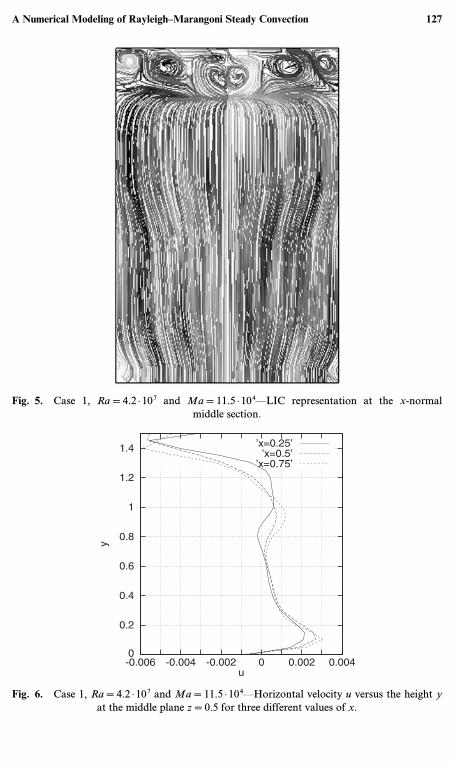
Fig. 5. Case 1, Ra=4.2 · 107 and Ma=11.5 · 104—LIC representation at the x-normalmiddle section.
0
0.2
0.4
0.6
0.8
1
1.2
1.4
-0.006 -0.004 -0.002 0 0.002 0.004
y
u
’x=0.25’’x=0.5’
’x=0.75’
Fig. 6. Case 1, Ra=4.2 · 107 and Ma=11.5 · 104—Horizontal velocity u versus the height yat the middle plane z=0.5 for three different values of x.
A Numerical Modeling of Rayleigh–Marangoni Steady Convection 127

0
0.2
0.4
0.6
0.8
1
0 0.2 0.4 0.6 0.8 1
Z
X
Fig. 7. Case 1, Ra=4.2 · 107 andMa=11.5 · 104 - Isothermal lines on the free surface.
Fig. 8. Case 2, Ra=5.6 · 107 and Ma=15.3 · 104—LIC representation at the z-normalmiddle section.
128 Bucchignani and Mansutti
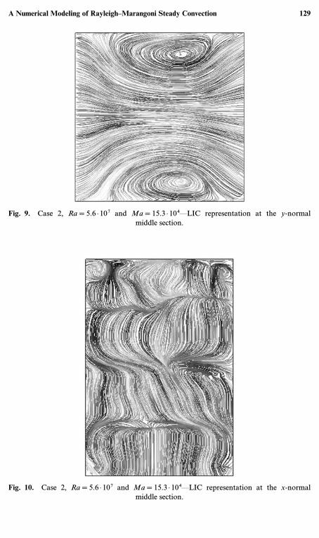
Fig. 9. Case 2, Ra=5.6 · 107 and Ma=15.3 · 104—LIC representation at the y-normalmiddle section.
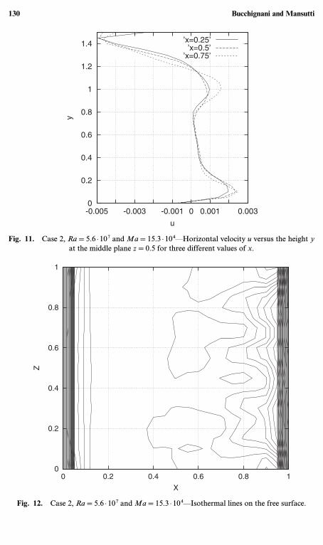
Fig. 10. Case 2, Ra=5.6 · 107 and Ma=15.3 · 104—LIC representation at the x-normalmiddle section.
A Numerical Modeling of Rayleigh–Marangoni Steady Convection 129
0
0.2
0.4
0.6
0.8
1
1.2
1.4
-0.005 -0.003 -0.001 0 0.001 0.003
y
u
’x=0.25’’x=0.5’
’x=0.75’
Fig. 11. Case 2, Ra=5.6 · 107 andMa=15.3 · 104—Horizontal velocity u versus the height yat the middle plane z=0.5 for three different values of x.
0
0.2
0.4
0.6
0.8
1
0 0.2 0.4 0.6 0.8 1
Z
X
Fig. 12. Case 2, Ra=5.6 · 107 andMa=15.3 · 104—Isothermal lines on the free surface.
130 Bucchignani and Mansutti

In Figures from 8 to 12 same plots are shown for the Case 2. The flowspeed increases and this fact induces several effects. The main vortex movesupwards and its strength augments (see Fig. 8); three-dimensional struc-tures become more evident (see Fig. 10) and symmetry with respect to the znormal middle plane is lost (see Fig. 9). The ‘‘temperature fingers’’ are lesspronounced (see Fig. 12). The increase of the temperature difference DTinduces also an increase of the surface tension gradient and the consequentapparition of a new vortex in the up-left area.
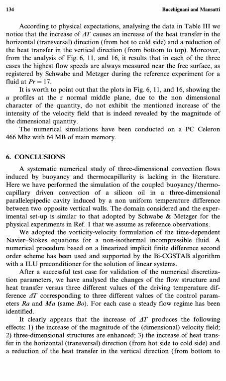
Figures from 13 to 17 provide an analogous description of the simula-tion of the Case 3. Here the general trend highlighted for the Case 2 isenhanced. The flow speed becomes larger and produces a fully developedthree-dimensional configuration. The ‘‘temperature fingers’’ are no morevisible (see Fig. 17).
Fig. 13. Case 3, Ra=7.0 · 107 and Ma=19.6 · 104—LIC representation at the z-normalmiddle section.
A Numerical Modeling of Rayleigh–Marangoni Steady Convection 131
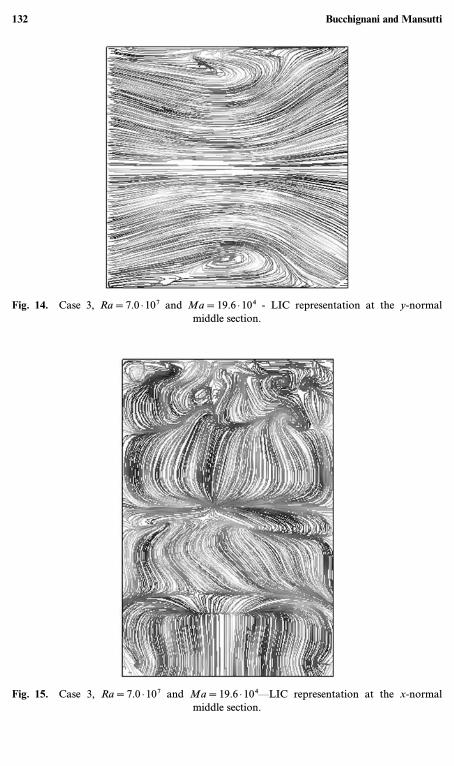
Fig. 14. Case 3, Ra=7.0 · 107 and Ma=19.6 · 104 - LIC representation at the y-normalmiddle section.
Fig. 15. Case 3, Ra=7.0 · 107 and Ma=19.6 · 104—LIC representation at the x-normalmiddle section.
132 Bucchignani and Mansutti

0
0.2
0.4
0.6
0.8
1
1.2
1.4
-0.005 -0.003 -0.001 0 0.001 0.003
y
u
’x=0.75’’x=0.5’
’x=0.25’
Fig. 16. Case 3, Ra=7.0 · 107 andMa=19.6 · 104—Horizontal velocity u versus the height yat the middle plane z=0.5 for three different values of x.
0
0.2
0.4
0.6
0.8
1
0 0.2 0.4 0.6 0.8 1
Z
X
Fig. 17. Case 3, Ra=7.0 · 107 andMa=19.6 · 104—Isothermal lines on the free surface.
A Numerical Modeling of Rayleigh–Marangoni Steady Convection 133
According to physical expectations, analysing the data in Table III wenotice that the increase of DT causes an increase of the heat transfer in thehorizontal (transversal) direction (from hot to cold side) and a reduction ofthe heat transfer in the vertical direction (from bottom to top). Moreover,from the analysis of Fig. 6, 11, and 16, it results that in each of the threecases the highest flow speeds are always measured near the free surface, asregistered by Schwabe and Metzger during the reference experiment for afluid at Pr=17.
It is worth to point out that the plots in Fig. 6, 11, and 16, showing theu profiles at the z normal middle plane, due to the non dimensionalcharacter of the quantity, do not exhibit the mentioned increase of theintensity of the velocity field that is indeed revealed by the magnitude ofthe dimensional quantity.
The numerical simulations have been conducted on a PC Celeron466 Mhz with 64 MB of main memory.
6. CONCLUSIONS
A systematic numerical study of three-dimensional convection flowsinduced by buoyancy and thermocapillarity is lacking in the literature.Here we have performed the simulation of the coupled buoyancy/thermo-capillary driven convection of a silicon oil in a three-dimensionalparallelepipedic cavity induced by a non uniform temperature differencebetween two opposite vertical walls. The domain considered and the exper-imental set-up is similar to that adopted by Schwabe & Metzger for thephysical experiments in Ref. 1 that we assume as reference observations.
We adopted the vorticity-velocity formulation of the time-dependentNavier–Stokes equations for a non-isothermal incompressible fluid. Anumerical procedure based on a linearized implicit finite difference secondorder scheme has been used and supported by the Bi-CGSTAB algorithmwith a ILU preconditioner for the solution of linear systems.
After a successful test case for validation of the numerical discretiza-tion parameters, we have analysed the changes of the flow structure andheat transfer versus three different values of the driving temperature dif-ference DT corresponding to three different values of the control param-eters Ra and Ma (same Bo). For each case a steady flow regime has beenidentified.
It clearly appears that the increase of DT produces the followingeffects: 1) the increase of the magnitude of the (dimensional) velocity field;2) three-dimensional structures are enhanced; 3) the increase of heat trans-fer in the horizontal (transversal) direction (from hot side to cold side) anda reduction of the heat transfer in the vertical direction (from bottom to
134 Bucchignani and Mansutti
top); 4) the progressive disappearance of the ‘‘temperature fingers’’ at thefree surface.
Presently we are continuing the investigation on buoyancy/thermo-capillary induced three-dimensional convection flows with the perspectiveto provide in the near future steady flow configurations for differentmaterials and the complete bifurcation pattern along different Ra. On thebasis of previous studies of convection flows in closed top cavities [3], weexpect that for large Ra flows bifurcate to a chaotic regime.
ACKNOWLEDGMENTS
The authors would like to thank Dr. M. De Mizio of CIRA for thehelp supplied in data visualization. Moreover, beside the financial supportof I.A.C. to which one of the authors is affiliated, the authors acknowledgethe support by A.S.I. (Agenzia Spaziale Italiana), and the project ‘‘Modellimatematici, analisi sperimentale e numerica di alcuni aspetti della cris-tallizzazione da fuso in microgravitá,’’ 1998.
REFERENCES
1. Schwabe, D., and Metzger, J. (1989). Coupling and separation of buoyant and thermo-capillary convection. J. Crystal Growth 97, 23–33.
2. Janssen, R. J. A., and Henkes, R. A. W. M. (1995). The first instability mechanism in dif-ferentially heated cavities with conducting horizontal walls. Transactions of ASME 117,626–633.
3. Bucchignani, E., and Mansutti, D. (2000). Horizontal thermal convection in a shallowcavity: oscillatory regimes and transition to chaos. Int. J. Numer. Method M. Fluid Flow10(2), 179–195.
4. Behnia, M., Stella, F., and Guj, G. (1995). Numerical study of three-dimensional low-Prbuoyancy and thermocapillary convection. Numerical Heat Transfer, Part A 27, 73–88.
5. Mundrane, M., and Zebib, A. (1993). Two and three-dimensional buoyant and thermo-capillary convection. Phys. Fluids A 5 (4), 810–818.
6. Giangi, M., Mansutti, D., and Richelli, G. (1999). Steady 3D flow configurations for thehorizontal thermal convection with thermocapillary effects. J. Sci. Comp. 14 (2), 214–230.
7. Sikorski, B., and Leoncini, P. (1998). FLOVIS: yet another numerical-experimentalvisualisation system. 8 th Int. Symposium on flow visualization.
8. Rajagopal, K. R., Ruzicka, M., and Srinivasa, A. R. (1996). On the Oberbeck–Boussinesqapproximation.Mathematical Models and Methods in Applied Sciences 6 (3), 1157–1168.
9. Chandrasekhar, S. (1961). Hydrodynamic and hydromagnetic stability, Oxford UniversityPress.
10. Harlow, F., and Welch, J. (1965). Numerical calculation of time dependent viscous flowof fluid with free surface. Phys. of Fluids 8, 21–82.
11. Guj, G., and Stella, F. (1993). A vorticity-velocity method for the numerical solution of3D incompressible flows. J. Comp. Phys. 106, 286–298.
A Numerical Modeling of Rayleigh–Marangoni Steady Convection 135

12. Stella, F., and Bucchignani, E. (1996). True transient vorticity-velocity method using pre-conditioned Bi-CGSTAB. Numerical heat transfer Part B 30, 315–339.
13. van der Vorst, H. (1992). Bi-CGSTAB, a fast and smoothly converging variant of Bi-CGfor the solution of nonsymmetric linear systems. SIAM J. Sci. Stat. Comput. 13(2),631–644.
14. Savino, R., Lappa, M., and Paterna, D. (2001). Experimental and numerical analysis ofthree-dimensional surface tension and buoyancy driven flows in cavities.Microgravity andSpace Station Utilization 1.
136 Bucchignani and Mansutti