EGG-EAST--93 49

DEgl 006187

DOWNFLOW DRYOUT IN A HEATED RIBBED

VERTICAL ANNULUS WITH A COSINE POWER PROFILE

(Results from Test Series ECS-2, WSR, and ECS.2cE)

by

T. K. Larson

J. L. Anderson

K. G. Condie

i

October 1990

Idaho National Engineering Laboratory,, EG&G Idaho, Inc.

P. O. Box 1625

Idaho Falls, ID 83415

i

Prepared for the

U.S. Department of Energy

Idaho Operations OfficeUnder DOE Contract No. DE-AC07-76ID01570

_- Westinghouse Savannah River Laboratory _AST

- _

oISTRIBUTION OF TH!S DOOU_ENT IS UNt.IMIT_D-- -4Y_'/"I :

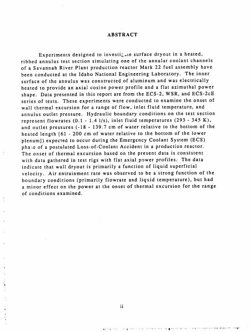
ABSTRACT

Experiments designed to investig.,te surface dryout in a heated,ribbed annulus test section simulating one of the annular coolant channels

of a Savannah River Plant production reactor Mark 22 fuel assembly have

been conducted at the Idaho National Engineering Laboratory. The innersurface of the annulus was constructed of aluminum and was electrically

heated to provide an axial cosine power profile and a flat azimuthal power

shape. Data presented in this report are from the ECS-2, WSR, and ECS-2cEseries of tests. These experiments were conducted to examine the onset ofwall thermal excursion for a range of flow, inlet fluid temperature, and

annulus outlet pressure. Hydraulic boundary conditions on the test section

represent flowrates (0.1 - 1.4 l/s), inlet fluid temperatures (293 - 345 K),

and outlet pressures (-18 - 139.7 cm of water relative to the bottom of the

heated length [61 - 200 cm of water relative to the bottom of the lower

plenum]) expected to occur during the Emergency Coolant System (ECS)

pha',e of a postulated Loss-of-Coolant Accident in a production reactor.The onset of thermal excursion based on the present data is consistent

with data gathered in test rigs with flat axial power profiles. The data

indicate that wall dryout is primarily a function of liquid superficial

velocity. Air entrainment rate was observed to be a strong function of the

boundary conditions (primarily flowrate and liquid temperature), but hada minor effect on the power at the onset of thermal excursion for the rangeof conditions examined.

_

ii

' ' I_"I '" ,r'll ' ' I rl .... _r, ,', '" *, ,,p,r _,ipl,, ,,, s rl,l,r i,,,I , ,irl q ,r,,,,li,PiiF, rip ,, rl_l r, IlqllIll ii ,'l', ' ',HIII_I"

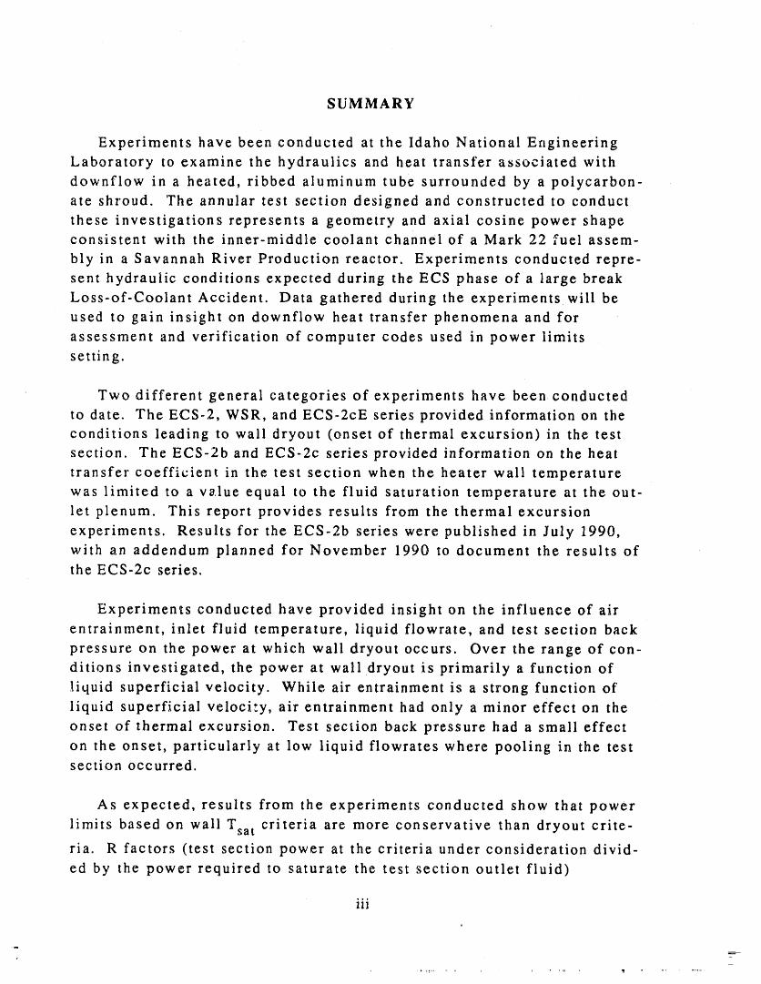
SUMMARY

Experiments have been conducted at the Idaho National Engineering

Laboratory to examine the hydraulics and heat transfer associated with

downflow in a heated, ribbed aluminum tube surrounded by a polycarbon-ate shroud. The annular test section designed and constructed to conduct

these investigations represents a geometry and axial cosine power shapeconsistent with the inner-middle coolant channel of a Mark 22 fuel assem-

bly in a Savannah River Production reactor. Experiments conducted repre-

sent hydraulic conditions expected during the ECS phase of a large break

Loss-of-Coolant Accident. Data gathered during the experiments will be

used to gain insight on downflow heat transfer phenomena and for

assessment and verification of computer codes used in power limitssetting.

Two different general categories of experiments have been conducted

to date. TheECS-2, WSR, andECS-2cE series provided information on the

conditions leading to wall dryout (onset of thermal excursion) in the test

section, The ECS-2b and ECS-2c series provided information on the heat

transfer coefficient in the test section when the heater wall temperature

was limited to a va.lue equal to the fluid saturation temperature at the out-

let plenum. This report provides results from the thermal excursion

experiments. Results for the ECS-2b series were published in July 1990,with an addendum planned for November 1990 to document the results ofthe ECS-2c series.

Experiments conducted have provided insight on the influence of air

entrainment, inlet fluid temperature, liquid flowrate, and test section back

pressure on the power at which wall dryout occurs. Over the range of con-ditions investigated, the power at wall dryout is primarily a function of

liquid superficial velocity. While air entrainment is a strong function of

liquid superficial velocity, air entrainment had only a minor effect on the

onset of thermal excursion. Test section back pressure had a small effect

on the onset, particularly at low liquid flowrates where pooling in the testsection occurred.

As expected, results from the experiments conducted show that power

limits based on wall Tsa t criteria are more conservative than dryout crite-

ria. R factors (test section power at the criteria under consideration divid-

ed by the power required to saturate the test section outlet fluid)

iii

i,1 ,i i _1 ,],]1 i_ _,1 _,llll i

I, , ,_, , k' ..... k. _ ,_h.J.,

calculated using wall Tsa t criteria are approximately one-half those calcu-

lated using the thermal excursion (dryout) criteria.

I)ata collected from the INEL experiments are in basic agreement with

data reported from test facilities using heaters with flat axial power

profiles. For the superficial velocity range of major interest (0.3 to 0.8

m/s), R factors obtained from ECS-2 experiments are approximately 15%

lower than those obtained from Westinghouse Savannah River Company

(WSRC) experiments. This result was expected since for an equivalent

power, the ECS-2 system had higher heat fluxes relative to the WSRC sys-tems and heat flux is an important factor in dryout phenomena.

- iv

ACKNO WL EDG EM E NTS

Many people contributed to the success of the experiments reported in

the following pages. B. R. Merkley kept the facility hardware operating. P.

R. Schwiederand J. R. Boyce solved the electronics mysteries. We are

indebted torteN. Romero for operation of the video system. 13. R. Merkley,

J. R. Boyce, H. N. Romero, and J. M. Hopla helped conduct the experiments.

z

V

CONTENTS

ABSTRACT ....... . ............................. ................... ii

SUMMARY .................................. .......... , .......... iii

ACKNOWLEDGEMENT .............................................. . v

1. INTRODUCTION .................................. ............... 1

2. FACILITY DESCRIPTION .......................................... 4

2.1 Loop Description ........................................... 4

2,1.1 Loop Instrumentation ................................. 6

2.2 Test Section Description .................................... . 7

2.2.1 Composite Heater .................................... 10

• 2.2.2 Plena and Shroud ................................... 15

2.2.3 Test Section Instrumentation. 15

2.2 4 Data Acquisition System ............................. 18

3. EXPERIMENT DESCRIPTION ...................................... 21

3 1 Checkout Tests ........................................... 21

3.1.1 Measurement Verification. ........................... 21

3.1.2 System Operational (SO) Test ......................... 22

3.1.3 Air Power Pulse and Liquid Full Checkout Tests ........ 22

3.2 Routine Data Integrity Checks ............................... 23

3.3 Experimental Procedure .................................... 24¢,

3.4 "rest Matrix .............................................. 26

4. RESULTS 30

4.1 Typical Test Results ....................................... 30

: 4.1.1 Wall Temperatures .................................. 32

4.1.2 Pressures and Differential Pressures ................... 35

_ 4.1.3 Fluid Temperatures .................................. 40

4.1.4 Air Entrainment .................................... 43

4.1.5 Azimuthal Wall Temperature Variation ................. 44

m

vi=

__

4.2 Overall Test Results ........................................ 46

4.2.1 Inlet Flow Rate ..................................... 48

4.2.2 Inlet Liquid Temperature ............................ 55

4.2.3 Standpipe Setting ................................... 57

4.2.4 Simple Data Correlation .............................. 58

4.2.5 Facility and Operational Influence on

Saturation Ratio ..................................... 63

4.3 Comparison of Excursion Criteria and Wall Saturation

Criteria ..... .... . ........................................ 66

5. CONCLUSIONS .................... .............................. 70

6. REFERENCES ................................................... 73

Appendix A" Engineering Drawings for the ECS-2 Test Fixture ........ A-1

Appendix B" Measurements Lists for t_e, ECS-2 and ECS-2c

Thermal Excursion Experiments ........................ B-1

Appendix C: Measurement Uncertainty for theECS-2Thermal Excursion Tests .............................. C-1

Appendix D ° Calculations Supporting Design/Performance of theECS-2 Inner Heater ................................... D-1

AppendixE: Calculated Parameters for the ECS-2 and ECS-2c

Thermal Excursion Experiments ........................ E-1

AppendixF: Data Repeatability for Onset of Thermal

Excursion Experiments ..................... ........... F- 1

• Appendix G" ECS-2 Air Ingress Test Results ......................... G-1

Appendix H" Video System Used During the ECS-2 ThermalExcursion Tests. H- 1

" vii

Appendix I' Questionable or Failed Measurements for theECS-2 and ECS-2c Thermal Excursion Experiments ........ I-1

Appendix J" Experimental Data Summary for INEL ThermalExcursion Tests (ECS-2, WSR, and ECS-2cE Tests) .......... J-1

,,

FIGURES

2. ,1. ECS-2 loop schematic ..... ,..................................... 5

2.2. ECS-2 test section ......... . ............... 8

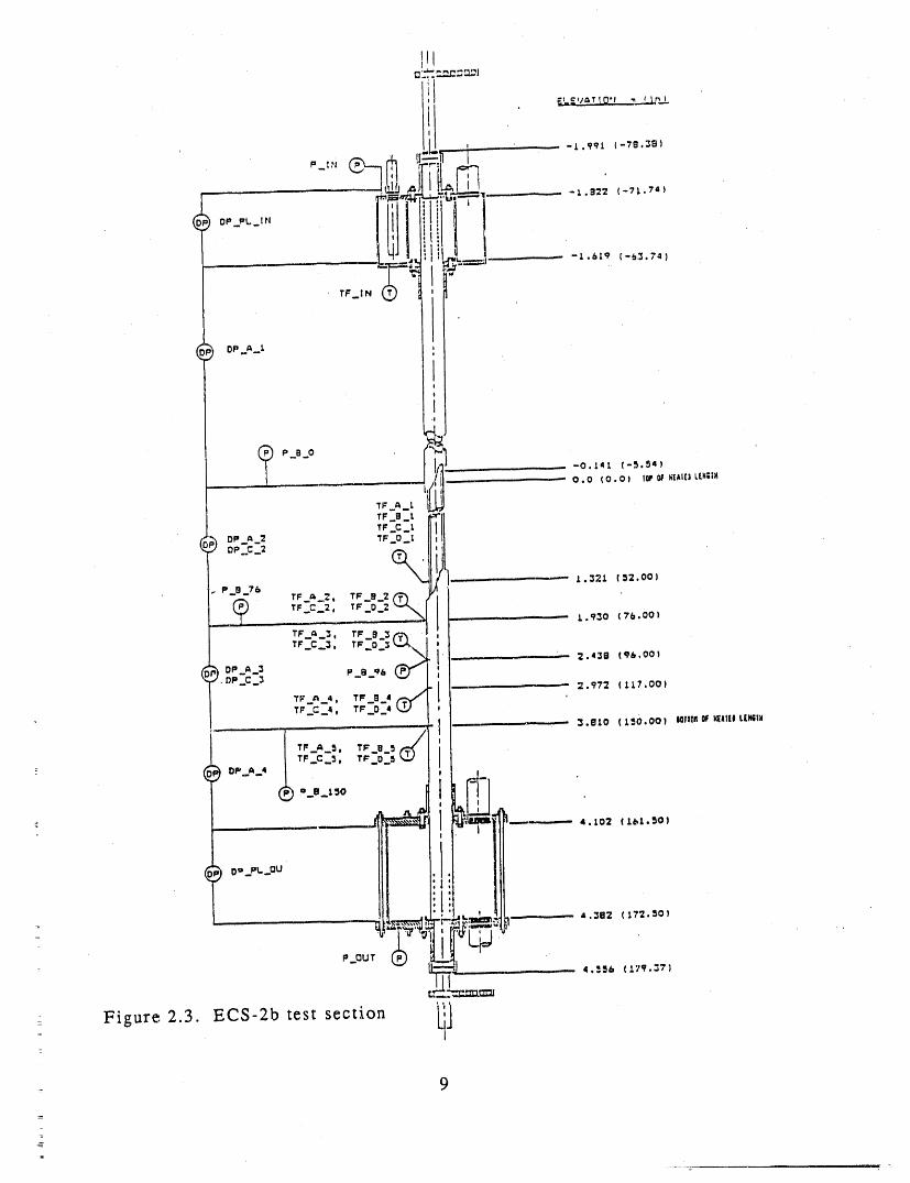
2.3. ECS-2b test section. 9

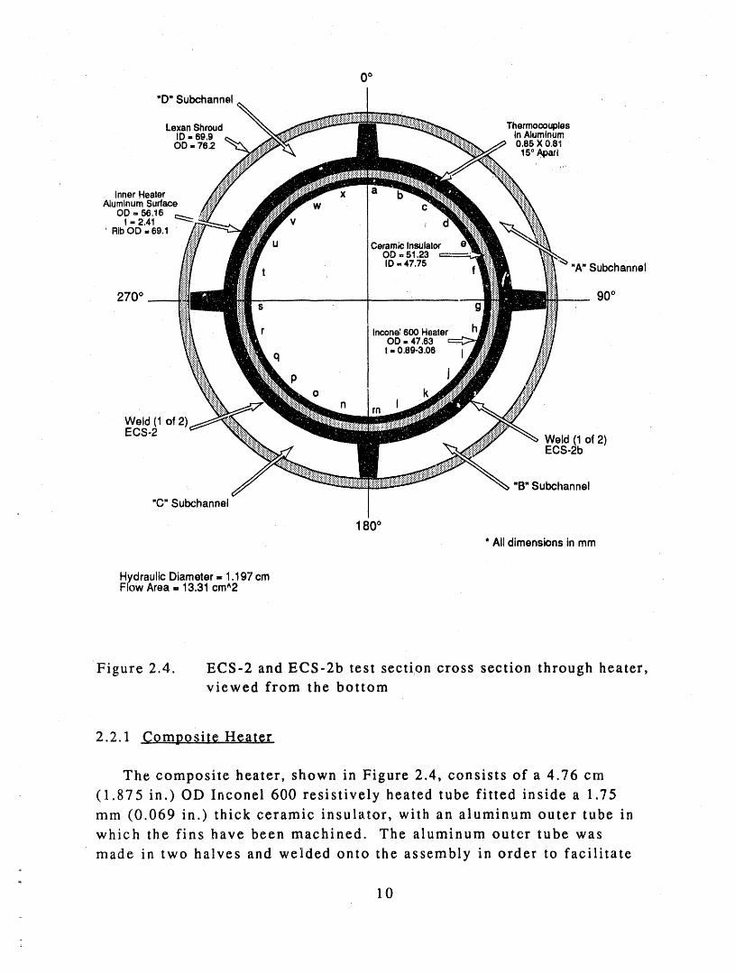
2.4. ECS-2 and ECS-2b test section cross section through heater,viewed from the bottom ..................................... 10

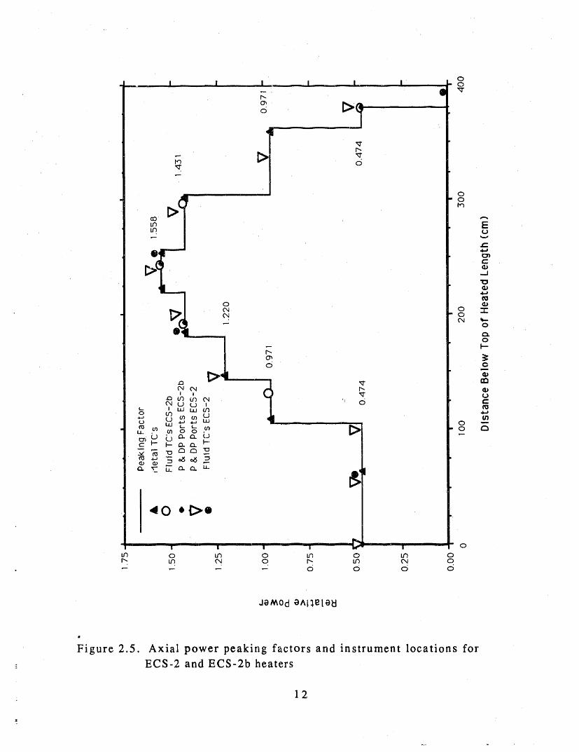
2.5. Axial power power peaking factors and instrument locationsfor ECS-2 and ECS-2b heaters ................................. 12

2.6. ECS-2 andECS-2b aluminum tube cross section .................. 14

4.1. Comparison of electrical and thermal power for ECS-2BL_5 ....... 31

4.2. Time history of level 7 wall thermocouple and power. 32

4.3. Full time history of ali level 7 thermocouples tor ECS-2BL_5 ...... 33=

= 4.4. Expanded time scalecc, mparison of level 7 thermocouplesfor ECS-2BL_5 34

4.5. Wall thermocouple response in B subchannel forECS-2BL_5 ...... 35

4.6. Comparison of inlet and outlet plenum pressures with

local atmospheric pressure for Test ECS-2BL_5 .................. 36

4.7. Inlet and outlet plenum levels for ECS-2BL_5 ................... 36

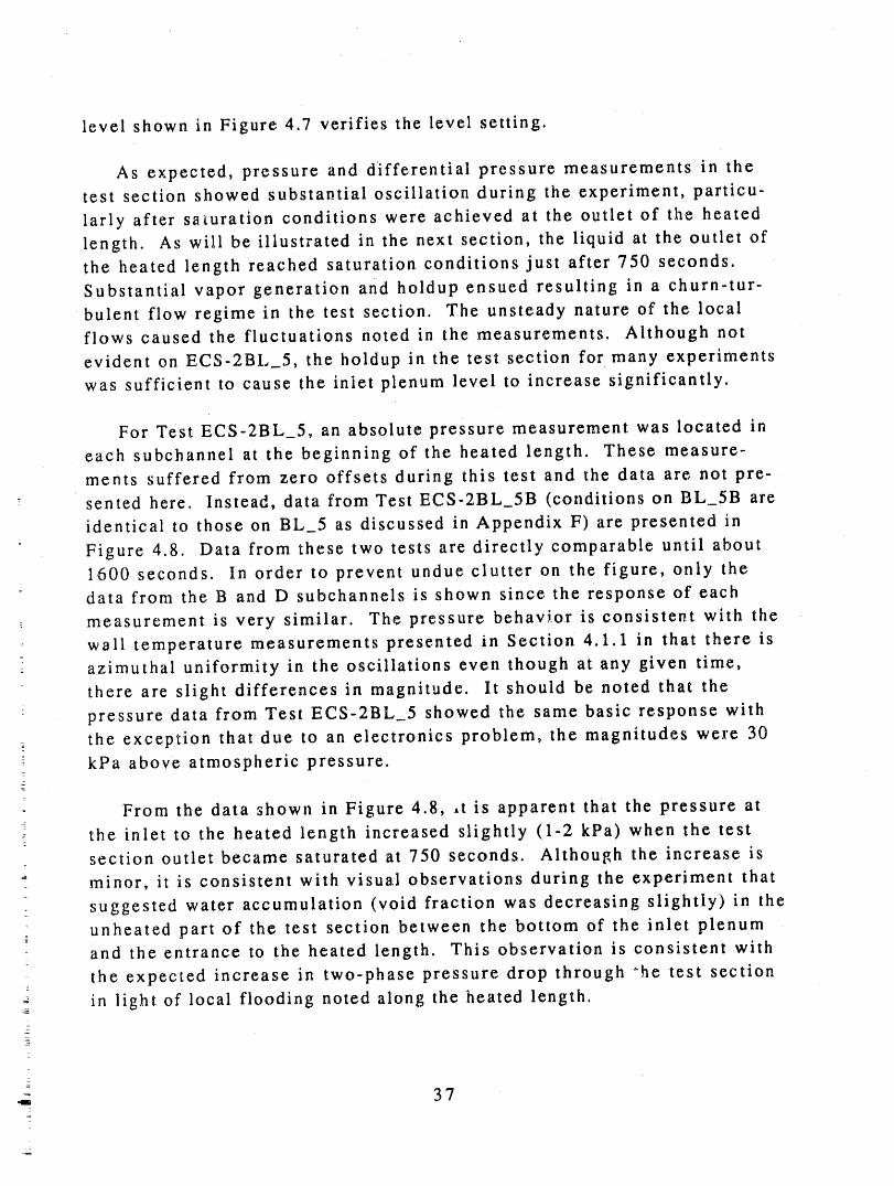
4.8. Comparison of subchannel pressure measurements at the

- entrance to the heated length for Test ECS-2BL_5B .............. 38

viii_

_

4.9. Differential pressures in upper half of the heated lengthfor Test ECS-2BL_5 ............ .............................. 39

4.10. Differential pressures in the lower half of the heated lengthfor Test ECS-2BL_5, 40

4.11. Plenum and heated length outlet fluid temperaturesfor Test ECS-2BL_5 ......................................... 41

4.12. Axial fluid temperature distribution for Test ECS-2BL_5 ......... 42

4.13. Comparison of fluid thermocouples at 257 cm for TestECI;-2BL._5 . 43

4.14. Expanded time scale comparison of fluid temperaturesat 257 cm for Test ECS-2BL_5 44

4.15. Air inlet and outlet flowrates for Test ECS-2BI,_5 ............... 45

4.16. Azimuthal temperature distribution during power step

just prior to excursion power step for Test ECS-2BL_5 ............ 46

4.17. Azimuthal wall temperature distribution during power stepon which sustained excursion occurred for Test ECS-2BL_5 ....... 47i

4.18. Azimuthal fluid temperature distribution during power step

just prior to excursion power step for Test ECS-2BL_5 ........... 48

4.19. INEL thermal excursion data for 295-315 K inlet

temperature and 323-383 cm standpipe setting ................. 53

4.20. INEL thermal excursion data for three different inlet

temperatures and a ' standpipe setting of 389 cm ................ 55

4.21. INEL thermal excursion data for 326 K inlet temperature

with standpipe setting as a parameter ......................... 57

4.22. INEL thermal excursion data with inlet temperature as a

parameter ................................................. 59

ix

4.23. INEL thermal excursion data with standpipe setting

as a parameter .............................................. 60

4.24. INELECS-2 andECS-2cE thermal excursion data with

power law fits ............................................... 61

4.25. INEL thermal excursion data compared to

Duffey,Hughes model ..... .................................. 64

4.26. INEL thermal excursion data with test facility

as a parameter ...... .... 65

4.27. Thermal excursion data from several sources and INEL

Wall saturation data .......................................... 68

TABLES

2.1. Inconel 600 heater information 13

2.2. Location of wall thermocouples forECS-2 heater .................. 19

2.3. Location of wall thermocouples forECS-2b heater ............... 20

3.1. Range of parameters for thermal excursion experiments .......... 26

3_2. Nominal conditions for excursion tests conducted in the

ECS-2 facility 27

3.3 Nominal conditions for excursion tests conducted in

the ECS-2b facility 28

4.1. Statistics for aluminum wall temperatures for pre-excursion

power step on Test ECS-2BL 5 (2210-2230 s time frame) ........ 49

4.2. Statistics for aluminum wall temperatures on excursion

power step on Test ECS-2BL_5 (2340-2360 s time frame) ........ 50

4.3. Statistics results for test section flui6 temperatures on Test

ECS-2BL_5 pre-excursion power step (2210 to 2230 s) ........... 51

X

4.4. Summary of results from INEL ECS-2 and WSR thermal

excursion experiments .................... ................... 52

4,5. Summary of results froro INEL ECS-2cE thermal excursionexperiments , 53

4,6. Power fit constants for Equation 4-1 using inlet

temperature data sets ....................................... 61

4.7. Influence of 520 K and 620 K wall temperature criteria on

saturation ratio for INEL thermal excursion data points .......... 67

xi

1. INTRODUCTION

In mid 1987, the U.S. Department of Energy (DOE) initiated a vigorous

program to review the safety and operation of the nuclear materials

production and nuclear testing facilities under DOE management in the U.S.A major purpose of this ongoing review effort is to ensure that the

facilities in the existing research and weapons materials production

complex are operated in a safe manner during normal operation and, given

a hypothetical design basis accident, the risk to the public is within

acceptable limits.

As part of this review effort, Westinghouse Savannah River Company

(WSRC) personnel have conducted or contracted researchto examine heattransfer in the Savannah River Plant (SRP) reactor fuel assembly during

the Emergency Cooling System (ECS) phase of a hypothesized Loss-of-Cool-

ant Accident (LOCA). During the ECS phase of the accident, the reactor fuel

assemblies are expected to be filled with a two-phase air-water mixture.

Safety requirements dictate that the power levels be low enough during

the ECS phase of the accident so that no melting occurs in the fuel assem-blies.

Two different criteria, wall saturation temperature and wall dryout,

are being considered for use in calculating power limits. Simply stated,

wall saturation temperature criterion involves determining the power for a

given thermal-hydraulic condition (flowrate, inlet fluid temperature, etc)

at which the maximum assembly wall temperature just reaches the local

saturation temperature. This criterion would preclude bulk boiling of the

liquid in the assemblies. The dryout criterion involves determining the

pc cer at which heat transfer from the surface of the heated assembly wall

degrades to a point where the surface is basically dry and the wall

temperature starts to increase in a nearly adiabatic fashion. Of the two

criteria, wall saturation is the considerably more conservative.

Complex geometry and hydraulic interactions involving air: entrainment, flooding, and heat transfer to two-phase mixtures necessitate

experimental investigation of the processes involved to help determine

key factors influencing assembly cooling and hence the power limit

criteria. Research results from such investigations will be used in the

verification and assessment of models used for establishing acceptable

power limits for the reactors.

= 1- /

Experimental efforts conducted at the Savannah River Site (SRS) HeatTran._fer Laboratory to examine ECS power limits are reviewed by Steimke

[I]. Prior to 1988, experiments _vere conducted in an annulus consisting ofa hea:ed stainless s_eel surface (rather than aluminum as in actual fuel_

assemblies) and glass or alum:,num as the other wall of the annulus [2; 3].Stainless steel was used as lhc heated s_,rface because of technical difficul-

ties associated with resistively heating aluminum to the power levels re-

quir_.d for the desired experiments. These facilities did not contain axial

spacer ribs in the an_uluT,, a unique feature of the reactor assembly design.

Also, these test section_ used a flat axial power profile and uniform azi-

i mu_hal powel. FL:ilities .'hat included spacer ribs and an azimuthal powertilt were constructed in 1988 [_.;5;6]. Other facilities were built in 1989 [7]

for visualization studies and to incorporate thermal spray technology forthe construction of aluminum heated surf;ees [8; 9]. Ali test sections men-

tioned above incorporated a flat axial power profile (the FB rig had an azi-

muthal power tilt)and with the exception of two test sections, used stain-

less steel for the heated surface. Although, both of the thermal sprayed

_est sections used aluminum for the heated surface, current technology al-

lowed only the outer annulus wall to be heated.

The ECS-1 facility [10] was constructed and operated at the Idaho Na-

tional Engineering Laboratory (INEL) in 1989 to help address the

influences of heater surface material properties and conditions on test re-

suits. TheECS-I facility was sponsored by the Department of Energy, Of-

fice of Safety Appraisal, Environment Safety and Health and consisted of a

ribbed aluminum tube heated from inside with a resistively heated stain-

less steel tube and surrounded by a Lexan ru shroud to permit visual obser-

" vation. Nearly 50 experiments were conducted to examine the effects ofair entrainment, flow regime transition, flow distribution, and flooding on

" the heat transfer processes in the annulus.

The s_c, cess of the heater design used in the ECS-1 facility prompted

the constructio_ of theECS-2 facility at the INEL. The ECS-2program was

sponsored by the WSRC and incorporated several improvements relative to

the ECS-1 fixture. Foremost was a new inner heater with an axial power

profile consistent with the power shape to be used in setting assembly

power limits and improvements in the inlet and outlet geometry of the testsection to make the plenums more prototypic. The ECS-2b facility

succeeded the ECS-2 facility. With the exception of measurement locations

2

and a new heater, the two facilities were essen',ially the same.

Two different categories of experiments were ru, during the course of

the INEL ECS-2program. More than 70 experiments (the ECS-2b, and ECS-

2c series) were conducted to determine the hydraulic conditions that lead

to heater wall temperatures that just exceed local fluid saturation

temperature. Results from these experiments are discussed by Anderson,

et al [11]. Approximately 50 experiments (theECS-2, WSR, and ECS-2cE se-ries) were conducted to establish and examine the variables and conditions

that lead to sustained dryout on the heated surface in the annulus. Tests

conducted in these programs were designed to parametrically examine theinfluence of coolant temperature, coolant flowrate, and back pressure on

the heat transfer processes in the ribbed annulus. Data gathered will be

used to improve understanding of the physical processes involved and inthe assessment and validation of models used in the calculation of powerlimits criteria.

The remainder of this report details results of the thermal excursiontests conducted at the INEL. Results discussed are from the ECS-2, WSR,

and ECS-2cE series of experiments conducted irl the ECS-2 and ECS-2b

facilities. Section 2 describes facility design, support systems, measure-

ment capabilities, and the data acquisition system. Experiment conduct

and test matrices are addressed in Section 3. Results of the experimental

investigations are presented in Section 4. Conclusions and summary state-

ments are given in Section 5. Appendices to this report provide engineer-

ing drawings, lists of measurements recorded for the various experiments,

measurement uncertainty statements, test fixture design details, and otherrelevant information.

.

_ld , ilil_ tj,,

2. FACILITY DESCRIPTION

This section describes the test facility, support systems,

instromentation, and data acquisition system. As noted above, the ex-

periments described in this report were conducted in the ECS-2 andECS-2bfacilities. In most respects, theECS-2 andECS-2b facilities are

similar. In fact, theECS-2b test section is actually made up from the

upper and lower plenums and shroud from the ECS-2 test section and aheater that was intended for the dual heated annulus program. The t

dual heated inner heater is t!,e same design as the ECS-2 heater with

slight changes to simplify and improve the fabrication of the heater.

Major differences between the ECS-2 and ECS-2b facilities include thenumber and location of the test section fluid temperature, absolute

pres-z,_re, and differential pressure measurements and the location of

the heater wall thermocouples. Since the ECS-2b facility geometry isdescribed by Anderson [11], the description in this report is limited pri-

marily to the ECS-2 hardware.

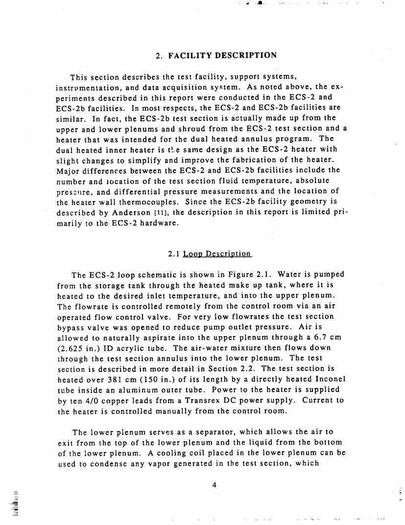
2.1 L__q_Qg_D__cription

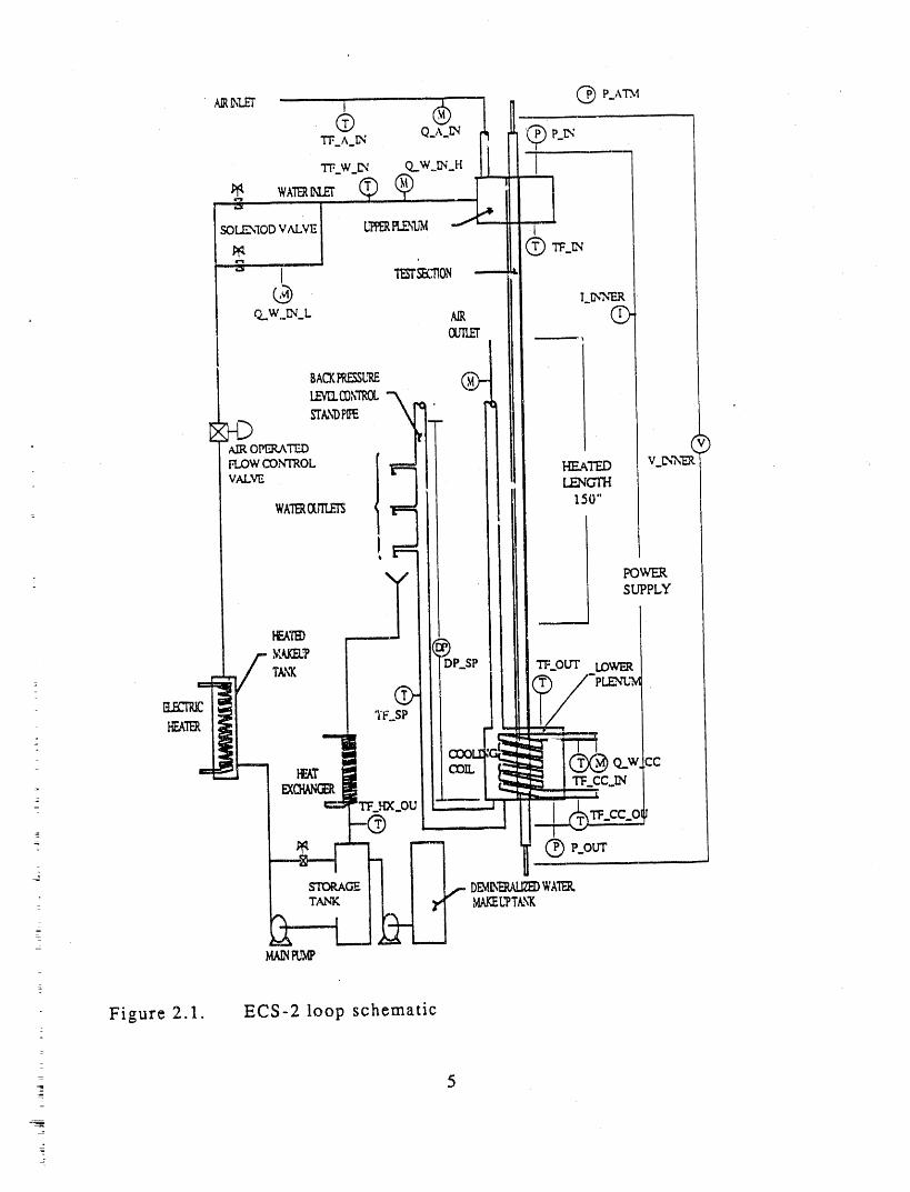
TheECS-21oop schematic is shown in Figure 2.1. Water is pumped

from the storage tank through the heated make up tank, where it isheated to the desired inlet temperature, and into the upper plenum.

The flowrate is controlled remotely from the control room via an air

operated flow control valve. For very low flowrates the test section

bypass valve was opened to reduce pump outlet pressure. Air isallowed to naturally aspirate into the upper plenum through a 6.7 cm

(2.625 in.) ID acrylic tube. The air-water mixture then flows down

through the test section annulus into the lower plenum. The testsection is described in more detail in Section 2.2. The test section is

heated over 381 cm (150 in.) of its length by a directly heated Inconeltube inside an aluminum outer tube. Power to the heater is supplied

by ten 4/0 copper leads from a Transrex DC power supply. Current to

the heater is controlled manually from the control room.

The lower plenum serves as a separator, which allows the air to

exit from the top of the lower plenum and the liquid from the bottom

of the lower plenum. A cooling coil placed in the lower plenum can be

used to condense any vapor generated in the test section, which

,_____ Q P_A"D,'I

@ Q_,,:_ ® _,t',,"W_A_IN i i -

w_w__ Q..W.._'_H I I

* , IL 1_,., . . _-_

_--_ --(_ T_TION ,I I _,,,'NF_.R"

_w___t. AIR @ou2zr ii i

_,','TROL "X - _L II

,_ or,_'r_ II II . v)FLOWCO,N'IROL

= WATER_ ! 150"

. POWERSUPPLY

_ _-_ -o_ ___' DE__ WAT_

MANI_NP

Figure 2.1. ECS-2 loop schematic

r

z

_ 5-

prevents the vapor from exiting through the outlet air measurementstation. The water flows from the outlet tap through a heat exchanger

and back into the storage tank completing the loop. The loop inventory

is supplied by water from the demineralized water tank. The liquidlevel in the test section is controlled by the height of the water outlet

taps located in the back pressure level control standpipe. For theexcursion test series, these levels were -18, 0, 19, 48, 51, 110, and 140

cm (-7, 0, 7.5, 19, 20, 43, and 55 in.) above the bottom of the heated

length.

2.1.1 Loop Instrumentation_

Sufficient loop instrumentation is provided to control and monitor

inlet conditions to satisfy program ot, jectives and to calculate a test

section energy balance. (A listing of ali instrumentation for the ECS-2

and ECS-2b test sections is provided in Appendix B). The energy

balance is monitored continuously on line to provide an overall

integrity check and to determine when the system has reached steady

state conditions following a change in power or flowrate. Ali fluid

thermocouples are 1.5-mm (0.060-in.) type K stainless steel sheathed

with a grounded junction inserted directly into the fluid stream. They

are connected to type K extension wire which runs to a 339 K (150°F)

reference oven. Regular copper conductors are used to connect the

ovens to the data acquisition system (DAS).

The air inlet and outlet flowrates (Q.A_IN and Q_A_OUT) are

measured using Teledyne/Hastings model LU-3M mass flow meters

having a measurement range of 0-50 standard liters per minute

(SLPM). These are very low pressure drop instruments having aninternal diameter of about 6 cm (2.5 in.). The inlet and outlet air tem-

peratures (TF_A_IN and TF_A_OUT) were measured using fluid

thermocouples as described above. _oth a high flow (Q_W_IN_H) and a

low flow (Q_W_IN_L) turbine meter were used to measure the inlet

liquid flow. Flowrates below 0.30 l/s were routed through both

turbine meters. For flowrates above 0.30 l/s, only the high flow

turbine was used. The liqui6 inlet temperature tTF_W_IN) was

measured using a fluid th_:rmocouple and was checked regularly

against a calibrated glass thermometer inserted into the inlet liquid

stream. The inlet liquid temperature was controlled by adjusting the

i heat input to the heated makeup tank. No outlet liquid flowrate

6

measurements were made and the liquid outlet temperature was

measured using a fluid thermocouple (TF_W_OUT for ECS-2 and TF_SP

forECS-2b). The inlet (TF_IN) and outlet (TF_OUT) plenum

temperatures were also measured using fluid thermocouples. The inlet

(P_IN) and outlet (P_OUT) plenum absolute pressures were measured

using Sensotec absolute pressure transducers. The liquid temperatureat the outlet of the heat exchanger (TF_HX_OUT) was measured using a

fluid thermocouple. The liquid level ira the level control standpipe was

measured using a differential pressure cell (DP_SP) connected betweenthe bottom of the lower plenum and a point above the highest outlet

tap. During testing, the storage tank temperature was monitored tohelp determine the necessary secondary heat exchanger flowrate butwas not recorded. The water flowrate (Q_W_CC) through the lower

plenum cooling coil was measured using a turbine flowmeter and the

inlet (TF_CC_IN) and the outlet (TF_CC._OU) temperatures were

measured using fluid thermocouples.

The test section voltage (V_INNER) was measured w,_'th _ volt meter

connected directly across the test section. The current through the test

section (I_INNER) was determined by measuring the voltage across acurrent shunt of known resistance.

Local atmospheric pressure (P_ATM) was ;.neasured using aSensotec electronic barometer and was checked daily against the

atmospheric pressure recorded at the INEL Standards and Calibration

Laboratory.

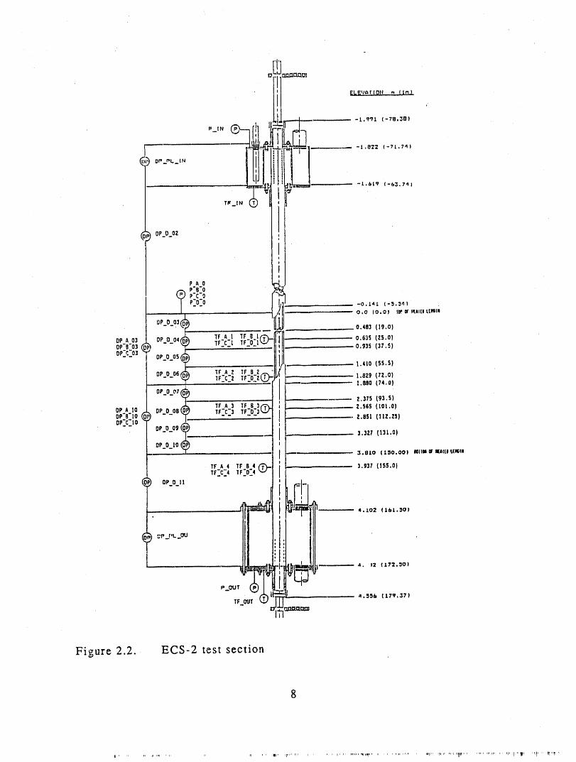
2.2 Test S_¢_ion Description

For this discussion the test section is defined as the upper and

lower plenums, the connecting transparent shroud, and the composite

heater. Figure 2.2 shows the ECS-2 test section with pertinentelevations indicated on the right side and instrumentation designations

on the left side. A companion figure for the ECS-2b test section is

shown in Figure 2.3 and is discussed by Anderson[;,1]. Instrument_'.tion

: on the composite heater is not shown on this figure. A cross section

view through the heated portion of the test section for ECS-2b is shown

in Figure 2.4. Note that the heater for ECS-2 is essentially the same ex-

_ cept that welds on the ECS-2 heater are in the A and C subchannels.

- 7

-- -l."_ (-7t.74)

___. -- -1.6L? (-6:3.7411

OP.O_OZ

I, 0

i

P_O Ii

P-8"O

P-o-o _ -o._4L (-_,_4_____ --- 0=0 (0.0| tO_ Of i_.IU(I LtRgIN

°P-°-O_(_ o.4. 119.o)

TF A | TF O I_-___ 0.63S (Z5,O)oPAo:3 Dr0 04__) Tr'C'l TF'O-I',:-.'0P'6-03 _ - - _ _ _ - -. 0,935 (37.S)

op.<'o,_oi,_o_os_._ i -l.,,o(ss.'_)oPoo,5_) ',F,z _,,2-- TF"C_'.Z TF-O'_2(_ |.829 (7Z.O)

LC _ [.880 (74. LI)OP 0_07(_ ,, , , 2.375 (93.S)

TFA,_'F8_r_ ' 2.sss(lol.o)oP'B'to(__ ...... z.ssl(I,z.zs)m,'c'Io ',

- - o_.o_o9(__ -- I_" :3.'.,,7(:3,.o)o,,._o_lo(_

.... I =.sLoc_so.oo_..= or..e. t_,.

TFA_ ;_tS_ ] _.gsz(tss.oITF._C"4 TFZO"4!

__r i_ _" 4.102 (16L.:)01!

-" !i

.=,,® IUT

•-11====

Figure 2.2. ECS-2 test section

,,,li,' .,, .... I_'qlll"......... ""_'r.... i'_lrlIr'l'II_a 'ql' I_"1'I1

I

o.o (o.o_ Iuo_.tA_.Lt_;;H

TF _ --L I

TF_B t _.

,__cL Iiiop.c_z - -

. P__B7_ _- " 1.321 f52.00)

TF _C 2,

TF_C_3,

.oP_c_3 F,s_,

r_-.a_,. ,,___,(_l,,,,,"j ....... =.,,= ,:_,.oo,TF_C_4, TF _D 4 f

TF.A 5, TF" B ,_ (_

i

" B..t 50e'=-l--

¢ A ' I, _ ,

Figure 2.3. ECS-2b test section '}jI

0

"D" Subchannel

LexanShroud ThermoooupleslD= 69.9 in AluminumOD= 76.2 0.85 X 0,81

InnerHeaterAluminumSurface W C

OD = 56,16t = 2,4'1 _ V I

' RibOD = 69.1

U Ceram;cInsulalor eOD,,,51.23lD - 47.75 "A" Subchannelt f

270 ° 90 °s - g ,

r Inconet600 Heater hOD. 47.63

q t. 0,89-3.06 I

p Jo k

Weld (1 of 2)

ECS-2 Weld (1 of 2)EOS-2b

"B" Subchannel

"C" Subchannel

1800* Ali dimensions in mm

Hydraulic Diameter = 1.197 cmFlow Area = 13.31 cre^2

Figure 2.4. ECS-2 and ECS-2b test section cross section through heater,viewed from the bottom

2.2.1 Composite Heater

The composite heater, shown in Figure 2.4, consists of a 4.76 cm

(1.875 in.) OD Inconel 600 resistively heated tube fitted inside a 1.75

mm (0.069 in.) thick ceramic insulator, with an aluminum outer tube inwhich the fins have been machined. The aluminum outer tube was

made in two halves and welded onto the assembly in order to facilitate

=

10

fabrication. Power leads through the unheated portion of the heater

were made of copper tubing (wall thickness of 8.59 rnm [0.338 in.])

brazed to the ends of the Inconel heater tube. The composite he_er

was fabricated by sliding the ceramic insulator over the inconel t(abe,

placing the two aluminum halves over the insulator, and then TIG

welding the aluminum halves together longitudinally, with the weldsin subchannels B & D on the ECS-2b heater and in subchannels A & C

on the ECS-2 heater. As the weld cooled, the composite was drawn

tightly together. The weld surface was then dressed to the basic tube

diameter. The completed assembly for ECS-2 is shown in Drawing

429994 in Appendix A.

The Inconel heater tube was fabricated by welding together eight

sections of Inconel 600 tubing of various lengths having five different

wall thicknesses in order to produce the axial power profile shown in

= Figure 2.5. Information for each section is presented in Table 2.1. The

sections were welded together using an Astro Arc automatic tube

welder. No welding filler material was required with this automatic.

welder. Several sample pieces for each of the weld joint thickness

were made and destructively examined to determine the proper

welder settings to ensure a full penetration and uniform weld for each

joint. The copper power leads were then brazed to each end of the

Inconel tube. The completed assembly is shown in Drawing 430437 in

Appendix A. The completed assembly was then hung vertically in air

and power leads attached to the copper leads and a thermocouple was

attached in the center of each power zone. Power was applied to tileheater until the hottest zone reached 800 K (1000°F). This maximum

temperature was maintained for approximately one-half hour. The-

temperature profile was similar to the desired power profile indicatingthe correct sequence of heater sections. Any weld voids would show

up as dark spots in the welded zone. None were found. The electrical

resistance of the heaters were calculated from the voltage and currentmeasurements to be 0.0206 ohm for both the ECS-2 and ECS-2b heat-

ers. This was within 5% of the expected resistance calculated from the

tube lengths and thicknesses and the published resistivity for Inconel.

The Macor machinable ceramic was purchased as cylinders slightly

larger than 5 cm (2 in.) in diameter and approximately 15-cre (6-in.) in

length. Each cylinder was machined to an inside diameter of 4.78-cm

(1.880-in.) and an outside diameter of 5.12-cm (2.017-in.).

11

Ja_AOd aA}_Ia_

Figure 2.5. Axial power peaking factors and instrument locations forECS-2 and ECS-2b heaters

12

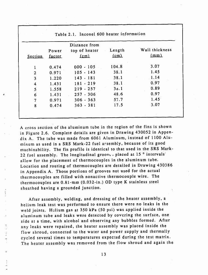
Table 2.1. Inconel 600 heater informat'ion

Distance from

Power top of heater Length Wall thickness

_S._e,_q.tJ_o._ factor _ Lfd!!.k (mm)

1 0.474 000 - 105 104.8 3.07

2 0.971 105 - 143 38.1 1.45

3 1.220 143 - !81 38.1 1.14

4 1.431 181 - 219 38.1 0.97

5 i.558 219 257 36.1 0.89

6 1.431 257 - 306 48.6 0.97

7 0.971 306 - 363 57.7 1.45

8 0.474 363- 381 17.5 3.07

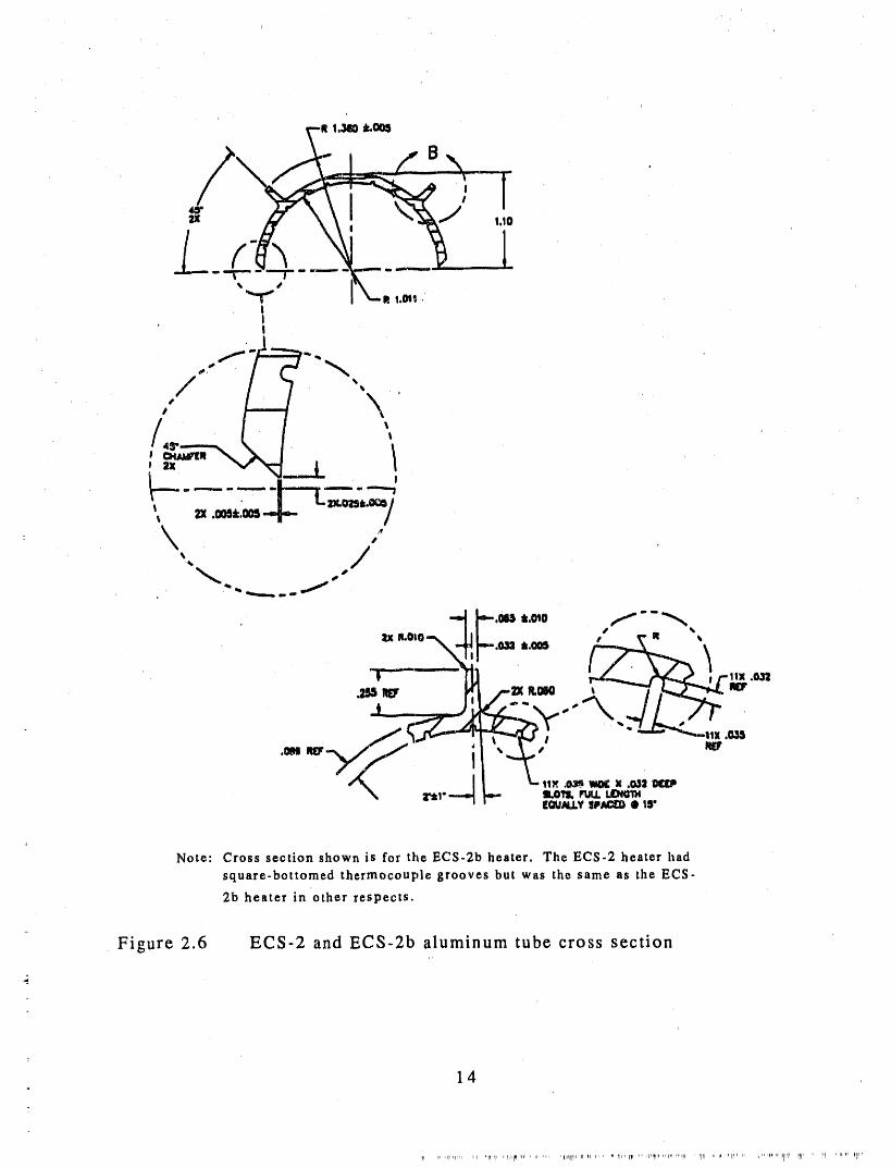
A cross section of the aluminum tube in the region of the fins is shown

in Figure 2.6. Complete details are given in Drawing 430052 in Appen-dix A. The tube was made from 6061 Aluminum, instead of 1100 Alu-

minum as used in a SRS Mark-22 fuel arsembly, because of its good

machinability. The fin profile is identical to that used in the SRS Mark-

22 fuel assembly. The longitudinal groov_., placed at 15 o intervals _

allow for the placement of thermocouples in the aluminumtube.

Location and routing of thermocouples are detailed in Drawing 430386

in Appendix A. Those portions of grooves not used for the actual

thermocouples are filled with nonactive thermocouple wire. The

thermocouples are 0.81-rnm (0.032-in.) OD type K stainless steel

sheathed having a grounded junction.=

±

After assembly, welding, and dressing of the heater assembly, a

helium leak test was performed to ensure there were no leaks in the

weld joints. H,zlium gas at 350 kPa (50 psi) was applied inside thealuminum tube and leaks were detected by covering the surface, one

side at a time, with alcohol and observing any bubbles formed. After

any leaks were repaired, the heater assembly was placed inside theflow shroud, connected to the water and power supply and thermally

cycled several times to temperatures expected duringthe test matrix.

The heater assembly was removed from the flow shroud and again the

13=

_

==m|_ 9..oos

III

, \

__L_ ..... I---7--- ---_'

• /

-'II"._t._o _'-_lx Ik,OtO,-_ L ,. . _ /' _ DI _',_

Note: Cross section shown is for tile ECS-2b heater. The ECS-2 heater had

square-bottomed thermocouple grooves but was the same as the ECS-

2b heater in other respects.

=

Figure 2.6 ECS-2 and ECS-2b aluminum tube cross section.

14

_, 'q,r,p_, ' _, 'r1_l , r,,,inl lr , up ,rh 'llnll'p_ I1 II I, , n til,, i11 ,, iil,lll_ln, p_ ,ripq ' _rlll ,, r_ 'II _ ' q,'"'_'PqlIl'I_ II_' II ' _ " PII'

welds were checked for leaks using the same helium leak test

procedure. When convinced that no water could leak into the testsection internals, the outer surface of the aluminum was treated to

make it wettable by immersing the entire heater assembly in a bath of

dilute sodium hydroxide for approximately three minutes. Verification

of each thermocouple location was made by identifying each junction

using a heat gun applied to the heater surface.

As shown on the drawings in Appendix A, the ECS-2 test section

design included provisions for a 1.07 nam ID, 3.66 m long heater rod

that could be positioned off-center inside the composite heater. The

internal heater was incorporated to provide an azimuthal power tilt al-

though it was never used.

2.2.2 P lena and Shroud

The upper and lower plena were made from acrylic plastic to allowobservation of the interior and were designed to provide prototypical

elevations and flow resistances. The plenum assembly details are

shown in Drawings 430049 and 431747 in Appendix A. The outer flowshroud was made from an 8-cm (3.0-in.) OD polycarbonate tube.

Details of the outer shroud are shown in Drawihg 430050..

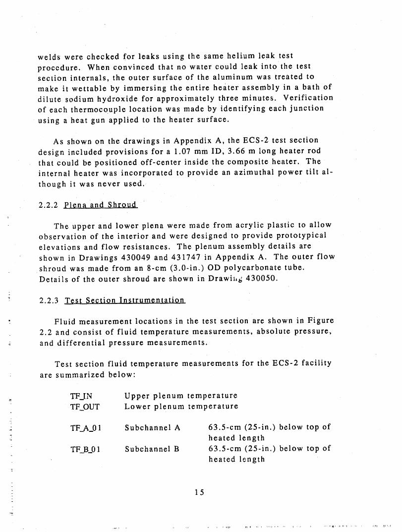
-- 2.2.3 Test Section Instrumentation_

• Fluid measurement locations in the test section are shown in Figure

2.2 and consist of fluid temperature measurements, absolute pressure,

and differential pressure measurements.

Test section fluid temperature measurements for the ECS-2 facilityare summarized below"

TF_IN Upper plenum temperature

TFOUT Lower plenum temperature-

TF_A._01 Subchannel A 63.5-cm (25-in.) below top of

- heated length

TF_B_01 Subchannel B 63.5-cm (25-in.) below top ofheated length

_

15_

=

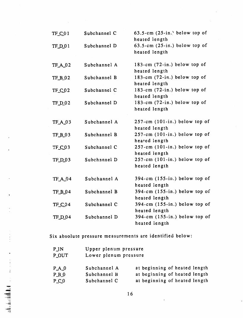
TF_C_01 Subchannel C 63.5-cm (25-in.) below top ofheated length

TF_D_01 Subchannel D 63.5-cm (25-in.) below top ofheated length

TF_A_02 Subchannel A 183-cm (72-in.) below top ofheated length

TF_B02 Subchannel B 183-cm (72-in.) below top ofheated length

TF._C_02 Subchannel C 183-cm (72-in.) below top ofheated length

TF_D_02 Subchannel D 183-cm (72-in.) below top ofheated length

TF_A_03 Subchannel A 257-cm (101-in.) below top ofheated length

TF_B._03 Subchannel B 257-cm (101-in.) below top ofheated length

. TF_C_.03 Subchannel C 257-cm (101-in.) below top ofheated length

TF_D._03 Subchannel D 257-cm (101-in.) below top of

heated length

TF_A_04 Subchannel A 394-cm (155-in.) below top ofheated length

TF_B_04 Subchannel B 394-cm (155-in.) below top ofI

heated length

TF_C._04 Subchannel C 394-cm (155-in.) below top ofheated length

TF_D_04 Subchannel D 394-cm (155-in.) below top of

heated length

Six absolute pressure measurements are identified below"

P_IN Upper plenum pressure" P_OUT Lower plenum pressure

P_A_0 Subchannel A at beginning of heated length

P_B_0 Subchannel B at beginning of heated length

P_C_0 Subchannel C at beginning of heated lengthi

16

m

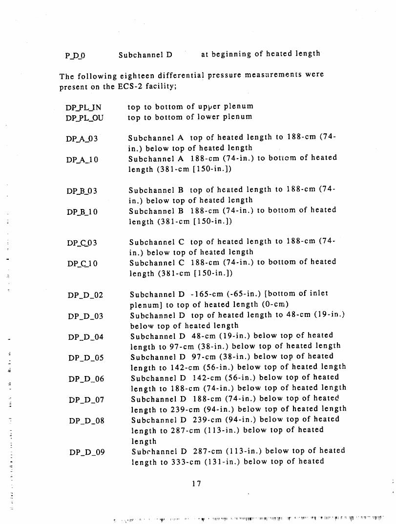
P_D_0 Subchannel D at beginning of heated length

The following eighteen differential pressure measurements were

present on the ECS-2 facility;

DP_PL_IN top to bottom of upper plenum

DP_PL_OU top to bottom of lower plenum

DP_A_03 Subchannel A top of heated length to 188-cm (74-

in.) below top of heated length

DP_A_10 Subchannel A 188-cm (74-in.) to bottem of heatedlength (381-cm [150-in.I)

DP_B_03 Subchannel B top of heated length to 188-cm (74-in.) below top of heated length

DP_B_IO Subchannel B 188-cm (74-in.) to bottom of heated

length (381-cm [150-in.])

DP_C_03 Subchannel C top of heated length to 188-cm (74-" in.) below top of heated length

DP_C_10 Subchannel C 188-cm (74-in.) to bottom of heated

_ length (381-cm [150-in.])

= DP_D_02 Subchannel D -165-cm (-65-in.) [bottom of inlet

plenum] to top of heated length (0-cm)

DP_D_03 Subchannel D top of heated length to 48-cm (19-in.)

below top of heated length

_ DP_D_04 Subchannel D 48-cm (19-in.) below top of heated

length to 97-cm (38-in.) below top of heated length

DP D_05 Subchannel D 97-cm (38-in.) below top of heated- w

= length to 142-cm (56-in.) below top of heated length

-: DP_D_06 Subchannel D 142-cm (56-in.) below top of heatedlength to 188-cm (74-in.) below top of heated length

DP D 07 Subchannel D 188-cm (74-in.) below top of heated_" length to 239-cm (94-in.) below top of heated length

Z DP_D_08 Subchannel D 239-cm (94-in.) below top of heated

_ length to 287-cm (113-in.) below top of heatedlength

DP_D_09 Subehannel D 287-cm (ll3-in.) below top of heated

length to 333-crn (131_in.) below top of heated-

17

_

_, ,,,l_tl,r' Irl ....... _lr r,lr, ............ Rill ' '"q"l'T_',,,,'_,rr 'r_ ',,1,1_ll]_lmrr,"_,m,_lllmll,,,iHrlll,_ll%lrl,_'p"" '_IlrllI''r'[ll'_ ]1[_19"'IIII IllI'1 ]lll_II I,II"lll"' I_lllllri'l'II'

length

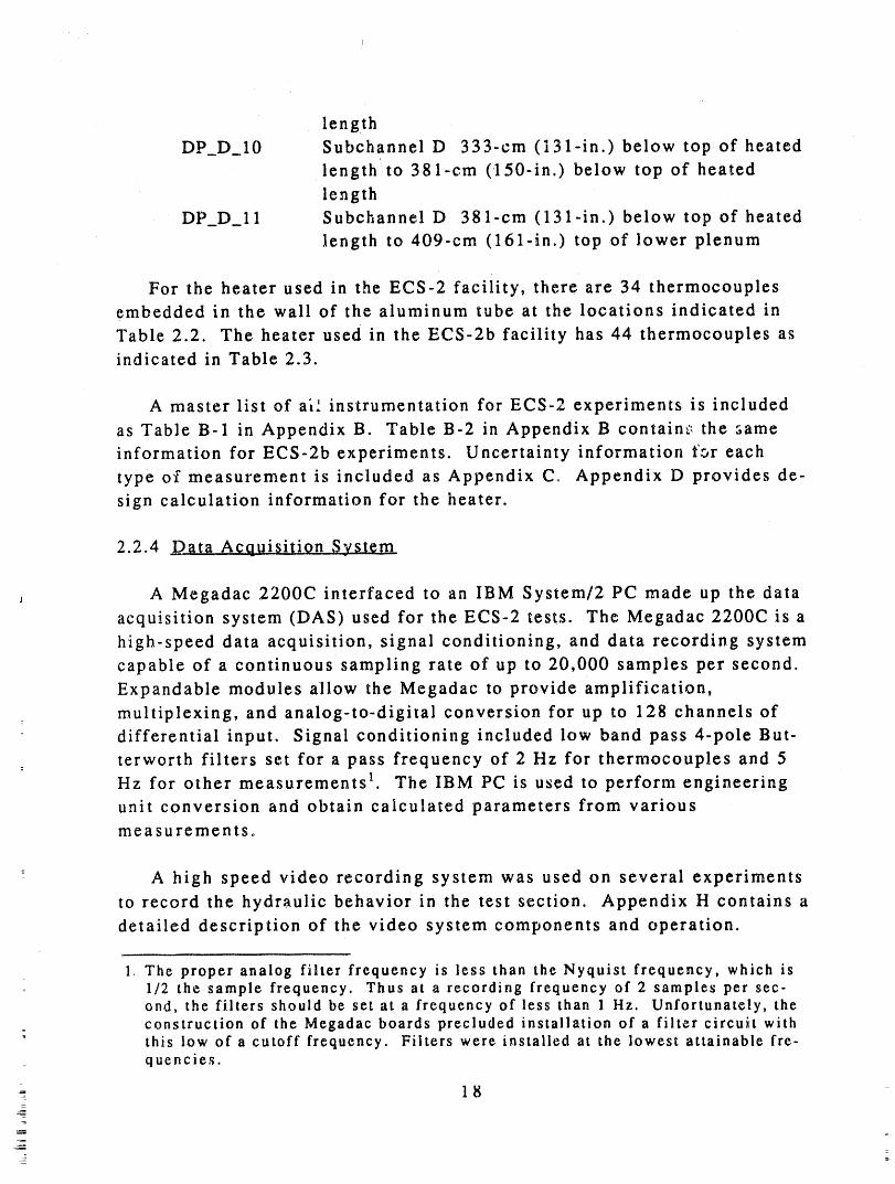
DP D 10 Subchannel D 333-cm (131-in.) below top of heated

length to 381-cm (150-in.) below top of heated

lengthDP D 11 SubchannelD 381-cm (131-in.) below top of heated

length to 409-cm (161-in.) top of lower plenum

For the heater used in the ECS-2 facility, there are 34 thermocouplesembedded in the wall of the aluminum tube at the locations indicated in

Table 2.2. The heater used in the ECS-2b facility has 44 thermocouples asindicated in Table 2.3.

A master list of ai.' instrumentation for ECS-2 experiments is included

as Table B-1 in Appendix B. Table B'2 in Appendix B contain,:' the same

information for ECS-2bexperiments. Uncertainty information for each

type of measurement is included as Appendix C. Appendix D provides de-

sign calculation information for the heater.

2.2.4 _D_ta Acquisition System

j A Megadac 2200C interfaced to an IBM System/2 PC made up the data

acquisition system (DAS) used for theECS-2 tests. The Megadac 2200Cis a

high-speed data acquisition, signal conditioning, and data recording system

capable of a continuous sampling rate of up to 20,000 samples per second.

Expandable modules allow the Megadac to provide amplification,

multiplexing, and analog,to-digital conversion for up to 128 channels ofdifferential input. Signal conditioning included low band pass 4-pole But-

terworth filters set for a pass frequency of 2 Hz for thermocouples and 5

Hz for other measurements _. The IBM PC is used to perform engineering

unit conversion and obtain calculated parameters from variousmeasurements.

-_ A high speed video recording system was used on several experiments

to record the hydraulic behavior in the test section. Appendix H contains a

detailed description of the video system components and operation.

1. The proper analog filter frequency is less than the Nyquist frequency, which is1/2 the sample frequency. Thus at a recording frequency of 2 samples per sec-ond, the filters should be set at a frequency of less than 1 Hz. Unfortunately, theconstruction of the Megadac boards precluded installation of a filter circuit with=

this low of a cutoff frequency. Filters were installed at the lowest attainable fre-quencies.

= 18

z

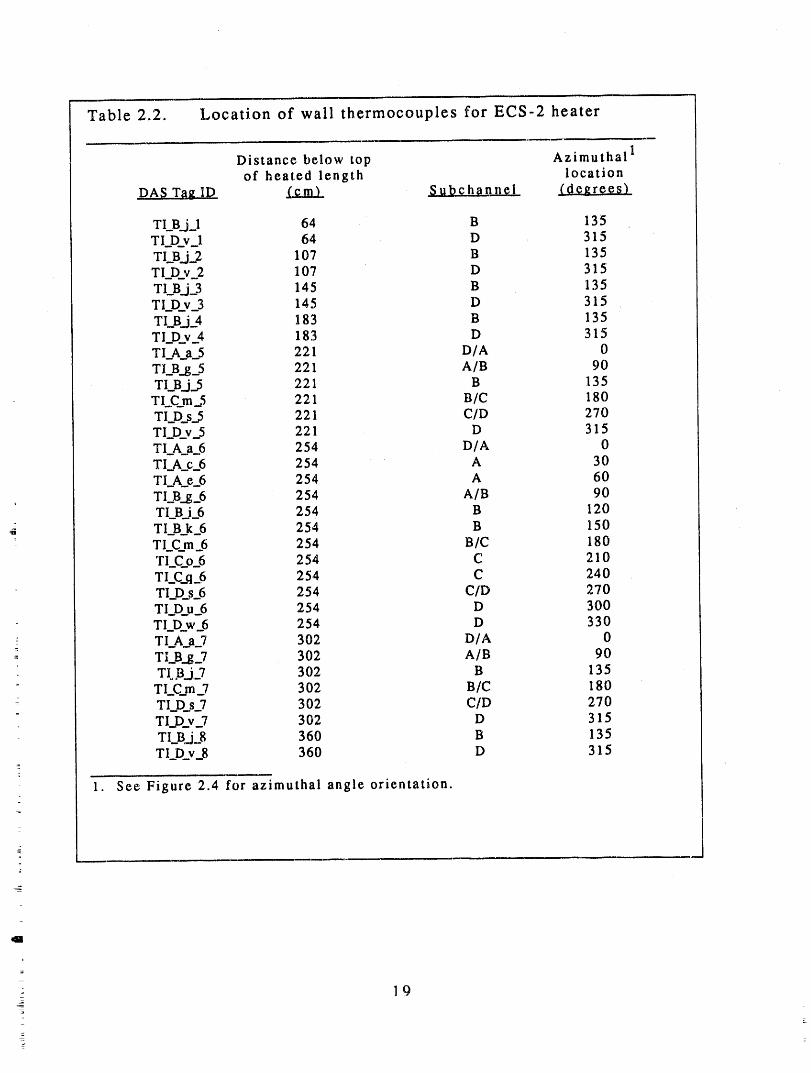
Table 2.2. Location of wall thermocouples for ECS-2 heater

Distance below top Azimuthal 1of heated length location

,DA$ Ta_ ID _ ..S..]_ hltn ngl (degrees)

TLB..j_.I 64 B 135TI_DvJ 64 D 315TLB_j..2 107 B 135TI Dv 2 107 D 315

TI_B_j3 145 B 135TI_D._v_3 145 D 315TI_B_j..4 183 B 135TI Dv 4 183 D 315

TI_A..aj 221 D/A 0TI_B_g..5 221 A/B 90TI_B.j..5 221 B 135

TI C_m_5 221 B/C 180TI_D_s..5 221 C/D 270TIDv 5 221 D 315TI A a 6 254 D/A 0TI A..c-6 254 A 30T l_A..e_6 254 A 60

, TI_B_g..6 254 A/B 90TI_Bj...6 254 B 120

_- TIBk 6 254 B 150TI_C_m__6 254 B/C 180TI_C .o_6 254 C 210TI C_q 6 254 C 240Tl_D_s-6 254 C/D 270TI_D_u_6 254 D 300TI D w 6 254 D 330

TI_A_a_7 302 D/A 0TI_B..g 7 302 A/B 90TI Bi-7 302 B 135

TI_C_m_7 302 B/C 180_

TI_D..s_7 302 C/D 270=

TI D..v..7 302 D 315TI_B.j_8 360 B 135T I_D..v..8 360 D 315

I. See Figure 2.,#forazimuthal angle orientation.

_

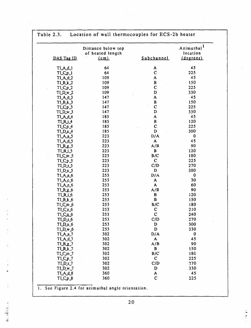
Table 2.3. Location of wall thermocouples for ECS-2b heater

Distance below top Azimuthallof heated length location

DAS Tag ID, _ $ubch_nnel (degrees)

TI_A..d_l 64 A 45TI._C..p_l 64 C 225TI_A d_2 109 A 45TI B k 2 109 B 150

TI_C..p_2 109 C 225TID w 2 109 D 330TI_A_d_3 147 A 45TI B k _ 147 B 150TI_C p..3 147 C 225TI..;Dw_3 147 D 330TI A d4 185 A 45

TLB_i..4 185 B 120TI_C p_4 185 C 225TI_D..u_4 185 D 300TI_A..a..5 223 D/A 0T I_A_d..5 223 A 45TI_B..g_5 223 A/B 90TI_B_i_5 223 B 120

TI_C_m...5 223 B/C 180TI_C_p_5 223 C 225TI._D_s_5 223 C/D 270TI D_u..5 223 D 300TI_A._a_6 253 D/A 0TI_A..c_6 253 A 30TI A..e_6 253 A 60TI_B_g_6 253 A/B 90TI B i 6 253 B 120

TI.,B_k._6 253 B 150TI Cm 6 253 B/C 180TI C.,.o_6 253 C 210

: TI_C._q_6 253 C 240TI_D._s_6 253 C/D 270T I_D..u_6 253 D 300TID w 6 253 D 330TI A a 7 302 D/A 0T I..A_d..7 302 A 45TI_B_g._7 302 A/B 90TI_B..k..7 302 B 150TI._C_m_7 302 B/C 180TI_C_p7 302 C 225TI_D._s-7 302 CID 270TI_D_w_7 302 D 330

= T I...A_d..8 360 A 45TI..C_p_8 360 C 225

_

1. See Figure 2.4 for azimuthal angle orientation.

20

3. EXPERIMENT DESCRIPTION

Procedures used to conduct wall thermal excursion experiments in t_e

ECS-2 and ECS-2b facilities and to help ensure the validity of the data base

generated during the tests are briefly described in this section: System

operational checkout and other tests conducted to verify the design,

measurement, and support systems are discussed first. Daily procedures "-

used in test setup andmeasurement calibration are then described.

Finally, the procedure t, sed to conduct actual experiments and the test ma-trices are addressed.

3.1 C__.b.h.eeckoutTests

Once the facility hardware and measurements system had beencompletely installed, numerous checkout tests were conducted to insure

that the component systems were working properly. These tests included"

(a) measurements verification

(b) system operational (SO)

(c) inner heater design and measurement systeni verification

(d) power pulse (conducted in air)

(e) power trip test

(f) single-phase liquid full heat transfer.I

, 3.1.1 _Measureme_nt Ver_ifj_

After the entire measurement and DAS had been installed, a number of

checks were conducted to guarantee proper operation of the

instrumentation and data recording system. After the DAS had been set

up with necessary calibration constants and transform fanctions, an evil-

to-end check on each individual measurement was performed. This in-

volved using known voltage insertion at the sensor location _o verify the,

proper response of the measurement signal at the DAS. Where possible, ali

measurements were checked by inserting known voltages that correspond-

ed to the endpoints of the range for which it was calibrated. This proce-

dure also allowed verification of instrument cabling, patch panel setup, and

so forth.

;. Air flow measurement outputs were verified using a technique involv-ing the use of a suction fan and soap bubbles. The system was configured"i

21

=

with a large intake pipe on the upstream side of the measurement station

being checked. An air-soap bubble mixture was drawn through the mea-surement station to produce a flowrate. With a known cross section area

of the piping, the time required for a single soap bubble to travel a knowndistance allowed calculation of the volumetric flowrate. This value was

checked against the measurement signal output to the DAS (data was not

recorded). Although crude, the methodology gave confidence in the mea-surement.

Turbine meters used to provide liquid flowrate measurement were

verified after installation using timed measurements and calibrated collec-tion devices.

Differential pressures, absolute pressures, and fluid and metal thermo-

couples in the system were verified for location and response while slowly

filiing the test section with water. Response of the measurements was

correlated with the liquid level in the test section using both hot and coldwater bottom fills.

3.1.2 _ystem Operational (SO_ Tests

The ECS-2 and ECS-2b facilities and ali supporting equipment (electrical

power, data acquisition, water supply, and so forth) were checked in an in-

tegral fashion prior tc conducting any planned experiments by conducting

System Operational tests. The objective of the SO tests was to ensure that

the overall system could function as desired. Included in the SO test were

component checks and a "dry run" for a bonafide experiment complete

with data archiving and analysis_

3.1.3 _A_irPowe.r Pulse (APP) an.0 Liquid Full (LF_ Che..g.Kg._t T_sts

Two different tests were run to verify the design details of the inner

heater. Three air power pulse tests (APP) and one liquid full (LF) power

pulse test were conducted to laelp verify the axial and azimuthal power

profile on the heater. More than 40 LF tests were conducted to examineheat transfer to single-phase liquid.

_'_P tests involved putsing the test section with a low, constant power

for approximately one minute with the test section in a dry air environ-

ment. Such a heatup in air was expected to result in a nearly adiabaticc

22

heatup rate of the test section. Rise rates for each wall thermocouple could

then be related to the local power generation rate for comparison to ex-

pected values and to investigate evidence of azimuthal variation. Details ofthe APP tests and conclusions reached are documented in Appendix E of

Anderson [11]. APP test results verified that the axial pl_wer profile was

per design specifications and that there were no significant azimuthal

• power gradients.

One liquid full power pulse test and one air power trip test were con-

: ducted to help resolve questions regarding the potential effects of electri-

cal and magnetic fields (induced by the power supply) on the aluminumwall thermocouple readings. Results of these experiments showed that

there was no influence of electrical and magnetic fields on the aluminum

wall thermocouple readings.

Liquid full tests were run to examine the axial variation in heat trans-

fer to single-phase liquid. These tests were run by setting the standpipe at

a level above the top of the heated length to ensure only liquid flowexisted in the flow channel. Heat transfer coefficients were then computed

from the data and compared with expected values to establish confidence

in the data. Details of several of the LF tests and results from the analysis

of LF test dataare contained in Appendix F of Anderson [11]. Additional

information pertaining to the results of the LF tests will be published in an

addendum to Anderson's report._

3.2 ._.9,0tin_ Data lntc_grity Ch¢,cks

To ensure the integrity of the data produced in the ECS-2 facility, cer-

o tain procedures ,,ere routinely performed (weekly, daily, or before every_

" test) as required.z

DAS balance and calibration were electronically checked daily. Even

though the DAS electronics were very stable, electronic balance and two_

point calibration on the cards in the DAS were performed weekly, or

following instrument changeout or measurement channel patch changes.

i Differential pressure transducers were checked daily. The cells werevalved out of the system, the sense lines were backfilled, and the

instruments were checked for any abnormal zero offsets (offsets were cor-_

rected if found), and then valved back into the system.

- 23=

_

Pretest and posttest scans of ali measurements were conducted for

each test. Known, steady-state thermal conditions were established in the

test section, Review of this information helped to identify any problemswith measurement and electronics consistency. The fluid temperature

reading from a calibrated glass thermometer, installed at the inlet to the

test section, was compared with the inlet fluid thermocouples to ensure

measurement consistency.

Daily, barometric pressure readings, obtained from the INEL Standards

and Calibration Laboratory, were recorded in the test operations log book.

Water pH measurement results were also recorded daily irl the test opera-

tions log book (The test operations log book for the ECS-2 experiments con-

sists of three volumes. Copies of these volumes are located in the INEL

Technical Library and have identification numbers INEL-NBU-2205, INEL-

NBU-2206,and INEL-NBU-2207).

3.3 Experimental Pr o.¢eclure

Most thermal excursior, experiments conducted in the ECS-2 and ECS-

2b facilities were conducted using the same procedure. For any given ex-

periment, the sequence of events was as follows"

Before initia_ign of powc_r to the heater

• Set test section standpipe to desired value• Initiate inlet flow and set to desired value

• Start the heated water makeup system and adjust the fluid

temperature to the desired value

• Start DAS (in monitor mode)

• Verify systems operating.

Test Initiation

• Initiate DAS record 2 minutes prior to application of power

• Set Inconel test section power to approximately 20 kW and

maintain sufficiently long to achieve thermal equilibrium

• Increase test section power by an increment specified by the

test engineer followed by a 2-5 minute soak period

• Record video data per the direction of the test engineer

• Increase test section power by an increment of approximately

20 kW (discretion of the test engineer) followed by a 2-5

24

minute soak period. If thermal excursion does not occur dur-

ing the power increase, maintain the power setting for ap-

proximately 5 minutes to allow system to soak and come to

thermal equilibrium

• Continue increasing the test section power in steps followed

by a 5 minute soak period until thermal excursion occurs or

the test section is at maximum power

• When the test criteria are met (sustained thermal excursion),

terminate test section power (normally done automatically by

a power trip circuit that monitored specified metal

temperatures)• Terminate DA$ record.

P0sttest ACtivities• Archive recorded data

• Conduct engineering units calculations and prepare Quick

Look plots

° Cont, uct posttest facility check.

Experiments in the flow coastdown series (ECS-2FC) deviated somewhat

from this procedure. For the flow coastdowns, the test section power was

held constant while the inlet flow was decreased in discrete steps from the

initial value. In th_' ECS-2cE experiments, permanent data recording was

not initiated until the test section was near (within approximately 10 kW)

thermal excursion, power increases were limited to 3 kW, and the soak

time at any given power was at least 6 minutes.

The goal for tests in the thermal excursion program was to establish

and measure the conditions (test section flowrate, power, inlet fluid

temperature, and lower plenum pressure) leading to sustained thermal

excursion at any position along the axial length of the heater. The excur-sion criteria and hence test termination criteria were defined based on

maximum aluminum wall temperature. For the majority of the INEL ex-

- periments, this maximum temperature was 620 K. On some of the later

experiments, the temperature criterion was decreased to 520 K to be con-

sistent with similar experiments conducted at SRS. Data repeatability and_

the impact of the different excursion cri:eria are discussed in Appendix F.

In addition to the maximum wall criteria, an ancillary test section

power limit criterion was implemented to provide heater protection during

25

nllll ..... ,,_l, rq,, iii ,r _,..... rl _'l_ ,'?l Plllql' _pl' _,_,, ,_ ..... vi I1m li q_",_ln,'_l[llr'

the thermal excursion experiments. Equipment design considerations

limited the maximum heater power to less than 175 kW. Most

experiments, however, were successfully completed at heater powers lessthan 150 kW.

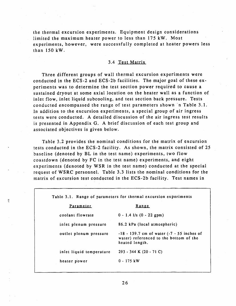
3,4 Test Matrix

Three different groups of wall thermal excursion experiments were

conducted in the ECS-2 andECS-2b facilities. The major goal of these ex-

periments was to determine the test section power required to cause a

sustained dryout at some axial location on the heater wall as a function of

inlet flow, inlet liquid subcooling, and test section back pressure. Tests

conducted encompassed the range of test parameters shown n Table 3.1.

In addition to the excursion experiments, a special group of air ingresstests were conducted. A detailed discussion of the air ingress test results

is presented in Appendix G, A brief discussion of each test group and

associated objectives is given below.

Table 3.2 provides the nominal conditions for the matrix of excursion

• tests conducted in the ECS-2 facility. As shown, the matrix consisted of 25

baseline (denoted by BL in the test name) experiments, two flow

coastdown (denoted by FC in the test name) experiments, and eight

experiments (denoted by WSR in the test name) conducted at the special

request of WSRC personnel. Table 3.3 lists the nominal conditions for the

matrix of excursion test conducted in the ECS-2b facility. Test names in

Table 3.1. Range of parameters for thermal excursion experiments

Parameter Range

coolant flowrate 0 - 1.4 l/s (0 - 22 gpm)

inlet plenum pressure 86.2 kPa (local atmospheric)

outlet plenum pressure -18 - 139.7 cm of water (-7 - 55 inches ofwater) referenced to the bottom of theheated length.

inlet liquid temperature 293 - 344 K (20 - 71 C)

heater power 0 - 175 kW

J ......

z

26

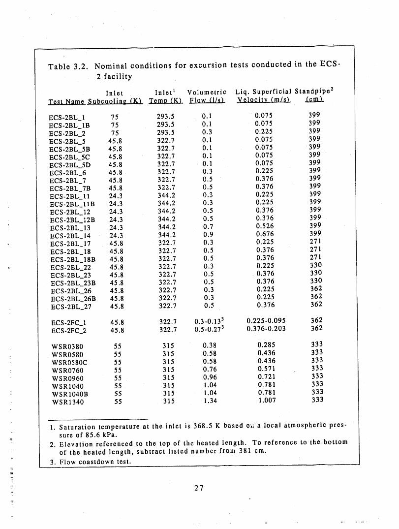
Table 3.2. Nominal conditions for excursion tests conducted in the ECS-

2 facility

Inlet Inlet 1 Volumetric Liq. Superficial Standpipe 2Subcoolin_ CK_ Temp (K) .E.Lo._LL[LLL Velocity (m/s) ,£g,tIl.L

ECS-2BL_I 75 293.5 0.1 0,075 399ECS-2BL_IB 75 293.5 0.1 0,075 399ECS-2BL_2 75 293.5 0,3 0.225 399ECS-2BL_5 45.8 322.7 0.1 0,075 399ECS-2BL_5B 45.8 322.7 0.1 0,075 399ECS-2BL 5C 45.8 322.7 0.1 0.075 399ECS-2BL 5D 45.8 322.7 0.1 0.075 399EC S-2 BL_6 45.8 322.7 0.3 0.225 399ECS-2BL 7 45.8 322,7 0.5 0.376 399ECS-2BL 7B 45.8 322.7 0.5 0.376 399EC S-2BL, 11 24.3 344.2 0.3 0.225 399ECS-2BL_I 1B 24.3 344.2 0.3 0.225 399ECS-2BL 12 24.3 344.2 0.5 0.376 399ECS-2BL 12B 24.3 344.2 0.5 0.376 399ECS-2BL 13 24.3 344.2 0.7 0.526 399ECS-2BL 14 24.3 344,2 0.9 0.676 399ECS-2BL 17 45.8 322.7 0'3 0.225 271ECS-2BL_18 45.8 322.7 0.5 0.376 271ECS-2BL 18B 45.8 322.7 0.5 0.376 271ECS-2BL_22 45.8 322.7 0.3 0.225 330ECS-2BL_23 45.8 322,7 0.5 0.376 330ECS-2BL_23B 45,8 322.7 0.5 0.376 330ECS-2BL_26 45.8 322.7 0.3 0.225 362ECS-2BL_26B 45.8 322.7 0.3 0.225 362ECS-2BL_27 45.8 322.7 0.5 0.376 362

ECS-2FC_I 45,8 322,7 0.3-0,133 0,225-0,095 362ECS-2FC_2 45.8 322.7 0.5 -0_273 0,376-0.203 362

WSR0380 55 315 0,38 0,285 333WSR0580 55 315 0.58 0.436 333WSR0580C 55 315 0.58 0.436 333WSR0760 55 315 0.76 0.571 333WSR0960 55 315 0.96 0.721 333WSR 1040 55 315 1.04 0.781 333WSR 1040B 55 315 1,04 0.781 333WSR1340 55 315 1.34 1.007 333

1. Saturation temperature at the inlet is 368.5 K based o_a a local atmospheric pres-sure of 85.6 kPa.

2. Elevation referenced to the top of the heated length. To reference tothe bottomof the heated length, subtract listed number from 381 cm.

3. Flow coastdown test.

: 27

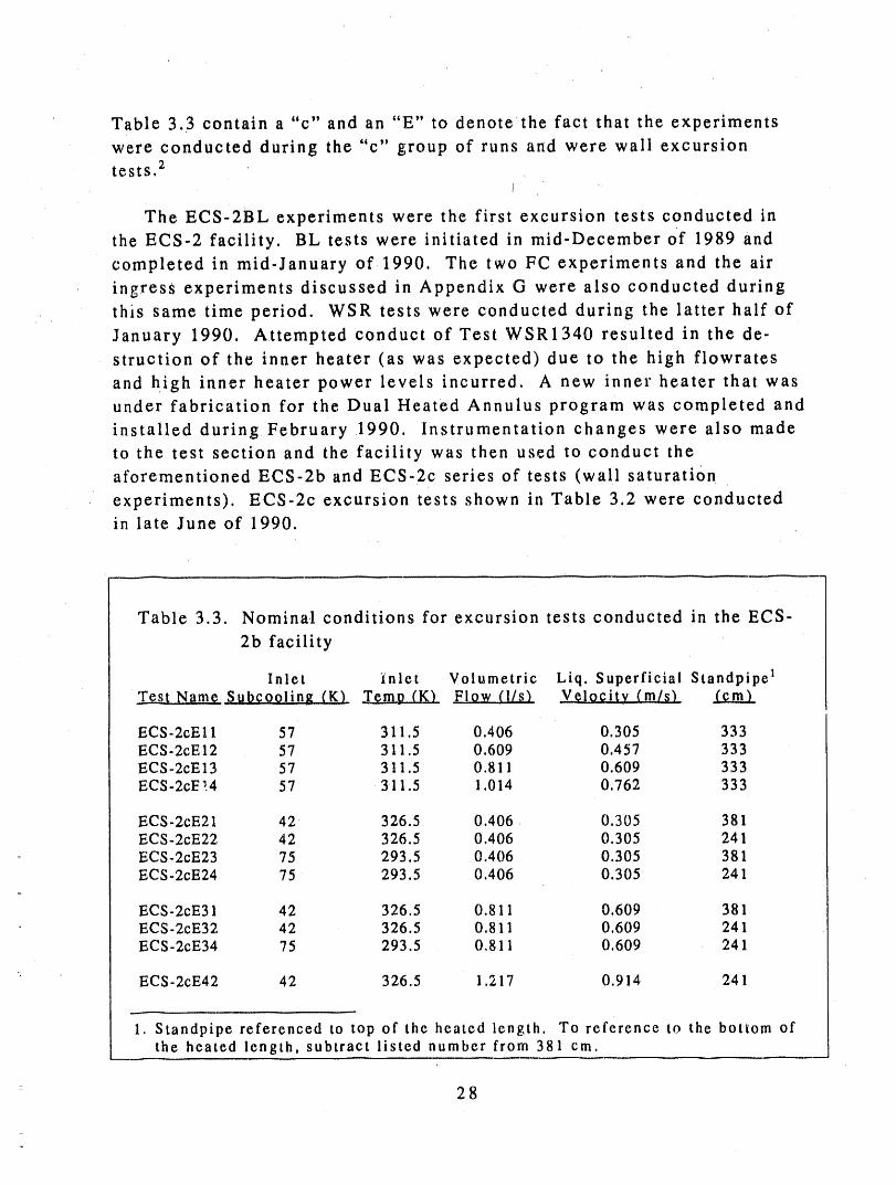
Table 3.3 contain a "c" and an "E" to denote the fact that the experiments

were conducted during the "c" group Of runs and were wall excursion2tests,

The ECS-2BL experiments were the first excursion tests conducted in

the ECS-2 facility. BL tests were initiated in mid-December of 1989 and

completed in mid-January of 1990, The two FC experiments and the air

ingresS experiments discussed in Appendix G were also conducted during

this same time period. WSR tests were conducted during the latter half of

January 1990, Attempted conduct of Test WSR1340 resulted in the de-struction of the inner heater (as was expected) due to the high flowrates

and high inner heater power levels incurred. A new inner heater that wasunder fabrication for the Dual Heated Annulus program was completed and

installed during February 1990, Instrumentation changes were also made

to the test section and the facility was then used to conduct theaforementioned ECS-2b and ECS-2c series of tests (wall saturation

experiments). ECS-2c excursion tests shown in Table 3,2 were conductedin late June of 1990,

Table 3.3. Nominal conditions for excursion tests conducted in the ECS-

2b facility

Inlet inlet Volumetric Liq. Superficial Standpipe 1T_st Namg .Subcooling (K_ ..T_g._p._.(__ Flow (l/s_ V eLo_iLy (m/s_ .(.._.m__L

ECS-2cE11 57 311.5 0.406 0.305 333ECS-2cE 12 57 311.5 0.609 0.457 333ECS-2cE13 57 311.5 0.811 0.609 333ECS-2cE _.4 57 311.5 1.014 0.762 333

ECS-2cE21 42 326.5 0.406 0.305 381ECS-2cE22 42 326.5 0.406 0.305 241ECS-2cE23 75 293.5 0.406 0.305 381ECS-2cE24 75 293.5 0.406 0.305 241

ECS-2cE31 42 326.5 0.811 0.609 381ECS-2cE32 42 326.5 0,811 0.609 241ECS-2cE34 75 293.5 0.811 0.609 241

ECS-2cE42 42 326.5 1.217 0.914 241

1. Standpipe referenced to top of the heated length. To reference to the bottom ofthe heated length, subtract listed number from 381 cre.

= 28

Ali of the excursion tests conducted were specified with input from WSRC

personnel and reflect boundary conditions expected tc represent reactorconditions or those required to duplicate as closely as possible experiments

previously conducted at the SRS Heat Transfer Laboratory. For example,

the BL series was designed to provide information on the effects of a range

of inlet fluid temperature, inlet flowrate, and facility back pressure. The

two FC tests provided information on the effects of transient flow _;ondi-

tions with test section inlet temperature, flowrate, back pressure, and

power held constant. Specifications for the WSR tests reflect the desire to

duplicate flowrate boundary conditions for experiments that had been con-

ducted at the SRS Heat Transfer Laboratory_ Inlet flowrate was the prima-

ry variable and neither the inlet fluid temperature or the back pressure

were altered during the WSR tests. Objectives of the ECS-2cE experiments

were twofold. Fluid temperature and back pressure boundary conditionsused are the same values used in the wall saturation tests and reflect the

current best estimate values for reactor conditions. 3 Also, the facility

hardware was somewhat different relative to the ECS-2 system since a

new inner heater was installed and instrumentation changes were effected.

ECS-2cE experimental data therefore offer an opportunity to check for any

systematic effects due to system hardware.

2. The m_.iority of the ECS-2b program centered around investigation of wall satura-tion criteria. Two different groups of runs, the"b" and"c" series, were conductedto examine conditions satisfying the, wall saturation criteria.

° 3. Improvements in computer code predictions and changes in assumptions aboutthe LBLOCA since the BL tests were conducted led to small changes in the best esti-mate boundary conditions.

29

4. RESULTS

Excursion test results are presented in this section. An overview of a

typical test will be given first to illustrate test conduct, provide a flavor for

the nature of the time series data produced, and explain the data

presentation format. Characteristics of the wall temperatures, pressuresand differential pressures, fluid temperatures, and air entrainment are

discussed. A general description of the factors influencing the wall tem-

perature excursion is then provided. Finally, all the data recorded is sum-

marized and _-_sented in terms of the R factor (power at the limits criteria

of interest divided by the power required to saturate the fluid at the outlet

of the test section) Results from both the INEL experiments and the SRS

experiments are included. Appendix I contains a list of the measurements

that were failed or determined to be questionable for each experiment.

Appendix J contains tables of data averages for the power step before ex-

cursion and the power step at which excursion occurred for ali of the INEL

experiments.

4.1 _Typical Test Results

Data from Tests ECS-2BL_5 are presented to illustrate results from a

typical thermal excursion experiment. This particular experiment wasconducted on several different occasions and is the basis for the data re-

peatability discussion in AppendixF. ECS-2BL 5 was conducted from nom-

inal conditions of 322.7 K inlet fluid temperature (45.8 K subcooling), an

inlet flowrate of 0.1 1/s (superficial velocity of 0.075 m/s), and with an

outlet standpipe setting of 43 cm referenced to the bottom of the lower

plenum (399 cm relative to the top of the heated length or-18 cm relative

to the bottom of the heated length). This test was typical of low flow tests

with multiple dryout-rewet cycles before a sustained dryout and thermal

excursion that occurred at a saturation ratio (R factor) significantly larger

than unity.

ECS-2BL_5 was conducted using the procedure discussed in Section 3.3.

After the desired inlet fluid temperature and flowrate were established,

data recording was initiated, the heater power was increased to 10 kW and

held for 5 minutes while the system came to thermal equilibrium. Power

was then increased by roughly 5 kW increments with 1-2 minute hold pe-riods over the next 35 minutes until thermal excursion occurred. This ex-

30_

=

since ECS-2BL_5 was one of the first excursion experiments conducted and

expectations regarding the power at which dryout would occur were not

yet clear. Test results indicated that the test section underwent a sus-

tained dryout about 35 minutes after power was initiated at a power of53.5 kW.

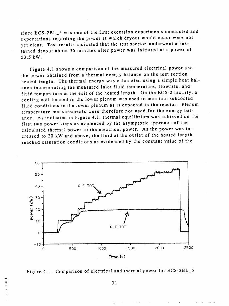
Figure 4.1 shows a comparison of the measured electrical power and

the power obtained from a thermal energy balance on the test section

heated length. The thermal energy was calculated using a simple heat bal-

ance incorporating the measured inlet fluid temperature, flowrate, and

fluid temperature at the exit of the heated length. On the ECS-2 facility, acooling coil located in the lower plenum was used to maintain subcooled

fluid conditions in the lower plenum as is expected in the reactor. Plenum

temperature measurements were therefore not used for the energy bal-

ance. As indicated in F_.gure 4.1, thermal equilibrium was achieved on the

first two power steps as evidenced by the asymptotic approach of the

calculated thermal power to the electrical power. As the power was in-creased to 20 kW and above, the fluid at the outlet of the heated length

reached saturation conditions as evidenced by the constant value of the

60 .................

50

40 " "

20

1_, 10

(3

-I0 I ....... i :" ' '"-- I ..... " I " --"' lr I _ .... II

0 soo 1000 1500 2000 2500

Time (s)

Figure 4.1. Comparison of electrical and thermal power for ECS-2BL__5

31

.

thermal power.

A cursory examination of the data in Figure 4.1 indicates that when

the excursion criteria were met, the power input to the test section was

nearly three times the amount of power required to saturate the fluid at_he outlet of the heated length (53.5 kW relative to 20 kW required to sat-

urate the outlet test section).

4.1.1 Wall.Temperatures

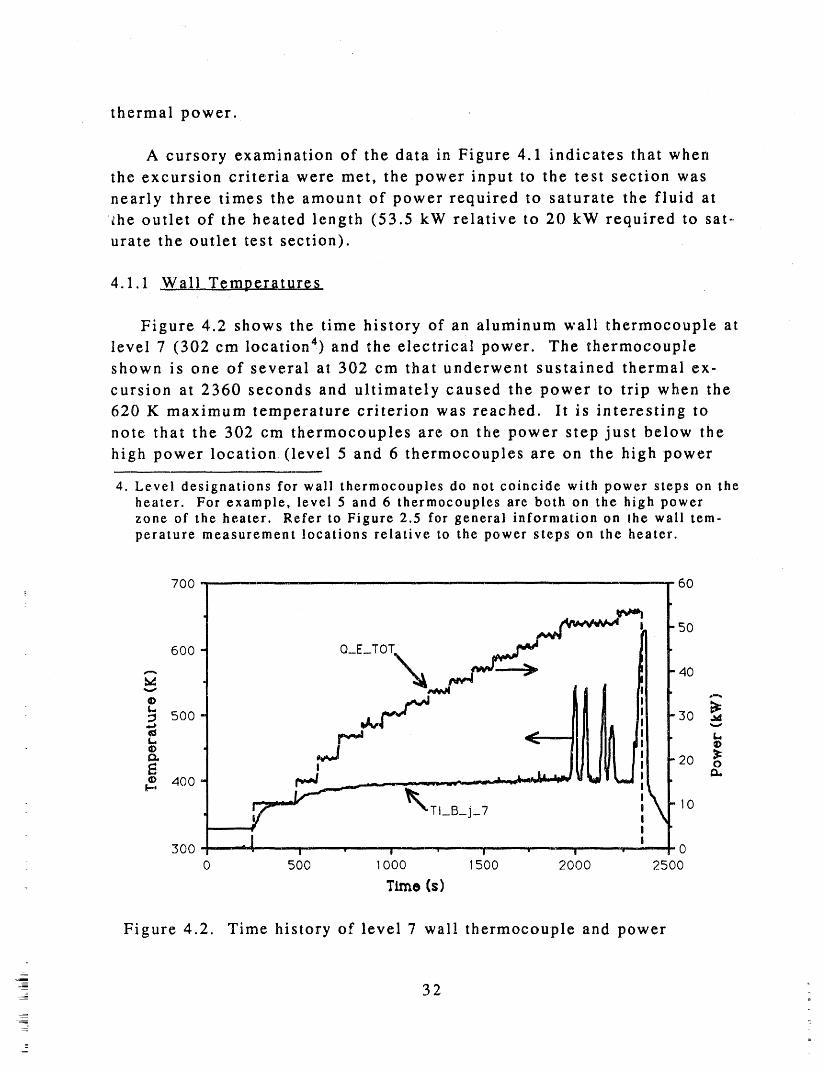
Figure 4.2 shows the time history of an aluminum wall thermocouple atlevel 7 (302 cm location 4) and the electrical power. The thermocoupleshown is one of several at 302 cm that underwent sustained thermal ex-

cursion at 2360 seconds and ultimately caused the power to trip when the

620 K maximum temperature criterion was reached, lt is interesting to

note that the 302 cm thermocouples are on the power step just below the

high power location (level 5 and 6 thermocouples are on the high power

4. Level designations for wall thermocouples do not coincide with power steps on theheater. For example, level 5 and 6 thermocouples are both on the high powerzone of the heater. Refer to Figure 2.5 for general information on the wall tem-perature measurement locations relative to the power steps on the heater.

7OO ' 6O

:

L,500 30

- J_ 20

4oo ---- i10

TI_B_j_7 i, . |

.I I300 - •.........., • ' , '" _ ', " .--"-- 0

0 500 1000 1500 2000 2500

Time (s)

Figure 4.2. Time history of level 7 wall thermocouple and power

-I 32

=

zone). As discussed in Appendix F, sustained dryout did not always occur

at level 7 and initiate the trip. Occasionally, level 6 thermocouples met the

criteria before those at level 7 (see Figure 2.5).

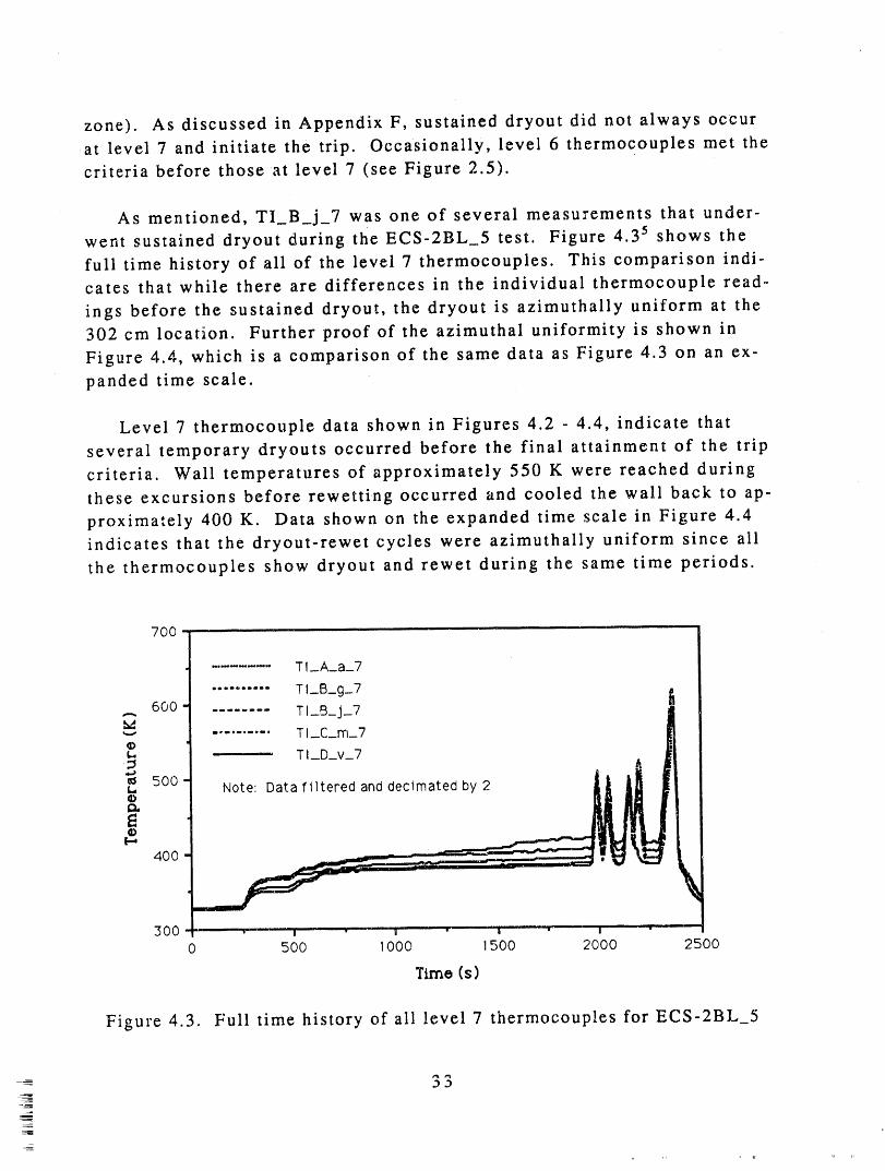
As mentioned, TI_B_j_7 was one of several measurements that under-

went sustained dryout during the ECS-2BL_5 test. Figure 4.35 shows the

full time history of all of the level 7 thermocouples. This comparison indi-

cates that while there are differences in the individual thermocouple read-

ings before the sustained dryout, the dryout is azimuthally uniform at the

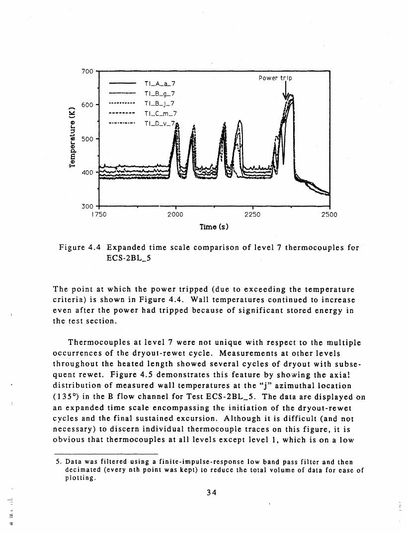
302 cm location. Further proof of the azimuthal uniformity is shown in

Figure 4.4, which is a comparison of the same data as Figure 4.3 on an ex-

panded time scale.

Level 7 thermocouple data shown in Figures 4.2 - 4.4, indicate that

several temporary dryouts occurred before the final attainment of the trip

criteria, Wall temperatures of approximately 550 K were reached during

these excursions before rewetting occurred and cooled the wall back to ap-

proximately 400 K. Data shown on the expanded time scale in Figure 4.4

indicates that the dryout-rewet cycles were azimuthally uniform since ali

the thermocouples show dryout and rewet during the same time periods.

700 TM

......... T I_A__a_7

.......... T I_B_g_7 a

600 TI_B_j_7 II.......... T l_C_rn_7

:_ .._ i_i__. T I_D_v_7

500 Note: Datafilte

400 _ , ,_

300 • 'l'l' ' _ u .... • i =T" I "

0 500 I000 1500 2000 21500

Timo (s)

Figure 4.3. Full time history of all level7 thermocouples forECS-2BL_5

33

700 "Power trip

T I_A_a__7

............ T I_B_g_7

600 .......... TI_B_j_7

_ ........ T I_C_m_7

I_ "'" ....... TI_D_V_7_ ,_ _

AIII4OO

300 __1750 2000 2250 2500

Time (s)

Figure 4.4 Expanded time scale comparison of level 7 thermocouples forECS-2BL_5

The point at which the power tripped (due to exceeding the temperaturecriteria) is shown in Figure 4.4. Wall temperatures continued to increase

even after the power had tripped because of significant stored energy inthe test section.

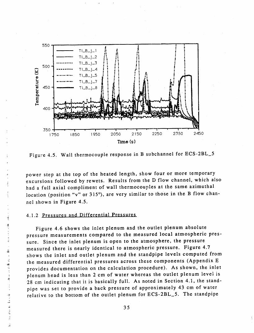
Thermocouples at level 7 were not unique with respect to the multipleoccurrences of the dryout-rewet cycle. Measurements at other levels

throughout the heated length showed several cycles of dryout with subse-

quent rewet. Figure 4.5 demonstrates this feature by showing the axia!

distribution of measured wall temperatures at the "j" azimuthal location

(135 °) in theB flow channel for Test ECS-2BL_5. The data are displayed on

an expanded time scale encompassing the initiation of the dryout-rewet

cycles and the final sustained excursion. Although it is difficult (and not

necessary) to discern individual thermocouple traces on this figure, it is

obvious that thermocouples at ali levels except level 1, which is on a low

5. Data was filtered using a finite-impulse-response low band pass filter and thendecimated (every nth point was kept) to reduce the total volume of data for ease ofplotting.

34

-

550 ..... , • -

TI_B_j_I 4 ii i |" i! 'i ;

............ i_ .i' in ' i

- . TI_B_j_.2 ' " ,; -. # •500 TI_B._j_3 i; i i I,'I .1 !,A TI_B_j_.4 i .,i tiI # lI,d , m i • i i i

........... TI B ' 5 ' ! i : , f, ; i--J- _' _ i i : 'i !

,t .......... T,Bj_7I ;' ,, -;,;4') i450 - - I ! o ; ; .._d

I li _' i I i III i _ I i I• I1' . P • ,,wl _! _- I I '

3501750 1850 1950 2050 2150 2250 2350 2450

- TimeCs)

: FiguT"e 4.5. Wall thermocouple response in B subchannel for ECS-2BL_5

power step at the top of the heated length, show four or more temporary. excursions followed byrewets. Results from the D flow channel, which also

had a full axial compliment of wall thermocouples at the same azimuthal=

location (position "v" or 315°), are very similar to those in the B flow chan-

nel shown in Figure 4.5.z

4.1.2 Pressures anal Differential Pressure8=

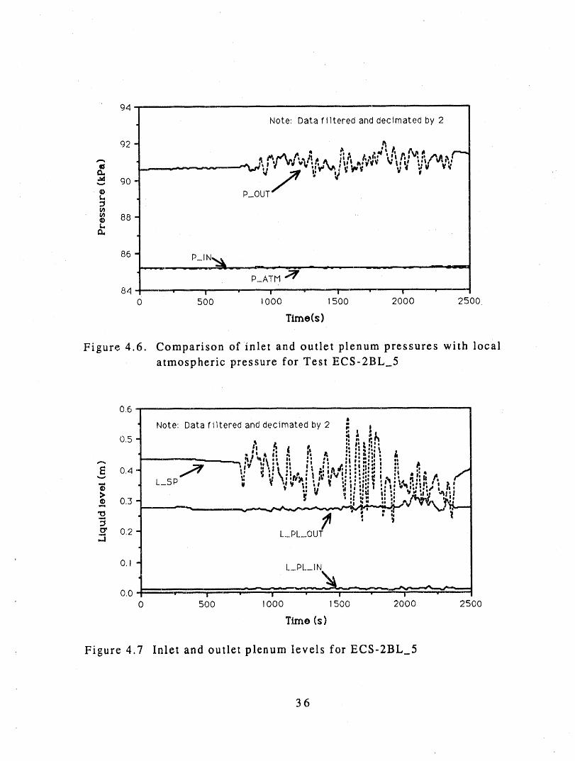
Figure 4.6 shows the inlet plenum and the outlet plenum absolutepressure measurements compared to the measured local atmospheric pres-sure. Since the inlet plenum is open to the atmosphere, the pressure

= measured there is nearly identical to atmospheric pressure. Figure 4.7shows the inlet and outlet plenum and the standpipe levels computed fromthe measured differential pressures across these components (Appendix Eprovides documentation on the calculation procedure). As shown, the inletplenum head is less than 2 cm of water whereas the outlet plenum level is28 cna indicating that it is basically full. As noted in Section 4.1, the stand-

: pipe was set to provide a back pressure of approximately 43 cm of waterrelative to the bottom of the outlet plenum for'ECS-2BL_5. The standpipe

-

35

94 .........................

Note: Data filtered and decimated by 2

92

I: lr Iii¥ _el |t, ho 'l'_' _ I I" "_I_ v

N 90P OUT"

1/)884)

I.

86P_l N_,_ _ ;_ .........

P_ATM _

84 • I ......_I i _11 I I I - ! .... !

0 500 1000 1500 2000 2500L

Time(s)

Figure 4,6. Comparison of inlet and outlet plenum pressures with localatmospheric pressure for Test ECS-2BL_5

0,6 •

1

Note: Data filtered and decimated by 2 ?. a

I I I q

, ----!.i,,.._ eG I,_ al II :I .oo .oII_' le i I I Ii I1_ il Ii _ "0,4 ,. ....... , i,--,

I I I I I I I •I____r V } _I y I I II I i | I I .' |. _liIl.I_ a .|1

11 I dills - Iii i l

--_) 0,3 ,, _ v....."_ _, . ,,

_ 0,2 L_PL._OUT,-1

0,1 L_PL_IN\,

i i L- i_ _..i_,_'*IIIl_

0.0 • , • , .....0 500 1000 1500 2000 2500

Time (s)

: Figure 4.7 Inlet and outlet plenum levels for ECS-2BL_5

36

level shown irl Figure 4.7 verifies the level setting.

As expected, pressure and differential pressure measurements in the

test section showed substantial oscillation during the experiment, particu-

larly after saturation conditions were achieved at the outlet of the heated

length. As will be illustrated in the next section, the liquid at the outlet of

the heated length reached saturation conditions just after 750 seconds.

Substantial vapor generation and holdup ensued resulting in a churn-tur-bulent flow regime in the test section. The unsteady nature of the local

flows caused the fluctuations noted in the measurements. Although not

evident on ECS-2BL_5, the holdup in the test section for many experiments

was sufficient to cause the inlet plenum level to increase significantly.

For Test ECS-2BL_5, an absolute pressure measurement was located in

each subchannel at the beginning of the heated length. These measure-

ments suffered from zero offsets during this test and the data are not pre--- sented here. Instead, data from Test ECS-2BL_5B (conditions on BL_5B are

identical to those on BL 5 as discussed in Appendix F) are presented in

Figure 4.8. Data from these two tests are directly comparable until about

1600 seconds. In order to prevent undue clutter on the figure, only the

data from the B and D subchannels is shown since the response of each

measurement is very similar. The pressure behavior is consistent with the

wall temperature measurements presented in Section 4.1.1 in that there is=

azimuthal uniformity in the oscillations even though at any given time,

there are slight differences in magnitude, lt should be noted that the

pressure data from Test ECS-2BL_5 showed the same basic response with

the exception that due to an electronics problem, the magnitudes were 30kPa above atmospheric pressure.

From the data shown in Figure 4.8, ,t is apparent that the pressure at

the inlet to the heated length increased slightly (1-2 kPa) when the test

section outlet became saturated at 750 seconds. Although the increase is

-_ minor, it is consistent with visual observations during the experiment that

suggested water accumulation (void fraction was decreasing slightly) in the

unheated part of the test section between the bottom of the inlet plenum

and the entrance to the heated length. This observation is consistent with

the expected increase in two-phase pressure drop through "he test section

in light of local flooding noted along the heated length.

_

37=

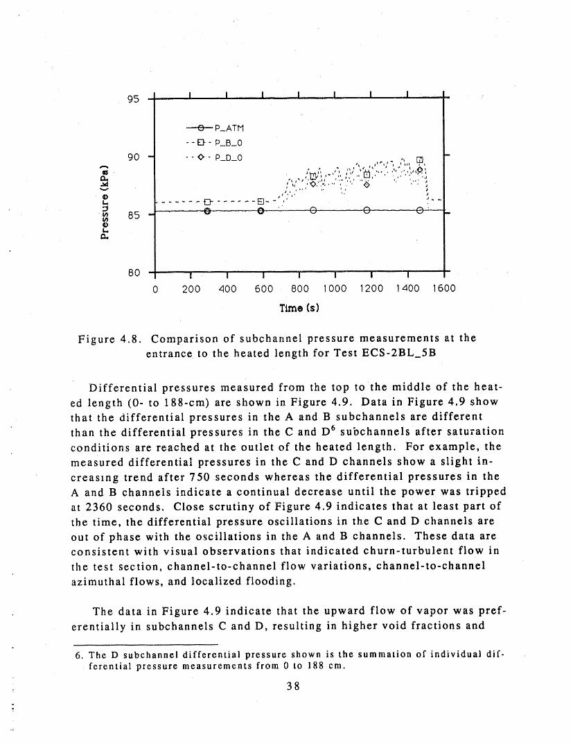
95 .... I I I I , I I I :

80 U "'1 "'1 I I I I

0 200 400 600 800 1000 1200 1400 1600

Time (s)

Figure 4.8. Comparison of subchannel pressure measurements at the

entrance to the heated length for Test ECS-2BL_5B

Differential pressures measured from the top tothe middle of the heat-

ed length (0- to 188-cm) are shown in Figure 4.9. Data in Figure 4.9 showthat the differential pressures in the A and B subchannels are different

than the differential pressures in the C and D 6 subchannels after saturationconditions are reached at the outlet of the heated length. For example, the

measured differential pressures in the C and D channels show a slight in-

creasxng trend after 750 seconds whereas the differential pressures in theA and B channels indicate a continual decrease until the power was tripped

at 2360 seconds. Close scrutiny of Figure 4.9 indicates that at least part of

the time, the differential pressure oscillations in the C and D channels are

out of phase with the oscillations in the A and B channels. These data areconsistent with visual observations that indicated churn-turbulent flow in

the test section, channel-to-channel flow variations, channel-to-channel

azimuthal flows, and localized flooding.

The data in Figure 4.9 indicate that the upward flow of vapor was pref-

erentially in subchannels C and D, resulting in higher void fractions and

6. "['he D subchannel differential pressure shown is the summation of individual dif-ferential pressure measurements from 0 to 188 cm.

38

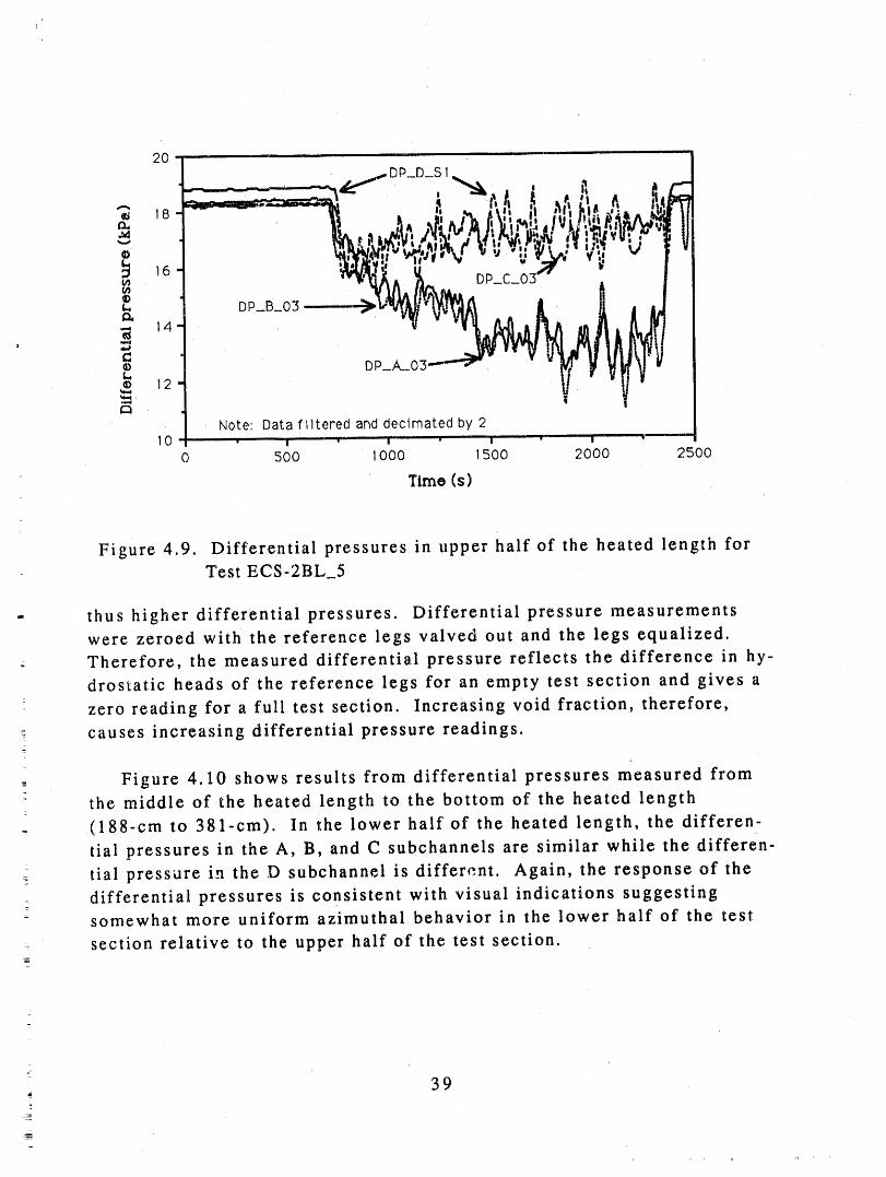
0 , ,,i i ,, , ,,, ,.,. .....

J. DP_D_S I

,s sll | IIIi la. ,. 1

;Y,.TY_,,,: e, . "v v "--li_' v!;

_ _. DP_C_03 A

Note', Data filtered and decimated by 210 ' • , • I • ' , '_'" , • "--

0 500 1000 1500 2000 2500

Time (s)

Figure 4.9. Differential pressures in upper half of the heated length forTest ECS-2BL_5

thus higher differential pressures. Differential pressure measurements

were zeroed with the reference legs valved out and the legs equalized.Therefore, the measured differential pressure reflects the difference in hy-

drostatic heads of the reference legs for an empty test section and gives a

zero reading for a full test section. Increasing void fraction, therefore,

- causes increasing differential pressure readings.

Figure 4.10 shows results from differential pressures measured from-

the middle of the heated length to the bottom of the heated length

(188-cm to 381-cm). In the lower half of the heated length, the differen-

tial pressures in the A, B, and C subchannels are similar while the differen-

tial pressure in the D subchannel is different. Again, the response of the

differential pressures is consistent with visual indications suggestingsomewhat more uniform azimuthal behavior in the lower half of the test

section relative to the upper half of the test section.

39

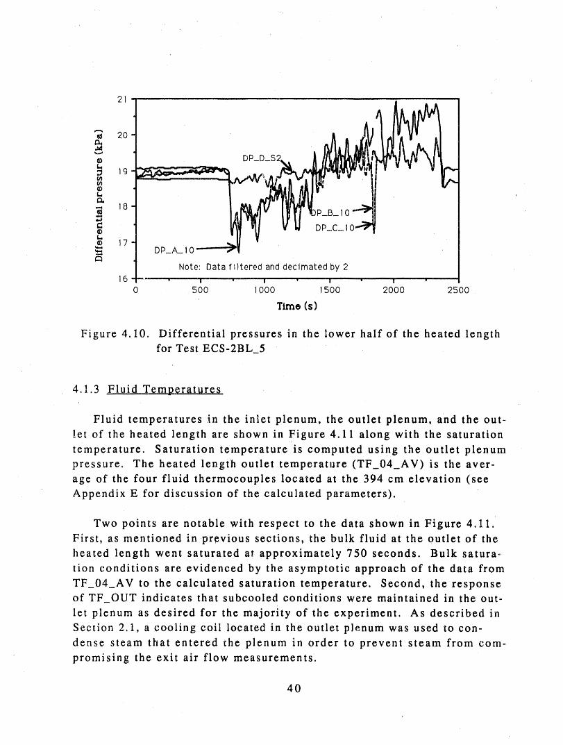
1 i i i i i u

"_ 20

- _ ,,- ,DP_C_IO_L,

"'_, i 7 DP_A__I 0

Note: Data filtered and decimated by 216 ....... • .... I "" • I • I ' • I '

0 500 1000 1500 2000 2500I

Time (s)

Figure 4.10. Differential pressures in the lower half of the heated lengthfor Test ECS-2BL_5

4.1.3 Fluid Temperatures

Fluid temperatures ,in the inlet plenum, the outlet plenum, and the out-

let of the heated length are shown in Figure 4.11 along with the saturation

temperature. Saturation temperature is computed using the outlet plenumpressure. The heated length outlet temperature (TF_04_AV) is tile aver-

age of the four fluid thermocouples located at the 394 cm elevation (see

Appendix E for discussion of the calculated parameters).

Two points are notable with respect to the data shown in Figure 4.11.

First, as mentioned in previous sections, the bulk fluid at the outlet of the

heated length went saturated at approximately 750 seconds. Bulk satura.,

tion conditions are evidenced by the asymptotic approach of the data from

TF_04_AV to the calculated saturation temperature. Second, the responseof TF_OUT indicates that subcooled conditions were maintained in the out-

let plenum as desired for the majority of the experiment. As described in

Section 2.1, a cooling coil located in the outlet plenum was used to con-

dense steam that entered the plenum in order to prevent steam from com-

promising the exit air flow measurements.

40

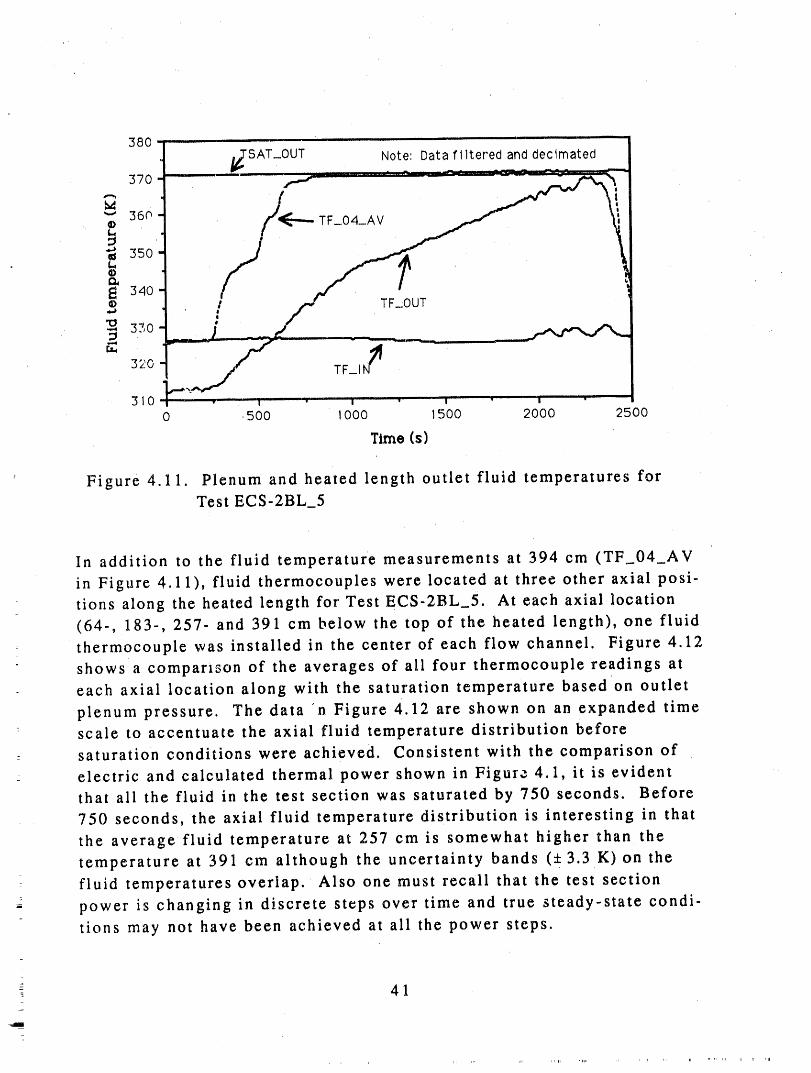
380 ' I'SAT_OUT Note: Data filtered and decimated

--, 360 ' ,

35O

340 I! TF_OUT

'_ 3.,0= .... / _ L-,' ______ ,..

320 TF_I

310 . i I .i,, I " I i . I "

o ,5oo looo 15oo 2000 2500

Time (s)

' Figure 4.11. Plenum and heated length outlet fluid temperatures forTest ECS-2BL_5

In addition to the fluid temperature measurements at 394 cm (TF_04_AV

in Figure 4.11), fluid thermocouples were located at three other axial posi-

tions along the heated length for Test ECS-2BL_5. At each axial location

(64-, 183-, 257- and 391 cm below the top of the heated length), one fluid

thermocouple was installed in the center of each flow channel. Figure 4.12

shows a comparison of the averages of ali four thermocouple readings at

each axial location along with the saturation temperature based on outlet

plenum pressure. The data 'n Figure 4.12 are shown on an expanded time: scale to accentuate the axial fluid temperature distribution before

saturation conditions were achieved. Consistent with the comparison of

electric and calculated thermal power shown in Figure 4.1, it is evident

that ali the fluid in the test section was saturated by 750 seconds. Before

750 seconds, the axial fluid temperature distribution is interesting in that

the average fluid temperature at 257 cm is somewhat higher than the

temperature at 391 cm although the uncertainty bands (± 3.3 K)on the

fluid temperatures overlap. Also one must recall that the test section

power is changing in discrete steps over time and true steady-state condi-

tions may not have been achieved at ali the power steps.

41

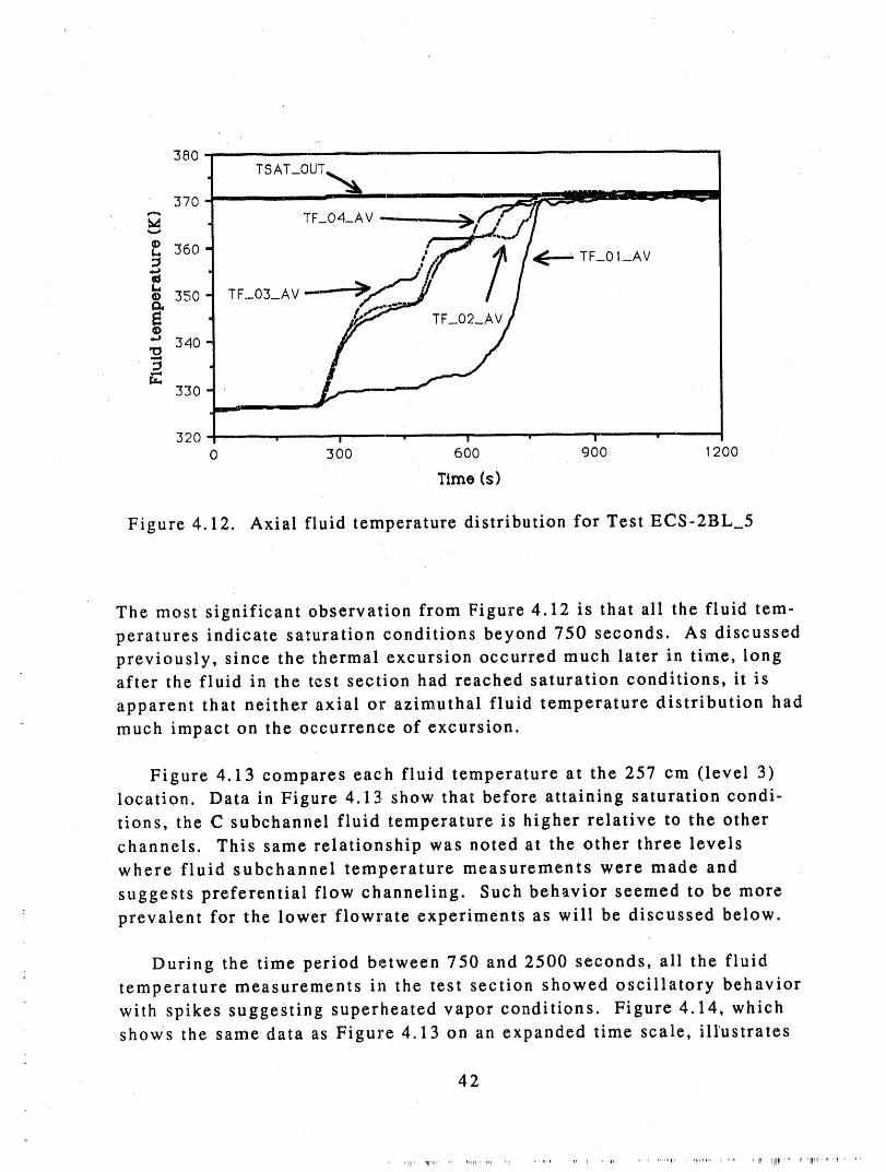
380 ....

TSAT_0UT_, -- , , , ......... II

370 i i -_. --. _

TF_O4_AV Lr.':360 [

TF_OI_AV

350 TF_03_AV

o 340

330 "imiid.I III __ __

320 " " ' I " I ' " I " ---

0 300 600 900 1200

Timo (s)

Figure 4.12. Axial fluid temperature distribution for TestECS-2BL_5

The most significant observation from Figure 4.12 is that all the fluid tem-

peratures indicate saturation conditions beyond 750 seconds, As discussedpreviously, since the thermal excursion occurred much later in time, longafter the fluid in the test section had reached saturation conditions, it is

apparent that neither axial or azimuthal fluid temperature distribution had

much impact on the occurrence of excursion.

Figure 4.13 compares each fluid temperature at the 257 cm (level 3)location. Data in Figure 4.13 show that before attaining saturation condi-tions, the C subchannel fluid temperature is higher relative to the other

channels. This same relationship was noted at the other three levelswhere fluid subchannel temperature measurements were made and

suggests preferential flow channeling. Such behavior seemed to be more

prevalent for the lower flowrate experiments as will be discussed below.

During the time period between 750 and 2500 seconds, all tile fluid

temperature measurements in the test section showed oscillatory behaviorwith spikes suggesting superheated vapor conditions. Figure 4.14, whichshows the same data as Figure 4.13 on an expanded time scale, illustrates

42

'111 Trll,I.... _lll'l lillll , tl IlIItl, i,

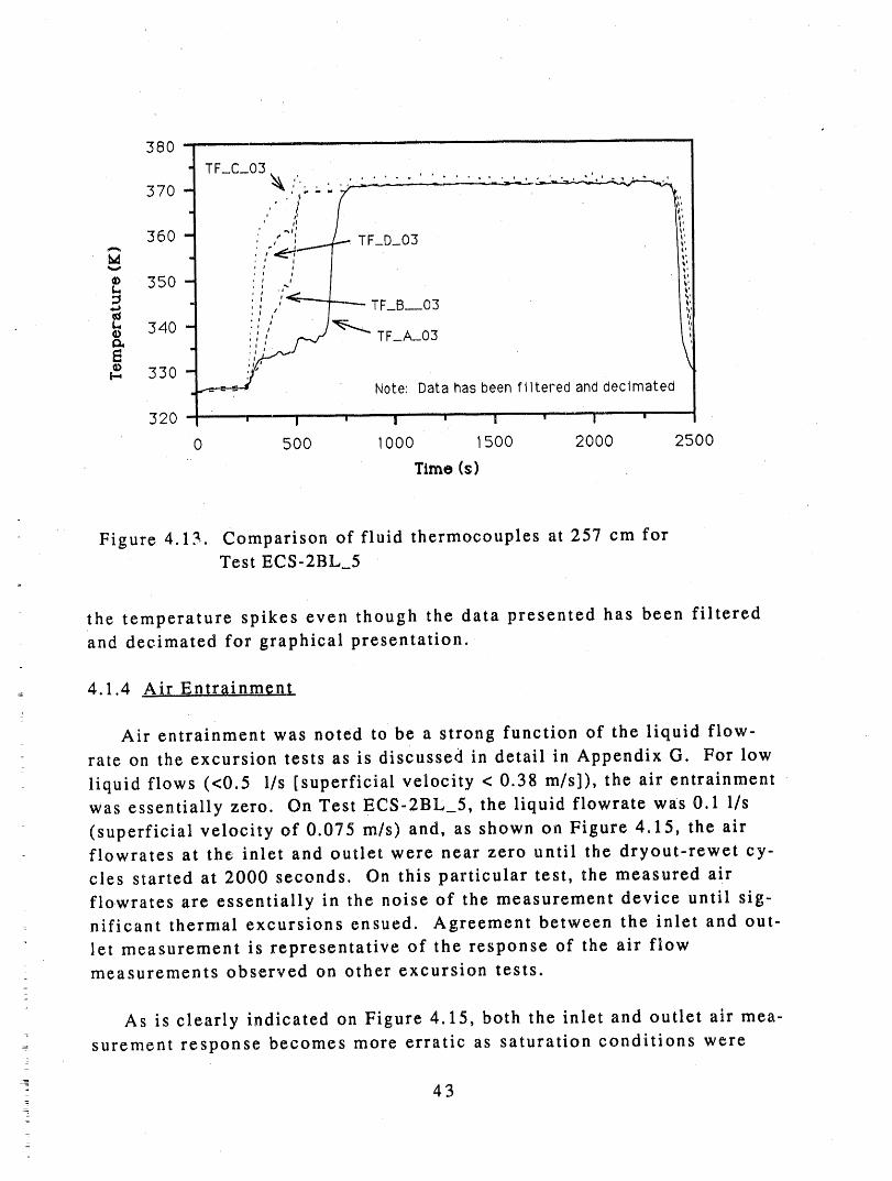
i

380 .........TF_C_03

370 _ ""' ;. ;, - ..... _":'_'_'-_' ' ' ' '"'''' "''

i' ' lt o* li

360 ,_'_, , .- TF_D_03I'

, _o

_, 350 - I .' ',:

.,a ; , -""-- TF_B__03 _:340 - ,, ',',

a, _l _ TF_A_03 l"ml i i

330 -. Note: Data has been filtered and decimated

320 ' I .... ' I ' ' ....... n '" n '

0 500 1000 1500 2000 2500,,

Time (s)

Figure 4.13. Comparison of fluid thermocouples at 257 cm forTest ECS-2BL_5

the temperature spikes even though the data presented has been filtered

and decimated for graphical presentation.

4.1.4 Air Entrainment2

Air entrainment was noted to be a strong function of the liquid flow-

rate on the excursion tests as is discussed in detail in Appendix G. For low

liquid flows (<0.5 l/s [superficial velocity < 0.38 m/si), the air entrainment

was essentially zero. On TestECS-2BL_5, the liquid flowrate was 0.1 1/s

(superficial velocity of 0.075 m/s) and, as shown on Figure 4.15, the air

flowrates at the inlet and outlet were near zero until the dryout-rewet cy-

cles started at 2000 seconds. On this particular test, the measured air

flowrates are essentially in the noise of the measurement device until sig-

nificant thermal excursions ensued. Agreement between the inlet and out-

let measurement is representative of the response of the air flowmeasurements observed on other excursion tests.

As is clearly indicated on Figure 4.15, both the inlet and outlet air mea-

surement response becomes more erratic as saturation conditions were

43

_

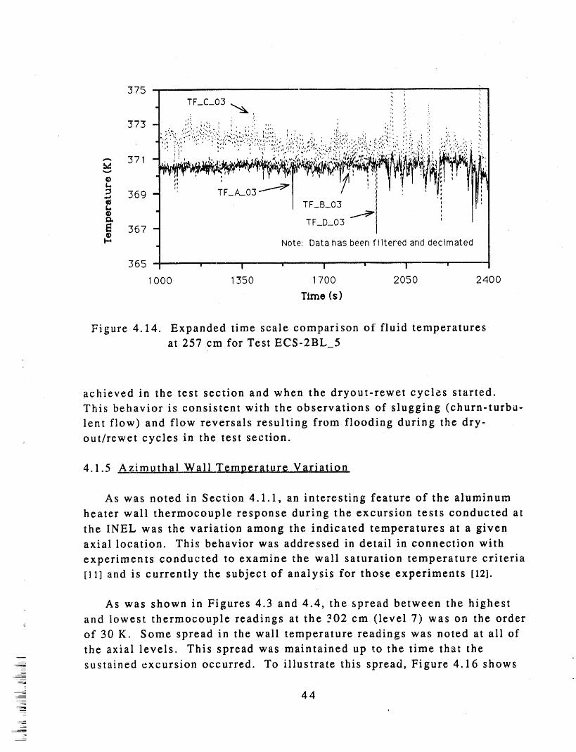
i

375 t ii ,i !iTF_C_03 _ ,, :: ! .,

|. '"'_; '.,,',',,",':_-.',", ,,,C ,,.,',_.,',','.a..... ' .... . , ,.,,.;,,..... ,.... :,,...... ,.. .......,, ,,;, ,,,,',,..,,,....... ,... ,,, .,: ..,,,,,.,,,,,:..,_.:, ,.,,.,_ '.,. ,, ,,, ,_ _ :,',,::',I .... , • ,," '.".,',' ,',..',.,...._.," '"' '"" ' " ' " ......... ' .... ' '""" ""_' "'"""' "' ",,'.,,i,":1',,',,"'.' '., ..':, ,,., , _..,.:, ,,',, ' '.

' i:' ' ' _ :"; ,'"' ',,"'" "',_.,,:'.",i! ,,':,';r_" ',..,.'.;, j_.,i,.,_..j,,.,, _ _'_','_':_._11, ,, ,' , .,,, ',,371

° I IIWI't. _J

:_ 369 - li TF-.A-03 _ /¢. TF_B_03 I

' TF_D._03367 -Note: Data has been filtered and decimated

365 ' I ' I' " 'i '

1000 1350 1700 2050 2400

Time (s)

Figure 4.14. Expanded time scale comparison of fluid temperaturesat 257 cm for Test ECS-2BL_5

achieved in the test section and when the dryout-rewet cycles started.

This behavior is consistent with the observations of slugging (churn-turbid-

lent flow) and flow reversals resulting from flooding during the dry-

. out/rewet cycles in the test section.

4.1.5 Az.__,im_hal Wall Temp_ratur¢_ Variation

As was noted in Section 4.1.1, ;in interesting feature of the aluminum

heater wall thermocouple response during the excursion tests conducted at

the INEL was the variation among the indicated temperatures at a givenaxial location. This behavior was addressed in detail in connection with

experiments conducted to examine the wall saturation temperature criteria[11] and is currently the subject of analysis for those experiments [12].

As was shown in Figures 4.3 and 4.4, the spread between the highest

and lowest thermocouple readings at the 302 cm (level 7) was on the order

of 30 K. Some spread in the wall temperature readings was noted at ali of

the axial levels. This spread was maintained up to the time that the

--_ sustained excursion occurred. To illustrate this spread, Figure 4.16 shows

44

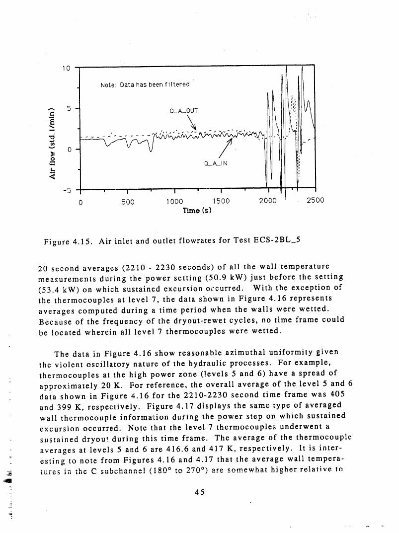
0 ,.iii i, ii ii

Note: Data has beenfiltered

5 i pl I

,,iiil i irl

• J:--- o :i

<, i

-5 .......... ' - I " ........... _ _

0 500 1000 1500 2000 2500Time (s)

Figure 4.15. Air inlet and outlet flowrates for Test ECS-2BL_5

20 second averages (2210 - 2230 seconds) of all the wall temperature

measurements during the power setting (50.9 kW) just before the setting

(53.4 kW) on which sustained excursion occurred. With the exception of

the thermocouples at level 7, the data shown in Figure 4.16 represents

averages computed during a time period when the walls were wetted.

Because of the frequency of the dryout-rewet cycles, no time frame could

be located wherein ali level 7 thermocouples were wetted.

The data in Figure 4.16 show reasonable azimuthal uniformity given

the violent oscillatory nature of the hydraulic processes. For example,

thermocouples at the high power zone (levels 5 and 6) have a spread of_

approximately 20 K. For reference, the overall average of the level 5 and 6

data shown in Figure 4.16 for the 2210-2230 second time frame was 405

and 399 K, respectively. Figure 4.17 displays the same type of averaged

wall thermocouple information during the power step on which sustained

excursion occurred. Note that the level 7 thermocouples underwent a

sustained dryout during this time frame. The average of the thermocouple

averages at levels 5 and 6 are 416.6 and 417 K, respectively, lt is inter-

esting to note from Figures 4.16 and 4.17 that the average wall tempera-- ..,_._ /180 o o70 °__ tures iF, the C _,._,_,..anncl _ to _ ) are somewhat higher re!afire to

45

_

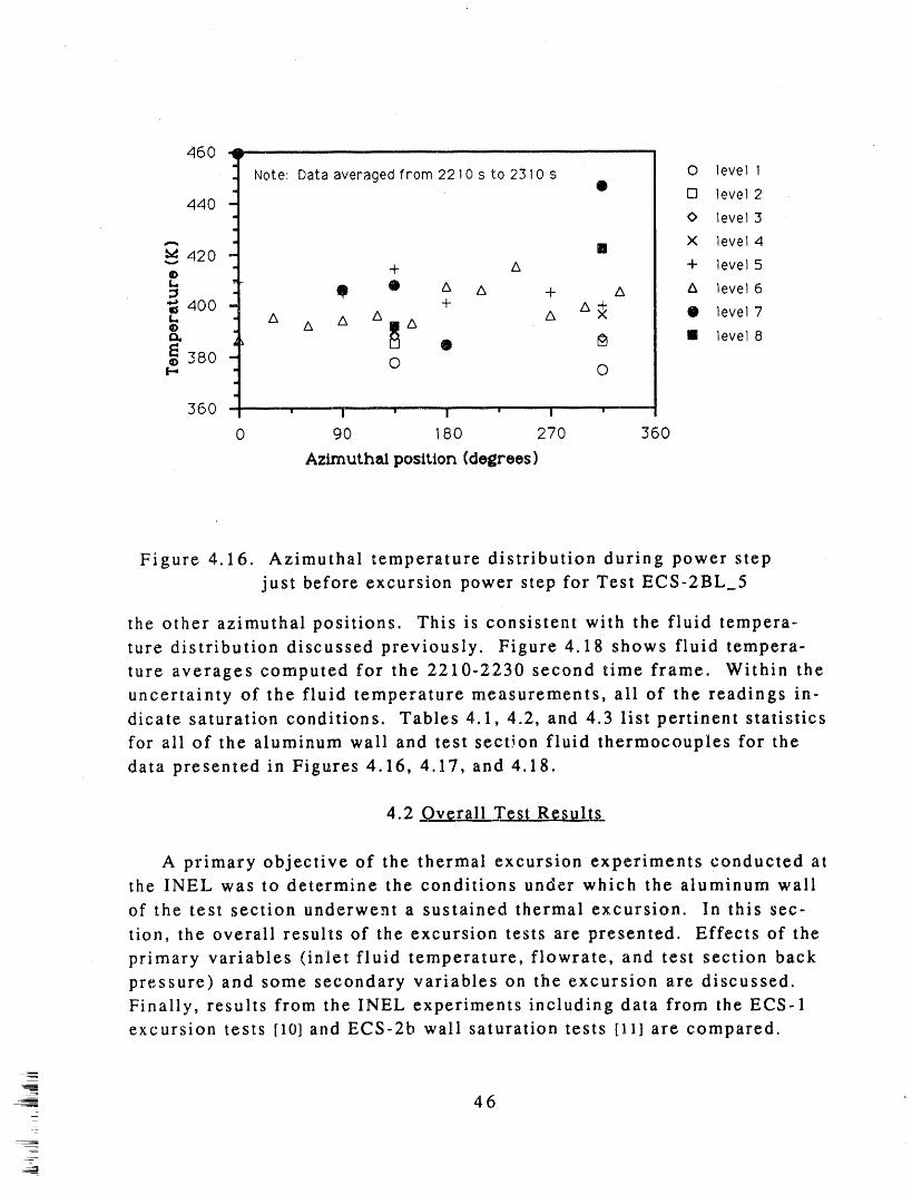
460 4

Note: Data averaged from 2210s to 2310 s 0 level 1Q [] level 2

4400 level 3

X level 4420 II

• + A + level 5• /k A level 6

"' 400 + A .+. Q level 7L, A A A A ×

• A _A • _ I level 8380© 0 0

360 ' ' "'-] - ' 'n , u , '

0 90 180 270 360

Azimuthal position (dogrees)

Figure 4.16. Azimuthal temperature distribution during power step

just before excursion power step for Test ECS-2BL_5

the other azimuthal positions. This is consistent with the fluid tempera-

ture distribution discussed previously. Figure 4.18 shows fluid tempera-

ture averages computed for the 2210-2230 second time frame. Within the

uncertainty of the fluid temperature measurements, ali of the readings in-

dicate saturation conditions. Tables 4.1, 4.2, and 4.3 list pertinent statistics

for ali of the aluminum wall and test section fluid thermocouples for the

data presented in Figures 4.16, 4.17, and 4.18.

4.2 Overall Test Res01ts_

A primary objective of the thermal excursion experiments conducted at

the INEL was to determine the conditions under which the aluminum wall

of the test section underwent a sustained thermal excursion. In this sec-

tion, the overall results of the excursion tests are presented. Effects of the

primary variables (inlet fluid temperature, flowrate, and test section back

pressure) and some secondary variables on the excursion are discussed.

Finally, results from the INEL experiments including data from the ECS-1

excursion tests [10] and ECS-2b wall saturation tests [11] are compared.

4 6

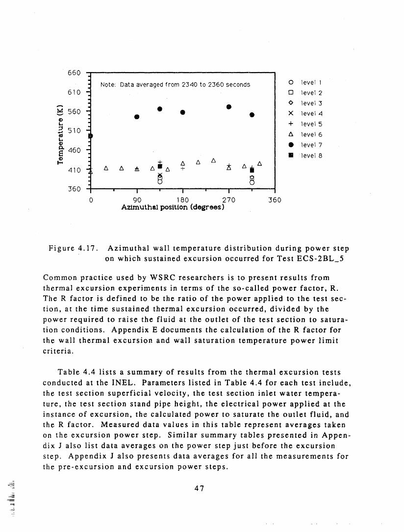
660 ............i

: Note: Data averaged from 2340 to 2360 seconds 0 level 1610 _ 1:3 level 2ml

,,i

- O level 3

s6o - • • •© . • • X level 4

: + level 53 -

! A level 6© " @ level 7l_ 460 -© I level 8

. _ A A A410 "_ & & _ _ A + _ Ai

8360 " ' I " ' I '" ' ' I '_ "

0 90 180 270 360Azimuthal position (degrees)

Figure 4.17. Azimuthal wall temperature distribution during power step

on which sustained excursion occurred for Test ECS-2BL_5

Common practice used by WSRC researchers is to present results from

thermal excursion experiments in terms of the so-called power factor, R.

The R factor is defined to be the ratio of the power applied to the test sec-

tion, at the time sustained thermal excursion occurred, divided by the

power required to raise the fluid at the outlet of the test section to satura-

tion conditions. Appendix E documents the calculation of the R factor for

the wall thermal excursion and wall saturation temperature power limit

criteria.

Table 4.4 lists a summary of results from the thermal excursion tests

conducted at the INEL. Parameters listed in Table 4.4 for each test include,

the test section superficial velocity, the test section inlet water tempera-

ture, the test section stand pipe height, the electrical power applied at the

instance of excursion, the calculated power to saturate the outlet fluid, and

the R factor. Measured data values in this table represent averages taken

on the excursion power step. Similar summary tables presented in Appen-

dix J also list data averages on the power step just before the excursion

step. Appendix J also presents data averages for all the measurements for

the pre-excursion and excursion power steps.

_

47

, . ,, ,,

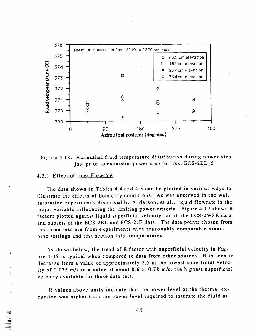
376 ..........

- Note: Data averagedfrom 2210 to 2230 seconds

375 -- 0 63,5 cmelevation

[] 183cm elevation"-" 374 --© 0 257 cm elevation

*,:J 373 -- [] X 394 cm elevation

© 372 -- 0

© 0--_ 371 -- 0 O _ I___ . []

0370 -- X X !_

" x369 ' 'i ' -Ii, , i ' ---

0 90 180 270 360

Azimuthal position (degrees)

Figure 4.18. Azimuthal fluid temperature distribution during power stepjust prior to excursion power step for Test ECS-2BL_5

4.2.1 Effect of Inlet Flowrat¢

The data shown in Tables 4.4 and 4.5 can be plotted in various ways to

illustrate the effects of boundary conditions. As was observed in the wall

saturation experiments discussed by Anderson, et al., liquid flowrate is the

major variable influencing the limiting power criteria. Figure 4.19 shows R

, factors plotted against liquid superficial velocity for all the ECS-2WSR dataand subsets of the ECS-2BL and ECS-2cE data. The data points chosen from

the three sets are from experiments with reasonably comparable stand-

pipe settings and test section inlet temperatures.

As shown below, the trend of R factor with superficial velocity in Fig-

ure 4-19 is typical when compared to data from other sources. R is seen to

decrease from a value of approximately 2.5 at the lowest superficial veloc-

: ity of 0.075 m/s to a value of about 0.6 at 0.78 m/s, the highest superficialvelocity available for these data sets.

R values above unity indicate that the power level at the thermal ex-_

cursion was higher than the power level required to saturate the fluid at

AO"'i'U

_

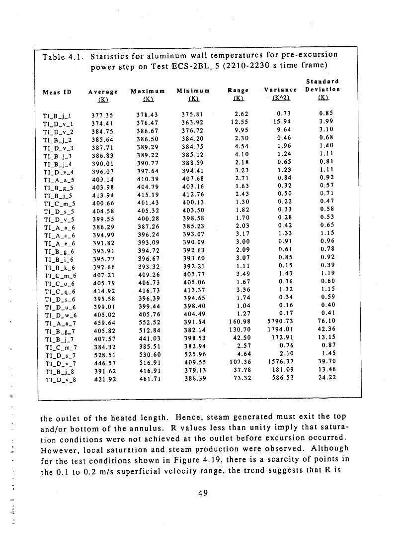
Table 4.1. Statistics for aluminum wall temperatures for pre-excursion

power step on Test ECS-2BL 5 (2210-2230 s time frame)

Standard

Meas lD Average Maximum Minimum Range Variance Deviation

TI_B..j_I 377.35 378.43 375.81 2.62 0.73 0.85

TI_D_v_I 374.41 376.47 363.92 12.55 15.94 3.99

TI_D_v_2 384.75 386.67 376.72 9.95 9.64 3.10

TI_B_j_2 385.64 386.50 384.20 2.30 0.46 0.68TI_D_v_3 387.71 389.29 384,75 4.54 1.96 1.40

TI_B_j_3 386.83 389.22 385.12 4.10 1.24 1.11

TI_B_j_4 390.01 390.77 388.59 2.18 0.65 0.81

TI_D_v_4 396.07 397.64 394.41 3.23 1.23 1.11TI_A_a_5 409.14 410.39 407,68 2.71 0.84 0.92

TI_B_g_5 403.98 404.79 403.16 1.63 0.32 0.57TI_B_j_5 413.94 415.19 412.76 2.43 0.50 0.71TI C m_5 400.66 401.43 400.13 1.30 0.22 0.47TI_D_s_5 404.58 405.32 403.50 1.82 0.33 0.58TI_D_v_5 399,55 400.28 398.58 1.70 0.28 0.53TI A_a_6 386.29 387,26 385.23 2.03 0.42 0.65TI_A_c_6 394.99 396,24 393.07 3.17 1.33 1,15

TI_A_e_6 391.82 393.09 390.09 3.00 0.91 0.96TI_B_g_6 393.91 394.72 392,63 2.09 0.61 0,78TI_B_i 6 395.77 396.67 393.60 3.07 0.85 0,92TI_B_k_6 392,66 393.32 392.21 1.11 0.15 0.39TI C m 6 407.21 409 26 405.77 3.49 1,43 1.1,9

TI_C_o 6 405.79 406 73 405.06 1.67 0.36 0,60TI_C_q_6 414.92 416 73 413.37 3.36 1.32 1.15TI_D_s_6 395.58 396 39 394,65 1.74 0.34 0.59TI_D_u_6 399.01 399 44 398.40 1.04 0.16 0.40TI_.D_w_6 405.02 405 76 404.49 1.27 0.17 0.41TI_A_a_7 459.64 552 52 391.54 160.98 5790.73 76,10

TI_B_g_7 405.82 512 84 382.14 130 70 1794.01 42.36TI_B_j 7 407.57 441 03 398.53 42.50 172.91 13.15TI_C_m 7 384.32 385.51 382.94 2.57 0.76 0,87TI_D_s_7 528.51 530.60 525.96 4.64 2.10 1.45TI_D_v 7 446.57 516,91 409.55 107.36 1576,37 39.70

TI_B_j 8 391.62 416.91 379.13 37.78 181.09 13,46TI_D v_8 421.92 461.71 388.39 73.32 586.53 24,22

the outlet of the heated length. Hence, steam generated must exit the top

and/or bottom of the annulus. R values less than unity imply that satura-- tion conditions were not achieved at the outlet before excursion occurred.

However, local saturation and steam production were observed. Although

for the test conditions shown in Figure 4.19, there is a scarcity of points in

the 0.1 to 0.2 m/s superficial velocity range, the trend suggests that R is2

49

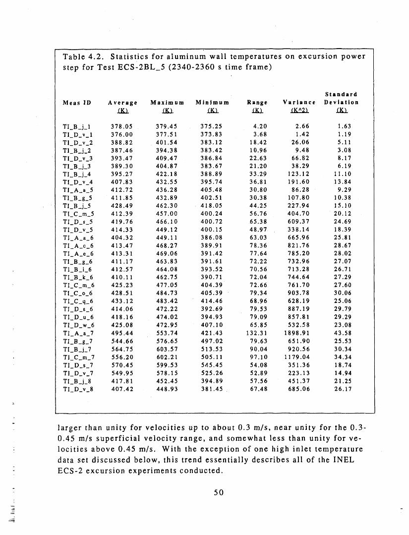
Table 4.2. Statistics for aluminum wall temperatures on excursion power

step for Test ECS-2BL_5 (2340-2360 s time frame)

Standard

Meas lD Average Maximum Minimum Range Variance Deviation

TI_B_j_I 378 05 379 45 375.25 4.20 2.66 1.63TI D v 1 376 00 377 51 373.83 3.68 1.42 1.19TI_D_v_2 388 82 401 54 383.12 18.42 26.06 5.11

TI B_j,2 387 46 394 38 383.42 10.96 9.48 3.08TI_D v_3 393 47 409 47 386 84 22.63 66.82 8.17TI_B_j_3 389 30 404 87 383.67 21.20 38.29 6.19

TI B_j..4 395 27 422 18 388.89 33.29 123.12 11.10TI D v_4 407 83 432 55 395.74 36.81 191.60 13.84TI A a 5 412 72 436 28 405.48 30.80 86.28 9.29TI B_g_5 411 85 432.89 402.51 30.38 107.80 10.38TI_B_j_5 428 49 462.30 418.05 4425 227.94 15.10TI_C_m_5 412.39 457,00 400.24 5676 404.70 20.12

TI_D s_5 419.76 466.10 400.72 65 38 609.37 24,,69TI_D_v_5 414.33 449.12 400.15 4897 338.14 18.39TI_A_a_6 404.32 449.11 386,08 63 03 665.96 25.81TI_A c_6 413.47 468.27 389.91 78 36 821.76 28 67TI_A_e_6 413.31 469.06 391.42 77 64 785.20 28 02TI_B_g_6 411.17 463.83 391.61 72 22 732.96 27 07TI_B_i 6 412.57 464.08 393.52 70 56 713,28 26 71TI_B_k_6 410.11 462.75 390.71 72 04 744.64 27 29

z TI_C_rn_6 425.23 477.05 404.39 72 66 761.70 27 60TI_C_o_6 428.51 484.73 405.39 79 34 903.78 30 06TI_C_q_6 433.12 483.42 414.46 68 96 628.19 25.06TI_D s_6 414.06 472.22 392.69 79 53 887.19 29.79TI_D_u_6 418.16 474.02 394.93 79 09 857.81 29.29TI_D w_6 425.08 472.95 407 10 65 85 532.58 23.08

z

TI_A_a_7 495.44 553.74 421 43 132.31 1898.91 43.58TI_B_g_7 544.66 576.65 497 02 79.63 651,90 25.53TI B_j_7 564.75 603.57 513 53 90.04 920.56 30.34

, TI_C_m_7 556,20 602.21 505 11 97.10 1179.04 34.34TI_D_s_7 570.45 599,53 545 45 54.08 351.36 18.74TI_D_v_7 549.95 578.15 525.26 52.89 223.13 14.94TI_B_j_8 417.81 452.45 394.89 57.56 451.37 21.25TI_D_v_8 407.42 448.93 381.45 67.48 685.06 26.17

larger than unity for velocities up to about 0.3 m/s, near unity for the 0.3-

0.45 rn/s superficial velocity range, and somewhat less than unity for ve-

locities above 0.45 m/s. With the exception of one high inlet temperature

data set discussed below, this trend essentially describes ali of the INEL-

- ECS-2 excursion experiments conducted.

50

.

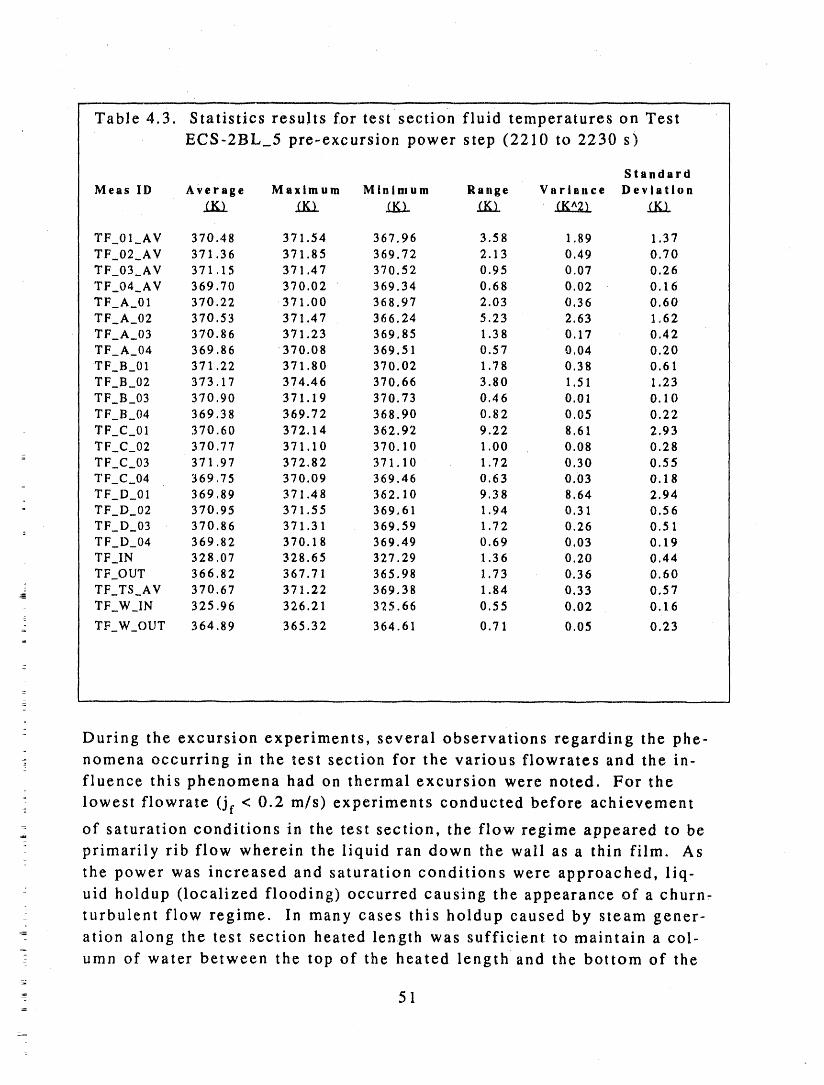
Table 4.3. Statistics results for test section fluid temperatures on Test

ECS-2BL_5 pre-excursion power step (2210 to 2230 s)

Standard

Meas lD Average Maximum Minimum Range Variance DeviationLK3. _ IKL _K_ _

TF_01 AV 370 48 371.54 367.96 3,58 1.89 1.37TF_02_AV 371 36 371.85 369.72 2.13 0.49 0.70TF_03 AV 371 15 371.47 370.52 0.95 0.07 0.26'I'F_04 AV 369 70 370.02 369.34 0.68 0.02 0.16TF_A_01 370 22 371.00 368.97 2.03 0.36 0.60TF_A_02 370 53 371.47 366.24 5.23 2.63 1.'62TF_A_03 370 86 371.23 369.85 1.38 0.17 0.42TF_A._04 369.86 370.08 369.51 0.57 0.04 0.20TF,B_01 371.22 371.80 370.02 1.78 0.38 0.61TF_B_02 373.17 374.46 370.66 3.80 1.51 1.23TF_B_03 370.90 371.19 370.73 0.46 0.01 0.10TF_B_04 369.38 369.72 368.90 0.82 0.05 0.22TF_C 01 370.60 372.14 362.92 9.22 8.61 2.93TF_C_02 370.77 371.10 370.10 1.00 0.08 0 28

-: TF_C_03 371.97 372.82 371.10 1.72 0.30 0 55TF C_04 369.75 370.09 369.46 0.63 0.03 0 18TF_D_01 369.89 371.48 362.10 9.38 8.64 2 94TF_D_02 370.95 371.55 369.61 1.94 0.31 0 56TF_D_03 370.86 371.31 369.59 1.72 0.26 0 517.

TF_D_04 369.82 370.18 369.49 0.69 0.03 0 19TF_IN 328.07 328.65 327.29 1.36 0.20 0 44TF_OUT 366.82 367.71 365.98 1.73 0.36 0 60TF_TS AV 370.67 371.22 369.38 1.84 0.33 057TF_W_IN 325.96 326.21 325.66 0.55 0.02 0.16

TF_W_OUT 364.89 365.32 364.61 0.71 0.05 0.23

-

During the excursion experiments, several observations regarding the phe-

nomena occurring in the test section for the various flowrates and the in-

fluence this phenomena had on thermal excursion were noted. For the

lowest flowrate (if < 0.2 m/s) experiments conducted before achievement

2 of saturation conditions in the test section, the flow regime appeared to beprimarily rib flow wherein the liquid ran down the wall as a thin film. As_

the power was increased and saturation conditions were approached, liq-

uid holdup (localized flooding) occurred causing the appearance of a churn-

turbulent flow regime. In many cases this holdup caused by steam gener-ation along the test section heated length was sufficient to maintain a col-

urnn of water between the top of the heated length and the bottom of the

51

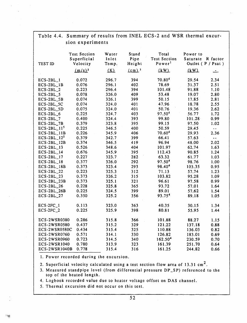
Table 4.4. Summary of results from INELECS-2 and WSR thermal excur-

sion experiments

Test Section Water Stand Total Power to

Superficial Inlet Pipe Test Section Saturate R factorTEST ID Velocity Temp, Height Power 1 Outlet ( P / Psat )

.LmLS.Z2 .CK.)_ L.q_mZ3 _ _kW) -

ECS-2BL_I 0,072 296.7 394 70.804 29,54 2.34ECS-2BL_IB 0.076 296.1 402 78.69 31.37 2,51ECS-2BL_2 0,223 296,4 394 101.48 91,88 1,10ECS-2BL_5 0,078 326.0 409 53.48 19,07 2.80ECS-2BL_SB 0.074 326.1 399 50.15 17.85 2.81ECS-2BL 5C 0.074 324,0 401 47.96 18.78 2.55ECS-2BL_5D 0.075 324.0 401 50,76 19.36 2.62ECS-2B L_6 0.225 324.7 403 97,504 56.77 1.72ECS-2BL_7 0.400 324.4 393 99.80 101,28 0,99ECS-2BL_7B 0,379 323.8 395 99.15 97.50 1.02ECS-2BL_ll 5 0,225 346.5 400 50.59 29.45 --ECS-2BL_ 11B 0,226 345.9 406 70,604 29.93 2.36ECS-2BL_125 0.379 342.7 399 66.41 57.63 --ECS-2BL_12B 0,374 346.5 419 96.94 48.00 2,02ECS-2BL_ 13 0.526 348,6 404 101,97 62.74 1.63ECS-2BL_14 0,676 345.9 395 112.43 90.85 1.24ECS'2BL_I 7 0,227 323.7 282 63.32 61.77 1.03ECS-2BL_18 0,377 326.0 292 97.504 98.76 1.00ECS-2BL_18B 0,373 323.4 293 98.404 103.35 0.95ECS-2BL_22 0,223 325.3 312 71.13 57.74 1.23ECS-2BL_23 0.373 326.2 315 103.82 95.28 1 09ECS-2BL_23B 0.373 325.1 321 96.61 97.58 0.99ECS-2BL_26 0,228 325.8 365 93.72 57.01 1.64ECS-2BL_26B 0.225 324.5 399 89.01 57.62 1.54ECS-2BL 27 0,350 325.2 356 93.754 89.18 1.05

ECS-2FC_I 0,113 323.0 363 40.35 30.15 1,34ECS-2FC_2 0.225 325.9 398 80.81 55.95 1,44

ECS-2WSR0380 0.286 315.8 366 101.88 88.27 1.15ECS-2WSR0580 0.437 315.2 329 121.22 137.18 0.88ECS-2WSR0580C 0.434 315.4 325 110.88 136,03 0.82ECS-2WSR0760 0.571 314.1 330 126,82 183.01 0.69ECS-2WSR0960 0.723 314.5 340 162.504 230.59 0.70ECS-2WSR1040 0,780 313.9 323 161.39 251.70 0.64ECS-2WSR1040B 0,778 315.4 316 161.25 244.82 0.66

1. Power recorded during the excursion.

2. Superficial velocity calculated using a test section flow area of 13.31 cm 2.

3. Measured standpipe level (from differential pressure DP SP) referenced to thetop of the heated length.

4. Logbook recorded value due to heater voltage offset on DAS channel.5. Thermal excursion did not occur on this test.

52

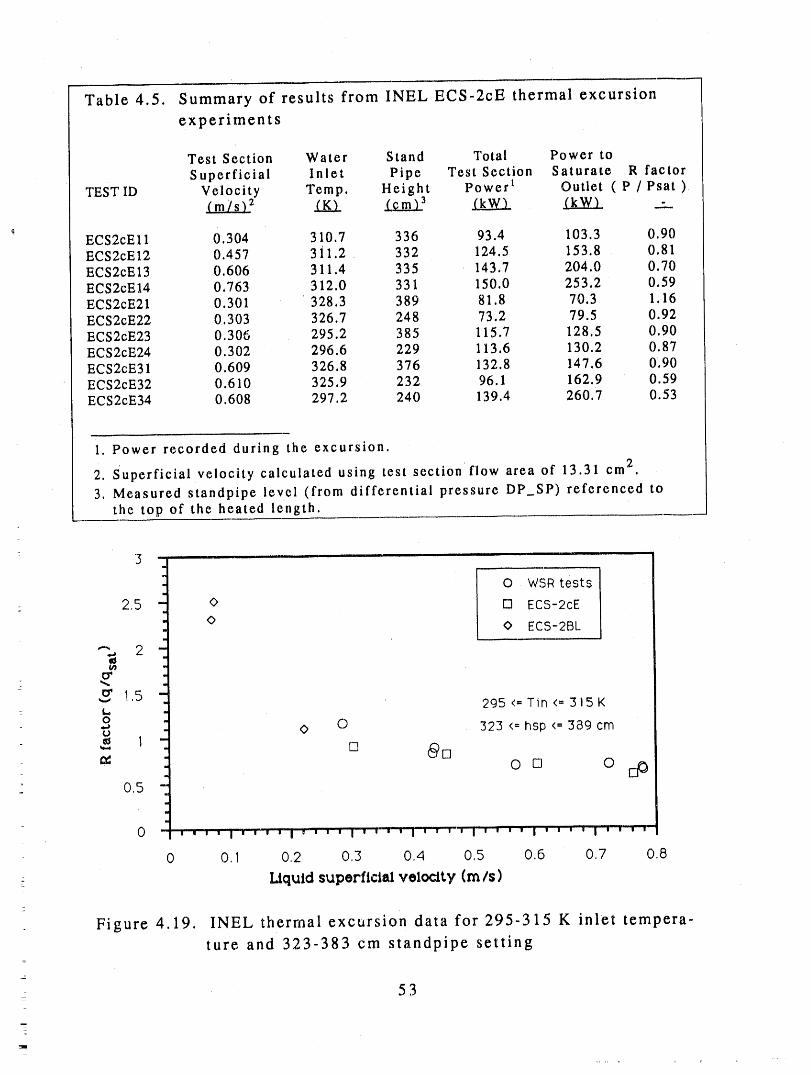
Table 4.5. Summary of results from INEL ECS-2cE thermal excursion

experiments

Test Section Water Stand Total Power to

Superficial Inlet Pipe Test Section Saturate R factorTESTID Velocity Temp. Height Power I Outlet (P /Psat)

(m/s 12 _ (_3 _ (kW,) -

ECS2cE 11 0,304 310.7 336 93.4 103.3 0.90ECS2cE12 0.457 3il.2 332 124,5 153,8 0.81ECS2cEI3 0,606 311,4 335 143.7 204.0 0,70ECS2cE14 0,763 312,0 331 150.0 253.2 0,59ECS2cE21 0.301 328,3 389 81,8 70.3 1.16ECS2cE22 0,303 326.7 248 73,2 79.5 0,92ECS2cE23 0,306 295.2 385 115.7 128.5 0.90ECS2cE24 0.302 296.6 229 113,6 130.2 0.87ECS2cE31 0.609 326,8 376 132,8 147.6 0.90ECS2cE32 0.610 325,9 232 96.1 162.9 0.59ECS2cE34 0,608 297.2 240 139,4 260,7 0.53

1, Power recorded during the excursion.

2. Superficial velocity calculated using test section _flow area of 13.31 cm 2.

3, Measured standpipe level (from differential pressure DP_SP) referenced tothe top of the heated length.

ii i ii iii iii iii . ii iii i

I 0 WSR tests

2,5 o [] ECS-2cE

o 0 ECS-2BL

"" 2

_ 1,5_. 295 <=Tin <=315 Ko.. ©u O 323 <=hsp <= 389 cm

1 ODoe o do

0,5

0 ' ' ' " I r'T". , I * '" ' "I ' ' '"' I ' I ,. I ' '"' ' I '" Iii I 'L1' I I

0 0, I 02 0,3 0,4 0,5 0,6 0,7 0,8

- Liquidsuperficialvelocity(roIs)

Figure 4,19. INEL thermal excursion data for 295-315 K inlet tempera-

ture and 323-383 cm standpipe setting

53

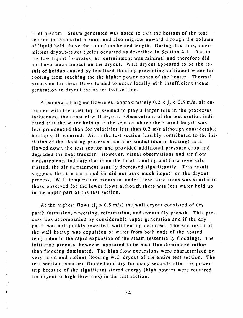
inlet plenum. Steam generated was noted to exit the bottom of the test

section to the outlet plenum and also migrate upward through the column

of liquid held abovethe top of the heated length. During this time, inter-mittent dryout-rewet cycles occurred as described in Section 4.1. Due to

the low liquid flowrates, air entrainment was minimal and therefore did

not have much impact on the dryout. Wall dryout appeared to be the re-

sult of holdup caused by localized flooding preventing sufficient water for

cooling from reaching the the higher power zones of the heater. Thermalexcursion for these flows tended to occur locally with insufficient steam

generation to dryout the entire test section.

At somewhat higher flowrates, approximately 0.2 < jf < 0 5 m/s, air en-

trained with the inlet liquid seemed to play a larger role in the processes

influencing the onset of wall dryout. Observations of the test section indi-

cated that the water holdup in the section above the heated length was

less pronounced than for velocities less than 0.2 m/s although considerable

holdup still occurred. Air in the test section feasibly contributed to the ini-

tiation of the flooding process since it expanded (due to heating) as it

flowed down the test section and provided additional pressure drop and

degraded the heat transfer. However, visual observations and air flow

measurements indicate that once the local flooding and flow reversals

started, the air e_:trainment usually decreased significantly. This result

suggests that the entrained ,tir 0id not have much impact on the dryout

process. Wall temperature excursion under these conditions was similar to

those observed for the lower flows although there was less water held up

in the upper part of the test section.

At the highest flows (if > 0.5 m/s) the wall dryout consisted of dry

patch formation, rewetting, reformation, and eventually growth. This pro-

cess was accompanied by considerable vapor generation and if the dry

patch was not quickly rewetted, wall heat up occurred. The end result of

the wall heatup was expulsion of water from both ends of the heated

length due to the rapid expansion of the steam (essentially flooding). 'File

initiating process, however, appeared to be heat flux dominated rather

than flooding dominated. The high flow excursions were characterized by

very rapid and violent flooding with dryout of the entire test section. The

test section remained flooded and dry for many seconds after the power

trip because of the significant stored energy (high powers were required

for dryout at high flowrates) in the test section.

54

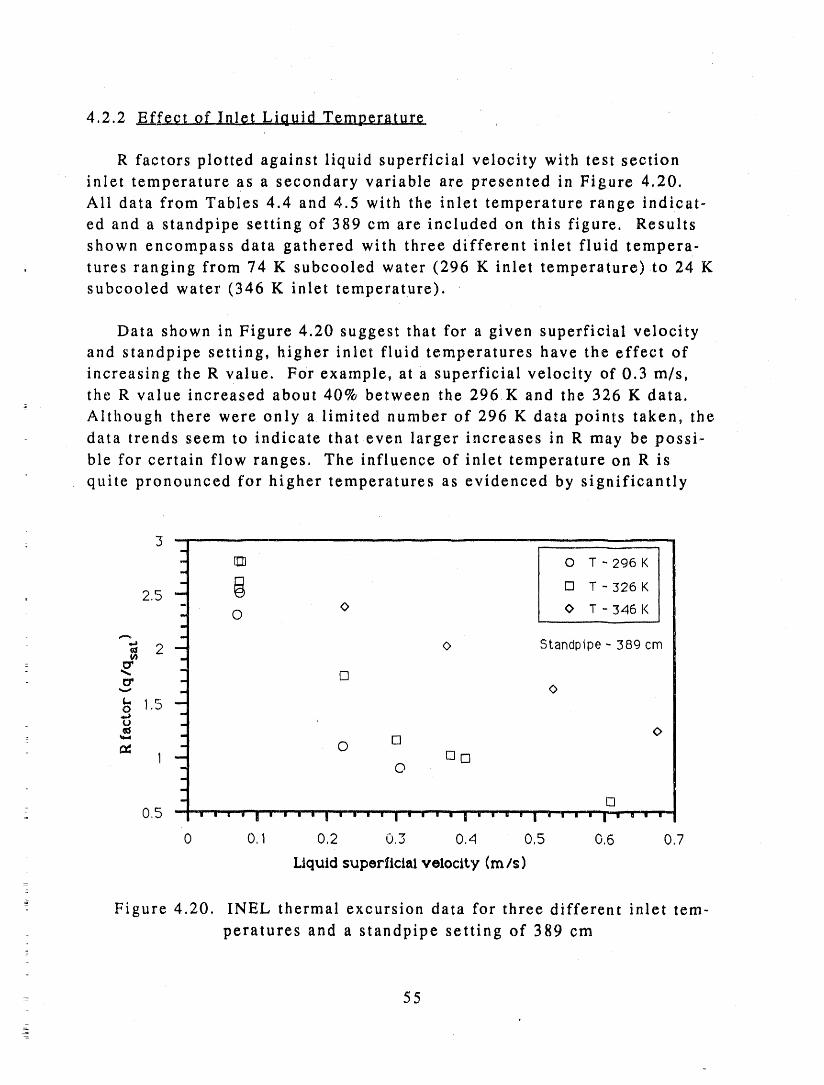
4.2.2 Effect 0f !n!¢t Liquid Temperature

R factors plotted against liquid superficial velocity with test section

inlet temperature as a secondary variable are presented in Figure 4,20.

Ali data from Tables 4.4 and 4.5 with the inlet temperature range indicat-ed and a standpipe setting of 389 cm are included on this figure. Results

shown encompass data gathered with three different inlet fluid tempera-

. tures ranging from 74 K subcooled water (296 K inlet temperature)to 24 K

subcooled water (346 K inlet temperature).

Data shown in Figure 4.20 suggest that for a given superficial velocityand standpipe setting, higher inlet fluid temperatures have the effect of

increasing the R value. For example, at a superficial velocity of 0.3 m/s,the R value increased about 40% between the 296K and the 326 K data.

Although there were only a limited number of 296K data points taken, the

data trends seem to indicate that even larger increases in R may be possi-ble for certain flow ranges. The influence of inlet temperature on R is

quite pronounced for higher temperatures as evidenced by significantly

, i ii,lIi

- [1_ 0 T - 296 Klm

" _ [] T - 326 K__ 2,5 "-

m

- 0 O @ T - 346 Kii

2 -- O Standpipe - 389 cm

- []

t- 15 --0 '

O:- _ ii []

ii 01 -- []E3

- 0u

,a

- E3Illl II li

- 0,5 ' ' ' ' ! ' ' ' ' ! ' " ' ' I ' ' ' • I I'l"'I ILl[ II I ' l I I I _ li • I

0 0,1 0,2 0,3 0,4 0,5 0,6 0,7

Liquid superficial velocity (rn Is)

Figure 4.20. INEL thermal excursion data for three different inlet tem-

peratures and a standpipe setting of 389 cm7

z 55

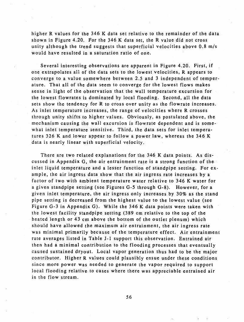
higher R values for the 346 K data set relative to the remainder of the data

shown in Figure 4.20, For the 346K data set, the R value did not cross

unity although the trend suggests that superficial velocities above 0.8 m/swould have resulted in a saturation ratio of one.

Several interesting observations are apparent in Figure 4.20. First, if

one extrapolates ali of the data sets to the lowest velocities, R appears to

converge to a value somewhere between 2.5 and 3 independent of temper-ature. That ali of the data seem to converge for the lowest flows makes

sense in light of the observation that the wall temperature excursion for

the lowest flowrates is domJinated by local flooding. Second, ali thedata

sets show the tendency for R to cross over unity as the flowrate increases.As inlet temperature increases, the range of velocities where R crosses

through unity shifts to higher values. Obviously, as postulated above, the

mechanism causing the wall excursion is flowrate dependent and is some-

what inlet temperature sensitive. Third, the data sets for inlet tempera-tures 326 K and lower appear to follow a power law, whereas the 346 K

data is nearly _.inear with superficial velocity.

There are two related explanations for the 346 K data points. As dis'

cussed in Appendix G, the air entrainment rate is a strong function of the

inlet liquid temperature and a lesser function of standpipe setting. For ex-

ample, the air ingress data show that the air ingress rate increases by a

factor of two with ambient temperature water relative to 346 K water for

a given standpipe setting (see Figures G-5 through G-8). However, for a

given inlet temperature, the air ingress only increases by 30% as the standpipe setting is decreased from the highest value to the lowest value (see

Figure G-3 in Appendix G). While the 346 K data points were taken with

the lowest facility standpipe setting (389 cm relative to the top of the

heated length or 43 cm above the bottom of the outlet plenum) which

should have allowed the maximum air entrainment, the air ingress rate

was minimal primarily because of the temperature effect. Air entrainment

rate averages listed in Table J-1 support this observation. Entrained air

then had a minimal contribution to the flooding processes that eventually

caused sustained dryout. Local vapor generation thus _had to be the major

contributor. Higher R values could plausibly ensue under these conditions

since more power was needed to generate the vapor required to supportlocal flooding relative to cases where there was appreciable entrained airin the flow stream.

56

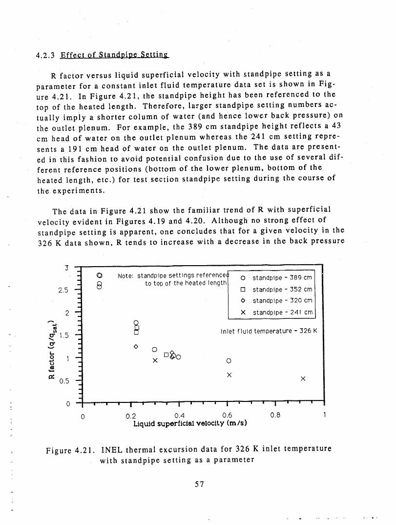
4.2.3 Effg¢_ of Standpipe Setting

R factor versus liquid superficial velocity with standpipe setting as a

parameter for a constant inlet fluid temperature data set is shown in Fig-ure 4.21. In Figure 4.21, the standpipe height has been referenced to the

top of the heated length. Therefore, larger standpipe setting numbers ac-

tually impiy a shorter column of water (and hence lower back pressure) on

the outlet plenum, For example, the 389 cm standpipe height reflects a 43

cm head of water on the outlet plenum whereas the 241 cm setting repre-

sents a 191 cm head of water on the outlet plenum. The data are present-

ed in this fashion to avoid potential confusion due to the use of several dif-

ferent reference positions (bottom of the lower plenum, bottom of the

heated length, etc.) for test section standpipe setting during the course of

the experiments.

The data in Figure 4.21 show the familiar trend of R with superficial

velocity evident in Figures 4.19 and 4.20. Although no strong effect of

standpipe setting is apparent, one concludes that for a given velocity in the

326 K data shown, R tends to increase with a decrease in the back pressure

iill, ,, - , ,, i i,m

- _ Note; standpipe settingsreferencec 0 standpipe- 389cm- _ to top of the heated length

2,5 -: [] standpipe - 3.52 cmm

- O standpipe - 320 cm.i

2 --. X standpipe - 241 cm.._ . 0

tr 1,5 Inlet fluid temperature - 326 Ktr i.

_--, . <)I-. - 0o 1 -- I:l_O-_ X 0U "_1

m

i X0,5 - X

i

,li

0 ' i i " _ 'I i _ _ i i i' i i i '_ . i * I

0 0,2 0,4 0,6 0,8 1I Liquid superficial velocity (mis)

Figure 4.21. INEL thermal excursion data for 326 K inlet temperature

with standpipe setting as a parameter

57

=

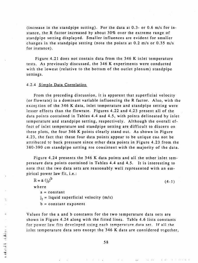
(increase in the standpipe setting). For the data at 0.3- or 0.6 m/s for in-

stance, the R factor increased by about 30% over the extreme range of

standpipe setting displayed. Smaller influences are evident for smallerchanges in the standpipe setting (note the points at 0.2 m/s or 0.35 m/sfor instance).

Figure 4.21 does not contain data from the 346 K inlet temperature

tests. As previously discussed, the 346 K experiments were conducted

with the lowest (relative to the bottom of the outlet plenum) standpipe

settings.

4.2.4 Simple Data Correlation

From the preceding discussion, it is apparent that superficial velocity

(or flowrate) is a dominant variable influencing the R factor. Also, with the

exceI_tion of the 346 K data, inlet temperature and standpipe setting were

lesser effects than the flowrate. Figures 4.22 and 4.23 present ali of the

data points contained in Tables 4.4 and 4.5, with points delineated by inlet

temperature and standpipe setting, respectively. Although the overall ef-

fect of inlet temperature and standpipe setting are difficult to discern on

these plots, the four 346 K points clearly stand out. As shown in Figure

4.23, the fact that these four data points appear to be unique can not be

attribuzed tc back pressure since other data points in Figure 4.23 from the

380-390 cm standpipe setting ere consistent with the majority of the data.

Figure 4.24 presents the 346 K data points and ali the other inlet tem-

perature data points contained in Tables 4.4 and 4.5. It is interesting to

note that the two data sets are reasonably well represented with an em-

pirical power law fit, i.e.'

= a (jl) b (4.. 1 )R

where

a = constant

. jf = liquid superficial velocity (m/s)

b = constant exponent

Values for the a and b constants for the two temperature data sets are

shown in Figure 4.24 along with the fitted lines. Table 4.6 lists constants

f'rar p rauu_r l_Ju flte clevelnpe.rl n¢in, ezeh re.rnpe.ratl_re data ._et. If ali the_

z inlet temperature data sets except the 346 K data are considered together,

58

__

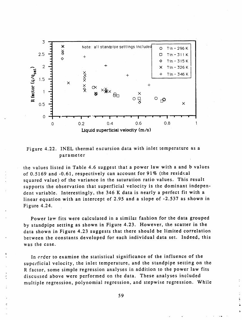
_ --i

" Y_ Note: all standpipe settingsincludec 0 Tin- 296Kv

2,5 i" _ D Tin-311 K- +- O- @ Tin -315 K

A 2 -- + X Tin-326KQID m

. X + Tin - 346 Kt_' . ,_ +1,5---_ _ x

o . _xUa - Qp x0,5 -- xi

wii

i

i

0 " I -- I W I " W ' I II II ' I • l_lI' I II I • i -

0 0,2 0,4 0,6 0.8 1

Liquid superficial velocity (m Is)

Figure 4.22. INEL thermal excursion data with inlet temperature as a

parameter

the values listed in Table 4.6 suggest that a power law with a and b values

of 0.5169 and -0.61, respectively can account for 91% (the resid_;al

squared value) of the variance in the saturation ratio values. This result

supports the observation that superficial velocity is the dominant indepen-dent variable. Interestingly, the 346 K data is nearly a perfect fit with a

linear equation with an intercept of 2.95 and a slope of -2.537 as shown in

Figure 4.24.

Power law fits were calculated in a similar fashion for the data grouped

by standpipe setting as shown in Figure 4.23. However, the scatter in thedata shown in Figure 4.23 suggests that there should be limited correlation

between the constants developed for each individual data set. Indeed, thiswas the case.

: In order to examine the statistical significance of the influence of the

superficial velocity, the inlet temperature, and the standpipe setting on the

R factor, some simple regression analyses in addition to the power law fits=

-- discussed above were performed on the data. These analyses includedr

multiple regression, polynomial regression, and stepwise regression. While

59

irl

:50 Note: all inlet fluid 0 standpipe- 380- 390cm

2.5 _ temperatures included [] standpipe- 352cm= 0 0 0 standpipe-315 - 330cmJ

IN

_-, 2 - 0 x standpipe- 261 cm

_ ." _ + standpipe- 241 cm_ . 0

1.5 -'_.' []

L O ©

ou 18 o

!

o s ¢ +,m

a

I, ii iiJi

0 0.2 0.4 06 08 1

Liquid superficial velocity (m/_)

Figure 4.23. INEl, thermal excursion data with standpipe setting as a

parameter

certainly not an exhaustive investigation of statistical effects, such simple

analyses provide insight on the relative importance of the independent

variables. Furthermore, it was not expected that any of the additional re-

gression ;echniques applied here would necessarily provide a better (or

even as good as) fit of the data relative to the simple power law and such

was found to be the case.

Multiple regression of the data produced an equation of the form"

R =a o +alJ f+a 2 Tin +a 3 hsp (4-2)

where

= -2.446a o

a = -1.7661

a = 0.0092

° a = 0.0043

%i

60

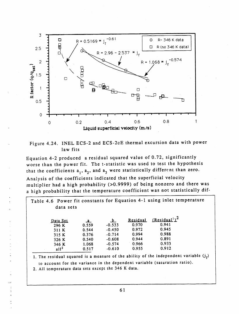
,, i i i ,, ii il i i HI roll m

D R = 0,5169 * jr-0.61 0 R- 346 K data

2,5 " _ /_ 12 R(no 346 Kdata)L-J\ R =2,96-2.537 *jr -- - "

2 . jf-0,574... 68

"- 1,5

t.,

,,o 1u

os

0 ' ii ]_ I ' IlI_ | l _ ' I ' I I I I ' II ' I ' ' I Iii

0 0,2 0,4 0,6 0,8 1

' Liquid superficia! velocity (m/s)

Figure 4.24. INEL ECS-2 and ECS-2cE thermal excursion data with power

law fits

Equation 4-2 produced a residual squared value of 0.72, significantly

worse than the power fit. The t-statistic was used to test the hypothesis

that the coefficients a 1, a 2, and a 3 were statistically different than zero.

Analysis of the coefficients indicated that the superficial velocity

multiplier had a high probability (>0.9999) of being nonzero and there was

a high probability that the temperature coefficient was not statistically dif-

: Table 4.6 Power fit constants for Equation 4-1 using inlet temperature

= data sets

: Data S_.L _L. _h.. __ (Residual1.)_ 2- 296 K 0.559 -0.533 0.970 0.941

: 311 K 0.544 -0.450 0.972 0.945315 K 0.376 -0.714 0.994 0.988326 K 0.540 -0.608 0.944 0.891346 K 1.068 -0.574 0.966 0.933ali 2 0.517 -0.610 0.955 0.912

1. The residual squared is a measure of the ability of the independent variable (jf)

to account for the variance in the dependent variable (saturation ratio).

2. Ali temperature data sets except the 346 K data.

i,. I

61

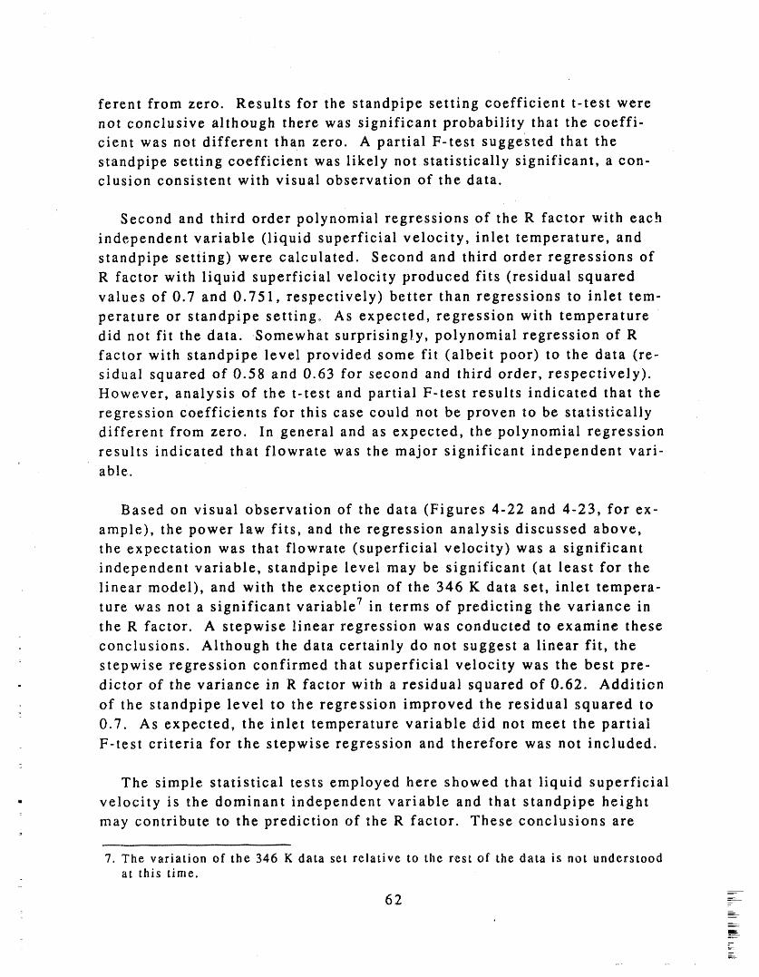
ferent from zero. Results for the standpipe setting coefficient t-test were

not conclusive although there was significant probability that the coeffi-

cient was not different than zero. A partial F-test suggested that the

standpipe setting coefficient was likely not statistically significant, a con-clusion consistent with visual observation of the data.

Second and third order polynomial regressions of the R factor with each

independent variable (liquid superficial velocity, inlet temperature, and

standpipe setting) were calculated. Second and third order regressions of

R factor with liquid superficial velocity produced fits (residual squared

values of 0.7 and 0.751, respectively) better than regressions to inlet tem-

perature or standpipe setting° As expected, regression with temperaturedid not fit the data. Somewhat surprisingly, polynomial regression of R

factor with standpipe level provided some fit (albeit poor) to the data (re-

sidual squared of 0.58 and 0.63 for second and third order, respectively).

However, analysis of the t-test and partial F-test results indicated that the

regression coefficients for this case could not be proven to be statisticallydifferent from zero. In general and as expected, the polynomial regression

results indicated that flowrate was the major significant independent vari-able.

Based on visual observation of the data (Figures 4-22 and 4-23, for ex-

ample), the power law fits, and the regression analysis discussed above,

the expectation was that flowrate (superficial velocity) was a significant

independent variable, standpipe level may be significant (at least for the

linear model), and with the exception of the 346 K data set, inlet tempera-

ture was not a significant variable 7 in terms of predicting the variance in

the R factor. A stepwise linear regression was conducted to examine these

conclusions. Although the data certainly do not suggest a linear fit, the

stepwise regression confirmed that superficial velocity was the best pre-

- dictor of the variance in R factor with a residual squared of 0.62. Addition

of the standpipe level to the regression improved the residual squared to

0.7. As expected, the inlet temperature variable did not meet the partial

F-test criteria for the stepwise regression and therefore was not included.

The simple statistical tests employed here showed that liquid superficial

- velocity is the dominant independent variable and that standpipe height

may contribute to the prediction of the R factor. These conclusions are_

7. The variation of the 346 K data set relative to the rest of the data is not understoodat this time.

62

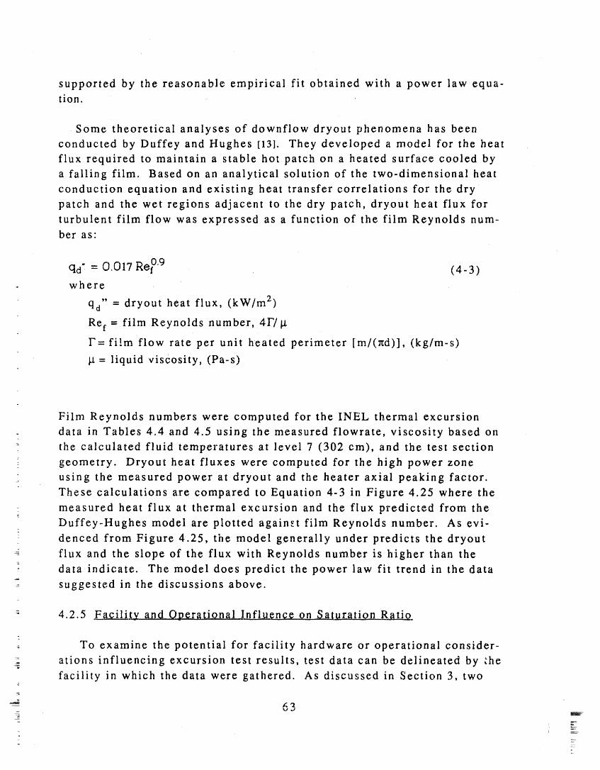
supported by the reasonable empirical fit obtained with a power law equa-tion.

Some theoretical analyses of downflow dryout phenomena has been

conducted by Duffey and Hughes [131, They developed a model for the heat

flux required to maintain a stable hot patch on a heated surface cooled by

a falling film. Based on an analytical solution of the two-dimensional heat

conduction equation and existing heat transfer correlations for the dry

patch and the wet regions adjacent to the dry patch, dryout heat flux for

turbulent film flow was expressed as a function of the film Reynolds num-ber as:

qd" = 0.017 Re °9 (4- 3 )- where

qd = dryout heat flux, (kW/m 2)

Ref = film Reynolds number, 4F/kt

F= fi!m flow rate per unit heated perimeter [m/(_d)], (kg/m-s)

kt = liquid viscosity, (Pa-s)

Film Reynolds numbers were computed for the INEL thermal excursion

o data in Tables 4.4 and 4.5 using the measured flowrate, viscosity based on

the calculated fluid temperatures at level 7 (302 cm), and the test section

geometry. Dryout heat fluxes were computed for the high power zone

using the measured power at dryout and the heater axial peaking factor.

These calculations are compared to Equation 4-3 in Figure 4.25 where the

measured heat flux at thermal excursion and the flux predicted from the

Duffey-Hughes model are plotted against film Reynolds number. As evi-

denced from Figure 4.25, the model generally under predicts the dryout

- flux and the slope of the flux with Reynolds number is higher than the

data indicate. The model does predict the power law fit trend in the data

--- suggested in the discussions above.

-_ 4.2.5 __and Operational In_.f.!._ence on Saturation Ra_.

-

To examine the potential for facility hardware or operational consider-

ations influencing excursion test results, test data can be delineated by _he

facility in which the data were gathered. As discussed in Section 3, two

--_ 6 3-7

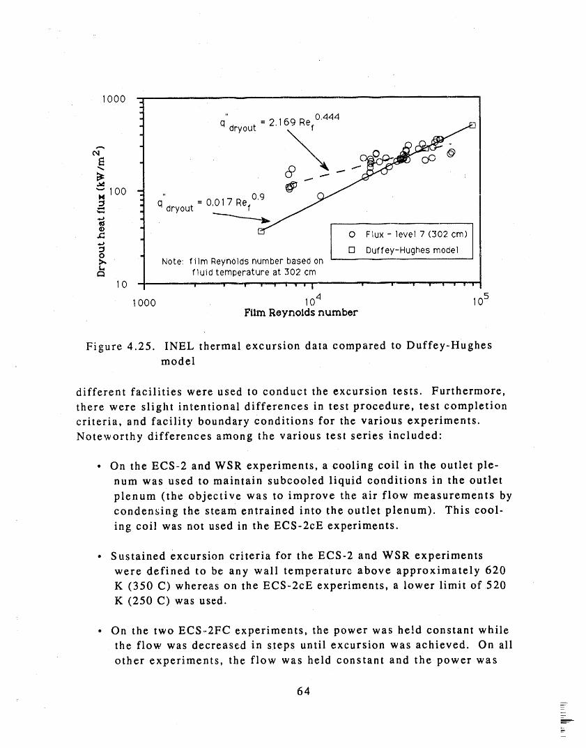
1000 _ ........iiii,

q"dryout = 2.169 Ref 0'444 _)

it

_ _ ,

_" , ,

q dryout = 0

._ 0 Flux - level 7 (302 cm)

o_ [] Duffey-Hughes modelNote: film Reynolds number based on

fluid temperature at 302 cm

10 "....._ ..... , ----J I ' [ I ' I I ' I I ' I ' '

t000 104 10sFilmReynoldsnumber

Figure 4.25. INEL thermal excursion data compared to Duffey-Hughesmodel

different facilities were used to conduct the excursion tests. Furthermore,

there were slight intentional differences in test procedure, test completioncriteria, and facility boundary conditions for the various experiments.

Noteworthy differences among the various test series included"

• On the ECS-2 and WSR experiments, a cooling coil in the outlet ple-

num was used to maintain subcooled liquid conditions in the outlet

plenum (the objective was to improve the air flow measurements by

condensing the steam entrained into the outlet plenum). This cool-

ing coil was not used in the ECS-2cE experiments.

• Sustained excursion criteria for the ECS-2 and WSR experiments

were defined to be any wall temperature above approximately 620K (350 C) whereas on the ECS-2cE experiments, a lower limit of 520

K (250 C) was used.z

° On the two ECS-2FC experiments, the power was held constant while

the flow was decreased in steps until excursion was achieved. On all

other experiments, the flow was held constant and the power was

64

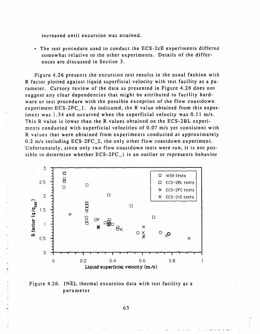
increased until excursion was attained.

• The test procedure used to conduct the ECS-2cE experiments differed

somewhat relative to the other experiments. Details of the differ-ences are discussed in Section 3.

Figure 4.26 presents the excursion test results in the usual fashion with

R factor plotted against liquid superficial velocity with test facility as a pa-rameter. Cursory review of the data as presented in Figure 4.26 does not

suggest any clear dependencies that might be attributed to facility hard-ware or test procedure with the possible exception of the flow coastdown

experimentECS-2FC,1. As indicated, the R value obtained from this exper-

iment was 1.34 and occurred when the superficial velocity was 0.11 m/s.

This R value is lower than the R values obtained on the ECS-2BL experi-

ments conducted with superficial velocities of 0.07 m/s yet consistent with

R values that were obtained from experiments conducted at approximately

0.2 m/s including ECS-2FC 2, the only other flow coastdown experiment.

Unfortunately, since only two flow coastdown tests were run, it is not pos-

sible to determine whether ECS-2FC_I is an outlier or represents behavior

i ....

I_ 0 WSR testsrq

2,5 _ [] ECS-2BL testsD

: [] 0 ECS-2FC tests

2 [] X ECS-2cEtests

u' 15a' o

--_ [] []

[]- ,," Ox x

ox oos xO x

=

i ii ,1 ii i ........ i iii i' -' ' I ' " " I ' ' ' I ' ' ' I ' ' '

0 0.2 0,4 0,6 0,8 1

. Liquid superficial velocity (rn Is)

Figure 4°26. INEL thermal excursion data with test facility as a_

parameter-

65

__

-_

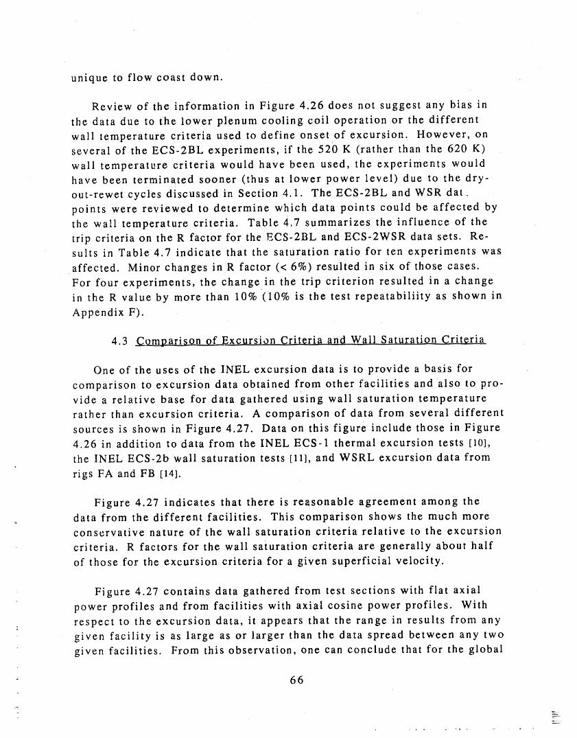
unique to flow coast down.

Review of the information in Figure 4,26 does not suggest any bias in

the data due to the lower plenum cooling coil operation or the different

wall temperature criteria used to define onset of excursion. However, onseveral of the ECS-2BL experiments, if the 520 K (rather than the 620 K)

wall temperature criteria would have been used, the experiments wouldhave been terminated sooner (thus at lower power level) due to the dry-

out-rewet cycles discussed in Section 4.1. The ECS-2BL and WSR dat.

points were reviewed to determine which data points could be affected by

the wall temperature criteria, Table 4.7 summarizes the influence of the

trip criteria on the R factor for the ECS-2BL and ECS-2WSR data sets. Re-suits in Table 4.7 indicate that the saturation ratio for ten experiments was

affected. Minor changes inR factor (.<.6%) resulted in six of those cases.

For four experiments, the change in the trip criterion resulted in a change

in the R value by more than 10% (10% is the test repeatabiliity as shown in

Appendix F).

4.3 _C_.o.._.map_.L_Ex¢0rsion Criteria _nd Wall Saturation Criteria

One of the uses of the INEL excursion data is to provide a basis for

comparison to excursion data obtained from other facilities and also to pro-vide a relative base for data gathered using wall saturation temperature

rather than excursion criteria. A comparison of data from several different

sources is shown in Figure 4.27. Data on this figure include those in Figure4.26 in addition tO data from the INEL ECS-1 thermal excursion tests [10],

the INEL ECS-2b wall saturation tests [11], and WSRL excursion data from

rigs FA and FB [14].

Figure 4.27 indicates that there is reasonable agreement among thedata from the different facilities. This comparison shows the much more

conservative nature of the wall saturation criteria relative to the excursion

criteria. R factors for the wall saturation criteria are generally about half

of those for the excursion criteria for a given superficial velocity.

Figure 4.27 contains data gathered from test sections with flat axial

power profiles and from facilities with axial cosine power profiles. With

respect to the excursion data, it appears that the range in results from any

given facility is as large as or larger than the data spread between any two

given facilities. From this observation, one can conclude that for the global

-_ 66

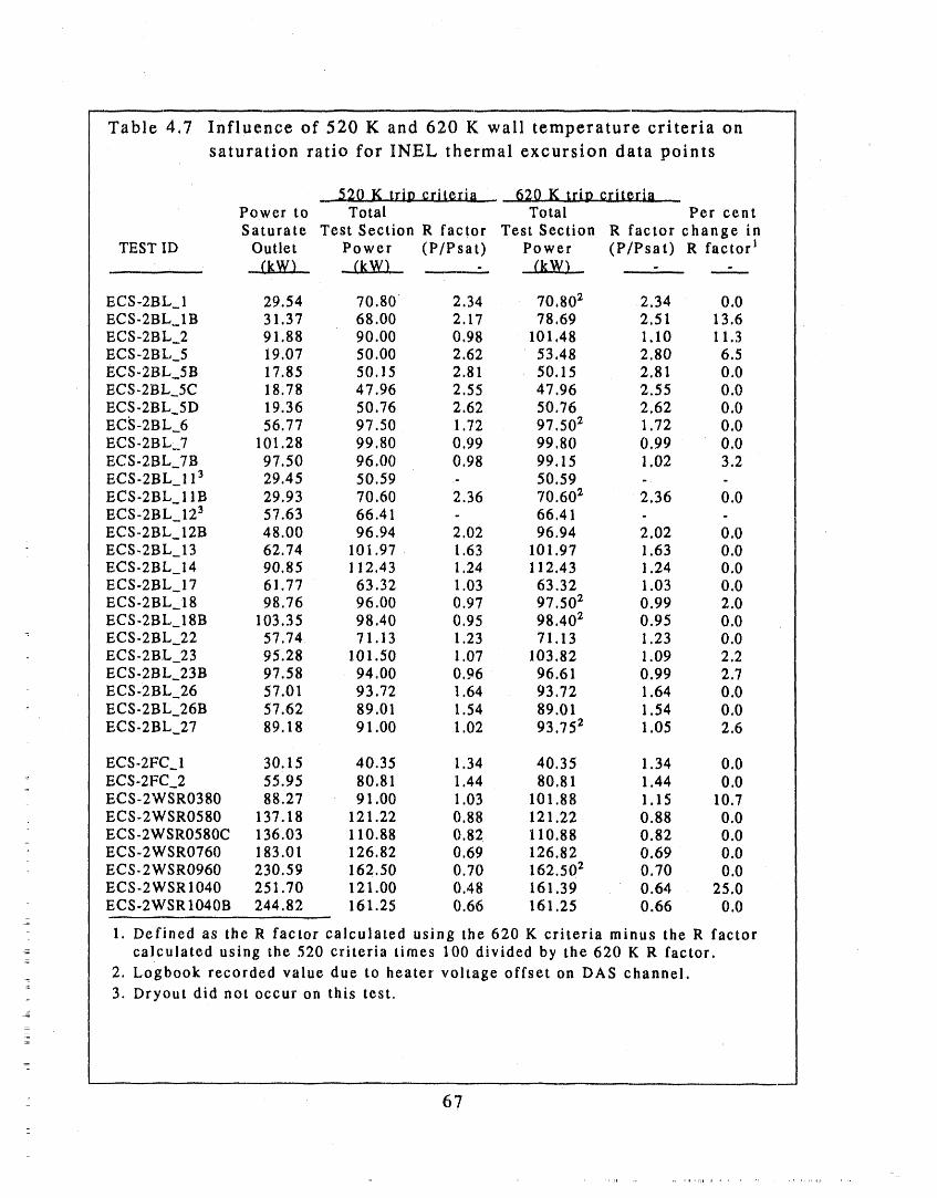
Table 4.7 Influence of 520 K and 620 K wall temperature criteria on

saturation ratio for INEL thermal excursion data points

520 K trip criteria 620 K trio criteriaPower to Total Total Per cent

Saturate Test Section R factor Test Section R factor change inTEST lD Outlet Power (P/Psat) Power (P/Psat) R factor 1

(kW) - - .._:._

ECS-2BL_I 29.54 70.80 _ 2.34 70.80 z 2,34 0.0ECS-2BL_IB 31.37 68.00 2.17 78,69 2,51 13.6ECS-2BL_2 91.88 90.00 0,98 101.48 1.10 11.3ECS-2B L_5 19 07 50.00 2.62 53,48 2,80 6.5ECS-2BL 5B 17.85 50.15 2.81 50.15 2.81 0.0ECS-2BL_5C 18 78 47.96 2.55 47.96 2.55 0.0ECS -2BL 5D 19.36 50,76 2,62 50.76 2.62 0.0ECS-2BL 6 56.77 97.50 1.72 97.502 1.72 0.0ECS-2BL_7 101.28 99.80 0,99 99.80 0.99 0.0ECS-2BL 7B 97.50 96.00 0.98 99.15 1.02 3.2ECS-2BL_I 13 29.45 50.59 - 50.59 - -ECS-2BL 11B 29.93 70.60 2.36 70.602 2.36 0.0ECS-2BL_123 57.63 66.41 66.41 - -ECS-2BL 12B 48.00 96.94 2.02 96.94 2.02 0.0ECS-2BL_13 62.74 101.97 1.63 101.97 1.63 0.0ECS-2BL_I4 90.85 112,43 1.24 112.43 1.24 0.0ECS-2BL_ 17 61.77 63.32 1.03 63.32 1.03 0.0ECS- 2B L,18 98.76 96.00 0.97 97.502 0.99 2.0ECS-2BL_18B 103.35 98.40 0,95 98.40 z 0.95 0.0ECS-2BL 22 57.74 71.13 1.23 71.13 1.23 0.0ECS-2BL 23 95.28 101.50 1.07 103.82 1.09 2.2ECS-2BL 23B 97.58 94.00 0.96 96.61 0.99 2.7ECS -2 BL_26 57.01 93.72 1.64 93.72 1.64 0.0ECS-2BL 26B 57.62 89.01 1.54 89.01 1.54 0,0ECS-2BL 27 89.18 91.00 1.02 93.75 _ 1.05 2.6

ECS-2FC 1 30.15 40.35 1.34 40.35 1.34 0.0ECS-2FC 2 55.95 80.81 1.44 80.81 1.44 0.0ECS-2WSR0380 88.27 91.00 1.03 101.88 1.15 10.7ECS-2WSR0580 137.18 121.22 0.88 121.22 0.88 0.0ECS-2WSR0580C 136.03 110.88 0.82 110.88 0.82 0.0=

ECS-2WSR0760 183.01 126.82 0.69 126.82 0.69 0.0ECS-2WSR0960 230.59 162.50 0.70 162.502 0.70 0.0ECS-2WSR 1040 251.70 121.00 0.48 161.39 0.64 25,0ECS-2WSR1040B 244.82 161.25 0.66 161.25 0.66 0.0

1. Defined as the R factor calculated using the 620 K criteria minus the R factor: calculated using the 520 criteria times 100 divided by the 620 K R factor.

2. Logbook recorded value due to heater voltage offset on DAS channel.

3. Dryout did not occur on this test.

67

t'NIii i i i 1111111 i i i

+i i i

to +mto to to

rr +_, +., _ to ct+ ,_(..3 UJ ¢J+-Jta. tj e', rr cr

I t (_ I rr

U '.J U U U. {/3 G'_t.u uu uJ uu uu+_: _:

oDox+<m® ro+tammx 4-.. i .. ......

ee

cO+

0

[] :_<_ © o0

+@X ®

a • " d _

+[] IIDO[]¢ .ip oCl ('4

+ d

o +

0 _ a

' ' " ' I ....' ' " ' I ' ' ' ' I ' ' ' ' I ' ' ' " I ' ' ' ' 0

LO 0,1 Lt') "- LO 0N - d

(l=sb/b) .=ol_J lt

Figure 4.27. Thermal excursion data from several sources and INELwall saturation data

68

saturation ratio, there does not appear to be a significant difference be-

tween the cosine profile and the flat axial power profile results. However,

as argued by Duffey and Hughes, the dryout process is governed by heat

flux, energy (local fluid temperature effect), and flow. Thus, for a given setof conditions, the axial power profile will influence the physical location

and the total power at which dryout occurs. Close examination of the data

in Figure 4.27 supports this argument. Note that the R values for the INEL

ECS-2 experiments (cosine axial power profile) are approximately 10-15%

lower than R values for comparable SRS Rig FA experiments (flat axial

power profile). This result stems fi-om the fact that for a given total

power, the ECS-2 facility had higher heat fluxes than did the FA system.

69

II,, i,, Jt , ,, ,iL

5. CONCLUSIONS

More than 40 experiments covering a range of thermal-hydraulic con-

ditions expected to occur during a hypothesized large break loss-of-coolant

accident (LOCA) in a Savannah River Production reactor were successfully

conducted at the INEL to support SRS investigation of downflow dryout ina heated annulus. These data are described and documented in this report,

which will serve as a reference for use of the data in production reactor

1 power limits setting calculations and computer code evaluations. Specificconclusions derived from evaluation of the INEL thermal excursion data in-

clude:

° Thermal excursion data represented in terms of the saturation ratio,

R (power at excursion divided by power required to saturate thebulk flow) show that R varies from a maxirnum of 2.5 - 3 to a mini-

mum of about 0.5 for the superficial velocity range from 0.07 to

about 1 m/s, respectively.

• The saturation ratio is primarily a function of test section flow (liq-

uid flowrate, liquid superficial velocity, or film Reynolds number).

Inlet liquid temperature and facility back pressure have a weakerinfluence on the R value than does flow.

• Depending to some extent on inlet fluid temperature, the R factor

crosses unity for a superficial velocity between 0.3 and 0.45 m/s.This observation indicates that different phenomena are causing

wall thermal excursion depending on the flowrate. R factors larger

than unity imply that the bulk fluid is at saturation when excursionoccurs while R factors less than one indicate that excursion occurs

before the bulk flow is saturated.

• Wall dryout is caused by local flooding and/or dry patch spreading

depending on the flow and heat flux conditions. Flowrate plays a

major role in determining which dryout conditions predominate.

• Air entrainment is a strong function of the liquid flowrate and the

liquid temperature and a weaker function of the test section back

pressure. Air entrainment increases with increasing flowrate and

decreases with increasing inlet fluid temperature and increasing

back pressure on the test section. Air entrainment rate decreases

70

Substantially at the onset of thermal excursion.

° INEL data showed that the aluminum wall of the heated test section

could rewet even after temperatures in excess of 550 K had been

achieved, Many experiments showedprolonged operation consisting

of intermittent dryout-rewet cycles followed by a sustained thermal

excursion after power increases had been effected.

° Although the processes leading to thermal excursion were quite cha-

otic and usually consisted of churn-turbulent types of flow regimes,

the test results are very repeatable. On experiments conducted to

examine repeatability, a Spread of less than 10%in R value wasnoted.

• Hardware and test conduct differences between the various facilities

used to conduct the experiments had little effect on test results.

° The present data are in general agreement with data gathered at theSRS Heat Transfer Laboratory. With respect to saturation ratio re-

suits, it appears that facilities with axial ;:osine power shapes pro-duce data generally consistent with data from facilities with flat

axial power profiles although there is considerable data scatter forali facilities. For comparable conditions, R values obtained with a

: axial cosine power profile are 10-15% lower than R values obtained

with a flat axial power profile.i

• Preliminary statistical examination of the excursion data suggests

that flow is the dominant variable. Excursion data represented as P.

factor as a function of flow can be reasonably correlated with an

empirical power law._

• A mechanistic approach such as that proposed by Duffey and Hughesessentially results in apower law r"presentation of the data. Their

- correlation with recommended constants underpredicts the dryoutheat flux.

: • Two flow coastdown experiments were conducted to examine the in-

: fluence of flow controlled (at constant power) experiment results

relative to power controlled (at _onstant flow) experiment results.

Although the flow coastdown results suggest the R values are lower-

71

I1

than those obtained under constant flow-increasing power condi-

tions, insufficient dataare available to derive concrete conclusions.

It appears that one of the flow coastdown points may be an outlier.

• For the INEL excursion tests_ data gathered at 347 K inlet tempera-

ture shows saturation ratios nearly a factor of two larger than the

saturation ratio for data from inlet liquid temperatures less than or

equal to 326 K. _.qoexplanation for this difference currently exists.

• Large scatter in the saturation ratio versus liquid superficial velocity

plots and the unique behavior of the 346 K data set relative to other

data sets, implies our incomplete understanding of the mechanisms

governing the downflow dryout process. Clearly, further work is

necessary to more fully understand the dryout process and the

mechanistic representation of the data trends.

z

72

6. REFERENCES

[1] J.L. Steimke, "Status of Heat Transfer Rig FA," WSRC-TI'_. 90-,i,_, Draft

Report, January 26, .'990.

[2] J.R. Taylor, "Melting in Mark 16 Assemblies During a Loss of CoolantAccident," DPST-79-445, December 7, 1979.

[3] J L. Steimke,"Emergency CooJing System Power Limits for ReactorAssemblies," SPST-86-815, December 1, 1986.

[4] J.L. Steimke, "Status of Heat Transfer Experiment," SPT-88-854, Oc-

tober 12, 1988.

[5] J.L. Steimke, "Heated Annulus Test, Rig A," Experimental Task Plan,

Task 88-059- 1, Rev. 0, February 8, 1989.

[6] H.N. Guerrero, "Heated Annulus Test, Rig B," Task Plan 88-064'1,March 3, 1989.

[7] A.L. Kielpinski, "Heated Channel Experiment," Task Plan 88-061-2,

May 1, i989.

[8] B.L. Johnston, "Thermal Excursions Under ECS Conditions in a Single

Annulus with Azimuthal Tilt," WSRC-TR-90-45, February 1990.

[9] J.L. Steimke and C. M. Hart, "Non-Boiling Heat Transfer in Rig FA,"o NED-ECS-890173, November 1989.

[10] V.T. Berta, K. G. Condie, and J. A. Shroeder, "Phenomenological Scop-

ing Studies of Downflow in a Uniformly Heated Ribbed Vertical An-

nulus," EGG-ES&H-8464, ES&H-SRP-3-89, August 1989.

[11] J.L. Anderson, K. G. Condie, and T. K. Larson, "Downflow Heat Trans-fer in a Heated Ribbed Vertical Annulus with a Cosine Power Profile

=

(Results from Test Series ECS-2b)," Idaho National Engineering Labo-

ratory Report, EGG-EAST-9144, July, 1990.

[12] J.L. Anderson, K. G. Condie, _ad T. K. Larson, "Justification and Meth-

"- odology for Metal Thermocouple Corrections (ECS-2c and ECS-2b Test

Series)," draft Idaho National Engineering Laboratory Report,

transmitted by letter from J. L. Ande, _on (INEL) to J. L. Steimke.11

(WSRC), PROPOSED ECS-2c THERMOCOUPLE CORRECTIONS, JLA-11-90,

September 28, 1990.

-" [13] R. B. Duffey and E. D. Hughes, "Dryout Stability and Inceptic, n at Low

Flowrates," Idaho National Engineering Laboratory Report, EGG-EAST-o 8491, November 1989.

" [14] J.L. Anderson (INEL) personal communication with J. I.,. Steimke----- (WSRC), May 21 , 1990.

---=_AUl

__

73

Appendix A

Engineering Drawings for= the ECS-2 Test Fixture=

Appendix A

Engineering Drawings forthe ECS-2 Test Fixture

Engineering drawings that document the design and construction of the

ECS-2 test facility hardware are presented on the following pages. Addi-

tional information and drawings for the ECS-2c test fixture can be found irl

Appendix A of Anderson, et al.[Anderson, et al 1990].

Reference

Anderson, et al 1990 J.L. Anderson, K. G. Condie, and T. K. Larson,: "Downflow Heat Transfer in a Heated Ribbed Vertical Annulus with a

Cosine Power Profile (Results for Test Series ECS-2b)," Idaho National

° Engineering Laboratory Report, EGG-EAST-9144, July, 1990.

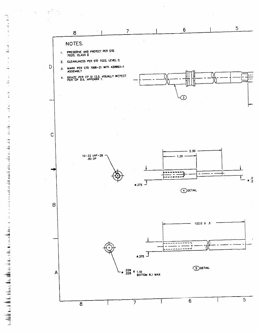
s I 7 I 6 I 5

: NOTES._=

-- I. PRESERVEAN0 PROllE:CTPER STO_ 7020, CLASS Z

2. C_:_oa_UNE:SS_:R Sm 70ZZ.L_r_C¢

_ 0 ,3. MARK PER Sm 7006-21 WITH 42g_33-!ASSffMSLY

LPER CP g.6, APPEN01Xh

.2

= C

-- 10-._20Nr-2e ....... 2JO 1

: _:-__:.__--

B

_- "-'---'------_ 122.0 ± .5 -

•22g _OE:TAILA • .228 ¥ 1.1060TTOM R.! MAX

L8 I 7 I 6 i 5

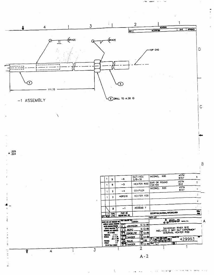
I;,l,lh ,il61Hli,til ,,,I ,, ,_,_

'l' 4 I 3 ii 2 I 1.t-vi _ 1oer.=.,'_ _i12] =_ j,,,_,_

J , ,/

, ,/ , ,t,, ' /-ro,:, r..No D

/

--: 111.7_

-1 ASSEMBLY , '-t.._tu. To_a ,o

C' \

" NUT-HEX INC_EL 600 " - " ASi'M ' --I 3 -6 3/8-16 8167 t

I =J -5 HEATER ROD BAR OR ROUN0 ASTM ,COP,)ER B¢2

,, _ ,., __

I =J -4 COUPLER INCONEL 600 ASTM8167-= 11._...,,:._.:_.__.:......... _ ,, ...... _ ,, __

- 1 3 4,ot,016 il HEt,'ri_:_R0o'4 < L................... i_ ,-.-

4

_ _ . .... _-,-,r,_,_., II - I ASS_UB,. Y

I,l& _'r .... "-i.iild elk 2_G -.- A42_Jg4.

= mml t E OER__ g-t/-_ SAVANNAH RIVER SITE

JmiJ m t_ __r _ INTERNAL HEATER ROO=,=ii .).._TJu_l_tt_l_ ..... '

Jo._ _l /. :_.Fm_-_i _ 42999_ ,:tr

- i 4 I ; 2 1 1

A-2

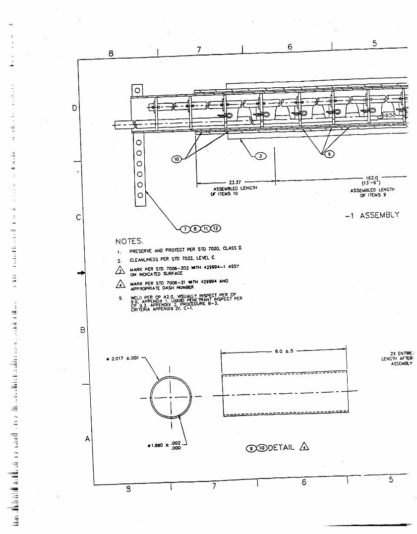
8 I 7 I .... 6 I=m

,.,,, , ,,._ ..... _'i,':-r::".'_: _. _: " : : -,": -:'".':_ ::.._'-'_,'.',,-> :. :". :'. I' ":::_ : _: • " -

°. I

elO l - 2_.37 ...... _ozo

ASSEMBLED LENGTH (I 3'-6")

- _TEM$ 10 ASSEMBLED LENGTH

_. OF' ITEMS 9_

C= -1 ASSEMBLY

--

_

NOTES.- 1. PRESERVE AND PROTECT PER SE) 7020, CLASS 1_

- 2. CLEANLINESS PER $TO 7022, LEVEL C

Z_ UARK PER $1_ 7006-202 WITH 429gg4-I ASSY_-" ON INDICATED _URFACE

= Z_ MARl< PFR $TO 7008-21 WI11-1429994APPROPRIATE OA._-i NUMI_ER

5. '_U) PER CP A2.0 VISUALLY INSPECT linER CP9.6, APPENDIX 1, EIQUtO I_ENETRANT INS,oF.CT PER

: CP 9.3. APPL_N_X ._. PROCEDURE B-,3oCRITERIA APPENDIX IV, C-I.

: B

=

_

--_ 2X EN TIRE_LENGTH AFTER1

ASSEMBILYI

2 _

_ A

: .ooo _DETAIL /_

= 3 I 7 I 6 I 5

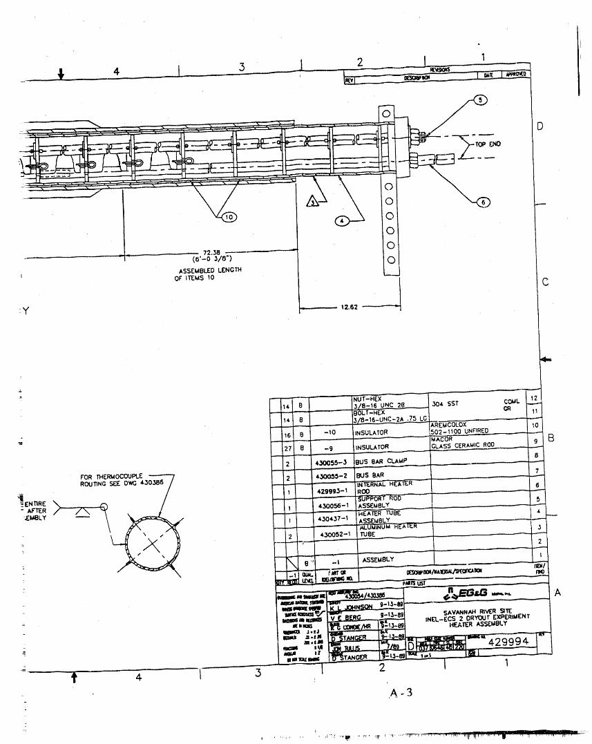
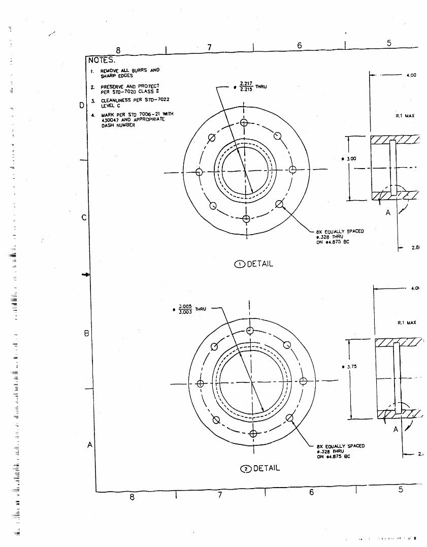
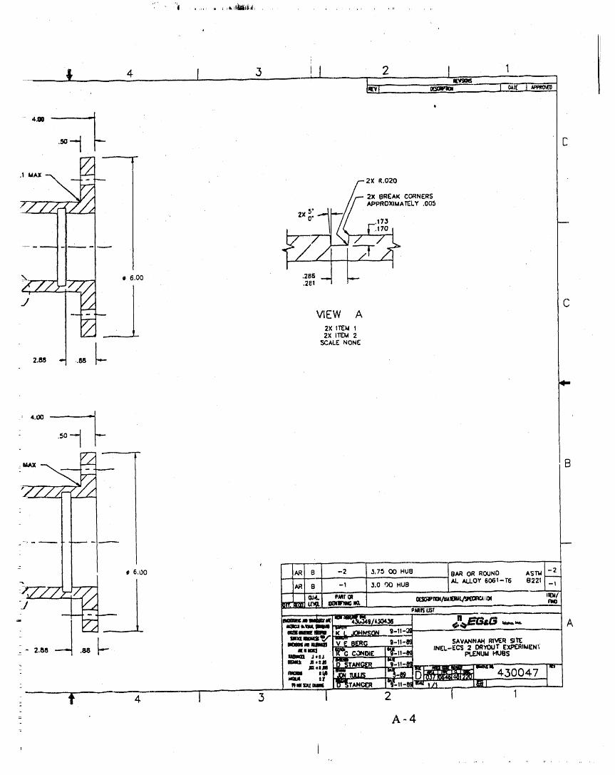
'<" "i .......... i ,lliiii,l_;,ill_..................

,i

-- _ .... 4 I 3 .. !_l 2 I 1

t

- ,li .'_

,.1 MAX - "-- /--2X R.020/IF- 2X EIREAK CORNERS

//APPROXIMATI_LY .ees

,i .173 _

4---- -- ,i_ 7-

z{.%'72'_ _ .6.00 ._._--. ,2_I

- ViEW A2X I_ 12X II"EI_2

I t SCALE NoNE

2.88 "" ..88 _-c

i,,,

' i

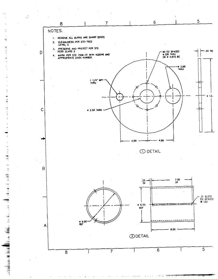
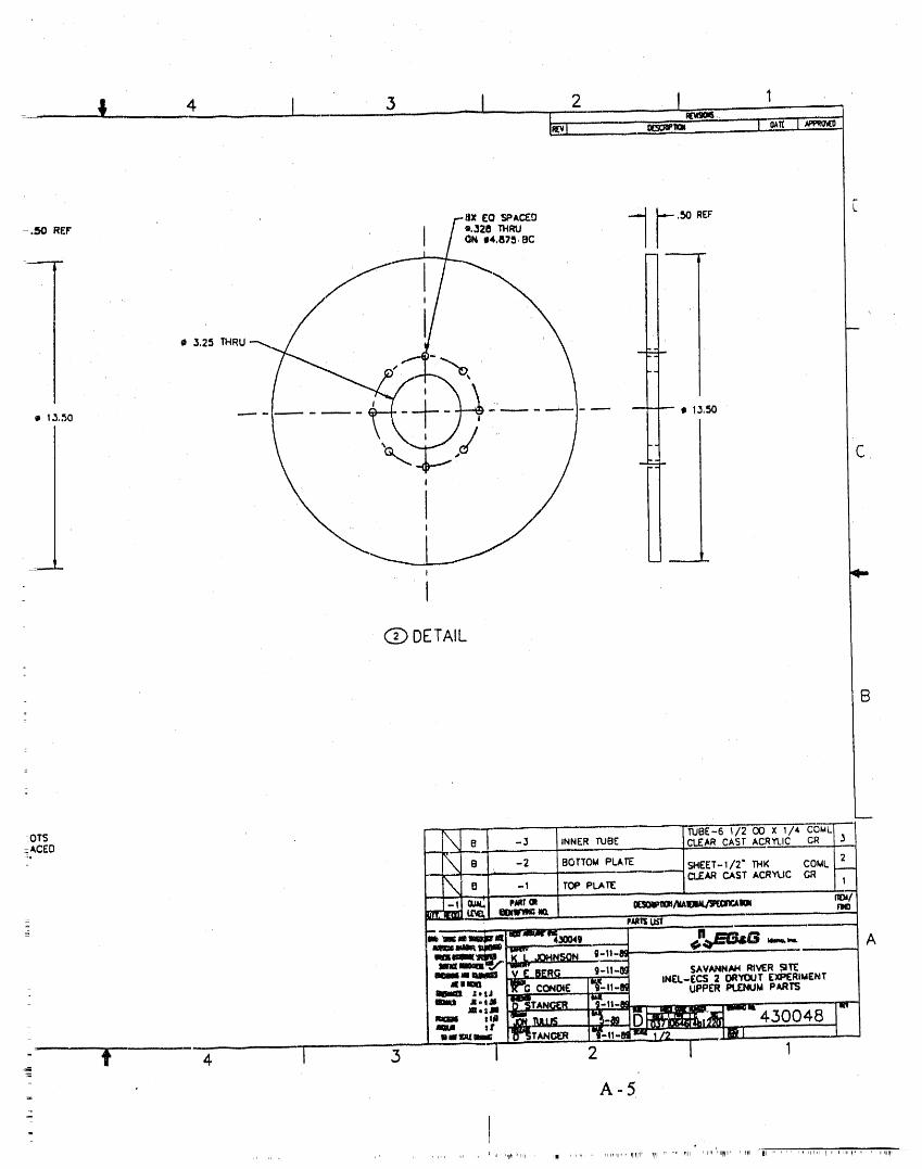
C) DETAIL

o B

w

:OTS _ TUBE-6 _/2 O0 x _/4 c6_Ei "#_.ACED e -3 INNER TUBE CLEAR CAST ACRYLIC GR |3

: -2 BOTTOMPLATE 5HEET'I/2 ° THK COML[ 2

/

-1 TOP PLAn_ CL£AR CAST ACRYUC GR= Ixxm_ _ o_o_p_,/__lcl rm

,,m,,a_uW,mr,-,_- _ _,,-l_-_(il Ammu,u_aIKt._aO_4NSONg-"-mm,_,umm'.,"l'Wu_-__ g-11-m SAV_IN_ RIVERSI1_,v__BE._.... ,N(L-_CS20,,_T(_.,.,ENT

_.tJ UPP(R I_ENUM P,_RI'_

_ ,,"_' _i_ .....4,30048

t 4 i ,3 I 2 1 1

- .A-5

I _' "I_ I,ii,h , 11,I_'II._ ml_irr'iiiii, ii¢ _ii 'I"]Ii"ll_ll''Iii¢,Ii ,, , ,,i,,,,llrq rlI, llllllqr " ' llqll'B'

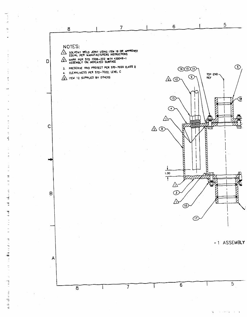
r

I

- II

" I- j '

1,00

_: e / ,I

I

: - IN

- 1 ASSEMBLY

A

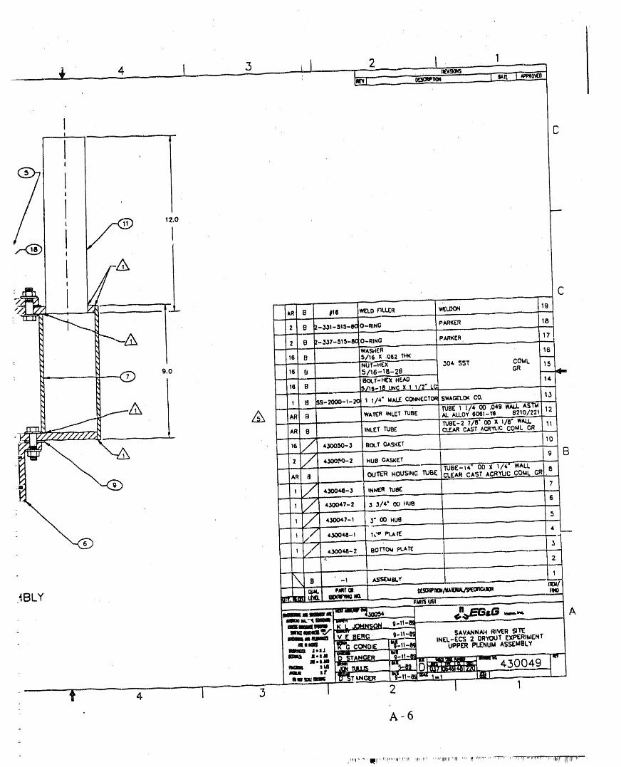
..... + __ 4 .... I, 3 __1 2 I

I

I

! 'j tz,o

- 18,2 |-- 337- 5!5-8(::'O-RING PARKER

WA_-ff....... -"---: i6 ;_,I_6x ,oez_K _

i/+UP;,HCX-- : 30'+ SST COML 1_9.0

- _._, 16 !5/16-18-2B GR

I m i ii_._-_r._ ...... 4,-

1/Zl L(_I

r _ AR+ _ - ..... """ "_, ,| AL ALLOY6,,061-111 B210/Z21 , I_INLETTUeE I _OE-2 7/0" oo x _/8" WALLARi B I

- | _ARc_; ^c._-'CCOm.G_.__;

2 t 4,3OO_-2 HUBGASKET 9 B._- i . ,=---- . .

i 3 314'" O_ HUI_

,! ,_,-, ,.oo.o, +I t 4_4_-t TCo _t_rE 4 --

t ! ,.43OO_-2 8OT'rOluPLATE 3i '

]

IBLY _ -' '_="_Y

- _-_Il'l US!

.l_ _G CONDIE _-_ INEL-ECS 2 DRYOUTEXPERIMENT Imm=B _.=a UPPERPt.E,,NUMAJSSEMBLY I

___.__.__JT N -11-

""" I..... _ "'=_='= _ i_2!_'m=",I=I........ i li_l _ _ ----L_J

'F + I-- _ I 2 1 +

A 6

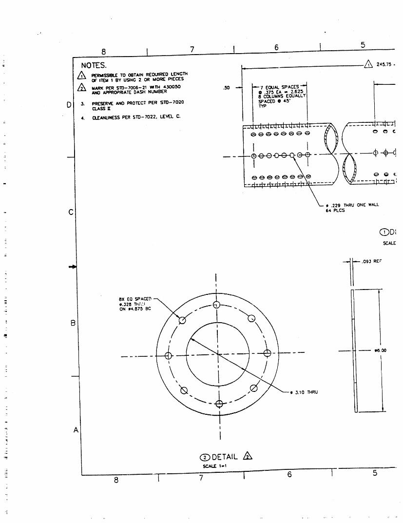
• h,

8 I 7 ! 6 I 5

" NOTES. -- Z'__s.7_A I_"I_gSS_ TO 0eTAIN REQUIRED LENGTH

: OF |TEM ! BY USING 2 OR MOR_ PIECES

! O 375 EA - 2.625 I

O _- _'SCRVE_ _orccrPERSrO-7020 (._.

4. CLEANLII_SS FER 5TD-7022. LEV/L C.

eeeeoeee u ' o oR

Ieeeeeee\e k# o _

= C I).229 TMRU ONE: WALL64 PLCS

: CDD_- SCAL£=

- _ "_ F .093 RE;'i

ON 14.875 BC "_"_ .,.

...... qD6.1_

P

_ A"I

=

CD DETAIL Z__ 1-1

8 [ -/ i 6 I 5

-- _ _ [, _,_ ,1

- 7.00. 8 COU.lIN$EOUAI,J.YSPAC£OO 45"T'_

I i -:rtrntr _h- dr ntr Th-drnh-Th,drnh-rt_frlh--I ____L

--.... : ,;,L.'o.<'.2Y'"120 PI.cs C

,TDDETAIL Z__ 2/_

'- .093 REF"= _7 I B

" BO,.T'GASKEf ..........

8 -2 SIL|CON...._(RUBER

@DETAIL Z_ \ _, [_ _ow_._ i_i.',',C_A_meE _ 'SCAL( 2P ' pjl' al ......... _/IA_B noJ/

'_ I_*'- ""_

_. ,_,,_ _"..._..6-. A- i-ill SAViltitilt@lRIVERSII'E

a lIBi VL_-E _ ii: [-J IN-_-E:CS 2 DRYOUT [XPI_IM[NT

-_'_,, i__ _ ....!_'-"----_, _ _c,,,_Ro.oi ,l,lm, |'_""S'l",llil!GtOItI, t-I!_1:

""'_,..i_"......,,. I_'_jBIttGIlIxi;_.43oo5o".=-..'"jn._,t'="- l'r-,,_ "°'_1 iii,,:: i{ 4 I _ -I 2

A-?

,, , _!, ,,..,.i:....,,#. , . ....,;:;u._Vr _..' ,H ' ' ,.. ,, . ... ,,,,,

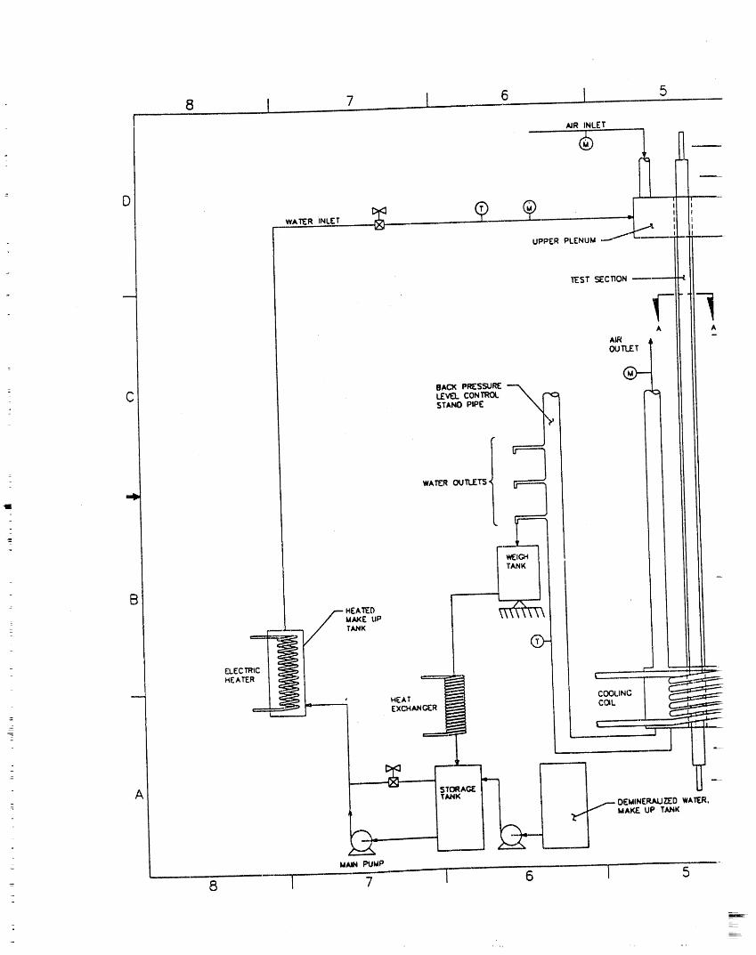
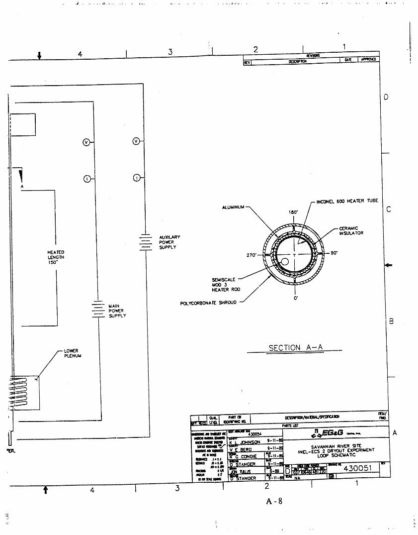
2 I 1 .1...... ,t 4. I 3 ! __ _ i,

=

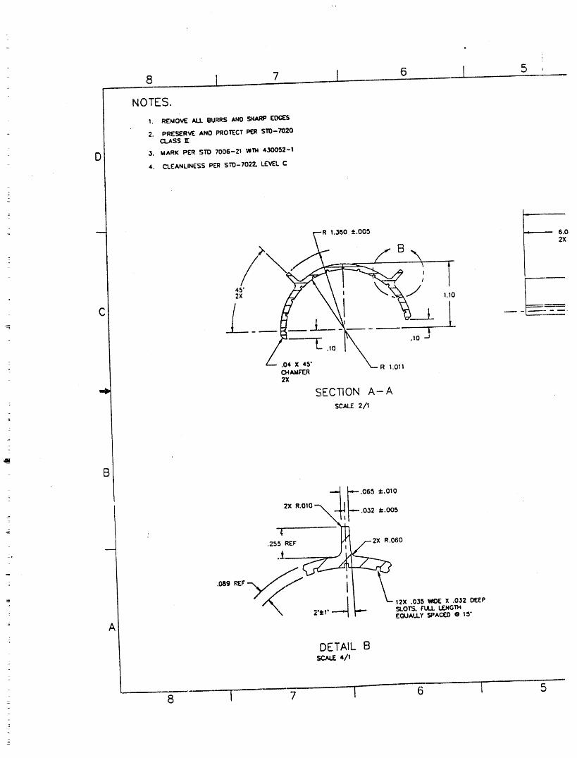
: 8 I 7 I 6 1 5 ,

NOTES.

1, _MOV1E ALL IBURRSM0 ¢_ EOGE'_

2, PR_RV_ ANO PROTECT_ ST0-7020CLASS ]_

D 3. MARK PER ¢_TD7006-21 W11,1430052-1

4. CLEANLINESSPER $I"D-7022. LEVELC

'R 1.360 :I:.005 --------- 6.C2xR

",/I"

1.10

2 _"R 1011CHAMFER2x

"lP: SECTION A--A

SCALE2/11

=

"411

: B

= 2X R,Ol0 _'_.! ''_'" .032 ::1:.005

_' , ,, , ,, ,¢_ _ .255 REF

_'_,1 _' -- _0_ _ _'_

DETAIL BSr.JClE4/1

_

8 [ 7 1 6 I 5

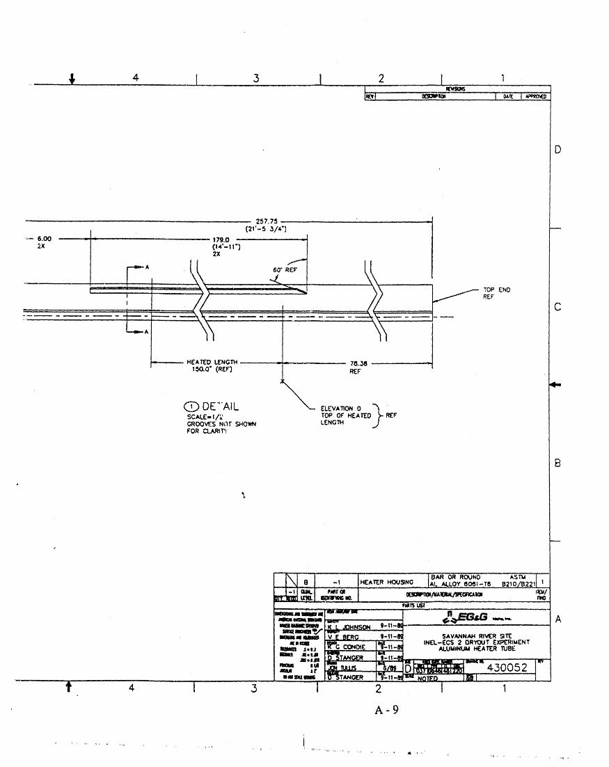
D

257,75 --i

(21'-._.,.,/4"): 179.0 "LI

-- s.oo '-lr)

" ,,r i / TOP END

_/ _ C

-,,..--------- HEATED LENGTH :- _ .... 78.38 _itSO.O" (REF} REF

@ DE'_'AIL ELEV.nO.o "%

sc,,,u_-,/_ TOPor HE,,,_o.j_ ._GROOVE.SN,C)TSHOWN LENGTHFOR CLARITY

.... IeAROR ROUNO AST_ ('

_ ,, "_ -1 HEAER HOUSING IAI,..ALL--.--O,Y.i50_1-/6 . B210/_B221[ lP_r ai ocsow_/_ m_'m'r.a IcM1oonp'm_lm.

Pkql_LIST

' "'" _._=e,G_m_mlmm__- --, _ AI_ilimtmll < L JOHN.SgN 9-I!,-IKIli_l_lB_ ---_ SAVANNAHRIV(R ,'lE

t"C _0,E-*1_-',;'-"; INIEL-(CS 2 DRYOUT[XPERIMFNT4,tj ALUMINUMHEAER TUBE

,U.IJ BrL _ li_¢, B.

-, ,r "_- 3_ 4-30052

t 4. I 3 2 I 1

A-9

i, ,r ..... rm q .... ,, lr ,_' I .

rlt

f

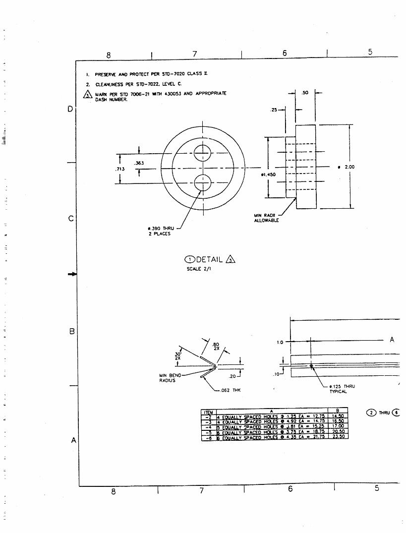
8 I 7 I 6 ] 5

I. PI_SERVE ANOPROTECTPlDRST0-7020 C.4_SS ][.

2. CLF'ANLINE:_'_PER 510-_22. LEVELC.

Z_ MARK PERSTO 7006-21 _MTH430053 AND APPROPRIATE ...DI .50 J.---

DASH NUMBER. [ /D .25 '-- -,,--

[r .... 1-"

t'i ....... ____ ,=.363 '----- • 2.00

•713 t -_et - -

- i

C MIN RADII JJ" "---'--'--" '-

e.390 THRU•' 2 P1J_C[S

-

= (_)DETAIL Z_

= _ SCALE z/_

" ,1.%i-2 J4 [(_./ALLY SPACEDHOLE5 _) 4.25 EA .- 12.75 1I,, -3 14 EQUALLYSPACEDHOt.ES@ 4.g2 EA .= 14.75 ] 16,50 J

_Z.__,I_£OU_LLY SPACED HOt2,_@ 3.7S rA = t8.75 I 20.solA [ -6 16 £0UALLYSPAC£D HOLESO 4.35 EA - 21,75 ] 23,50|

8 1 7 [ 6 I .5

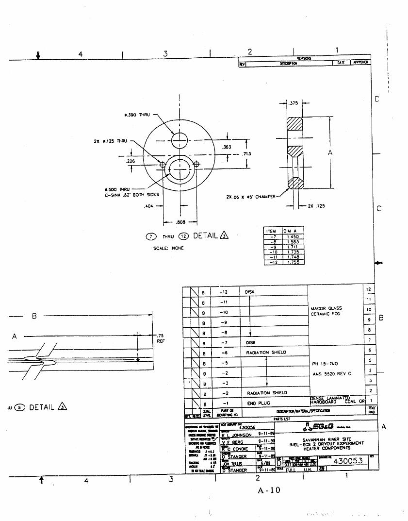
C--4,-.375-,--

_ _..o.q: ]-'1 .125 C

_.,,,,-- .808 --"

@ _u @ DETAILz_ 1-,_:, 0,,4,-7 1.450

_ -e i.583 _SCAL[: NON[. ....-9 1.711

-_o 1,73%_.-I1 1.7,4.8 i

'_B -12 OISK 12

)l'x,Js -_i ii

_1 __ 8 -lO

I B .... -9-,

A _ _ _ _. s -a _ e

/ / _ _ . -7 o,_

_ ,, ,

-: e -2 ,&uS 5520 REV C 2__.

'_ B -3

e -2 RAO4A'nONSi-lIE:LD.-u_'> DETAIL/_ a -1 [-NO_uc c= 1

mmtlm

IiliUa_lliB v.._J_RG g-11-_. SAVANNAHRIVER SITE:,.,, i,_ _J INEL-[C5 20RYOUT (.XF_RIM(NT I

atom ('--C CONOI£ I-9--_ HEATEROOMPO_ENISi .tj II - I_lt

Imu a,,= ) S_'_r.._:_I s-li-_ , -.--,===,_.... m--= ,,_ " -" !%_ 4.30053

_ ,,__a_.-__ 1 ',,=,=_I= .. _I I

..... t 4 I _ iA-lO

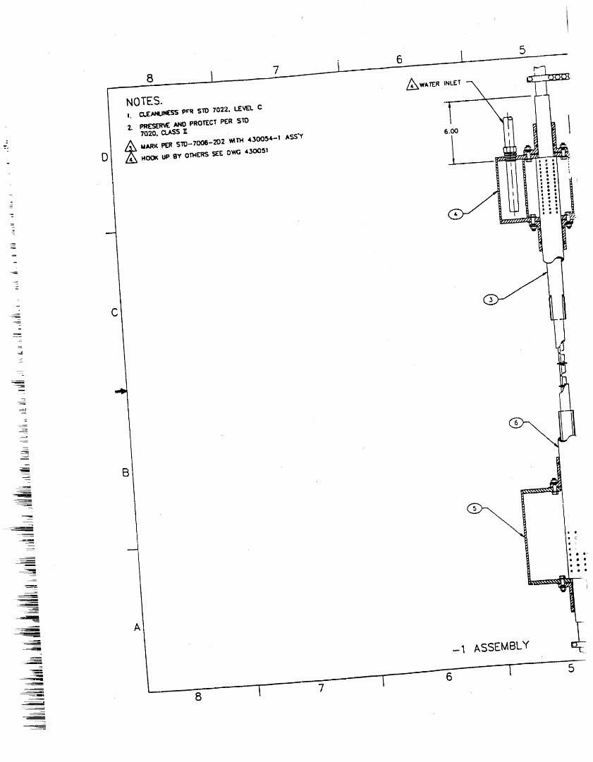
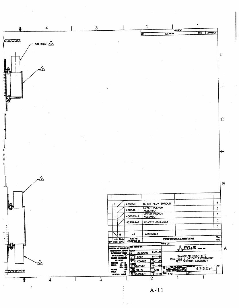
.¢_ 4 I 3 I 2 I

-/I / DI

,mi :

_ -

_ , ) ,, , , , , , ,

1 /t 4_50-1 OUI"ERFLOWSHROUO 6....... LO_R'"'PLENUM ......

1 430436-t ASSEMBLY 5, .......

UPPER PLENUM 4. 1 / 430o49-1 ASS_eLY, ............

, 1 / 429994-1 HEATER ASSEMBLY , 3

PmI5LIS;

J, mL=_ __. G ,._._ Amm__ _ JOHNSON.._ g-,-eKlUmBG_tlMII_B Y E BERG g-ll-_ SAVANNAHRIVERgT_

""= :_C:CON_W¢_ I%'-,,:=,NE_-Ecs2OR_TE_R,_C.TIBm= J,tJ b_ TEST SECTIONAS_MBLY

=*'='-- -'"_,: _"-" 43005_"='_ :_' _.uus ,l ,m•-=,-, '_T,_,=_,, ]"_-,,-='==,/2_ ._, }m"_ ':i

t', 4 I 3 i 2 I

A-11

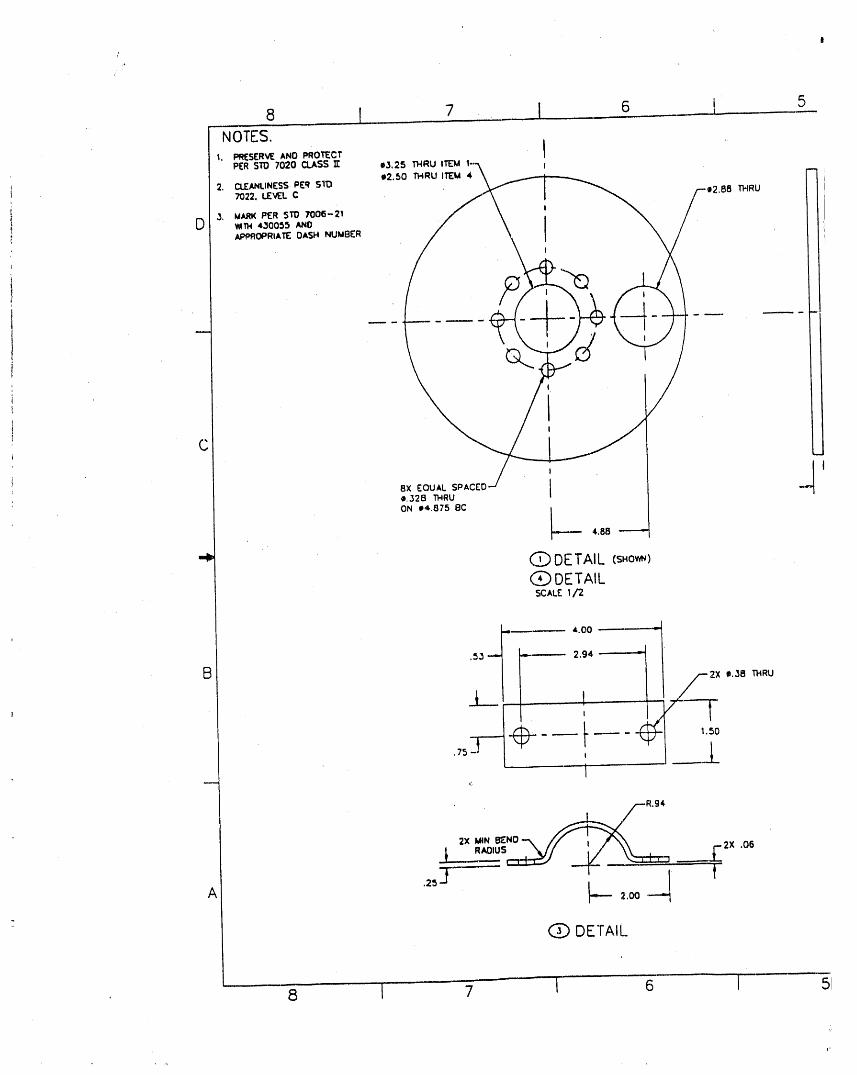
r 8 I 7 ,I 6 i 5NOTES.

PERSID 7020 CLASSII e3,25 THRU ITEM I

I 2. CLEANLINESSPER SltO e2.50 THRU ITEM 4 --, 7022. LEVEL C B8 THRU

i 3, MARKPER 51"0 7006-2,, D .,._ 43005_ AN0 I

APPROPRIATEDASH NUMBER Ii

l

S

i '

' Itl1 !

_ C

8X EOUAL SPACED I' o,328 THRU

ON t4,875 BC

_-- 4.B8 -------"

"_ @DETAIL (sHo_)@DETAILSCALE I/2

.,,. 4.00 .,,.

Be.3g rHRU

.i__.., [1.50

- I

2X ' _R.g4

@ DETAIl_

a I 7 I 6 I 5/

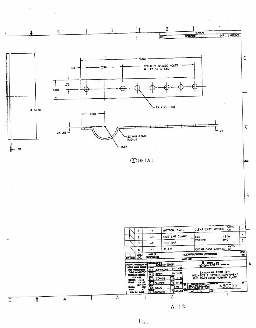
L .... 9.62 _i

.53 z_ ---------------_OUALL¥_ACEOH0_S----------{

f .75

J._ f ,\$ 13,5(] "_--7X $,38 THRU

I _ 2.00 q ,,

' _t _ ..i. -', , i i-, " l't, '_'.... _t, i, c' ' -----}-j, _,..__ "_,--2XMIN BEND

J,I X RADIUSr

(Z)DETAIL

-4 BOTTOM I_.AT_ CLEAR CAST ACRYLIC GR i 4 --

" L i I -3 BUS BAR CLAMP BAR ASTI_• ,.

'\ _J I -2 BUS BAR COPPER B42•

".... I' COM/..!\, a I -i PLA_ C_ cast A_C C_i i j I

P_13

--,,a.. '*_/,_ _"_,G --.. A

ImmRlIImE! _ BERG t-II-,B_ SAVANNAHRIVER SaR""= _o co.oi_I'_;,,:, ,._-Ec_2oR'_,_X_R,,,_N'rI

Illl_ i,=a BUS 8AR,LOWERPLENUMPLATE Ii

I 11/ IIi-- - i

®=_i_ ,_, _,_'__ I'_-_"-_'_ I=,I U.N. I_I ..i- .. - .....[ I

5 t 4 I 3 ..... I 2 I

A-12

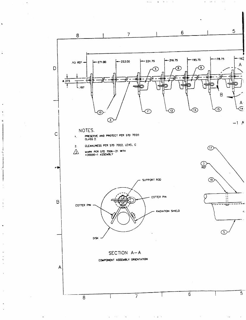
,, ,, L' , , ,

8 J 7 ] 6 I 5

!'_ ._,3 I_EF"..,_ --'"271,00 p25,3,00 "='--231.75 -'-'-216.75 "=-19&75 "=--t78.75Ld

_ ,• _ _

_4

i

i -1 ,_C NOTES.

_ PI_S_RME _O PI;IOECT PER STD 7020Q.ASS

i 2. CLEANUNE'_'SPER STD 7022, LEVEL C

U,_K PER STO 7OOb-21 W_TH] 430056,-_ _SSEuf_.Y •f

1

iiSUoPORT ROQ

COTTER PIN __

RAOIATION SHIELD

SECTION A-A

CO_4PONENT ASSEMBLYORIENTATION

A

8 i 7 I 6 T 5

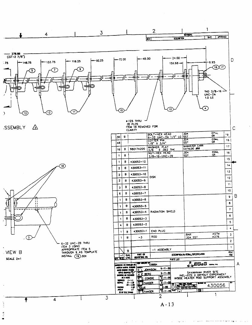
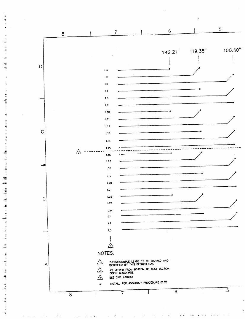
8 I 7 I 6 1 5

__ 142.21" 119.38" 100.50 I

L4. <j /L5

- L7 _.

- /_ _ 1.8

L9=

LIO •

/.L11

- L12C

- L13

- /-

L14.

" L16 • o /J

/==(I= L17

L18

L19 :.

L20

L21 •_

L23 /

= L24

L1 = ,b

_ I..2

_

_

-: NOTES.

- A ,/_ r_RUOC_l=,t.ZuE,OSTOacU,',RKED_oIOENIInEDOY TH_SDE_A19_.

L_ ,_SwEwEO rrROuBOTTO_ OF"TEST S£CTIONGO4NGCLOC_SE.

- L_ SEE Dv_ 4_A)052

4,, INSTALLPER A$cJ;;EWBLYPROCEDUREGI32

:_ 8 I 7 I 6 I ,5

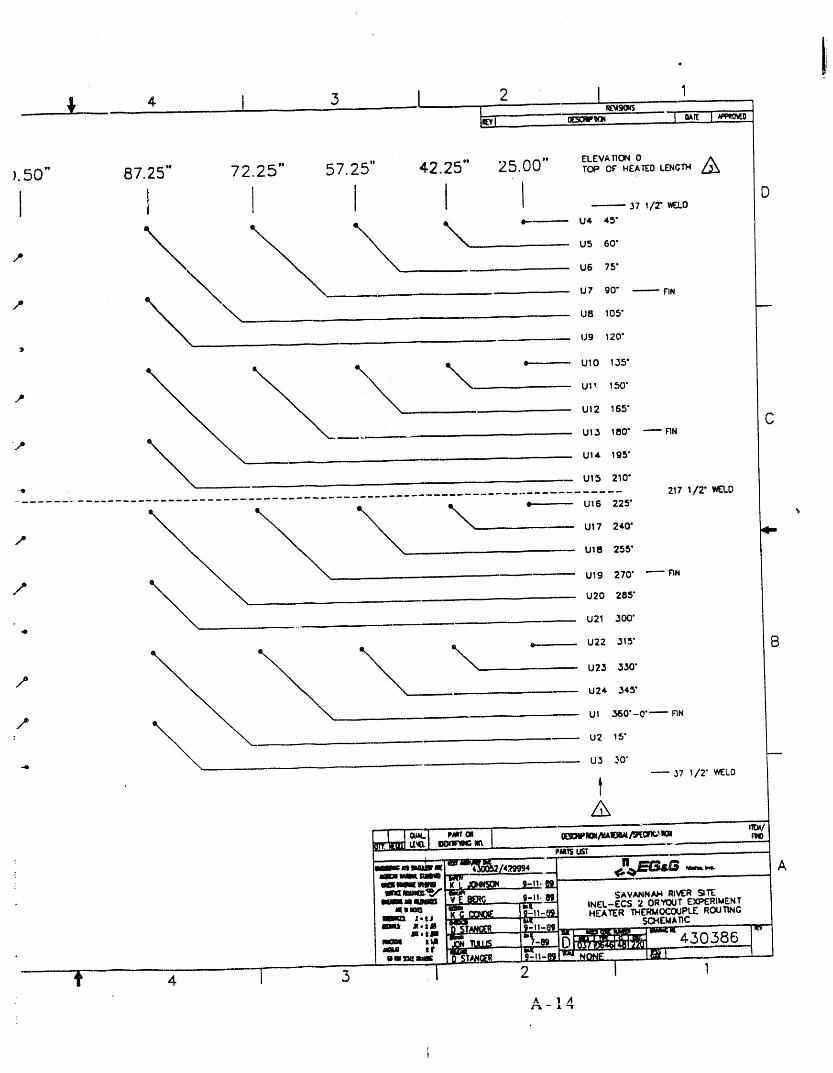
........_ 4 I 3 _ ,2 I I

].50" 87.25" 72.25" 57.25" ¢2.25" 25.00" (LEVA.ON0 /%ToporHE,_oL_om

1 1 111 o-- 37 _/r V_.LD

]1 _ us 60"

t. ._ o,,o. +U8 105"

U9 120"

_ e-------.--. UIO 1,.35°

....... u,2 165"

L,," u,3 ,ao" -- n++ C

U14 195"

-'OUI5 210"

- ---- 217 1/2" _"LD

_ e.-------_ UI6 225"

",,. ,je Ul 7 24.0' @"

..... U18 255"

-_'P U19 270" -- IaN

U20 285"

,di __U21 300"

/ _', u2_ ._..,o"

__,x_ - U24 ,3¢5"

Ul ..,_50"-0"-- nN

U2 15"-41

U3 30'

37 1/2' WELD

tr --- , i t ,

r I tom.I ,,,,ro, I ,m,/+ , , PMfS

-- ,,,mm,,,,mm.m,m ,,_ -- ------ _'_ A

nimlm, lllm t [_BD_ 9-It,,8,D SAV/_N,a,b,lRIVERSITE=Imma_; mm --T_F-- INE'L-EC$ 2 DRYOUTEXPERIMENT

J.t& ( G _00NIOF. 19--!1-_, HEATER THERMOCOUPL_ROUI'_NGJ - I,IB _ - + 11_1=.,,, L._.L_ so.c(M,,c

,,m.._ _LLe; I _-e_. 430,IIEIlLI IT l_I + ,,_..... "==,,-,.,, __ . l,,,,-m_"_om-,++""--,-1_t _

4 l 3 I 2 i 1

: k 1 ,4

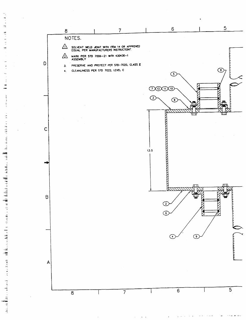
- 8 I 7 ! 6 I 5: NOTES.

Z_ 5OLVENT WELD JOINT _ITH ITEM 14 OR APPROVED

EOUAL P[R MANUFACTURERS INSTRUCTION_ __

_ 'MARK PER 5TD 7006-21 _TH 4304,,_6-1 It= ASSEMBLY

D ,3. PRESERVE AND PROTECT PER 5T0-7020, CLA_ .E

_ 4. CLEANLINESS, PER $10 7022, LEVEL C III

_

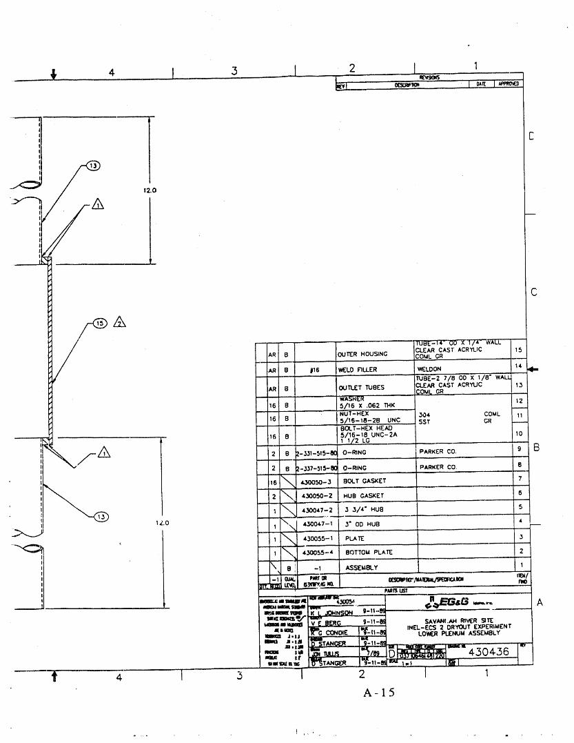
C

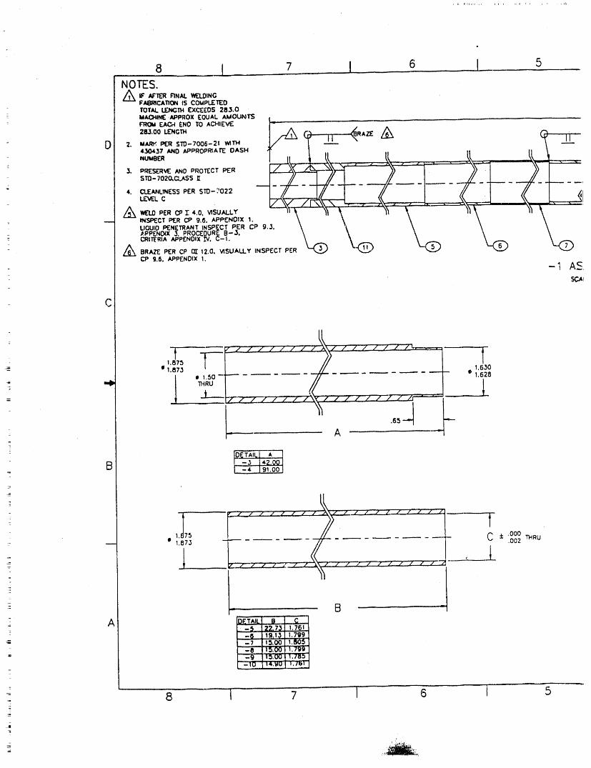
8 I 7 i 6 I 5NOTES,

,o,__:r. exceeds2,,._.o,.,,o,,,E,_,.,o_COU,,L,_,OU,.,=,

J/ --

430437 /_10 AI:)PROPRqATEDASH _ t

_._, I_j_ i IL.___ .... IL ..... li _ .....

'- _,o-,o,o._ __I_J___L//J_ ._J/ -I ---g:-J-----//-L--_4. CLEANLINESSPER STD-?022 I // I // ! il _ I! I I! "T--- ---r

..... ,L7_wzgz ....... . L=jZ_ _I_..0 PER CII Z 4,0, VISUALLY: -- INSF_CT i_R CP 9.6, APPENDIX 1. \ \ \ \ \

LIQUIDI_NEI"RANT INSPECT PER CP g.3 \ _ \ \ \= ._.PPENOIX3 PROCEDUREB-3, ' \ \ \ \ \

CRIT_'RIA AP'PENDIX IV, C-1,

- A BRAZE: PER CP _ 12.0, VISUALLY INSPECT PE

o,9.6.,,_PEND,xI.- 1 Ac:

C

: L-- li 1,873 '- C :t:: .000,002 THRU

-- B ....., __ ,,.

L::-_:l,s.oo11._os1

=

= 8 1 7 I 6 I 5

_ ,

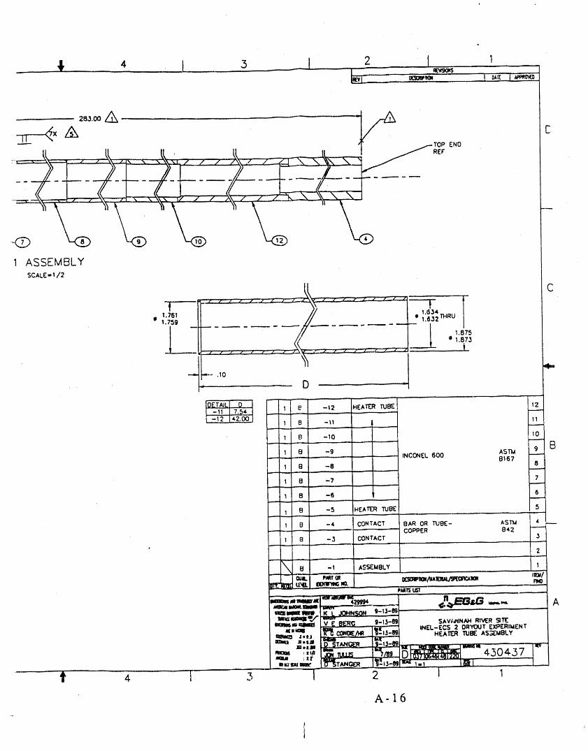
u

L

__.____1,_ -_,, I_............ [I,_, 2 ,, _[1_, ...... JL_ ] __. E,o

1 ASSEMBLYSCALE- 112

' ,::- II // ' ! ',:_i_,..oL:F-.T.-Z: Z:::IIT_L' ' D

T_I e -,2 EHEATERTUG I..Z__ZI B -_, I 11

1 El -g 9 B"--'-_------ . ,. ---. : " - INCONEL 600 ASTM

1 B -8 B167 8

1 B -7 7

l B -6 6--_. _ _

1 B -5 HEAI"E'RTUBE 5,, --..

1 B -4 CONTACT BAR OR TUBE- ASTM 4 --........ COPPER B4 2 --

1 8 -3 CONTACT 3

2

El - 1 A.C,_MBLY.. _ _ o(Ii_ t_1_w./,J_r_Im nwo....

_,,,.,_m,. _ .,...*L'__ ------- """ A,,=,,,,-mm ,._L,_.__NSO,_9-13z_!_me,,,= =cram

=lm..... _"-:-_ '"i_i- _ I INEL-ECS 2 DRYOUTEXPERIMENT IJ_lJ

m_s_ _ - Id',_ "-1 L_ ' _ .... _'_ l

•-,, ,=, __ _--.-I_q.D_ , ¢.50¢__7/1,=,=_==,_ D-STAN_ : l_:_s.:.,,_l_ _.1 I_ 1 " - ] .....I

t ¢ f 5 - 2 ) 1

A-16

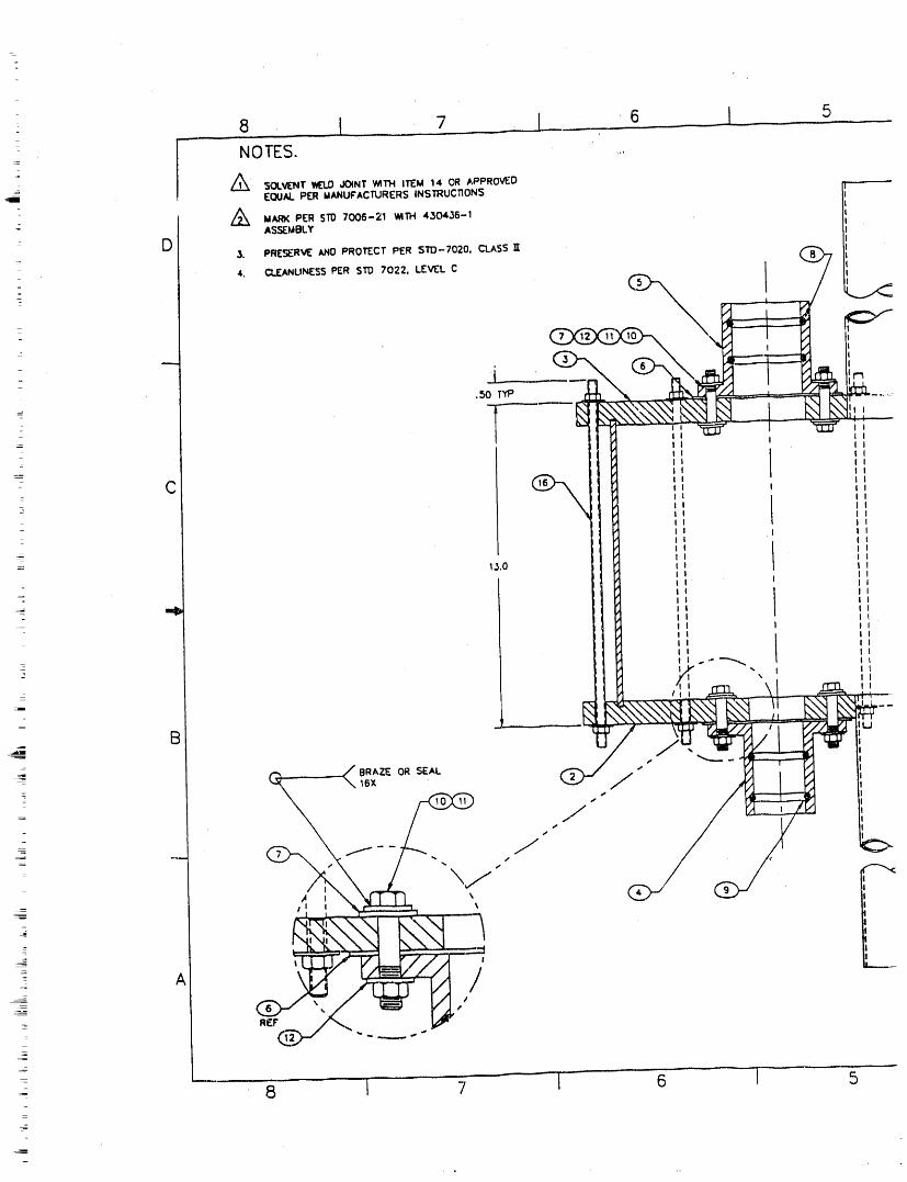
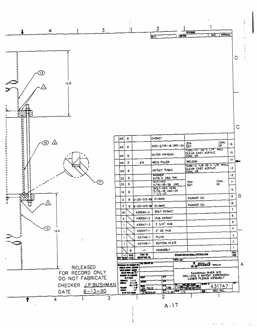
D

12,0

it -! p

! ,

I,0 '

I , Cd !

la I_ Ju_ B GASKET

rt ._0'i COMLtt AR B R00-5/16-18 UNC-2A EST 16fl Iq _ _ ............. GRzl s_"l'_ " _JBE.-16-' DO X'I/4- WALL --

_l I _._ AR B OUTER HOUSING CLEAR CAST ACRYLIC 1,5

', ,4, _=- , ........ comk c_.....tl

. , "rueE-Z 7/8 0'0 x i/8" WALL

. ] AR B OUTLET TUBES CLEAR CAST ACRYLIC 13" ...... qOML(__IJ I " " WA'_HER _ ....I_ 12_= I I / __.132 B 5/16 X .O62 11.1K

I .. NUT--HEX .......tt 132 B 304. C0ML 11

, __.=i,.'._p/ ,_ __ _/,6-te-ze UNC SST Ge

J___ BOLT-HEX H-_AD -"--

,_ tX_ - '16 B 5/16-18 UNC-2A--- __ ,, _,_I_L,C .... lo# _ _ 2 e Z-331-515-60 O-RING PARKER CO. 9 E_

, , , ,. ....... ----

__ 2 B 2-337-515-1_10 O-RING PARKER CO. 8,, _ ,, , .... ,, , ,, _ ,, _

is _ 43ooso-3 BOLTGASKET 7, . _ .... , _ , _

___ 1 4,._047-2 .3 3/4" HUB 5

,=.o .............430047-1 3" O0 HUB 4

, 43174B-1 PLATE 3.... _

43174_B- 1 BOTTOM PLATE 2

\ e -1 ASSEMBLY 1

_ai_ ust .............

...... ..... ' RELEASED "="'"=='_ "=='_= .............n==_.FOR RECORD ONLY ,Btu, w= ..............DO NOT FABRICATE "_'""="_ _

J,=J .... LO_ER PLENUM ASSEMBLY

CHECKER .J.P.BUSHMAN m ,.., _= =,-

..... - -- -- """ " IDATE 6-13-90 _, ,':t _ "" 4_[31747 "_-4 T _ I 2 I 1

A.,17

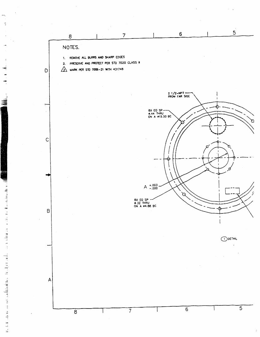
8 I 7 I 6 J 5_____NOTES.

1, REMOVE ALL BURRS AND SNARF j EDGES

8X EO SP0.44 THRU .,ON A $15,50 BC

C i

i

//////

_ /

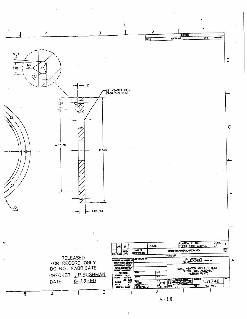
' Z B7 ="

..... i._- ,-_K _L I ---c.l,k'_ ..... line-- , ,,,

RELEASED .,n_"FOR RECORD ONLY _,_,.,._,,_ __ "--,"- ADO NOT FABRICATE _,m_

Imo_Ig_MIII OUAL.HEAT¢'OANNULUST_$T-

ml,,m_lI am i_i - " OUTERFUEl. A$SEMBL.Y

CHECKER _.P,BUSHMAN _ _''"'" '==-- : 1""--- P=,uu _.,,,r_DATE _ _ ,_ ,,,,.....

,'_ ,r - DF_;i_r_[,]_ 4-31748 1.,,_:_,,___._,_ l_'-"._-_o ,_ct 4 ! ..3 ) ' 2 l 1

A-18

Appendix B

Measurements Lists for the ECS.2 and

ECS-2c Thermal Excursion Experiments

Appendix B

Measurements Lists for the ECS-2 and

ECS-2c Thermal Excursion Experiments

Common practice established during the INEL thermal excursion exper-iments was to use a shorthand notation called the "DAS tag ID" when refer-

ring to a particular measurement. Since this practice was used throughout

the body of this report, reference information regarding the relationship

between the measurement ID, measurement location, and so forth, is pro-vided in this appendix.

Since excursion experiments were conducted in two different facilitieswith different inner heaters and instrumentation, two instrument tables

are provided. Tables B-1 and B-2 apply to experiments conducted in the

ECS-2 and ECS-2b facilities, respectively. Columns in these measurements

lists contain the name used for measurement identification, the tag nameused in the data acquisition system that is associated with the measure-

ment identification, the type of measurement being made, the physical lo-

cation of the measurement in the test section (or on the facility), the test

section fluid subchannel where the measurement is located (if applicable),

and the range over which the measurement was specified to operate. Note

that due to instrument failures or electronics problems, not ali of the

mea_,_rements listed on the attached tables may be available for a

particular experiment. Appendix I provides a list of known problematicinstruments for the excursion tests.

B-1

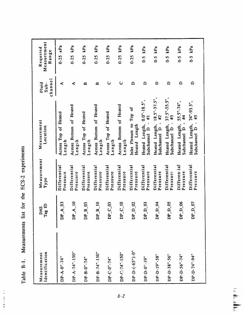
i i i i i i

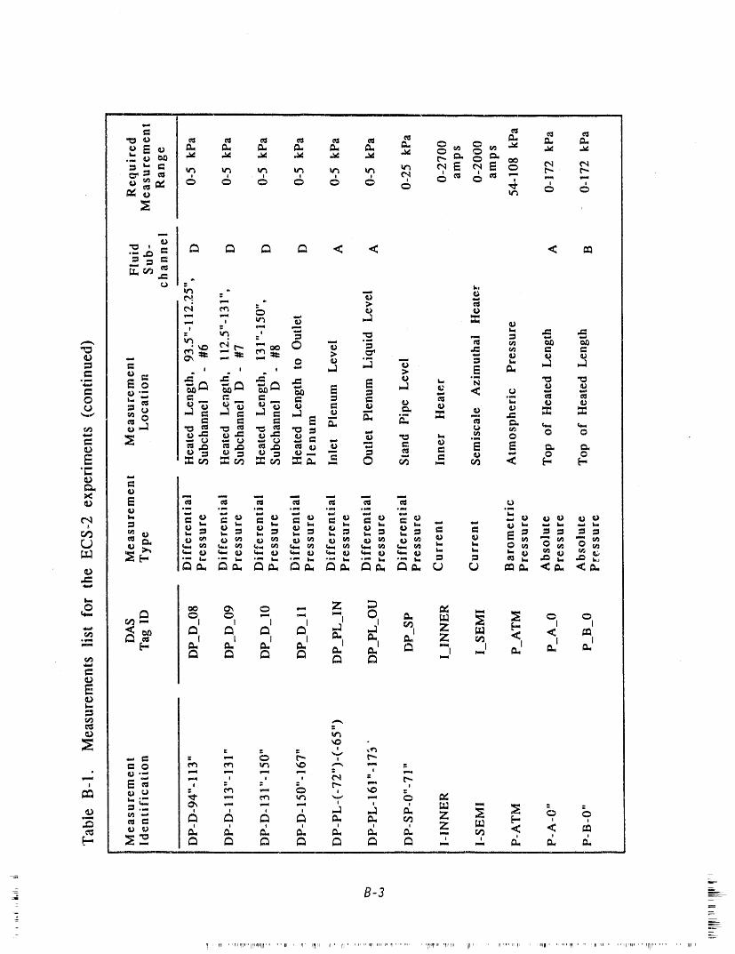
- B-3_

___

___._

I ' _n'' ' '_' '1'II" II1'_'rllt..... IIII ,r ,lr IIIII I} '" II1' , ,r Ii "T''U', " I_ .......... II"llI'l'" Ul I" "111.... II li'' r,,I, ' '"U_I ...... _' ,H ...... li ,, ...... '11'"' ' "rllil ......... Iill i

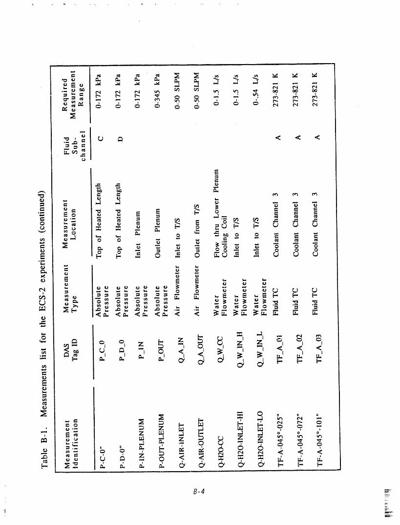
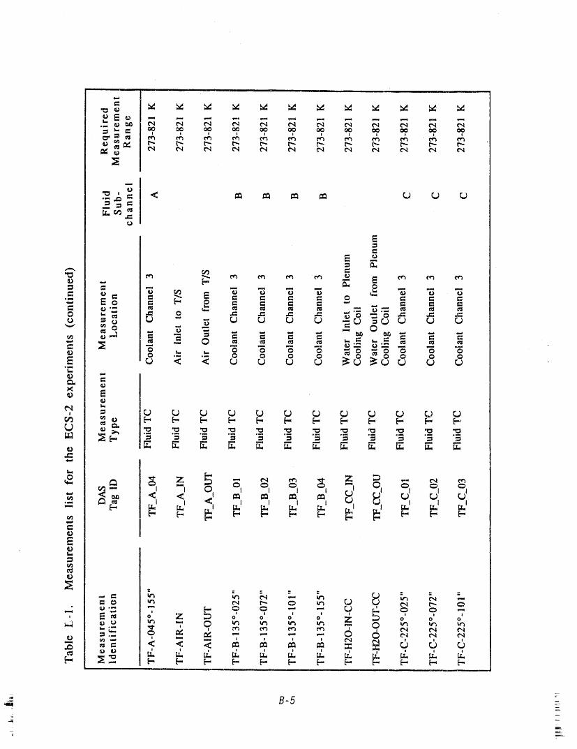
i ii ii ni

I ! I I I ! ! I Im m _ _ _ m m m m m m

N

B-5 -

,,...,

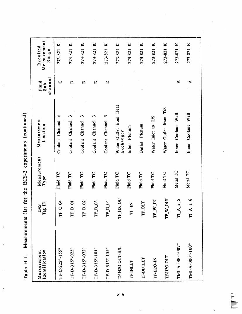
[.T.,O0

o _- .= .= ,= .: .= -o Or.- _., .. 0 0

o o o o o o _._- o _ _ o o

:: r,.) rj rj L) L) _ _ rJ rj r..,) rj rj

,.=:

0

H

:E r-- o

_ _ _"_ o' ' ' ; ' 0 0

=._ e_ m m m m 0 ..1 0 <m

.o _: -, 0 =: =: " "

[-- :_-_ _ E-. E-- E- _ _ E- E.- E- E--

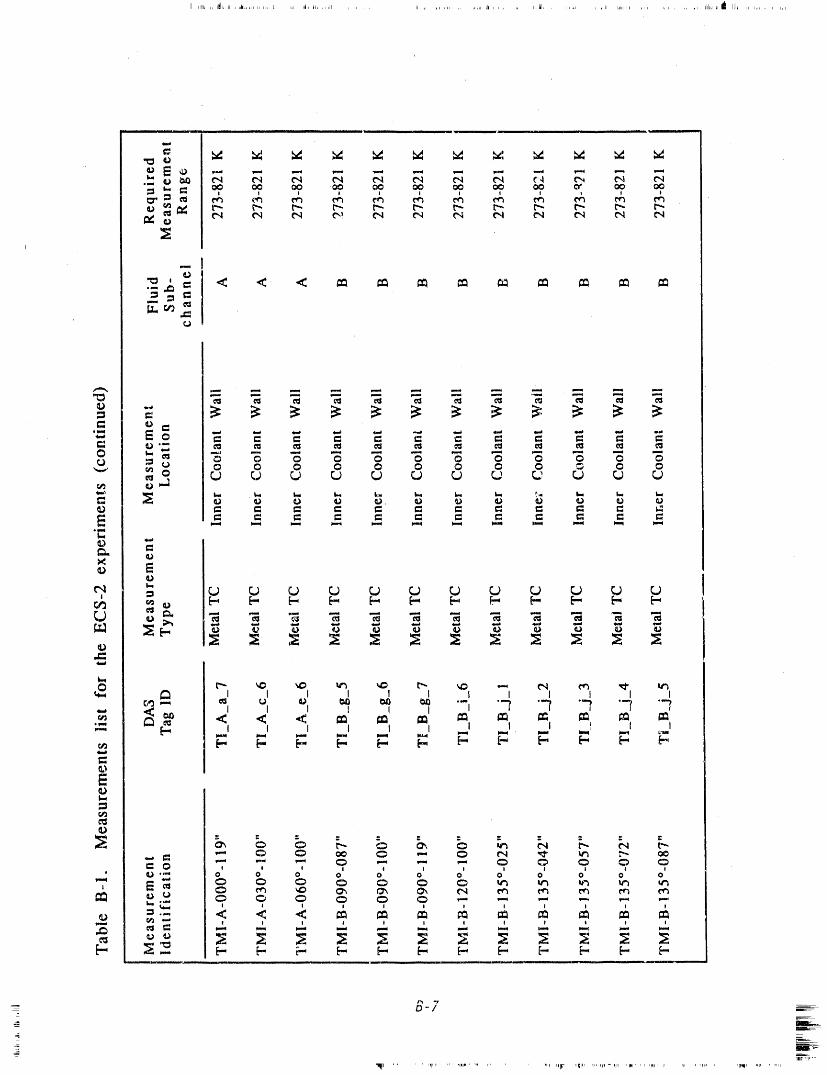
..... mp,,, ii i i , i i iiii ,J_ i iii •

I I ! I t I I I _ I I

_m e_

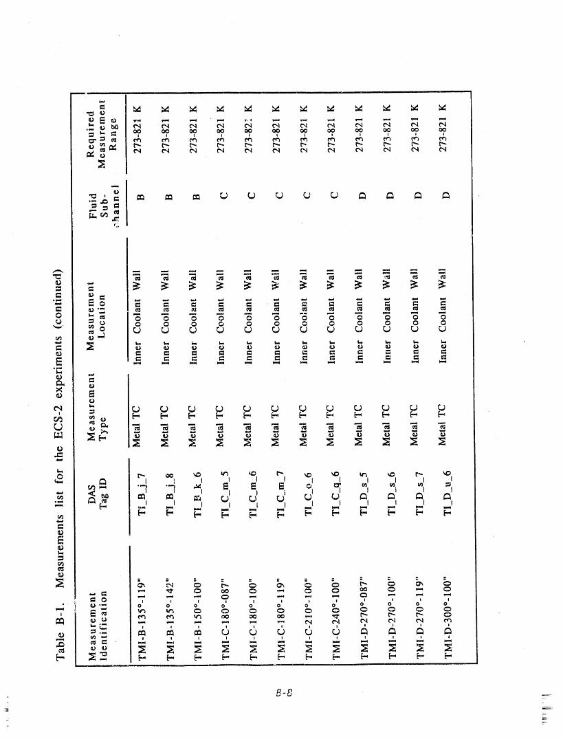
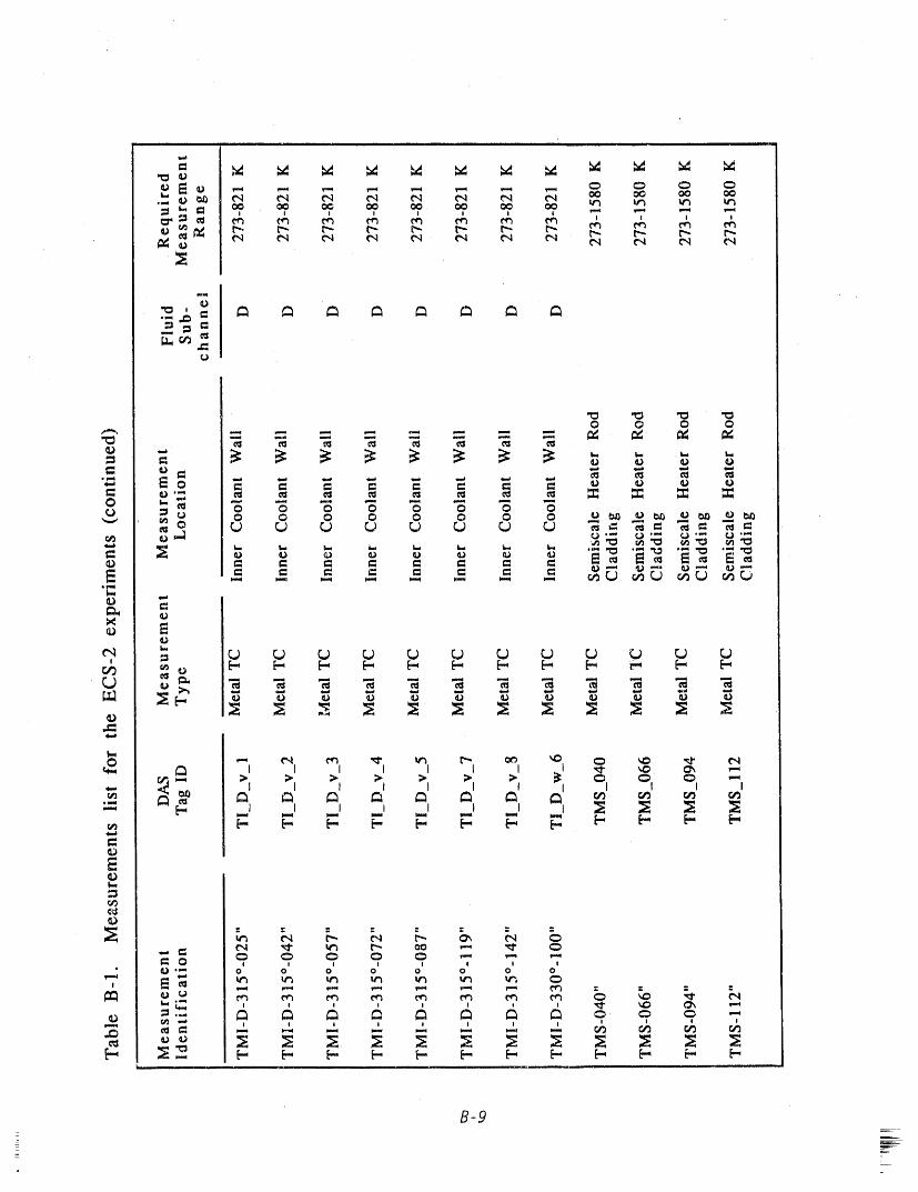
B-9

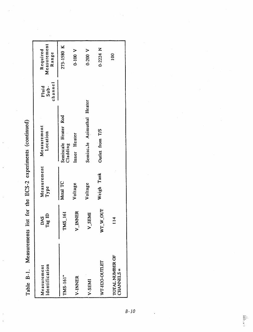
i i ii i i ii lm,li IIImll I II

._o ;> ;> Z

N

B-lO

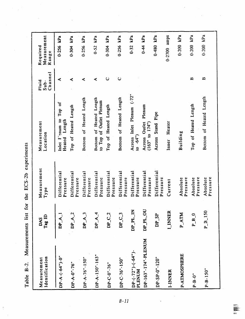
B-11

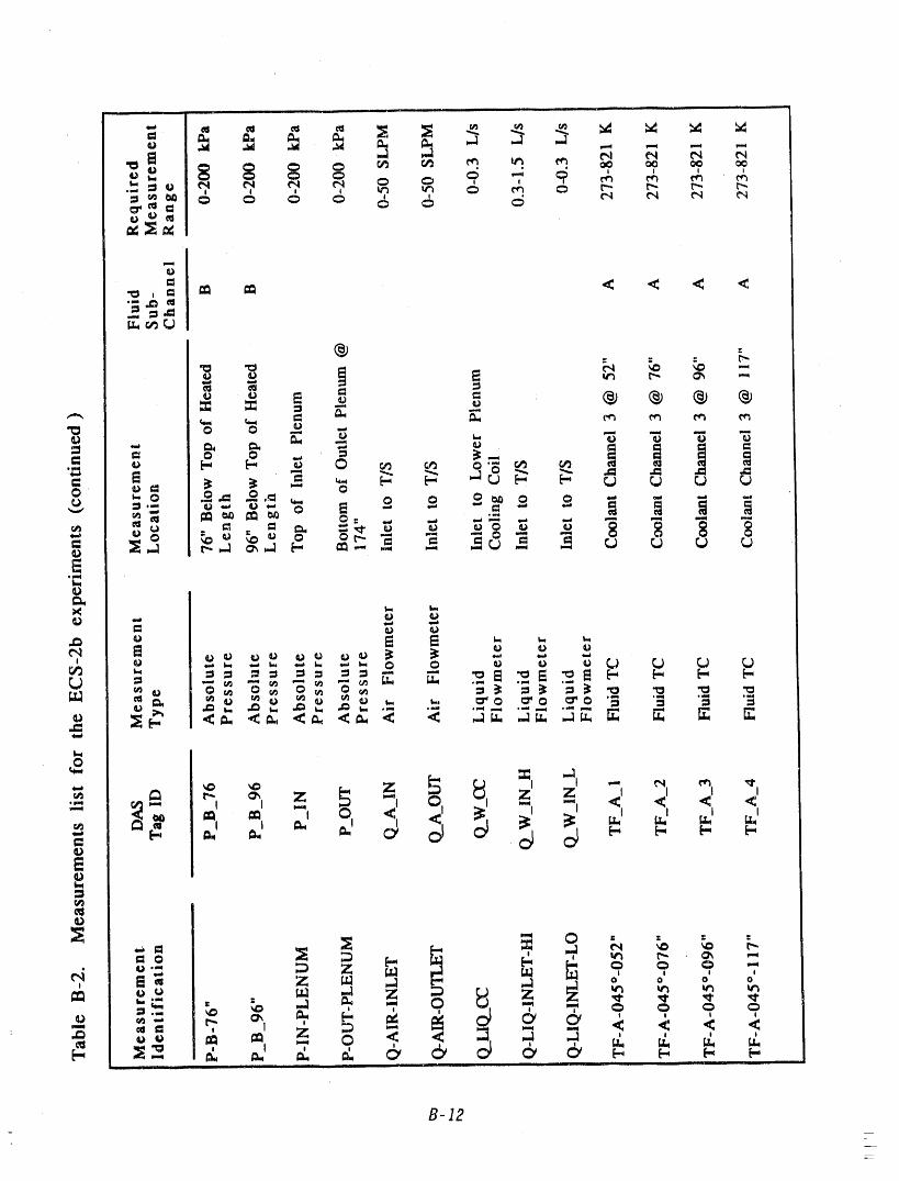
•-- i iii- i

eq e,l _ IN

= < < < <•_ . I= I_I

® = .- K

== _= = = ® ® ® ®_ = --

I= o I= o. _ _

" 1_. _ 0 o -- = = = =

0

1

_ _ _ _ .............

_ I [.i.I I I [,II

r_ _ =l flail _._l l 1_ _:0EI,,i

" 0 =__. = =

o.- ;:::) Z _, o, Q, "T_ Z _ .,.a _ o o o o,

,_. o., =, E- = _ C_ CY ' ' ' ',-- _== , I _ ,- ,- . < < < <

.c:) =o = = Z _- o < _ ,-= _ _

iii!i i i ii i iiiii

B-12

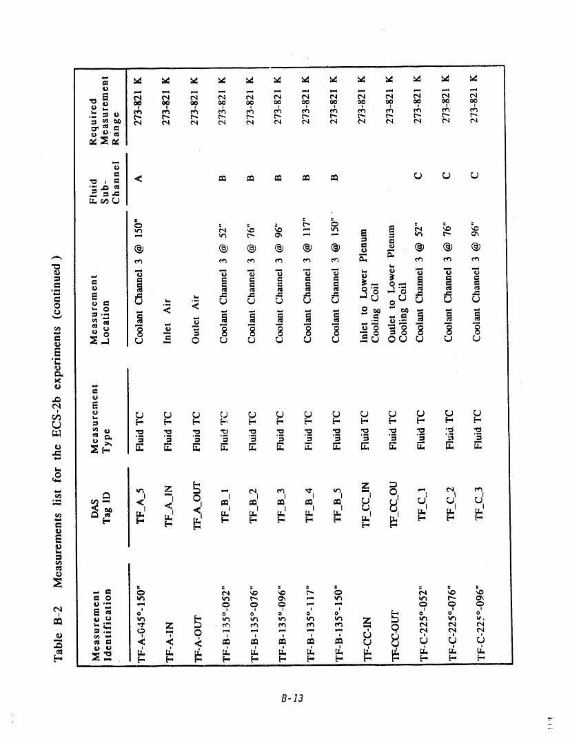
B-13

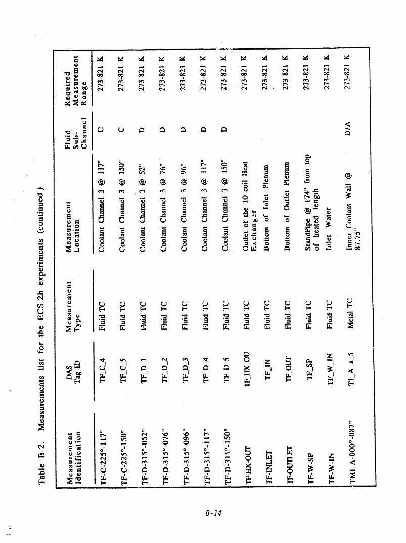
i i i iili 1_''_'_"''_'- ' '

{_I I g I I I I t t I I

_;r -- i,_

B-14

@ ® @ @ ® @ ® @ ® @ @ @ ®

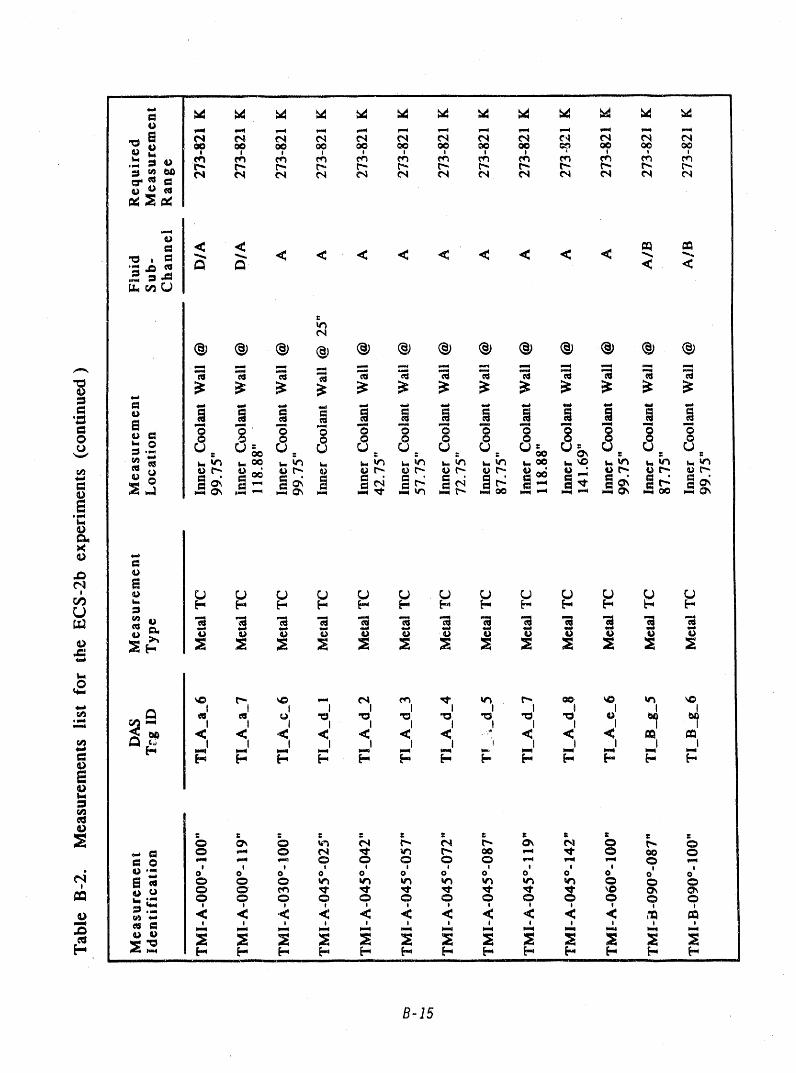
o o - - - - - - - _ _ ? _ ;__

_ N, _ _ _ r_ _ r_ r_ _ _ _ _ _ _ r_r._ _ [.,. [... [.. _ [.., [.. [... [.. [.

'" I I I I I I ? I I

c_ I I I I I I I ! I i I I

_ _ E- [- ['- [- [-, i- [- [-, _ [- [-',

i I I I I 0 ! t

I !0 | 0 ! 0 !*_ 0 0 0 0 0 0 0 0 , 0

! I I I l I ! I I ! I !

, ., , .,, ° .,I _ _ _ im_

B-15

m

_ U r_ U

mm

u. (n

_ g _ g g g _

_ N

, _ _ _ _ _ u _ _ _ _ _ _ _,. _., [.. [... (.. [.., (.., (-, [.., [.-

'_ I I I I I I I I I i I I I

_ I I I I I I I I I I

(-, [.. [.., _ (-.(U

E

III I I I I I I I I I" 0 0 0 0 0 0 0 0 0 0 0

- B-16

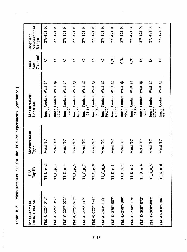
o oo @ @ o o _ o @ _ @ @ _ @ o= :_._ -= N -= .= -=- -= -= -= -= -=_ .= -= -=

_ N

c_ _. F- _- _-- F, {- [- [-- [-- F- [-- {-- _- _-,

_. ............

I

I I I I I I I I I I I I I

= f- [.- F. [- [- [-- _-. [-, [-, [.- (.I _- _-_)E

0 0 0 0 0 0 0 0 0 0 0 0

:_-- , ,

ii I I I I

.j_ _ = ,_ ' , , , , , , ,

[., [-, [-, [- [- _., _., [., [., [- {-, _..... _.i i iii ii __ i i i illlli i iii ii

B-17

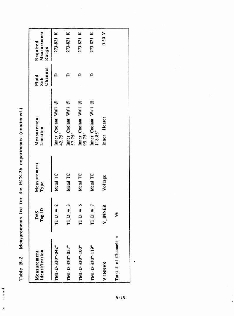
I I I

_e _ m m m• _ t_ p._

,._, = _t _ _

u,.,_ r,J

Appendix C

Measurement Uncertainty forthe ECS-2 Thermal Excursion Tests

Appendix C

Measurement Uncertainty forthe ECS-2 Thermal Excursion Tests

An extensiv_ measurement uncertainty analysis was conducted for themeasurements a_ad instrumentation used in the test fixture for the thermal

excursion experiments. Details of this analysis are documented in Wilkins

[Wilkins 1990]. Results of Wilkin's uncertainty analysis for tests conducted

in the ECS-2 test fixture are equally applicable for experiments conductedin the ECS-2b fixture since the instrumentation used in the two facilities is

essentially the same. A brief summary of the uncertainty analysis results

is given here to provide a measure of the uncertainty associated with the

data presented in this report.

Wilkins describes the potential error sources and the quantitative

contribution of each to the overall uncertainty in various key

measurements made during the ECS-2 test series. Those measurements in-clude:

(a) voltage and current to the test section (used to determine the inputpower to the test)

(b) air and water mass flows

(c) fluid and metal temperatures in the test section

(d) mass-energy balance

(e) absolute and differential pressures at selected points in the testsection

(d) contribution of the data acquisition system uncertainty to each ofthose measurements.

Possible error sources for the measurements were combined by theroot-sum-square (RSS) method of summing bias and precision errors, and

are given at the 95% (2_) confidence level. The single exception to this is

the metal thermocouple uncertainties, where bias errors were summed

algebraically in order to preserve the sign of the dominant bias term.

Equations appropriate for computing specific measurement uncertainties

(U) are given below. Table C-1 lists low- and high-range uncertainty

values for the measured parameters.

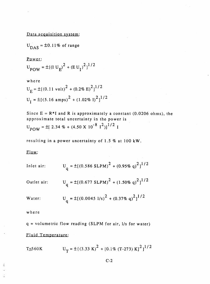
Data acquisition sysl;c_m;

UDA S = +_0.11% of range

Power:

2 )211/2Upo W=_+[(IUE) +(EU I

where

UE - _+[(0.11 volt) 2 + (0.2% E)2] 1/2

UI = +[(5.16 amps) 2 + (1.02% I)2] 1/2

Since E = R*I and R is approximately a constant (0.0206 ohms), the

approximate total uncertainty in the power is

Upo w = +[ 2.34 % + (4.50 X 10 -8 I2)] 1/2 I

resulting in a power uncertainty of 1.5 % at 100 kW.

F.EJ_o__w_:

Inlet air" U =+_[(0.586 SLPM) 2 +(0.95% q)2]l/2

q

Outlet air" U =_+[(0.677 SLPM) 2 + (1.50% q)2]l/2

q

_ )2 ]1/2Water: U =+[(0.0045 1/s + (0.37% q)2q

where

q = volumetric flow reading (SLPM for air, 1/s for water)

F!uid T e _.g.r_M.xl.L_

T<560K UT=_+{(3.33 K) 2 + [0.1% (T-273) K]2} 1/2

C-2I

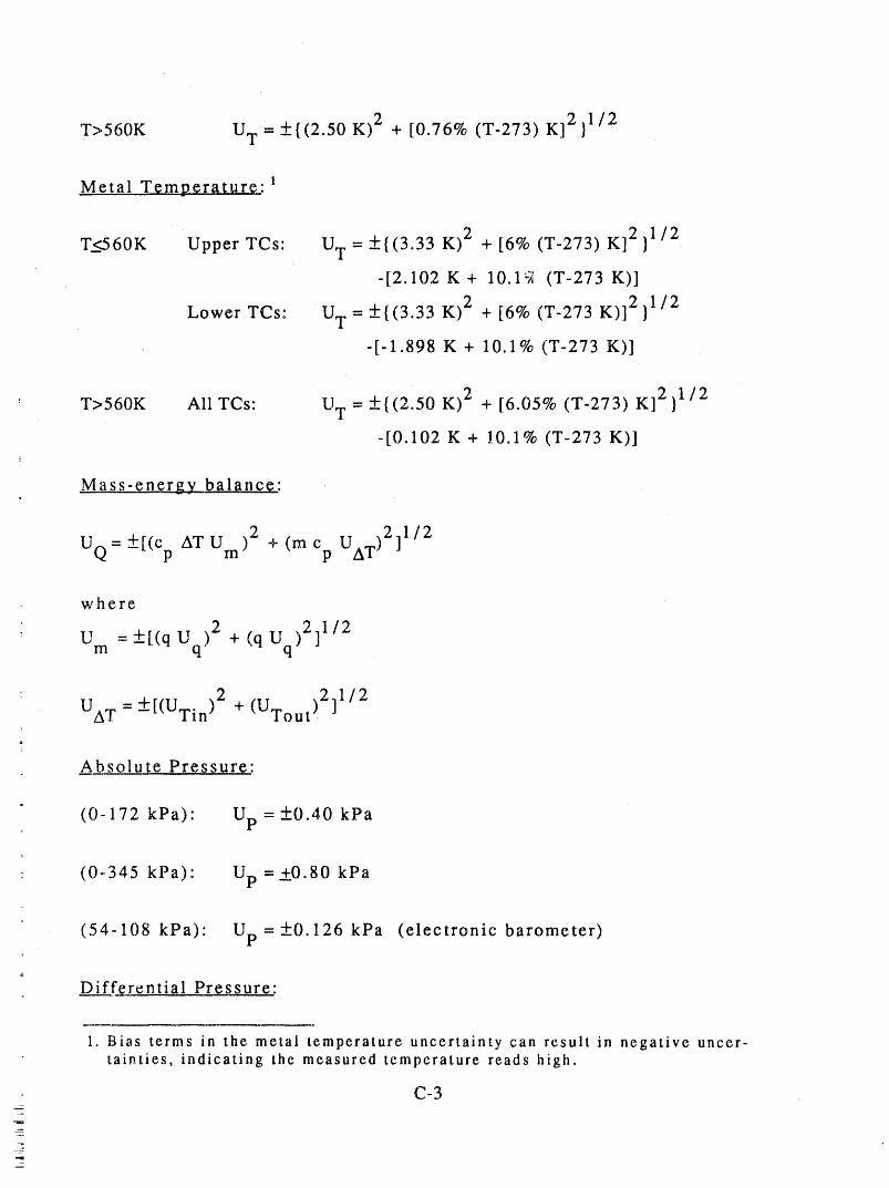
T>560K UT = -+{(2.50 K) 2 + [0.76% (T-273) K] 2 }1/2

Metal Temperatures- 1

T_<560K Upper TCs' UT = _{(3.33 K) 2 + [6% (T-273) K] 2 }1/2

-[2.102 K+ 10.1Y, (T-273 K)]

Lower TCs: UT = +{(3.33 K) 2 + [6% (T-273 K)] 2 }1/2

-[-1.898 K + 10.1% (T-273 K)]

" T>560K Ali TCs" UT=_+{(2.50 K) 2 + [6.05% (T-273)K]2} 1/2

-[0.102 K + ].0.1% (T-273 K)]

Mass-energy balance'

2 211/2UQ=_[(c ATU ) +(mc UAT)p m p

where

2 211/2U =_+[(qU ) +(qU )m q q

- UAT = -'+[(UTin )2 + (UTout)2]1/2m

_A.bsolu t_e Pressure:

(0- 172 kPa)" Up = +0.40 kPa

(0-345 kPa)' Up =+0.80 kPaz

(54-108 kPa)' Up=_+0.126 kPa (electronic barometer)

Differential Pressure'

1. Bias terms in the metal temperature uncertainty can result in negative uncer-tainties, indicating the measured temperature reads high.

C-3-2

-.

_

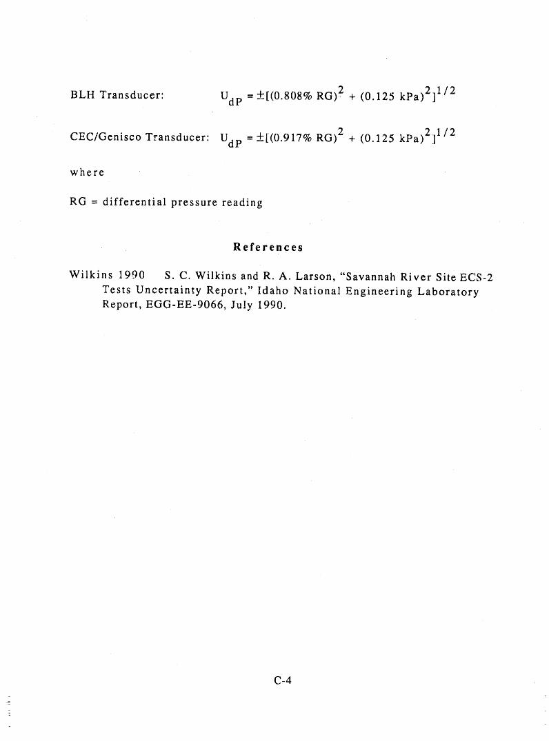
BLH Transducer: Udp =_+[(0.808% RG)2 + (0.125 kPa)2] 1/2

CEC/GeniscoTransducer: Udp =_+[(0.917% RG) 2 + (0.125 kPa)2]l/2

where

RG = differential pressure reading

References

Wilkins 1990 S.C. Wilkins and R. A. Larson, "Savannah River Site ECS-2

Tests Uncertainty Report," Idaho National Engineering LaboratoryReport, EGG-EE-9066., July 1990.

C'4

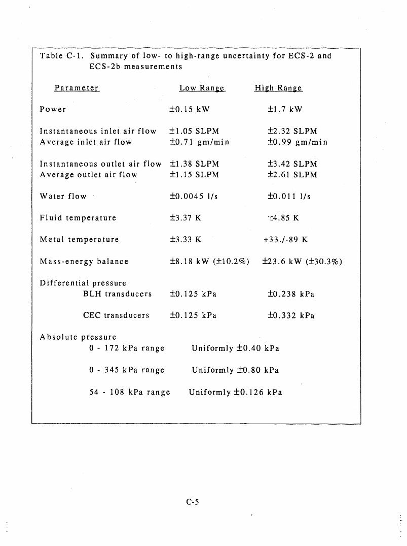
Table C-1. Summary of low- to high-range uncertainty for ECS-2 andECS-2b measurements

,Parame, ter Low Range, High Ran_.g&

Power _-+0.15 kW +1.7 kW

Instantaneous inlet air flow +1.05 SLPM +2.32 SLPM

Average inlet air flow +0.71 gm/min +0.99 gm/min

Instantaneous outlet air flow +1.38 SLPM +3.42 SLPM

Average outlet air flow _+1.15 SLPM _+2.61 SLPM

Water flow _+0.0045 1/s ±0.011 1/s

Fluid temperature -+3.37 K '_4.85 K

Metal temperature -+3.33 K +33./-89 K

Mass-energy balance +8.18 kW (_+10.2%) __+23.6 kW (_+30.3%)

Differential pressureBLH transducers _+0.125 kPa _-+0.238 kPa

CEC transducers _+0.125 kPa _+0.332 kPa

Absolute pressure

0- 172 kPa range Uniformly ___0.40 kPa

0- 345 kPa range Uniformly ___0.80 kPa

54 - 108 kPa range Uniformly -+0.126 kPa

C-5

Appendix D

Calculations Supporting Design/Performanceof the ECS-2 Inner Heater

Appendix D

Calculations Supporting Design/Performanceof the ECS-2 Inner Hev,_er

Numerical models were used to examine the performance

characteristics of the proposed inner heater design before the physicalheater was built. This appendix summarizes the mode!s constructed, dis-

cusses the performance of the inner heater relative to a production reactorfuel assembly, and presents conclusions of the conduction analysis con-ducted with these models. Additional analyses of the inner heater designare discussed in Appendix D of Reference [1].

Reference

[1] J.L. Anderson, K. G. Condie, and T. K. Larson, "Downflow Heat Transfer

in a Heated Ribbed Vertical Annulus with a Cosine Power Profile (Re-

suits from Test Series ECS-2b)," Idaho National Engineering LaboratoryReport, EGG-EAST-9144, July, 1990.

D-1

SUMMARY

A test apparatus is being designed at INEL that will simulate thermal

transient behavior of a Mark 22 assembly with fuel decay heat and low

coolant flow conditions. The apparatus design consists of two concentric

heated tubes which model the inner and outer Mark 22 fuel rings; downward

coolant flow will be introduced in the annulus between the tubes. The

purpose is to obtain thermal excursion data for the range of conditions

expected in the_Mark 22 assemblies during the ECS addition phase of a

hypothe_ical large-break Loss of Coolant Accident. Thermal

characterization studies were performed to:

(a) compare the transient response behavior of the test apparatus heated

tubes to the Mark 22 fuel rings,

(b) compare maximum temperatures of each test apparatus tube to its

corresponding Mark 22 fuel ring, assuming steady-state dryout of one

(90o) azimuthal sector and liquid film cooling of the remaining

sectors, and _

(c) determine adiabatic heatup rates for the test apparatus tubes.

The thermal response characteristics of the outer tube design were

determined to be nearly identical to those of the Mark 22 outer fuel ring.

The test apparatus response time constant was about 10% longer, and the

maximum temperature rise during sector dryout was 2% lower than for its

Mark 22 counterpart. The dimensions of the outer tube design and outer

fuel ring are nearly the same, and the outer tube electrical heater adds an

insignificant amount of thermal mass to the system.

For the inner tube design the response lime constant was about 2.4

times as long, and the maximum temperature rise about 14% higher than for

the Mark 22 inner fuel ring. The slower response was attributed to the

additional thermal mass required for inner tube heater design. The tube

thickness design value is considered a reasonable compromise between

thermal time constant and maximum temperature rise response

characteristics. Increased inner tube thickness would have increased the

system thermal mass, thus slowing the response time even further, while

decreased thickness would have increased the maximum temperature rise

D-2!

value. Thus, the selected tube thickness value represents the best match

of thermal response characteristics within the constraints of the heater

designrequirements. , i

The adiabaticheatupratesrepresentthe maximumratesobtainablewith

completeapparatusdryout. No credit is taken for azimuthalthermai

conduction;hence,the calculatedrates are significantlyhigher than

anythingexpectedduringthe thermalexcursionexperiments.The values

were 37,4 K/s for the innertubewith a heaterpower of 18.7 kW/ft

(44.6K/swith heaterpowerof 22.4 kW/ft),and 31.5 K/s for the outer tube

with a heater power value of 17 kW/ft.

D-3

CONTENTS

SUMMARY................................................................ D-2

i. INTRODUCTION..... , .................................... ............. D-6

2. SCOPEOF THERMALSTUDIES........................................... D-7

3. TWO-DIMENSIONALTHERMALCALCULATIONS............................... D-8

3.1 Computer Codes........... , ................. ................... D-8

3.1,1 ABAQUSFinite Element Code.......... ..................... D-83.1.2 PATRANComputer-Aided Engineering System ................. D-83.1.3 Calculational Sequence ................................... D-9

3.2 Test Apparatus Heated Tube and Mark 22 Fuel Ring Models ....... D-]O

3.2.1 Outer Tube Models... ..................................... D-]I3.2.2 Inner Tube Models ............................... . ........ D-123.2.3 Initial and Boundary Conditions .......................... D-I2

3.3 Results of Outer Tube Comparison ...................... ........ D-13

3.4 Results of Inner Tube Comparison .............................. D-15

4. TEST APPARATUSADIABATIC HEATUPRATES.............................. D-16

5. DISCUSSION AND CONCLUSIONS......................................... D-17

6. REFERENCES....................................... , ................ D-It

APPENDIX A-Listings of FORTRAN Programs that Transform PATRAN ModelBoundary Conditions into ABAQUS Input Cards............................ D-27

APPENDIX B-Supporting Calculations for SRL Test Apparatus and Mark22 Fuel Assembly Thermal Models........................................ D-31

APPENDIX C-PATRAN "Session" Files for Generating Inner and OuterTube Finite Difference Models.......................................... D-45

D-4

FIGURES

I. Cross section of a Mark-22 assembly.................................. D-19

2. Proposed configuration for the dual heated dryout heat transferexperiments......................................................... D-20

3. PATRAN / ABAOUS Calculation Flowchart................................ D-2]

4. Test apparatus and Mark 22 finite difference mesh models........... D-22

5. Test apparatus and Mark 22 outer tube thermal transient responses... D-23

6. Test apparatus and Mark 22 outer tube thermal time constants........ D-24

7. Test apparatus and Mark22 inner tube thermal transient responses... D-25

8. Test apparatus and Mark 22 inner tube thermal time constants......... D-26

__ D-5

z

L

I. INTRODUCTION

Heat transferexperimentsare to be performedat INELto supportthe safe

operationof the SavannahRiver Site productionreactors. One safetyconcern

is the thermalresponseof the Mark 22 fuel assembliesduringthe ECS addition

phase of a hypotheticallarge-breakLoss of CoolantAccident(LOCA). The_,

assembliesconsistof a seriesof concentrictargetand fuel ringsthat are

separatedby annularcoolantchannels,each dividedby ribs into four

azimuthalsectors,as shown in FigureI. The phenomenonof interestinvolves

the dryoutof one or more (90")sectors. Uncertaintiesexist in the

predictionof dryoutincipienceand the requirementsfor successfulrewet of a

dry surface,giventhe assemblyboundaryconditionsof inlet coolantflow and

fuel decay heat. Experimentalstudiesare desiredto obtainthermalexcursion

data for the rangeof conditionsexpectedin the Mark 22 assembliesduring the

ECS additionphaseof the hypotheticalLOCA.

J

A test apparatusis beingdesignedat INELthat will simulatethe thermal

transientbehaviorof the innerand outer fuel rings and the enclosedcoolant

annulus(designatedas Channel3 of FigureI).I lt will have the capability

to heat both the inner and outerwalls of the coolantannulus. Additionally,

it is to be constructedof reactor"typical"materials,i.e.,aluminum, lt

will use an existingdesignfor the innerheatedtube that simulatesa Mark 22

innerfuel; an outer heatedtube is being added to simulatethe outer fuel.

Figure2 showsthe proposedconfigurationof the test apparatus.

Calculationswere performedto characterizethe expectedthermalbehavior

of the test apparatusheatedtubes,and to comparethe transientresponse

characteristicsto those of Mark 22 assemblyfuel rings. The purposesof the

analyseswere: (a) to ensurethat the test apparatusinnerand outer fuel

rings will exhibitprototypica]transientthermalbehaviorduringthermal

excursiontests,and (b) to providemaximumheatuprate and temperature

informationto be used as guidancefor terminationcriteriafor the thermal

excursionexperiments.Detailsof the studiesare describedin the following

paragraphs.

I)-6

E

8

2. SCOPE OF THERMAL STUDIES

The thermal calculations included in the present document are outlined

below:

I. Transient thermal time constants were estimated for two-dimensional

(r-O) finite difference models of the test apparatus outer,heated tube

and the Mark 22 outer fuel ring. These models will be collectively

designated "outer tube models." The calculations were performed using the

ABAQUScomputer code. The results 2 indicated the _esirability for a

thinner-walled outer tube than was provided in the initial design.

Following the incorporation of this modification into the design, the

= calculation was repeated. Results of the final calculations are

presented. i

2. Similar calculations were also performed for r-O models of the test

apparatus inner tube and the Mark 22 inner fuel, collectively designated

as "inner tube models." This characterizationwas for information only,

because an existing inner heated tube design will be used for the

experiments.

3. Steady-state temperatures were calculated for the inner and outer tube

models, with heat source values representative of maximum test apparatus

power and coolant convection boundary conditions representing dryout of

- one (90°) sector.

4. Adiabatic heatup rates were estimated for the test apparatus heated tubes.

Items i, 2, and 3 were accomplished using the ABAQUS three-dimensional, finitei

element computer code, with a two-dimensional thermal mesh created using

PATRAN. Item 4 used simple hand calculations. The details of the thermal

calculations, the results, and the conclusions of the effort are contained in

the following sections.

_

u

I)-7

m

3. TWO-DIMENSIONALTHERMALCALCULATIONS

3.1 Computer Codes

3.1.1ABAQUS Finite Element Code °

The two-dimensional transient thermal response calculations were performed

using the ABAQUS3 computer code, using a finite element mesh generated using

PATRANPlus.4 ABAQUSis a general purpose, production oriented, finite

element code. lt is simple to use and has capabilities for a wide range of

nonlinear applications, one of which is the solution of three-dimensional,

transient heat conduction, or thermal diffusion, problems. Steady-state

solutions are obtained by direct integration of the spatial partial

differential equation. Transient solutions are obtained by integrating the

temporal/spatial equation with the backward difference operator (modified

Crank-Nichol son method).

3_1.2 PATRAN Computer-Aided Enqinee.rinqSystem

PATRAN Plus is an open-ended, general purpose, three-dimensional computer

aided engineering software system, lt includes the capabilities for

generating finite element meshes in cartesian, cylindrical, or spherical

coordinate systems, using automated command sequences. Element material

properties, volumetric heat generation rates for elements, and surface heat

flux values and convection heat transfer coefficients for edges can all be

specified. Translation of files from PATRAN to ABAQUS and back are done with

PATABA'and ABAPAT, respectively,which are supplied with the PATRAN Plus

software. The ABAQUS and PATRAN Plus software packages used for the

calculations comply with EG&G Quality Manual Section QP-21, Computer Software

Configuration Management.5 In addition, Hawkes performed verification and

benchmark calculations using these software packages.6 Results showed that

ABAQUS and PATRAN produced the correct solutions to heat transfer problems

when installed on INEL computers.

D-8

3.1.3 Calculational SeQuence_

The sequence of calculational steps is shown in Figure 3. PATRAN was used

to generate the model finite difference mesh, using input values for major

dimensional values (i.e. radii of inner and outer surface'sand rib corner

coordinates). The command sequence used to create the desired model is stored

in the ( ).ses file: the ( ).dat file contains the binary representation of

the current model plus a number of flags which control various display

options. The completed model was written to a "neutral," or interface, file,

the format of which is described in Chapter 29 of the PATRAN Plus User

Manual.3 The neutral file was input to a translator (PATABA) that converted

the model into the format required for ABAQUS. Present translator

capabilities are limited to conversion of node coordinates, making

node/element associations, and assigning material/property information to

element groups. This information forms the dimensional structure of the

ABAQUS input deck.

Model boundary conditions, material property tables, and transient control

information were entered manually into the ABAQUS [( ).inp] deck, as shown in

Figure 3. The boundary conditions (film heat transfer coefficients and heat

sources) are specified by: (a) input cards specifying the boundary location

and type, and (b) subroutines assigning the value. The input cards were

generated by the simple Fortran programs CONTRAN2, SHEAT, AND VHEAT. CONTRAN2

is used for surfaces with film heat transfer coefficient boundaryconditions,

and is maintained as a controlled document in the E&ST Software Index per E&ST

Group Standard Practice 4.0. SHEAT and VHEAT are versions of CONTRAN2

slightly modified to generate appropriate cards that specify distributed heat

sources for element surfaces or volumes. Listings for SHEAT and VHEAT are

contained in Appendix A; these two programs are not controlled versions, but

were shown to produce the correct boundary conditions via spot checks and

card-to-card consistency checks. The subroutines which assign values to the

boundaries are named FILM and DFLUX, and specify convection and heat source

values, respectively, as a function of azimuthal angle and transient time.

These values are applied to the model elements as specified by the input cards

described above. Material property tables and time step control parameters

were added to the ABAQUS input deck. The final step was to change the element

D-9

i

designations From the type supplied by PATRAN(S4R5) to diffusion-continuum,

2-dimensional, 4-node (DC2D4), which is recognized by ABAQUSas a heat

transf_er element. The ABAQUSfinite element code was then used to obtain the

transient thermal solutions.

As shown in Figure 3, three methods are available for obtaining plots.

The mesh representation can be plotted directly, as can any variable written

to ( ).fil. For the present application, the most useful directly-plotted

information was" the temperature response.

The method for obtaining color fringe plots required translating the

( ).fil information back to PATRAN-compatible form. Again, the translation

between the two major software items is not complete, and manual steps were

required to supplement the translation. The ABAQUSresults file is written

using internal data management routines in order to minimize computer I/0 cost

and disk storage requirements. The ABAQUS documentation offers sample coding,

the purpose of which is to convert the results file into ASCII format" i.e.,

to the ( ).fin file. The implementation of this coding is the CONVERT

program. The ABAPAT translator was then used to obtain a PATRAN-compatible

file containing the nodal temperature information required for the color

fringe plots.

The third plotting method used the Lotus I-2-3 PC software package, which

is capable of performing mathematical manipulations (e.g., logarithms and

least-squares linear fitting) of nodal temperature history data. The

translation was performed using TREAD, another implementation of ABAQUS sample

coding. The data were then downloaded to the PC and input to the I-2-3

spreadsheet program. The thermal time constants were obtained using this

procedure.

3.2 Test App_aratusHeated Tube and Mark 22 Fuel Rinq Models

Two-dimensional (r-#) transient thermal response calculations were

made to compare the thermal responses of the test apparatus outer heated tubes

and the Mark 22 assembly fuel rings. For each calculation, models of the test

apparatus tube and the corresponding Mark 22' fuel ring were included on the

D-10

_ o ;

±

same input deck so the results of the calculation could easily be compared.

Figure 4 shows the finite difference mesh models used for the calculation; the

top 90" section represents the test apparatus inner and outer tubes, and

the bottom 90" section represents the fuel rings of Mark 22 assembly.

Note there is no thermal connection between the two model sections.

3.2.1 OuterTube Models

The Test Apparatus outer tube is T6061 aluminum tubing with vertical

thermocouple grooves every 15" around the outer circumference. A heat

flux boundary condition is applied to the outer surface using etched foil

heaters, which consist of a thin (0.O05-in.) Inconel strip sandwiched between

two O.010-in.-thick mica sheets. An aluminum sheet, surrounding the tube,

forms a bridge across the thermocouple grooves to prevent local overheating of

the Inconel. The original design specified a 1.31S-inch tube inside radius, a

wall thickness of 0.125 in., and a 0.032-in. aluminum sheet. This design was

modified based on results of a preliminary thermal response calculation that

indicated the need for a thinner tube. The final dimensions, based on the

1.375-in. inside radius, were a wall thickness of 0.074 in. and an aluminum

sheet thickness of 0.016 in. The foil heaters were assumed to contribute a

negligible amount to the thermal mass of the outer tube, and were omitted from

the model. The Mark 22 outer fuel model was based on the dimensions in the

'Hydraulics Manual,7 and consists of the fuel tube portion frontthe log mean

radius inward.

The derivations of dimensional values for nodalization, heat flux boundary

conditions, etc., required to support the PATRAN and ABAQUS input values are

in Appendix B_ The PATRAN "session" files to create the inner tube models are

in Appendix C. Heat addition rate for the test apparatus outer tube was

240 kW/m2, based on maximum heater power of 22.4 kW. This was an early

design value; the present maximum heater power is 18.7 kW.I The Mark 22

model had a symmetry boundary at the log mean radius and included a uniformly

distributed heat source value of 225.2 MW/m3; this produces the same

steady-state heat flux at the inside surface as the 240 kW/m2 heat flux

value; thus, the two heat sources were equivalent.o

D-11

3.2.2 Inner Tube Models.... _

The test apparatus inner tube design is the same one to be used for the

ECS-2 thermal excursion experiment, lt has a heated 1'6061 aluminum tube with

a 2.211-in. outside diameter and a 0 O95-in. wall thickness. Four ribs are

affixed to the outer surface (at 90' intervals) and vertical thermocouple

grooves are machined into the inner circumference, spaced 15' apart. The

cross-section drawing, which shows the above details, is in the EOS.I

Details of the rib dimensions and arrangement are in drawing 430052. 8

Inside the tube is a MACORceramic insulator surrounding an Inconel tube

heater, which has an axially-varying wall thickness to simulate a non-uniform

axial flux profile. The Inconel heater dimensions are taken from drawing

4304379 and correspond to axial location 5, the location of maximum heat

flux. The corresponding Mark 22 inner fuel model was again based on the

dimensions in the Hydraulics Manual, and consists ef the portion from the log

mean radius outward.

As with the outer tube models, the derivation of the values used to

genel'ate the inner tube models is in Appendix B, and the PATRAN "session"

files that create the outer tube models are in Appendix C. The heat

generation rate for the test apparatus inner tube was 427.3 MW/m3, based on

a maximum linear heat generation rate of 17 kW/ft. The corresponding value

for the Mark 22 inner fuel ring was 207.8 MW/m3.

3.2.3 Initial and Boundary Conditions

The initial condition for the coolant channel surface of each model was a

heat transfer coefficient representative of forced convection to a liquid

falling film at I0 gpm flowrate (assumed typical of annulus low-flow ECS

conditions), and 311K. The calculation of this heat transfer coefficient is

in Appendix B of Reference 2; the value was 8800 W/m2-K. A steady-state

solution was obtained for this "wetted" condition. A transient condition was

then initiated by setting the convection heat transfer coefficient on half

(45") of each section to a low value (7.6 W/m2) to represent dryout of

one annular sector. The calculations were continued until a new steady-state

condition was achieved.

D-12

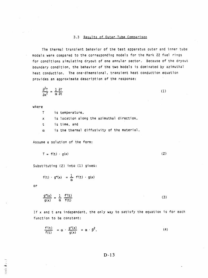
3.3 Results of Oul;erTube Comparison

The thermal transient behavior of the test apparatus outer and inner tube

models were compared to the corresponding models for the Mark 22 fuel rings

for conditions simulating dryout of one annular sector. Because of the dryout

boundary condition, the behavior of the two _odels is dominated by azimuthal

heat conduction. The one-dimensional, transient heat conduction equation

provides an approximate description of the response:

a2T i _T (i)ax2 a _t

where

T is temperature,

x is location along the azimuthal direction,

t is time, and

c_ is the thermal diffusivity of the material.

Assume a solution of the form:

T : f(t). g(x) (2)

Substituting (2) into (I) gives:

f(t). g'(x) = I_ f'(t)• g(x)

or

nx =g(___L)ig(x) a f(t)

i

If x and t are independent, the only way to satisfy the equation is for each

function to be constant:

g'(x) 132f'(t__.__)= a • -------= a. , (4)f(t) g(x)

D-13

-_

where the form of Eqn. (3) suggests that the constant is some multiple of _.

For any fixed location on the models, the thermal response is approximately

described by:

f = CI e_zt.

Using the initial and final conditions of the problem gives:

Tf - T(t) = e_t/_ (5)Tf - Ti

where

T(t) is the transient thermal response,

Ti is the initial temperature,

Tf is the final temperature, and

x is the thermal time constant.

The linear form of this equation is

In [Tf- T(t)]= t/_ + In [Tf- Ti] (6)

Figures 5 and 6 show the thermal responses of the outer tube models for the

location at the center of the dryout patch (the symmetry boundary at the 0°

azimuthal position). Figure 5 is temperature versus time, and Figure 6 shows

In (Tf - T) versus time and the corresponding least-squares fitted lines for

calculated temperatures at the center of the dryout patch (0°).

The regression results were, at the center of the dryout region:

Test Apparatus : In (722.51 - T) - _t / 7.69 + In (416.98)

Mark 22: In (731.07 - T) = -t / 7.02 + In (414.45)

Hence, the thermal time constants were:

Test Apparatus 7.7 s

Mark 22 7.0 s

D-14

The resul_,sof the calculation for steady-state maximum temperature with

dryout conditions were'

Test Apparatus 722 K

Mark 22 731 K

The steady-state temperatures of the test apparatus with the dryout

boundary condition were nearly identical to those calculated for the Mark 22

outer fuel ring; the temperature rise of the test apparatus model was g8% of

that calculated for the Mark 22 model. Thethermal time constants also agreed

closely; the test apparatus response was slower because of the larger thermal

mass and lower thermal conductivity of the T6061 test apparatus tube compared

to U-AI (fuel) and aluminum (cladding) used in the Mark 22 model.

3.4 Results of Inner Tube _omparisQ_

Figures 7 and 8 show the thermal responses of the inner tube models for

the location at the center of the dryout patch (the symmetry boundary at the

O' azimuthal position). Figure 7 shows temperature versus time, and

Figure 8 shews In (Tf - T) versus time. The corresponding linear

least-squar,_sfitted equations are"

Test Apparatus : In (517.74 - T) - -t / 10.04 + In (141.25)

Mark 22" In (497.22 - T) - -t / 4.14 + In (155.19)

Hence, the thermal time constants were"

Test Apparatus 10.0 s

Mark 22 4.1 s

The results of the calculation for steady-state maximum temperature with

dryout conditions were"

Test Apparatus 594 K

Mark 22 566 K

D-15

The steady-statetemperaturesof the test apparatuswith the dryout

boundaryconditionare slightlyhigherthan for the Mark 22 inner fuel ring.

(Totaltransienttemperaturerise is about 14% higherfor the test

apparatus.) However,the thermalresponseof the test apparatusis

significantlyslower. The differencein temperaturerise is due to the

differencein thermalconductivityof T6061 aluminumand that of the Mark 22

fuel and cladmaterials. The slowerresponseis becauseof the mass of the

Inconelheaterand the MACOR insulatingtube; wall_thicknessesof the test

apparatustube itselfand the Mark 22 fuel ring are comparable.

4, TESTAPPARATUSADIABATICHEATUPRATES

Adiabaticheatuprateswere determinedfor the inner and outer tubes of

the test apparatus. These are the heatuprates for the theoreticalcase of

completedryoutof the apparatus. The calculationprovidesan estimateof the

maximumheatuprates attainable,for use in designof test apparatus

protectionsystems. Detailsof the calculationsare in AppendixB. Outer

tube calculationswere done for maximumheaterpowervaluesof 22.4 kW and

18.7 kW. The resultswere heatuprates of 44.6 and 37.4 K/s, respectively.

For the innertube, a maximumheaterpower valueof 17 kW/ftwas used; the

cal'culatedheatuprate was 31.5 K/s.

D-16

5. DISCUSSIONANDCONCLUSIONS

The calculated thermal response characteristics of the test apparatusouter tube were nearly identical to those of the Mark 22 outer fuel tube

model. Transient temperature rise was 2% lower than for the Mark 22 model and

the estimated thermal time constant was about 10% slower. Based on the

similarity of response of the thermal models, the test apparatus outer tube

_hould_e nearlyindistinguishablefroma Mark 22 outer fuel ring for equal

setsof boundaryconditions. Calculationsfor the innertube thermalmodels

also showedresponsesvery similarto the Mark 22 inn.erfuel ring. The

differencesare due to the lowervalue of test apparatusazimuthalconduction

and the heater,which adds a significantamountof thermalmass to the

system. The originalthermalstudies,performedby Schroeder,I0 were done

to provideresponsesimilarityfor transienttimes of up to about30 seconds.

The tube thicknessfinal designvaluewas a reasonablecompromisebetween

overalltransientresponsetemperatureriseand the thermaltimeconstant. A

thickertubewould increasethe thermalmass, thus slowingthe responsetimeeven further. A thinnertubewould have furtherreducedthe azimuthal

conductionof the system. Thus, the selectedvalue for tube thickness

representedthe bestcompromisebetweenheaterdesign requirementsand

fidelityto prototypicalthermalbehavior. These results,i.e.the0

demonstrationof closelymatchedthermalcharacteristicsfor both test

apparatustubes, indicatesthat the thermalbehaviorof the entireapparatus,

includingthe enclosedcoolantannulus,shouldprovidethe best prototypical

behaviorattainablefor the given designconstraints.

The adiabaticheatuprates representthe maximumrates attainablefor the

given heat inputvalues. The calculatedratesare significantlyhigherthan

the resultsof the transientcalculations(Figures5 and l), which indicate

averageheatuprate valuesof -25K/s. The azimuthalconduction

characteristicsof the system,and the assumptionof one (90")dry sector,

significantlyreducesthe rate to far belowthe adiabaticrate.

D-17

6. REFERENCES

I. J.L, Anderson,T.K. Larson,H.N. Romero,Experimental.OI)eratinqS_12ecjfic.ations,.DualHeatedECS H..eatTransferExper_ilmen_s(draft),July 5,1989.

2, J.E. FisherItr to J.R. Wolf, "Resultsof ThermalResponseCalculationsfor SRL Dual HeatedECS HeatTransferExperimentOuter Tube," EG&GInterofficeCorrespondenceJEF-03-89,August7, 1989.

3. ABAQUSU_sersManual,Version4.7, Hibbitt,Karlsson& Sorensen,Inc.,1988.

i

4. .PATR.ANPlus User Manual.Volumesi and II, Release2.3, PDA Engineering,CostaMesa, California,July 1988.

.. 5. _E.G&GIdaho,lhc Qualit.yManual,Issue 14, March 17, 1989, DocumentNo. QP-21.

6. G.L.Hawkes,Verificationand Bench.markinqof ABAOUSand_PATRANfor HeatTransferApolications,EGG-EAST-8680,to be published.

7. _Hvdr_aulicsand Hea..tTransferof Mark 22 Fuel Assembli_es,DPSTM-22(H),RevisedNovember1974.

8. SavannahRiver Site INEL-ECS..2 DryoutExperimentAluminumHeaterTube,EG&G IdahoDwg. 430052,June 1989.

9. S.ava..nnahRiver Site INEL-ECS.2 DryoutExperimentHeaterTube Assembl.z,EG&G Idaho Dwg. 430437,July 1989.

10. J.A. Schroeder,privatecommunication,9-21-1989.J

D-18

/

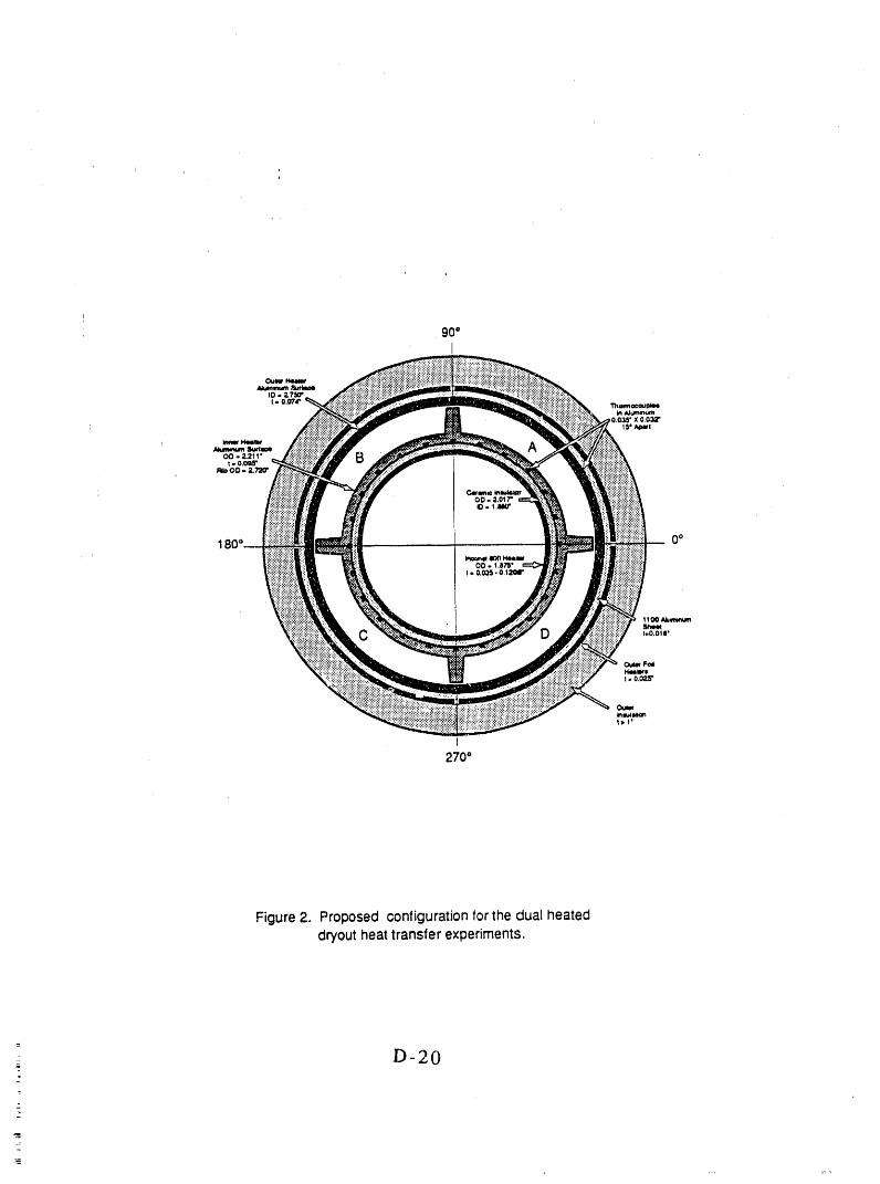
Figure 2. Proposed configuration for the dual heated

dryout heat transfer experiments.

=

D-20=

_

_

l ii_= comman'ds J

1F)'°" '!"t* .I.

Y i

I NEUTRAL [( ).out] FI_

JJt qf

l,, (Boundary Condl't'ion .....'j FPATABA-(Transla'i'or)J

, C_N_ _ [I'vHEATI us'er Subroutines---T-'-" Material Properties

[ABAQUS [( ).inp] FILE j

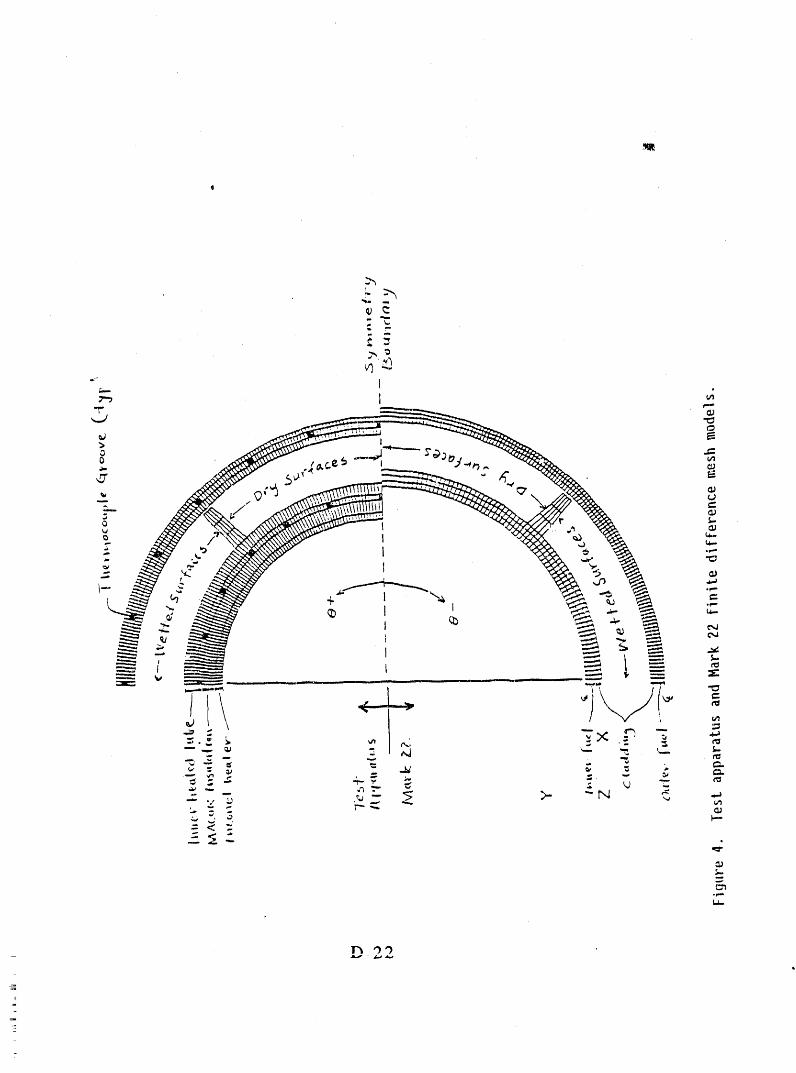
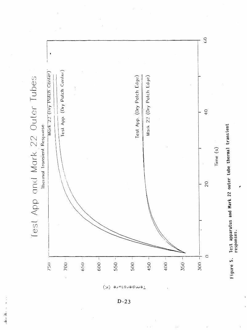
jco.v_.,_(,oAse,,![i li 'l i

I"'ABAPAT iTrans/ator)J_ [ Lotus 1-2-'_ J

Figure 3. PATRAN / ABAQUS Calculation Flowchart

D-21

0

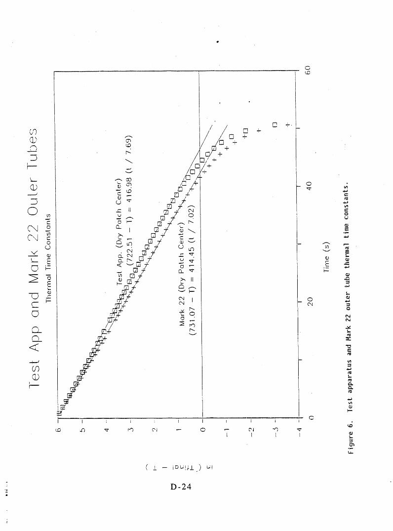
0t.D

(± --iou!_-±) ul

= D-24

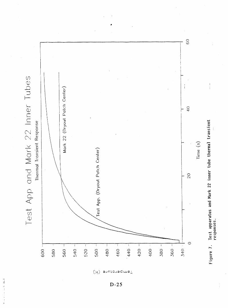
0uD

D-25

__

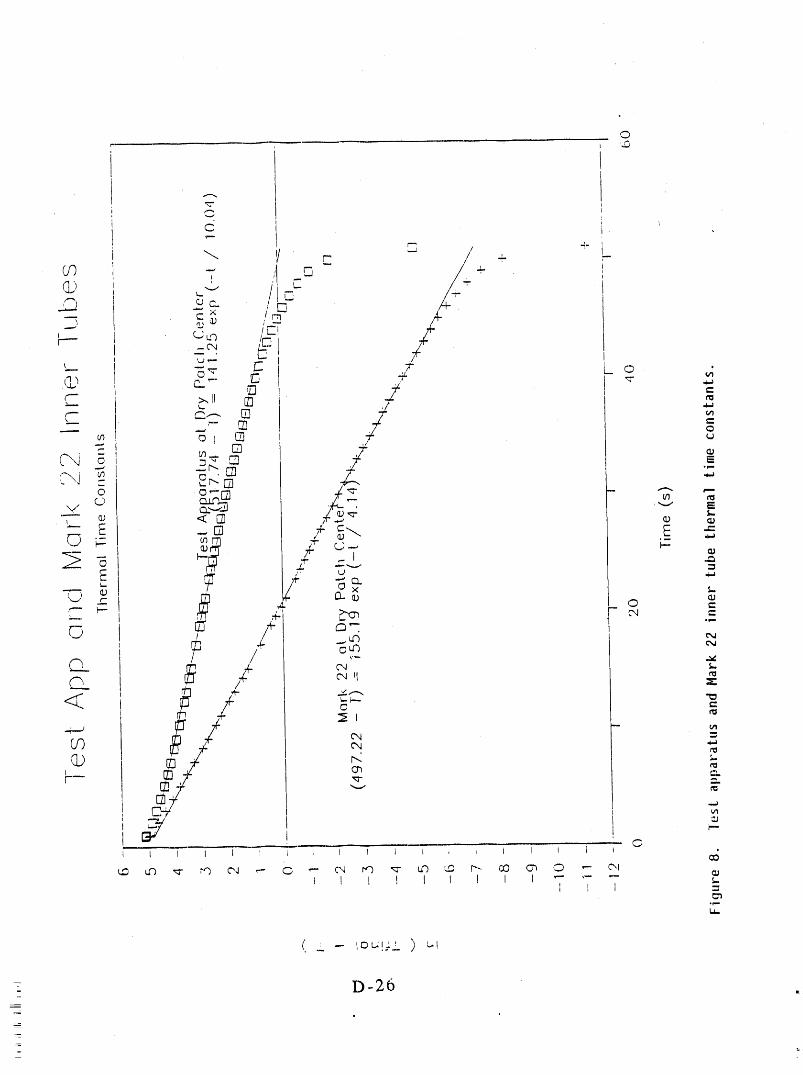
0

( _ -lc,u!;-& ) ul

2 D-26--

___

_=

APPENDIXA

Listingsof FORTRANProgramsthat Transform

PATRANModelBoundaryConditionsintoABAQUS InputCards

D-27

J

=

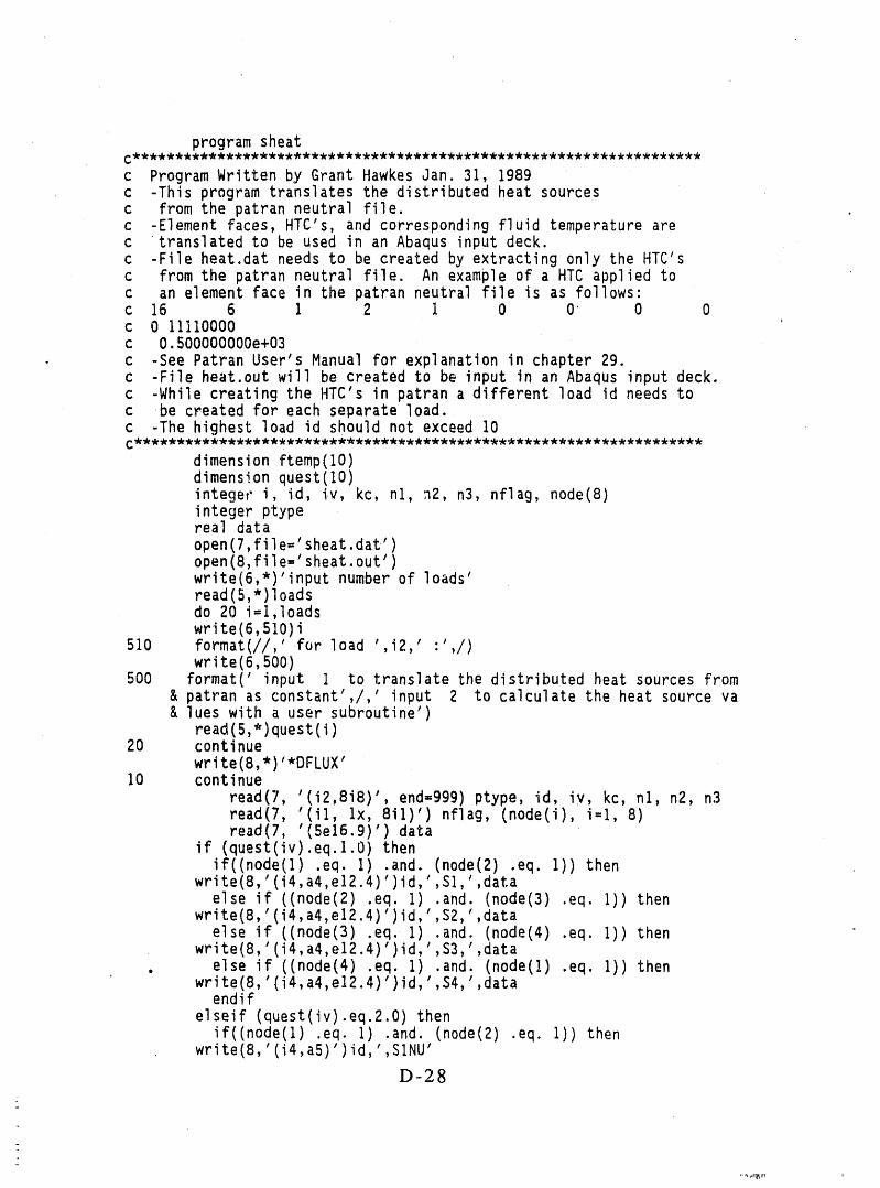
program sheat

c Program Written by Grant Hawkes Jan. 31, 1989c -This program translates the distributed heat sourcesc from the patran neutral file.c -Element faces, HTC's, and corresponding fluid temperature arec translated to be used in an Abaqus input deck.c -File heat.dat needs to be created by extracting only the HTC'sc from the patran neutral file. An example of a HTC applied toc an element face in the patran neutral file is as follows:c 16 6 I 2 I 0 O 0 0c 0 11110000c O.500000000e+03

. c -See Patran User's Manual for explanation in chapter 29.c -File heat.out will be created to be input in an Abaqus input deck.c -While creating the HTC's in patran a different load id needs toc be cmeated for each separate load.c -The highest load id should not exceed 10

dimension ftemp(lO)dimension quest(lO)integer i, id, iv, kc, nl, _2, n3, nflag, node(8)integer ptypereal data

open(7,file='sheat.dat')open(8,file:'sheat.out')write(6,*)'input number of loads'read(5,*)loadsdo 20 i:1,1oadswrite(6,510)i

510 format(//,' for load ',i2,' :',/)write(6,500)

500 format(' input I to translate the distributed heat sources from& patran as constant',/,' input 2 to calculate the heat source va& lues with a user subroutine')

read(5,*)quest(i)20 continue

write(8,*)'*DFLUX'10 continue

read(7, '(i2,8i8)', end-999) ptype, ld, iv, kc, nl, n2, n3read(7, '(ii, Ix, 8ii)') nflag, (node(i), i=l, 8)read(7, '(5e16.9)') data

if (quest(iv).eq.1.0)thenif((node(1) .eq. I) .and. (node(2) .eq. I)) then

write(8,'(i4,a4,e12.4)')id,',SI,',dataelse if ((node(2) .eq. i) .and. (node(3) .eq. I)) then

write(8,'(i4,a4,e12.4)')id,',S2,',dataelse if ((node(3) .eq. I) .and. (node(4) .eq. I)) then

write(8,'(i4,a4,e12.4)')id,',$3,',data. else if ((node(4) .eq. I) .and. (node(1) .eq. I)) then

write(8, '(i4,a4,e12.4)')id,',S4,',dataendif

elseif (quest(iv).eq.2.0) thenif((node(1) .eq. I) .and° (node(2) .eq. I)) then

write(8,' (i4,a5)')id, ',SINU'

D-28

else if ((node(2).eq.I) .and.(node(3).eq.I)) thenwrite(8,'(i4,aS)')id,',S2NU'else if ((node(3).eq.I) .and.(node(4).eq.I)) then

write(8,'(i4,a5)')id,',S3NU'else if ((node(4).eq.I) .and.(node(1).eq.I)) then

write(8,'(i4,a5)')id,',S4NU'endif

endifgo to 10

999 continueclose(7)close(8)stopend

D-29

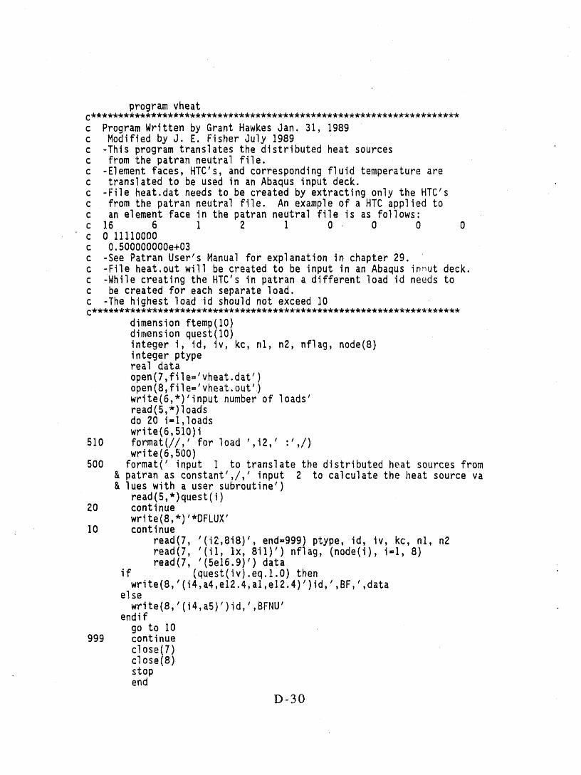
programvheatC _**_*****_*_**_,_***__****_*_**_**_._***_**_,_ _*

c ProgramWrittenby Grant HawkesJan. 31, 1989c Modifiedby J. E. FisherJuly 1989c -Thisprogramtranslatesthe distributedheat sourcesc from the patranneutralfile.c -Elementfaces,HTC's,and correspondingfluidtemperaturearec translatedto be used in an Abaqus inputdeck.c -Fileheat.datneedsto be createdby extractingonly the HTC'sc fromthe patranneutralfile. An exampleof a HTC appliedtoc an elementface in the patranneutralfile is as follows:c 16 6 I 2 I 0 0 0 0

' c 0 11110000c O.500000000e+03c -See PatranUser'sManualfor explanationin chapter29.c -Fileheat.outwill be createdto be input in an Abaqus in_utdeck.c -Whilecreatingthe HTC's in patran a differentload id needs toc be createdfor each separateload.c -Thehighestloadid shouldnot exceed 10

dimensionftemp(10)dimensionquest(t0)integeri, ld, iv, kc, nl, n2, nflag,node(8)integerptypereal dataopen(7,file='vheat,dat')open(8,fiIe='vheat,out')write(6,*)'inputnumberof loads'read(5,*)loadsdo 20 i=1,1oadswrite(6,510)i

' for load ' i2 ' ' /)510 format(//, , , : ,write(6,500)

500 format('input I to translatethe distributedheat sourcesfrom& patranas constant',/,'input 2 to calculatethe heat sourceva& lueswith a user subroutine')

read(5,*)quest(i)20 continue

write(8,*)'*DFLUX'10 continue

' 8i8)' end=g99)ptype,id, iv, kc, hl, n2read(7, (i2, ,read(7,'(ii,lx, 8ii)')nflag, (node(i),i_I, 8)read(7,'(5e16.9)')data

if (quest(iv).eq.1.0)then' a4 e12 4 al e12.4)' ' BF ' datawrite(B, (i4, , . , , )ld, , , ,

else' aS)' ' BFNU'write(8, (i4, )id, ,

endifgo to 10

999 continueclose(7)close(8)stopend

D-30

APPENDIXB

SupportingCalculationsfor SRE.Test Apparatus

and Mark 22 FuelAssemblyThermalModels

D-31

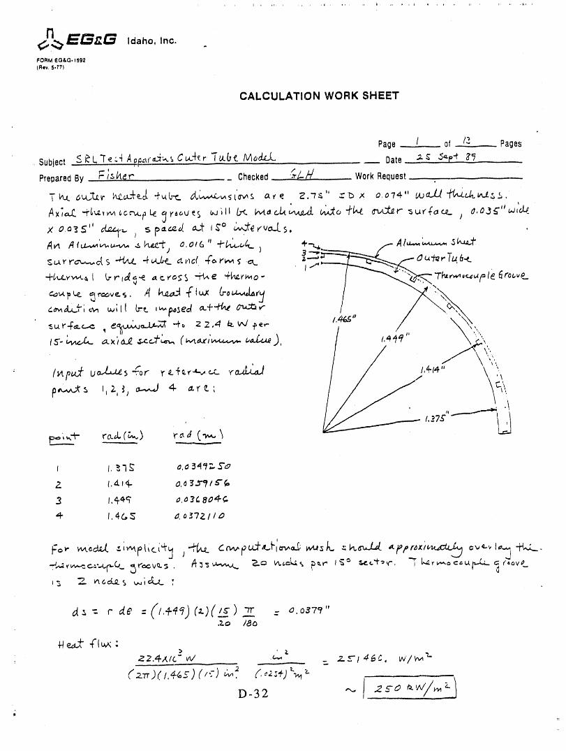
_E_G Idaho,Inc. .FORM eO&O.lSg2

(Rev. 5./'71

CALCULATION WORK SHEET

4" /,4GS 4o_7ZI1_

d, 0,g79 "

._o /8o

44e,# -¢I_ :z 2,4A./c" vv' ,_., ,. "u= 2.._/4._. w'/_

(__r_)(_.4_-) (_,:) " _ ,.._. _. (,.'_s+Ja

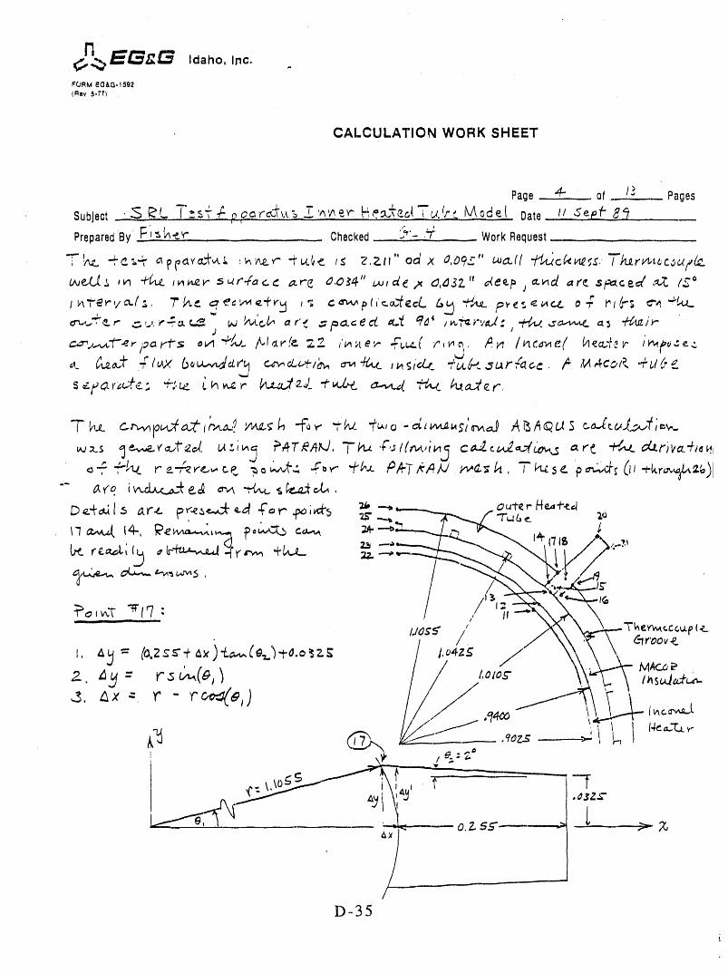
FORM EG&O*1592

(Rev 5-77)

CALCULATION WORK SHEET

Page 4- of /3 Pages

Subject ._ _' L. _._ _ _ -1:-"; o m :_ u. % E 'A '_ _ _ ,Ic-__ _ tc,( _ ,M.(:_ .k,_.Gd _ ( [Date t/ 5e p _8_

PreparedBy FI ._I_.C¥" ...... Checked _,_"-,_ WorkRequest

"_.t/_C. "f, _ ;_ _ p_O,'_'_.l, ,,_'_ _" "_ _.(I< tS' "Z,2.II" od X 0,09Z" _ucC(f "{4.,_¢kv_.;, "T'J_r_t,.c_f(.E_

u_e.(.1.; ,v_ _ _v" 5_r#a<.¢ _r_ o.ot4" L_, de ,x 6,d3Z " _ecp ; _d =rc =i_¢ea[ ,._Z. /,C°

I',_"r_._v_(; "7"_¢ _,ec'_¢+r_ ,; cu_,,p(,_¢cL (..,_ _.,v_ p_,e,.,_-,t.z, e.:. rl(r'; c.'..,."":.eL

J

n

FORM EG&G-1592

(Re¥. 5-771

CALCULATION WORK SHEET

Page "_" of /_ Pages

Subject SI_'L. Tes_ _ p/_=vo_.'_L.tS_v_-v" _ecc.+_'T, _.x{a't t_L._.._ Bate.. (I _,:.(_.r _

PreparedBy ( i- l_1- Checked "-_/ _ WorkRequest

. ._, / ,y\)\ I, t o ,._"

D-36

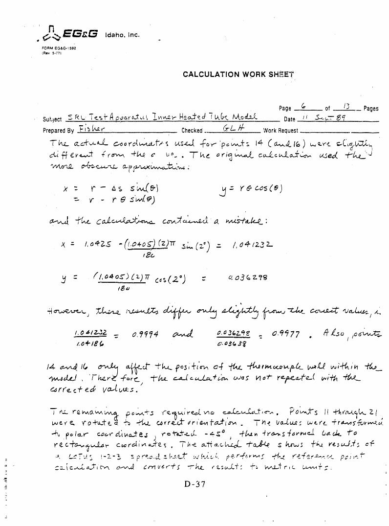
FORM EG&G-1592(Rev 5-77)

CALCULATION WORK SH,_E'_:

Page (" of /-_ Pages

Sub)ect < r<L "[_s_'_.p?_Y'_._'_. "l'wv_'r _.o._erJ "[Lk(J't /vLocLt_ /I 5--- _"' _ '- Date C:-

PreparedBy ."__'_(/_-_' Checked _/-.-- }'/" WorkRequest

, # i !

• i

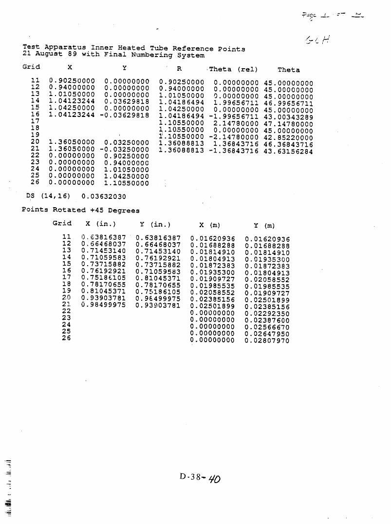
'_ _ j t'¸

Test Apparatus Inner Heated Tube Reference Points21 August 89 with Final Numbering System

Grid X Y K Theta (re I) Theta

11 0.90250000 0.00000000 0.90250000 0.00000000 45o0000000012 0.94000000 0.00000000 0.94000000 0.00000000 45.0000000013 1.01050000 0.00000000 1.01050000 0.00000000 45.0000000014 1.04123244 0.03629818 1.04186494 1.99656711 46.9965671115 1.04250000 0o00000000 1.04250000 0.00000000 45.0000000016 1.04123244 -0.03629818 1.04186494 -1.99656711 43.0034328917 1.10550000 2. 14780000 47.14780000

18 ' 1.10550000 0.00000000 45.0000000019 I'.10550000 -2.14780000 42.8522000020 1.36050000 0.03250000 1.36088813 1.36843716 46.3684371621 1.36050000 -0.03250000 1.36088813 -1.36843716 43.6315628422 0. 00000000 0. 9025000023 0. 00000000 0. 9400000024 0. 00000000 1. 0105000025 0. 00000000 1. 0425000026 0. 00000000 I. 10550000

DS (14, 16) 0.03632030

Points Rotated +45 Degrees

Grid X (in.) Y (in.) X (m) Y (m)

11 i'),,63816387 0. 63816387 0 .01620936 0 .0162093612 0 66468037 0.66468037 0.01688288 0.0168828813 0.714-=3140 0.71453140 0.01814910 0.0181491014 0.71059583 0.76192921 0.01804913 0.0193530015 0 •73715882 0 •73715882 0 •01872383 0 •0187238316 0.76192921 0.71059583 0.01935300 0.0180491317 0 .75186105 0 •81045371 0 •01909727 0 •0205855218 0 •78170655 0. 78170655 0 .01985535 0 •0198553519 0 •81045371 0 .75186105 0 .02058552 0 •0190972720 0. 93903781 0 •9_499975 0 .02385156 0 .0250189921 0. 98499975 0. 93903781 0 •02501899 0. 0238515622 0 •00000000 0 •0229235023 0 •00000000 0 •0238760024 0.00000000 0 0256667025 0 •00000000 O. 0264795026 0 .00000000 0 •02807970

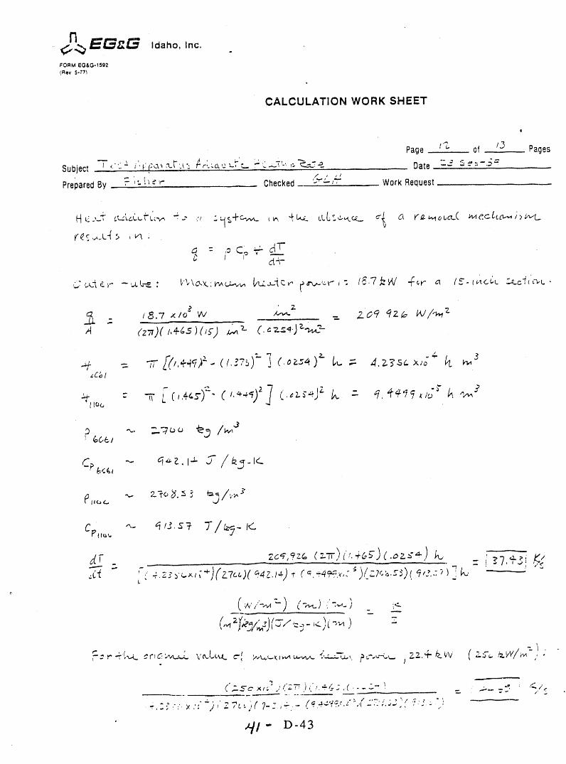
n_ E_'_' Idaho, Inc. .FORM EG&G-1592

(Rev 5-771

CALCULATION WORK SHEET

I

Page t% of /.3 Pages

Subject "T,. -' ;'r:(:,.-t_m_':t- _,-:.:cL,-L,"_ _C..-.'-',;_-_.._':_ Date "'= <"-':-

PreParedBy ? ,,. !_ s r-. Checked ""-:,-- Work Request

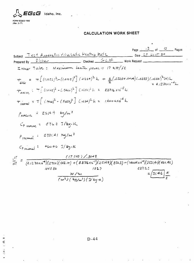
r_ ._'_' Idaho, Inc.

FORM EG&G-1592

(Rev. 5-77)

CALCULATION WORK SHEET

t

Page i_ of /3 Pages

Subject -I _-'_ _t;R _v_'_S r!.-(_.(ju..:_i<. _cc.Jr'c,.p _.{% Date ":" _c,;..T" 3=

PreparedBy _- i& !,_-_- Checked S-r-/--_ Work Request "

v_._.r "T_Ltr_ " /Vt_×/_._ _- _-¢_-._._ pr_.t. ,_ /7 _W/F{

6cGl 2. / _..,D/_ I C

" iV ,IA/'(3P_ *

. /-(,._ J -.,_t.c_,-_: "T ._,) . (.,_zs)_- C._.._)L _ - /.4oo_.x_o L

z

"_ D-44

,/

I,/

,I,

APPENDIXC

PATRAN "Session"Files for Generating

Innerand OuterTube FiniteDifferenceModels

D-45

-

Outer Tube Models

1._-_!.0 - 7 o

Inner Tube Models

- D-4 9/.,_U=j

Appendix E

Calculated Parameters for the ECS-2

and ECS-2c Thermal Excursion Experiments

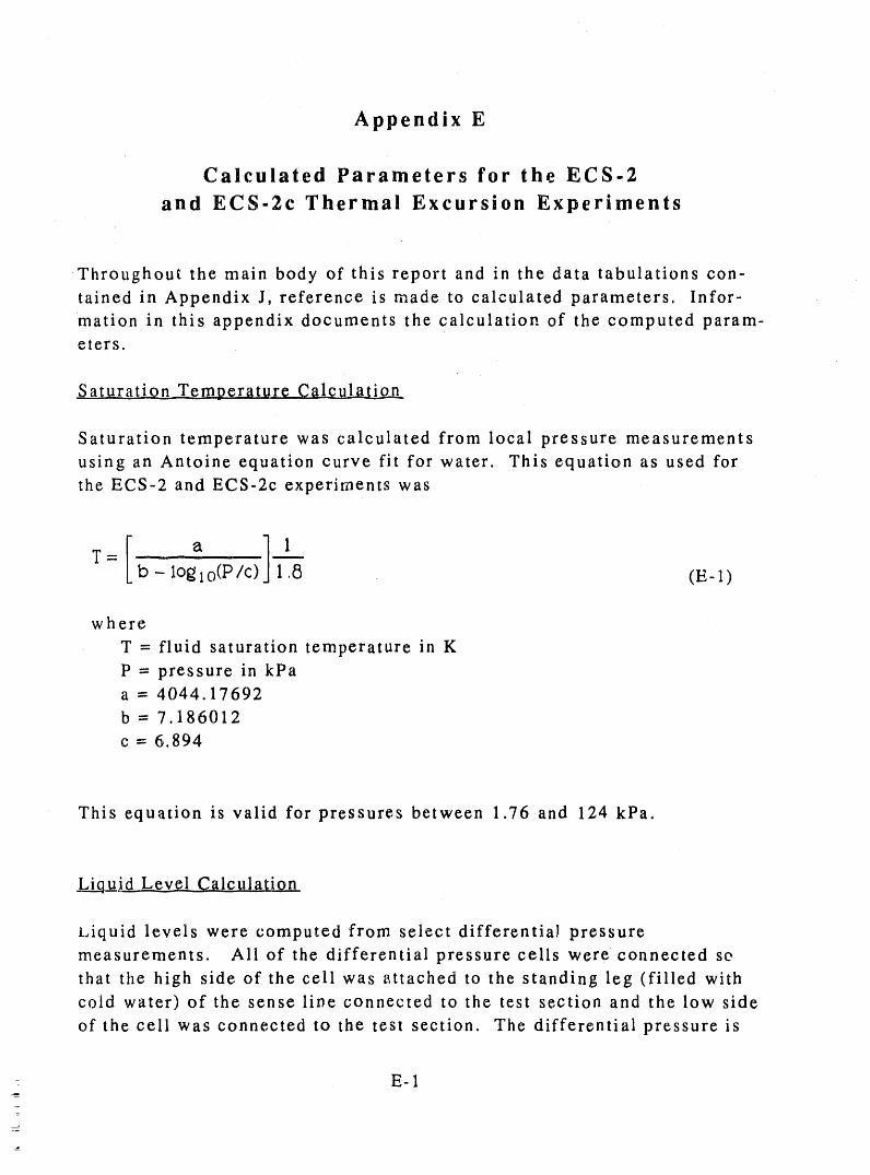
Appendix E

Calculated Parameters for the ECS-2

and ECS-2c Thermal Excursion Experiments

Throughout the main body of this report and in the data tabulations con-

tained in Appendix J, reference is made to calculated parameters. Infor-

mation in this appendix documents the calculation of the computed param-eters.

Sat uratio_ Temperature Ca!c_

Saturation temperature was calculated from local pressure measurements

using an Antoine equation curve fit for water. This equation as used for

the ECS-2 and ECS-2c experiments was

_ _a ] 1T = b -S lo_- 1o(1:>/C) 1.8 (E-l)

where

T = fluid saturation temperature in K

P = pressure in kPaa = 4044. 17692

b = 7.186012

c = 6.894

This equation is valid for pressures between 1.76 and 124 kPa.

.Li_L_i_ddLevel _Calculation

Liquid levels were computed from select differentia{ pressure

measurements. All of the differential pressure cells were connected se

that the high side of the cell was attached to the standing leg (filled withcold water) of the sense lioe connected to the test section and the low side

of the cell was connected to the test section. The differential pressure is

E-1

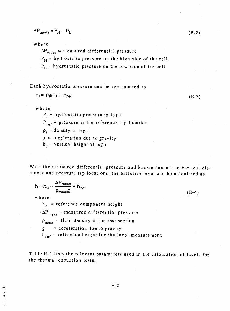
APmoas = PH - PL (E-2)

where

APrn_a_ = measured differential pressure

PH = hydrostatic pressure on the high side of the cell

PL = hydrostatic pressure on the low side of the cell

Each hydrostatic pressure can be represented as

Pt = Pi_h_ + Prcf (E-3)

where

Pi = hydrostatic pressure in leg i

Prcf = pressure at the reference tap location

Pi = density in leg i

g =- acceleration due to gravity

h i = vertical height of leg i

With the measured differential pressure and known sense line vertical dis-tances and pressure tap locations, the effective level can be calculated as

h h c APmeas '= - -..__--.__ + hre IPmoas_ (E-4)

where

h e = reference component height

APrne,,s = measured differential pressure

Pmeas =" fluid density in the test section

g = acceleration due to gravity

hre f --- reference height for the level measurement

Tablc E-1 lists the relevant parameters used in the calculation of levels forthe thermal excursion tests.

1,-2

=2=

?

=

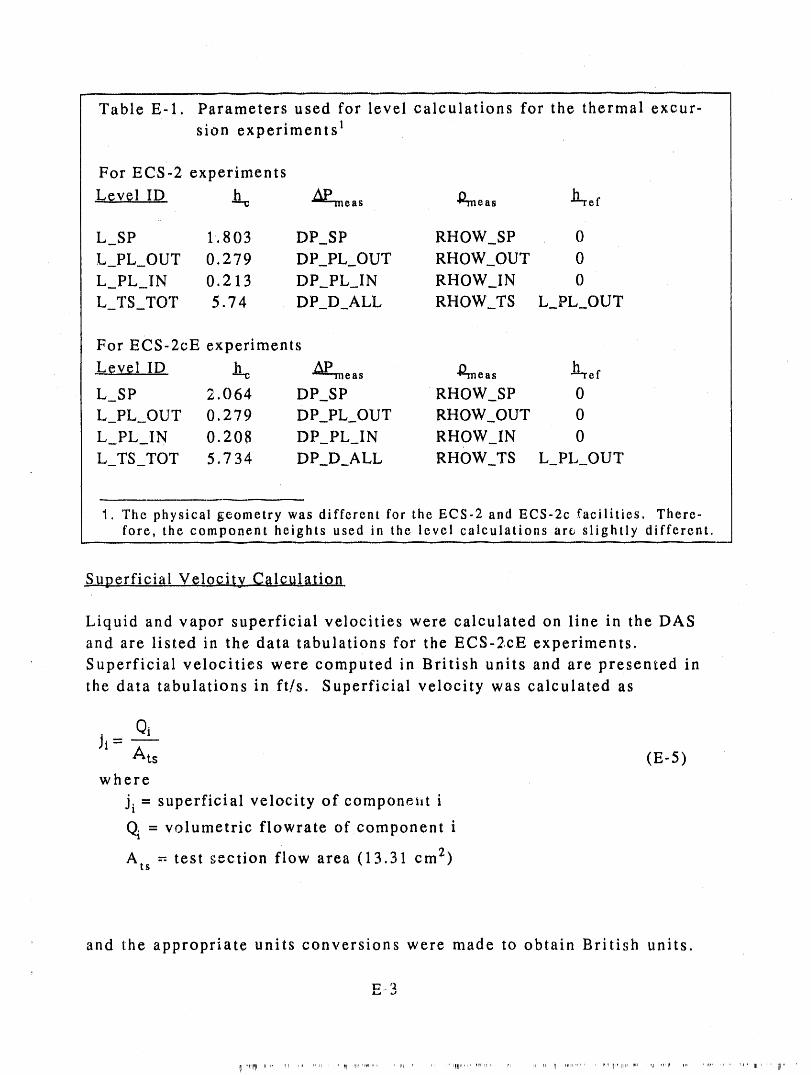
Table E-1. Parameters used for level calculations for the thermal excur-

sion experiments 1

For ECS 2 experiments

Level ID -_ _--'me as '12meas "l]"re f

L_SP 1 803 DP_SP RHOW SP 0

L_PL_OUT 0.279 DP_PL_OUT RHOW OUT 0

L_PL_IN 0.213 DP_PL_IN RHOW_IN 0

L_TS_TOT 5.74 DP_D_ALL RHOW_TS L_PL_OUT

For ECS-2cE experiments

_Level ID h_..e _-_-'meas "0"m_as "b'-ref

L_SP 2.064 DP_SP RHOW_SP 0

L_PL_OUT 0.279 DP_PL_OUT RHOW_OUT 0

L_PL_IN 0.208 DP_PL_IN RHOW_IN 0

L_TS_TOT 5.734 DP_D_ALL RHOW_TS L_PL_OUT

1. The physical geometry was different for the ECS-2 and ECS-2c facilities. There-fore, the component heights used in the level calculations arc slightly different,

S uperficia! Veloc_ity Calculation

Liquid and vapor superficial velocities were calculated on line in the DAS

and are listed in the data tabulations for the ECS-2cE experiments.

Superficial velocities were computed in British units and are presented in

the data tabulations in ft/s. Superficial velocity was calculated as

Qtii-

Ats (E-5)where

Ji = superficial velocity of componet_t i

Qi' = volumetric flowrate of component i

Ats - test _ection flow area (13.31 cm 2)

and the appropriate units conversions were made to obtain British units.

I7__,

_I ,ll'l_Ip rP,_ 'tr ,i, ,,,i , ' _I' "PIP','_,.... '"iql, .... ,I,,ir,, , lr n,, rli ,,,,,,r' , _,l[,,Ii i, ,,,_i 'r,l '_'i_ ',_r...... '" 111..... iii" '

Liq.ui_i, Densit_

Liquid density as a function of temperature was computed using a second

order fit to water properties from the 1967 ASME Steam Tables. The fol-

lowing equation

Pl = a +bT + cT 2 (E-6)where

a = 760.48

b = 1.837

c = -3.503x10 3

T = measured liquid temperature in K

produces a maximum error of 0.9 kg/m 3 (0.1%) at the low end (273 K) of

the temperature range. Over the temperature and pressure range of in-

terest for the ECS-2 experiments (85.6 kPa and 292 K < T < 373 K), the

maximum error is 0.56 kg/m 3 or 0.06%.

_,L_o_._LHe at Flux

The local power generation rate at an axial location on the heater can bedefined as

qT

qt = "_ pflj (E- 7 )where

qT = heater total power

L = heater total length

p f = peaking factor for the zone i

Ii = length of the zone i

The local heat flux can be calculated from knowledge of the local power

and the surface area for heat transfer. In conjunction with Equation E-7,

the local flux for power step i is

E-4

qT Pf l_ qT P_

ql = L Ai = L _d i (E-8)where

Ai = heat transfer area for power zone idi diameter of zone i

Table E-2 lists relevant dimensions and power factors for the inner heater.

Note that the denominator of Equation E-8 is a constant equal to 0,669 m 2for the ECS-2 and ECS-2c heaters,

Table E-2. Geometric parameters for inner heater

L!n_onel ..... M_c0r _Aluminum

Heater Length ID OD lD OD ID OD Powerzone (cm) (cm) _= _ L.q..t!!l _ (cm) Fact0r.

1 104,775 4.1478 4.7600 4,7600 5,1359 5,1359 5,5880 0.472 38.100 4,4729 4.7600 4,7600 5.1359 5,1359 5.5880 0.973 38,100 4.5339 4.7600 4,7600 5.1359 5,1359 5,5880 1.224 38.100 4.5695 4.7600 4.7600 5.1359 5,1359 5,5880 1.435 38,100 4.5847 4,7600 4.7600 5.1359 5.1359 5,5880 1.566 48.590 4.5695 4.7600 4,760(2 5 1359 5.1359 5.5880 1.437 57.912 4.4729 4,7600 4.7600 5,1359 5.1359 5.5880 0.978 17.247 4.1478 4,7600 4,7600 5,1359 5.1359 5.5880 0.47

Saturation Ratio Calculation (lRFactor).

Researchers at WSRL commonly use the so-called R factor or saturation

power ratio for the presentation of power limits data. The R factor is de-

fined simply as the ratio of the power at the defined limiting criteria (for

example, electrical power applied to the test section when a sustained

thermal excursion occurred) divided by the power required to saturate the

fluid at the outlet of the heated length. For the thermal excursion experi-ments, this definition of the R factor is

E-5

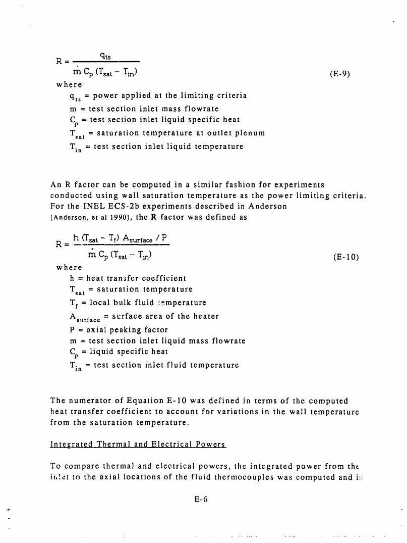
qtsR ... , ),,, .............

m Cp (Tsat - Tin) (E-9)w here

qts = power applied, at the limiting criteriam = test section inlet mass flowrate

C = test section inlet liquid specific heat

Tsat = saturation temperature at outlet plenum

Tin = test section inlet liquid temperature

An R factor can be computed in a similar fashion for experiments

conducted using wall saturation temperature as the power limiting criteria.

For the INEL ECS-2b experiments described in Anderson[Anderson, et al 1990], the R factor was defined as

h (Tsat - Tr) Asurfac o /PR ,_ -,_(1_._ ... _ i i i, ill .....

o

m Cp (Tsat - Tm) (E- 10)where

h = heat transfer coefficient

Tsa t = saturation temperature

Tf = local bulk fluid '_gmperature

msurfae e = surface area of the heater

P = axial peaking factor

m = test section inlet liquid mass flowrateC = liquid specific heatp

Tin = test section inlet fluid temperature

The numerator of Equation E-10 was defined in terms of the computed

heat transfer coefficient to account for variations in the wall temperature

from the saturation temperature•

Integrated Therm.al and Electrical Powers

']70 compare thermal and electrical powers, the integrated power from th_

inlet to the axial locations of the fluid thermocouples was computed and i:',

E-6

=

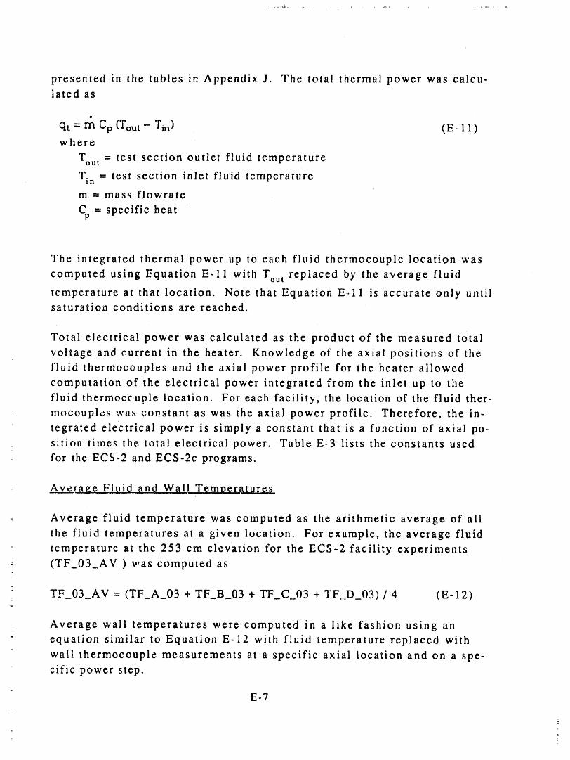
ii., LII.. , ..... ii

presented in the tables in Appendix J. The total thermal power was calcu-lated as

o

qt = m Cp(Tou t - Tin) (E-11 )where

Tou t = test section outlet fluid temperature

Tin = test section inlet fluid temperaturem = mass flowrate

C = specific heat

The integrated thermal power up to each fluid thermocouple location was

computed using Equation E-11 with Tou t replaced by the average fluid

temperature at that location. Note that Equation E-11 is accurate only untilsaturation conditions are reached.

Total electrical power was calculated as the product of the measured total

voltage and current in the heater. Knowledge of the axial positions of thefluid thermocouples and the axial power profile for the heater allowed

computation of the electrical power integrated from the inlet up to the

fluid thermocc, uple location. For each facility, the location of the fluid ther-

mocouples was constant as was the axial power profile. Therefore, the in-

tegrated electrical power is simply a constant that is a function of axial po-sition times the total electrical power. Table E-3 lists the constants used

for the ECS-2 and ECS-2c programs.

_Av,_r_age Fluid and W_II Tempe[atures

: Average fluid temperature was computed as the arithmetic average of all

the fluid temperatures at a given location. For example, the average fluid

temperature at the 253 cm elevation for the ECS-2 facility experiments

- (TF_03_AV) was computed as

o

TF_03_AV = (TF_A_03 + TF_B_03 + TF C 03 + TF.D_03) / 4 (E-12)

Average wall temperatures were computed in a like fashion using an

equation similar to Equation E-12 with fluid temperature replaced with

wall thermocouple measurements at a specific axial location and on a spe-cific power step.

E-7

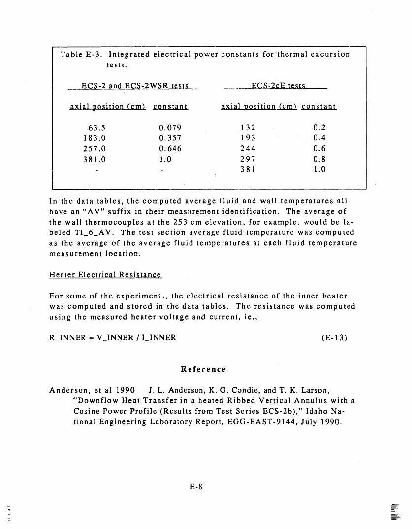
Table E-3. Integrated electrical power constants for thermal excursiontests.

ECS-2 andECS-2W$R tests . EC.S-2cE te_ts

axial position (cm) .constant. ,_xial position (cm) constant

63.5 0.079 132 0.2

183.0 0.357 193 0.4

257.0 0.646 244 0.6

381.0 1.0 297 0.8- - 381 1.0

In the data tables, the computed average fluid and wall temperatures alihave an"AV" suffix in their measurement identification. The average of

the wall thermocouples at the 253 cm elevation, for example, would be la-beled TI 6 AV. The test section average fluid temperature was computed

as the average of the average fluid temperatures at each fluid temperaturemeasurement location.

Heater Electrical Resi.Etan¢¢

For some of the experiment,,, the electrical resistance of the inner heater

was computed and stored in the data tables. The resistance was computed

using the measured heater voltage and current, ie.,

R_INNER = V_INNER / I_INNER (E- 13)

Reference

Anderson, et al 1990 J.L. Anderson, K. G. Condie, and T. K. Larson,"'Downflow Heat Transfer in a heated Ribbed Vertical Annulus with a

Cosine Power Profile (Results from Test Series ECS-2b)," Idaho Na-

tional Engineering Laboratory Report, EGG-EAST-9144, July 1990.

E-8

Appendix F

Data Repeatability for Onset of

Thermal Excursion Experiments

_r, ...... , ............. 'rtr ' p_..... n_',,n, , qp_..... r"_lll' 'mu,J_l',Ir_...... ,r,..... , p_,,,,,,..... ,a_ _ IIlq ...... It¢_, "'I_IIP lP "e'l"',_ ',,l'rer' Pl,l,Illl.......... r,, ,_pqq.... I1' I,lln,,,,l[]rl_rll',,, 'I'IT_P " _1pnrn "

,,, ,, i,,_ ,, , ,, ,,,, ,, ,,, ,,_ ,_IiI, ,_ J,, , ,_, , il,lllt , , ,il, J, Id_l t._li,,,

Appendix F

Data Repeatability for Onset of

Thermal Excursion Experiments

Data repeatability was investigated during the course of the thermal

excursion test program conducted in the ECS-2 and ECS-2b facilities by

performing essentially the same experiment multiple times. By design, the

same experiment was conducted on numerous occasions to support facility

checkout procedures, investigate changes in the facility hardware, and pro-

vide experiment/facility demonstration, s for the customer, visiting

dignitaries, and other interested personnel. A comparison of the data from

the experiments is presented in this appendix to demonstrate the high de-

gree of repeatability observed in the test results.

Thermal excursion experiment ECS-2BL_5 was conducted on four dif-ferent occasions for the reasons cited above. This test was conducted with

nominal conditions of 324 K inlet temperature, an inlet flowrate of 0.1 l/s,

and with a standpipe level of 43 cm relative to the bottom of the lower

plenum. In addition to the base case test, the experiment was also con-

ducted as ECS-2BL_5B, ECS-2BL_5C, and ECS-2BL_5D with the actual condi-tions and on the dates shown in Tab_r_ F-1.

Conduct dates for the repeatability tests are shown in the second col-

umn of Table F-1. It is noteworthy that these experiments were not ali

= conducted on the same date and that the elapsed time between perfor-

mance of the individual tests was nearly a calendar week in ali cases.Also, between the conduct of the base case test and ECS-2BL_5B, the

bottom 1.8 m of the Lexan 'rM shroud I was replaced with 1.8 m of aluminumshroud of the same inner diameter.

Examination of the values in Table F-1 shows that the variation in

flowrate and inlet temperature between the tests was less than 6% and 1%,

respectively. Such small differences influence the energy balance so that

the power required to saturate the fluid in the lower plenum (the eighth

1. During testing, the heater and shroud came in contact resulting in deformationand partial melting of the lower part of the shroud. To preclude further prob-lems, the decision was made to replace the lower part of the shroud with alumi-num.

F-1

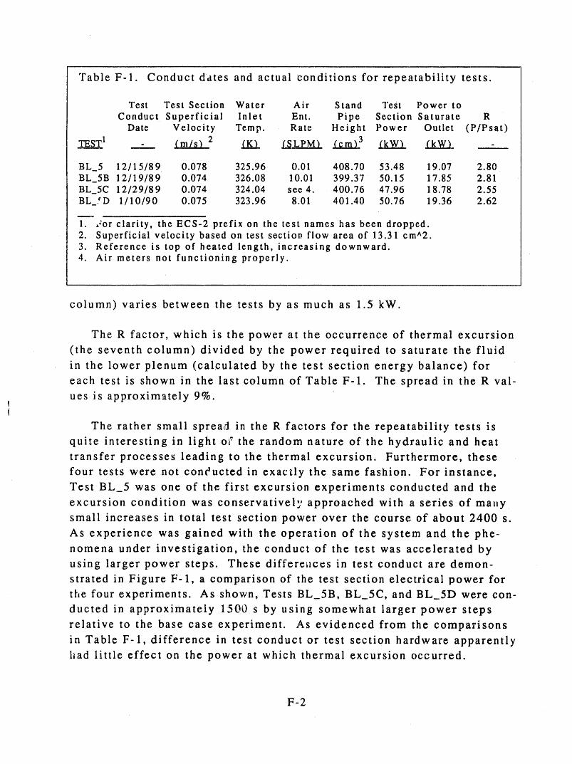
Table F-1. Conduct dates and actual conditions for repeatability tests.

Test Test Section Water Air Stand Test Power toConduct Superficial Inlet Ent. Pipe Section Saturate R

Date Velocity Temp. Rate Height Power Outlet (P/Psat)

.TEST1 - (m/s) 2 (K) .(__.LPM) .(..C,.__3. (kW) _ -

BL_5 12/15/89 0.078 325.96 0.01 408.70 53.48 19.07 2.80BL_5B 12/19/89 0.074 326.08 10.01 399.37 50.15 17,85 2.81BL 5C 12/29/89 0.074 324.04 see 4. 400.76 47.96 18.78 2.55BL_'D 1/10/90 0.075 323.96 8,01 401.40 50.76 19.36 2.62

"_"."Jor clarity, the ECS-2 prefix on the test names has been dropped.2. Superficial velocity based on test section flow area of 13.31 cm^2.3. Reference is top of heated length, increasing downward.4. Air meters not functioning properly.

column) varies between the tests by as much as 1.5 kW.

The R factor, which is the power at the occurrence of thermal excursion

(the seventh column) divided by the power required to saturate the fluid

in the lower plenum (calculated by the test section energy balance) for

each test is shown in the last column of Table F-1. The spread in the R val-

ues is approximately 9%.

The rather small spread in the R factors for the repeatability tests is

quite interesting in light o_" the random nature of the hydraulic and heat

transfer processes leading to the thermal excursion. Furthermore, these

four tests were not conducted in exactly the same fashion. For instance,

Test BL_5 was one of the first excursion experiments conducted and the

excursion condition was conservatively approached with a series of many

small increases in total test section power over the course of about 2400 s.

As experience was gained with the operation of the system and the phe-

nomena under investigation, the conduct of the test was accelerated byusing larger power steps. These differe_lces in test conduct are demon-

strated in Figure F-l, a comparison of the test section electrical power for

the four experiments. As shown, Tests BL_5B, BL_5C, and BL_5D were con-

ducted in approximately 1500 s by using somewhat larger power steps

relative to the base case experiment. As evidenced from the comparisons

in Table F-l, difference in test conduct or test section hardware apparentlylaad little effect on the power at which thermal excursion occurred.

F-2

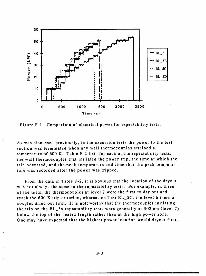
0 ' i ii

so i,tf,-,40 ..'T'lmW _i_ "-"BL_5

--" BL_5B

-= ' !1iR10 ' °

- ,_ I _ I I0 "

0 500 1000 1500 2000 2500

Time (s)

Figure F-1. Comparison of electrical power for repeatability tests.

As was discussed previously, in the excursion tests the power to the test

section was terminated when any wall thermocouples attained a

temperature of 600 K. Table F-2 lists for each of the repeatability tests,

the wall thermocouples that initiated the power trip, the time at which the

trip occurred, and the peak temperature and time that the peak tempera-

ture was recorded after the power was tripped.

From the data in Table F-2, it is obvious that the location of the dryout

was not always the same in the repeatability tests. For example, in three

of the tests, the thermocouples at level 7 were the first to dry out and

reach the 600 K trip criterion, whereas on Test BL_5C, the level 6 thermo-

couples dried out first. It is noteworthy that the thermocouples initiating

the trip on the BL_5x repeatability tests were generally at 302 cm (level 7)

below the top of the heated length rather than at the high power zone.

One may have expected that the highest power location would dryout first.

F-3

II III I

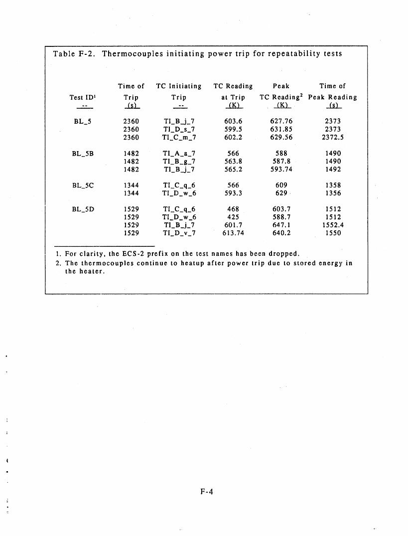
Table F-2. Thermocouples initiating power trip for repeatability tests

Time of TC Initiating TC Reading Peak Time of

Test ID _ Trip Trip at Trip TC Reading s Peak Reading-- _1_ -- _ K..I.._2_

BL_5 2360 TI_B..j_7 603.6 627.76 23732360 TI_D_s_7 599.5 631.85 23732360 TI_C_m_7 602,2 629.56 2372.5

BL_SB 1482 TI_A_a_7 566 588 14901482 TI_B_g_7 563.8 587.8 14901482 TI_B_.j_7 565.2 593 .'74 1492

BL5C 1344 TI_C_q_6 566 609 13581344 TI_D_ w_6 593.3 629 1356

BL_5D 1529 TI._C_q_6 468 603.7 15121529 TID w 6 425 588.7 15121529 TI_B_j_7 601.7 647.1 1552.41529 TI D v 7 613.74 640.2 1550

1. For clarity, the ECS-2 prefix on the test names has been dropped.

2. The thermocouples continue to heatup after power trip due to stored energy inthe heater.

F-4

i

Appendix G

ECS-2 Air Ingress Test Results

Appendix G

ECS-2 Air Ingress Test Results

INTRODUCTION

Twelve experiments were conducted in the ECS-2 facility to examine

the functionalrelationship between the rate at which air was entrained

into the test section and other test section boundary conditions. These ex-

periments were termed the air ingress (AI) tests. Inlet liquid temperature,,

and flowrate and back pressure on the lower plenum (the standpipe

setting) were the major variables in the AI tests.

The procedure used to conduct the AI tests was somewhat different

than the procedure used to conduct the excursion tests. Since the major

objective of the AI tests was to determine the parameters influencing en-trainment of air into the test section, the heater was not energized. For a

given standpipe setting and inlet fluid temperature, experiment conduct

entailed injecting water into the upper plenum in the normal manner,

allowing the test section to stabilize, printing a data scan (an average of

approximately 25 seconds of data) on the DAS, and then changing the inlet

liquid flowrate and repeating the data scan. For the AI tests, the inlet liq-uid flowrate was increased in 0.2 1/s increments between 0.1 and 1.5 l/s.

After a change in inlet flowrate, the test section was allowed tostabilize

for at least 2 minutes before taking a data scan.

Tests were conducted with three different inlet temperatures and four

= different standpipe settings. Table G-1 is the test matrix for the AI test

group.

RESULTS

Data collected during the AI test series shows that, for a given stand-

. pipe level _ and inlet liquid temperature, the rate at which air is entrained

into the top of the test section increases with increasing liquid flowrate.

Figures G-I, Go2, and G-3 graphically present the data collected during the

: 1. For the purposes of this discussion, the standpipe level is referenced to the bottomof the lower plenum.

G-1

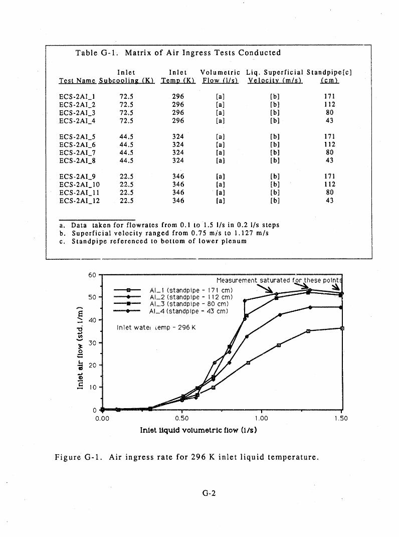
Table G-1. Matrix of Air Ingress Tests Conducted

Inlet Inlet Volumetric Liq. Superficial Standpipe[c]Test Nclme Subcooling (KL T_mp (K) Flow (l/s) .Velocity (m/s_ (cm_

ECS-2AI_I 72.5 296 [ai [bi 171ECS-2AI_2 72.5 296 la] [b] 112ECS-2AI_3 72.5 296 [ai [bi 80ECS -2AI_4 72.5 296 [ai [bi 43

ECS-2AI_5 44.5 324 [ai [bi 171ECS-2AI_6 44.5 324 [ai [bi 112ECS-2AI_7 44.5 324 [ai [bi 80ECS -2AI_8 44.5 324 [ai [bi 43

ECS-2AI_9 22.5 346 [ai [bi 171ECS-2AI_10 22.5 346 [ai [bi 112ECS-2AI_I 1 22.5 346 [ai [bi 80ECS-2AI_12 22.5 346 la] [bi 43

a. Data taken for flowrates from 0.1 to 1.5 l/s in 0.2 l/s stepsb. Superficial velocity ranged from 0.75 mis to 1.127 m/sc. Standpipe referenced to bottom of lower plenum

60Measurement saturated f.or.these point.'

ii_ AI_I (standpipe - 171 cm) _ w

50 ., A AI_2 (standpipe I12 cm) ._.-.--"_-_l -'-_'_ --1.-. AI_3 (standpipe 80 cm) 1" _7 _-1_ AI_4 (standpipe 43 cre) _Id1_ f

40

Inletwatei _emp-296K

" 30

N 2o

0 " --'=m " -- ' I " I "-

0.00 0.50 1.00 1.50

Inlettlquldvolumetric flow (I/s)

Figure G-1. Air ingress rate for 296 K inlet liquid temperature.

G..2

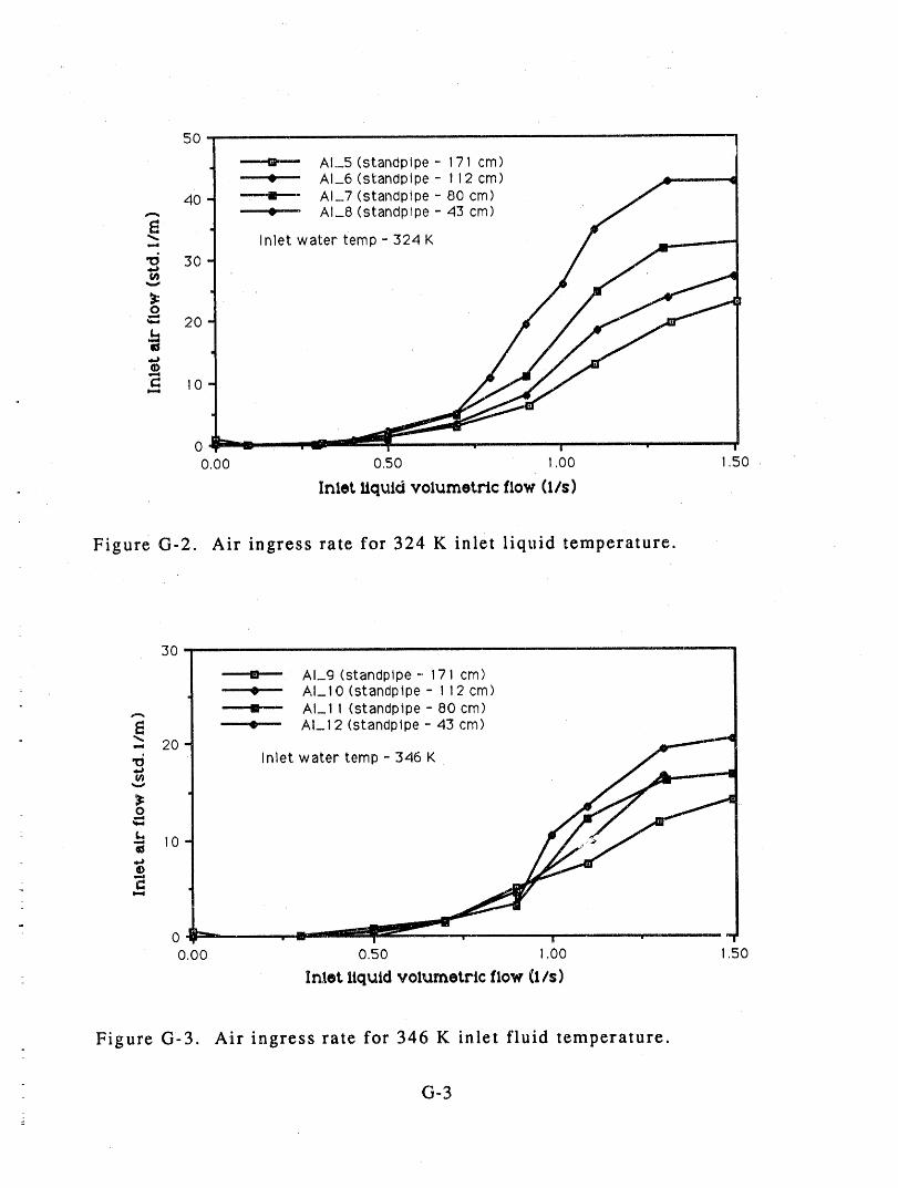
5O

Al_5(standpipe - 171 cm)¢, AI_6 (standpipe - 112 cm)

40 ----,Iii-- AI_7 (standpipe - 80 cre)- AI_8 (standpipe - 43 cre)

Inlet water temp - 324 K_ 3O

O_ 20

a

lD

_ lO_ ,

0o.oo o,5o 1,oo 1,5o

InletUquid volumetric flow (I/s)

Figure G-2. Air ingress rate for 324 K inlet liquid temperature.

30 __-i-

I_ ¢- AI_I 2 (standpipe - 43 cm).i. 20

Inlet water temp - 346 K

O

-. l0

0o.oo o.so 1.oo 1.5o

Inlet liquid volumetric flow (1/s)

Figure G-3. Air ingress rate for 346 K inlet fluid temperature.

G-3

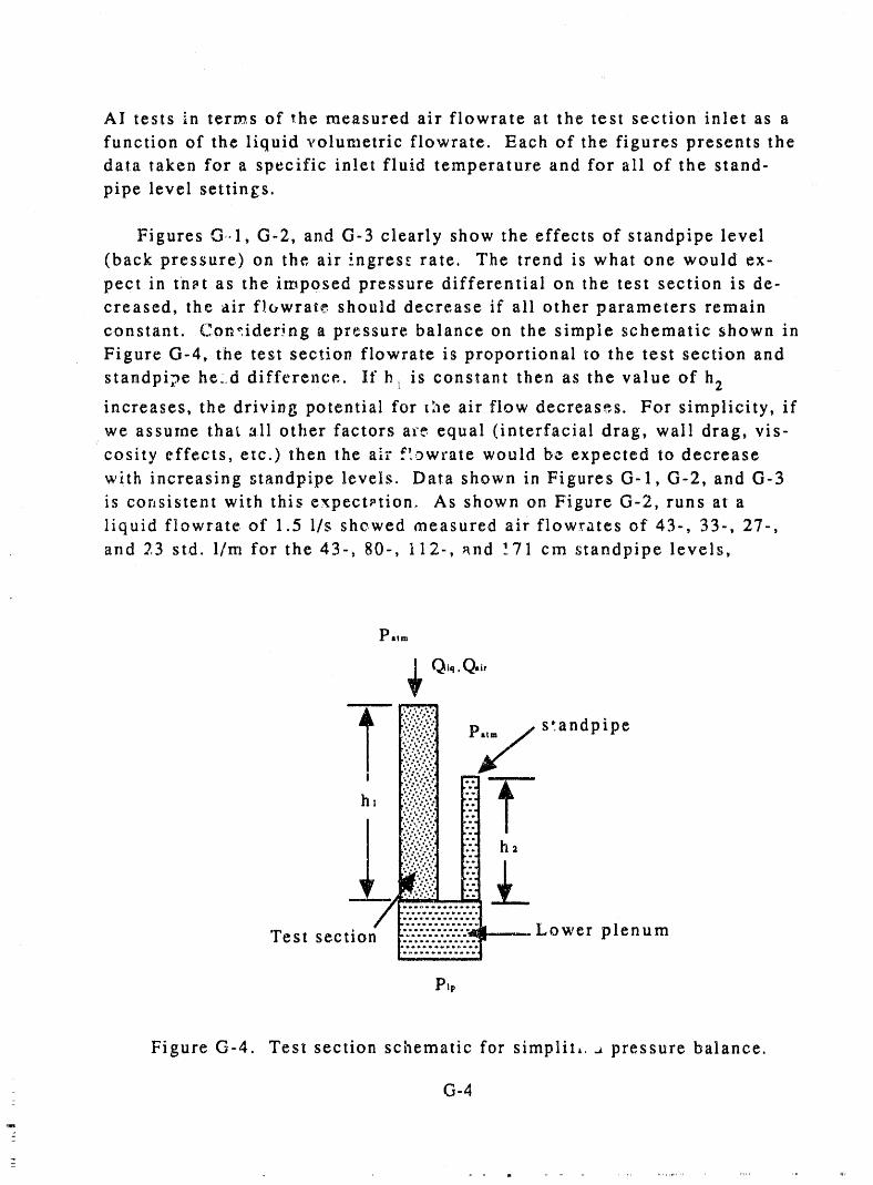
AI tests in terms of the measured air flowrate at the test section inlet as a

function of the liquid volumetric flowrate. Each of the figures presents thedata taken for a specific inlet fluid temperature and for ali of the stand-

pipe level settings.

Figures G,.1, G-2, and G-3 clearly show the effects of standpipe level

(back pressure)on the air ingress rate. The trend is what one would ex-

pect in that as the imposed pressure differential on the test section is de-

creased, the air flowrate should decrease if ali other parameters remain

constant. Con-idering a pressure balance on the simple schematic shown in

Figure G-4, the test section flowrate is proportional to the test section and

standpipe he..d difference. If b t is constant then as the value of h 2

increases, the driving potential for the air flow decreases. For simplicity, if

we assume that z ll other factors a_'e equal (interfacial drag, wall drag, vis-

cosity effects, etc.) then the air ¢'9.., wrate would be expected to decrease

with increasing standpipe levels. Data shown in Figures G-l, G-2, and G-3

is consistent with this expectation. As shown on Figure G-2, runs at a

liquid flowrate of 1.5 1/s shewed measured air flowrates of 43-, 33-, 27-,

and 23 std. 1/m for the 43-, 80-, I12-, and !71 cna standpipe levels,

Figure G-4. Test section schematic for simplit,,., pressure balance.

G-4

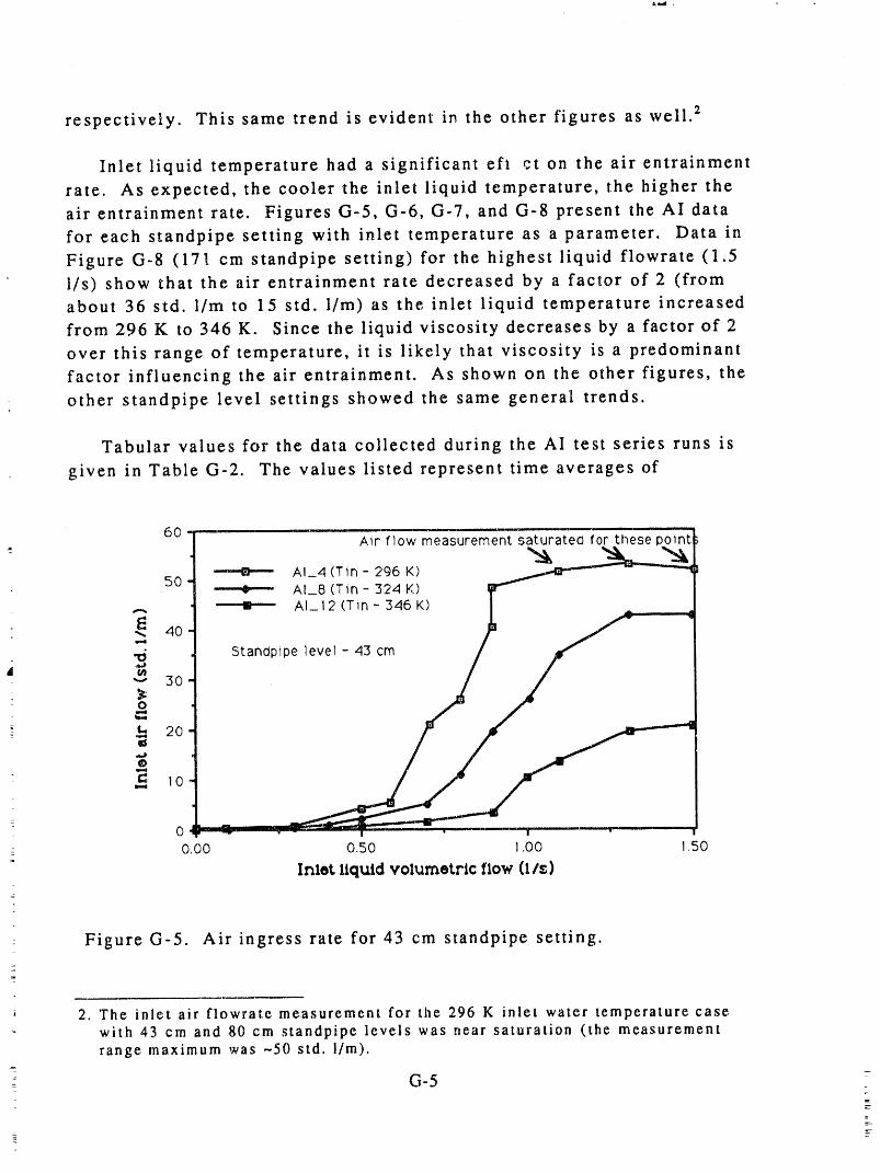
respectively. This same trend is evident in the other figures as well. 2

Inlet liquid temperature had a significant efl ct on the air entrainment

rate. As expected, the cooler the inlet liquid temperature, the higher the

air entrainment rate. Figures G-5, G-6, G-7, and G-8 present the AI data

for each standpipe setting with inlet temperature as a parameter. Data in

Figure G-8 (171 cm standpipe setting) for the highest liquid flowrate (1.5l/s) show that the air entrainment rate decreased by a factor of 2 (fromabout 36 std. l/m to 15 std. l/m) as the inlet liquid temperature increased

from 296 K to 346 K. Since the liquid viscosity decreases by a factor of 2

over this range of temperature, it is likely that viscosity is a predominant

factor influencing the air entrainment. As shown on the other figures, the

other standpipe level settings showed the same general trends.

Tabular values for the data collected during the AI test series runs is

given in Table G-2. The values listed represent time averages of

60 -- Air flow measurement saturated for these pointl_

50 _ AI__4 (Tin- 296 K)AI_8 (Tin - 324 K) _ I

"_1_ 40 _ AI._12(Tin- 346K) /_ J ...... ii,_ Standpipe level - 43 cm

d m'_ 30

" ,,.,"_ , _ _.

_- _ 20

@

IIIl

z

-- -- i i iit •I

- o.oo 050 l,oo 1.5o

Inlot liquid volumetric flow (l/s)

Figure G-5. Air ingress rate for 43 cm standpipe setting.

2. The inlet air flowrate measurement for the 296 K inlet water temperature case

with 43 cm and 80 cm standpipe levels was r_ear saturation (the measurementrange maximum was --50 std. l/m).

=

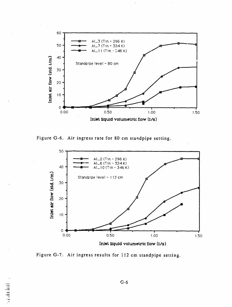
60 i._.--- : III I

AI_3 (Tin - 296 K) _.....4_i.-_J50 _, AI_7 (Tin- 324 K) /l"_-- _ I

_'1_ 40 -I'-Ii-I" Al_ 11 (t in '":.46 K) f_" I.,_ Standpipe level - 80 cm

30

•- 20

-' 10o

0 ! I

0.00 0.50 ! .00 1.50

Inlet Uquld voltametre flow (IIs)

Figure G-6. Air ingress rate for 80 cm standpipe setting.

50

AI_2 (Tin - 296 K)AI_6 (Tin - 324 K)

40 "-"ii-'- AI_lO (Tin - 346 K)

Standpipe level - i12 cml.III

•_i 3o

0•-' 20

a

o

0

o.oo 050 l.oo 1.5o

Inlet Uquld volumet_c flow (lls)

Figure G-7. Air ingress results for 112 cm standpipe setting.

iz_=

I

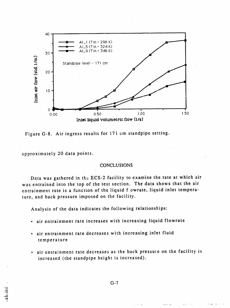
40 _

AI_I (Tin- 296 K)¢. - AI_5 (Tin - 324 K)

.-._ 30 ---Ii-I---- AI_9 (Tin - 346 K) _/

_" Standpipe level-- 171 cm / ,/20

_ 10,_,,_

0 io.oo o.5o I,oo 1.5o

Inlot Uquld volum_trlc flow (l/s)

Figure G-8. Air ingress results for 171 cm standpipe setting.

approximately 20 data points.

CONCLUSIONS

Data was gathered in tE; ECS-2 facility to examine the rate at which air

was entrained into the top of the test section. The data shows that the air

entrainment rate is a function of the liquid f, owrate, liquid inlet tempera-

ture, and back pressure imposed on the facility.

Analysis of the data indicates the following relationships"

• air entrainment rate increases with increasing liquid flowrate

• air entrainment rate decreases with increasing inlet fluid

temperature

° air entrainment rate decreases as the back pressule on the facility is

increased (the standpipe height is increased).

G-7

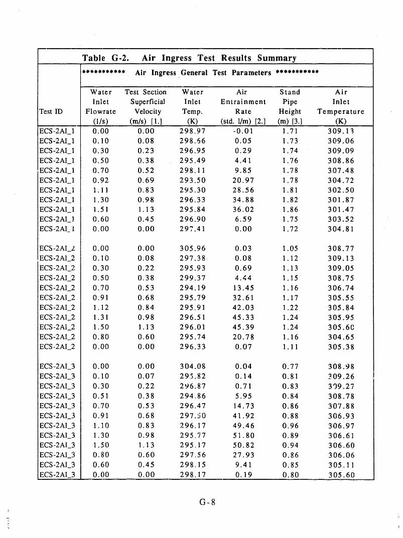
Table G.2. Air Ingress Test Results Summary

*********** Air Ingress General Test Parameters ***********

Water Test Section Water Air Stand Air

Inlet Superficial Inlet Entrainment Pipe Inlet

Test ID Flowrate Velocity Temp. Rate Height Temperature

(l/s) (m/s) [1.] (K) (std. l/m) [2.] (m) [3.] (K)ECS-2AI_I 0.00 0.00 298,97 -0.01 1.71 309.13

ECS-2AI_I 0.10 0.08 298 56 0.05 1.73 309.06

ECS-2AI_I 0.30 0.23 296 95 0.29 1.74 309.09

ECS-2AI_I 0.50 0.38 295 49 4.41 1.76 308.86

ECS-2AI_I 0.70 0.52 298 11 9.85 1 78 307.48

ECS-2AI 1 0.92 0.69 293 50 20.97 1 78 304.72

ECS-2AI_I 1.11 0.83 295 30 28.56 1 81 302,50

ECS-2AI_I 1.30 0.98 296 33 34.88 1 82 301.87

ECS-2AI_I 1.51 1.13 295 84 36.02 1 86 301.47

ECS-2AI__ 0.60 0.45 296 90 6.59 1 75 303.52

ECS-2AI_I 0.00 0.00 297 41 0.00 1 72 304.81

ECS-2AI_2 0.00 0.00 305 96 0.03 1 05 308.77

ECS-2AI_2 0 10 0.08 297 38 0.08 1 12 309.13

ECS-2AI_2 0 30 0.22 295 93 0.69 1 13 309.05

ECS-2AI_2 0 50 0.38 299.37 4.44 1 15 308.75

ECS-2AI_2 0.70 0.53 294 19 13.45 1 16 306.74

ECS-2AI_2 0.91 0.68 295 79 32.61 1 17 305.55

ECS-2AI_2 1 12 0.84 295 91 42.03 1 22 305.84

ECS-2AI 2 1 31 0.98 296 51 45.33 1 24 305.95

ECS-2AI 2 1 50 1.13 296 01 45.39 1 24 305.60

ECS-2AI_2 0 80 0.60 295 74 20.78 1 16 304.65

ECS-.2AI_2 0.00 0.00 296 33 0.07 1 11 305.38

ECS-2AI_3 0 00 0.00 304 08 0.04 0.77 308.98

ECS-2AI_3 0 10 0.07 29,5 82 0.14 0.81 309.26

ECS-2AI_3 0 30 0.22 296 87 0.71 0.83 399.27

ECS-2AI_3 0 51 0.38 294 86 5.95 0.84 308.78

ECS-2AI_3 0 70 0.53 296 47 14.73 0.86 307.88

ECS-2AI_3 0 91 0.68 297 50 41.92 0.88 306 93

ECS-2AI_3 1 10 0.83 296 17 49.46 0.96 306 97

ECS-2AI_3 1 30 0.98 295 77 51.80 0.89 306 61

ECS-2AI_3 1 50 1.13 295 17 50.82 0 94 306 60

ECS-2AI 3 0 80 0.60 297.56 27.93 0 86 306 06

ECS-2AI_3 0 60 0.45 298.15 9.41 0 85 305 11

ECS-2AI_3 0 00 0.00 298.17 0.19 0 80 305.60

G-8

L

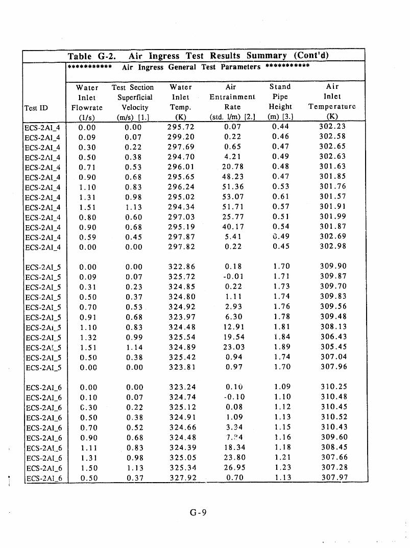
Table G-2. Air Ingress Test Results Summary (Cont'd)*********** Air Ingress General Test Parameters ***********

" Water Test Section Water Air Stand Air

Inlet Superficial Inlet Entrainment Pipe InletTest ID Flowrate Velocity Temp. Rate Height Temperature

(l/s) (m/s) [1.] (K) (std. l/m) [2.] (m) [3.] (K)

ECS-2AI_4 0.00 0.00 295.72 0 07 0.44 302.23

ECS-2AI._4 0,09 0.07 299.20 0 22 0.46 302.58

ECS-2AI_4 0.30 0.22 297,69 0 65 0.47 302.65

ECS-2AI._4 0.50 0.38 294.70 4.21 0.49 302.63

ECS-2AI_4 0.71 0.53 296.01 20 78 0.48 301.63

ECS-2AI_4 0.90 0.68 295.65 48 23 0.47 301.85

ECS-2AI._4 1.10 0.83 296.24 51.36 0.53 301.76

ECS-2AI_.4 1.31 0.98 295 02 53.07 0.61 301.57

ECS-2AI_4 1.51 1.13 294 34 51.71 0.57 301.91

ECS-2AI 4 0.80 0.60 297 03 25.77 0 51 301.99

ECS-2AI_4 0.90 0,68 295 19 40.17 0 54 301.87

ECS-2AI_4 0.59 0.45 297 87 5.41 0 49 302.69

ECS-2AI_4 0.00 0.00 297 82 0.22 0.45 302.98

ECS-2AI_5 0.00 0.00 322.86 0.18 1.70 309.90

ECS-2AI_5 0.09 0.07 325.72 -0.01 1.71 309.87

ECS-2AI_5 0.31 0.23 324.85 0.22 1.73 309.70

ECS-2AI_5 0.50 0.37 324.80 1.11 1.74 309.83

ECS-2AI_5 0.70 0.53 324.92 2.93 1.76 309.56

ECS-2AI_5 0.91 0.68 323.97 6.30 1 78 309.48

ECS-2AL.5 1.10 0.83 324.48 12.91 1 81 308.13

ECS-2AI. 5 1.32 0.99 325.54 19.54 1 84 306.43

ECS-2Ar,_5 1.51 1.14 324.89 23.03 1 89 305 45

ECS-2AI_5 0.50 0.38 325.42 0.94 1 74 307.04

ECS-2AI_5 0.00 0.00 323.81 0.97 1 70 307.96

ECS-2AI_6 0.00 0.00 323.24 0.10 1.09 310.25

ECS-2AI 6 0.10 0.07 324.74 -0.10 1.10 310.48

ECS-2AI_6 G.30 0.22 325.12 0.08 1.12 310.45

ECS-2AI_6 0.50 0.38 324.91 1.09 1.13 310.52

ECS-2AI_6 0.70 0.52 324.66 3.34 1 15 310.43

ECS-2AI_6 0.90 0.68 324.48 7._!4 1 16 309.60

ECS-2AI 6 1.11 0.83 324.39 18.34 1 18 308.45

ECS-2AI_6 1.31 0.98 325.05 23.80 1 21 307.66

ECS-2AI_6 1.50 1.13 325.34 26.95 1 23 307.28

ECS-2AI_6 0.50 0.37 327.92 0.70 1 13 307.97

G-9

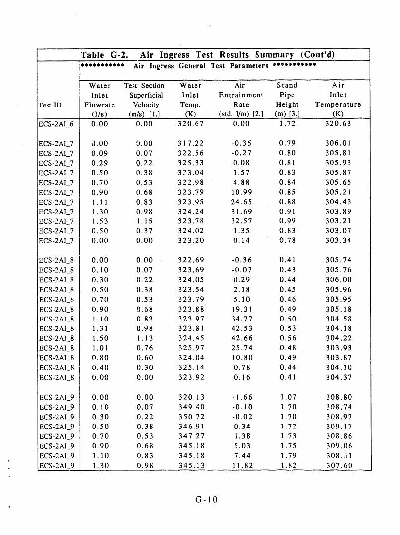
Table G.2. Air Ingress Test Results Summary. (Cont'd).,*********** Air Ingress General Tesf"'Parameters **_********

, ,,

Water Test Section Water Air Stand Air

Inlet Superficial Inlet Entrainment Pipe Inlet

Test lD Flowrate Velocity Temp. Rate Height Temperature

(l/s) (m/s) [1.l (K) (st d. l/m) [2.l (m) [3.1 (K)ECS-2AI_6 0.00 0.00 320.67 0.00 1.72 320.63

ECS-2AI_7 O.00 9.00 317.22 -0.35 0.79 306.01

ECS-2AI_7 0.09 0.07 322.56 -0.27 0.80 305.81

ECS-2AI_7 0.29 0.22 325.33 0.08 0.81 305.93

ECS-2AI_7 0.50 0.38 323.04 1.57 0.83 305.87

ECS-2AI_7 0.70 0.53 322.98 4.88 0.84 305.65

ECS-2AI,7 0.90 0,68 323.79 10.99 0.85 305.21

ECS-2AI_7 1.11 0.83 323.95 24.65 0.88 304.43

ECS-2AI_7 1.30 0.98 324.24 31.69 0.91 303.89

ECS-2AI_7 1.53 1.15 323.78 32.57 0.99 303.21

ECS-2AI_7 0.50 0.37 324.02 1.35 0.83 303.07

ECS-2AI_7 0.00 0100 323.20 0.14 0.78 303.34

ECS-2AI_8 0.00 0.00 322.69 -0.36 0.41 305.74

ECS-2AI_8 0.10 0.07 323.69 -0.07 0.43 305.76

ECS-2AI_8 0.30 0.22 324.05 0.29 0.44 306.00

ECS-2AI_8 0.50 0.38 323.54 2.18 0.45 305.96

ECS-2AI._8 0.70 0.53 323.79 5.10 0.46 305.95

ECS-2AI_8 0.90 0.68 323.88 19.31 0.49 305.18

ECS-2AI_8 1.10 0.83 323.97 34.77 0.50 304..58

ECS-2AI_8 1.31 0.98 323.81 42.53 0.53 304.18

ECS-2AI_8 1.50 1.13 324.45 42.66 0.56 304.22

ECS-2AI_8 1.01 0.76 325.97 25,74 0.48 303.93

ECS-2AI_8 0.80 0.60 324.04 10.80 0.49 303.87

ECS-2AI_8 0.40 0.30 325.14 0.78 0.44 304.10

!ECS-2AI_.8 0.00 0.00 323.92 0.16 0.41 304.37

ECS-2AI_9 0.00 0.00 320.13 -1.66 1.07 308.80

ECS-2AI_9 0.10 0.07 349.40 -0.10 1.70 308.74

ECS-2AI_9 0.30 0.22 350.72 -0,02 1.70 308.97

ECS-2AI_9 0.50 0.38 346.91 0.34 1.72 309.17

ECS-2AI_9 0.70 0.53 347.27 1.38 1.73 308.86

ECS-2AI_9 0.90 0.68 345.18 5.03 1.75 309.06

ECS-2AI_9 1.10 0.83 345.18 7.44 1.79 308.51

. ECS-2AI_9 1.30 0.98 34_5. !3 11_.82 ___ 1.82 30_7.60

G-lO

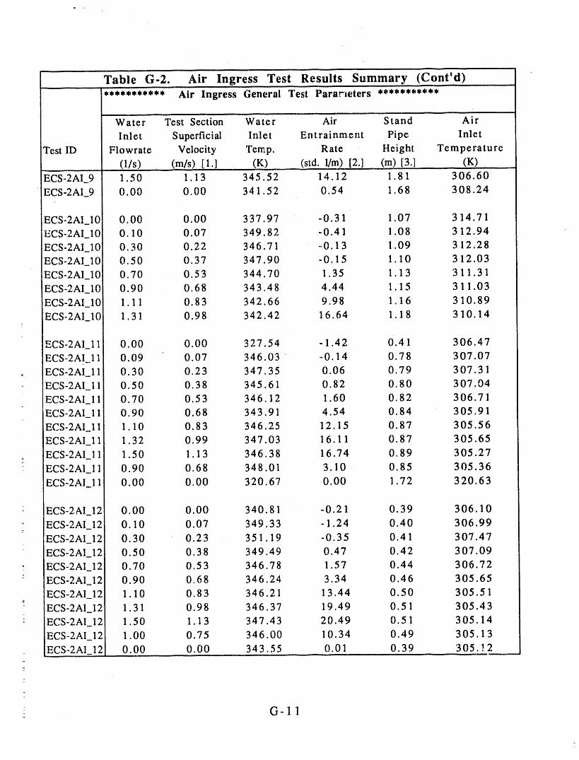
..... Table G-2. Air Ingress Test Results Summary (C,.ont'd)*********** Air Ingress General Test Para_leters ***********

, ,,, ,, ,

water TeSt Section Water Air Stand Air

Inlet Superficial Inlet Entrainment Pipe InletTest ID Flowrate Velocity Temp. Rate Height Temperature

(l/s) (m/s) [1.1 (K) (std. l/m) [2.1 (m) [3.] (K)ECS-2AI_9 1.50 1.13 345.52 14.12 1.81 306.60

ECS-2AI_9 0.00 0.00 341.52 0.54 1.68 308.24

ECS-2AI_10 0.00 0.00 337.97 -0.31 1.07 314.71

ECS-2AI_10 0.10 0,07 349.82 -0.41 1.08 312.94

ECS-2AI_10 0.30 0.22 346.71 -0.13 1.09 312.28

ECS-2AI_10 0.50 0.37 347.90 -0.15 1.10 312.03

ECS-2AI_10 0.70 0.53 344.70 1.35 1.13 311,31

ECS-2AI_10 0.90 0.68 343.48 4.44 1.15 311.03

ECS-2AI_10 1.11 0,8,3 342.66 9.98 1.16 310.89

ECS-2AI_10 1.31 0.98 342,42 16.64 1.18 310.14

ECS-2AI_ll 0.00 0.00 327.54 -1.42 0.41 306.47

ECS-2AI_.I 1 0.09 0.07 346.03 -0.14 0.78 307.07

ECS-2AI_I 1 0.30 0.23 347.35 0.06 0.79 307.31

ECS-2AI_I 1 0,50 0.38 345.61 0.82 0.80 307.94

ECS-2AI_I 1 0.70 0.53 346.12 1.60 0.82 306.71

iECS-2AI_I 1 0.90 0.68 343.91 4.54 0.84 305.91

ECS-2AI_I 1 1.10 0.83 346.25 12.15 0.87 305.56

ECS-2AI_ll 1,32 0.99 347.03 16.11 0.87 305.65

o ECS-2AI_I 1 1.50 1.13 346,38 16.74 0.89 305.27

ECS-2AI_I 1 0.90 0.68 348.01 3.10 0.85 305.36

ECS-2AI_I 1 0.00 0.00 320.67 0.00 1.72 320.63

ECS-2AI_12 0.00 0.00 340.81 -0.21 0.39 306.10

ECS-2AI_12 0.10 0.07 349.33 -1.24 0.40 306.99

ECS-2AI 12 0.30 0.23 351.19 -0.35 0.41 307.47

ECS-2AI_12 0.50 0.38 349.49 0.47 0.42 307.09

- ECS-2AI_12 0.70 0.53 346.78 1.57 0.44 306.72

ECS-2AI_12 0.90 0.68 346.24 3.34 0.46 305.65

ECS-2AI_12 1.10 0.83 346.21 13.44 0.50 305.51

-- :ECS-2AI_12 1.31 0.98 346.37 19.49 0.51 305.43

ECS-2AI_12 1.50 1.13 347.43 20.49 0.51 305,14

ECS-2AI_12 1.00 0.75 346.00 10.34 0.49 305.13

ECS-2AI_12 0.00 0.00 343.55 0.01 ..... 0.39 305.,12

- G-11

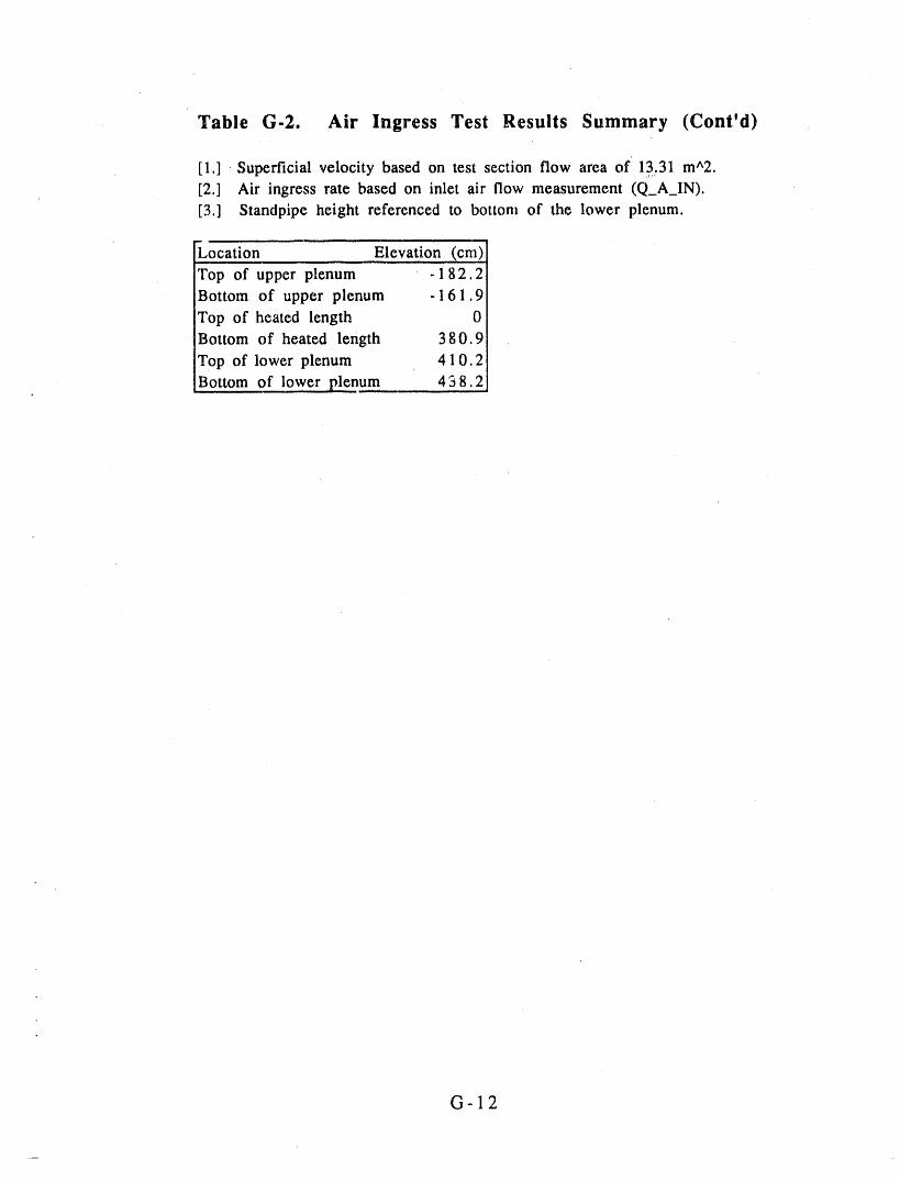
Table G-2. Air Ingress Test Results Summary (Cont'd)

[1.] Superficial velocity based on test section flow area of 13:31 m^2.[2.] Air ingress rate based on inlet air flow measurement (Q_A_IN).

[3.] Standpipe height referenced to bottom of the lower plenum.

Location Elevation (cre)

Top of upper plenum - 182.2

Bottom of upper plenum - 161.9

Top of heated length 0Bottom of heated length 380.9

Top of lower plenum 410.2

Bottom of lower p.]enum 438.2

G-12

Appendix H

Video System Used Duringthe ECSc2 Thermal Excursion Tests

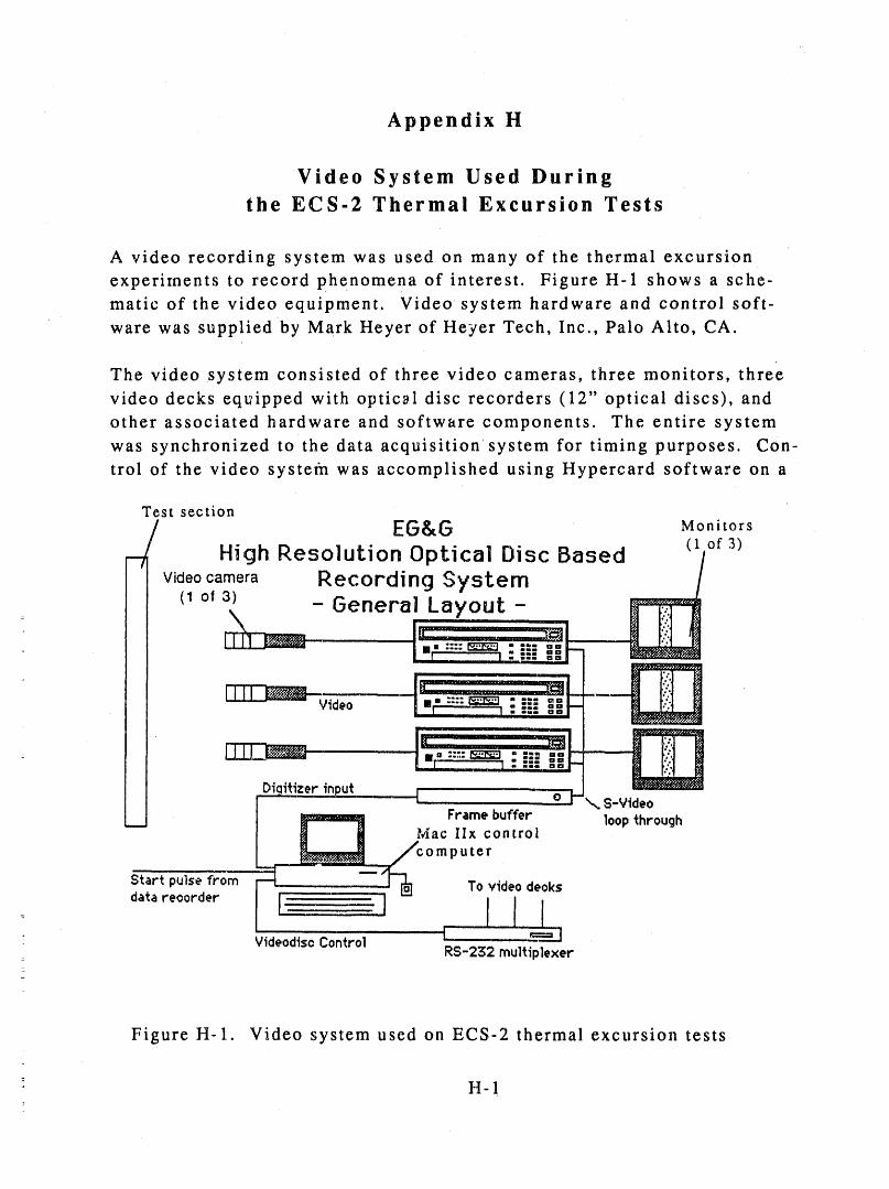
Appendix H

Video System Used Duringthe ECS-2 Thermal Excursion Tests

A video recording system was used on many of the thermal excursion

experiments to record phenomena of interest. Figure H-1 shows a sche-

matic of the video equipment. Video system hardware and control soft-

ware was supplied by Mark Heyer of Heyer Tech, Inc., Palo Alto, CA.

The video system consisted of three video cameras, three monitors, three

video decks equipped with optical disc recorders (12" optical discs), and

other associated hardware and software components. The entire system

was synchronized to the data acquisitionsystem for timing purposes. Con-

trol of the video systefn was accomplished using Hypercard software on a

Test section

/ EG_t_ Monitors(1 of 3)-/ High Resolution Optical Disc Based /

Video camera Recording System /

(1o,3) - Genera|Layout._ - :'_ ....

: LL.LL._._,_ Im_'::: _ :":=: **gii M1 F:6| !_' - , , ::: *-i-7

Di, !,u, _ ].j\ s_vtd,o,._..,,-_--- Frame buffer loopthrough

Mac IIx controlomputer

Start pulse from To video decks

: VideodJsoControl l ...... -: R5-232 multiplexer

Figure H-1. Video system used on ECS-2 thermal excursion tests

H-1

Macintosh IIx computer. Table H-1 lists the components in the video sys-tem.

The video system was capable of recording up to approximately 30 frames

per second from each of the cameras. The signal was displayed on the

monitors and/or written to optical disc for archiva!. Information regarding

the archived recordings is stored in a Hypercard stack for post-test re-

trieval/display and analysis. At the highest recording rate, each video disc

could hold approximately 30 minutes of video dat_.

For the ECS-2 and WSR tests, the top and middle camera were generallytrained on the test section high power zone (between 200- and 302 cm)

and the bottom camera was trained on the outlet plenum. Cameras were

set up to provide a 20-40 cm field of view. The system was used to moni-: tor the test section on nearly ali of the experiments although, due to the

large volume of data generated by video, video data was not archived for

ali tests nor was data archived for the whole duration of any single test.

Analysis and review of the video data is a time consuming operation. Use-

ful and informative insights can be obtained from analysis of the video

data. However, due to time constraints, video results are not presentedhere.

m

H-2

Table H-1. Video recording system components

Comt_enent Manufacturer_ Model Number

Hardware

Camera (3) (3CD TK-66

Monitor (3) Sony PVM-122

Optical Disc Recorder (3) Panasonic TQ-3031F

Optical Disc Panasonic TQ-FH331/TQ-FH3321

Video Distribution Amp. Sigma Electronics VDA-100AData Broadcast Unit Black Box DB 8/25

Digital Time BaseCorrector FOR-A FA300

Hardware/software conti'ol

Computer Apple Mac IIxController IoTech Mac/IEEE488

: I/O National Inst. NB-D10-24

Image capture SCION Image Capture 2

1. Single-sided and double-sided discs respectively.

i

" III _ rl I _ ..... Itt+lll ..... tl ,,,,, , 'qPlrr"_'........ r_1'Ir r'Irli'lllllltr H'III_" _rlll_lll,tllrl,l ii+ ,,ii,,,

A ppendix I

Questionable or Failed Measurements for theECS-2 and ECS.2cThermal Excursion Experiments,

Appendix I

Questionable or Failed Measurements for the

ECS-2 and ECS-2c Thermal Excursion Experiments

,During the INEL thermal excursion experiment program, a detailed written

log was maintained to document various aspects of the experiment includ-

ing instrumentation/measurement problems. After review of quick look

plots (data comparisons compiled immediately after the conduct of an ex-

periment) and more thorough analyses of the experimental data, additional

measurements known or suspected of being bad have been identified.

For historical documentation, the measurements known to be questionable

for each thermal excursion experiment are listed in Table I-1. The table

lists the experiment name, the date the experiment was conducted, and the

measurements identified by "DAS Tag ID" (see Appendix B for a descrip-

tion of the measurement) deemed or known to be questionable. An entry

of a particular measurement on a given test does not necessarily implythat the measurement was unusable for the whole experiment and does

not imply that the measurement was unusable for experiments conducted

chronologically after that point in time. Generally, measurements prob-lems were electrical or electronic in nature (bad connectors, problems with

analog..to-digital conversion cards, broken wires, reference oven problems,

etc.) and were readily corrected once identified.

The information in Table I-1 provides a quick indication of measurements

that obviously experienced some problem during the excursion tests and

does not constitute an extensive data quality review. Furthermore, the

fact that an instrument is not listed in the table does not guarantee that

the measurement performed flawlessly during the experiments.

I-1

Q

_ I I I I I I I I I I

m

0o0

m

m

c

Co

E_ _1 I I ! I I 6_1 I t I

, _ "ml I I I I ..li

- ' & m & & m u_

_

_7-2

II I_ l@ II llllll'lll lI I'll l rpl ' l l !li l l'(ll ' lrM' 1[11 l_ l l 'l I l l rl])lllllll'll lllIlll_ llll lm r_ l[tllllll .....

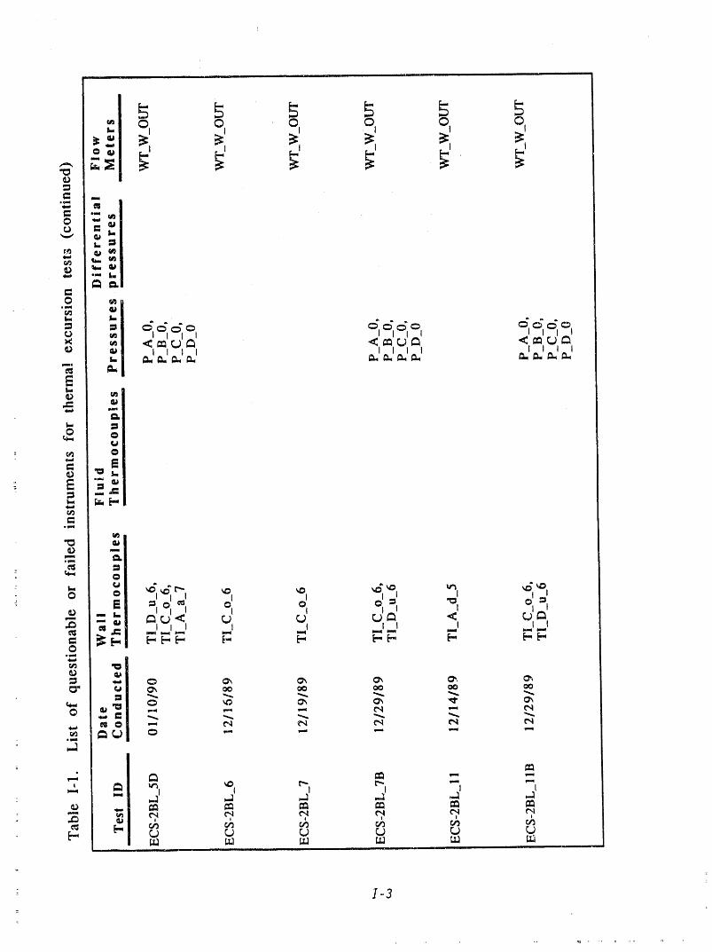
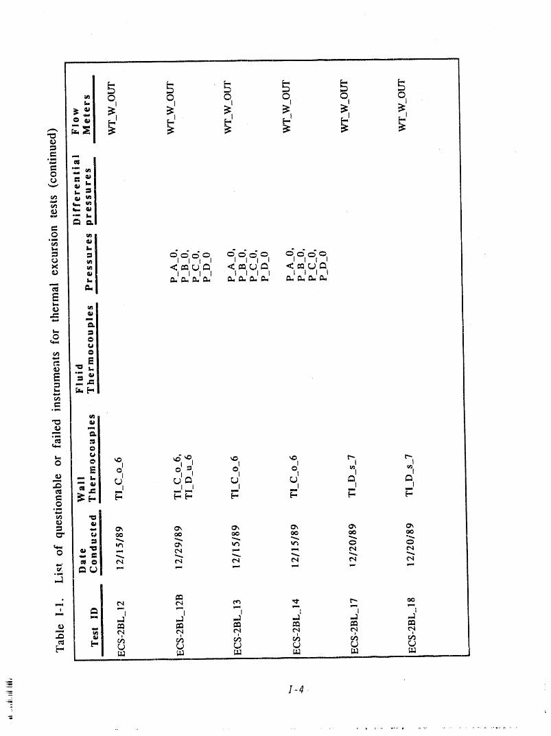
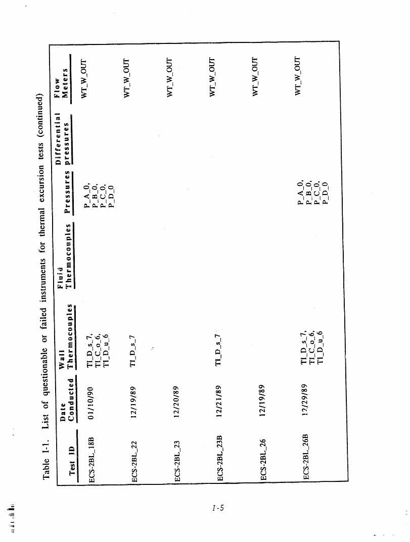
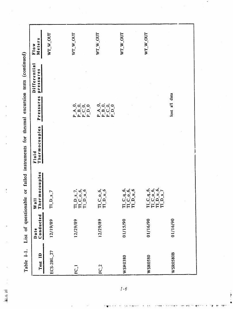
!-G

" _li'l' " ...... IIII ""'_l_,il I' _'_,. ' iri H,-l'i . _.' _,,,,,,l,,plpWi1,11r _H H[,,11,1'ri _ ,,, ,, 'i_, i_q, i11!11e,,r

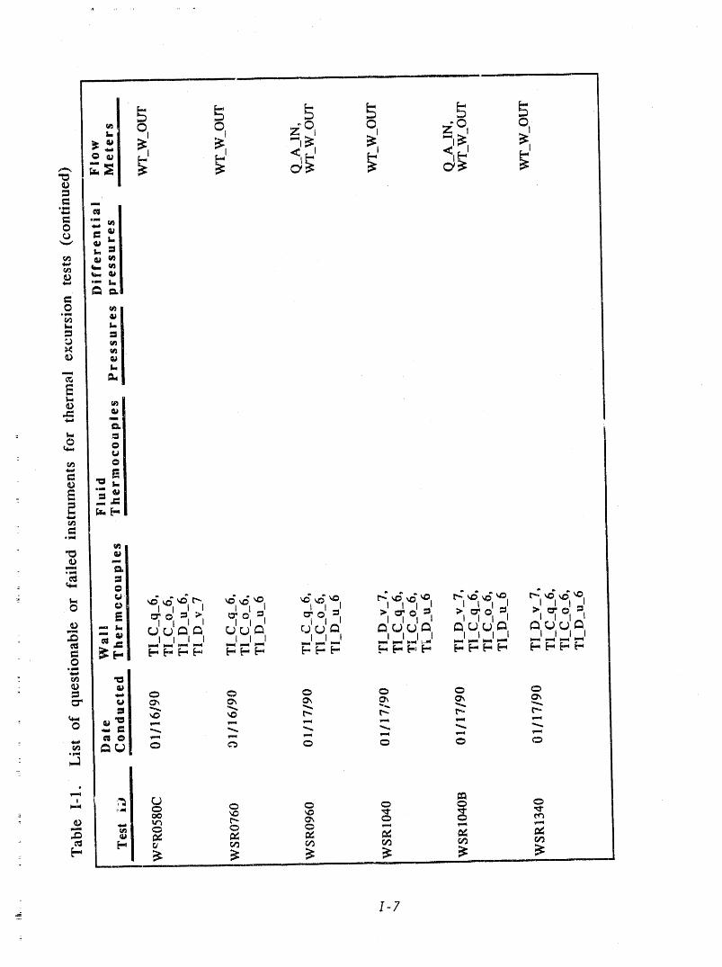
I-7

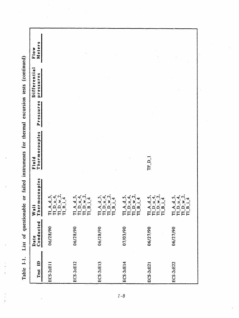
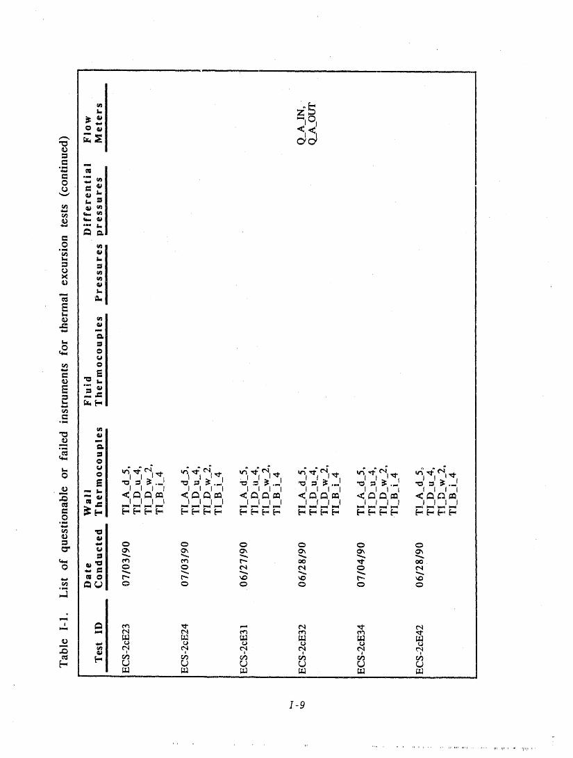
/-9

r

Appendix J

Experimental Data Summary for INEL ThermalExcursion Tests (ECS-2, WSR, and ECS-2cE tests)

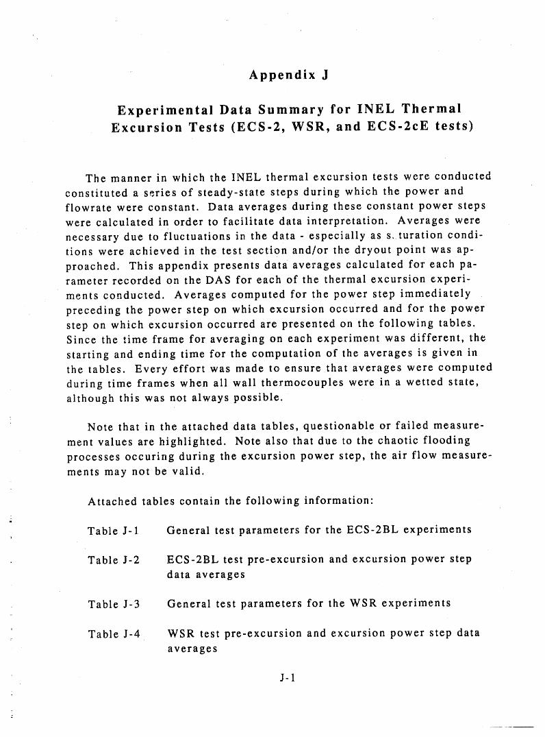
Appendix J

Experimental Data Summary for INEL ThermalExcursion Tests (ECS-2, WSR, and ECS-2cE tests)

The manner in which the INEL thermal excursion tests were conducted

constituted a series of steady-state steps during which the power andflowrate were constant. Data averages during these constant power steps

were calculated in order to facilitate data interpretation. Averages were

necessary due to fluctuations in the data- especially as s turation condi-tions were achieved in the test section and/or the dryout point was ap-

proached. This appendix presents data averages calculated for each pa-rameter recorded on the DAS for each of the thermal excursion experi-

ments conducted, Averages computed for the power step immediately

preceding the power step on which excursion occurred and for the power

step on which excursion occurred are presented on the following tables.Since the time frame for averaging on each experiment was different, the

starting and ending time for the computation of the averages is given inthe tables. Every effort was made to ensure that averages were computed

during time frames when ali wall thermocouples were in a wetted state,

although this was not always possible.

Note that in the attached data tables, questionable or failed measure-

ment values are highlighted. Note also that due to the chaotic flooding

processes occuring during the excursion power step, the air flow measure-

ments may not be valid.

Attached tables contain tile following information"

Table J-1 General test parameters for the ECS-2BL experiments

Table J-2 ECS-2BL test pre-excursion and excursion power step

data averages

Table J-3 General test parameters for the WSR experiments

Table J-4 WSR test pre-excursion and excursion power step data

averages

J-1

Table J-5 General test parameters for the ECS-2cE experiments

Table J-6 ECS-2cE tests pre-excursion and excursion power step

data averages.

i

J-2

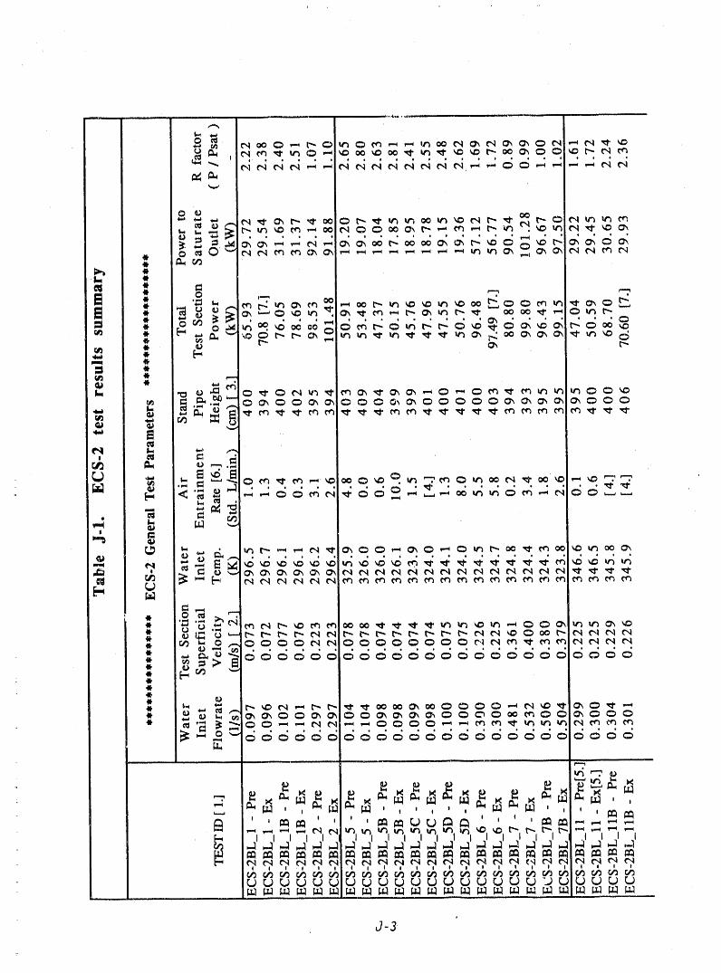
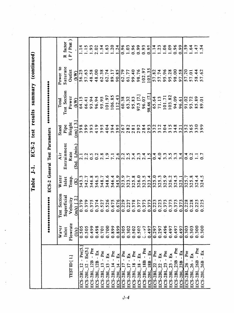
J-4

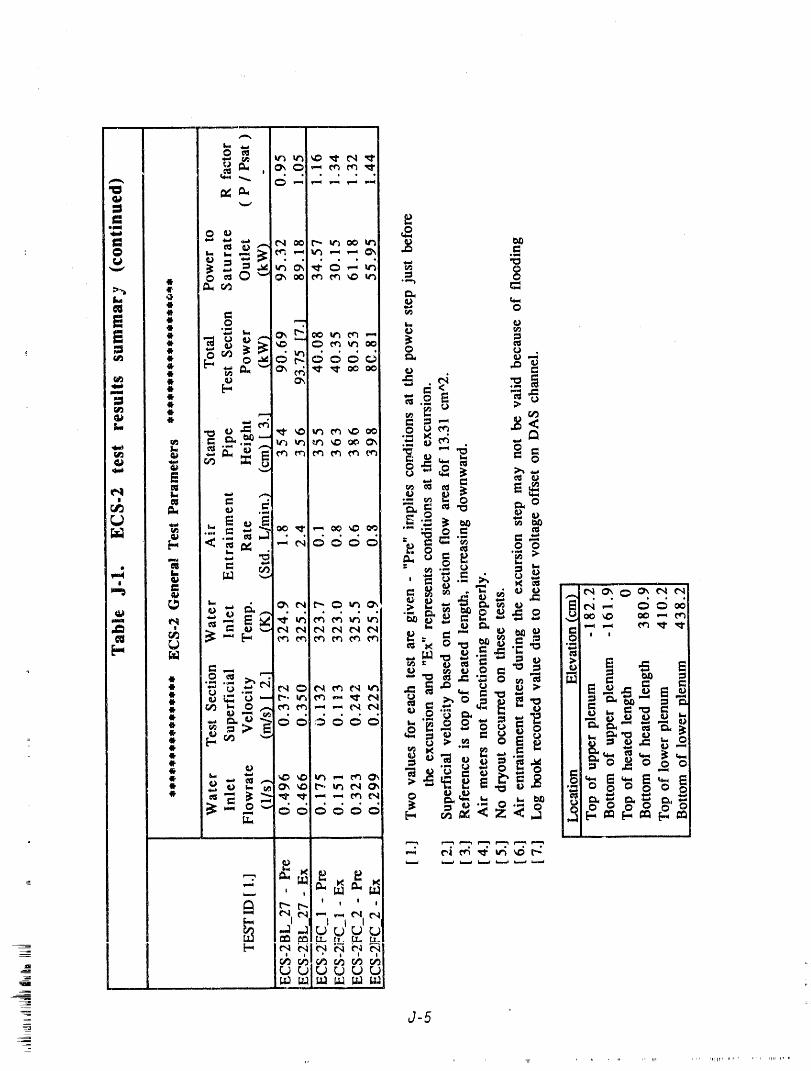
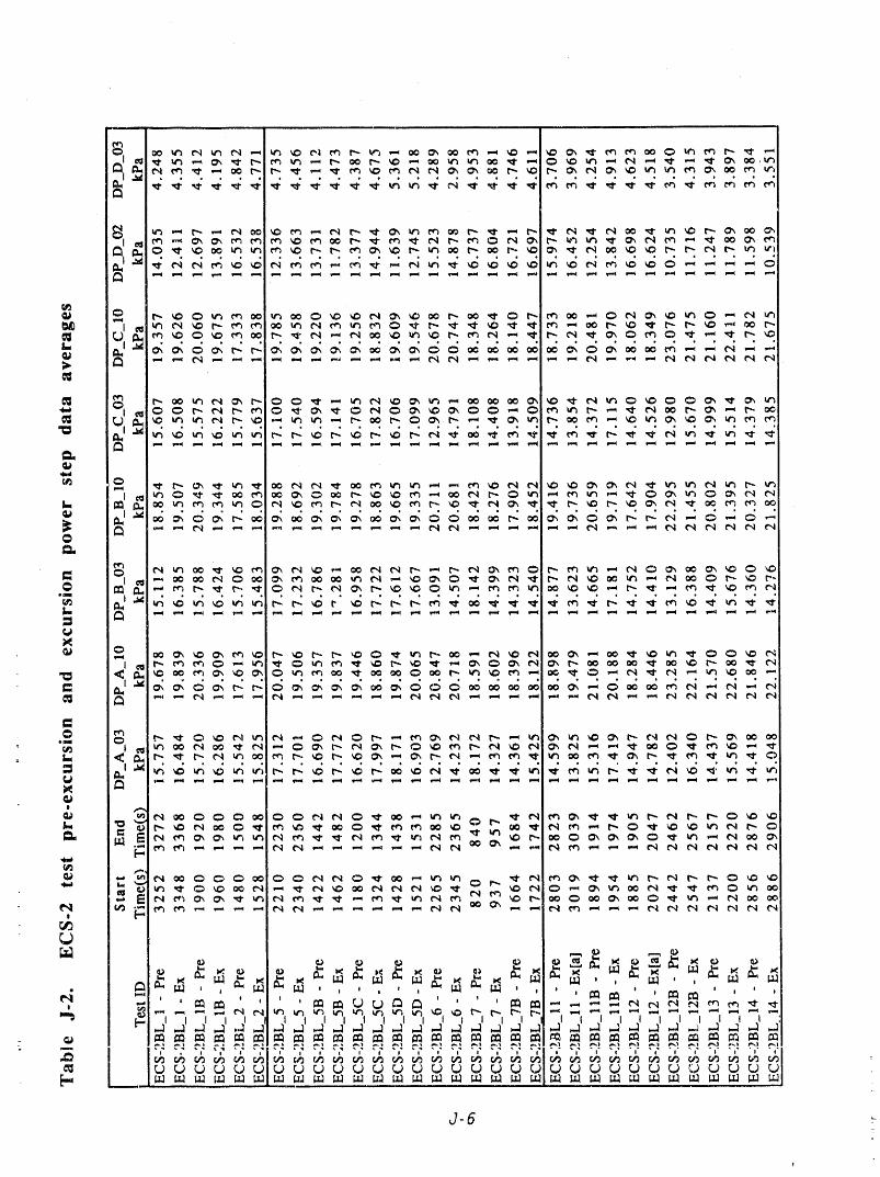
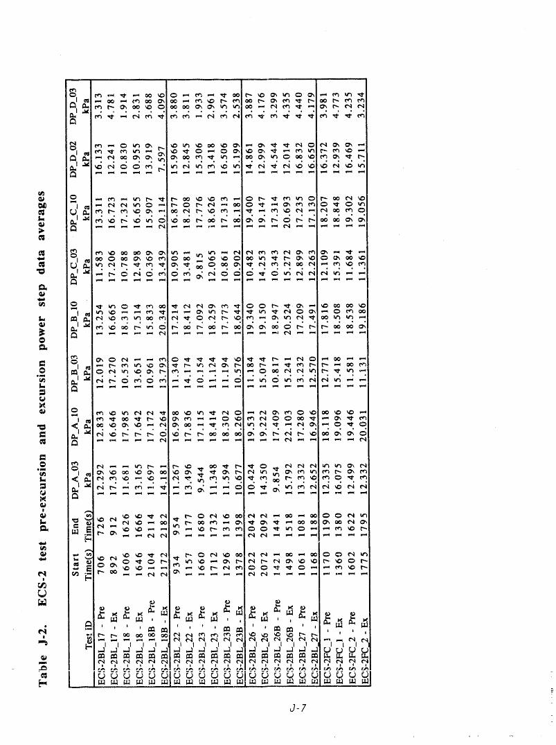
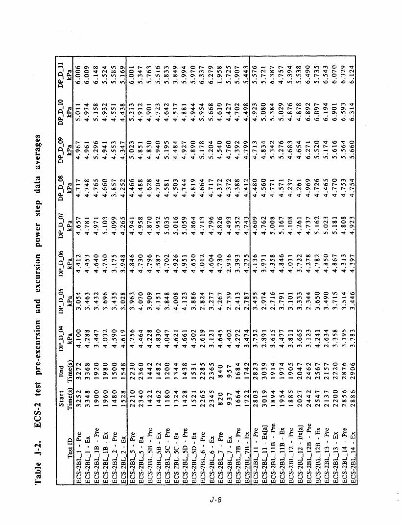
,-, _ _ _ ,.- _ _r_ ,_1- (_1 _,, _'_ r-- _ _'_ _ _ _ _:) _:> ,_- t--. '_t" _ O _ _ _ _ _ _ _ _ __,

c_

@ .I,_

I= - _-,_ md _nd M_m,_d,_ _ mM m,_ _Mdm_ _ mdd_,_mmmd

@ ---

. N

_ ,

I I I I I I I I I I I I o I, ' ' _ _ ' I=

_jl _11 ..I _jI I _._1 I ..)1 .jI I _.jI .._1 .i _jI _.jl _jI _jI

r..J r,j r..j [.j r.j r.j r..j L) L) [J CJ r..J r,.j r..J rj r.j rj L) r..j r,j r.j r.j r.J r,j r,.J L) F.J rJ L,)

J-8

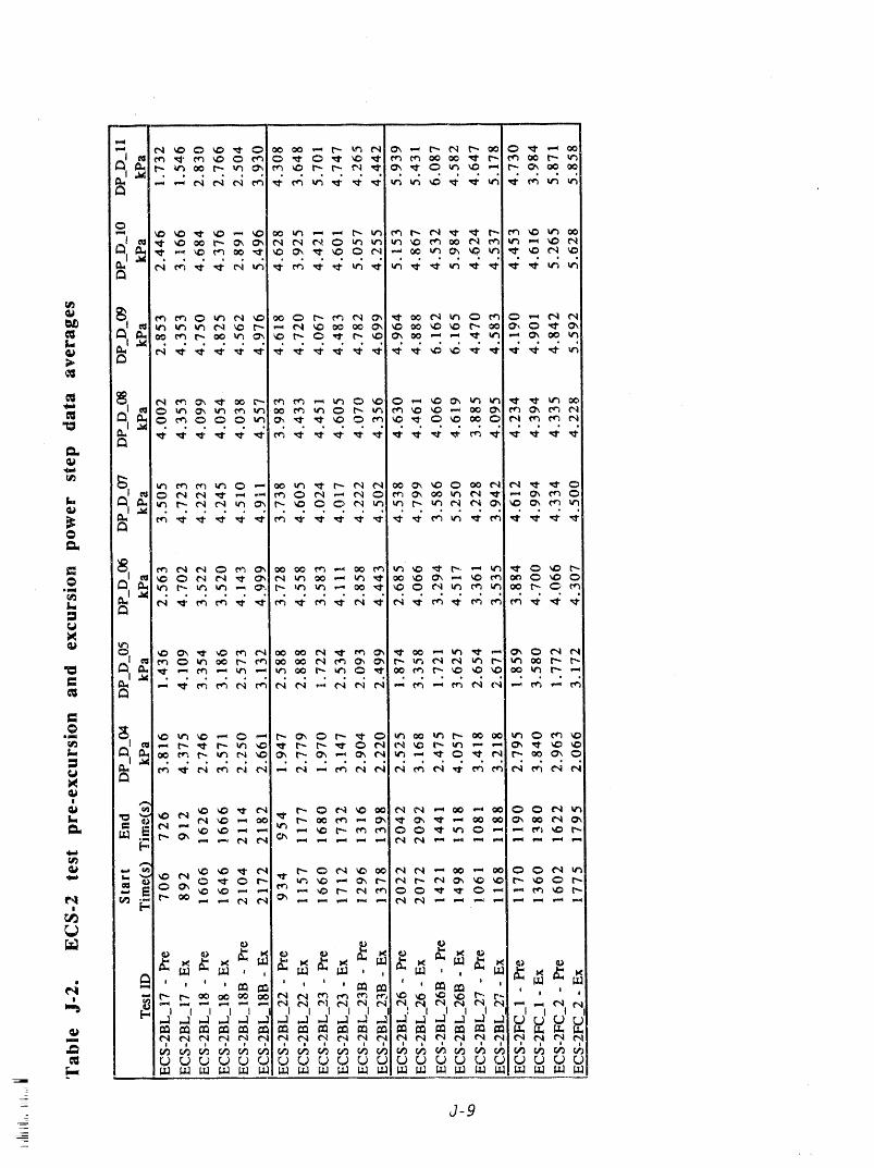
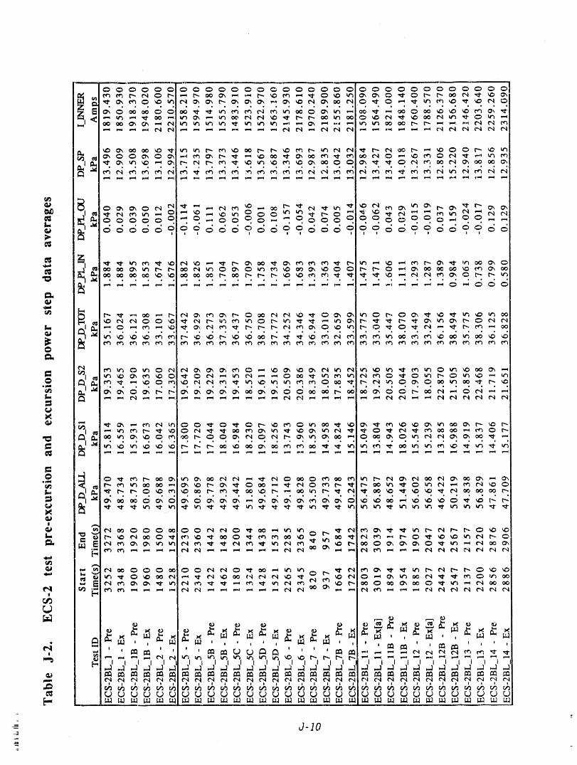
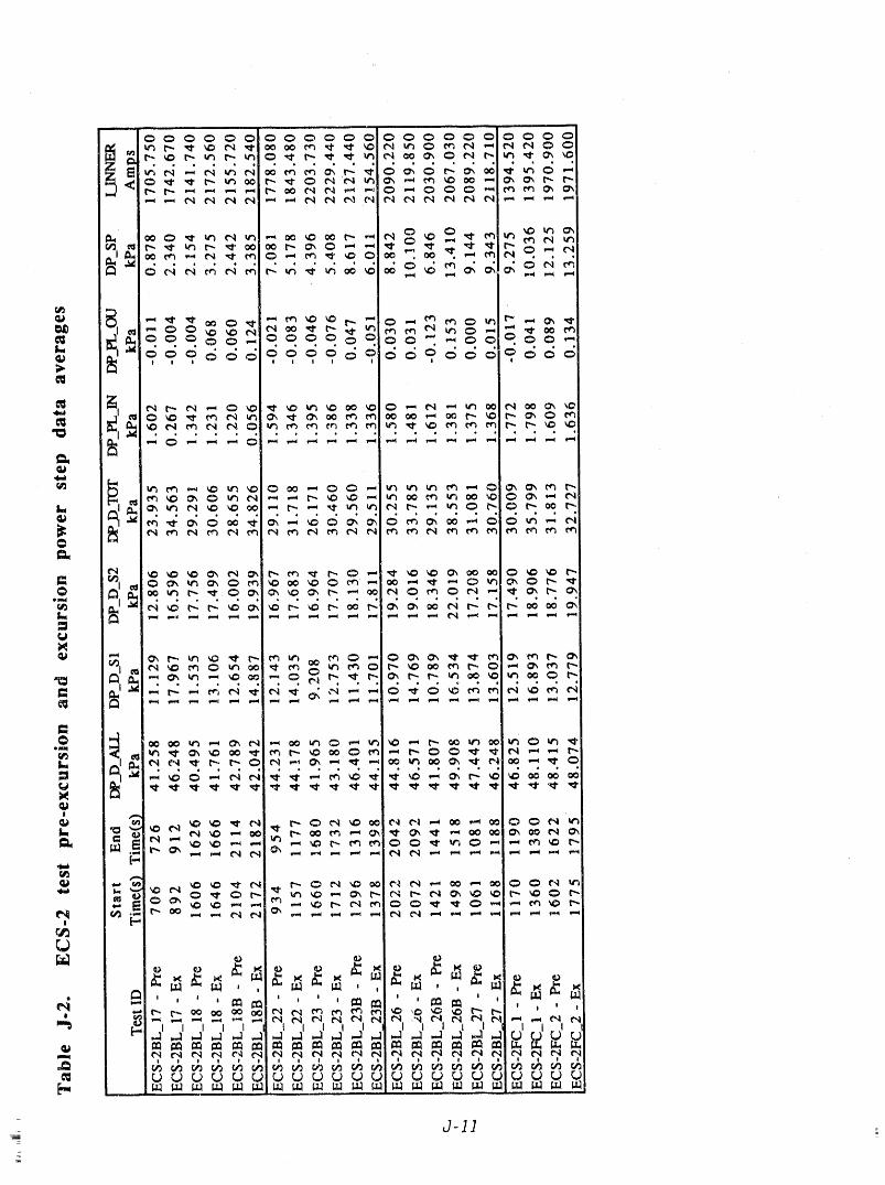
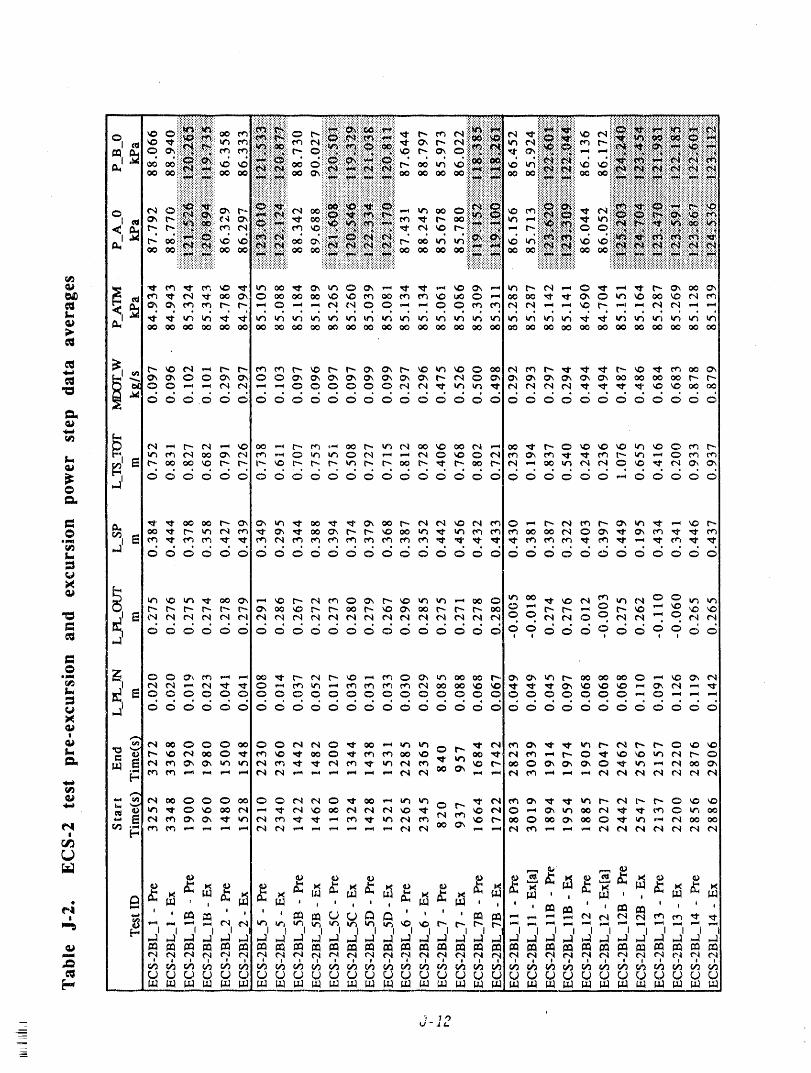
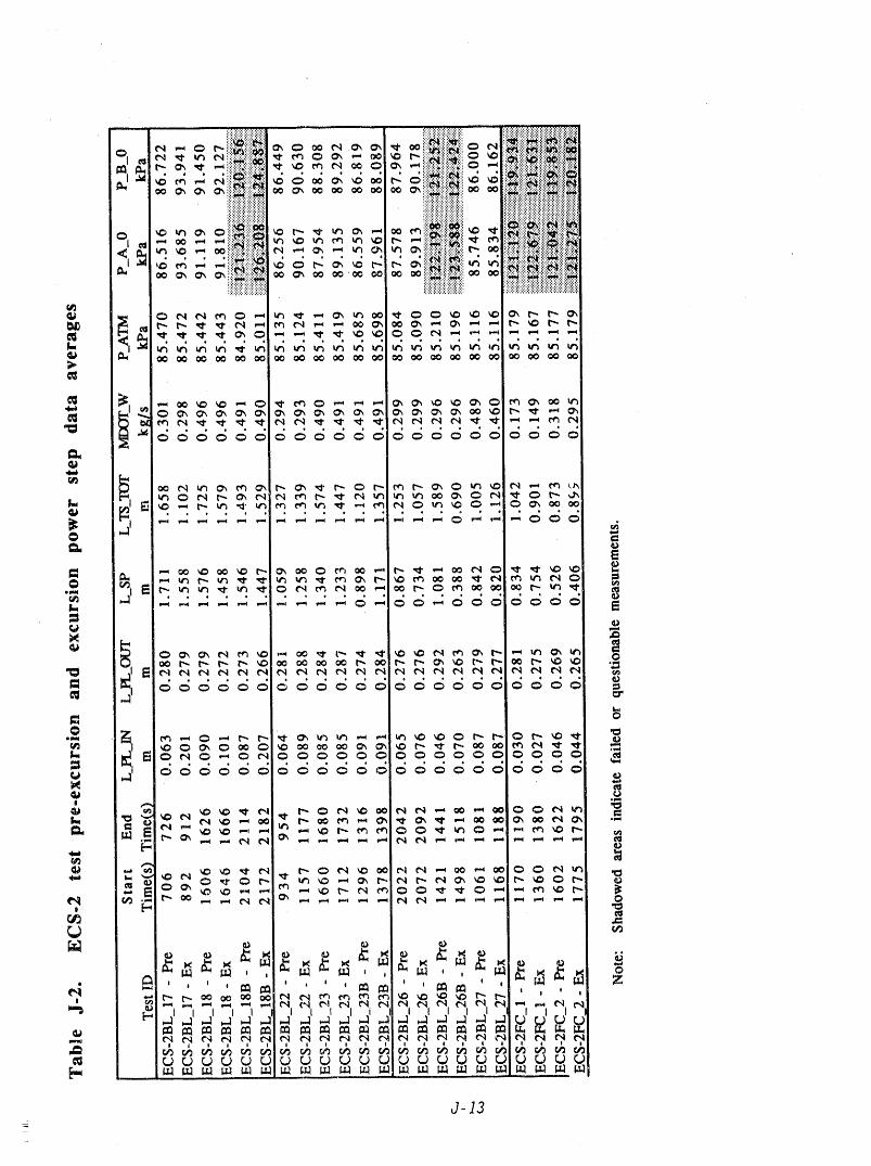
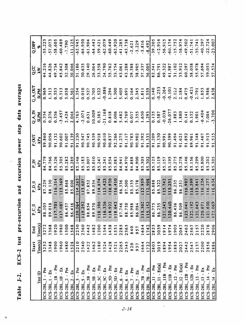
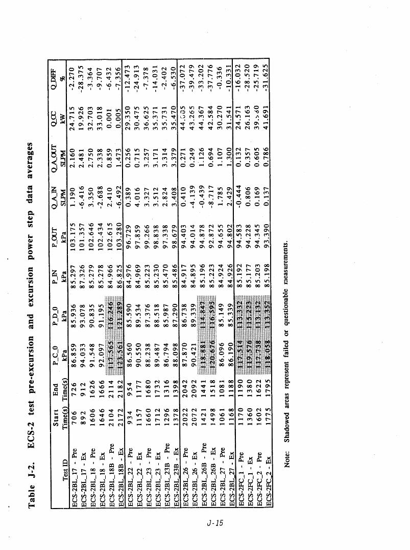
J j ! ! I ! I ! !

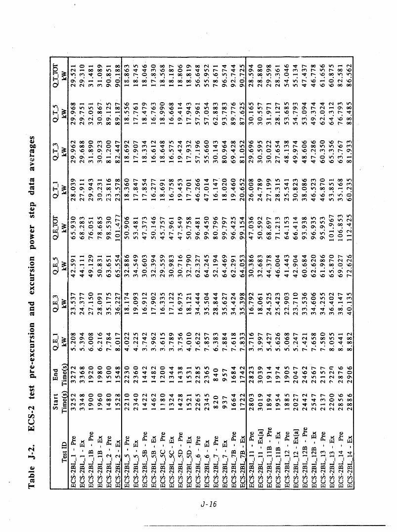
v

J-16

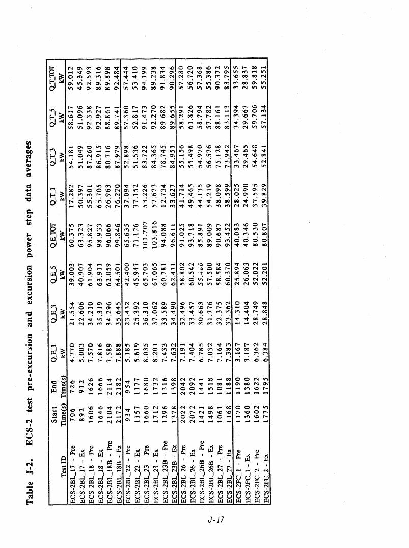
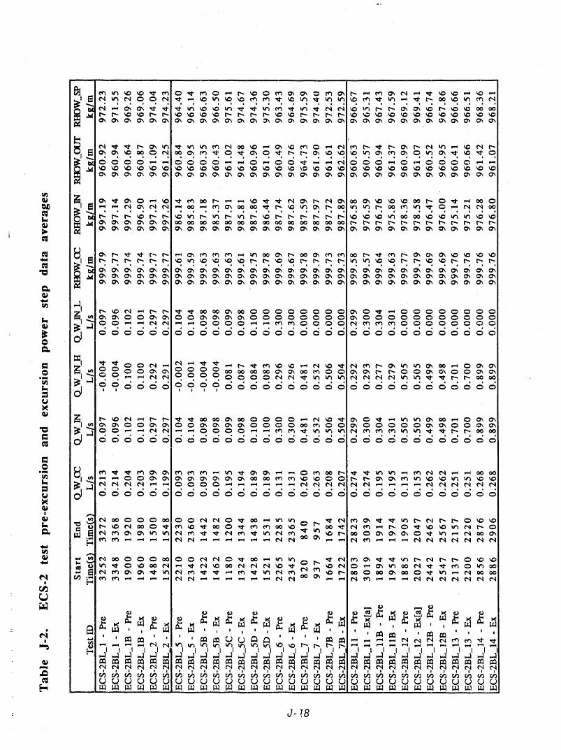
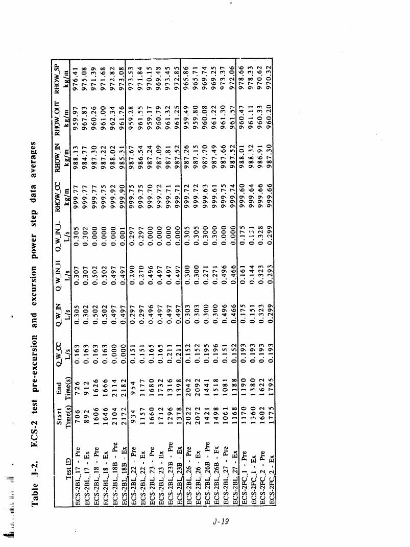
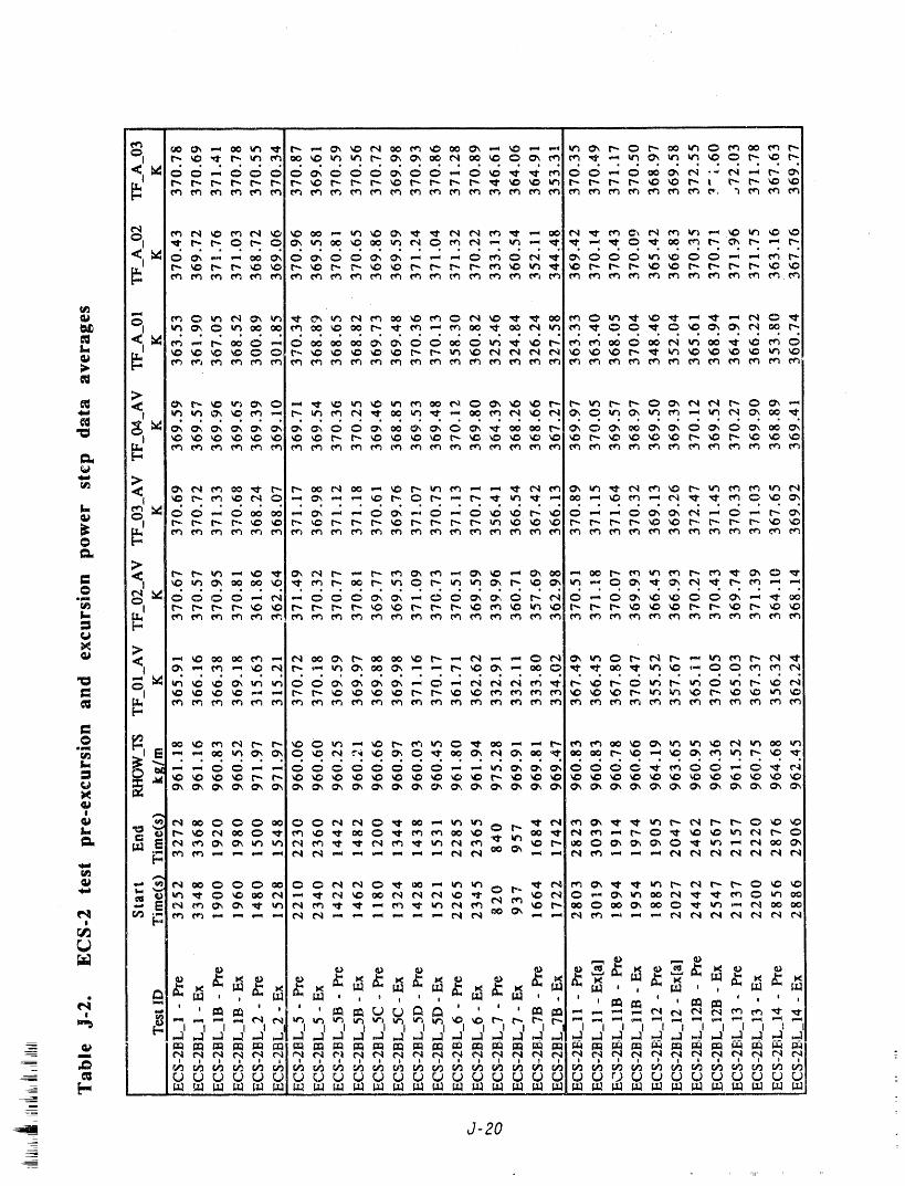
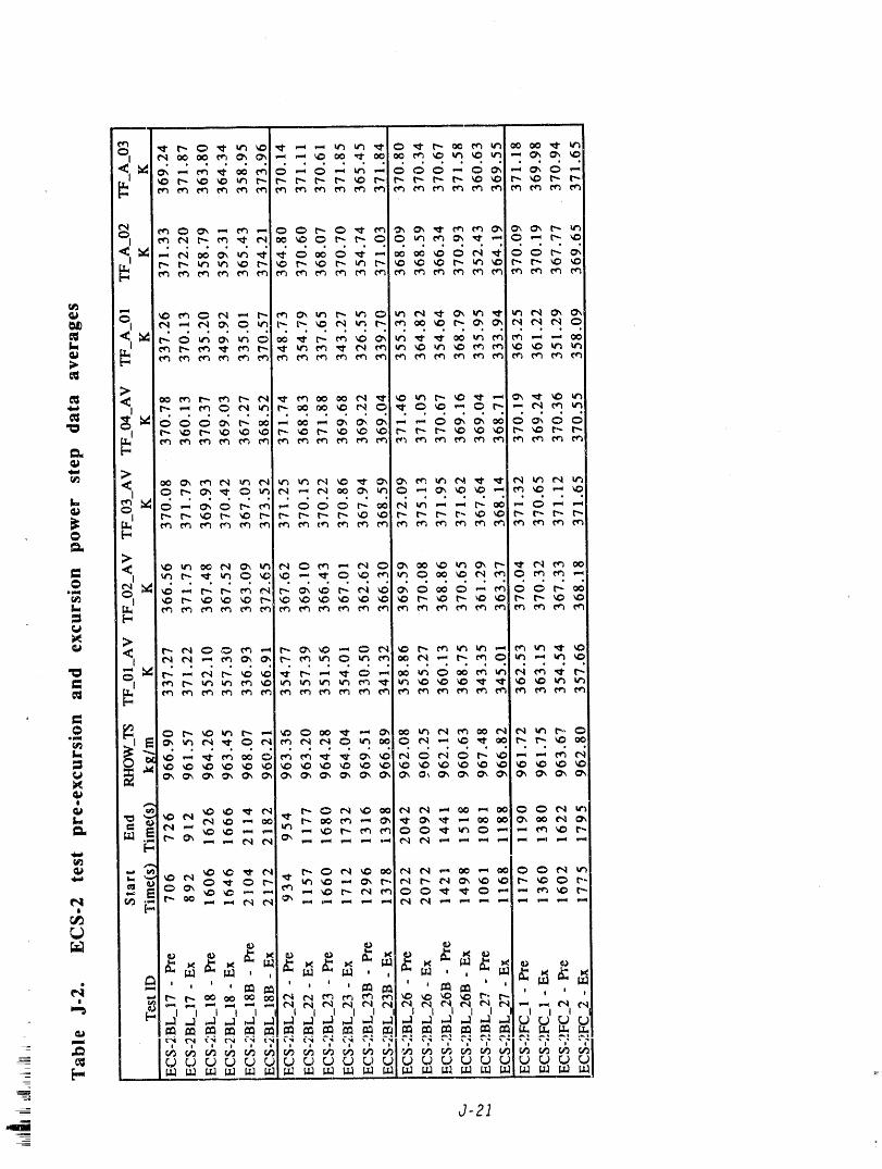
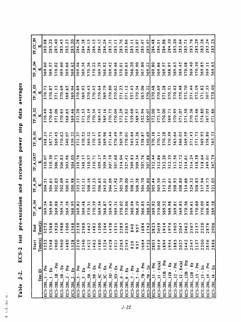
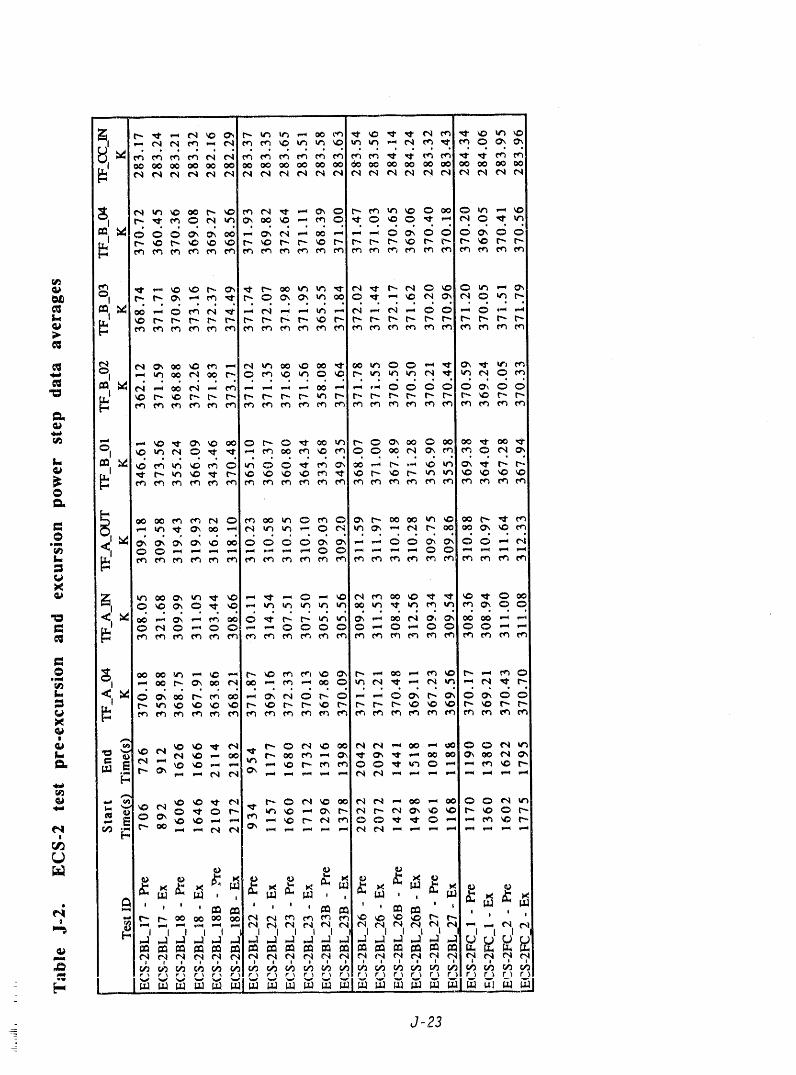
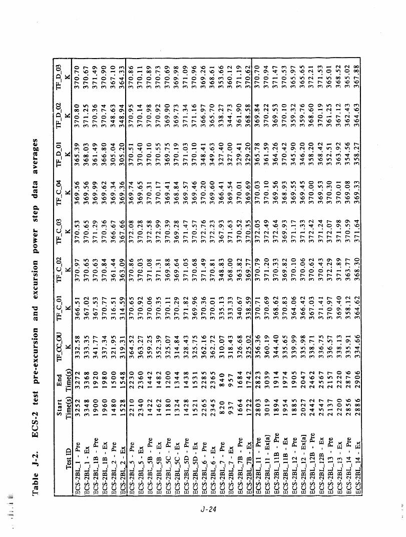
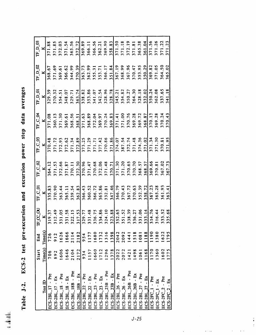
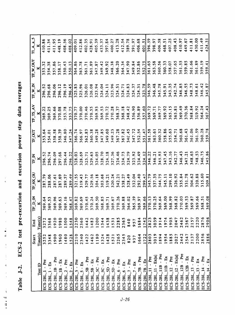
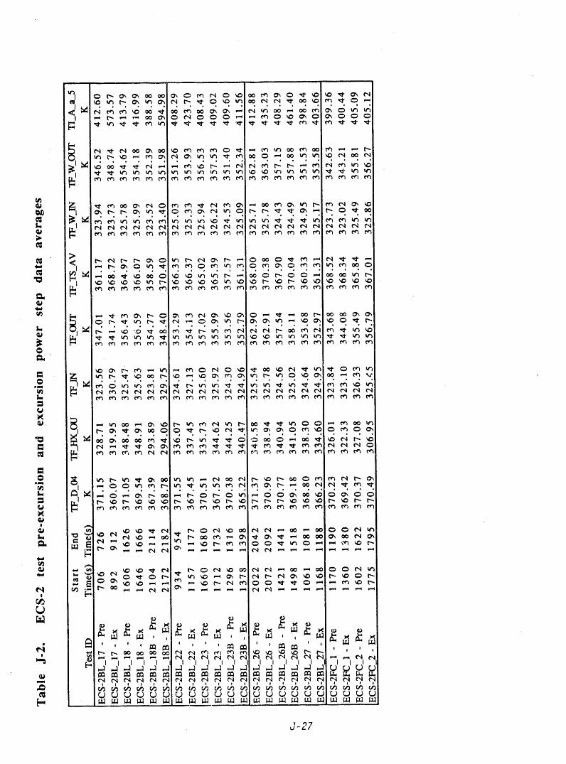
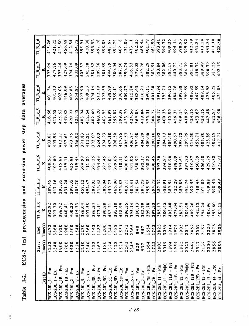
J-28

_

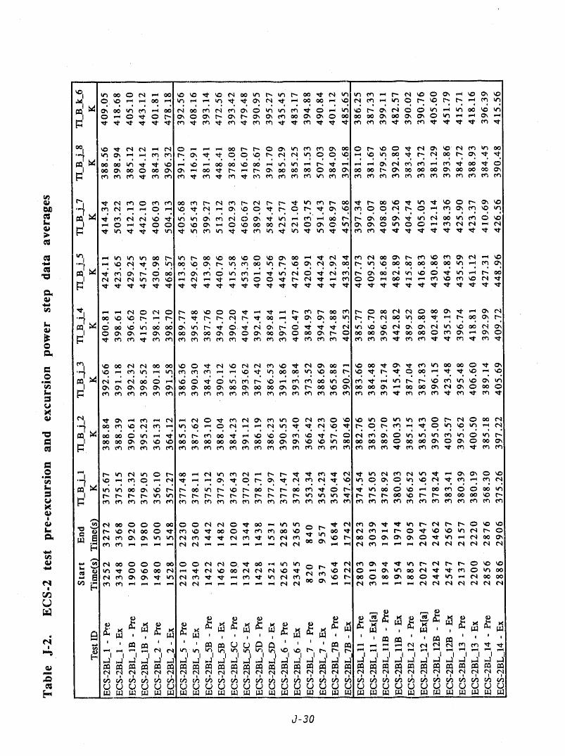
J-30

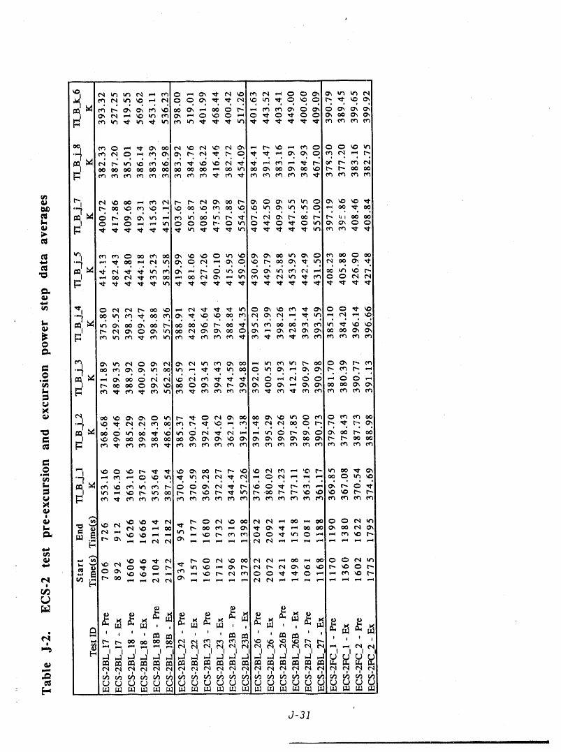
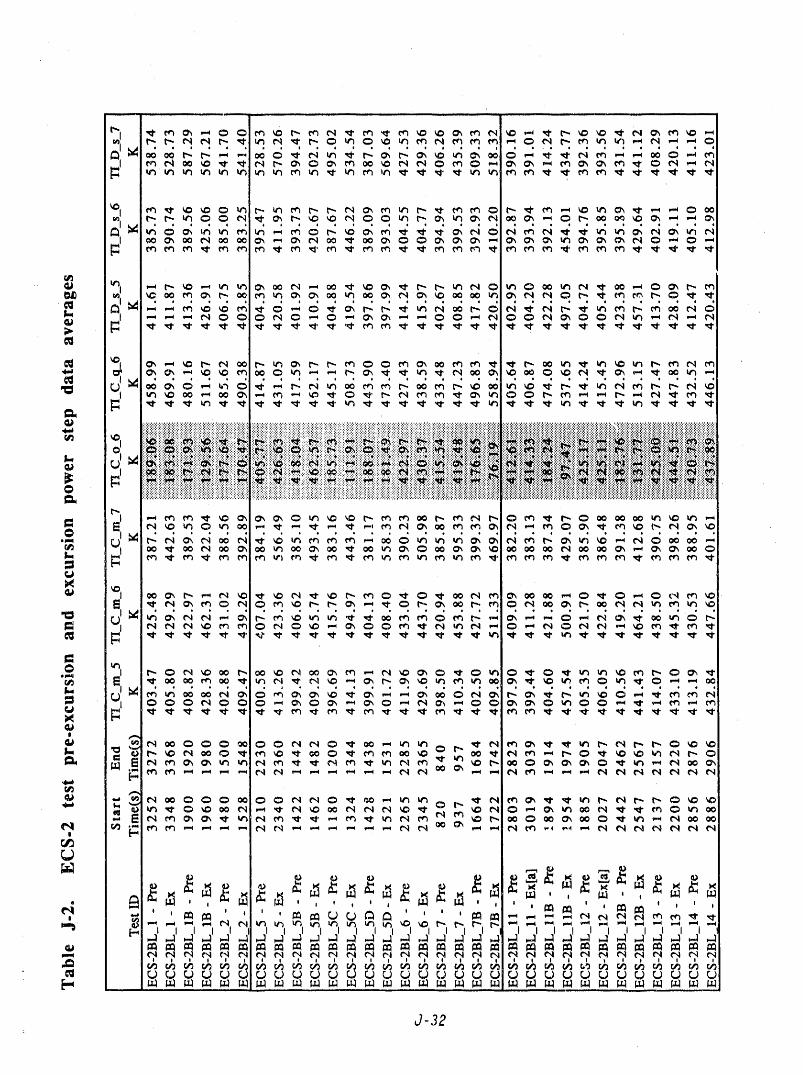
J-32

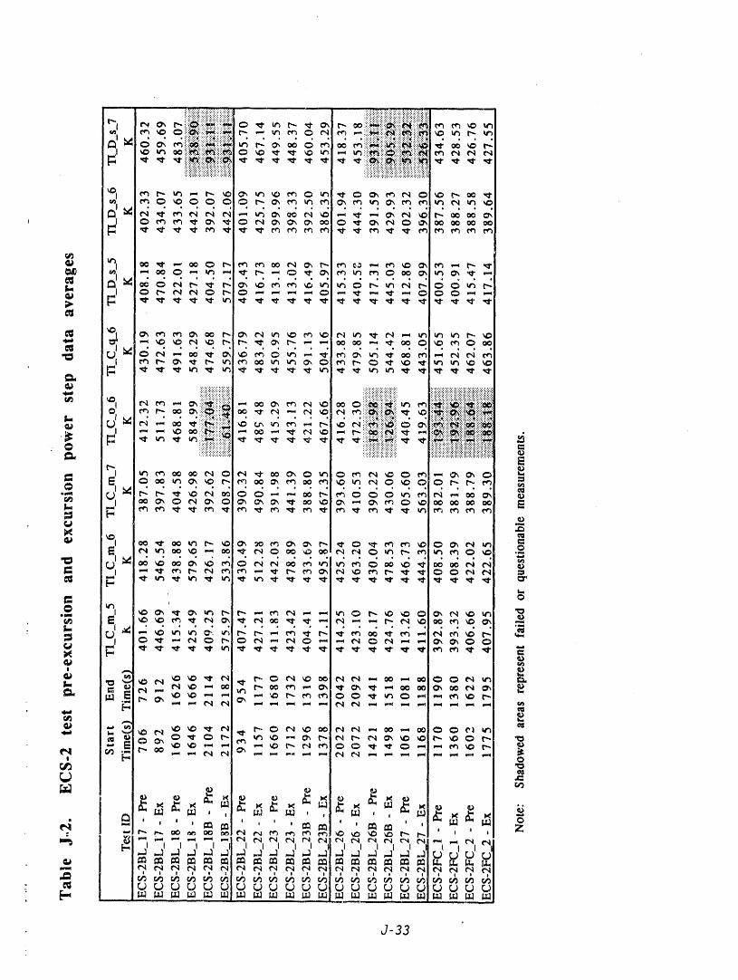
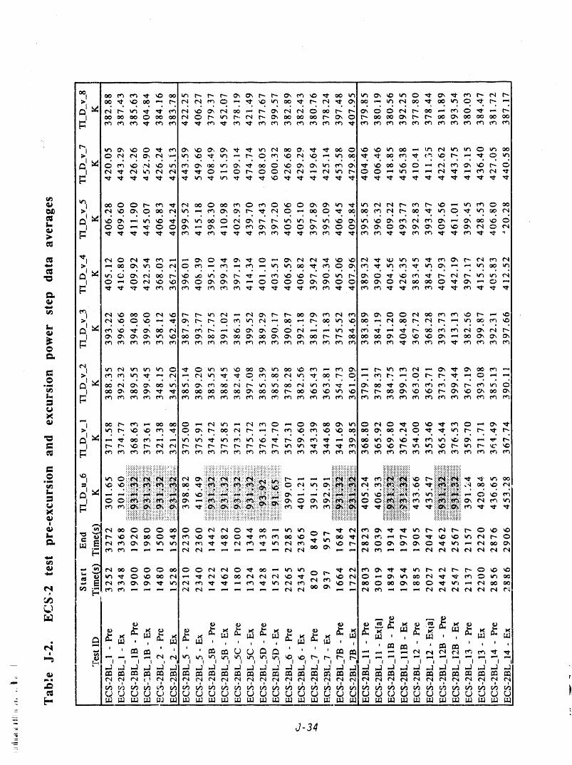
00.

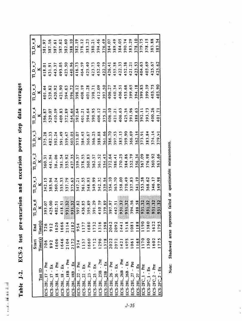
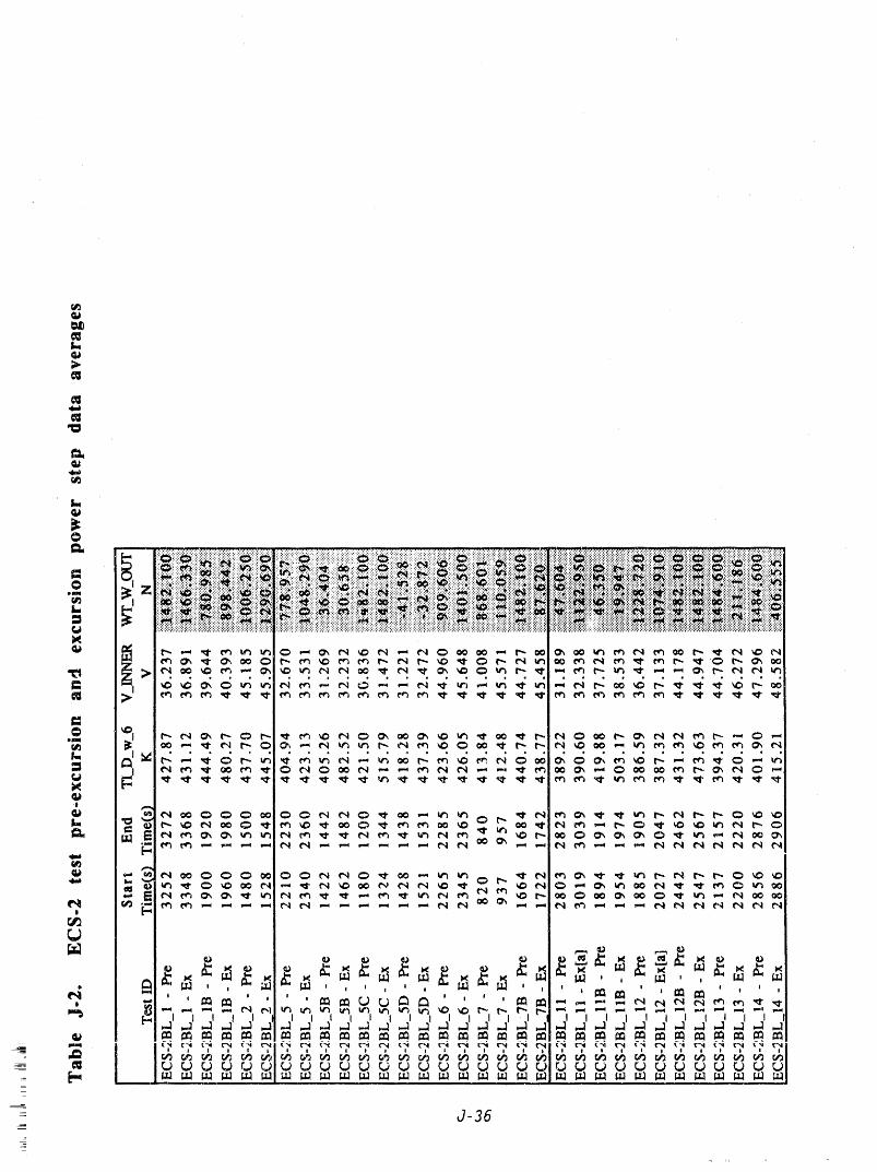
r,_(Pmm

0

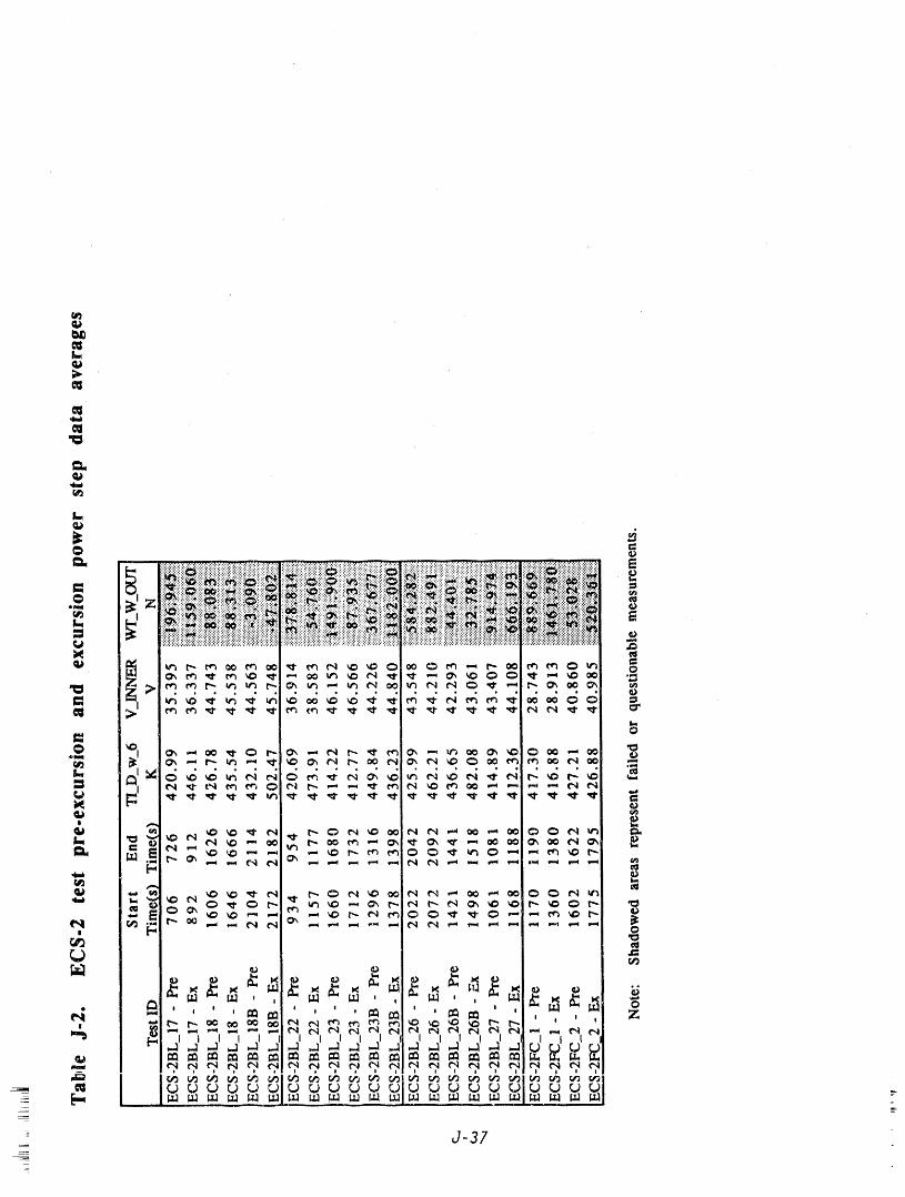
Qa

mlf.

c_

0.,ii

I.Qa

= _ i i!ii!i!iiiiii_iii::iiiiiii!iiiiiiiii::i::i::i!iiiii::iiiii::iii::i::!::...............................:............. ::_:_:_i_i::::::_::_i_i_i::iiii::ii::ii::::_:::_=

m

=!__, , , , ,

.5 _..I("II,_ll_jl .jl I }I _jl _jl I

__ _ _, _, _ _,_,_,

J-37___--.=_

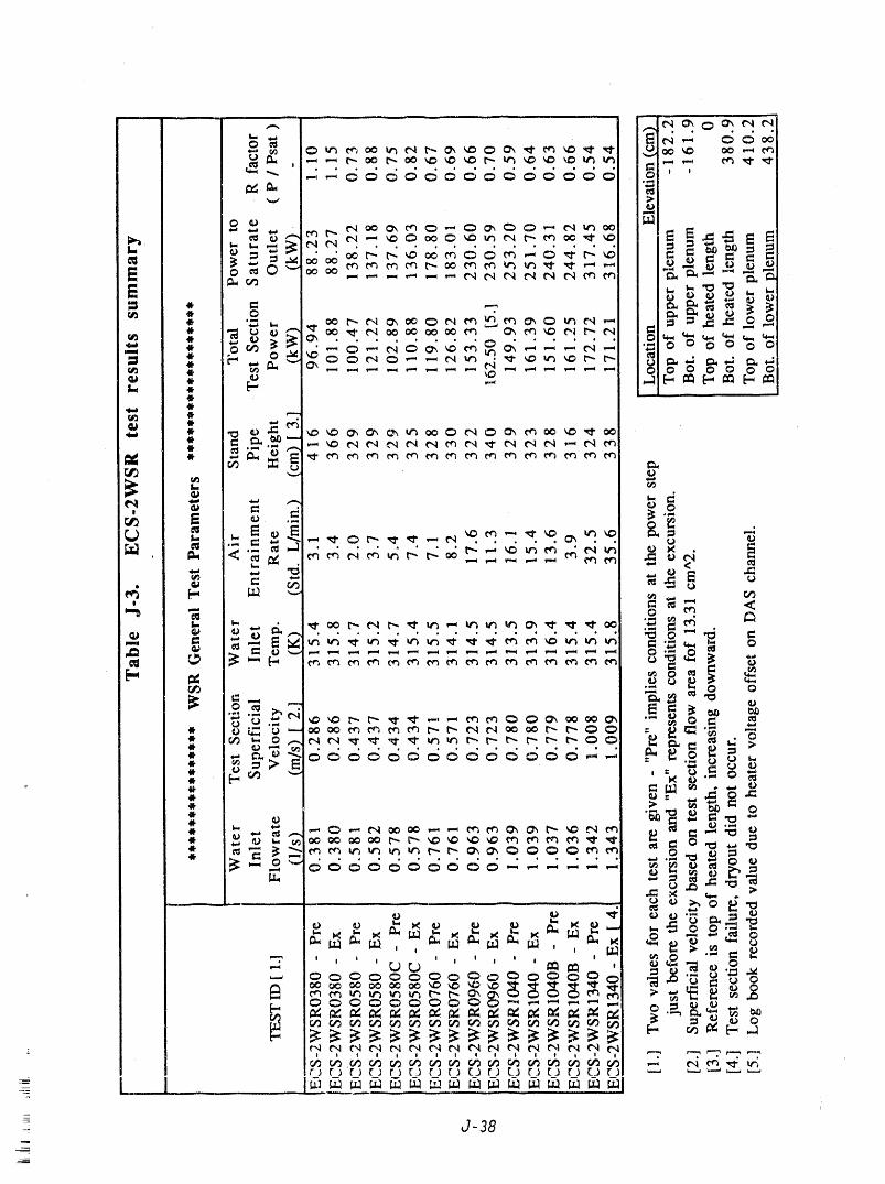
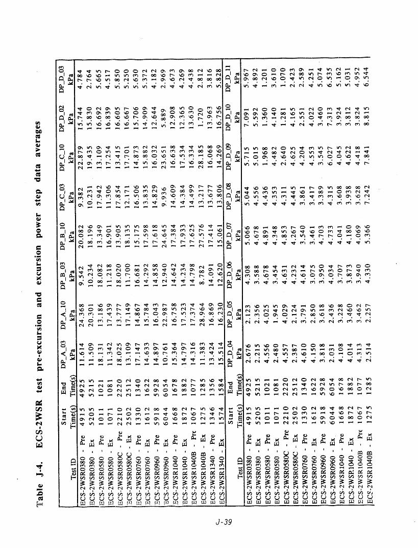
J-39

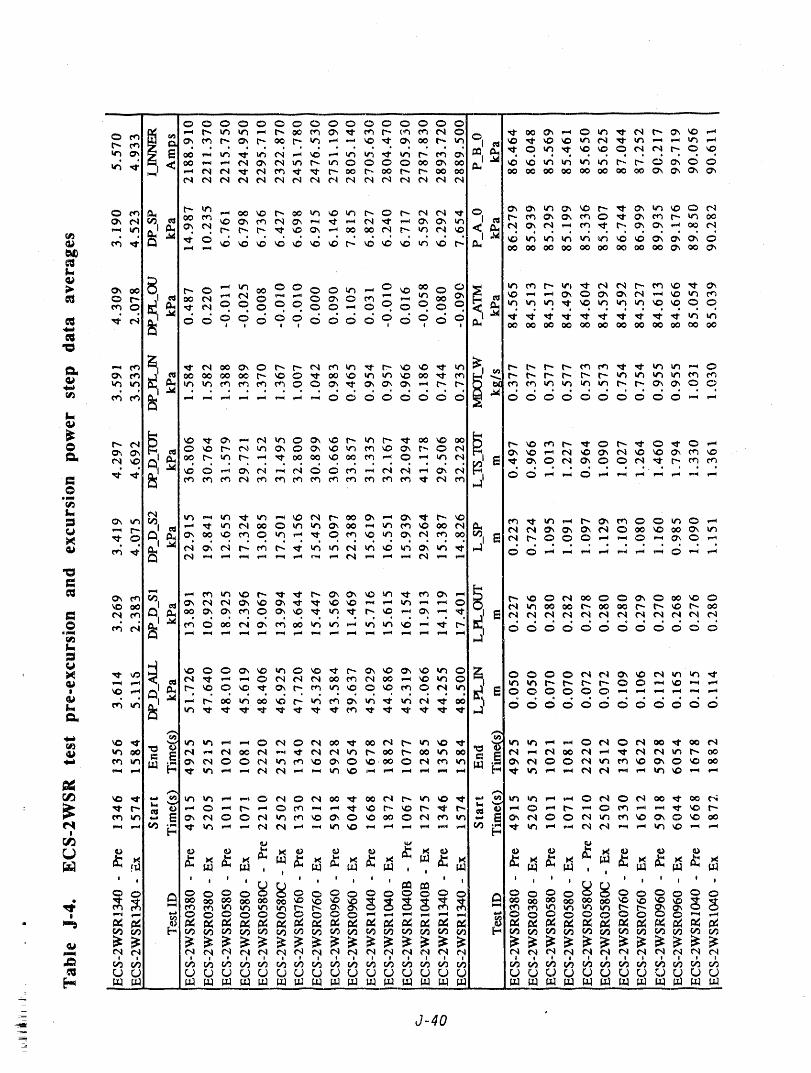
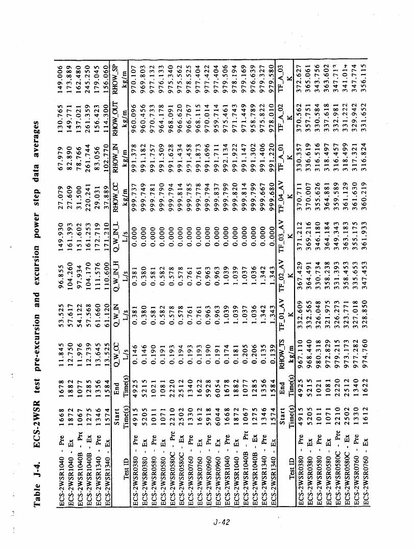
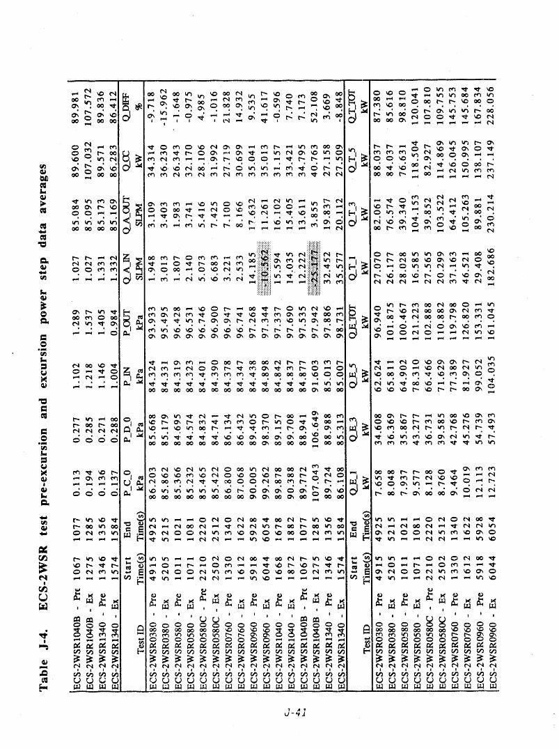
% I

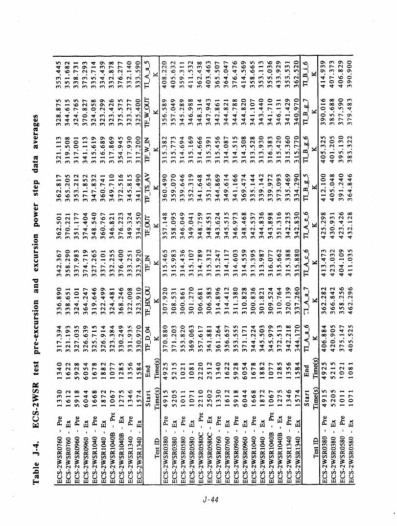
J-44

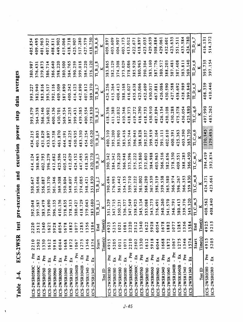
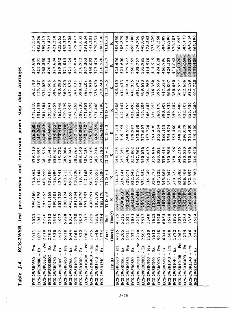
J-46

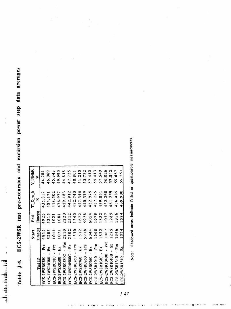
l.Qa

0._a

00.

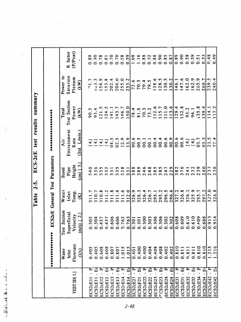
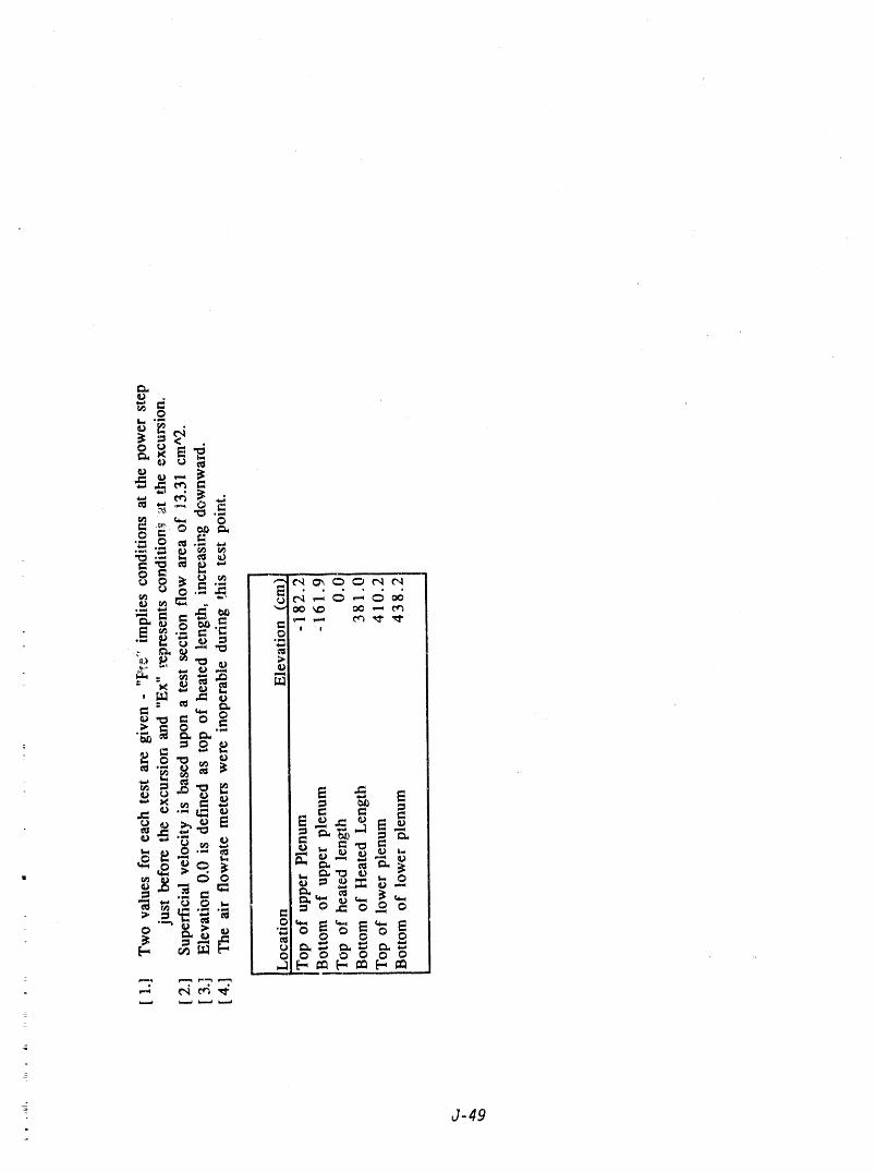
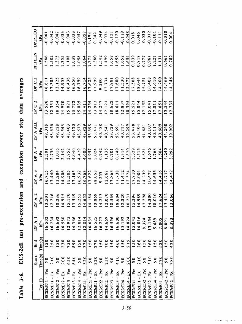
_,, ,... ,l

' 6666666666666666666666o, 61I ! I ! ! I ! I I I, I I I I ! I ! I

I_. _ (_1 u"_ _'_ oo _o oo ,_" _ _D _ _ oo _ c_l ,_t" _ Qo _- ,'_ _ _ _ _41

................ 6666 ' 661

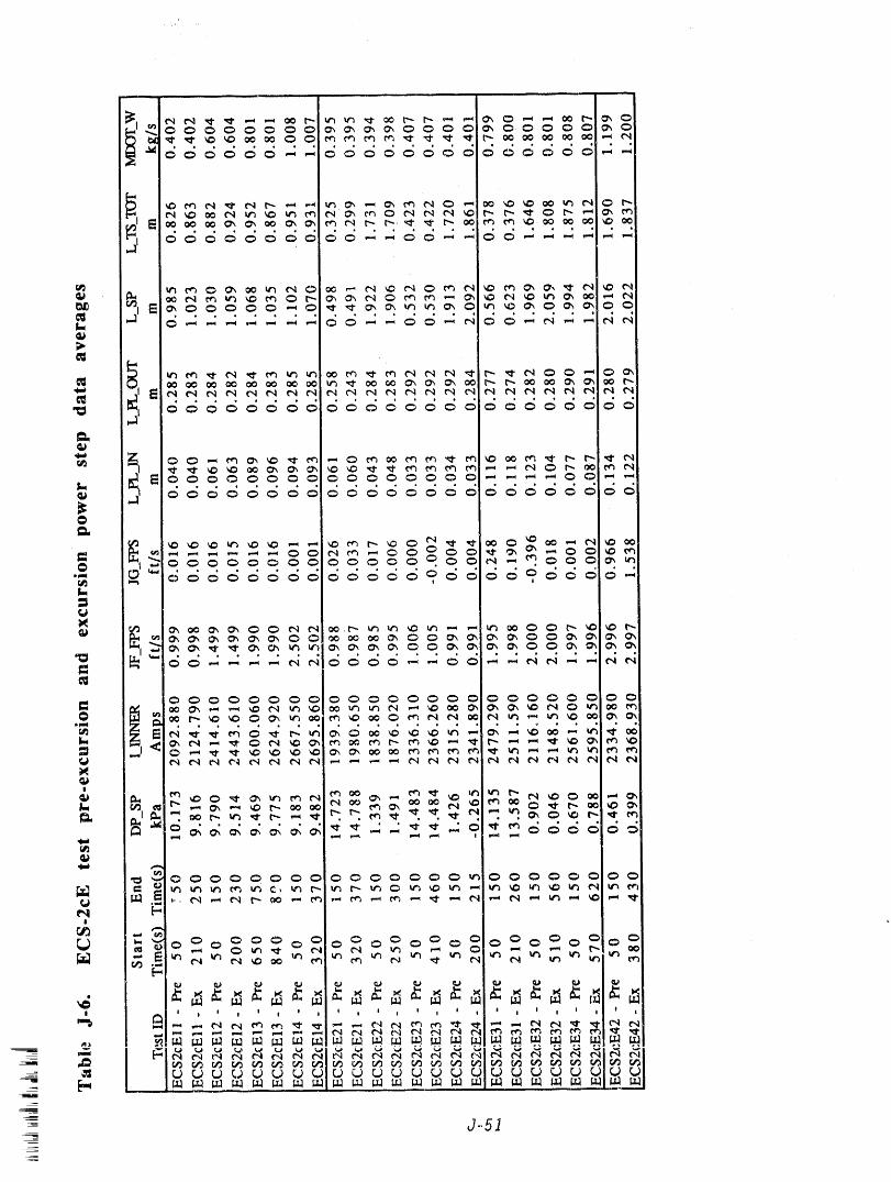
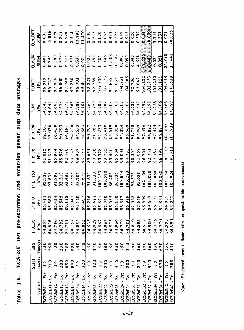
: J-52

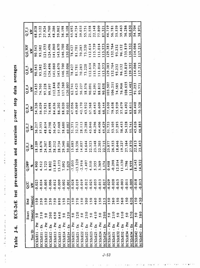
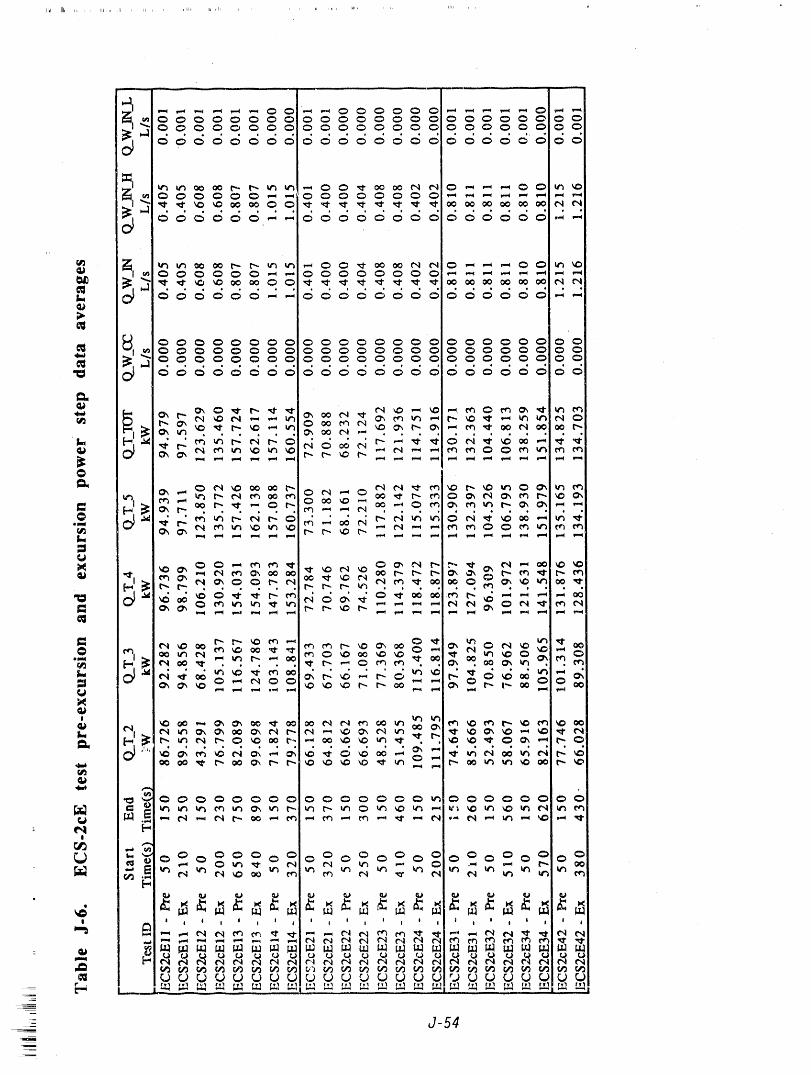
J_ I_ .... JL .... H ,

,1,, __.

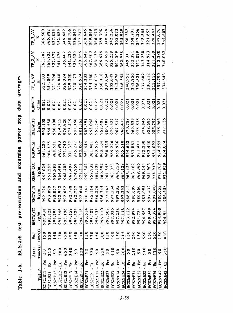
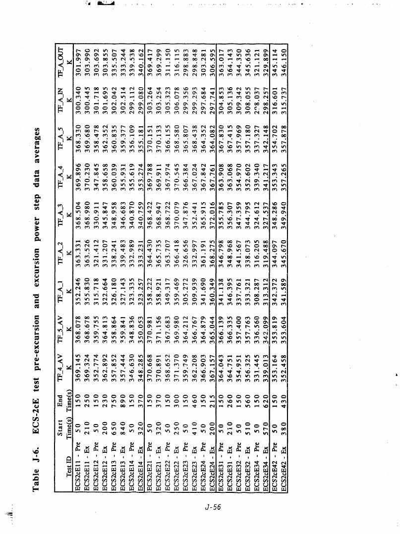
:ilii_

- J-56

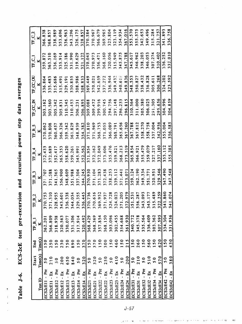
J-57

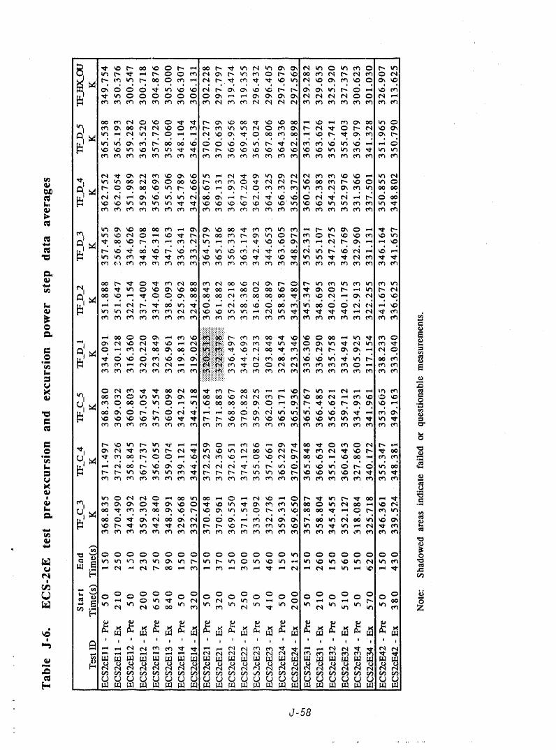
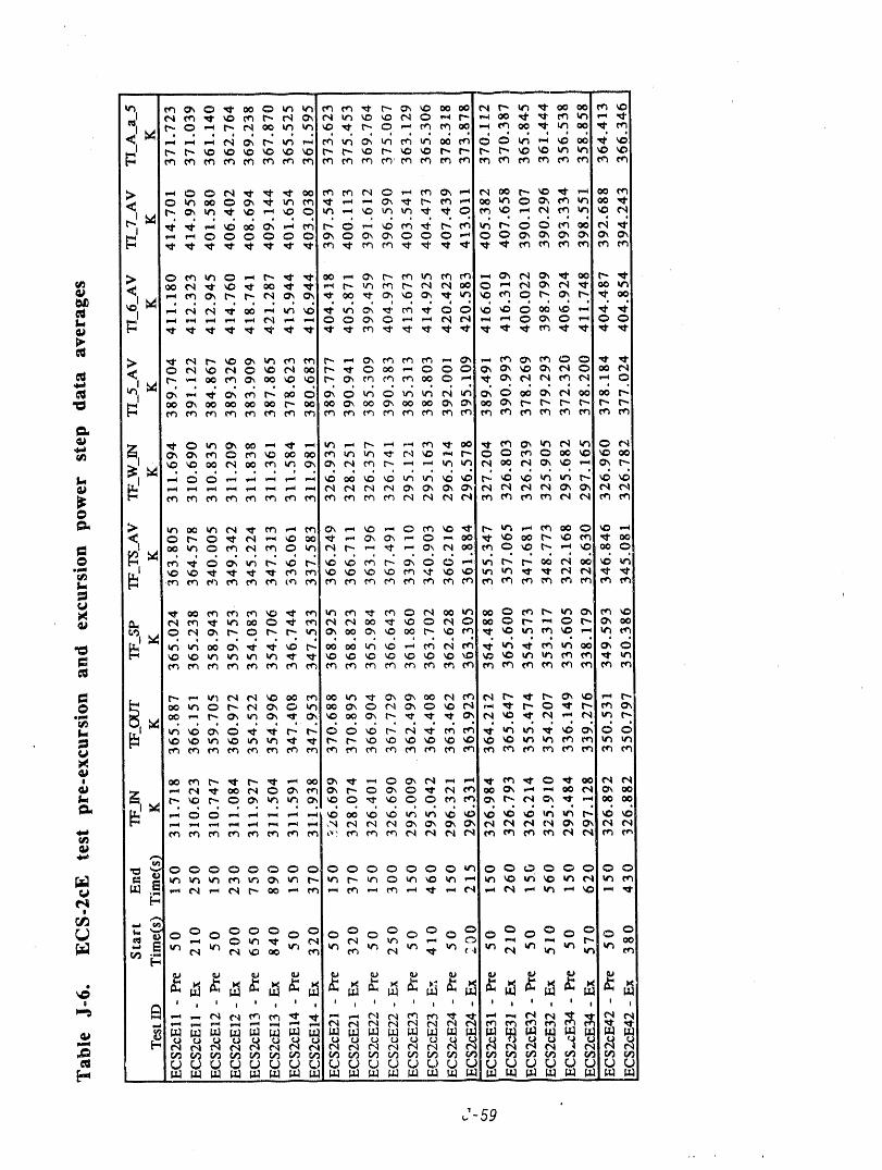
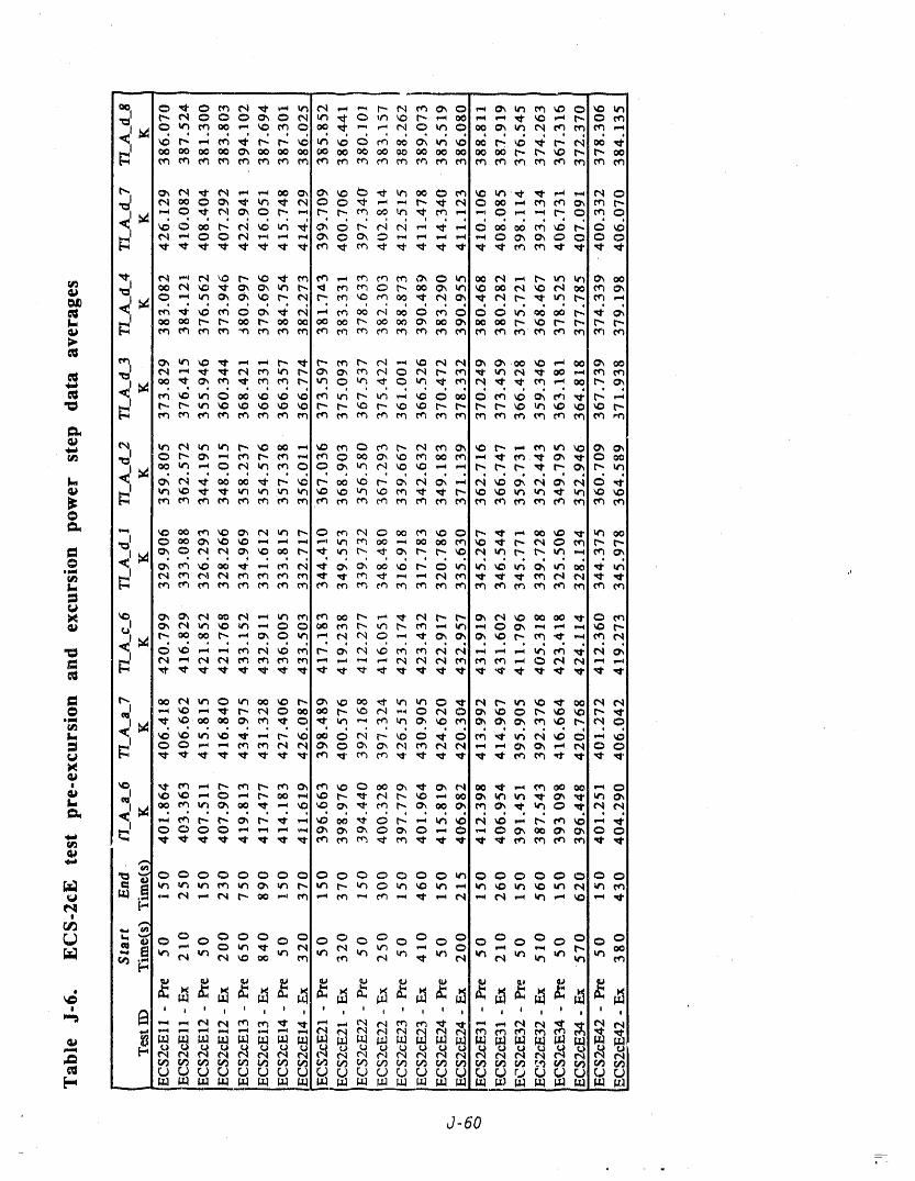
J-60

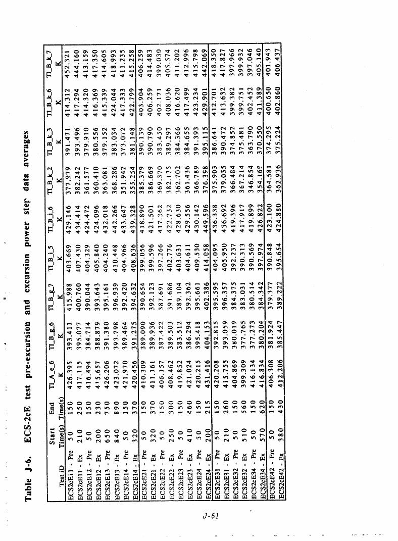
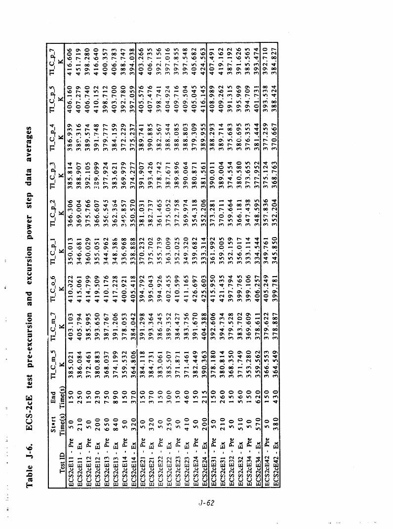
J-62

,,,, , _ ,,

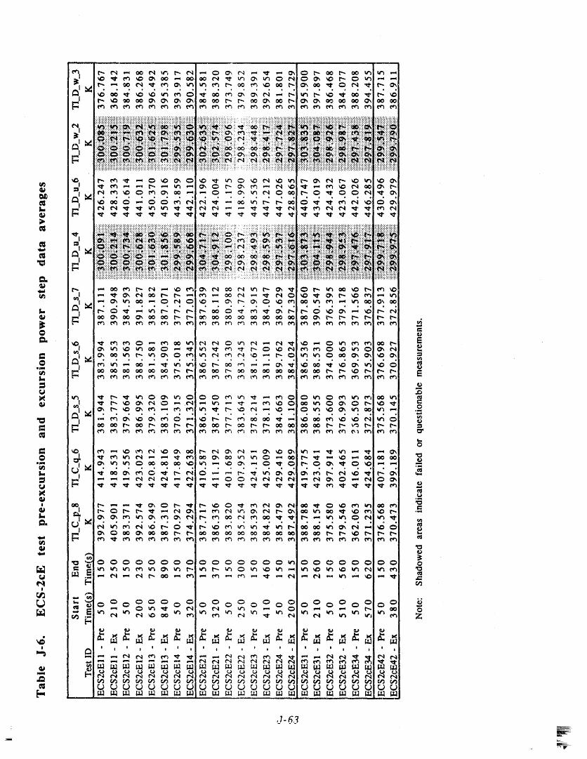
_1 _0 _1" {'_ _,0 _ (_ ,.-_ _ (_1 'Rr _,'_ _ u'_ (_ C:_ _ _,0 r..- _ _ ,.-_ ,.-_

.,,J _ :::::::::::::::::::::::::::::::::::::::::::::::::::::::::::::::::::::::::::::::::::::::::::::::::::::::::::::::::, :::::::::::::::::::::::::::::::::::::::::::::::::::::::::::::::::::::::::::::::::::_,,.-

_1_I t"-. e_ ,_1" _,,.,,_C:) _,a_ 0,_ C:_I_O ,,_- _", _:_ ,,,_ t',,I _l_p _"1 i'--. 0',_ L",,I b _ _ _ _

_1 _ ::::::::::::::::::::::::::::::,.:::::::,:_::::::,::::::::,::;:::::::,.:::::::::,i:;::.*:::::::::*:::::;:::*::::-:; :::;_:::::::::::*;:: :::*:::::::*! ::::*::::::*.::::::;_.::::::*:;::: :_.::::::_

t%I ,"_ 0_ r_ r'- C'4 ,-'_ _ r_ C_ ¢_1 00 f",l _'_ t--. (_, ,_1- 0 t'-. _ 00 _ _ _ _

{=

I,

r._it ," ,"_ ,"_ 04 ('4 ('4 ,-" e'._ ,.'_ ,'_ 0 0 _"4 C',,I ("4 ("4 _..,, r,4 _ _ _ _ _ _

_a

_ _ 0 0 0 0 0 0 0 o 0 o o o 0 0 0 _ 0 0 C::>0 _ 0 0 0 o

r_ ,-,r_ i., .,._ o cD o o 0 o o o o o o 0 o o o ,.,

I I I I I i I I t I I

_ N _INNN NN

,,

,1- fi.':l

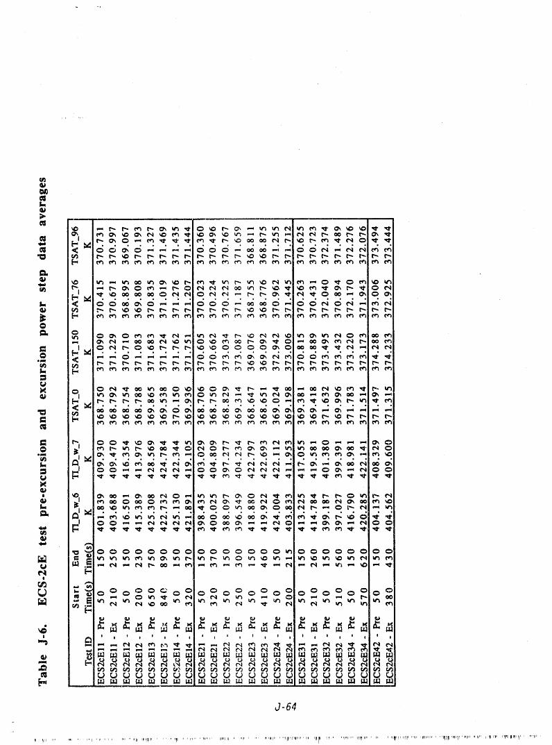
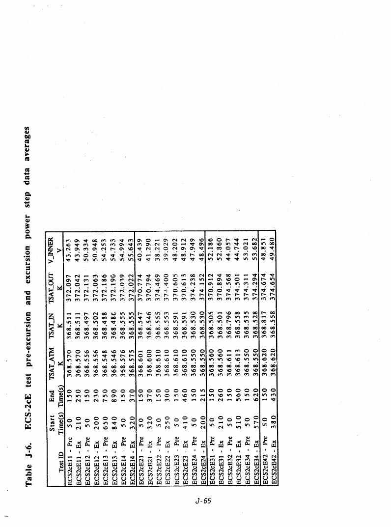
f

i

-i

l ii"̀ .., J i' ..... _............,"'.,'_:".,.-_,._............................,,.,_..:.

i . _ 2____ --

i :-T I I I Irlll I. . I

f

Z

=