THE AMERICAN SOCIETY OF MECHANICAL ENGINEERS345 E 47th St, New York, NM. 10017

The Society shall not be responsible for statements or opinions advanced inpapers or discussion at meetings of the Society or of its Divisions or Sections,or printed in its publications. Discussion is printed only if the paper is pub-lished in an ASME Journal. Papers are available from ASME for 15 monthsafter the meeting.

Printed in U.S.A.

93-GT-25

EFFECTS OF FREE-STREAM TURBULENCE INTENSITYON A BOUNDARY LAYER RECOVERING FROM

CONCAVE CURVATURE EFFECTS

Michael D. Kestoras and Terrence W. SimonDepartment of Mechanical Engineering

University of MinnesotaMinneapolis, Minnesota

ABSTRACT

Experiments are conducted on a flat recovery wall downstream ofsustained concave curvature in the presence of high free-streamturbulence (TI-8%). This flow simulates some of the features of the flowon the latter parts of the pressure surface of a gas turbine airfoil. Thecombined effects of concave curvature and TI, both present in the flowover a turbine airfoil, have so far little been studied. Computation of suchflows with standard turbulence closure models has not been particularlysuccessful. This experiment attempts to characterize the turbulencecharacteristics of this flow. In the present study, a turbulent boundarylayer grows from the leading edge of a concave wall then passes onto adownstream flat wall. Results show that turbulence intensities increaseprofoundly in the outer region of the boundary layer over the recoverywall. Near-wall turbulent eddies appear to lift off the recovery wall and a"stabilized" region forms near the wall. In contrast to a low-free-streamturbulence intensity flow, turbulent eddies penetrate the outer parts of the"stabilized" region where sharp velocity and temperature gradients exist.These eddies can more readily transfer momentum and heat. As a result,skin friction coefficients and Stanton numbers on the recovery wall are20% and 10%, respectively, above their values in the low-free-streamturbulence intensity case. Stanton numbers do not undershoot flat-wallexpectations at the same ReA 2 values as seen in the low-TI case.Remarkably, the velocity distribution in the core of the flow over therecovery wall exhibits a negative gradient normal to the wall under highfree-stream turbulence intensity conditions. This velocity distributionappears to be the result of two effects: 1) cross transport of kinetic energyby boundary work in the upstream curved flow and 2) readjustment ofstatic pressure profiles in response to the removal of concave curvature.

Static pressure

Pd

Dynamic pressure, Pd = 1/2pU2Pr

Molecular Prandtl number.Pref Static pressure at the most upstream pressure tap 2 cm from

the concave surfacePt

Total pressure, Pt = P + Pd

qw Convective heat flux at the wall.

Radius of curvature (negative for a concave surface).Rex Reynolds number based upon distance from the beginning of the

test wall.Ressi Reynolds number based upon displacement thickness.Re82 Reynolds number based on momentum thickness.

St Stanton number, St = Clw/pCp ( Tw — T.)UcwT Local mean temperature.

TI Free-stream turbulence intensity i aru-27Ucw

To. Free-stream temperature.Tw Wall temperature.

T+ Temperature in wall units ((Tw-T)/(Tw-T...))/StMean streamwise velocity.

Uc Local mean velocity obtained by extrapolating the velocitydistribution in the core of the flow.

Root-mean-square fluctuation of streamwise velocity.

NOMENCLATUREPu Root-mean-square fluctuation of free-stream velocity.

U Potential flow velocity.

Cf Skin friction coefficient U.. Free-stream mean velocity

Cm Skin friction coefficient at very low turbulence intensity. Ucw Value of Uc at the wall.

Cp Constant-pressure specific heat ratio. U+ Velocity in wall coordinates U+ = U/ U, .

CpcH

Static pressure coefficient, (P-Pret)(0.5pU2cv).Shape factor 81/82.

Shear velocity.Streamwise distance from the leading edge of the concave wall.Distance normal to the wall.

Free-stream length scale Lu„. = (L2- dt4 y+ Normal distance from the wall in wall units, y+ = yLl.r/v.

dx

Presented at the International Gas Turbine and Aeroengine Congress and ExpositionCincinnati, Ohio May 24-27, 1993

This paper has been accepted for publication in the Transactions of the ASMEDiscussion of it will be accepted at ASME Headquarters until September 30,1993

Copyright © 1993 by ASME

Dow

nloaded from http://asm

edigitalcollection.asme.org/G

T/proceedings-pdf/GT1993/78897/V002T08A001/4457147/v002t08a001-93-gt-025.pdf by guest on 11 January 2022

weanbox

curved section —

1 8.2 -1.288 0.972 21.4 -1.009 0.973 38.4 -0.755 0.974 51.9 -0.498 0.975 88.8 -0.247 0.978 — 0.020 •7 — 0.537 •8 — 0.750 —9 -- 1.041 •

Greek Symbols surfaces. You et al. (1986) studied the effects of two levels of free-streamturbulence intensity (0.65%4.85%) on a heated turbulent boundary layer

/3 Multiplier accounting for the Reynolds number effect on skin over a convex surface for which 899.5/R=0.03. They reported that free-friction coefficients in the presence of high TI effects, stream turbulence intensity enhances the stabilizing effects of convex

= 3exp(—Reo2 /400) + 1. curvature on mean and turbulence quantities.

8 Momentum boundary layer thickness.

Boundary layer thickness at the entrance to the recovery orconcave wall.

81 Displacement thickness.

82 Momentum thickness.

699.5 Boundary layer thickness based on 99.5% of the local

A2 Enthalpy thickness.

A3

A995

•ACf Change in skin friction coefficient relative to the zero TI value,ACf = Cf - C.

o Angular position around the bend.

Molecular kinematic viscosity.

Density.

INTRODUCTION

The effects of high free-stream turbulence intensity have beenunder study for more than 30 years. Early studies (e. g. Kestin, 1966 andFeiler and Yeager, 1962 reported conflicting results on the effects of highTI on heat transfer over a flat plate for TI in the range (0.7%-8%).Simonich and Bradshaw (1978) suggested that the conflicting results aredue mainly to a Reynolds number effect, the effect diminishing as theReynolds number increases. They noted a 5% increase in Stanton numberfor every 1% increase in free-stream turbulence intensity (TI < 7%) atRe62=6500 (relatively high). Elevated TI suppressed the wake oftemperature profiles, the effect increasing with increased TI. The resultssection of this paper will show that the wake of temperature profiles overthe recovery wall is also suppressed by high TI. Hancock and Bradshaw

(1983) observed that the free-stream length scale, Lu... is also important indescribing the effects of free-stream turbulence. They found that the

empirical parameter, ( /11 .WU) x 100/(Lu,../699.5 + 2.0) correlates

changes in skin friction coefficients, (Cf — Cf0)1Cfo quite satisfactorily.Blair (1983) conducted experiments in a heated turbulent boundary layerover a flat plate. He stated that the effects of elevated TI follow the

functional relation A(Cf ,St,U(y),T(y))= 1U0.,,Lu /599.5,R%

and extended Hancock's correlation by including an empirical term,13 = 3 exp(— Re82 /400) + 1 as a multiplier to Hancock's correlating term to

account for low Re82 effects. He also observed that the logarithmicregions in velocity and temperature profiles were unaffected by free-stream turbulence intensity. As shown in the present work, thelogarithmic region of a boundary layer over a recovery wall also remainsunaffected by the elevated TI.

Data on the effects of TI on turbulent boundary layers overcurved surfaces are very limited. Brown and Burton (1977) reported noeffect of TI (1.6%-9.2%) on Stanton numbers over convexly-curved

Data on the effects of TI on turbulent boundary layers over aconcave wall are few. Nakano et al. (1981) studied the effects of stablefree-stream flow (positive shear) and unstable free-stream flow (negativeshear) on a turbulent boundary layer over a concave wall. Under unstablefree-stream flow conditions, shear-stress values in the boundary layerover the concave wall increase relative to values under stable free-streamflow conditions. Kim et al. (1991) reported mean and turbulencemeasurements over the same concave wall used in the present study. Inthe high-TI case (8%), they reported cross-transport of momentum takingplace even in the core of the flow. Kestoras and Simon (1992) reportedmean momentum and heat transfer measurements in a boundary layerrecovering from sustained concave curvature under low-TI conditions(TI=0.6%). Skin friction coefficients dropped abruptly at first, slowlythereafter, approaching flat-wall values. Stanton numbers showed asimilar behavior, with one important difference: they quickly droppedbelow flat-wall values, then reached near-constant values and remained

well below equivalent flat-wall values by the end of the test section, 335 f)from the bend exit. This behavior was attributed to a thickening of theviscous sublayer and a lifting of the large-scale eddies off the wall.Velocity and temperature profiles reached a self-preserving shape overthe recovery wall, exhibiting unusually sharp gradients near the wall.

In the present study, data taken on a flat wall downstream of aconcave wall under high-TI conditions are presented. To the authors'knowledge, this is the first time that the combined effects of high free-stream turbulence intensity and recovery from concave curvature aredocumented.

TEST FACILITY AND INSTRUMENTATION

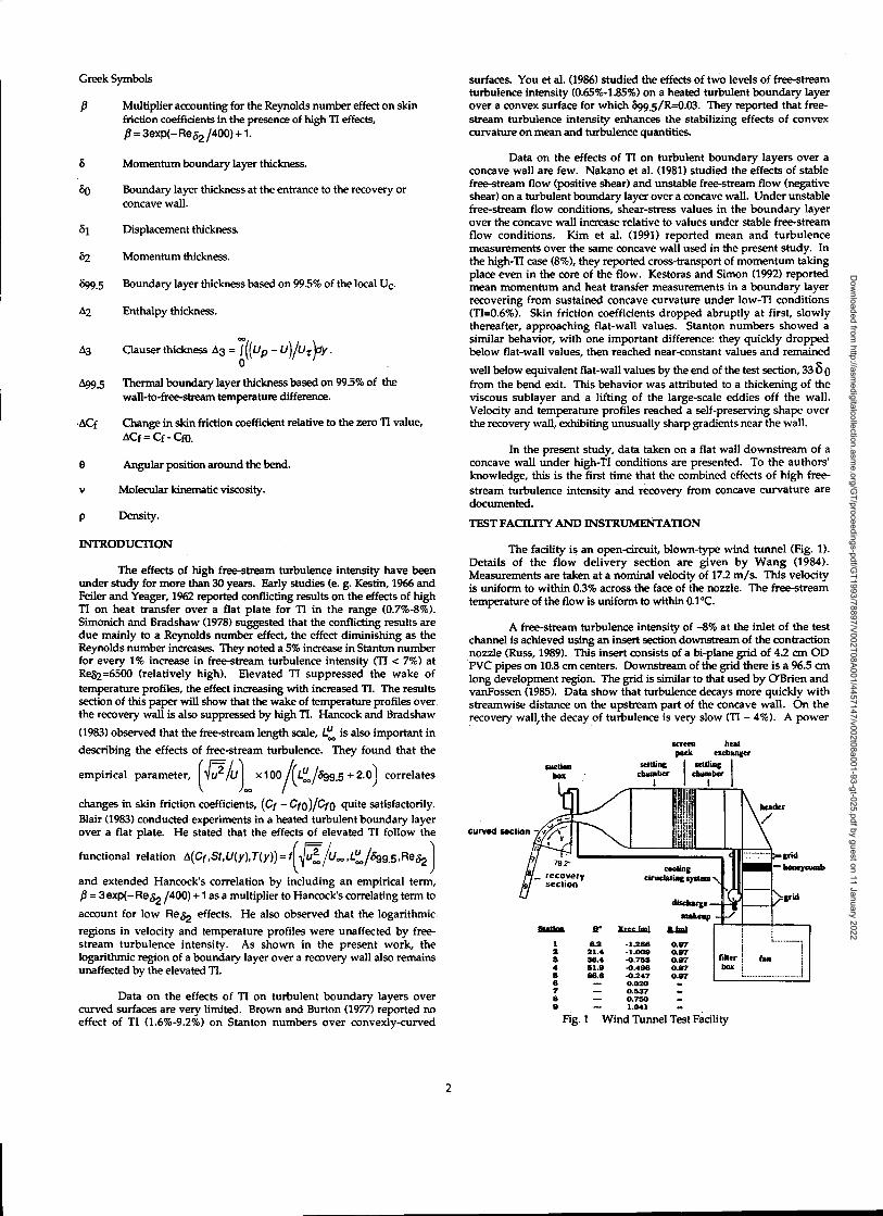
The facility is an open-circuit, blown-type wind tunnel (Fig. 1).Details of the flow delivery section are given by Wang (1984).Measurements are taken at a nominal velocity of 17.2 m/s. This velocityis uniform to within 0.3% across the face of the nozzle. The free-streamtemperature of the flow is uniform to within 0.1°C.

A free-stream turbulence intensity of —8% at the inlet of the testchannel is achieved using an insert section downstream of the contractionnozzle (Russ, 1989). This insert consists of a bi-plane grid of 4.2 cm ODPVC pipes on 10.8 cm centers. Downstream of the grid there is a 96.5 cmlong development region. The grid is similar to that used by O'Brien andvanFossen (1985). Data show that turbulence decays more quickly withstreamwise distance on the upstream part of the concave wall. On therecovery wall,the decay of turbulence is very slow (TI — 4%). A power

_Fig. 1 Wind Tunnel Test Facility

Clauser thickness A3 = ((Up — UVUr)dy.0

Thermal boundary layer thickness based on 995% of thewall-to-free-stream temperature difference.

00

2

Dow

nloaded from http://asm

edigitalcollection.asme.org/G

T/proceedings-pdf/GT1993/78897/V002T08A001/4457147/v002t08a001-93-gt-025.pdf by guest on 11 January 2022

density spectrum taken at the nozzle exit shows that 19.6% of theturbulent energy in the free-stream is distributed over frequencies whichare below 25 Hz.

The test channel is rectangular, 68 cm wide, 11 cm deep, and 284cm-long. The test wall consists of two major segments (concave wall andrecovery wall) which are designed and assembled to provide a smooth,uniformly-heated surface. Both segments were fabricated similarly. Forexample, the recovery wall consists of a layer of fiberglass insulation, asheet of Plexiglas, an electrical resistance heater, a thin spacer, a stainlesssteel sheet, and, adjacent to the flow, a layer of liquid crystal.Thermocouples embedded into the spacer are distributed both in thestreamwise and spanwise directions.

The concave wall has a radius of 0.97 m and is 1.38 m long. Therecovery wall is 1.452 m long and is tangent to the concave wall. Theouter wall is adjusted to obtain negligible streamwise acceleration: staticpressure coefficients, Cpc, are kept to within 0.03 for the entire test length.Such Cpc values are based upon static pressures taken at a radial distanceof 2 cm from the test wall. Static pressures were measured using an arrayof static pressure taps on an end wall. The taps were distributed both inthe x and y directions.

At the entry to the recovery section Rex, Re81 and Re82 are 1.4 X106, 1487 and 1174, respectively.

Data acquisition and processing are performed by a HewlettPackard series 200, Model 16 personal computer. Mean and fluctuatingvelocities are measured using a hot -wire (15I 1218-T1.5) probe on whichthe prongs are bent 90° to the probe holder to minimize flow interference.A constant-temperature, four-channel bridge (TSI-IFA-100) is used topower the hot-wires. Analog output signals are digitized using anHP3437A system voltmeter. For statistical quantities, the sampling rate is100 Hz and the sampling duration is at least 40 seconds.

Velocities are measured when the walls are not heated. The free-stream temperature is continuously monitored and the hot-wire voltageoutput is corrected for any temperature variations. The uncertainty in u2is 3%.

Heat transfer experiments are conducted with the test walls

uniformly heated to nominally 193 W / m2 within a 1% nonuniformity(Wang, 1984). Wall temperatures are measured with 76 um diameterembedded chromel-alumel thermocouples. The thermocouples werecalibrated against a platinum-resistance standard. The spacings of thethermocouples in the streamwise direction are 2.54 and 5.08 cm over theconcave and recovery walls, respectively. Surface temperatures areobtained by correcting the thermocouple readings for temperature dropsbetween the embedded thermocouple beads and the test wall surface.Such corrections for the concave and the recovery walls, respectively,were typically 1.2C and 0.3 of the 5.5*C thermocouple-to-free-streamtemperature difference. The uncertainty in the wall temperature readings,thus obtained, is 0.2°C. Careful measurements of wall materialconductivity, contact resistance values, and surface emissivity wereneeded to achieve this uncertainty. An energy balance was performed bycomparing the enthalpy thicknesses calculated from the measuredvelocity and temperature profiles and the enthalpy thicknesses obtainedby integration in the streamwise direction of wall values. On the concavewall, where the wall temperature correction is largest, a closure within 5%was obtained.

Profiles were taken using a stepping motor assembly. The motoris capable of 400 half-steps per revolution, each half-step equivalent to 5urn of travel in the y- direction.

Determination of 899.5 presents some difficulty in the high-turbulence case: no analytical equation is available for determining thevelocity distribution outside the boundary layer over the recovery wall.The velocity distribution in the core of the flow is different from thedistribution in a low-turbulence case, primarily because of cross transportof momentum by boundary work over the upstream concave wall (Eckert,

1987). Eckert suggests that this cross transport of momentum isdependent on the unsteadiness of the flow and the bending of the flowpath-lines. Both factors are nearly constant across the core of the flowover the upstream concave wall: This implies a nearly uniform crosstransport of momentum across the channel toward the concave wall butoutside the boundary layer. Though the slope of the linear distribution ofvelocities in the core of the flow over the concave wall changes from thatobserved in a low-turbulence case (Kestoras and Simon, 1992) the velocitydistribution in the core of the flow remains linear when high TI isintroduced. The velocity profile in the core of the flow throughout therecovery section also remains linear. In this work, velocities in the core ofthe flow are least-square fitted with a straight line, capitalizing on thislinearity; the resulting equation is used to provide the velocities thatwould be obtained in the vicinity of the wall if the boundary layer werenot present. The velocities, thus obtained, are used instead of Up (usedpreviously in the low-turbulence cases) to determine 899.5,451, and 82).

RESULTS

Under high free-stream turbulence conditions (TI= 8%) the flowappears fully turbulent, in terms of the wall skin friction and heat transfer,from the leading edge of the concave wall. Stable GOrtler-like vortices donot appear in the high-turbulence case, in contrast to a previous casetaken under low-TI conditions. Spanwise non-uniformities, which wouldindicate the presence of such vortices, do not appear on the liquid crystalcovering the test surface; moreover, spanwise profiles of streamwisemean velocity do not show the maxima or minima observed in the low-turbulence case. Turbulence measurements (Kestoras, 1993) indicate thata scenario whereby GOrtler-like vortices exist but meander with time maynot be correct. Indeed, it appears that there is no coherent vortex activity.The effects of high TI are most profound in the outer region of theboundary layer over the recovery wall. In the inner region, the high-TIeffects are important but the removal of concave curvature is moreinfluential.

The structural changes of the boundary layer over the upstreamconcave wall, brought about by high TI, can be described as follows: atthe bend exit, the near-wall velocity profiles exhibit sharper gradientsthan in a low-Tr case. These sharp velocity gradients are the result of thefollowing two effects taking place over the concave wall: 1) High free-stream turbulence provides large-scale, high-streamwise-momentumeddies outside the boundary layer. These eddies are accelerated towardsthe concave surface and induce an increase in eddy scale within theboundary layer. 2) Cross transport of energy by boundary work proceedseven outside of the boundary layer over the concave wall (Eckert, 1987)raising the streamwise momentum near the wall.

This paper documents the effects of the removal of concavecurvature under high-TI conditions. Measurements are presented andtheir significance discussed. Effects of TI are isolated by comparing withdata from a low-TI case (Kestoras and Simon, 1992, TI=0.6%). Importantparameters of the study are shown in Table 1.

Non-Dimensional Velocity Profiles

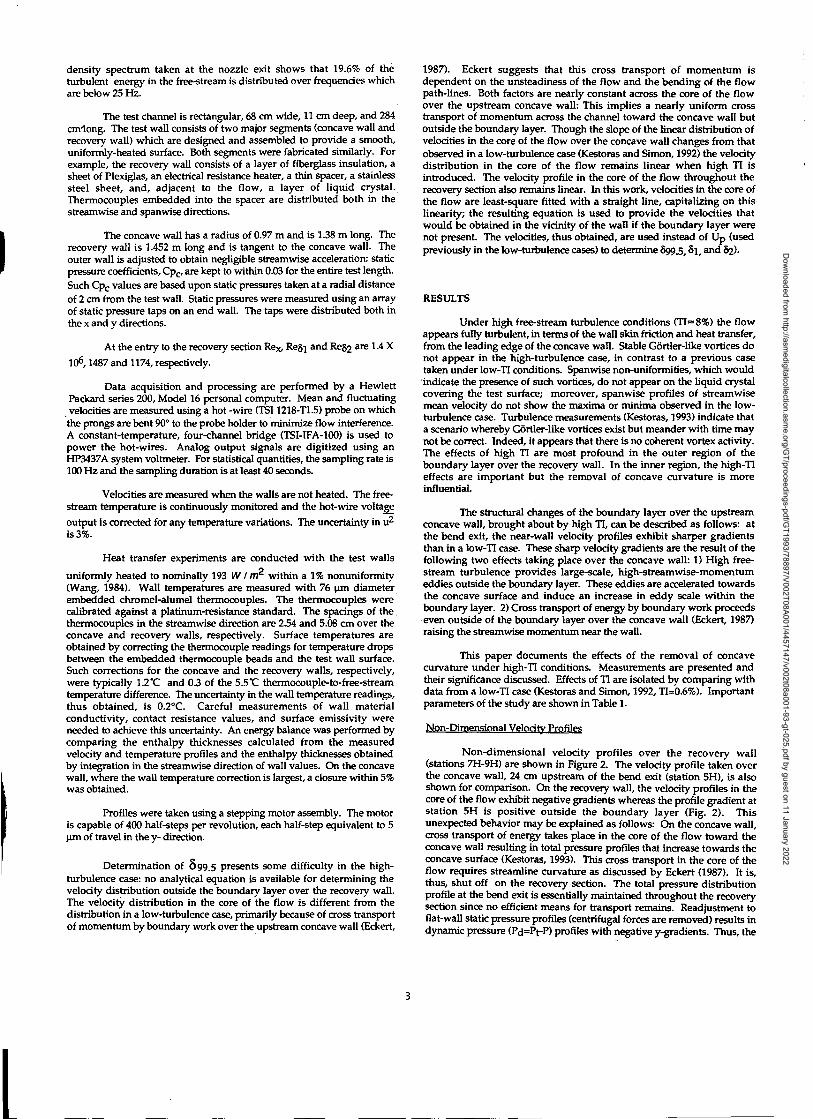
Non-dimensional velocity profiles over the recovery wall(stations 7H-9H) are shown in Figure 2. The velocity profile taken overthe concave wall, 24 cm upstream of the bend exit (station 5H), is alsoshown for comparison. On the recovery wall, the velocity profiles in thecore of the flow exhibit negative gradients whereas the profile gradient atstation 5H is positive outside the boundary layer (Fig. 2). Thisunexpected behavior may be explained as follows: On the concave wall,cross transport of energy takes place in the core of the flow toward theconcave wall resulting in total pressure profiles that increase towards theconcave surface (Kestoras, 1993). This cross transport in the core of theflow requires streamline curvature as discussed by Eckert (1987). It is,thus, shut off on the recovery section. The total pressure distributionprofile at the bend exit is essentially maintained throughout the recoverysection since no efficient means for transport remains. Readjustment toflat-wall static pressure profiles (centrifugal forces are removed) results indynamic pressure (Pd=Pt-P) profiles with negative y-gradients. Thus, the

3

Dow

nloaded from http://asm

edigitalcollection.asme.org/G

T/proceedings-pdf/GT1993/78897/V002T08A001/4457147/v002t08a001-93-gt-025.pdf by guest on 11 January 2022

..111111.111111111111111111111111111111111111111111111111111_1

Acp 43°-

-

-

-

-

-

-

-

STATION 4H --- 0 :STATION 5H --- 0 -STATION 6H

0.8

6 0.6

0.4

0.2

% e o As 2.c. °as° Qi

0.5

STATION 511 --- 0STATION 7H --- 0STATION BH --- ASTATION 9H ---

11111111111 01111111111161111011111111.MIMIIIIIIII I IIIIIIIII111111161110111110011111111111111111

2

STATION 5H --- 0STATION 7H --- 0STATION BH --- ASTATION 9H --- a

00 0.3 0.6 0.9 1.2 1.5

Y/899sFig. 2 Velocity Profiles on Recovery Wall (Stations 7H-9H). Station 5H;

Concave Wall. Profiles Shifted in the Vertical Direction

0.5

1.8

Station4H

Station5H

Station6H

Station7H

Station8H

Station9H

x (m) 0.875 1.133 1.390 1.912 2.124 2.416

R (cm) 97 97

Ucw (m/s) 16.71 17.09 16.41 17.17 16.77 16.95

T.I.core 5.201 4.631 4.618 4.150 4.135 4.127

899.5x102(m) 3.87 3.60 2.40 2.69 2.86 2.89

Six103(m) 1.987 2.129 1.452 2.052 2.308 2.473

82X103(11) 1.618 1.746 1.146 1.586 1.776 1.411

(Y/899.5)y+.1 0 0.006 0.005 0.008 0.007 0.007 0.007

Re. x105 9.44 12.05 14.23 20.84 23.26 25.68

Rest 2144 2264 1487 2236 2527 2630

Re82 1746 1857 1174 1728 1944 2033

1.228 1.219 1.267 1.294 1.300 1.294

Cfx103 5.00 4.93 4.85 4.45 4.36 4.19

(aU /ay)core 10.1 15.4 15.7 -10.1 -9.5 -9.6

99.5(cm) 3.312 4.538 6.062 6.157 7.693 8.817

2(tran) 1.602 2.372 2.478 2.304 4.042 4.104

27.74 27.77 27.74 27.68 27.60 27.67

T(c) 31.32 31.35 31.74 31.94 31.88 32.13

ReA2 1662 2517 2521 2451 4203 4310

qw 165.6 165.4 172.1 163.8 163.6 162.6

St x103 2.376 2.321 2.251 1.922 1.957 1.846

2 St/C1 0.951 0.941 0.928 0.864 0.898 0.881

Table 1. Boundary Layer Parameters. Concave-Wall Stations 4H and5H; Joint: Station 6H; Recovery wall Stations 7H-9H.

velocity profile ( Pd == 0.5pU2) also exhibits a negative y-gradient.

After the removal of curvature, the boundary layer thicknesses,899.5, 81 and 82 decrease (Station 7H in Table 1). Values of 899.5, 61 and82 increase monotonically for the rest of the recovery wall. Their valueshowever, do not rise above the pre bend-exit value (station 5H) before themid-downstream location of the recovery wall (station 8H). It thereforeappears that there is a mechanism in the vicinity of the bend exit whichtransports streamwise momentum away from the wall quite efficiently.Before the bend exit (station 5H in Fig. 2) streamwise momentumincreases with y. By conservation of angular momentum, the fluid layerswith the higher streamwise momentum may tend to lift off the test wallwhereas fluid layers close to the surface show a smaller tendency to liftoff. This impulse of cross transport of momentum away from the testwall in the vicinity of the bend exit is consistent with the readjustment ofthe shape of the local velocity profiles. At the joint between the concaveand recovery walls (station 6H), the near-wall, y/899.5 <0.03 velocitygradient, is shallower than for the upstream profiles (stations 4H and 5Hin Fig. 3). This may at first seem strange since readjustment of staticpressure profiles would tend to produce near-wall acceleration at thispoint. It is believed to be a result of the lifting of the vortices.

As with the low-TI case, the recovery wall velocity profilesassume a near-asymptotic shape (stations 7H-9H in Fig. 4). This behavioris especially true near the wall y/899.5 < 0.13. Moreover, near the wall(y/899.5 <0.13), self-similarity is established by station 6H (only 2 cmdownstream of the bend exit, not shown in the Fig. 4) suggesting that theredistribution of momentum discussed above begins slightly upstream ofthe bend exit and is complete soon after the beginning of recovery.

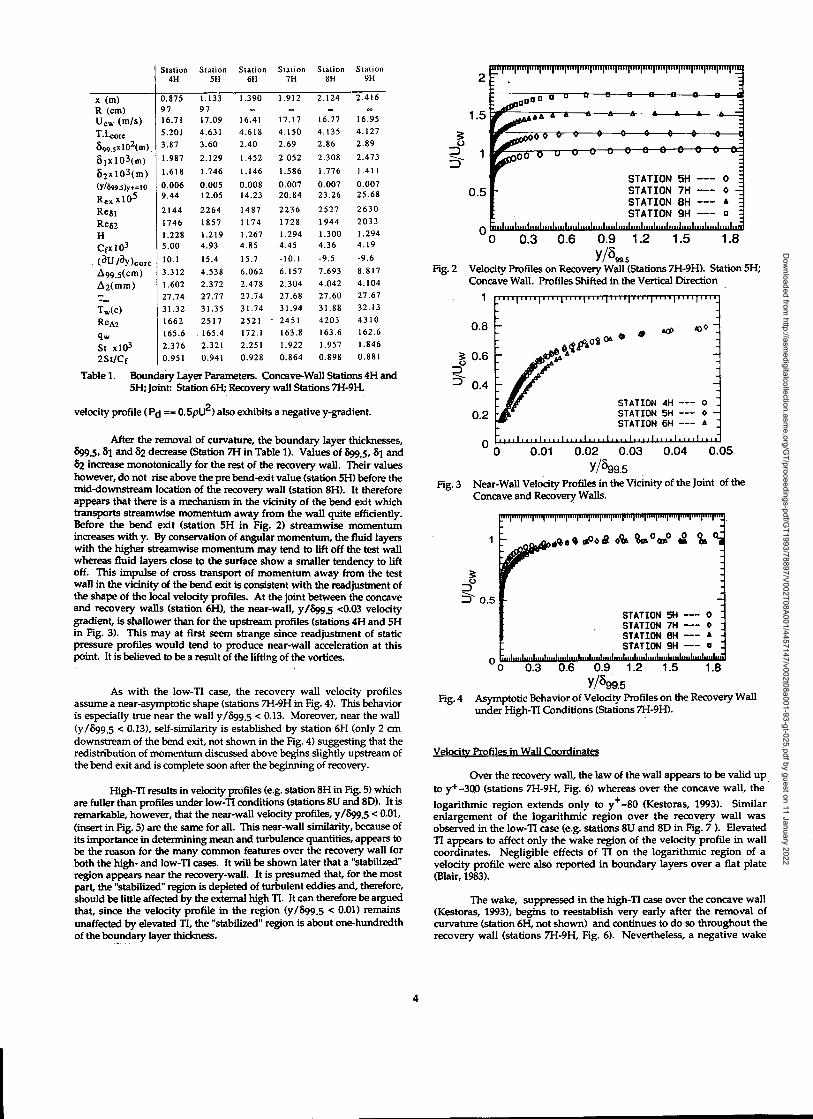
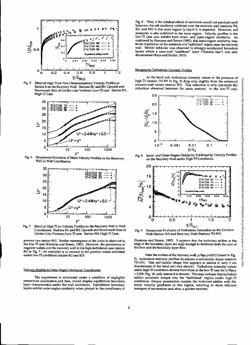
High-TI results in velocity profiles (e.g. station 8H in Fig. 5) whichare fuller than profiles under low-TI conditions (stations 8U and 8D). It isremarkable, however, that the near-wall velocity profiles, y/899.5 < 0.01,(insert in Fig. 5) are the same for all. This near-wall similarity, because ofits importance in determining mean and turbulence quantities, appears tobe the reason for the many common features over the recovery wall forboth the high- and low-TI cases. It will be shown later that a "stabilized"region appears near the recovery-wall. It is presumed that, for the mostpart, the "stabilized" region is depleted of turbulent eddies and, therefore,should be little affected by the external high TI. It can therefore be arguedthat, since the velocity profile in the region (y/899.5 <0.01) remainsunaffected by elevated TI, the "stabilized" region is about one-hundredthof the boundary layer thickness.

..11111111,1111111111,11111111,11"111111111111111111,111111:

0.01 0.02 0.03 0.04

0.05

y/899.5Fig. 3 Near-Wall Velocity Profiles in the Vicinity of the Joint of the

Concave and Recovery Walls.

0.3 0.6 0.9 1.2 1.5 1.8Y/899.5

Fig. 4 Asymptotic Behavior of Velocity Profiles on the Recovery Wallunder High-TI Conditions (Stations 7H-9H).

Velocity Profiles in Wall Coordinates

Over the recovery wall, the law of the wall appears to be valid upto y+-3()0 (stations 7H-9H, Fig. 6) whereas over the concave wall, thelogarithmic region extends only to y+.-80 (Kestoras, 1993). Similarenlargement of the logarithmic region over the recovery wall wasobserved in the low-TI case (e.g. stations 8U and 8D in Fig. 7). ElevatedTI appears to affect only the wake region of the velocity profile in wallcoordinates. Negligible effects of TI on the logarithmic region of avelocity profile were also reported in boundary layers over a flat plate(Blair, 1983).

The wake, suppressed in the high-TI case over the concave wall(Kestoras, 1993), begins to reestablish very early after the removal ofcurvature (station 6H, not shown) and continues to do so throughout therecovery wall (stations 7H-9H, Fig. 6). Nevertheless, a negative wake

0 0

4

Dow

nloaded from http://asm

edigitalcollection.asme.org/G

T/proceedings-pdf/GT1993/78897/V002T08A001/4457147/v002t08a001-93-gt-025.pdf by guest on 11 January 2022

1 1 115.1 1

: STATION 7H +

=STATION BH *STATION 9H ---

10 100 1000y+

Fig. 6 Streamwise Evolution of Mean Velocity Profiles on the RecoveryWall in Wall Coordinates.

1111 1 1151111 1

STATION BD --- + -STATION BU *STATION BH

35 -

30 E-25

20

10 E- li*--2441ny++5.0- -=:

5...- U+=y+ .z.

0 ' 1 10 100 1000

STATION 7H +STATION 8H --- *STATION 9H ---

4101AWObsalo

STATION 5HSTATION 7HSTATION SHSTATION 9H

Expamkdy4993.uk

A A A A„ op 0 0* P 0 0

°O16 s' .•■•■■•...1.'••■"•'1••^1"."'Irr`TI'•"1••'•1••••

• 0:0.6- ek, o•-

STATION 80 --- 0v 0.4 STATION 8U o -

STATION 8H --- A

0.2Expanded y/b99.5-scale

0 0.01 0.02 0.03 0.04 0.05 y/99.5

0.2 0.4 0.6 0.8

12

099.5Fig. 5 Effect of High TI on Non-Dimensionalized Velocity Profiles at

Station Son the Recovery Wall. Stations 8U and 8D; Upwash andDownwash Sites of GOrtler-Like Vortices-Low-TI case. Station 8H;High-TI Case.

y+Fig. 7 Effect of High TI on Velocity Profiles on the Recovery Wall in Wall

Coordinates. Stations 8U and 8D; Upwash and Downwash Sites ofGfirtler-Like Vortices-Low-TI case. Station 8H; High-TI Case.

persists (see station 9H). Similar reemergence of the wake is observed inthe low-TI case (Kestoras and Simon, 1992). However, the persistence ofnegative wakes over the recovery wall in the high-turbulence case (station8H in Fig. 7, for example) is in contrast to the positive wakes exhibitedunder low-TI conditions (station 8U and 8D).

Velocity Profiles in Outer-Region Similarity Coordinates

The experiment is conducted under a condition of negligiblestreamwise acceleration and thus, would display equilibrium boundarylayer characteristics under flat-wall conditions. Equilibrium boundarylayers exhibit outer-region similarity when plotted in the coordinates of

Fig. 8. Thus, if the residual effects of curvature would not preclude suchbehavior, the self similarity exhibited over the recovery wall (stations 7H,8H, and 9H) in the outer region (y/A3>0.1) is expected. However, selfsimilarity is also exhibited in the inner region. Velocity profiles in thelow-TI case also exhibit both inner- and outer-region similarity. Asexplained by Kestoras and Simon (1992), this inner-region similarity maybe an implication of the existence of a "stabilized" region near the recoverywall. Similar behavior was observed in strongly-accelerated boundarylayers where a near-wall "stabilized" layer ("laminar-like") was alsodocumented (Kays and Moffat, 1975).

Streamwise Turbulence Intensity Profiles

At the bend exit, turbulence intensity values in the presence ofhigh TI (station 7H-9H in Fig. 9) drop only slightly from the enhancedconcave-wall values (station 5H). This reduction is only one-tenth thereduction observed between the same stations in the low-TI case

0.001 0.01

0.1

103

Fig. 8 Inner- and Outer-Region Similarity Exhibited by Velocity Profileson the Recovery Wall under High-TI Conditions.

Fig. 9 Streamwise Evolution of Turbulence Intensities on the ConcaveWall (Station 5H) and Recovery Wall (Stations 7H-9H).

(Kestoras and Simon, 1992). It appears that the turbulent eddies at theedge of the boundary layer are large enough to dominate both the core ofthe flow and the boundary layer flow.

Near the surface of the recovery wall, y/899.5<0.012 (insert in Fig.9), turbulence intensity profiles do assume a self-similar shape (stations7H-9H). This self-similar shape first appears at station 6, only 2 cmdownstream of the bend exit (not shown). Turbulence intensity valuesunder high-TI conditions deviate from those in the low-TI case for y/899.5>0.006 (Fig. 10, only station 8 is shown). This may indicate that turbulenteddies penetrate deeper into the "stabilized" region under high-TIconditions. Deeper penetration couples the turbulent eddies with thesharp velocity gradients in this region, resulting in more efficienttransport of momentum and, thus, a quicker recovery.

O.5

1 o4

5

Dow

nloaded from http://asm

edigitalcollection.asme.org/G

T/proceedings-pdf/GT1993/78897/V002T08A001/4457147/v002t08a001-93-gt-025.pdf by guest on 11 January 2022

1 6

1 4

1 2a- 1 0

STATION 80 ---STATION 8U --- 0STATION 8H --- A

00 0.01 0.02 0.03

y/899.5Fig. 10 Effect of High TI on Near-Wall Turbulence Intensities on the

Recovery Wall. Stations 8U and 8D; Upwash and Downwash Sitesof GOrtler-Like Vortices-Low-TI case. Station 8H; High-TI Case.

E`,4

0.05

STATION 7H ---STATION 8H --- 0STATION 9H --- A

' ' ' ' ""I I ' ' ' ""ISTATION 5H +STATION 6H --- *STATION 7H ---STATION 8H --- oSTATION 9H ---

CI

50

40

30

1-1- 20

10

1000

it STATION 80 ---STATION 8U ---STATION 8H ---

Expanded ythapls-scale

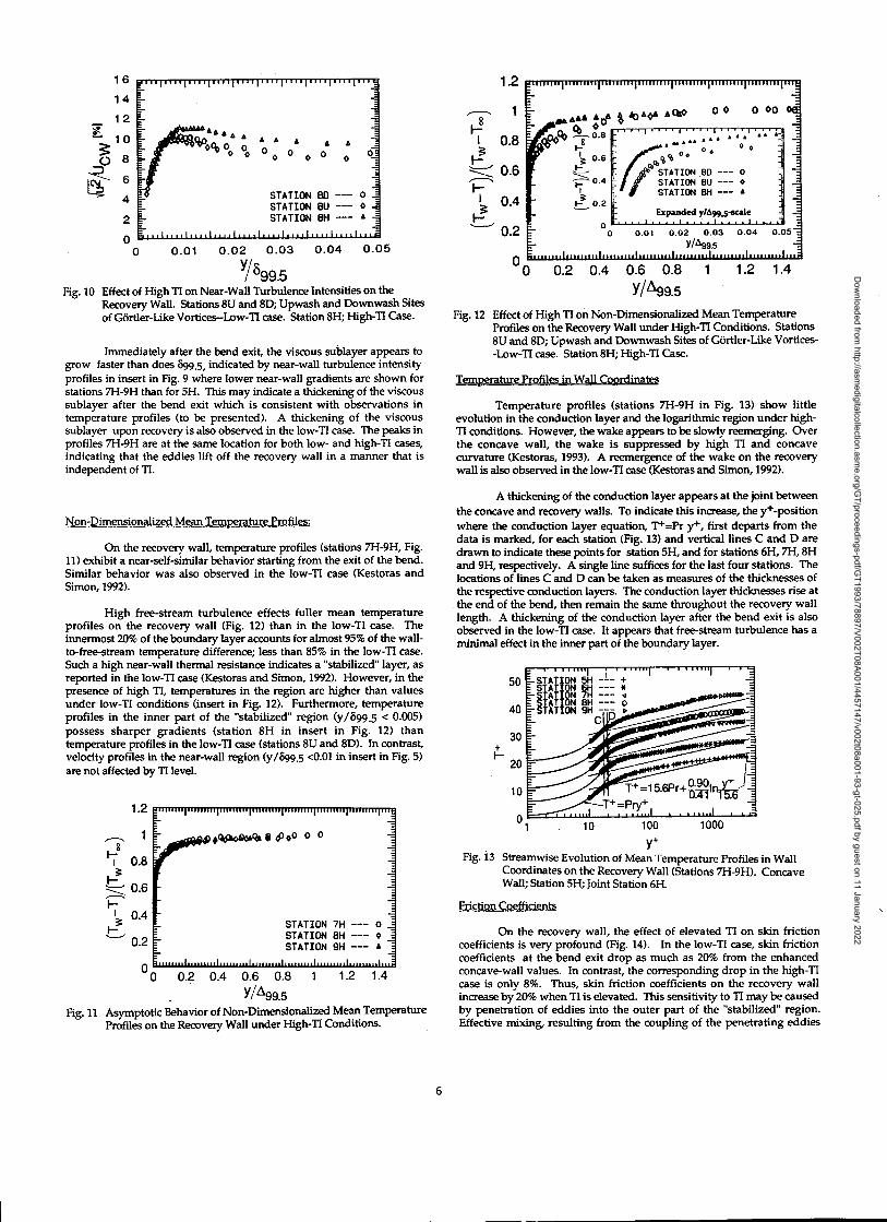
Immediately after the bend exit, the viscous sublayer appears togrow faster than does 599.5, indicated by near-wall turbulence intensityprofiles in insert in Fig. 9 where lower near-wall gradients are shown forstations 7H-9H than for 5H. This may indicate a thickening of the viscoussublayer after the bend exit which is consistent with observations intemperature profiles (to be presented). A thickening of the viscoussublayer upon recovery is also observed in the low-TI case. The peaks inprofiles 7H-9H are at the same location for both low- and high-TI cases,indicating that the eddies lift off the recovery wall in a manner that isindependent of TI.

Non-Dimensionalized Mean Temperature Profiles:

On the recovery wall, temperature profiles (stations 7H-9H, Fig.11) exhibit a near-self-similar behavior starting from the exit of the bend.Similar behavior was also observed in the low-TI case (Kestoras andSimon, 1992).

High free-stream turbulence effects fuller mean temperatureprofiles on the recovery wall (Fig. 12) than in the low-TI case. Theinnermost 20% of the boundary layer accounts for almost 95% of the wall-to-free-stream temperature difference; less than 85% in the low-TI case.Such a high near-wall thermal resistance indicates a "stabilized" layer, asreported in the low-TI case (Kestoras and Simon, 1992). However, in thepresence of high TI, temperatures in the region are higher than valuesunder low-TI conditions (insert in Fig. 12). Furthermore, temperatureprofiles in the inner part of the "stabilized" region (y/599.5 < 0.005)possess sharper gradients (station 8H in insert in Fig. 12) thantemperature profiles in the low-TI case (stations 8U and 8D). In contrast,velocity profiles in the near-wall region (y/599,5 <0.01 in insert in Fig. 5)are not affected by TI level.

Y/1199.5Fig. 11 Asymptotic Behavior of Non-Dimensionalized Mean Temperature

Profiles on the Recovery Wall under High-TI Conditions.

00 0.2 0.4 0.6 0.8 1

Y/A99.5

Fig. 12 Effect of High TI on Non-Dimensionalized Mean TemperatureProfiles on the Recovery Wall under High-TI Conditions. Stations8U and 8D; Upwash and Downwash Sites of GOrtler-Like Vortices--Low-TI case. Station 8H; High-TI Case.

Temperature Profiles in Wall Coordinates

Temperature profiles (stations 7H-9H in Fig. 13) show littleevolution in the conduction layer and the logarithmic region under high-TI conditions. However, the wake appears to be slowly reemerging. Overthe concave wall, the wake is suppressed by high TI and concavecurvature (Kestoras, 1993). A reemergence of the wake on the recoverywall is also observed in the low-TI case (Kestoras and Simon, 1992).

A thickening of the conduction layer appears at the joint betweenthe concave and recovery walls. To indicate this increase, the y+-positionwhere the conduction layer equation, T+=Pr y+, first departs from thedata is marked, for each station (Fig. 13) and vertical lines C and D aredrawn to indicate these points for station 5H, and for stations 6H, 7H, 8Hand 9H, respectively. A single line suffices for the last four stations. Thelocations of lines C and D can be taken as measures of the thicknesses ofthe respective conduction layers. The conduction layer thicknesses rise at

• the end of the bend, then remain the same throughout the recovery walllength. A thickening of the conduction layer after the bend exit is alsoobserved in the low-TI case. It appears that free-stream turbulence has aminimal effect in the inner part of the boundary layer.

Fig. 13 Streamwise Evolution of Mean Temperature Profiles in WallCoordinates on the Recovery Wall (Stations 7H-9H). ConcaveWall; Station 5H; Joint Station 6H.

Friction Coefficients

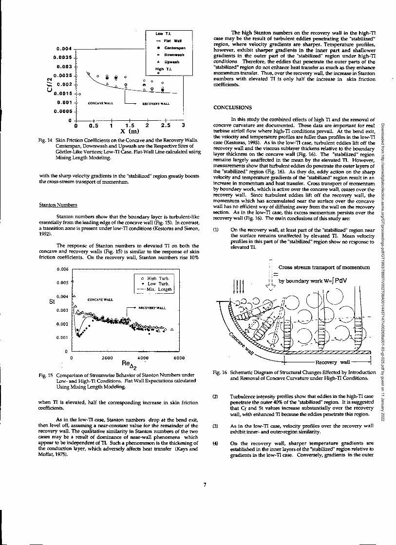
On the recovery wall, the effect of elevated TI on skin frictioncoefficients is very profound (Fig. 14). In the low-TI case, skin frictioncoefficients at the bend exit drop as much as 20% from the enhancedconcave-wall values. In contrast, the corresponding drop in the high-TIcase is only 8%. Thus, skin friction coefficients on the recovery wallincrease by 20% when TI is elevated. This sensitivity to TI may be causedby penetration of eddies into the outer part of the "stabilized" region.Effective mixing, resulting from the coupling of the penetrating eddies

1.2

1

I 0.8

0.6

0.4

0.2

1.2 1.4

6

Dow

nloaded from http://asm

edigitalcollection.asme.org/G

T/proceedings-pdf/GT1993/78897/V002T08A001/4457147/v002t08a001-93-gt-025.pdf by guest on 11 January 2022

0.001

0.006

0.005

0.004St

0.003

0.002

• High Turb.• Low Turb.

—Mix. Length

Recovery wall ---I

Fig. 16 Schematic Diagram of Structural Changes Effected by Introductionand Removal of Concave Curvature under High-TI Conditions.

Low

— Flat Wan

• Centerspan

o Downwash

a Upwash

High 1.1.

0 0.5 1 1.5 2

2 . 5

3X(m)

Fig. 14 Skin Friction Coefficients on the Concave and the Recovery Walls.Centerspan, Downwash and Upwash are the Respective Sites ofGiirtler-Like Vortices; Low-TI Case. Flat-Wall Line calculated usingMixing Length Modeling.

with the sharp velocity gradients in the "stabilized" region greatly booststhe cross-stream transport of momentum.

Stanton Numbers

Stanton numbers show that the boundary layer is turbulent-likeessentially from the leading edge of the concave wall (Fig. 15). In contrast,a transition zone is present under low-TI conditions (Kestoras and Simon,1992).

The response of Stanton numbers to elevated TI on both theconcave and recovery walls (Fig. 15) is similar to the response of skinfriction coefficients. On the recovery wall, Stanton numbers rise 10%

0 2000

4000

6000Re

6,2Fig. 15 Comparison of Streamwise Behavior of Stanton Numbers under

Low- and High-TI Conditions. Flat Wall Expectations calculatedUsing Mixing Length Modeling.

when TI is elevated, half the corresponding increase in skin frictioncoefficients.

As in the low-TI case, Stanton numbers drop at the bend exit,then level off, assuming a near-constant value for the remainder of therecovery wall. The qualitative similarity in Stanton numbers of the twocases may be a result of dominance of near-wall phenomena whichappear to be independent of TI. Such a phenomenon is the thickening ofthe conduction layer, which adversely affects heat transfer (Kays andMoffat, 1975).

The high Stanton numbers on the recovery wall in the high-TIcase may be the result of turbulent eddies penetrating the "stabilized"region, where velocity gradients are sharper. Temperature profiles,however, exhibit sharper gradients in the inner part and shallowergradients in the outer part of the "stabilized" region under high-TIconditions Therefore, the eddies that penetrate the outer parts of the"stabilized" region do not enhance heat transfer as much as they enhancemomentum transfer. Thus, over the recovery wall, the increase in Stantonnumbers with elevated TI is only half the increase in skin frictioncoefficients.

CONCLUSIONS

In this study the combined effects of high TI and the removal ofconcave curvature are documented. These data are important for realturbine airfoil flow where high-TI conditions prevail. At the bend exit,the velocity and temperature profiles are fuller than profiles in the low-TIcase (Kestoras, 1993). As in the low-TI case, turbulent eddies lift off therecovery wall and the viscous sublayer thickens relative to the boundarylayer thickness on the concave wall (Fig. 16). The "stabilized" regionremains largely unaffected in the mean by the elevated TI. However,measurements show that turbulent eddies do penetrate the outer layers ofthe "stabilized" region (Fig. 16). As they do, eddy action on the sharpvelocity and temperature gradients of the "stabilized" region result in anincrease in momentum and heat transfer. Cross transport of momentumby boundary work, which is active over the concave wall, ceases over therecovery wall. Since turbulent eddies lift off the recovery wall, themomentum which has accumulated near the surface over the concavewall has no efficient way of diffusing away from the wall on the recoverysection. As in the low-TI case, this excess momentum persists over therecovery wall (Fig. 16). The main conclusions of this study are:

(1) On the recovery wall, at least part of the "stabilized" region nearthe surface remains unaffected by elevated TI. Mean velocityprofiles in this part of the "stabilized" region show no response toelevated TI.

Cross stream transport of momentum

(2) Turbulence intensity profiles show that eddies in the high-TI casepenetrate the outer 40% of the "stabilized" region. It is suggestedthat Cf and St values increase substantially over the recoverywall, with enhanced TI because the eddies penetrate this region.

(3) As in the low-TI case, velocity profiles over the recovery wallexhibit inner- and outer-region similarity.

(4) On the recovery wall, sharper temperature gradients areestablished in the inner layers of the "stabilized" region relative togradients in the low-TI case. Conversely, gradients in the outer

0.004

0.0035 —

0.003 4

0.0025—

0.002

0.0015 4o

0.001 4 CONCAVE WALL

0.0005 4

0

0 0

RECOVERY WALL

7

Dow

nloaded from http://asm

edigitalcollection.asme.org/G

T/proceedings-pdf/GT1993/78897/V002T08A001/4457147/v002t08a001-93-gt-025.pdf by guest on 11 January 2022

part of the "stabilized" region are reduced. Thus the effectivenessof the mixing resulting from the eddies penetrating the outerparts of the "stabilized" region is reduced. As a result, heattransfer on the recovery wall does not increase with increased TIas much as does momentum transfer.

(5) The boundary layer over the recovery wall appears to be free ofspanwise non-uniformities. It is suggested that G8rtler-likevortices do not form under high-TI conditions.

(6) For y+ <300, the momentum law of the wall remains valid overthe recovery wall.

ACKNOWLEDGMENTSThis work was supported by the Air Force Office of Scientific

Research. The project (grant number AF/AFOSR-91-0322) monitor is Maj.D. Pant.

REFERENCES

Blair, M. F., (1983), "Influence of Free-Stream Turbulence on TurbulentBoundary Layer Heat Transfer and Mean Profile Development, Part II-Analysis of Results", J. of Heat Transfer, Vol. 105, pp.41-47.

Brown, A., and Burton, R. C., (1977), 'The Effects of Free-StreamTurbulence Intensity and Velocity Distribution on Heat Transfer toCurved Surfaces", ASME Paper 77-Gt-48.

Eckert E. R. G., (1987), "Cross Transport of Energy in Fluid Streams,"Wärme-und Stoffiibertragung, Vol. 21, pp. 73-81.

Feiler, C.E. and Yeager, E.B., (1962), "Effect of Large-AmplitudeOscillations on Heat Transfer", NASA Tech. Report R-142, 1962.

Hancock, P. E., and Bradshaw, P., (1983), 'The Effect of Free-StreamTurbulence on Turbulent Boundary Layers", Transactions of the ASME,Vol. 105, pp. 284-289.

Kays, W.M., and Moffat, R.J. (1975) "The Behavior of TranspiredTurbulent Boundary Layers", Report HMT-20, Thermosciences Division,Department of Mechanical Engineering, Stanford University.

Kestin, J., (1966), "The Effects of Free-Stream Turbulence on Heat TransferRates", Advances in Heat Transfer, Vol. 3, ed. by T.F. Irvine, Jr. and J.P.Hartnett, Academic Press, London 1966.

Kestoras, M.D., and Simon, T.W., (1992), "Hydrodynamic and ThermalMeasurements in a Turbulent Boundary Layer Recovering from ConcaveCurvature," ASME Journal of Turbomachinety, Vol. 114, No. 4, pp. 891-898.

Kestoras, M.D. (1993), "Heat Transfer and Fluid Mechanics Measurementsin a Turbulent Boundary Layer Recovering from Concave Curvature",Ph.D. Thesis, University of Minnesota.

Kim, J., Simon, T.W., and Russ, S.G., (1991), "Free-stream Turbulence andConcave Curvature Effects on Heated, Transitional Boundary Layers,"ASME J. of Heat Transfer, Vol. 114, No. 2, pp. 339-347.

Nakano, S., Takahashi, A., Shizawa, T. and, Honami, S., (1981), "Effects ofStable and Unstable Free-Streams on a Turbulent Flow Over a ConcaveSurface", Proc. 3rd Symposium on Turbulent Shear Flows, Davis, CA.

O'Brien, J.E. and vanFossen, G.J. (1985) "The Influence of Jet GridTurbulence on Heat Transfer from the Stagnation region of a Cylinder inCross Flow", ASME 85-HT-58.

Russ, S.G. (1989), "The Generation and Measurement of Turbulent FlowFields", MSME Thesis, Dept of Mech, Engin., University of Minnesota.

Simonich, J. C., and Bradshaw, P., (1978), "Effect of Free-StreamTurbulence on Heat Transfer through a Turbulent Boundary Layer",Transactions of the ASME, Vol. 100, pp. 671-677.

Wang, T., (1984), "An Experimental Investigation of Curvature andFreestream Turbulence Effects on Heat Transfer and Fluid Mechanics inTransition Boundary Layer Flows," PhD Thesis, University of Minnesota.

You, S. M., Simon, T. W., and Kim, J., (1986), "Free-Stream TurbulenceEffects on Convex-Curved Turbulent Boundary Layers", Proc. GasTurbine Heat Transfer Session, ASME Winter Annual Meeting.

8

Dow

nloaded from http://asm

edigitalcollection.asme.org/G

T/proceedings-pdf/GT1993/78897/V002T08A001/4457147/v002t08a001-93-gt-025.pdf by guest on 11 January 2022