QINETIQ/07/01953 (AIAA-2007-3632)1 www.QinetiQ.com

Some Observations on the Noise of Heated Jets

Marcus Harper-BourneQINETIQ/07/01953July 2007

Originally, presentation AIAA-2007-3632, 13th AIAA/CEAS Aeroacoustics Conference 21-23 May 2007, Rome, Italy

QINETIQ/07/01953 (AIAA-2007-3632)2

Some Observations on the Noise of Heated Jets

Marcus Harper-Bourne.1QinetiQ, England

In the past much of our fundamental knowledge of jet noise has been acquired experimentally through tests on unheated static jets. However, an understanding of the noise of the hot exhausts that characterize jet aircraft in flight is essential to the aero-industry for research and noise certification purposes. In this paper, the effect of jet temperature on subsonic jet mixing noise is studied at model scale with an 86mm diameter convergent nozzle both statically and under simulated flight conditions. The fundamental test data used in the study was obtained in 1983 in the large-scale anechoic environment of the QinetiQ Noise Test Facility at Farnborough. Using this legacy data, jet temperature ratios ranging from isothermal to max engine core temperature are investigated over a range of velocities, enabling the temperature dependence of the noise spectrum at constant velocity to be studied and analyzed. Using Lighthill’s theory for guidance, a semi-empirical analysis of the results is undertaken that confirms the existence of entropy noise in heated jets. Master spectra for the momentum and entropy noise components are determined from the measurements and the dipole nature of the entropy component, originally proposed by Morfey, is verified. The behavior of the momentum and entropy noise under simulated flight conditions is also investigated, with the aid of an alternative approach to the modelling of flight effect.

Nomenclaturea0 = ambient speed of soundCP = specific heat of air at constant pressure (J/kg)D = nozzle diameter (m)Dp = non-dimensional overall directivity factorDf = Doppler factor θcos1 cM−δ = kronecker deltaE = dipole entropy strengthf = frequency (Hz)γ = ratio of specific heatsG = 1/3rd octave level (Pa2)HRE,EN = master spectrum of Reynolds and entropy noiseK = shear layer density fractionKRE,EN = non-dimensional source constantMj = jet fully expanded Mach numberOASPL = overall sound pressure levelp = local instantaneous pressure (Pa)P = power spectral density (Pa2/Hz)pjTOT = total pressure of jet (Pa)r0 = microphone polar radius (m)R = gas constant 287.1 J/kgρ = effective average source gas density (kg/m3)ρ0 = ambient density (kg/m3)ρj = density of the jet in the potential core (kg/m3)S = entropy (J/kg)SPL = 1/3rd octave sound pressure level (rel. 20µPa)T0 = ambient temperature

1 QinetiQ Technical Fellow, mhbourne@qinetiq.com, AIAA Member.

Copyright © 2007 by the author. Published with permission.

QINETIQ/07/01953 (AIAA-2007-3632)3

Tj = fully expanded static temperature in the potential core of the jetTjTOT = total temperature of jetTR = ratio of jet static temperature to ambient temperatureθ = polar angle relative to jet axisu = local instantaneous flow velocity (m/s)Vj, Uj = fully expanded jet velocity (m/s)VR = ratio of fully expanded jet velocity ratio to ambient speed of sound (acoustic Mach number)

I. IntroductionWith the advent of the jet engine over 50 years ago, research into jet noise began in earnest. Experimental studies

at both model and full scale by scientific bodies such as the NACA1-3, institutes of learning4 and the aero industry5, laid the initial foundations to which Lighthill provided a scientific basis in 1952 through his theory of noise generated aerodynamically6-8. The early experimental work established that small-scale laboratory jets, with their moderate Reynolds numbers, provided useful turbulence and noise measurements for the study and suppression of jet engine noise9. However, while many developments and advances in aeroacoustics have taken place since those days, fundamental problems in the understanding of jet noise identified during the seventies10 still exist, such as flight effect and the effect of jet temperature, to mention but two. After being played down for many years, the importance of temperature in the numerical/analytical study of jet noise generation is now gathering momentum11-17

and the time is now right to review the experimental database against which such studies need to perform.Over the years many experimental studies (too numerous to list) have been made on the mixing noise of heated

jets, often with different results. However, that jet noise is inherently difficult to measure with any certain accuracy is well known, particularly for heated jets where rig noise can be an issue. With the development of improved jet noise test facilities18-22, renewed interest in temperature effect is justified on this basis alone

In this paper we therefore return to the question of what effect does the temperature of a jet actually have on jet mixing noise and attempt to ascribe physical understanding to our observations. The general consensus of experimentalists, as noted by Tanner23 and Cocking24, is that the noise of a heated jet is higher at low velocities (< 0.7a0) than that of an unheated jet of the same velocity. However this observation is based on noise measurements made using small nozzles, typically 10% or less the size of actual engine exhaust nozzles. In a recent study of the noise of heated subsonic model-scale jets, Vishwanathan25 concluded that the noise increase associated with jet temperature is attributable to the Reynolds number of the jet, which reduces as the temperature is increased and therefore makes smaller nozzles more prone to exhibit this effect. As applied research into jet noise is mostly carried out at model-scale, such a conclusion, if generally true, could have serious implications for jet noise research.

The current paper is based on the examination and analysis of a comprehensive series of fundamental subsonic jet noise measurements that were made in 1983 on a single-stream 86mm (3.4 inch) convergent nozzle. The measurements were made in the QinetiQ large anechoic Noise Test Facility (NTF), at what was then the Royal Aircraft Establishment. This unique test programme, which included both static and flight simulation, was funded by the United Kingdom Department of Trade and Industry, under the Civil Aircraft Research And Development (CARAD) programme. The jet noise measurements were made over a range of fully expanded jet velocities and static temperatures compatible with those of aero-engine exhausts, for flight stream speeds between 0 and 100m/s. These tests were originally described by Bryce26 in an analysis of flight effect. The results for the static tests have subsequently been made available as legacy data for download through the QinetiQ web site in the form of Excel® spreadsheets as described by Pinker27.

Using this unique data set, a semi-empirical study of temperature effect is made employing Lighthill’s theory6

for guidance, in conjunction with Morfey’s dipole theory28 to separate entropy and momentum stress noise components. To provide a starting point, the study is restricted to the analysis of the noise at 90 degrees to the jet axis, where the effect of temperature can be studied essentially in isolation from refraction and convection effects. From the static noise measurements, master spectra for the two noise components are determined and the flight data is then used to investigate their dependence on forward flight. For the estimation of flight effect, an alternative intuitive approach is introduced in this work.

II. Basic Theory

In order to obtain a basic insight we start with Lighthill’s theory of sound generated aerodynamically6-8 in which for a free jet the source term is the second time derivative of the Lighthill stress tensor ijT . Neglecting viscous

contributions, it is well known that ijT is comprised of two main terms: a Reynolds stress jiuuρ and an entropy

QINETIQ/07/01953 (AIAA-2007-3632)4

term ijap δρ}{ 20− associated with the non-isentropic behaviour of turbulence. In unheated jets only the Reynolds

term is considered to be important whereas in heated jets, as well as the momentum transfer associated with theReynolds stress, we must also consider entropy transfer across the shear layer.

For this study, Lighthill’s retarded time integral6 for the far-field pressure fluctuation is best expressed in the less complex but equally correct form after Proudman29:

[ ] dVTra

typv

rr∫= &&0

204

1),ˆ(π

(1)

in which }{ 20

2 ρρ apuT rrr −+= (2)and ru is the instantaneous velocity resolved in the direction of the microphone/observer.Equation (1) is readily confirmed upon evaluating the double summation of the stress tensor weighted by the

product of direction cosines jicc , in Lighthill’s integral, when we then obtain:

rr

i j

ijji TTcc∑∑ = (3)

In this form, the source term, equation (2), is seen to equal the sum of the vector 2ruρ - equal to the Reynolds

stress in the direction of the microphone and the scalar }{ 20 ρap − , which by definition is omnidirectional.

A. Quadrupole NoiseRestricting attention to 2

ruρ in equation (1), we start by applying the usual dimensional similarity arguments,

namely, that Reynolds stress 2jVρ∝ , characteristic frequency DV j /∝ , and volume 3D∝ . Then, ignoring

fluctuations in the density ρ , we obtain the momentum or quadrupole contribution to the intensity of the sound in

the classical 8V form derived by Lighthill:

84

0

22

0

2 ...),(. jfqRERE Var

DDDKp ρθ

= (4)

In this equation, for simplicity, the combined effects of inherent quadrupole directivity and convective amplification are represented by an overall directivity factor qD , which we can set equal to 1.0 at right angles to the jet. At this angle the noise is attributed to the fine scale structure of the turbulence after Tam30, comprised of locally correlated self noise31. Ultimately, the radiated energy must be limited by the kinetic or mechanical energy of the jet flow. In practice the eighth power law is found to be valid only up to jet velocities of around 600m/s, tending to a third power law thereafter, as witnessed for rockets and noted by Ribner32 and Bushell33.

In a heated jet, the density ρ varies between that in the jet core, jρ , and the ambient density 0ρ . For the

dominant source region an intermediate value such as the geometric mean 0ρρ j is sometimes assumed34,35. As will be shown later, at high jet velocities the effective source density appears to be closer in value to that of the density in the jet core, while at lower velocities a value within the shear layer is more relevant. It is appropriate therefore to generalize the density as follows by introducing a density fraction K to be determined experimentally; namely:

{ }jj K ρρρρ −+= 0. (5)

Physically K must take a value somewhere between 0 (the jet core) and 1 (the jet periphery).In the fully expanded flow of a subsonic jet, jj RTp /0=ρ where jT is the fully expanded static temperature in

the potential core of the jet, which is used in the jet noise tests described in Section III. Likewise, in the source region, RTp /0=ρ where T is the static temperature associated with the density in equation (5).

Normalizing the density on the ambient value 0ρ and noting that 000 RTa γ= we then obtain:

QINETIQ/07/01953 (AIAA-2007-3632)5

8

0

2

0

202

02

02 ...),(...

=

−

aV

Dr

DDpKp jfqRERE ρ

ρθγ (6a)

- where

−+=jj T

TK

TT 00

01.

ρρ (6b)

In this form, the intensity is determined by the independent test variables jT and jV , or more correctly the ratios†

00 aV

VRandTT

TR jj == (6c)

Of particular importance when conducting comparative jet noise tests is the fact that the temperature and speed of sound in the test chamber will inevitably change from day to day and possibly during the course of a day’s testing. However, equation 6a indicates that providing TR and VR are maintained constant (through appropriate adjustment of jT and jV prior to each test), the noise intensity (after correction for atmospheric losses) will be unaffected by change in atmospheric condition. To provide a reference point, TR and VR are usually specified for ISA sea level conditions (i.e. KT 15.2880 = ) or similar. In general, compensation for changes in the chamber pressure 0p in equation (6a) is not necessary, as this is included in the microphone calibration procedure. When testing nozzles of differing size, equation (6a) reveals that, for the same jet conditions, their noise intensities will be the same when measured at the same Dr /0 (in the case of a non-circular jet, the equivalent diameter is used for D).

B. Entropy NoiseTurning to the entropy term }{ 2

0 ρap − in equation (2), this quantity, as described by Boersma36:“represents the deviations from the isentropic state, including effect of non-constant speed of sound, convection and refraction of sound by temperature gradients. Basically, all the acoustic effects associated with the internal energy of the flow are lumped in this term”.

With the exception of entropy, we note that most of these effects should be negligible at right angles to the jet where refraction and convection are weak. To a first order in pressure and density fluctuation, ρ2ap ≈ and in

isothermal jets, where 0aa j = , the quantity }{ 20 ρap − tends to zero or a minimum value and grows as the

temperature of the jet is increased above the ambient value. Ribner37 suggested that it is the movement of hot core gas from the centre of the jet to the colder outside region that is responsible for entropy noise. Such movement of hotspots, Morfey28 states, can scatter the hydrodynamic pressure field and radiate sound that is dipole in character with a 6

jV dependence. In this way we can argue that the entropy stress must be equivalent dimensionally to ua ρ0

Therefore, applying the usual dimensional similarity considerations to the entropy stress in equation (1), and assuming the dipole strength to be proportional to the jet’s excess entropy relative to ambient, we obtain for the entropy noise:

20

622

0

2

0

2 .)ln(..),(a

VTT

rDDDKp jj

fdENENρ

θ

= (7a)

- where p

jj

CSS

TT 0

0ln

−=

defines the entropy difference across the shear layer. (7b)

Recalling the scalar nature of the entropy term in equation (2), in this instance we would expect the overall directivity to be largely the result of convective amplification rather than inherent directivity, which we would expect to be relatively omni-directional here. Since we are dealing with a different noise component, it is possible that the density characterizing the source region in equation (7a) is different from that for equation (6a). However, in the present study we shall assume the densities to be the same. Then introducing 0ρ in (7a), we again obtain a solution in terms of density and velocity ratio, namely

6

0

2

0

2

0

2

0

20

20

2 ..)ln(..),(..

=

aV

TT

rDDDKpp jj

fdENEN ρρθγ (8a)

† Velocity ratio also referred to as acoustic Mach number

QINETIQ/07/01953 (AIAA-2007-3632)6

- where, as before, ρ is given by equation (5). Equations (6a) and (8a) indicate two opposing effects when a jet is heated at constant velocity: while the

quadrupole and dipole sources are both weakened by reduction in the density, for the dipole this is compensated by the growth in entropy across the shear layer.

C. Dipole StrengthThe strength of the entropy dipole is set by the following quantity in equation (8a), which we will denote by:

2

0

2

0.)ln(

=Ε

ρρ

TT j (8b)

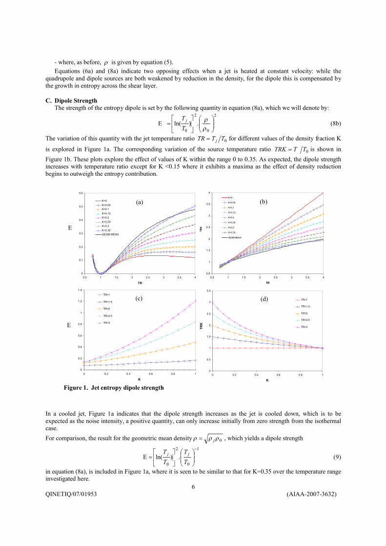
The variation of this quantity with the jet temperature ratio 0TTTR j= for different values of the density fraction K

is explored in Figure 1a. The corresponding variation of the source temperature ratio 0TTTRK = is shown in Figure 1b. These plots explore the effect of values of K within the range 0 to 0.35. As expected, the dipole strength increases with temperature ratio except for K <0.15 where it exhibits a maxima as the effect of density reduction begins to outweigh the entropy contribution.

In a cooled jet, Figure 1a indicates that the dipole strength increases as the jet is cooled down, which is to be expected as the noise intensity, a positive quantity, can only increase initially from zero strength from the isothermal case.For comparison, the result for the geometric mean density 0ρρρ j= , which yields a dipole strength

1

0

2

0.)ln(

−

=Ε

TT

TT jj (9)

in equation (8a), is included in Figure 1a, where it is seen to be similar to that for K=0.35 over the temperature range investigated here.

0.5

1

1.5

2

2.5

3

3.5

4

0.5 1 1.5 2 2.5 3 3.5 4

TR

TRK

K=0

K=0.05

K=0.1

K=0.15

K=0.2

K=0.25

K=0.3

K=0.35

GEOM MEAN

0

0.1

0.2

0.3

0.4

0.5

0.6

0.5 1 1.5 2 2.5 3 3.5 4

TR

E

K=0K=0.05K=0.1K=0.15K=0.2K=0.25K=0.3K=0.35GEOM MEAN

0

0.2

0.4

0.6

0.8

1

1.2

1.4

0 0.2 0.4 0.6 0.8 1

K

E

TR=1

TR=1.5

TR=2

TR=2.5

TR=3

0

0.5

1

1.5

2

2.5

3

3.5

0 0.2 0.4 0.6 0.8 1

K

TRK

TR=1

TR=1.5

TR=2

TR=2.5

TR=3

Figure 1. Jet entropy dipole strength

(a) (b)

(c) (d)

E

E

QINETIQ/07/01953 (AIAA-2007-3632)7

The dependence of the dipole strength on K, over its physically realizable range of 0 to 1, is presented in Figure 1c, for typical jet temperature ratios between 1 and 3. Dipole strength is seen to grow monotonically with K as the reduction in source temperature with increasing K (Figure 1d) reduces the negative effect of density and allows more of the entropy change across the shear layer to contribute to the dipole strength.

D. Overall IntensityIn summary, Lighthill’s theory indicates that for heated jets there are two physical phenomena contributing to the

mixing noise, one arising from momentum transfer across the shear layer and the other from entropy transfer or density inhomogeniety. Both are functions of jet density or temperature but in isothermal jets only momentum transfer is active. By their nature, the two phenomena are effectively interwoven by the turbulent mixing process, but it is unlikely that they are linearly related to any great extent‡ and in the present study we assume that the two source terms in equation (2) are uncorrelated temporally. On this basis, the overall intensity is equal to the sum of the two intensities, namely

222ENRE ppp += (10)

In a related study by Tanner et al38, considerable credence is given to these terms being highly correlated but while this improves their results in some areas it also impairs them in others.

Substituting (6b) and (8b) into equation (10) we obtain, for the overall sound intensity:

8

0

2

0

20

2

0

2

0

20

20

2 ...)ln(..),(.),(..

+=

−−

aV

Dr

TT

aV

DDKDDKpp jjjfdENfqRE ρ

ρθθγ (11)

E. Spectral AnalysisFor this we combine the Strouhal number dependence of the turbulence with dimensional similarity through the

usual integral relationship between overall intensity and power spectral density P ( HzPa /2 ); namely,

∫=max

0

2 .)(f

dffPp (12a)

and njt VSHfP .)()( = (12b)

If mjVp ∝2 then we can readily show in equation (12b) that 1−= mn . In practice we measure jet mixing noise in

1/3rd octave frequency bands for which the level ffPfG .)()( ∝ and it follows that nm = for this case. Thus 1/3rd

octave noise measurements on an isothermal jet should scale as 8jV when plotted against the Strouhal number

jt V

fDS = , whereas the power spectral density scales as 7jV .

Applying similar arguments to equation (6a) we can show that:8

0

2

0

20 ...)(),,(

=

−

aV

Dr

SHfTRVRG jtRERE ρ

ρ ( 2Pa ) (13a)

Likewise, for the entropy noise, equation (8a):6

0

2

0

2

0

20 ..)ln(.).(),,(

=

−

aV

TT

Dr

SHfTRVRG jjtENEN ρ

ρ ( 2Pa ) (13b)

Summing these two equations, the acoustic spectrum at right angles to a heated jet is thus:

8

0

2

0

20

2

0

2

0...)ln(..)()(),,(

+=

−−

aV

Dr

TT

aV

SHSHfTrVRG jjjtENtRE ρ

ρ ( 2Pa ) (14)

‡ Hot-wire measurements31 show, for example, that the third order correlation 2

11 .uu is weak in the shear layer.

QINETIQ/07/01953 (AIAA-2007-3632)8

where REH and ENH are the 1/3rd octave master spectra for the Reynolds and entropy noise respectively.

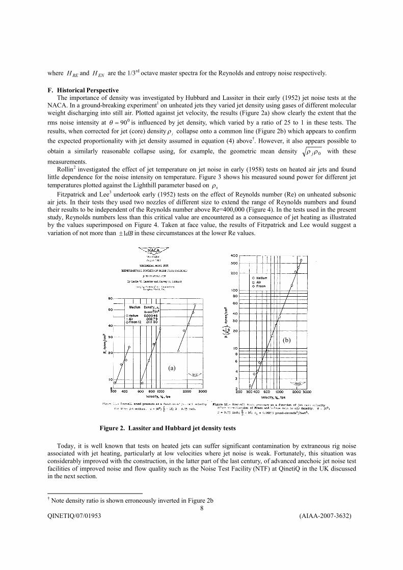
F. Historical Perspective The importance of density was investigated by Hubbard and Lassiter in their early (1952) jet noise tests at the

NACA. In a ground-breaking experiment1 on unheated jets they varied jet density using gases of different molecular weight discharging into still air. Plotted against jet velocity, the results (Figure 2a) show clearly the extent that the rms noise intensity at 090=θ is influenced by jet density, which varied by a ratio of 25 to 1 in these tests. The results, when corrected for jet (core) density jρ collapse onto a common line (Figure 2b) which appears to confirm the expected proportionality with jet density assumed in equation (4) above†. However, it also appears possible to obtain a similarly reasonable collapse using, for example, the geometric mean density 0ρρ j with these measurements.

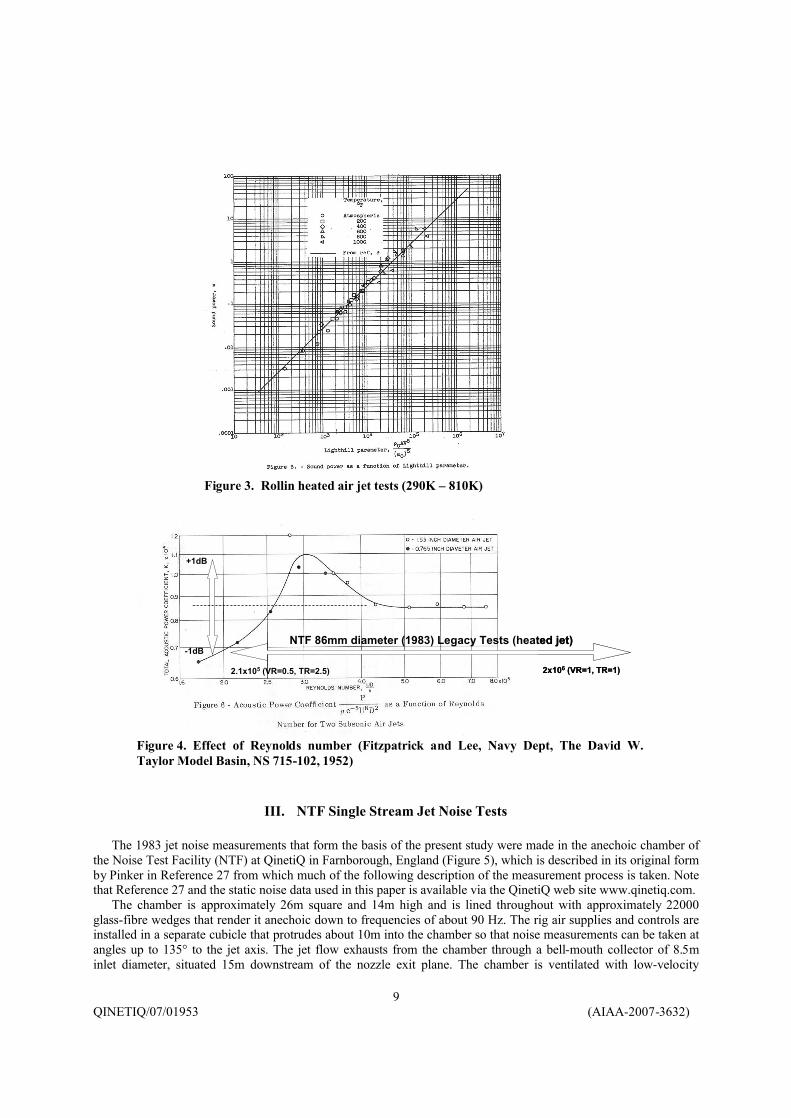
Rollin2 investigated the effect of jet temperature on jet noise in early (1958) tests on heated air jets and found little dependence for the noise intensity on temperature. Figure 3 shows his measured sound power for different jet temperatures plotted against the Lighthill parameter based on 0ρ

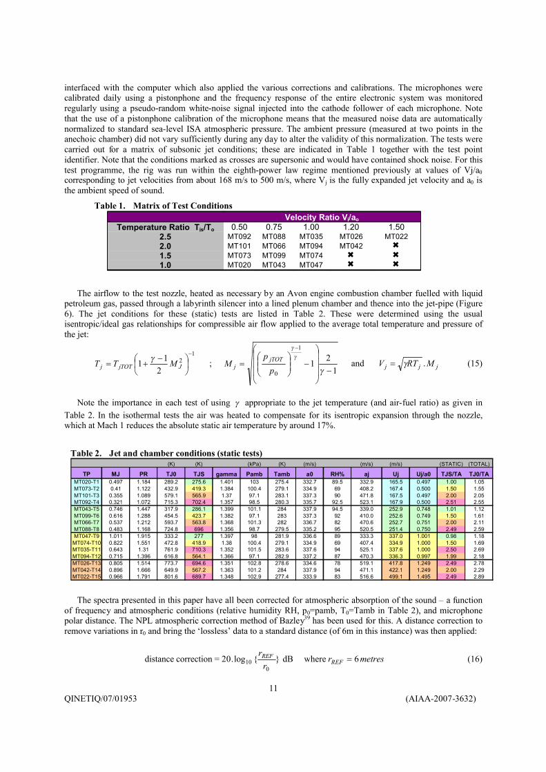
Fitzpatrick and Lee3 undertook early (1952) tests on the effect of Reynolds number (Re) on unheated subsonic air jets. In their tests they used two nozzles of different size to extend the range of Reynolds numbers and found their results to be independent of the Reynolds number above Re=400,000 (Figure 4). In the tests used in the present study, Reynolds numbers less than this critical value are encountered as a consequence of jet heating as illustrated by the values superimposed on Figure 4. Taken at face value, the results of Fitzpatrick and Lee would suggest a variation of not more than dB1± in these circumstances at the lower Re values.

Today, it is well known that tests on heated jets can suffer significant contamination by extraneous rig noise associated with jet heating, particularly at low velocities where jet noise is weak. Fortunately, this situation was considerably improved with the construction, in the latter part of the last century, of advanced anechoic jet noise test facilities of improved noise and flow quality such as the Noise Test Facility (NTF) at QinetiQ in the UK discussed in the next section.

† Note density ratio is shown erroneously inverted in Figure 2b

Figure 2. Lassiter and Hubbard jet density tests

(a)

(b)

QINETIQ/07/01953 (AIAA-2007-3632)9

III. NTF Single Stream Jet Noise Tests

The 1983 jet noise measurements that form the basis of the present study were made in the anechoic chamber of the Noise Test Facility (NTF) at QinetiQ in Farnborough, England (Figure 5), which is described in its original form by Pinker in Reference 27 from which much of the following description of the measurement process is taken. Note that Reference 27 and the static noise data used in this paper is available via the QinetiQ web site www.qinetiq.com.

The chamber is approximately 26m square and 14m high and is lined throughout with approximately 22000 glass-fibre wedges that render it anechoic down to frequencies of about 90 Hz. The rig air supplies and controls are installed in a separate cubicle that protrudes about 10m into the chamber so that noise measurements can be taken at angles up to 135° to the jet axis. The jet flow exhausts from the chamber through a bell-mouth collector of 8.5m inlet diameter, situated 15m downstream of the nozzle exit plane. The chamber is ventilated with low-velocity

Figure 3. Rollin heated air jet tests (290K – 810K)

2.1x105 (VR=0.5, TR=2.5) 2x106 (VR=1, TR=1)

+1dB

-1dBNTF 86mm diameter (1983) Legacy Tests (heated jet)

2.1x105 (VR=0.5, TR=2.5) 2x106 (VR=1, TR=1)

+1dB

-1dBNTF 86mm diameter (1983) Legacy Tests (heated jet)

Figure 4. Effect of Reynolds number (Fitzpatrick and Lee, Navy Dept, The David W. Taylor Model Basin, NS 715-102, 1952)

QINETIQ/07/01953 (AIAA-2007-3632)10

ambient air drawn in through acoustically-lined splitters on each side of the rig cubicle by means of large-capacity fans drawing the air from the downstream end of the exhaust collector through tortuous lined passages.

The test nozzle was 86mm in exit diameter and consisted of a conical taper of 30°, included angle, attached to a 115mm diameter jet-pipe (see Figure 6), giving an area ratio of around 1.8, similar to that of a jet engine. The airflow to the test nozzle, heated as required by an Avon engine combustion chamber fuelled with liquid petroleum gas (LPG), passed through a labyrinth silencer into a lined plenum chamber and thence into the jet-pipe. Note that as well as avoiding wet starts, LPG ensures a gamma value closer to that of Kerosene than is possible with hydrogen orelectric heaters. The 540mm diameter flight stream nozzle (Figure 6) permitted forward flight simulation at velocities up to around 100m/s in the tests.

The noise measurements were taken over a frequency range from 100Hz to 40kHz using ½ inch Bruel and Kjaer microphones positioned at 10° intervals from 30° to 120° to the jet axis, and at polar distances varying from 10.7m to 13.3m from the nozzle. An on-line computer controlled the acquisition and processing of both the acoustic and the aerodynamic data. The acoustic data were analysed by a General Radio third-octave analyser (type 1921)

86mm diameternozzle

Jet-pipe

Flight stream

Flight-streamnozzle, 540mmdiameter

558mmprotrusion

Figure 6. Section through test nozzle

Figure 5. The QinetiQ Noise Test Facility (c1983)

Flight stream nozzle

Far-field microphone masts, r0~12m

86mm test nozzle

QINETIQ/07/01953 (AIAA-2007-3632)11

interfaced with the computer which also applied the various corrections and calibrations. The microphones were calibrated daily using a pistonphone and the frequency response of the entire electronic system was monitored regularly using a pseudo-random white-noise signal injected into the cathode follower of each microphone. Note that the use of a pistonphone calibration of the microphone means that the measured noise data are automatically normalized to standard sea-level ISA atmospheric pressure. The ambient pressure (measured at two points in the anechoic chamber) did not vary sufficiently during any day to alter the validity of this normalization. The tests were carried out for a matrix of subsonic jet conditions; these are indicated in Table 1 together with the test point identifier. Note that the conditions marked as crosses are supersonic and would have contained shock noise. For this test programme, the rig was run within the eighth-power law regime mentioned previously at values of Vj/a0corresponding to jet velocities from about 168 m/s to 500 m/s, where Vj is the fully expanded jet velocity and a0 is the ambient speed of sound.

The airflow to the test nozzle, heated as necessary by an Avon engine combustion chamber fuelled with liquid petroleum gas, passed through a labyrinth silencer into a lined plenum chamber and thence into the jet-pipe (Figure 6). The jet conditions for these (static) tests are listed in Table 2. These were determined using the usual isentropic/ideal gas relationships for compressible air flow applied to the average total temperature and pressure of the jet:

12

211

−

−

+= JjTOTj MTT γ ;1

21

1

0 −

−

=

−

γ

γγ

pp

M jTOTj and jjj MRTV .γ= (15)

Note the importance in each test of using γ appropriate to the jet temperature (and air-fuel ratio) as given in Table 2. In the isothermal tests the air was heated to compensate for its isentropic expansion through the nozzle, which at Mach 1 reduces the absolute static air temperature by around 17%.

The spectra presented in this paper have all been corrected for atmospheric absorption of the sound – a function of frequency and atmospheric conditions (relative humidity RH, p0=pamb, T0=Tamb in Table 2), and microphone polar distance. The NPL atmospheric correction method of Bazley39 has been used for this. A distance correction to remove variations in r0 and bring the ‘lossless’ data to a standard distance (of 6m in this instance) was then applied:

distance correction = }{log.200

10 rrREF dB where metresrREF 6= (16)

Table 2. Jet and chamber conditions (static tests)(K) (K) (kPa) (K) (m/s) (m/s) (m/s) (STATIC) (TOTAL)

TP MJ PR TJ0 TJS gamma Pamb Tamb a0 RH% aj Uj Uj/a0 TJS/TA TJ0/TAMT020-T1 0.497 1.184 289.2 275.6 1.401 103 275.4 332.7 89.5 332.9 165.5 0.497 1.00 1.05MT073-T2 0.41 1.122 432.9 419.3 1.384 100.4 279.1 334.9 69 408.2 167.4 0.500 1.50 1.55MT101-T3 0.355 1.089 579.1 565.9 1.37 97.1 283.1 337.3 90 471.8 167.5 0.497 2.00 2.05MT092-T4 0.321 1.072 715.3 702.4 1.357 98.5 280.3 335.7 92.5 523.1 167.9 0.500 2.51 2.55MT043-T5 0.746 1.447 317.9 286.1 1.399 101.1 284 337.9 94.5 339.0 252.9 0.748 1.01 1.12MT099-T6 0.616 1.288 454.5 423.7 1.382 97.1 283 337.3 92 410.0 252.6 0.749 1.50 1.61MT066-T7 0.537 1.212 593.7 563.8 1.368 101.3 282 336.7 82 470.6 252.7 0.751 2.00 2.11MT088-T8 0.483 1.168 724.8 696 1.356 98.7 279.5 335.2 95 520.5 251.4 0.750 2.49 2.59MT047-T9 1.011 1.915 333.2 277 1.397 98 281.9 336.6 89 333.3 337.0 1.001 0.98 1.18

MT074-T10 0.822 1.551 472.8 418.9 1.38 100.4 279.1 334.9 69 407.4 334.9 1.000 1.50 1.69MT035-T11 0.643 1.31 761.9 710.3 1.352 101.5 283.6 337.6 94 525.1 337.6 1.000 2.50 2.69MT094-T12 0.715 1.396 616.8 564.1 1.366 97.1 282.9 337.2 87 470.3 336.3 0.997 1.99 2.18MT026-T13 0.805 1.514 773.7 694.6 1.351 102.8 278.6 334.6 78 519.1 417.8 1.249 2.49 2.78MT042-T14 0.896 1.666 649.9 567.2 1.363 101.2 284 337.9 94 471.1 422.1 1.249 2.00 2.29MT022-T15 0.966 1.791 801.6 689.7 1.348 102.9 277.4 333.9 83 516.6 499.1 1.495 2.49 2.89

Table 1. Matrix of Test ConditionsVelocity Ratio Vj/ao

Temperature Ratio Tjs/To 0.50 0.75 1.00 1.20 1.502.5 MT092 MT088 MT035 MT026 MT0222.0 MT101 MT066 MT094 MT042 6

1.5 MT073 MT099 MT074 6 6

1.0 MT020 MT043 MT047 6 6

QINETIQ/07/01953 (AIAA-2007-3632)12

IV. Static Data

A. Isothermal JetFigure 7 presents the (lossless) 1/3rd octave spectra measured at right angles to the jet axis for the three

isothermal tests of Table 2; namely, MT020, MT043 and MT047, corresponding to nominal velocity ratios VR=0.5, 0.75 and 1.0 respectively. The high sensitivity to jet velocity of the SPL (~24dB/octave) and the proportional dependence of peak frequency on jet velocity is evident here.

Figure 8 shows the same data normalized on 8VR and plotted against the Strouhal number jVfD / . The good collapse of the data with a peak at 3.1~tS observed here is in agreement with the basic theory, equation (13a), for the isothermal case. The corresponding OASPL for the three isothermal test points is shown in Figure 9 (blue points) where, as expected, they are seen to also follow a 8VR line.

B. Effect of HeatingFigure 9 includes the overall levels for all of the tests of Table 2 and reveals that at the higher velocities, relative

to the isothermal line, the OASPL is reduced by the heating, while at the lower velocities, below about VR=0.7 in these tests, heating increases the OASPL. Compared to the effect of velocity on the OASPL these changes are

65

70

75

80

85

90

95

0.01 0.10 1.00 10.00 100.00St=fD/Uj

SPL

(dB

) -80

.LO

G(V

R)

VR=0.5, TR=1

VR=0.75, TR=1

VR=1, TR=1

Figure 8. SPL normalized on VR8 versus Strouhal number

45

50

55

60

65

70

75

80

85

90

95

100 1000 10000 100000f (Hz)

SPL

(dB

)

VR=0.5, TR=1

VR=0.75, TR=1

VR=1, TR=1

Figure 7. 1/3rd octave SPL at right angleto isothermal jet

70

75

80

85

90

95

100

105

110

115

0.1

OA

SPL

(dB

)

1.0

Vj/a0

V^8

TR=0.85

TR=1.0

TR=1.5

TR=2.0

TR=2.5

0.3 0.5 2.01.0

Figure 9. Overall sound pressure level versus velocity ratio (r0=6m, θ=900)

QINETIQ/07/01953 (AIAA-2007-3632)13

evidently relatively small and it is not difficult to imagine how they might have been overlooked in early tests on jet noise.

The effect of temperature is, however, very noticeable in the noise spectra as revealed in Figure 10, which shows 1/3rd octave noise spectra measured at four temperatures, for both a low and a high jet velocity. For the low velocity test (Figure 10a) progressive increase in SPL below 3000Hz is evident as temperature ratio is increased with little change observed above this frequency. Conversely, for the high velocity case (Figure 10b), the changes occur mostly above 3000Hz except that now the SPL reduces when the temperature is increased. In terms of overall level, the spectra clearly behave in accordance with the OASPL in Figure 9.

In summary, it is evident that temperature has a marked effect on the spectrum of jet mixing noise and that the nature of the effect is a function of jet velocity. It is also evident that no one species or single multi-pole noise component scaling on Strouhal number could be used here to represent the spectrum of a heated jet.

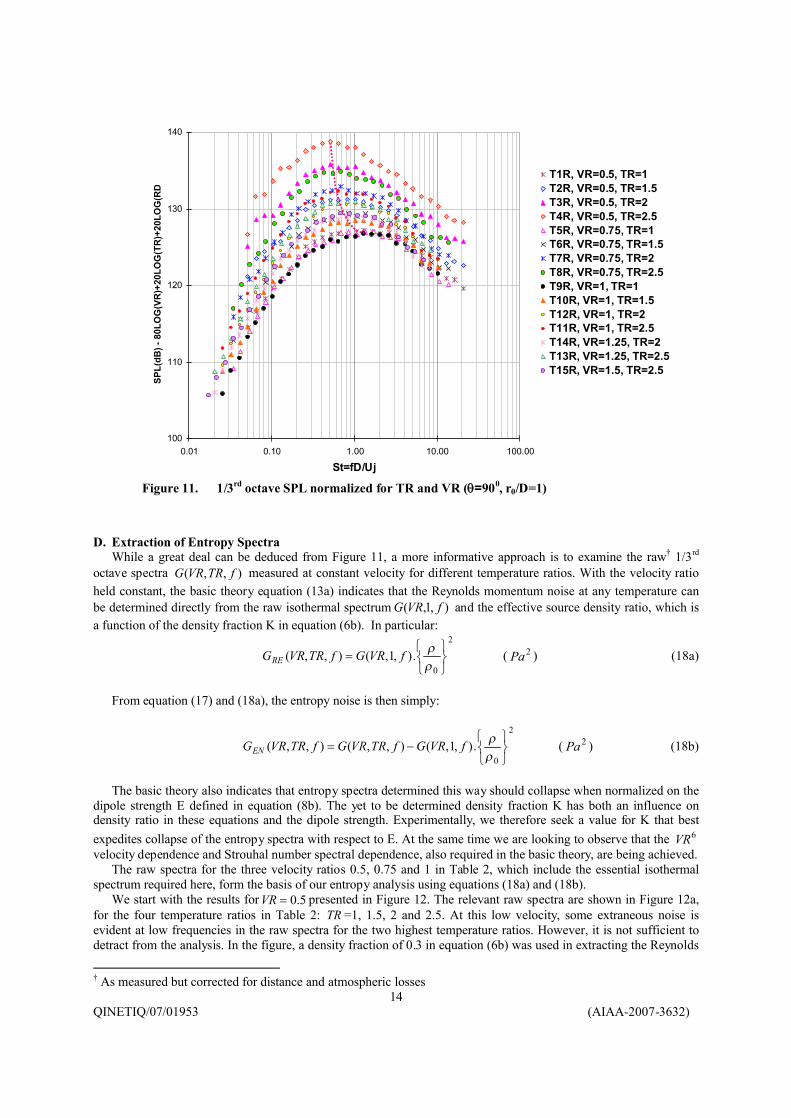
C. Density and Velocity Corrected SpectraFigure 11 presents all of the noise spectra measured at right angles to the jet in the (static) tests of Table 2 plotted

against Strouhal number and normalized for velocity and density. In this instance, the SPLs have been corrected by velocity ratio VR raised to minus eight powers, and by jet temperature ratio TR raised to two powers, corresponding to the use of jet core density in the source region.

A striking feature of these reduced spectra is their relative uniformity given that the measurements were made over a period of time as evident by the different ambient conditions in Table 2. However, this outcome is not fortuitous but rather the result of ensuring that the required temperature and velocity ratios were maintained at all times as can be seen in Table 2, which gives the actual values realized in each test.

In figure 11, the spectra for the isothermal tests ( 1=TR ) are seen to collapse together below the spectra for the heated tests and form a lower envelope to the data ensemble. The heated jet spectra are seen to move progressively upwards as temperature is increased and velocity reduced. At the same time the peak frequency is seen to reduce from a Strouhal number of about 1.3 to 0.5, as indicated by the dotted curve

The fact that none of the hot data appear below the isothermal spectra in Figure 11 is an important observation (note this would not be the case had we used the geometric mean density in the normalization). It encourages us to think of each hot jet spectrum as the sum of two positive components; namely, a momentum noise spectrum and an entropy spectrum, as proposed in Section II; namely,

),,(),,(),,( fTRVRGfTRVRGfTRVRG ENRE += ( 2Pa ) (17)

70

75

80

85

90

95

100 1000 10000 100000f (Hz)

SPL

(dB

)

T9R, VR=1, TR=1

T10R, VR=1, TR=1.5

T12R, VR=1, TR=2

T11R, VR=1, TR=2.5

50

55

60

65

70

75

100 1000 10000 100000f (Hz)

SPL

(dB

)

T1R, VR=0.5, TR=1

T2R, VR=0.5, TR=1.5

T3R, VR=0.5, TR=2

T4R VR=0.5, TR=2.5

Figure 10. Effect of temperature on the noise spectrum for two jet velocities (θ=900)

(a) 168m/s (b) 336m/s

QINETIQ/07/01953 (AIAA-2007-3632)14

D. Extraction of Entropy SpectraWhile a great deal can be deduced from Figure 11, a more informative approach is to examine the raw† 1/3rd

octave spectra ),,( fTRVRG measured at constant velocity for different temperature ratios. With the velocity ratio held constant, the basic theory equation (13a) indicates that the Reynolds momentum noise at any temperature can be determined directly from the raw isothermal spectrum ),1,( fVRG and the effective source density ratio, which is a function of the density fraction K in equation (6b). In particular:

2

0.),1,(),,(

=ρρfVRGfTRVRGRE ( 2Pa ) (18a)

From equation (17) and (18a), the entropy noise is then simply:

2

0.),1,(),,(),,(

−=ρρfVRGfTRVRGfTRVRGEN ( 2Pa ) (18b)

The basic theory also indicates that entropy spectra determined this way should collapse when normalized on the dipole strength E defined in equation (8b). The yet to be determined density fraction K has both an influence on density ratio in these equations and the dipole strength. Experimentally, we therefore seek a value for K that best expedites collapse of the entropy spectra with respect to E. At the same time we are looking to observe that the 6VRvelocity dependence and Strouhal number spectral dependence, also required in the basic theory, are being achieved.

The raw spectra for the three velocity ratios 0.5, 0.75 and 1 in Table 2, which include the essential isothermal spectrum required here, form the basis of our entropy analysis using equations (18a) and (18b).

We start with the results for 5.0=VR presented in Figure 12. The relevant raw spectra are shown in Figure 12a, for the four temperature ratios in Table 2: TR =1, 1.5, 2 and 2.5. At this low velocity, some extraneous noise is evident at low frequencies in the raw spectra for the two highest temperature ratios. However, it is not sufficient to detract from the analysis. In the figure, a density fraction of 0.3 in equation (6b) was used in extracting the Reynolds

† As measured but corrected for distance and atmospheric losses

100

110

120

130

140

0.01 0.10 1.00 10.00 100.00

St=fD/Uj

SPL(

dB) -

80L

OG

(VR

)+20

LOG

(TR

)+20

LOG

(RD

)

T1R, VR=0.5, TR=1T2R, VR=0.5, TR=1.5T3R, VR=0.5, TR=2T4R, VR=0.5, TR=2.5T5R, VR=0.75, TR=1T6R, VR=0.75, TR=1.5T7R, VR=0.75, TR=2T8R, VR=0.75, TR=2.5T9R, VR=1, TR=1T10R, VR=1, TR=1.5T12R, VR=1, TR=2T11R, VR=1, TR=2.5T14R, VR=1.25, TR=2T13R, VR=1.25, TR=2.5T15R, VR=1.5, TR=2.5

Figure 11. 1/3rd octave SPL normalized for TR and VR (θ=900, r0/D=1)

QINETIQ/07/01953 (AIAA-2007-3632)15

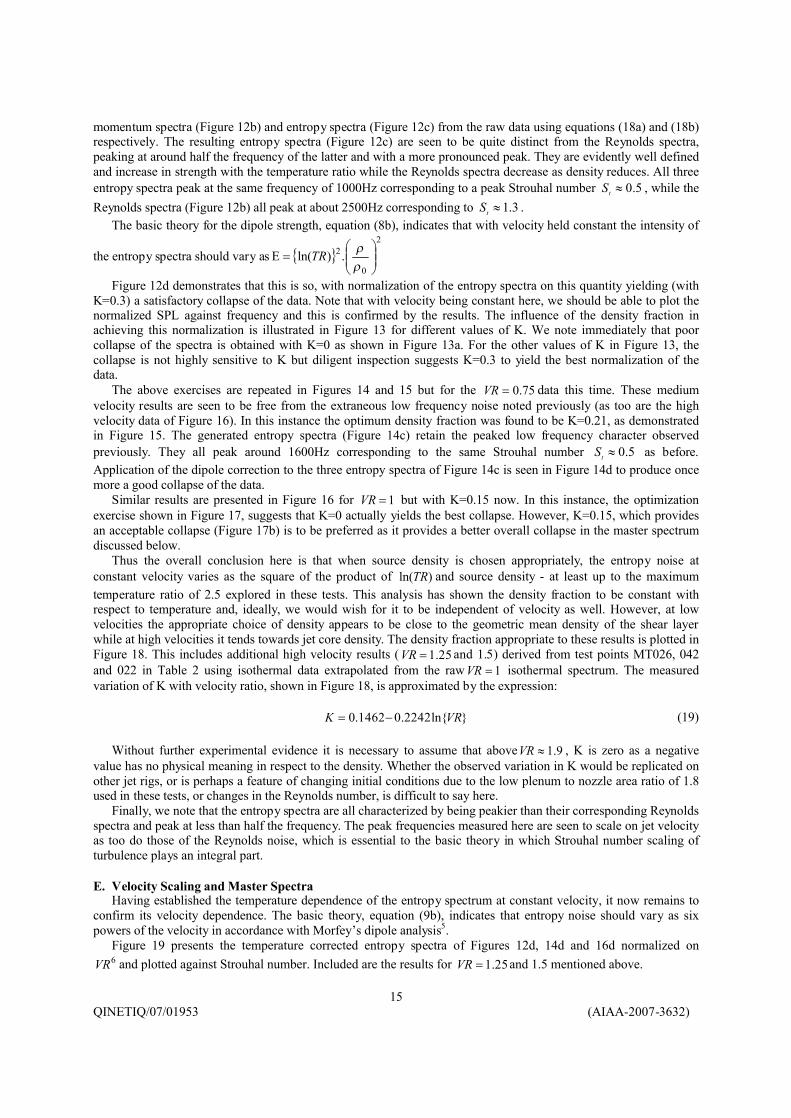
momentum spectra (Figure 12b) and entropy spectra (Figure 12c) from the raw data using equations (18a) and (18b) respectively. The resulting entropy spectra (Figure 12c) are seen to be quite distinct from the Reynolds spectra, peaking at around half the frequency of the latter and with a more pronounced peak. They are evidently well defined and increase in strength with the temperature ratio while the Reynolds spectra decrease as density reduces. All three entropy spectra peak at the same frequency of 1000Hz corresponding to a peak Strouhal number 5.0≈tS , while the Reynolds spectra (Figure 12b) all peak at about 2500Hz corresponding to 3.1≈tS .

The basic theory for the dipole strength, equation (8b), indicates that with velocity held constant the intensity of

the entropy spectra should vary as { }2

0

2 .)ln(

=Ε

ρρTR

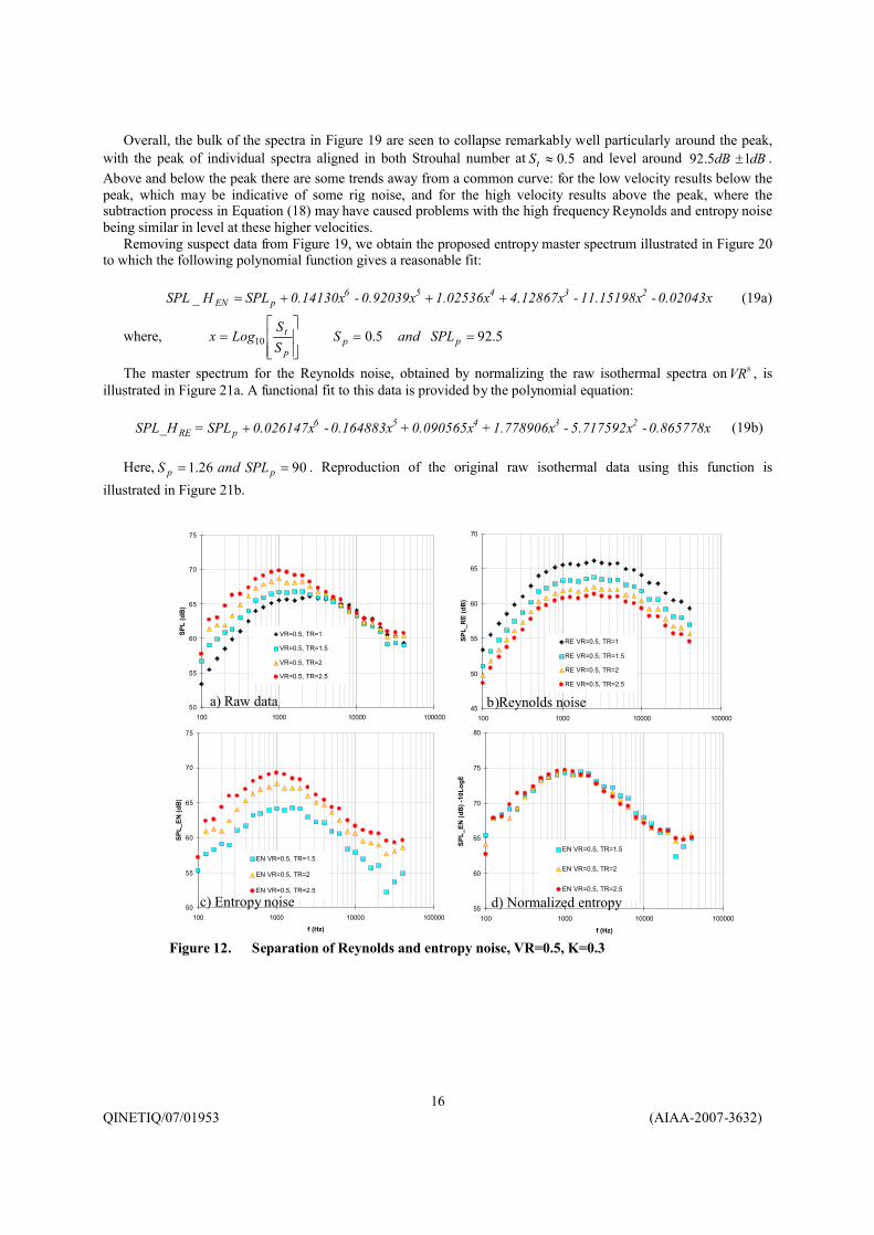
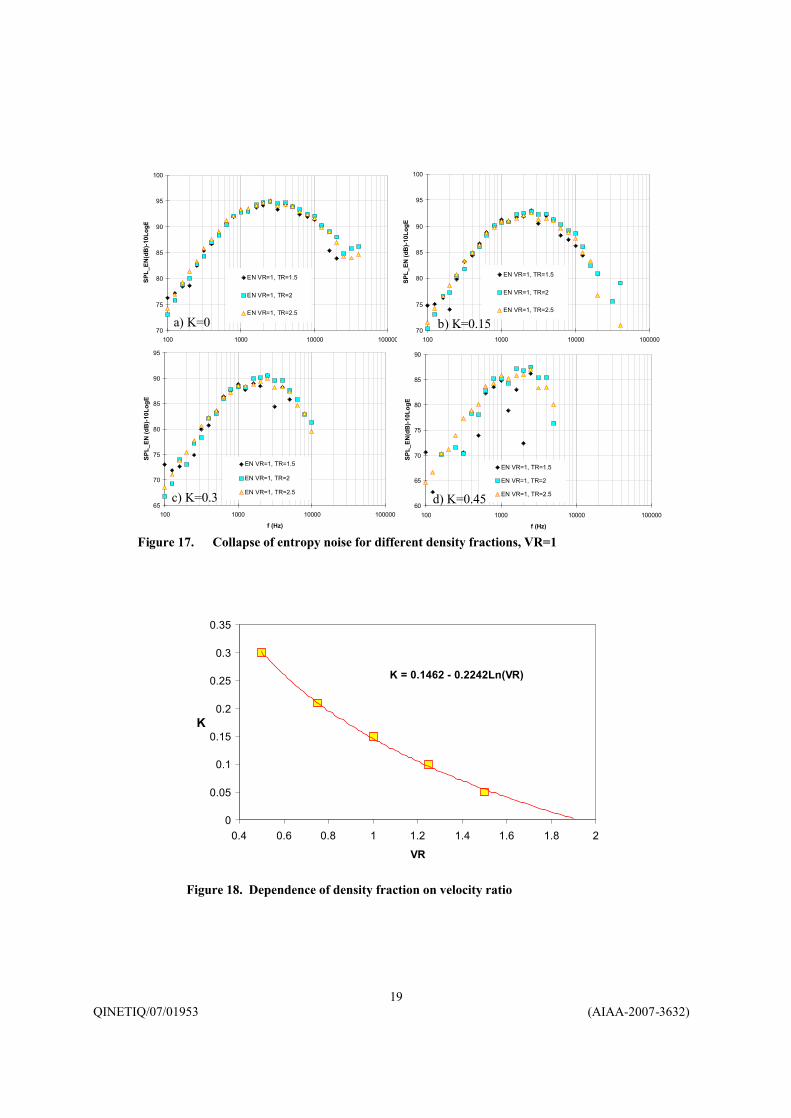
Figure 12d demonstrates that this is so, with normalization of the entropy spectra on this quantity yielding (with K=0.3) a satisfactory collapse of the data. Note that with velocity being constant here, we should be able to plot the normalized SPL against frequency and this is confirmed by the results. The influence of the density fraction in achieving this normalization is illustrated in Figure 13 for different values of K. We note immediately that poor collapse of the spectra is obtained with K=0 as shown in Figure 13a. For the other values of K in Figure 13, the collapse is not highly sensitive to K but diligent inspection suggests K=0.3 to yield the best normalization of the data.

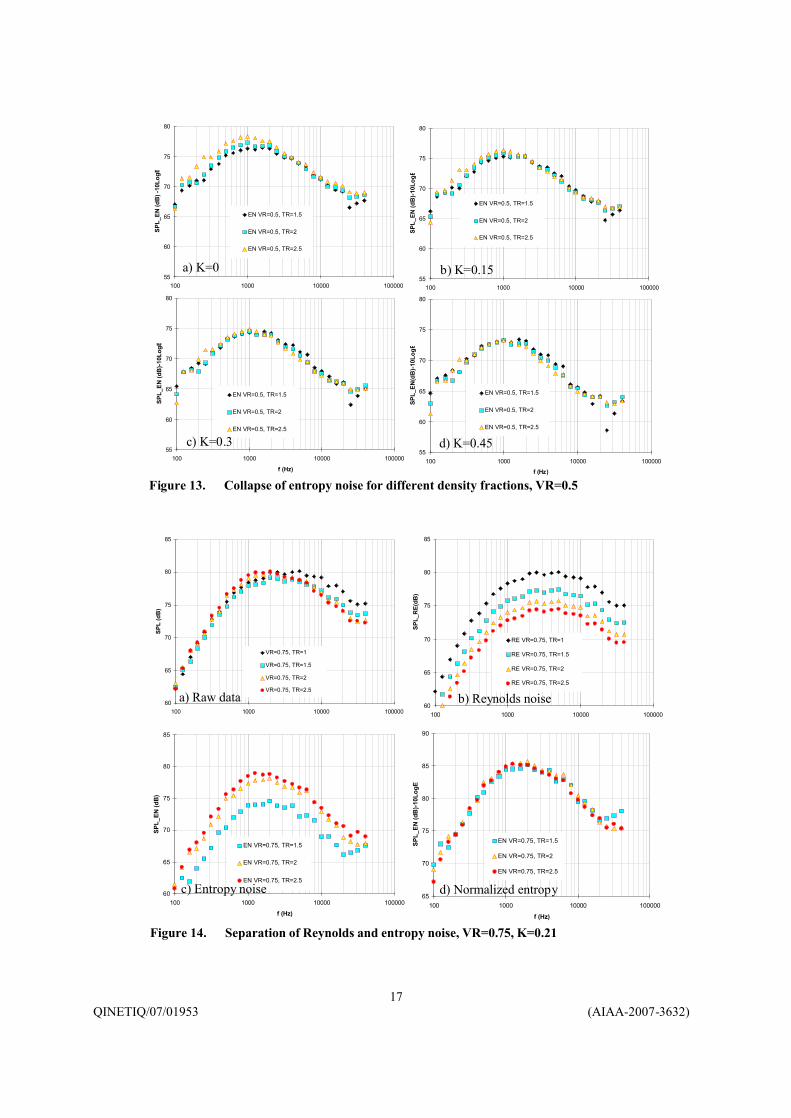
The above exercises are repeated in Figures 14 and 15 but for the 75.0=VR data this time. These medium velocity results are seen to be free from the extraneous low frequency noise noted previously (as too are the high velocity data of Figure 16). In this instance the optimum density fraction was found to be K=0.21, as demonstrated in Figure 15. The generated entropy spectra (Figure 14c) retain the peaked low frequency character observed previously. They all peak around 1600Hz corresponding to the same Strouhal number 5.0≈tS as before. Application of the dipole correction to the three entropy spectra of Figure 14c is seen in Figure 14d to produce once more a good collapse of the data.

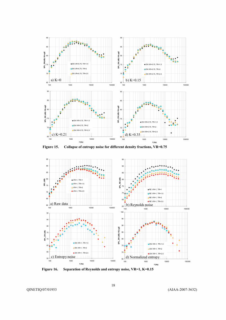
Similar results are presented in Figure 16 for 1=VR but with K=0.15 now. In this instance, the optimizationexercise shown in Figure 17, suggests that K=0 actually yields the best collapse. However, K=0.15, which provides an acceptable collapse (Figure 17b) is to be preferred as it provides a better overall collapse in the master spectrum discussed below.

Thus the overall conclusion here is that when source density is chosen appropriately, the entropy noise at constant velocity varies as the square of the product of )ln(TR and source density - at least up to the maximum temperature ratio of 2.5 explored in these tests. This analysis has shown the density fraction to be constant with respect to temperature and, ideally, we would wish for it to be independent of velocity as well. However, at low velocities the appropriate choice of density appears to be close to the geometric mean density of the shear layer while at high velocities it tends towards jet core density. The density fraction appropriate to these results is plotted in Figure 18. This includes additional high velocity results ( 25.1=VR and 1.5) derived from test points MT026, 042 and 022 in Table 2 using isothermal data extrapolated from the raw 1=VR isothermal spectrum. The measured variation of K with velocity ratio, shown in Figure 18, is approximated by the expression:

}ln{2242.01462.0 VRK −= (19)

Without further experimental evidence it is necessary to assume that above 9.1≈VR , K is zero as a negative value has no physical meaning in respect to the density. Whether the observed variation in K would be replicated on other jet rigs, or is perhaps a feature of changing initial conditions due to the low plenum to nozzle area ratio of 1.8 used in these tests, or changes in the Reynolds number, is difficult to say here.

Finally, we note that the entropy spectra are all characterized by being peakier than their corresponding Reynolds spectra and peak at less than half the frequency. The peak frequencies measured here are seen to scale on jet velocity as too do those of the Reynolds noise, which is essential to the basic theory in which Strouhal number scaling of turbulence plays an integral part.

E. Velocity Scaling and Master SpectraHaving established the temperature dependence of the entropy spectrum at constant velocity, it now remains to

confirm its velocity dependence. The basic theory, equation (9b), indicates that entropy noise should vary as six powers of the velocity in accordance with Morfey’s dipole analysis5.

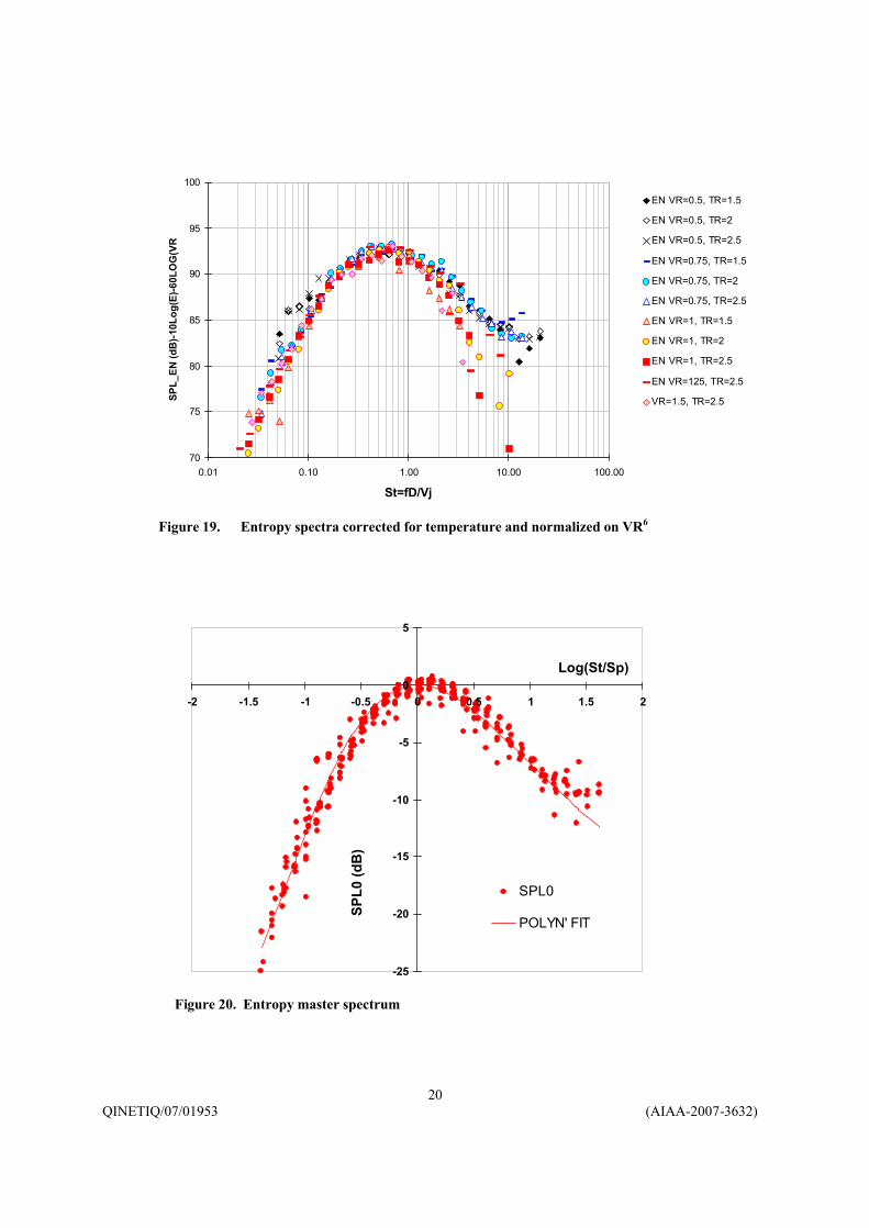
Figure 19 presents the temperature corrected entropy spectra of Figures 12d, 14d and 16d normalized on 6VR and plotted against Strouhal number. Included are the results for 25.1=VR and 1.5 mentioned above.

QINETIQ/07/01953 (AIAA-2007-3632)16

Overall, the bulk of the spectra in Figure 19 are seen to collapse remarkably well particularly around the peak, with the peak of individual spectra aligned in both Strouhal number at 5.0≈tS and level around dB5.92 dB1± . Above and below the peak there are some trends away from a common curve: for the low velocity results below the peak, which may be indicative of some rig noise, and for the high velocity results above the peak, where the subtraction process in Equation (18) may have caused problems with the high frequency Reynolds and entropy noise being similar in level at these higher velocities.

Removing suspect data from Figure 19, we obtain the proposed entropy master spectrum illustrated in Figure 20 to which the following polynomial function gives a reasonable fit:

0.02043x-11.15198x-4.12867x1.02536x0.92039x-0.14130xSPLHSPL 23456pEN +++=_ (19a)

where,

=

p

t

SS

Logx 10 5.925.0 == pp SPLandS

The master spectrum for the Reynolds noise, obtained by normalizing the raw isothermal spectra on 8VR , is illustrated in Figure 21a. A functional fit to this data is provided by the polynomial equation:

0.865778x-5.717592x-1.778906x+0.090565x+0.164883x-0.026147xSPL=SPL_H 23456pRE + (19b)

Here, 9026.1 == pp SPLandS . Reproduction of the original raw isothermal data using this function is illustrated in Figure 21b.

50

55

60

65

70

75

100 1000 10000 100000

f (Hz)

SPL

(dB

)

VR=0.5, TR=1

VR=0.5, TR=1.5

VR=0.5, TR=2

VR=0.5, TR=2.5

45

50

55

60

65

70

100 1000 10000 100000

f (Hz)

SPL_

RE

(dB

)

RE VR=0.5, TR=1

RE VR=0.5, TR=1.5

RE VR=0.5, TR=2

RE VR=0.5, TR=2.5

50

55

60

65

70

75

100 1000 10000 100000

f (Hz)

SPL_

EN (d

B)

EN VR=0.5, TR=1.5

EN VR=0.5, TR=2

EN VR=0.5, TR=2.5

55

60

65

70

75

80

100 1000 10000 100000

f (Hz)

SPL_

EN (d

B) -

10Lo

gE

EN VR=0.5, TR=1.5

EN VR=0.5, TR=2

EN VR=0.5, TR=2.5

Figure 12. Separation of Reynolds and entropy noise, VR=0.5, K=0.3

a) Raw data b)Reynolds noise

c) Entropy noise d) Normalized entropy

QINETIQ/07/01953 (AIAA-2007-3632)17

60

65

70

75

80

85

100 1000 10000 100000

SPL

(dB

)

VR=0.75, TR=1

VR=0.75, TR=1.5

VR=0.75, TR=2

VR=0.75, TR=2.5

60

65

70

75

80

85

100 1000 10000 100000

SPL_

RE(

dB)

RE VR=0.75, TR=1

RE VR=0.75, TR=1.5

RE VR=0.75, TR=2

RE VR=0.75, TR=2.5

60

65

70

75

80

85

100 1000 10000 100000

f (Hz)

SPL_

EN (d

B)

EN VR=0.75, TR=1.5

EN VR=0.75, TR=2

EN VR=0.75, TR=2.5

65

70

75

80

85

90

100 1000 10000 100000

f (Hz)

SPL_

EN (d

B)-1

0Log

E

EN VR=0.75, TR=1.5

EN VR=0.75, TR=2

EN VR=0.75, TR=2.5

Figure 14. Separation of Reynolds and entropy noise, VR=0.75, K=0.21

a) Raw data b) Reynolds noise

c) Entropy noise d) Normalized entropy

55

60

65

70

75

80

100 1000 10000 100000

SPL_

EN (d

B) -

10Lo

gE

EN VR=0.5, TR=1.5

EN VR=0.5, TR=2

EN VR=0.5, TR=2.5

55

60

65

70

75

80

100 1000 10000 100000

SPL_

EN (d

B)-1

0Log

E

EN VR=0.5, TR=1.5

EN VR=0.5, TR=2

EN VR=0.5, TR=2.5

55

60

65

70

75

80

100 1000 10000 100000

f (Hz)

SPL_

EN (d

B)-1

0Log

E

EN VR=0.5, TR=1.5

EN VR=0.5, TR=2

EN VR=0.5, TR=2.5

55

60

65

70

75

80

100 1000 10000 100000

f (Hz)

SPL_

EN(d

B)-1

0Log

E

EN VR=0.5, TR=1.5

EN VR=0.5, TR=2

EN VR=0.5, TR=2.5

Figure 13. Collapse of entropy noise for different density fractions, VR=0.5

a) K=0 b) K=0.15

c) K=0.3 d) K=0.45

QINETIQ/07/01953 (AIAA-2007-3632)18

60

65

70

75

80

85

90

95

100 1000 10000 100000

SPL_

RE

(dB

)

RE VR=1, TR=1

RE VR=1, TR=1.5

RE VR=1, TR=2

RE VR=1, TR=2.5

55

60

65

70

75

80

85

90

100 1000 10000 100000

f (Hz)

SPL_

EN (d

B)

EN VR=1, TR=1.5

EN VR=1, TR=2

EN VR=1, TR=2.5

65

70

75

80

85

90

95

100

100 1000 10000 100000

f (Hz)

SPL_

EN (d

B)-1

0Log

E

EN VR=1, TR=1.5

EN VR=1, TR=2

EN VR=1, TR=2.5

60

65

70

75

80

85

90

95

100 1000 10000 100000

f (Hz)

SPL

(dB

)

VR=1, TR=1

VR=1, TR=1.5

VR=1, TR=2

VR=1, TR=2.5

Figure 16. Separation of Reynolds and entropy noise, VR=1, K=0.15

c) Entropy noise d) Normalized entropy

a) Raw data b) Reynolds noise

65

70

75

80

85

90

100 1000 10000 100000

f (Hz)

SPL_

EN(d

B)-1

0Log

E

EN VR=0.75, TR=1.5

EN VR=0.75, TR=2

EN VR=0.75, TR=2.5

65

70

75

80

85

90

100 1000 10000 100000

SPL_

EN (d

B)-1

0Log

E

EN VR=0.75, TR=1.5

EN VR=0.75, TR=2

EN VR=0.75, TR=2.5

65

70

75

80

85

90

100 1000 10000 100000

f (Hz)

SPL_

EN (d

B)-1

0Log

E

EN VR=0.75, TR=1.5

EN VR=0.75, TR=2

EN VR=0.75, TR=2.5

65

70

75

80

85

90

100 1000 10000 100000

f (Hz)

SPL_

EN (d

B)-1

0Log

E

EN VR=0.75, TR=1.5

EN VR=0.75, TR=2

EN VR=0.75, TR=2.5

Figure 15. Collapse of entropy noise for different density fractions, VR=0.75

a) K=0 b) K=0.15

c) K=0.21 d) K=0.35

QINETIQ/07/01953 (AIAA-2007-3632)19

K = 0.1462 - 0.2242Ln(VR)

0

0.05

0.1

0.15

0.2

0.25

0.3

0.35

0.4 0.6 0.8 1 1.2 1.4 1.6 1.8 2

VR

K

Figure 18. Dependence of density fraction on velocity ratio

70

75

80

85

90

95

100

100 1000 10000 100000

SPL_

EN(d

B)-1

0Log

E

EN VR=1, TR=1.5

EN VR=1, TR=2

EN VR=1, TR=2.5

70

75

80

85

90

95

100

100 1000 10000 100000

SPL_

EN (d

B)-1

0Log

E

EN VR=1, TR=1.5

EN VR=1, TR=2

EN VR=1, TR=2.5

65

70

75

80

85

90

95

100 1000 10000 100000

f (Hz)

SPL_

EN (d

B)-1

0Log

E

EN VR=1, TR=1.5

EN VR=1, TR=2

EN VR=1, TR=2.5

60

65

70

75

80

85

90

100 1000 10000 100000

f (Hz)

SPL_

EN(d

B)-1

0Log

E

EN VR=1, TR=1.5

EN VR=1, TR=2

EN VR=1, TR=2.5

Figure 17. Collapse of entropy noise for different density fractions, VR=1

c) K=0.3 d) K=0.45

a) K=0 b) K=0.15

QINETIQ/07/01953 (AIAA-2007-3632)20

70

75

80

85

90

95

100

0.01 0.10 1.00 10.00 100.00

St=fD/Vj

SPL_

EN (d

B)-1

0Log

(E)-6

0LO

G(V

R)

EN VR=0.5, TR=1.5

EN VR=0.5, TR=2

EN VR=0.5, TR=2.5

EN VR=0.75, TR=1.5

EN VR=0.75, TR=2

EN VR=0.75, TR=2.5

EN VR=1, TR=1.5

EN VR=1, TR=2

EN VR=1, TR=2.5

EN VR=125, TR=2.5

VR=1.5, TR=2.5

Figure 19. Entropy spectra corrected for temperature and normalized on VR6

-25

-20

-15

-10

-5

0

5

-2 -1.5 -1 -0.5 0 0.5 1 1.5 2

Log(St/Sp)

SPL0

(dB

)

SPL0

POLYN' FIT

Figure 20. Entropy master spectrum

QINETIQ/07/01953 (AIAA-2007-3632)21

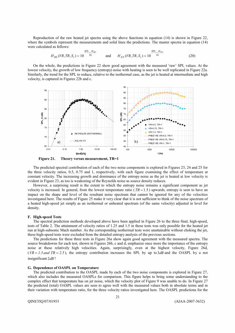
Reproduction of the raw heated jet spectra using the above functions in equation (14) is shown in Figure 22, where the symbols represent the measurements and solid lines the predictions. The master spectra in equation (14) were calculated as follows:

10_

10),,(REHSPL

tRE STRVRH = and 10_

10),,(ENHSPL

tEN STRVRH = (20)

On the whole, the predictions in Figure 22 show good agreement with the measured ‘raw’ SPL values. At the lowest velocity, the growth of low frequency (entropy) noise with heating is seen to be well replicated in Figure 22a. Similarly, the trend for the SPL to reduce, relative to the isothermal case, as the jet is heated at intermediate and high velocity, is captured in Figures 22b and c.

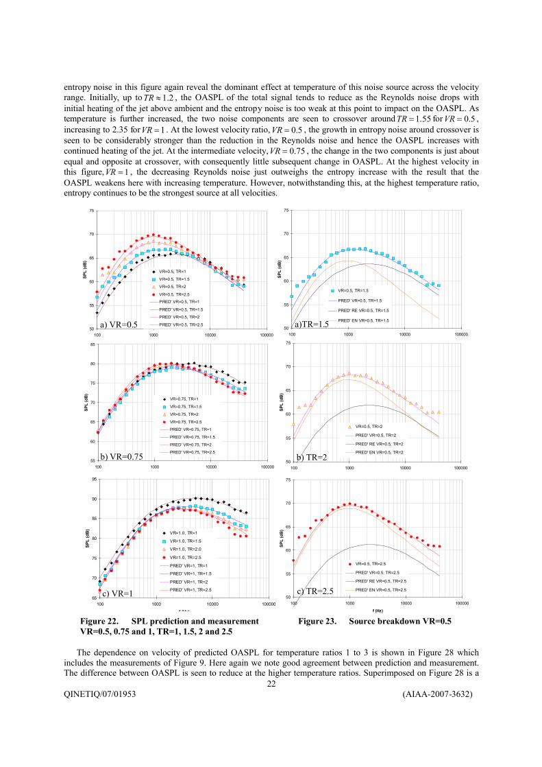
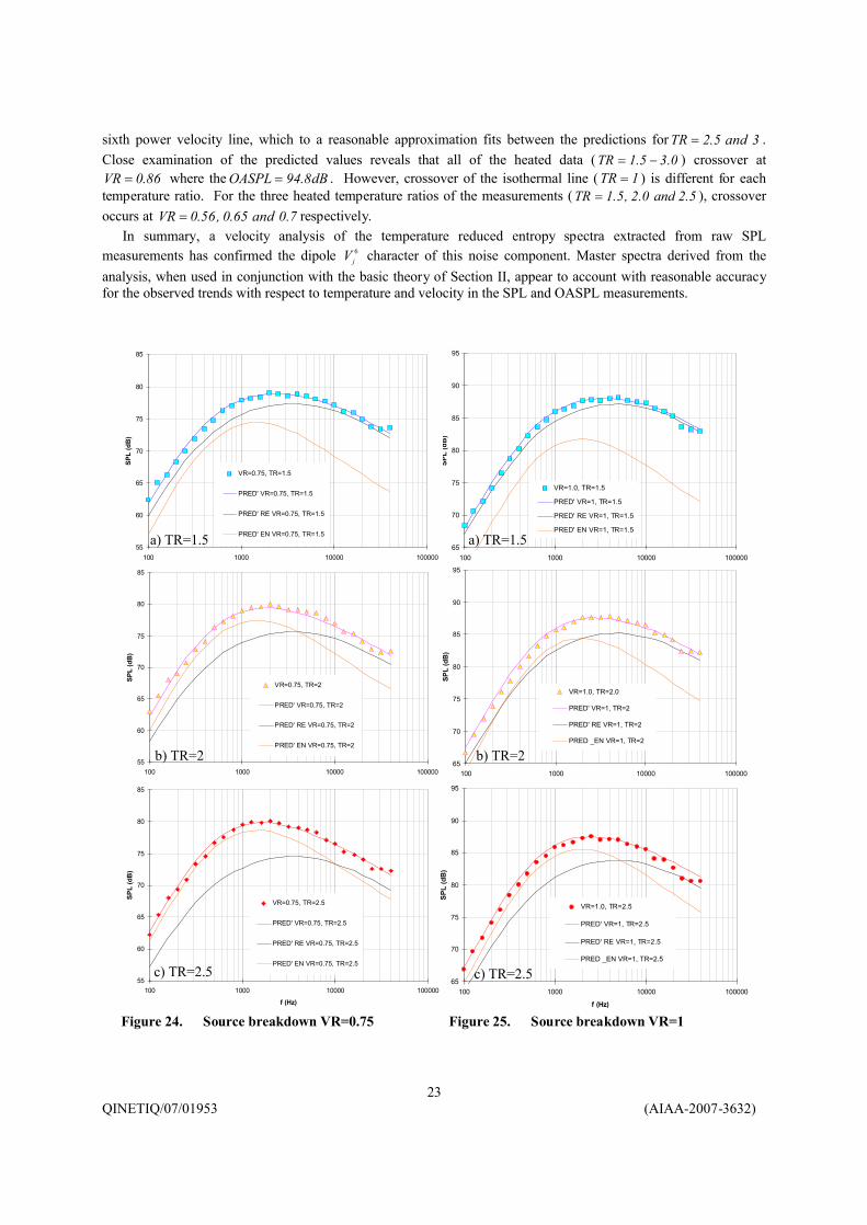
The predicted spectral contribution of each of the two noise components is explored in Figures 23, 24 and 25 for the three velocity ratios, 0.5, 0.75 and 1, respectively, with each figure examining the effect of temperature at constant velocity. The increasing growth and dominance of the entropy noise as the jet is heated at low velocity is evident in Figure 23, as too is weakening of the Reynolds noise as source density reduces.

However, a surprising result is the extent to which the entropy noise remains a significant component as jet velocity is increased. In general, from the lowest temperature ratio ( 5.1=TR ) upwards, entropy is seen to have an impact on the shape and level of the resultant noise spectrum that cannot be ignored for any of the velocities investigated here. The results of Figure 25 make it very clear that it is not sufficient to think of the noise spectrum of a heated high-speed jet simply as an isothermal or unheated spectrum (of the same velocity) adjusted in level for density.

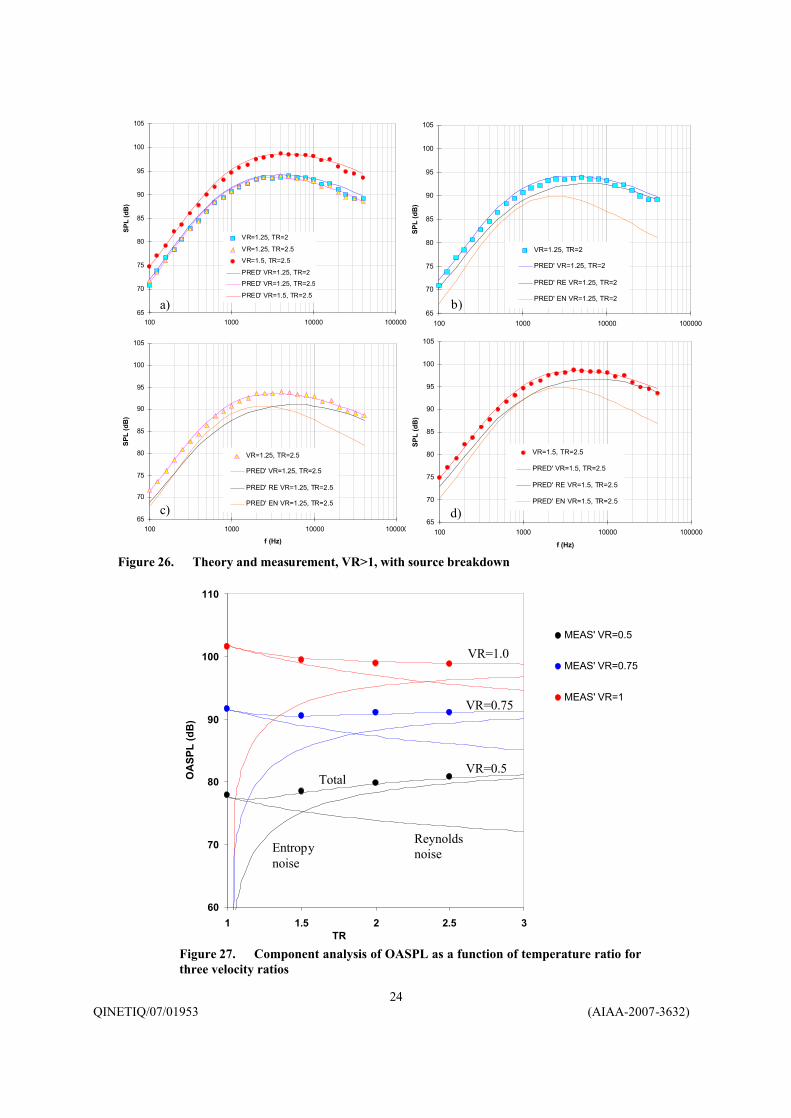
F. High-speed TestsThe spectral prediction methods developed above have been applied in Figure 26 to the three final, high-speed,

tests of Table 2. The attainment of velocity ratios of 1.25 and 1.5 in these tests was only possible for the heated jet run at high-subsonic Mach number. As the corresponding isothermal tests were unattainable without choking the jet, these high-speed tests were excluded from the detailed entropy analysis of the previous sections.

The predictions for these three tests in Figure 26a show again good agreement with the measured spectra. The source breakdowns for each test, shown in Figures 26b, c and d, emphasize once more the importance of the entropy noise at these relatively high velocities. Again, surprisingly, even at the highest velocity, Figure 26d, ( 5.2TRand5.1VR == ), the entropy contribution increases the SPL by up to dB3 and the OASPL by a not insignificant dB2 !

G. Dependence of OASPL on TemperatureThe predicted contribution to the OASPL made by each of the two noise components is explored in Figure 27,

which also includes the measured OASPLs for comparison. This figure helps to bring some understanding to the complex effect that temperature has on jet noise, which the velocity plot of Figure 9 was unable to do. In Figure 27 the predicted (total) OASPL values are seen to agree well with the measured values both in absolute terms and in their variation with temperature ratio, for the three velocity ratios investigated here. The OASPL predictions for the

40

45

50

55

60

65

70

75

80

85

90

95

100 1000 10000 100000

f (Hz)

SPL

(dB

)VR=0.5, TR=1

VR=0.75, TR=1

VR=1.0, TR=1

PRED' RE VR=0.5, TR=1

PRED' RE VR=0.75, TR=1

PRED' RE VR=1, TR=165

70

75

80

85

90

95

0.01 0.10 1.00 10.00 100.00

St=fD/Vj

SPL_

H (d

B)

REYNOLDS (ISOTHERMAL)

POLYN' FIT

Figure 21. Theory versus measurement, TR=1

a) b)

QINETIQ/07/01953 (AIAA-2007-3632)22

entropy noise in this figure again reveal the dominant effect at temperature of this noise source across the velocity range. Initially, up to 2.1≈TR , the OASPL of the total signal tends to reduce as the Reynolds noise drops with initial heating of the jet above ambient and the entropy noise is too weak at this point to impact on the OASPL. As temperature is further increased, the two noise components are seen to crossover around 55.1=TR for 5.0=VR , increasing to 2.35 for 1=VR . At the lowest velocity ratio, 5.0=VR , the growth in entropy noise around crossover is seen to be considerably stronger than the reduction in the Reynolds noise and hence the OASPL increases with continued heating of the jet. At the intermediate velocity, 75.0=VR , the change in the two components is just about equal and opposite at crossover, with consequently little subsequent change in OASPL. At the highest velocity in this figure, 1=VR , the decreasing Reynolds noise just outweighs the entropy increase with the result that the OASPL weakens here with increasing temperature. However, notwithstanding this, at the highest temperature ratio, entropy continues to be the strongest source at all velocities.

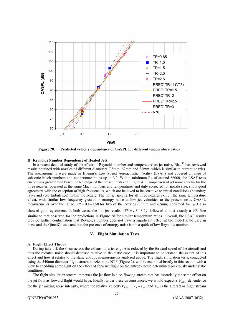
The dependence on velocity of predicted OASPL for temperature ratios 1 to 3 is shown in Figure 28 which includes the measurements of Figure 9. Here again we note good agreement between prediction and measurement. The difference between OASPL is seen to reduce at the higher temperature ratios. Superimposed on Figure 28 is a

65

70

75

80

85

90

95

100 1000 10000 100000

f (Hz)

SPL

(dB

)

VR=1.0, TR=1

VR=1.0, TR=1.5

VR=1.0, TR=2.0

VR=1.0, TR=2.5

PRED' VR=1, TR=1

PRED' VR=1, TR=1.5

PRED' VR=1, TR=2

PRED' VR=1, TR=2.5

55

60

65

70

75

80

85

100 1000 10000 100000

f (Hz)

SPL

(dB

)

VR=0.75, TR=1

VR=0.75, TR=1.5

VR=0.75, TR=2

VR=0.75, TR=2.5

PRED' VR=0.75, TR=1

PRED' VR=0.75, TR=1.5

PRED' VR=0.75, TR=2

PRED' VR=0.75, TR=2.5

50

55

60

65

70

75

100 1000 10000 100000

f (Hz)

SPL

(dB

)

VR=0.5, TR=1

VR=0.5, TR=1.5

VR=0.5, TR=2

VR=0.5, TR=2.5

PRED' VR=0.5, TR=1

PRED' VR=0.5, TR=1.5

PRED' VR=0.5, TR=2

PRED' VR=0.5, TR=2.550

55

60

65

70

75

100 1000 10000 100000

f (Hz)

SPL

(dB

)

VR=0.5, TR=1.5

PRED' VR=0.5, TR=1.5

PRED' RE VR=0.5, TR=1.5

PRED' EN VR=0.5, TR=1.5

50

55

60

65

70

75

100 1000 10000 100000

SPL

(dB

)

VR=0.5, TR=2

PRED' VR=0.5, TR=2

PRED' RE VR=0.5, TR=2

PRED' EN VR=0.5, TR=2

50

55

60

65

70

75

100 1000 10000 100000

f (Hz)

SPL

(dB

)

VR=0.5, TR=2.5

PRED' VR=0.5, TR=2.5

PRED' RE VR=0.5, TR=2.5

PRED' EN VR=0.5, TR=2.5

Figure 22. SPL prediction and measurement Figure 23. Source breakdown VR=0.5VR=0.5, 0.75 and 1, TR=1, 1.5, 2 and 2.5

a) VR=0.5

b) VR=0.75

c) VR=1

a)TR=1.5

b) TR=2

c) TR=2.5

QINETIQ/07/01953 (AIAA-2007-3632)23

sixth power velocity line, which to a reasonable approximation fits between the predictions for 3and5.2TR = . Close examination of the predicted values reveals that all of the heated data ( 0.35.1TR −= ) crossover at

86.0VR = where the dB8.94OASPL = . However, crossover of the isothermal line ( 1TR = ) is different for each temperature ratio. For the three heated temperature ratios of the measurements ( 5.2and0.2,5.1TR = ), crossover occurs at 7.0and65.0,56.0VR = respectively.

In summary, a velocity analysis of the temperature reduced entropy spectra extracted from raw SPL measurements has confirmed the dipole 6

jV character of this noise component. Master spectra derived from the analysis, when used in conjunction with the basic theory of Section II, appear to account with reasonable accuracy for the observed trends with respect to temperature and velocity in the SPL and OASPL measurements.

65

70

75

80

85

90

95

100 1000 10000 100000

f (Hz)

SPL

(dB

)

VR=1.0, TR=1.5

PRED' VR=1, TR=1.5

PRED' RE VR=1, TR=1.5

PRED' EN VR=1, TR=1.5

65

70

75

80

85

90

95

100 1000 10000 100000

f (Hz)

SPL

(dB

)

VR=1.0, TR=2.0

PRED' VR=1, TR=2

PRED' RE VR=1, TR=2

PRED _EN VR=1, TR=2

65

70

75

80

85

90

95

100 1000 10000 100000

f (Hz)

SPL

(dB

)

VR=1.0, TR=2.5

PRED' VR=1, TR=2.5

PRED' RE VR=1, TR=2.5

PRED _EN VR=1, TR=2.5

55

60

65

70

75

80

85

100 1000 10000 100000

f (Hz)

SPL

(dB

)

VR=0.75, TR=1.5

PRED' VR=0.75, TR=1.5

PRED' RE VR=0.75, TR=1.5

PRED' EN VR=0.75, TR=1.5

55

60

65

70

75

80

85

100 1000 10000 100000

SPL

(dB

)

VR=0.75, TR=2

PRED' VR=0.75, TR=2

PRED' RE VR=0.75, TR=2

PRED' EN VR=0.75, TR=2

55

60

65

70

75

80

85

100 1000 10000 100000

f (Hz)

SPL

(dB

)

VR=0.75, TR=2.5

PRED' VR=0.75, TR=2.5

PRED' RE VR=0.75, TR=2.5

PRED' EN VR=0.75, TR=2.5

Figure 24. Source breakdown VR=0.75 Figure 25. Source breakdown VR=1

a) TR=1.5 a) TR=1.5

b) TR=2

c) TR=2.5

b) TR=2

c) TR=2.5

QINETIQ/07/01953 (AIAA-2007-3632)24

60

70

80

90

100

110

1 1.5 2 2.5 3TR

OA

SPL

(dB

)

MEAS' VR=0.5

MEAS' VR=0.75

MEAS' VR=1

Figure 27. Component analysis of OASPL as a function of temperature ratio for three velocity ratios

Entropy noise

Reynolds noise

VR=0.75

VR=1.0

VR=0.5Total

65

70

75

80

85

90

95

100

105

100 1000 10000 100000

SPL

(dB

)

VR=1.25, TR=2

PRED' VR=1.25, TR=2

PRED' RE VR=1.25, TR=2

PRED' EN VR=1.25, TR=2

65

70

75

80

85

90

95

100

105

100 1000 10000 100000

f (Hz)

SPL

(dB

)

VR=1.25, TR=2.5

PRED' VR=1.25, TR=2.5

PRED' RE VR=1.25, TR=2.5

PRED' EN VR=1.25, TR=2.5

65

70

75

80

85

90

95

100

105

100 1000 10000 100000

f (Hz)

SPL

(dB

)

VR=1.5, TR=2.5

PRED' VR=1.5, TR=2.5

PRED' RE VR=1.5, TR=2.5

PRED' EN VR=1.5, TR=2.5

65

70

75

80

85

90

95

100

105

100 1000 10000 100000

SPL

(dB

)

VR=1.25, TR=2

VR=1.25, TR=2.5

VR=1.5, TR=2.5

PRED' VR=1.25, TR=2

PRED' VR=1.25, TR=2.5

PRED' VR=1.5, TR=2.5

Figure 26. Theory and measurement, VR>1, with source breakdown

a) b)

c) d)

QINETIQ/07/01953 (AIAA-2007-3632)25

H. Reynolds Number Dependence of Heated JetsIn a recent detailed study of the effect of Reynolds number and temperature on jet noise, Bhat40 has reviewed

results obtained with nozzles of different diameters (38mm, 62mm and 88mm, which is similar to current nozzle). The measurements were made in Boeing’s Low Speed Aeroacoustic Facility (LSAF) and covered a range of subsonic Mach numbers and temperature ratios up to 3.2. With a minimum Re of around 86000, the LSAF tests encompass greater than twice the Re range of the present tests (c.f. Figure 4). Comparison of jet noise spectra for the three nozzles, operated at the same Mach numbers and temperatures and duly corrected for nozzle size, show good agreement with the exception of high frequencies, which are believed to be sensitive to initial conditions (boundary layer and core turbulence) within the nozzle. The hot jet spectra for all three nozzles exhibit the same temperature effect, with similar low frequency growth in entropy noise at low jet velocities to the present tests. OASPL measurements over the range 58.14.0 −=VR for two of the nozzles (38mm and 62mm) corrected for r0/D also

showed good agreement. In both cases, the hot jet results )2.38.1TR( −= followed almost exactly a 6VR line similar to that observed for the predictions in Figure 28 for similar temperature ratios. Overall, the LSAF results provide further confirmation that Reynolds number does not have a significant effect at the model scale used in these and the QinetiQ tests, and that the presence of entropy noise is not a quirk of low Reynolds number.

V. Flight Simulation Tests

A. Flight Effect TheoryDuring take-off, the shear across the exhaust of a jet engine is reduced by the forward speed of the aircraft and

thus the radiated noise should decrease relative to the static case. It is important to understand the extent of this effect and how it relates to the static entropy measurements analyzed above. The flight simulation tests, conducted using the 540mm diameter flight stream nozzle in the NTF (Figure 2), will be examined briefly in this section with a view to shedding some light on the effect of forward flight on the entropy noise determined previously under static conditions.

The flight simulation stream immerses the jet flow in a co-flowing stream that has essentially the same effect on the jet flow as forward flight would have. Ideally, under these circumstances, we would expect a 8

RELV dependence for the jet mixing noise intensity, where the relative velocity ajREL VVV −= , and aV is the aircraft or flight stream

70

75

80

85

90

95

100

105

110

115

0.1

OA

SPL

(dB

)

1.0

Vj/a0

TR=0.85TR=1.0TR=1.5TR=2.0TR=2.5PRED' TR=1 (V^8)PRED' TR=1.5PRED' TR=2PRED' TR=2.5PRED' TR=3V^6

0.3 0.5 1.0 2.0

Figure 28. Predicted velocity dependence of OASPL for different temperature ratios

QINETIQ/07/01953 (AIAA-2007-3632)26

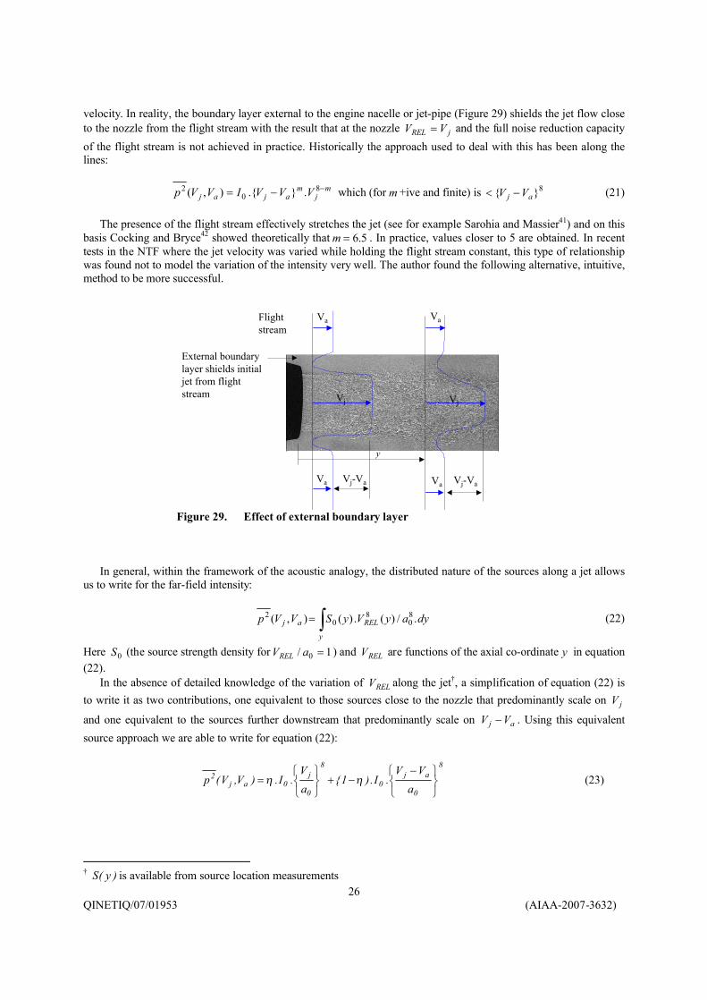
velocity. In reality, the boundary layer external to the engine nacelle or jet-pipe (Figure 29) shields the jet flow close to the nozzle from the flight stream with the result that at the nozzle jREL VV = and the full noise reduction capacity of the flight stream is not achieved in practice. Historically the approach used to deal with this has been along the lines:

mj

majaj VVVIVVp −−= 8

02 .}{.),( which (for m +ive and finite) is 8}{ aj VV −< (21)

The presence of the flight stream effectively stretches the jet (see for example Sarohia and Massier41) and on this basis Cocking and Bryce42 showed theoretically that 5.6=m . In practice, values closer to 5 are obtained. In recent tests in the NTF where the jet velocity was varied while holding the flight stream constant, this type of relationship was found not to model the variation of the intensity very well. The author found the following alternative, intuitive, method to be more successful.

In general, within the framework of the acoustic analogy, the distributed nature of the sources along a jet allows us to write for the far-field intensity:

dyayVySVVp REL

y

aj ./)(.)(),( 80

80

2 ∫= (22)

Here 0S (the source strength density for 1/ 0 =aVREL ) and RELV are functions of the axial co-ordinate y in equation (22).

In the absence of detailed knowledge of the variation of RELV along the jet†, a simplification of equation (22) is to write it as two contributions, one equivalent to those sources close to the nozzle that predominantly scale on jV

and one equivalent to the sources further downstream that predominantly scale on aj VV − . Using this equivalent source approach we are able to write for equation (22):

8

0

aj0

8

0

j0aj

2

aVV

.I.)1{aV

.I.)V,V(p

−

−+

= ηη (23)

† )y(S is available from source location measurements

VjVj

Vj-VaVa Va Vj-Va

External boundarylayer shields initialjet from flightstream

Flightstream

VaVa

y

Figure 29. Effect of external boundary layer

QINETIQ/07/01953 (AIAA-2007-3632)27

Here 0.1≤η and defines the relative contribution of the initial source region effectively shielded by the boundary layer. When η is known, the effect of flight is readily determined in equation (23) from the static intensity 8

0 VR.I . One advantage with this approach is that η provides a direct measure of the extent of the rig’s external boundary layer. In recent tests in the NTF on a newly refurbished (1/10th scale) jet rig20, a comparison of static and flight measurements indicated that 1.0≈η . With the proposed introduction of a boundary layer suction capability, an even lower value for η is anticipated. Because of the stretching effect of the flight stream on the jet flow we might expect η to be a function of aVif the source distribution )( yS is also subject to stretching. However, this is by no means necessarily the case as source location measurements on a subsonic jet, made by the author in the RAE 24ft wind tunnel43, indicated there to be no change in the shape of the source distribution in the presence of the flight stream.

The equivalent source approach described here applies equally to the spectrum of jet noise; allowing us to write for the 1/3rd octave spectral level:

8

0

aj0

8

0

j0aj a

VV.)f(G.)}f(1{

aV

.)f(G.)f()f,V,V(G

−−+

= ηη (24)

- where now, because the high frequency sources of jet mixing noise are relatively close to the nozzle, the quantity η will be some function of frequency. At high frequencies, η may tend to 1 (fully shielded) while at low frequencies it may tend to a small value (towards zero shielding).

B. Effect of Flight on Entropy Noise

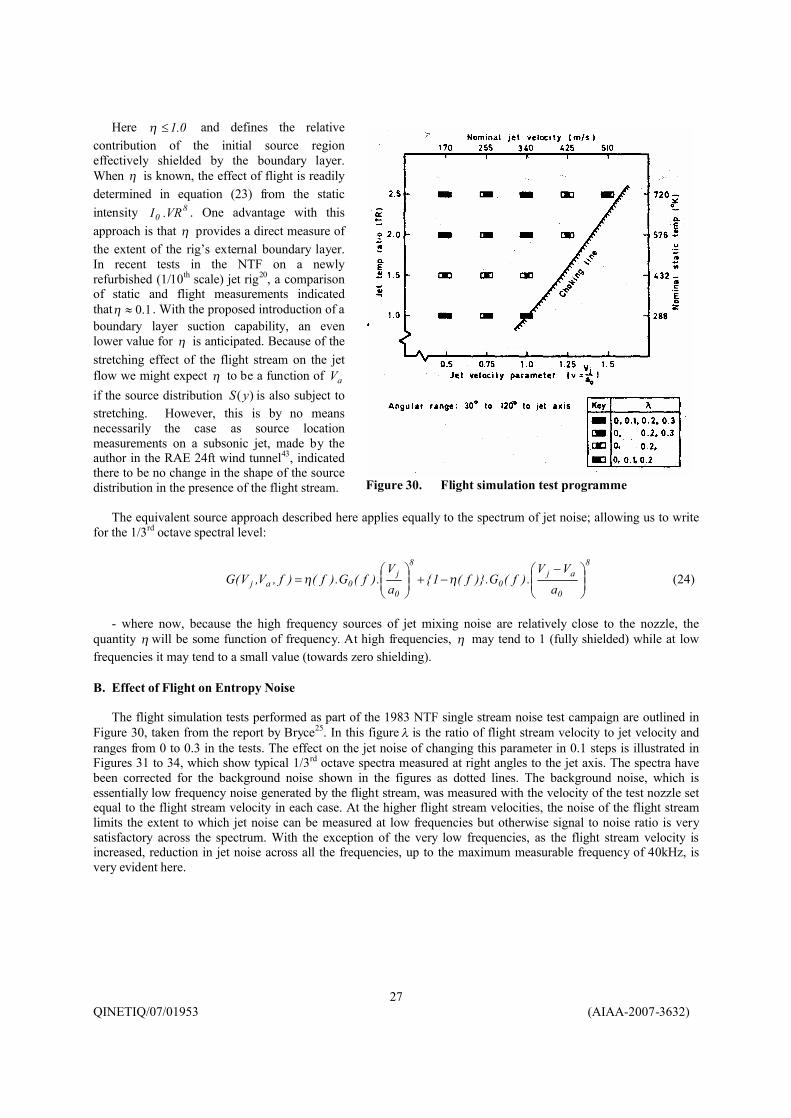
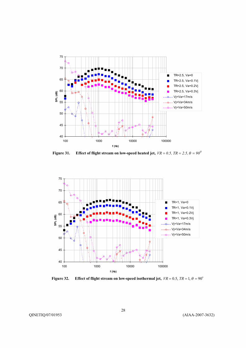
The flight simulation tests performed as part of the 1983 NTF single stream noise test campaign are outlined in Figure 30, taken from the report by Bryce25. In this figure λ is the ratio of flight stream velocity to jet velocity and ranges from 0 to 0.3 in the tests. The effect on the jet noise of changing this parameter in 0.1 steps is illustrated in Figures 31 to 34, which show typical 1/3rd octave spectra measured at right angles to the jet axis. The spectra have been corrected for the background noise shown in the figures as dotted lines. The background noise, which is essentially low frequency noise generated by the flight stream, was measured with the velocity of the test nozzle set equal to the flight stream velocity in each case. At the higher flight stream velocities, the noise of the flight stream limits the extent to which jet noise can be measured at low frequencies but otherwise signal to noise ratio is very satisfactory across the spectrum. With the exception of the very low frequencies, as the flight stream velocity is increased, reduction in jet noise across all the frequencies, up to the maximum measurable frequency of 40kHz, is very evident here.

Figure 30. Flight simulation test programme

QINETIQ/07/01953 (AIAA-2007-3632)28

40

45

50

55

60

65

70

75

100 1000 10000 100000f (Hz)

SPL

(dB

)

TR=2.5, Va=0

TR=2.5, Va=0.1Vj

TR=2.5, Va=0.2Vj

TR=2.5, Va=0.3Vj

Vj=Va=17m/s

Vj=Va=34m/s

Vj=Va=50m/s

Figure 31. Effect of flight stream on low-speed heated jet, 090,5.2TR,5.0VR === θ

40

45

50

55

60

65

70

75

100 1000 10000 100000f (Hz)

SPL

(dB

)

TR=1, Va=0

TR=1, Va=0.1Vj

TR=1, Va=0.2Vj

TR=1, Va=0.3Vj

Vj=Va=17m/s

Vj=Va=34m/s

Vj=Va=50m/s

Figure 32. Effect of flight stream on low-speed isothermal jet, 090,1,5.0 === θTRVR

QINETIQ/07/01953 (AIAA-2007-3632)29

60

65

70

75

80

85

90

95

100 1000 10000 100000

f (Hz)

SPL

(dB

)

TR=2.5, Va=0

TR=2.5, Va=0.1Vj

TR=2.5, Va=0.2Vj

TR=2.5, Va=0.3Vj

Vj=Va=33m/s

Vj=Va=68m/s

Vj=Va=100m/s

Figure 33. Effect of flight stream on high-speed heated jet, 090,5.2,1 === θTRVR

60

65

70

75

80

85

90

95

100 1000 10000 100000f (Hz)

SPL

(dB

)

TR=1, Va=0

TR=1, Va=0.1Vj

TR=1, Va=0.2Vj

TR=1, Va=0.3Vj

Vj=Va=33m/s

Vj=Va=68m/s

Vj=Va=100m/s

Figure 34. Effect of flight stream on high-speed isothermal jet, 090,1,1 === θTRVR

QINETIQ/07/01953 (AIAA-2007-3632)30

50

55

60

65

70

75

0.01 0.1 1 10 100

St=fD/(Uj-Ua)

SPL

(dB

)

TR=2.5, Va=0

TR=2.5, Va=0.1Vj

TR=2.5, Va=0.2Vj

TR=2.5, Va=0.3Vj

TR=2.5, Va=0.1Vj, ETA=0.25

TR=2.5, Va=0.2Vj, ETA=0.22

TR=2.5, Va=0.3Vj, ETA=0.15

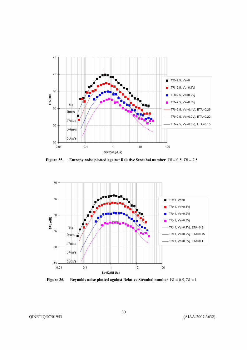
Figure 35. Entropy noise plotted against Relative Strouhal number 5.2,5.0 == TRVR

0m/s

17m/s

34m/s

50m/s

Va

45

50

55

60

65

70

0.01 0.1 1 10 100

St=fD/(Uj-Ua)

SPL

(dB

)

TR=1, Va=0

TR=1, Va=0.1Vj

TR=1, Va=0.2Vj

TR=1, Va=0.3Vj

TR=1, Va=0.1Vj, ETA=0.3

TR=1, Va=0.2Vj, ETA=0.15

TR=1, Va=0.3Vj, ETA=0.1

Figure 36. Reynolds noise plotted against Relative Strouhal number 1,5.0 == TRVR

0m/s

17m/s

34m/s

50m/s

Va

QINETIQ/07/01953 (AIAA-2007-3632)31

50

55

60

65

70

75

0.01 0.1 1 10 100St=fD/Uj

SPL

(dB

)

TR=2.5, Va=0

TR=2.5, Va=0.1Vj

TR=2.5, Va=0.2Vj

TR=2.5, Va=0.3Vj

TR=2.5, Va=0.1Vj, ETA=0.25

TR=2.5, Va=0.2Vj, ETA=0.22

TR=2.5, Va=0.3Vj, ETA=0.15

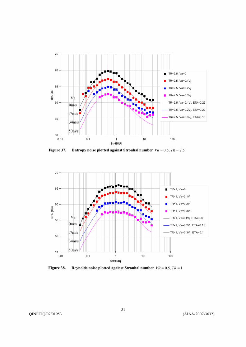
Figure 37. Entropy noise plotted against Strouhal number 5.2,5.0 == TRVR

0m/s

17m/s

34m/s

50m/s

Va

45

50

55

60

65

70

0.01 0.1 1 10 100

St=fD/Uj

SPL

(dB

)

TR=1, Va=0

TR=1, Va=0.1Vj

TR=1, Va=0.2Vj

TR=1, Va=0.3Vj

TR=1, Va=01Vj, ETA=0.3

TR=1, Va=0.2Vj, ETA=0.15

TR=1, Va=0.3Vj, ETA=0.1

Figure 38. Reynolds noise plotted against Strouhal number 1,5.0 == TRVR

0m/s

17m/s

34m/s

50m/s

Va

QINETIQ/07/01953 (AIAA-2007-3632)32

The effect of flight on entropy noise will be explored using the low velocity heated ( 5.2TR,5.0VR == ) data of Figure 31 and for the Reynolds momentum noise, the isothermal data of Figure 32. Figure 31 reveals the peak frequency of this entropy dominant noise to be independent of the flight stream velocity, while that of the momentum noise (Figure 32) appears to reduce with increasing aV (see also Figure 34). The distinct character of the entropy noise spectrum is retained in the presence of the flight stream but reduced in level, as too is that of the flatter Reynolds noise spectrum. It should be pointed out that the reduction in level observed here at right angles to the jet does not occur for rig noise radiated from the nozzle exit (or core noise on an engine). These data are re-plotted against Strouhal number based on RELV in Figures 35 and 36 and against Strouhal number based on jV in Figures 37

and 38. In Figure 35, the momentum spectra appear to all peak at RELV/fD of about 1.3, while in Figure 37, the entropy spectra all peak at jV/fD of 0.5.

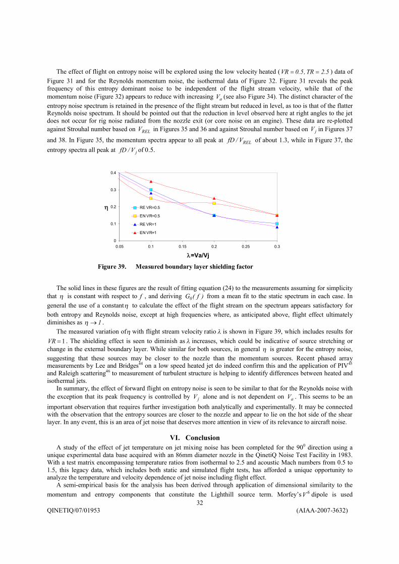
The solid lines in these figures are the result of fitting equation (24) to the measurements assuming for simplicity that η is constant with respect to f , and deriving )f(G0 from a mean fit to the static spectrum in each case. In general the use of a constantη to calculate the effect of the flight stream on the spectrum appears satisfactory for both entropy and Reynolds noise, except at high frequencies where, as anticipated above, flight effect ultimately diminishes as 1→η .

The measured variation ofη with flight stream velocity ratio λ is shown in Figure 39, which includes results for 1=VR . The shielding effect is seen to diminish as λ increases, which could be indicative of source stretching or

change in the external boundary layer. While similar for both sources, in general η is greater for the entropy noise, suggesting that these sources may be closer to the nozzle than the momentum sources. Recent phased array measurements by Lee and Bridges44 on a low speed heated jet do indeed confirm this and the application of PIV45

and Raleigh scattering46 to measurement of turbulent structure is helping to identify differences between heated and isothermal jets.

In summary, the effect of forward flight on entropy noise is seen to be similar to that for the Reynolds noise with the exception that its peak frequency is controlled by jV alone and is not dependent on aV . This seems to be an important observation that requires further investigation both analytically and experimentally. It may be connected with the observation that the entropy sources are closer to the nozzle and appear to lie on the hot side of the shear layer. In any event, this is an area of jet noise that deserves more attention in view of its relevance to aircraft noise.

VI. ConclusionA study of the effect of jet temperature on jet mixing noise has been completed for the 900 direction using a

unique experimental data base acquired with an 86mm diameter nozzle in the QinetiQ Noise Test Facility in 1983. With a test matrix encompassing temperature ratios from isothermal to 2.5 and acoustic Mach numbers from 0.5 to 1.5, this legacy data, which includes both static and simulated flight tests, has afforded a unique opportunity to analyze the temperature and velocity dependence of jet noise including flight effect.

A semi-empirical basis for the analysis has been derived through application of dimensional similarity to the momentum and entropy components that constitute the Lighthill source term. Morfey’s 6V dipole is used

0

0.1

0.2

0.3

0.4

0.05 0.1 0.15 0.2 0.25 0.3

λ=Va/Vj

η RE VR=0.5

EN VR=0.5

RE VR=1

EN VR=1

Figure 39. Measured boundary layer shielding factor

QINETIQ/07/01953 (AIAA-2007-3632)33

successfully for the entropy noise, with strength proportional to the entropy difference across the shear layer. Using this approach, the spectra measured at constant velocity for different temperatures have been successfully analyzed, separating the momentum and entropy contributions, which are assumed to be uncorrelated in this study. Because the density in a heated jet varies across the shear layer, an iterative process has been adopted to determine the appropriate source density, which is found to vary from the geometric mean density at low velocities, to the core density at high velocities, indicating the dominant source region to be on the hot side of the shear layer.

The extracted entropy spectra scale on six powers of jet velocity and peak at a Strouhal number of 0.5 while the momentum spectra scale on eight powers and peak at a Strouhal number of 1.3. Using the master spectra so obtained for the two components in the dimensional model, good agreement with the spectral measurements has been demonstrated across the temperature and velocity range of the tests. The increase in mixing noise at low velocities with heating is well replicated and likewise the reduction at high velocities. In addition, the model provides a clear explanation for the observed variation of the OASPL with temperature and velocity. A surprising result is the extent to which entropy noise remains a significant component as jet velocity increases. At the highest velocity and temperature in the tests )5.2TR,5.1VR( == entropy is found to increase the overall noise by 2dB relative to the momentum contribution while halving the peak frequency in the process. Thus it is not sufficient to derive a noise spectrum for a heated high-speed jet from an isothermal or unheated spectrum alone (of the same velocity), adjusted in level for density.

In the presence of a flight steam, entropy noise is shown to reduce in level in much the same way as the momentum noise but without change in its characteristic frequency, which is a significant observation. A new semi-empirical method for the modelling of flight effect, that introduces directly boundary layer shielding, indicates that the entropy noise sources may be closer to the nozzle than the momentum sources.

Within the framework of the Lighthill acoustic analogy, this study has confirmed the existence of an entropy type noise source in heated jets that is separate from the momentum noise and apparently uncorrelated with it. The evidence indicates that the presence of entropy noise is not a quirk of low Reynolds number. However, further research, both experimental and theoretical, is needed if we are to properly understand the turbulent generation mechanism behind this important component of jet noise.

AcknowledgementsThe author wishes to thank Richard Pinker of QinetiQ for assistance with information on the NTF tests and Paul

Strange of Rolls-Royce for useful discussions during the course of this work.

References1Lassiter L.W. and Hubbard H.H., “Experimental Studies of Noise from Subsonic Jets in Still Air,” NACA TN-2757, August.

1952.2Rollin V.G., “Effect of Jet Temperature on Jet Noise Generation”, NACA TN-4217 March 1958. 3Fitzpatrick H.M. and Lee R., “Measurements of Noise Radiated by Subsonic Air Jets,” Navy Department Report 835,

November 1952.4Westley R. and Lilley G.M., “Investigation of the Noise Field from a Small Jet and Methods for its Reduction”, Cranfield

Report No. 53, January 1952.5Smith M.J.T., “Aircraft Noise”, Cambridge Aerospace Series, ISBN 0-521-33186-2, 1989.6Lighthill M.J., “On Sound Generated Aerodynamically”, Parts I. and II, Proceedings of the Royal Society of London 1952

and 1954.7Lighthill M.J., “The Bakerian Lecture 1961, Sound Generated Aerodynamically”, Royal Aircraft Establishment, Tech.

Memo No DIR. 8, November 1961.8Lighthill M.J., “Jet Noise”, AGARD Rep 448, 1963.9Lilley G.M. Westley R. and Young A.D., “Noise Suppressing Nozzles for Aircraft Jet Propulsion Engines”, Patent

Specification 766,986, January 1957.10Banerian G., “Status Review of Jet Noise”, AIAA 77-1262, 4th AIAA Aeroacoustics Conference, 3-5 October 1977,

Atlanta, Georgia.11Bodony D.J. and Lele S.K., “Jet Noise Prediction of Cold and Hot Subsonic Jets Using Large-eddy Simulation”, AIAA-

2004-3022, 10th AIAA/CEAS Aeroacoustics Conference, 10-12 May 2004, Manchester, UK.12Lew P., Blaisdell G.A. and Lyrintzis A.S., “Recent Progress of Hot Jet Aeroacoustics Using 3-D Large-Eddy Simulation”,

AIAA-2005-3084, 11th AIAA/CEAS Aeroacoustics Conference, 23-25 May 2005, Monterey, California.13Tristanto I.H., Page G.J, and McGuirk J.J., “Large Eddy Simulation of Hot Coaxial Jets”, AIAA-2006-2497, 12th

AIAA/CEAS Aeroacoustics Conference, 8-10th May 2006, Cambridge, Massachusetts.14Moore P. and Boersma B.J., “Investigation of the noise from cold and heated subsonic jets”, AIAA 2006-2500, 12th

AIAA/CEAS Aeroacoustics Conference, 8-10th May 2006, Cambridge, Massachusetts.15Khavaran A, and Kenzakowski D.C., “Progress Toward Improving Jet Noise Predictions in Hot Jets”, AIAA-2007-12, 45th

AIAA Aerospace Sciences Meeting and Exhibit, 8-11 January 2007, Reno, Nevada.

QINETIQ/07/01953 (AIAA-2007-3632)34

16Lew P-T., Blaisdell A. and Lyrintzis A.S., “Investigation of Noise Sources in Turbulent Hot Jets using Large Eddy Simulation Data”, AIAA-2007-16, 45th AIAA Aerospace Sciences Meeting and Exhibit, 8-11 January 2007, Reno, Nevada.

17Cai X., Ladeinde F. and Alabi K., “Towards Predicting Supersonic, Hot Jet Noise”, AIAA-2007-826, 45th AIAA Aerospace Sciences Meeting and Exhibit, 8-11 January 2007, Reno, Nevada.

18Ahuja KK, ‘Designing clean jet-noise facilities and making accurate jet-noise measurements’, Aeroacoustics, vol. 2 number 3 & 4, pages 371-412, 2003

19Vishwanathan K, “Jet aeroacoustic testing: issues and implications’, AIAA Journal vol. 41 No. 9, September 2003.20Pinker RA, “The Enhancement of the QinetiQ Noise Test Facility for Larger Scale Exhaust Systems”, AIAA-2004-3019,

May 2004, Manchester, UK21Bridges J. and Brown C.A., “Validation of the Small Hot Jet Acoustic Rig for Aeroacoustic Research”, AIAA 2005-2846,

11th AIAA/CEAS Aeroacoustics Conference, 23-25 May 2005, Monterey, California.22Harper-Bourne M., “Jet Noise Measurements”, Experimental Aeroacoustics, Lecture Series 2007-01, von Karman Institute

for Fluid Mechanics, November 2006, Brussels.23Tanner H.K., “An Experimental Study of Jet Noise I: Turbulent Mixing Noise”, Journal of Sound and Vibration, 50, No. 3,

405-428, 1977.24Cocking B J, “The Effect of Temperature on Subsonic Jet Noise”, National Gas Turbine Establishment, NGTE Rep. R. 331,

May 197425Vishwanathan K, “Aeroacoustics of hot jets”, JFM (2004), vol. 516, pp. 39-8226Bryce W.D., “The Prediction of Static-to-Flight Changes in Jet Noise”, AIAA 84-2358, 9th AIAA/NASA Aeroacoustics

Conference, 15-17 October 1984, Williamsburg, Virginia.27Pinker R.A., “Results from an experimental programme on static single-stream jet noise”, QinetiQ/FST/TN026455, 2003.28Morfey C.L., “Amplification of aerodynamic noise by convected flow inhomogeneities”, Journal of Sound and Vibration,

(1973) 31(4), 391-397.29Poudman I., “The Generation of Noise by Isotropic Turbulence”, Proc. Roy. Soc. A.214, 119-132, 195230Tam C.K.W., Viswanathan K., Ahuja K.K. and Panda J., “The Sources of Jet Noise: Experimental Evidence”, AIAA 2007-

3641, 13th AIAA/CEAS Aeroacoustics Conference, May 2007, Rome.31Harper-Bourne M., “Jet Noise Turbulence Measurements”, AIAA-2003-3214, 9th AIAA/CEAS Aeroacoustics Conference,

May 2003, South Carolina.32Ribner H.S., “The generation of sound by turbulent jets”, Advances in Applied Mechanics, Vol. 8 (1964).33Bushell, K.W., “A Survey of Low Velocity and Coaxial Jet Noise with Application to Jet Prediction”, Symposium on

Aerodynamic Noise, 14-17 September 1970, Loughborough University of Technology, England. 34Lush P.A. and Fisher M.J., ‘Noise from hot jets’, Proceedings of the AGARD conference on noise mechanisms, Brussels

September 1973.35Fisher M.J., Lush P.A. and Harper-Bourne M., ‘Jet Noise’, Journal of Sound and Vibration, (1973) 28(3), 563-585.36Boersma B. J., “Large Eddy Simulation of the sound field of a round turbulent jet,” Theor. Comp. Fluid. Dyn., Vol. 19,

2005, pp. 161–170.37Ribner HS, ‘Basic aerodynamic noise research’, NASA SP-207, July 196938Tanna H.K., Fisher M.J. and Dean P.D., “The influence of temperature on shock-free supersonic jet noise”, Journal of

Sound and Vibration (1975) 39(4), 429-460.39Bazley E N, “Sound absorption in air at frequencies up to 100kHz”, NPL Acoustics Report AC74, February 1976.40Bhat T.R.S., “Reynolds Number and Temperature Effects on Jet Noise”, AIAA-2007-3630, 13th AIAA/CEAS

Aeroacoustics Conference, 21-23 May 2007, Rome, Italy41Sarohia V. and Massier P.F., “Effects of external boundary layer flow on jet noise in flight”, AIAA 76-558, AIAA Aero-

Acoustics Conference, 20-23 July 1976, Palo Alto, California.42Cocking B.J. and Bryce W.D., “Subsonic jet noise in flight based on some recent wind-tunnel results”, AIAA 75-462, 2nd

AIAA Aeroacoustics Conference, 24-26 March 1975, Hampton Virginia.43Harper-Bourne M., “The Distribution of Jet Noise Sources Using Far-Field Microphones”, AIAA-98-2357, 4th

AIAA/CEAS Aeroacoustics Conference, 2-4 June 1998, Toulouse.44Lee S.S. and Bridges J., “Phased-array Measurements of Single Flow Hot Jets”, AIAA 2005-2842, 11th AIAA/CEAS

Aeroacoustics Conference, 23-25 May 2005, Monterey, California.45Bridges J., “Effect of Heat on Space-Time Correlations in Jets”, NASA/TM-2006-214381, September 2006, AIAA-2006-

2534, 12th AIAA/CEAS Aeroacoustics Conference, 8-10th May 2006, Cambridge, Massachusetts.46Panda J., Seasholtz R.G., Elam K.A., Mielke A.F. and Eck D.G., “Effect of Heating on Turbulent Density Fluctuations and

the Noise Generation From High Speed Jets”, NASA/TM-2004-213126, AIAA-2004-3015, 10th AIAA/CEAS Aeroacoustics Conference, 10-12 May 2004, Manchester, UK.