Buoyancy-driven asymmetric water boundary layer along a heated cylinder

J . Fluid Mech. (1980), vot. 98, part 2, p p . 417-434

Pkmted in &eat Britain 417

Bouyancy-driven asymmetric water boundary layer along a heated cylinder

By LUN-SHIN YAO Department of Mechanical and Industrial Engineering,

University of Illinois at Urbana-Champaign, Urbana, IL 61801

IVAN CATTON AND J. M. McDONOUGH University of California, Los Angeles, CA 90052

(Received 9 August 1978 and 9 October 1979)

The development of a three-dimensional water boundary layer along a heated longitudinal horizontal cylinder is studied by a finite-difference method. The secondary flow is induced in an otherwise axially symmetric laminar boundary layer by the buoyancy force. The development of the boundary layer is studied under two heating conditions: constant wall heat flux and constant wall temperature. In general, close to the leading edge, the magnitude of the secondary flow is small and the boundary-layer flow is forced-convection dominant. The secondary flow grows downstream, and the interaction of the free and forced convection becomes important. The flow becomes free-convection dominant further downstream. The temperature-dependent viscosity of water has the effect of thinning the heated boundary layer. The buoyancy effect and the variable viscosity effect enhance each other over the lower part of the cylinder and compete with each other over the upper part of the cylinder. The numerical results compare with the forced convection dominant asymptotic solution and indicate that the asymptotic solution is only valid when x < O.la/d. Since the boundary layer is thin compared with the radius of the cylinder, the transverse curvature effect is small and can be neglected. Therefore, the solution can be applied to the entrance region of heated straight pipes as the zeroth-order boundary-layer flbw.

1. Introduction Axisymmetric forced-convection laminar boundary layers exist on various engi-

neering apparatus and have been extensively studied for the past half century. The effects of buoyancy-induced secondary flow, which may destroy the axisymmetry of the laminar boundary layer over an axisymmetric body, has received little attention. Recently, some perturbation solutions have been obtained for both external flow (longitudinal cylinders or cones) by Yao & Catton (1977, 1978) and internal flow (pipe flow) by Yao (1978a, b ) . Although the perturbation solutions are only valid in a narrow region close to the leading edge of an axisymmetric body (or the entry region of a pipe), the results indicate that the classical Nusselt-number correlations, which do not con- sider the asymmetric secondary-flow effect, can be in large error. However, the size of upstream region where the perturbation solution can be applied is unknown. The downstream solution, where the secondary flow cannot be treated as a perturbed

0022-1 120/80/4453-1110 $02.00 @ 1980 Cambridge University Press

14 T L M 98

418 L.4 . Yao, I . Catton and J . M . McDonough

quantity, is needed for many practical applications. This paper gives the downstream numerical solution.

The temperature-dependent viscosity of water provides a mechanism by which laminar flow can be maintained by wall heating. The stabilization results because the velocity profiles under the surface heating inhibit the amplification of Tollmien- Schlichting instability waves and thus retard boundary-layer transition. This has been verified by the experiments of laminar pipe flow (Barker & Jennings, 1977). Currently, very little three-dimensional stability theory is available. Before any such theory can be developed, accurate three-dimensional velocity profiles are required. In this paper a finite-difference method is used to solve the three-dimensional boundary-layer equations. The results will provide three-dimensional velocity to flow stability analyses as well as heat transfer correlations.

The physical model considered is a semi-infinite cylinder of radius a, which is aligned with its axis parallel to a uniform free stream and normal to the direction of gravity. The free stream is assumed to have a velocity u, and temperature T,. Two surface heating conditions are studied. One is the constant surface temperature Tw(Tw > T,). The other is constant surface heat flux, qw. For water flow in the range of 4.4 and 45 "C, the principal departure from constant property flow is due to viscosity variation. The empirical correlation of water viscosity used in this study will be described in the text. Further, within this temperature range, the density variation is small and the Bous- sinesq approximation for the buoyancy force is used.

The boundary-layer thickness is shown to be proportional to a Gr-4 (constant wall temperature) or a Qr-4 (constant wall heat flux), where Gr and Br are Grashof numbers and are defined in equations (2) and (8), respectively. Since the boundary layer is thin for a large Grashof number, the transverse curvature effect is higher order. Therefore, the lowest-order boundary-layer solutions are identical for ext(erna1 and internal flows; the solution presented in the paper can then be taken as the zeroth-order boundary-layer flow in the entrance region of heated straight pipes. It has been recognized (see Yao 1978) that there are similarities between the flows in a heated straight pipe and in a curved pipe. In the test, we shall point out the similarities.

A careful comparison of the numerical results with the perturbation solution shows they are identical for E 6 0. l a / d ( B is defined in equation (2)). Two solutions, however, start to deviate at 5 = O.la/d. This indicates that the perturbation solution is only valid within a small distance from the leading edge. The downstream solution is uniformly valid from the leading edge; therefore, the composite expansion is not necessary for this problem. Similarly, the asymptotic solution of the flow in the entry region of a curved pipe (Singh 1974) is valid whenZ(cd/a) is small, where a is the curvature ratio of curved pipes.

For x > 1-6a/d, the fluid is sucked into the boundary layer along the bottom of the cylinder; the boundary layer grows drastically along the top of the cylinder. Even- tually, the free convection becomes a dominant mode. The buoyancy effect for the constant surface heat flux condition is smaller than that for the constant surface temperature condition when x is small. Further downstream, the buoyancy effect becomes stronger for the constant surface heat flux case. The temperature-dependent water viscosity thins the boundary when it is heated. This increases the heat transfer rate but decreases the buoyancy effect.

A water boundary layer along a heated cylinder

x = ?&/a, r = (? -a ) G d / a the co-ordinates;

0 = T-T,/AT, AT = T,-T, the temperature;

Re = u,a/v,

Gr = pga3(T, - T,)/v2

the Reynolds number;

the Grashof number;

419

)

2. Analysis The governing equations for longitudinal flow with variable viscosity on a heated,

horizontal cylinder are the Boussinesq boundary-layer equations. I n cylindrical co-ordinates, as shown in figure 1, they are

au 1 a(?;@ 1 av -+I- +=- = 0, ax r a?; r a$

-8T EaT -aT a2T u-+= -+w- = a-. az r a$ a?; a r 2

The variables are defined in equations (2) and (8).

420 L.-8. Yao, I . Catton and J . M . McDonough

Here $ is the thermal expansion coefficient and v is the kinematic viscosity. The subscript m denotes the quantity associated with the free stream. The longitudinal length scale was chosen as ale4 which is derived from the upstream asymptotic solution. The asymptotic solution is valid over a distance O(a) from the leading edge where the magnitude ofthe secondary boundary layer, O(e) , is very small and can be treated as a perturbed quantity. However, the asymptotic sylution indicates that the order of the secondary boundary layer increases to O(e3) at adistance of O(ale4) from the leading edge. Even though the magnitude of the secondary boundary layer is still much smaller than that of the longitudinal flow, the interaction between them cannot be ignored. This is the reason why the asymptotic solution in the region, X - O(a), breaks down. The co-ordinate normal to the wall has been stretched t o reflect the fact that the thickness of the boundary layer in the region X - O(a/eJ) is proportional to aGr-). This thickness of the boundary layer in this region is much larger than the boundary-layer thickness, O(Re-)), in the region X - O(a) when e is small. However, it is still very thin compared with the radius, a, of the cylinder. Hence, the transverse curvature effect can still be neglected. In fact the transverse curvature effect can be demonstrated to be the order of Gr-t; but it may become important as the boundary layer grows thick further downstream. The axial length scale of the further downstream region may be a Re where the thickness of the boundary layer is the same order as the radius of the cylinder. The scaling law is somewhat similar to the entry flow in a pipe whose wall temperature is held constant (see Yao, 1978b). However, the exact location that the transverse curvature effect cannot be ignored can only be found by comparing the numerical solution with the further downstream solution which is, unfortunately, not available a t present.

In terms of the dimensionless variables in equation (2), equation (1) become

au av aw -+-+- = 0) ax a$ ar

au au au

av av av ax a# ar

u-+v-+w- =

2 = O(s) , ar

( 3 4

( 3 4

N represents the temperature-dependent viscosity of water and is defined the same as by Yao & Catton (1978)) and will be briefly summarized later.

Notice that equation ( 3 4 implies that the pressure gradient normal to the wall is negligible. It also is worthy to point out that equations (3) are very similar to the boundary-layer equations of an entry flow in curved pipes with the limit that the curvature ratio of curved pipes approaches zero (see Yao & Berger 1975). The only difference between equations (3) and those for curved pipes is that the body force for

A water boundary layer along a heated cylinder 42 1

heated-pipe flows is the buoyancy force, and that for curved-pipe flows is the centri- fugal force.

For the numerical computation of the boundary layer, it is convenient to use parabolic co-ordinates (see Smith & Clutter 1963; Dwyer 1963). Equations ( 3 ) in (x, q = r/(2x)t,+) can be expressed

The matching conditions between the solutions of the region O(a/s*) and the region O(a) can be easily derived by applying asymptotic matching principles (see Van Dyke, 1964) to the asymptotic solution in the region of O(a) .

For the case of constant wall temperature, they are

where q = r/(2x)3 is the Blasius variable, and the stream function fo, PI, F2 and temperature functions 8,, and G, are defined by Yao & Catton (1977, 1978). It is interesting to note that the growth of the boundary-layer thickness along the longitudinal direction is proportional to Re-3 in both regions of O ( a ) and O ( a / s t ) .

The boundary conditions resulting from merging the boundary layer with the free stream are

u + l , v and B+O as 7 3 ~ 0 . ( 6 a )

A t the wall, the velocity meets the no-slip condition, and the temperature is constant. The resulting boundary conditions are

u = v = w = 0 and 8 = 1 (constant temperature), at q = 0. ( 6 b )

Along the symmetry line, the conditions are

= 0, at 4 = 0. au aw a6

v = o , - - a # - @ = @

422 L.-S. Yao, I . Catton and J . M . McDonough

Values of the dependent variables are required along q5 = 0 to start the numerical computation at each x station. The equations that govern the flow along q5 = 0 can be obtained by taking the limit of equations (4) according to equation (6c). This gives

where (7c) is obtained from (4c) by differentiation with respect to $ before taking the limit q5 + 0.

2.2. Constant wall heatJlux

Dimensionless variables for a constant wall heat flux flow are slightly different from those for a constant wall temperature. They were suggested by the upstream asymptotic solution (see Yao 1978a, b ) and are

u = Flu,, v = %/urn&, w = i$%t/u,.E* the velocities;

x = ZEf/a, r = F - a&%*/a the co-ordinates;

8 = q,,, = T - T,/AF, AT = ka&/aq, the temperature;

Re = u,a/v the Reynolds number;

= pga4qw/kv2 the Grashof number;

Pr = v,/a the Prandtl number;

N = v/va the viscosity ratio;

E = &/Re#.

Use of the dimensionless parameters given by equations ( 8 ) in equations (1) results in equations (3). In other words, the dimensionless equations of motion and energy are the same for both constant wall temperature and constant wall heat flux flows. How- ever, the physical meanings are not identical.

The boundary conditions for constant wall heat flux are essentially equations (6a), (6 b) and (6 c ) with

( 6 4 ae - = - ( 2 ~ ) ) at 7 = 0 a7

replacing 8 = 1 in equation ( 6 b ) . The matching conditions between the solutions of the upstream region O(a) and the

downstream region O(a/s%) can be derived from the upstream asymptotic solution. They are

u1 = fk(7) + (2x)W;(7) cos $ + . . . , 2rl = ( ~ x ) t ~ L ( q ) sin 4 + . . . ,

e = (244 . [eo(7) + ( 2 4 t ~ , ( ? j ) cos q5 + ...I.

( 9 4

(9b)

(94

( 9 4

( ~ Z ) * W , = (dk(7) - f o ( ~ ) ) + ( 2 x ) % ( ~ % ( q ) - 6 F l ( ~ ) -p2(7)) COS+ +

A water boundary layer along a heated cylinder 423

The stream functions,f,, Fl and F2 and the temperature functions 8, and G, are defined in Yao (1978) . The upstream solutions ( 9 ) are for constant property fluid only. A method to extend the solutions to variable property flow will be described below.

On examining the upstream conditions (5) and ( 9 ) , one finds that the upstream conditions a t x = 0 are simply Blasius velocity profiles with energy transfer. D y e r (1968) showed that the upstream conditions can also be obtained by solving the limiting equations ( 3 ) as x + 0 . They are

au a a7 a7

? ) - - - - [ (22 ) iw] = 0,

aU ;(ivg) + [ q u - ( z X ) + w ] - = 0,

; (iv$) + [qu - (2X)+W] - = 0,

87

av a7

a2e ae 87

- + Pr[Tu - (Zx)+w] - = 0.

It is obvious that the solution of equations (10) is the Blasius solution with heat transfer which is corresponding to (5) for constant wall temperature and ( 9 ) for constant wall heat flux a t x = 0. This indicates that the upstream asymptotic solution is included in the downstream solution presented in this paper. Numerical computation is started by solving (10) at 2 = 0. The details are described in the following section. Similar interpretation is true for the entry flow in curved pipes, i.e. the upstream asymptotic solution (Singh 1974) is included in the downstream solution (Yao & Berger 1975). However, the solution given by Yao & Berger is an approximate integral solution. No direct comparison between the two solutions is possible.

3. Numerical method We begin discussion of the numerical treatment of the problem by observing that

all of equations (4) are of the same form except for the continuity equation ( 4 a ) . Equations ( 4 b , c, d ) are nonlinear parabolic equations which, although corresponding to steady state, may be,viewed as evolution equations in the streamwise direction (and, in fact, also azimuthally). Thus, it can be expected that some care must be exercised in choosing, a difference approximation in order to avoid numerical instabilities. The difference scheme employed for equations ( 4 b , c , d ) is fully implicit, and although unconditional stability has not been proved, results of rather extensive numerical experiments indicate stability over the entire range of practical (in terms of storage and computation time) meshes.

Equation ( 1 1 ) is the form of the difference approximation for equations ( 4 b , c , d ) with equations ( 1 2 ) and (13 ) providing the explicit information needed to construct the coefficients A(i , m), i = 1 , 2 , 3 , and B(m);

424

where

and

L.-S. Yao, I . Catton and J . M . McDonough

,&%l+l v p l

A(2, m) = - (b, + bm+l)npz+l - ( 2 x ) . ( A [ T ) ~ (x + T) ,

0,

- (2x) 6 sin q5, for equations ( 4 b ) and ( 4 d ) ,

H = { for equation ( 4 c ) ,

for equations ( 4 b ) and ( 4 c )

for equation ( 4 d ) .

N ( 6 ) ,

In equation ( 1 l) , the grid function ($23 corresponds to any of u, v, or 6, according to the step of the computational algorithm (see below) being calculated. The m subscripts label the 7 direction of the mesh while the n superscripts correspond to the x direction; and the 1 superscripts denote the q5 direction. The differencing is first-order in the x direction and second order in the 7 and 4 directions. We note that the mesh star for the discretization used here is very similar to that given by Keller (1975). However, we retain the second-order form of the original differential equations ( 4 ) rather than replace them by an equivalent first-order system. As a consequence, our second-order centred differences lead to skipping over mesh points in first derivative approximations as is typical for centred difference approximations. But this is generally of con- cern only in regions of recirculting flow. The continuity equation ( 4 a ) can be rewritten as

where i.5 = (2x ) )w . The right-hand side of equation (14 ) is independent of W except implicitly through coupling with u and v. Thus, if a t any grid point ( x , #), u and v have already been determined for all [T, we have

di5 - = 9(7), W ( 0 ) = 0 d7

which is just an ordinary differential equation initial value problem. Because the equations for u, v, and 6 have been approximated with second-order differencing in 7, we use the trapezoidal rule to integrate ( 1 4 ) . Hence, the difference equation is

(15) - Wm+1 = w, + (W7) [F(Trn) + 9(7?%+1)1-

The derivatives appearing in .F are approximated consistently with the differencing used in the respective directions in the difference equations (1 1).

As noted above, the numerical scheme has undergone thorough testing to verify stability and convergence rates (of the grid functions) and to determine grid spacing requirements for a prescribed level of accuracy. Stability and theoretical convergence rates have been completely confirmed.


for the results reported in the next section. This leads to roughly two decimal place accuracy (the actual accuracy is somewhat better due to the form of the convergence criterion). The error is bounded by 2 per cent, except along the top of the cylinder where the error is slightly larger and can be as much as 5 % due to the ever-increasing magnitude of normal velocity. The numerical experiments indicate that the following uniform mesh leads to truncation errors which are smaller than Ax = 0.05, A7 = 0.1, and A$ = in. The mesh used to obtain the results reported in the next section was somewhat finer than that needed to produce the desired accuracy: A7 = 0.04, A# = An, and variable Ax, gradually varying from 0.005 near the leading edge (until x = 0.2) to 0.05 from x = 0.6 to x = 2.0.

Equations (4b,c ,d) are nonlinear but as often seems to be the case for boundary layer equations (at least those expressed in similarity variable form), even the simplest form of linearization proved quite adequate for their solution. In particular, the coefficients of equation (1 1) are evaluated at the previous iteration, or at the previous x step for the first iteration of a new step in the x direction. For the level of accuracy to which computations were carried, between two and ten iterations were required; however, this did not increase significantly even for error tolerances of E = Con- vergence appears to be approximately linear with one decimal place of accuracy being gained with each iteration beyond a certain point in the iterative sequence. An excep- t,ion to this occurs in the region where the vertical velocity begins to increase rapidly in the downstream direction (see figure 8). Beginning a t approximately x = 0.85 at least ten iterations were required a t $ = 180" for B = 10-2.

Calculations are started a t x = 0 where the flow is axisymmetric. The corresponding initial conditions are obtained by solving the difference analogues of equations (10). To advance to the next downstream x location, first the symmetry line equations (7) are solved a t the new x location. It is important to observe that these equations depend only on x and 7, provided we differentiate the #-momentum equation with respect to q5, and solve for av/a#, rather than for v. (Since v = 0 a t # = 0, it is only that is of interest anyway.) After the symmetry line conditions have been found, calculations proceed in the azimuthal direction using the difference equation (11) . At each (x, 9) mesh point, a two-point boundary value problem is solved in the 7 direction. This continues around the cylinder up to, and including Q, = 180". Numerical results show that the symmetry condition along $ = 180" is satisfied automatically due to the symmetric form of the buoyancy force which is proportional to sin #; see equation (4c).

Finally, we point out that the system of difference equations (1 1) corresponding to u, v and 8 is decomposed and solved blockwise. This reduces the storage requirement for the matrix of coefficients for the difference equations and in addition, the complexity of the solution algorithm is decreased. In particular, each separate block (associated with one of u, v , or 0) results in a tridiagonal system which can be stored in less than 4M storage locations where M is the number of 7-grid points. Moreover, each such system can be solved in O ( M ) arithmetic operations using, for example, tridiagonal Gaussian elimination.

Algorithm: Assumej- 1 iterations have been completed. Then for the j th iteration,

evaluate A(i , m) and B(m).

It was decided to employ an iteration convergence tolerance, B =

The computational algorithm at each (x - 6) location is the following.

(1) Solve equation (1 1) with {@zz) = {uzz) v, w , and 8 from the previous iteration to

426 L.-S. Yao, I . Catton and J . M . McDonough

(2) Solve equation (1 1) with {$zz} = {v$} using w, 8 from the previous iteration and

(3) Solve equation (16) for (wzz} using u,v from steps 1 and 2, respectively. (4) Solve equation (1 1) with ($2;") = {8$} using u, v, and w from the preceding three

u from step 1.

steps. ( 5 ) Test convergence using {max Jug) - u%-l)I + max - v2-l) I

rlm rlm

+ max I wz) - wg-l) I + max I eg) - Og-1) I} < E, rlm

where ?ln,e[O, 7max], and for results presented below, vmax = 10. (6) If convergence is achieved, proceed to next q5 location; if not, incrementj and

go to step 1.

4. ResuIt and discussion Two surface heating conditions are computed : the constant surface temperature

and the constant surface heat flux. The model of the water viscosity ratio is specified, before the solutions are presented. It can be shown that the viscosity of water (see Yao & Catton 1978) in the range of temperature 4.4 "C and 45 "C can be approximated bY

' l + a A T 8 , (16) r -7 - where a = 0.0272.

mated by The Prandtl number of water in the same range of temperature can be approxi-

Pr = 455/(32 + 1.8 T!), (17)

where T, is in "C. The illustrative calculations described below are performed using a value of Pr = 8. This value is large enough to ensure that a small increase of Pr does not cause much change of the numerical results. The conditions of overheating are selected for a A T = 0.5 and 1.0 which correspond to A T = 18.38 "C and 36.76 "C.

4.1. Velocity distribution The axial velocity profile at x = 0 is plotted in figure 2. The diminution of water viscosity by heating makes the velocity profile fuller a t a higher heating level. For the condition of constant surface heat flux, the fluid temperature at x = 0, equals the free-stream temperature, i.e. 8 = 0. Therefore, the velocity profile is simply a Blasius profile which coincides with that of a = 0 (constant water viscosity).

Downstream from the leading edge, say x = 1, the axial velocity profile developes to accomodate the secondary flow effect in order to satisfy the mass conservation. The velocity profile becomes fuller, figure 3, and the boundary layer is thinned, figure 4, by the secondary flow along the lower surface of the cylinder. The fluid, which is carried along the cylinder by the buoyancy force, accumulates in the neighbourhood of the top of the cylinder. This thickens the boundary layer and decreases the curvature of the velocity profile. The buoyancy force seems proportional to the total heat input. For the case of constant wall heat flux, the effect of buoyancy is smaller than that of the constant wall temperature when xis small. Also, as shown in figures 3 and 4, the boundary

5 -

4 -

427

layer is thinned owing to the decrease of the water viscosity; and the axial velocity profile becomes fuller when the cylinder is heated. The variable viscosity effect can be demonstrated clearly by the fact that the displacement thickness of the boundary layer has a sharp drop between x = 0 and x = 0.1 for qw = constant; see figure 4. When aAT = 0.5, the buoyancy force starts to increase the displacement thickness at x = 0.4. When aAT = 1-0, this occurs at x = 0.6. In general, over the lower part of the cylinder, the secondary flow and the variable viscosity enhance each other; over the upper part of the cylinder, they compete with each other. The boundary of the enhancing region and the competing region starts at q5 = 90" when x = 0 and increases to larger q5 downstream.

It can be shown that the axial shear stress, 7zr can be expressed as

for both Tw = constant and qw = constant. The normal gradient of the axial velocity on the wall, au(O)/aq, is given in figure 5.

Figure 5 shows that the thinning of the boundary-layer thickness owing to the variable viscosity and the secondary-flow effects increases the axial velocity gradient normal to the wall. In the neighbourhood of q5 = 180°, this gradient drops fast owing to the thickening of the boundary layer. For x < 1.5, the effect of the buoyancy force for qw = constant is smaller than that of Tw = constant. However, the buoyancy effect of qw = constant increases faster downstream than that of T, = constant. This implies


-u (qw = constant)

1 , .o 0;8 0;6 0;4 0;’

4 k

0 0.2 0.4 0.6 0.8 1 .o u (T, = constant)

FIQURE 3. Axial velocity at x = 1. See figure 2 for the symbols.

FIQURE 4. Displacement thickness. See figure 2 for the symbols.


x (4, = constant) 1 .s 1 .o 0.5 0

1.0'

0.5

0.1 0 0.5 1 .o 1.5

FIGURE 5. Axial velocity gradient along the surface (the lines with dots are for T, = constant).

that the buoyancy effect for qw = constant can grow larger further downstream than that of T, = constant.

Equations (5a) and (9a ) indicate that the axial velocity profile is antisymmetric with respect to Q = 90". Figures 3 and 5 show that the axial velocity profile gradually loses this character for x > 0.1. This implies that the upstream asymptotic solution is valid for 3 < 0. lalet for T, = constant or x < 0. la/e0.4 for qw = constant which agrees with what has been found by Yao, Catton & McDonough (1978). This further proves that the upstream asymptotic solution is included in the downstream numerical solution presented in the paper.

Typical velocity profiles of the secondary flow are shown in figure 6. The maximum secondary flow velocity increases by the variable viscosity. This phenomenon is apparently related to the thickness of the boundary layer. It seems that the thinner the boundary layer, the larger the secondary flow. In fact, this phenomenon was observed for different Prandtl numbers by Yao & Catton (1977).

The gradients of the secondary flow velocity normal to the wall are shown in figure 7. For T, = constant, the gradients are the same for q5 = 45" and 135" when x < 0.1. The gradients for q5 = 45" increase faster than those for q5 = 135" further downstream. This indicates that the upstream perturbation solution is valid only when x < 0.1. This is because the boundary layer is thinned more by the buoyancy force along q5 = 45" than along q5 = 135". When qw = constant, the situation is reversed so that the gradient along 4 = 135" is larger than that along 4 = 45". This is because the surface temperature along q5 = 135" is higher than that along q5 = 45". Thus, along 4 = 135") the water viscosity is more diminished and the boundary layer is thinner than along

Numerical results show that the symmetry condition (v = 0 a t q5 = 180") where the two boundary layer meet is satisfied automatically. No thermal plume (for external

q5 = 45".


v ( 4 w = constant)

0.1

0.1 0-2 0.3 0

V (Tw = constant)

FIGURE 6. Circumferential velocity at $ = 90" and r = 1.5. See figure 2 for the symbols.

flows) or boundary-layer separation (for pipe flows) is found. This implies that boundary-layer separation (or thermal plume) which has been found in early experiments does not occur in this region but may occur further downstream where the transverse curvature effect cannot be ignored. For pipe flows, in particular, the interaction between the separated boundary layers and the core flow can be substantial owing to the finite flow passage which may completely invalidate the classic asymptotic expansion solution procedure. Further studies are required in order to elucidate these phenomena.

The normal velocity along the edge of the boundary layer is given in figure 8. The distribution is similar to the distribution of the boundary-layer displacement thickness given in figure 4. It is interesting to point out that the secondary flow develops along the cylinder, and the flow gradually becomes free convection dominated. For x > 1.3, the fluid starts to be sucked into the boundary layer along the bottom of the cylinder in order to supply enough fluid to maintain the secondary flow.

4.2. Temperature distribution

The temperature gradient normal to the wall on the surface of the cylinder is simply - ( 2 x ) t for the case of constant wall heat flux. For the case of constant wall temperature, this gradient is presented in figure 9. The gradual increase of - af?/aq over the lower part of the cylinder is due to the thinning of the boundary layer by the secondary flow; and this effect is enhanced by the variable viscosity effect. On the contrary, the

A water boundary layer along a hea,ted cylinder

x (qw = constant)

1 .o 0.8 0.6 0.4 0.2 0

43 t

0 0.2 0.4 0.6 0.8 1 .o x ( T , = constant)

FIGURE 7. Secondary velocity gradient. For T , = constant : -, = O , f t ( O ) = 0.4695;----, aAT = 0,5,f;(O) = 0-6665;---- ,aAT = l.O,fi(O) = 0.8408.ForgW = constant,fi(O) = 0.4695 (a values as before).

FIUURE 8. Normal velocity along the edge of the boundary layer. See figure 2 for the symbols.


1.5

1 .o

0.5

0 0.5 1 .0 '1 .5

x ( T , = constant)

FIUURE 9. Temperature gradient along the wall for T, = constant. See figure 2 for the symbols.

h s m

1.5

1 .o

0.5

0 0.5 X

1 .o

FIGURE 10. Surface temperature distribution. -, a = 0; ---- , uAT = 1.0.

magnitude of the temperature gradient drops drastically in the neigh bourhood of c) = 180". This is because the boundary layer grows rapidly and the variable-viscosity effect delays this process.

The distribution of the surface temperature €or qw = constant is given in figure 10. Along Q = 90" and for x < 0.1, the surface temperature increases proportional to 2x4. As is shown by the asymptotic solution, the value of G, in (9d ) is very small when Pr is large; the asymmetric distribution of the surface temperature for x < 0.3 cannot be shown on the scale of figure 10. However, for x > 0-3, it is seen that the surface temperature along c) = 180" increases faster than along Q = 0" and 90". This is because the thickening of the boundary layer decreases the heat-transfer rate along the top of the cylinder. The variable viscosity degrades this effect along the top and


0 0.5 1 .o 1.5

FIGURE 11. Total heat flux. See figure 2 for the symbols.

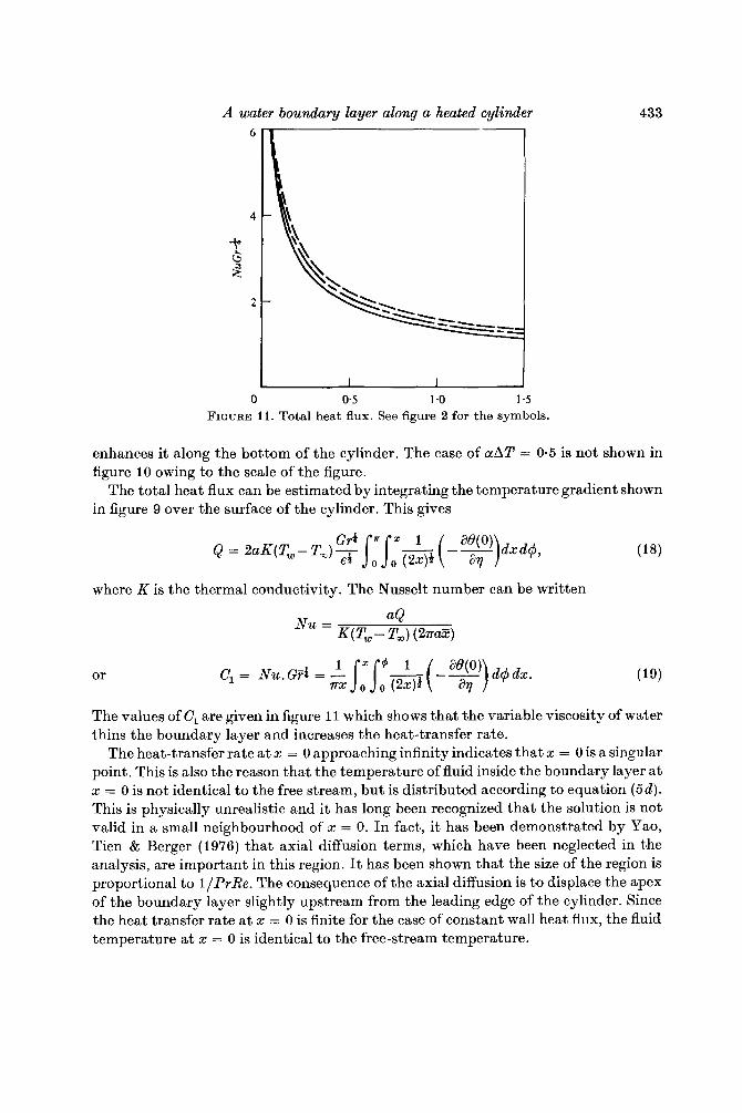
enhances i t along the bottom of the cylinder. The case of aAl’ = 0.5 is not shown in figure I0 owing to the scale of the figure.

The total heat flux can be estimated by integrating the temperature gradient shown in figure 9 over the surface of the cylinder. This gives

where K is the thermal conductivity. The Nusselt number can be written

or

The values of C, are given in figure i 1 which shows that the variable viscosity of water thins the boundary layer and increases the heat-transfer rate.

The heat-transfer rate a t x = 0 approaching infinity indicates that x = 0 is a singular point. This is also the reason that the temperature of fluid inside the boundary layer at x = 0 is not identical to the free stream, but is distributed according to equation (5d) . This is physically unrealistic and it has long been recognized that the solution is not valid in a small neighbourhood of x = 0. In fact, it has been demonstrated by Yao, Tien & Berger (1976) that axial diffusion terms, which have been neglected in the analysis, are important in this region. It has been shown that the size of the region is proportional to l/PrRe. The consequence of the axial diffusion is to displace the apex of the boundary layer slightly upstream from the leading edge of the cylinder. Since the heat transfer rate a t x = 0 is finite for the case of constant wall heat flux, the fluid temperature a t x = 0 is identical to the free-stream temperature.


4.3. Comparison of two cases

A criterion needs to be defined before the comparison of the flow development and the heat-transfer rate for the constant wall temperature and the constant wall heat flux can be meaningful. A reasonable criterion can be obtained by comparing the two cases on the basis of equal total heat flux. It can be shown that

07 = C,(x) G9-t

if the total heat fluxes are equal for the two cases. Equation (20) can be rearranged to

Since the values of C,, given in figure 11, are always larger than unity when x < 1-5, equation (21) shows that e% > €4 under the condition of equal total heat flux. Equation (2) and (8) indicate the physical location, 5 of the constant wall heat flux is smaller than that of the constant walI temperature for a given dimensionless x. Similar principles can be applied to other independent or dependent variables when one wants to compare the corresponding quantities.

The results, presented above, clearly show that the buoyancy and the variable viscosity of water have substantial effects on the development of the longitudinal boundary layer over a heated horizontal cylinder. As long as the cylinder is not short, the axisymmetric forced-convection boundary-layer flow does not approximate the real physical phenomenon well. Since the boundary-layer development in the entry region of a heated horizontal pipe is similar to that of the boundary layer over a horizontal cylinder, these two effects are also important, and cannot be neglected in estimating the flow resistance and the heat-transfer rate in a heated pipe flow.

R E F E R E N C E S

BARKER, S. J. & JENNINGS, C. G. 1977 The effect of wall heating on transition in water bound-

DWYER, H. A. 1968 Solution of a three-dimensional boundary layer-flow with separation.

KELLER, H. B. 1975 Some computational problems in boundary-layer flows. Proc. 4th Int. Conf. on Numerical Methods in Fluid Dynamics (ed. R. D. Richtmyer), Lecture notes in Physics, vol. 35, pp. 1-21. Springer.

ary layers. AGARD Symp. on Laminar Turbulent Transition, Copenhagen, Denmark.

A.I.A.A. J . 6, 1336-1342.

SINQH, M. P. 1974 Entry flow in a curved pipe. J . Fluid Mech. 65, 517-539. SMITH, A. M. 0. & CLUTTER, D. W. 1963 Solution of the incompressible laminar boundary-layer

VAN DYKE, M. 1964 Perturbation Method in Fluid Mechanics. Academic Press. YAO, L. S. 1978a Entry flow in a heated straight tube. J . Fluid Mech. 88, 465-483. YAO, L. S. 1978b Free-forced convection in the entry region of a heated straight pipe. Trans.

YAO, L. S. & BEROER, S. A. 1975 Entry flow in a curved pipe. J . Fluid Mech. 67, 177-196. YAO, L. S. & CATTON, I. 1977 Buoyancy cross-flow effects in the longitudinal boundary layer

on a heated horizontal cylinder. Trans. A.S.M.E. C, J . Heat Transfer 99, 122-124. YAO, L. S. & CATTON, I. 1978 The effects of variable viscosity on buoyancy cross-flow on a

heated horizontal cylinder. Int . J . Heat Mass Transfer 21, 407-414. YAO, L. S., CATTON, I. & MCDONOUGH, J. M. 1978 Free-forced convection from a heated

longitudinal horizontal cylinder. Numerical Heat Transfer 1, 255-266. YAO, L. S., TIEN, C. L. & BEROER, 8. A. 1976 Thermal analysis of a fast moving slab in two

adjacent temperature chambers. Trans. A.S.M.E. C, J . Heat Transfer 98, 326-329.

equations. A.I.A.A. J . 1 , 2062-2071.

A.S.M.E. C, J . Heat Transfer 100, 212-219.

Buoyancy-driven asymmetric water boundary layer along a heated cylinder

Documents

Transcript of Buoyancy-driven asymmetric water boundary layer along a heated cylinder