DES5613.3d 8/17/2009 17:43:23

Desalination 248 (2009) 803–815

Horizontal round heated jets into calm uniform ambient

Spyros N. Michas, Panos N. Papanicolaou*

Hydromechanics and Environmental Engineering Laboratory, Department of Civil Engineering,University of Thessaly, Pedion Areos, 38334 Volos, Greece

email: panospap@uth.gr

Received 29 October 2008; accepted 1 December 2008

Abstract

In this article, we investigate horizontal, round, turbulent buoyant jets that discharge in a homogeneous calmambient fluid. In a series of experiments performed, the initial jet Richardson numbers ranged from very small(jet-like) to around unity (plume-like), to include the full extent of applications. The mixing characteristicssuch as trajectories obtained with video imaging, turbulence properties measured with fast response thermistors,and dilution factors are evaluated. The trajectories of buoyancy-conserving horizontal jets bend faster than thoseobserved in heated jets. The flow resembles a jet-like behavior in the ‘horizontal’ regime, while the mean andturbulent temperature profiles become asymmetrical in the transition and the ‘vertical’ regime. The maximumintensity of turbulence doubles in the ‘vertical’ regime if compared to that in the ‘horizontal’ part of the flow.Minimum dilutions obtained from experiments at the jet axis are compared to the results of a one-dimensionalnumerical model of a heated horizontal jet, where the loss of buoyancy flux has been accounted for.

Keywords: Horizontal; Buoyant jet; Heated; Uniform ambient; Turbulence measurements; Trajectory

1. Introduction

Liquid wastes such as hot water from coolingof thermal energy power plants, as well as theeffluent from wastewater treatment plants, areusually disposed by means of submerged out-falls in the coast near the plant site. Heavier salt-water from desalination plants can alsobe discharged from a floating pipeline, at the

surface of the receptor. The regulations regard-ing disposal of thermal or denser dischargesinto coastal waters are related to the volumetricdischarge rate and the subsequent dilution of thewastewater. Thus, the local seasonal temperatureand salinity of coastal waters must not exceedspecific values (usually 2–48C or 2–3 g/L). Theinitial dilution of the wastes obtained whenthey reach the free surface or the bottom of thereceptor is crucial with respect to the environ-mental effects of the effluent in the vicinity ofthe discharge area. For a specific receptordepth, use of horizontal jets results in longer

*Corresponding author.Presented at the Conference on Protection andRestoration of the Environment IX, KefaloniaGreece, June 30–July 3, 2008

0011-9164/09/$– See front matter © 2009 Published by Elsevier B.V.doi:10.1016/j.desal.2008.12.042

DES5613.3d 8/17/2009 17:43:23

trajectories and subsequently in entrainment andmixing of greater amounts of ambient fluid, ifcompared to outfalls with vertical risers. Despitethe fact that horizontal jets are currently in useworldwide, so far little research has been carriedout to study their properties, although a greatnumber of experiments on vertical buoyant jetshave been reported [1–5]. Moreover, the majorityof research on horizontal buoyant jets [6–8] isbasically focused on the trajectory rather thanon the turbulence properties of the flow. Modelingof horizontal jets is usually implemented assum-ing that their cross-section normal to the axis iscircular [6, 9–11]. Also, the flow parameters(model ‘constants’) used such as the entrainmentcoefficient ae and the spreading ratio l of the con-centration to the velocity profile are usually thosemeasured in vertical buoyant jets.

In this article, a set of experiments per-formed is employed to investigate round turbu-lent buoyant jets that discharge horizontally in amotionless, uniform, deep body of water. Thescope of the present investigation is to evaluatetheir turbulence and mixing characteristics,such as their trajectory and distributions of thetime-averaged excess temperature and turbu-lence intensity. Subsequently, the measureddilutions will be compared to the results from

a one-dimensional numerical model of a heatedhorizontal jet.

1.1. Theoretical background

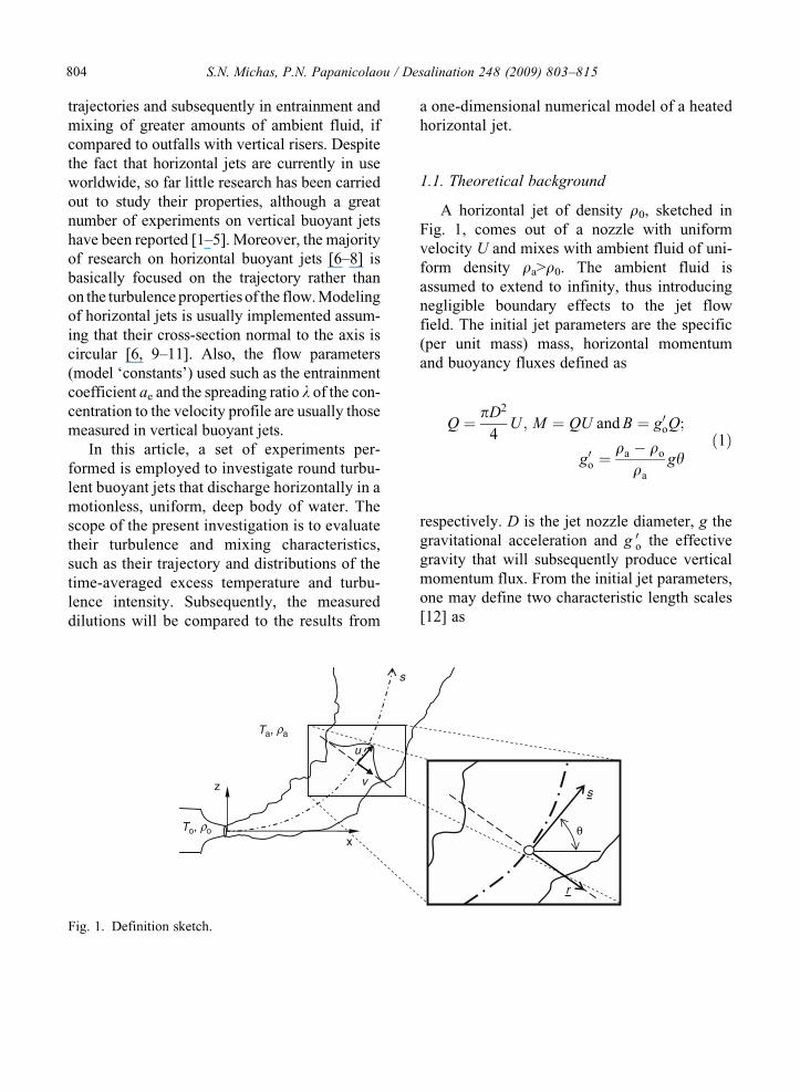
A horizontal jet of density r0, sketched inFig. 1, comes out of a nozzle with uniformvelocity U and mixes with ambient fluid of uni-form density ra>r0. The ambient fluid isassumed to extend to infinity, thus introducingnegligible boundary effects to the jet flowfield. The initial jet parameters are the specific(per unit mass) mass, horizontal momentumand buoyancy fluxes defined as

Q ¼ pD2

4U ; M ¼ QU and B ¼ g0oQ;

g0o ¼ra � ro

ra

gyð1Þ

respectively. D is the jet nozzle diameter, g thegravitational acceleration and g 0o the effectivegravity that will subsequently produce verticalmomentum flux. From the initial jet parameters,one may define two characteristic length scales[12] as

θ

r

s

s

x

z v

Ta, a

To, o

u

Fig. 1. Definition sketch.

S.N. Michas, P.N. Papanicolaou / Desalination 248 (2009) 803–815804

DES5613.3d 8/17/2009 17:43:23

lQ ¼Q

M1=2and lM ¼

M3=4

B1=2; ð2Þ

the ratio of which is defined to be the initial jetRichardson number Ro

Ro ¼lQ

lM¼ p

4

� �1=4

ffiffiffiffiffiffiffiffig0oD

pU¼ p

4

� �1=4

F�1o : ð3Þ

Fo is the initial densimetric Froude number ofthe jet. The density difference between jet andambient fluid may be due to the relative temper-ature or salinity of the two fluids. In a heated jet,temperature differences produce the densitydeficiency that is responsible for the initial jetspecific buoyancy flux. The initial jet heat fluxY = Q(To–Ta), where To is the jet temperatureand Ta the uniform ambient fluid temperature,is conserved. The dilution S at a point of thejet flow field is defined to be the ratio of the ini-tial temperature difference between jet andambient fluid, to the local time-averaged excess(above ambient) temperature

S ¼ To � Ta

T � Ta

: ð4Þ

The normalized jet trajectory [11] can beplotted as z/lM versus x/lM, x and z being the hor-izontal and vertical distances from the nozzle, ofa point located on the jet axis. The normalizeddilution Sc along the axis

Sc

Fo¼ 1

Fo

To � Ta

T c � Ta

ð5Þ

is a function of the normalized elevation z/lM, T c

being the (maximum) time-averaged excesstemperature.

The local, over a jet cross-section A normal tothe axis as shown in Fig. 1, volume flux m(s),momentum m(s) and buoyancy b(s) specificfluxes due to the mean flow are

mðsÞ ¼Z

A

uðr; sÞdA ð6Þ

mðsÞ ¼Z

A

u2ðr; sÞdA ð7Þ

bðsÞ ¼Z

A

gra � rðr; sÞ

rauðr; sÞdA ð8Þ

respectively. Coordinates s and r are the distancealong the axis from the nozzle and the radial dis-tance from the jet axis, respectively. Assumingthat distributions of the time-averaged velocityu(r,s) that is parallel to the axis and the densitydeficiency Dr(r,s) are Gaussian, and also thatthe jet cross-section is circular, the integratedover the cross-section time-averaged equationsof motion can be written as [6, 10, 13]

dmds¼ 2

ffiffiffiffiffiffi2pp

aem1=2 ð9Þ

dm

ds¼ 1þ l2

2

mbm

sin y ð10Þ

dyds¼ 1þ l2

2

mbm2

cos y ð11Þ

dbds¼ 0 ð12Þ

where ae is the local entrainment coefficientproposed by Morton et al. [1], l = be/bu is theratio of density deficiency width over velocitywidth, and y is the angle between the jet axisand horizontal. Two more equations needed todetermine the jet trajectory are

dx

ds¼ cos y ð13Þ

S.N. Michas, P.N. Papanicolaou / Desalination 248 (2009) 803–815 805

DES5613.3d 8/17/2009 17:43:23

and

dz

ds¼ sin y ð14Þ

The system of six nonlinear differential equa-tions is an initial value problem, and it can besolved numerically (using for example a Runge-Kutta routine), once the entrainment coefficientae and the jet width ratio l are estimated properly.

2. Experiments

Experiments were performed in a transparentorthogonal tank with dimensions 1.00 m �0.80 m and 0.70 m deep, equipped with a periph-eral overflow to remove excess water. A set ofthree circular jet nozzles of diameters 5, 10and 15 mm could be mounted to the properlydesigned end of a 20 cm long, hollow PVC cyl-inder (plenum) of internal diameter 4 cm, with a7 cm long honeycomb section positioned at mid-length. The insulated against heat loss water sup-ply pipe was mounted on the other end of thePVC cylinder, in line with a PT100 temperaturesensor for recording of the jet fluid temperature.The horizontal jet plenum was supported on theshort side transparent tank wall with a specialmount that did not allow any leaks from themotionless tank fluid. It was positioned 10 cmbelow the free surface for the heavier saltwaterjets, or 10 cm above the tank bottom for thehot water jets, ensuring that the tank boundarieshad minimal effects on the flow. A water heater

served as constant head tank since it waspressurized with air at 2 atm, and a pressure-reducing valve installed in line maintained con-stant head conditions throughout the experiment.For the saltwater jet experiments, the waterheater has only served as a pressurized constanthead tank. The jet flow rate at the nozzle wasmeasured using a simple, ball-type flowmetersthat allowed the precise setting and control ofthe desired discharge.

The experimental procedure was similar forboth thermal and saltwater jets. For the saltwaterjets, the solution was initially prepared in a sep-arate tank and when ready it was transferred tothe pressurized tank. For the heated buoyantjets, a bypass pipe located upstream of the inletto the jet plenum was used to dispose someamount of hot water before each experimentuntil the temperature sensor PT100 displayedconstant water temperature. Then the hot waterwas let to fill the jet plenum and measurementswere taken after about 1 min, the time that wasnecessary for establishment of steady-state. Dur-ing the experiment, a series of still photographsand video were taken simultaneously to be usedfor the subsequent trajectory analysis.

An adequate number of experiments [14] inthe full range of initial jet Richardson numbersfrom 0.02 to about 1 (corresponding to asymp-totically pure jets and plumes respectively) wasexecuted, for Reynolds numbers from 660 to13,000. The range of the initial conditions ofthe flow is shown in Table 1. Jet trajectories

Table 1

Range of the initial conditions for the saltwater and heated jet experiments

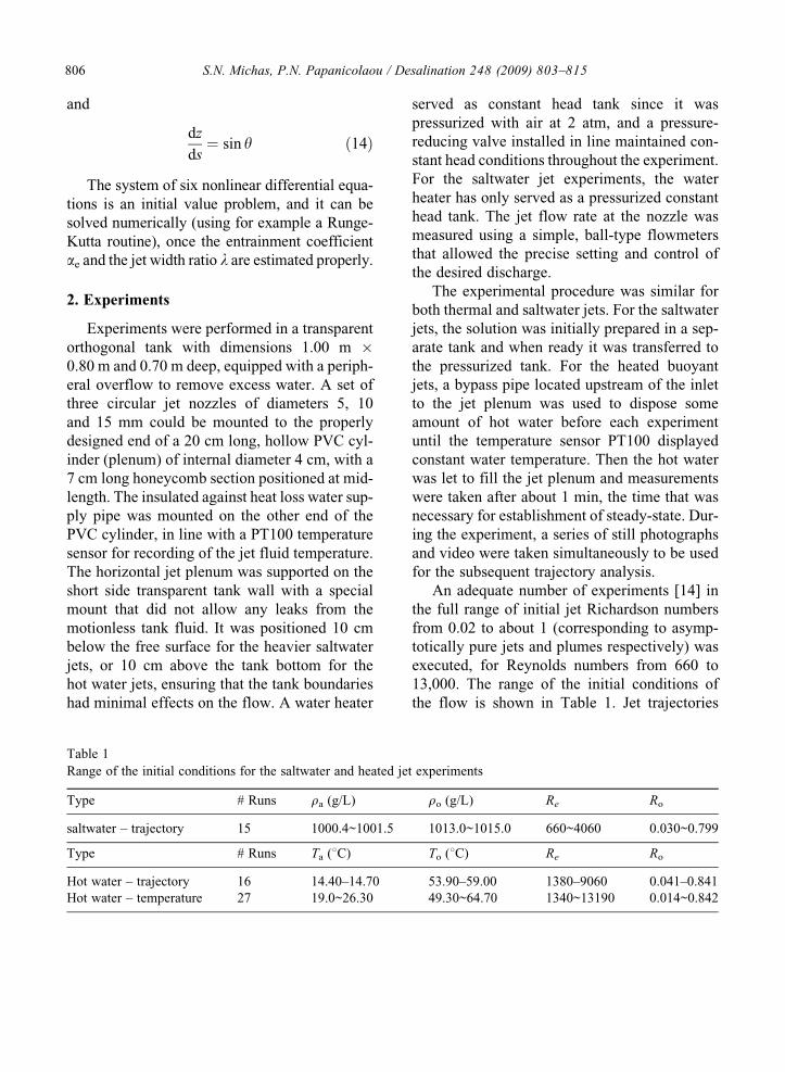
Type # Runs ra (g/L) ro (g/L) Re Ro

saltwater – trajectory 15 1000.4~1001.5 1013.0~1015.0 660~4060 0.030~0.799

Type # Runs Ta (8C) To (8C) Re Ro

Hot water – trajectory 16 14.40–14.70 53.90–59.00 1380–9060 0.041–0.841Hot water – temperature 27 19.0~26.30 49.30~64.70 1340~13190 0.014~0.842

S.N. Michas, P.N. Papanicolaou / Desalination 248 (2009) 803–815806

DES5613.3d 8/17/2009 17:43:23

were determined from shadowgraph videosusing a double grid based technique to minimizethe error in the measurement of the linear jetcharacteristics. Two series of jet images wereobtained, the first using saltwater jets into calmhomogeneous freshwater (buoyancy preserving)and the second using hot water jets into uniformcalm cold water ambient (buoyancy is a functionof the dilution). The photographs were correctedfor optical errors and subsequently the jet center-line coordinates were evaluated, from which thenormalized trajectories were determined.

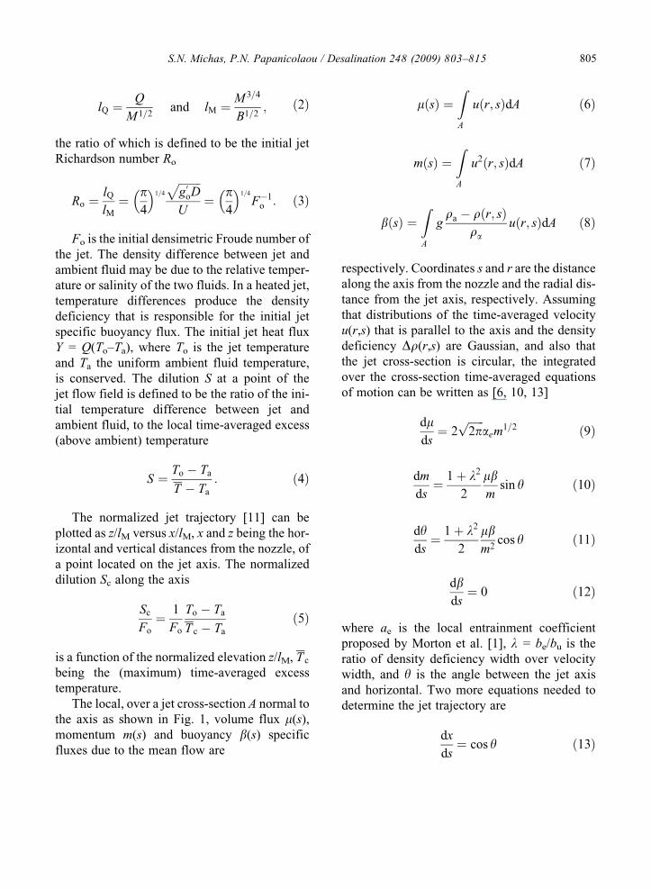
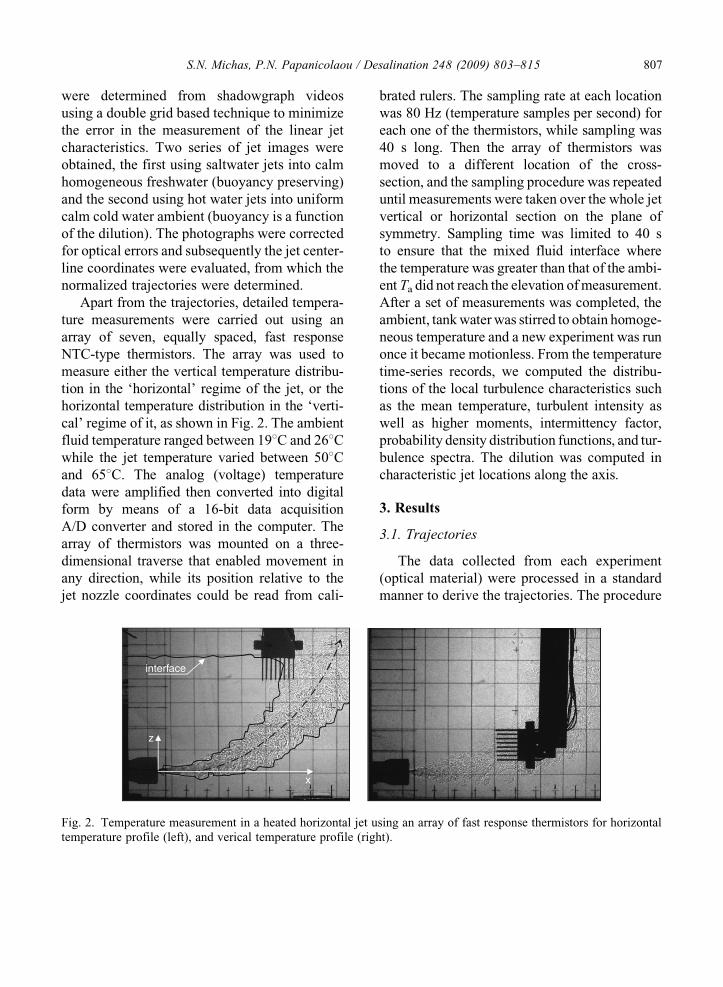
Apart from the trajectories, detailed tempera-ture measurements were carried out using anarray of seven, equally spaced, fast responseNTC-type thermistors. The array was used tomeasure either the vertical temperature distribu-tion in the ‘horizontal’ regime of the jet, or thehorizontal temperature distribution in the ‘verti-cal’ regime of it, as shown in Fig. 2. The ambientfluid temperature ranged between 198C and 268Cwhile the jet temperature varied between 508Cand 658C. The analog (voltage) temperaturedata were amplified then converted into digitalform by means of a 16-bit data acquisitionA/D converter and stored in the computer. Thearray of thermistors was mounted on a three-dimensional traverse that enabled movement inany direction, while its position relative to thejet nozzle coordinates could be read from cali-

brated rulers. The sampling rate at each locationwas 80 Hz (temperature samples per second) foreach one of the thermistors, while sampling was40 s long. Then the array of thermistors wasmoved to a different location of the cross-section, and the sampling procedure was repeateduntil measurements were taken over the whole jetvertical or horizontal section on the plane ofsymmetry. Sampling time was limited to 40 sto ensure that the mixed fluid interface wherethe temperature was greater than that of the ambi-ent Ta did not reach the elevation of measurement.After a set of measurements was completed, theambient, tank water was stirred to obtain homoge-neous temperature and a new experiment was runonce it became motionless. From the temperaturetime-series records, we computed the distribu-tions of the local turbulence characteristics suchas the mean temperature, turbulent intensity aswell as higher moments, intermittency factor,probability density distribution functions, and tur-bulence spectra. The dilution was computed incharacteristic jet locations along the axis.

3. Results

3.1. Trajectories

The data collected from each experiment(optical material) were processed in a standardmanner to derive the trajectories. The procedure

z

x

interface

Fig. 2. Temperature measurement in a heated horizontal jet using an array of fast response thermistors for horizontaltemperature profile (left), and verical temperature profile (right).

S.N. Michas, P.N. Papanicolaou / Desalination 248 (2009) 803–815 807

DES5613.3d 8/17/2009 17:43:23

included removal of color, adjustment of thegrayscale-level distribution to enhance the jetcontrast, rotation, layer alignment, perspectivecorrection, and barrel distortion removal (onlywhen necessary). Subsequently, the correctedphotographs were inserted in vector CAD soft-ware, where they were properly scaled to thedimensions of the jet midplane (of symmetry).Then the jet visual boundaries defined in everyset of photographs for each experiment weresuperimposed, and an average boundary wasdrawn on each side. Using a simple in-housebuilt algorithm, the jet-axis trajectory was deter-mined as the mid-distance from the average visualboundaries. Additionally, the video recordingshelped to refine the process, by improving theselection of the visual boundaries. The jet tra-jectories obtained were normalized using thecharacteristic length scale lM. The proceduredescribed above was applied to describe the tra-jectory in both thermal and saltwater jets.

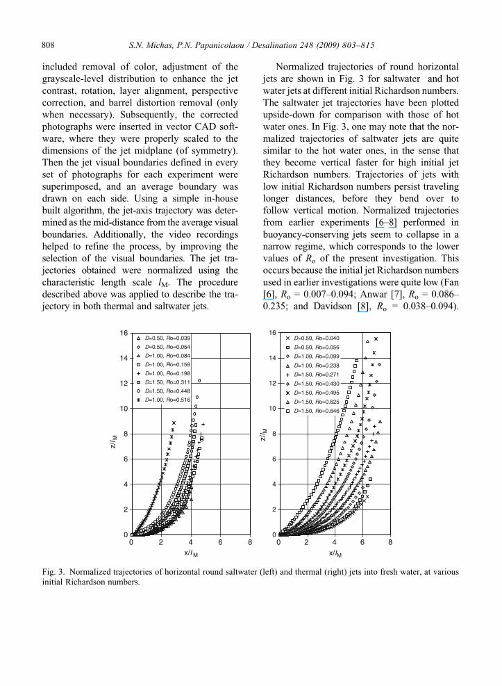
Normalized trajectories of round horizontaljets are shown in Fig. 3 for saltwater and hotwater jets at different initial Richardson numbers.The saltwater jet trajectories have been plottedupside-down for comparison with those of hotwater ones. In Fig. 3, one may note that the nor-malized trajectories of saltwater jets are quitesimilar to the hot water ones, in the sense thatthey become vertical faster for high initial jetRichardson numbers. Trajectories of jets withlow initial Richardson numbers persist travelinglonger distances, before they bend over tofollow vertical motion. Normalized trajectoriesfrom earlier experiments [6–8] performed inbuoyancy-conserving jets seem to collapse in anarrow regime, which corresponds to the lowervalues of Ro of the present investigation. Thisoccurs because the initial jet Richardson numbersused in earlier investigations were quite low (Fan[6], Ro = 0.007–0.094; Anwar [7], Ro = 0.086–0.235; and Davidson [8], Ro = 0.038–0.094).

0

2

4

6

8

10

12

14

16

z/l M

x/l M x/l M

z/l M

D=0.50, Ro=0.039

D=0.50, Ro=0.054

D=1.00, Ro=0.084

D=1.00, Ro=0.159

D=1.00, Ro=0.198

D=1.50, Ro=0.311

D=1.50, Ro=0.448

D=1.00, Ro=0.516

0

2

4

6

8

10

12

14

16

0 2 4 6 8 0 2 4 6 8

D=0.50, Ro=0.040

D=0.50, Ro=0.056

D=1.00, Ro=0.099

D=1.00, Ro=0.238

D=1.50, Ro=0.271

D=1.50, Ro=0.430

D=1.50, Ro=0.495

D=1.50, Ro=0.625

D=1.50, Ro=0.846

Fig. 3. Normalized trajectories of horizontal round saltwater (left) and thermal (right) jets into fresh water, at variousinitial Richardson numbers.

S.N. Michas, P.N. Papanicolaou / Desalination 248 (2009) 803–815808

DES5613.3d 8/17/2009 17:43:23

To our knowledge, there are no data availableregarding trajectories of horizontal heated jets.

One major difference in the trajectories ofheated jets if compared to those of saltwaterjets (with similar kinematic and buoyancy char-acteristics) is that the former are longer. Thismeans that a heated jet travels longer horizontaldistances x/lM than a saltwater one, to reach acertain elevation z/lM. This was expectedbecause hot water jets do not maintain their ini-tial buoyancy flux due to the variation of thethermal expansion coefficient of water with tem-perature. Once the warmer jet fluid mixes withcold ambient water its temperature is reduced,and so is the volume expansion coefficient.Therefore the initial jet specific buoyancy fluxis reduced, resulting gradually in lower verticalmomentum flux along the jet trajectory, if com-pared to that of the buoyancy-conserving salt-water jets. Reduction in vertical momentumresults in trajectories with longer horizontalcoordinates for the same vertical elevation ofthe buoyant jet axis.

In both saltwater and hot water jets, one mayclearly note that some trajectories start at anangle rather than initially being horizontal.This occurred at relatively high initial

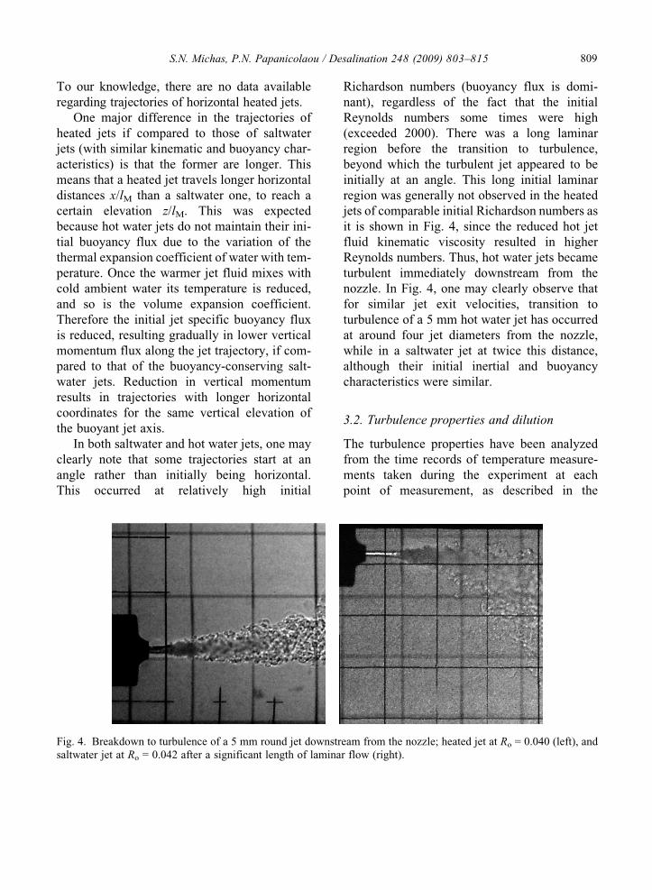
Richardson numbers (buoyancy flux is domi-nant), regardless of the fact that the initialReynolds numbers some times were high(exceeded 2000). There was a long laminarregion before the transition to turbulence,beyond which the turbulent jet appeared to beinitially at an angle. This long initial laminarregion was generally not observed in the heatedjets of comparable initial Richardson numbers asit is shown in Fig. 4, since the reduced hot jetfluid kinematic viscosity resulted in higherReynolds numbers. Thus, hot water jets becameturbulent immediately downstream from thenozzle. In Fig. 4, one may clearly observe thatfor similar jet exit velocities, transition toturbulence of a 5 mm hot water jet has occurredat around four jet diameters from the nozzle,while in a saltwater jet at twice this distance,although their initial inertial and buoyancycharacteristics were similar.

3.2. Turbulence properties and dilution

The turbulence properties have been analyzedfrom the time records of temperature measure-ments taken during the experiment at eachpoint of measurement, as described in the

Fig. 4. Breakdown to turbulence of a 5 mm round jet downstream from the nozzle; heated jet at Ro = 0.040 (left), andsaltwater jet at Ro = 0.042 after a significant length of laminar flow (right).

S.N. Michas, P.N. Papanicolaou / Desalination 248 (2009) 803–815 809

DES5613.3d 8/17/2009 17:43:24

previous chapter. The first four moments of thetemperature time series were computed. Fromthe time-averaged (mean) excess (above ambi-ent) temperature profiles, we computed the jetwidth be, that is the radial distance from theaxis (point with the highest mean temperature)where the mean excess temperature is 1/e(e being the base of Neperian logarithms)times that at the axis by fitting a Gaussiancurve to the data. The Gaussian was primarilyfit to the data corresponding to the outer jetboundary. The secondary plume of hot chunksof slowly rising to the surface fluid, observedin the inner jet boundary, affected the symmetryof time-averaged temperature distribution. Thenormalized time-averaged excess temperatureand turbulence intensity profiles can be plottedversus the normalized distance from the jetaxis with width be. Alternatively, the statisticalvalues can be normalized by the distance s ofthe measurement cross-section from the jet

origin. Apart from the abovementioned moments,other statistical values can be computed, namelyminimum and maximum values, hot/cold inter-face frequencies and intermittency factors.

In a horizontal turbulent buoyant jet, we havenoted three separate flow regimes. The one closeto the jet nozzle, characterized as the ‘horizon-tal’ part of the trajectory, is limited to the nor-malized distance x/lM<1.50, where the flow isessentially driven by the initial horizontal jetmomentum (jet-like). The flow regime wherez/lM>1.50 can be characterized as the bent overregime of the flow (mainly for buoyant jetswith low Ro), that is the result of the buoyancyforce acting on the jet (plume-like). The regimein between (1.50<x/lM<5) is a transition fromjet-like to plume-like flow.

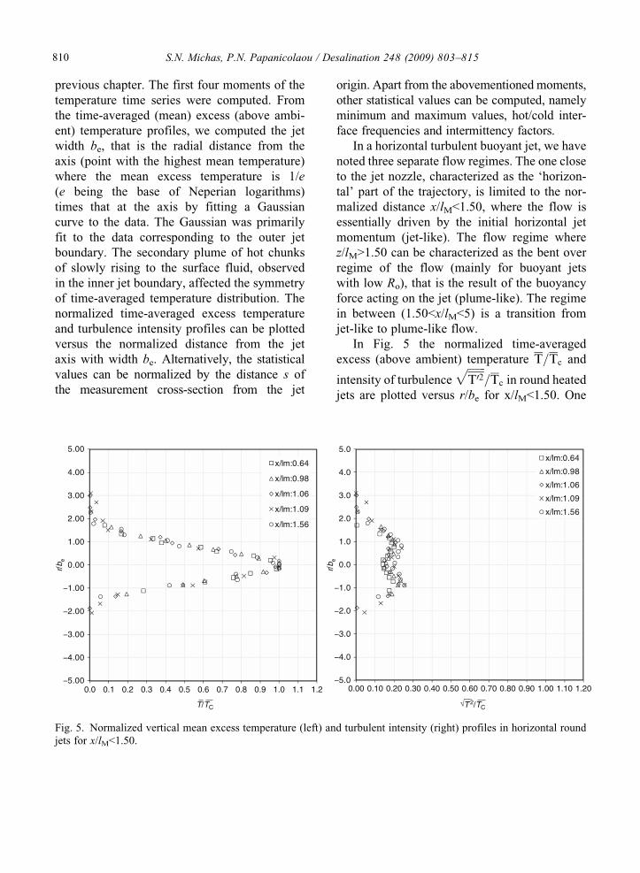
In Fig. 5 the normalized time-averagedexcess (above ambient) temperature T=Tc and

intensity of turbulenceffiffiffiffiffiffiffiT02

p=Tc in round heated

jets are plotted versus r/be for x/lM<1.50. One

−5.00

−4.00

−3.00

−2.00

−1.00

0.00

1.00

2.00

3.00

4.00

5.00

0.0 0.1 0.2 0.3 0.4 0.5 0.6 0.7 0.8 0.9 1.0 1.1 1.2

r/b e

r/b e

x/lm:0.64

x/lm:0.98

x/lm:1.06

x/lm:1.09

x/lm:1.56

−5.0

−4.0

−3.0

−2.0

−1.0

0.0

1.0

2.0

3.0

4.0

5.0

0.00 0.10 0.20 0.30 0.40 0.50 0.60 0.70 0.80 0.90 1.00 1.10 1.20

x/lm:0.64

x/lm:0.98

x/lm:1.06

x/lm:1.09

x/lm:1.56

T/TC T 2/TC√

Fig. 5. Normalized vertical mean excess temperature (left) and turbulent intensity (right) profiles in horizontal roundjets for x/lM<1.50.

S.N. Michas, P.N. Papanicolaou / Desalination 248 (2009) 803–815810

DES5613.3d 8/17/2009 17:43:24

may clearly note that both mean and turbulenttemperature profiles are symmetrical withrespect to r/be, while a double peak is apparentin the second one around r/be = 1. The profilesare very similar to those reported earlier [3] forround vertical heated jets. Therefore, the flowcan be characterized as jet-like when x/lM<1.50,as in the vertical heated jets.

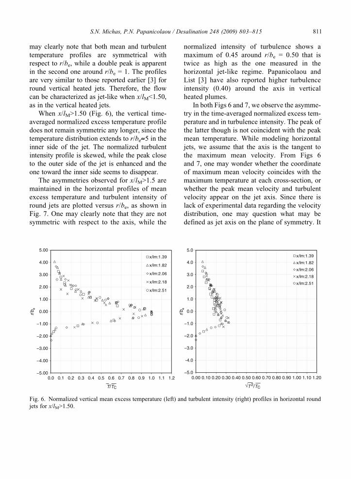
When x/lM>1.50 (Fig. 6), the vertical time-averaged normalized excess temperature profiledoes not remain symmetric any longer, since thetemperature distribution extends to r/be»5 in theinner side of the jet. The normalized turbulentintensity profile is skewed, while the peak closeto the outer side of the jet is enhanced and theone toward the inner side seems to disappear.

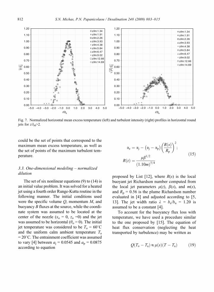
The asymmetries observed for x/lM>1.5 aremaintained in the horizontal profiles of meanexcess temperature and turbulent intensity ofround jets are plotted versus r/be, as shown inFig. 7. One may clearly note that they are notsymmetric with respect to the axis, while the

normalized intensity of turbulence shows amaximum of 0.45 around r/be = 0.50 that istwice as high as the one measured in thehorizontal jet-like regime. Papanicolaou andList [3] have also reported higher turbulenceintensity (0.40) around the axis in verticalheated plumes.

In both Figs 6 and 7, we observe the asymme-try in the time-averaged normalized excess tem-perature and in turbulence intensity. The peak ofthe latter though is not coincident with the peakmean temperature. While modeling horizontaljets, we assume that the axis is the tangent tothe maximum mean velocity. From Figs 6and 7, one may wonder whether the coordinateof maximum mean velocity coincides with themaximum temperature at each cross-section, orwhether the peak mean velocity and turbulentvelocity appear on the jet axis. Since there islack of experimental data regarding the velocitydistribution, one may question what may bedefined as jet axis on the plane of symmetry. It

−5.00

−4.00

−3.00

−2.00

−1.00

0.00

1.00

2.00

3.00

4.00

5.00

x/lm:1.39

x/lm:1.82

x/lm:2.06

x/lm:2.18

x/lm:2.51

−5.0

-4.0

−3.0

−2.0

−1.0

0.0

1.0

2.0

3.0

4.0

5.0x/lm:1.39

x/lm:1.82

x/lm:2.06

x/lm:2.18

x/lm:2.51

0.0 0.1 0.2 0.3 0.4 0.5 0.6 0.7 0.8 0.9 1.0 1.1 1.2 0.00 0.10 0.20 0.30 0.40 0.50 0.60 0.70 0.80 0.90 1.00 1.10 1.20

T/TC T 2/TC√

r/b e

r/b e

Fig. 6. Normalized vertical mean excess temperature (left) and turbulent intensity (right) profiles in horizontal roundjets for x/lM>1.50.

S.N. Michas, P.N. Papanicolaou / Desalination 248 (2009) 803–815 811

DES5613.3d 8/17/2009 17:43:24

could be the set of points that correspond to themaximum mean excess temperature, as well asthe set of points of the maximum turbulent tem-perature.

3.3. One-dimensional modeling – normalizeddilution

The set of six nonlinear equations (9) to (14) isan initial value problem. It was solved for a heatedjet using a fourth order Runge-Kutta routine in thefollowing manner. The initial conditions usedwere the specific volume Q, momentum M, andbuoyancy B fluxes at the source, while the coordi-nate system was assumed to be located at thecenter of the nozzle (xo = 0, zo =0) and the jetwas assumed to be horizontal (yo = 0). The initialjet temperature was considered to be To = 608Cand the uniform calm ambient temperature Ta

= 208C. The entrainment coefficient was assumedto vary [4] between aj = 0.0545 and ap = 0.0875according to equation

ae ¼ aj � aj � ap

� � RðsÞRp

� �2

;

RðzÞ ¼ mb1=2

1:10mð Þ5=4

ð15Þ

proposed by List [12], where R(s) is the localbuoyant jet Richardson number computed fromthe local jet parameters m(z), b(s), and m(s),and Rp = 0.56 is the plume Richardson numberevaluated in [4] and adjusted according to [5,13]. The jet width ratio l = be/bu = 1.20 isassumed to be a constant [4].

To account for the buoyancy flux loss withtemperature, we have used a procedure similarto the one proposed by [15]. The equation ofheat flux conservation (neglecting the heattransported by turbulence) may be written as

QðTo � TaÞ&mðsÞ T � Tað Þ ð19Þ

0.00

0.10

0.20

0.30

0.40

0.50

0.60

0.70

0.80

0.90

1.00

1.10

1.20z/lm:1.34z/lm:1.91z/lm:2.26z/lm:3.93z/lm:4.38z/lm:5.84z/lm:6.47z/lm:9.02z/lm:12.66z/lm:14.69

0.00

0.10

0.20

0.30

0.40

0.50

0.60

0.70

0.80

0.90

1.00

1.10

1.20

−5.0 −4.0 −3.0 −2.0 −1.0 0.0 1.0 2.0 3.0 4.0 5.0 −5.0 −4.0 −3.0 −2.0 −1.0 0.0 1.0 2.0 3.0 4.0 5.0

z/lm:1.34z/lm:1.91z/lm:2.26z/lm:3.93z/lm:4.38z/lm:5.84z/lm:6.47z/lm:9.02z/lm:12.66z/lm:14.69

T/T

C

T2 /

TC

√r/be r/be

Fig. 7. Normalized horizontal mean excess temperature (left) and turbulent intensity (right) profiles in horizontal roundjets for z/lM>2.

S.N. Michas, P.N. Papanicolaou / Desalination 248 (2009) 803–815812

DES5613.3d 8/17/2009 17:43:24

where T is the average, over the jet cross-section temperature. Since an average overthe cross-section density can be expressed as afunction of the average temperaturerðsÞ ¼ f TðsÞð Þ, the local specific buoyancyflux at s+ds can be computed approximatelyfrom equation

bðsþ dsÞ&mðsÞ rðsÞ � ra

ro

g: ð20Þ

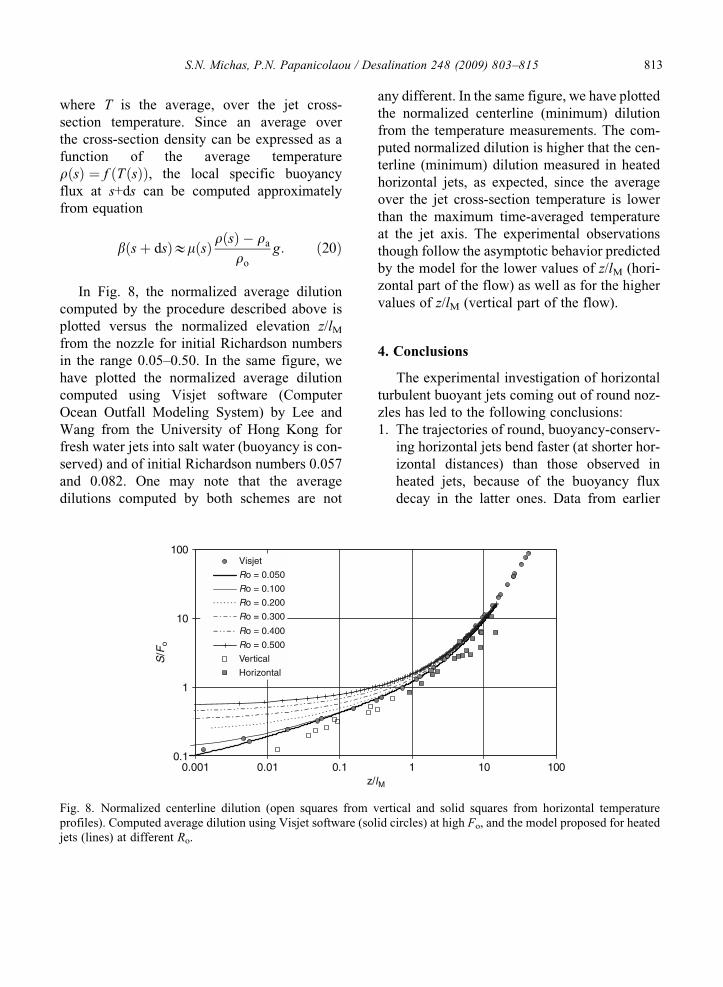
In Fig. 8, the normalized average dilutioncomputed by the procedure described above isplotted versus the normalized elevation z/lMfrom the nozzle for initial Richardson numbersin the range 0.05–0.50. In the same figure, wehave plotted the normalized average dilutioncomputed using Visjet software (ComputerOcean Outfall Modeling System) by Lee andWang from the University of Hong Kong forfresh water jets into salt water (buoyancy is con-served) and of initial Richardson numbers 0.057and 0.082. One may note that the averagedilutions computed by both schemes are not

any different. In the same figure, we have plottedthe normalized centerline (minimum) dilutionfrom the temperature measurements. The com-puted normalized dilution is higher that the cen-terline (minimum) dilution measured in heatedhorizontal jets, as expected, since the averageover the jet cross-section temperature is lowerthan the maximum time-averaged temperatureat the jet axis. The experimental observationsthough follow the asymptotic behavior predictedby the model for the lower values of z/lM (hori-zontal part of the flow) as well as for the highervalues of z/lM (vertical part of the flow).

4. Conclusions

The experimental investigation of horizontalturbulent buoyant jets coming out of round noz-zles has led to the following conclusions:1. The trajectories of round, buoyancy-conserv-

ing horizontal jets bend faster (at shorter hor-izontal distances) than those observed inheated jets, because of the buoyancy fluxdecay in the latter ones. Data from earlier

0.1

1

10

100

0.001 0.01 0.1 1 10 100z/lM

S/F

o

Visjet

Ro = 0.050

Ro = 0.100

Ro = 0.200

Ro = 0.300

Ro = 0.400

Ro = 0.500

Vertical

Horizontal

Fig. 8. Normalized centerline dilution (open squares from vertical and solid squares from horizontal temperatureprofiles). Computed average dilution using Visjet software (solid circles) at high Fo, and the model proposed for heatedjets (lines) at different Ro.

S.N. Michas, P.N. Papanicolaou / Desalination 248 (2009) 803–815 813

DES5613.3d 8/17/2009 17:43:24

experiments on buoyancy conserving jets arelimited to Ro<0.235, and congruent with thefindings of the present investigation.

2. The flow behaves as a simple jet (jet-like) inthe ‘horizontal’ part of the trajectory, namelyfor x/lM<1.50, where the horizontal momen-tum flux is dominant. The distributions ofthe mean excess and turbulent temperatureare symmetric with respect to the axis, similarto those reported for round vertical heated jets.

3. The flow is in transition from jets to plumeswhen 1<x/lM<5. It is practically consideredto be plume-like (vertical momentum flux isdominant) when x/lM>5 or z/lM>2. The distri-butions of the mean excess and turbulent tem-perature are not symmetric any longer, andthe two peaks characteristic of the turbulenttemperature in the jet-like regime coalesceinto a single one in the plume-like regime.The intensity of turbulence is doubled ifcompared to that in jets. The maximumintensity of turbulence appears off the jetaxis, around r/be = 0.50. This can raise aquestion regarding the definition of the jetaxis, which is usually considered to be thepoint of the jet section on the plane ofsymmetry, where the time-averaged excesstemperature is the highest.

4. The normalized measured (minimum) dilu-tion along the jet axis seems to follow thesame asymptotic power laws for low andhigh dimensionless elevations from the noz-zle, with the ones computed using commer-cial software and the one-dimensionalmodel of a heated jet presented in this article.As expected, the computed, average over thecross-section dilution is higher if comparedto that measured at the jet axis.

Acknowledgment

The present work was supported by the pro-gram ‘‘EPEAEK II – HERAKLEITOS’’ underGrant UTH 51808.07, jointly funded by the

European Social Fund and National Resources.The assistance of Mr. Demetris Karaberopoulos,Mr. Elias Pappas, and Mr. Manolis Lasithiotakisis gratefully appreciated.

Nomenclature

List of symbols

A jet cross-sectional areabu 1/e velocity width, lateral distance from axis

where u = 0.37uc

be 1/e temperature width, lateral distance fromaxis where T ¼ 0:37T c

B specific buoyancy flux at the sourceD jet diameterFo densimetric Froude number at the sourceg gravitational accelerationg0 effective gravitational accelerationlQ; lM characteristic length scalesM jet specific momentum flux at the sourcem local specific momentum flux at distance s along

jet axisQ specific mass (volume) flux at the sourceRo jet Richardson number at the sourceR(s) local jet Richardson numberRp asymptotic plume Richardson numberr coordinate perpendicular to the jet axisRe Reynolds number at the sources distance along the jet axis from the originS dilutionT average temperatureT time-averaged temperatureU jet exit velocityu time-averaged axial velocityv time-averaged radial velocityx, z coordinatesY heat flux at the source

Greek Symbols

ae entrainment coefficientaj jet entrainment coefficientap plume entrainment coefficientb local specific buoyancy flux at distance sy angle of jet axis at distance s with respect to

horizontall (= be/bu) temperature to velocity 1/e width

ratio

S.N. Michas, P.N. Papanicolaou / Desalination 248 (2009) 803–815814

DES5613.3d 8/17/2009 17:43:24

References

[1] B.R Morton, G.I. Taylor, and J.S. Turner. Proc.Roy. Soc. London, A 234 (1956) 1–23.

[2] N.E. Kotsovinos. A study of the entrainmentand turbulence in a plane buoyant jet, ReportNo. KH-R-32, California Institute of Technology,Pasadena, California, 1975.

[3] P.N. Papanicolaou and E.J. List. Int. J. Heat MassTransfer 30 (1987) 2057–2071.

[4] P.N. Papanicolaou and E.J. List. J. Fluid Mech.195 (1988) 341–391.

[5] H. Wang and A.W.-K. Law. J. Fluid Mech. 459(2002) 397–428.

[6] L.-N. Fan. Turbulent buoyant jets into stratified orflowing ambient fluids, Report No. KH-R-15,

W.M. Keck Laboratory of Hydraulics and WaterResources, California Institute of Technology,Pasadena, California, 1967.

[7] H.O. Anwar. Proc. ASCE, J. Hyd. Div. 95(4)(1969) 1289–1303.

[8] I.R. Wood, R.G. Bell, and D.L. Wilkinson. Oceandisposal of wastewater, Advanced Series on OceanEngineering, Vol. 8, 1993, p. 44, Figure 4.12, fromM.J. Davidson, 1988.

[9] G. Abraham. Proc. ASCE, J. Hyd. Div. 91(4)(1965) 138–154.

[10] L.-N. Fan and N.H. Brooks. Proc. ASCE, J. Hyd.Div. 92(2) (1966) 423–429.

[11] G.H. Jirka. Env. Fluid Mech. 4 (2004) 1–56.[12] H.B., Fischer, E.J. List, R.C.Y. Koh, J. Imberger,

and N.H. Brooks. Mixing in inland and coastalwaters, Academic Press, London, 1979.

[13] P.N. Papanicolaou, I.G. Papakonstantis, andG.C. Christodoulou. J. Fluid Mech. 614 (2008)447–470.

[14] S.N. Michas, Experimental investigation of hori-zontal round and non-axisymmetric buoyantjets in a uniform calm ambient, (In Greek), Ph.D.Thesis, Hydromechanics and Environmental Engi-neering Laboratory, Department of Civil Engineer-ing, University of Thessaly, 2008.

[15] P.N. Papanicolaou and T.J. Kokkalis. Int. J. HeatMass Trans. 51 (2008) 4109–4120.

m local specific mass flux or volume flux atdistance s along jet axis

r density

Superscripts and Subscripts

ð Þ0 deviation from a time averaged mean

ð Þ time-averaged valuesc centerline valueo initial values at jet origina values of the ambient fluid variables

S.N. Michas, P.N. Papanicolaou / Desalination 248 (2009) 803–815 815