A Two Dimensional Characteristic Galerkin Finite

Element Solution of Fluid Flow Over Heated

Cylinder

Shahzada Khurram

Department of Mathematics, Air University

September 26, 2013

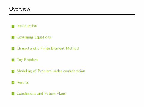
Overview

1 Introduction

2 Governing Equations

3 Characteristic Finite Element Method

4 Toy Problem

5 Modeling of Problem under consideration

6 Results

7 Conclusions and Future Plans

Introduction

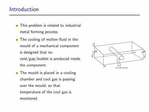
This problem is related to industrial

metal forming process.

The cooling of molten fluid in the

mould of a mechanical component

is designed that no

void/gap/bubble is produced inside

the component.

The mould is placed in a cooling

chamber and cool gas is passing

over the mould, so that

temperature of the cool gas is

monitored.

Air

in

Air

out

x

y

zHot solid cylinder

Introduction

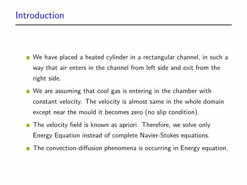
We have placed a heated cylinder in a rectangular channel, in such a

way that air enters in the channel from left side and exit from the

right side.

We are assuming that cool gas is entering in the chamber with

constant velocity. The velocity is almost same in the whole domain

except near the mould it becomes zero (no slip condition).

The velocity field is known as apriori. Therefore, we solve only

Energy Equation instead of complete Navier-Stokes equations.

The convection-diffusion phenomena is occurring in Energy equation.

Two Dimensional Domain (in dotted line)

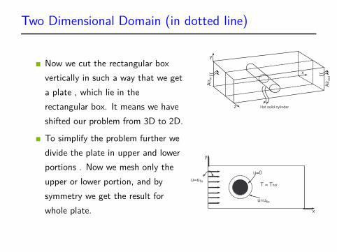
Now we cut the rectangular box

vertically in such a way that we get

a plate , which lie in the

rectangular box. It means we have

shifted our problem from 3D to 2D.

To simplify the problem further we

divide the plate in upper and lower

portions . Now we mesh only the

upper or lower portion, and by

symmetry we get the result for

whole plate.A

irin

Air

out

x

y

z Hot solid cylinder

x

y

u=0

u=ufix

T = Thot

u=ufix

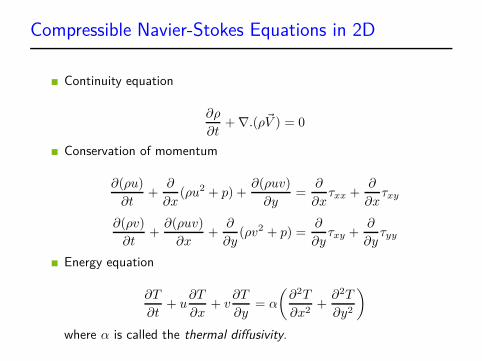
Compressible Navier-Stokes Equations in 2D

Continuity equation

∂ρ

∂t+ ∇.(ρ~V ) = 0

Conservation of momentum

∂(ρu)

∂t+

∂

∂x(ρu2 + p) +

∂(ρuv)

∂y=

∂

∂xτxx +

∂

∂xτxy

∂(ρv)

∂t+

∂(ρuv)

∂x+

∂

∂y(ρv2 + p) =

∂

∂yτxy +

∂

∂yτyy

Energy equation

∂T

∂t+ u

∂T

∂x+ v

∂T

∂y= α

(

∂2T

∂x2+

∂2T

∂y2

)

where α is called the thermal diffusivity.

Solution of Navier-Stokes Equations

The exact solution of Navier-Stoke’s Equation are rare because these non

linear partial differential equations. The exact solution is possible only in

some special cases for example Stoke’s 1st problem, Stoke’s 2nd problem,

Couettee flow, Poiseuille flow. So in order to solve complex flow problem,

we use computational techniques. There are many computational

techniques available, for example

Finite Difference Method (Grid Points)

Finite Volume Method (Cells/Control Volumes)

Finite Element Method (Elements)

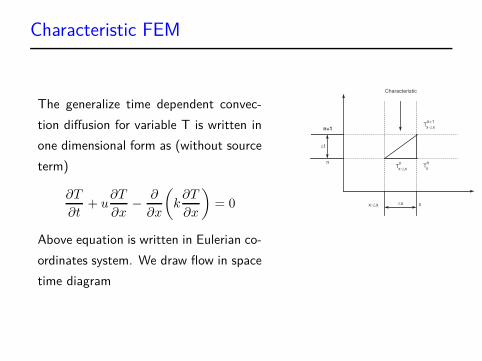
Characteristic FEM

The generalize time dependent convec-

tion diffusion for variable T is written in

one dimensional form as (without source

term)

∂T

∂t+ u

∂T

∂x−

∂

∂x

(

k∂T

∂x

)

= 0

Above equation is written in Eulerian co-

ordinates system. We draw flow in space

time diagram

n+1

∆t

∆xx-∆x x

nT

n

x-∆x

Tn+1

x-∆x

Tn

x

Characteristic

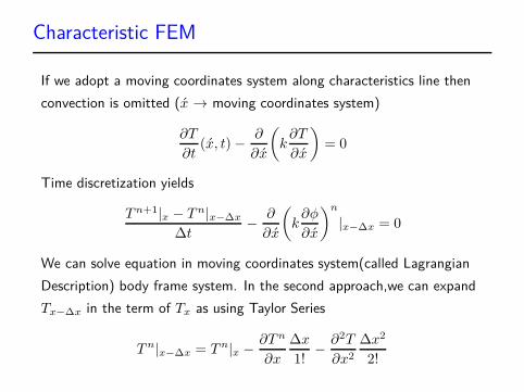
Characteristic FEM

If we adopt a moving coordinates system along characteristics line then

convection is omitted (x́ → moving coordinates system)

∂T

∂t(x́, t) −

∂

∂x́

(

k∂T

∂x́

)

= 0

Time discretization yields

T n+1|x − T n|x−∆x

∆t−

∂

∂x́

(

k∂φ

∂x́

)n

|x−∆x = 0

We can solve equation in moving coordinates system(called Lagrangian

Description) body frame system. In the second approach,we can expand

Tx−∆x in the term of Tx as using Taylor Series

T n|x−∆x = T n|x −∂T n

∂x

∆x

1!−

∂2T

∂x2

∆x2

2!

Characteristic FEM

Similarly, the diffusion term is expanded as

∂

∂x́

(

k∂T

∂x′

)

|x−∆x =∂

∂x

(

k∂T

∂x

)n

|x −∂

∂x

[

∂

∂x

(

k∂T

∂x

)n]

∆x

Neglecting higher order and substituting, we have

T n+1 − T n

∆t= −

∆x

∆t

∂T n

∂x+

∆x2

2∆t

∂2T n

∂x2+

∂

∂x

(

k∂T

∂x

)n

Substituting ∆x=u∆t, we get

T n+1 − T n

∆t= −u

∂T n

∂x+ u2 ∆t

2

∂2T n

∂x2+

∂

∂x

(

k∂T

∂x

)n

We notice that an additional diffusion type term has occurred. This term

usually control the overshooting in numerical solution by selecting P e > 1

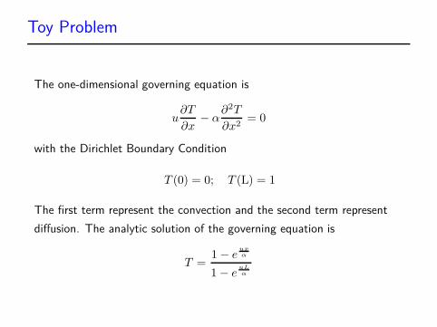
Toy Problem

The one-dimensional governing equation is

u∂T

∂x− α

∂2T

∂x2= 0

with the Dirichlet Boundary Condition

T (0) = 0; T (L) = 1

The first term represent the convection and the second term represent

diffusion. The analytic solution of the governing equation is

T =1 − e

ux

α

1 − euL

α

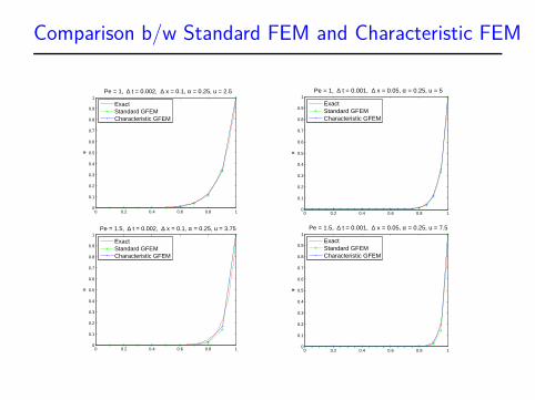
Comparison b/w Standard FEM and Characteristic FEM

0 0.2 0.4 0.6 0.8 10

0.1

0.2

0.3

0.4

0.5

0.6

0.7

0.8

0.9

1

φ

Pe = 1, ∆ t = 0.002, ∆ x = 0.1, α = 0.25, u = 2.5

ExactStandard GFEMCharacteristic GFEM

0 0.2 0.4 0.6 0.8 10

0.1

0.2

0.3

0.4

0.5

0.6

0.7

0.8

0.9

1

φ

Pe = 1, ∆ t = 0.001, ∆ x = 0.05, α = 0.25, u = 5

ExactStandard GFEMCharacteristic GFEM

0 0.2 0.4 0.6 0.8 10

0.1

0.2

0.3

0.4

0.5

0.6

0.7

0.8

0.9

1

φ

Pe = 1.5, ∆ t = 0.002, ∆ x = 0.1, α = 0.25, u = 3.75

ExactStandard GFEMCharacteristic GFEM

0 0.2 0.4 0.6 0.8 10

0.1

0.2

0.3

0.4

0.5

0.6

0.7

0.8

0.9

1

φ

Pe = 1.5, ∆ t = 0.001, ∆ x = 0.05, α = 0.25, u = 7.5

ExactStandard GFEMCharacteristic GFEM

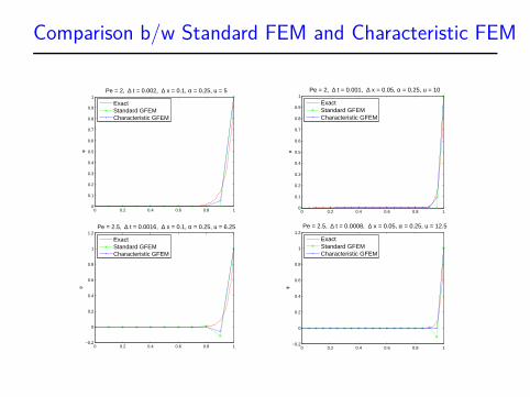
Comparison b/w Standard FEM and Characteristic FEM

0 0.2 0.4 0.6 0.8 10

0.1

0.2

0.3

0.4

0.5

0.6

0.7

0.8

0.9

1

φ

Pe = 2, ∆ t = 0.002, ∆ x = 0.1, α = 0.25, u = 5

ExactStandard GFEMCharacteristic GFEM

0 0.2 0.4 0.6 0.8 10

0.1

0.2

0.3

0.4

0.5

0.6

0.7

0.8

0.9

1

φ

Pe = 2, ∆ t = 0.001, ∆ x = 0.05, α = 0.25, u = 10

ExactStandard GFEMCharacteristic GFEM

0 0.2 0.4 0.6 0.8 1−0.2

0

0.2

0.4

0.6

0.8

1

1.2

φ

Pe = 2.5, ∆ t = 0.0016, ∆ x = 0.1, α = 0.25, u = 6.25

ExactStandard GFEMCharacteristic GFEM

0 0.2 0.4 0.6 0.8 1−0.2

0

0.2

0.4

0.6

0.8

1

1.2

φ

Pe = 2.5, ∆ t = 0.0008, ∆ x = 0.05, α = 0.25, u = 12.5

ExactStandard GFEMCharacteristic GFEM

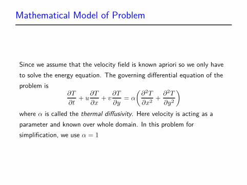
Mathematical Model of Problem

Since we assume that the velocity field is known apriori so we only have

to solve the energy equation. The governing differential equation of the

problem is∂T

∂t+ u

∂T

∂x+ v

∂T

∂y= α

(

∂2T

∂x2+

∂2T

∂y2

)

where α is called the thermal diffusivity. Here velocity is acting as a

parameter and known over whole domain. In this problem for

simplification, we use α = 1

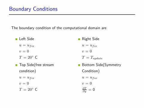
Boundary Conditions

The boundary condition of the computational domain are

Left Side

u = ufix

v = 0

T = 20◦ C

Top Side(free stream

condition)

u = ufix

v = 0

T = 20◦ C

Right Side

u = ufix

v = 0

T = Tupdate

Bottom Side(Symmetry

Condition)

u = ufix

v = 0∂T∂y

= 0

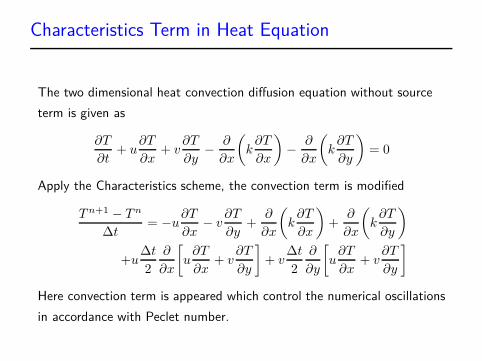
Characteristics Term in Heat Equation

The two dimensional heat convection diffusion equation without source

term is given as

∂T

∂t+ u

∂T

∂x+ v

∂T

∂y−

∂

∂x

(

k∂T

∂x

)

−∂

∂x

(

k∂T

∂y

)

= 0

Apply the Characteristics scheme, the convection term is modified

T n+1 − T n

∆t= −u

∂T

∂x− v

∂T

∂y+

∂

∂x

(

k∂T

∂x

)

+∂

∂x

(

k∂T

∂y

)

+u∆t

2

∂

∂x

[

u∂T

∂x+ v

∂T

∂y

]

+ v∆t

2

∂

∂y

[

u∂T

∂x+ v

∂T

∂y

]

Here convection term is appeared which control the numerical oscillations

in accordance with Peclet number.

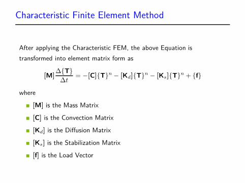
Characteristic Finite Element Method

After applying the Characteristic FEM, the above Equation is

transformed into element matrix form as

[M]∆{T}

∆t= −[C]{T}n − [Kd]{T}n − [Ks]{T}n + {f}

where

[M] is the Mass Matrix

[C] is the Convection Matrix

[Kd] is the Diffusion Matrix

[Ks] is the Stabilization Matrix

[f] is the Load Vector

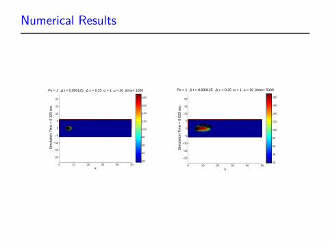
Numerical Results

0 10 20 30 40 50

−20

−15

−10

−5

0

5

10

15

20

x

Sim

ulat

ion

Tim

e =

0.1

25 s

ec

Pe = 1 ,∆ t = 0.000125 ,∆ x = 0.25 ,α = 1 ,u = 20 ,itime= 1000

20

40

60

80

100

120

140

160

180

0 10 20 30 40 50

−20

−15

−10

−5

0

5

10

15

20

29.8319941.17652

52.5210663.8655975.2101286.5546697.89919109.2437

x

Sim

ulat

ion

Tim

e =

0.6

25 s

ec

Pe = 1 ,∆ t = 0.000125 ,∆ x = 0.25 ,α = 1 ,u = 20 ,itime= 5000

20

40

60

80

100

120

140

160

180

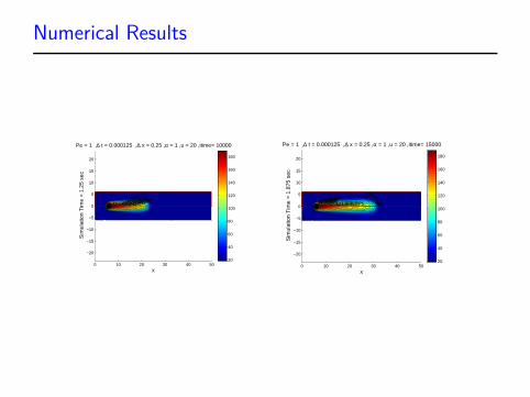
Numerical Results

0 10 20 30 40 50

−20

−15

−10

−5

0

5

10

15

20

29.8578741.2006852.5434963.8862975.229186.5719197.91472109.2575120.6003131.9431143.286154.6288

x

Sim

ulat

ion

Tim

e =

1.2

5 se

c

Pe = 1 ,∆ t = 0.000125 ,∆ x = 0.25 ,α = 1 ,u = 20 ,itime= 10000

20

40

60

80

100

120

140

160

180

0 10 20 30 40 50

−20

−15

−10

−5

0

5

10

15

20

29.8578329.85783

41.2006441.20064

52.5434552.5434563.8862775.2290886.5718997.9147 109.2575120.6003131.9431143.2859154.6288

x

Sim

ulat

ion

Tim

e =

1.8

75 s

ec

Pe = 1 ,∆ t = 0.000125 ,∆ x = 0.25 ,α = 1 ,u = 20 ,itime= 15000

20

40

60

80

100

120

140

160

180

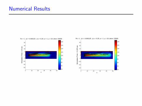
Numerical Results

0 10 20 30 40 50

−20

−15

−10

−5

0

5

10

15

20

28.5336928.5336939.96477

39.9647751.39586 51.3958662.82695 62.8269574.25804 74.2580485.68912 85.6891297.12021 97.12021108.5513 108.5513119.9824131.4135142.8446154.2756

x

Sim

ulat

ion

Tim

e =

2.5

sec

Pe = 1 ,∆ t = 0.000125 ,∆ x = 0.25 ,α = 1 ,u = 20 ,itime= 20000

20

40

60

80

100

120

140

160

180

0 10 20 30 40 50

−20

−15

−10

−5

0

5

10

15

20

28.50438 28.5043828.5043839.93742 39.93742

51.37046 51.3704662.8035 62.803574.23654 74.2365485.66958 85.6695897.10263 97.10263108.5357 108.5357119.9687131.4018142.8348154.2678

x

Sim

ulat

ion

Tim

e =

3.1

25 s

ec

Pe = 1 ,∆ t = 0.000125 ,∆ x = 0.25 ,α = 1 ,u = 20 ,itime= 25000

20

40

60

80

100

120

140

160

180

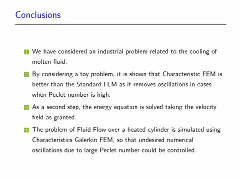
Conclusions

1 We have considered an industrial problem related to the cooling of

molten fluid.

2 By considering a toy problem, it is shown that Characteristic FEM is

better than the Standard FEM as it removes oscillations in cases

when Peclet number is high.

3 As a second step, the energy equation is solved taking the velocity

field as granted.

4 The problem of Fluid Flow over a heated cylinder is simulated using

Characteristics Galerkin FEM, so that undesired numerical

oscillations due to large Peclet number could be controlled.

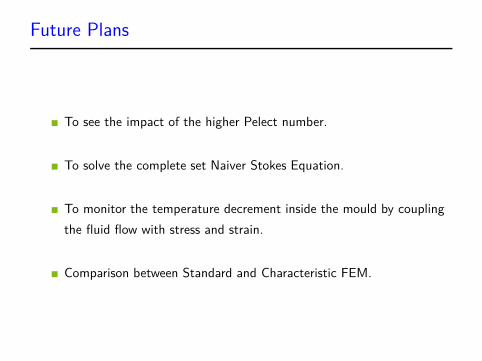
Future Plans

To see the impact of the higher Pelect number.

To solve the complete set Naiver Stokes Equation.

To monitor the temperature decrement inside the mould by coupling

the fluid flow with stress and strain.

Comparison between Standard and Characteristic FEM.

Bibliography

1 Roland. W. Lewis, P. Nithiarasu, and K. N. Seetharamu. Front

Matter. Wiley Online Library, 2004.

2 P. Nithiarasu, J. S. Mathur, N. P. Weatherill, and K. Morgan.

Three-dimensional incompressible flow calculations using the

characteristic based split (cbs) scheme. International Journal for

Numerical Methods in Fluids, 44(11),2004

3 E. O. Hate, R. L. Taylor, O. C. Zienkiewicz, and J. Rojek. A residual

correction method based on finite calculus. Engineering

Computations, 20(5/6), 2003.

4 K. Srinivas and C. A. J. Fletcher. Computational techniques for fluid

dynamics: a solutions manual. Springer, 1992.