A Novel Multilayer Neural Network Model for TOA-BasedLocalization in Wireless Sensor Networks

Sayed Yousef Monir Vaghefi, Reza Monir Vaghefi

Abstract—A novel multilayer neural network model, calledartificial synaptic network, was designed and implemented forsingle sensor localization with time-of-arrival (TOA) measure-ments. In the TOA localization problem, the location of a sourcesensor is estimated based on its distance from a number ofanchor sensors. The measured distance values are noisy andthe estimator should be able to handle different amounts ofnoise. Three neural network models: the proposed artificialsynaptic network, a multi-layer perceptron network, and ageneralized radial basis functions network were applied tothe TOA localization problem. The performance of the modelswas compared with one another. The efficiency of the modelswas calculated based on the memory cost. The study resultshows that the proposed artificial synaptic network has thelowest RMS error and highest efficiency. The robustness ofthe artificial synaptic network was compared with that ofthe least square (LS) method and the weighted least square(WLS) method. The Cramer-Rao lower bound (CRLB) of TOAlocalization was used as a benchmark. The model’s robustnessin high noise is better than the WLS method and remarkablyclose to the CRLB.

I. INTRODUCTION

W IRELESS sensor network (WSN) localization prob-lem is one of the interesting subjects studied in recent

years. In this problem, the locations of anchor sensors areknown and the location of each source sensor is estimatedbased on its distance from the anchor sensors. The approx-imate distance of a source sensor from an anchor sensoris obtained using different measurement methods such astime of arrival (TOA) [1], time difference of arrival [2],and received signal strength (RSS) [3]. Throughout thiswork we assume that the distances are obtained using TOAmeasurements, however, the problem can easily be extendedto the other methods.

The maximum likelihood (ML) estimator is the optimalestimator when the number of data records is sufficientlylarge [1], [4]. However, the cost function of the ML estimatoris non-linear and non-convex and finding the global minimumrequires convoluted computations. The solution of the MLestimator is computed using iterative optimization methods[1]. Since the cost function has many saddle points and localminima, a good initialization guess is inevitable to make surethat the algorithm converges to the global minimum. To dealwith this behavior of the ML estimator, different methodssuch as semidefinite programming (SDP) relaxation [5], [6]and multidimensional scaling (MDS) [7] are introduced.

Sayed Yousef Monir Vaghefi is with the School of Computer Scienceand Information Technology at Royal Melbourne Institute of Technology,Melbourne, Australia (email: s3268713@student.rmit.edu.au), Reza MonirVaghefi is with Department of Signals and Systems, Chalmers Universityof Technology, Gothenburg, Sweden (email: vaghefi@student.chalmers.se).

In SDP, the cost function is approximated and relaxed toa convex optimization problem and solved with efficientalgorithms that do not require any initialization. In MDS,the locations of the sources are estimated using data analysisof the coordinates and distances. It is stated that the MDSapproach is very sensitive to measurement noise and notapplicable to low connectivity networks [7].

Linear estimators [8], [9], [10] are also investigated in anumber of studies. The model of the TOA localization, whichis basically a non-linear problem, is linearized using someapproximation. The least squares (LS) method is studied in[9]. The method is simple to implement but cannot handlethe measurement noise. The TOA measurement noise isusually modeled as a zero-mean Gaussian random variablewith a variance depending mostly on the distances (i.e., thelarger measured distances have higher noise than the shorterones). To improve the performance of the LS method, theweighted least squares (WLS) algorithm [11] is introducedwhich can tolerate unequally sized noises. However, sincelinearization of the TOA localization model is done underthe assumption that the measurement noise is sufficientlysmall, the performance of LS and WLS declines considerablyas the measurement noise increases. Different extensionsto the LS method such as the constrained weighted leastsquares (CWLS) method [8] and corrected least squaresmethod [9] are also introduced. Although these algorithmshave better performance in high noise, their computation costand complexity is higher.

In this project, the TOA-based sensor localization is tack-led using artificial neural network models. Shareef et al.[12] have compared the performance of three types of neuralnetworks namely RBF, MLP, and recurrent neural networksin sensor localization. Their result shows that the RBFnetwork performs better than the other networks but it hashigher memory and computation costs. On the other hand,the MLP network has the lowest memory and computationcosts. Rahman et al. [13] have implemented a MLP networkfor the WSN localization problem. The network has reachedthe RMSe of 0.54 meter for a 20𝑚 × 20𝑚 problem. Thelocalization problem in a UWB sensor network is tackled in[14]. A neural network model is introduced. The performanceof the model has not been as good as the LS method. In[15], a neural network model is developed for identificationof undetected direct paths (UDP) in TOA localization.

The advantage of artificial neural network models is thatthey are adaptable to different conditions and situations.Indeed, our proposed model is designed to tolerate a specificcondition or situation. For instance, if the sensor network is

Proceedings of International Joint Conference on Neural Networks, San Jose, California, USA, July 31 – August 5, 2011

978-1-4244-9637-2/11/$26.00 ©2011 IEEE 3079

set up in an indoor environment where the signals from thesources are blocked and diminished by many objects and themeasurements are subject to high noise, the algorithm canbe trained to deal with the high-noise measurements. On theother hand, if the connectivity of the sensor network is highand it is required to have an accurate estimate, the algorithmcan be trained to handle the low-noise measurements.

The rest of paper is organized as follows. In the networkssection, the neural network models are described. In thedata section, the training and test data are presented. In theexperiments and results section, the models are comparedbased on their performance and efficiency and the robustnessof the artificial synaptic network (ASN) model is comparedwith that of the LS, and WLS methods. The study results aresummarized in the conclusion section.

II. NETWORKS

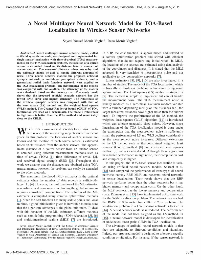
In this study, the TOA localization problem was consideredas a supervised learning problem, in which a neural networkis trained with a set of input-output data called the trainingdataset, and tested with another set of input-output data calledthe test dataset. Three neural network models: an artificialsynaptic network (ASN), a generalized radial basis func-tions (GRBF) network, and a multilayer preceptron (MLP)network were applied to the problem. The models wereimplemented in C sharp . The performance and efficiencyof the models were studied. The best model was identifiedand then tested for robustness. The designed ASN model iscomprised of a number of artificial synaptic networks - eachof them working on a data cluster. The architecture of eachnetwork is presented in Fig. 1. The output of each networkis computed using:

𝑓(𝑥) =

𝑛∑𝑖=1

𝑤𝑖 ∗ 𝑥𝑖 + 𝑤0. (1)

where n is the number of inputs, and is constructed in adeeper layer:

𝑤𝑖 =

𝑛∑𝑗=1

𝑤𝑖𝑗 ∗ 𝑥𝑗 + 𝑤𝑖0. (2)

where n is the number of inputs. In training, a center isassigned to each ASN by the k-means clustering algorithm.Each training data goes to the closet network. The error iscomputed at the output layer of the network. The error isthen backpropagated to the deepest layer. The weights at thedeepest layer are updated. The weights at the next layers arenot updated; they are instead constructed layer by layer fromthe weights of the deepest layer. The learning algorithm:

1. Initialize the centers, the output layer, the second layer,and the third layer weights, and the maximum acceptableerror

2. For each data pointa. Compute the Euclidean distance of the point from all

the centersb. Assign the closet center to the point

Fig. 1. Artificial Synaptic Network (ASN) architecture

3080

3. For each centerChange the center to the centroid of the data points

assigned to that center4. If not yet converged go to step 25. For each data point: xa. 𝑏𝑎𝑐𝑘𝑝𝑟𝑜𝑝𝑎𝑔𝑎𝑡𝑒(𝑥)b. Compute the networks output:𝑛𝑒𝑡𝑤𝑜𝑟𝑘𝑜𝑢𝑡(𝑥) = 𝑐𝑜𝑚𝑝𝑢𝑡𝑒𝑜𝑢𝑡𝑝𝑢𝑡(𝑥)

Fig. 2. Multilayer Preceptron Network Architecture

Fig. 3. GRBF Network Architecture

6. Compute the Root Mean Square Error:

𝑟𝑚𝑠𝑒 =

√∑𝑛𝑖=1 (𝑜𝑢𝑡𝑝𝑢𝑡𝑖 − 𝑛𝑒𝑡𝑤𝑜𝑟𝑘𝑜𝑢𝑡𝑖)

2

𝑛(3)

where n is the number of training data.7. If (𝑟𝑚𝑠𝑒 > 𝑚𝑎𝑥𝑒𝑟𝑟𝑜𝑟) go to step 5The computeoutput(x: the data point) method:1. Compute the Euclidean distance of x from all the centers2. Send x to the network with the closet center3. Compute the output of the chosen network:

𝑤𝑖 =

𝑛∑𝑗=1

𝑤𝑖𝑗 ∗ 𝑥𝑗 + 𝑤𝑖0. (4)

−20 −15 −10 −5 0 5 10 15 20

−20

−15

−10

−5

0

5

10

15

20

x coordinate [m]

y co

ordi

nate

[m]

Fig. 4. Training dataset

−20 −15 −10 −5 0 5 10 15 20

−20

−15

−10

−5

0

5

10

15

20

x coordinate [m]

y co

ordi

nate

[m]

Fig. 5. Test dataset

𝑛𝑒𝑡𝑤𝑜𝑟𝑘𝑜𝑢𝑡(𝑥) =

𝑛∑𝑖=1

𝑤𝑖 ∗ 𝑥𝑖 + 𝑤0. (5)

where n is the number of inputs.The backpropagation(x:the data point) method:1. Compute the output for the data point:𝑐𝑜𝑚𝑝𝑢𝑡𝑒𝑜𝑢𝑡𝑝𝑢𝑡(𝑥)2. Backpropagate the error layer by layera. Output layer:𝑑𝑒𝑙𝑡𝑎1 = 𝑜𝑢𝑡𝑝𝑢𝑡(𝑥)− 𝑛𝑒𝑡𝑤𝑜𝑟𝑘𝑜𝑢𝑡(𝑥)b. Second layer:𝑑𝑒𝑙𝑡𝑎2𝑖 = 𝑑𝑒𝑙𝑡𝑎1 ∗ 𝑥𝑖

c. Third layer:𝑑𝑒𝑙𝑡𝑎3𝑖𝑗 = 𝑑𝑒𝑙𝑡𝑎2𝑖 ∗ 𝑥𝑗

3. Update the weights of the deepest layer𝑙𝑎𝑦𝑒𝑟3𝑤𝑒𝑖𝑔ℎ𝑡𝑠 = 𝑙𝑎𝑦𝑒𝑟3𝑤𝑒𝑖𝑔ℎ𝑡𝑠+ 𝑒𝑡𝑎 ∗ 𝑑𝑒𝑙𝑡𝑎3 ∗ 𝑥

3081

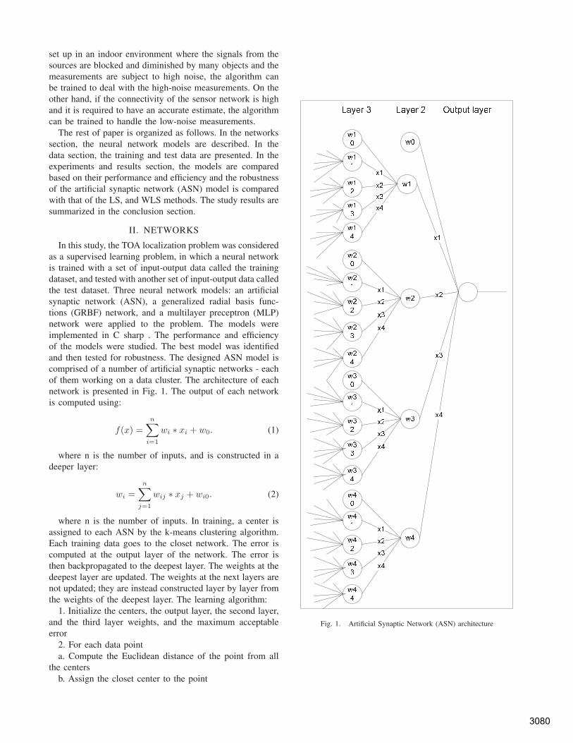
The multilayer preceptron (MLP) network implementedfor the problem has two hidden layers. The architecture ofthe network is presented in Fig. 2. The activation function ofthe hidden neurons is a logistic function. The network wastrained using the backpropagation algorithm [16].

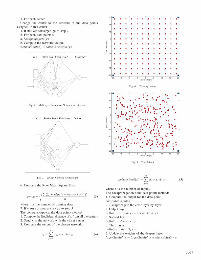
The GRBF network [17] consists of a number of radialbasis function neurons, each of them working on a center.In the training, the fixed centers of the network are specifiedusing the k-means clustering algorithm. The network is thentrained using the gradient descent algorithm. Fig. 3 showsthe architecture of the network.

III. DATA

The performance of a neural network model dependson the density of the training data and complexity of theproblem. If the training data is not dense, the network doesnot have enough information to build the model. Consideringthe modeling process as a hyperplane reconstruction process,the more complex the hyperplane is the more data is requiredfor reconstruction.

The datasets were generated in MATLAB. The trainingdataset was a set of 144 data points evenly distributed overthe input space. Fig. 4 presents the training dataset. Thered points, diamonds, are the source sensors and the bluepoints, squares, are the anchors. The test dataset was 300data points randomly distributed over the input space. Thedistances of each data point from the anchors were calculatedby MATLAB. A random amount of noise was added to thedistances. The test dataset is shown in the Fig. 5.

IV. EXPERIMENTS AND RESULTS

A model with two outputs is required to estimate thelocation, x and y, of a sensor. However, since one-outputmodels have less complexity and less training time, twoseparate models of one output were employed to estimatex and y of a sensor. In the first experiment the models weretrained with the training dataset of Fig. 4. The performanceof the models was compared based on the Root Mean Squareerror (RMSe). The efficiency of the models was comparedbased on the memory cost. Table 1 shows the memory costand RMSe of the models.

The memory cost was calculated based on the number ofmemory blocks required to store the centers and synapticweights. In the GRBF network, there are 15 centers thatrequire 60 memory blocks, and there are 15 synaptic weightsthat require 15 blocks of memory. The MLP network has7 neurons in each hidden layer which means 28 synapticweights between the input layer and the first hidden layer,49 synaptic weights between the first and the second hiddenlayer, and 7 synaptic weights between the second hiddenlayer and the output layer. The number of synaptic weights inthe ASN model is equal to the number of centers multipliedby the number of neurons in the deepest layer. The modelhas 3 centers and there are 20 neurons in the deepest layer.

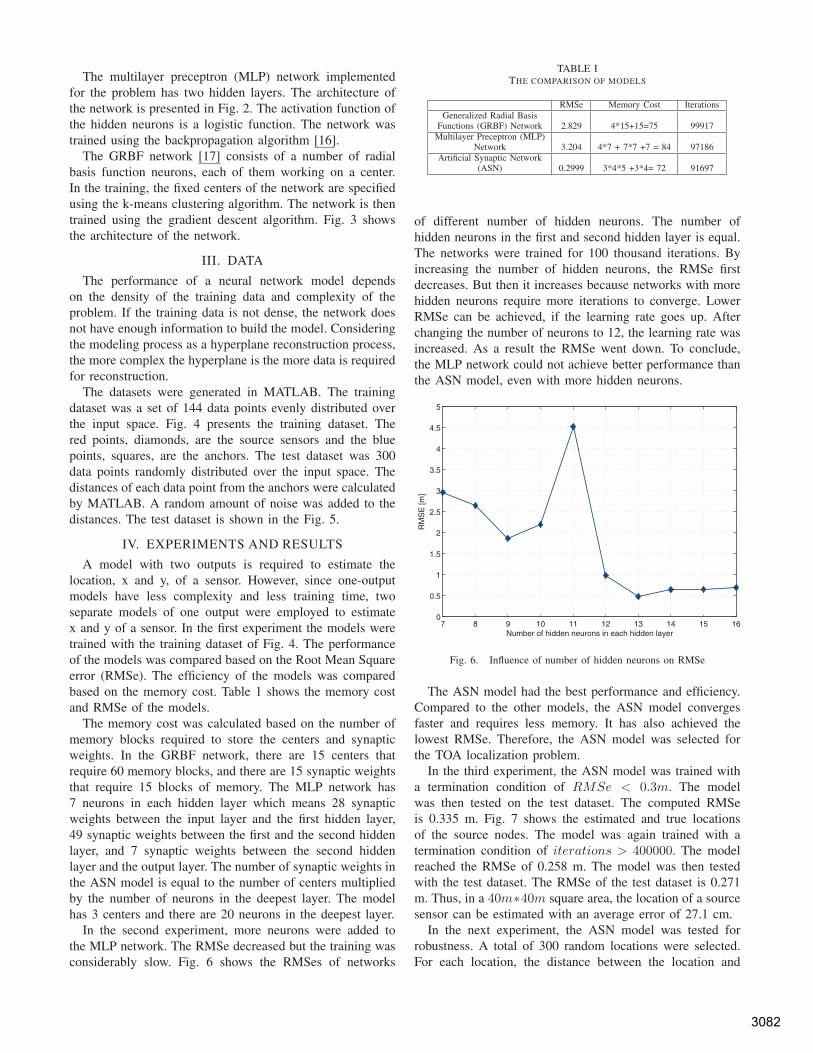
In the second experiment, more neurons were added tothe MLP network. The RMSe decreased but the training wasconsiderably slow. Fig. 6 shows the RMSes of networks

TABLE ITHE COMPARISON OF MODELS

RMSe Memory Cost IterationsGeneralized Radial Basis

Functions (GRBF) Network 2.829 4*15+15=75 99917Multilayer Preceptron (MLP)

Network 3.204 4*7 + 7*7 +7 = 84 97186Artificial Synaptic Network

(ASN) 0.2999 3*4*5 +3*4= 72 91697

of different number of hidden neurons. The number ofhidden neurons in the first and second hidden layer is equal.The networks were trained for 100 thousand iterations. Byincreasing the number of hidden neurons, the RMSe firstdecreases. But then it increases because networks with morehidden neurons require more iterations to converge. LowerRMSe can be achieved, if the learning rate goes up. Afterchanging the number of neurons to 12, the learning rate wasincreased. As a result the RMSe went down. To conclude,the MLP network could not achieve better performance thanthe ASN model, even with more hidden neurons.

7 8 9 10 11 12 13 14 15 160

0.5

1

1.5

2

2.5

3

3.5

4

4.5

5

Number of hidden neurons in each hidden layer

RM

SE

[m]

Fig. 6. Influence of number of hidden neurons on RMSe

The ASN model had the best performance and efficiency.Compared to the other models, the ASN model convergesfaster and requires less memory. It has also achieved thelowest RMSe. Therefore, the ASN model was selected forthe TOA localization problem.

In the third experiment, the ASN model was trained witha termination condition of 𝑅𝑀𝑆𝑒 < 0.3𝑚. The modelwas then tested on the test dataset. The computed RMSeis 0.335 m. Fig. 7 shows the estimated and true locationsof the source nodes. The model was again trained with atermination condition of 𝑖𝑡𝑒𝑟𝑎𝑡𝑖𝑜𝑛𝑠 > 400000. The modelreached the RMSe of 0.258 m. The model was then testedwith the test dataset. The RMSe of the test dataset is 0.271m. Thus, in a 40𝑚∗40𝑚 square area, the location of a sourcesensor can be estimated with an average error of 27.1 cm.

In the next experiment, the ASN model was tested forrobustness. A total of 300 random locations were selected.For each location, the distance between the location and

3082

each anchor was computed. A zero-mean Gaussian noisewas added to the distances. A set of 10 different four-distance inputs were computed for each location. A total of3000 inputs were sent to the ASN model and the RMSewas computed. The experiment was repeated for different

−20 −15 −10 −5 0 5 10 15 20

−20

−15

−10

−5

0

5

10

15

20

x coordinate [m]

y co

ordi

nate

[m]

Fig. 7. Diamonds depict estimated locations and squares depict truelocations.

Gaussian noises. Two other methods applied to the WSNlocalization problem, the LS method and the WLS method,were tested using the same procedure. Fig. 8 shows thecomputed RMSe in the presence of different amounts ofnoise. As shown in the figure, although the ASN modelhas achieved lower RMSes compared to the LS method, themodel has not been as robust as the WLS method.

To improve the robustness of the model, two centers wereadded to the model. The memory cost increased to 100.The model was trained using the same training dataset. Thetraining stopped with the RMSe of 0.3 m. The model wastested with the same set of test inputs. Fig. 9 presents therobustness of the model. As shown in the figure, the modelis almost as robust as the WLS method. However, WLSoutperforms the model when the standard deviation of noiseis lower than 0.5.

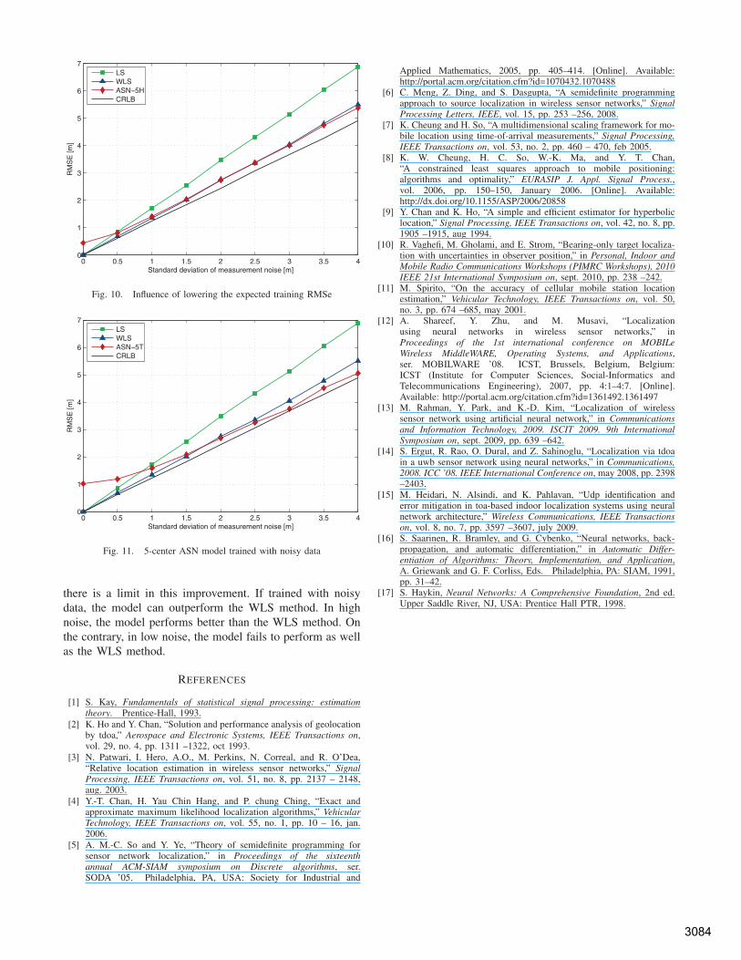
If the model is less trained, it would be more robust. Inother words, if the RMSe of the training data is higher, themodel’s tolerance of noise is higher. To test this theory,the model was trained with the termination condition of𝑅𝑀𝑆𝑒 < 0.5𝑚. The model was then tested on the testdataset. Fig. 10 compares the model’s robustness with thatof the other methods. As demonstrated by this figure, whenthe noise standard deviation is higher than or equal to 2,the model has lower RMSes compared to the WLS method.Conversely, when the noise standard deviation is lower than2, the model has higher RMSes in compare with the WLSmethod.

Another way to improve the robustness is to train themodel with noisy data. A zero-mean Gaussian noise with thestandard deviation of 2 was added to the training data. The

0 0.5 1 1.5 2 2.50

0.5

1

1.5

2

2.5

3

3.5

4

4.5

Standard deviation of measurement noise [m]

RM

SE

[m]

LSWLSASN−3CRLB

Fig. 8. ASN model with 3 centers

0 0.5 1 1.5 2 2.5 3 3.5 40

1

2

3

4

5

6

7

Standard deviation of measurement noise [m]

RM

SE

[m]

LSWLSASN−5CRLB

Fig. 9. ASN model with 5 centers

model was trained with the new training dataset. The modelwas then tested with the same test inputs. Fig. 11 shows theresults. When the noise is high, the model outperforms theWLS method. In contrast, when the noise is low, the modelfails to compete with the WLS method. Overall, the model’srobustness is better than the LS method and almost as goodas the WLS method. If trained with noisy data, the modelcan outperform the WLS method.

V. CONCLUSION

In TOA localization, our artificial synaptic network (ASN)model has better performance and efficiency compared toGRBF and MLP models. The model converges faster andits memory cost is lower. Tested on the training dataset, themodel reached the RMSe of 0.258 m. Tried on the test datasetthe model achieved the RMSe of 0.271 m. Therefore, in a40 m * 40 m square area, the location of a source sensor canbe estimated with an average error of 27.1 cm.

The robustness of the ASN model is almost as well as theweighted least squares (WLS) method. Adding more centersto the model improves the robustness of the model. However,

3083

0 0.5 1 1.5 2 2.5 3 3.5 40

1

2

3

4

5

6

7

Standard deviation of measurement noise [m]

RM

SE

[m]

LSWLSASN−5HCRLB

Fig. 10. Influence of lowering the expected training RMSe

0 0.5 1 1.5 2 2.5 3 3.5 40

1

2

3

4

5

6

7

Standard deviation of measurement noise [m]

RM

SE

[m]

LSWLSASN−5TCRLB

Fig. 11. 5-center ASN model trained with noisy data

there is a limit in this improvement. If trained with noisydata, the model can outperform the WLS method. In highnoise, the model performs better than the WLS method. Onthe contrary, in low noise, the model fails to perform as wellas the WLS method.

REFERENCES

[1] S. Kay, Fundamentals of statistical signal processing: estimationtheory. Prentice-Hall, 1993.

[2] K. Ho and Y. Chan, “Solution and performance analysis of geolocationby tdoa,” Aerospace and Electronic Systems, IEEE Transactions on,vol. 29, no. 4, pp. 1311 –1322, oct 1993.

[3] N. Patwari, I. Hero, A.O., M. Perkins, N. Correal, and R. O’Dea,“Relative location estimation in wireless sensor networks,” SignalProcessing, IEEE Transactions on, vol. 51, no. 8, pp. 2137 – 2148,aug. 2003.

[4] Y.-T. Chan, H. Yau Chin Hang, and P. chung Ching, “Exact andapproximate maximum likelihood localization algorithms,” VehicularTechnology, IEEE Transactions on, vol. 55, no. 1, pp. 10 – 16, jan.2006.

[5] A. M.-C. So and Y. Ye, “Theory of semidefinite programming forsensor network localization,” in Proceedings of the sixteenthannual ACM-SIAM symposium on Discrete algorithms, ser.SODA ’05. Philadelphia, PA, USA: Society for Industrial and

Applied Mathematics, 2005, pp. 405–414. [Online]. Available:http://portal.acm.org/citation.cfm?id=1070432.1070488

[6] C. Meng, Z. Ding, and S. Dasgupta, “A semidefinite programmingapproach to source localization in wireless sensor networks,” SignalProcessing Letters, IEEE, vol. 15, pp. 253 –256, 2008.

[7] K. Cheung and H. So, “A multidimensional scaling framework for mo-bile location using time-of-arrival measurements,” Signal Processing,IEEE Transactions on, vol. 53, no. 2, pp. 460 – 470, feb 2005.

[8] K. W. Cheung, H. C. So, W.-K. Ma, and Y. T. Chan,“A constrained least squares approach to mobile positioning:algorithms and optimality,” EURASIP J. Appl. Signal Process.,vol. 2006, pp. 150–150, January 2006. [Online]. Available:http://dx.doi.org/10.1155/ASP/2006/20858

[9] Y. Chan and K. Ho, “A simple and efficient estimator for hyperboliclocation,” Signal Processing, IEEE Transactions on, vol. 42, no. 8, pp.1905 –1915, aug 1994.

[10] R. Vaghefi, M. Gholami, and E. Strom, “Bearing-only target localiza-tion with uncertainties in observer position,” in Personal, Indoor andMobile Radio Communications Workshops (PIMRC Workshops), 2010IEEE 21st International Symposium on, sept. 2010, pp. 238 –242.

[11] M. Spirito, “On the accuracy of cellular mobile station locationestimation,” Vehicular Technology, IEEE Transactions on, vol. 50,no. 3, pp. 674 –685, may 2001.

[12] A. Shareef, Y. Zhu, and M. Musavi, “Localizationusing neural networks in wireless sensor networks,” inProceedings of the 1st international conference on MOBILeWireless MiddleWARE, Operating Systems, and Applications,ser. MOBILWARE ’08. ICST, Brussels, Belgium, Belgium:ICST (Institute for Computer Sciences, Social-Informatics andTelecommunications Engineering), 2007, pp. 4:1–4:7. [Online].Available: http://portal.acm.org/citation.cfm?id=1361492.1361497

[13] M. Rahman, Y. Park, and K.-D. Kim, “Localization of wirelesssensor network using artificial neural network,” in Communicationsand Information Technology, 2009. ISCIT 2009. 9th InternationalSymposium on, sept. 2009, pp. 639 –642.

[14] S. Ergut, R. Rao, O. Dural, and Z. Sahinoglu, “Localization via tdoain a uwb sensor network using neural networks,” in Communications,2008. ICC ’08. IEEE International Conference on, may 2008, pp. 2398–2403.

[15] M. Heidari, N. Alsindi, and K. Pahlavan, “Udp identification anderror mitigation in toa-based indoor localization systems using neuralnetwork architecture,” Wireless Communications, IEEE Transactionson, vol. 8, no. 7, pp. 3597 –3607, july 2009.

[16] S. Saarinen, R. Bramley, and G. Cybenko, “Neural networks, back-propagation, and automatic differentiation,” in Automatic Differ-entiation of Algorithms: Theory, Implementation, and Application,A. Griewank and G. F. Corliss, Eds. Philadelphia, PA: SIAM, 1991,pp. 31–42.

[17] S. Haykin, Neural Networks: A Comprehensive Foundation, 2nd ed.Upper Saddle River, NJ, USA: Prentice Hall PTR, 1998.

3084