Citation: Mehbodniya, A.;

Douraki, B.k.; Webber, J.L.;

Alkhazaleh, H.A.; Elbasi, E.;

Dameshghi, M.; Abu Zitar, R.;

Abualigah, L. Multilayer Reversible

Data Hiding Based on the Difference

Expansion Method Using Multilevel

Thresholding of Host Images Based

on the Slime Mould Algorithm.

Processes 2022, 10, 858. https://

doi.org/10.3390/pr10050858

Academic Editor: Mengchu Zhou

Received: 16 March 2022

Accepted: 24 April 2022

Published: 26 April 2022

Publisher’s Note: MDPI stays neutral

with regard to jurisdictional claims in

published maps and institutional affil-

iations.

Copyright: © 2022 by the authors.

Licensee MDPI, Basel, Switzerland.

This article is an open access article

distributed under the terms and

conditions of the Creative Commons

Attribution (CC BY) license (https://

creativecommons.org/licenses/by/

4.0/).

processes

Article

Multilayer Reversible Data Hiding Based on the DifferenceExpansion Method Using Multilevel Thresholding of HostImages Based on the Slime Mould AlgorithmAbolfazl Mehbodniya 1 , Behnaz karimi Douraki 2, Julian L. Webber 1, Hamzah Ali Alkhazaleh 3,* ,Ersin Elbasi 4 , Mohammad Dameshghi 5, Raed Abu Zitar 6 and Laith Abualigah 7

1 Department of Electronics and Communication Engineering, Kuwait College of Science andTechnology (KCST), Kuwait City 7207, Kuwait; a.niya@kcst.edu.kw (A.M.); jwebber@ieee.org (J.L.W.)

2 Department of Mathematics, University of Isfahan, Isfahan 81431-33871, Iran; bkarimidouraki@gmail.com3 IT Department, College of Engineering and IT, University of Dubai, Academic City, United Arab Emirates4 College of Engineering and Technology, American University of the Middle East, Kust Kuwait 15453, Kuwait;

ersin.elbasi@aum.edu.kw5 Department of Computer Engineering, Faculty of Electrical and Computer Engineering, University of Tabriz,

Tabriz 5166-15731, Iran; dameshghi@aol.com6 Sorbonne Center of Artificial Intelligence, Sorbonne University-Abu Dhabi, Abu Dhabi, United Arab Emirates;

raed.zitar@sorbonne.ae7 Faculty of Computer Sciences and Informatics, Amman Arab University, Amman 11953, Jordan;

aligah.2020@gmail.com* Correspondence: halkhazaleh@ud.ac.ae

Abstract: Researchers have scrutinized data hiding schemes in recent years. Data hiding in standardimages works well, but does not provide satisfactory results in distortion-sensitive medical, military,or forensic images. This is because placing data in an image can cause permanent distortion afterdata mining. Therefore, a reversible data hiding (RDH) technique is required. One of the well-knowndesigns of RDH is the difference expansion (DE) method. In the DE-based RDH method, findingspaces that create less distortion in the marked image is a significant challenge, and has a highinsertion capacity. Therefore, the smaller the difference between the selected pixels and the morecorrelation between two consecutive pixels, the less distortion can be achieved in the image afterembedding the secret data. This paper proposes a multilayer RDH method using the multilevelthresholding technique to reduce the difference value in pixels and increase the visual quality andthe embedding capacity. Optimization algorithms are one of the most popular methods for solvingNP-hard problems. The slime mould algorithm (SMA) gives good results in finding the best solutionsto optimization problems. In the proposed method, the SMA is applied to the host image for optimalmultilevel thresholding of the image pixels. Moreover, the image pixels in different and more similarareas of the image are located next to one another in a group and classified using the specifiedthresholds. As a result, the embedding capacity in each class can increase by reducing the value ofthe difference between two consecutive pixels, and the distortion of the marked image can decreaseafter inserting the personal data using the DE method. Experimental results show that the proposedmethod is better than comparable methods regarding the degree of distortion, quality of the markedimage, and insertion capacity.

Keywords: reversible data hiding (RDH); slime mould algorithm (SMA); difference expansion (DE)

1. Introduction

Data hiding (DH) is a way of secretly sending information or data to others. In thisway, data, including text, images, etc., can be inserted into a medium such as an image,video, audio, etc., using a DH algorithm to make them invisible to others. DH is performedin two domains of space and frequency. The related data are inserted directly into the

Processes 2022, 10, 858. https://doi.org/10.3390/pr10050858 https://www.mdpi.com/journal/processes

Processes 2022, 10, 858 2 of 24

host image pixels in the space domain, which is often reversible. Reversibility meansthat the inserted data and the original host image are entirely recovered in the extractionphase. In the frequency domain, first, a frequency transform such as discrete wavelettransform (DWT), discrete cosine transform (DCT), etc., is applied to the host image. Then,using a special algorithm, the data are inserted into frequency coefficients that are oftenirreversible. The data are then extracted, while the original host image is not fully andaccurately recovered.

Reversible data hiding (RDH) techniques in the space field are divided into severalcategories: difference expansion (DE), histogram shifting (HS), prediction-error expansion(PEE), pixel value grouping (PVG), and pixel value ordering (PVO). Over the years, variousRDH methods have been proposed by researchers in these fields, all of which aim to reducedistortion and increase the quality of the marked image or increase the capacity to insertthe data, and these issues continue. As the main challenge, this has occupied the minds ofresearchers. The following is a brief description of the papers available in each field:

An RDH method was proposed in [1] to increase the capacity based on the DE method.In this method, the host image is divided into 1 × 2 blocks, and spaces of −1, 0, and +1 areselected to insert the data. A lossless RDH method based on the DE histogram (DEH) wasproposed to increase the capacity in [2], where the difference histogram (DH) peak pointwas selected to insert the data. In [3], a multilayer RDH method based on the DEH wasproposed to increase the capacity and reduce the distortion. However, this method wasnot able to improve the capacity sufficiently. In [4], the RDH method was presented forgray images using the DEH and the module function. The position matrix and the markedimage were sent separately to the receiver with low capacity.

In [5], to improve the capacity performance and increase security, a guided filterpredictor and an adaptive PEE design were used to insert the data in color images usingintrachannel correlation. A two-layer DH method based on the expansion and displacementof a PE pair in a two-dimensional histogram was proposed to increase the capacity byextracting the correlations between the consecutive PEs in [6], where their work was bothlow-capacity and low-quality. In [7], the authors presented an RDH method based on themultiple histogram correction and PEE to increase the capacity of the gray images, using arhombus predictor to predict the host image pixels. In PE histogram (PEH) methods [8], toextract the redundancy between adjacent pixels, the correction path detection strategy isused to obtain a two-dimensional PEH that has a high distortion. In an RDH method [9],based on a two-layer insertion and PEH, the pixel pairs are selected based on pixel densityand the spatial distance between two pixels. The distortion is much less than in the previousmethods. In [10], an RDH method based on multiple histogram shifting was proposedthat used a genetic algorithm (GA) to control the substantial image distortion. In [11], anRDH technique was proposed based on pairwise prediction-error expansion (PPEE) ortwo-dimensional PEH (2D-PEH) to increase capacity. In [12], an RDH technique based onthe host image texture analysis was proposed by blocking the image and inserting the datainto image texture blocks [13–20].

In another RDH method [21], the PVG method was used by multilayer insertion toincrease the capacity. The PVG was applied on each block. The zero point of the histogramof the difference was selected to insert the data bits. The pixel-based PVG (PPVG) techniquein [22] was proposed to increase the capacity applied to each block after image blocking.Each time a pixel is located in the smooth areas of each block for inserting the data, the PEvalue is the difference between the reference pixel and the particular pixel. This method hasa low capacity and moderate distortion. In [23], a technique was presented to increase thereliability of the image for inserting the data. Using PEE based on PVO, the authors insertedthe data in the pins of −1 and +1 from the PEH. The problem was that the quality of theimage was still low, while the capacity was not high. The authors of [24] presented a robustreversible data hiding (RRDH) scheme based on two-layer embedding with a reducedcapacity-distortion tradeoff, where it first decomposes the image into two planes—namely,

Processes 2022, 10, 858 3 of 24

the higher significant bit (HSB) and least important bit (LSB) planes—and then employsprediction-error expansion (PEE) to embed the secret data into the HSB plane.

In [25], the authors proposed an AMBTC-based RDH method in which the hammingdistance and PVD methods were used to insert information. In [26], a PVD-based RDHmethod was used. In [27], the RDH method was based on PVD and LSB reversible insertinformation. The authors of [28] proposed an RDH in encrypted images (RDHEI) methodwith hierarchical embedding based on PE. PEs are divided into three categories: small-magnitude, medium-magnitude, and large-magnitude. In their approach, pixels withsmall-magnitude/large-magnitude PEs were used to insert data. Their method had a highcapacity, but the image quality was still low.

The authors of [29] proposed an RDH method for color images using HS-based double-layer embedding. The authors used the image interpolation method to generate PE matricesfor HS in the first-layer embedding, and local pixel similarity to calculate the differencematrices for HS in the second-layer embedding. In their process, the embedding capacitywas low. In [30], the authors proposed a dual-image RDH method based on PE shift. More-over, in their work, a bidirectional-shift strategy was used to extend the shiftable positionsin the central zone of the allowable coordinates. In their work, the embedding capacitywas low. Today, optimization algorithms such as the grasshopper optimization algorithm(GOA), whale optimization algorithm (WOA), moth–flame optimization (MFO) [31], Harrishawk optimization (HHO) [32], and artificial bee colony (ABC) [33] are used in manypapers [34–38].

This paper proposes a DE-based multilayer image RDH method using the multilevelthresholding technique. Optimization algorithms are one of the most popular methodsfor solving NP-hard problems. Due to this, the slime mould algorithm (SMA) gives goodresults in finding the best solutions to solve optimization problems. First, the SMA isapplied to the host image to find the two thresholds, and image pixels are based on thethresholds located in three different classes. Using the multilevel thresholding creates moresimilarities between the pixels of each class. Therefore, due to the reduction in the differencebetween each class’ pixels, the quality of the marked image does not decrease with theinsertion of data via DE. At the same time, less distortion is created in the picture, and theinsertion capacity increases. Table 1 shows the critical acronyms and their meanings.

Table 1. Key acronyms and their meanings.

Key Acronyms Their Meanings

DH Data hiding

DWT Discrete wavelet transform

DCT Discrete cosine transform

RDH Reversible data hiding

DE Difference expansion

HS Histogram shifting

PEE Prediction-error expansion

PVG Pixel value grouping

PVO Pixel value ordering

DH Difference histogram

PEH PE histogram

GA Genetic algorithm

PPEE Pairwise prediction-error expansion

2D-PEH Two-dimensional PEH

Processes 2022, 10, 858 4 of 24

Table 1. Cont.

Key Acronyms Their Meanings

RRDH Robust reversible data hiding

HSB Higher significant bit

LSB Least important bit

PEE Prediction-error expansion

RDHEI RDH in encrypted images

MSE Mean squared error

PSNR Peak signal-to-noise ratio

bpp Bits per pixel

SSIM Structural similarity index measure

The method of Arham et al. [3] is the basis of the proposed method. Arham et al. [3]proposed a multilayer RDH method to reduce the distortion in the image. First, the hostimage is divided into 2 × 2 blocks in their work. Then, to calculate the value of differencesfor both consecutive pixels, the pixel vector is created for each block in each layer, as shownin Figure 1. A threshold (2 ≤ Th ≤ 30) is considered, and only the blocks in which thevalue of differences for both consecutive pixels is positive and less than the threshold value(2 ≤ Th ≤ 30) are selected to insert the data.

Processes 2022, 10, x FOR PEER REVIEW 4 of 24

GA Genetic algorithm

PPEE Pairwise prediction-error expansion

2D-PEH Two-dimensional PEH

RRDH Robust reversible data hiding

HSB Higher significant bit

LSB Least important bit

PEE Prediction-error expansion

RDHEI RDH in encrypted images

MSE Mean squared error

PSNR Peak signal-to-noise ratio

bpp Bits per pixel

SSIM Structural similarity index measure

The method of Arham et al. [3] is the basis of the proposed method. Arham et al. [3]

proposed a multilayer RDH method to reduce the distortion in the image. First, the host

image is divided into 2 × 2 blocks in their work. Then, to calculate the value of differences

for both consecutive pixels, the pixel vector is created for each block in each layer, as

shown in Figure 1. A threshold (2 ≤ Th ≤ 30) is considered, and only the blocks in which

the value of differences for both consecutive pixels is positive and less than the threshold

value (2 ≤ Th ≤ 30) are selected to insert the data.

Figure 1. Production of vectors for four layers [3]: (a) Layer-1; (b) Layer-2; (c) Layer-3; (d) Layer-4.

For each the vectors ws where s = {0, 1, 2, 3} in the s-th insertion layer, in order to

ensure reversibility and extract the data in the extraction phase, the s-th pixel from each

block is not inserted, there is a reference pixel in each insertion layer, and three bits of data

are inserted in a block of size 2 × 2. In the first insertion layer, in Figure 1, the pixel vector

ws is created to calculate the values of v1, v2, v3,. The value of differences is calculated

using Equation (1) for both consecutive pixels:

v1 = u1 − u0, v2 = u2 − u1, v3 = u3 − u2 (1)

Furthermore, to reduce the distortion and control of overflow/underflow, Equation

(2) is used to reduce the value of vk (k = 1, 2, 3):

vk′ = {

vk − 2|vk|−1 if 2 × 2n−1 ≤ |vk| ≤ 3 × 2

n−1 − 1

vk − 2|vk| if 3 × 2n−1 ≤ |vk| ≤ 4 × 2n−1 − 1

(2)

where n is calculated using Equation (3):

n = ⌊log2(|vk|)⌋ (3)

Then, the value of vk″ is expanded to Equation (4) by collecting the kth bits of the

three-bit sequence of confidential data b = (b1, b2, b3), as follows:

vk″ = 2 × vk

′ + bk (4)

Figure 1. Production of vectors for four layers [3]: (a) Layer-1; (b) Layer-2; (c) Layer-3; (d) Layer-4.

For each the vectors ws where s = {0, 1, 2, 3} in the s-th insertion layer, in order toensure reversibility and extract the data in the extraction phase, the s-th pixel from eachblock is not inserted, there is a reference pixel in each insertion layer, and three bits of dataare inserted in a block of size 2 × 2. In the first insertion layer, in Figure 1, the pixel vectorws is created to calculate the values of v1, v2, v3,. The value of differences is calculatedusing Equation (1) for both consecutive pixels:

v1= u1 − u0, v2 = u2 − u1, v3 = u3 − u2 (1)

Furthermore, to reduce the distortion and control of overflow/underflow, Equation (2)is used to reduce the value of vk (k = 1, 2, 3):

v′k =

{vk − 2|vk|−1 if 2× 2n−1 ≤ |vk| ≤ 3× 2n−1 − 1vk − 2|vk| if 3× 2n−1 ≤ |vk| ≤ 4× 2n−1 − 1

(2)

where n is calculated using Equation (3):

n = blog2 (|vk|)c (3)

Processes 2022, 10, 858 5 of 24

Then, the value of v′′k is expanded to Equation (4) by collecting the kth bits of thethree-bit sequence of confidential data b = (b1, b2, b3), as follows:

v′′k= 2 × v′k+bk (4)

A location map (LM) is used to separate the range |vk|, as shown in Equation (5),to recover the original differences and the original pixels of the host image in the extrac-tion phase:

LM =

{0, if 2× 2n−1 ≤ |vk| ≤ 3× 2n−1 − 11, if 3× 2n−1 ≤ |vk| ≤ 4× 2n−1 − 1

(5)

Each insertion layer creates a location map (M) to determine the location of blockscontaining data. If the block is inserted with the data bits, the value of M is equal to1. Otherwise, the value of M is 0. Finally, Equation (6) is used to insert the data in thevector u0:

v0 = u0+ u1+ u2+ u32

u0 = u0, u1 = v′′1 + u0, u2 = v′′2 + u2, u3 = v′′3 + u3(6)

In the extraction phase, the secret data and the vk are recovered using location mapsLM and M and Equation (7):

vk =

{v′k +

(∣∣v′k∣∣)+ 1, if LM = 0v′k +

(∣∣v′k∣∣), if LM = 1(7)

The remainder of this paper is organized as follows: Section 2 introduces the proposedplan that uses the Otsu thresholding method and SMA. In Section 3, the proposed methodsare evaluated and compared with other works, and Section 4 contains the conclusions.

2. Proposed Method

The proposed method consists of three phases: In the first phase, the multilevelthresholding technique using a combination of the SMA and the Otsu evaluation functionis applied to the host image to classify the host image pixels based on the relevant thresholds.The second phase inserts the data in the pixels of each class using DE, and in the thirdphase the extracted inserted data and the original image are recovered. In the followingsection, each of these three phases is described in turn:

2.1. Multilevel Thresholding Using the Slime Mould Algorithm

In the DE-based DH methods, the extraction of the best and most extra space forinserting the data and achieving a high capacity will also create less distortion in the hostimage—a significant issue. In other words, the smaller the difference between the twoconsecutive pixels and the more similarity between the pixels, the less distortion created inthe image after inserting the data using the DE.

In this paper, we use the multilevel thresholding technique using the combination ofthe SMA and the Otsu evaluation function [34] to determine the two optimal thresholds (T1and T2) for classifying the image pixels. Thus, increases in the similarity and correlation be-tween the pixels of each class are used to reduce the value of differences for two consecutivepixels in each class, and to increase capacity and reduce distortion in the marked image.

The Otsu method is an automatic thresholding method obtained according to theimage histogram, and defines the boundaries of objects in the image with high accuracy [34].In gray images, the pixel intensity is between 0 and 255. Therefore, the Otsu method selectsa threshold from 0 to 255, with the highest interclass variance in gray images, or minimizesintraclass variance [34]. All image pixels are grouped using multilevel thresholding basedon correlation and similarity [35].

SMA is a new population-based metaheuristic algorithm [36] inspired by the intelligentbehavior of a type of mould called slime mould. Slime mould also behaves intelligently,and can navigate very quickly and without error. In this paper, the input and output of the

Processes 2022, 10, 858 6 of 24

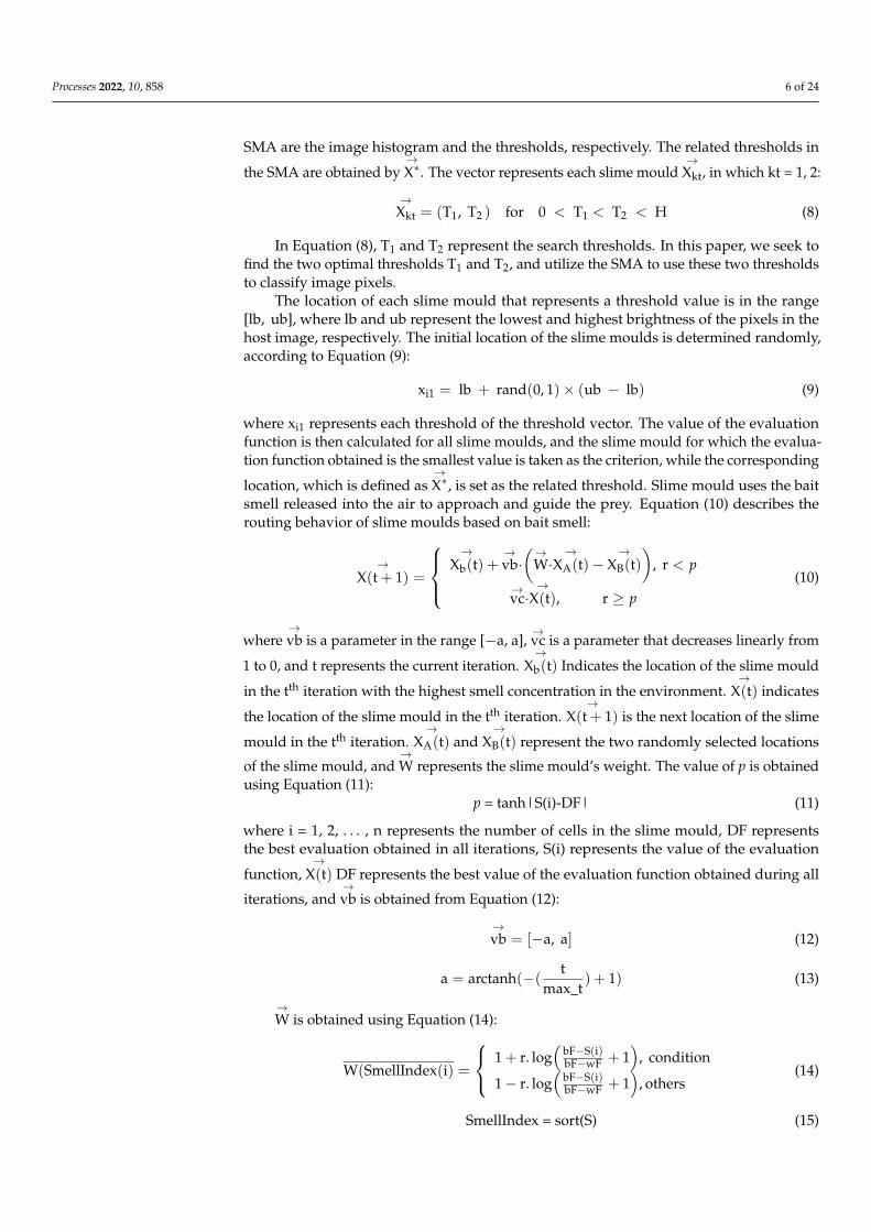
SMA are the image histogram and the thresholds, respectively. The related thresholds in

the SMA are obtained by→X∗. The vector represents each slime mould

→Xkt, in which kt = 1, 2:

→Xkt = (T1, T2 ) for 0 < T1 < T2 < H (8)

In Equation (8), T1 and T2 represent the search thresholds. In this paper, we seek tofind the two optimal thresholds T1 and T2, and utilize the SMA to use these two thresholdsto classify image pixels.

The location of each slime mould that represents a threshold value is in the range[lb, ub], where lb and ub represent the lowest and highest brightness of the pixels in thehost image, respectively. The initial location of the slime moulds is determined randomly,according to Equation (9):

xi1 = lb + rand(0, 1)× (ub − lb) (9)

where xi1 represents each threshold of the threshold vector. The value of the evaluationfunction is then calculated for all slime moulds, and the slime mould for which the evalua-tion function obtained is the smallest value is taken as the criterion, while the corresponding

location, which is defined as→X∗, is set as the related threshold. Slime mould uses the bait

smell released into the air to approach and guide the prey. Equation (10) describes therouting behavior of slime moulds based on bait smell:

→X(t + 1) =

→

Xb(t) +→vb·(→

W·→

XA(t)−→

XB(t))

, r < p

→vc·

→X(t), r ≥ p

(10)

where→vb is a parameter in the range [−a, a],

→vc is a parameter that decreases linearly from

1 to 0, and t represents the current iteration.→

Xb(t) Indicates the location of the slime mould

in the tth iteration with the highest smell concentration in the environment.→

X(t) indicates

the location of the slime mould in the tth iteration.→

X(t + 1) is the next location of the slime

mould in the tth iteration.→

XA(t) and→

XB(t) represent the two randomly selected locations

of the slime mould, and→W represents the slime mould’s weight. The value of p is obtained

using Equation (11):p = tanh|S(i)-DF| (11)

where i = 1, 2, . . . , n represents the number of cells in the slime mould, DF representsthe best evaluation obtained in all iterations, S(i) represents the value of the evaluation

function,→

X(t) DF represents the best value of the evaluation function obtained during all

iterations, and→vb is obtained from Equation (12):

→vb = [−a, a] (12)

a = arctanh(−( tmax_t

) + 1) (13)

→W is obtained using Equation (14):

W(SmellIndex(i) =

1 + r. log(

bF−S(i)bF−wF + 1

), condition

1− r. log(

bF−S(i)bF−wF + 1

), others

(14)

SmellIndex = sort(S) (15)

Processes 2022, 10, 858 7 of 24

The condition indicates that S(i) is in the first half of the population. The r representsa random value [0, 1]. The bF represents the value of the obtained optimal evaluationfunction in the current iteration. The wF represents the worst evaluation function receivedin the current iteration. SmellIndex represents the sequence of values of the evaluatedfunction (in ascending order). The location of the slime mould is also updated usingEquation (16) [36]:

→X∗=

rand.(UB− LB) + LB, rand < z→

Xb(t) +→vb.(

W.→

XA(t)−→

XB(t))

, r < p

→vc.

→X(t), r ≥ p

(16)

where LB and UB are the lower limit and the upper limit, respectively, which in this caseare equal to 0 and 255, respectively; rand and r are randomly determined in the range [0, 1],and the value of z will be discussed in the parameter setting test. Therefore, this process isrepeated until the stop condition is met. We set the stop condition to reach 100 iterations.

Then, we obtain the output→X∗, which represents the optimal threshold vector. Finally, the

host gray image A is divided into three separate classes C1, C2, and C3 using the optimalthresholds Tkt (kt = 1, 2), as shown in Equation (17):

C1 = {g(i, j) ∈ A| 0 ≤ g(i, j) ≤ T1 − 1}C2 = {g(i, j) ∈ A| T1 ≤ g(i, j) ≤ T2 − 1}C3 = {g(i, j) ∈ A| T2 ≤ g(i, j) ≤ H}

(17)

where g(i, j) represents each pixel in row i and column j of image A, and H representsthe gray area of gray image A. Thresholds Tkt are obtained by maximizing the evaluationfunction F, as shown in Equation (18):

Tkt = MAXTkt F(Tkt) (18)

where F(Tkt) is the same evaluation function for the SMA or the Otsu evaluation function.The Otsu evaluation function is calculated using Equation (19) [28]:

F = ∑ 2i=0SUMi(µi − µ1)

2 (19)

SUMi = ∑ Ti+1−1j=Ti

Pj (20)

µi = ∑ Ti+1−1j=Ti

iPj

SUMi, Pj = fer(j)/Nump (21)

In Equation (19), µ1 is the average density of the host image A for T1 = 0 andT2 = H. The µi is the average density of the Cy class for T1 and T2, and SUMi is thesum of the probabilities. In Equations (20) and (21), Pj shows the probability of the graylevel jth, fer(j) is the frequency of the jth gray level, and Nump represents the total numberof pixels in the host image A [36].

2.2. Data Insertion Process

In this paper, the value of 0 difference is also expanded for inserting the data (0 ≤ Th≤ 32) to increase the capacity, in addition to the fewer equal to 0 and fewer equal to 32differences [3]. In this paper, two optimal thresholds T1 and T2 are obtained for the hostimage, and the host image pixels are located together in three separate classes based on thetwo corresponding thresholds. Therefore, there is more similarity and correlation betweenthe pixels of each class, and the difference between two consecutive pixels related to eachclass is less.

By reducing the value of differences between consecutive pixels in each class, lessdistortion is created in the image due to data insertion based on the expansion of the value

Processes 2022, 10, 858 8 of 24

of differences. Furthermore, the capacity increases when increasing the number of pixelswith less difference between them.

After determining the optimal thresholds by the SMA, based on the two thresholds ofT1 and T2, starting from the pixel on the first row and the first column of the host image,pixels belonging to the first class—whose value is smaller than the threshold of T1—arelocated in the liner matrix C1. The second-class pixels, whose value is larger than that ofT1 and smaller than that of T2, are located in the liner matrix C2. Eventually, the pixelsbelonging to the third class, whose value is larger than that of T2—are located in the linermatrix C3. Figure 2 shows the status of the three matrices of C1, C2, and C3.

Processes 2022, 10, x FOR PEER REVIEW 8 of 24

Figure 2. Production of the matrices for three classes: (a) Class C1; (b) Class C2; (c) Class C3.

To insert the data, after classifications of host image pixels, matrix pixels Cy (y = 1, 2,

3) are divided into non-overlapping blocks with a size of 1 × 5. The vector P is then created

for pixels of each block to calculate the different values for both consecutive pixels, ac-

cording to Figure 3.

Figure 3. Production of the vector P.

According to Equation (22), differences are calculated for both consecutive pixels in

the vector P:

{

v1 = pCy,2 − pCy,1v2 = pCy,3 − pCy,2v3 = pCy,4 − pCy,3v4 = pCy,5 − pCy,4

(22)

Given that the proposed method inserts the data by expanding the value of differ-

ences to reduce distortion in the marked image, the blocks are selected to insert the data.

The difference between two consecutive pixels is between 0 and +32 (0 ≤ Th ≤ 32). Moreo-

ver, to reduce distortion in the marked image and the overflow/underflow control, the

range of each difference vk′(k′ = 1, 2, 3, 4) is diminished. A location map Mq (q = 1, 2, 3,

4) is created in each insertion layer to determine the locations of blocks inserted with data

bits. If the block is inserted with data bits, it will be equal to 1. Otherwise, it is equal to 0.

Furthermore, a location map LMy to separate each of the differences as 2 ≤ vk′ ≤ 32 or 0

≤ vk′ ≤ 1 is considered, as shown in Equation (23):

LMy = {0, if 0 ≤ vk′ ≤ 1

1, if 2 ≤ vk′ ≤ 32 (23)

If 0≤ vk′ ≤ 1, Equation (24) can be used to change the range of vk′:

vk′′ = |vk′ + 2| − 2

⌊log2(|vk′|)⌋ (24)

If 2≤ vk′ ≤ 32, Equation (25) can be used to change the range of vk′:

vk′′ = {

|vk′| − 2⌊log2(|vk′|)⌋−1, if 2 × 2n−1 ≤ |vk′| ≤ 3 × 2

n−1 − 1

|vk′| − 2⌊log2(|vk′|)⌋, if 3 × 2n−1 ≤ |vk′| ≤ 4 × 2

n−1 − 1 (25)

where n is calculated using Equation (26):

n = ⌊log2(|vk′|)⌋ (26)

Figure 2. Production of the matrices for three classes: (a) Class C1; (b) Class C2; (c) Class C3.

To insert the data, after classifications of host image pixels, matrix pixels Cy (y = 1,2, 3) are divided into non-overlapping blocks with a size of 1 × 5. The vector P is thencreated for pixels of each block to calculate the different values for both consecutive pixels,according to Figure 3.

Processes 2022, 10, x FOR PEER REVIEW 8 of 24

Figure 2. Production of the matrices for three classes: (a) Class C1; (b) Class C2; (c) Class C3.

To insert the data, after classifications of host image pixels, matrix pixels Cy (y = 1, 2,

3) are divided into non-overlapping blocks with a size of 1 × 5. The vector P is then created

for pixels of each block to calculate the different values for both consecutive pixels, ac-

cording to Figure 3.

Figure 3. Production of the vector P.

According to Equation (22), differences are calculated for both consecutive pixels in

the vector P:

{

v1 = pCy,2 − pCy,1v2 = pCy,3 − pCy,2v3 = pCy,4 − pCy,3v4 = pCy,5 − pCy,4

(22)

Given that the proposed method inserts the data by expanding the value of differ-

ences to reduce distortion in the marked image, the blocks are selected to insert the data.

The difference between two consecutive pixels is between 0 and +32 (0 ≤ Th ≤ 32). Moreo-

ver, to reduce distortion in the marked image and the overflow/underflow control, the

range of each difference vk′(k′ = 1, 2, 3, 4) is diminished. A location map Mq (q = 1, 2, 3,

4) is created in each insertion layer to determine the locations of blocks inserted with data

bits. If the block is inserted with data bits, it will be equal to 1. Otherwise, it is equal to 0.

Furthermore, a location map LMy to separate each of the differences as 2 ≤ vk′ ≤ 32 or 0

≤ vk′ ≤ 1 is considered, as shown in Equation (23):

LMy = {0, if 0 ≤ vk′ ≤ 1

1, if 2 ≤ vk′ ≤ 32 (23)

If 0≤ vk′ ≤ 1, Equation (24) can be used to change the range of vk′:

vk′′ = |vk′ + 2| − 2

⌊log2(|vk′|)⌋ (24)

If 2≤ vk′ ≤ 32, Equation (25) can be used to change the range of vk′:

vk′′ = {

|vk′| − 2⌊log2(|vk′|)⌋−1, if 2 × 2n−1 ≤ |vk′| ≤ 3 × 2

n−1 − 1

|vk′| − 2⌊log2(|vk′|)⌋, if 3 × 2n−1 ≤ |vk′| ≤ 4 × 2

n−1 − 1 (25)

where n is calculated using Equation (26):

n = ⌊log2(|vk′|)⌋ (26)

Figure 3. Production of the vector P.

According to Equation (22), differences are calculated for both consecutive pixels inthe vector P:

v1 = pCy,2− pCy,1

v2 = pCy,3− pCy,2

v3 = pCy,4− pCy,3

v4 = pCy,5− pCy,4

(22)

Given that the proposed method inserts the data by expanding the value of differencesto reduce distortion in the marked image, the blocks are selected to insert the data. Thedifference between two consecutive pixels is between 0 and +32 (0 ≤ Th ≤ 32). Moreover,to reduce distortion in the marked image and the overflow/underflow control, the rangeof each difference vk′

(k′ = 1, 2, 3, 4

)is diminished. A location map Mq (q = 1, 2, 3, 4) is

created in each insertion layer to determine the locations of blocks inserted with data bits.If the block is inserted with data bits, it Mq will be equal to 1. Otherwise, it is equal to0. Furthermore, a location map LMy to separate each of the differences as 2 ≤ vk′ ≤ 32or 0 ≤ vk′ ≤ 1 is considered, as shown in Equation (23):

LMy =

{0, if 0 ≤ vk′ ≤ 11, if 2 ≤ vk′ ≤ 32

(23)

Processes 2022, 10, 858 9 of 24

If 0≤ vk′ ≤ 1, Equation (24) can be used to change the range of vk′ :

v′k′ = |vk′ + 2| − 2blog2 (|vk′ |)c (24)

If 2 ≤ vk′ ≤ 32, Equation (25) can be used to change the range of vk′ :

v′k′ =

{|vk′ | − 2blog2 (|vk′ |)c−1, if 2× 2n−1 ≤ |vk′ | ≤ 3× 2n−1 − 1|vk′ | − 2blog2 (|vk′ |)c, if 3× 2n−1 ≤ |vk′ | ≤ 4× 2n−1 − 1

(25)

where n is calculated using Equation (26):

n = blog2(|vk′ |)c (26)

In each insertion layer of each y class, a location map LM′y,f—where f = 1, 2, as shownin Equations (27) and (28)—is used to recover the original differences. LM′y,1 and LM′y,2are used to separate the differences, as 0 ≤ vk′ ≤ 1 and 2 ≤ vk′ ≤ 32, respectively.

LM′y,1 =

{0, if |vk′ | = 01, if |vk′ | = 1

(27)

LM′y,2 =

{0, if 2× 2n−1 ≤ |vk′ | ≤ 3× 2n−1 − 11, if 3× 2n−1 ≤ |vk′ | ≤ 4× 2n−1 − 1

(28)

The matrices Mq ‘LMy, and LM′y,f are used to recover the original differences andoriginal image pixels. Given that in the proposed method, in the sth insertion layer(s = 1, 2, 3, 4, 5), the sth pixel is not inserted for reversibility, and in each layer, four -bits of data are inserted in four pixels of each block, the data bits’ sequence is divided into4-bit subsequences, where bk′ = (b1, b2, b3, b4)2 that k′ = 1, 2, 3, 4. Then, using Equation(29), v′k′ expands with a datum:

v′′k′= 2× v′k′ + bk′ (29)

The first pixel is not inserted from each block in the first layer. Therefore, in the firstinsertion layer, insertion of the 4-bit sequence b in pixels of each block is carried out asshown in Equation (30). In the second insertion layer, the second pixels of each class blockare not selected to insert the data. In this layer, the process of inserting the 4-bit sequence bin pixels of each block is as shown in Equation (31). In the third insertion layer, the thirdpixel of each class block is not selected to insert the data, according to Equation (32). Inthe 4th insertion layer, the 4th pixel of each class block is not selected to insert the data,according to Equation (33).

pCy,1′ = PCy,1

pCy,2′ = v′′1 + PCy,1

pCy,3′ = v′′2 + pCy,2

pCy,4′ = v′′3 + pCy,3

pCy,5′ = v′′4 + pCy,4

(30)

pCy,1′ = v′′1 + PCy,1

pCy,2′ = PCy,2

pCy,3′ = v′′2 + pCy,2

pCy,4′ = v′′3 + pCy,3

pCy,5′ = v′′4 + pCy,4

(31)

Processes 2022, 10, 858 10 of 24

pCy,1′ = v′′1 + PCy,1

pCy,2′ = v′′2 + PCy,2

pCy,3′ = pCy,2

pCy,4′ = v′′3 + pCy,3

pCy,5′ = v′′4 + pCy,4

(32)

pCy,1′ = v′′1 + PCy,1

pCy,2′ = v′′2 + PCy,2

pCy,3′ = v′′3 + pCy,2

pCy,4′ = pCy,3

pCy,5′ = v′′4 + pCy,4

(33)

Therefore, due to the data insertion process of pixels pCy,1, pCy,2

, pCy,3, pCy,4

and pCy,5

from each block, five marked pixels p′Cy,1, p′Cy,2

, p′Cy,3, p′Cy,4

, and p′Cy,5are obtained, as is

the marked image A′.The steps of the data insertion process in each insertion layer are as follows:Step 1: Dividing the data sequence into 4-bit b. Step 2: Apply SMA on the host image

to determine the optimal thresholds T1 and T2. Step 3: Classification of image pixels basedon thresholds T1 and T2. Step 4: Dividing the class pixels Cy into non-overlapping blocksof size 1 × 5. Step 5: Production of a location map Mq to determine the block locations withinsertion conditions. Step 6: Produce the vector P for each selected block to calculate thevalue of differences. Step 7: Calculate the differences vk′ for both consecutive pixels, andthen calculate v′k′ . Step 8: Calculate the value of v′′

k′to reduce image distortion and prevent

overflow/underflow. Step 9: Produce the location map LMy. Step 10: Calculation of themarked pixels p′Cy,1

, p′Cy,2, p′Cy,3

, p′Cy,4, and p′Cy,5

. Step 11: Produce the marked image

A′ and save the location maps LMy, LM′y,f, and Mq, and thresholds T1 and T2 in order toextract the original data and recover the original image.

2.3. Data Extraction Process

In the extraction phase, the marked image A′ is first classified using the thresholdsT1 and T2, and the pixels belonging to each class are located in the matrix C′y. Then, thepixels belonging to the matrix C′y are divided into blocks of size 1 × 5, and using locationmaps the LMy and LM′y,f the secret data are extracted from the corresponding blocks, andthe original image pixels are recovered. The extraction process is performed from the firstinsertion to the last. The vector p′ is created for the pixels of each block after dividing thematrix C′y into blocks of size 1 × 5, according to Equation (34):

p′ =(

p′Cy,1, p′Cy,2

, p′Cy,3, p′Cy,4

, p′Cy,5

)(34)

In each insertion layer, the binary value v′′k′

is obtained. Then, the least significant bit(LSB) of v′′

k′as the k′th bit is extracted from the secret data. In the 4th insertion layer, extract-

ing the data bits bk′ and recovering the original pixels from each vector p′ is performed asfollows (see Equations (35)–(38)):

v′′1 = P′Cy,k′− P′Cy,k′

(35)

bk′ = LSB(v′′k′) (36)

vk′′ =

⌊v′′

k′

2

⌋(37)

P′Cy,k′= P′Cy,k′−1

+ vk′−1 (38)

Processes 2022, 10, 858 11 of 24

If the LM′y,1 is equal to 0 or 1, Equation (39) can be used to obtain vk′ . If the LM′y,2 isequal to 0 or 1, Equation (40) can be used to obtain vk′ .

vk′ =∣∣v′k′ ∣∣− 2blog2 (|vk′ |)c (39)

vk′ =

∣∣∣v′k′ ∣∣∣+ 2blog2 (|vk′ |)c, if LM′y, 2 = 0∣∣∣v′k′ ∣∣∣+ 2blog2 (|vk′ |)c, if LM′y,2 = 1

(40)

The values of pCy,1pCy,2

, b1, and v1′ are obtained using Equations (41)–(57).

Pcy,1 = P′cy,1(41)

v′′1 = P′Cy,2− Pcy,1 (42)

b1 = LSB(v′′1)

(43)

v1′ =

⌊v′′12

⌋(44)

Pcy,2 = Pcy,1 + v1 (45)

Therefore, the value v1 is obtained using Equation (39) or Equation (40). Then, pCy,3,

b2, and v2′ are obtained using the following equations:

v′′2 = P′Cy,3− Pcy,2 (46)

b2 = LSB(v′′2)

(47)

v2′ =

⌊v′′22

⌋(48)

Pcy,3 = Pcy,2 + v2 (49)

Therefore, the value v2 is obtained using Equation (39) or Equation (40).Then, pCy,4

, b3, and v3′ are obtained using the following equations:

v′′3 = P′Cy,4− Pcy,3 (50)

b3 = LSB(v′′3)

(51)

v3′ =

⌊v′′32

⌋(52)

Pcy,4 = Pcy,3 + v3 (53)

Therefore, the value v3 is obtained using Equations (39) and (40).Then, pCy,5

, b4, and v4′ are obtained using the following equations:

v′′4 = P′Cy,5− Pcy,4 (54)

b4 = LSB(v′′4)

(55)

v4′ =

⌊v′′42

⌋(56)

Pcy,5 = Pcy,4 + v4 (57)

Therefore, the value v4 is obtained using Equations (39) and (40).

Processes 2022, 10, 858 12 of 24

The steps of the data extraction process and the original host image pixel recovery ineach layer are as follows:

Step 1: Classify the pixels of the image A′ to get three classes Cy.Step 2: Dividing the class pixels Cy into non-overlapping blocks of size 1 × 5.Step 3: Identify marked blocks using the location map Mq.Step 4: Production of the vector p′ for each block.Step 5: Calculate the value v′′

k′.

Step 6: Extract the inserted data bk′ using the first LSB v′′k′

.Step 7: Calculate the value vk′

′.Step 8: Calculate the value of the vk′ difference using LMy and LM′y,f.Step 9: Calculate the original pixels of each block.Step 10: Recover the original image A.The marked pixels in the respective block are shown in Figure 4. An example of the

embedding and extraction process:

Processes 2022, 10, x FOR PEER REVIEW 12 of 24

Figure 4. An example of quad-pixel reversible data embedding: (a) before embedding; (b) after em-

bedding; (c) after extraction.

Embedding process:

P = (106, 121, 148, 158, 155)

{

𝑣1 = 121 − 106 = 15𝑣2 = 148 − 121 = 27𝑣3 = 158 − 148 = 10𝑣4 = 158 − 158 = 0

𝑣𝑘′ = (15, 27, 10, 0), b=(0, 1, 1, 0)

𝑣1 = 15, 𝑛 = 3, 𝑣1′′ = 7, 𝐿𝑀′

𝑦,2 = 1, 𝑏1 = 0, 𝑣1″ = 2 × 7 + 0 = 14

𝑣2 = 27, n = 4, 𝑣2′′ = 11, 𝐿𝑀′

𝑦,2 = 1, 𝑏2 = 1, 𝑣2″ = 2 × 11 + 1 = 23

𝑣3 = 10, n = 4, 𝑣3′′ = 6, 𝐿𝑀′

𝑦,2 = 0, 𝑏3 = 1, 𝑣3″ = 2 × 6 + 1 = 13

𝑣4 = 0, n = 4, 𝑣4′′ = 1, 𝐿𝑀′

𝑦,1 = 1, 𝑏4 = 0, 𝑣4″ = 2 × 1 + 0 = 2

𝑣𝑘′′ = (7, 11, 6, 1), 𝑣𝑘′

″ = (14, 55, 13, 2), 𝐿𝑀′𝑦,2 = (1, 1, 0)2, M = 1

{

𝑝1′ = 106

𝑝2′ = 106 + 14 = 120

𝑝3′ = 121 + 23 = 144

𝑝4′ = 148 + 13 = 161

𝑝5′ = 158 + 2 = 160

𝑝′ = (106, 120, 144, 161, 160)

Extraction process:

𝑝′ = (106, 120, 144, 161, 160)

𝑣1″ = 120 − 106 = 14

𝑏1 = LSB(14) =𝐿𝑆𝐵(1110)2 = 0

𝑣1′ = ⌊

14

2⌋ = 7

𝐿𝑀′𝑦,1 = 1, 𝑣1 = 15

{𝑝𝐶𝑦,1 = 106

𝑝𝐶𝑦,2 = 106 + 15 = 121

𝑣2″ = 144 − 121 = 23

𝑏2 = LSB(23) = 𝐿𝑆𝐵(10111)2 = 1

Figure 4. An example of quad-pixel reversible data embedding: (a) before embedding; (b) afterembedding; (c) after extraction.

Embedding process:

P = (106, 121, 148, 158, 155)v1 = 121− 106 = 15v2 = 148− 121 = 27v3 = 158− 148 = 10v4 = 158− 158 = 0

vk′ = (15, 27, 10, 0), b = (0, 1, 1, 0)v1 = 15, n = 3, v′1′ = 7, LM′y,2 = 1, b1 = 0, v′′1= 2× 7 + 0 = 14v2 = 27, n = 4, v′2′ = 11, LM′y,2 = 1, b2 = 1, v′′2= 2× 11 + 1 = 23v3 = 10, n = 4, v′3′ = 6, LM′y,2 = 0, b3 = 1, v′′3= 2× 6 + 1 = 13v4 = 0, n = 4, v′0′ = 1, LM′y,2 = 1, b4 = 0, v′′4= 2× 1 + 0 = 2v′k′ = (7, 11, 6, 1), v′′k′ = (14, 55, 13, 2), LM′y,2 = (1, 1, 0)2, M = 1

p1′ = 106

p2′ = 106 + 14 = 120

p3′ = 121 + 23 = 144

p4′ = 148 + 13 = 161

p5′ = 158 + 2 = 160

p′(106, 120, 144, 161, 160)

Processes 2022, 10, 858 13 of 24

Extraction process:

p′(106, 120, 144, 161, 160)v′′1 = 120− 106 = 14b1 =LSB(14) = LSB(1110)2 = 0v1′ =

⌊142

⌋= 7

LM′y,1 = 1, v1 = 15{pCy,1 = 106pCy,2 = 106 + 15 = 121

v′′2 = 144− 121 = 23b2 = LSB(23) = LSB(10111)2 = 2v2′ =

⌊ 232⌋= 11

LM′y,2 = 1, v2 = 27pCy,3 = 27 + 121 = 148v′′3 = 161− 148 = 13b3 = LSB(13) = LSB(1101 )2 = 1v3′ =

⌊132

⌋= 6

LM′y,2 = 0, v3 = 10pCy,4 = 148 + 10 = 158v′′4 = 160− 158 = 2b4 = LSB(2) = LSB(10 )2 = 0v3′ =

⌊ 22⌋= 1

LM′y,1 = 1, v3 = 0pCy,5 = 158 + 0 = 158

Finally, the initial pixels of the corresponding block are retrieved as follows.

P = (106, 121, 148, 158, 155)

3. Results

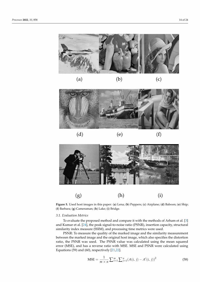
In this paper, the gray images of Lena, Peppers, Airplane, Baboon, Ship, Lake, Bridge,Cameraman, and Barbara are used as the host image of size 512 × 512, taken from theUSC-SIPI database. Figure 5 shows the host images used in this paper. The proposedmethod is simulated using MATLAB 2018b and a Windows 64-bit operating system with aCore i5 CPU.

Processes 2022, 10, 858 14 of 24Processes 2022, 10, x FOR PEER REVIEW 14 of 24

Figure 5. Used host images in this paper: (a) Lena; (b) Peppers; (c) Airplane; (d) Ba-

boon; (e) Ship; (f) Barbara; (g) Cameraman; (h) Lake; (i) Bridge.

3.1. Evaluation Metrics

To evaluate the proposed method and compare it with the methods of Arham et al.

[3] and Kumar et al. [24], the peak signal-to-noise ratio (PSNR), insertion capacity, struc-

tural similarity index measure (SSIM), and processing time metrics were used.

PSNR: To measure the quality of the marked image and the similarity measurement

between the marked image and the original host image, which also specifies the distortion

ratio, the PSNR was used. The PSNR value was calculated using the mean squared error

(MSE), and has a reverse ratio with MSE. MSE and PSNR were calculated using Equations

(59) and (60), respectively [21,22].

MSE = 1

𝑚×𝑛∑ ∑ (𝐴(𝑖, 𝑗) − 𝐴′(𝑖, 𝑗)𝑛

𝑗=1𝑚𝑖=1 )2 (58)

PSNR = 10𝐿𝑜𝑔10(2552

𝑀𝑆𝐸) (59)

For the image with a size of m × n, A (i, j) represents the host image pixels, and 𝐴′(𝑖, 𝑗)

represents the marked image pixels.

Figure 5. Used host images in this paper: (a) Lena; (b) Peppers; (c) Airplane; (d) Baboon; (e) Ship;(f) Barbara; (g) Cameraman; (h) Lake; (i) Bridge.

3.1. Evaluation Metrics

To evaluate the proposed method and compare it with the methods of Arham et al. [3]and Kumar et al. [24], the peak signal-to-noise ratio (PSNR), insertion capacity, structuralsimilarity index measure (SSIM), and processing time metrics were used.

PSNR: To measure the quality of the marked image and the similarity measurementbetween the marked image and the original host image, which also specifies the distortionratio, the PSNR was used. The PSNR value was calculated using the mean squarederror (MSE), and has a reverse ratio with MSE. MSE and PSNR were calculated usingEquations (59) and (60), respectively [21,22].

MSE =1

m× n ∑ mi=1 ∑ n

j=1(A(i, j)− A′(i, j))2 (58)

Processes 2022, 10, 858 15 of 24

PSNR = 10Log10(2552

MSE) (59)

For the image with a size of m× n, A (i, j) represents the host image pixels, and A′(i, j)represents the marked image pixels.

Insertion capacity: This paper used a random bit sequence as secret data. For a grayhost image with a size of m × n, the maximum insertion capacity was calculated accordingto the number of bits per pixel (bpp), using Equation (61) [3]:

Insertion capacity(bpp) =Length o f sequence bit

m× n(60)

In the proposed method, the multilayer insertion technique enhances the capacity.Arham et al. [3] considered the maximum number of insertion layers to be eight. Therefore,the data insertion process was performed two times, and at each time, data bits wereinserted under four layers—the first time from the first layer to the fourth layer, and thesecond time from the fifth layer to the eighth layer.

SSIM: The SSIM metric is a famous metric used to measure the amount of structuralsimilarity between the host image A and image A′. This metric can be obtained usingEquation (62) [34]:

SSIM(A, A′) =(2µ1µA′ + c1)(2σ1,A′ + c2)

(µ21 + µ2

A′ + c1)(σ11 + σ2

A′ + c2)(61)

where µ1 and µA′ are the mean brightness intensity of A and A′, respectively, σA′ repre-sents the standard deviation of images A and A′, respectively, σ1,A′ represents covariancebetween images A and A′, respectively, and c1 and c2 are two constant values of 6.50 and58.52, respectively. The higher the SSIM value in data hiding methods and the closer it is to1, the more effective the corresponding process [34].

Processing time: processing time is one of the essential parameters for comparisonto DH methods. Therefore, the total processing time is equal to the total insertion andextraction time values to compare the proposed method and other methods.

3.2. Comparison with the Other Methods

In this paper, the proposed method is compared with the methods of Arham et al. [3],Yao et al. [22], and Kumar et al. [16]. Similarity and correlation between pixels belonging toeach class are increased using multilevel thresholding, and the difference between the pixelsdecreases. As a result, inserting a few layers of data creates less distortion in the image.

Because, in the proposed method, all of the values of zero and positive differences areexpanded to insert the data, in the first insertion layer and higher insertion layers, it has ahigher insertion capacity and PSNR than the methods of Arham et al. [3], Yao et al. [30],and Kumar et al. [24]. As a result, the resulting distortion in the marked image for theproposed method is less than that in the methods of Arham et al. [3], Yao et al. [30], andKumar et al. [24]. Table 2 shows the values of insertion capacity maxima for differentimages per thresholds T1 and T2 at 0 ≤ Th ≤ +32. The values of T1 and T2 are set bythe SMA. Table 3 shows the values of processing time (seconds) for different images perthresholds T1 and T2 at 0 ≤ Th ≤ +32.

As can be seen from Tables 2 and 3, for the two thresholds and T2 in the first insertionlayer, the proposed method has more insertion capacity and more PSNR for all images thanthe methods of Arham et al. [3] and Kumar et al. [24].

According to Table 2, the insertion capacity of the first insertion layer in the proposedmethod for the Airplane, Baboon, Barbara, Ship, Lena, Lake, Bridge, Cameraman, andPeppers images is 834 bits (0.0032 bpp), 1689 bits (0.0064 bpp), 766 bits (0.0029 bpp), 1561bits (0.0059 bpp), 2241 bits (0.0085 bpp), 1604 bits (0.0061 bpp), 4402 bits (0.0168 bpp), 4794bits (0.0183 bpp), and 1571 bits (0.0061 bpp), respectively—more than in the method ofArham et al. [3].

Processes 2022, 10, 858 16 of 24

Table 2. A comparison of the actual embedding capacities in common images.

Proposed Insertion Capacity (bits) Insertion Capacity (bpp)

Image T1 T2 [3] [24] PM [3] [24] PM

Airplane 111 182 194,250 210,000 215,000 0.7449 0.8010 0.8201Baboon 78 149 193,314 110,000 195,003 0.7374 0.4196 0.7438Barbara 55 131 191,466 158,000 192,232 0.7304 0.6027 0.7333Ship 79 156 194,583 160,000 196,144 0.7423 0.6103 0.7482Lena 85 152 196,768 200,000 209,000 0.7480 0.7629 0.7972Lake 76 145 191,854 111,000 193,458 0.7318 0.4234 0.7514Bridge 84 151 192,472 185,000 196,874 0.7342 0.7186 0.7379Cameraman 91 174 194,968 159,000 199,762 0.7437 0.6039 0.7510Peppers 61 136 195,414 178,000 196,985 0.7454 0.6790 0.7514

PM = proposed method.

Table 3. A comparison of the processing times in common images.

Proposed Processing Time (s)

Image T1 T2 [3] [24] PM

Airplane 111 182 154.09 1.29 173.94Baboon 78 149 153.72 1.81 173.60Barbara 55 131 151.44 1.37 175.35Ship 79 156 138.11 1.44 160.99Lena 85 152 153.58 1.67 181.56Lake 76 145 152.41 1.37 174.56Bridge 84 151 153.25 1.41 175.92Cameraman 91 174 139.48 1.62 179.45Peppers 61 136 154.11 1.15 185.98

PM = proposed method.

In the proposed method, the Lena image has the highest increase in capacity (0.0085bpp), while the Barbara image has the lowest increase in capacity (0.0029 bpp), comparedto the method of Arham et al. [3]. Therefore, on average, the capacity of the first insertionlayer in the proposed method is 0.0058 bpp more than that of the method of Arham et al. [3].The average processing time for the proposed method is 173.2367 s, while that for themethod of Arham et al. [3] is 150.8417 s. Therefore, the proposed method is slower thanthe method of Arham et al. [3], due to the use of the SMA and its repetitions to obtainoptimal thresholds.

Moreover, the proposed method is better than the method of Kumar et al. [24] in termsof PSNR and embedding capacity values, as can be seen in Tables 2 and 3, but in terms ofexecution time it is slower compared to the methods of Kumar et al. [24] and Arham et al. [3].Furthermore, the proposed method, compared to the method of Kumar et al. [24] for theLake, Bridge, Cameraman, Airplane, Baboon, Barbara, Ship, Lena, and Peppers images,yields 82,485 bits (3145 bpp), 11,874 bits (0.0324 bpp), 40,762 bits (0.1581 bpp), 5000 bits(0.0191 bpp), 85,000 bits (0.3242 bpp), 34,232 bits (0.1306 bpp), 36,144 bits (0.1379 bpp), 9000bits (0.0343 bpp) and 18,985 bits (0.0724 bpp), respectively, showing greater capacity.

Table 4 also compares the PSNR values of the proposed method with the methodof Arham et al. [3] for different capacities of 0.1 bpp, 0.2 bpp, 0.3 bpp, 0.4 bpp, 0.5 bpp,0.6 bpp, and 0.7 bpp in the first insertion layer. As can be seen from Table 4, the averagePSNR of the proposed method for different capacities is higher than that of the method ofArham et al. [3].

Processes 2022, 10, 858 17 of 24

Table 4. Comparison of the PSNR (dB) value single-layer embedding in terms of visual qualitytest images.

PSNR (dB)

0.1 bpp 0.2 bpp 0.3 bpp 0.4 bpp 0.5 bpp 0.6 bpp 0.7 bpp

Airplane [3] 54.35 51.88 48.85 44.36 42.45 41.44 40.92Proposed 55.17 52.73 49.99 45.40 44.07 43.11 41.86

Baboon[3] 40.95 38.97 37.98 36.95 36.48 35.97 35.40

Proposed 42.01 40.03 38.88 37.34 37.11 36.54 36.89

Barbara[3] 49.29 46.73 43.84 41.12 38.98 37.50 36.57

Proposed 50.74 47.43 44.45 42.31 39.12 38.61 37.63

Ship [3] 50.71 46.86 43.85 41.95 40.92 40.46 40.19Proposed 51.85 48.46 45.48 43.01 42.15 41.64 41.78

Lena[3] 54.70 50.31 47.74 45.77 44.19 43.03 42.16

Proposed 55.18 52.12 48.61 46.17 45.46 44.61 43.44

Lake[3] 48.32 44.16 40.35 38.36 36.56 34.79 33.21

Proposed 49.97 45.98 41.68 39.86 37.15 35.96 34.56

Bridge [3] 47.76 43.32 39.86 36.75 34.85 33.45 31.99Proposed 49.23 44.53 40.96 37.82 35.98 34.59 32.68

Cameraman[3] 46.12 42.36 38.25 34.91 32.56 31.20 30.05

Proposed 48.06 43.74 39.94 36.20 34.11 32.31 31.11

Peppers [3] 49.66 47.12 45.37 43.92 43.15 42.61 42.05Proposed 51.11 48.94 46.33 44.61 45.20 43.45 43.11

Figure 6 shows the PSNR comparison diagram of the proposed method with themethod of Arham et al. [3] for different images under the same capacities drawn using thedata shown in Tables 4 and 5. As can be seen from the diagrams in Figure 6, the proposedmethod has a higher PSNR value for all images than the method of Arham et al. [3]. Forthe first insertion layer, the Airplane image for the capacities of 0.1 bpp, 0.2 bpp, 0.3 bpp,0.4 bpp, 0.5 bpp, 0.6 bpp, and 0.7 bpp shows increases in quality compared to the methodof Arham et al. [3] of 0.8200 dB, 0.8500 dB, 1.1400 dB, 1.04 dB, 1.6200 dB, 1.6700 dB, and0.94 dB, respectively.

Table 5. A comparison of the PSNR (dB) value multiple-layer embedding in terms of visual qualitytest images.

PSNR (dB)

0.7 bpp 1.5 bpp 2.2 bpp 3 bpp 3.7 bpp 4.5 bpp 5.2 bpp 6 bpp

Airplane [3] 40.5 36.59 35.1 34 32.5 31.9 31 30Proposed 41.12 38.02 36.25 35.01 33.84 32.56 32.97 31.01

Baboon[3] 35.1 32 30 28.5 27.1 26.2 25.3 25

Proposed 36.98 33.24 31.12 29.95 28.87 27.97 26.78 26.25

Barbara[3] 36.2 33.9 32 30.7 29.1 28.83 27.8 27

Proposed 37.45 34.25 33.12 31.99 30.47 30.02 28.11 28

Ship [3] 40.58 36.9 35 33.2 32 31.57 30 29.1Proposed 42.01 37.2 36.11 34.42 33 33.03 31 30.25

Lena[3] 42 38.2 37 35.1 34 33 32.1 31.1

Proposed 43.52 39.44 38 36.55 35 34.11 33 32

Lake[3] 37.26 34.73 32.82 31.74 30.82 29 27.76 26

Proposed 38.99 35.47 34.15 33.26 32.42 30.76 29.12 27.22

Bridge [3] 37.85 33.72 32.25 31.74 29.18 28 26.87 25.10Proposed 39.23 35.28 33.76 32.06 30.46 29 27.75 26

Cameraman[3] 40.51 36.97 34.98 32.76 30.56 28.75 27 25.34

Proposed 42.07 38.13 36.46 35.36 32.89 31.46 29.42 26.12

Peppers [3] 41.9 38.3 36.3 35 34 33 32 31.1Proposed 43 39.85 37 36.55 35.89 34 33 32.34

Processes 2022, 10, 858 18 of 24

Processes 2022, 10, x FOR PEER REVIEW 18 of 24

Cameraman [3] 40.51 36.97 34.98 32.76 30.56 28.75 27 25.34

Proposed 42.07 38.13 36.46 35.36 32.89 31.46 29.42 26.12

Peppers [3] 41.9 38.3 36.3 35 34 33 32 31.1

Proposed 43 39.85 37 36.55 35.89 34 33 32.34

(a) (b)

(c) (d)

(e) (f)

Processes 2022, 10, x FOR PEER REVIEW 19 of 24

(g) (h)

Figure 6. Comparison of image quality for single-layer capacity: (a) Airplane; (b) Baboon; (c) Bar-

bara; (d) Ship; (e) Lena; (f) Peppers; (g) Lake; (h) Bridge [3].

Moreover, the Baboon image for the capacities of 0.1 bpp, 0.2 bpp, 0.3 bpp, 0.4 bpp,

0.5 bpp, 0.6 bpp, and 0.7 bpp, compared to the method of Arham et al. [3], shows increases

in quality of 1.0600 dB, 0.9600 dB, 0.9000 dB, 0.3900 dB, 0.6300 dB, 0.5700 dB and 1.4900

dB, respectively. Meanwhile, the Barbara image for the capacities of 0.1 bpp, 0.2 bpp, 0.3

bpp, 0.4 bpp, 0.5 bpp, 0.6 bpp, and 0.7 bpp increases in quality by 1.4500 dB, 0.7000 dB,

0.610.0 dB, 1.1900 dB, 0.1400 dB, 1.1100 dB, and 1.0600 dB, respectively, compared to the

method of Arham et al. [3].

The Ship image for the capacities of 0.1 bpp, 0.2 bpp, 0.3 bpp, 0.4 bpp, 0.5 bpp, 0.6

bpp, and 0.7 bpp increases in quality by 1.1400 dB, 1.6000 dB, 1.6300 dB, 1.0600 dB, 1.2300

dB, 1.1800 dB, and 1.5900 dB, respectively, compared to the method of Arham et al. [3].

The Lena image for capacities of 0.1 bpp, 0.2 bpp, 0.3 bpp, 0.4 bpp, 0.5 bpp, 0.6 bpp

and 0.7 bpp, compared to the method of Arham et al. [3], has an increase in quality of

0.4800 dB, 1.8100 dB, 0.8700 dB, 0.4000 dB, 1.2700 dB, 1.5800 dB, and 1.2800 dB, respec-

tively. The Peppers image for capacities of 0.1 bpp, 0.2 bpp, 0.3 bpp, 0.4 bpp, 0.5 bpp, 0.6

bpp, and 0.7 bpp, compared to the method of Arham et al. [3], has an increase in quality

of 1.6500 dB, 1.8200 dB, 1.3300 dB, 1.50 dB, 0.5900 dB, 1.1700 dB, and 1.3500 dB, respec-

tively. The Lake image for the capacities of 0.1 bpp, 0.2 bpp, 0.3 bpp, 0.4 bpp, 0.5 bpp, 0.6

bpp, and 0.7 bpp increases in quality by 1.4700 dB, 1.2100 dB, 1.1000 dB, 1.0700 dB, 1.1300

dB, 1.1400 dB, and 0.6900 dB, respectively, compared to the method of Arham et al. [3].

The Cameraman image for capacities of 0.1 bpp, 0.2 bpp, 0.3 bpp, 0.4 bpp, 0.5 bpp,

0.6 bpp and 0.7 bpp, compared to the method of Arham et al. [3], has an increase in quality

of 1.9400 dB, 1.3800 dB, 1.6900 dB, 1.2900 dB, 1.5500 dB, 1.1100 dB, and 1.0600 dB, respec-

tively. The Bridge image for capacities of 0.1 bpp, 0.2 bpp, 0.3 bpp, 0.4 bpp, 0.5 bpp, 0.6

bpp, and 0.7 bpp, compared to the method of Arham et al. [3], has an increase in quality

of 1.4500 dB, 1.8200 dB, 0.9600 dB, 1.2400 dB, 1.5000 dB, 0.8400 dB, and 1.0600 dB, respec-

tively.

The proposed method has more insertion capacity than that of Arham et al. [3] for

the first and higher insertion layers. Table 5 shows the PSNR comparison of the proposed

method and the method of Arham et al. [3] for the eight insertion layers. As the number

of insertion layers increases, the total insertion capacity increases. As shown in Table 5,

the values of insertion capacity and PSNR for the proposed method are higher than those

in the method of Arham et al. [3]. According to Table 5, the average insertion capacity

increase in the eight insertion layers in the proposed method is 0.625 bpp, and in the

method of Arham et al. [3] it is 0.572 bpp. In insertion layer eight, the Peppers, Lena, Bar-

bara, and Baboon images have the highest increase in capacity, while the Airplane, Ship,

Lake, Bridge, and Cameraman images have the slightest increase in capacity, compared

to the method of Arham et al. [3].

Figure 6. Comparison of image quality for single-layer capacity: (a) Airplane; (b) Baboon; (c) Barbara;(d) Ship; (e) Lena; (f) Peppers; (g) Lake; (h) Bridge [3].

Processes 2022, 10, 858 19 of 24

Moreover, the Baboon image for the capacities of 0.1 bpp, 0.2 bpp, 0.3 bpp, 0.4 bpp,0.5 bpp, 0.6 bpp, and 0.7 bpp, compared to the method of Arham et al. [3], shows increasesin quality of 1.0600 dB, 0.9600 dB, 0.9000 dB, 0.3900 dB, 0.6300 dB, 0.5700 dB and 1.4900 dB,respectively. Meanwhile, the Barbara image for the capacities of 0.1 bpp, 0.2 bpp, 0.3 bpp,0.4 bpp, 0.5 bpp, 0.6 bpp, and 0.7 bpp increases in quality by 1.4500 dB, 0.7000 dB, 0.610.0dB, 1.1900 dB, 0.1400 dB, 1.1100 dB, and 1.0600 dB, respectively, compared to the method ofArham et al. [3].

The Ship image for the capacities of 0.1 bpp, 0.2 bpp, 0.3 bpp, 0.4 bpp, 0.5 bpp, 0.6 bpp,and 0.7 bpp increases in quality by 1.1400 dB, 1.6000 dB, 1.6300 dB, 1.0600 dB, 1.2300 dB,1.1800 dB, and 1.5900 dB, respectively, compared to the method of Arham et al. [3].

The Lena image for capacities of 0.1 bpp, 0.2 bpp, 0.3 bpp, 0.4 bpp, 0.5 bpp, 0.6 bppand 0.7 bpp, compared to the method of Arham et al. [3], has an increase in quality of0.4800 dB, 1.8100 dB, 0.8700 dB, 0.4000 dB, 1.2700 dB, 1.5800 dB, and 1.2800 dB, respectively.The Peppers image for capacities of 0.1 bpp, 0.2 bpp, 0.3 bpp, 0.4 bpp, 0.5 bpp, 0.6 bpp, and0.7 bpp, compared to the method of Arham et al. [3], has an increase in quality of 1.6500 dB,1.8200 dB, 1.3300 dB, 1.50 dB, 0.5900 dB, 1.1700 dB, and 1.3500 dB, respectively. The Lakeimage for the capacities of 0.1 bpp, 0.2 bpp, 0.3 bpp, 0.4 bpp, 0.5 bpp, 0.6 bpp, and 0.7 bppincreases in quality by 1.4700 dB, 1.2100 dB, 1.1000 dB, 1.0700 dB, 1.1300 dB, 1.1400 dB, and0.6900 dB, respectively, compared to the method of Arham et al. [3].

The Cameraman image for capacities of 0.1 bpp, 0.2 bpp, 0.3 bpp, 0.4 bpp, 0.5 bpp,0.6 bpp and 0.7 bpp, compared to the method of Arham et al. [3], has an increase inquality of 1.9400 dB, 1.3800 dB, 1.6900 dB, 1.2900 dB, 1.5500 dB, 1.1100 dB, and 1.0600 dB,respectively. The Bridge image for capacities of 0.1 bpp, 0.2 bpp, 0.3 bpp, 0.4 bpp, 0.5bpp, 0.6 bpp, and 0.7 bpp, compared to the method of Arham et al. [3], has an increase inquality of 1.4500 dB, 1.8200 dB, 0.9600 dB, 1.2400 dB, 1.5000 dB, 0.8400 dB, and 1.0600 dB,respectively.

The proposed method has more insertion capacity than that of Arham et al. [3] forthe first and higher insertion layers. Table 5 shows the PSNR comparison of the proposedmethod and the method of Arham et al. [3] for the eight insertion layers. As the number ofinsertion layers increases, the total insertion capacity increases. As shown in Table 5, thevalues of insertion capacity and PSNR for the proposed method are higher than those in themethod of Arham et al. [3]. According to Table 5, the average insertion capacity increasein the eight insertion layers in the proposed method is 0.625 bpp, and in the method ofArham et al. [3] it is 0.572 bpp. In insertion layer eight, the Peppers, Lena, Barbara, andBaboon images have the highest increase in capacity, while the Airplane, Ship, Lake, Bridge,and Cameraman images have the slightest increase in capacity, compared to the method ofArham et al. [3].

In insertion layer eight, the Baboon image has the highest increase in PSNR (1.25 dB),while the Barbara image has the lowest increase in PSNR (1 dB), compared to the methodof Arham et al. [3]. In insertion layer eight, the average insertion capacity of the proposedmethod and the method of Arham et al. [3] is 6.33 bpp and 6 bpp, respectively, while theaverage PSNR in the proposed method and the method of Arham et al. [3] is 29.75 dBand 28.88 dB, respectively. In insertion layer eight, the proposed method has an averagecapacity increase of 0.33 bpp and an average quality increase of 1.63 dB compared to themethod of Arham et al. [3]. Figure 7 shows a comparison diagram of the capacity andPSNR values of the proposed method and the method of Arham et al. [3] for eight insertionlayers drawn using the data shown in Table 5.

Processes 2022, 10, 858 20 of 24

Processes 2022, 10, x FOR PEER REVIEW 20 of 24

In insertion layer eight, the Baboon image has the highest increase in PSNR (1.25 dB),

while the Barbara image has the lowest increase in PSNR (1 dB), compared to the method

of Arham et al. [3]. In insertion layer eight, the average insertion capacity of the proposed

method and the method of Arham et al. [3] is 6.33 bpp and 6 bpp, respectively, while the

average PSNR in the proposed method and the method of Arham et al. [3] is 29.75 dB and

28.88 dB, respectively. In insertion layer eight, the proposed method has an average ca-

pacity increase of 0.33 bpp and an average quality increase of 1.63 dB compared to the

method of Arham et al. [3]. Figure 7 shows a comparison diagram of the capacity and

PSNR values of the proposed method and the method of Arham et al. [3] for eight inser-

tion layers drawn using the data shown in Table 5.

(a) (b)

(c) (d)

(e) (f)

Processes 2022, 10, x FOR PEER REVIEW 21 of 24

(g) (h)

Figure 7. Comparing the quality values for multilayer capacities in different images: (a) Airplane;

(b) Baboon; (c) Barbara; (d) Ship; (e) Lena; (f) Peppers; (g) Lake; (h) Bridge [3].

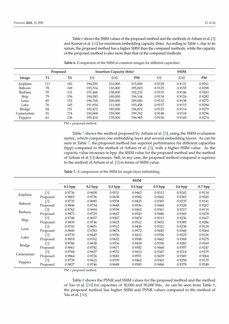
Table 6 shows the SSIM values of the proposed method and the methods of Arham

et al. [3] and Kumar et al. [16] for maximum embedding capacity (bits). According to Table

6, due to its nature, the proposed method has a higher SSIM than the compared methods,

while the capacity of the proposed method is also more than that of the compared meth-

ods.

Table 6. Comparison of the SSIM in common images for different capacities.

Proposed Insertion Capacity (bits) SSIM

Image T1 T2 [3] [24] PM [3] [24] PM

Airplane 111 182 194,250 210,000 215,000 0.9128 0.9131 0.9261

Baboon 78 149 193,314 110,000 195,003 0.9125 0.9155 0.9298

Barbara 55 131 191,466 158,000 192,232 0.9135 0.9146 0.9283

Ship 79 156 194,583 160,000 196,144 0.9134 0.9124 0.9282

Lena 85 152 196,768 200,000 209,000 0.9132 0.9138 0.9272

Lake 76 145 191,854 111,000 193,458 0.9157 0.9115 0.9284

Bridge 84 151 192,472 185,000 196,874 0.9125 0.9114 0.9279

Cameraman 91 174 194,968 159,000 199,762 0.9148 0.9118 0.9256

Peppers 61 136 195,414 178,000 196,985 0.9136 0.9145 0.9274

PM = proposed method.

Table 7 shows the method proposed by Arham et al. [3], using the SSIM evaluation

metric, which compares one embedding layer and several embedding layers. As can be

seen in Table 7, the proposed method has superior performance for different capacities

(bpp) compared to the method of Arham et al. [3], with a higher SSIM value. As the ca-

pacity value increases in bpp, the SSIM value for the proposed method and the method of

Arham et al. [3] decreases. Still, in any case, the proposed method compared is superior

to the method of Arham et al. [3] in terms of SSIM value.

Table 7. A comparison of the SSIM for single-layer embedding.

SSIM

0.1 bpp 0.2 bpp 0.3 bpp 0.4 bpp 0.5 bpp 0.6 bpp 0.7 bpp

Airplane [3] 0.9736 0.9658 0.9531 0.9462 0.9312 0.9243 0.9134

Proposed 0.9865 0.9736 0.9638 0.9582 0.9462 0.9365 0.9245

Baboon [3] 0.9735 0.9685 0.9538 0.9425 0.9365 0.9235 0.9141

Proposed 0.9846 0.9734 0.9648 0.9536 0.9468 0.9328 0.9267

Barbara [3] 0.9762 0.9694 0.9539 0.9462 0.9361 0.9217 0.9119

Figure 7. Comparing the quality values for multilayer capacities in different images: (a) Airplane;(b) Baboon; (c) Barbara; (d) Ship; (e) Lena; (f) Peppers; (g) Lake; (h) Bridge [3].

Processes 2022, 10, 858 21 of 24

Table 6 shows the SSIM values of the proposed method and the methods of Arham et al. [3]and Kumar et al. [16] for maximum embedding capacity (bits). According to Table 6, due to itsnature, the proposed method has a higher SSIM than the compared methods, while the capacityof the proposed method is also more than that of the compared methods.

Table 6. Comparison of the SSIM in common images for different capacities.

Proposed Insertion Capacity (bits) SSIM

Image T1 T2 [3] [24] PM [3] [24] PM

Airplane 111 182 194,250 210,000 215,000 0.9128 0.9131 0.9261Baboon 78 149 193,314 110,000 195,003 0.9125 0.9155 0.9298Barbara 55 131 191,466 158,000 192,232 0.9135 0.9146 0.9283

Ship 79 156 194,583 160,000 196,144 0.9134 0.9124 0.9282Lena 85 152 196,768 200,000 209,000 0.9132 0.9138 0.9272Lake 76 145 191,854 111,000 193,458 0.9157 0.9115 0.9284

Bridge 84 151 192,472 185,000 196,874 0.9125 0.9114 0.9279Cameraman 91 174 194,968 159,000 199,762 0.9148 0.9118 0.9256

Peppers 61 136 195,414 178,000 196,985 0.9136 0.9145 0.9274

PM = proposed method.

Table 7 shows the method proposed by Arham et al. [3], using the SSIM evaluationmetric, which compares one embedding layer and several embedding layers. As can beseen in Table 7, the proposed method has superior performance for different capacities(bpp) compared to the method of Arham et al. [3], with a higher SSIM value. As thecapacity value increases in bpp, the SSIM value for the proposed method and the methodof Arham et al. [3] decreases. Still, in any case, the proposed method compared is superiorto the method of Arham et al. [3] in terms of SSIM value.

Table 7. A comparison of the SSIM for single-layer embedding.

SSIM

0.1 bpp 0.2 bpp 0.3 bpp 0.4 bpp 0.5 bpp 0.6 bpp 0.7 bpp

Airplane [3] 0.9736 0.9658 0.9531 0.9462 0.9312 0.9243 0.9134Proposed 0.9865 0.9736 0.9638 0.9582 0.9462 0.9365 0.9245

Baboon[3] 0.9735 0.9685 0.9538 0.9425 0.9365 0.9235 0.9141

Proposed 0.9846 0.9734 0.9648 0.9536 0.9468 0.9328 0.9267

Barbara[3] 0.9762 0.9694 0.9539 0.9462 0.9361 0.9217 0.9119

Proposed 0.9873 0.9725 0.9647 0.9543 0.9486 0.9369 0.9278

Ship [3] 0.9748 0.9657 0.9567 0.9474 0.9313 0.9236 0.9167Proposed 0.9839 0.9746 0.9625 0.9512 0.9452 0.9385 0.9286

Lena[3] 0.9743 0.9651 0.9512 0.9436 0.9321 0.9238 0.9118

Proposed 0.9849 0.9783 0.9674 0.9572 0.9445 0.9368 0.9264

Lake[3] 0.9739 0.9645 0.9536 0.9412 0.9336 0.9225 0.9136

Proposed 0.9818 0.9762 0.9652 0.9548 0.9462 0.9368 0.9275

Bridge [3] 0.9786 0.9638 0.9536 0.9438 0.9356 0.9283 0.9169Proposed 0.9863 0.9782 0.9671 0.9582 0.9468 0.9397 0.9247

Cameraman[3] 0.9768 0.9637 0.9532 0.9413 0.9367 0.9214 0.9179

Proposed 0.9864 0.9726 0.9682 0.9551 0.9439 0.9369 0.9264

Peppers [3] 0.9739 0.9632 0.9539 0.9462 0.9363 0.9258 0.9179Proposed 0.9827 0.9746 0.9648 0.9583 0.9486 0.9378 0.9248

PM = proposed method.

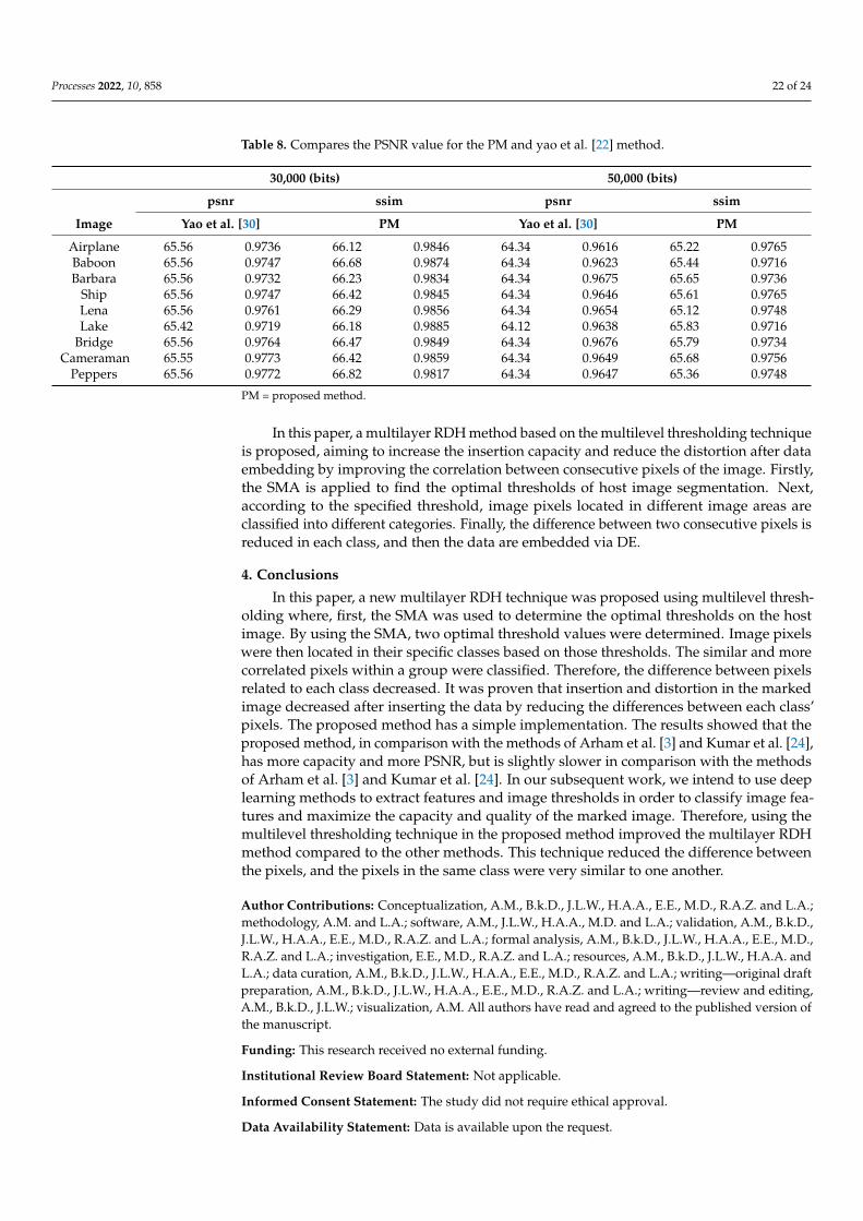
Table 8 shows the PSNR and SSIM values for the proposed method and the methodof Yao et al. [30] for capacities of 30,000 and 50,000 bits. As can be seen from Table 8,the proposed method has higher SSIM and PSNR values compared to the method ofYao et al. [30].

Processes 2022, 10, 858 22 of 24

Table 8. Compares the PSNR value for the PM and yao et al. [22] method.

30,000 (bits) 50,000 (bits)

psnr ssim psnr ssim

Image Yao et al. [30] PM Yao et al. [30] PM

Airplane 65.56 0.9736 66.12 0.9846 64.34 0.9616 65.22 0.9765Baboon 65.56 0.9747 66.68 0.9874 64.34 0.9623 65.44 0.9716Barbara 65.56 0.9732 66.23 0.9834 64.34 0.9675 65.65 0.9736

Ship 65.56 0.9747 66.42 0.9845 64.34 0.9646 65.61 0.9765Lena 65.56 0.9761 66.29 0.9856 64.34 0.9654 65.12 0.9748Lake 65.42 0.9719 66.18 0.9885 64.12 0.9638 65.83 0.9716

Bridge 65.56 0.9764 66.47 0.9849 64.34 0.9676 65.79 0.9734Cameraman 65.55 0.9773 66.42 0.9859 64.34 0.9649 65.68 0.9756

Peppers 65.56 0.9772 66.82 0.9817 64.34 0.9647 65.36 0.9748

PM = proposed method.

In this paper, a multilayer RDH method based on the multilevel thresholding techniqueis proposed, aiming to increase the insertion capacity and reduce the distortion after dataembedding by improving the correlation between consecutive pixels of the image. Firstly,the SMA is applied to find the optimal thresholds of host image segmentation. Next,according to the specified threshold, image pixels located in different image areas areclassified into different categories. Finally, the difference between two consecutive pixels isreduced in each class, and then the data are embedded via DE.

4. Conclusions

In this paper, a new multilayer RDH technique was proposed using multilevel thresh-olding where, first, the SMA was used to determine the optimal thresholds on the hostimage. By using the SMA, two optimal threshold values were determined. Image pixelswere then located in their specific classes based on those thresholds. The similar and morecorrelated pixels within a group were classified. Therefore, the difference between pixelsrelated to each class decreased. It was proven that insertion and distortion in the markedimage decreased after inserting the data by reducing the differences between each class’pixels. The proposed method has a simple implementation. The results showed that theproposed method, in comparison with the methods of Arham et al. [3] and Kumar et al. [24],has more capacity and more PSNR, but is slightly slower in comparison with the methodsof Arham et al. [3] and Kumar et al. [24]. In our subsequent work, we intend to use deeplearning methods to extract features and image thresholds in order to classify image fea-tures and maximize the capacity and quality of the marked image. Therefore, using themultilevel thresholding technique in the proposed method improved the multilayer RDHmethod compared to the other methods. This technique reduced the difference betweenthe pixels, and the pixels in the same class were very similar to one another.

Author Contributions: Conceptualization, A.M., B.k.D., J.L.W., H.A.A., E.E., M.D., R.A.Z. and L.A.;methodology, A.M. and L.A.; software, A.M., J.L.W., H.A.A., M.D. and L.A.; validation, A.M., B.k.D.,J.L.W., H.A.A., E.E., M.D., R.A.Z. and L.A.; formal analysis, A.M., B.k.D., J.L.W., H.A.A., E.E., M.D.,R.A.Z. and L.A.; investigation, E.E., M.D., R.A.Z. and L.A.; resources, A.M., B.k.D., J.L.W., H.A.A. andL.A.; data curation, A.M., B.k.D., J.L.W., H.A.A., E.E., M.D., R.A.Z. and L.A.; writing—original draftpreparation, A.M., B.k.D., J.L.W., H.A.A., E.E., M.D., R.A.Z. and L.A.; writing—review and editing,A.M., B.k.D., J.L.W.; visualization, A.M. All authors have read and agreed to the published version ofthe manuscript.

Funding: This research received no external funding.

Institutional Review Board Statement: Not applicable.

Informed Consent Statement: The study did not require ethical approval.

Data Availability Statement: Data is available upon the request.

Processes 2022, 10, 858 23 of 24

Conflicts of Interest: The authors declare no conflict of interest.

References1. Abdullah, S.M.; Manaf, A.A. Multiple Layer Reversible Images Watermarking Using Enhancement of Difference Expansion Techniques;

Springer: Berlin/Heidelberg, Germany, 2010; Volume 87, pp. 333–342.2. Zeng, X.; Li, Z.; Ping, L. Reversible data hiding scheme using reference pixel and multi-layer embedding. Int. J. Electron. Commun.

(AEÜ) 2012, 66, 532–539. [CrossRef]3. Arham, A.; Nugroho, H.A.; Adji, T.B. Multiple Layer Data Hiding Scheme Based on Difference Expansion of Quad. Signal Process.

2017, 137, 52–62. [CrossRef]4. Maniriho, P.; Ahmad, T. Information Hiding Scheme for Digital Images Using Difference Expansion and Modulus Function. J.

King Saud Univ. Comput. Inf. Sci. 2018, 31, 335–347. [CrossRef]5. Yao, H.; Qin, C.; Tang, Z.; Tian, Y. Guided filtering based color image reversible data hiding. J. Vis. Commun. Image R 2013, 43,

152–163. [CrossRef]6. Ou, B.; Li, X.; Zhao, Y. Pairwise Prediction-Error Expansion for Efficient Reversible Data Hiding. IEEE Trans. Image Process. 2013,

22, 5010–5021. [CrossRef] [PubMed]7. Li, X.; Zhang, W.; Gui, X.; Yang, B. Efficient Reversible Data Hiding Based on Multiple Histograms Modification. IEEE Trans. Inf.

Forensics Secur. 2015, 10, 2016–2027.8. Fu, D.; Jing, Z.J.; Zhao, S.G.; Fan, J. Reversible data hiding based on prediction-error histogram shifting and EMD mechanis. Int. J.

Electron. Commun. 2014, 68, 933–943. [CrossRef]9. Ou, B.; Li, X.; Wang, J.; Peng, F. High-fidelity reversible data hiding based on geodesic path and pairwise prediction-error

expansion. Neurocomputing 2016, 68, 933–943. [CrossRef]10. Wang, J.; Ni, J.; Zhang, X.; Shi, Y.Q. Rate and Distortion Optimization for Reversible Data Hiding Using Multiple Histogram

Shifting. IEEE Trans. Cybern. 2016, 47, 315–326. [CrossRef]11. Xiao, M.; Li, X.; Wang, Y.; Zhao, Y.; Ni, R. Reversible data hiding based on pairwise embedding and optimal expansion path.

Signal Process. 2019, 19, 30017–30019. [CrossRef]12. Zhou, H.; Chen, K.; Zhang, W.; Yu, N. Comments on Steganography Using Reversible Texture Synthesis. IEEE Trans. Image

Process. 2017, 26, 1623–1625. [CrossRef] [PubMed]13. Shehab, M.; Abualigah, L.; Shambour, Q.; Abu-Hashem, M.A.; Shambour, M.K.Y.; Alsalibi, A.I.; Gandomi, A.H. Machine learning

in medical applications: A review of state-of-the-art methods. Comput. Biol. Med. 2022, 145, 105458. [CrossRef] [PubMed]14. Zhu, X.; Zhou, M. Multiobjective Optimized Cloudlet Deployment and Task Offloading for Mobile-Edge Computing. IEEE

Internet Things J. 2021, 8, 15582–15595. [CrossRef]15. Zhu, Q.-H.; Tang, H.; Huang, J.-J.; Hou, Y. Task Scheduling for Multi-Cloud Computing Subject to Security and Reliability

Constraints. IEEE/CAA J. Autom. Sin. 2021, 8, 848–865. [CrossRef]16. Ezugwu, A.E.; Ikotun, A.M.; Oyelade, O.O.; Abualigah, L.; Agushaka, J.O.; Eke, C.I.; Akinyelu, A.A. A comprehensive survey of

clustering algorithms: State-of-the-art machine learning applications, taxonomy, challenges, and future research prospects. Eng.Appl. Artif. Intell. 2022, 110, 104743. [CrossRef]

17. Otair, M.; Abualigah, L.; Qawaqzeh, M.K. Improved near-lossless technique using the Huffman coding for enhancing the qualityof image compression. Multimed. Tools Appl. 2022, 1–21. [CrossRef]

18. Tang, J.; Liu, G.; Pan, Q. A Review on Representative Swarm Intelligence Algorithms for Solving Optimization Problems:Applications and Trends. IEEE/CAA J. Autom. Sin. 2021, 8, 1627–1643. [CrossRef]

19. Abualigah, L.; Abd Elaziz, M.; Sumari, P.; Geem, Z.W.; Gandomi, A.H. Reptile Search Algorithm (RSA): A nature-inspiredmeta-heuristic optimizer. Expert Syst. Appl. 2022, 191, 116158. [CrossRef]

20. He, W.; Cai, J.; Xiong, G.; Zhou, K. Improved reversible data hiding using pixel-based pixel value grouping. Optik 2017, 157,68–78. [CrossRef]

21. He, W.; Xiong, G.; Zhou, K.; Cai, J. Reversible data hiding based on multilevel histogram modification and pixel value grouping.J. Vis. Commun. Image Represent. 2016, 40, 459–469. [CrossRef]

22. Li, X.; Li, J.; Li, B.; Yang, B. High-fidelity reversible data hiding scheme based on pixel-value-ordering and prediction-errorexpansion. Signal Process. 2013, 93, 198–205. [CrossRef]

23. Kumar, R.; Jung, K.H. Robust reversible data hiding scheme based on two-layer embedding strategy. Inf. Sci. 2020, 512, 96–107.[CrossRef]

24. Kumar, R.; Kim, D.S.; Jung, K.H. Enhanced AMBTC based data hiding method using hamming distance and pixel valuedifferencing. J. Inf. Secur. Appl. 2019, 47, 94–103. [CrossRef]

25. Kim, P.H.; Ryu, K.W.; Jun, K.H. Reversible data hiding scheme based on pixel-value differencing in dual images. Int. J. Distrib.Sens. Netw. 2020, 16, 1550147720911006. [CrossRef]

26. Hussain, M.; Riaz, Q.; Saleem, S.; Ghafoor, A.; Jung, K.H. Enhanced adaptive data hiding method using LSB and pixel valuedifferencing. Multimed. Tools Appl. 2021, 80, 20381–20401. [CrossRef]

27. Yu, C.; Zhang, X.; Zhang, X.; Li, G.; Tang, Z. Reversible Data Hiding with Hierarchical Embedding for Encrypted Images. IEEETrans. Circuits Syst. Video Technol. 2021, 32, 451–466. [CrossRef]

Processes 2022, 10, 858 24 of 24

28. Tang, Z.; Nie, H.; Pun, C.M.; Yao, H.; Yu, C.; Zhang, X. Color Image Reversible Data Hiding with Double-Layer Embedding. IEEEAccess 2020, 8, 6915–6926. [CrossRef]

29. Yao, H.; Mao, F.; Tang, Z.; Qin, C. High-fidelity dual-image reversible data hiding via prediction-error shift. Signal Process. 2020,170, 107447. [CrossRef]

30. Salehnia, T.; Izadi, S.; Ahmadi, M. Multilevel image thresholding using GOA, WOA and MFO for image segmentation. InProceedings of the 8th International Conference on New Strategies in Engineering, Information Science and Technology in theNext Century, Dubai, United Arab Emirates (UAE), 2021; Available online: https://civilica.com/doc/1196572/ (accessed on 16March 2022).

31. Raziani, S.; Salehnia, T.; Ahmadi, M. Selecting of the best features for the knn classification method by Harris Hawk algorithm. InProceedings of the 8th International Conference on New Strategies in Engineering, Information Science and Technology in theNext Century, Dubai, United Arab Emirates (UAE), 2021; Available online: https://civilica.com/doc/1196573/ (accessed on 16March 2022).

32. Salehnia, T.; Fath, A. Fault tolerance in LWT-SVD based image watermarking systems using three module redundancy technique.Expert Syst. Appl. 2021, 179, 115058. [CrossRef]

33. El Aziz, M.A.; Ewees, A.A.; Hassanien, A.E. Whale Optimization Algorithm and Moth-Flame Optimization for MultilevelThresholding Image Segmentation. Expert Syst. Appl. 2017, 83, 242–256. [CrossRef]

34. Akay, B. A study on particle swarm optimization and artificial bee colony algorithms for multilevel thresholding. Appl. SoftComput. 2013, 13, 3066–3091. [CrossRef]

35. Li, S.; Chen, H.; Wang, M.; Heidari, A.A.; Mirjalili, S. Slime mould algorithm: A new method for stochastic optimization. FutureGener. Comput. Syst. 2020, 111, 300–323. [CrossRef]

36. Liu, H.; Zhou, M.; Guo, X.; Zhang, Z.; Ning, B.; Tang, T. Timetable Optimization for Regenerative Energy Utilization in SubwaySystems. IEEE Trans. Intell. Transp. Syst. 2019, 20, 3247–3257. [CrossRef]

37. Abualigah, L.; Yousri, D.; Abd Elaziz, M.; Ewees, A.A.; Al-Qaness, M.A.; Gandomi, A.H. Aquila optimizer: A novel meta-heuristicoptimization algorithm. Comput. Ind. Eng. 2021, 157, 107250. [CrossRef]

38. Agushaka, J.O.; Ezugwu, A.E.; Abualigah, L. Dwarf mongoose optimization algorithm. Comput. Methods Appl. Mech. Eng. 2022,391, 114570. [CrossRef]