A New Osteophyte Segmentation Algorithm Using the Partial Shape Model and Its Applications to Rabbit...

2212 IEEE TRANSACTIONS ON BIOMEDICAL ENGINEERING, VOL. 58, NO. 8, AUGUST 2011

A New Osteophyte Segmentation Algorithm Usingthe Partial Shape Model and Its Applications to

Rabbit Femur Anterior Cruciate LigamentTransection via Micro-CT Imaging

P. K. Saha*, Member, IEEE, G. Liang, J. M. Elkins, A. Coimbra, L. T. Duong, D. S. Williams,and M. Sonka, Fellow, IEEE

Abstract—Osteophyte is an additional bony growth on a nor-mal bone surface limiting or stopping motion at a deterioratingjoint. Detection and quantification of osteophytes from computedtomography (CT) images is helpful in assessing disease status aswell as treatment and surgery planning. However, it is difficult todistinguish between osteophytes and healthy bones using simplethresholding or edge/texture features due to the similarity of theirmaterial composition. In this paper, we present a new method pri-marily based on the active shape model (ASM) to solve this prob-lem and evaluate its application to the anterior cruciate ligamenttransaction (ACLT) rabbit femur model via micro-CT imaging.The common idea behind most ASM-based segmentation meth-ods is to first build a parametric shape model from a trainingdataset and then apply the model to find a shape instance in atarget image. A common challenge with such approaches is thata diseased bone shape is significantly altered at regions with os-teophyte deposition misguiding an ASM method and eventuallyleading to suboptimum segmentations. This difficulty is overcomeusing a new partial-ASM method that uses bone shape over healthyregions and extrapolates it over the diseased region according tothe underlying shape model. Finally, osteophytes are segmented bysubtracting partial-ASM-derived shape from the overall diseasedshape. Also, a new semiautomatic method is presented in this paperfor efficiently building a 3-D shape model for an anatomic regionusing manual reference of a few anatomically defined fiducial land-marks that are highly reproducible on individuals. Accuracy of themethod has been examined on simulated phantoms while repro-ducibility and sensitivity have been evaluated on micro-CT imagesof 2-, 4- and 8-week post-ACLT and sham-treated rabbit femurs.

Manuscript received October 22, 2010; revised January 23, 2011; acceptedFebruary 15, 2011. Date of publication March 17, 2011; date of current ver-sion July 20, 2011. This work was supported in part by the Merck/UIowa Os-teophyte Segmentation Study under Agreement X2924461. Asterisk indicatescorresponding author.

*P. K. Saha is with the Department of Electrical and Computer Engineeringand the Department of Radiology, the University of Iowa, Iowa City, IA 52242USA (e-mail: [email protected]).

G. Liang and M. Sonka are with the Department of Electrical and Com-puter Engineering, the University of Iowa, Iowa City, IA 52242 USA (e-mail:[email protected]; [email protected]).

J. M. Elkins is with the Department of Orthopaedic Surgery, the Universityof Iowa, Iowa City, IA 52242 USA (e-mail: [email protected]).

A. Coimbra and D. S. Williams are with the Imaging, Merck Research Labo-ratories, West Point, PA 19486 USA (e-mail: [email protected];[email protected]).

L. T. Duong is with the Bone Biology, Merck Research Laboratories, WestPoint, PA 19486 USA (e-mail: [email protected]).

Color versions of one or more of the figures in this paper are available onlineat http://ieeexplore.ieee.org.

Digital Object Identifier 10.1109/TBME.2011.2129519

Experimental results have shown that the method is highly ac-curate (R2 = 0.99), reproducible (ICC = 0.97), and sensitive indetecting disease progression (p values: 0.065, 0.001, and <0.001for 2 weeks versus 4 weeks, 4 weeks versus 8 weeks, and 2 weeksversus 8 weeks, respectively).

Index Terms—Active shape model (ASM), anterior cruciate lig-ament transection (ACLT), micro-computed tomography (micro-CT) imaging, osteophyte, rabbit femur, segmentation.

I. INTRODUCTION

MUSCULOSKELETAL disorders are associated with theformation of new bones at two main sites—the joint

margin (osteophytosis) and ligament and tendon insertions (en-thesophyte formation) [1], [2]. An osteophyte is an additionalbony growth on a normal bone surface limiting or stopping mo-tion at a deteriorating joint and often pressurizing nearby nervescausing pain and sometimes debilitating medical conditions.Osteophytes are strongly associated with osteoarthritis (OA),probably developing in response to abnormal stress on the jointmargin [3]. There is also evidence in literature that marginalosteophytes may develop as an age-related phenomenon not re-lated to any joint disease [4]. OA is a progressive joint diseasecharacterized by cartilage degradation and bone remodeling.OA affects nearly 27 million people in the U.S. and problemswith ambulation secondary to OA may account for ≥25% ofvisits to primary care physicians, so the burden to society isquite high [5]. It is estimated that 80% of the population willhave radiographic evidence of OA by the age of 65, althoughonly 60% of those will show symptoms [5]. Several researchreports exist in the literature studying the size and the patternof osteophyte distributions in patients with symptoms of OA indifferent joints [6]–[9].

Besides pain and other OA related symptoms, osteophytesmay also lead to development of other diseases including dys-phagia [10] and pneumonia [11]. However, osteophytes may notalways lead to clinical symptoms and some are formed as a partof the normal aging process [4]. Also, osteophytes may not re-quire treatment unless they are causing pain or damaging othertissues. Recently, there has been research interest in studyingthe role of retained osteophytes in causing pain and other symp-toms in patients with total knee or hip arthroplasty [12], [13].An effective tool to detect and derive a quantitative measure ofosteophyte morphology in patients will be helpful in clinical and

0018-9294/$26.00 © 2011 IEEE

SAHA et al.: NEW OSTEOPHYTE SEGMENTATION ALGORITHM USING THE PARTIAL SHAPE MODEL AND ITS APPLICATIONS 2213

research studies and in understanding the cause and etiology ofrelated disease progression. Such a tool may prove useful for di-agnostic purposes and for planning and monitoring surgical andtherapeutic interventions. Radiographs provide an insensitiveand inaccurate way of detecting the shape and position of os-teophytes [14], [15]. Recently, MRI and computed tomography(CT) imaging modalities, which provide 3-D information, havebeen adopted for osteophyte detection and quantification [6],[16]–[18]. However, these methods rely on visual detection andscoring of osteophytes in 3-D images. In this paper, we presenta new method for osteophyte segmentation and quantification.We evaluate its performance using simulated phantoms as wellas micro-CT images of distal femurs from an anterior cruciateligament transection (ACLT) rabbit model [18], [19].

Image segmentation is a process of identifying and delineat-ing the spatial extent of a target object in an image. There areseveral established approaches for image segmentation, and ex-tended surveys on medical image segmentation methods existin the literature [20]. Despite a large number of segmentationapproaches available in the literature, it has remained an activeresearch area due to unique requirements by individual segmen-tation tasks. In this paper, we design a method for segmentingosteophytes in micro-CT images which may also be useful tosegment and quantify osteophytes in patients via CT imaging.Development of such methods is important as it is difficult todistinguish between osteophytes and healthy bones using sim-ple thresholding or edge/texture features due to the similarity oftheir material composition. We, therefore, present a new methodprimarily based on the active shape model (ASM) to solve thisproblem and evaluate its application to the ACLT rabbit femurmodel via micro-CT imaging. The premise of our method isto, first, determine the healthy bone in the image scan data andthen subtract it leading to segmentation of osteophytes. Thistwo-step approach facilitates reducing segmentation errors in-duced by wide variations in shape, smoothness, and size ofosteophytes.

The common idea behind most ASM-based segmentationmethods [21] is to first build a parametric shape model froma training dataset and then apply the model to locate a shapeinstance in a given test image. However, such an approach facesan immediate self-imposing challenge due to the fact that boneshape/geometry is maximally distorted at regions affected byosteophyte deposition. Therefore, a straightforward applicationof a prior-shape model to determine the target shape in a testimage is bound to be influenced by the geometry of the osteo-phyte itself. A possible solution to this problem is to use theshape information from healthy bone surface regions and usethat information to extrapolate the original surface at regionsaffected by osteophytes. This observation has inspired us to for-mulate a new approach, called the partial ASM (pASM) thatuses bone geometry over regions with higher compliance to theprior shape model and uses the so-computed shape parametersto extrapolate bone shape over regions with imperfect matchpossibly due to osteophyte presence. Another important contri-bution of this paper is to design a generic approach to build anASM for a 3-D object using interactive inputs for a few fiduciallandmarks (LMs) that are reproducibly locatable in a training

Fig. 1. (a) and (b) 3-D renditions of rabbit femur bones with and withoutosteophytes. (c) 2-D display of osteophytes in a micro-CT image; no visibleintensity difference exists between osteophytes and healthy bones. (d) Exampleof osteophyte segmentation by a conventional ASM approach.

dataset. Experimental results evaluating the method’s accuracy,reproducibility, and sensitivity based on simulated phantomsand micro-CT images of ACLT rabbit femurs are presented.Theory and algorithms for a new method to build an ASM forany 3-D anatomic body region along with the pASM are pre-sented in Section II. Methods and the experimental setup for thespecific application of segmenting osteophytes in ACLT rabbitfemur via micro-CT imaging are described in Section III. Fi-nally, all experimental results are discussed and conclusions aredrawn in Section IV.

II. THEORY AND ALGORITHMS

An osteophyte or bone spur [see Fig. 1(a)] is an additionalbony growth on a normal bone surface [see Fig. 1(b)] whichis often difficult to separate from the healthy bone using sim-ple thresholding in CT/micro-CT imaging as demonstrated inFig. 1(c). As illustrated in Fig. 1(d), a straightforward applica-tion of a shape-model-based approach, e.g., the ASM, fails tosegment the healthy bone in the presence of osteophytes dueto the influence of diseased regions. As mentioned earlier, thisdifficulty is overcome by using a new approach of the pASMintroduced in this paper. Theoretical and methodological devel-opments related to 3-D shape model generation are described inSection II-A while those related to the pASM are presented inSection II-B.

A. New Approach to 3-D Active Shape Modeling

Major challenges in developing a shape model for a givenanatomic structure lie in defining the anatomic shape as an or-dered set of LMs on each individual shape instance in a trainingdataset. Although the task is less challenging in two dimensions(2-D), it is not the case in 3-D. Several research works have


Fig. 2. Salient (solid dots) and derived (hollow dots) LMs on a 2-D contourof a hand.

been reported in the literature on 3-D LM generation towarddeveloping a shape model [22]–[31]. Kelemen et al. [22] solvedthe 3-D point correspondence problem through a shape pa-rameterization technique by using spherical harmonics. Davieset al. [29] introduced a new approach that poses the LM cor-respondence task as an optimization problem on the qualityof the statistical model that minimizes the description lengthof the resulting model. This approach has further been stud-ied and improved by Thodberg [30] and Heimann et al. [31].Registration-based approaches have been adopted by severalresearch groups [23]–[28] to develop the correspondence of3-D LMs within a set of training shapes. Brett and Taylor [23]developed a framework for automatic 3-D LM generation viaa binary tree of registered and merged pairs of shapes, eachrepresented by a set of polygonal contours which was furthermodified in [24]. Wang et al. [25] used a surface-registrationmethod based on a metric matching surface-to-surface distance,surface normal, and curvature to establish the correspondenceof 3-D LMs. Frangi et al. [26]–[28] have used a volumetricfree-form elastic registration technique based on the maximiza-tion of normalized mutual information to build the 3-D LMcorrespondence within the set of training shapes.

Here, we develop a new method for defining the shape modelof a given 3-D anatomic surface inspired by the approach weintuitively follow in 2-D. For example, while defining the shapemodel of a hand, we indicate a few salient points (solid dots inFig. 2) and then automatically include a predefined number ofequispaced additional points (hollow dots in Fig. 2) in betweenevery two successive salient points. On a 3-D anatomic surface,often, several curves and LM points may anatomically be de-fined and manually detected with high reproducibility; we referto these LMs as fiducial LMs. The idea is to interactively indicatesuch curves and LM points on a given shape using a graphicalinterface and use these curves and LM points as reference todivide the entire 3-D surface into subsurface regions. Using thereference of interactive fiducial LMs, additional LMs are auto-matically located on each subregion according to a predefineddistribution; we refer to such LMs as secondary LMs. We arguethat such an approach is more reproducible and efficient lead-ing toward an optimal tradeoff between automatic and manuallandmarking. The presented approach of 3-D LM generation

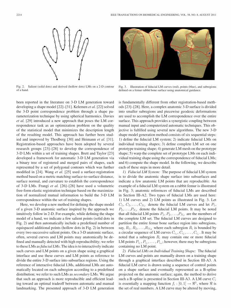
Fig. 3. Illustration of fiducial LM curves (red), points (blue), and subregionsdefined on a femur rabbit bone surface using anatomical guidance.

is fundamentally different from other registration-based meth-ods [23]–[28]. Here, a complex anatomic 3-D surface is dividedinto smaller subregions and piecewise geodesic deformationsare used to accomplish the LM correspondence over the entiresurface. This approach provides a synergistic coupling betweenmanual input and computerized automatic techniques. This ob-jective is fulfilled using several new algorithms. The new 3-Dshape model generation method consists of six sequential steps:1) define the fiducial LM system; 2) indicate fiducial LMs onindividual training shapes; 3) define complete LM set on oneprototype training shape; 4) generate LM mesh on the prototypeshape; 5) warp the complete set of prototype LMs on each indi-vidual training shape using the correspondence of fiducial LMs;and 6) compute the shape model. In the following, we describeeach of these steps in more detail.

1) Fiducial LM System: The purpose of fiducial LM systemis to divide the anatomic shape surface into subsurfaces andindicate a few anatomic LM points that are reproducible. Anexample of a fiducial LM system on a rabbit femur is illustratedin Fig. 3; anatomic references of fiducial LMs are describedin Section III-A2. Two types of fiducial LMs are used here:1) LM curves and 2) LM points as illustrated in Fig. 3. LetC1 , C2 , . . . , CNC

denote the fiducial LM curves and let P1 ,P2 , . . . ,PNP

denote the fiducial LM points. It may be notedthat all fiducial LM points P1 , P2 , . . . ,PNP

are the members ofthe complete LM set. The fiducial LM curves are designed topartition the entire femur bone surface region into subregions,say, R1 , R2 , . . . ,RNR

where each subregion Ri is bounded bya circular sequence of LM curves Ci1 , Ci2 , . . . , Cin

. It may benoted that a subregion Ri may contain one or more fiducialLM points Pi1 , Pi2 , . . . , Pim

; however, there may be subregionscontaining no LM point.

2) Fiducial LMs on Individual Training Shape: The fiducialLM curves and points are manually drawn on a training shapethrough a graphical interface described in Section III-A3. Afiducial LM curve is drawn using a sequence of control pointson a shape surface and eventually represented as a B-splineprojected on the anatomic surface; again, the method to derivesuch a B-spline is presented in Section III-A3. A LM curve Ci

is essentially a mapping function fi : [0, 1] → �3 , where � isthe set of real numbers. A LM curve may be altered by moving,


Fig. 4. (a) 3-D rendition of a binarized rabbit femur bone data used as a training shape. (b) Surface-mesh representation of (a). A zoom-in representation of thesurface mesh is presented on the left to illustrate the mesh structure and triangle density. (c) Graphical illustration of the mesh augmentation process; see the textfor details. (d) Manifold distance transform from LM points; the color bar is given on the right. (e) Color-coded display of nearest geodesic neighbor; here eachLM is represented by a unique color.

deleting, or adding its control points. Finally, a fiducial LM pointPi is a point on the anatomic surface of a given training shape.

3) Complete LM Set on a Prototype Training Shape: One ofthe training data is used as a prototype shape and the completeset of LMs, denoted by Ω, is defined on the prototype shape withreference to its fiducial LMs. As discussed earlier, the completeLM set should contain both fiducial as well as secondary LMs.Following the shape model theory [21], Ω must be an orderedset of a predefined number of LM points. To comply with thisrequirement, a set of a predefined number of equispaced LMsare automatically identified on each LM curve. Now onward,a fiducial LM point or an automatically identified LM pointon a fiducial LM curve will be referred to as a primary LM.Furthermore, for each anatomic subregion Ri on the prototypeshape, an extended list of secondary LMs is interactively spec-ified through a graphical interface at an approximate uniformdistribution. Let Π denote the set of all primary LMs and let Θdenote the set of all secondary LMs; thus, the complete LM setΩ = Π ∪ Θ. We will use Πi and Θi to denote the set of primaryand secondary LMs on the subregion Ri . In general, we will usep and s to refer to a primary and a secondary LM, respectively,and l to refer to any LM from Ω.

4) LM Mesh Generation: The LM mesh on a given trainingshape is generated from its binary representation using the fol-lowing steps. First, a surface mesh representation of a binaryobject [see Fig. 4(a)] is computed using the marching cube al-gorithm [32]. This surface mesh is highly dense [see Fig. 4(b)]yielding around 15–20 thousand triangles and consists of thefinest elements in our computational framework determining theintrinsic precision of the method. The LM mesh that is much

coarser in resolution is generated using the following steps:1) augmentation of surface-mesh ensuring that each LM in Ωis a vertex of the surface mesh; 2) computation of manifolddistance transform; and 3) manifold Delaunay triangulation andLM mesh generation.

Augmentation of surface mesh: The primary objective of thisstep is to ensure that each LM is a vertex of the final surfacemesh. A mesh is represented by a pair Υ = (V,E), where Vis the set of all vertices and E is the set of all edges in Υ. Themarching cube algorithm ensures that the vertices and the edgesin Υ partition the entire surface into triangular elements whilemaintaining the topology of the surface. However, a primary ora secondary LM is not necessarily a vertex of the surface meshwhich is computed independently. In case an LM is not a vertexof the surface mesh, it may either be located inside a surface-mesh triangle or on its edge. When an LM l falls inside a triangle�abc, where a, b, and c are the surface-mesh vertices, the trian-gle �abc is replaced by three smaller triangles, namely, �abl,�lbc, and �alc and therefore the original mesh Υ = (V,E) isaugmented to Υaug = (V ∪ {l}, E ∪ {al, bl, cl}). On the otherhand, if l falls on an edge ab, the triangle �abc is replacedby two triangles �alc and �blc and the mesh is modifiedto Υaug = (V ∪ {l}, (E − {ab}) ∪ {al, bl, cl}). These meshaugmentation steps are illustrated in Fig. 4(c). In the sub-sequent discussion, a surface mesh Υ will refer to the aug-mented surface mesh with every LM being a vertex of themesh.

Computation of manifold distance transform: The intuitiveidea behind this step is to generate a geodesic Voronoi neigh-borhood diagram of the LMs embedded on a surface mesh.


Computation of planar Voronoi neighborhood diagram [33] isaccomplished using regular Euclidean distance metric. On theother hand, a manifold distance metric is necessary to computemanifold Voronoi neighborhood diagram which is described inthe following.

A path π on a surface mesh Υ = (V,E) between two verticesv1 , v2 ∈ V is a sequence of edges 〈e1 , e2 , . . . , en 〉 | ∀i, ei ∈ Ethat satisfies the following three conditions.

1) v1 is a vertex of e1 .2) v2 is a vertex of en .3) ei and ei+1 share a common vertex.The length of a path π = 〈e1 , e2 , . . . , en 〉, denoted byL(π), is

defined as L(π) =∑n

i=1 |ei |, where |ei | denotes the Euclideanlength of the edge ei . There are infinitely many paths on a surfacemesh between any two vertices; let P(v1 , v2 ,Υ) denote the setof all paths on a surface mesh Υ between two vertices v1 andv2 . Finally, the manifold distance D(v1 , v2 ,Υ) between v1 andv2 on Υ is defined as follows:

D(v1 , v2 ,Υ) = minπ∈P(v1 ,v2 ,Υ)

L(π).

In order to compute the manifold Voronoi neighborhood dia-gram, we need to determine manifold distance transform fromLMs along with the information about the nearest LM. This ob-jective is fulfilled using the following algorithm, where NΥ(v)denotes the neighborhood of v in the mesh Υ that is defined asthe set of all vertices in Υ sharing an edge with v:

begin: compute_manifold_distance_transforminput: surface-mesh Υ = (V,E)

set Ω of all LMsoutput: manifold distance transform map MDT : V → �

nearest LM map NLM : V → Ωinitialize an empty queue Q

for all v ∈ VMDT(v) = MaxValueNLM(v) = −1

for all l ∈ ΩMDT(l) = 0NLM(l) = lpush l in Q

while Q is not emptypop v from Qfor all v′ ∈ NΥ(v)

if MDT(v′) > MDT(v) + |vv′|MDT(v′) = MDT(v) + |vv′|NLM(v′) = NLM(v)push v′ in Q

end compute_manifold_distance_transformA result of the aforementioned algorithm is presented in

Fig. 4(d) and (e) illustrating both manifold distance transformand manifold Voronoi neighborhood, which is essentially de-picting the nearest LM map.

LM mesh generation: LM mesh is generated using the resultsof the manifold distance transform described in the previoussection. Specifically, the LM mesh is created as the manifoldDelaunay triangulation of the surface mesh derived using themanifold distance transform and the nearest LM map as follows:

begin: generate_LM_meshinput: surface-mesh Υ = (V,E)

set of all LMs Ωnearest LM map NLM : V → Ω

output: LM-mesh Ψ = (Ω, EΩ)initialize an LM-mesh Ψ = (Ω, EΩ = empty set)

all v ∈ Vl1 = NLM(v)

for all v′ ∈ NΥ(v)

l2 = NLM(v′)

if l1 �= l2 and l1 l2 /∈ EΩEΩ = EΩ ∪ l1 l2

end generate_LM_meshTo illustrate how the method works, the LM mesh, or, equiv-

alently, the manifold Delaunay triangulation is simultaneouslyshown in Fig. 4(e) with color-coded manifold Voronoi neigh-borhoods of LMs.

Here, an interesting question may transpire as whether theaforementioned LM generation method creates unnecessaryedges in a mesh destabilizing its topology. Topological stabil-ity may be examined at each individual vertex in the LM meshΨ = (Ω, EΩ) as follows. A vertex v ∈ Ω is a stable vertex if itsneighboring vertices v0 , v1 , . . . , vn−1 ∈ Ω form a unique cycli-cal order of the edges v0v1 , v1v2 , . . . , vn−2vn−1 , vn−1v0 ∈ EΩcreating a simple closed loop and vivj /∈ EΩ for all j �= i ± 1mod n. As examined using a computerized algorithm, the afore-mentioned algorithm has always generated a stable surface meshfor the datasets used in our experiment. It may be noted that,even if the method fails to generate a topologically stable meshin an adverse situation, the instance may automatically be de-tected and unnecessary edges may be deleted.

Deformation of reference LMs onto another bone surface:The basic idea of this step is to map secondary LMs of a refer-ence surface onto a target surface using the correspondence oftheir primary LMs. This task is accomplished using piecewisedeformation of each subregion of the reference surface onto thecorresponding subregion of the target surface, where the corre-spondence of two subregions is defined by their primary LMs.Let R denote a subregion on the reference surface containing theprimary LMs p1 , p2 , . . . , pn and secondary LMs s1 , s2 , . . . , sm

and let R′ denote the matching subregion on the target surfacecontaining primary LMs p′1 , p

′2 , . . . , p

′n . Note that, at this stage

of computation, no information is available about secondaryLMs on the target surface. The problem here is to deform thesecondary LMs s1 , s2 , . . . , sm onto the target subregion R′ suchthat 1) the correspondence of primary LMs in two surfaces ispreserved, i.e., pi is mapped onto p′i for all i = 1, 2, . . . , n and2) the geometry of the LM mesh in R is minimally changedafter mapping secondary LMs of R onto R′. A method similarto a physical process of spring-mesh deformation is adoptedhere as follows. Let ER ⊂ EΩ denote the set of the edges suchthat one endpoint of the edge is a secondary LM inside R andthe other end is any LM of R; thus, ER along with the LMs ofR describe the LM mesh over the subregion R. Note that ER

excludes all edges between two primary LMs on R. A springmesh with uniform spring constant is constructed by replacingeach edge of ER with a spring of length equal to that of the edge


Fig. 5. Results of reference LM mesh deformation onto a target surface. (a) Initial superimposition of reference mesh (red: LM, green: edge) with the targetsurface. Results on one subregion: (b) affine alignment of primary LMs using Procrustes analysis and (c) topology preserving elastic deformation of reference LMmesh onto the target surface. Reference: red (primary LM), blue (secondary LM), and green (spring-edge). Target: yellow (primary LM).

itself [green edges in Fig. 5(b)]. A manifold spring deformationprocess is adopted that starts with the best possible alignmentbetween pis (red dots) and p′is (yellow dots). Subsequently, eachpi gradually moved toward p′i using an external force and thesecondary LMs are allowed to freely move along the surfaceof R′ governed by the spring force system while preserving themesh topology. Each primary LM moves in straight line join-ing its initial and final positions. However, to ensure that thefinal destination of a secondary LM lies on the geodesic of R′,its movements is always constricted along the geodesic of thetarget surface. To complete the description of the process, theforce system and the mesh topology preserving conditions aredefined in the following paragraph.

The LM mesh deformation process is defined as an itera-tive process and the duration of each iteration is a predefinedconstant ∇t. At any time/iteration t during the deformation pro-cess, two different types of forces are used—one for primaryLMs and the other for secondary LMs. As mentioned before,the mesh deformation process is initialized by aligning primaryLMs p1 , p2 , . . . , pn of R with the LMs p′1 , p

′2 , . . . , p

′n of R′, re-

spectively, using the affine transform τ computed by Procrustesanalysis [34] [see Fig. 5(b)]. Thus, pi(t = 0) = τ (pi) denotesinitial position of a primary LM pi in the process of deformingthe reference LM mesh of R onto the target subregion R′. Sim-ilarly, si(t = 0) = τ (si) denotes initial position of a secondaryLM si during the deformation process. At any time t during thedeformation process, a force Fp(pi, t) on a primary LM pi(t) isdesigned to gradually move pi toward p′i and is defined as a con-stant force along the vector p′i − pi(t). The oscillation aroundthe target point p′i is avoided by forcing pi(t) to move to p′i at theend of iteration when they become sufficiently close; it avoidsoscillation by stopping over movements. The force Fs(si, t) ona secondary LM si is designed to serve two purposes: 1) toenforce the deformation along the geodesic of the target sur-face R′ and 2) to simulate a spring mesh deformation. The first

component of the force is much larger compared to the secondcomponent. During the early part of the deformation process,the first component of the force serves the purpose of projectingsi onto the target surface mesh Υ′ = (V ′, E′). At any time tduring the deformation process, the magnitude of this force onsi is proportional to the distance of si(t) from Υ′ and is di-rected toward the closest surface-mesh vertex v ∈ V ′; let us useFDT (x,Υ′) to denote the force on any point x ∈ �3 that pullsx toward the surface Υ′. At any time t during the deformationprocess, the spring force Fsp(si, sj , t) on an LM si due to theedge sisj is governed by the following equation:

Fsp(si, sj , t) = K × (lorig (si, sj ) − |si(t) − sj (t)|)lorig (si, sj )

× (si(t) − sj (t))|si(t) − sj (t)|

where K is the spring constant and the function lorig (si, sj )gives the original length of the edge connecting the two LMssi and sj after the affine transformation τ , i.e., lorig (si, sj ) =|τ (si) − τ (sj )|. Finally, the total force Fs(si, t) on a secondaryLM si at time t is defined as follows:

Fs(si, t) = FDT (si(t),Υ′) +∑

l∈NΨ (si )

Fspring(si, l, t)

where NΨ(si) denotes the neighborhood of si in the LM mesh.Two additional constraints are imposed on the deformation ofsecondary LMs to preserve a mesh topology and to avoid meshfolding on the target surface as described in the following. Letu denote the new position of an LM si after applying the forceFs(si, t), as defined earlier, over a duration of ∇t. This moveis allowed, i.e., si(t + ∇t) is updated to u, if it preserves themesh topology and creates no folding through the narrow spacebetween the target surface and the deforming LM mesh itself(see Fig. 6). This phenomenon of folding, mostly associated with


Fig. 6. Schematic illustration of LM mesh folding through the narrow spacebetween the target surface and deforming LM mesh. Mesh configuration before(a) and after (b) folding. The triangle �abc flips on the other side of the edge bcand slides through the narrow space between the mesh surface (shown by blacklines) and the underlying target surface. Different shadings are used to denotelayerwise depths with black lines being front most. Such situation creates atopological aberration of the surface mesh by “folding”.

a geodesic mesh deformation, seems to be a new observationand may easily be confused with mesh topology violation. Sucha phenomenon occurs when the springs attached to a specificvertex [e.g., vertex a in Fig. 6(a)] gets highly compressed. Dueto finite step size of iterations during the deformation process,under high compression, the vertex a may flip on the other sideof the most convenient edge [the edge bc, Fig. 6(a)] and glidesthrough the narrow space between the triangle �ebc and thebone surface beneath the mesh [see Fig. 6(b)]. Essentially, thevertex a creates a folding at the edge bc to produce some extrageodesic space releasing the high compression exerted on itself.A solution to this problem is to never allow an LM to come closeto another LM or an edge of the LM mesh or an LM triangle.On the other hand, a mesh topology is altered under one of thefollowing three conditions: 1) an LM coincides with anotherLM; 2) an LM transects an edge of the LM mesh; and 3) anLM transects through a mesh triangle. The final result of an LMmesh generated using the topology preserving the elastic meshdeformation algorithm is presented in Fig. 5(c).

B. Partial Active Shape Model

A shape of an anatomic structure is mathematically repre-sented using the mean shape as well as shape variations observedin the set of training shapes leading to an ASM [21]. Followingthe outline by Cootes and Taylor [21], the mean as well as vari-ations in an anatomic shape is computed using the Procrustesmethod [35] and principal component analysis (PCA). Specifi-cally, in 3-D, the mean shape is represented as a 3N-D vector μand the shape model is expressed by the following equation:

α = μ + Pb

where 1) N is the number of LMs in Ω; 2) α is a shape instancederived from the shape model; and 3) P = (p1 , p2 , . . . , pk)is a matrix of k eigenvectors corresponding to l largest eigen-values computed using the PCA of training shapes; and b is ak-D shape-control vector. It may be noted that, essentially, μrepresents mean positions of the LMs in Ω; let Ω0 denote thesepositions. Similarly, for any given shape-control vector b, theresulting α represents an instance of the LMs, say Ωb.

The ASM has been widely applied in medical image segmen-tation [28], [36]–[40]. The common idea behind all ASM-basedsegmentation methods is to find a shape instance governed bythe underlying ASM that optimally fits to the shape intuitivelydefined in a target image. A major disadvantage of such an ap-proach, especially in the context of medical imaging, is that theanatomic shape is significantly altered around diseased regionsand the ASM is misguided by the altered shape of diseasedregions which no longer complies the normal distribution ofhealthy shapes and it leads to artifacts in segmentation results.Here, we propose a new pASM method that uses image-feature-defined partial shape over healthy regions to control ASM pa-rameters while discarding its misguidance over diseased regions.Thus, the pASM essentially interpolates the original shape overdiseased regions from the information acquired over healthy re-gions using the underlying ASM. In the following, we describethe pASM algorithm.

Unlike the approach presented in [21], we directly optimizedifferent parameters under a predefined cost function to segmenta target shape in a given image. Specifically, the shape-controlvector b and the affine transformation matrix τ are determinedthat minimize the predefined cost function. First, we want todistinguish the differences between a “shape instance” and a“shape expression”. A shape instance Ωb is a member of theASM family and, therefore, is defined by a k-D shape-controlvector b. It may be noted that during the generation of theASM all training shapes are aligned under affine transformationeliminating affine variations among training shapes. Therefore,a shape expression, an occurrence of a shape in an image, needsto be associated with an affine transformation τ embedding ashape instance Ωb in the image. Thus, a shape expression Ωτ,b isdefined by τ , and b, where each LM is derived by applying theaffine transformation τ on the corresponding LM of the shapeinstance Ωb . Final shape expression is achieved by finding theparameters τ and b that minimize a cost function.

Two types of cost fields, namely, image driven and user drivenare used in our segmentation algorithm. Image-driven cost isdirectly computed from a cost field, where a cost measure isassigned to every point. Specifically, an image-driven cost fieldis a function Cimage : �3 → �+ , returning a value at each im-age point, where �+ denotes the set of positive real numbersincluding zero. It may be noted that although, Cimage gives avalue at each point in 3-D space, for computational purpose, thecost function is determined only at discrete points and its valueat any other point in the 3-D space is computed using bilinearinterpolation.

Let Ωτ ,b denote the set of N LMs constituting a shape expres-sion. The idea of the pASM is to estimate the image-driven costfor a shape expression from M < N LMs in Ωτ ,b with smallercost values. Specifically, the image-driven cost ϕimage(τ , b) forΩτ ,b is defined as follows:

ϕimage(τ , b) =∑

p∈Ω ′

Cimage(p)

where Ω′ ⊂ Ωτ ,b is the set of LMs with M smallest image-driven costs. It is expected that in a diseased region, the shape


deviation is large and, therefore, is filtered out in cost estimationof a shape expression.

The user-driven cost ϕuser(τ , b) for Ωτ ,b is determined froma finite set Suser of user-defined reference points as follows:

ϕuser(τ , b) =∑

p∈Su s e r

minq∈Ωτ , b

|p − q|.

Finally, the cost ϕ(τ , b) is defined as the sum of image-drivenand user-driven costs, i.e.,

ϕ(τ , b) = ϕimage(τ , b) + ϕuser(τ , b).

Once the cost function is determined, the pASM algorithmmay be formulated as follows:

begin: compute_pASMinput: a pre-computed ASM: α = μ + Pb

image-driven cost field Cimage : �3 → �+

user defined reference points Susera user defined affine transformation τ 0 for initial shapeexpression number of points M for computing image-driven cost

output: optimized shape expression Ωτ ,b

initialize shape expression (τ 0 , b0 = [0, 0, . . . , 0]T )assign (τ cur , bcur) = (τ 0 , b0)

doassign (τ pre , bpre)=(τ cur , bcur)τ cur = arg minτ ϕ(τ , bpre)bcur = arg minbϕ(τ cur , b)

while Ωτ c u r ,bc u r does not convergeend compute_pASMIn the current implementation of the aforementioned algo-

rithm, the affine transformation τ 0 for the initial shape expres-sion is determined by the user via a GUI described in the nextsection. Optimizations steps for τ cur and bcur are implementedusing the Powell conjugate gradient descent method [41], [42].The convergence criterion for this algorithm is defined usingmovements of all LMs. Specifically, the average movement ofan LM over the last 2m iterations, where m is a predefinednumber, is used to define stabilization of an LM. Finally, thealgorithm terminates when all LMs stabilize, i.e., the largestamong average movements of all LMs is smaller than a thresh-old εav . This condition for convergence succeeds in terminatingthe process even when there is an oscillation at one or moreLMs. Finally, the location of an LM is determined as its meanposition over the last 2m iterations

III. EXPERIMENTAL METHODS

In this section, we describe methods and experimental designsrelated to the specific application for osteophyte segmentationin ACLT rabbit femurs via micro-CT imaging. The two distinctsteps in our osteophyte segmentation algorithm are 1) ASMgeneration for rabbit femurs from a training dataset and 2) os-teophyte segmentation on individual test data using the rabbitfemur ASM. Application-specific details for these two steps arepresented in Section III-A and -B, respectively, while experi-mental plans and methods to evaluate the osteophyte segmenta-tion algorithm are described in Section III-C.

A. Training and ASM Generation

The method for generating a rabbit femur ASM, described inthis section, is essentially based on the algorithm presented inSection II-A. Here, we explain the details of the training phaseadopted for the current application. Specifically, we describe thefollowing steps: 1) animal preparation and image acquisitionof ACLT rabbit femurs and preprocessing; 2) LM systems forrabbit femurs defined by a clinician, and 3) GUI for specifyingLMs on each individual training data and the final ASM.

1) Animal Preparation, Image Acquisition, and Preprocess-ing: All animals were prepared according to the following pro-cedures approved by the Merck Institutional Animal Care andUse Committee (IACUC) and micro-CT images were acquiredfrom excised distal femurs of ACLT rabbits 2, 4, and 8 weeksfollowing surgery (N = 6, 6, and 8, respectively) [43]. An-other group of nine animals underwent sham surgeries and wereused as controls. All images were acquired and reconstructed atisotropic 32.5 μm resolution using a Scanco micro-CT-40 CTimaging instrument. Each micro-CT image from the training setpreprocessed to comply with requirements for subsequent steps.First, the bone region was segmented from each micro-CT im-age using a simple thresholding algorithm [44], [45], second, thelargest component was identified [46], and, third, noisy voxelsforming tiny islands were eliminated. Finally, the marrow spacein each femur bone was filled using a morphological closingoperation [47].

2) Rabbit Femur LM System: Leporidae femoral bonyanatomy, quite similar with a few exceptions to its human struc-tural analog, provides several definite features which readilyallow for the construction of a fiducial landmarking system.These features, including global anatomical regions such as thelong axis of the femoral medullary canal as well as femoral me-dial/lateral condyles, specific sulci and fossae, articulation fea-tures, and specific tendon insertion sites, allow for the creationof highly repeatable anatomical landmarking system of points,curves, and subregions (see Fig. 3). Using the user interface de-scribed in the following section, the creation of the fiducial LMsbegins by identifying basic geometric regions using anatomicglobal references. Initially, the entire surface is subsectionedwith the use of reference planes, creating first a center (sagittal)plane through the femur by bisecting the condylar articulatingsurfaces through the patellar ridge. A second sectioning plane,orthogonal to the long axis of the femur, demarcates the upperbounds of the surface using the anterior margin of the patel-lar ridge as a repeatable reference. Following the generationof these sections, additional regions are identified and curvescreated by tracing along the margins of 1) femoral condyles;2) lateral and medial patellar ridges; 3) seasmoid articu-lation fossae; and 4) popliteal sulcus. Additional referenceLMs (points) are created by identifying insertion sites for thesesamoid ligaments, sesamoid articulation surfaces, and the ori-gin of the long extensor muscle. This system of landmarkingwas found to provide a highly repeatable fiducial system for theentire CT training set.

3) Landmarking and ASM Generation: Once a fiducial LMsystem for rabbit femurs is defined, the next major step is to


identify these LMs on each training image data. For this pur-pose, we have designed and developed a new GUI system al-lowing to interactively locate LMs on an anatomic structure.Most available GUI systems provide functions to manipulatepoints, lines, and curves on a 2-D plane. The new GUI system,called a geodesic editor, is designed to allow a user to directlyinteract on a geodesic surface facilitating LM definitions on agiven anatomic structure. In the following paragraphs, we de-scribe the methodology toward realizing the essential featuresof a geodesic editor.

Geodesic points: A user should be able to interactively deploy,select, move, and delete any LM point on a geodesic surface.This step may be accomplished using a 2-D to 3-D surfacebackprojection algorithm.

Geodesic straight line: A user should be able to draw ageodesic straight line, projection of a Euclidean straight lineon a geodesic surface, by indicating two points on an anatomicsurface. A geodesic straight line may be computed in followingsteps: 1) find the straight line in 3-D space joining the two indi-cated points and 2) project each point of the straight line ontothe closest point on the surface. Each individual end points ofthe geodesic straight line may be selected and freely moved onthe surface.

Geodesic curve: This feature should allow a user to draw ageodesic curve by placing a sequence of control points on a sur-face and, subsequently, altering the curve as needed. A geodesiccurve is computed by iteratively performing the following threesteps until a convergence is reached: 1) compute a B-splinein 3-D space using the sequence of control points; 2) projectthe B-spline onto the target surface yielding a geodesic curve;and 3) generate a new sequence of control points by samplingthe newly computed curve at a uniform interval. Although theconvergence of the method has not been theoretically proven, itsuccessfully converged within five iterations for several hundredgeodesic curves tested in our laboratory. Once a curve is drawnon a surface, a user should be able to select a control point onthe curve and freely move it along the surface or even deletethe point. Also, the user should be allowed to add new controlpoints anywhere on the curve. Furthermore, the curve may bedivided into two parts by selecting a point on it.

Reference plane: Reference planes are often useful in defin-ing LMs on an anatomic structure. An effective GUI designshould allow the provision of generating a reference plane in3-D space, freely moving, rotating, and deleting it. A user shouldalso have an option to select the geodesic curve at the intersec-tion between the plane and the target surface as a new LM edge.In this experiment, micro-CT images of femur bones from ninesham treated rabbits and six 2-week ACLT animals with visuallylimited osteophytes were used in the training phase for devel-oping femur shape model. Altogether 37 fiducial LM curvesand 4 LM points were manually identified on the femur surfaceof each training dataset using the custom-built GUI describedearlier. From these fiducial LMs, a total of 216 primary LMsand 307 secondary LMs were automatically computed on eachof the training femur shape, which were then used for ASMgeneration.

Fig. 7. Intermediate steps in computation of a rabbit femur ASM. (a) Manuallyidentified primary LM curves (red lines) and points (blue dots) on a trainingrabbit femur surface reconstructed from micro-CT data after preprocessing andmarrow filling. For comparison see clinical references in Fig. 3. (b) Completeset of primary (red and blue dots) and secondary (green dots) LMs. (c) Shapeinstances computed from the rabbit femur ASM.

B. Osteophyte Segmentation

As mentioned earlier, an osteophyte is a bony growth pro-truding over a healthy cortical bone surface [see Fig. 1(a)]. Thebasic approach of segmenting osteophytes as adopted here is todetermine the healthy bone surface using the statistical shapemodel computed from healthy animals by the training step dis-cussed in Section III-A. To improve the segmentation results, anew pASM method, described in Section II-B, is adopted here. Ituses bone geometry of regions with good fit and extrapolates theshape over diseased region(s) using the statistical shape model.The overall flow chart of our osteophyte segmentation methodis presented in Fig. 8 and in the following, we describe each ofthese modules.

1) Preprocessing and Cost Field Computation: The purposeof the preprocessing step is to generate a solid region includingboth bone and osteophyte voxels from the acquired micro-CTimage of each test specimen. This task is accomplished usingthe steps used during training as stated in Section III-A1 and anoutput of this step is illustrated on the second column in Fig. 9. InSection II-B, we mentioned an image-derived cost field Cimagewhich is a driving factor of the pASM algorithm. Here, wediscuss the computation of the cost field Cimage from the pre-processed image. Let O ⊂ Z3 |Z is the set of integers denote theset of voxels inside the solid region obtained after preprocess-ing. A two-sided binary distance transform DTO : Z3 → �+ iscomputed as follows:

DTO (p) =

⎧⎨

⎩

minq∈O

|p − q|, if p ∈ O

minq∈O

|p − q|, if p ∈ Owhere O = Z3 − O.


Fig. 8. Overall work flow chart for osteophyte segmentation.

Fig. 9. First row: Illustration of results at different intermediate steps in the osteophyte segmentation. From left to right: Sagittal image slice from micro-CTimage of an ACLT rabbit femur, filled-in region for bone with osteophytes, image-derived cost field, segmented healthy bone region, and osteophytes. Althoughthe results on this row are shown in 2-D, all processes were performed in 3-D. Last three rows from left to right: Results of osteophyte segmentation on 2-, 4-and 8-week ACLT rabbit femur data. Each row presents two matching views of original bone and osteophyte segmentation. Osteophyte segmentation results areillustrated using a color coding scheme on osteophyte height given at the last column. Here, healthy bones are displayed in dark blue.


The image-derived cost field Cimage is computed using thetwo-sided distance transform as follows:

Cimage(p) = DTO (p) for all p ∈ Z3 .

Finally, at any 3-D point in the Euclidean space, the imagecost value is computed using bilinear interpolation of the costvalues at eight closest voxels. Although the method presentedin Section II-B allows user-specified reference points, no suchpoints were used in our current experiment.

2) pASM Algorithm and Osteophyte Segmentation: A de-tailed algorithm for the pASM method has been presented inSection II-B. The algorithm requires an initialization of theaffine transformation τ 0 and the shape parameter b0 to definethe initial shape expression. For the shape parameter, we usethe zero vector [0, 0, . . . , 0]T , i.e., the mean shape itself. Onthe other hand, a manual initialization through a graphical in-terface is used to select the initial affine transformation τ 0 .Here, we have used the Powell’s algorithm for optimizing bothaffine transformation as well as shape parameters. Osteophytesegmentation was obtained by subtracting the shape expressiondetermined by the pASM from the combined region constitutingof healthy bone and osteophytes and then applying a morpholog-ical opening. Specifically, regions with thickness value of halfa voxel or less in the difference image are considered as effectsof segmentation error or subject-specific geometric variationsand are excluded from osteophyte regions. Results of osteo-phyte segmentation for different rabbit femur data are visuallyillustrated in Fig. 9. For quantitative analyses, we computed totalosteophyte volume (in mm3) and average osteophyte heights (inmm). Osteophytes volume and average height were computedin units of mm3 and mm, respectively, using the knowledge ofimage resolution.

C. Experimental Plans and Methods

Experiments were designed to examine the accuracy of themethod on simulated data and to evaluate the reproducibilityand sensitivity of the method using the micro-CT data of ACLTrabbit femurs described in Section III-A1. In the following sec-tions, we describe these experiments in detail.

1) Accuracy Analysis: Due to difficulties with generatingthe truth for osteophytes in real images, we have designed theaccuracy evaluation experiment on simulated data. A manualoutlining of osteophytes in 3-D images is extremely tedious andmay suffer from subjectivity errors. Therefore, we have devel-oped an algorithm to simulate osteophytes on healthy bone sur-faces that allows interactive specifications of affected regionsand also the severity of osteophytes. The simulation processstarts with a manually outlined region on a healthy bone surface[see Fig. 10(a)] and completes osteophyte deposition in threesteps [see Fig. 10(b)]: 1) generate a flat top hill (red); 2) addsmall hills (green) on the flat top; and 3) add a random whitenoise (black). For each simulated data, the ground truth for os-teophyte volume and height was computed by subtracting thehealthy bone from the simulated bone with osteophytes. Thelinear correlation between a true measure of simulated osteo-

Fig. 10. Illustration of osteophyte simulation. (a) Manually outlined regionfor osteophyte simulation. (b) Description of the three steps of osteophytesimulation along the line shown in (a). See the text for further clarification.

phyte and the corresponding measure of computed osteophytewas studied.

2) Reproducibility Analysis: The reproducibility experi-ment was designed on osteophyte segmentations of 2-, 4-, and8-week ACLT data of rabbit femurs performed by three inde-pendent users. The osteophyte segmentation method requiresuser input for initialization of the mean shape of the ASM withrespect to a given femur shape. Specifically, initial rotation,translation, and scale to the mean shape are manually indi-cated by a user using a graphical interface and the rest of thesegmentation process is completed automatically. Three usersindependently initialized the mean shape. Volume and heightmeasures for osteophytes were derived from each segmentationresult and intraclass correlation in terms of interclass correla-tion value (ICC) value of each osteophyte measure for the threeusers was computed.

3) Sensitivity Analysis: The experiment for sensitivity anal-ysis of the method was designed using the three groups of micro-CT images from 2-, 4-, and 8-week ACLT rabbit femurs. Specif-ically, the sensitivity of the method was evaluated by examiningthe method’s ability to separate each of the three groups us-ing the volume/height measures from segmented osteophytes.An unpaired t-test was performed for a given osteophyte mea-sure between each two groups to measure the sensitivity of thespecific measure. The analysis was carried out based on themeasures from segmentation results by the first user as well ason the mean result from the three users.

IV. RESULTS

Results of rabbit femur shape model are presented in Fig. 7(c).Although 523 LMs were used to denote a femur shape, a com-pact rabbit femur shape model representation was accomplishedusing only seven eigenvectors corresponding to seven largesteigenvalues covering 86% of total shape variation in our train-ing dataset. More complete coverage of shape variations may beachieved by including more eigenvectors. However, consideringthe limited number of samples in the training dataset, we havechosen to restrict the shape model to the subspace defined bythe seven eigenvectors corresponding to the largest seven eigen-values. Variations of computed femur shapes due to shifts alongeach of the three eigenvectors corresponding to the three largesteigenvalues are presented in Fig. 7(c). As it visually appears,


Fig. 11. Illustration of simulated osteophytes and the segmentation results. Three rows display examples with small, median, and large simulated osteophyteson femur of a control animal. From left to right in the first row: original bone, simulated osteophytes, results of osteophyte segmentation, and the color codingscheme. Here, at any point, color indicates the height of the segmented osteophyte at the corresponding location. Thus, surface regions in dark blue represent thehealthy bone. From left to right in last two rows: simulated osteophytes, two views of osteophyte segmentation results, and the color coding scheme.

computed shapes successfully capture the basic shape of a rab-bit femur except that the surface appears smoother as caused byPCA-based data reduction.

Results of osteophyte segmentation on micro-CT imagesof ACLT rabbit femur are qualitatively illustrated in Fig. 9.

The first row illustrates the results of the entire process on a2-D image slice. Segmentation results for osteophyte using thepASM algorithm are presented in the last two columns. Overall,the segmentation results of osteophytes are visually satisfac-tory. Narrow differences between the original healthy bone and


Fig. 12. Results of accuracy analysis on simulated osteophyte phantoms. (a) Linear correlation between true and computed osteophyte volumes. (b) Same as (a)but for average osteophyte heights.

segmented bone are mostly caused by relative rigidity in ashape model and wide subject-specific variations in femurshapes. However, osteophytes caused by such thin layers ofmismatches are easily eliminated by morphological filtering op-erations described in Section III-B2. The last three rows in thesame figure present computerized osteophyte segmentation on2-, 4-, and 8-week ACLT rabbit femurs via micro-CT imag-ing. As it appears visually, the 2-week ACLT femur exhibitsonly a small region with osteophyte while the 4- and 8-weekACLT femurs have grown significant osteophytes. Although itis difficult to quantitatively measure the accuracy of the ob-tained segmentations, the results are visually satisfactory. ThepASM algorithm was implemented on a desktop PC with In-tel Xenon 2.0 GHz CPU running under Linux OS. The algo-rithm has converged in 50–200 iteration taking ∼10 s on anaverage.

The accuracy of the method is examined on simulated os-teophyte phantom data described in Section III-C1. Specifi-cally, we have selected micro-CT data of two 2-week and two4-week sham-treated rabbits and used those as normal shapesfor generating simulated osteophytes. Altogether, 16 simulatedosteophyte samples were generated with different amounts ofosteophytes at different locations. Three samples with small,medium, and large simulated osteophytes on one healthy femurdata [see Fig. 11(a)] are illustrated in Fig. 11. For each simulatedosteophyte dataset, the figure displays osteophyte bone phantomand computerized segmentation of osteophytes. To facilitate thevisual perception of osteophyte segmentation results, we haveadopted a 3-D color rendition scheme, where the color at asurface location indicates the local height of segmented osteo-phytes. For each osteophyte phantom, the scale indicating therelationship between color and osteophyte height in millime-ter unit is given. In these color renditions, surface regions indark blue indicate healthy bone surface while those in red cor-respond to regions with maximum osteophyte heights. Whilethe results in Fig. 11 provide a qualitative sense of goodnessof the segmentation method, the results of quantitative analysesare presented in Fig. 12. Specifically, the linear correlation be-tween true and computed osteophyte measures was studied andthe results are presented graphically. As shown in Fig. 12, both

computed osteophyte volumes and average heights show stronglinear correlation (R2 = 0.99) with corresponding true mea-sures. Moreover, the best-fit lines for both cases pass through thevicinity of origin with a slope close to 1 indicating the similaritybetween true and computed measures. The normalized mean ab-solute error of computed osteophyte volume as compared withthe true volume was 6%. The normalized mean absolute errorof average osteophyte height was 7%. These results show thatcomputed osteophyte measures are highly correlated with thetrue measures.

As described in Section III-C2, the reproducibility of thesegmentation method was examined by comparing segmenta-tion results from three independent experts. Osteophyte seg-mentation results obtained with shape model initializations bythree independent users on micro-CT images of 20 ACLT rabbitfemurs (2-week: 6, 4-week: 6, and 8-week: 8) are presented inFig. 13. Average percent error (error = ratio of standard deviationand mean of repeat measures) for osteophyte volume was 5.37%while that for osteophyte height was 5.77%. ICC values for bothosteophyte volume and height were 0.97 indicating a high re-producibility of osteophyte measures from three independentusers. Sensitivity of the osteophyte segmentation method wasdetermined by analyzing the ability of an osteophyte measureto separate each of the 2-, 4-, and 8-week groups; see Fig. 14for osteophyte measures for different groups. As described inSection III-C3, for each of the two computed osteophyte mea-sures, we conducted unpaired t-test for measures from everypair of groups and the results are presented in Table I. For thelonger effect groups, namely, G4-8: 4-week versus 8-week andG2-8: 2-week versus 8-week, the null hypothesis was rejectedwith high confidence (p value <0.002) even for the limited num-ber of specimens used for our experiment. For the early-effectgroup G2-4: 2-week versus 4-week, the results marginally failedto be statistically significant (volume: p value = 0.063, height:p values = 0.065). Relatively weaker sensitivity of osteophytemeasures for the early effect group G2-4 may be caused by acompounding effect of multiple factors including the limitednumber of animals and the variability in response time to ACLTamong animals. We expect that the sensitivity for this group willincrease if a larger numbers of animals are used.


Fig. 13. Results of reproducibility analysis of osteophyte segmentation in micro-CT images of ACLT rabbit femurs. (a) Interclass correlation of osteophytesvolumes using shape model initialization by three independent users. (b) Same as (a) but for average osteophyte heights.

Fig. 14. Results of sensitivity analysis of osteophyte segmentation in micro-CT images of ACLT rabbit femurs. (a) Computed osteophyte volumes for 2-, 4-, and8-week ACLT rabbit femurs. (b) Same as (a) but for average osteophyte heights.

TABLE IRESULTS OF SENSITIVITY ANALYSIS

V. CONCLUSION

In this paper, a new semiautomatic method has been pre-sented for building a 3-D shape model for a given anatomic site.The uniqueness of the method is that it distinguishes fiducialLMs from ordinary LMs, where the former type of LMs areassigned with a prior anatomic reference and may interactivelybe detected on an object with high confidence. Also, the fiducialLMs are fewer in number and may either be a point or geodesiccurves. The ordinary LMs, which are relatively much larger innumber as compared to fiducial LMs, are automatically gener-

ated with the reference of fiducial LMs. Unlike the 2-D case,the generation of ordinary LMs from the reference of fiducialLMs is not straightforward and the problem is solved using sev-eral new techniques including geodesic Voronoi neighborhoodcomputation, geodesic LM mesh generation from a set of LMson a surface, deformation of a reference mesh onto any sur-face using an elastic mesh deformation and correspondence ofa fewer fiducial LMs. The method presents a practical solutionfor 3-D shape model generation with enhanced efficiency androbustness. A new pASM has been introduced to extrapolate


healthy anatomic shape over the diseased region. Applicationsof the two methods to segment osteophytes have been studiedin this paper. Accuracy of the method has been evaluated onsimulated phantom data while reproducibility and sensitivity ofthe method have been examined on micro-CT data of ACLT rab-bit femur bones. Experimental results have demonstrated highaccuracy and reproducibility of the method. Despite that only alimited number of specimens were used in our experiments, themethod could distinguish between 2-week versus 8-week and4-week versus 8-week ACLT rabbit groups with high statisticalconfidence; the separation between 2-week and 4-week ACLTrabbit groups was marginally less than statistically reliable. Itmay be noted that the number of specimens was limited in thisstudy. As the sample size increases, the segmentation resultswill be further refined. Currently, we are studying the applica-tion of the method to clinical CT images of OA patients. Thisapproach faces additional challenges triggered by 1) lower res-olution of clinical CT imaging and 2) possible wide variationof bone shapes in healthy people. It may be mentioned that itis also difficult to distinguish between osteophytes and healthybones radiographically [14], [15].

REFERENCES

[1] D. Resnick and G. Niwayama, Diagnosis of Bone and Joint Disorders.Philadelphia, PA: Saunders, 1994.

[2] D. Resnick and G. Niwayama, “Entheses and enthesopathy: Anatomical,pathological, and radiological correlation,” Radiology, vol. 146, no. 1,pp. 1–9, 1983.

[3] R. W. Moskowitz and V. M. Goldberg, “Studies of osteophyte pathogenesisin experimentally induced osteoarthritis,” J. Rheumatol., vol. 14, no. 2,pp. 311–320, 1987.

[4] J. Hernborg and B. E. Nilsson, “The relationship between osteophytes inthe knee joint, osteoarthritis and aging,” Acta Orthop. Scand., vol. 44,no. 1, pp. 69–74, 1973.

[5] G. A. Green, “Understanding NSAIDs: From aspirin to COX-2,” Clin.Cornerstone, vol. 3, no. 5, pp. 50–60, 2001.

[6] Y. W. Lim, R. P. van Riet, R. Mittal, and G. I. Bain, “Pattern of osteophytedistribution in primary osteoarthritis of the elbow,” J. Shoulder ElbowSurg., vol. 17, no. 6, pp. 963–966, 2008.

[7] S. D. Szabo, D. N. Biery, D. F. Lawler, F. S. Shofer, M. Y. Powers,R. D. Kealy, and G. K. Smith, “Evaluation of a circumferential femoralhead osteophyte as an early indicator of osteoarthritis characteristic ofcanine hip dysplasia in dogs,” J. Am. Vet. Med. Assoc., vol. 231, no. 6,pp. 889–892, 2007.

[8] Y. Nagaosa, P. Lanyon, and M. Doherty, “Characterisation of size anddirection of osteophyte in knee osteoarthritis: A radiographic study,” Ann.Rheum. Dis., vol. 61, no. 4, pp. 319–324, 2002.

[9] P. Neuman, A. Hulth, B. Linden, O. Johnell, and L. Dahlberg, “The roleof osteophytic growth in hip osteoarthritis,” Int. Orthop., vol. 27, no. 5,pp. 262–266, 2003.

[10] A. Chattopadhyay, S. Singh, A. Sood, A. Wanchu, and P. Bambery, “Cer-vical osteophyte induced dysphagia,” J. Assoc. Physicians India, vol. 49,pp. 1043–1044, 2001.

[11] J. A. Leon, K. T. Calamia, and J. P. Leventhal, “Chronic obstructivepneumonia caused by a vertebral body osteophyte,” Mayo Clin. Proc.,vol. 75, no. 2, pp. 185–188, 2000.

[12] B. Shaffer, “A critical review: Heterotopic ossification in total hip re-placement,” Bull. Hosp. Jt. Dis. Orthop. Inst., vol. 49, no. 1, pp. 55–74,1989.

[13] M. Ramappa and A. Port, “Unique relationship between osteophyte andfemoral-tibia component size mismatch in determining polyethylene wearin primary total knee arthroplasty: A case report,” J. Med. Case Rep.,vol. 3, p. 59, 2009.

[14] J. Rogers, I. Watt, and P. Dieppe, “Comparison of visual and radiographicdetection of bony changes at the knee joint,” Br. Med. J., vol. 300, no. 6721,pp. 367–368, 1990.

[15] S. Breit and W. Kunzel, “The position and shape of osteophyte formationsat canine vertebral endplates and its influence on radiographic diagnosis,”Anat. Histol. Embryol., vol. 30, no. 3, pp. 179–184, 2001.

[16] T. R. McCauley, P. R. Kornaat, and W. H. Jee, “Central osteophytes in theknee: Prevalence and association with cartilage defects on mr imaging,”Am. J. Roentgenol., vol. 176, no. 2, pp. 359–364, 2001.

[17] M. R. Hayeri, D. J. Trudell, and D. Resnick, “Anterior ankle impinge-ment and talar bony outgrowths: Osteophyte or enthesophyte? Paleopatho-logic and cadaveric study with imaging correlation,” Am. J. Roentgenol.,vol. 193, no. 4, pp. W334–W338, 2009.

[18] D. L. Batiste, A. Kirkley, S. Laverty, L. M. Thain, A. R. Spouge, andD. W. Holdsworth, “Ex vivo characterization of articular cartilage andbone lesions in a rabbit ACL transection model of osteoarthritis usingMRI and micro-CT,” Osteoarthritis Cartilage, vol. 12, no. 12, pp. 986–96, 2004.

[19] M. Yoshioka, R. D. Coutts, D. Amiel, and S. A. Hacker, “Characterizationof a model of osteoarthritis in the rabbit knee,” Osteoarthritis Cartilage,vol. 4, no. 2, pp. 87–98, 1996.

[20] D. L. Pham, C. Xu, and J. L. Prince, “Current methods in medical imagesegmentation,” Annu. Rev. Biomed. Eng., vol. 2, pp. 315–337, 2000.

[21] T. F. Cootes, C. J. Taylor, D. Cooper, and J. Graham, “Active shape models:Their training and application,” Comput. Vision Image Understanding,vol. 61, pp. 38–59, 1995.

[22] A. Kelemen, G. Szekely, and G. Gerig, “Elastic model-based segmentationof 3-d neuroradiological data sets,” IEEE Trans. Med. Imaging, vol. 18,no. 10, pp. 828–839, Oct. 1999.

[23] A. Brett and C. Taylor, “A method of automated landmark generationfor automated 3-D PDM construction,” Image Vision Comput., vol. 18,pp. 739–748, 2000.

[24] A. Hill, C. J. Taylor, and A. D. Brett, “A framework for automatic landmarkidentification using a new method of nonrigid correspondence,” IEEETrans. Pattern Anal. Mach. Intell., vol. 22, no. 3, pp. 241–251, Mar. 2000.

[25] Y. Wang, B. S. Peterson, and L. H. Staib, “Shape-based 3-D surface corre-spondence using geodesics and local geometry,” in Proc. Conf. Comput.Vision Pattern Recognit., 2000, pp. 644–651.

[26] A. F. Frangi, D. Rueckert, J. A. Schnabel, and W. J. Niessen, “Automatic3-D ASM construction via atlas-based landmarking volumetric elasticregistration,” in Information Processing in Medical Imagin (Lecture Notesin Computer Science), vol. 2082. Berlin, Germany: Springer, 2001.

[27] A. F. Frangi, D. Rueckert, J. A. Schnabel, and W. J. Niessen, “Automaticconstruction of multiple-object three-dimensional statistical shape mod-els: Application to cardiac modeling,” IEEE Trans. Med. Imaging, vol. 21,no. 9, pp. 1151–1166, Sep. 2002.

[28] D. Rueckert, A. F. Frangi, and J. A. Schnabel, “Automatic construction of3D statistical deformation models of the brain using nonrigid registration,”IEEE Trans. Med. Imaging, vol. 22, no. 8, pp. 1458–1469, Aug. 2003.

[29] R. H. Davies, C. J. Twining, T. F. Cootes, J. C. Waterton, and C. J. Taylor,“A minimum description length approach to statistical shape modeling,”IEEE Trans. Med. Imaging, vol. 21, no. 5, pp. 525–537, May 2002.

[30] H. H. Thodberg, “Minimum description length shape and appearancemodels,” Inf. Process Med. Imaging, vol. 18, pp. 51–62, 2003.

[31] T. Heimann, I. Wolf, T. Williams, and H. P. Meinzer, “3-D active shapemodels using gradient descent optimization of description length,” Inf.Process Med. Imaging, vol. 19, pp. 566–577, 2005.

[32] W. Lorensen and H. Cline, “Marching cubes: a high resolution 3d surfaceconstruction algorithm,” Comput. Graphics, vol. 21, pp. 163–169, 1987.

[33] F. Aurenhammer, “Voronoi diagrams: A survey of a fundamental geo-metric data structure,” ACM Comput. Surv., vol. 23, no. 3, pp. 245–405,1991.

[34] J. C. Gower, “Generalized procrustes analysis,” Psychometrika, vol. 40,pp. 33–51, 1975.

[35] C. Goodall, “Procrustes methods in the statistical analysis of shapes,” J.Roy Statist. Soc. Ser. B., vol. 53, pp. 285–339, 1991.

[36] N. Duta and M. Sonka, “Segmentation and interpretation of MR brainimages: An improved active shape model,” IEEE Trans. Med. Imaging,vol. 17, no. 6, pp. 1049–1062, Dec. 1998.

[37] G. Hamarneh and T. Gustavsson, “Combining snakes and active shapemodels for segmenting the human left ventricle in echocardiographic im-ages,” IEEE Comput. Cardiol., vol. 27, pp. 115–118, 2000.

[38] X. Tao, J. L. Prince, and C. Davatzikos, “Using a statistical shape modelto extract sulcal curves on the outer cortex of the human brain,” IEEETrans. Med. Imaging, vol. 21, no. 5, pp. 513–524, May 2002.

[39] A. Tsai, W. Wells, C. Tempany, E. Grimson, and A. Willsky, “Mutual in-formation in coupled multi-shape model for medical image segmentation,”Med. Image Anal., vol. 8, no. 4, pp. 429–445, 2004.


[40] B. V. Ginneken, A. F. Frangi, J. J. Staal, B. M. T. H. Romeny, andM. A. Viergever, “Active shape model segmentation with optimal fea-tures,” IEEE Trans. Med. Imaging, vol. 21, no. 8, pp. 924–933, Aug.2002.

[41] M. Avriel, Nonlinear Programming: Analysis and Methods. Mineola,NY: Dover, 1976.

[42] M. J. D. Powell, “An efficient method for finding the minimum of afunction of several variables without calculating derivatives,” Comput. J.,vol. 7, pp. 152–162, 1964.

[43] A. Coimbra, P. K. Saha, G. Wesolowski, Y. Tymofyeyev, J. Szumiloski,R. Hargreaves, D. S. Williams, and L. T. Duong, “Changes in trabecularbone microstructure are sensitive to disease progression and alendronatetreatment in the rabbit anterior cruciate ligament transection model ofosteoarthritis,” in Proc. 28th Annual Meeting Am. Soc. Bone MineralRes., 2006, p. S229.

[44] N. Otsu, “A threshold selection methods from grey-level histograms,”IEEE Trans. Syst. Man Cybernetics, vol. 9, no. 1, pp. 62–66, 1979.

[45] P. K. Saha and J. Udupa, “Optimum threshold selection using class uncer-tainty and region homogeneity,” IEEE Trans. Pattern Anal. Mach. Intell.,vol. 23, no. 7, pp. 689–706, Jul. 2001.

[46] T. Y. Kong and A. Rosenfeld, “Digital topology: introduction and survey,”Comput. Vision, Graphics, Image Process., vol. 48, pp. 357–393, 1989.

[47] M. Sonka, V. Hlavac, and R. Boyle, Image Processing, Analysis, andMachine Vision, 3rd ed. Toronto, Canada: Thomson Engineering, 2007.

Authors’ photographs and biographies not available at the time of publication.

A New Osteophyte Segmentation Algorithm Using the Partial Shape Model and Its Applications to Rabbit...

Documents

Transcript of A New Osteophyte Segmentation Algorithm Using the Partial Shape Model and Its Applications to Rabbit...