A New Data Driven Approach to Robust PID Controller Synthesis
10
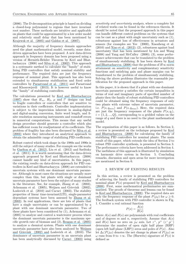
CEAI, Vol.16, No. 3, pp. 84-93, 2014 Printed in Romania A New Data-Driven Approach to Robust PID Controller Synthesis Hossein Parastvand and Mohammad-Javad Khosrowjerdi Department of Electrical Engineering, Sahand University of Technology P.O.Box 51335-1996, Sahand New Town, Tabriz, Iran. (Tel:+984113459369; h [email protected], [email protected]) Abstract: Recently, a new data-driven approach has been proposed for synthesizing the family of stabilizing PID controllers where the proposed approach could not handle any type of uncertainty in the plant model. This paper extends that results to plants with single uncertainty or uncertain plants that can be approximated as plants with a dominant uncertain parameter. It is shown that if an unknown plant with an uncertain parameter satisfies the certain inequalities in terms of real and imaginary parts of the specified plants, then the family of robust stabilizing PID controllers could be obtained using the frequency responses of only two plants corresponding to extreme values of uncertain parameter. No mathematical model is needed and the resulted controller is non-fragile toward its coefficients’ variations. In addition, an exact low frequency band over which the plant data must be known with desired accuracy is sufficient for the controller synthesis and beyond this band the plant data might be approximated. The simulation results on harmonic drive system (HDS) subject to loss of actuator effectiveness show the efficiency of the proposed approach. Keywords: Robust control, PID controller, loss of Effectiveness, data-driven approach, harmonic drive system. 1. INTRODUCTION Controller synthesis without knowing the plant mathemat- ical model is the subject of many studies in the literature. These approaches could be classified in two categories in terms of the data used for synthesis. In the first category, the available information is time domain data and the second category is based on the frequency domain data. Most of data-driven approaches such as adaptive, neural networks and fuzzy methods use time domain information. Various types of fuzzy PID controllers and their devel- opments in achieving auto tuning adaptive and robust capabilities have been reviewed by Malki (1999) and new advancements can be found in ACM (2012) and Zhang and Chang (2012). Tuning the PID coefficients using neural networks is another approach that has been applied by Emilia et al. (2007), Huang (2013) and Lee et al. (2003). A good review of PID tuning techniques has been presented by Bansal et al. (2012). Data-driven controller design using only the frequency response data is one of the current approaches in con- trol literature. The Zigler-Nichols tuning approach that is based on the critical frequency for PID synthesis usually leads to good responses to load disturbances for systems that can be approximated by a first order model with rel- atively small delay; but for more complicated systems the results are not satisfactory. A bunch of frequency domain approaches such as phased locked loop (PLL) by Crowe and Johnson (2001), linear quadratic control algorithm by Kammer et al. (2000) and minimization of the sum of square errors between the desired and measured specifica- tions by Karimi et al. (2003) and Garcia et al. (2006) are all iterative methods that use the Gauss-Newton algorithm and lead to a local optimum of the criteria. Also, they need many experiments on the real system and exact data are needed on the whole range of frequency. Despite its old history, this criteria has not lost its attraction for researchers and over the years new features of frequency response have been released; for example, see Zhou and Hagiwara (2002). In fact, the controller design with minimum knowledge of plant, i.e., the bode or Nyquist diagrams, is the main motivation for control engineers to use these approaches. The frequency response data can be obtained from input-output data using Fourier analysis (Pinelton and Schokens (2001)), virtual sine sweeping (Taghirad (1997)), spectrum analyzer (Petersen and Pota (2003)), network analyzer or using audio sine-wave genera- tors and the sine function of function generators. Sweeping function generators vary (or ”sweep”) their frequency lin- early or exponentially (to give a log plot), and the output amplitude of the swept sine-waves traces the magnitude of the frequency response on an oscilloscope. A slower way of frequency response achievement is through using a fixed-frequency (non-sweeping) sine-wave generator and measuring the output amplitudes at several frequencies with constant input amplitude. Recently, systematic controller design methods in the frequency domain have been developed based on loop- shaping using graphical tools such as bode or Nyquist diagrams by Halikias et al. (2007) that use the concept of quantitative feedback theory (QFT) proposed by Horowitz (2001). Another frequency domain approach based on D- decomposition has been proposed by Gryazina and Polyak
-
Upload
independent -
Category
Documents
-
view
0 -
download
0
Transcript of A New Data Driven Approach to Robust PID Controller Synthesis

CEAI, Vol.16, No. 3, pp. 84-93, 2014 Printed in Romania
A New Data-Driven Approach to RobustPID Controller Synthesis
Hossein Parastvand and Mohammad-Javad Khosrowjerdi
Department of Electrical Engineering, Sahand University of TechnologyP.O.Box 51335-1996, Sahand New Town, Tabriz, Iran.
(Tel:+984113459369; h [email protected], [email protected])
Abstract: Recently, a new data-driven approach has been proposed for synthesizing the familyof stabilizing PID controllers where the proposed approach could not handle any type ofuncertainty in the plant model. This paper extends that results to plants with single uncertaintyor uncertain plants that can be approximated as plants with a dominant uncertain parameter. Itis shown that if an unknown plant with an uncertain parameter satisfies the certain inequalitiesin terms of real and imaginary parts of the specified plants, then the family of robust stabilizingPID controllers could be obtained using the frequency responses of only two plants correspondingto extreme values of uncertain parameter. No mathematical model is needed and the resultedcontroller is non-fragile toward its coefficients’ variations. In addition, an exact low frequencyband over which the plant data must be known with desired accuracy is sufficient for thecontroller synthesis and beyond this band the plant data might be approximated. The simulationresults on harmonic drive system (HDS) subject to loss of actuator effectiveness show theefficiency of the proposed approach.
Keywords: Robust control, PID controller, loss of Effectiveness, data-driven approach,harmonic drive system.
1. INTRODUCTION
Controller synthesis without knowing the plant mathemat-ical model is the subject of many studies in the literature.These approaches could be classified in two categories interms of the data used for synthesis. In the first category,the available information is time domain data and thesecond category is based on the frequency domain data.Most of data-driven approaches such as adaptive, neuralnetworks and fuzzy methods use time domain information.Various types of fuzzy PID controllers and their devel-opments in achieving auto tuning adaptive and robustcapabilities have been reviewed by Malki (1999) and newadvancements can be found in ACM (2012) and Zhangand Chang (2012). Tuning the PID coefficients usingneural networks is another approach that has been appliedby Emilia et al. (2007), Huang (2013) and Lee et al.(2003). A good review of PID tuning techniques has beenpresented by Bansal et al. (2012).
Data-driven controller design using only the frequencyresponse data is one of the current approaches in con-trol literature. The Zigler-Nichols tuning approach that isbased on the critical frequency for PID synthesis usuallyleads to good responses to load disturbances for systemsthat can be approximated by a first order model with rel-atively small delay; but for more complicated systems theresults are not satisfactory. A bunch of frequency domainapproaches such as phased locked loop (PLL) by Croweand Johnson (2001), linear quadratic control algorithmby Kammer et al. (2000) and minimization of the sum ofsquare errors between the desired and measured specifica-tions by Karimi et al. (2003) and Garcia et al. (2006) are
all iterative methods that use the Gauss-Newton algorithmand lead to a local optimum of the criteria. Also, theyneed many experiments on the real system and exact dataare needed on the whole range of frequency. Despite itsold history, this criteria has not lost its attraction forresearchers and over the years new features of frequencyresponse have been released; for example, see Zhou andHagiwara (2002). In fact, the controller design withminimum knowledge of plant, i.e., the bode or Nyquistdiagrams, is the main motivation for control engineers touse these approaches. The frequency response data can beobtained from input-output data using Fourier analysis(Pinelton and Schokens (2001)), virtual sine sweeping(Taghirad (1997)), spectrum analyzer (Petersen and Pota(2003)), network analyzer or using audio sine-wave genera-tors and the sine function of function generators. Sweepingfunction generators vary (or ”sweep”) their frequency lin-early or exponentially (to give a log plot), and the outputamplitude of the swept sine-waves traces the magnitudeof the frequency response on an oscilloscope. A slowerway of frequency response achievement is through usinga fixed-frequency (non-sweeping) sine-wave generator andmeasuring the output amplitudes at several frequencieswith constant input amplitude.
Recently, systematic controller design methods in thefrequency domain have been developed based on loop-shaping using graphical tools such as bode or Nyquistdiagrams by Halikias et al. (2007) that use the concept ofquantitative feedback theory (QFT) proposed by Horowitz(2001). Another frequency domain approach based on D-decomposition has been proposed by Gryazina and Polyak
Control Engineering and Applied Informatics 85
(2006). The D-decomposition principle is based on dividinga closed-loop polynomial to regions that have invariantroot number. These methods are intuitive and applicableon plants that could be approximated by a low order modeland relatively small delay that has been mentioned byKrajewsk et al. (2005) and Galdos et al. (2007).
Although the majority of frequency domain approachesneed the plant mathematical model, recently, some data-driven approaches have been proposed. A new data-drivenapproach in frequency domain has been proposed using aversion of Hermith-Behiler Theorem by Keel and Bhat-tacharyya (2008) and Silva et al. (2002). This approachis a systematic method to calculate the ”family” of stabi-lizing PID controllers that satisfy nominal stability andperformance. The required data are just the frequencyresponse of nominal plant. This approach has also beenextended to simultaneous stabilization and fixed ordercontrollers by Parastvand et al. (2011) and Parastvandand Khosrowjerdi (2013). It is however useful to knowthe ”family” of stabilizing controllers.
The calculations presented by Keel and Bhattacharyya(1997) show that H∞, H2, µ and l1 designs can leadto fragile controllers or controllers that are sensitive tovariations in their coefficients. Controller implementationis subject to the imprecision inherent in analog-digitaland digital-analog conversion, finite word length, and fi-nite resolution measuring instruments and roundoff errorsin numerical computations. This means that any usefuldesign procedure should generate a controller which alsohas sufficient room for readjustment of its coefficients. Theproblem of fragility has also been discussed by Silva et al.(2003) where they introduced an analytical approach toobtain the admissible range of stabilizing PID coefficients.
Robust control which took shape in the 1980s and 1990s isstill the subject of many studies. For example see the worksby Guelton et al. (2012), Liu et al. (2012) and Szelitskyet al. (2011). It is worth mentioning that the data-drivenapproach proposed by Keel and Bhattacharyya (2008)cannot handle any kind of uncertainties. In this paper,the existing results on data-driven approach for PID con-trollers in Keel and Bhattacharyya (2008) are extended touncertain systems with one dominant uncertain parame-ter. Although in most cases the situations are usually morecomplex than this, but plants with single or dominantuncertain parameter have been the subject of many studiesin the literature. See, for example, Zhang et al. (2003),Achemann et al. (2005), Weijnen and Grievink (2002),Loslovich et al. (2010) and Cacuci (2003). The stabilityproperties of linear time-invariant(LTI), single-parameterdependant systems have been assessed by Zhang et al.(2003). In real applications, there are lots of plants thathave a single uncertainty or can be approximated by aplant with one dominant uncertain parameter. Two ofthese plants have been considered by (1), Achemann et al.(2005) to analyze and control a wastewater process wherethe dominant uncertain parameter is the maximum spe-cific growth rate of biomass and (2), Reagan et al. (2005)to analyze a chemical system. Plants with one dominantuncertain parameter have also been analyzed by Weijnenand Grievink (2002) and Loslovich et al. (2010). Thedominance of uncertain parameter in an uncertain planthas been analytically discussed by Cacuci (2003) using
sensitivity and uncertainty analysis, where a complete listof related works can be found in the references therein. Itshould be noted that the proposed approach in this papercan handle different control problems on the systems thatcan be cast as a plant with single uncertainty such as (1),robustness against loss of effectiveness in actuators andsensors (for examples see Yee (2000), Xiaozheng et al.(2010) and Xiao et al. (2012); (2), robustness against loaduncertainty that has been mentioned by Liu and Wang(2008) and Yang and McCalley (2000); (3), some perfor-mance achievements that can be translated to the problemof simultaneously stabilizing. It has been shown by Keeland Bhattacharyya (2008) that the problems ofH∞-normattainment on sensitivity and complementary sensitivityfunctions and satisfying gain and phase margins can betransformed to the problem of simultaneously stabilizing.Solving the above problems illustrates the reasonable jus-tification for the proposed approach in this paper.
In this paper, it is shown that if a plant with one dominantuncertain parameter q satisfies the certain inequalities interms of real and imaginary parts of specified number ofplants then the family of robust stabilizing PID controllerscould be obtained using the frequency responses of onlytwo plants with extreme values of uncertain parameter,i.e. P (s, qmin) and P (s, qmax). Here, the required dataare just the frequency responses of the plants P (s, qi),i = {1, 2, ..., Q}, corresponding to a gridded values on therange of q and there is no need to the plant mathematicalmodel.
The organization of this paper is as follows. In Section 2,a review is presented on the technique proposed by Keeland Bhattacharyya (2008) for calculating the family ofstabilizing PID controllers for nominal plants. The mainresult of this paper, which extends the idea of Section 2 torobust PID controller synthesis, is presented in Section 3.The performance criteria have been addressed in Section 4.The usefulness of this approach is illustrated by simulationon harmonic drive system in Section 5. Concludingremarks, discussion and open areas for more investigationare mentioned in Section 6.
2. REVIEW OF EXISTING RESULTS
In this section, a review is presented on the problemof achieving the family of stabilizing PID controllers fornominal plant P (s) proposed by Keel and Bhattacharyya(2008). First, some mathematical preliminaries are sum-marized. The proofs of theorems and lemma can be foundin Keel and Bhattacharyya (2008). The required data areonly the frequency response of the plant P (jω) for ω ≥ 0.The feedback system with PID controller is shown in Fig.1. Consider a real rational function
P (s) =A(s)
B(s)
where A(s) and B(s) are polynomials with real coefficientsand of degrees m and n, respectively. Assume that A(s)and B(s) have no zero on jω axis. Let z+, p+ (z−,p−)determine the number of open right half plane (RHP)(open left half plane (LHP)) zeros and poles of P (s) . Alsolet ∆∠P (jω) denotes the net change in phase of P (jω) asω runs from 0 to +∞. The (Hurwitz) signature of P (s) isdefined as

86 Control Engineering and Applied Informatics
Fig. 1. The feedback structure of plant with PID
σ(P ) = z− − z+ − (p− − p+) =2
π∆∠P (jω). (1)
Since P (s) has no pole and zero on jω axis, it can bewritten
σ(P ) = −(n−m)− 2(z+ − p+) = −rp − 2(z+ − p+). (2)
The value of z+−p+ can be calculated from Bode diagramof P (s). If P (s) be stable, then z+ can be obtained fromEquation (2). If P (s) be unstable, the frequency responsecould not be achieved directly from the input-outputdata of plant. Let K(s) be a known stabilizing controllerpossibly of high order. Then the frequency response ofunstable plant P (s) can be obtained from
P (jω) =H(jω)
K(jω)(1−K(jω))(3)
where H(jω) is the frequency response of closed looptransfer function.
Theorem 2.1.
z+ =1
2[−rp − rk − 2z+k − σ(H)] (4)
p+ =1
2[σ(P )− σ(H)− rk]− 2z+k (5)
where z+k and rk are the number of RHP zeros and relativedegree of K(s), respectively.
Let P (jω) = Pr(ω)+jPi(ω) where Pr(ω) and Pi(ω) denotethe real and imaginary parts of P (jω), respectively. Letthe real, distinct, finite zeros of Pi(ω) = 0 denote asω0, ω1, ..., ωl−1 such that 0 = ω0 < ω1 < ... < ωl−1. Nowconsider the modified PID controller as
C(s) =ki + kps+ kds
2
s(1 + sT )
where kp, ki and kd are the proportional, integral andderivative coefficients of PID controller and T is a positiveconstant.
Lemma 1. The feedback control system in Fig. 1 is inter-nally stable if and only if the following conditions hold:
(1) There are no pole-zero cancelations in Re(s) ≥ 0when the loop function L(s) is formed.
(2) σ(F̄ (s)) = rp + 2z+ +N , where F̄ (s) = F (s)P (−s).
writeF (ω) = F r(ω, ki, kd) + jωF i(ω, kp)
where
F r(ω, ki, kd) = (ki − kdω2)|P (jω)|2 − ω2TPr(ω) + ωPi(ω)
and
F i(ω, kp) = kp|P (jω)|2 + Pr(ω) + ωPi(ω).
Consider F i(ω, k∗p) = 0 and define
k∗p := g(ω) = −cosφ(ω) + ωT sinφ(ω)
|P (jω)|
=⇒ k∗p := g(ω) = −Pr(ω) + ωTPi(ω)
|P (jω)|2(6)
and J = sgn[F i(∞−, kp)] where kminp < k∗p < kmaxp .
Theorem 2.2. Let ω1 < ω2 < ... < ωl−1 denote the distinctfrequencies of odd multiplicities which are solutions ofF i(ω, kp) = 0. Determine strings of integers
V = [v0, v1, v2, ..., vl]
where vt ∈ {−1, 1} such that: for n−m even:
[v0 − v1 + v2 + ...+ (−1)l−12vl−1 + (−1)lvl](−1)l−1J
= n−m+ 2z+ + 2 (7)
and for n−m odd:
[v0 − v1 + v2 + ...+ (−1)l−12vl−1](−1)l−1J
= n−m+ 2z+ + 2 (8)
and vl = sgn(F r(∞−, ki, kd)). Then for kp = k∗p, thevalues of (ki, kd) corresponding to closed loop stability aregiven by
F r(ωt, ki, kd)vt > 0
=⇒ (ki − kdωt2 −ωt
2Pr − ωtPi|P |2
)vt > 0 (9)
where vt’s are taken from strings satisfying Equations (7)or (8) and ωt’s are taken from the Equation (6).
From the above Theorem the admissible values of (ki, kd)can be determined. Next theorem shows how to calculatethe admissible range of kp.
Theorem 2.3. The necessary condition for PID stabilizingis that there exists admissible range of kp in which thefunction g(ω) has at least R distinct roots of odd multi-plicities such that
R ≥ n−m+ 2z+ + 2
2− 1 : if n−m even
R ≥ n−m+ 2z+ + 3
2− 1 : if n−m odd.
(10)
The procedure for calculating the family of stabilizing PIDcontrollers is summarized in the following algorithm.
Algorithm 1: Calculating the family of stabilizing PIDcontrollers for nominal plant:
Required data: Frequency response or Bode diagram of thenominal plant for ω ≥ 0.
(1) Determine the relative degree rp of P (s) from highfrequency slope of bode magnitude of P (jω).
(2) Determine z+ from (2) or (4).(3) Plot the function g(ω) for ω ≥ 0 from Equation (6).(4) Apply Theorem 2.3 and determine the admissible
range of kp.(5) For kp = k∗p , solve (6) and obtain frequencies of odd
multiplicities as ω1 < ω1 < ... < ωl−1 .(6) Let ω0 = 0 and ωl = ∞ . Determine v0, v1, ..., vl−1
from Equations (7) or (8).(7) For kp = k∗p, determine the (ki, kd) values from
Equation (9).(8) Change the value of kp and go to step 5 to obtain
another stabilizing PID controllers.
3. ROBUST PID SYNTHESIS : A DATA-DRIVENAPPROACH
In this section, the main result of this paper is presented.Consider an uncertain real rational plant P (s, q) as shown

Control Engineering and Applied Informatics 87
Fig. 2. The feedback structure of uncertain plant with PID
in the feedback structure of Fig. 2 where q ∈ [qmin, qmax]is an uncertain parameter. The control objective is tocalculate the family of robust stabilizing PID controllersfor uncertain plant P (s, q). The required data is as follows:
• For stable plants: the frequency spectrum of P (jω, qδ),δ = 1, 2, ..., Q for ω ≥ 0 where Q is the number ofsamples on the gridded range of q.• For unstable plants: the stabilizing controller K(s)
and frequency spectrum of P (jω, qδ) for ω ≥ 0.
Remark 2. The number of samples, i.e. Q, must be highenough so that the set of frequency responses P (jω, qδ)represents an approximation for frequency spectrum ofP (s, q).
The main idea of this section is based on the fact thatif by increasing the uncertain parameter q, g(ω) variesmonotonically, then the following three cases could beverified.
• Case 1: The range of admissible kp for stabilizing theuncertain plant P (s, q) is the common range of ad-missible kp for two plants P (s, qmin) and P (s, qmax).
• Case 2: The inequalities corresponding to P (s, qmin)and P (s, qmax) have the minimum and maximumslope, not necessarily respectively.
• Case 3: The common space of the inequality (9) forP (s, qmin) and P (s, qmax) is a polygon larger thanthe convex region of admissible (ki, kd). A simpleapproach to obtain the exact range of coefficientsmight be vis choosing some test points and analyzingthe stability correspond to. This is needed just at innerpoints of polygon near the vertexes.
An intuitive proof for the above three cases is provided inthe Appendix A.
Thus the key condition for calculating the PID coefficientsis the monotonic varying of g(ω) with increasing theuncertain parameter q. This idea will be used in the nexttheorem to find what kind of systems satisfy this condition.
Theorem 3.1. Let P (jω, qδ), δ = 1, 2, ..., Q be a set offrequency spectrums of an uncertain LTI plant P (s, q)where q ∈ [qmin, qmax] is an uncertain parameter. Thenthe family of stabilizing PID controllers for uncertain plantP (s, q) is a subset of common space between two sets ofstabilizing PID coefficients for P (s, qmin) and P (s, qmax)if the following inequality satisfies for P (jω, qδ) = Pr+jPiand ω ≥ 0
(P 2i + P 2
r + ωPi + Pr)(Pr + ωPi) > 0 . (11)
Proof: From Case 2, if increasing the uncertain parameterleads to monotonic varying the function g(ω), then thefamily of stabilizing PID coefficients for uncertain plantis a subset of common space between two sets of stabi-lizing PID coefficients for P (s, qmin) and P (s, qmax). The
function g(ω) is monotonic if
dg(ω)
dq> 0 or
dg(ω)
dq< 0.
Without loss of generality, consider the case of monotonic
increasing in g(ω), i.e. dg(ω)dq > 0. Increasing the uncertain
parameter leads to increasing in g(ω) if the followinginequality holds
dPr (P 2r −P 2
i + 2ωPrPi) + dPi (P 2i ω−P 2
r ω+ 2PrPi) > 0 .(12)
To obtain the solution, it is needed to apply some divisionsduring solving the above differential inequality. These di-visions might change the real rational symbol of inequality(i.e. the symbol ’>’). For the sake of simplicity, the aboveinequality will be solved as an equality, and at the end,the effects of divisions on the real rational symbol of thefinal results will be considered. Therefore, the followingequation must be solved
dPr (P 2r − P 2
i + 2ωPrPi) + dPi (P 2i ω − P 2
r ω + 2PrPi) = 0.(13)
By dividing the above equation on
α := P 2i ω − P 2
r ω + 2PrPi, (14)
it can be writtendPidPr
=P 2i − P 2
r − 2ωPrPi
P 2i ω − P 2
r ω + 2PrPi. (15)
Through change of variable as z = Pi
Pr, the above equation
transforms to
Pr dz =−z3ω − z2 − zω − 1
z2ω + 2z − ωdPr . (16)
To obtain a homogeneous differential equation, both sidesof Equation (16) are devided by
β := Pr, (17)
and
γ :=−z3ω − z2 − zω − 1
z2ω − ω + 2z. (18)
As a result, the Equation (16) could be transformed to
z2ω + 2z − w−z3ω − z2 − zω − 1
dz =1
PrdPr
⇒ (−2z
z2 + 1+
−ω−zω − 1
) dz =1
PrdPr ⇒ ln(
−zω − 1
(z2 + 1)Pr) = 0,
⇒ −zω − 1
(z2 + 1)Pr= 1, (19)
and by substituting z = Pi
Pr, one can write
P 2i + P 2
r + ωPi + Pr = 0. (20)
Now the real rational symbol of above equation could beobtained by considering the effect of divisions on (14), (17)and (18), i.e. terms α, β and γ. Obviously the real rationalsymbol of the resulted equation in (20) is dependent to thesign of the multiplication of (αβγ). Then, it can be written{
If αβγ > 0 then P 2i + P 2
r + ωPi + Pr < 0,If αβγ < 0 then P 2
i + P 2r + ωPi + Pr > 0 .
(21)
On the other side, from the multiplication of (αβγ) as
αβγ = (P 2i ω − P 2
r ω + 2PrPi)Pr(−z3ω − z2 − zω − 1
z2ω − ω + 2z),
and by substitution z = Pi
Prit can be written{
for αβγ > 0 then − (Pr + ωPi) > 0,for αβγ < 0 then − (Pr + ωPi) < 0 .
(22)

88 Control Engineering and Applied Informatics
The combination of two sets of inequalities in (21) and (22)leads to (11). Similarly, the same results can be obtained
for dg(ω)dq < 0 . 2
Remark 3. Thanks to Theorem 3.1, the class of systemsthat proposed data-driven approach could deal with can bedefined. In fact, the class of systems that can be addressedby the proposed approach of this paper must satisfy thefollowing conditions
I. The inequality (11) should be hold at each frequencyω ≥ 0 for P (jω, qδ),
II. There should be a common range between admissiblekp for P (s, qmin) and P (s, qmax).
Remark 4. The frequency response data corresponding toP (s, qmin) and P (s, qmax) could be recognized from theset of frequency responses of uncertain plant P (jω, q). Infact if the inequality (11) holds, then it could be deducedthat the uppermost and lowermost plots of g(ω) are cor-responding to P (s, qmin) and P (s, qmax), not necessarilyrespectively.
Remark 5. It worth mentioning that almost in every appli-cation the set of ωt
′s can be found in the low frequencies.This means that only an exact data of the low frequencyband is sufficient for controller synthesis and beyond thisband the plant information may be rough or approxi-mated.
The procedure for calculating the family of stabilizing PIDcontrollers is summarized in the following algorithm.
Algorithm 2: Calculating the family of stabilizing PIDcontrollers for uncertain plant P (s, q) in which q ∈[qmin, qmax] is an uncertain parameter
Required data: P (jω, qδ) for δ = 1, 2, ..., Q and ω ≥ 0.
(1) Check the inequality (11). If this inequality holds thengo to the next step.
(2) Determine the extreme plots of g(ω) correspond toP (jω, qmin) and P (jω, qmax) using Remark 4.
(3) Apply Theorem 2.3 to obtain the common set ofadmissible kp for two plants found in the previousstep.
(4) Using Steps 5-8 of Algorithm 2 determine the set of(ki, kd) coefficients for P (jω, qmin) and P (jω, qmax).
(5) Calculate the common range of (ki, kd) coefficientsbetween P (jω, qmin) and P (jω, qmax).
(6) Calculate the exact family of admissible (ki, kd) usingthe approach proposed in Case 3.
4. PERFORMANCE ACHIEVEMENT
Many performance achievement problems for plant P (s)can be cast as the simultaneously stabilization of plantand the family of real and complex plants. Some ofthese performance achievement problems are listed in Keeland Bhattacharyya (2008). For example the problem ofH∞-norm achievement on the complementary sensitivityfunction is equivalent to simultaneously stabilizing theplant P (s) and the family of real plants
PC(s) =[1 +
1
γejθW (s)
]P (s) : θ ∈ [0, 2π]
where γ is an arbitrary parameter and W (s) is the optionalweighting function. The above function represents a plant
Fig. 3. The feedback structure of plant faced to loss ofactuator effectiveness with PID
with an uncertain parameter θ. So the proposed approachin this paper can be effectively applied here to obtain thefamily of stabilizing plants that satisfy H∞-norm on thecomplementary sensitivity function. The same criteria hasbeen used for satisfying desired gain and phase marginsand H∞-norm specification on the sensitivity function byKeel and Bhattacharyya (2008).
Remark 6. Assume that P (s, q) be a plant with an uncer-tain parameter q. Let PC(s, q, θ) be a plant with anothervirtual uncertain parameter θ corresponding to above per-formance specification parameters. If necessary conditionsof Theorem 3.1 satisfy for both P (s, q) and PC(s, q∗, θ)where q∗ belongs to {qmin, qmax}, then the family of PIDcontrollers that achieve the above performance specifica-tions for uncertain plant P (s, q) is the subset of stabilizingPID coefficients for
PC(s, q, θ) : q = {qmin, qmax}, θ = {0, 2π}.
The approach can handle different control problems thatcan be evaluated as a plant with an uncertain parame-ter. For example, the problem of controller synthesis fordifferent types of electrical machines, such as, DC motor,induction motor, synchronous motor, etc that are faced toload uncertainty mentioned in Liu and Wang (2008) canbe cast as a plant with an uncertain parameter, in whichthe uncertain parameter q is the uncertain load.
5. SIMULATION RESULTS
In this section, an example is presented to show theusefulness of the proposed approach. In this example, theproblem of controller synthesis for a harmonic drive system(HDS) faced to loss of actuator effectiveness has beenaddressed. Loss of actuator effectiveness is an importantproblem from practical point of view. See, for example,Yee (2000) and Xiao et al. (2012). Fig. 3 might representthe feedback structure of an uncertain plant with PIDcontroller faced to loss of actuator effectiveness whereq = L is the uncertain parameter corresponding to lossof effectiveness and belongs to (0,1]. A similar case willhappen when there is a loss in sensor effectiveness. Thus,using Algorithm 2, the family of robust PID controllers forplants faced to loss of actuator/sensor effectiveness can becalculated.
The frequency response of the HDS is shown in Fig. 4that is calculated by Taghirad (1997) using virtual sinesweeping (VSS). Here the control objectives are

Control Engineering and Applied Informatics 89
−80
−60
−40
−20
0
20
Magnitude (
dB
)
100
101
102
103
104
−180
−135
−90
−45
0
Phase (
deg)
Bode Diagram
Frequency (rad/sec)
Fig. 4. The Bode diagram of HDS with L = 1
Fig. 5. The plot of function g(ω) for HDS with L = 1
(1) Calculating the family of stabilizing PIDs for nominalplant, i.e P (s, L) where L = 1.
(2) Calculating the family of stabilizing PIDs that satisfyH∞-norm on complementary sensitivity function fornominal plant.
(3) Satisfying the previous performance criterion for theHDS faced to loss of effectiveness in actuator, i.e. forthe plant P (s, L) where 0 < L ≤ 1.
First consider the case where there is not loss of actuatoreffectiveness, i.e. L = 1. The corresponding function g(ω)is shown in Fig. 5. So the admissible range of kp is[−1,+∞). Calculating the (ki, kd) values for kp = 10 isresulted to the following inequalities
ki > 0ki < 722kd + 497.
The whole range of stabilizing PID coefficients is shown inFig. 6.
Now consider the problem of H∞-norm achievement onthe complementary sensitivity function. The range of(ki, kd) that satisfies this performance criterion for kp = 10
Fig. 6. The whole family of stabilizing PID controllers forHDS with L = 1
Fig. 7. Admissible ranges of ki − kd that satisfy stabilityand performance for HDS with L = 1 and kp = 10
−100
−80
−60
−40
−20
0
20
Magnitude (
dB
)
100
101
102
103
104
−180
−135
−90
−45
0
Phase (
deg)
Bode Diagram
Frequency (rad/sec)
Fig. 8. bode diagram of HDS with L = {0.01, 0.4, 0.7, 1}

90 Control Engineering and Applied Informatics
Fig. 9. (ki, kd) values for kp = 10 of only stabilizingcontrollers, controllers satisfy H∞ performance andcontrollers satisfy H∞ performance at the presence ofloss of actuator effectiveness
Fig. 10. The family of robust PID controllers for HDS
is shown in Fig. 7. The whole range of (ki, kd) could beobtained similarly.
Now, if the loss of actuator effectiveness happens, itcan be inferred from Section 3 that the HDS with thisphenomenon is an special case of a plant with an uncertainparameter. Therefore, the proposed approach could beapplied for such systems. Figure 8 shows the effect of lossof actuator effectiveness for L = {0.01, 0.4, 0.7, 1} on themagnitude of Bode diagrams of HDS. Simulation resultsshow that the conditions of Remark 6 satisfy; thus therobust PID controllers can be calculated by simultaneouslystabilizing of two plants P (s, Lmin) = P (s, 0.01) andP (s, Lmax) = P (s, 1).
The range of (ki, kd) values for kp = 10 that achieveto stability and performance in the presence of loss ofactuator effectiveness is shown in Fig. 9 and the wholerange is obtained in Fig. 10 by sweeping on kp. The stepresponses of plant is shown in Fig. 11 when the value ofloss of actuator effectiveness is set to L = 0.1. As shown inFig. 11, the step response of robust PID controller applied
to HDS has the best transient response in comparison withcontrollers that satisfies nominal stability and nominalperformance. The corresponding control inputs is shownin Fig. 12.
Although the example provided here considers the gainuncertainty which is rather a trivial case, but some argu-ments and examples are provided by Parastvand (2010)that imply this condition can be satisfied satisfied for alarge class of industrial processes.
6. CONCLUSION AND DISCUSSION
This paper provided an extension of a data driven con-troller synthesis from nominal stability to robust stabilityand performance. It is shown that for an unknown plantwith a single or dominant uncertain parameter, if somesmooth conditions hold, then the family of stabilizing PIDcontrollers corresponding to two plants with extreme val-ues of uncertain parameter can guarantee robust stabilityfor all perturbed plants with any value of uncertaintybetween those two extremes. The required data are thespecific number of frequency responses of plants corre-sponding to the gridded values of uncertain parameter.There is no need to exact frequency responses on the wholefrequencies, and only accurate data on the low frequencyband is sufficient in almost any application. Also it is illus-trated that some control problems such as achieving theperformance specifications, robustness against loss of effec-tiveness in actuator and load uncertainty can be charac-terized as the problem of robust stabilizing of a plant withan uncertain parameter. Another feature of the proposedtechnique is the non-fragility of the obtained controller orcontroller robustness because of existing a reliable bandfor admissible PID coefficients. The proposed approach issuccessfully simulated on harmonic drive system faced toloss of effectiveness.
The presented method can easily be extended to model-based synthesis. Some plants that are faced to parametersvariations can be approximated by plants with a domi-nant uncertain parameter. From this point of view, theproposed approach can be used for model-based uncertainsystems to calculate the family of robust stabilizing PIDcontrollers. Also, the proposed approach could be easilyextended to time-delay systems using some modificationson the approach proposed in Keel and Bhattacharyya(2008). The open areas of research under study are (a), thedesign of such controllers for multivariable and nonlinearplants, and (b), developing the proposed approach to otherstructured and unstructured uncertainties.
ACKNOWLEDGMENT
This work has been carried in Advanced Control ResearchLaboratory(ACRL) in the Sahand University of Technol-ogy (SUT).
Appendix A
Here are the proof of three cases presented in Section 3.The proof for Case 1 is obvious. For Case 2, we know thatthe slope of inequalities of Equation (9) is equal to ω2
t .The values of ωt for every q can be obtained from g(ω) for

Control Engineering and Applied Informatics 91
Fig. 11. Step responses of HDS system with PID
Fig. 12. Control inputs of HDS system with PID
k∗p. Now if by changing the q, g(ω) varies monotonically
then the maximum and minimum values of ω2t would be
obtained for qmin and qmax in P (s, qmin) and P (s, qmax).Then, the maximum and minimum slope of inequalitiesin (9) correspond to P (s, qmin) and P (s, qmax). In Fig.A.1, the plot of inequalities corresponding to Equation(9) is shown for some values of uncertain parameter q fora typical example. As shown in Fig. A.1, the admissiblevalues for (ki, kd) are a subset of inequalities obtained fromEquation (9) for P (s, qmin) and P (s, qmax). For Case 3,let by monotonic varying in q, g(ω) varies monotonically.This leads to monotonic varying in the slope of inequalities(9). Now, if the values of y-intercepts vary in the samemanner, then the common space of inequalities (9) forP (s, qδ), δ = 1, 2, , Q, is exactly equal to the commonspace of just two plants P (s, qmin) and P (s, qmax). Butthis is the case that can not be guaranteed. In the otherword, since the values of y-intercepts of the lines obtainedfrom (9) are different, the common space of the inequalities(9) for P (s, qδ) is smaller than the common space of justtwo plants P (s, qmin) and P (s, qmax). This can be seen
from Fig. A.1. In spite of the fact that two green trianglesbelong to admissible range of (ki, kd) for P (s, qmin) andP (s, qmax), but they do not belong to admissible range of(ki, kd) for P (s, q). To obtain the exact family of stabilizingPID coefficients, the shadowed region in Fig. A.1 must beexcluded. One simple approach to exclude the shadowedregions is to choose some test points in these regions andanalyze the stability correspond to.
REFERENCES
ACM (2012), “Advances in Fuzzy Systems, Special issueon Fuzzy Function, Relations, and Fuzzy Transforms,”Advances in Fuzzy Systems, Hindawi Publishing Corp.,New York, NY, United States, vol. 2012.
Aschemann, H., Rauh, A., Kletting, M., Hofer, E.P, Gen-nat, M. & Tibken, B. (2005), “Interval analysis andnonlinear control of wastewater plants with parameteruncertainty,” IFAC World Congress, Czech Republic,pp. 2179-2185.
Bansal, H.O., Sharma, R. & Shreeraman, P.R. (2012),“PID Controller Tuning Techniques: A Review,” Jour-

92 Control Engineering and Applied Informatics
Fig. A.1. The plot of inequalities obtained from Equation(9) for k∗p for a typical example
nal of Control Engineering and Technology, vol. 2, no.4, pp. 168–176.
Cacuci, D.G. (2003), “Sensitivity and uncertainty AnalysisTheory,” Chapman & Hall/CRC.
Crowe, J. & Johnson, M.A. (2001), “Automated PI controltuning to meet classical performance specifications usinga phase locked loop identifier,” In IEEE AmericanControl Conference, Arlington, USA, pp. 21862191.
Dehghani, A., Lecchini, A., Lanzon, A. and Anderson,B.D.O. (2009), “Validating Controllers for Internal Sta-bility Utilizing Closed-Loop Data,” IEEE trans. Au-tomat. Control, vol. 54, pp. 2719-2725.
D’Emilia, G., Marra, A., and Natale, E. (2007), “Use ofNeural Networks for Quick and Accurate auto-tuningof PID Controller,” Robotics and Computer-IntegratedManufacturing, vol. 23, pp. 170-179.
Galdos, G., Karimi, A. & Longchamp, R. (2007), “Robustloop shaping controller design for spectral models byquadratic programming,” In 46th IEEE conference ondecision and control, New Orleans, USA, pp. 171–176.
Garcia, D., Karimi, A. & Longchamp, R. (2006), “Data-driven controller tuning using frequency domain specifi-cations,” Industrial & Engineering Chemistry Research,vol. 45, no. 12, pp. 40324042.
Gryazina, E.N. & Polyak, B.T. (2006), “Stability regionsin the parameter space: D-decomposition revisited,”Automatica, vol. 42, no.1, pp. 13–26.
Guelton, K., Jabri, D., Manamanni, N., Jaadari, A., &Chinh, C.D. (2012), “Robust stabilization of nonlinearsystems based on a switched fuzzy control law,” Journalof Control Engineering and Applied Infoormatics, vol.14, no. 2, pp. 40-49.
Halikias, G.D., Zolotas, A.C. & Pota, Nandakumar, R.(2007), “Design of optimal robust fixed structure con-trollers using the quantitative feedback theory ap-proach,” IMechE / Professional Engineering Publish-ing,.
Horowitz, I.M. (2001), “Survey of quantitative feedbacktheory (QFT),” International Journal of Robust andNonlinear Control., vol. 11, pp. 887–921.
Huang, C. P. (2013), “Stability analysis and controllersynthesis for fuzzy descriptor systems”, InternationalJournal of Systems Science, vol. 44, no. 1, pp. 23-33.
Kammer, L.C., Bitmead, R.R & Bartlett, P.L. (2000), “Di-rect iterative tuning via spectral analysis,” Automatica,vol. 36, no. 9, pp. 13011307.
Karimi, A. Garcia, D. & Longchamp, R. (2003), “PIDcontroller tuning using Bodes integrals, IEEE Transac-tions on Control Systems Technology, vol. 11, no. 6, pp.812821.
Keel, L.H. & Bhattacharyya, S.P. (2008), “Controller syn-thesis free of analytical model: Three term controllers,”IEEE trans. Automat. Control, vol. 42, no.8, pp. 1098–1105.
Keel, L.H. & Bhattacharyya, S.P. (1997), “Robust, Fragile,or Optimal?,” IEEE trans. Automat. Control, vol. 53,no.6, pp. 1353–1369.
Krajewsk, W., Lepschy, A., Miani, S. & Viaro, U. (2005),“Freaquency-domain approach to robust PI control,”Journal of Franklin Institue., vol. 342, no. 6, pp. 674–687.
Lee, C.H. & Teng, C.C. (2003), “Calculation of PIDParameters by Using a Fuzzy Neural Network” ISATransaction, vol. 42, no. 2, pp. 391-400.
Liu, X, Feng, S, and Ma, M. (2012), “Robust MPC forthe constrained system with polytopic uncertainty”,International Journal of Systems Science, 43(2), 248-258.
Liu, Z. & Wang, Q. (2008), “Robust control of electricalmachine with load uncertainty,” Journal of ElectricalEngineering, vol. 59, no. 2, pp. 110–112.
Loslovich, I., Moran, M.I. & Gutman, P. (2010), “Identi-fication of a nonlinear dynamic biological model usingthe dominant parameter selection method,”Journal ofFranklin Institue, vol. 347, no. 6, pp. 1001-1014.
Malki, H. A. (1999), “Fuzzy Theory Systems: Techniquesand Applications” Elsevier Inc., vol.2, Chap.22, pp. 609-629.
Parastvand, H. (2010), “Controller synthesis free of analyt-ical model: Frequency domain approaches,” MSc Thesis,Sahand University of Technology, Tabriz, Iran.
Parastvand, H., Khosrowjerdi, M. J., & Akbari Alvnagh,A. (2011), “A new model-free approach to simultane-ously stabilizing,” The 19th Iranian Conference on Elec-trical Engineering(ICEE), Tehran, Iran.
Parastvand, H. & Khosrowjerdi, M. J. (in press,published online: 09 Jul 2013), “Controller syn-thesis free of analytical model: fixedorder con-trollers,” International Journal of Systems Science,doi:10.1080/00207721.2013.815823.
Petersen, I.R. & Pota, H.R. (2003), “Minimax LQG op-timal control of a flexible beam,” Control EngineeringPractice., vol. 11, pp. 1273–1287.
Pinelton, R. & schoukens, J. (2001), System identification:a frequency domain approach, Newyork, USA: IEEEpress, .
Reagan, M.T., Najm, H. N., Pebay, P.P., Knio, O.M.& Ghanem, R.G. (2005), “ Quantifying uncertainty inchemical systems modeling, International Journal ofChemical Kinetics, vol. 37, no. 6, pp. 368-382.
Silva, G.J., Datta, A., & Bhattacharyya, S.P. (2003),“On the Stability and Controller Robustness of SomePopular PID Tuning Rules,” IEEE trans. Automat.

Control Engineering and Applied Informatics 93
Control, vol. 48, no.9, pp. 1638–1641.Silva, G.J., Datta, A., & Bhattacharyya, S.P. (2002), “New
result on the synthesis of PID controllers,” IEEE trans.Automatic Control, vol. 47, no. 2, pp. 241–252.
Szelitsky, T., Inoan, I., & Dumitrache, D.C., (2011), “Ad-vantages of Robust Control for Series Load FrequencyControlled Induction Heating Inverters,” IinternationalJournal of Control Engineering and Applied Informat-ics, vol. 13, no. 1, pp. 54-61.
Taghirad, H.D. (1997), Robust control of harmonic drivesystem, Ph.D. dissertation, Dept. Electrical Engineer-ing, McGill University, Montreal.
Weijnen, & Grievink, J. (2002), “Hierarchical Approachfor Selecting Uncertain Parameters at the ConceptualStage of Design,” In European Symposium on ComputerAided Process Engineering, 199–204.
Xiao, B., Hu, Q. & Friswell, M.I. (2012), “Active fault-tolerant attitude control for flexible spacecraft withloss of actuator effectiveness,” International Journal ofAdaptive Control and Signal Processing, First publishedonline.
Xiaozheng, J., Guanghong, Y. & Yanping, L. (2010),“Robust fault-tolerant controller design for linear time-invariant systems with actuator failures: an indirectadaptive method,” Journal of Control Theory Applica-tions, vol. 8, no. 4, pp. 471–478.
Yang, N. & McCalley, J.D. (2000), “-analysis and synthesisfor the uncertainties in static load modeling,” ElectricPower Systems Research, vol. 56, no. 1, pp. 17-25.
Yee, J.S. (2000), “Resilient H∞ controller design to toler-ate loss of actuator effectiveness for discrete-time uncer-tain linear systems” American Control Conference, vol.4, pp. 2443–2447.
Zhang, X., & Chang, B. (2012), “Design of Water-savingIrrigation Monitoring System Based on CC2430 andFuzzy-PID,” Journal of Control Engineering and Tech-nology, vol. 2, no.3, pp. 124–129.
Zhang, X., Tsiotras, P. & Iwasaki, T. (2003), “Parameter-dependent Lyapunov function for exact stability anal-ysis of single-parameter dependent LTI systems,” Pro-ceedings. 42nd IEEE Conference on Decision and Con-trol, vol. 5, pp. 5168–5173.
Zhou, J, and Hagiwara, T. (2002) , “Existence Conditionsand Properties of the Frequency Response Operators ofContinuous-Time Periodic Systems”, SIAM Journal onControl and Optimization , (40)6, 18671887.