An expert PID controller uses refined ziegler and nichols rules and fuzzy logic ideas

Journal of Applied Intelligence 4, 53-66 (1994) © 1994 Kluwer Academic Publishers, Boston. Manufactured in The Netherlands.

An Expert PID Controller Uses Refined Ziegler and Nichols Rules and Fuzzy Logic Ideas

GERARDO GABRIEL ACOSTA Universidad de Valladolid, Facultad de Ciencias, Departamento de Informdtica, Prado de la Magdalena s/n,

(47011) Valladolid, Spain ComisiOn de Investigaciones Cientificas de la Provincia de Buenos Aires (CICpBA), Argentina

M1GUEL ANGEL MAYOSKY ComisiOn de Investigaciones Cientificas de la Provincia de Buenos Aires (C1CpBA), Argentina

JOSt~ MARIA CATALFO Consejo Nacional de Investigaciones Cientificas y T6cnicas (CONICET), Argentina

ACOSTA@SUN. AUTO. ISA .CIE. UVA.ES

Received June 1, 1992; revised August 6, 1993

Abstract. This article proposes a scheme for the on-line adjustment of three mode controller settings based on experimental measurements of closed-loop performance. It uses a recently developed heuristic tuning procedure to identify estimated process parameters. This method may give rise to conflicting estimates. Fuzzy Set theory is applied to manage the situation in terms of a fuzzy conjunction to combine the various estimates. PID control was chosen because of its wide use in the industrial environment due to driving simplicity and robustness. The article shows design, development, and computer simulation aspects.

Key words: PID control, fuzzy logic, pattern recognition, expert system

1. Introduction

The PID (proportional, integral, derivative) is a widely used closed-loop controller in industrial environments. It is simple and easy to carry out, and its design does not require an exact knowledge of the controlled plant's dynamics. Many heuristic methods exist to determine the algorithm's coefficients for a wide range of typical industrial processes. The well-known Ziegler and Nichols rule [1] provides such a heuristic procedure for sigmoid-type step response plants. These plants have a step response curve like that shown in figure 1. Although these processes have several time constants (most industrial processes are multicapacity, so they have an integrative behavior), they can be reduced to a dead time plus

a single capacity [2]. Then, the plant input-output relation is given by

k x e -~×~ Gp(~)- a x s + 1 [l]

where

-r: a pure time delay k: process gain a: process time constant

Several approaches have been made in recent years for the automatic tuning of PID controllers. Among others, relay feedback [3], approximate system identification [4], cross correlation [5], and Expert Systems [6, 7], provide ways to find near-optimal settings for the controller parameters.

54 Acosta, Mayosky and Catalfo

Process Output

O.200"65 . . . . . . . . . . . . . . . . . . .

0,00 I II Tau time

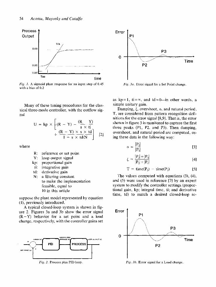
Fig. 1. A sigmoid plant response for an input s tep of 0.45 with a bias of 0.2

Error P1

\

P2

Fig. 3a. Error signal for a Set Point change.

m

Time

Many of these tuning procedures for the classical three-mode controller, with the outflow signal

(R - Y) U = kp x ( R - Y) + s x ti

where

( R - Y) x s x td] +

1 - + s x td/N J [2]

R: reference or Set point Y: loop output signal

kp: proportional gain ti: integrative gain

td: derivative gain N: a filtering constant

to make the implementation feasible, equal to 10 in this article

suppose the plant model represented by equation (1), previously introduced.

A typical closed-loop system is shown in figure 2. Figures 3a and 3b show the error signal ( R - Y ) behavior for a set point and a load change, respectively, with the controller gains set

MANIPULATED ERROR (el W, RIABLE (u) LOOP OUTPUT {¥1

•

SET POINT

Fig. 2. Process plus PID loop.

as kp= 1, t i = % and td=0---in other words, a simple unitary gain.

Damping, ~, overshoot, o, and natural period, T, are considered from pattern recognition defi- nitions for the error signal [8,9]. That is, the error shown in figure 3 is monitored to capture the first three peaks (P1, P2, and P3). Then damping, overshoot, and natural period are computed, using these data in the following way:

IP21 o = led [3]

I P z I + I P ~ I

¢ -- ]P21 + [ P , I [4]

T = time(P3) - time(P1) [5]

The values computed with equations (3), (4), and (5) were used in reference [7] by an expert system to modify the controller settings (proportional gain, kp; integral time, ti; and derivative time, td) to match a desired closed-loop re-

Error

0

Pl

/ \ , 3

Time

P2

Fig. 3b. Error signal for a Load change.

An Expert PID Controller 55

sponse. It can be qualified based on performance criteria such as, among others,

ITAE: (Integrated Time Absolute Error) t

= / l e l × t x dt [6] 0

ISE: (Integrated Square Error) t

= ( e 2 × d t [7] 0

IAE: (Integrated Absolute Error) t

= / [ e I x dt [8] 0

which take into account the error evolution. In our case, the PID controller we used has a

gain ranger (figure 4, 13) to weigh the reference. The advantage of this set point filtering is to obtain a different system response for set point changes than for load changes [10, 11]. It is known that often the Ziegler and Nichols rules give an excessive closed-loop overshoot to a step input. However, they provide a good response to a load perturbation.

Therefore, the control signal given by the PID can now be described by the following equation:

U = kp × [([3 x R - Y) L

( R - Y) (Y) x s x td ] +

s x ti 1 + s x td/N] [9]

where (R - Y) is again the error and 13 is the reference wieghting factor. Note, by comparing equations (9) and (2), that not only the weighted reference feature was added, but also the predic- tive term (derivative) in equation (9) gets its input information from the loop output Y, instead of getting it from the error, as in equation (2). By so doing, the new PID structure is faster.

Some refinements of the Ziegler and Nichols tuning formula [12], proposed for the PID structure of equation (9), are used in this article. They are intended to reduce overshoot due to set point changes and to improve the total response for plants with large normalized delays.

Following [12], a heuristic process characterization can be defined by

where

K: kss: k~:

O: 'r: a:

K = k++ × k. [10a]

® = -r/a [t0b]

normalized process gain, process steady-state gain, process ultimate gain,

normalized dead-time, apparent dead-time, apparent time constant of the open-loop process' step response.

Equations (10a) and (10b) are empirically re- lated by

K = 2 × 37 × ® - ' [11]

+ ,[ ko tO s ti

+()_[ kp SE

I I -kp td s

l+s td/N

t

,?- 0 + TO PROCESS (u) ÷

D +l ]

FROM LOOP OUTPUT (y)

q

Fig. 4. Modified PID s t ructure for a weighted reference.


Equation (11) represents a hyperbola. Thus, the definition of normalized gain has no real value for normalized delays tending to zero. Going further, in such a situation, we would have a first-order process, and we would need an ultimate gain (ku) tending to infinity to obtain a rea- sonable normalized gain. Since it is impossible to define an ultimate gain for a first-order process, the characterization recently proposed is accord- ing to the classical control theory. Then, it is meaningless to consider normalized delays near zero. For the present application, normalized delays lower than or equal to 4/37 are not considered.

Finally, the recommended PID parameters' values can be stated as a function of (9, K, ku, and tu (the ultimate time, corresponding to ko, the ultimate gain).

Once this tuning is done, the expert controller should continue with the loop response observation and, if necessary, change the PID parameters' values [7].

The main contribution of our present approach is • link the observed pattern of the closed-loop re-

sponse (characterized by 4, o, and T), with (9 and K to estimate the appropriate initial PID parameters set; and

• use Fuzzy Set Theory to combine the various estimates. This is done with expert rules.

The article also includes simulation results for some case studies as well as our conclusions.

2. Observed Pattern and Process Characterization

Analyzing the closed-loop step response of the process represented by equation (1), in the se- quel Process 1, over a great deal of computer simulations, with k= 1, kp= 1, t i=~ , and td=0, we could obtain a relationship between overshoot, o, damping, 4, natural period, T, and normalized dead-time, ® (see figures 5a, 5b, and 5c).

Overshoot, damping, and natural period were defined [9] as relations among the three first peaks of the time response. When there are no peaks, the system assumes default values and manages the situation to create them. For nor-

malized delays tending to zero, the process of equation (1) tends to a first-order one, as was said in a preceding paragraph. This process, in closed-loop with a proportional controller, does not give overshoot for set-point changes, as shown in figure 5, where the default values are an overshoot of 0.5, a damping of 0.67, and a natural period of 50.

Similar curves to the ones obtained for normalized dead-time can also be obtained for the normalized process gain, K, using equation (11). They are encoded in the controller's knowledge base together with the procedures that handle them. This response evaluation allows an empirical process identification used for the controller on-line tuning.

The entire system is shown in figure 6. It com- prises the process described by equation (1) and an expert system that does the heuristic identification and then supplies the PID parameters, in this case kp, ti, td, and [3, from the observed error pattern.

0.55

0,5

0.45

0.4

0.35

03

0'25 1 \, 0.2

0.~ 022 o14 o16 ols 1 ~I~ ;~ 11~ A

Fig. 5a. Overshoot variation with the normalized delay (0).


0.78 i i

0.76 i

0.74

0.72

0.7 /

0'660~

0.64 , , i 012 014 016 0,8 1 112 114 116 118 2 Norm*li~ l~lry

Fig. 5b. Damping variation with the normalized delay (0).

50 - - ~

45

40

35

l

30;

25F

2op

t5 i !

11, [ f J J ~

%[ 012 014 016 018 1 112 114 116 1 1 8 - -

Fig. 5c. Natural period variation with the normalized delay (o).

3. Control Strategy

We organized the control strategy in two main parts: l) an identification stage, and 2) a supervisory stage.

3.1. Identification Stage

At startup, the self-tuning controller captures the loop response pattern caused by a known input

(a limited amplitude step sequence), superim- posed onto the usual loop reference.

The first step in the sequence is used to obtain the loop steady gain k+s and the parameters @ and K in terms of overshoot, damping, and natural period. Uncertainty arises when using the curves shown in figures 5 to perform this task, as will be seen in section 4. Once we obtain K and ks+, we can compute the ultimate gain ku (see equation (lOa)).

SET POINT (r) ERROR (e) +

,( -[ MANLPULATED

VARIABLE (u) LOOP OUTPUT [PROCESS] I '

Fig. 6. The whole system.

(y)


In the second step, the controller gain is set to ku in order to obtain the ultimate period tu, using the .A, strom and Hagglund method [3]. This method produces a limited oscillation, as small as the situation accepts, and does not at all imply that the process should be carried to critical operation conditions. This situation, of course, may be intolerable in many industrial processes (i.e., highly exothermic reactors).

After these presets, we have enough information to apply the heuristic rules [12] and get the first PID parameter set. The [3 block is adjusted in this work for a 10% overshoot in the time response.

3.2. Supervision Stage

Once the loop is working, it may be necessary to do a supplementary on-line tuning of the PID parameters. This is due to the low-order process characterization we have done using the normalized dead time and gain, and/or changes in the plant model. Moreover, perturbations are usually other than steps, and the expert system must take this into account.

4. Embedding Fuzzy Ideas in the Knowledge Base

The utilization of fuzzy logic in process control is not new [13-15]. Although it is not the purpose of this article to provide the fundamentals of fuzzy logic, which may be found in other works [16, 17], we shall briefly explain them whenever it becomes necessary.

Fuzzy logic is a formal frame to manage un- certain knowledge or, in other words, a theory for approximate reasoning. This reasoning is fre- quently used by human beings. When trying to embody a human operator's expertise or even a simple commonsense knowledge in an expert system, this tool seems very attractive and useful. Both features are applied not only to repre- sent facts but also to reason with them.

In process control, even when the best controller could be designed, usually the plant startup and the final on-line tuning are left to the control engineer or the expert operator, because the plant model is usually linearized around the working point.

In our present problem, as we said before, there are some sources of approximate knowledge. One of them is the process identification. The curves in figure 5 are empirical laws obtained from the simple observation of the loop response. When using them, it is almost never the case that the final normalized dead-time value is the same for the three curves. To be more precise, suppose that observing the loop response under the conditions established in step 3.1, the following characterization parameters are obtained:

~j for the damping

% for the overshoot

Tj for the natural period

The system then queries the knowledge base, and a situation like that shown in figure 7 is reached, where ®~j # ®oj ~ ®vj-

The question now is, which is the real value of ®j? We propose to reason in the following way: each curve is a different source of knowledge. A priori, we believe the information from each of

50 ........... ----,-.

g 30

©

e -,~, 20

e~

10

7"j o

i

O iT

". ,,,

' , , , '-.,

"''.,,.,

"'"....

o,o 0.8 1 1.2 1.4 1,6 1.8

Normalised Delay 0

Fig. 7. Different values of normalized delay from the in- dependent observations of damping, overshoot, and natural period.


them is the best we may know about the process during the tuning stage. Thus, we have to combine the evidence in order to decide the final value of Oj.

The premises are

~j ~ G o is T oj ~ ®oj is T [12]

Tj ~ ®Tj is T

There is an implicit "and" among the knowledge base premises, because we are going to use all the information. Obviously, if we use binary logic, the only way for the intersection (derived from the "and" operation) not to be empty is a perfect coincidence among the ®vj values, y E {~, o, T}.

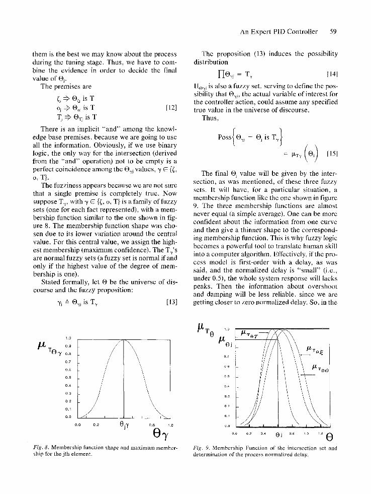
The fuzziness appears because we are not sure that a single premise is completely true. Now suppose Tv, with ~ ~ {~, o, T} is a family of fuzzy sets (one for each fact represented), with a membership function similar to the one shown in figure 8. The membership function shape was chosen due to its lower variation around the central value. For this central value, we assign the highest membership (maximum confidence). The T~'s are normal fuzzy sets (a fuzzy set is normal if and only if the highest value of the degree of membership is one).

Stated formally, let ® be the universe of discourse and the fuzzy proposition:

-/j ~ ®~j is Tv [13]

The proposition (13) induces the possibility distribution

1F[o~j = T7 [141

IIe~ j is also a fuzzy set, serving to define the pos- sibil ity that ®~j, the actual variable of interest for the controller action, could assume any specified true value in the universe of discourse.

Thus ,

Poss(®vj = ®J is Tv} = txT~ (®j) [15]

The final ®j value will be given by the intersection, as was mentioned, of these three fuzzy sets. It will have, for a particular situation, a membership function like the one shown in figure 9. The three membership functions are almost never equal (a simple average). One can be more confident about the information from one curve and then give a thinner shape to the corresponding membership function. This is why fuzzy logic becomes a powerful tool to translate human skill into a computer algorithm. Effectively, if the process model is first-order with a delay, as was said, and the normalized delay is "small" (i.e., under 0.5), the whole system response will lacks peaks. Then the information about overshoot and damping will be less reliable, since we are getting closer to zero normalized delay. So, in the

1.0 f

~ 0.9

TO'y o.8 0.7

0.6

0.5

0 .4

0 ,3

0 ,2

0.1

0 .0

o.o o.~ O i T 0.8 ~.o

Fig. 8. Membership function shape and maximum membership for the jth element.

/xT 0 1.o

oJ07 ToT-- 0.6 ~'~Teo

o.o 0.2 o.~ O j o,8 ~.o ~.2 0

Fig. 9. Membership Function of the intersection set and determination of the process normalized delay.


present situation, the membership function as- sociated with the natural period must be made thinner than the ones corresponding to overshoot and damping. Going further in our analysis, we can see that the system is using two measured values to compute overshoot (first valley over first peak), while the damping is computed with three measured values (first valley and first and second peak). Then, we considered a lower possibility of error for the last case and gave a thinner shape to the membership function corresponding to the overshoot.

The final ®j value mentioned earlier is a fuzzy number. Fuzzy numbers [18] are the elements of a real-number fuzzy set satisfying the following conditions simultaneously: 1. the fuzzy set is convex (see [16] for the defi-

nition); and 2. the fuzzy set is normal (introduced before).

Fuzzy numbers, as ordinary numbers, may be used in arithmetical operations (i.e., multiplica- tion, addition, division, subtraction).

Given a fuzzy number X with a membership function P~x and a fuzzy number Y with a membership function ~y, the quotient Z is defined as another fuzzy number X/Y with a membership function given by

~z = Supx/y min ~x,~y [16]

From equations (11) and (16), a value for the normalized gain Kj may be inferred, with Kj being another fuzzy number like ®j with its membership function ~Kj" Notice that the situation is the same if the measure taken from the response observation is Kj instead of Oj.

The membership functions P~Kj and ~oj so computed are a measure of the uncertainty in the process identification. So they will act as a warn- ing if they are under a predefined threshold. If this is the case, the measure is rejected and the loop response is observed again.

5. The Knowledge Base

Whenever non-sequential situations appear, it is a good idea to use an expert system. In our present approach, there are many such situations.

Consider, for instance, creating the peaks when they are not present or keeping the loop response pattern in the boundary of a predefined specifi- cation with the supervisory rules.

Thus, the knowledge base was organized as a production system plus the knowledge represented in the curves as arrays. The production system structure is shown in figure 10. Its mod- ularity, given by separate bodies of rules, de- creases the search time of the agenda-type infer- ence engine used [19].

Programming to manage the man-machine in- terface is also included.

5.1. Master Controller Rules

Master controller rules are responsible for order- ing the activation of each body of rules in turn, monitoring the error pattern. Although an option for another algorithmic procedure is also possible in this section, we have selected the same expert system shell we use to embody the knowledge, for programming simplicity. An example of this kind of rule may be seen in table 1. This particular rule is fired whenever the peaks in the time response of the entire loop are detected. In this way, the error is being monitored on-line.

5.2. Identification Rules

When the controller is automatically put in identification mode, a variable time sequence is fired. At first, the two tuning presets as described in section 3.1. are generated, computing 6) and K.

MASTER CONTROLLER RULES

CURVE

CONSULTATIVE

REFINED ZIEGLER & NICHOLS

BETA

ADJUSTMENT

IDENTIFICATION RULE, ~

SUPERVISORY

CONTROL

RULES

Fig. IO. Knowledge-base architecture.


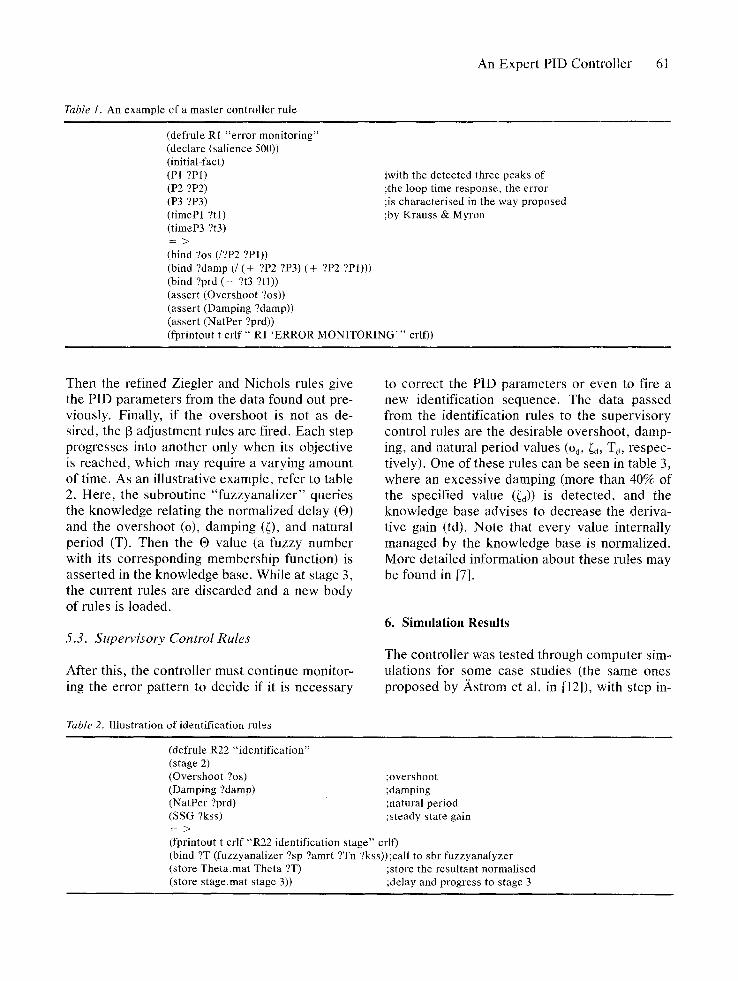
Table 1. An example of a master controller rule

(defrule R1 "error monitoring" (declare (salience 500)) (initial-fact) (P1 ?P1) (P2 ?P2) (P3 ?P3) (timePl ?tl) (timeP3 ?t3) = >

(bind ?os (/?P2 ?P1)) (bind ?damp ( / (+ ?P2 ?P3) (+ ?P2 ?P1))) (bind ?prd ( - ?t3 ?tl)) (assert (Overshoot ?os)) (assert (Damping ?damp)) (assert (NatPer ?prd)) (fprintout t crlf " RI 'ERROR MONITORING'" crlf))

~with the detected three peaks of ;,the loop time response, the error ;is characterised in the way proposed ;by Krauss & Myron

Then the refined Ziegler and Nichols rules give the PID parameters from the data found out previously. Finally, if the overshoot is not as desired, the [3 adjustment rules are fired. Each step progresses into another only when its objective is reached, which may require a varying amount of time. As an illustrative example, refer to table 2. Here, the subroutine "fuzzyanalizer" queries the knowledge relating the normalized delay (®) and the overshoot (o), damping (~), and natural period (T). Then the ® value (a fuzzy number with its corresponding membership function) is asserted in the knowledge base. While at stage 3, the current rules are discarded and a new body of rules is loaded.

5.3. Supervisory Control Rules

After this, the controller must continue monitoring the error pattern to decide if it is necessary

Table 2. Illustration of identification rules

to correct the PID parameters or even to fire a new identification sequence. The data passed from the identification rules to the supervisory control rules are the desirable overshoot, damping, and natural period values (o~, ~d, Td, respectively). One of these rules can be seen in table 3, where an excessive damping (more than 40% of the specified value (~d)) is detected, and the knowledge base advises to decrease the derivative gain (td). Note that every value internally managed by the knowledge base is normalized. More detailed information about these rules may be found in [7].

6. Simulation Results

The controller was tested through computer simulations for some case studies (the same ones proposed by )kstrom et al. in [12]), with step in-

(defrule R22 "identification" (stage 2) (Overshoot ?os) ;overshoot (Damping ?damp) ;damping (NatPer ?prd) ;natural period (SSG ?kss) ;steady state gain = >

(fprintout t crlf "R22 identification stage" crlf) (bind ?T (fuzzyanalizer ?sp ?amrt ?Tn ?kss));call to sbr fuzzyanalyzer (store Theta.mat Theta ?T) ;store the resultant normalised (store stage.mat stage 3)) ;delay and progress to stage 3


Table 3. Example of excessive damping management rule

(defrule R16 "excessive damping" (declare (salience 10)) (Damping ?damp) (DAMESP ?damesp) ?fl < - ( t d ?td) (test (> = ?damp (+ ?damesp 0.4155)))

(fprintout t "R16 excessive damping (s. m.)" crlf) (bind ?td (* ?td 0.8)) (retract ?fl) (assert (td ?td)) (fprintout t "TRYING TO REDUCE THE DAMPING"

crlf) (store td.mat td ?td))

puts of the form shown in figure 11, superim- posed onto the usual loop reference.

The amplitude of these tuning presets should be such that they could be negligible compared to the amplitudes of the set point changes in a normal loop operation. With regard to the period, it was chosen such that the system response can reach its steady state before a new step is in- jec ted into the reference.

This strategy may be compared with a state machine for which groups of steps belong to each state of the controller. So steps 1 and 2 usually correspond to stages described in section 3.1; step 3 corresponds to a refined Ziegler and Ni- chols rules response; and the next two or three steps correspond to a [3 adjustment to obtain a desirable overshoot .

After these set point changes, the controller is tuned. Then it is expected that the loop response to a load change is like the one corresponding to

STEPS 1.oo

AMPLITUDE

O.75

O.5O

0 .26

O ; i s AmDIItud

0,00

o

I I I I I _ _

50 100 160 2 0 0 260

nT

Fig. 11. Input steps.

the third set point variation (refined Ziegler and Nichols type). In the same way, the loop response to a set point change is the one corresponding to the last set point variation of the whole identification stage. This is shown in the following figures.

The processes analyzed were the following:

Process 1 Process 1 corresponds to equation (1), with different delays and time constants, to test the controller in the zones proposed in [12] of "large normalized process gain or small normalized dead-time (2.25 < K < 15; 0.16 < ® < 0.57) and small normalized process gain or large normalized dead-time (1.5 < K < 2.25; 0.57 < ® < 0.96)." The results for each zone are shown in figures 12 and 13, respectively. For figure 12 we simulated process 1 with -r = 0.64 sec., a = 2, and k = l . For figure 13, ¢=2 .5 sec., a=2 .5 , and k = l .

The general procedure for bet ter understand- ing these figures and the ones below is as fol- lows: 1. The first one or two steps are to obtain the

normalized delay (O) and gain (K), and the steady-state gain (kss).

2. The next step is to obtain the ultimate period (tu).

3. The next step is a refined Ziegler and Nichols response.

4. The final steps (up to the last in the figures) are used to tune the set point filter in order to reach the overshoot specifications ([3). It is interesting to see that even in zones of

very small ®, not described explicitly in [12], the performance was good. In this case, process 1 was tested with ~r = 0.5 sec., a = 4, and k = 1. The reason for the slower identification is that for very small ®, the error pattern lacks peaks. Re- member that the plant is put in closed loop with a unitary normalized step reference; then the information about ~, o, and T is more imprecise. The results are shown in figure 14.

A normal loop operation after a prereset for this process with ~- = 0.64 sec., a = 2, and k = 1 is shown in figure 15, where it is compared to a standard Ziegler and Nichols loop response.

--•" 0.4 fk

~ 0.2

1.2 J

0.8

I

O.6 .H~Hnnn

.0.2 1 4, , J

-0.4 ~ ,[i

"0"60 50 100 150 200 250

nT

Fig. 12. Tuning r e s p o n s e for P r o c e s s 1 wi th 0 = 0.32.

1.5

0

-0

n T

Fig. 13, Tuning r e s p o n s e fo r P roce s s 1 wi th 0 = 1,


1.6 r

1,4

1,2

- i I-

0.8

"~l 0.6

i ~ ~ 0.4

-0.20 510 100 1 0 2 250 300 350 400

~T

Fig, 14. Tuning r e s p o n s e for P r o c e s s 1 wi th 0 = 0.125.

Process 2 Equation (17) represents a process family similar to the one represented by equation (1), but with a double co inc iden t cons t an t t ime:

e-SX,: GP(s~ - (1 + s × a) 2 [17]

16

- ] 4

12

5 5

'i L

20 40 60 80 10(3 120

NORMAL1SED TIME

Fig. 15. A c o m p a r i s o n b e t w e e n a re f ined Ziegler and Ni- cho ls r e s p o n s e as i m p l e m e n t e d in this ar t icle ( ) and the s t anda rd Ziegler and Nicho l s r e s p o n s e ( . . . . . . . ) for P r o c e s s 1 wi th 0 = 0.32.


The entire loop behavior for an instance with "r = 1 sec. and a = 1 can be seen in figure 16.

Process 3 Equat ion (18) represents a mult icapaci ty process. The simulation presented in this article is for a = 1 and n = 4. In this way, we verified the assumpt ion made about the simplification proposed in [2].

1 G p ~ ) - (1 + s x a) n [18]

The entire loop behavior may be seen in figure 17.

Process 4 Equat ion (19) is, in some sense, a hard test for the implemented controller because these plants have an inverse dynamical response. This is the reason for the " - s x & ' in the numerator . How- ever, for ~ = 0 . 5 , the loop behavior was highly satisfactory, as can be seen in figure 18.

(1 - s x ~ ) G p ~ , ) - (1 + s) 3 [19]

50 100 150 200 250 360

nT

Fig. 17. Tuning response for Process 3.

350

-02 i

;o 1~o lb 200 ~o 3oo 3~o nT


4OO

d U

50 "t00 150 200 250 300

nT



From the considered cases, evidently the implemented controller works correctly in different situations. The imposed constraints were a refined Ziegler and Nichols load change response, an overshoot lower than or equal to 10%, and limited oscillations. In the simulations, these limits were chosen over 60% undershoot and under 60% overshoot. The limits can be changed from case to case.

An outstanding result is that although one may expect an exact refined Ziegler and Nichols set- ting of the PID parameters, they will belong to a neighborhood. The neighborhood size will be a function of the error pattern parameters measure done. In other words, it will depend on the measure confidence (tXrr). For the cases studied, Ixa- was made larger than 0.7.

7. Conclusions

The experimental results show that it is not only possible but also very useful for typical applications to link the pattern characterization of the process response (in terms o, ~, and T) to the process characterization from the normalized gain and dead-time (K and ®). This approach allows us to apply some well-known heuristics. Of course, this analysis is not exhaustive in every possible case, but for models the analysis ap- proximates a great many industrial processes closely enough. However, studies concerning the limits of applicability should be done.

The other important fact that becomes evi- dent from the results is that the combination of fuzzy logic, PID control, and pattern recognition proved to match acceptably well in control prob- lems where there is a poor or varying plant model. Fuzzy logic contributes to the management of imprecision and missing data. PID control shows again its versatility and drive simplicity. Pattern recognition of the response gives a fast way to on-line evaluation of the overall system performance in a simple manner.

Although our present approach can be seen as "ad-hoc" in some sense, we are just trying to embody empirical knowledge about a particular application. Expert systems and fuzzy logic suit well in these situations.

Further improvements to the control policy can be made, adding some learning capabilities to improve the adaptive behavior. This result can be achieved, for instance, via a neural network [19]. The learning results so acquired may be translated into fuzzy rules.

Another interesting alternative may be the utilization of a model bank with stored time re- sponses. The controller may compare the actual plant response with the ones in the bank. If it gets a similar response, it can consider itself to be in the neighborhood of a model in the bank. Then, fuzzifying this plant model, one can obtain an on- line variable model for the process under control. This, of course, may lead to the prediction of a control action.

Acknowledgments

The authors are members of Laboratorio de Electr6nica Industrial, Control e Instrumenta- ci6n (LEICI), Dto. de Electrotecnia, Fac. de Ingenierfa, Universidad Nacional de La Plata, Argentina, where this work was completely developed, e-mail:leici @ fisflp.edu.ar.

References

1. J.G. Ziegler and N.B. Nichols, "Optimum settings for automatic controllers," Trans. ASME, vol. 65, pp. 433- 444, 1942.

2. F.G. Shinskey, Process-Control Systems, McGraw- Hill: New York, p. 37, 1975.

3. K.J .A.strom and T. Hagglund, "Automatic tuning of simple regulators with specifications on phase and amplitude margins," Automatica, vol. 20, no. 5, pp. 645- 651, 1984.

4. C.C. Hang, T.H. Lee, and T.T. Tay, "The use of recur- sive parameter estimation as an auto-tuning aid," in Proc. 1SA Annu. Conf., USA, 1984, pp. 387-396.

5. C.C. Hang, K.K. Sin, "On-line auto-tuning of PID controllers based on cross correlation," Proc. Int. Conf. Ind. Electron., Singapore, 1988, pp. 441-446.

6. K.J. Astrom, J.J. Anton, and K.E. Arzen, "Exper t control ," Automatica, vol. 22, pp. 277-286, 1986.

7. G.G. Acosta, M.A. Mayosky, and J.M. Catalfo, "Sis- tema de Producci6n aplicado a ta sintonfa de un Con- trolador PID," in Proc. XI I I Jornadas de Ingenier[a El~ctrica y Electrdnica, Quito, Ecuador, July 1992, pp. 657-664.

8. E.H. Bristol, "Pat tern recognition: an alternative to parameter identification in adaptive control ," Auto- matica, vol. 13, no. 2, pp. 197-202, 1977.


9. T.W. Krauss and T.J. Myron, "Self-tuning PID controller uses pat tern recognition approach," Control Eng., vol. 36, no. 6, pp. 106-111, June 1984.

10. R.J. Mantz and E.J. Tacconi, "Complimentary rules to Ziegler and Nichols ' rules for a regulating and tracking controller," Int. J. Control, vol. 49, no. 5, pp. 1465- 1471, 1989.

11. R.J. Mantz and E.J. Tacconi, "A regulating and tracking PID controller," Ind. Eng. Chem. Res., vol. 29, pp. 1249-1253, 1990.

12. C.C. Hang, K.J. Astrom, W.K. Ho, "Refinements of the Ziegler and Nichols tuning formula," lEE Proc. D, vol. 138, no. 2, pp. 111-118, March 1991.

13. P.J. King and E.H. Mamdani, "The application of fuzzy control systems to industrial processes," Auto- matica, vol. 13, pp. 235-242, 1977.

14. F. van der Rhee, H.R. van Nauta Lemke, and J.G. Dijkman, "Knowledge based fuzzy control of sys-

tems," IEEE Trans. Automat. Control, vol. 35, no. 2, pp. 148-155, February 1990.

15. S. Tzafestas and N.P. Papanikolopoulos, "Incremental fuzzy expert PID control ," IEEE Trans. Ind. Electron., vol. 37, no. 5, pp. 365-371, October 1990.

16. L.A. Zadeh, °'Fuzzy sets ," Inform. Control, vol. 8, pp. 338-353, 1965.

17. L.A. Zadeh, "Fuzzy logic," IEEE Computer, pp. 83- 93, April 1988.

18. A. Kaufmann and M.M. Gupta, Introduction to Fuzzy Arithmetic: Theory and Applications, Van Nostrand Reinhold: New York, 1985.

19. E. Rich, Artificial Intelligence, McGraw-Hill: New York, pp. 84-87, 1983 (series in Artificial Intelligence).

20. Dote Yashuiko, "Fuzzy and neural network controller," in Proc. XVI Annu. Conf. IEEE Ind. Electron. Soc. (IECON '90), Asilomar, USA, November 1990, pp. 1314-1324.

Gerardo Gabriel Acosta received the Electronic Engineer- ing degree from the University of La Plata (UNLP, Argen- tina) in 1988. He was a fellow of the CICpBA and a teaching assistant at UNLP from 1988 to 1992. Now he is working toward the Ph.D., sponsored by the Argentinian Research Council (CONICET) in the Faculty of Science at the Uni- versity of Valladolid (Spain). His main research interests are expert and fuzzy systems in real-time control and system supervision.

Miguel Angel Mayosky obtained his Electronic Engineering degree at the University of La Plata (UNLP, Argentina) in 1983, and a Ph.D. in computer architecture at Autonomous University of Barcelona (Spain) in 1990. During 1992 he joined the European Organization for Nuclear Research (CERN) in Geneva, Switzerland, as a Scientific Associate. He is now Professor of Automatic Control at UNLP, and his research work is supported by CICpBA. His main research topics include neural networks and fuzzy systems for control and computer architectures for real-time pro- cessing.

Jos6 Maria Catalfo graduated in Electronic Engineering from the University of La Plata (UNLP, Argentina) in 1969. He then worked in the field of industrial control systems as a research engineer. During 1981/1982 and 1991/1992, he joined the European Organization for Nuclear Research (CERN) in Geneva, Switzerland, as a Scientific Associate. He is now a member of the Argentinian Research Council (CONICET) and Professor of Automatic and Process Con- trol in the Faculty of Engineering at the UNLP. His research area is fuzzy control.

An expert PID controller uses refined ziegler and nichols rules and fuzzy logic ideas

Documents

Transcript of An expert PID controller uses refined ziegler and nichols rules and fuzzy logic ideas