Available online at www.sciencedirect.com

www.elsevier.com/locate/jprocont

Journal of Process Control 18 (2008) 19–26

A novel approach for H2=H1 robust PID synthesisfor uncertain systems

Eduardo N. Goncalves a, Reinaldo M. Palhares b,*, Ricardo H.C. Takahashi c

a Department of Electrical Engineering, Federal Center of Technological Education of Minas Gerais, Av. Amazonas 7675,

31510-470 Belo Horizonte, MG, Brazilb Department of Electronics Engineering, Federal University of Minas Gerais, Av. Antonio Carlos 6627, 31270-010 Belo Horizonte, MG, Brazil

c Department of Mathematics, Federal University of Minas Gerais, Av. Antonio Carlos 6627, 31270-010 Belo Horizonte, MG, Brazil

Received 3 April 2007; received in revised form 27 June 2007; accepted 27 June 2007

Abstract

This paper presents a procedure for robust two-degrees-of-freedom PID synthesis based on a non-convex optimization problem con-sidering the H2 and/or H1 guaranteed costs of the closed-loop transfer matrix as objective functions and constraints together withrobust regional pole placement. The uncertain system can be represented by multiple, polytopic or affine parameter-dependent models.The efficiency of the proposed synthesis procedure is illustrated by examples.� 2007 Elsevier Ltd. All rights reserved.

Keywords: PID controller; Uncertain systems; Robust control

1. Introduction

The proportional-integral-derivative (PID) controllersstill represent, nowadays, the most applied controller con-figuration in industry. More than 90% of all control loopsare PID, with a wide range of applications: process control,motor drives, magnetic and optical memories, automotive,flight control, instrumentation, etc. [1]. This predominanceof PID control is probably due to its simplicity (only threeparameters to adjust), to its effectiveness for the majority ofthe industrial plants, and to the existence of a simple tuningmethod developed by John G. Ziegler and Nathaniel B.Nichols in 1942. In the Ziegler–Nichols step responsemethod, the PID parameters are computed from simplefeatures of the step response. However, it is known thatsuch procedure leads to poor results in many cases [1].Since 1942, several published works have tried to meetthe need for specific synthesis procedures according to

0959-1524/$ - see front matter � 2007 Elsevier Ltd. All rights reserved.

doi:10.1016/j.jprocont.2007.06.003

* Corresponding author. Tel.: +55 31 3409 3457; fax: +55 31 3499 4850.E-mail address: palhares@cpdee.ufmg.br (R.M. Palhares).

the application (auto-tuning, model predictive control,etc) considering quite different objectives and tuning algo-rithm complexity (see the references in [1]). The work [2]presents an overview of PID control and different tuningmethods. The Ziegler–Nichols step response method isrevisited and new tuning rules are developed in [3,4]. Thedesign of PID controllers based on constrained optimiza-tion is developed in [5], where the objective is to maximizethe integral gain subject to constraints over the Nyquistcurve. In [6], a PID tuning procedure is presented basedon the fitting of the process frequency response to a partic-ular second-order plus dead time structure. In [7], a PIDtuning method is presented, based on frequency loop-shap-ing, considering the minimization of the difference betweenthe actual and a target loop transfer function, in an L1sense. The work [8] presents a single PID tuning rule fora first-order or second-order time delay model, and devel-ops simple analytic rules for model reduction to obtain amodel in these forms.

Despite the several PID tuning techniques available forthe different PID configurations and applications (refer to[9] for a extensive list), it is still interesting to research

1 Instrument Society of America.

20 E.N. Goncalves et al. / Journal of Process Control 18 (2008) 19–26

new approaches that can lead to better performance andthat can be applied to a broader class of problems, in spe-cial, the multiobjective robust synthesis to tackle uncertainsystems represented by polytopic, or affine parameter-dependent models. The development of H2=H1 guaran-teed cost characterizations in terms of linear matrixinequalities (LMIs) could be an alternative to developPID tuning approaches for uncertain systems. Unfortu-nately, the PID controller is a structured reduced-orderdynamic output-feedback controller and, to the best ofthe authors’ knowledge, there is no LMI-based formula-tion to tackle this problem: characterizing the problem asa static output-feedback control leads to bilinear matrixinequalities (BMIs) that are non-convex optimizationproblems. In [10], the PID tuning is characterized as arobust multiobjective static output-feedback control prob-lem with an augmented state equation, and LMI-based for-mulations are applied to assess the resulting guaranteedcosts. In [11], the Kharitonov theorem for interval plantsis exploited for the purpose of characterizing all PID con-trollers that stabilize an uncertain plant. In [12], an inte-grated system identification and robust PID tuningstrategy is presented, based on frequency loop-shaping,considering the minimization of the difference betweenthe actual and a target loop transfer function, in anL2=L1 sense. In [13], a robust PID controller designmethod for multiple-models is developed via the LQR-LMI static output-feedback control approach.

This paper presents a two-step robust PID tuning proce-dure based on a non-convex multiobjective optimizationphase and on an LMI-based analysis phase that can beapplied to uncertain linear time-invariant systems repre-sented by multiple, polytopic or affine parameter-depen-dent models. In the optimization phase, a non-convexoptimization problem is solved to compute the PID param-eters, considering a finite set of points of the uncertaintydomain. In the analysis phase, a branch-and-bound algo-rithm that employs LMI-based sufficient conditions asupper bound functions is applied to verify the objectivefunction and constraints for all uncertainty domain. Ifany constraint is violated or there is the possibility toimprove the objective function, new points can be includedin the finite set for a new iteration of the iterative synthesisprocedure. The motivation to consider this procedure is itsprevious successfully applications for robust state-feedbackcontroller synthesis [14], robust static or dynamic output-feedback controller synthesis [15], and filter synthesis [16].Despite the difficulty to tackle non-convex optimizationproblems with only three decision variables (the PIDparameters), it will be illustrated by examples that the pro-posed robust PID tuning procedure can provide better per-formance than previous published approaches consideredhere. Preliminary results have been published in an earlierconference work [17].

In this paper, capital letters are used to indicate theLaplace transform of a signal, e.g., H(s) is the Laplacetransform of g(t).

2. Problem statement

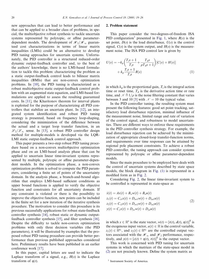
This paper consider the two-degrees-of-freedom ISAPID configuration1 presented in Fig. 1, where R(s) is theset point, D(s) is the load disturbance, U(s) is the controlsignal, C(s) is the system output, and H(s) is the measure-ment noise. The ISA PID control law is given by

UðsÞ ¼ �kp

T isþ 1

T isþ T ds

qT dsþ 1

� �½CðsÞ þ HðsÞ�

þ kp

T isþ 1

T isRðsÞ ð1Þ

in which kp is the proportional gain, Ti is the integral actiontime or reset time, Td is the derivative action time or ratetime, and N,1=q is the noise filtering constant that variesbetween 3 and 10 [3] with N ¼ 10 the typical value.

In the PID controller tuning, the resulting system mustpresent the following features: good set point tracking, sat-isfactory load disturbance rejection, minimal influence ofthe measurement noise, limited range and rate of variationof the control signal, and robustness to model uncertain-ties. There are different ways to enforce these requirementsin the PID controller synthesis strategy. For example, theload disturbance rejection can be achieved by the minimi-zation of appropriate closed-loop transfer-function norms,and requirements over time responses can be attained byregional pole placement constraints. To achieve a robustPID controller, the tuning approach can consider systemsrepresented by polytopic or affine parameter-dependentmodels.

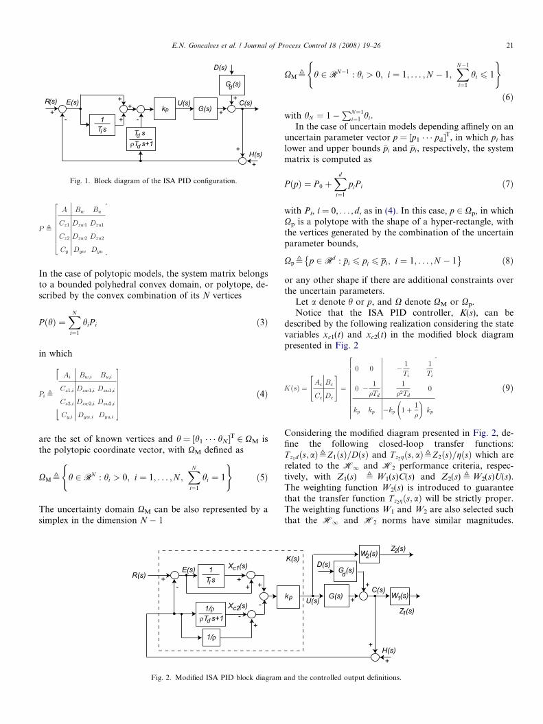
Since the main procedure to be employed here deals withthe control of uncertain systems described by state spacemodels, the block diagram in Fig. (1) is represented in amodified form as in Fig. 2.

Considering Fig. 2, the linear time-invariant system tobe controlled is represented in state-space as

_xðtÞ ¼ AxðtÞ þ BwwðtÞ þ BuuðtÞz1ðtÞ ¼ Cz1xðtÞ þ Dzw1wðtÞ þ Dzu1uðtÞz2ðtÞ ¼ Cz2xðtÞ þ Dzw2wðtÞ þ Dzu2uðtÞyðtÞ ¼ CyxðtÞ þ DywwðtÞ þ DyuuðtÞ

ð2Þ

in which x 2 Rn is the state vector, w(t) = [r(t), d(t), g(t)]T isthe exogenous input vector, uðtÞ 2 R is the control variable,z1ðtÞ 2 Rq1 , and z2ðtÞ 2 Rq2 are the controlled output vec-tors associated with the H1 and H2 performance, respec-tively, and y(t) = [c(t) + g(t), r(t)]T is the output vector.

This work is concerned with PID tuning for uncertainsystems in which the matrices of the state-space model in(2) are not precisely known. Define the system matrix as

G(s)k

T sT s

R(s) U(s)E(s)

H(s)

C(s)

i

p

d

1

T s+1d

D(s)

+

+

+

+

++

+

+

- -

G (s)d

Fig. 1. Block diagram of the ISA PID configuration.

E.N. Goncalves et al. / Journal of Process Control 18 (2008) 19–26 21

In the case of polytopic models, the system matrix belongsto a bounded polyhedral convex domain, or polytope, de-scribed by the convex combination of its N vertices

P ðhÞ ¼XN

i¼1

hiP i ð3Þ

in which

ð4Þ

are the set of known vertices and h = [h1 � � � hN]T 2 XM isthe polytopic coordinate vector, with XM defined as

XM, h 2 RN : hi > 0; i ¼ 1; . . . ;N ;XN

i¼1

hi ¼ 1

( )ð5Þ

The uncertainty domain XM can be also represented by asimplex in the dimension N � 1

1/

T sR(s)E(s)

i

1

T s+1d

+++

+-

-X (s)

X (s)

c2

c1

-

+1/

Fig. 2. Modified ISA PID block diagram

XM, h 2 RN�1 : hi > 0; i ¼ 1; . . . ;N � 1;XN�1

i¼1

hi 6 1

( )ð6Þ

with hN ¼ 1�PN¼1

i¼1 hi.In the case of uncertain models depending affinely on an

uncertain parameter vector p = [p1 � � � pd]T, in which pi haslower and upper bounds �pi and �pi, respectively, the systemmatrix is computed as

P ðpÞ ¼ P 0 þXd

i¼1

piP i ð7Þ

with Pi, i = 0, . . . ,d, as in (4). In this case, p 2 Xp, in whichXp is a polytope with the shape of a hyper-rectangle, withthe vertices generated by the combination of the uncertainparameter bounds,

Xp, p 2 Rd : �pi 6 pi 6 pi; i ¼ 1; . . . ;N � 1� �

ð8Þ

or any other shape if there are additional constraints overthe uncertain parameters.

Let a denote h or p, and X denote XM or Xp.Notice that the ISA PID controller, K(s), can be

described by the following realization considering the statevariables xc1(t) and xc2(t) in the modified block diagrampresented in Fig. 2

ð9Þ

Considering the modified diagram presented in Fig. 2, de-fine the following closed-loop transfer functions:T z1dðs; aÞ,Z1ðsÞ=DðsÞ and T z2gðs; aÞ,Z2ðsÞ=gðsÞ which arerelated to the H1 and H2 performance criteria, respec-tively, with Z1(s) , W1(s)C(s) and Z2(s) ,W2(s)U(s).The weighting function W2(s) is introduced to guaranteethat the transfer function T z2gðs; aÞ will be strictly proper.The weighting functions W1 and W2 are also selected suchthat the H1 and H2 norms have similar magnitudes.

kp

K(s)

G(s)U(s)

H(s)

C(s)

D(s)

+

+

+

+

G (s)d

Z (s)2

W (s)1

Z (s)1

W (s)2

and the controlled output definitions.

22 E.N. Goncalves et al. / Journal of Process Control 18 (2008) 19–26

Particularly, W2(s) is designed as a low-pass filter with highcutting frequency.

The closed-loop system dynamic matrix is denoted byAðaÞ. Consider D � C� the desired closed-loop pole place-ment region (half-plane, disk, sector, or the intersection ofthem) with C� denoting the complex left half-plane. Letcw.c. and dw.c. be the worst case of the H1 and H2 normsin the uncertainty domain

cw:c:, maxa2XkT z1dðs; aÞk1 ð10Þ

dw:c:, maxa2XkT z2gðs; aÞk2 ð11Þ

The robust PID tuning problem can be stated as: find thevalues of kp, Ti, and Td that minimize the maximum normvalues cw.c. and dw.c. subject to kp > 0, Ti P 0, Td P 0, andrðAðaÞÞ � D; 8a 2 X. In this expression, r(Æ) denotes thespectrum of the argument matrix. In the sequel, ri(Æ) willdenote the ith eigenvalue in such set.

The regional pole-placement constraint is useful becausethe optimal H1 controllers may lead to slow set pointresponses [10].

3. PID tuning procedure

Let eXi � X be a finite set of points that belong to thepolytope of uncertain parameters, initialized as the set ofpolytope vertices eX0 ¼ mðXÞ, in which m(Æ) denotes the setof vertices of its argument. Consider the ‘‘worst-case’’points in the finite set eXi, given a PID controller K(s)

ecw:c: ¼ maxa2eX i

kT z1dðs; aÞk1

edw:c: ¼ maxa2eX i

kT z2gðs; aÞk2

ð12Þ

Let cg.c. and dg.c. be e-guaranteed costs such as

cw:c: 6 cg:c: 6 ð1þ eÞcw:c: ð13Þdw:c: 6 dg:c: 6 ð1þ eÞdw:c: ð14Þ

and a(1) 2 X and a(2) 2 X be some polytope coordinatessuch as

kT z1dðs; að1ÞÞk1 P ð1� eÞcg:c: ð15ÞkT z2gðs; að2ÞÞk2 P ð1� eÞdg:c: ð16Þ

Define the set of PID controllers with the realization pre-sented in (9)

eC, KðsÞ : kp > 0; T i P 0; T d P 0; q ¼ 0:1

rðAðaÞÞ � D; 8a 2 eXi

( )ð17Þ

The following auxiliary problem is employed in the pro-posed PID tuning procedure:

Auxiliary Problem: Given the scalars k1 > 0, k2 > 0,k1 + k2 = 1, �1 > 0, and �2 > 0, find kp, Ti, and Td to con-struct K*(s), such as

K�ðsÞ ¼ arg minKðsÞ

maxaðk1kT z1dðs; aÞk1 þ k2kT z2gðs; aÞk2Þ

subject to:

a 2 eX i

KðsÞ 2 eCkT z1dðs; aÞk1 6 �1

kT z2gðs; aÞk2 6 �2

8>><>>:This Auxiliary Problem combines two scalarization tech-niques to transform the original multiobjective probleminto a scalar optimization problem: the weighting problemand �-constraint problem. In the weighting problem theobjective is to minimize a weighted sum of the objectivefunctions. In the �-constraint problem it is considered oneobjective function each time with the other objective func-tion treated as a constraint. Different trade-offs can beachieved varying k1 and k2, without the norm constraints(�1 = �2 =1) or, e.g., keeping k1 = 0, k2 = 1, �2 =1, andvarying �1 in a desired range.

The proposed two phase iterative robust PID tuningprocedure, to be presented in the sequel, transforms theproblem of dealing with an infinite number of points ofthe uncertainty domain in a problem that considers onlya finite set of points. At each iteration, in the synthesisphase, the PID parameters are computed by means of anoptimization algorithm that considers the finite set of poly-tope points eXi. In the analysis phase, considering the wholepolytope X, if the maximum value of the objective functionoccurs in a point outside the finite set eX or if any constraintis not attained in a point belonging to the polytope X, thensuch points are included in the finite set and another opti-mization is processed. The procedure ends when all con-straints are attained for all points in the polytope X andthere is no possibility to minimize the objective functionby means of introducing new points of X in the finite seteX i, considering a relative accuracy index �d.

PID tuning procedure:

Step 1. Initialize i 0, eX0 mðXÞ.Step 2. i i + 1, eXi eXi�1.Step 3. Solve the auxiliary problem to compute K*(s) andecw:c: and/or edw:c:

Step 4. If k1 > 0 or �1 <1 then compute cg.c. and a(1) forK*(s).If að1Þ 62 eX i, then if {k1 > 0 and ðcg:c: � ecw:c:Þ=ecw:c: > ed} or cg.c. > �1, then eXi eXi[fað1Þg.

Step 5. If k2 > 0 or �2 <1 then compute dg.c. and a(2) forK*(s).If að2Þ 62 eXi, then if {k2 > 0 and ðdg:c: � edw:c:Þ=edw:c: > ed} or dg.c. > �2, then eXi eXi[fað2Þg.

Step 6. Verify if 9jjrjðAðaðuÞÞÞ 62 D for any a(u) 2 X. If

true, then eXi eXi [ faðuÞg.Step 7. If eXi 6¼ eXi�1, then goto step 2, else stop.

3.1. Optimization phase

The auxiliary scalar optimization problem can be solvedby means of the cone–ellipsoidal algorithm [18]. Consider

E.N. Goncalves et al. / Journal of Process Control 18 (2008) 19–26 23

the ellipsoid in the iteration k described as Ek ¼ fx 2Rd : ðx� xkÞTQ�1

k ðx� xkÞ 6 1g, where xk is the ellipsoidcenter and Qk ¼ QT

k � 0 is the matrix that determines thedirection and the dimension of the ellipsoid axes. Giventhe initial values x0 and Q0, the ellipsoidal algorithm isdescribed by the following recursive equations:

xkþ1 ¼ xk �1

d þ 1Qk ~m

Qkþ1 ¼d2

d2 � 1Qk �

2

d þ 1Qk ~m~mTQk

� � ð18Þ

with

~m ¼ mkffiffiffiffiffiffiffiffiffiffiffiffiffiffiffiffiffimT

k Qkmk

pwhere x 2 Rd is the vector of optimization parameters (inthis case the PID parameters: x ¼ ½ kp 1=T i 1=T d �TÞand mk is the gradient (or sub-gradient) of the most vio-lated constraint of gðxÞ : Rd ! Rs, when xk is not a feasiblesolution, or the gradient (or sub-gradient) of the objectivefunction, f ðxÞ : Rd ! R, when xk is a feasible solution.The finite difference method is applied to compute the gra-dient. The reader can also see [14, Section 3.1] for details ofhow to compute matrix Qk and the gradient mk. The opti-mization algorithm ends when (fmax � fmin)/fmin 6 �, wherefmax and fmin are the minimal and maximal values of theobjective function at the last N� iterations and � is the pre-scribed relative accuracy.

The optimization algorithm requires the choice of theinitial entries of x0 and Q0. The vector x0, with the initialvalues of the PID parameters, can be generated randomlyor one can use the results of a simple PID tuning technique,e.g., the Ziegler–Nichols method. The matrix Q0 defines thesize and orientation of the initial ellipsoid where the opti-mal solution will be searched. The convergence of the algo-rithm depends on the size of the initial ellipsoid and theprescribed relative accuracy. Obviously, there is a trade-off between the computational effort and the level of objec-tive function minimization that defines the best choice ofQ0, N�, and �.

3.2. Analysis phase

The computation of the e-guaranteed costs (cg.c. or dg.c.),maximum value of the closed-loop transfer function norms(cw.c. or dw.c.) for all uncertain domain, and the correspond-ing coordinates (a(1) or a(2)) is performed by means of ananalysis procedure based on the branch-and-bound algo-rithm [19]. The basic strategy of this procedure is to parti-tion the uncertainty domain such as a lower bound and anupper bound functions converge to the global maximumvalue of the norm. This algorithm ends when the differencebetween the bound functions is smaller than the prescribedrelative accuracy e. The maximum value of the H1 (orH2) norm computed in the vertices of the polytope and

its subdivisions is employed by the algorithm as the lowerbound function. The upper bound function is the maxi-mum value of the H1 (or H2) guaranteed cost computedby means of LMI-based formulations: Lemma 1 presentedin [20] in the case of H1 guaranteed cost and combinationof Lemmas 1 and 2 presented in [21] in the case of H2 guar-anteed cost.

A partition technique based on simplicial meshes [22] isapplied for branching the search region. This technique isparticularly interesting because: (i) it can tackle uncertaintydomains not restricted to the hyper-rectangle case; (ii) itleads to an efficient branching sequence (which shrinksthe search region very fast); and (iii) it allows efficientupper bound function evaluations (requiring the minimalnumber of LMI constraints). Besides the fact that theuncertainty domain for a polytopic system is already a sim-plex, the simplex is the polytope with the minimal numberof vertices in a specific space dimension. Lower number ofvertices means lower complexity of the LMI-based analysisformulations (lower number of scalar decision variablesand LMI rows). This partition technique allows the appli-cation of this analysis procedure to both affine parameter-dependent and polytopic models with high efficiency. In thecase of affine parameter-dependent models, the first parti-tion is performed by the Delaunay triangulation thatdecomposes any polytope in a set of simplices.

The same partition strategy is also applied to the regio-nal pole placement analysis procedure. In this case, theanalysis procedure must subdivide any subpolytope whoserobust D-stability is not established until one of the follow-ing conditions is achieved: all subpolytopes are identified asrobustly D-stable by an LMI-based sufficient condition,proving that the uncertain system is robustly D-stable, orit is found at least one vertex of a subpolytope that is notD-stable, proving that the uncertain system is not robustlyD-stable [23]. When the system is not robustly D-stable, theanalysis procedure returns the coordinates a(u) of oneinstance of a not D-stable model T ziwðs; aðuÞÞ such as9i jriðAðaðuÞÞ 62 D. The capability to find an instance of anot D-stable system is due to the fast search space reduc-tion by the elimination of the simplices that are robustlyD-stable.

The reader can access the Matlab Code for the guaran-teed cost computation and the stability analysis at the web-site [24].

4. Illustrative examples

The results presented in the following examples havebeen computed with the software MATLAB� in a com-puter with an 2.8 GHz processor and 1 Gb system RAM.

Example 1. Consider a continuous stirred tank reactorwith a multiple-model description presented in [13] andalso considered in [25]. Considering a stable operationrange, three models are obtained for different operatingpoints

0 1 2 3 4 5 6 7 8 9 100

0.25

0.5

0.75

1

1.25

1.5

Time (s)

Out

put

Proposed (solid)

Toscano, 2005 (dashdot)

Ge et al., 2002 (dashed)

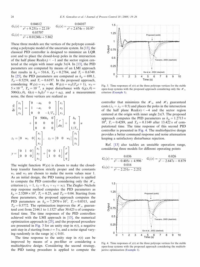
Fig. 3. Time responses of y(t) at the three polytope vertices for the stableopen-loop systems with the proposed approach considering only the H1criterion (Example 1).

0 1 2 3 4 5 6 7 8 9 100

0.25

0.5

0.75

1

1.25

1.5

Time (s)

Out

put

Proposed (solid)

Toscano, 2005 (dashdot)

Ge et al., 2002 (dashed)

Fig. 4. Time responses of y(t) at the three polytope vertices for the stableopen-loop systems with the proposed approach considering the multiob-jective optimization (Example 1).

24 E.N. Goncalves et al. / Journal of Process Control 18 (2008) 19–26

G1ðsÞ ¼0:04612

s2þ 9:251sþ 22:19; G2ðsÞ ¼

0:04107

s2þ 2:674sþ 10:97;

G3ðsÞ ¼0:03707

s2þ 0:01248sþ 5:862

These three models are the vertices of the polytope consid-ering a polytopic model of the uncertain system. In [13], theclassical PID controller is designed to minimize an LQRcost and to place the closed-loop poles in the intersectionof the half plane Real(ri) < �1 and the sector region cen-tered at the origin with inner angle 3p/4. In [13], the PIDparameters are computed by means of an LMI approachthat results in kp = 516.6, Td = 0.2784, and Ti = 0.6749.In [25], the PID parameters are computed as kp = 698.1,Td = 0.5259, and Ti = 0.6197. In the proposed approach,considering W1(s) = w1 = 40, W2(s) = w2/(Tus + 1), w2 =5 · 10�8, Tu = 10�5, a input disturbance with Gd(s,h) =500G(s,h), G(s) = b0/(s2 + a1s + a0), and a measurementnoise, the three vertices are realized as

d

dt

x1

x2

x3

264375 ¼ 0 �a0 0

1 �a1 0

0 0 �1=T u

264375 x1

x2

x3

264375

þ0 500b0 0

0 0 0

0 0 0

264375 r

dg

� �þ

b0

0

1=T u

264375u

z1 ¼ 0 w1 0½ �x1

x2

x3

264375; z2 ¼ 0 0 w2½ �

x1

x2

x3

264375

y ¼0 1 0

0 0 0

� � x1

x2

x3

264375þ 0 0 1

1 0 0

� � r

d

g

264375

The weight function W2(s) is chosen to make the closed-loop transfer function strictly proper and the constantsw1 and w2 are chosen to make the norm values near 1.As an initial design, the PID tuning procedure is appliedto compute the PID controller considering only the H1criterion (k1 = 1, k2 = 0, �1 = �2 =1). The Ziegler–Nicholsstep response method computes the PID parameters askp = 2.5209 · 103, Ti = 0.25, and Td = 0.04. Starting fromthese parameters, the proposed approach computes thePID parameters as kp = 7.2970 · 103, Ti = 0.0315, andTd = 0.5772. The optimization improves the H1 guaran-teed cost from 2144.1 to 1.1527 after 30.625 s of computa-tional time. The time responses of the PID controllersachieved with the LMI approach in [13], the numericaloptimization approach in [25], and the proposed procedureare presented in Fig. 3 for an unity step in r(t), a negativeunit step in d starting from t = 5 s, and a noise signal vary-ing randomly in the range jgj 6 0.01.

The time response to the unity step in r(t) can beimproved by means of a pre-filter or considering amultiobjective design. Considering the second strategy,the PID tuning procedure is applied to compute the

controller that minimizes the H1 and H2 guaranteedcosts (k1 = k2 = 0.5) and places the poles in the intersectionof the half plane Real(r) < �4 and the sector regioncentered at the origin with inner angle 2p/3. The proposedapproach computes the PID parameters as kp = 1.2713 ·104, Ti = 0.4289, and Td = 0.1149 after 13.422 s of com-putational time. The time response of this second PIDcontroller is presented in Fig. 4. The multiobjective designprovides a better command response and noise attenuationkeeping a satisfactory disturbance rejection.

Ref. [13] also tackles an unstable operation range,considering three models for different operating points

G1ðsÞ ¼0:036

s2 � 0:405sþ 4:996; G2ðsÞ ¼

0:026

s2 � 2:647s� 0:879

G3ðsÞ ¼0:016

s2 � 2:251s� 2:252

0 1 2 3 4 5 6 7 8 9 100

0.25

0.5

0.75

1

1.25

1.5

1.75

2

2.25

Time (s)

Out

put

Proposed (solid)

Ge et al., 2000 (dashed)

Fig. 5. Time responses of y(t) at the three polytope vertices for theunstable open-loop systems with the proposed approach considering onlythe H1 criterion (Example 1).

E.N. Goncalves et al. / Journal of Process Control 18 (2008) 19–26 25

The PID parameters kp = 804.6, Ti = 1.3249, andTd = 0.3930 are computed in [13]. Considering only theH1 criterion, the proposed approach computes the PIDparameters as kp = 1.9440 · 104, Ti = 0.0347, and Td =0.4563. The optimization starts from a not robustly stableclosed-loop system to achieve the H1 guaranteed costequal to 0.51742 after 35.687 s of computational time.The time responses of the PID controllers achieved in[13] and the proposed procedure are presented in Fig. 5for the same input considered before. Considering nowthe multiobjective problem, the proposed approach com-putes the PID parameters as kp = 1.3625 · 104, Ti =0.4438, and Td = 0.1285 after 2 iterations (one additionalpoint is included in eX to improve the H2 criterion) and99.734 s of computational time. The time response of thissecond PID controller is presented in Fig. 6.

In this example, in both ranges, the proposed PIDcontrollers computed considering the multiobjective prob-

0 1 2 3 4 5 6 7 8 9 100

0.25

0.5

0.75

1

1.25

1.5

1.75

2

2.25

Time (s)

Out

put Proposed (solid)

Ge et al., 2000 (dashed)

Fig. 6. Time responses of y(t) at the three polytope vertices for theunstable open-loop systems with the proposed approach considering themultiobjective optimization (Example 1).

lem present better tracking responses and disturbancerejections and they are less influenced by the uncertainparameter variations than the PID controllers stated in[13,25].

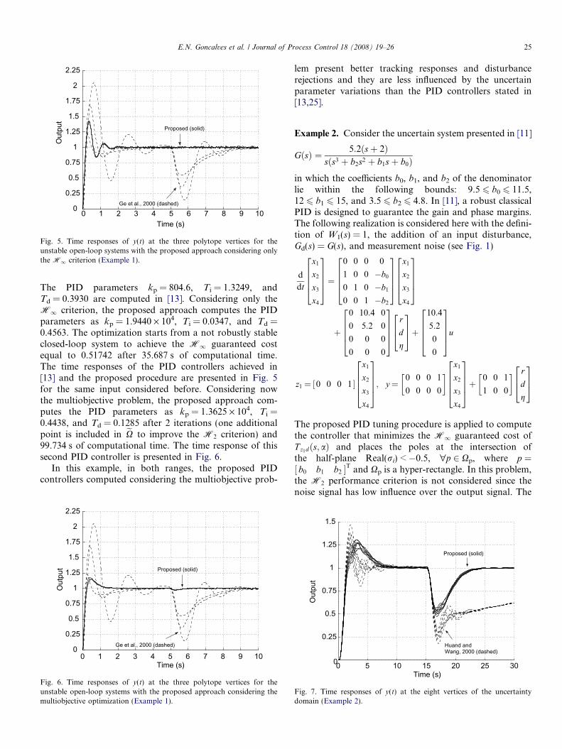
Example 2. Consider the uncertain system presented in [11]

GðsÞ ¼ 5:2ðsþ 2Þsðs3 þ b2s2 þ b1sþ b0Þ

in which the coefficients b0, b1, and b2 of the denominatorlie within the following bounds: 9.5 6 b0 6 11.5,12 6 b1 6 15, and 3.5 6 b2 6 4.8. In [11], a robust classicalPID is designed to guarantee the gain and phase margins.The following realization is considered here with the defini-tion of W1(s) = 1, the addition of an input disturbance,Gd(s) = G(s), and measurement noise (see Fig. 1)

d

dt

x1

x2

x3

x4

2666437775¼

0 0 0 0

1 0 0 �b0

0 1 0 �b1

0 0 1 �b2

2666437775

x1

x2

x3

x4

2666437775

þ

0 10:4 0

0 5:2 0

0 0 0

0 0 0

2666437775

r

d

g

264375þ

10:4

5:2

0

0

2666437775u

z1 ¼ 0 0 0 1½ �

x1

x2

x3

x4

2666437775; y ¼

0 0 0 1

0 0 0 0

� � x1

x2

x3

x4

2666437775þ 0 0 1

1 0 0

� � r

d

g

264375

The proposed PID tuning procedure is applied to computethe controller that minimizes the H1 guaranteed cost ofT z1dðs; aÞ and places the poles at the intersection ofthe half-plane Real(ri) < �0.5, "p 2 Xp, where p ¼½ b0 b1 b2 �T and Xp is a hyper-rectangle. In this problem,the H2 performance criterion is not considered since thenoise signal has low influence over the output signal. The

0 5 10 15 20 25 300

0.25

0.5

0.75

1

1.25

1.5

Time (s)

Out

put

Proposed (solid)

Huand andWang, 2000 (dashed)

Fig. 7. Time responses of y(t) at the eight vertices of the uncertaintydomain (Example 2).

26 E.N. Goncalves et al. / Journal of Process Control 18 (2008) 19–26

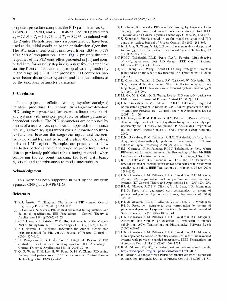
proposed procedure computes the PID parameters as kp =1.6909, Ti = 2.9200, and Td = 0.4629. The PID parameterskp = 3.1950, Ti = 1.3975, and Td = 0.2236, calculated withthe Ziegler–Nichols frequency response method have beenused as the initial condition to the optimization algorithm.The H1 guaranteed cost is improved from 1.834 to 0.777after 58 s of computational time. Fig. 7 presents the timeresponses of the PID controllers presented in [11] and com-puted here, for an unity step in r(t), a negative unit step in d

starting from t = 15 s, and a noise signal varying randomlyin the range jgj 6 0.01. The proposed PID controller pre-sents better disturbance rejection and it is less influencedby the uncertain parameter variations.

5. Conclusion

In this paper, an efficient two-step (synthesis/analysis)iterative procedure for robust two-degrees-of-freedomPID tuning was presented, for uncertain linear time-invari-ant systems with multiple, polytopic or affine parameter-dependent models. The PID parameters are computed bymeans of a non-convex optimization approach to minimizethe H1 and/or H2 guaranteed costs of closed-loop trans-fer-functions between the exogenous inputs and the con-trollable variables, and to robustly place the closed-looppoles at LMI regions. Examples are presented to showthe better performance of the proposed procedure in rela-tion to previously published robust tuning methods, whencomparing the set point tracking, the load disturbancerejection, and the robustness to model uncertainties.

Acknowledgement

This work has been supported in part by the Brazilianagencies CNPq and FAPEMIG.

References

[1] K.J. Astrom, T. Hagglund, The future of PID control, ControlEngineering Practice 9 (2001) 1163–1175.

[2] P. Cominos, N. Munro, PID controllers: recent tuning methods anddesign to specification, IEE Proceedings – Control Theory &Applications 149 (1) (2002) 46–53.

[3] C.C. Hang, K.J. Astrom, W.K. Ho, Refinements of the Ziegler–Nichols tuning formula, IEE Proceedings – D 138 (2) (1991) 111–118.

[4] K.J. Astrom, T. Hagglund, Revisiting the Ziegler Nichols stepresponse method for PID control, Journal of Process Control 14(2004) 635–650.

[5] H. Panagopoulos, K.J. Astrom, T. Hagglund, Design of PIDcontrollers based on constrained optimisation, IEE Proceedings –Control Theory & Applications 149 (1) (2002) 32–40.

[6] Q.-G. Wang, T.-H. Lee, H.-W. Fung, Q. Bi, Y. Zhang, PID tuningfor improved performance, IEEE Transactions on Control SystemsTechnology 7 (4) (1999) 457–465.

[7] E. Grassi, K. Tsakalis, PID controller tuning by frequency loop-shaping: application to diffusion furnace temperature control, IEEETransactions on Control Systems Technology 8 (5) (2000) 842–847.

[8] S. Skogestad, Simple analytic rules for model reduction and PIDcontroller tuning, Journal of Process Control 13 (2003) 291–309.

[9] K.H. Ang, G. Chong, Y. Li, PID control system analysis, design, andtechnology, IEEE Transactions on Control Systems Technology 13(4) (2005) 559–576.

[10] R.H.C. Takahashi, P.L.D. Peres, P.A.V. Ferreira, MultiobjectiveH2=H1 guaranteed cost PID design, IEEE Control SystemsMagazine 17 (5) (1997) 37–47.

[11] Y.J. Huang, Y.-J. Wang, Robust PID tuning strategy for uncertainplants based on the Kharitonov theorem, ISA Transactions 39 (2000)419–431.

[12] E. Grassi, K. Tsakalis, S. Dash, S.V. Gaikwad, W. MacArthur, G.Stei, Integrated identification and PID controller tuning by frequencyloop-shaping, IEEE Transactions on Control Systems Technology 9(2) (2001) 285–294.

[13] M. Ge, M.-S. Chiu, Q.-G. Wang, Robust PID controller design viaLMI approach, Journal of Process Control 12 (2002) 3–13.

[14] E.N. Goncalves, R.M. Palhares, R.H.C. Takahashi, Improvedoptimisation approach to robust H2=H1 control problem for linearsystems, IEE Proceedings – Control Theory & Applications 152 (2)(2005) 171–176.

[15] E.N. Goncalves, R.M. Palhares, R.H.C. Takahashi, Robust H2=H1dynamic output feedback control synthesis for systems with polytopicuncertainty, in: P. Horacek, M. Simandl, P. Zitek (Eds.), Preprints ofthe 16th IFAC World Congress, IFAC, Prague, Czech Republic,2005.

[16] E.N. Goncalves, R.M. Palhares, R.H.C. Takahashi, H2=H1 filterdesign for systems with polytope-bounded uncertainty, IEEE Trans-actions on Signal Processing 54 (9) (2006) 3620–3626.

[17] E.N. Goncalves, R.M. Palhares, R.H.C. Takahashi, H2=H1 robustPID synthesis for uncertain system, in: Proceedings of the 45th IEEEConference on Decision and Control, IEEE, San Diego, USA, 2006.

[18] R.H.C. Takahashi, R.R. Saldanha, W. Dias-Filho, J.A. Ramırez, Anew constrained ellipsoidal algorithm for nonlinear optimization withequality constraints, IEEE Transactions on Magnetics 39 (3) (2003)1289–1292.

[19] E.N. Goncalves, R.M. Palhares, R.H.C. Takahashi, R.C. Mesquita,H2 and H1 e-guaranteed cost computation of uncertain linearsystems, IET Control Theory and Applications 1 (1) (2007) 201–209.

[20] P.J. de Oliveira, R.C.L.F. Oliveira, V.J.S. Leite, V.F. Montagner,P.L.D. Peres, H1 guaranteed cost computation by means ofparameter-dependent Lyapunov functions, Automatica 40 (2004)305–315.

[21] P.J. de Oliveira, R.C.L.F. Oliveira, V.J.S. Leite, V.F. Montagner,P.L.D. Peres, H2 guaranteed cost computation by means ofparameter-dependent Lyapunov functions, International Journal ofSystems Science 35 (5) (2004) 1053–1061.

[22] E.N. Goncalves, R.M. Palhares, R.H.C. Takahashi, R.C. Mesquita,Algorithm 860: SimpleS: an extension of Freudenthal’s simplexsubdivision, ACM Transactions on Mathematical Software 32 (4)(2006) 609–621.

[23] E.N. Goncalves, R.M. Palhares, R.H.C. Takahashi, R.C. Mesquita,New approach to robust D-stability analysis of linear time-invariantsystems with polytope-bounded uncertainty, IEEE Transactions onAutomatic Control 51 (10) (2006) 1709–1714.

[24] R.M. Palhares, H2=H1 guaranteed cost computation – matlab code,http://www.cpdee.ufmg.br/~palhares/software.html, 2007.

[25] R. Toscano, A simple robust PI/PID controller design via numericaloptimization approach, Journal of Process Control 15 (2005) 81–88.