machines

Article

Optimal PID Controllers for AVR System ConsideringExcitation Voltage Limitations Using HybridEquilibrium Optimizer

Martin Calasan 1 , Mihailo Micev 1 , Milovan Radulovic 1, Ahmed F. Zobaa 2,* , Hany M. Hasanien 3

and Shady H. E. Abdel Aleem 4

�����������������

Citation: Calasan, M.; Micev, M.;

Radulovic, M.; Zobaa, A.F.; Hasanien,

H.M.; Abdel Aleem, S.H.E. Optimal

PID Controllers for AVR System

Considering Excitation Voltage

Limitations Using Hybrid

Equilibrium Optimizer. Machines

2021, 9, 265. https://doi.org/

10.3390/machines9110265

Academic Editor: Alejandro

Gómez Yepes

Received: 20 September 2021

Accepted: 28 October 2021

Published: 31 October 2021

Publisher’s Note: MDPI stays neutral

with regard to jurisdictional claims in

published maps and institutional affil-

iations.

Copyright: © 2021 by the authors.

Licensee MDPI, Basel, Switzerland.

This article is an open access article

distributed under the terms and

conditions of the Creative Commons

Attribution (CC BY) license (https://

creativecommons.org/licenses/by/

4.0/).

1 Faculty of Electrical Engineering, University of Montenegro, 81000 Podgorica, Montenegro;martinc@ucg.ac.me (M.C.); mihailom@ucg.ac.me (M.M.); milovanr@ucg.ac.me (M.R.)

2 Electronic and Electrical Engineering Department, Brunel University London, Uxbridge UB8 3PH, UK3 Electrical Power and Machines Department, Faculty of Engineering, Ain Shams University,

Cairo 11517, Egypt; hanyhasanien@ieee.org4 Electrical Engineering Department, Valley Higher Institute of Engineering and Technology, Science Valley

Academy, Qalyubia 44971, Egypt; engyshady@ieee.org* Correspondence: azobaa@ieee.org

Abstract: Automatic voltage regulator (AVR) represents the basic voltage regulator loop in powersystems. The central part of this loop is the regulator, which has parameters that define the speed ofthe voltage regulation, quality of responses, and system stability. Furthermore, it has an impact onthe excitation voltage change and value, especially during transients. In this paper, unlike literatureapproaches, the experimental verifications of the impact of regulator parameters on the excitationvoltage and current value are presented. A novel hybrid metaheuristic algorithm for obtainingregulator parameters determination of the AVR system, and a novel regulator design taking intoaccount excitation voltage limitation are presented. The proposed algorithm combines the propertiesand characteristics of equilibrium optimizer and evaporation rate water cycle algorithms. Theproposed algorithm is effective, fast, and accurate. Both experimental and simulation results showthat the limitation of the excitation voltage increases the settling time of the generator voltage duringreference change. Additionally, the simulation results show that the optimal values of PID parametersare smaller for limited excitation voltage values.

Keywords: automatic voltage regulator; equilibrium–evaporation rate water cycle algorithm; excita-tion voltage; experimental testing; optimization; PID parameters; voltage regulation

1. Introduction

Power systems are dynamic in nature, where their operators must monitor all con-sumers, and regulate energy production of the various energy sources operating and stored.Furthermore, at any moment, the quality of energy, in terms of voltage level and frequency,needs to be in predefined limits [1]. Automatic voltage regulation is an essential controlloop for the generator voltage regulation on the desired value [1–3]. By regulating thegenerator voltage, the voltage in power systems can be efficiently controlled. However,that process depends on the excitation system readiness, and the speed of regulation relieson the regulator parameters. In a mathematical sense, all components of the excitationsystems are nonlinear which indicates that the observation of an automatic regulation loopis not an easy task, particularly with certain assumptions that should be considered [4].

The most important part of the automatic voltage regulator (AVR) is the regulator.Although different variants of regulators can be found in science and practice, the mostcommon regulator is still the proportional-integral-derivative (PID) regulator. Furthermore,different types of PID regulators can be found in the literature—ideal PID [4–17], real

Machines 2021, 9, 265. https://doi.org/10.3390/machines9110265 https://www.mdpi.com/journal/machines

Machines 2021, 9, 265 2 of 28

PID [18–21], fractional-order PID (FOPID) [17,22–30], as well as the higher-order controllers,such as PIDD2 [17,31].

In practice, the majority of tuning methods are based on a process model or onsome non-parametric data from the process. In terms of the controller tuning basedon optimal point search, the research works [4–31] use different algorithms to designthe controller of the AVR system. Some of these works present the usage of improvedkidney-inspired algorithm (IKIA) [4], whale optimization algorithm (WOA) [5], symbioticorganisms search algorithm (SOSA) [6], ant colony optimization (ACO) [8], local unimodalsampling algorithm (LUSA) [9], taguchi combined genetic algorithm (TCGA) [10], simpli-fied particle swarm optimization (SPSO) [11], genetic algorithm (GA) [12], artificial beecolony algorithm (ABCA) [13], chaotic optimization approach (COA) [14], particle swarmoptimization (PSO) [15], equilibrium optimizer algorithm (EOA) [16], hybrid simulatedannealing- manta ray foraging optimization algorithm (SA-MRFA) [17], cuckoo searchalgorithm (CSA) [19,27], teaching-learning based optimization (TLBO) [20], chaotic multi-objective optimization (CMOA) [22,25], artificial bee colony algorithm (ABCA) [23], chaoticant swarm (CAS) [24], multi-objective extremal optimization (MOEO) [26], salp swarmoptimization (SSO) [29], and yellow saddle goatfish algorithm (YSGA) [30] for this purpose.

All the previously mentioned algorithms use different objective functions. The mostcommonly used objective function takes into account different time-domain parame-ters [22–29], such as rise time, settling time, overshoot, and steady state error. However,there are other objective functions in the literature which rely on different frequency-domain parameters [22] such as gain margin, phase margin, gain crossover frequency, andothers. In this regard, the most common objective functions are the integrated absoluteerror (IAE) and integral time absolute error (ITAE) as mentioned in [23,26,29]. Moreover,Zwee Lee Gaing’s function is another common objective function [24,27] that takes intoaccount different time-domain parameters. It is apparent that investigation of the perfor-mance of different optimization algorithms, as well as the objective functions, is popular insolving this engineering problem.

In this paper, a novel hybrid metaheuristic algorithm, called equilibrium optimizer–evaporation rate water cycle algorithm (EO–ERWCA) is presented and tested. The men-tioned hybrid algorithm belongs to the hybrid algorithms that rely on sub-populations.The main idea of the hybridization of this algorithm is to split the population into twosub-populations, and then separately apply the first EO algorithm to one sub-populationand the second ER-WCA algorithm to the other.

Although many research works are dealing with PID parameters design for AVRcontrol, all of them have two significant drawbacks. Firstly, the experimental resultsof the impact of different PID parameters on excitation voltage, excitation current, andgenerator voltage have not been presented in these works. Accordingly, in this paper,experimental validation of the controller performance is presented and analyzed. Secondly,the research works did not take into account the excitation voltage limit. Namely, fieldwinding determines the rated value of the excitation voltage as well as its allowable valueduring transients. Furthermore, the field voltage determines the field current and itsunlimited value can damage the field coils. Therefore, in practice, the field voltage cannotbe unlimited. In practice, the maximum excitation voltage during the “forcing” of theexcitation current (known as ceiling voltage) is in the range between 1.6 p.u (p.u denotesa per-unit value) and 3 p.u [3,32,33]. The ceiling voltages above 2 p.u are difficult torealize because of magnetic saturation [3]. Additionally, in this case, the field current isimpossible to be observed and controlled. Therefore, in a real power system, an excitationvoltage value higher than 3 p.u cannot be realized. This problem is noted in [32,33].In [32], the excitation voltage is limited by limiters, which can be represented by upper andlower limits. The limiters represent the elements for the limitation of the amplitude andspeed of change of certain variables. In the excitation system, the limits are set only forvariables that have a significant impact on the minimum and maximum excitation voltageor current value. Typically, in excitation systems, there are two types of limiters—windup

Machines 2021, 9, 265 3 of 28

and anti-windup. Windup protection is based on setting the output variable (excitationvoltage) to the corresponding minimum/maximum limit value if it exceeds the pre-definedlimits. On the other side, the anti-windup protection, despite considering the value ofthe output variable, also takes into account its speed of change. In other words, the anti-windup changes the states of the controller when there is a difference between unlimitedand limited controller output. A block diagram of the AVR structure with the limiter ispresented in [32]. However, taking into account that the excitation voltage limit is notconcerned in previously published papers dealing with the AVR controller design.

In [33], the excitation voltage limit was taken into account during PID parametersdesign. Furthermore, several comparisons among different PID values in terms of theexcitation voltage value were introduced. However, in both papers, experimental validationof the controller performance was not presented. Additionally, the impact of excitationvoltage/current limitation on the optimal PID parameters design was not analyzed. Theseissues represent the research goal of this work.

The organization of this paper is as follows. Section 2 gives a short overview of thecomposition of the AVR system. A comparison of the literature approaches that deal withthe optimization of different types of PID controllers, with excitation voltage discussion, isgiven in Section 3. A detailed description and mathematical formulation of the proposedEO–ERWCA algorithm are given in Section 4. Section 5 shows the results obtained from thesimulations that are carried out in this paper. The experimental investigation of the impactof the excitation voltage and AVR controller values on the generator voltage response ispresented in Section 6. Finally, conclusions are presented in Section 7.

2. Automatic Voltage Regulation System

The AVR system consists of five components—regulator (R), amplifier (A), exciter(E), generator (G), and sensor (S). The block diagram of an AVR system is illustrated inFigure 1. The regulator uses the signal obtained from the difference between the referenceand measured (sensed) generator voltage and generates a control signal for the amplifierto amplify the signal. In modern excitation systems, it is a microprocessor unit. Themost-used regulator in AVR systems is the PID regulator. The ideal PID regulator is notoften used [4–17] in the literature. Some research works present the usage of real PID (inwhich the derivative action is filtered) [18–21], fractional-order PID regulator (in which thefractional calculus is added to the PID regulator) [22–30], and higher-order controller orPIDD2 [31].

Machines 2021, 9, x FOR PEER REVIEW 3 of 28

that have a significant impact on the minimum and maximum excitation voltage or cur-

rent value. Typically, in excitation systems, there are two types of limiters—windup and

anti-windup. Windup protection is based on setting the output variable (excitation volt-

age) to the corresponding minimum/maximum limit value if it exceeds the pre-defined

limits. On the other side, the anti-windup protection, despite considering the value of the

output variable, also takes into account its speed of change. In other words, the anti-

windup changes the states of the controller when there is a difference between unlimited

and limited controller output. A block diagram of the AVR structure with the limiter is

presented in [32]. However, taking into account that the excitation voltage limit is not

concerned in previously published papers dealing with the AVR controller design.

In [33], the excitation voltage limit was taken into account during PID parameters

design. Furthermore, several comparisons among different PID values in terms of the ex-

citation voltage value were introduced. However, in both papers, experimental validation

of the controller performance was not presented. Additionally, the impact of excitation

voltage/current limitation on the optimal PID parameters design was not analyzed. These

issues represent the research goal of this work.

The organization of this paper is as follows. Section 2 gives a short overview of the

composition of the AVR system. A comparison of the literature approaches that deal with

the optimization of different types of PID controllers, with excitation voltage discussion,

is given in Section 3. A detailed description and mathematical formulation of the proposed

EO–ERWCA algorithm are given in Section 4. Section 5 shows the results obtained from

the simulations that are carried out in this paper. The experimental investigation of the

impact of the excitation voltage and AVR controller values on the generator voltage re-

sponse is presented in Section 6. Finally, conclusions are presented in Section 7.

2. Automatic Voltage Regulation System

The AVR system consists of five components—regulator (R), amplifier (A), exciter

(E), generator (G), and sensor (S). The block diagram of an AVR system is illustrated in

Figure 1. The regulator uses the signal obtained from the difference between the reference

and measured (sensed) generator voltage and generates a control signal for the amplifier

to amplify the signal. In modern excitation systems, it is a microprocessor unit. The most-

used regulator in AVR systems is the PID regulator. The ideal PID regulator is not often

used [4–17] in the literature. Some research works present the usage of real PID (in which

the derivative action is filtered) [18–21], fractional-order PID regulator (in which the frac-

tional calculus is added to the PID regulator) [22–30], and higher-order controller or PIDD2

[31].

Figure 1. Block diagram of the AVR system. Figure 1. Block diagram of the AVR system.

Machines 2021, 9, 265 4 of 28

The ideal PID regulator has three parameters i.e., gains—proportional kp, integral ki,and differential kd. The transfer function of the ideal PID regulator in the s-domain is givenas follows:

PIDideal(s) = kp +kis+ kds (1)

In a real PID controller, the derivative action of the ideal PID controller is filtered withthe filter time constant Tf. Its transfer function is given as follows:

PIDreal = kp +kis+ kd

(s

1 + Tf s

)(2)

The FOPID controller has five parameters kp, ki, kd, µ, and λ, where µ and λ representthe order of the derivative and the integral. The FOPID transfer function is given as follows:

FOPID = kp +ki

sλ+ kdsµ (3)

The PIDD2 controller has also an additional parameter that represents second-orderderivative gain (kd2), in addition to the standard parameters kp, ki, and kd. Its transferfunction is given as follows:

PIDD2 = kp +kis+ kds + kd2s2 (4)

The amplifier is a power element, which increases the power of the control signaland generates a signal of appropriate power for the exciter control. Mathematically, theamplifier can be represented as a first-order transfer function WA with gain kA and timeconstant TA as follows:

WA(s) =kA

1 + sTA(5)

In modern power systems, the exciter represents the power electronic device, usually,it is a thyristor rectifier bridge. This device receives the control signal from the amplifierand defines the excitation voltage value. At present, power electronic devices, such asrectifier bridges, are fast and easy to be controlled. They can be mathematically representedas a first-order transfer function WE with gain kE and time constant TE as follows:

WE(s) =kE

1 + sTE(6)

The most complicated element in the excitation system is the synchronous machine.The most frequently used model of the synchronous generator (SG) is very complicated andit consists of seven differential equations, which are derived from Park’s transformations.However, in the literature, all the components of an AVR loop are formulated as first-ordertransfer functions WG with gain kG and time constant TG as follows:

WG(s) =kG

1 + sTG(7)

The parameters of generator, exciter, amplifier and sensor used are the same in allresearch—kG = 1, TG = 1, kE = 1, TE = 0.4, kA = 10, TA = 0.1.

3. Related Works

In this section, an overview of the existing studies dealing with PID design in AVRsystems is presented. Table 1 presents the optimal values of the parameters for differenttypes of PID controllers (ideal PID, real PID, FOPID, and PIDD2) that are tuned by differentalgorithms. Using the presented data, different simulations were carried out to obtainstep responses of the AVR system. A comparison of the obtained results, in terms of the

Machines 2021, 9, 265 5 of 28

rise time, delay time, overshoot, settling time, and maximum value of excitation voltageis presented in Figures 2–6, respectively. For the presented results, it is clear that all theexisting methods guarantee null steady state error. However, there are big differences interms of the characteristic time metrics (overshoot, rise time, settling time), which meansthat these different methods do not provide the optimal PID design so far.

Machines 2021, 9, x FOR PEER REVIEW 6 of 28

Method

Number Ref.

Regu-

lator kp ki kd Tf μ λ kd2

42

[22]

FOPID

0.408 0.374 0.1773 - 1.3336 0.6827 -

43 0.9632 0.3599 0.2816 - 1.8307 0.5491 -

44 1.0376 0.3657 0.6546 - 1.8716 0.5497 -

45 [23] 1.9605 0.4922 0.2355 - 1.4331 1.5508 -

46 [24]

1.0537 0.4418 0.251 - 1.1122 1.0624 -

47 0.9315 0.4776 0.2536 - 1.0838 1.0275 -

48

[25]

0.9894 1.7628 0.3674 - 0.7051 0.9467 -

49 0.8399 1.3359 0.3511 - 0.7107 0.9146 -

50 0.4667 0.9519 0.2967 - 0.2306 0.8872 -

51 [26] 2.9737 0.9089 0.5383 - 1.3462 1.1446 -

52

[27]

2.5490 0.1759 0.3904 - 1.3800 0.9700 -

53 2.5150 0.1629 0.3888 - 1.3800 0.9700 -

54 2.4676 0.302 0.4230 - 1.3800 0.9700 -

55 [28] 1.5338 0.6523 0.9722 - 1.2090 0.9702 -

56 [29] 1.9982 1.1706 0.5749 - 1.1656 1.1395 -

57 [30] 1.7775 0.9463 0.3525 - 1.2606 1.1273 -

58 [17] 1.8931 0.8699 0.3595 1.2780 1.0408

59 [31] PIDD2

2.7784 1.8521 0.9997 - - - 0.073

60 [17] 2.9943 2.9787 1.5882 - - - 0.102

Figure 2. Rise time of the generator voltage for the different methods presented in Table 1. Figure 2. Rise time of the generator voltage for the different methods presented in Table 1.

Machines 2021, 9, x FOR PEER REVIEW 7 of 28

Figure 3. Delay time of the generator voltage.

Figure 4. Settling time of the generator voltage.

Figure 3. Delay time of the generator voltage.

Machines 2021, 9, 265 6 of 28

Table 1. Summary of the optimal parameters obtained using different controllers/algorithms in the investigated works.

MethodNumber Ref. Regulator kp ki kd Tf µ λ kd2

1 [4]

Ideal PID

1.0426 1.0093 0.5999 - - - -2 [5] 0.7847 0.9961 0.3061 - - - -3 [6] 0.5693 0.4097 0.1750 - - - -4

[7]0.9685 1.0000 0.8983 - - - -

5 0.9519 0.9997 0.8994 - - - -6 0.86832 0.9325 0.9419 - - - -7 [8] 0.6739 0.5951 0.2622 - - - -8 0.6348 0.4801 0.2267 - - - -9

[9]

1.2012 0.9096 0.4593 - - - -10 0.5878 0.4062 0.1843 - - - -11 0.6022 0.3793 0.1841 - - - -12 1.2930 0.9828 0.6303 - - - -13 0.6190 0.4222 0.2058 - - - -14 [10] 0.5600 0.5000 0.2000 - - - -15

[11]

0.5857 0.4189 0.1772 - - - -16 0.9931 0.7461 0.4249 - - - -17 0.9877 0.7780 0.5014 - - - -18 0.9544 0.9434 0.9909 - - - -19

[12]0.6823 0.6138 0.2678 - - - -

20 0.6800 0.5221 0.2440 - - - -21 0.6727 0.4786 0.2298 - - - -22 [13] 1.6524 0.4083 0.3654 - - - -23

[14]

0.6710 0.5050 0.2640 - - - -24 0.6390 0.4770 0.2340 - - - -25 0.6480 0.4780 0.2410 - - - -26 0.6220 0.4530 0.2180 - - - -27 0.6590 0.4870 0.2540 - - - -28

[15]

0.6568 0.5393 0.2458 - - - -29 0.6751 0.5980 0.2630 - - - -30 0.6570 0.5390 0.2458 - - - -31 0.6271 0.4652 0.2209 - - - -32 0.6477 0.5128 0.2375 - - - -33 0.6476 0.5216 0.2375 - - - -34 [16] 0.6829 0.6321 0.2716 - - - -35 [17] 0.6778 0.3802 0.2663 - - - -36

[18]

Real PID

0.6392 0.4757 0.2159 0.0021 - - -37 0.3120 0.2567 0.1503 0.002 - - -38 0.5463 0.3409 0.1485 0.002 - - -39 [19] 0.6198 0.4165 0.2126 0.001 - - -40 [20] 0.5302 0.4001 0.1787 0.0057 - - -41 [21] 0.7080 0.6560 0.2820 0.001 - - -42

[22]

FOPID

0.408 0.374 0.1773 - 1.3336 0.6827 -43 0.9632 0.3599 0.2816 - 1.8307 0.5491 -44 1.0376 0.3657 0.6546 - 1.8716 0.5497 -45 [23] 1.9605 0.4922 0.2355 - 1.4331 1.5508 -46 [24] 1.0537 0.4418 0.251 - 1.1122 1.0624 -47 0.9315 0.4776 0.2536 - 1.0838 1.0275 -48

[25]0.9894 1.7628 0.3674 - 0.7051 0.9467 -

49 0.8399 1.3359 0.3511 - 0.7107 0.9146 -50 0.4667 0.9519 0.2967 - 0.2306 0.8872 -51 [26] 2.9737 0.9089 0.5383 - 1.3462 1.1446 -52

[27]2.5490 0.1759 0.3904 - 1.3800 0.9700 -

53 2.5150 0.1629 0.3888 - 1.3800 0.9700 -54 2.4676 0.302 0.4230 - 1.3800 0.9700 -55 [28] 1.5338 0.6523 0.9722 - 1.2090 0.9702 -56 [29] 1.9982 1.1706 0.5749 - 1.1656 1.1395 -57 [30] 1.7775 0.9463 0.3525 - 1.2606 1.1273 -58 [17] 1.8931 0.8699 0.3595 1.2780 1.040859 [31]

PIDD2 2.7784 1.8521 0.9997 - - - 0.07360 [17] 2.9943 2.9787 1.5882 - - - 0.102

Machines 2021, 9, 265 7 of 28

Machines 2021, 9, x FOR PEER REVIEW 7 of 28

Figure 3. Delay time of the generator voltage.

Figure 4. Settling time of the generator voltage. Figure 4. Settling time of the generator voltage.

Machines 2021, 9, x FOR PEER REVIEW 8 of 28

Figure 5. Overshoot of the generator voltage.

Figure 6. Maximum value of excitation voltage.

These differences can be better viewed on the 3D graphs presented in Figures 7 and

8. These graphs are plotted with a time step of 0.03. Namely, in this figure, the generator

and excitation voltage responses of the AVR system via different PID parameters obtained

using the methods presented in Table 1 are shown.

Figure 5. Overshoot of the generator voltage.

Machines 2021, 9, 265 8 of 28

Machines 2021, 9, x FOR PEER REVIEW 8 of 28

Figure 5. Overshoot of the generator voltage.

Figure 6. Maximum value of excitation voltage.

These differences can be better viewed on the 3D graphs presented in Figures 7 and

8. These graphs are plotted with a time step of 0.03. Namely, in this figure, the generator

and excitation voltage responses of the AVR system via different PID parameters obtained

using the methods presented in Table 1 are shown.

Figure 6. Maximum value of excitation voltage.

These differences can be better viewed on the 3D graphs presented in Figures 7 and 8.These graphs are plotted with a time step of 0.03. Namely, in this figure, the generatorand excitation voltage responses of the AVR system via different PID parameters obtainedusing the methods presented in Table 1 are shown.

Machines 2021, 9, x FOR PEER REVIEW 9 of 28

Figure 7. Generator voltage responses of the AVR system via different PID parameters.

Figure 8. Excitation voltage responses of the AVR system via different PID parameters.

It can be seen that the best system responses were using PIDD2 compared to others.

Additionally, it is more than evident that observing settling time, as well as overshoot are

important time-domain parameters. Regarding the maximum value of the excitation volt-

age calculated via the different methods in Table 1, in all cases, the maximum value of the

excitation voltage is higher than the permitted limit (limit is plotted with the bold line in

Figure 6). For that reason, it can be concluded that the existing PID values do not guaran-

tee a safe operation of the generator even at small voltage pulsations. For that reason,

Figure 7. Generator voltage responses of the AVR system via different PID parameters.

Machines 2021, 9, 265 9 of 28

Machines 2021, 9, x FOR PEER REVIEW 9 of 28

Figure 7. Generator voltage responses of the AVR system via different PID parameters.

Figure 8. Excitation voltage responses of the AVR system via different PID parameters.

It can be seen that the best system responses were using PIDD2 compared to others.

Additionally, it is more than evident that observing settling time, as well as overshoot are

important time-domain parameters. Regarding the maximum value of the excitation volt-

age calculated via the different methods in Table 1, in all cases, the maximum value of the

excitation voltage is higher than the permitted limit (limit is plotted with the bold line in

Figure 6). For that reason, it can be concluded that the existing PID values do not guaran-

tee a safe operation of the generator even at small voltage pulsations. For that reason,

Figure 8. Excitation voltage responses of the AVR system via different PID parameters.

It can be seen that the best system responses were using PIDD2 compared to others.Additionally, it is more than evident that observing settling time, as well as overshootare important time-domain parameters. Regarding the maximum value of the excitationvoltage calculated via the different methods in Table 1, in all cases, the maximum valueof the excitation voltage is higher than the permitted limit (limit is plotted with the boldline in Figure 6). For that reason, it can be concluded that the existing PID values do notguarantee a safe operation of the generator even at small voltage pulsations. For thatreason, special attention to PID design should be paid if the investigated generator wasoperating in a weak network.

4. Equilibrium Optimizer–Evaporation Rate Water Cycle Algorithm

This article proposes a novel hybrid metaheuristic algorithm called equilibriumoptimizer–evaporation rate water cycle (EO–ERWCA) algorithm for determining the opti-mal values of PIDD2 controller parameters. In this regard, hybrid metaheuristic algorithmscan be constructed using different hybridization strategies [34] based on populations, sub-populations, and individuals. The hybrid algorithm proposed in this paper belongs tothe hybrid algorithms based on sub-populations. The main idea is to split the populationinto two sub-populations, and then separately apply the EO algorithm [35] on one sub-population and the ER-WCA algorithm [36] on the other sub-population. These algorithmshave been chosen because of their extremely high efficiency in solving problems relatedto the estimation of the parameters [37,38]. General steps of such a hybrid algorithm aredepicted in the following pseudo-code in Algorithm 1:

Algorithm 1 Hybrid EO-ERWCA Algorithm: Pseudo-Code

Pseudo-code of hybrid EO-ERWCA algorithmRandomly initialize the populationSplit the population into two sub-populationsfor iterator = 1 to max_iterationsfor m = 1 to population_sizeUpdate the first sub-population using the EO algorithmUpdate the second sub-population using ER—WCA algorithmend forend forDetermine the best individual from both sub-populations

Machines 2021, 9, 265 10 of 28

4.1. EO Algorithm

The population consists of a certain number of individuals, denoted with N. In theEO algorithm, each individual is represented with its concentration, which stands for thepotential solution of the optimization problem. Before the iterative procedure starts, thepopulation of the algorithm is randomly initialized between the lower and upper boundsof the optimization variables. The concentration of each particle C at iteration ite is updatedusing Equation (8), and it depends on Ceq—equilibrium concentration, F—exponential term,G—generation rate, λ—turnover rate, V—volume (set to unity in this work), as follows:

C(ite) = Ceq +(C(ite− 1)− Ceq

)F +

GλV

(1− F) (8)

→ The first term Ceq is called equilibrium concentration and it stands for the randomconcentration chosen from the equilibrium pool Ceq,pool. This pool consists of fourbest solutions after each iteration and their average value is formulated as follows:

Ceq,pool ={

Ceq(1), Ceq(2), Ceq(3), Ceq(4), Ceq(ave)

},

Ceq(ave) =Ceq(1)+Ceq(2)+Ceq(3)+Ceq(4)

4 .(9)

→ The second term consists of the difference between the concentration in the previousiteration and the current equilibrium concentration, scaled with exponential term F.This part of Equation (9) forces the global search of the algorithm, or so-called theexploration phase. The exponential term is defined as follows:

F = e−λ(t−t0) (10)

where λ denotes the turnover rate and consists of random numbers in the range [0, 1]. Theexponential term is also defined with vectors t and t0, which are calculated as follows:

t =(

1− itemax_ite

)a2ite

max_ite(11)

t0 =1λ

ln[−a1

(1− e−λt

)· sign(r− 0.5)

]+ t (12)

where max_ite stands for the number of iterations of the algorithm, a1 and a2 are constantswhose values are set to 2 and 1, respectively, while r is a vector of random numbers in therange [0, 1].

→ The third term focuses on the local search of the algorithm, and is defined with thegeneration rate G, which is calculated using Equation (13):

G = G0e−λ(t−t0) = G0F (13)

The initial value of the generation rate is denoted with G0 and can be determined asfollows:

G0 = GCP(Ceq − λC(ite− 1)

)(14)

where GCP stands for generation rate control parameter, whose value depends on genera-tion probability GP, which is set to 0.5, and random numbers in the range [0, 1], denotedwith r1 and r2.

GCP =

{0.5r1, r2 ≥ GP

0, r2 < GP(15)

Finally, after reaching the selected number of iterations, the optimal solution of theEO algorithm is represented by the concentration of the individual with the lowest fitnessfunction value.

Machines 2021, 9, 265 11 of 28

4.2. ER-WCA Algorithm

The second sub-population is handled by the ER–WCA algorithm. Similar to the EOalgorithm, the sub-population of the total population that belongs to ER–WCA algorithm isalso randomly initialized between boundaries of the optimization variables. The populationof ER–WCA algorithm consists of the sea, rivers, and streams. Precisely, there is one sea,the number of rivers is predefined with the parameter Nr, and the number of streams isdetermined with Ns = Npop − Nr − 1, where Npop stands for the population size. Thisalgorithm is based on the water cycle process that normally occurs in nature. Namely, eachstream in nature flows to the river or the sea. Therefore, the number of streams that belongto each river and the sea must be determined using Equation (16).

NSn = round

∣∣∣∣∣∣∣∣∣

CnNsr∑

n=1Cn

∣∣∣∣∣∣∣∣∣Ns

, n = 1, 2, . . . , Nsr, (Nsr = Nr + 1) (16)

where NSn denotes the number of streams that flow into the nth river or the sea if n equals 1is assumed. In the previous equation, round{} stands for the rounding to the nearest integernumber, while || denotes the absolute value. Additionally, Cn is calculated as follows:

Cn = f (Xn)− f (XNsr+1), n = 1, 2, . . . , Nsr (17)

where Xi represents the ith individual of the population, and f () stands for the fitnessfunction. Each stream can flow to either river or sea. The mathematical formulations willdiffer depending on the final destination of the stream. If the stream flows into the river, itsposition that is denoted Xstream is updated using Equation (18). Thus:

Xstream(ite) = Xstream(ite− 1) + rand · C(Xriver(ite− 1)− Xstream(ite− 1)) (18)

The other possible situation is that the stream flows into the sea. In this case, theposition of the corresponding stream is updated using Equation (19):

Xstream(ite) = Xstream(ite− 1) + rand · C(Xsea(ite− 1)− Xstream(ite− 1)) (19)

In the previous equations, rand stands for a random number between 0 and 1 that isgenerated separately for each stream, while C is a predefined parameter that is selected tobe 2, according to [36].

After the update procedure for each stream is finished, it is necessary to compare thefitness functions of such obtained streams and the corresponding river. If a certain streamhas a lower value of the fitness function than the river, that stream becomes the river, andvice versa (their roles are switched).

A similar procedure is also carried out for the rivers. Namely, the position of eachriver is updated using Equation (20).

Xriver(t) = Xriver(t) + rand · C(Xsea(t)− Xriver(t)) (20)

The fitness function of updated rivers must be calculated and compared with thefitness function of the sea. If a river has a lower fitness function value than the sea, theirpositions will be swapped.

The final stage of ER–WCA is the process of evaporation. The evaporation can occurin two cases:

→ Firstly, if the river has only a few streams, it can evaporate even before it reaches thesea. The chance of evaporation is defined with the evaporation rate (ER):

ER =sum(NSn)

Nsr − 1· rand, n = 2, 3, . . . , Nsr (21)

Machines 2021, 9, 265 12 of 28

If the evaporation occurs, the river disappears but the new stream is formed from thevapor, so that:

Xnewstream = LB + rand · (UB− LB) (22)

where LB and UB stand for the lower and upper bounds of optimization variables, respec-tively.

In summary, the evaporation process of the rivers can be summarized as follows:

if(

e−ite

max_ite < rand)

&(NSi < ER), i = 1, 2, . . . , Nr

Xnewstream = LB + rand · (UB− LB);

end if

(23)

→ Secondly, rivers and streams can flow to the sea. Afterward, the seawater willevaporate. The evaporation in the case when river flows into the sea is modeledas follows:

if(|Xsea − Xi| < dmax)or(rand < 0.1), i = 1, 2, . . . , NrXnew

stream = LB + rand · (UB− LB);end if

(24)

Similar to this, the evaporation of the seawater when the stream flows into the sea isdescribed with Equation (25):

if(|Xsea − Xi| < dmax), i = 1, 2, . . . , NsXnew

stream = Xsea +√

µ · randn;end if

(25)

where µ is a parameter, whose value is set to 0.1 [36]. Furthermore, randn(1, N) is a vectorof standard Gaussian numbers, and dmax is a parameter that changes at each iteration,as follows:

dmax(ite) = dmax(ite− 1)− dmax(ite)max_ite

(26)

Finally, after the end of the evaporation process, one iteration of the ER–WCA algo-rithm is completed. The described process should be repeated until the maximum numberof iterations is reached. Then, the individual with the lowest fitness function value standsfor the optimal solution of ER–WCA algorithm. The global optimal solution of the problemis obtained by comparing the solution obtained from the first sub-population which ishandled by the EO algorithm and the other solution from the second sub-population thatis handled by the ER–WCA algorithm. The procedure of the hybrid EO–ERWCA algorithmfor determining the optimal set of PIDD2 controller parameters can be summarized by theflowchart presented in Figure 9.

The maximum number of iterations is the parameter that should be carefully chosen.It is important not to set this parameter to be too high because it will slow down theoptimization process, but also it should not be too small because the optimal solution mightnot be reached. In this work, the maximum number of iterations is set to 100.

Machines 2021, 9, 265 13 of 28

Machines 2021, 9, x FOR PEER REVIEW 13 of 28

0.1 , 1,2,...,

;

sea i max r

new

stream

X X d or rand i N

X LB rand UB LB

if

endif

(24)

Similar to this, the evaporation of the seawater when the stream flows into the sea is

described with Equation (25):

, 1,2,...,

;

sea i max s

new

stream sea

X X d i N

X X randn

if

endif

(25)

where μ is a parameter, whose value is set to 0.1 [36]. Furthermore, randn(1, N) is a vector

of standard Gaussian numbers, and dmax is a parameter that changes at each iteration, as

follows:

1_

max

max max

d ited ite d ite

max ite (26)

Finally, after the end of the evaporation process, one iteration of the ER–WCA algo-

rithm is completed. The described process should be repeated until the maximum number

of iterations is reached. Then, the individual with the lowest fitness function value stands

for the optimal solution of ER–WCA algorithm. The global optimal solution of the prob-

lem is obtained by comparing the solution obtained from the first sub-population which

is handled by the EO algorithm and the other solution from the second sub-population

that is handled by the ER–WCA algorithm. The procedure of the hybrid EO–ERWCA al-

gorithm for determining the optimal set of PIDD2 controller parameters can be summa-

rized by the flowchart presented in Figure 9.

Figure 9. Flowchart of the EO–ERWCA algorithm.

The maximum number of iterations is the parameter that should be carefully chosen.

It is important not to set this parameter to be too high because it will slow down the opti-

mization process, but also it should not be too small because the optimal solution might

not be reached. In this work, the maximum number of iterations is set to 100.

Figure 9. Flowchart of the EO–ERWCA algorithm.

5. Simulation Results

The simulations presented in this paper were carried out in Matlab R2019b, on thecomputer with the following performances: processor Intel i7 1065G7 1.3 GHz, RAMmemory 16 GB, and hard disk with the capacity of 500 GB.

Two objective functions are suggested for PID parameters design considering theexcitation voltage/current limit, as follows:

OF1 =

N∑

k=1

(VR −Vg(k)

)2 if max(Vexc) ≤ Vlimitexc

∞ if max(Vexc) > Vlimitexc

(27)

OF2 =

N∑

k=1

(VR −Vg(k)

)2+10 ·max

(Vg)

if max(Vexc) ≤ Vlimitexc

∞ if max(Vexc) > Vlimitexc

(28)

Therefore, PID parameter design includes instantaneous tracking of the excitationvoltage value due to the generator reference voltage change. If the instantaneous valueof the excitation voltage at any point k is higher than the maximum allowed value of theexcitation voltage (Vlimit

exc ), the value of the objective function will be equal to infinity. Iffor all measured points the excitation voltage is lower than the maximum allowable valueof the excitation voltage, the objective function shall be calculated as a summation of thesquared value of the absolute error (OF1) or as a summation of the squared value of theabsolute error and the maximum value of the generator voltage multiplied by gains. After alot of simulations and tests, it was found that the optimal value of the gain is 10. Therefore,the used PID parameters cannot lead to impermissible excitation voltage values upon thereference voltage change.

During the optimization process, the maximum and minimum value of PID parame-ters are defined to be in pre-specified limits (for all parameters, the lower value is 1 × 10−5,while the upper value is 1).

The optimal PID parameters obtained using the proposed algorithm for differentvalues of the excitation voltage limit, for both objective functions, are presented in Table 2.The maximum value of the excitation voltage, values of the rise time, delay time, andovershoot are presented in Figures 10–13, respectively.

Machines 2021, 9, 265 14 of 28

Table 2. Comparison of the results obtained using the proposed and presented algorithms in theliterature.

MethodsExcitation

Voltage Limit(p.u)

Regulator kp ki kd kd2

OF1 via theproposedmethod

3.0PIDD2

0.8577 0.4361 0.1783 0.01162.5 0.6531 0.3624 0.1428 0.00982.0 0.4498 0.3137 0.1104 0.0079

OF2 via theproposedmethod

3.0PIDD2

0.7407 0.4396 0.1859 0.01092.5 0.5459 0.3435 0.1503 0.00922.0 0.3809 0.2899 0.1079 0.0051

[17] - PIDD2 2.9943 2.9787 1.5882 0.102[31] - PIDD2 2.7784 1.8521 0.9997 0.073[33] 2.0 PID 0.2956 0.2625 0.0937 -

Machines 2021, 9, x FOR PEER REVIEW 15 of 28

Figure 10. Comparison of the results in terms of the maximum value of the excitation voltage ob-

tained using different methods.

Figure 11. Comparison of the results in terms of the rise time obtained using different methods.

Figure 10. Comparison of the results in terms of the maximum value of the excitation voltageobtained using different methods.

Few investigations can be derived by observing these figures. Firstly, it can be seenthat all parameter values enable null-stationary error. Secondly, smaller values of theexcitation voltage limit lead to lower values of the parameters of the regulator. However,a lower value of the maximum excitation voltage increases the rise time and delay timevalues. Additionally, the parameters obtained using OF2 enable a lower value of overshootcompared to the value obtained using the first objective function. Finally, compared to thePIDD2 parameters in [17,31], it can be seen that the proposed design guarantees the secureand safe value of the excitation voltage. In addition, compared to the PIDD2 parametersin [33], it can be seen that the proposed regulator design enables faster generator voltagechange. Hence, it can be concluded that the proposed PIDD2 is successfully realized.

Machines 2021, 9, 265 15 of 28

Machines 2021, 9, x FOR PEER REVIEW 15 of 28

Figure 10. Comparison of the results in terms of the maximum value of the excitation voltage ob-

tained using different methods.

Figure 11. Comparison of the results in terms of the rise time obtained using different methods. Figure 11. Comparison of the results in terms of the rise time obtained using different methods.

Machines 2021, 9, x FOR PEER REVIEW 16 of 28

Figure 12. Comparison of the results in terms of the delay time obtained using different methods.

Figure 13. Comparison of the results in terms of the overshoot obtained using different methods.

Few investigations can be derived by observing these figures. Firstly, it can be seen

that all parameter values enable null-stationary error. Secondly, smaller values of the ex-

citation voltage limit lead to lower values of the parameters of the regulator. However, a

lower value of the maximum excitation voltage increases the rise time and delay time

Figure 12. Comparison of the results in terms of the delay time obtained using different methods.

Machines 2021, 9, 265 16 of 28

Machines 2021, 9, x FOR PEER REVIEW 16 of 28

Figure 12. Comparison of the results in terms of the delay time obtained using different methods.

Figure 13. Comparison of the results in terms of the overshoot obtained using different methods.

Few investigations can be derived by observing these figures. Firstly, it can be seen

that all parameter values enable null-stationary error. Secondly, smaller values of the ex-

citation voltage limit lead to lower values of the parameters of the regulator. However, a

lower value of the maximum excitation voltage increases the rise time and delay time

Figure 13. Comparison of the results in terms of the overshoot obtained using different methods.

5.1. Robustness of the AVR System

Three investigations were performed in this work to check the robustness of the AVRsystem with the proposed PIDD2 parameters.

First, a set-point variation of the generator voltage is performed. Initially, the generatorset-point equals 1 p.u, and after 10 s, it is set to 1.1 p.u, then after 20 s, it is set to 0.9 p.u, andfinally, after 30 s, it returns to 1 p.u. The corresponding results are presented in Figure 14.Notably, the parameters obtained via OF2 and using V limit

exc = 2 p.u are used. The PIDparameters from [31] have provided a slower generator voltage response with a higherovershoot compared to the response obtained using the proposed controller. For bothresponses, the excitation voltage changes are within allowable limits.

Second, the robustness is investigated by changing the generator gain and timeconstants. Figure 15 demonstrates the results for the base value (100%), 110%, and 70%of the generator gain. It should be noted that the value of the generator gain representsthe value of the generator load [5–15]. The same results, for a change in the generatortime constant (+10% and −10%) are presented in Figure 16. The results obtained showthat the generator voltage change has a null stationary error. Additionally, the system isstable, while the excitation voltage rise is lower by 10% for a 10% rise of the generator gain.Therefore, according to these results, it can be seen that the controller parameters tuned bythe proposed method provide the desired control behavior even in case of a change of aload of the generator.

Machines 2021, 9, 265 17 of 28

Machines 2021, 9, x FOR PEER REVIEW 17 of 28

values. Additionally, the parameters obtained using OF2 enable a lower value of overshoot

compared to the value obtained using the first objective function. Finally, compared to the

PIDD2 parameters in [17,31], it can be seen that the proposed design guarantees the secure

and safe value of the excitation voltage. In addition, compared to the PIDD2 parameters

in [33], it can be seen that the proposed regulator design enables faster generator voltage

change. Hence, it can be concluded that the proposed PIDD2 is successfully realized.

5.1. Robustness of the AVR System

Three investigations were performed in this work to check the robustness of the AVR

system with the proposed PIDD2 parameters.

First, a set-point variation of the generator voltage is performed. Initially, the gener-

ator set-point equals 1 p.u, and after 10 s, it is set to 1.1 p.u, then after 20 s, it is set to 0.9

p.u, and finally, after 30 s, it returns to 1 p.u. The corresponding results are presented in

Figure 14. Notably, the parameters obtained via OF2 and using 𝑉𝑒𝑥𝑐𝑙𝑖𝑚𝑖𝑡 = 2 p. u are used.

The PID parameters from [31] have provided a slower generator voltage response with a

higher overshoot compared to the response obtained using the proposed controller. For

both responses, the excitation voltage changes are within allowable limits.

(a)

Machines 2021, 9, x FOR PEER REVIEW 18 of 28

(b)

Figure 14. Set-point variation of the generator voltage. (a) Excitation and (b) generator voltage re-

sponses.

Second, the robustness is investigated by changing the generator gain and time con-

stants. Figure 15 demonstrates the results for the base value (100%), 110%, and 70% of the

generator gain. It should be noted that the value of the generator gain represents the value

of the generator load [5–15]. The same results, for a change in the generator time constant

(+10% and −10%) are presented in Figure 16. The results obtained show that the generator

voltage change has a null stationary error. Additionally, the system is stable, while the

excitation voltage rise is lower by 10% for a 10% rise of the generator gain. Therefore,

according to these results, it can be seen that the controller parameters tuned by the pro-

posed method provide the desired control behavior even in case of a change of a load of

the generator.

Figure 14. Set-point variation of the generator voltage. (a) Excitation and (b) generator voltageresponses.

Machines 2021, 9, 265 18 of 28

Machines 2021, 9, x FOR PEER REVIEW 19 of 28

(a)

(b)

Figure 15. Generator gain variation. (a) Excitation and (b) generator voltage responses. Figure 15. Generator gain variation. (a) Excitation and (b) generator voltage responses.

Machines 2021, 9, 265 19 of 28

Machines 2021, 9, x FOR PEER REVIEW 20 of 28

(a)

(b)

Figure 16. Time constant variation. (a) Excitation and (b) generator voltage responses.

Third, the robustness is checked by adding disturbance signals to the generator volt-

age, in which a positive and negative disturbance step signal (step signal whose value is

0.1 p.u) is added to the generator voltage value. The corresponding results are presented

in Figure 17. It can be seen that the positive disturbance signal leads to a decrease in the

Figure 16. Time constant variation. (a) Excitation and (b) generator voltage responses.

Third, the robustness is checked by adding disturbance signals to the generator voltage,in which a positive and negative disturbance step signal (step signal whose value is 0.1p.u) is added to the generator voltage value. The corresponding results are presentedin Figure 17. It can be seen that the positive disturbance signal leads to a decrease in theexcitation voltage, and vice versa. In addition, it is evident that on both disturbances

Machines 2021, 9, 265 20 of 28

(positive and negative), after the transitional process, the generator voltage comes into itssteady state condition (1 p.u).

Machines 2021, 9, x FOR PEER REVIEW 21 of 28

excitation voltage, and vice versa. In addition, it is evident that on both disturbances (pos-

itive and negative), after the transitional process, the generator voltage comes into its

steady state condition (1 p.u).

Figure 17. Generator and excitation voltage step response with generator voltage disturbance.

Finally, based on the results in all the scenarios conducted to investigate the robust-

ness of the proposed PIDD2 controller, it is clear that the proposed controller design ena-

bles stable and secure tracking of the reference signal as well as a reliable disturbance

attenuation capability.

5.2. Algorithm Tests

All previously determined results (PIDD2 design) were realized using the proposed

EO–ERWCA algorithm. To demonstrate its power and superiority over other algorithms,

a comparison between the proposed algorithm and other algorithms in the literature

(WOA [5], YSGA [30], CS [19], and SA-MRFA [17]) is made in terms of the convergence

speed. The number of runs in all algorithms was set to 30, and the normalized mean value

of the convergence curves is presented in Figure 18. Additionally, each algorithm was

employed to the optimal tuning of the real PID controller using the same settings as the

proposed algorithm. It is obvious in Figure 18 that the EO-ERWCA converges to the opti-

mal solution faster than other algorithms.

Figure 17. Generator and excitation voltage step response with generator voltage disturbance.

Finally, based on the results in all the scenarios conducted to investigate the robust-ness of the proposed PIDD2 controller, it is clear that the proposed controller designenables stable and secure tracking of the reference signal as well as a reliable disturbanceattenuation capability.

5.2. Algorithm Tests

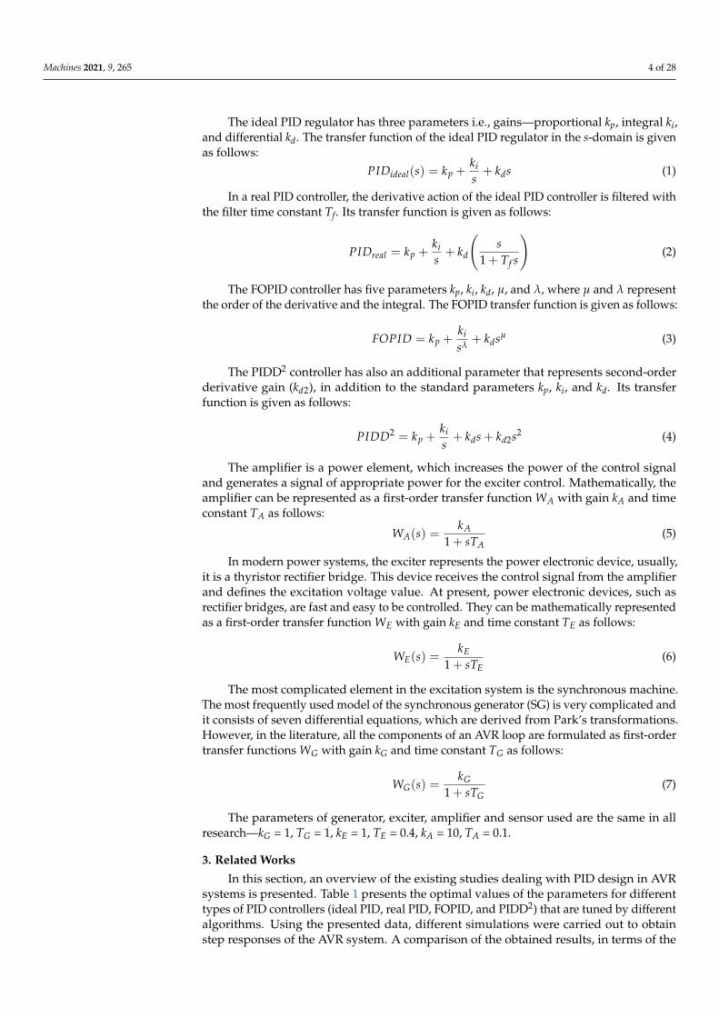
All previously determined results (PIDD2 design) were realized using the proposedEO–ERWCA algorithm. To demonstrate its power and superiority over other algorithms,a comparison between the proposed algorithm and other algorithms in the literature(WOA [5], YSGA [30], CS [19], and SA-MRFA [17]) is made in terms of the convergencespeed. The number of runs in all algorithms was set to 30, and the normalized meanvalue of the convergence curves is presented in Figure 18. Additionally, each algorithmwas employed to the optimal tuning of the real PID controller using the same settings asthe proposed algorithm. It is obvious in Figure 18 that the EO-ERWCA converges to theoptimal solution faster than other algorithms.

Machines 2021, 9, 265 21 of 28Machines 2021, 9, x FOR PEER REVIEW 22 of 28

Figure 18. Mean results of the convergence characteristics over 30 independent runs.

Moreover, it is well known that metaheuristic algorithms have a stochastic nature.

For that reason, the considered algorithms had 30 independent runs and the best, worst,

mean, and median values are calculated and presented in Table 3. Additionally, the stand-

ard deviation of the presented results was calculated. It is clear from Table 3 that the stand-

ard deviation has the lowest value when the proposed EO-ERWCA algorithm is applied.

It can be concluded that the deviation of the results obtained from each run is very small,

so the results obtained are consistent. In addition to the previous statistical analysis

measures, a non-parametric statistical test called Wilcoxon’s rank-sum test was also car-

ried out. This test enables additional comparison between the proposed EO–ERWCA al-

gorithm and CS, WOA, and YSGA algorithms. The corresponding p-values obtained by

applying this test are presented in Table 4 with a 5% level of significance between the EO–

ERWCA and other optimization methods. The proposed algorithm is clearly effective,

fast, and accurate.

Table 3. Statistical measures of the results obtained with the different algorithms.

Algorithm Best Worst Mean Median Standard Deviation

EO-ERWCA 1284.5 1406.9 1345.1 1343.0 35.7286

YSGA 1284.7 1468.6 1378.4 1381.3 54.2141

CS 1284.6 1592.0 1429.7 1427.2 110.1038

WOA 1286.4 1530.8 1415.7 1424.6 70.0808

Table 4. p-values obtained with Wilcoxon’s rank-sum test.

Algorithms EO–ERWCA vs. CS EO–ERWCA vs. WOA EO–ERWCA vs. YSGA

p-value 4.4034 × 10−20 3.1748 × 10−19 3.3537 × 10−12

6. Experimental Results

The previously presented simulations show that the limitation of the excitation volt-

age leads to a slower generator voltage change. In addition, the lower values of the regu-

lator parameters provide a lower value of the excitation voltage. These analyses were the

starting point for an experimental investigation of the proposed controller design. The

Figure 18. Mean results of the convergence characteristics over 30 independent runs.

Moreover, it is well known that metaheuristic algorithms have a stochastic nature. Forthat reason, the considered algorithms had 30 independent runs and the best, worst, mean,and median values are calculated and presented in Table 3. Additionally, the standarddeviation of the presented results was calculated. It is clear from Table 3 that the standarddeviation has the lowest value when the proposed EO-ERWCA algorithm is applied. It canbe concluded that the deviation of the results obtained from each run is very small, so theresults obtained are consistent. In addition to the previous statistical analysis measures, anon-parametric statistical test called Wilcoxon’s rank-sum test was also carried out. Thistest enables additional comparison between the proposed EO–ERWCA algorithm and CS,WOA, and YSGA algorithms. The corresponding p-values obtained by applying this testare presented in Table 4 with a 5% level of significance between the EO–ERWCA and otheroptimization methods. The proposed algorithm is clearly effective, fast, and accurate.

Table 3. Statistical measures of the results obtained with the different algorithms.

Algorithm Best Worst Mean Median StandardDeviation

EO-ERWCA 1284.5 1406.9 1345.1 1343.0 35.7286YSGA 1284.7 1468.6 1378.4 1381.3 54.2141

CS 1284.6 1592.0 1429.7 1427.2 110.1038WOA 1286.4 1530.8 1415.7 1424.6 70.0808

Table 4. p-Values obtained with Wilcoxon’s rank-sum test.

Algorithms EO–ERWCA vs. CS EO–ERWCA vs.WOA

EO–ERWCA vs.YSGA

p-value 4.4034 × 10−20 3.1748 × 10−19 3.3537 × 10−12

6. Experimental Results

The previously presented simulations show that the limitation of the excitation voltageleads to a slower generator voltage change. In addition, the lower values of the regulatorparameters provide a lower value of the excitation voltage. These analyses were the

Machines 2021, 9, 265 22 of 28

starting point for an experimental investigation of the proposed controller design. Theexperimental verification of the impact of excitation controller parameters value as wellas of the excitation voltage value on the generator voltage was realized using a lead-lagcompensator on one 120 MVA 15.75 kV, 50 Hz generator from HPP Piva, Montenegro,as shown in Figure 19a. The excitation system in HPP Piva is called Thyricon, which ismanufactured by Voith Siemens. It is a thyristor-controlled self-excitation system. Thecontrol of the excitation voltage, besides the voltage control loop, includes other controlloops such as excitation current, power system stabilizer, generator current, and others.In that way, the regulation of the generator voltage includes all the vital control variables.The regulation of the generator voltage was realized using a lead-lag compensator. Theblock diagram of the AVR control is presented in Figure 19b, where Ug-ref represents thegenerator reference value, while Ug-meas represents the generator measured voltage.

The lead-lag compensator, whose transfer function is WR(s), is realized in the followingmanner:

WR(s) =1 + sTC1

1 + sTB1× 1 + sTC2

1 + sTB2× KR

GR(29)

where TB1,2 and TC1,2 are time constants, KR is the proportional gain, and GR is the gain ofthe rectifier. The corresponding Bode characteristic of the lead-lag compensator is presentedin Figure 19c.

These parameters are expressed as follows:

KR = V0, TB1 =TaV0Vp

TC1 = Ta, TB2 =TbVpV00

, TC2 = Tb (30)

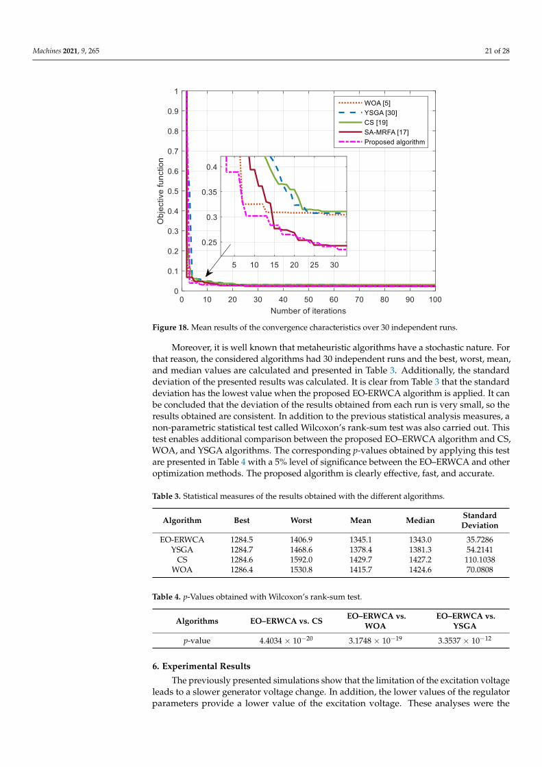
The generator is accelerated at the nominal speed and excited in no-load operationwith a 0.947 p.u voltage value. After 7 s, the reference generator voltage set-point is changedto 1.046 p.u. A command is added to the excitation voltage to increase the generator voltage.Finally, after 6 s, the reference generator voltage is changed to the first value (0.947 p.u).This experiment is realized for two different values of lead-lag compensator parameters. Inthe first experiment, the lead-lag compensator parameters are Ta = 1.5 s, Tb = 0.1 s, Vp = 60,V0 = 250, and V00 = 50. In the second experiment, the lead-lag compensator parameters areTa = 0.75 s, Tb = 0.05 s, Vp = 30, V0 = 250, and V00 = 50. The measurements were realizedduring July 2020 and refined in October 2021. For recording measurements, UNITROLUN6080 (SW version: 2.1.0.8), type: A6T-A/08T1-A1250, UN 6080 2CH was used. Thecorresponding results are presented in Figure 20.

Machines 2021, 9, 265 23 of 28

Machines 2021, 9, x FOR PEER REVIEW 23 of 28

experimental verification of the impact of excitation controller parameters value as well

as of the excitation voltage value on the generator voltage was realized using a lead-lag

compensator on one 120 MVA 15.75 kV, 50 Hz generator from HPP Piva, Montenegro, as

shown in Figure 19a. The excitation system in HPP Piva is called Thyricon, which is man-

ufactured by Voith Siemens. It is a thyristor-controlled self-excitation system. The control

of the excitation voltage, besides the voltage control loop, includes other control loops

such as excitation current, power system stabilizer, generator current, and others. In that

way, the regulation of the generator voltage includes all the vital control variables. The

regulation of the generator voltage was realized using a lead-lag compensator. The block

diagram of the AVR control is presented in Figure 19b, where Ug-ref represents the genera-

tor reference value, while Ug-meas represents the generator measured voltage.

(a)

(b)

(c)

Figure 19. Experimental setup: (a) 120 MVA generator from HPP Piva, (b) AVR model in HPP Piva,

(c) Bode characteristic of the lead-lag compensator.

Figure 19. Experimental setup: (a) 120 MVA generator from HPP Piva, (b) AVR model in HPP Piva,(c) Bode characteristic of the lead-lag compensator.

The sudden change of the generator voltage set-point leads to a sudden rise of theexcitation voltage. This very fast change enables the thyristor bridge operation in the

Machines 2021, 9, 265 24 of 28

static excitation system. The rise of the excitation voltage leads to the rise of the excitationcurrent, and finally leads to the rise of output generator voltage.

On the opposite side, when the generator voltage set-point suddenly decreases, theexcitation voltage suddenly decreases, which results in a reduction of the excitation currentand voltage at the ends of the generator. In the second experiment, as lower lead-lagcompensator parameters are implemented, the voltage response of the generator wasslower. This is a consequence of the slower and smaller growth of the excitation current.Furthermore, in this case, forcing the field current after the initial rise was slower, asillustrated in Figure 20b. Therefore, the lower value of lead-lag compensator parametersprovides a slower change of the generator voltage. It was also clear that higher valuesof lead-lag compensator parameters, i.e., a higher value of the excitation voltage causessmaller rise time and settling time of the generator voltage during step change. To sum up,it can be concluded that the value of lead-lag compensator parameters has considerableeffects on the excitation voltage, excitation current, and generator voltage waveforms.

Machines 2021, 9, x FOR PEER REVIEW 24 of 28

The lead-lag compensator, whose transfer function is WR(s), is realized in the follow-

ing manner:

𝑊𝑅(𝑠) = 1 + 𝑠𝑇𝐶1

1 + 𝑠𝑇𝐵1

×1 + 𝑠𝑇𝐶2

1 + 𝑠𝑇𝐵2

×𝐾𝑅

𝐺𝑅 (29)

where TB1,2 and TC1,2 are time constants, KR is the proportional gain, and GR is the gain

of the rectifier. The corresponding Bode characteristic of the lead-lag compensator is pre-

sented in Figure 19c.

These parameters are expressed as follows:

𝐾𝑅 = 𝑉0, 𝑇𝐵1 = 𝑇𝑎

𝑉0𝑉𝑝

⁄

𝑇𝐶1 = 𝑇𝑎, 𝑇𝐵2 = 𝑇𝑏

𝑉𝑝𝑉00

⁄, 𝑇𝐶2 = 𝑇𝑏

(29)

The generator is accelerated at the nominal speed and excited in no-load operation

with a 0.947 p.u voltage value. After 7 s, the reference generator voltage set-point is

changed to 1.046 p.u. A command is added to the excitation voltage to increase the gen-

erator voltage. Finally, after 6 s, the reference generator voltage is changed to the first

value (0.947 p.u). This experiment is realized for two different values of lead-lag compen-

sator parameters. In the first experiment, the lead-lag compensator parameters are Ta = 1.5

s, Tb = 0.1 s, Vp = 60, V0 = 250, and V00 = 50. In the second experiment, the lead-lag compen-

sator parameters are Ta = 0.75 s, Tb = 0.05 s, Vp = 30, V0 = 250, and V00 = 50. The measurements

were realized during July 2020 and refined in October 2021. For recording measurements,

UNITROL UN6080 (SW version: 2.1.0.8), type: A6T-A/08T1-A1250, UN 6080 2CH was

used. The corresponding results are presented in Figure 20.

(a)

Figure 20. Cont.

Machines 2021, 9, 265 25 of 28

Machines 2021, 9, x FOR PEER REVIEW 25 of 28

(b)

(c)

Figure 20. Experimental results: (a) field voltage (b) field current, and (c) generator voltage.

The sudden change of the generator voltage set-point leads to a sudden rise of the

excitation voltage. This very fast change enables the thyristor bridge operation in the static

excitation system. The rise of the excitation voltage leads to the rise of the excitation cur-

rent, and finally leads to the rise of output generator voltage.

Figure 20. Experimental results: (a) field voltage (b) field current, and (c) generator voltage.

Machines 2021, 9, 265 26 of 28

7. Conclusions

This paper addressed the design of regulators in AVR systems, as well as the experi-mental verification of the impact of the optimal regulator parameters on the generator. Tothis end, the importance of taking the value of the excitation voltage into account whendesigning parameters of the AVR system controller was first discussed. Additionally, acomparison of system responses of different controller parameters found in the literaturewas performed. Analyzing the obtained results, it was concluded that the PIDD2 controllerallows the minimum delay time and rise time of the generator voltage. Therefore, theparameters of the PIDD2 controller were estimated and the excitation voltage values weremonitored. Besides, two new optimization functions and a novel hybrid metaheuristicalgorithm are proposed in the paper. Analyzing the obtained results using them, it wasconcluded that limiting the values of the excitation voltage leads to a decrease in the valuesof the optimal parameters of the regulator. Based on this conclusion, the influence ofthe values of the regulator parameters on the response of the excitation voltage and thegenerator voltage in HPP Piva was investigated. The experimental results validated theconclusions figured out from the simulation studies that limiting the maximum valueof the excitation voltage leads to a higher value of the rise time and the rise time of thegenerator voltage. Finally, the determination of AVR controller parameters by applying theanti-windup type of excitation voltage limitation will be considered in future works.

In future work, the parameters of synchronous generators of HPP PIVA will beestimated to simulate the AVR system for generators of the same power plant. In thisway, it will be possible to easily test different types and values of regulator parameters toachieve the desired generator voltage responses.

Author Contributions: Conceptualization, M.C. and M.M.; methodology, M.C.; software, M.M. andM.R.; validation, M.C., A.F.Z., H.M.H. and S.H.E.A.A.; formal analysis, M.C.; investigation, M.R.;writing—original draft preparation, M.C., M.M. and S.H.E.A.A.; writing—review and editing, A.F.Z.,H.M.H. and S.H.E.A.A.; visualization, M.M. and M.R. All authors have read and agreed to thepublished version of the manuscript.

Funding: This research received no external funding.

Institutional Review Board Statement: Not applicable.

Informed Consent Statement: Not applicable.

Data Availability Statement: The data presented in this study are available upon request from thecorresponding author. The data are not publicly available due to their large size.

Acknowledgments: The authors acknowledge with thanks the HPP Piva, Montenegro for theirtechnical and financial support.

Conflicts of Interest: The authors declare no conflict of interest.

References1. Murty, P.S.R. Operation and Control in Power Systems, 1st ed.; BSP Publications: Hyderabad, India, 2008.2. Boldea, I. Synchronous Generators, 2nd ed.; CRC Press: Boca Raton, FL, USA, 2016.3. Lipo, T.A. Analysis of Synchronous Machines, 2nd ed.; CRC Press: Boca Raton, FL, USA, 2012.4. Ekinci, S.; Hekimoglu, B. Improved Kidney-Inspired Algorithm Approach for Tuning of PID Controller in AVR System. IEEE

Access 2019, 7, 39935–39947. [CrossRef]5. Mosaad, A.M.; Attia, M.A.; Abdelaziz, A.Y. Whale optimization algorithm to tune PID and PIDA controllers on AVR system. Ain

Shams Eng. J. 2019, 10, 755–767. [CrossRef]6. Çelik, E.; Durgut, R. Performance enhancement of automatic voltage regulator by modified cost function and symbiotic organisms

search algorithm. Eng. Sci. Technol. Int. J. 2018, 21, 1104–1111. [CrossRef]7. Mosaad, A.M.; Attia, M.A.; Abdelaziz, A.Y. Comparative Performance Analysis of AVR Controllers Using Modern Optimization

Techniques. Electr. Power Compon. Syst. 2018, 46, 2117–2130. [CrossRef]8. Blondin, M.J.; Sanchis, J.; Sicard, P.; Herrero, J.M. New optimal controller tuning method for an AVR system using a simplified

Ant Colony Optimization with a new constrained Nelder–Mead algorithm. Appl. Soft Comput. J. 2018, 62, 216–229. [CrossRef]

Machines 2021, 9, 265 27 of 28

9. Mohanty, P.K.; Sahu, B.K.; Panda, S. Tuning and assessment of proportional-integral-derivative controller for an automatic voltageregulator system employing local unimodal sampling algorithm. Electr. Power Compon. Syst. 2014, 42, 959–969. [CrossRef]

10. Hasanien, H.M. Design optimization of PID controller in automatic voltage regulator system using taguchi combined geneticalgorithm method. IEEE Syst. J. 2013, 7, 825–831. [CrossRef]

11. Panda, S.; Sahu, B.K.; Mohanty, P.K. Design and performance analysis of PID controller for an automatic voltage regulator systemusing simplified particle swarm optimization. J. Frankl. Inst. 2012, 349, 2609–2625. [CrossRef]

12. Kim, D.H. Hybrid GA–BF based intelligent PID controller tuning for AVR system. Appl. Soft. Comput. 2011, 11, 11–22. [CrossRef]13. Gozde, H.; Taplamacioglu, M.C. Comparative performance analysis of artificial bee colony algorithm for automatic voltage

regulator (AVR) system. J. Frankl. Inst. 2011, 348, 1927–1946. [CrossRef]14. dos Santos Coelho, L. A quantum particle swarm optimizer with chaotic mutation operator. Chaos Solitons Fractals 2008, 37,

1409–1418. [CrossRef]15. Gaing, Z.-L. A Particle Swarm Optimization Approach for Optimum Design of PID Controller in AVR System. IEEE Trans. Energy

Convers. 2004, 19, 384–491. [CrossRef]16. Micev, M.; Calasan, M.; Oliva, D. Design and robustness analysis of an Automatic Voltage Regulator system controller by using

Equilibrium Optimizer algorithm. Comput. Electr. Eng. 2021, 89, 106930. [CrossRef]17. Micev, M.; Calasan, M.; Ali, Z.M.; Hasanien, H.M.; Abdel Aleem, S.H.A. Optimal Design of Automatic Voltage Regulation

Controller Using Hybrid Simulated Annealing—Manta Ray Foraging Optimization Algorithm. Ain Shams Eng. J. 2021, 12,641–657. [CrossRef]

18. Blondin, M.J.; Sicard, P.; Pardalos, P.M. Controller Tuning Approach with robustness, stability and dynamic criteria for theoriginal AVR System. Math. Comput. Simul. 2019, 163, 168–182. [CrossRef]

19. Bingul, Z.; Karahan, O. A novel performance criterion approach to optimum design of PID controller using cuckoo searchalgorithm for AVR system. J. Frankl. Inst. 2018, 355, 5534–5559. [CrossRef]

20. Chatterjee, S.; Mukherjee, V. PID controller for automatic voltage regulator using teaching-learning based optimization technique.Int. J. Electr. Power Energy Syst. 2016, 77, 418–429. [CrossRef]

21. Sahib, M.A.; Ahmed, B.S. A new multiobjective performance criterion used in PID tuning optimization algorithms. J. Adv. Res.2016, 7, 125–134. [CrossRef] [PubMed]

22. Pan, I.; Das, S. Frequency domain design of fractional order PID controller for AVR system using chaotic multi-objectiveoptimization. Int. J. Electr. Power Energy Syst. 2013, 51, 106–118. [CrossRef]

23. Zhang, D.L.; Tang, Y.-G.; Guan, X.-P. Optimum Design of Fractional Order PID Controller for an AVR System Using an ImprovedArtificial Bee Colony Algorithm. Acta Autom. Sin. 2014, 40, 973–979. [CrossRef]

24. Tang, Y.; Cui, M.; Hua, C.; Li, L.; Yang, Y. Optimum design of fractional order PI λD µ controller for AVR system using chaotic antswarm. Expert Syst. Appl. 2012, 39, 6887–6896. [CrossRef]

25. Pan, I.; Das, S. Chaotic multi-objective optimization based design of fractional order PI λD µ controller in AVR system. Int. J.Electr. Power Energy Syst. 2012, 43, 393–407. [CrossRef]

26. Zeng, G.Q.; Chen, J.; Dai, Y.X.; Li, L.M.; Zheng, C.W.; Chen, M.R. Design of fractional order PID controller for automatic regulatorvoltage system based on multi-objective extremal optimization. Neurocomputing 2015, 160, 173–184. [CrossRef]

27. Sikander, A.; Thakur, P.; Bansal, R.C.; Rajasekar, S. A novel technique to design cuckoo search based FOPID controller for AVR inpower systems. Comput. Electr. Eng. 2018, 70, 261–274. [CrossRef]

28. Ortiz-Quisbert, M.E.; Duarte-Mermoud, M.A.; Milla, F.; Castro-Linares, R.; Lefranc, G. Optimal fractional order adaptivecontrollers for AVR applications. Electr. Eng. 2018, 100, 267–283. [CrossRef]

29. Khan, I.A.; Alghamdi, A.S.; Jumani, T.A.; Alamgir, A.; Awan, A.B.; Khidrani, A. Salp Swarm Optimization Algorithm-BasedFractional Order PID Controller for Dynamic Response and Stability Enhancement of an Automatic Voltage Regulator System.Electronics 2019, 8, 1472. [CrossRef]

30. Micev, M.; Calasan, M.; Oliva, D. Fractional Order PID Controller Design for an AVR System Using Chaotic Yellow SaddleGoatfish Algorithm. Mathematics 2020, 8, 1182. [CrossRef]

31. Sahib, M.A. A novel optimal PID plus second order derivative controller for AVR system. Eng. Sci. Technol. Int. J. 2015, 18,194–206. [CrossRef]

32. Zamani, M.; Karimi-Ghartemani, M.; Sadati, N.; Parniani, M. Design of a fractional order PID controller for an AVR using particleswarm optimization. Control Eng. Pract. 2009, 17, 1380–1387. [CrossRef]

33. Calasan, M.; Micev, M.; Djurovic, Z.; Mageed, H.M.A. Artificial ecosystem-based optimization for optimal tuning of robustPID controllers in AVR systems with limited value of excitation voltage. Inter. J. Electr. Eng. Educ. 2020, 1, 0020720920940605.[CrossRef]

34. Migallón, H.; Belazi, A.; Sánchez-Romero, J.L.; Rico, H.; Jimeno-Morenilla, A. Settings-free hybrid metaheuristic generaloptimization methods. Mathematics 2020, 8, 1092. [CrossRef]

35. Faramarzi, A.; Heidarinejad, M.; Stephens, B.; Mirjalili, S. Equilibrium optimizer: A novel optimization algorithm. Knowl.-BasedSyst. 2020, 191, 105190. [CrossRef]

36. Sadollah, A.; Eskandar, H.; Bahreininejad, A.; Kim, J.H. Water cycle algorithm with evaporation rate for solving constrained andunconstrained optimization problems. Appl. Soft Comput. J. 2015, 30, 58–71. [CrossRef]

Machines 2021, 9, 265 28 of 28

37. Calasan, M.; Micev, M.; Ali, Z.M.; Zobaa, A.F.; Abdel Aleem, S.H. Parameter Estimation of Induction Machine Single-Cage andDouble-Cage Models Using a Hybrid Simulated Annealing–Evaporation Rate Water Cycle Algorithm. Mathematics 2020, 8, 1024.[CrossRef]

38. Kler, D.; Sharma, P.; Banerjee, A.; Rana, K.P.S.; Kumar, V. PV cell and module efficient parameters estimation using EvaporationRate-based Water Cycle Algorithm. Swarm Evol. Comput. 2017, 35, 93–110. [CrossRef]