Journal of Advanced Research (2012) 3, 225–232

Cairo University

Journal of Advanced Research

ORIGINAL ARTICLE

Design of aerospace control systems using fractional

PID controller

Magdy A.S. Aboelela b,*, Mohamed F. Ahmed a, Hassen T. Dorrah b

a Egyptian Armed Forces, Cairo, Egyptb Cairo University, Faculty of Engineering, Electric Power and Machines Department, Giza, Egypt

Received 20 February 2011; revised 23 May 2011; accepted 4 July 2011Available online 16 September 2011

*

E-

20

El

Pe

do

KEYWORDS

Six degree of freedom missile

model;

Particle swarm optimization;

Fractional PID control;

Matlab/Simulink

Corresponding author. Tel.:

mail address: magdysafaa@y

90-1232 ª 2011 Cairo Un

sevier B.V. All rights reserve

er review under responsibilit

i:10.1016/j.jare.2011.07.003

Production and h

+20 012

ahoo.com

iversity.

d.

y of Cair

osting by E

Abstract The goal is to control the trajectory of the flight path of six degree of freedom flying body

model using fractional PID. The design of fractional PID controller for the six degree of freedom

flying body is described. The parameters of fractional PID controller are optimized by particle

swarm optimization (PSO) method. In the optimization process, various objective functions were

considered and investigated to reflect both improved dynamics of the missile system and reduced

chattering in the control signal of the controller.ª 2011 Cairo University. Production and hosting by Elsevier B.V. All rights reserved.

Introduction and literature review

In recent years, the requirements for the quality of automaticcontrol increased significantly due to increased complexity ofplants and sharper specifications of product. This paper willaddress the design of optimal variable structure controllers ap-

plied to a six degree of freedom missile model which is the solu-tion to obtain a detailed accurate data about the missiletrajectory. The paper objectives are: (a) to develop a general

3781585.

(M.A.S. Aboelela).

Production and hosting by

o University.

lsevier

flexible sophisticated mathematical model of flight trajectorysimulation for a hypothetical anti-tank missile, which can beused as a base line algorithm contributing for design, analysis,

and development of such a system and implement this modelusing Simulink to facilitate the design of its control system,and (b) developing control system, by using fractional PID

control techniques.According to MacKenzie, guidance is defined as the process

for guiding the path of an object toward a given point, which

in general is moving [1]. Furthermore, the father of inertialnavigation, Charles Stark Draper, states that ‘‘Guidance de-pends upon fundamental principles and involves devices thatare similar for vehicles moving on land, on water, under water,

in air, beyond the atmosphere within the gravitational field ofearth and in space outside this field’’ [2]. The most rich andmature literature on guidance is probably found within the

guided missile community. A guided missile is defined as aspace-traversing unmanned vehicle that carries within itselfthe means for controlling its flight path [3]. Guided missiles

have been operational since World War II [1]. Today, missileguidance theory encompasses a broad spectrum of guidance

Nomenclature

Cx drag coefficient

Cy lift coefficientCz lateral coefficientD diameter of maximum cross-section area (m)Fx, Fy, Fz components of total forces acting on missile (N)

F fitness functionG gravity force (N)Gx, Gy, Gz gravity force components (N)

I moment of inertia (kg m2/s)Ix, Iy, Iz moment of inertia components (kg m2/s)J cost function (objective function)

kp proportional gainki integral gainkd derivative gainMTHx, MTHy, MTHz thrust moment components (N m)

MAx, MAy, MAz aerodynamic moment components (N m)Mx, My, Mz components of total moments acting on mis-

sile (N m)

m the mass of missile (kg)mx0, myb, my0, mza, mz0 aerodynamic moment coefficientsRx, Ry, Rz aerodynamic force components (N)

r reference signal

S reference area (m2)T thrust force (N)Tx, Ty, Tz thrust force components (N)Vm missile velocity (m/s)

w weight factorX range of missile (m)Xg, Yg, Zg ground coordinate

Xb, Yb, Zb body coordinateXV, YV, ZV velocity coordinateXcg distance between cg and the nozzle (m)

U, W, c Euler’s angles (�)Up pitch demand programmer (�)Wp yaw demand programmer (�)a, b angles of attack (�)d fractional derivativeda jet deflection angle in the pitch plane (�)db jet deflection angle in the yaw plane (�)k fractional integrationxx;xy;xz angular velocity components (rad/s)

226 M.A.S. Aboelela et al.

laws as classical guidance laws, optimal guidance laws, guid-

ance laws based on fuzzy logic and neural network theory, dif-ferential geometric guidance laws and guidance laws based ondifferential game theory. Very interesting personal accounts of

the guided missile development during and after World War IIcan be found in the literature [5,7,9]. Moreover, Locke andWestrum put the development of guided missile technology

into a larger perspective [10,15].

Methodology

Mathematical model of the missile

The model constitutes the six degree of freedom (6-DOF)equations that break down into those describing kinematics,dynamics (aerodynamics, thrust, and gravity), command guid-

ance generation systems, and autopilot (electronics, instru-ments, and actuators). The input to this model is launchconditions, target motion, and target trajectory characteriza-

tion, while the outputs are the missile flight data (speed, accel-eration, range, etc.) during engagement.

The basic frames needed for subsequent analytical develop-

ments are the ground, body and velocity coordinate systems.The origins of these coordinate systems are the missile centerof gravity (cg). In the ground coordinate system, the Xg–Zg

lie in the horizontal plane and the Yg axis completes a standard

right-handed system and points up vertically. In the bodycoordinate system, the positive Xb axis coincides with the mis-sile’s center line and it is designated as roll-axis. The positive

Zb axis is to the right of the Xb axis in the horizontal planeand it is designated as the pitch axis. The positive Yb axispoints upward and it is designed as the yaw axis. The body axis

system is fixed with respect to the missile and moves with themissile. In the velocity coordinate system, XV coincides with

the direction of missile velocity (Vm), which related to the

directions of missile flight. The axis ZV completes a standardright-handed system [4,6].

The pitch plane is X–Y plane, the yaw plane is X–Z plane,

and the roll plane is Y–Z plane. The ground coordinate systemand body coordinate system are related to each other throughEuler’s angles (U, W, c). The ground coordinate system and

velocity coordinate system are related to each other throughthe angles (h, r). In addition, the velocity coordinate systemis related to the body frame through the angle of attack (a)in the pitch plane and sideslip angle (b) in the yaw plane.

The angles between different coordinate systems are shownin Fig. 1a [4,6].

The relation between the body and the velocity coordinate

systems can be given as follows:

Xb

Yb

Zb

264

375 ¼ cosðaÞ cosðbÞ sinðaÞ � cosðaÞ sinðbÞ

� sinðaÞ cosðbÞ cosðaÞ sinðaÞ sinðbÞsinðbÞ0 cosðbÞ

� � XV

YV

ZV

264

375ð1Þ

The body and velocity axes system as well as forces, momentsand other quantities are shown in Fig. 1b.

There are 6 dynamic equations (3 for translational motion

and 3 for rotational motion) and 6 kinematic equations (3for translational motion and 3 for rotational motion) for amissile with six degrees of freedom. The equations are some-

what simpler, if the mass is constant. The missile 6-DOF equa-tions in velocity coordinate system are given as following [4]:

Fx ¼ m _Vm ð2Þ

Fy ¼ mVm_h ð3Þ

Fz ¼ �mVm cosðhÞ _r ð4Þ

Fig. 1b Forces, moments and other quantities.

Fig. 1a The angles between different coordinate systems.

Control of aerospace using FOPID 227

Mx ¼ Ix _xx � ðIy � IzÞxyxz ð5Þ

My ¼ Iy _xy � ðIz � IxÞxzxx ð6Þ

Mz ¼ Iz _xz � ðIx � IyÞxxxy ð7Þ

_X ¼ Vm cosðhÞ cosðrÞ ð8Þ

_Y ¼ Vm sinðhÞ ð9Þ

_Z ¼ �Vm cosðhÞ sinðrÞ ð10Þ

_W ¼ ðxy cosðcÞ � xz sinðcÞÞ= cosðUÞ ð11Þ

_U ¼ xy sinðcÞ þ xz cosðcÞ ð12Þ

_c ¼ xx � tanðUÞðxy cosðcÞ � xz sinðcÞÞ ¼ xx � _W sinðUÞ ð13Þ

In these equations, Fx, Fy, Fz are components of forces act-ing on missile in velocity coordinate system; Mx, My, Mz are

moments acting on missile in body coordinate system; xx,xy, xz are angular velocity in body coordinate system; Ix, Iy,Iz are moments of inertia in body coordinate system; X is mis-sile range; Y is missile altitude; Z is horizontal displacement of

the missile; and m is missile mass. The forces and the momentsacting on missile are due to thrust, aerodynamic and gravitythat are given as following [4,6,8]:

Fx ¼ T cosða� daÞ cosðb� dbÞ �QSðCx0 þ Cxða2 þ b2ÞÞ�mg sinðhÞ ð14Þ

Fy ¼ T sinða� daÞ þQSCya�mg cosðhÞ ð15Þ

Fz ¼ �T cosða� daÞ sinðb� dbÞ �QSCzb ð16Þ

Mx ¼ DQSmx0

xxD

2Vm

ð17Þ

My ¼ �T cosðdaÞ sinðdbÞXcg þDQS mybbþmy0

xyD

Vm

� �ð18Þ

Mz ¼ T sinðdaÞXcg þDQS mzabþmz0

xzD

Vm

� �ð19Þ

In these equations, Cx, Cx0, Cy, Cz are aerodynamic forcecoefficient; mx0, myb, my0, mza, mz0 are aerodynamic moment

coefficients; D is the diameter of maximum cross-section areaof body; S is the reference area; Q is the dynamic pressure;da is the nozzle deflection angle in the pitch plane; db is the noz-

zle deflection angle in the yaw plane; T is the thrust force; Xcg

is the distance between the center of gravity (cg) and the noz-zle; and g is acceleration due to gravity and is taken to be con-

stant 9.81 m/s2.

Fractional order PID controller design

In recent years, researchers reported that controllers makinguse of factional order derivatives and integrals could achieveperformance and robustness results superior to those ob-

tained with conventional (integer order) controllers. Thefractional-order PID controller (FOPID) is the expansionof the conventional PID controller based on fractional

calculus.

Theory of fractional calculus

The fractional calculus is a generalization of integration andderivation to non-integer order operator. We use the general-ization of the differential and integral operators into one fun-

damental operator aDat where

aDat fðtÞ ¼

dafðtÞdta

for RðaÞ > 0

1 for RðaÞ ¼ 0R t

afðsÞðdsÞ�a

for RðaÞ < 0

8><>: ð20Þ

RðaÞ denotes the real part of calculus order a which is a

complex quantity. For our purpose, a is purely real a and tare the limits related to the operation of fractional differentia-tion [11,13].

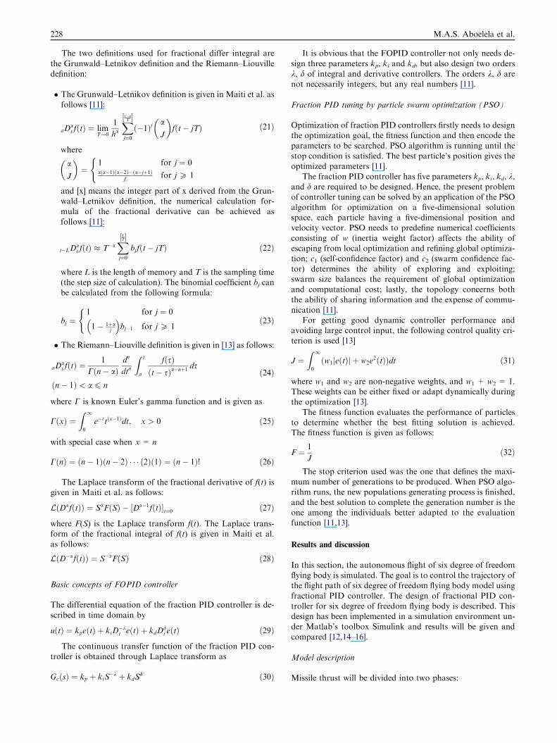
228 M.A.S. Aboelela et al.

The two definitions used for fractional differ integral are

the Grunwald–Letnikov definition and the Riemann–Liouvilledefinition:

� The Grunwald–Letnikov definition is given in Maiti et al. as

follows [11]:

aDat fðtÞ ¼ lim

T!0

1

ha

Xt�aT½ �j¼0ð�1Þj

a

J

� �fðt� jTÞ ð21Þ

where

a

J

� �¼

1 for j ¼ 0aða�1Þða�2Þ���ða�jþ1Þ

j!for j P 1

(

and [x] means the integer part of x derived from the Grun-wald–Letnikov definition, the numerical calculation for-

mula of the fractional derivative can be achieved asfollows [11]:

t�LDat fðtÞ � T�a

XLT½ �

j¼0bjfðt� jTÞ ð22Þ

where L is the length of memory and T is the sampling time(the step size of calculation). The binomial coefficient bj can

be calculated from the following formula:

bj ¼1 for j ¼ 0

1� 1þaj

� �bj�1 for j P 1

(ð23Þ

� The Riemann–Liouville definition is given in [13] as follows:

aDat fðtÞ ¼

1

Cðn� aÞdn

dtn

Z t

a

fðsÞðt� sÞa�nþ1

ds

ðn� 1Þ < a 6 n

ð24Þ

where C is known Euler’s gamma function and is given as

CðxÞ ¼Z 1

0

e�ttðx�1Þdt; x > 0 ð25Þ

with special case when x = n

CðnÞ ¼ ðn� 1Þðn� 2Þ � � � ð2Þð1Þ ¼ ðn� 1Þ! ð26Þ

The Laplace transform of the fractional derivative of f(t) isgiven in Maiti et al. as follows:

LðDafðtÞÞ ¼ SaFðSÞ � ½Da�1fðtÞ�t¼0 ð27Þ

where F(S) is the Laplace transform f(t). The Laplace trans-form of the fractional integral of f(t) is given in Maiti et al.as follows:

LðD�afðtÞÞ ¼ S�aFðSÞ ð28Þ

Basic concepts of FOPID controller

The differential equation of the fraction PID controller is de-

scribed in time domain by

uðtÞ ¼ kpeðtÞ þ kiD�kt eðtÞ þ kdD

dt eðtÞ ð29Þ

The continuous transfer function of the fraction PID con-

troller is obtained through Laplace transform as

GcðsÞ ¼ kp þ kiS�k þ kdS

d ð30Þ

It is obvious that the FOPID controller not only needs de-

sign three parameters kp, ki and kd, but also design two ordersk, d of integral and derivative controllers. The orders k, d arenot necessarily integers, but any real numbers [11].

Fraction PID tuning by particle swarm optimization (PSO)

Optimization of fraction PID controllers firstly needs to design

the optimization goal, the fitness function and then encode theparameters to be searched. PSO algorithm is running until thestop condition is satisfied. The best particle’s position gives the

optimized parameters [11].The fraction PID controller has five parameters kp, ki, kd, k,

and d are required to be designed. Hence, the present problem

of controller tuning can be solved by an application of the PSOalgorithm for optimization on a five-dimensional solutionspace, each particle having a five-dimensional position andvelocity vector. PSO needs to predefine numerical coefficients

consisting of w (inertia weight factor) affects the ability ofescaping from local optimization and refining global optimiza-tion; c1 (self-confidence factor) and c2 (swarm confidence fac-

tor) determines the ability of exploring and exploiting;swarm size balances the requirement of global optimizationand computational cost; lastly, the topology concerns both

the ability of sharing information and the expense of commu-nication [11].

For getting good dynamic controller performance andavoiding large control input, the following control quality cri-

terion is used [13]

J ¼Z 1

0

ðw1jeðtÞj þ w2e2ðtÞÞdt ð31Þ

where w1 and w2 are non-negative weights, and w1 + w2 = 1.These weights can be either fixed or adapt dynamically duringthe optimization [13].

The fitness function evaluates the performance of particlesto determine whether the best fitting solution is achieved.The fitness function is given as follows:

F ¼ 1

Jð32Þ

The stop criterion used was the one that defines the maxi-mum number of generations to be produced. When PSO algo-rithm runs, the new populations generating process is finished,

and the best solution to complete the generation number is theone among the individuals better adapted to the evaluationfunction [11,13].

Results and discussion

In this section, the autonomous flight of six degree of freedomflying body is simulated. The goal is to control the trajectory ofthe flight path of six degree of freedom flying body model using

fractional PID controller. The design of fractional PID con-troller for six degree of freedom flying body is described. Thisdesign has been implemented in a simulation environment un-der Matlab’s toolbox Simulink and results will be given and

compared [12,14–16].

Model description

Missile thrust will be divided into two phases:

Control of aerospace using FOPID 229

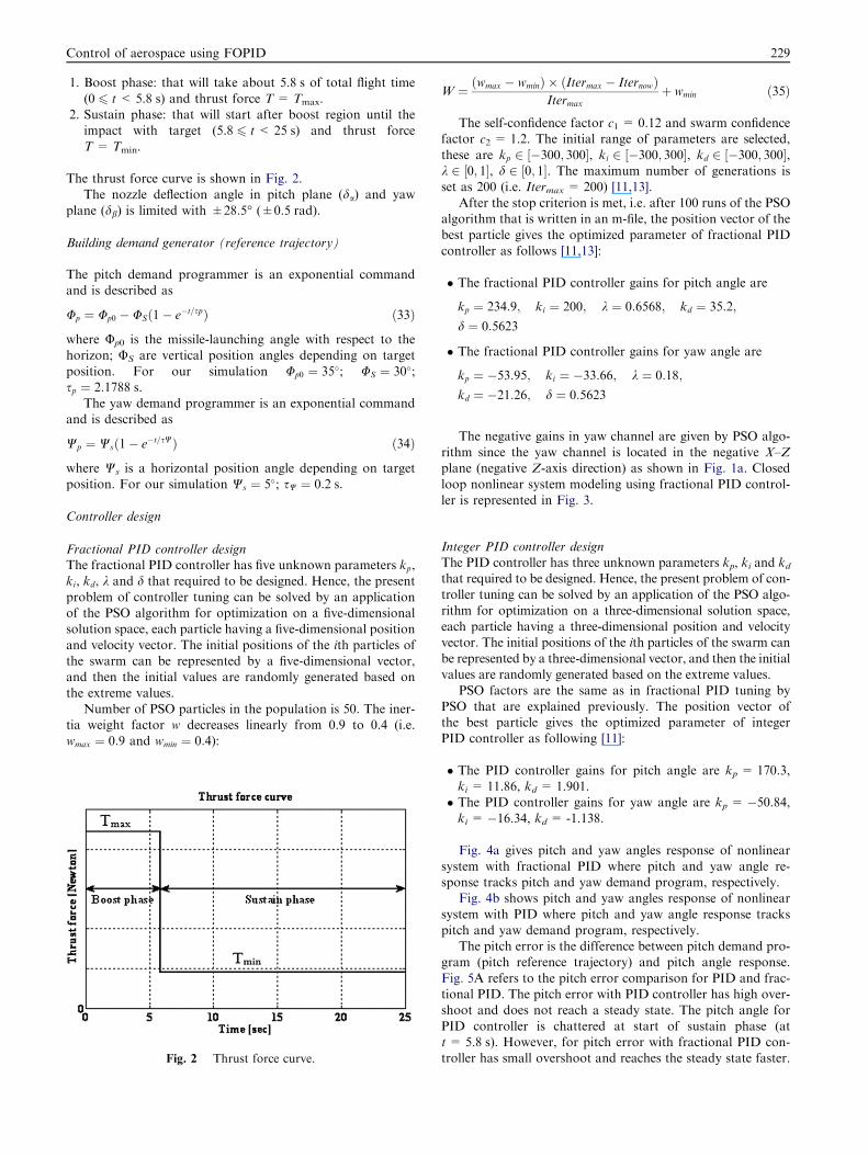
1. Boost phase: that will take about 5.8 s of total flight time

(0 6 t < 5.8 s) and thrust force T = Tmax.2. Sustain phase: that will start after boost region until the

impact with target (5.8 6 t< 25 s) and thrust force

T = Tmin.

The thrust force curve is shown in Fig. 2.The nozzle deflection angle in pitch plane (da) and yaw

plane (db) is limited with ±28.5� (±0.5 rad).

Building demand generator (reference trajectory)

The pitch demand programmer is an exponential commandand is described as

Up ¼ Up0 � USð1� e�t=spÞ ð33Þ

where Up0 is the missile-launching angle with respect to thehorizon; US are vertical position angles depending on target

position. For our simulation Up0 ¼ 35�; US ¼ 30�;sp ¼ 2:1788 s.

The yaw demand programmer is an exponential commandand is described as

Wp ¼ Wsð1� e�t=sWÞ ð34Þ

where Ws is a horizontal position angle depending on targetposition. For our simulation Ws ¼ 5�; sW ¼ 0:2 s.

Controller design

Fractional PID controller designThe fractional PID controller has five unknown parameters kp,ki, kd, k and d that required to be designed. Hence, the present

problem of controller tuning can be solved by an applicationof the PSO algorithm for optimization on a five-dimensionalsolution space, each particle having a five-dimensional position

and velocity vector. The initial positions of the ith particles ofthe swarm can be represented by a five-dimensional vector,and then the initial values are randomly generated based on

the extreme values.Number of PSO particles in the population is 50. The iner-

tia weight factor w decreases linearly from 0.9 to 0.4 (i.e.wmax ¼ 0:9 and wmin ¼ 0:4):

Fig. 2 Thrust force curve.

W ¼ ðwmax � wminÞ � ðItermax � IternowÞItermax

þ wmin ð35Þ

The self-confidence factor c1 = 0.12 and swarm confidencefactor c2 = 1.2. The initial range of parameters are selected,

these are kp 2 ½�300; 300�, ki 2 ½�300; 300�, kd 2 ½�300; 300�,k 2 ½0; 1�, d 2 ½0; 1�. The maximum number of generations isset as 200 (i.e. Itermax = 200) [11,13].

After the stop criterion is met, i.e. after 100 runs of the PSOalgorithm that is written in an m-file, the position vector of thebest particle gives the optimized parameter of fractional PID

controller as follows [11,13]:

� The fractional PID controller gains for pitch angle are

kp ¼ 234:9; ki ¼ 200; k ¼ 0:6568; kd ¼ 35:2;

d ¼ 0:5623

� The fractional PID controller gains for yaw angle are

kp ¼ �53:95; ki ¼ �33:66; k ¼ 0:18;

kd ¼ �21:26; d ¼ 0:5623

The negative gains in yaw channel are given by PSO algo-rithm since the yaw channel is located in the negative X–Zplane (negative Z-axis direction) as shown in Fig. 1a. Closed

loop nonlinear system modeling using fractional PID control-ler is represented in Fig. 3.

Integer PID controller designThe PID controller has three unknown parameters kp, ki and kdthat required to be designed. Hence, the present problem of con-troller tuning can be solved by an application of the PSO algo-

rithm for optimization on a three-dimensional solution space,each particle having a three-dimensional position and velocityvector. The initial positions of the ith particles of the swarm can

be represented by a three-dimensional vector, and then the initialvalues are randomly generated based on the extreme values.

PSO factors are the same as in fractional PID tuning by

PSO that are explained previously. The position vector ofthe best particle gives the optimized parameter of integerPID controller as following [11]:

� The PID controller gains for pitch angle are kp = 170.3,ki = 11.86, kd = 1.901.� The PID controller gains for yaw angle are kp = �50.84,ki = �16.34, kd = -1.138.

Fig. 4a gives pitch and yaw angles response of nonlinear

system with fractional PID where pitch and yaw angle re-sponse tracks pitch and yaw demand program, respectively.

Fig. 4b shows pitch and yaw angles response of nonlinear

system with PID where pitch and yaw angle response trackspitch and yaw demand program, respectively.

The pitch error is the difference between pitch demand pro-gram (pitch reference trajectory) and pitch angle response.

Fig. 5A refers to the pitch error comparison for PID and frac-tional PID. The pitch error with PID controller has high over-shoot and does not reach a steady state. The pitch angle for

PID controller is chattered at start of sustain phase (att= 5.8 s). However, for pitch error with fractional PID con-troller has small overshoot and reaches the steady state faster.

Fig. 3 Closed loop nonlinear system modeling using PIkDd controller.

Fig. 4a Pitch and yaw angles with fractional PID controller vs. time.

230 M.A.S. Aboelela et al.

The yaw error is the difference between yaw demand pro-gram (yaw reference trajectory) and yaw angle response. Theyaw error with PID and fractional PID is represented in

Fig. 5B. The yaw error with PID has high overshoot duringboost phase and sustain phase. However, for yaw error withfractional PID controller has small overshoot.

Conclusion

The design of PID controller is acceptable where it gives goodtracking with demand program but the design of fractionalPID controller gives more accurate tracking with demand pro-

gram. The design of fractional PID controllers gave the best

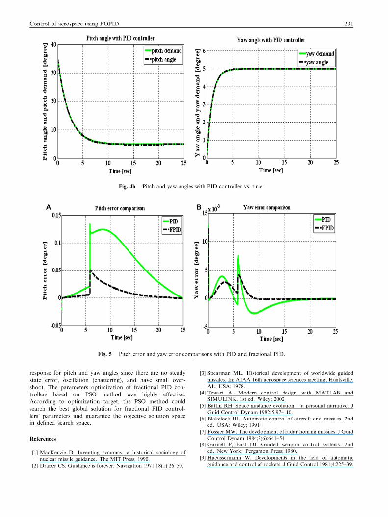
Fig. 4b Pitch and yaw angles with PID controller vs. time.

Fig. 5 Pitch error and yaw error comparisons with PID and fractional PID.

Control of aerospace using FOPID 231

response for pitch and yaw angles since there are no steadystate error, oscillation (chattering), and have small over-shoot. The parameters optimization of fractional PID con-

trollers based on PSO method was highly effective.According to optimization target, the PSO method couldsearch the best global solution for fractional PID control-

lers’ parameters and guarantee the objective solution spacein defined search space.

References

[1] MacKenzie D. Inventing accuracy: a historical sociology of

nuclear missile guidance. The MIT Press; 1990.

[2] Draper CS. Guidance is forever. Navigation 1971;18(1):26–50.

[3] Spearman ML. Historical development of worldwide guided

missiles. In: AIAA 16th aerospace sciences meeting, Huntsville,

AL, USA; 1978.

[4] Tewari A. Modern control design with MATLAB and

SIMULINK. 1st ed. Wiley; 2002.

[5] Battin RH. Space guidance evolution – a personal narrative. J

Guid Control Dynam 1982;5:97–110.

[6] Blakelock JH. Automatic control of aircraft and missiles. 2nd

ed. USA: Wiley; 1991.

[7] Fossier MW. The development of radar homing missiles. J Guid

Control Dynam 1984;7(6):641–51.

[8] Garnell P, East DJ. Guided weapon control systems. 2nd

ed. New York: Pergamon Press; 1980.

[9] Haeussermann W. Developments in the field of automatic

guidance and control of rockets. J Guid Control 1981;4:225–39.

232 M.A.S. Aboelela et al.

[10] Locke AS. Guidance (Principles of guided missile design

series). New Jersey: Van Nostrand/Macmillan; 1955.

[11] Maiti D, Acharya A, Chakraborty M, Konar A, Janarthanan R.

Tuning PID and FOPID controllers using the integral time

absolute error criterion. In: Proceedings of the fourth IEEE

international conference on information and automation for

sustainability, ICIAFS08, Colombo, Sir Lanka, December 11–

14, 2008.

[12] The Math Works Inc.. MATLAB 9.0 – User’s guide. Natick,

MA, USA: The Math Works Inc.; 2010.

[13] Siouris GM. Missile guidance and control systems. 1st ed. New

York, USA: Springer; 2004.

[14] Sung HA, Bhambhani V, Quan YC. Fractional-order integral

and derivative controller design for temperature profile control.

In: Chinese control and decision conference (CCDC), Utah

State University, USA; 2008.

[15] Westrum R. Sidewinder: creative missile development at China

Lake. Naval Institute Press; 1999.

[16] Yi Cao J, Gang Cao B. Design of fractional order controller

based on particle swarm optimization. Int J Control Automat

Syst 2006;4(6):775–81.