A methodology for national-scale flood risk assessment
33
Submitted October 2002 Substantially revised version submitted February 2003 A methodology for national-scale flood risk assessment Jim W Hall, BEng PhD CEng MICE Lecturer and Royal Academy of Engineering Post-Doctoral Research Fellow, Department of Civil Engineering, University of Bristol, Queen’s Building, University Walk, Bristol, BS8 1TR, UK Tel: 0117 928 9763, Fax: 0117 928 7783, Email: [email protected] Richard J Dawson, MEng Research Assistant, Department of Civil Engineering, University of Bristol, Queen’s Building, University Walk, Bristol, BS8 1TR, UK Tel: 0117 933 16785, Fax: 0117 928 7783, Email: [email protected] Paul B Sayers, BEng CEng MICE Group Manager, Engineering Systems and Management, HR Wallingford, Howbery Park, Wallingford, OX10 8BA, UK. Tel: 01491 822344, Fax: 01491 825539, Email: [email protected] Corina Rosu, PhD Marie Curie Fellow, HR Wallingford, Howbery Park, Wallingford, OX10 8BA, UK. Tel: 01491 835381, Fax: 01491 825539, Email: [email protected] John B Chatterton, BSc, PhD Principal, J. Chatterton Associates, 32 Windermere Rd, Moseley, Birmingham, B13 9JP, UK. Tel: 0121 449 7773, Email: [email protected] Robert Deakin, BSc GIS Group Manager, Halcrow Group Ltd, Burderop Park, Swindon, Wiltshire, SN4 0QD, UK Tel: 01793 812479, Fax: 01793 812089, Email: [email protected] Number of words: 6559 (187 synopsis) Number of tables: 2 Number of figures: 8
Transcript of A methodology for national-scale flood risk assessment

Submitted October 2002
Substantially revised version submitted February 2003
A methodology for national-scale flood risk assessment Jim W Hall, BEng PhD CEng MICE Lecturer and Royal Academy of Engineering Post-Doctoral Research Fellow, Department of Civil Engineering, University of Bristol, Queen’s Building, University Walk, Bristol, BS8 1TR, UK Tel: 0117 928 9763, Fax: 0117 928 7783, Email: [email protected] Richard J Dawson, MEng Research Assistant, Department of Civil Engineering, University of Bristol, Queen’s Building, University Walk, Bristol, BS8 1TR, UK Tel: 0117 933 16785, Fax: 0117 928 7783, Email: [email protected] Paul B Sayers, BEng CEng MICE Group Manager, Engineering Systems and Management, HR Wallingford, Howbery Park, Wallingford, OX10 8BA, UK. Tel: 01491 822344, Fax: 01491 825539, Email: [email protected] Corina Rosu, PhD Marie Curie Fellow, HR Wallingford, Howbery Park, Wallingford, OX10 8BA, UK. Tel: 01491 835381, Fax: 01491 825539, Email: [email protected] John B Chatterton, BSc, PhD Principal, J. Chatterton Associates, 32 Windermere Rd, Moseley, Birmingham, B13 9JP, UK. Tel: 0121 449 7773, Email: [email protected] Robert Deakin, BSc GIS Group Manager, Halcrow Group Ltd, Burderop Park, Swindon, Wiltshire, SN4 0QD, UK Tel: 01793 812479, Fax: 01793 812089, Email: [email protected] Number of words: 6559 (187 synopsis) Number of tables: 2 Number of figures: 8
Synopsis
Risk analysis provides a rational basis for flood management decision-making at a national
scale, as well as regionally and locally. National-scale flood risk assessment can provide
consistent information to support the development of flood management policy, allocation of
resources and monitoring the performance of flood mitigation activities. However, national-
scale risk assessment presents particular challenges in terms of data acquisition and
manipulation, numerical computation and presentation of results. A methodology that
addresses these difficulties through appropriate approximations has been developed and
applied in England and Wales. The methodology represents the processes of fluvial and
coastal flooding over linear flood defence systems in sufficient detail to test alternative policy
options for investment in flood management. Flood outlines and depths are generated, in the
absence of a consistent national topographic and water level data set, using a rapid parametric
inundation routine. Potential economic and social impacts of flooding are assessed using
national databases of floodplain properties and demography. A case study of the river Parrett
catchment and adjoining sea defences in Bridgwater Bay in England demonstrates the
application of the method and presentation of results in a Geographical Information System.
1 INTRODUCTION
Over 5% of the UK population live in the 12,200km2 that is at risk from flooding by rivers
and the sea1. These people and their property are protected by 34,000km of flood defences.
Serious flooding in 1998 and 2000 demonstrated the need for improved management of flood
defences2,3,4,5. Recently the UK government has allocated more resources for improving flood
and coastal defence standards6. Flood risk assessment is required to support the appraisal of
policy options, allocation of resources and monitoring performance of substantial government
investment in flood management.
The amount of resource, in terms of data acquisition and analysis, that is committed to a risk
assessment should reflect the nature of the decision(s) that the assessment seeks to inform.
Flood management decisions take place at a number of levels, ranging from national policy
decisions to planning decisions in catchments and coastal cells and local design and
operational decisions. A hierarchy of flood risk assessment methods is therefore currently
under development to support a range of flood management decisions (Table 1), building on
previous tiered frameworks7,8,9.
2
This paper addresses the highest level in the hierarchy of flood management decisions, with
the aim of supporting national-scale flood defence policy making. National-scale risk
assessment is by no means straightforward, because of the need to assemble national datasets
and then carry out and verify very large numbers of calculations. The first assessment on this
scale in the UK was published by HR Wallingford in 20001 and provided an estimate of
potential damage from flooding and coastal erosion in England and Wales. The 2000 study
made use of nationally available flood outlines (the so-called Indicative Floodplain Maps) and
datasets on the domestic and industrial properties in floodplains. However, at the time a
national database of flood defences and their condition was not accessible, so the analysis
necessarily made significant simplifications regarding the influence of defences on flood risk,
taking no account of the standard of protection and condition of defences.
In 2002 the Environment Agency introduced a National Flood and Coastal Defence Database
(NFCDD), which for the first time provides in a digital database an inventory of flood defence
structures and their overall condition. Whilst the information held in NFCDD and other
nationally available datasets is still limited, it has paved the way for the first national
assessment of flood risk that incorporates probabilistic analysis of individual defence
structures as well as the flood defence systems they create. This also means that possible
changes in the performance of defences infrastructure under hydraulic loading (for example
due to deterioration in condition, improvement in standard of protection or change in loading)
can be evaluated. The risk assessment methodology therefore provides a tool for exploring the
impact of future flood management policy and scenarios of climate change. Use of a national
digital database is also attractive in that it enables changes in data to be automatically
reflected within the assessment of flood risk. The objective of this paper is to describe this
new national-scale flood risk assessment methodology.
2 OVERVIEW OF THE METHODOLOGY
Flood risk is conventionally defined as the product of the probability of flooding and the
consequential damage and is often quoted in terms of an expected annual damage, which is
sometimes referred to as the ‘annual average damage’. For a national assessment of flood risk,
expected annual damage must be aggregated over all floodplains in the country. An overview
of the methodology by which this can be achieved is given in and described in
outline below.
Figure 1
3

The most significant constraint on a national-scale flood risk assessment methodology is the
availability of data. The methodology presented here has been developed to make use of the
following national GIS datasets and no other site-specific information:
1. Indicative Floodplain Maps (IFMs) are the only nationally available information on the
potential extent of flood inundation. The IFMs are outlines of the area that could
potentially be flooded in the absence of defences in a 1:100 year return period flood for
fluvial floodplains and a 1:200 year return period flood for coastal floodplains.
2. 1:50,000 maps with 5m contours. The methodology has been developed in the absence of
a national topographic dataset of reasonable accuracy. Topographic information at 5m
contour accuracy has only been used to classify floodplain types as it is not sufficiently
accurate to estimate flood depths.
3. National map of the centreline of all watercourses.
4. National Flood and Coastal Defence Database provides national dataset of defence
location, type and condition. Crucially however, information on crest level and crest width
are not mandatory and, therefore, are not available nationally. The methodology has been
developed in the absence of quantitative information on the distribution of water levels
and wave loads.
5. National database of locations of residential and business properties.
In the absence of more detailed information on flood extent, in the current methodology the
Indicative Floodplain is adopted as the maximum extent of flooding and is further sub-divided
into Impact Zones, not greater than 1km × 1km. Each flood Impact Zone is associated with a
system of flood defences which, if one or more of them were to fail, would result in some
inundation of that zone.
The probability of failure of a flood defence system can be estimated using the methods of
structural reliability analysis10,11. However, to apply these methods requires (i) probability
distributions for the hydraulic loads and the parameters describing defence response and (ii)
analytical or numerical expressions for each failure mode. Unfortunately the only available
information on the relationship between flood water level and crest level, clearly crucial for
flood risk analysis, is the so-called Standard of Protection (SOP), which is an assessment of
the return period at which the defence will significantly be overtopped. In the current
methodology the SOP is used to determine the frequency with which a defence is expected to
be overtopped. It is also possible to estimate the frequency with which the defence will
4
experience loads some factor times the SOP, for example loads twice or half as severe as the
SOP. In this way a probability distribution of load relative to SOP is constructed.
Next, flood defence failure is addressed by estimating the probability of failure of each
defence section in a given load (relative to SOP) for a range of load conditions. Generic
versions of these probability distributions of defence failure, given load, have been
established for a range of defence types for two failure mechanisms, overtopping and
breaching.
Having estimated the probability of failure of individual sections of defence, the probabilities
of failure of combinations of defences in a system are calculated. For each failure scenario an
approximate flood outline is generated using parametric routines. These routines estimate
discharge through or over the defence and inundation characteristics of the floodplain. In the
absence of water level and topographic data, estimation of flood depth has been based on
statistical data. This data was assembled from real and simulated floods in a range of
floodplain types and floods of differing return periods. Economic risk is calculated based on
damage to properties and agricultural land use within the flooded area. Insight into the
population at risk is obtained from census data and a measure of the social harm of flooding is
obtained from Social Flood Vulnerability Indices12.
3 FLOOD DEFENCE SYSTEMS RELIABILITY ANALYSIS
Consider a flood defence system with n defence sections, labelled d1, d2,…, dn. Each defence
section has independent and usually a different resistance to flood loading. There are m flood
Impact Zones, labelled z1, z2,…, zm, within the Indicative Floodplain. The remaining perimeter
of the floodplain is high ground. A simple example of such a system is shown in Figure 2.
Failure of one or more of the defences by overtopping or breaching will inundate one or more,
but not necessarily all, of the flood Impact Zones. For each flood Impact Zone, the probability
of every scenario of failure that may cause or influence flooding in that zone is required.
Consider an Impact Zone protected by two defences d1 and d2. Label the failure of defence di
as event Di and non-failure as event iD
2D
. In this case there are three failed scenarios of
defence system failure. The first scenario is where both defences fail. In more formal terms
this can be expressed as event , where the symbol ∩ signifies a joint combination of
events i.e. signifies “Event D
1D ∩
21 DD ∩ 1 and event D2 occur”. Two more failed scenarios must
5

be considered, 21 DD ∩ , 21 DD ∩ , and scenario where neither of the defences fail (a non-
failed scenario), 21 DD ∩ .
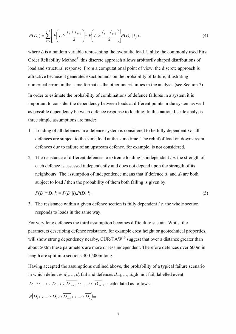
)|( dxxDi
)|( dllDi
The probability of failure of a defence is a function of the probability of an extreme load
(river water level or marine storm) and the defence resistance to that load. In the absence of
information on the frequency of extreme loads, a factor x times the SOP has been adopted as a
proxy for load. Thus if the SOP is 1:100 years, then a load with x = 0.5 corresponds to a 1:50
year return period event. Note that there is not a linear relationship between x and the physical
loading variable(s) e.g. water level. The annual probability P(X ≥ x) of at least one load event
X with severity greater than or equal to x at a defence with Standard of Protection SOP can be
approximated as:
P(X ≥ x) = SOP.1
x. (1)
provided x.SOP > 5.
Each defence section di is assigned, on the basis of its type and condition, a conditional
probability of failure event Di for a given load x, P(Di|x), for a range of values of x. In
reliability analysis a conditional probability distribution of this type is referred to as a
‘fragility curve’13,14. Typical fragility curves are illustrated in Figure 3. By integration over all
loading conditions the fragility curve can be combined with the loading distribution to
generate an unconditional probability of defence failure, P(Di):
∫∞
=0
)()( PxpDP i (2)
where p(x) is the probability density function of the load x, which is derived from Equation 1
as explained below. The product x.SOP is a measure of the severity of the hydraulic load, so it
is replaced by the symbol l, in which case:
∫∞
=0
)()( PlpDP i (3)
and P(Di|l) can be obtained from the fragility curve by reading off at x = l/SOP. If Equation 1
is to be used to estimate p(l) then P(Di|l) should be close to zero where l is outside the range
of applicability of Equation 1. For the purpose of the current analysis the fragility curve is
defined in discrete terms at q levels of l: l1,…, lq, enabling Equation 3 to be re-written as:
6
)|(22
)(1
2
11ji
q
j
jjjji lDP
llLP
llLPDP ∑
−
=
−+
+>−
+≥= . (4)
where L is a random variable representing the hydraulic load. Unlike the commonly used First
Order Reliability Method11 this discrete approach allows arbitrarily shaped distributions of
load and structural response. From a computational point of view, the discrete approach is
attractive because it generates exact bounds on the probability of failure, illustrating
numerical errors in the same format as the other uncertainties in the analysis (see Section 7).
In order to estimate the probability of combinations of defence failures in a system it is
important to consider the dependency between loads at different points in the system as well
as possible dependency between defence response to loading. In this national-scale analysis
three simple assumptions are made:
1. Loading of all defences in a defence system is considered to be fully dependent i.e. all
defences are subject to the same load at the same time. The relief of load on downstream
defences due to failure of an upstream defence, for example, is not considered.
2. The resistance of different defences to extreme loading is independent i.e. the strength of
each defence is assessed independently and does not depend upon the strength of its
neighbours. The assumption of independence means that if defence d1 and d2 are both
subject to load l then the probability of them both failing is given by:
P(D1∩D2|l) = P(D1|l).P(D2|l). (5)
3. The resistance within a given defence section is fully dependent i.e. the whole section
responds to loads in the same way.
For very long defences the third assumption becomes difficult to sustain. Whilst the
parameters describing defence resistance, for example crest height or geotechnical properties,
will show strong dependency nearby, CUR/TAW10 suggest that over a distance greater than
about 500m these parameters are more or less independent. Therefore defences over 600m in
length are split into sections 300-500m long.
Having accepted the assumptions outlined above, the probability of a typical failure scenario
in which defences d1,…, dr fail and defences dr+1,…, dn do not fail, labelled event
nrr DDDD ∩∩∩∩∩ + ..... 11 , is calculated as follows:
( )=∩∩∩∩∩ + nrr DDDDP ...... 11
7

)|()...|().|()...|(22 1
1
21
11jnjrjr
q
jj
jjjj lDPlDPlDPlDPll
LPll
LP +
−
=
−+∑
+≥−
+≥ (6)
To understand the impact of defence failure it is also important to establish the mode of
failure, be it breach or overtopping. The impacts of overtopping and breaching failure modes
can be quite different, so denote failure of defence di by overtopping as Di,OT and its failure by
breaching as Di,B. Non-failures are labelled OTiD , and BiD , respectively. Breaching and
overtopping are not independent failure mechanisms. Indeed overtopping is one of the
common initiating mechanisms of a breach. This dependency is accounted for by first
considering the probability of failure by overtopping given a particular load l, P(Di,OT|l) and
then the probability of breaching, with or without overtopping, again in load l, labelled
( )lDDP OTiBi ,| ,, and ( )lDDP OTiBi ,| ,, respectively. The probability of breaching in load l,
( )lDP Bi |, , is therefore
( ) ( ) ( ) ( ) ( )lDPlDDPlDPlDDPlDP OTiOTiBiOTiOTiBiBi |.,||.,|| ,,,,,,, += (7)
and we know that ( ) ( )lDPlDP OTiOTi |1| ,, −= , so
( ) ( ) ( ) ( ) ( )[ ]lDPlDDPlDPlDDPlDP OTiOTiBiOTiOTiBiBi |1,||.,|| ,,,,,,, −+= . (8)
To evaluate Equation 8 requires three fragility curves: (i) overtopping, ( )xDP OTi |, , (ii)
breaching given overtopping, ( )xDDP OTiBi ,| ,, and (iii) breaching given no overtopping,
( )xDDP OTiBi ,| ,, . Considering one typical scenario, where the first defence is overtopped, the
second defence is breached and the remaining defences, d3,…, dn, do not fail
i.e. nBOT DDDD ∩∩∩∩ ...3,2,1 , Equation 6 (setting r = 2) becomes:
( )=∩∩∩∩ + nrBOT DDDDP ...1,2,1
)|()...|().|().|(22 3,2
1
2,1
11jnjjB
q
jjOT
jjjj lDPlDPlDPlDPll
LPll
LP∑−
=
−+
+≥−
+≥ (9)
where is obtained from Equation 8. )|( ,2 jB lDP
For each defence there are three states that are of interest: overtopped, breached and not
failed. For an Impact Zone protected by n defences there are therefore 3n system states whose
probabilities are to be estimated. For a large system, the analysis of such a large number of
8
scenarios may require an excessive amount of computer processing time. However, high order
scenarios, i.e. scenarios in which a large number of defences in a system all fail, make a small
contribution to the total probability of failure so can be neglected. The error due to this
approximation can be calculated exactly provided the probability of non failure for the whole
system ( )nDDDP ∩∩∩ ...21 is also calculated. Suppose that in a system with n defence
sections, the probabilities of all scenarios with between zero and five failures have been
calculated. There will be
∑= −
=5
0 )!(!!
i inint (10)
such scenarios, the probability of each of which is labelled Pk, k = 1,…, r. The error E from
neglecting higher order scenarios is given by
∑=
−=t
kkPE
11 (11)
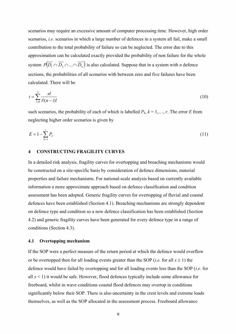
4 CONSTRUCTING FRAGILITY CURVES
In a detailed risk analysis, fragility curves for overtopping and breaching mechanisms would
be constructed on a site-specific basis by consideration of defence dimensions, material
properties and failure mechanisms. For national-scale analysis based on currently available
information a more approximate approach based on defence classification and condition
assessment has been adopted. Generic fragility curves for overtopping of fluvial and coastal
defences have been established (Section 4.1). Breaching mechanisms are strongly dependent
on defence type and condition so a new defence classification has been established (Section
4.2) and generic fragility curves have been generated for every defence type in a range of
conditions (Section 4.3).
4.1 Overtopping mechanism
If the SOP were a perfect measure of the return period at which the defence would overflow
or be overtopped then for all loading events greater than the SOP (i.e. for all x ≥ 1) the
defence would have failed by overtopping and for all loading events less than the SOP (i.e. for
all x < 1) it would be safe. However, flood defences typically include some allowance for
freeboard, whilst in wave conditions coastal flood defences may overtop in conditions
significantly below their SOP. There is also uncertainty in the crest levels and extreme loads
themselves, as well as the SOP allocated in the assessment process. Freeboard allowance
9
cannot be assumed to be nationally uniform, because of different local conventions and
assumed rates of settlement. The fragility curves shown in Figure 3 have therefore been
adopted. The curve shows a significant chance of overtopping at x < 1, especially for coastal
defences, but the defence is not guaranteed to overtop at x > 1. Uncertainty is reflected
through the use of upper and lower bounds on the conditional failure probability for a given
load, x, as described in Section 7. Evidence from floods of known severity overtopping
defences of known SOP, primarily from records of the autumn/winter floods of 200015, have
been used to verify points on this curve.
4.2 Defence classification
In England and Wales the Environment Agency classifies every flood defence based on the
individual defence components (for example inward slope, crest and outward slope) and their
composition (for example turf or concrete)16. This leads to a classification in which sub-
divisions have little bearing on the proneness to failure, whilst important characteristics such
as crest width and level can go unrecorded.
For the purpose of national-scale risk analysis a simple new classification has been developed,
focussing on those salient characteristics of a defence cross-section that influence its
resistance to extreme loads. An algorithm has been established that gives a direct mapping
from the classification used by the Environment Agency to the new classification introduced
here.
At the high level in the classification are seven defence types that show significantly different
behaviour (Figure 4). The next level within the hierarchy considers the degree of protection
offered by the defence. A wider defence will provide more protection than a narrow defence,
as will a defence that is protected on its front slope, crest and rear slope, compared to one
without protection8. The next level of classification considers the properties of individual
components.
4.3 Breaching mechanism
The probability of breaching in a storm of given severity is influenced by the type of defence
and its condition. As suggested in Section 3, it is also strongly influenced by presence or
absence of defence overtopping. Therefore a family of fragility curves have been developed
including each defence classification, condition grade and overtopping/non-overtopping
cases. The fragility curves were are developed using a similar technique to that proposed by
10
the USACE17 in which critical points on the curve are fixed by a combination of expert
judgement and analysis, with a straight line between them.
The only nationally available information on defence condition is a visual assessment that
grades each defence from Grade 1 (“very good”) to Grade 5 (“very poor”). The Environment
Agency’s Condition Assessment Manual18 provides benchmark photographs of the main types
of defence in all five conditions. Grade 5 nominally represents a defence in an effectively
failed condition. However, the photographs in the Condition Assessment Manual indicate that
some of these defences would afford some resistance against breaching, at least in loads
where x < 1, so a fragility curve has been established based on assessment of this residual
resistance. Unfortunately field evidence of defence breaching in loads of known severity for
defences in known pre-storm condition is very scarce indeed. Verification of the fragility
curves has therefore been based primarily on published values of the resistance of defence
materials to overtopping8,10,19.
5 FLOOD INUNDATION
Having estimated the probability of every scenario of defence system failure, the
consequences of flooding are established by first estimating flood depths (this Section) and
then estimating damage (Section 6). Flood depth estimation is based on volumetric analysis
that employs a series of simple approximations. Further justification for these approximations
is provided in HR Wallingford Report SR60320. The inundation calculations outlined below
are conducted for every failure scenario of breaching and/or overtopping and at every discrete
level of loading. The purpose of the inundation method is to estimate the flood depth in a
specified scenario, irrespective of the probability of that scenario occurring. The depth
estimates are then weighted according to the probability of each failure scenario (Section 5.5).
5.1 Overtopping flood volumes – fluvial flood plains
In the case of overtopping of a fluvial defence, the flow of water over or through the defence
is similar to the flow over a rectangular, broad-crested weir and, therefore, the peak discharge
qp (m3/s/m) is given by21:
5.1max71.1 bhq p = (12)
where b is flow width (in metres), which is taken as equal to the defence length, and hmax is
the maximum head (in metres) over the defence crest, which is approximated by20:
11
2max 05.0 xh = (13)
As previously, x is the ratio of the return period of the event under consideration to the SOP
of the defence, and is allowed to take any value between 0 and 3. An upper limit to the ratio x
has been imposed to reflect the natural limit to hmax over any single defence. Above this limit,
overtopping of upstream defences, a process that is not explicitly represented in the
methodology, is likely to limit the continued increase in hmax with increasing load. The flood
volume (m3) from failure of defence section i, Vi, is estimated as:
Vi = 0.5qpTf(x) (14)
where Tf(x) is duration of flow across the defence (in seconds), given as a function of the
form20:
Tf(x) = (15) 5.025.0 BxA
where A is the catchment area (km2) and the coefficient B is obtained from Table 2, yielding
Tf in hours. In Equation 14 both the duration, Tf, of the flow across the defence and the
maximum depth, hmax, of flow over defence depend on the ratio x. Therefore, both duration
and water depth will increase as the ratio x increases.
5.2 Overtopping flood volumes – coastal floodplains
Coastal overtopping is estimated from:
Vi = qbTc(x) (16)
where b is the length of the defence overtopped (in metres), Tc(x) is the effective duration of
the overtopping event converted into seconds and the overtopping q (m3/m/s) is approximated
from20:
5.105.0 xq = (17)
The rate q = 0.05 m3/m/s at x = 1 is taken as the definition of significant overtopping in an
event equal to the SOP, and the power 1.5 has been extracted by fitting to the results of
typical overtopping analysis19. The duration of coastal storms is strongly influenced by the
rise and fall of the tide and can be approximated (in hours) as:
sc TxxT =)( (18)
where Ts = 3 hours, which is the typical effective duration of an overtopping event during a
storm equal to the SOP. In the limit, i.e. when x = 3, (for example, in a 1:600 year return
12
period event and a defence with an SOP of 1:200 years) this implies a maximum duration of a
coastal overtopping event of 9 hours. In practice this will depend on the relative magnitude of
the astronomical tide and the surge residual but in the absence of strong evidence to the
contrary the adopted value has been found to be a good first approximation.
5.3 Breach flood volumes – fluvial and coastal floodplains
Overtopping is assumed to occur over the entire defence length Sd, whereas the breach width
bB is estimated as a function of x20:
dB xSb 05.0= , (19) dB Sb ≤
Whilst there is little information on the breaching process, observational evidence from the
Autumn 2000 Flood records (for example, in Lewes where river walls with SOP of 30-50yrs
breached along 33m in three sections during a 70-100 year return period event) has been used
to support Equation 19. The flood volume is then estimated from Equation 14, using Tf(x)
values from Equation 15 for fluvial defences, and substituting Tc(x) (Equation 18) for Tf(x) in
the case of coastal defences. It is assumed that the duration of flow through a breach will be
the same as the overtopping duration for a storm of given severity. In both cases the
maximum head, hmax, over the breach is assumed to be given by20:
5.0max 5.0 xh = (20)
i.e. the depth of flow is taken as 0.5m when x=1.
5.4 Flood extent
The flood extent is obtained by spreading the flood volume assuming an average flood depth
and outline shape. First a uniform flood depth of 0.2m is assumed together with either a semi-
circular or trapezoidal outline shape constrained by the Indicative Floodplain to establish the
limits of flooding for a given volume. Note that this depth is only used to estimate the flood
outline and is not directly used in the damage assessment.
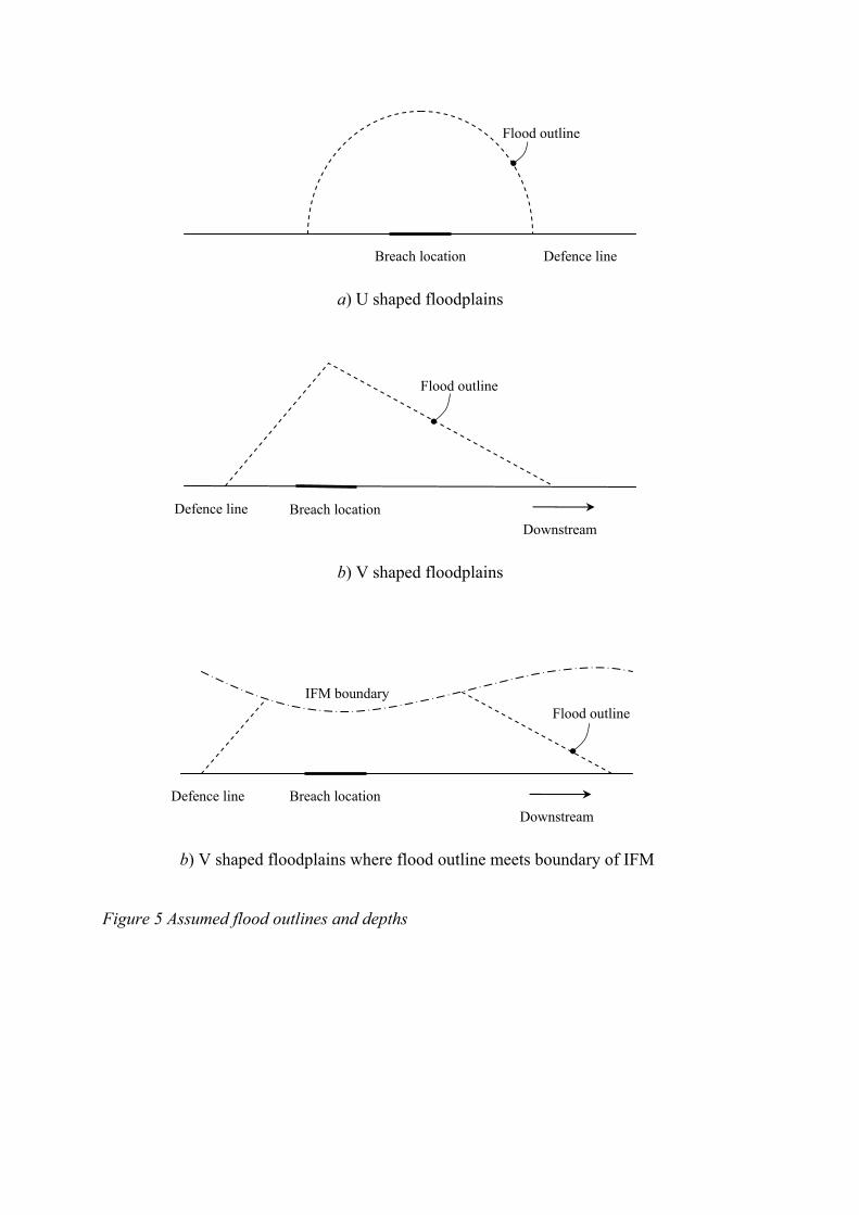
To determine the outline shape, the floodplain is classified using a 1:50,000 digital terrain
model and the Indicative Floodplain Maps (IFMs) as U-shaped for flat floodplains, V-shaped
for steeply sloping narrow floodplains, or W-shaped for compound floodplains in which
depths flood depths increase from the river and then reduce22. U-shaped and coastal
floodplains are assumed to have a semi-circular flood outline centred at the point of failure,
with equal up and downstream flooding ( a). V-shaped floodplains are assigned an Figure 5
13
asymmetrical triangular outline, with a greater downstream flooding ( b). For all
floodplains, when the flood outline reaches the extent of the Indicative Floodplain it is
elongated upstream and downstream rather than allowing it to cross the floodplain boundary
( c).
Figure 5
Figure 5
The analysis proceeds by considering in turn every Impact Zone in the floodplain ( )
and analysing only those defences whose failure could have some influence on flooding
within that zone. This enables defences that contribute to flooding within an Impact Zone to
be identified and provides a mechanism for significantly reducing the number of defence
failure scenarios that need to be considered for each Impact Zone.
Figure 2
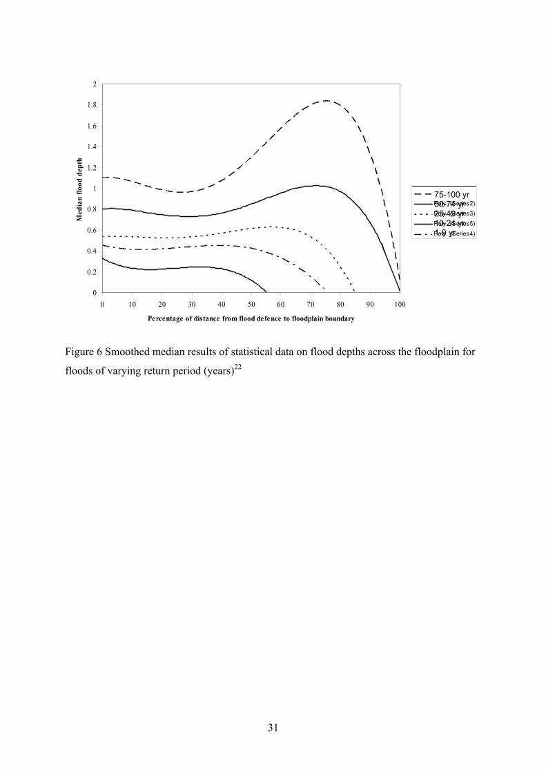
5.5 Flood depth
In the absence of topography and quantitative water level data, flood depth has been
calculated using a statistical representation of typical flood depths that may be expected, in
the absence of defences, in a range of storm events. This statistical model had been developed
previously by Middlesex University22 through analysis of 70 flood scenarios (real and
simulated). Based on these results, estimates of flood depth at points across the floodplain in
floods of a range of severities was generated ( ). These data were used to estimate
flood depth at points between a failed defence and the floodplain boundary, in events of a
given severity. The Middlesex data related to flood depths immediately behind the failed
defence so were further modified to estimate flood depths up and down-stream (or along the
coast) from the failure. The depth is assumed to decrease linearly, by factor e, with distance
upstream and downstream of the failure location, where e = 1 at the failed defence and e = 0
at the predicted limit of the flood outline. In the case of multiple defence failures resulting in
the flood outlines overlapping, the factor e is aggregated to a maximum of 1.
Figure 6
If a given point in the floodplain is predicted to be inundated in k different defence failure
scenarios, each of which results in a flood depth yj, j = 1,…, k, with corresponding probability
Pj then the probability of the flood depth Y exceeding some value y is given by:
∑≥
=≥yy
jj
PyYP )( (21)
6 ANALYSIS FOR FLOOD DAMAGE
The probability distribution of flood depth (Equation 20) was calculated at the centroid of
each Impact Zone and assumed to apply to the whole of the Impact Zone.
14
6.1 Economic damage
The numbers of domestic and commercial properties in each Impact Zone were extracted
from nationally available databases of economic damage values at given flood depths. For a
given Impact Zone the expected annual damage R is given by
∫=max
0)()(
ydyyDypR (22)
where ymax is the greatest flood depth from all failure scenarios, p(y) is the probability density
function for flood depth, which can be obtained from Equation 20, and D(y) is the damage in
the Impact Zone in a flood of depth y metres. The total expected annual damage for a
catchment or nationally is obtained by summing the expected annual damages for each Impact
Zone within the required area.
6.2 Social impacts
The population at risk was estimated from the number of inhabitants within an Impact Zone
using 2001 census data. The Social Flood Vulnerability Indices (SFVI)12 were used to
identify communities vulnerable to the impacts of flooding. Social vulnerability is ranked
from “very low” to “very high” and is based on a weighting of the number of lone parents, the
population over 75 years old, the long term sick, non-homeowners, unemployed, non-car
owners and overcrowding, obtained from census returns. The risk of social impact is obtained
as a product of probability of flooding to a given depth and the SFVI, providing a
comparative measure for use in policy analysis.
7 HANDLING UNCERTAINTY
Each of the stages in the methodology outlined above is prone to uncertainty because of the
approximations in the methodology and the great variability in the quality of data available
for national-scale analysis. At a national scale many local errors will cancel each other out.
However, it has been necessary to estimate risk at a fairly detailed local scale before
aggregating risk nationally. These local assessments provide a useful starting point or cross-
check for more detailed analysis, but are rather approximate so have the potential to be quite
misleading, particularly if quoted to an inappropriate precision.
A simple but explicit method of representing uncertainty has been adopted at each stage in the
analysis and carried through to all results. Uncertainty is represented by dealing with lower
and upper bounds on each of the most uncertain quantities. For example the uncertainty in the
15
fragility curves is addressed by representing these curves as upper and lower bound on the
curves shown in Figure 3. Thus risk estimates are presented as upper and lower bounds. These
bounds have been elicited from experts as the credible limits between which they expect the
actual value to lie. No calibration of expert judgement has been applied but the judgement of
several experts has been pooled in the analysis in order to address bias and over-confidence in
expert judgements. No assumption about the distribution of risk between these bounds is
implied, though in the absence of further information the best estimate will lie at the
midpoint. This best estimate should only be quoted on a whole catchment or national basis. At
a more local scale the wide bounds on risk estimates will provide a motive for further data
collection and analysis.
8 EXAMPLE IMPLEMENTATION
The flood risk assessment methodology was first tested on the Parrett catchment in the South
West of England, a system of sufficient complexity to evaluate the robustness of the
methodology, before proceeding to the full national assessment. The lower reaches of the
Parrett include a network of drainage channels, whereas the upper reaches are quite steep. The
fluvial defences adjoin short sections of sea defence in Bridgwater Bay. To enable
comparison with a previous study1, inflation-adjusted depth-damage data from 199023 rather
than the most recent data24 were used in the test implementation.
Establishing the defence system involved merging geographically indexed data on flood
defences from the NFCDD with data on the centreline of all watercourses, held by CEH
Wallingford. A continuous defence line on both banks of every watercourse and along all
coastlines fronting the floodplain was generated. Significant lengths of river were not reported
in the NFCDD as having a defence, in which case it was assumed that there was no raised
defence. Large numbers of very small isolated patches of floodplain were located near the
edge of the floodplain due to the rasterization of the IFM. These very small sections of
floodplain were merged with the bulk of the floodplain as they contributed insignificantly to
the overall risk but added substantial computational burden.
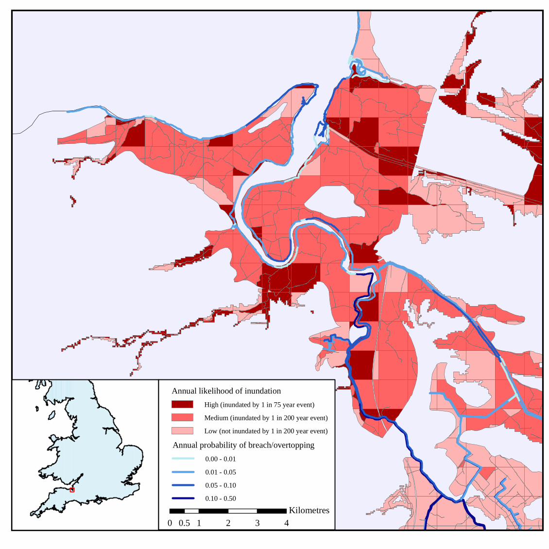
The two main outputs for the analysis20, which were geographically indexed in a
Geographical Information System (GIS), were the risk in each Impact Zone and the average
contribution to this risk from each defence in the flood defence system. Figure 7 shows the
output from the economic risk assessment. The total expected annual damage for the Parrett
catchment was calculated as £1.4-£2.1million. This compares with the only previous analysis1
16

which provided a single estimate of the total risk of £2.7 million. In the close-up of the Parrett
estuary shown in the defence line has been coloured to represent the probability of
failure of each defence, with the darker shade signifying a higher failure probability. The
contribution to flood risk from each defence can also be extracted and plotted geographically.
Figure 8
As well as providing an assessment of present risk, the methodology can be used to test future
flooding scenarios and policy options, provided these can be resolved using the parameters of
the methodology. For example, to illustrate the potential impact of climate change, the SOP of
all defences was reduced by 20% (this reflects to an increase in water levels as a result of
climate change). Therefore a defence that provided protection to a 1:200 year SOP effectively
reduced to a 1:160 year SOP. In this climate change scenario the total economic risk increased
to an expected annual damage of £1.8-£2.7million.
The influence of repairing defences in poor condition can be assessed by altering the
condition grade of defences. All defences with condition grade below 2 (“good”) were raised
to grade 2, reducing the total economic risk to an expected annual damage of £1.3-£2.0
million. This decrease is not particularly dramatic because most of the defences on the Parrett
are already condition grade 2 or 3, and because the resistance to failure of a defence with
condition grade 3 is not much worse than one with condition grade 2. The decrease in annual
average risk can be weighed against the estimated cost of repairing the defences.
Other queries that can be made on the output data include:
1. risk contribution from defences aggregated by condition grade;
2. risks contribution from defences aggregated by SOP;
3. risks contribution from floods of varying severity;
4. number of houses at risk of flooding to a given depth with a given probability. For
example, in the Parrett catchment, between 2335 and 2704 residential properties (out of a
possible 15668) and from 492 to 601 non residential properties (out of a possible 1605)
are expected to be flooded to a depth of 0.2m or greater in a 1:100 year flood.
9 LIMITATIONS AND DIRECTIONS FOR MORE DETAILED ANALYSIS
As has been stressed throughout this paper, national assessment of flood risk is severely
limited by availability of data and also to some extent by computational constraints. The
method has been designed to give an unbiased aggregate measure of risk on a national basis
17
and cannot be expected to be consistently accurate for every locality. Key limitations that the
reader should note are as follows:
1. The frequency of extreme fluvial flows or marine storms has not been assessed directly.
The factor x times SOP has been used as a proxy for load.
2. Probabilistic analysis of defence resistance using fragility curves is based on a simple
defence classification and generic fragility curves that do not take explicit account of
defence geometry and other key parameters that determine defence resistance.
3. The current quality of information relating to defence location, condition and SOP within
the NFCDD is highly variable.
4. The flood spreading routine is based on volumetric concepts but does not include any
hydrodynamic modelling and is based on a simple characterisation of floodplain
morphology and approximate flood outlines in the IFM.
5. Flood depths are based on statistical analysis of real and simulated data and do not take
account of local topography.
Whilst these approximations are appropriate for national-scale risk assessment, site specific
decision-making, for example for Catchment Flood Management Planning or scheme design,
will require more detailed data collection and analysis. The following aspects must be given
more attention in more detailed analysis:
1. Statistical analysis of hydrology, and joint probability loading conditions for sea defences,
including spatial dependency and antecedent conditions in both cases.
2. Quantified analysis of multiple defence failure modes making use of site-specific
measurements.
3. Analysis of the dependency between defence strength parameters within defence sections
and between neighbouring sections.
4. Hydrodynamic modelling for flood depth and extent using high resolution topographic
information.
5. Consideration of the influence on flooding of groundwater and local runoff.
6. More detailed analysis of tangible and intangible impacts of flooding, including disruption
to transportation systems.
18
7. Analysis of the influence of non-structural flood mitigation measures such as flood
warning.
Furthermore, when more detailed information is available in an appropriate format this can
also contribute to national-scale analysis. More detailed analysis will also contribute to
verification of the national-scale method.
10 CONCLUSIONS
The methodology outlined in this paper represents a significant advance on the only previous
national appraisal of flood risk and is a step towards fully probabilistic, process-based
assessment of national flood risk from fluvial and coastal sources. The methodology uses only
nationally available datasets in England and Wales. It has been tested on the Parrett catchment
in South-West England and has now been applied to all of England and Wales. The risk
assessment methodology is based on analysis of systems of linear flood defences, taking into
account the defence Standard of Protection, type and condition grade.
The methodology provides an estimate of economic risk for zones within the floodplain,
which can be aggregated to a regional and national scale. Use of Social Flood Vulnerability
Indices gives a measure of the potential social impact of flooding. The methodology also
identifies the contribution to risk of individual defence sections. It can be used in national
policy analysis by testing scenarios of changed flood frequency, investment in flood defences
or floodplain occupancy. It can also form the starting point for more detailed catchment and
local-scale analysis.
11 ACKNOWLEDGEMENTS
The research described in this paper formed part of a project entitled “RASP: Risk assessment
for flood and coastal defence systems for strategic planning”, funded by the Environment
Agency within the joint DEFRA/EA Flood and Coastal Defence R&D programme. Richard
Dawson’s PhD studentship, of which the described work formed part, was funded by the
Engineering and Physical Sciences Research Council and the Environment Agency. The
skilful work of Mike Panzeri of HR Wallingford in producing the figures for the Parrett case
study is gratefully acknowledge.
19
12 REFERENCES 1. HR Wallingford. National appraisal of assets at risk from flooding and coastal erosion.
Technical Report volumes 1 and 2. HR Wallingford Report TR107, May 2000. Also
available at http://www.defra.gov.uk/environ/fcd/policy/NAAR1101.pdf
2. Bye, P. and Horner, M. Easter 1998 floods. Report by the Independent Review Team to
the Board of the Environment Agency. Environment Agency, Bristol, 1998.
3. Environment Agency. Lessons Learned: Autumn 2000 Floods. Environment Agency,
Bristol, 2001.
4. Institution of Civil Engineers. Learning to Live With Rivers. Final report of the
Institution of Civil Engineers presidential commission to review the technical aspects of
flood risk management in England and Wales. Institution of Civil Engineers, London,
2001.
5. Penning-Rowsell, E.C., Chatterton, J.B. and Wilson, T.L. Autumn 2000 Floods in
England and Wales Assessment of National Economic and Financial Losses. Middlesex
University Flood Hazard Research Centre, September 2002.
6. HM Treasury. Opportunity and Security For All: Investing in an Enterprising, Fairer
Britain. New Public Spending Plans 2003-2006. HMSO, London, July 2002.
7. Meadowcroft, I.C., Reeve, D.E., Allsop, N.W.H., Diment, R.P. and Cross, J.
Development of new risk assessment procedures for coastal structures, Proceedings of
ICE Conference on Advances in Coastal Structures and Breakwaters, London, 1995,
pp.6-25.
8. Environment Agency. Risk Assessment for Sea and Tidal Defence Schemes. Report
459/9/Y, Bristol, 1996.
9. Sayers, P.B., Hall, J.W. and Meadowcroft, I.C., Towards risk-based flood hazard
management in the UK. Proceedings of the Institution of Civil Engineers – Civil
Engineering, 2002, 150, Special Issue 1, 36-42.
10. CUR and TAW. Probabilistic Design of Flood Defences, CUR, Gouda, 1990.
11. Melchers, R.E. Structural Reliability Analysis and Prediction (2nd edn). Wiley, New
York, 1999.
20
12. Tapsell, S.M., Penning-Rowsell, E.C., Tunstall, S.M. and Wilson, T.L., Vulnerability to
flooding: health and social dimensions, Philosophical Transactions of the Royal Society
London – Series A, Mathematical, Physical and Engineering Sciences, 2002, 360,
No.1796, 1511-1525.
13. Casciati, F. and Faravelli, L. Fragility Analysis of Complex Structural Systems.
Research Studies Press, Taunton, 1991.
14. Dawson, R.J. and Hall, J.W., Improved condition characterisation of coastal defences,
Proceedings of ICE Conference on Coastlines, Structures and Breakwaters, London,
2001, in press.
15. Environment Agency. Lessons Learned: Autumn 2000 Floods. Environment Agency,
Bristol, 2001.
16. Environment Agency. Flood Defence Management Manual. Environment Agency,
Bristol, 1996.
17. USACE. Risk-based Analysis for Flood Damage Reduction Studies. Report EM1110-2-
1619, USACE, Washington, 1996.
18. Glennie, E.B., Timbrell, P., Cole, J.A. Manual of Condition Assessment for Flood
Defences. Report PR 033/1/ST, Environment Agency, Bristol, 1991.
19. CIRIA/CUR. Manual on the Use of Rock in Coastal and Shoreline Engineering. CIRIA
Special Publication 83 / CUR Report 154, London, 1991.
20. HR Wallingford. Risk Assessment for Flood and Coastal Defence for Strategic
Planning – High Level Methodology – Evaluation Report. HR Wallingford Report
SR603, 2002.
21. French, R.H. Open Channel Hydraulics. McGraw-Hill, London, 1994.
22. Penning-Rowsell, E.C. and Flood Depth Model: Development and Specification.
Middlesex University Flood Hazard Research Centre, unpublished report for Experion,
2000.
23. Jai, A.N., Tapsell, S.M., Taylor, D., Thompson, P.M., Witts, R.C., Parker, D.J. and
Penning-Rowsell, E.C. FLAIR: Flood Loss Assessment Information Report. Middlesex
University Flood Hazard Research Centre, 1990.
21

24. Penning-Rowsell, E.C., Johnson, C., Tunstall, S.M., Tapsell, S.M., Morris, J.,
Chatterton, J.B., Coker, A. and Green, C. The Benefits of Flood and Coastal Defence:
Techniques and Data for 2003. Middlesex University Flood Hazard Research Centre,
2003.
22

Captions
Table 1 Hierarchy of risk assessment methodologies9
Table 2 Values of parameter B
Figure 1 Overview of the national flood risk assessment methodology
Figure 2 Notation used to describe a flood defence system and flood Impact Zones
Figure 3 Overtopping fragility curve used in national flood risk assessment (fluvial and sea
defence)
Figure 4 Main classes of flood defences with details of vertical seawall classification
Figure 5 Assumed flood outlines and depths
Figure 6 Smoothed median results of statistical data on flood depths across the floodplain for
floods of varying return period (years)22
Figure 7 GIS representation of flood risk for the Parrett catchment
Figure 8 GIS close-up, showing of relative likelihood of flooding and probability of failure of
individual defences

Table 1 Hierarchy of risk assessment methodologies9
Level of assessment Decisions to inform Data sources Methodologies
High National assessment of economic risk, risk to life or environmental risk Prioritisation of expenditure Regional Planning Flood Warning Planning
Defence type Condition grades Standard of Service Indicative flood plain maps Socio-economic data Land use mapping
Generic probabilities of defence failure based on condition assessment and SOP Assumed dependency between defence sections Empirical methods to determine likely flood extent
Intermediate Above plus: Flood defence strategy planning Regulation of development Maintenance management Planning of flood warning
Above plus: Defence crest level and other dimensions where available Joint probability load distributions Flood plain topography Detailed socio-economic data
Probabilities of defence failure from reliability analysis Systems reliability analysis using joint loading conditions Modelling of limited number of inundation scenarios
Detailed Above plus: Scheme appraisal and optimisation
Above plus: All parameters required describing defence strength Synthetic time series of loading conditions
Simulation-based reliability analysis of system Simulation modelling of inundation
24
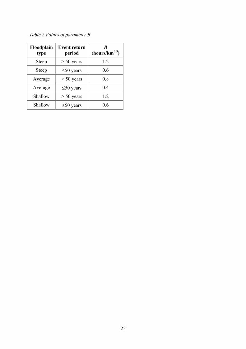
Table 2 Values of parameter B
Floodplain type
Event return period
B (hours/km0.5)
Steep > 50 years 1.2
Steep ≤50 years 0.6
Average > 50 years 0.8
Average ≤50 years 0.4
Shallow > 50 years 1.2
Shallow ≤50 years 0.6
25
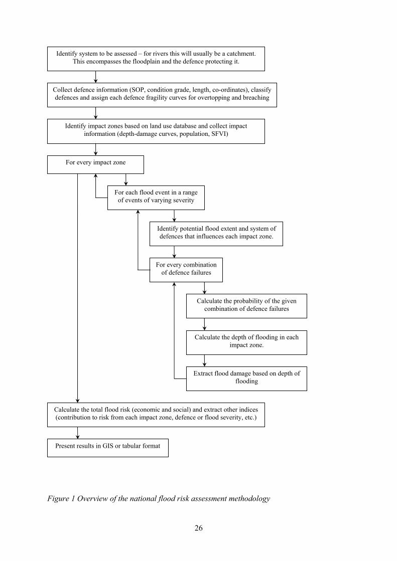
Identify system to be assessed – for rivers this will usually be a catchment. This encompasses the floodplain and the defence protecting it.
Collect defence information (SOP, condition grade, length, co-ordinates), classify defences and assign each defence fragility curves for overtopping and breaching
Identify impact zones based on land use database and collect impact information (depth-damage curves, population, SFVI)
For every impact zone
For each flood event in a range of events of varying severity
Identify potential flood extent and system of defences that influences each impact zone.
Calculate the depth of flooding in each impact zone.
Extract flood damage based on depth of flooding
Calculate the probability of the given combination of defence failures
For every combination of defence failures
Calculate the total flood risk (economic and social) and extract other indices (contribution to risk from each impact zone, defence or flood severity, etc.)
Present results in GIS or tabular format
Figure 1 Overview of the national flood risk assessment methodology
26
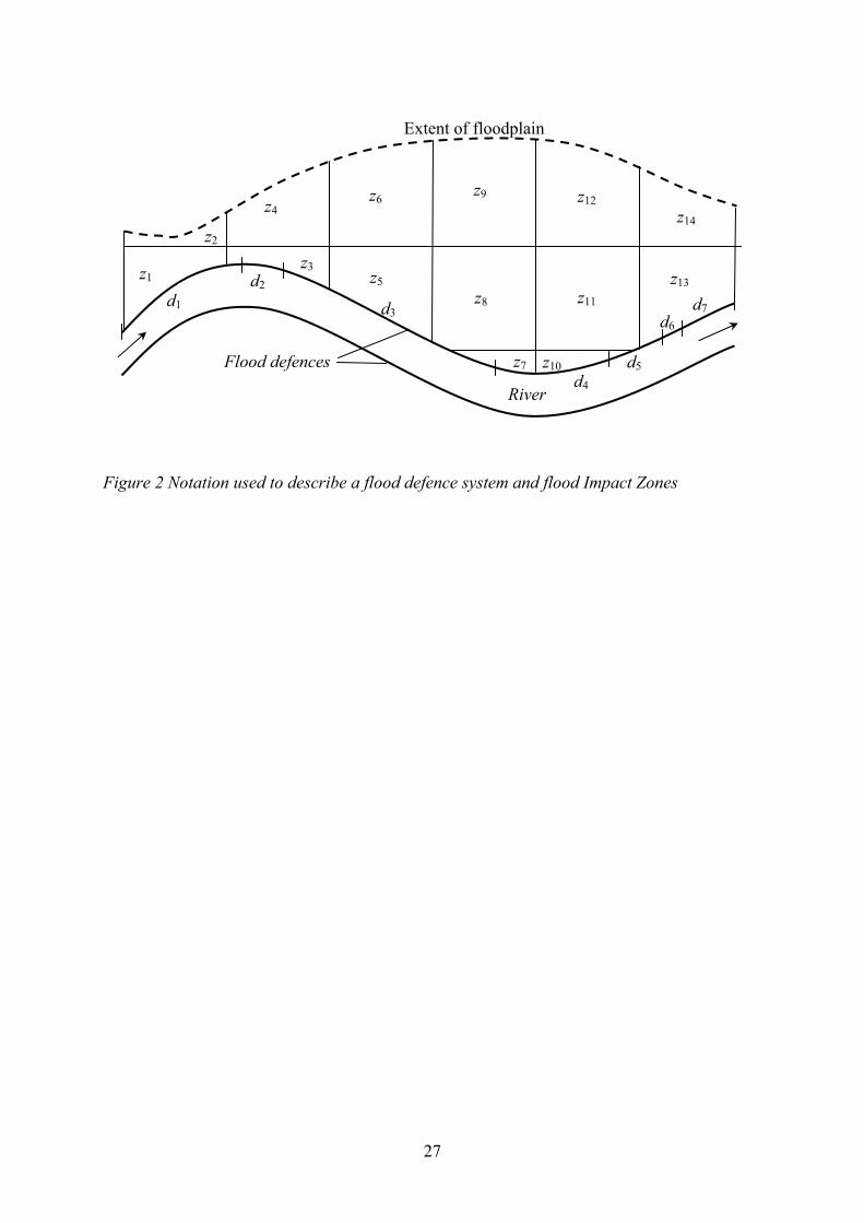
River
z13
z10 z7
z11 z8
Flood defences
z5 z3 z1
d7 d6
d5 d4
d3 d2
d1
z14 z12 z9 z6
Extent of floodplain
z4
z2
Figure 2 Notation used to describe a flood defence system and flood Impact Zones
27
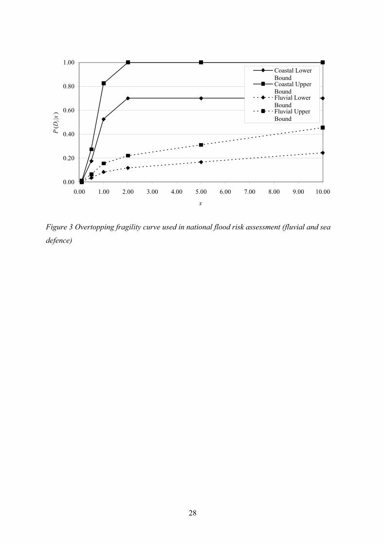
0.00
0.20
0.40
0.60
0.80
1.00
0.00 1.00 2.00 3.00 4.00 5.00 6.00 7.00 8.00 9.00 10.00
x
P(D
i|x)
Coastal LowerBoundCoastal UpperBoundFluvial LowerBoundFluvial UpperBound
Figure 3 Overtopping fragility curve used in national flood risk assessment (fluvial and sea
defence)
28

Flood Defence
Fluvial Coastal
Type 1: Type 2: Type 3: Type 4: Type 5: Type 2: Type 3: Vertical Wall Slope or
Embankment Sloping seawall
or dyke High Ground Culvert Vertical Seawall Beach
Narrow Wide
Front slope protection
Front and crest protection
Front, crest and rear protection
Front slope protection
Front and crest protection
Sheet piles & other materials
Concrete structures
Bricks and masonry
Sheet piles & other materials
Concrete structures
Bricks and masonry
Figure 4 Main classes of flood defences with details of vertical seawall classification
Flood outline
Breach location Defence line
a) U shaped floodplains
Flood outline
Defence line Breach location Downstream
b) V shaped floodplains
IFM boundary Flood outline
Defence line Breach location Downstream
b) V shaped floodplains where flood outline meets boundary of IFM
Figure 5 Assumed flood outlines and depths
31
0
0.2
0.4
0.6
0.8
1
1.2
1.4
1.6
1.8
2
0 10 20 30 40 50 60 70 80 90 100
Percentage of distance from flood defence to floodplain boundary
Med
ian
flood
dep
th
Series1Series2Series3Series4Series5Poly. (Series1)Poly. (Series2)Poly. (Series3)Poly. (Series5)Poly. (Series4)
75-100 yr 50-74 yr 25-49 yr 10-24 yr 1-9 yr
Figure 6 Smoothed median results of statistical data on flood depths across the floodplain for
floods of varying return period (years)22

Expected Annual Damage
High (> £5,000 per Hectare)
Medium ( £1,000 to £5,000 per Hectare)
Low (< £1,000 per Hectare)
0 2 4 6 8 101
Kilometres
Annual likelihood of inundation
High (inundated by 1 in 75 year event)
Medium (inundated by 1 in 200 year event)
Low (not inundated by 1 in 200 year event)
Annual probability of breach/overtopping
0.00 - 0.01
0.01 - 0.05
0.05 - 0.10
0.10 - 0.50
0 1 2 3 40.5Kilometres