A Mathematical Technique for Analyzing Folds With ... - Journals

------ Iraqi Jour. Earth Sci., Vol. 6 , No. 2 , pp. 53-74, 2006 ------

53

A Mathematical Technique for Analyzing Folds With the Computer Program “FOLDPI”

Nabeel K. Al-Azzawi

Department of Geology College of Science Mosul University

(Received 30/4/2006 , Accepted 20/9/2006)

ABSTRACT

A mathematical technique for analyzing folds was proposed instead of the tedious and slow graphical method. Procedure of this technique comprises converting the data of bedding planes to pole attitudes, calculation of the mean pole vector of fold limbs, obtaining the best fit π-circle, determining the fold geometric properties and finding fold cylindricity. This procedure was carried out by FOLDPI, a GWBASIC computer program written for the purpose of this application. Most of the geometrical properties of fold were dealt with. In addition, an example taken from the Sinjar Anticline was used for testing the validity of this technique. The results of testing the program against manually obtained solutions proved that this technique can be very helpful in getting faster and more accurate results ــــــــــــــــــــــــــــــــــــــــــــــــــ

FOLDPIطـريقة رياضية لتحليل الطيات باستخدام البرنامج الحاسوبي

الملخص

). طريقة شكل باي(ُأقترحت هذه الطريقة الرياضية لتحليل الطيات بدالً من الطريقة البيانية السابقة تويات الطبقات إلى وضعيات األقطاب ثم إيجاد االتجـاه تتضمن هذه الطريقة تحويل قراءات وضعيات مس

إن (، حساب معدل وضعية جنـاحي الطيـة والمنطقـة المفصـلية )األقطاب(الجيبتمامي لهذه المتجهات ، أيجاد أفضل دائرة باي تَمر بمعدل وضعية جناحي الطية، حساب الصـفات الهندسـية للطيـة )وجدت

وهو برنامج ُأعد FOLDPIوُألحق بهذه الطريقة البرنامج الحاسوبي . ةوأخيراً إيجاد درجة اسطوانية الطيوقد حللَت طية سنجار بواسطة هذه الطريقة كنموذج الختبـار مـدى . بلغة بيسك لتسريع إنجاز عملياتها

.وكنتيجة، ُأثبت أن هذه الطريقة ليست مشجعة فقط بل إنها أسهل وأسرع وأدق. صالحيتها ــــــــــــــــــــــــــــــــــــــــــــــــــــ

INTRODUCTION Conventionally, folds were analyzed using the common graphical technique of π-

diagram, which is one of the stereographic projection applications. This graphical method has a worldwide usage and it has an advantage of graphically showing fold geometry but it is tedious and time consuming specially in plotting and counting the S-poles on the

Nabeel K. Al-Azzawi

stereonet. Recently, and for the sake of faster and easier techniques, many structural geologists have attempted to modify their related methods towards the trend of mathematics and computer programming approaches. Accordingly, the present author suggests a mathematical technique for digital execution of this π-diagram and the determinion of the geometric parameters of folds using mathematics and computer program.

Previously, some authors made contributions in this trend. They performed some steps in this respect. Ramsay (1967) suggested two mathematical techniques in the scope of fold analysis. The first was applied for determination of unimodal poles distribution by vectors of directional cosines. While the second method was used for determining the best-fit π-circles of cylindrical folds. Bengston (1980) mentioned, marginally, about this idea through out his study of tangent diagram. Ramsay and Huber (1987) described the methods of Ramsay (1967) by “ the accuracy contained in such methods is only justified if it is imperative to exploit the full potential of very precise primary data”.

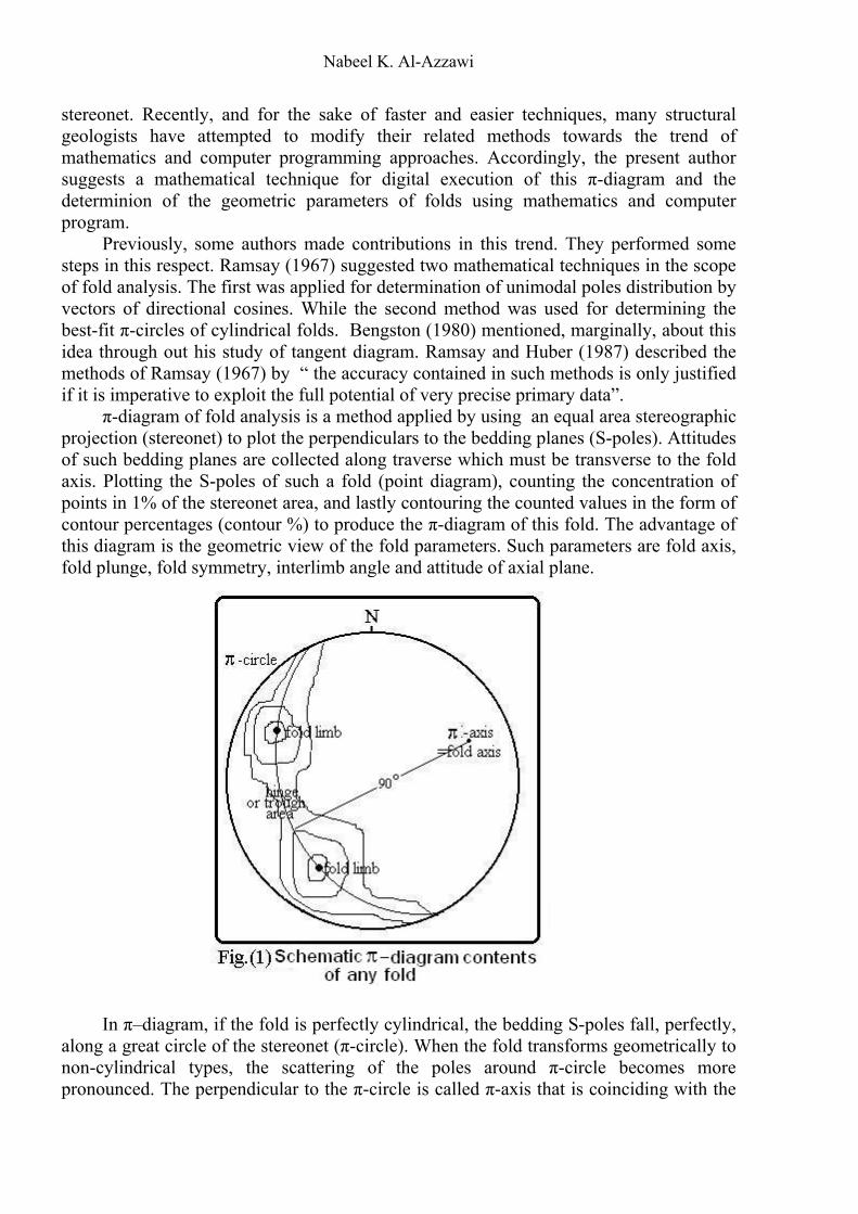
π-diagram of fold analysis is a method applied by using an equal area stereographic projection (stereonet) to plot the perpendiculars to the bedding planes (S-poles). Attitudes of such bedding planes are collected along traverse which must be transverse to the fold axis. Plotting the S-poles of such a fold (point diagram), counting the concentration of points in 1% of the stereonet area, and lastly contouring the counted values in the form of contour percentages (contour %) to produce the π-diagram of this fold. The advantage of this diagram is the geometric view of the fold parameters. Such parameters are fold axis, fold plunge, fold symmetry, interlimb angle and attitude of axial plane.

In π–diagram, if the fold is perfectly cylindrical, the bedding S-poles fall, perfectly, along a great circle of the stereonet (π-circle). When the fold transforms geometrically to non-cylindrical types, the scattering of the poles around π-circle becomes more pronounced. The perpendicular to the π-circle is called π-axis that is coinciding with the

A Mathematical Technique for Analyzing Folds…

fold axis. Consequently, if the fold is perfectly cylindrical the angle between each S-pole and fold axis is perfectly 90° (Fig. 1). Practically, the S-poles of any natural fold do not lie exactly on a certain great circle but fall in zone around this circle. Nevertheless, the human error in field measurements plays a role in the accuracy of these measurements; which amount to ±2 degree (Ramsay and Huber, 1987). However, the mean reason responsible for the scattering of S-poles is the absence of perfectly cylindrical folds in the field. Many of natural folds are of cylindrical, sub-cylindrical and non-cylindrical styles. In this respect Ramsay (1967) designed his method for determining the best-fit π-circles for perfectly cylindrical folds. This is because only in this type of folds the π-axis makes a right angle with each S-pole; and he built up his mathematics on this property. It must be mentioned that in Ramsay (1967) terminology, the term cylindrical fold is analogous to perfectly cylindrical one. In the more recent synthesis, Ramsay and Huber (1987) classified the folds into perfectly cylindrical, cylindrical, sub-cylindrical and non-cylindrical types (Fig. 2). Previously, folds classified as cylindrical and non-cylindrical and some time cylindroid (Fleuty, 1964). In the classification of Ramsay and Huber(1987) the perfectly cylindrical fold has its S-poles lie perfectly on the π-circle.

While if more than 90% of the S-poles fall within an angle of ±10° from the

constructed π–circle the fold should be termed cylindrical. But if more than 90% of the data lie within ±20° of the π -circle the fold is then called sub-cylindrical fold. Folds with more than 10% of their S-poles falling outside the limit of ±20° are termed non-cylindrical (Fig. 2). In addition to the scope of the present work, the author extended the method of Ramsay (1967) from its application only on perfectly cylindrical to include all types of folds described by Ramsay and Huber (1987). This extension was based on the styles of poles distribution a round the best-fit π-circle.

Nabeel K. Al-Azzawi

METHODOLOGY The proposed mathematical method comprises the following procedures:

1st- Converting the data of bedding plane attitudes of both fold limbs (strike direction/dip amount when strike was taken clockwise from dip direction) to pole attitude (dip direction/dip amount) and finally to their corresponding directional cosine vectors (α, β & γ).

2nd- Calculation of the mean vector of each fold limb and hinge area by unimodal poles distribution method (summing method).

3rd- Obtaining the best-fit π-circle for these two means of fold limbs, or three means (two limbs and a hinge area)

4th- Determination of fold parameters which reflect its geometry. 5th- Determination of the cylindricity of folds according to Ramsay and Huber (1987). 1st- Determination of directional cosines :

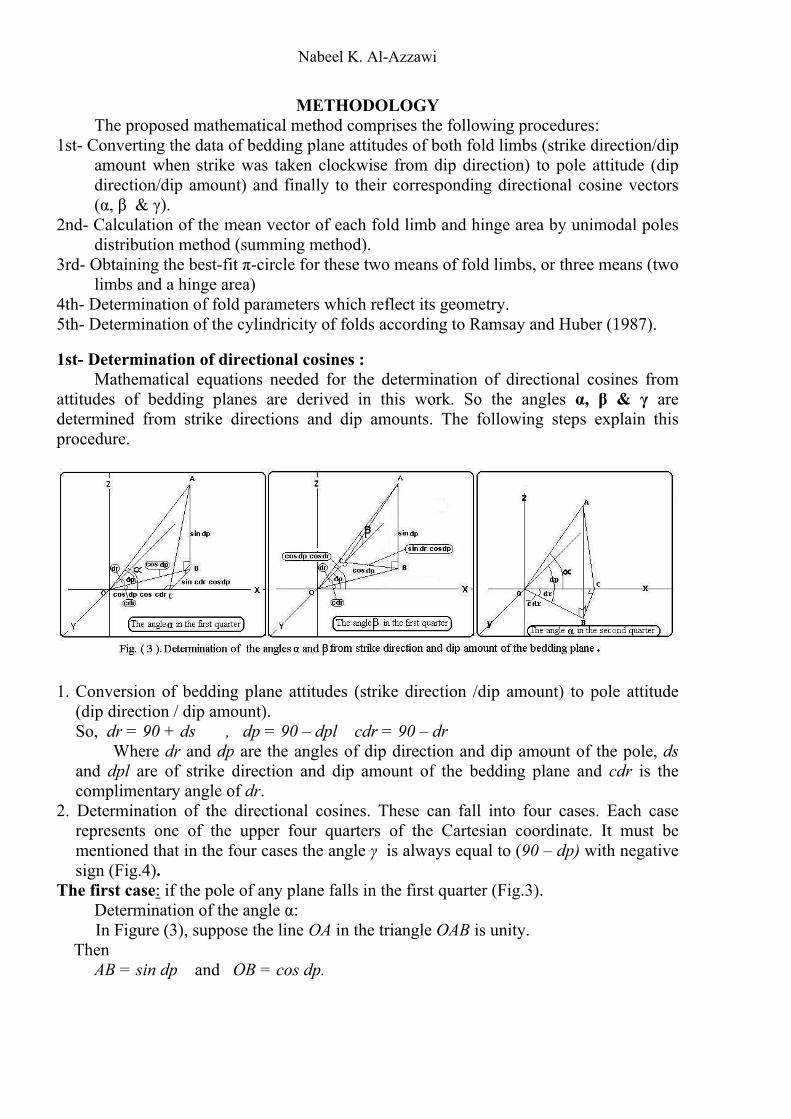
Mathematical equations needed for the determination of directional cosines from attitudes of bedding planes are derived in this work. So the angles α, β & γ are determined from strike directions and dip amounts. The following steps explain this procedure.

1. Conversion of bedding plane attitudes (strike direction /dip amount) to pole attitude

(dip direction / dip amount). So, dr = 90 + ds , dp = 90 – dpl cdr = 90 – dr

Where dr and dp are the angles of dip direction and dip amount of the pole, ds and dpl are of strike direction and dip amount of the bedding plane and cdr is the complimentary angle of dr.

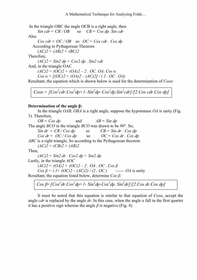
2. Determination of the directional cosines. These can fall into four cases. Each case represents one of the upper four quarters of the Cartesian coordinate. It must be mentioned that in the four cases the angle γ is always equal to (90 – dp) with negative sign (Fig.4).

The first case: if the pole of any plane falls in the first quarter (Fig.3). Determination of the angle α:

In Figure (3), suppose the line OA in the triangle OAB is unity. Then

AB = sin dp and OB = cos dp.


In the triangle OBC the angle OCB is a right angle, then Sin cdr = CB / OB so CB = Cos dp. Sin cdr

Also Cos cdr = OC / OB so OC = Cos cdr . Cos dp

According to Pythagorean Theorem (AC)2 = (AB)2 + (BC)2

Therefore, (AC)2 = Sin2 dp + Cos2 dp . Sin2 cdr

And, in the triangle OAC (AC)2 = (OC)2 + (OA)2 – 2 . OC. OA. Cos α Cos α = [(OC)2 + (OA)2 – (AC)2] / ( 2 . OC . OA)

Resultant, the equation which is shown below is used for the determination of Cosα: Determination of the angle β:

In the triangle OAB, OBA is a right angle, suppose the hypotenuse OA is unity (Fig. 3). Therefore,

OB = Cos dp and AB = Sin dp The angle BCO in the triangle BCO was drawn to be 90°. So,

Sin dr = CB / Cos dp so CB = Sin dr . Cos dp Cos dr = OC / Cos dp so OC = Cos dr . Cos dp

ABC is a right triangle, So according to the Pythagorean theorem (AC)2 = (CB)2 + (AB)2

Then, (AC)2 = Sin2 dr . Cos2 dp + Sin2 dp

Lastly, in the triangle AOC (AC)2 = (OA)2 + (OC)2 – 2 . OA . OC . Cos β Cos β = ( 1+ (OC)2 – (AC)2) / (2 . OC ) ------ OA is unity

Resultant, the equation listed below, determine Cos β:

It must be noted that this equation is similar to that equation of Cosα, accept the angle cdr is replaced by the angle dr. In this case, when the angle α fall in the first quarter it has a positive sign whereas the angle β is negative (Fig. 4).

Cos β=[Cos2dr.Cos2dp+1- Sin2dp-Cos2dp. Sin2dr]/[2.Cos dr.Cos dp]

Cosα = [Cos2cdr.Cos2dp+1–Sin2dp–Cos2dp.Sin2cdr]/[2.Cos cdr.Cos dp]

Nabeel K. Al-Azzawi

The second case: If the pole of any plane falls in the second quarter (Fig. 3). Therefore, drnew = drold – 90 cdr = 90 – dr

Similar to the first case, the angle α and β can be determined by: And,

In this case, both α and β have positive signs (Fig. 4).

The third case: If the pole of any plane falls into the third quarter. Then, drnew = drold – 180 cdr = 90 - dr Similarly, And In this quarter, α has negative sign. While β is positive (Fig. 4). The forth case: When the pole lies in the forth quarter. Therefore, drnew = dr old –270 cdr = 90 – dr

Similar to the previous cases, the angles α and β can be determined by the following equations: And

Cosα = [Cos2dr.Cos2dp+1–Sin2dp–Cos2dp.Sin2dr]/[2.Cos dr.Cos dp]

Cos β=[Cos2cdr.Cos2dp+1- Sin2dp-Cos2dp. Sin2cdr]/[2.Cos cdr.Cos dp]

Cosα = [Cos2cdr.Cos2dp+1–Sin2dp–Cos2dp.Sin2cdr]/[2.Cos cdr.Cos dp]

Cos β=[Cos2dr.Cos2dp+1- Sin2dp-Cos2dp. Sin2dr]/[2.Cos dr.Cos dp]

Cosα = [Cos2dr.Cos2dp+1–Sin2dp–Cos2dp.Sin2dr]/[2.Cos dr.Cos dp]


In this quarter, the angles α and β have negative signs. Resultant, data of poles (directions and dip amounts) representing bedding planes are converted to directional cosines which represented by the cosines of the angles α, β and γ. 2nd- The unimodal pole distribution method:

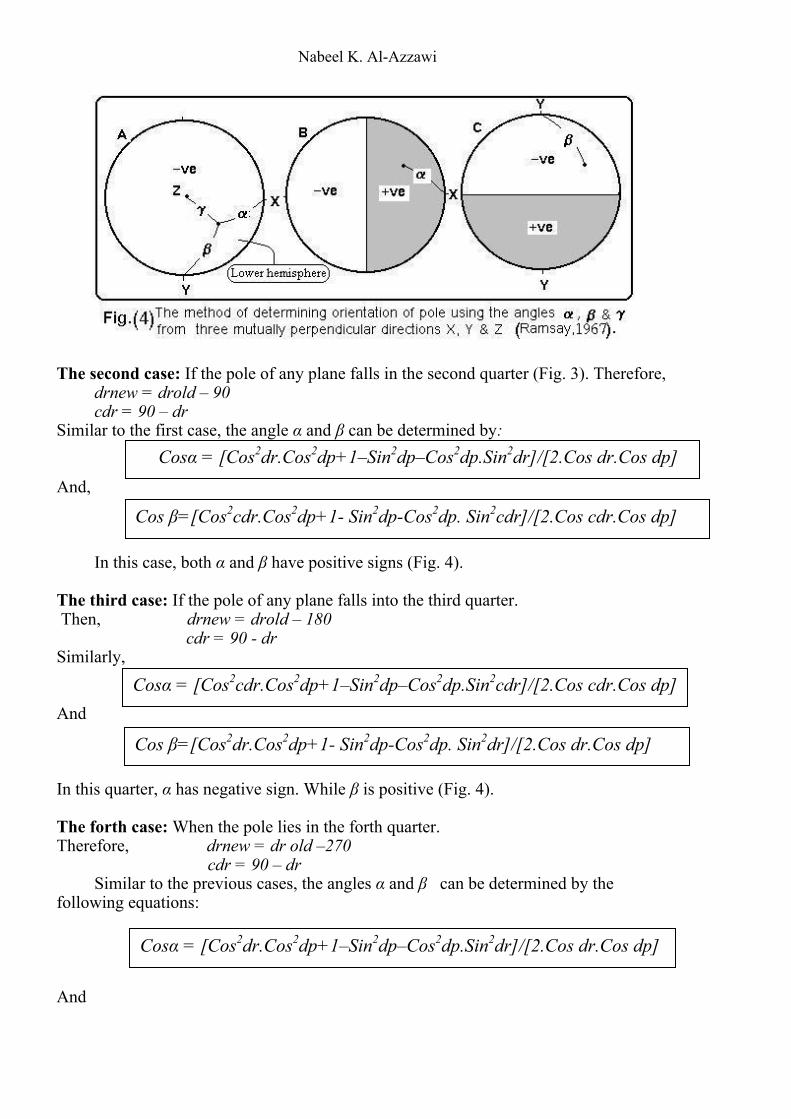
The unimodal pole distribution was suggested and described by Ramsay (1967). It is also called method of summing vectors. Considering the pole as a unit vector, the method is used for determining the mean vector of poles of any geologic planes. This is done after determining the angles α, β and γ of each pole (unit vector) with respect to the coordinate axes x, y and z respectively (Fig. 5A). These angles, in the present work, are an output of the previous procedure (mentioned in 1st). The x, y, and z components of the side of the vector box (Fig. 5B) for each measurement are then calculated by Cosα, Cosβ and Cosγ respectively. These directional cosines are determined for all poles and sums of the vector components are calculated (Σ cosα, Σ cosβ and Σ cosγ). These sums give the dimentions of the x, y, and z components of the total vector sum and the diagonal of this box gives the strength of the total vector sum (TVS) which is equal to:

TVS = [(Σcosα )2 + (Σcosβ )2 + (Σcosγ )2]1/2 ------ (Ramsay,1967) Therefore, the mean vector direction with respect to x, y and z axes are given by: Cosα⎯ = Σcosα / TVS ----------------------- 1 Cosβ⎯ = Σcosβ / TVS ----------------------- 2 Cosγ⎯ = Σcosγ / TVS ------------------------ 3

In the course of this work, data that were taken from a fold can be differentiated into

two or three concentrations. If the folds are of chevronic or mostly chevronic style, two concentrations of pole distribution are found. That is because the hinge is angular and there is no hinge area then the two concentrations representing the two limbs. Whereas, in the box type folds or near this shape, three concentrations are found. Two of them for the limbs and the third represent the hinge area. It means that each fold has two or three mean vectors. Consequently, the users of this method (Unimodal poles distribution) must process each concentration of fold poles and determine the mean vector of each one. These mean vectors (with the angles α, β and γ) can be used for determining the best-fit

Cos β=[Cos2cdr.Cos2dp+1- Sin2dp-Cos2dp. Sin2cdr]/[2.Cos cdr.Cos dp]

Nabeel K. Al-Azzawi

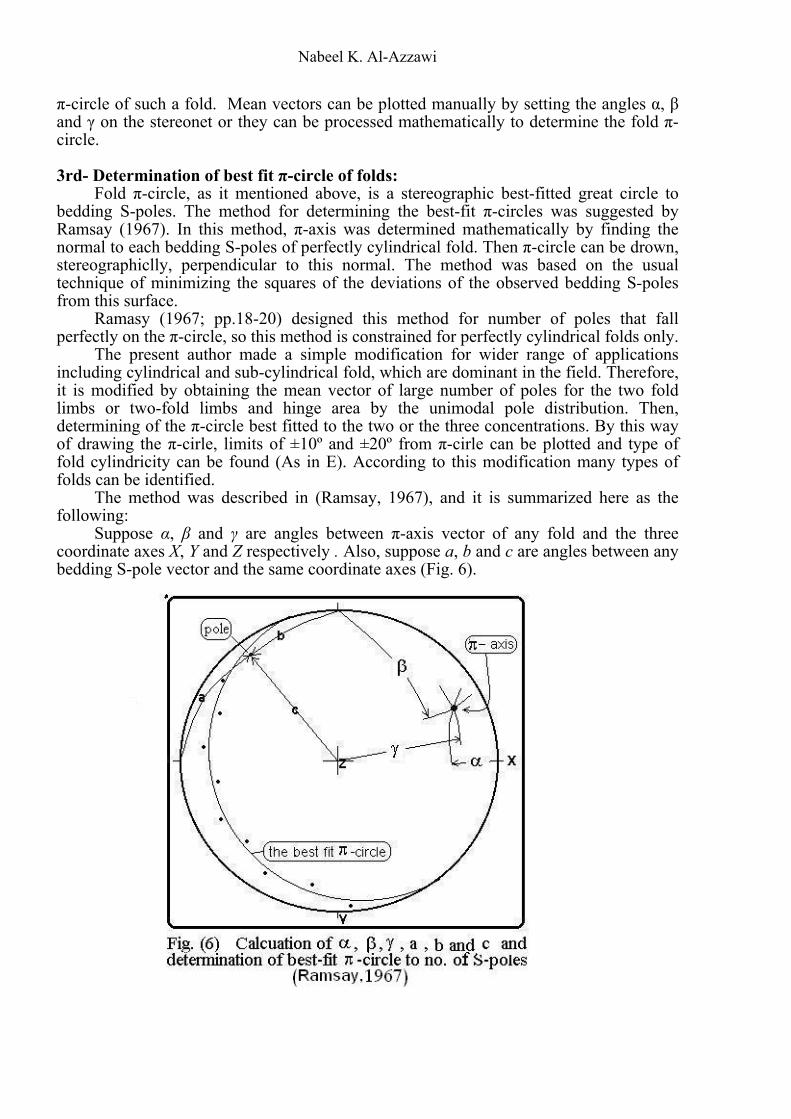
π-circle of such a fold. Mean vectors can be plotted manually by setting the angles α, β and γ on the stereonet or they can be processed mathematically to determine the fold π-circle. 3rd- Determination of best fit π-circle of folds:

Fold π-circle, as it mentioned above, is a stereographic best-fitted great circle to bedding S-poles. The method for determining the best-fit π-circles was suggested by Ramsay (1967). In this method, π-axis was determined mathematically by finding the normal to each bedding S-poles of perfectly cylindrical fold. Then π-circle can be drown, stereographiclly, perpendicular to this normal. The method was based on the usual technique of minimizing the squares of the deviations of the observed bedding S-poles from this surface.

Ramasy (1967; pp.18-20) designed this method for number of poles that fall perfectly on the π-circle, so this method is constrained for perfectly cylindrical folds only.

The present author made a simple modification for wider range of applications including cylindrical and sub-cylindrical fold, which are dominant in the field. Therefore, it is modified by obtaining the mean vector of large number of poles for the two fold limbs or two-fold limbs and hinge area by the unimodal pole distribution. Then, determining of the π-circle best fitted to the two or the three concentrations. By this way of drawing the π-cirle, limits of ±10º and ±20º from π-cirle can be plotted and type of fold cylindricity can be found (As in E). According to this modification many types of folds can be identified.

The method was described in (Ramsay, 1967), and it is summarized here as the following:

Suppose α, β and γ are angles between π-axis vector of any fold and the three coordinate axes X, Y and Z respectively . Also, suppose a, b and c are angles between any bedding S-pole vector and the same coordinate axes (Fig. 6).


A = ( Σ lm Σmn – Σl n Σ m2 ) / ( Σ l2 Σm2 – (Σ lm)2 ) B = ( Σ lm Σ ln – Σ mn Σ l2 ) / ( Σ l2 Σ m2 – (Σ lm)2 )

Where, cos a = l , cos b = m, cos c = n, cos α / cos γ = A and cos β / cos γ = B Ramsay (1967) derived three equations for determination of α, β and γ. These

equations are described below. Because, cos2 α + cos2 β + cos2 γ = 1 And A = cos α / cos γ and B = cos β / cos γ Therefore A2 Cos2 γ + B2 cos2 γ + cos2 γ = 1 cos2 γ (A2 + B2 + 1) = 1 And cos2 γ = 1/ (A2 + B2 + 1) so Similarly, equations responsible for determining α and β were derived.

By the values and signs of these angles the Cartesian coordinate position of π-axis was found. Fold π- circle can be drawn considering this π-axis normal to it. 4th- Determination of fold geometry:

Most of the important geometric properties of folds can be determined from this technique. Such properties are fold axis, fold plunge, interlimb angle, fold symmetry, attitude of axial plane and fold cylindricity. Fold axis:

The angles α, β and γ which were calculated in (3rd page 6 ) are used for determining the attitude of fold axis (dip direction / dip amount). From figure (7),

Also from the same figure, the triangle OAC has the right angle OCA and the hypotenuse OA suppose to be unity.

dp = 90 – γ when dp is the dip amount of fold axis

cos γ = ( 1+ A2 + B2 ) –1/2

cos α = A (1 + A2 + B2 ) -1/2

cos β = B ( 1+ A2 + B2 ) –1/2

Nabeel K. Al-Azzawi

AC = sin β and OC = cos β Also in the triangle, OBA is a right angle.

OB = cos dp and AB = sin dp Whereas in the triangle ABC

AC2 = AB2 + CB2 CB = (sin2 β – sin2 dp)1/2

In the triangle OBC, CB2 = OC2 + OB2 – 2. OC. OB.Cos dr Sin2 β – sin2 dp = cos2 β . cos2 dp – 2 .cos β .cos dp . cos dr 2. cos β . cos dp . cos dr = cos2 β + cos2dp –sin2 β + sin2 dp

When dr is the dip direction of fold axis. The signs of the angles α and β serve as

indicators to show in which quarter of Cartesian coordinate the fold axis was fall (Table 1).

Table 1 : Signs of the angles α and β in each coordinate quarter.

Sign of the angle α Sign of the angle β Position Positive Negative First quarter Positive Positive Second quarter Negative Positive Third quarter Negative Negative Forth quarter

If the fold axis falls in the first quarter, dr remains without change. Whereas, if it

falls in the second, third and forth quarter, then 90°, 180° and 270° are added to the angle dr for obtaining its correct dip direction). Fold plunge:

Fold plunge depends upon dip amount of fold axis (dp). When (dp) is equal to zero, the fold is nonplunging. While if (dp) is more than zero, the fold becomes plunging. And increasing of dp angle means increasing of degree of plunging. Interlimb angle:

According to this procedure, interlimb angle can be calculated by adding the absolute value of γ1 (of the first limb) to the absolute value of γ2 (of the second one). The angles γ1 and γ2 are always having negative sign (Fig.4) then it must be considered their absolute values when the interlimb angle was determined. This calculation must be done along a plane perpendicular to the fold axis. Then concentrations of the two limbs must be rotated until the fold axis becomes horizontal and determination of the interlimb angle was done along the N-S vertical plane (Fig. 8).

dr = cos-1 [ (cos2β+cos2dp- sin2β +sin2dp)/(2*cos β* cosdp)]

Attitude of fold axis = dip direction (dr) / dip amount (dp)

Fold Plunge = dp of fold axis


Where adpl1 and adpl2 are mean dips of the two limbs Folds symmetry:

Fold symmetry can be found by comparing adpl1 with adpl2 or γlimb1 with γlimb2. Resultant, if dpl1 is equal to dpl2. Then the fold is symmetrical, otherwise it is asymmetrical with the vergency being towards the limb which has greater pole dip angle (dp). Attitude of axial plane:

This attitude will be possible if the attitude of axial trace is known (Ramsay and Huber, 1987). While if the fold is of parallel type, axial plane can be obtained by joining the bisector of interlimb angle with the fold axis. This is because in the parallel fold the axial plane always bisects the interlimb angle. In this work the axial plane determination was restricted to parallel fold type because other types are more complicated to be processed mathematically.

Axial plane attitude can be represented by its dip amount Apdp and dip direction Apdr.

Apdp= 90 – ((( γmax + γmin ) / 2) – γmin ) Where γmax and γmin are dip angles of steep and gentle limbs respectively.

Apdr coincide with the dip direction of gentle limb.

5th- Determination of fold cylindericity: Ramsay and Huber (1987) classified the folds into perfectly cylindrical, cylindrical,

sub-cylindrical and non-cylindrical, which were described previously in the introduction (Fig. 2).

Interlimb angle = γlimb1 + γlimb2 = 180- (adpl1 + adpl2 )

Folds symmetry : adpl1 < = > adpl2 OR γlimb1 <=> γlimb2

Attitude of axial plane = Apdp / Apdr

Nabeel K. Al-Azzawi

Different natural folds show different properties or different π-diagram models. And it is very complicated to put a solution for each model. So a simplification was made for putting a general procedure for all these models. This is to revolve and rotate the data (mentioned below) to make a general solution for all the cases and keeping the entire relative geometrical relationships constant with each other but not with the coordinate axes. Revolving and rotating fold data

Many authors suggested various methods for rotation of oriented data. Saha (1987) designed a FORTRAN program for rotation of data by transformation matrix. Al-Azzawi and Al-Jumaily (2000) proposed a mathematical procedure for rotation of joint planes relative to bedding rotation by trigonometric method.

For the sake of applying this idea, two stages are used. Firstly, revolving of data, horizonally, until direction of π-axis coincides with east direction of stereonet. This is done by adding (90 – dr) when dr less than 90°, and subtracting (dr – 90) when dr more than 90° to or from the angle dr.

Secondly, rotation of all data around Y coordinate axis ( N-S line in the stereonet) until π-axis becomes horizontal; it means rotation angle (R) = dp of π-axis (Fig. 8). When π-axis rotated by the angle R , π-circle became vertical plane. This is because π-axis is always perpendiocular to the plane containing bedding S-poles (π-circle). This rotation can be done by transformation matrix. Many authors such as Arfken (1970) and Saha (1987) described this method. And it is summarizes here by the followings: 1- Determination of L, M & N components for each S-pole vector before rotation.

L = cos dp . sin dr , M = cos dp . cos dr and N = sin dp 2- Multiplication of the components L, M & N by the transformational matrix that is

responsible for rotation of vectors anticlockwise around Y-axis and through an angle R.

L cos R 0 sin R M * 0 1 0

N -sin R 0 cos R

The resultant are new L, M & N components ( after rotation)which are used to determine the direction dr and dip angle dp of a pole vector.

Mathematically, this fold classification could not be applied without revolving and rotating data (as it mentioned above). Rotating all data until π-axis becomes horizontal standardize all natural cases in into one form. Figure (9) shows the rotated state of Figure (2) which responsible for this classification. Figure (9) can be used to plot the revolved and rotated bedding S-poles of any fold and to find the type of this fold according to its cylindricity.

If dr < 90 then dr = dr + (90 – dr ) clockwise rotation Wheras, if dr > 90 then dr = dr – (dr – 90) anticlockwise

dp = sin-1 Nnew and dr = sin-1 (Lnew / cos dp) or dr = cos-1 (Mnew / cos dp)


Ramsay and Huber (1987) suggested limits for difining fold cylindricity (Fig. 2). These limits are ±10 and ±20 around π-circle of perfect cylindrical fold. These limits were divided the stereonet into fields; each field represents one of fold types. Figure (9) showed these limits after revolution and rotation. Empirically, the present author derived mathematical equations to deal with these limits during the present technique. And using Lagrangian interpolation method mentioned in (Al-Azzawi, 2004) does this. For more explanation, the author exhibited curves shown in figure (10) representing these limits

S-pole directions of stereonet normally range from 1° to 360°. So that, direction of

each S-pole can be tested and determined in which field it fall. Counting of these poles and obtaining the percentage of each field was done. Then the fold can be classifying as in the followings: 1- If all S-poles fall on the plane of perfectly cylindrical (π-circle) (Fig. 11), then it is

called perfectly cylindrical fold. 2- If 90% of S-poles fall between plane-10 and plane+10 around the mean π-circle

(Fig.9) or on and above the standard curve of cylindrical fold (Fig. 10), then the fold named cylindrical type.

Nabeel K. Al-Azzawi

3- If 90% of them fall between plane-20 and plane+20 (Fig.9) or on and above the standard curve of sub-cylindrical fold (Fig.10), the fold classified as sub-cylindrical type.

4- Otherwise or when more than 10% of the S-poles lie outside plane-20 and plane+20 (Fig.9) or fall below the standard curve of sub-cylindrical fold (Fig.10), the fold becomes non-cylindrical type.

So, mathematically or by computer programming, the number of bedding S-poles that fall between these limits can be determined.

The procedure for analyzing fold was designed in GWBASIC computer program called FOLDPI (see the Appendix) Tested sample:

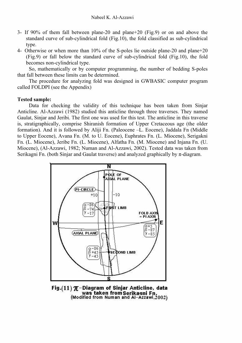
Data for checking the validity of this technique has been taken from Sinjar Anticline. Al-Azzawi (1982) studied this anticline through three traverses. They named Gaulat, Sinjar and Jeribi. The first one was used for this test. The anticline in this traverse is, stratigraphically, comprise Shiranish formation of Upper Cretaceous age (the older formation). And it is followed by Aliji Fn. (Paleocene –L. Eocene), Jaddala Fn (Middle to Upper Eocene), Avana Fn. (M. to U. Eocene), Euphrates Fn. (L. Miocene), Serigakni Fn. (L. Miocene), Jeribe Fn. (L. Miocene), Alfatha Fn. (M. Miocene) and Injana Fn. (U. Miocene), (Al-Azzawi, 1982; Numan and Al-Azzawi, 2002). Tested data was taken from Serikagni Fn. (both Sinjar and Gaulat traverse) and analyzed graphically by π-diagram.


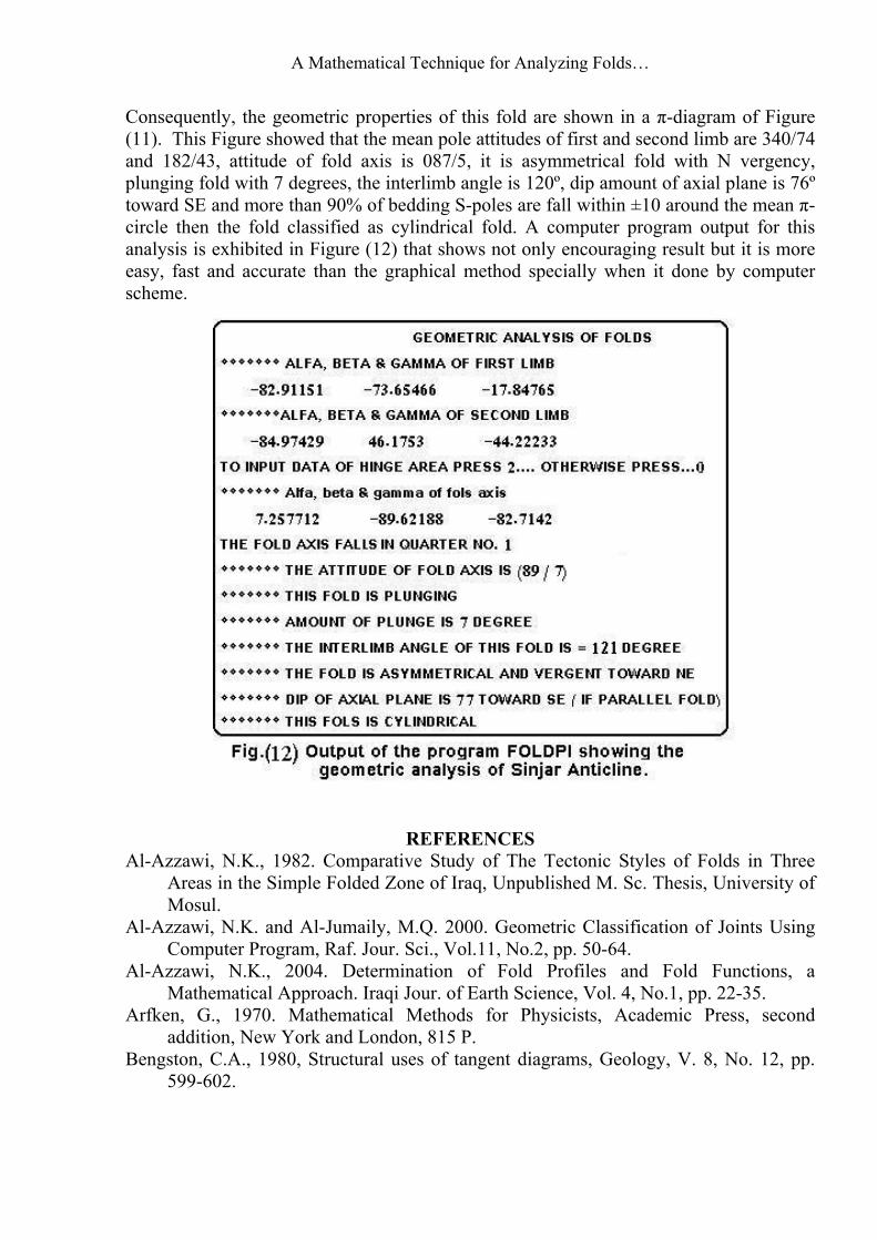
Consequently, the geometric properties of this fold are shown in a π-diagram of Figure (11). This Figure showed that the mean pole attitudes of first and second limb are 340/74 and 182/43, attitude of fold axis is 087/5, it is asymmetrical fold with N vergency, plunging fold with 7 degrees, the interlimb angle is 120º, dip amount of axial plane is 76º toward SE and more than 90% of bedding S-poles are fall within ±10 around the mean π-circle then the fold classified as cylindrical fold. A computer program output for this analysis is exhibited in Figure (12) that shows not only encouraging result but it is more easy, fast and accurate than the graphical method specially when it done by computer scheme.

REFERENCES Al-Azzawi, N.K., 1982. Comparative Study of The Tectonic Styles of Folds in Three

Areas in the Simple Folded Zone of Iraq, Unpublished M. Sc. Thesis, University of Mosul.

Al-Azzawi, N.K. and Al-Jumaily, M.Q. 2000. Geometric Classification of Joints Using Computer Program, Raf. Jour. Sci., Vol.11, No.2, pp. 50-64.

Al-Azzawi, N.K., 2004. Determination of Fold Profiles and Fold Functions, a Mathematical Approach. Iraqi Jour. of Earth Science, Vol. 4, No.1, pp. 22-35.

Arfken, G., 1970. Mathematical Methods for Physicists, Academic Press, second addition, New York and London, 815 P.

Bengston, C.A., 1980, Structural uses of tangent diagrams, Geology, V. 8, No. 12, pp. 599-602.

Nabeel K. Al-Azzawi

Fleuty, M.J., 1964. The Description of Folds, Proc. Geol. Assoc.London, Vol.75, pp.461-492.

Numan, N.M.S. and Al-Azzawi, N.K., 2002. Progressive Versus Paroxysmal Alpine Folding in Sinjar Anticline Northwest Iraq, Iraqi Jour. Of Earth Science, Vol. 2, No. 2, pp.59-69.

Ramsay, J.G. and Huber, M.I., 1987. The techniques of modern structural geology: V.2, folds and Fractures, Academic Press, London, UK, 700p.

Ramsay, J.G., 1967. Folding and fracturing of rocks, McGraw Hill, New York, 568. Saha, D., 1987. SPIN8: A FORTRAN 77 Program for Automated Rotation of Poles,

Computers and Geosciences, Vol.13, No. 3, pp. 235-254.


APPENDIX 10 REM FOLDPI 20 REM PROGGRAM FOR ANALIZING FOLDS BY NEW MATHEMATICAL TECHNIQUE 30 REM DEPENDING ON THE PI- DIAGRAM PRINCIPALS . WRITTEN BY DR. NABEEL K . 40 REM AL –AZZAWI, JONE ,2005. DEPARTEMENT OF GEOIOGY/UNIVERSITY OF MOSUL. 50 CLS. 60 PRINT 70 PRINT “ GEOMETRIC ANALYSIS OF FOLDS “ 80 PRIN “ 90 PRINT 100 N1=50 110 N2=15 120 N3=0 130 K=N1+N2 140 M=N1+N2 +N3 150 DIM DS(M), DPL(M), DR(M), DR1(M), DR2(M), DR3(M), DRR(M), DP(M), DP1(M), DP2(M), DPP(M), CDR(M), ALFA(M), BETA(M), GAMA(M), OFIE1(M), OFIE2(M), COSALF(M), COSBET(M),COSGAM(M), X(10), FX(10), LU(10), LD(10) 160 CINDY=1 170 REM INPUT DATA OF BEDDING PLANES AS STRIKE DIRECTIONS / DIP AMOUNTS. 180 IF CINDY=1 THEN PRINT”*********ALFA, BETA & GAMMA OF FIRST LIMB” 190 IF CINDY=2 THEN PRINT”*********ALFA, BETA & GAMMA OF SECOND LIMB” 200 IF CINDY=3 THEN PRINT”*********ALFA, BETA & GAMMA OF HINGE AREA” 210 ON CINDY GOTO 220,230,240 220 N = N1 : GOTO 250 230 N = N2 : GOTO 250 240 N = N3 250 SDPL=0 260 SDDR=0 270 FOR I = 1 TO N 280 READ DS(I) , DPL(I) 290 SDPL = SDPL +DPL(I) 300 DDR = DS(I) – 90 310 SDDR = SDDR + DDR 320 NEXT I

330 DATA 234,16, 240,17, 246,15, 242,18, 240,18, 242, 17, 260,21,242,18, 252,20, 240,23,248, 23,15, 250,13, 236, 13, 250,10, 270,18, 248,20 340 DATA 236,19, 240, 18, 242,12, 256, 12, 250,10, 244,12, 250,14, 236, 16, 240, 20, 260,18 ,268,20, 250,

18,264, 21, 252, 18,264, 20, 240,20 350 DATA 230, 20,240,20, 260, 20, 286,22,242, 20, 232, 22, 250, 23, 230,32,228, 30,230,18, 252, 20, 254,12,18,

248, 15,258, 20, 258,15 360 DATA 100, 25, 110, 28, 90, 60, 89, 69, 100, 60, 80, 42, 74, 43, 90, 42, 100, 37, 87,45,100,45, 88, 49, 94, 42,

98, 34, 79, 45 370 ADPL(CINDY) = INT(SDPL/N) 380 ADDR(CINDY) = INT(SDDR/N) 390 IF ADDR(CINDY) < 0 THEN ADDR(CINDY) = 360 – ADDR(CINDY) 400 SDR=0 410 FOR I = 1 TO N 420 REM DR AND DP ARE DIP DIRECTION AND DIP AMOUNT OF S-POLE, 430 REM WHERE CDR IS THE COMLIMENTARY ANGLE OF DR. 440 DR(I) = 90+ DS(I) :DP(I) = 90- DPL(I) : IF DR(I) > 360 THEN DR(I) = DR(I) –360 450 SDR = SDR + DR(I) 460 REM THE THREE STATEMENTS BELOW ARE TO PUT ALL READINGS (OF 2 LIMBS AND HINGEA REA) IN ONE ARRY. 470IF CINDY = 1 THEN DR2(I) = DR(I) : DP2(I) = DP(I) 480 IF CINDY=2 THEN DR2( I+ N1 ) =DR ( I ) : DP2 (I+N1) =DP ( I ) 490 IF CINDY=3 THEN DR2 ( I + K ) = DR ( I ) : DP2 (I + K )= DPI 500 IF DR (I )<=90 THEN DR1 ( I )=DR ( I ) 510 IF DR ( I )> 90 AND DR ( I ) <=180 THEN DR1 ( I )=DR ( I ) - 90

Nabeel K. Al-Azzawi

520 IF DR ( I ) > 180 AND DR ( I )<=270 THEN DR1 ( I )= DR ( I ) – 180 530 IF DR ( I ) >270 AND DR ( I ) <=360 THEN DR1 ( I )=DR ( I ) –270 540 CDR ( I )= 90 – DR1 ( I ) 550 DR1 ( I ) = DR1 ( I ) * 3.132857 / 180 560 DP ( I )=DP ( I ) * 3.142857 / 180 : CDR ( I )= CDR ( I ) * 3. 142857 / 180 570 NEXT I 580 ADR(CINDY) = SDR/N 590 REM DETERMINATION OF DIRECTIONAL COSINES: THERE ARE FOUR CASES. 600 REM GAMMA=90-DP WITH -VE SIGN. 610 FOR I = 1 TO N 620 GAMA(I) = 90 – DP(I) * 180 / 3.142857 630 GAMA(I) = GAMA(I) * 3.142857 / 180 640 IF GAMA(I) > 0 THEN GAMA(I) = 0 – GAMA(I)

650 OFIE1 (I) = ((COS(CDR(I)))^2 * (COS(DP(I)))^2 + 1 –(SIN(DP(I)))^2- (COS(DP(I)))^ 2 *SIN(DR1(I))) ^2) / (2 * COS(DR1(I)) * COS(DP(I)))

670 IF DR(I) > 90 THEN 750 680 COSALF(I) = OFIE1(I) 690 COSBET(I) = OFIE2(I) 700 ALFA(I) = ATN(SQR(1- (OFIE1(I)) ^2) / OFIE1(I)) 710 BETA(I) = ATN(SQR(1- ( OFIE2(I))^2) / OFIE2(I)) 720 IF ALFA(I) < 0 THEN ALFA(I) = 0 - ALFA(I) 730 IF BETA(I) > 0 THEN BETA(I) = 0 – BETA(I) 740 GOTO 980 750 IF DR(I) > 180 THEN 830 760 COSALF(I) = OFIE2(I) 770 COSBET(I) = OFIE1(I) 780 ALFA(I) = ATN(SQR(1- ( OFIE2(I))^2) / OFIE2(I)) 790 BETA(I) = ATN(SQR( 1- ( OFIE1(I))^2) / OFIE1(I)) 800 IF ALFA(I) < 0 THEN ALFA(I) = ALFA(I) * (-1) 810 IF BETA(I) < 0 THEN BETA(I) = BETA(I) * (-1) 820 GOTO 980 830 IF DR(I) > 270 THEN 910 840 COSALF(I) = OFIE1(I) 850 COSBET(I) = OFIE2(I) 860 ALFA(I) = ATN ( SQR( 1 – (OFIE1(I))^2) / OFIE1(I)) 870 BETA (I) = ATN) SQR( 1 – ( OFIE2(I)^2) / OFIE2(I)) 880 IF ALFA(I) > 0 THEN ALFA(I) = 0 – ALFA(I) 890 IF BETA(I) < 0 THEN BETA(I) = 0- BETA(I) 900 GOTO 980 910 REM WHEN DR MORE THAN 270 . 920 COSALF(I) = OFIE2(I) 930 COSBET(I) = OFIE1(I) 940 ALFA(I) = ATN(SQR( 1 – (OFIE2(I))^2) / OFIE2(I)) 950 BETA(I) = ATN(SQR( 1 – (OFIE1(I))^2) / OFIE1(I)) 960 IF ALFA(I) > 0 THEN ALFA(I) = 0- ALFA(I) 970 IF BETA9i0 > 0 THEN BETA(I) = 0- BETA(I) 980 NEXT I 990 REM DETERMINING THE SUMMATION OF COSALF, COSBET &COSGAM 1000 SCOSALF = 0 : SCOSBET = 0 : SCOSGAM=0 1010 FOR I = 1 TO N 1020 COSGAM(I) = COS( GAMA(I)) 1030 SCOSALF = SCOSALF + COSALF(I) 1040 SCOSBET = SCOS BET + COSBET(I) 1050 SCOSGAM = SCOSGAM + COSGAM(I) 1060 NEXT I

1070 REM DETERMINATION OF UNIMODAL POLE DISTRIBUTION BY SUMMING METHOD. COSALF, COSBET & COSGAM ARE DIRECTIONAL COSINES OF THE MEAN OF POLE VECTORS.

1080 TVS = ((SCOSALF)^2 + ( SCOSBET)^2 + (SCOSGAM)^2)^(1/2) 1090 COSA(CINDY) = SCOSALF / TVS 1100 COSB(CINDY) = SCOSBET / TVS 1110 COSC(CINDY) = SCOSGAM / TVS


1120 A(CINDY) = ATN(SQR( 1 – COSA(CINDY) ^ 2 / COSA(CINDY)) 1130 B(CINDY) = ATN(SQR( 1 – COSB(CINDY) ^ 2 / COSB(CINDY)) 1140 C(CINDY) = ATN(SQR( 1 – COSC(CINDY) ^2 / COSC(CINDY)) 1150 PRINT “ THE DIR. OF LIMB NO. “ ; CINDY; “ IS “ ; ADR(CINDY) 1160 IF ADR(CINDY) <= 90 THEN 1200 1170 IF ADR(CINDY) <= 180 THEN 1210 1180 IF ADR(CINDY) <= 270 THEN 1220 1190 ADR(CINDY) > 270 THEN 1200 A(CINDY) = ABS(A(CINDY)) : B(CINDY) = ABS(B(CINDY)) * (-1) : C(CINDY) = ABS(C(CINDY))

* (-1) : GOTO 1240 1210 A(CINDY) = ABS(A(CINDY)) : B(CINDY) = ABS(B(CINDY)) : C(CINDY) = ABS(C(CINDY) * (-1)

: GOTO 1240 1220 A(CINDY) = ABS(A(CINDY) *(-1) : B(CINDY) = ABS(B(CINDY)) : C(CINDY)= ABS(C(CINDY)) *

(-1) : GOTO 1240 1230 A(CINDY)= ABS(A(CINDY)) (-1) : B(CINDY) = ABS( B(CINDY)) * (-1) : C(CINDY) =

ABS(C(CINDY)) * (-1) 1240 A1(CINDY) = A(CINDY) * 180 / 3.142857 : B1(CINDY) = B(CINDY) * 180 / 3.142857 : C1(CINDY)

= C(CINDY) * 180 / 3.142857 1250 PRINT A1(CINDY),B1(CINDY),C1(CINDY),CINDY 1260 IF CINDY = 1 THEN CINDY = CINDY +1 : GOTO 170 1270 IF CINDY = 2 THEN INPUT “TO INPUT DATA OF HINGE AREA PRESS ..2 OTHERWISE PRESS

..0”; XXX: IF XXX= 2 THEN CINDY = CINDY + 1: GOTO 170 1280 REM DETERMINATION OF BEST –FIT PI-CIRCLE OF FOLD. 1290 SLM= SMN=SLN=SM2=SL2=0 1300 FOR I = 1 TO 2 1310 L(I)= COS(A(I)) : M(I)= COS(B(I)) : N(I) = COS(C(I)) 1320 IF A1(I)>0 THEN L(I) = L(I) * (-1) 1330 IFB1(I) > 0 THEN M(I)= M(I)* (-1) 1340 IF C1(I) <0 THEN N(I)= N(I) * (-1) 1350 SLM= SLM + L(I) * M(I) 1360 SMN= SMN + M(I) * N(I) 1370 SLN = SLN + L(I) * N(I) 1380 SL2 = SL2 + (L(I)) ^2 1390 SM2 = SM2 + (M(I)) ^2 1400 NEXT I 1410 AA=( SLM* SMN – SLN * SM2 / (SL2*SM2 – (SLM)^2) 1420 BB= (SLM*SLN – SMN*SL2) / (SL2SL2*SM2 – (SLM)^2) 1430 COSALF1= AA*(1+AA^2+BB^2 )^ ( - 1/ 2 ) 1440 COSBET1 = BB* (1+AA^2 +BB ^ 2 ) ^ ( -1/ 2 ) 1450 COSGAM1= 1+AA^2+BB ^ 2 ) ^ (-1/2) 1460 ALFA1= ATN(SQR( 1- (COSALF1) ^2) / COSALF1) 1470 BETA1= ATN(SQR( 1- ( COSBET1) ^ 2) / COSBET1) 1480 GAMA1= ATN(SQR( 1- (COSGAM1) ^ 2) / COSGAM1) 1490 IF GAMA1 > 0 THEN 1530 1500 GAMA1= GAMA1 * (-1) 1510 BETA1= BETA1 * (-1) 1520 ALFA1= ALFA1 * (-1) 1530 ALFA2= ALFA1 * 180 / 3.142857 1540 BETA2= BETA1 * 180 / 3.142857 1550 GAMA2= GAMA1 * 180 / 3.142857 1560 PRINT “********ALFA, BETA & GAMA OF FOLD AXIS” 1670 PRINT ALFA2,BETA2,GAMA2 1580 REM THIS ALFA,BETA AND GAMMA ARE OF PI-AXIS THAT IS NORMAL TO PI-CIRCLE 1590 REM IF ALFA IS +VE & BETA –VE ------PI-AXIS FALL IN THE FIRST QUARTER. 1600 REM IF ALFA IS +VE & BETA +VE ------PI-AXIS FALL IN THE SECOND QUARTER 1610 REM IF ALFA IS -VE & BETA –VE ------PI-AXIS FALL IN THE THIRD QUARTER 1620 REM IF ALFA IS -VE & BETA –VE ------PI-AXIS FALL IN THE FIRST QUARTER 1630 REM DP (HERE) IS DIP OF PI-AXIS AND DR IS ITS DIP DIRECTION. 1640 DP= 90 – ABS( GAMA2) 1650 DP1 = DP * 3.142857 / 180

Nabeel K. Al-Azzawi

1660 AXIS= ((COS(ALFA1))^2 + (COS(DP1))^2 – (SIN(ALFA1))^2 + (SIN(DP1))^2) / (2*COS(ALFA1) *COS(DP1)) 1670 DR = ATN(SQR(ABS( 1- AXIS ^ 2 )) / AXIS) 1680 DR= DR 8 3,142857 1690 IF ALFA1 > 0 AND BETA1 < 0 THEN QR=1 1700 IF ALFA1 > 0 AND BETA1 > 0 THEN QR=2 1710 IF ALFA1 < 0 AND BETA1 < 0 THEN QR=3 1720 IF ALFA1 < 0 AND BETA1 < 0 THEN QR=4 1730 IF QR=1 THEN DR= 90-DR 1750 IF QR=2 THEN DR= DR+90 1760 IF QR=3 THEN DR=DR +180 1770 IF QR=4 THEN DR = DR +270 1780 PRINT 1790 PRINT “THE FOLD AXIS IS FALL IN THE QUARTER NO.”;QR 1800 REM DETERMINING THE ATTITUDE OF FOLD AXIS 1810 REM_----------------------------------------------------------------- 1820 PRINT”******** THE ATTITUDE OF FOLD AXIS IS (“;INT(DR);”/”;INT(DP)”)” 1830 REM DETERMINATION OF FOLD PLUNGE 1840 REM---------------------------------------------------- 1850 IF DP=0 THEN PLUNGE$=”NONPLUNGING” 1860 IF DP>0 THEN PLUNGE$= “ PLUNGING” 1870 PRINT”********THIS FOLD IS”;PLUNGE$ 1880 PRINT”********AMOUNT OF PLUNGING IS”;INT(DP);”DEGREE” 1890 REM DETERMINATION OF INTERLIM ANGLE 1900 REM --------------------------------------------------------

1910 REM FOR THE SAKE OF DETERMINING INTERLIMB ANGLE, DATA OF THE TWO LIMBS MUST BE ROTATED TO VERTICAL PLANE

1920 FOR I = 1 TO 2 1930 IF DR < 90 THEN REV=90- DR : ADDR(I) = ADDR(I) + REV 1940 IF DR >90 THEN REV= DR –90 : ADDR(I) = ADDR(I) – REV 1950 ADPL(I) = ADPL(I) * 3.142857 / 180 1960 ADDR(I) + ADDR(I) * 3.142857 / 180 1970 R = DP * 3.142857 / 180 1980 REM CALCULATING THE PARAMETERS L, M AND N BEFOR ROTATION 1990 L1 = COS(ADPL(I)) * SIN (ADDR(I)) 2000 M1 = COS(ADPL(I) * COS(ADDR(I)) 2010 N1 = SIN(ADPL(I) 2020 REM CALCULATING L, M AND N PARAMETERS AFTER ROTATION 2030 L2 = L1 * COS(R) + N1 * SIN(R ) 2040 M2 = M1 2050 N2 = L1 * (-1) * SIN(R ) + N1 * COS(R ) 2060 ADPL1(I) = ATN(N2/(1-N2 ^2) ^ (1/2)) 2070 ADPL1(I)= ADPL1(I) * 180 / 3.142857 2080 NEXT I 2090 INTERLIMB = 180 – (ADPL1(1) + ADPL1(2))

2100 PRINT “ ********THE INTERLIMB ANGLE OF THIS FOLD IS = “; INT(INTERLIMB) ;”DEGREE” 2110 REM FOLD SYMMETRY 2120 REM ------------------------- 2130 IF C(1) > C(2) THEN 2190 2140 IF A(2) > 0 AND B(2) > 0 THEN VERG$= “ NW” 2150 IF A(2) > 0 AND B(2) < 0 THEN VERG$= “ SW” 2160 IF A(2) < 0 AND B(2) > 0 THEN VERG$= “ NE” 2170 IF A(2) < 0 AND B(2) < 0 THEN VERG$= “ SE” 2180 GOTO 2230 2190 IF A(1) > 0 AND B(1) > 0 THEN VERG$= “ NW” 2200 IF A(1) > 0 AND B(1)< 0 THEN VERG$= “ SW” 2210 IF A(1) < 0 AND B(1) > 0 THEN VERG$= “ NE” 2220 IF A(1) < 0 AND B(1) < 0 THEN VERG$= “ SE”

2230 IF C(1) = C(2) THEN PRINT” ********THE FOLD IS SYMMETRICAL” ELSE PRINT”********THE FOLD IS ASYMMETRICAL AND VERGENT TOWARD”;VERG$

2240 REM --------------------------------------------------------------------------------------------------------------


2250 C1(1) = INT(ABS( C1(1))) 2260 C1(2) = INT(ABS(C1(2))) 2270 IF C1(1)>C1(2) THEN CC=90-((C1(1)+C1(2))/2)–C1(2) ELSECC=90-((C1(1)+C1(2))/2)– C1(1) 2280 APDP= INT(ABS(CC)) 2290 IF APPL(1) > APPL(2) THEN APDR = ADDR(2) ELSE APDR=ADDR(1) 2300 IF APDR > 0 AND APDR< 90 THEN APDR$ = “ NE” 2310 IF APDR > 90 AND APDR< 180 THEN APDR$ = “ SE” 2320 IF APDR >180 AND APDR< 270 THEN APDR$ = “ SW” 2330 IF APDR >27 0 AND APDR<360 THEN APDR$ = “ NW” 2340 IF APDR = 0 OR APDR = 360 THEN APDR$ = “N” 2350 IF APDR = 90 THEN APDR$ = “E” 2360 IF APDR =180 THEN APDR$ = “S” 2370 IF APDR = 270 THEN APDR$ = “W” 2380 PRINT”********DIP OF AXIAL PLANE IS “;APDP;”TOWARD”;APDR$;”(IF PARALLEL FOLD)” 2390 REM TO DETERNIME THE CYLINDRICITY OF FOLD, DATA MUST BE REVOLVING & ROTATING. THIS IS TO MAKE ALL DATA MOVE UNTIL PI—CIRCLE COINCIDE N-S LINE ON STEREOMET. 2400 REM 1- REVOLVING OF PI-DIAGRAM UNTIL PI-AXIS POINT COINCIDE WITH E-W LINE OF STEREONET. 2410 REM -------------------------------------------------------------------------------------------------------------- 2420 FOR I = 1 TO M 2430 IF DR < 90 THEN REV = 90 – DR : DR2(I)=DR2(I) + REV 2440 IF DR > 90 THEN REV = DR – 90 : DR2(I) = DR2(I) – REV

2450 REM 2- ROTATION OF POLES AROUND Y-AXIS THROUGH THE ANGLE (R) & UNTIL PI-AXIS BECOME HORIZONTAL.

2460 IF DR2(I)= 90 OR DR2(I) = 270 THEN DR2(I) = DR2(I) –1 2470 DP2(I) = DP2(I) * 3,142857 / 180 2480 DR2(I) = DR2(I) * 3.142857 / 180 2490 R = DP * 3.142857 / 180 2500 REM DETERMINATION OF THE PARAMETERS L, M & N BEFORE ROTATION. 2510 L1 = COS(DP2(I)) * SIN(DR2(I)) 2520 M1 = COS(DP2(I)) * COS(DR2(I)) 2530 N1 = SIN(DP2(I)) 2540 REM DETERMINATION OF THE PARAMETER AFTER ROTATION 2550 L2 = L1 * COS (R ) + N1 * SIN(R ) 2560 M2 = M1 2570 N2 = L1 * (-1) * SIN(R ) + N1 * COS(R ) 2580 DP1(I) = ATN(N2 / (1-N2^2) ^ (1/2) 2590 ANG = ABS(COS(DP1(I))) 2600 DR1(I) = ATN((L2 / ANG) / ( 1- (L2 / ANG) ^ 2) ^ (1/2) 2610 DP1(I) = DP1(I) * 180 / 3.142857 2620 DR1(I) = DR1(I) * 180 / 3.142857 2630 DR2(I) = DR2(I) * 180 / 3.142857 2640 IF DR2(I) > 180 AND DR2(I) < 270 THEN DR1(I) = 180 – DR1(I) 2650 IF DR2(I) > =270 AND DR2(I) > 180 THEN DR1(I) = 360 + DR1(I) 2660 IF DR1(I) > 360 THEN DR1(I) = DR1(I) – 360 2670 IF DP1(I) < 0 THEN DP1(I) = ABS( DP1(I)) : DR1(I) = 180 + DR1(I) 2680 NEXT I 2690 REM ************************************************************************* 2700 REM DETERMINATION OF FOLD CYLINDRICITY. 2710 PER=0 : CYN=0 : SUB=0 : NON=0 2720 REM READ THE STANDARD CURVE FOR PERFECT CYLINDRICAL FOLD. 2730 FOR I = 1 TO 10 2740 READ X(K), FX(K) 2750 DATA 0, 0, 1, 36, 2, 78, 3, 82, 4, 86, 5, 86, 6, 86, 7, 87, 8, 88, 9, 89 2760 NEXT K 2770 FOR I = 1 TO M 2780 IF DR1(I) <= 90 THEN DR3(I) = INT(DR1(I)) 2790 IF DR1(I) > 90 AND DR1(I) <= 180 THEN DR3(I) = INT( 180 – DR1(I)) 2800 IF DR1(I) > 180 AND DR1(I) <= 270 THEN DR3(I) = INT( DR1(I) – 180) 2810 IF DR1(I) > 270 AND DR1(I) <= 360 THEN DR3(I) = INT( 360 – DR1(I))

Nabeel K. Al-Azzawi

2820 IF DR3(I) = > 10 AND DP1(I) = 90 THEN PER = PER + 1 :GOTO 2880 2830 IF DR3(I) = > 10 AND DP1(I) < 90 THEN 2880 2840 IF DR3(I) < 1 THEN DR3(I) = 0 2850 XX = DR3(I) 2860 GOSUB 3240 2870 IF INT(DP1(I)) >= TLX THEN PER=PER+1 2880 NEXT I 2890 REM STANDARD CURVE FOR CYLINDRICAL FOLD. 2900 FOR K = 1 TO 10 2910 READ X(K) , FX(K) 2920 DATA 0, 0, 10, 0, 20, 60, 30, 70, 40, 75, 50, 77, 60, 79, 70, 80, 80, 90, 80 2930 NEXT K 2940 FOR I = 1 TO M 2950 IF DR3(I) =< 10 THEN SYN=SYN +1 : GOTO 3020 2960 IF DR3(I) >= 70 AND DP1(I) >= 80 THEN SYN=SYN +1 : GOTO 3020 2970 IF DR3(I) >= 70 AND DP1(I) < 80 THEN 3020 2980 IF DR3(I) < 1 THEN DR3(I) = 0 2990 XX= DR3(I) 3000 GOSUB 3240 3010 IF INT(DP1(I)) >= INT(TLX) THEN SYN=SYN+1 3020 NEXT I 3030 REM STANDARD CURVE FOR SUB-CYLINDRICAL FOLD. 3040 FOR K = 1 TO 10 3050 READ X(K) , FX(K) 3060 DATA 0, 0, 10, 0, 20, 0, 30, 45, 40, 58, 50, 64, 60, 66, 70, 68, 80, 70, 90, 70 3070 NEXT K 3080 FOR I = 1 TO M 3090 IF DR3 (I ) =< 20 THEN SUB=SUB + 1 : GOTO 3160 3100 IF DR3 ( I ) > = 80 AND DP1( I ) >=70 THEN SUB = SUB +1 :GOTO 3160 3110 IF DR3 ( I ) > = 80 AND DP1 ( I )< 70 THEN 3160 3120 IF DR3 ( I )< 1 THEN DR3 ( I ) = 0 3130 XX = DR3 ( I ) 3140 GOSUB 3240 3150 IF INT (DP1 ( I )) > = INT ( TLX ) THEN SUB=SUB+1 3160 NEXT I 3170 NON = M – SUB 3180 REM THE PERCENTAGE DETERMINATION OF EACH TYPE 3190 IF PER / M >= .9 THEN PRINT”******** THIS FOLD IS PERFECT CYLINDRICAL” :GOTO 3230 3200 IF SYN/M>=.9 THEN PRINT”********THIS FOLD IS CYLINDRICAL”:GOTO 3230 3210 IF SUB/M>. 9 THEN PRINT”********THIS FOLD IS SUB-CYLINDRICAL”:GOTO 3230 3220 IF NON / M > .1 THEN PRINT” ********THIS FOLD IS NON-CYLINDRICAL “ 3230 END 3240 REM************************************************************************** 3250 REM A SUBROUTINE FOR LAGRANGIAN INTERPOLATING A POINT WITHIN A CURVE. 3260 TLX=O 3270 FOR K = 1 TO 10 3280 LU(K) = 1 : LD(K) = 1 3290 FOR J = 1 TO 10 3300 IF K = J THEN 3330 3310 LU(K) = LU(K) * ( XX – X(J)) 3320 LD(K) = LD(K) * ( X(K) – X(J)) 3330 NEXT J 3340 LX(K) = LU(K) / LD(K) * FX(K) 3350 TLX = TLX + LX(K) 3360 NEXT K 3370 RETURN 3380 REM *************************************************************************

A Mathematical Technique for Analyzing Folds With ... - Journals

Documents

Transcript of A Mathematical Technique for Analyzing Folds With ... - Journals