International Journal of Heat and Mass Transfer 89 (2015) 333–338

Contents lists available at ScienceDirect

International Journal of Heat and Mass Transfer

journal homepage: www.elsevier .com/locate / i jhmt

A mathematical model to predict adiabatic temperatures fromisothermal heat evolutions with validation for cementitious materials

http://dx.doi.org/10.1016/j.ijheatmasstransfer.2015.05.0350017-9310/� 2015 Elsevier Ltd. All rights reserved.

⇑ Corresponding author. Tel.: +1 515 294 2152.E-mail addresses: qinwu.xu@utexas.edu (Q. Xu), kejinw@iastate.edu (K. Wang),

cesar@thetranstecgroup.com (C. Medina), engquist@ices.utexas.edu (B. Engquist).

Qinwu Xu a,⇑, Kejin Wang b,⇑, Cesar Medina c, Björn Engquist a

a Institute for Computational Engineering and Sciences, The University of Texas at Austin, TX 78721, USAb Civil, Environmental and Construction Engineering, Iowa State University, Ames, IA 50011, USAc The Transtec Group, Inc., Austin, TX 78731, USA

a r t i c l e i n f o

Article history:Received 31 December 2014Received in revised form 7 May 2015Accepted 8 May 2015Available online 3 June 2015

Keywords:CalorimetryThermodynamicsHeat transferTemperature

a b s t r a c t

Predicting transient temperature developments of adiabatic calorimetry using experimental data of heatevolution of isothermal calorimetry can save engineering costs and improve efficiency. We proposed amultilayer physical model and mathematical solution to carry this task based on the laws of mass actionand thermodynamics. We proved that the model is adequate and reported simulation results forcementitious materials.

� 2015 Elsevier Ltd. All rights reserved.

1. Introduction

Calorimetry is a process that measures heats of a body due tochemical reaction, physical changes or phase transitions under cer-tain constraints. Generally two calorimetry processes are used: (1)Isothermal calorimetry under isochoric condition, during whichthe ‘‘volume’’ (i.e. temperature) of the closed system remains con-stant; (2) adiabatic calorimetry, in which the system is insulatedwithout heat energy exchange with the outside environments.However, no full adiabatic calorimeter can be warranted as thereare always some heat exchanges between the body and calorime-ter container, and mathematical calibration is always used toattain the full adiabatic condition. Therefore, the semi-adiabaticcalorimetry device is also in which heat loss and gain of the systemis permitted.

Calorimetry has also been adopted as an important laboratorytechnique for cementitious materials to measure its hydration heatand evaluate material properties [1]. Cement hydration is a chem-ical combination of cement and water in which dissolution ofcement grains induces ionic concentration in ‘‘water’’, and thencompounds form from this solution and precipitate out as solidsafter reaching a saturation concentration [2]. The chemical reac-tions of calcium and silicon components of cements with H2O form

crystals such as C-S-H and CH (from C3S and C2S reactions) and AFtand AFm (from C3A, and C4AF reactions) [3,4]. These reactionsgenerate hydration energy (i.e., heats) upon the attachments ofwater molecules to ions [3,4]. Calorimetry can measure the heatevolution and hydration properties that play crucial roles in theearly-age concrete performance, such as strength developmentsand cracking propagation [5,6]. Isothermal test measures heatevolution rate of cement mortar, and semi- and adiabatic testsmeasure temperature developments of mortar or concrete mix-ture. Both isothermal and adiabatic measured reaction curves canbe used to determine hydration parameters and to predict temper-ature and strengthen developments of constructed facilities [7].Previous study has shown that isothermal calorimetry can be usedto determine cement hydration parameters more effectively [8]while the adiabatic tests may attain higher accuracy in predictingtemperature developments of concrete pavements [9].Calorimetry equipment and tests are often costly, while the trueadiabatic condition is difficult to reach. Therefore, it is very usefulto develop a model that can convert the heat evolution of theisothermal tests to temperature developments of adiabaticcalorimetry. Wadsö [8] proposed a relatively simple model to com-pare isothermal and adiabatic calorimetry, and he concluded thatsemi-adiabatic calorimetry was not a good method to assessseven-day heats (isothermal) as there were many not so wellknown parameters needed for the necessary evaluation of theresults. Unfortunately, very limited studies have been conducted

Nomenclature

C heat capacity (J/kg �C)k thermal conductivity (W/m �C)h heat transfer coefficient (W/m2 �C)q material density (kg/m3)a thermal diffusivity (m2/s)QT total heat of hydration (J/g)

Q generated heat (J/g)h degree of heat generationP heat generation rate (mW/g)T Temperature (�C)

Table 2Mix design of mortar and concrete.

Mortar Concrete Unit

Cement 443 262 kg/m3

Fly ash 110 65Coarse agg.a 0 926Medium agg. 0 162Sand/fine agg. 1313 777

334 Q. Xu et al. / International Journal of Heat and Mass Transfer 89 (2015) 333–338

to propose more effective models with further physicalinterpretation.

The motivation of this study is to develop such a physical modeland mathematical solution to predict temperature developmentsby using experimental data of isothermal tests according to thelaws of mass action and thermodynamics. We validated the modelfor cementitious materials and reported simulation results.

Water 221 131AEAb 20 20 ml/100 kg binderWRc 261 261

a Aggregates.b Air entraining agents.c Water reducer.

2. Experimental tests

We conducted isothermal tests on one cement mortar at fourdifferent temperatures (5,20,30 and 40 �C), and semi-adiabatictests on concrete mixtures. Table 1. presents the chemical compo-sitions of binder (cement plus fly ash or FA) and aLoss of ignition-presents Table 2. the mixture design. As compared to cementmortar, concrete mixture contains the same mix portion of binderfor the cement, FA, sands or fine aggregates, water, and additives(binder ratio of cement: FA: sand: water is 0.80: 0.2: 0.50: 0.40 inmass), but also includes coarse and intermediate aggregates.Tables in Fig. 1 list the mixture design and measured chemical com-ponents of cement and FA. Isothermal tests measured the heat gen-eration rate per mass PðtÞ (W/g) as shown in Fig. 1(a). The producedcurves have clearly illustrated a typical heat evolution procedure:initial dissolution of solids that increase ionic concentration rapidlywhere spike appears, induction period with low P, acceleration topeaks which are primarily induced by C3S hydration, and decelera-tion to a steady state [2]. In the semi-adiabatic tests, the cylindricalconcrete specimen (150 mm� 300 mm in diameter and height) isplaced in the calorimeter container –IQ drum, and temperaturedevelopments at time were measured as shown in Fig. 1(b).

3. Proposed model and analysis

In this section we proposed a physical model and mathematicalsolution along with its validation results on cementitious

Table 1Oxide composition of cement and fly ash.

Cement Fly ash

CaO 49.34 26.20SiO2 29.64 34.90Al2O3 8.20 20.10Fe2O3 3.31 5.78Na2O 0.30 1.72K2O 0.73 0.42MgO 3.08 4.63SO3 3.30 2.27P2O5 0.10 1.01TiO2 0.51 1.64SrO 0.12 0.42Mn2O3 0.07 0.05LOIa 1.29 0.38

a Loss of ignition.

materials. The cement paste (combination of cement and water)is presented in a continuous phase as interweaved by sands (mor-tar) and/or aggregates (coarse and medium, for concrete) and addi-tives. Small air voids also exist in the mixture, but would notfunctionally affect the chemical reaction (see Fig. 2(a)). We pro-posed a multilayer physical model for simulating the thermody-namic system of calorimetry as shown in Fig. 2(b). In this modeleach layer represents one phase of the system. In the multilayermodel, the core is the cement paste as the heat source of chemicalreaction, additive is the second layer which may or may not affectthe chemical reaction dependent on the material, then sands (mor-tar) and/or aggregates (concrete), and the calorimeter container isthe most exterior layer which may exchange thermal energy (atthe semi-adiabatic condition) with the outside environments. Thetotal hydration energy (or total heat) can be regarded the samefor mortar and concrete given the same chemical composition ofbinder (cement plus FA) in this multilayer model. The thermody-namic system can be projected on a temperature-heat degree(T � h) polar coordinate system (see Fig. 2(b)). The degree of heatgeneration h is proportional to the degree of cement hydration[10]. Here h is projected to a phase angle such that h 2 ½0;2p�,and can be expressed as follows:

h ¼ 2pðQ=QtotÞ ð1Þ

where Q is accumulated heat of cement hydration (J/g), Qtot is thetotal heat of hydration energy (J/g).Qtot can be estimated from the chemical compositions of binder

as follows [11]:

Qtot ¼ 500PC3S þ 260PC2S þ 866PC3A þ 420PC4AF þ 624PSO3

þ 1186PFreeCa þ 850PMgO ð2Þ

where P is the mass ratio of binder component (%).Following this equation the Q tot is calculated as 415 J/g includ-

ing 404.1 J/g and 10.5 J/g contributed by cement and FA, respec-tively, for materials used in this study given mass ratios of eachcomponent. Given the same chemical composition of cement andmix portion for mortar and concrete, Qtot (J/g) is the same and thush is proportional to Q. h ¼ 0 before hydration and h ¼ 2p at theinfinite time. According to the law of mass action, the chemical

20

30

40

50

60

70

80

90

100

Tem

pera

ture

(o C)

Semi-adiaba�c

Adiaba�c

0

2

4

6

8

10

12

0 20 40 60 80 100 120 140 160 1800 10 20 30 40 50 60 70

Hea

t gen

erat

ion

P (m

W/g

)

Time (hour) Time (hour)

5 20 30 40

hydra�on

(a) (b)Temperature control chamber

Calorimeter unit

IQ drum

Fig. 1. Calorimetry tests: (a) Isothermal measured heat generation of mortar and (b) Semi-adiabatic measured temperatures and that calibrated at adiabatic condition ofconcrete.

Fig. 2. (a) Multi-phase concrete mixture and (b) proposed multilayer physical model.

0

2

4

6

8

10

12

0 50 100 150 200 250 300

Mea

sure

d P

(mW

/g)

Calculated (J/g)

5 20 30 40

`

P=0.0036T2-0.033T+0.52 R²=0.999

P= 0.001T2+0.028T+0.37 R²=0.954

P=0.001T2-0.019T+0.198

R²=0.9940

1

2

3

4

5

6

0 10 20 30 40 50

P (m

W/g

)

Temperature T (oC)

=36.96 J/g =163.30 J/g =275.33 J/g

Spike

(a) (b)

Fig. 3. Derived P � T �Q relationship: (a) P versusQ and (b) P versus T at variousQ.

Q. Xu et al. / International Journal of Heat and Mass Transfer 89 (2015) 333–338 335

reaction rate is proportional to the quantity of the reacting sub-stances (i.e., h of cement paste). Both cement mortar and concreteare on the solid state, but with different concentrations since con-crete contains one layer more (aggregate) than mortar. As cementpaste is a continuous phase in the multilayer model, as well asthere is no difference between these two substances withadditional catalyst (i.e., additives) affecting the chemical kinetics.Therefore, it is reasonable to claim that the rate laws ofzero-order reaction exists for calorimetry of cementitious materi-als: the chemical reaction or heat generation rate P is independentof concentration of cement paste (i.e., with or without aggregateskeleton) given the same environmental temperature T and degreeof heat generation h. This serves as the foundation for the modeldevelopments: derive the P � T �Q relationship from the isother-mal calorimetry and then apply it to the adiabatic calorimetry forpredicting temperature developments.

To determine the P � T �Q relationship from isothermal data,first the heat generation at time is calculated from the measuredP � t curve using the trapezoidal rule as follows:

DQðtjÞ ¼Z tj

tj�1

PðtÞdt � tj � tj�1

2½Pðtj�1Þ þ PðtjÞ� ð3Þ

QðtjÞ ¼ Qðtj�1Þ þ DQðtjÞ ð4Þ

where DQðtjÞ and QðtjÞ are heat variation and accumulated heat atthe jth time step. Both measurements and calculations use the timestep length of 0.01 h (total 7200 time steps), which is accurate

enough as P evolves with time as a linear relationship in such ashort time step length. Consequently, the P versus Q data at differ-ent isothermal temperatures can be plotted as shown in Fig. 3.However, note that isothermal recordings are not complete at therest time of steady heat evolution, and therefore statistical regres-sions are proposed to estimate the P �Q relationship at the resttime. An exponential model can achieve fairly good correlationsfor all testing temperatures (see Fig. 3(a)).

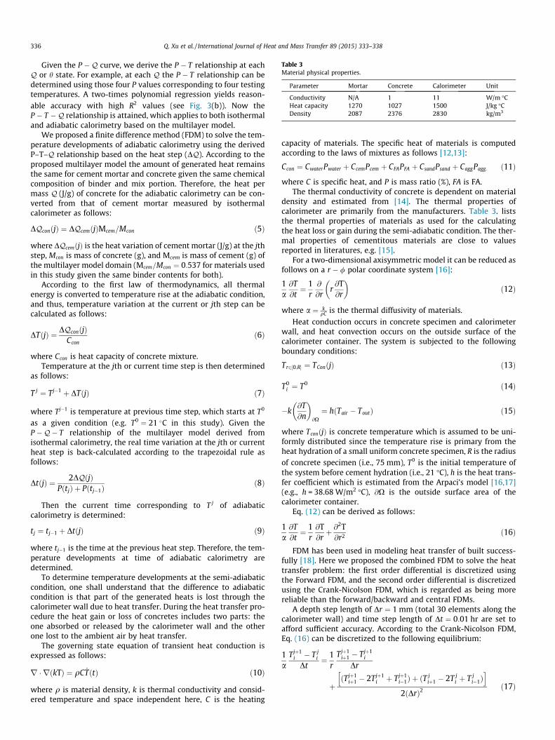
Table 3Material physical properties.

Parameter Mortar Concrete Calorimeter Unit

Conductivity N/A 1 11 W/m �CHeat capacity 1270 1027 1500 J/kg �CDensity 2087 2376 2830 kg/m3

336 Q. Xu et al. / International Journal of Heat and Mass Transfer 89 (2015) 333–338

Given the P �Q curve, we derive the P � T relationship at eachQ or h state. For example, at each Q the P � T relationship can bedetermined using those four P values corresponding to four testingtemperatures. A two-times polynomial regression yields reason-able accuracy with high R2 values (see Fig. 3(b)). Now theP � T �Q relationship is attained, which applies to both isothermaland adiabatic calorimetry based on the multilayer model.

We proposed a finite difference method (FDM) to solve the tem-perature developments of adiabatic calorimetry using the derivedP–T–Q relationship based on the heat step (DQ). According to theproposed multilayer model the amount of generated heat remainsthe same for cement mortar and concrete given the same chemicalcomposition of binder and mix portion. Therefore, the heat permass Q (J/g) of concrete for the adiabatic calorimetry can be con-verted from that of cement mortar measured by isothermalcalorimeter as follows:

DQconðjÞ ¼ DQcemðjÞMcem=Mcon ð5Þ

where DQcemðjÞ is the heat variation of cement mortar (J/g) at the jthstep, Mcon is mass of concrete (g), and Mcem is mass of cement (g) ofthe multilayer model domain (Mcem=Mcon ¼ 0:537 for materials usedin this study given the same binder contents for both).

According to the first law of thermodynamics, all thermalenergy is converted to temperature rise at the adiabatic condition,and thus, temperature variation at the current or jth step can becalculated as follows:

DTðjÞ ¼ DQconðjÞCcon

ð6Þ

where Ccon is heat capacity of concrete mixture.Temperature at the jth or current time step is then determined

as follows:

T j ¼ Tj�1 þ DTðjÞ ð7Þ

where Tj�1 is temperature at previous time step, which starts at T0

as a given condition (e.g. T0 ¼ 21 �C in this study). Given theP �Q� T relationship of the multilayer model derived fromisothermal calorimetry, the real time variation at the jth or currentheat step is back-calculated according to the trapezoidal rule asfollows:

DtðjÞ ¼ 2DQðjÞPðtjÞ þ Pðtj�1Þ

ð8Þ

Then the current time corresponding to T j of adiabaticcalorimetry is determined:

tj ¼ tj�1 þ DtðjÞ ð9Þ

where tj�1 is the time at the previous heat step. Therefore, the tem-perature developments at time of adiabatic calorimetry aredetermined.

To determine temperature developments at the semi-adiabaticcondition, one shall understand that the difference to adiabaticcondition is that part of the generated heats is lost through thecalorimeter wall due to heat transfer. During the heat transfer pro-cedure the heat gain or loss of concretes includes two parts: theone absorbed or released by the calorimeter wall and the otherone lost to the ambient air by heat transfer.

The governing state equation of transient heat conduction isexpressed as follows:

r � rðkTÞ ¼ qC _TðtÞ ð10Þ

where q is material density, k is thermal conductivity and consid-ered temperature and space independent here, C is the heating

capacity of materials. The specific heat of materials is computedaccording to the laws of mixtures as follows [12,13]:

Ccon ¼ CwaterPwater þ CcemPcem þ CFAPFA þ CsandPsand þ CaggPagg: ð11Þ

where C is specific heat, and P is mass ratio (%), FA is FA.The thermal conductivity of concrete is dependent on material

density and estimated from [14]. The thermal properties ofcalorimeter are primarily from the manufacturers. Table 3. liststhe thermal properties of materials as used for the calculatingthe heat loss or gain during the semi-adiabatic condition. The ther-mal properties of cementitous materials are close to valuesreported in literatures, e.g. [15].

For a two-dimensional axisymmetric model it can be reduced asfollows on a r � / polar coordinate system [16]:

1a@T@t¼ 1

r@

@rr@T@r

� �ð12Þ

where a ¼ kqC is the thermal diffusivity of materials.

Heat conduction occurs in concrete specimen and calorimeterwall, and heat convection occurs on the outside surface of thecalorimeter container. The system is subjected to the followingboundary conditions:

Tr2½0;R� ¼ TConðjÞ ð13Þ

T0i ¼ T0 ð14Þ

�k@T@n

� �@X

¼ hðTair � ToutÞ ð15Þ

where TconðjÞ is concrete temperature which is assumed to be uni-formly distributed since the temperature rise is primary from theheat hydration of a small uniform concrete specimen, R is the radiusof concrete specimen (i.e., 75 mm), T0 is the initial temperature ofthe system before cement hydration (i.e., 21 �C), h is the heat trans-fer coefficient which is estimated from the Arpaci’s model [16,17](e.g., h = 38.68 W/m2 �C), @X is the outside surface area of thecalorimeter container.

Eq. (12) can be derived as follows:

1a@T@t¼ 1

r@T@rþ @

2T@r2 ð16Þ

FDM has been used in modeling heat transfer of built success-fully [18]. Here we proposed the combined FDM to solve the heattransfer problem: the first order differential is discretized usingthe Forward FDM, and the second order differential is discretizedusing the Crank-Nicolson FDM, which is regarded as being morereliable than the forward/backward and central FDMs.

A depth step length of Dr ¼ 1 mm (total 30 elements along thecalorimeter wall) and time step length of Dt ¼ 0:01 hr are set toafford sufficient accuracy. According to the Crank-Nicolson FDM,Eq. (16) can be discretized to the following equilibrium:

1a

Tjþ1i � T j

i

Dt¼ 1

rTjþ1

iþ1 � Tjþ1i

Dr

þðTjþ1

iþ1 � 2Tjþ1i þ Tjþ1

i�1Þ þ ðTjiþ1 � 2T j

i þ T ji�1Þ

h i

2ðDrÞ2ð17Þ

Estimated from measurementsModeled

Fig. 4. Calculated temperature losses versus measurement estimations.

20

22

24

26

28

30

32

34

36

38

40

0 20 40 60 80 100 120 140 160 18020

30

40

50

60

70

80

90

100

Sem

i-adi

aba�

c te

mpe

ratu

re (o C

)

Time (hr)

Adi

aba�

c te

mpe

ratu

re (o C

)

Simula�ons

Measurements

Adiabatic

Semi-adiabatic

Air temperature

Fig. 5. Simulated adiabatic and semi-adiabatic temperatures versus measurements(along with measured air temperature).

Q. Xu et al. / International Journal of Heat and Mass Transfer 89 (2015) 333–338 337

where T ji is temperature at the ith element and jth time step for

i ¼ 1;2 . . . m (total m elements and mþ 1 nodes including the start-ing node with an ID of ‘‘0’’) and j ¼ 0;1;2 . . . n� 1 (total n time stepsand nþ 1 time points including zero time). Eq. (17) can bere-arranged as follows:

� 12Dr2 þ

1rDr

� �Tjþ1

iþ1 þ1

aDtþ 1

rDrþ 1

Dr2

� �Tjþ1

i � 12Dr2 Tjþ1

i�1

¼T j

iþ1

2Dr2 þ1

aDt� 1

Dr2

� �T j

i þT j

i�1

2Dr2 ð18Þ

This formula can be re-expressed in a matrix–vector linear sys-tem as follows:

K½Tjþ1m Tjþ1

m�1 . . . Tjþ11 Tjþ1

0 �T¼ A½T j

mT jm�1 . . . T j

1T j0�

Tð19Þ

where the vector on the left and right represents the temperatureprofile at the (j + 1)th and jth time step, respectively, K is the stiff-ness matrix, and A is a parameter matrix such that:

Kij ¼

� 12Dr2 þ 1

rDr

� �i ¼ j

1aDt þ 1

rDr þ 1Dr2

� �j ¼ iþ 1

� 12Dr2 j ¼ iþ 2

0 others

8>>>><>>>>:

ð20Þ

Aij ¼

12Dr2 i ¼ j

1aDt � 1

Dr2

� �i ¼ j� 1

12Dr2 i ¼ j� 20 others

8>>>>>><>>>>>>:

ð21Þ

Since K is positive definite, the temperature profile at the(j + 1)th time step can be solved as follows from Eq. (19):

½Tjþ1m Tjþ1

m�1 . . . Tjþ11 Tjþ1

0 �T¼ ðKT KÞ�1

KT A½T jmT j

m�1 . . . T j1T j

0�T

ð22Þ

Given temperatures of the calorimeter wall, the absorbed orreleased heat (when P is small it releases the absorbed heat) ofthe calorimeter can be calculated as follows:

DQcalðjÞ ¼Z R2

R1

CcalDT jqH2prdr=Mcal ð23Þ

where Ccal is the heat capacity of calorimeter, DT j is temperaturevariation, R1 (150 mm) and R2 (180 mm) is the inner and exteriorradius of calorimeter, respectively, H is the height of the calorimeter(300 mm), q is density of calorimeter material, and Mcal is the massof calorimeter wall such that:

Mcal ¼Z R2

R1

qH2prdr ¼ pqHðR22 � R2

1Þ ð24Þ

After integration and discretization DQcalðjÞ can be approxi-mated as follows:

DQcalðjÞ ¼1

R22 � R2

1

Xi

ðr2i � r2

i�1ÞðDT ji þ DT j

i�1Þ=2 ð25Þ

The heat loss of concrete to the ambient air at the jth time stepis calculated as follows:

DQairðjÞ ¼ð2pR2HÞhðT j

air � T jmÞDt

Mconð26Þ

where 2pR2H is the exterior surface area (m2) of the semi-adiabaticcalorimeter wall, Dt is time step length (s), h is heat transfer coeffi-

cient (W/m2 �C), T jair is the temperature of air (�C), T j

m is the temper-ature of the outside surface of calorimeter, and Mcon is the mass ofconcrete (g). Therefore, the total temperature loss of cementitious

materials due to heat transfer and the absorption or release of thecalorimeter itself at the current time step can be calculated asfollows:

DTlossðjÞ ¼DQcalðjÞ þ DQairðjÞ

Cconð27Þ

Note that DTlossðjÞ can be positive (heat loss, mostly) or negative(heat gain). Thus, the temperature of semi-adiabatic calorimetry atthe current time step is determined as follows:

T j ¼ Tj�1 � DTlossðjÞ ð28Þ

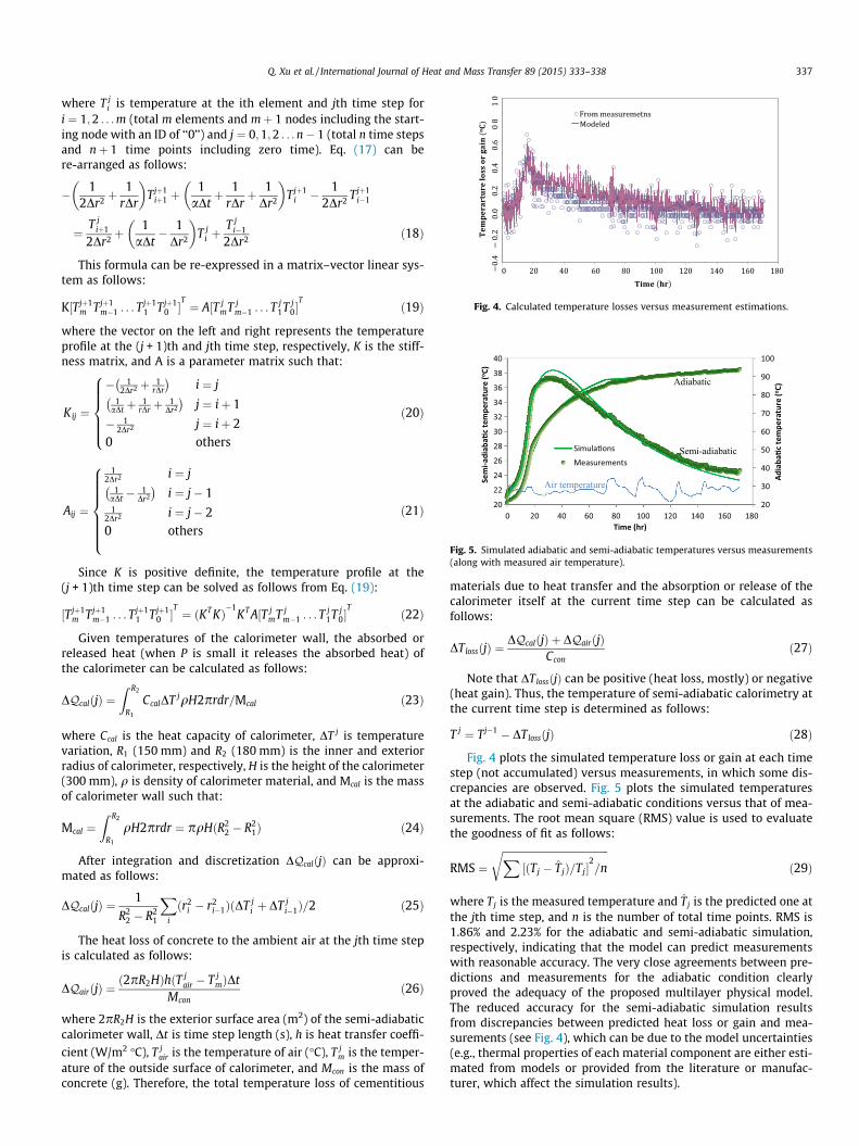
Fig. 4 plots the simulated temperature loss or gain at each timestep (not accumulated) versus measurements, in which some dis-crepancies are observed. Fig. 5 plots the simulated temperaturesat the adiabatic and semi-adiabatic conditions versus that of mea-surements. The root mean square (RMS) value is used to evaluatethe goodness of fit as follows:

RMS ¼ffiffiffiffiffiffiffiffiffiffiffiffiffiffiffiffiffiffiffiffiffiffiffiffiffiffiffiffiffiffiffiffiffiffiffiffiffiffiffiffiffiffiX½ðTj � T̂ jÞ=Tj�

2=n

rð29Þ

where Tj is the measured temperature and T̂ j is the predicted one atthe jth time step, and n is the number of total time points. RMS is1.86% and 2.23% for the adiabatic and semi-adiabatic simulation,respectively, indicating that the model can predict measurementswith reasonable accuracy. The very close agreements between pre-dictions and measurements for the adiabatic condition clearlyproved the adequacy of the proposed multilayer physical model.The reduced accuracy for the semi-adiabatic simulation resultsfrom discrepancies between predicted heat loss or gain and mea-surements (see Fig. 4), which can be due to the model uncertainties(e.g., thermal properties of each material component are either esti-mated from models or provided from the literature or manufac-turer, which affect the simulation results).

338 Q. Xu et al. / International Journal of Heat and Mass Transfer 89 (2015) 333–338

4. Conclusions

In the above-present study, we proposed a multilayer physicalmodel and mathematical solution to predict temperature develop-ments of the adiabatic and semi-adiabatic calorimetry from the mea-sured heat evolution of isothermal calorimetry. We also developed anumerical solution with implementations for cementitious materials.Using the proposed model and numerical solution, we properly pre-dicted the adiabatic and semi-adiabatic temperatures of concretespecimen from the isothermal calorimetry of cement mortar. Thisnewly developed model can also be applied to other materials in dif-ferent industries for calorimetry analysis to save engineering costsand improve efficiency in experimental work and equipment.

Conflict of interest

None declared.

Acknowledgements

This research is partially supported by the US Department ofTransportation, Federal Highway Administration (FHWA) project(FHWA DTFH-61-06-H-00011). We also appreciate valuable dis-cussions with Mr. Mauricio Ruiz at the Transtec Group, Inc. atthe early stage of model development, and the assistance of grad-uate students in laboratory tests at the National ConcretePavement Technology Center at the Iowa State University.

References

[1] N.Y. Mostafa, P.W. Brown, Heat of hydration of high reactive pozzolans inblended cements: Isothermal conduction calorimetry, Thermochim. Acta 435(2005) 162–167.

[2] S. Mindess, J.F. Young, Concrete, Prentice-Hall Inc, Englewood Cliffs, NJ, 1981.1981.

[3] Z. Sun, Q. Xu, Micromechanical analysis of polyacrylamide modified concretefor improving strengths, Mater. Sci. Eng. A 490 (2008) 181–192.

[4] Z. Sun, Q. Xu, Microscopic, physical and mechanical analysis of polypropylenefiber reinforced concrete, Mater. Sci. Eng. A 527 (2009) 198–204.

[5] J.L. Poole, K.A. Riding, K.J. Folliard, M.C.G. Juenger, A.K. Schindler, Hydrationstudy of cementitious materials using semi-adiabatic calorimetry, ACI Mater. J.241 (2007) 59–76.

[6] P.F. Hansen, E.J. Pedersen, Maturity computer for controlling. curing andhardening of concrete, Nordisk Betong 19 (1977) 21–25.

[7] Q. Xu, J. Hu, J.M. Ruiz, K. Wang, Z. Ge, Isothermal calorimetry tests andmodeling of cement hydration parameters, Thermochim. Acta 499 (2010) 91–99.

[8] L. Wadsö. An experimental comparison between isothermal calorimetry,semiadiabatic calorimetry and solution calorimetry for the study of cementhydration. Final report, ORDTEST Report TR522, 2002.

[9] Q. Xu, J.M. Ruiz, J. Hu, K. Wang, R. Rasmussen, Modeling hydration propertiesand temperature developments of early-age concrete pavement, Thermochim.Acta 512 (2011) 76–85.

[10] S.M. Monteagudo, A. Moragues, J.C. Gálvez, M.J. Casati, E. Reyes, The degree ofhydration assessment of blended cement pastes by differential thermal andthermogravimetric analysis. Morphological evolution of the solid phases,Thermochim. Acta 592 (2014) 37–51.

[11] A.K. Schindler, K.J. Folliard, Heat of hydration models for cementitiousmaterials, ACI Mater. J. 102 (2005) 24–33.

[12] P. Choktaweekarn, W. Saengsoy, S. Tangfermsirikul, A model for predicting thespecific heat capacity of fly-ash concrete, Sci. Asia 35 (2009) 178–182.

[13] D.P. Bentz, Transient plane source measurements of the thermal properties ofhydrating cement pastes, Mater. Struct. 40 (2007) 1073–1080.

[14] American Concrete Institute, Guide to thermal properties of concrete andmasonry systems. ACI 122R–02, 2002.

[15] D.P. Bentz1, M.A. Peltz, A. Durán-Herrera, P. Valdez, C.A. Juárez, Thermalproperties of high-volume FA mortars and concretes, J. Building Phys. 34(2011) 263–275.

[16] Q. Xu, M. Solaimanian, Modeling temperature distribution and thermalproperty of asphalt concrete for laboratory testing applications, Constr.Building Mater. 24 (2010) 487–497.

[17] S.V. Arpaci, S.H. Kao, A. Selamet, Introduction to heat transfer. New Jersey,1999.

[18] Y. Chen, A.K. Athienitis, K.E. Galal, Frequency domain and finite differencemodeling of ventilated concrete slabs and comparison with fieldmeasurements: Part 1, modeling methodology, Int. J. Heat Mass Transfer 66(2013) 948–956.