arX

iv:g

r-qc

/020

6072

v2 1

8 Ju

l 200

2

Gauge conditions for long-term numerical black hole evolutions without excision

Miguel Alcubierre(1,2), Bernd Brugmann(1), Peter Diener(1), Michael Koppitz(1), Denis Pollney(1),Edward Seidel(1,3), and Ryoji Takahashi(1,4)

(1) Max-Planck-Institut fur Gravitationsphysik, Albert-Einstein-Institut, Am Muhlenberg 1, 14476 Golm, Germany(2) Instituto de Ciencias Nucleares, Universidad Nacional Autonoma de Mexico, A.P. 70-543, 04510 Mexico, D. F., Mexico.

(3) National Center for Supercomputing Applications, Beckman Institute, 405 N. Mathews Ave., Urbana, IL 61801(4) Theoretical Astrophysics Center, Juliane Maries Vej 30, 2100 Copenhagen, Denmark

(June 25, 2002; AEI-2002-037)

Numerical relativity has faced the problem that standard 3+1 simulations of black hole spacetimeswithout singularity excision and with singularity avoiding lapse and vanishing shift fail after anevolution time of around 30 − 40M due to the so-called slice stretching. We discuss lapse and shiftconditions for the non-excision case that effectively cure slice stretching and allow run times of1000M and more.

04.25.Dm, 04.30.Db, 95.30.Sf, 97.60.Lf

I. INTRODUCTION

A crucial role in numerical relativity simulations oftwo black holes (BH) is played by the choice of coor-dinates. This gauge choice involves both the choice ofa lapse function and of a shift vector, which typicallyhave to be determined dynamically during a numericalevolution. The first results for colliding BH’s were ob-tained for head-on collisions using the ADM decomposi-tion of the Einstein equations with the lapse determinedby the maximal slicing condition and the shift vector setto zero [1–3]. Maximal slices are known to be singular-ity avoiding, that is, starting from BH initial data wherethe physical singularity is to the future of the initial hy-persurface, the lapse approaches the Minkowski value ofunity in the asymptotically flat regions, but approacheszero near the physical singularity. In this way one canin principle foliate a BH spacetime without singularities,but since time marches on in the far regions while beingfrozen in the interior, the slices become more and moredistorted. Historically, this phenomenon has been called‘grid stretching’ by the numerical relativity community,though we will refer to it as ‘slice stretching’ since it isa property of the slices themselves, quite independent ofthe existence of a numerical grid. Slice stretching intro-duces a difficult problem for numerical simulations sincethe metric develops large gradients that keep on growinguntil the numerical code can no longer handle them andfails. Advanced numerical methods can help in sphericalsymmetry, see, e.g., [4], but to date have not proved verysuccessful in three-dimensional (3D) evolutions [5].

Nonetheless, such singularity avoiding slicings withvanishing shift have been quite successful, since they doallow a finite evolution time of roughly t = 30 − 40M(with M the total ADM mass of the system) for fully3D evolutions of BH’s, as first demonstrated in 1995 forthe case of a single Schwarzschild BH [6]. In [7] the firstfully 3D simulation of the grazing collision of two nearbyBH’s was performed with singularity avoiding slicing and

vanishing shift, lasting for about 7M . With improvedtechniques the grazing collision has recently been pushedto about 35M , which for the first time allowed the ex-traction of gravitational waveforms from a 3D numericalmerger [8]. And even though singularity avoiding slic-ings with vanishing shift have so far been limited to afinite time interval of only 30 − 40M , this interval canbe moved into the truly non-linear regime of a plungestarting from an approximate innermost stable circularorbit (ISCO) of two BH’s, since the remainder of themerger and ring-down can be computed using the closelimit approximation [9]. Following such an approach, thefirst waveforms for the plunge from an approximate ISCOhave been obtained [10–12].

So far the most important strategy to avoid slicestretching has been black hole excision [13,14]. The ideais to use horizon penetrating coordinates (notice thatmaximal slicing is horizon penetrating unless one imposesthe extra boundary condition of having a vanishing lapseat the horizon) and to excise the interior of the BH’s fromthe numerical grid. A non-vanishing shift is essential tokeep grid points from falling into the BH. This approachhas seen many successful implementations for single blackholes. First demonstrated in 3D in [6], with further de-velopment it has, in particular, allowed to move a blackhole across the numerical grid [15]. If a stable numericalimplementation can be found, this approach should makeit possible to simulate many orbits of two well separatedBH’s. The key difference between BH excision and theuse of singularity avoiding slicings with vanishing shift isthat with excision single static BH’s can be stably evolvedfor thousands of M ; see [15] for the case of evolutions us-ing null coordinates (that do not directly generalize tobinary BH systems), and recently 100, 000M have beenreached for a single BH with a 3+1 Cauchy code in oc-tant symmetry [16]. Black hole excision holds a lot ofpromise, even if currently evolutions of only 9–15M havebeen achieved for binary BH’s [17].

In this paper we demonstrate that the new lapse and

1

shift conditions introduced in [18] for the case of a singledistorted BH with excision (using the excision techniquesof [16]) can work well even without excision. This allowsus to break through the barrier of about 35M for singu-larity avoiding slicings in 3+1 numerical relativity. Ourgauge choice maintains singularity avoidance but curesthe main problems associated with slice stretching, al-lowing us to reach 500M and more for the evolution ofsingle or even distorted BH’s. For BH’s colliding head-on that merge early on during the evolution, i.e. whichstart out sufficiently close to each other, the final BH canagain be evolved for hundreds or even thousands of M .

Moreover, these gauge conditions have two impor-tant effects: (a) they drive the system towards a staticstate, virtually, if not completely, eliminating the chronicgrowth in metric functions typical of slice stretching.Hence, in principle they should allow for indefinitely longevolutions (if no other instabilities develop; see below).(b) since unbounded growth in metric functions is halted,they allow much more accurate results to be obtained forextremely long times, and at lower resolution than be-fore. Below we will show results obtained for collidingblack holes that show only 10% error in the horizon massafter more than 5000M of evolution.

The evolutions in this paper are carried out using thepuncture method for evolutions [7,6]. The starting pointis initial data of the Brill-Lindquist topology in isotropiccoordinates [19]. This ‘puncture’ data is defined on R3

minus a point for each of the internal asymptotically flatends of the BH’s. If one treats the coordinate singular-ity at the punctures appropriately, the punctures do notevolve as long as the shift vanishes there. That is, themetric and the extrinsic curvature do not evolve at thepunctures. It can also be checked that the maximal slic-ing equation produces a smooth numerical solution forthe lapse at the punctures.

One basic observation for our choice of shift vector isthat the “Gamma freezing” shift introduced in [18] forour project in simple BH excision has the following prop-erty when the BH’s are not excised but are representedas punctures: Initially the shift is zero, but as the slicestretching develops, the shift reacts by pulling out pointsfrom the inner asymptotically flat region near the punc-tures. The lapse and shift conditions taken together arethen able to virtually stop the evolution of one or eventwo black holes, essentially mimicking the behavior of thelapse and shift known from stable evolutions of a BH inKerr-Schild coordinates. This is a key result that will bedetailed below.

The paper is organized as follows. First we introducethe evolution equations and the constraints in Section II.In Sec. III we discuss the gauge conditions. The punc-ture initial data and puncture evolutions are discussed inSec. IV and Sec. V. In Sec. VI miscellaneous aspects ofour numerical implementation are discussed. In Sec. VIIwe present numerical results for one and two BH’s, andwe conclude in Sec. VIII.

II. FORMULATION

The standard variables in the 3+1 formulation of ADM(Arnowitt-Deser-Misner, see [20]) are the 3-metric γijand the extrinsic curvatureKij . The gauge is determinedby the lapse function α and the shift vector βi. We willonly consider the vacuum case. The evolution equationsare

(∂t − Lβ) γij = −2αKij , (1)

(∂t − Lβ) Kij = −DiDjα

+α(Rij +KKij − 2KikKkj), (2)

and the constraints are

H ≡ R+K2 −KijKij = 0, (3)

Di ≡ Dj(Kij − γijK) = 0. (4)

Here Lβ is the Lie derivative with respect to the shift vec-tor βi, Di is the covariant derivative associated with the3-metric γij , Rij is the three-dimensional Ricci tensor, Rthe Ricci scalar, and K is the trace of Kij .

We will use the BSSN form of these equations (Baum-garte, Shapiro [21], and Shibata, Nakamura [22]). Oneintroduces new variables based on a trace decompositionof the extrinsic curvature and a conformal rescaling ofboth the metric and the extrinsic curvature. The trace-free part Aij of the extrinsic curvature is defined by

Aij = Kij −1

3γijK. (5)

Assuming that the metric γij is obtained from a confor-mal metric γij by a conformal transformation,

γij = ψ4γij , (6)

we can choose a conformal factor ψ such that the deter-minant of γij is 1:

ψ = γ1/12, (7)

γij = ψ−4γij = γ−1/3γij , (8)

γ = 1, (9)

where γ is the determinant of γij and γ is the determinantof γij . Instead of γij and Kij we can therefore use thevariables

φ = lnψ =1

12ln γ, (10)

K = γijKij , (11)

γij = e−4φγij , (12)

Aij = e−4φAij , (13)

where γij has determinant 1 and Aij has vanishingtrace. Furthermore, we introduce the conformal connec-tion functions

2

Γi = γjkΓijk = −∂j γij , (14)

where Γijk is the Christoffel symbol of the conformalmetric and where the second equality holds only if thedeterminant of the conformal 3-metric γ is unity (whichis true analytically but may not hold numerically). We

call φ, K, γij , Aij , and Γi the BSSN variables.In terms of the BSSN variables the evolution equation

(1) becomes

(∂t − Lβ) γij = −2αAij , (15)

(∂t − Lβ) φ = −1

6αK, (16)

while equation (2) leads to

(∂t − Lβ) Aij = e−4φ[−DiDjα+ αRij ]TF

+ α(KAij − 2AikAkj), (17)

(∂t − Lβ) K = −DiDiα

+ α(Aij Aij +

1

3K2), (18)

where TF denotes the trace-free part of the expressionin brackets with respect to γij . Note that the right-hand side of the evolution equation (17) for the trace-

free variable Aij is trace-free except for the term AikAkj .

This is no contradiction since the condition that Aijremains trace-free is (∂t − Lβ) (γijAij) = 0 and not

γij(∂t − Lβ) Aij = 0.On the right-hand side of (18) we have used the Hamil-

tonian constraint (3) to eliminate the Ricci scalar,

R = KijKij −K2 = AijA

ij − 2

3K2. (19)

The momentum constraint (4) becomes

∂jAij = −ΓijkA

jk − 6Aij∂jφ+2

3γij∂jK. (20)

An evolution equation for Γi can be obtained from (14)and (15),

∂tΓi = −2

(

α∂jAij + Aij∂jα

)

− ∂j(

Lβ γij)

, (21)

where we will use the momentum constraint above tosubstitute for the divergence of Aij . One subtlety inobtaining numerically stable evolutions with the BSSNvariables is precisely the question of how the constraintsare used in the evolution equations. Several choices arepossible and have been studied, see e.g. [23].

Note that in the preceding equations we are computingLie derivatives of tensor densities. If the weight of atensor density T is w, i.e. if T is a tensor times γw/2,then

LβT = [LβT ]w=0∂ + wT∂kβ

k, (22)

where the first term denotes the tensor formula for Liederivatives with the derivative operator ∂ and the secondis the additional contribution due to the density factor.The density weight of ψ = eφ is 1

6 , so the weight of γijand Aij is − 2

3 and the weight of γij is 23 . To be explicit,

Lβφ = βk∂kφ+1

6∂kβ

k, (23)

Lβ γij = βk∂kγij + γik∂jβk + γjk∂iβ

k − 2

3γij∂kβ

k, (24)

Lβ γij = βk∂kγij − γik∂kβ

j − γjk∂kβi +

2

3γij∂kβ

k. (25)

The evolution equation (21) for Γi therefore becomes

∂tΓi = γjk∂j∂kβ

i +1

3γij∂j∂kβ

k

+βj∂jΓi − Γj∂jβ

i +2

3Γi∂jβ

j

−2Aij∂jα+ 2α(ΓijkAjk + 6Aij∂jφ− 2

3γij∂jK).

(26)

In the second line we see the formula for a vector densityof weight 2

3 , but since Γi is not really a tensor densitybut is derived from Christoffel symbols we obtain extraterms involving second derivatives of the shift (the firstline in the equation above).

On the right-hand sides of the evolution equations forAij and K, (17) and (18), there occur covariant deriva-tives of the lapse function, and the Ricci tensor of thenon-conformal metric. Since

Γkij = Γkij + 2(δki ∂jφ+ δkj ∂iφ− γij γkl∂lφ), (27)

where Γkij is the Christoffel symbol of the conformal met-ric, we have for example

DiDiα = e−4φ(γij∂i∂jα− Γk∂kα+ 2γij∂iφ∂jα). (28)

The Ricci tensor can be separated in two parts,

Rij = Rij +Rφij , (29)

where Rij is the Ricci tensor of the conformal metric and

Rφij denotes additional terms depending on φ:

Rφij = −2DiDjφ− 2γijDkDkφ

+4Diφ Djφ− 4γijDkφ Dkφ, (30)

with Di the covariant derivative associated with the con-formal metric. The conformal Ricci tensor can be writtenin terms of the conformal connection functions as

Rij = −1

2γlm∂l∂mγij + γk(i∂j)Γ

k + ΓkΓ(ij)k

+γlm(

2Γkl(iΓj)km + ΓkimΓklj

)

. (31)

3

A key observation here is that if one introduces theΓi as independent variables, then the principal part ofthe right-hand side of equation (17) contains the waveoperator γlm∂l∂mγij but no other second derivatives ofthe conformal metric. This brings the evolution systemone step closer to being hyperbolic.

One of the reasons why we have written out the BSSNsystem in such detail is to point out a subtlety that arisesin the actual implementation if one wants to achieve nu-merical stability. In the computer code we do not use thenumerically evolved Γi in all places, but follow this rule:

• Partial derivatives ∂jΓi are computed as finite dif-

ferences of the independent variables Γi that areevolved using (26).

• In all expressions that just require Γi and not itsderivative we substitute γjkΓijk(γ), that is we do

not use the independently evolved variable Γi butrecompute Γi according to its definition (14) fromthe current values of γij .

In practice we have found that the evolutions are far lessstable if either Γi is treated as an independent variableeverywhere, or if Γi is recomputed from γij before eachtime step. The rule just stated helps to maintain theconstraint Γi = −∂j γij well behaved without removingthe advantage of reformulating the principal part of theRicci tensor.

In summary, we evolve the BSSN variables γij , φ, Aij ,

K, and Γi according to (15), (16), (17), (18), and (26), re-spectively. The Ricci tensor is separated as shown in (29)with each part computed according to (30) and (31) re-spectively. The Hamiltonian and momentum constraintshave been used to write the equations in a particular way.The evolved variables Γi are only used when their partialderivatives are needed (the one term in the conformal

Ricci tensor (31) and the advection term βk∂kΓi in the

evolution equation for the Γi themselves, Eq. (26)).

III. THE GAUGE CONDITIONS

We will consider families of gauge conditions that arenot restricted to puncture data and that can be used inprinciple with any 3+1 form of the Einstein’s equationsthat allows a general gauge. However, the specific fam-ily we test in this paper is best motivated by consideringthe BSSN system introduced above. For the present pur-poses, of special importance are the following two prop-erties of this formulation:

• The trace of the extrinsic curvature K is treatedas an independent variable. For a long time it hasbeen known that the evolution of K is directly re-lated to the choice of a lapse function α. Thus,having K as an independent field allows one to im-pose slicing conditions in a much cleaner way.

• The appearance of the “conformal connection func-tions” Γi as independent quantities. As al-ready noted by Baumgarte and Shapiro [21] (seealso [24,25]), the evolution equation for these quan-tities can be turned into an elliptic condition onthe shift which is related to the minimal distortioncondition. More generally, one can relate the shiftchoice to the evolution of these quantities, again al-lowing for a clean treatment of the shift condition.

Our aim is to look for gauge conditions that at latetimes, once the physical system under consideration hassettled to a final stationary state, will be able to drivethe coordinate system to a frame where this stationar-ity is evident. In effect, we are looking for “symme-try seeking” coordinates of the type discussed by Gund-lach and Garfinkle and also by Brady, Creighton, andThorne [26,27] that will be able to find the approximateKilling field that the system has at late times. In orderto achieve this we believe that the natural approach is torelate the gauge choice to the evolution of certain com-binations of dynamic quantities in such a way that thegauge will either freeze completely the evolution of thosequantities (typically by solving some elliptic equations),or will attempt to do so with some time delay (by solvinginstead parabolic or hyperbolic equations).

We will consider the lapse and shift conditions in turn.Special cases of the gauge conditions that we will intro-duce here were recently used together with BH excisionwith remarkable results in [16], but as we will show below,the conditions are so powerful that in the cases tested,they work even without excision.

A. Slicing conditions

The starting point for our slicing conditions is the “K-freezing” condition ∂tK=0, which in the particular casewhen K=0 reduces to the well known “maximal slicing”condition. The K-freezing condition leads to the follow-ing elliptic equation for the lapse:

∆α = βi∂iK + αKijKij , (32)

with ∆ the Laplacian operator for the spatial metric γij .In the BSSN formulation, once we have solved the ellipticequation for the lapse, the K-freezing condition can beimposed at the analytic level by simply not evolving K.

One can construct parabolic or hyperbolic slicing con-ditions by making either ∂tα or ∂2

t α proportional to ∂tK.We call such conditions “K-driver” conditions (see [28]).The hyperbolic K-driver condition has the form [4,18]

∂tα = −α2f(α)(K −K0), (33)

where f(α) is an arbitrary positive function of α andK0 = K(t = 0). In our evolutions, we normally take

f(α) =2

α, (34)

4

which is referred to as 1+log slicing, since empiricallywe have found that such a choice has excellent singu-larity avoiding properties. In Sec. IVB we introduce amodification of f(α) for puncture evolutions. The hyper-bolic K-driver condition is in fact only a slight general-ization of the Bona-Masso family of slicing conditions [4]:∂tα = −α2f(α)K.

By taking an extra time derivative of the slicing condi-tion above, and using the evolution equation for K, onecan see that the lapse obeys a generalized wave equation,

∂2t α = −∂t(α2f)(K −K0) − α2f∂tK

= α2f(∆α− αKijKij − βiDiK + 2αf + α2f ′). (35)

Previously we have also experimented with a somewhatdifferent form of hyperbolic K-driver condition

∂2t α = −α2f∂tK, (36)

where the right hand side vanishes in the case that Kfreezing is achieved. However, one may anticipate theproblem that even in the case when ∂tK = 0 we onlyobtain ∂tα = const, while for (33) we see that K = K0

implies that ∂tα = 0. Moreover, in black hole evolutionswhere the lapse collapses to zero, condition (33) guaran-tees that the lapse will stop evolving, while condition (36)only implies that ∂tα will stop evolving so the lapse caneasily “collapse” beyond zero and become negative. Forthese reasons, in practice the condition Eq. (33) leads tomore stable black hole evolutions, and this is the slicingcondition that we consider in this paper.

The wave speed in both cases is vα = α√

f(α), whichexplains the need for f(α) to be positive. Notice that,depending on the value of f(α), this wave speed can belarger or smaller than the physical speed of light. Thisrepresents no problem, as it only indicates the speed ofpropagation of the coordinate system, i.e. it is only a“gauge speed”. In particular, for the 1+log slicing in-troduced above with f = 2/α, the gauge speed in the

asymptotic regions (where α ≃ 1) becomes vα =√

2 > 1.One could then argue that choosing f = 1/α should be abetter alternative, as the asymptotic gauge speed wouldthen be equal to the physical speed of light. However,experience has shown that such a choice is not nearly asrobust and seems to lead easily to gauge pathologies asthose studied in [29,30].

B. Shift conditions

In the BSSN formulation, an elliptic shift condition iseasily obtained by imposing the “Gamma-freezing” con-dition ∂tΓ

k=0, or using (26),

γjk∂j∂kβi +

1

3γij∂j∂kβ

k − Γj∂jβi +

2

3Γi∂jβ

j + βj∂jΓi

−2Aij∂jα− 2α

(

2

3γij∂jK − 6Aij∂jφ− ΓijkA

jk

)

= 0.

(37)

Notice that, just as it happened with the K-freezing con-dition for the lapse, once we have solved the previouselliptic equations for the shift, the Gamma-freezing con-dition can be enforced at an analytic level by simply notevolving the Γk.

The Gamma-freezing condition is closely related to thewell known minimal distortion shift condition [31]. Inorder to see exactly how these two shift conditions arerelated, we write here the minimal distortion condition

∇jΣij = 0 , (38)

where Σij is the so-called “distortion tensor” defined as

Σij :=1

2γ1/3∂tγij , (39)

with γij the same as before. A little algebra shows thatthe evolution equation for the conformal connection func-tions (26) can be written in terms of Σij as

∂tΓi = 2∂j

(

γ1/3Σij)

. (40)

More explicitly, we have

∂tΓi = 2e4φ

[

∇jΣij − ΓijkΣ

jk − 6Σij∂jφ]

. (41)

We then see that the minimal distortion condition∇jΣij = 0, and the Gamma-freezing condition ∂tΓ

i = 0are equivalent up to terms involving first spatial deriva-tives of the spatial metric multiplied with the distortiontensor itself. In particular, all terms involving secondderivatives of the shift are identical in both cases (but notso terms with first derivatives of the shift which appearin the distortion tensor Σij). That the difference betweenboth conditions involves Christoffel symbols should notbe surprising since the minimal distortion condition iscovariant while the Gamma-freezing condition is not.

Just as it is the case with the lapse, we obtain parabolicand hyperbolic shift prescriptions by making either ∂tβ

i

or ∂2t β

i proportional to ∂tΓi. We call such conditions

“Gamma-driver” conditions. The parabolic Gammadriver condition has the form

∂tβi = Fp ∂tΓ

i , (42)

where Fp is a positive function of space and time. Inanalogy to the discussion of the hyperbolic K-driver con-dition there are two types of hyperbolic Gamma-driverconditions that we have considered,

∂2t β

i = F ∂tΓi − η ∂tβ

i, (43)

or alternatively,

∂2t β

i = F ∂tΓi − (η − ∂tF

F) ∂tβ

i, (44)

where F and η are positive functions of space and time.For the hyperbolic Gamma-driver conditions we have

5

found it crucial to add a dissipation term with coefficientη to avoid strong oscillations in the shift. Experience hasshown that by tuning the value of this dissipation coef-ficient we can manage to almost freeze the evolution ofthe system at late times.

The rational behind the two almost identical choicesof Gamma-driver is the following. First note that if F isindependent of time, the two choices are identical. How-ever, we typically choose F to be proportional to αp,with p some positive power (usually p = 1). Anticipatinga collapsing lapse near the black hole this implies thatthe term F∂tΓ

i approaches zero and the evolution of theshift tends to freeze independent of the behaviour andnumerical errors of ∂tΓ

i. We implement the first choiceof the Gamma-driver, (43), as

∂tβi = Bi, ∂tB

i = F∂tΓi − ηBi, (45)

and the second choice, (44), as

∂tβi = FBi, ∂tB

i = ∂tΓi − ηBi. (46)

The second variant has the advantage that if F ap-proaches zero due to the collapse of the lapse near ablack hole, then ∂tβ

i also approaches zero and the shiftfreezes. With the first variant, on the other hand, it isonly ∂tB

i = ∂2t β

i the one that approaches zero, whichmeans the shift can still evolve. Both Gamma-driverscan give stable black hole evolutions, although the sec-ond one leads to less evolution near the black holes.

An important point that needs to be considered whenusing the hyperbolic Gamma-driver condition is that ofthe gauge speeds. Just as it happened with the lapse,the use of a hyperbolic equation for the shift introducesnew “gauge speeds” associated with the propagation ofthe shift. In order to get an idea of how these gaugespeeds behave, we will consider for a moment the shiftcondition (43) for small perturbations of flat space (and

taking η=0). From the form of ∂tΓi given by equation

(26) we see that in such a limit the principal part of theevolution equation for the shift reduces to

∂2t β

i = F

(

δjk∂j∂kβi +

1

3δij∂j∂kβ

k

)

. (47)

Consider now only derivatives in a given direction, sayx. We find

∂2t β

i = F

(

∂2xβ

i +1

3δix∂x∂xβ

x

)

, (48)

which implies

∂2t β

x =4

3F∂2

xβx , (49)

∂2t β

q = F∂2xβ

q q 6= x . (50)

We can then see that in regions where the spacetimeis almost flat, the longitudinal part of the shift propa-gates with speed vlong = 2

√

F/3 while the transverse

part propagates with speed vtrans =√F . We therefore

choose

F (α) =3

4α, (51)

in order to have the longitudinal part of the shift prop-agate with the speed of light. The transverse part willpropagate at a different speed, but its contribution faraway is typically very small.

In the next section we will turn to puncture evolutions.Both f(α) and F (α) will be further adjusted for the pres-ence of punctures.

IV. PUNCTURES

So far our discussion of the BSSN formulation and theproposed gauge conditions was quite independent of anyparticular choice of initial data, except that our gaugeconditions are tailored for the late time stationarity ofbinary black hole mergers even though they are also ap-plicable in more general situations. In this Section weintroduce puncture initial data for black holes and themethod of puncture evolutions.

A. Puncture initial data

Consider the three-manifold R3 with one or morepoints (xA, yA, zA) removed. These points we call punc-tures. The punctured R3 arises naturally in solutionsto the constraints in the Lichnerowicz-York conformalmethod [32,20] for the construction of black hole initialdata. In the conformal method, we introduce on the ini-tial hypersurface at t = 0 the conformal variables γij andAij by

γij = ψ40 γij , (52)

Aij = ψ−20 Aij , (53)

where ψ0 is the conformal factor, and leave K untrans-formed. Note that Aij = ψ−6

0 Aij at t = 0.Consider initial data with the conformally flat metric

γij = ψ40δij . (54)

Assuming that the extrinsic curvature Kij vanishes, themomentum constraints (4) are trivially satisfied and theHamiltonian constraint (3) reduces to

∆δψ0 = 0, (55)

where ∆δ is the flat space Laplacian. A particular solu-tion to this equation is

ψ0 = 1 +m

2r, (56)

where r2 = x2 + y2 + z2 and we assume r 6= 0. This waywe have obtained initial data representing a slice of a

6

Schwarzschild black hole of mass m in spatially isotropiccoordinates on a punctured R3. The horizon is located atr = m/2. There are two asymptotically flat regions, onefor r → ∞ and a second one at r → 0. In fact, the metricis isometric under r′ = m2/(4r). Since (55) is linear inψ0 one immediately obtains solutions for multiple blackholes, for example

ψBL = 1 +m1

2r1+m2

2r2, (57)

where r2A = (x− xA)2 + (y − yA)2 + (z − zA)2 on an R3

with two punctures at (xA, yA, zA), A = 1, 2. These so-lutions were first mentioned in [33] and studied in detailby Brill and Lindquist in [19]. While no longer isometric,this initial data contains one or two black holes depend-ing on the separation of the punctures, but in any casewith two separate inner asymptotic regions at the punc-tures. In particular, there is no physical singularity atthe punctures, but there is a coordinate singularity ateach puncture if one considers the unpunctured R3.

Brill-Lindquist data can be generalized to longitudinal,non-vanishing extrinsic curvature Kij for multiple blackholes with linear momentum and spin [34,35]. Here oneuses the Bowen-York extrinsic curvature,

Aij =3

2r2(niP j + njP i − (δij − ninj))δkln

kP l)

+3

r3(niǫjklSknl + njǫiklSknl), (58)

and K = 0. The parameters P i and Si are the linear andangular ADM momentum, and ni = xi/r is the coordi-nate normal vector. The sum of two Bowen-York termscentered at two punctures is an explicit solution to theconformal momentum constraint with K = 0.

The key observation for puncture initial data is that,even though there is a coordinate singularity at eachpuncture, both in the conformal factor and in the Bowen-York extrinsic curvature, we can rewrite the Hamiltonianconstraint as a regular equation on R3 without any punc-ture points removed. This equation possesses a uniquesolution u that is C2 at the punctures and C∞ elsewhere,and the original Hamiltonian constraint is solved by

ψ0 = u+ ψBL. (59)

Working on R3 simplifies the numerical solution of theconstraints over methods that for example use an isome-try condition at the throat of a black hole.

Note that the puncture method for initial data can beapplied using a conformally flat metric and the Kerr ex-trinsic curvature [36], and also to non-conformally flatinitial data for multiple Kerr black holes [37–39]. In thispaper we restrict ourselves to the conformally flat punc-ture data with Bowen-York extrinsic curvature.

B. Puncture evolutions in the ADM system

In this section we want to argue that one can obtainregular evolutions of puncture initial data without re-moving a region containing the puncture coordinate sin-gularity from the grid by, say, an isometry condition atthe throat of the black holes as in [3], or through blackhole excision [13,14]. Evolving on R3 instead of on R3

with a sphere removed and an additional boundary con-dition imposed results in a significant technical simplifi-cation.

That this is possible was first noticed experimentallyfor a single Schwarzschild puncture in [6] for ADM evolu-tions with singularity avoiding slicing and vanishing shift.By turning off the isometry condition at the throat andcomputing everywhere including next to the puncture,the lapse equation can still be solved for a numericallysmooth lapse with vanishing first derivative at the punc-ture that collapses to zero at and around the punctureduring the evolution. The numerical grid in these simu-lations is staggered around the puncture points.

In [7], puncture evolutions are proposed as a generalmethod for the evolution of the conformally flat, lon-gitudinal extrinsic curvature data of orbiting and spin-ning black holes discussed in Sec. IVA. In particular,an argument is given that the punctures do not evolve

by construction. This is not a theorem about the regu-larity of the solutions, as is available for puncture initialdata [34,35], but it is consistent with the numerical re-sults.

The basic idea is to examine the evolution equationsand the gauge conditions at t = 0 in the limit of smalldistance to one of the punctures. For simplicity we moveone of the punctures onto the origin and consider thelimit r → 0.

In this Section we will give a detailed version of theargument of [7] for the ADM equations with maximalslicing and vanishing shift, and then discuss the BSSNequations in Sec. IVC. First note that for the punctureinitial data based on (58) and (59) we have ψBL = O(1/r)and u = O(1), and therefore at t = 0,

ψ0 = O(1/r), (60)

ψ−10 = O(r), (61)

γij = ψ40δij = O(1/r4), (62)

Kij = ψ−20 Aij = O(1/r). (63)

We therefore observe that the ADM equations (1) and (2)for the evolution of the metric and the extrinsic curvatureare singular at the punctures.

The basic construction in puncture evolutions is to fac-tor out the time-independent conformal factor ψBL (andnot ψ0) given by the initial data,

γij = ψ4BLγij , (64)

Kij = ψ4BLKij . (65)

7

The key difference to the BSSN rescaling is that punctureevolutions involve a special rescaling that is independentof time.

Eq. (64) gives rise to a method for accurate finite dif-ferencing of the metric. For example, for the first partialderivative we have

∂kγij = ψ4BL∂kγij + γij∂kψ

4BL, (66)

where ψ4BL and ∂kψ

4BL are given analytically, and γij and

∂kγij are assumed to remain regular during the evolution.By staggering the puncture between grid points one cantherefore still obtain accurate derivatives of γij near thepuncture, and this applies to all quantities derived fromthe metric and its derivatives like the Christoffels and theRicci tensor. In particular, there is no finite differencingacross the singularity of 1/r terms.

In general, we have ψ0 = u + ψBL and the analyticderivatives of ψ0 are not known, but we can still factorout ψBL as in (64) and (65) and obtain regular initialdata,

γij = ψ−4BLψ

40δij = O(1), (67)

Kij = ψ−4BLψ

−20 Aij = O(r3). (68)

The question is whether γij and Kij develop a singularityduring the course of the evolution.

The ADM equations for γij and Kij in the case ofvanishing shift are

∂tγij = −2αKij, (69)

∂tKij = ψ−4BL(−DiDjα+ αRij)

+γkl(KijKkl − 2KikKjl). (70)

Let us examine the terms on the right hand side of the∂tKij equation. For γij = O(1) and Kij = O(rn),

the terms involving Kij are of order O(r2n). Accord-

ing to (27), Γkij = Γkij + (ΓψBL)kij . Assuming that γij

and its derivatives are O(1), we have Γkij = O(1), but

(ΓψBL)kij = O(1/r). Hence Γkij = O(1/r), and simi-

larly Rij = O(1/r2). Finally, let us also assume thatthe lapse and its derivatives are of order O(1). Thenψ−4BLDiDjα = O(r3).With these assumptions we obtain for t = 0 that

∂tγij(0) = O(r3), (71)

∂tKij(0) = O(r2), (72)

where the O(r2) in the last equation is contributed bythe term involving the Ricci tensor, the lapse terms areO(r3), and the extrinsic curvature terms are O(r6). Inorder to study the time evolution, we can perform onefinite differencing step in time from t = 0 to t = ∆t, forexample,

γij(∆t) = γij(0) + ∆t∂tγij(0) = O(1), (73)

Kij(∆t) = Kij(0) + ∆t∂tKij(0) = O(r2). (74)

Note that Kij has dropped from O(r3) to O(r2). How-ever, it is readily checked that a second finite time stepdoes not further lower the order of any variable since theorder of the right hand side in the evolution equation ofKij is dominated by ψ−4

BLRij . We therefore find that

γij(t) = O(1), ∂tγij(t) = O(r2), (75)

Kij(t) = O(r2), ∂tKij(t) = O(r2). (76)

This argument suggests that if the lapse α and its deriva-tives do not introduce additional singularities at thepunctures, and if there are no singularities appearing inthe spatial derivatives of the metric (which we have notcompletely ruled out), then the right-hand sides of the

evolution equations for γij and Kij vanish at the punc-

tures for all times. This means that γij and Kij shouldnot evolve at all at the punctures for a regular slicing andvanishing shift by construction, and the same is true forgij and Kij .

C. Puncture evolutions in the BSSN system

For accurate finite differencing in the BSSN system forpuncture data we split the logarithmic conformal factorφ into a singular but time-independent piece and an ad-ditional time-dependent contribution χ,

φ = χ+ lnψBL. (77)

It remains to be seen whether χ and the remainingBSSN quantities are regular throughout the evolution,i.e. whether the coordinate singularity can be cleanly sep-arated out with ψBL as in the case of ADM. To decidethis issue we have to be specific about our gauge choice.In preparation for the discussion of the gauge for punc-ture evolutions in Sec. V we note some properties of theBSSN system near the punctures.

Each of the BSSN variables has the following initialvalue for puncture data at t = 0, which we assume toevolve as indicated by the arrows:

χ = O(1) → O(1), (78)

K = 0 → O(r2), (79)

γij = O(1) → O(1), (80)

Aij = O(r3) → O(r2), (81)

Γi = 0 → O(r). (82)

Assume furthermore that α = O(1), and that the deriva-tives of the O(1) quantities are O(1). Consider now thefollowing form of the evolution equations, where we haveinserted our assumptions for α, γij , Aij , and Γi, but havekept the explicit dependence on βi, φ and K:

∂tχ = Lβφ− 1

6αK, (83)

∂tK = LβK +O(r4)(O(1) +O(∂φ)) +1

3αK2, (84)

8

∂tγij = Lβ γij +O(r2), (85)

∂tAij = LβAij +KO(r2) +O(r4) (O(1)

+O(∂φ) +O(∂2φ) +O(∂φ)2)

, (86)

∂tΓi = −∂jLβ γij +O(r2) +O(r2)O(∂φ)

−4

3αγij∂jK. (87)

If these equations are to hold for all times, to be checkedby time stepping as in the last section, then we requirecertain assumptions about the shift as well. In particu-lar, each of the terms involving Lβ should be of the sameor higher order as the other terms in the correspondingequation, because otherwise there could be evolution to-wards lower orders in r. In particular, even assuming αand K are regular, we have to examine the behaviourof Lβφ at the puncture before we can conclude that χremains regular.

Let us assume that χ and its derivatives are regular,so that

φ = O(ln r), ∂iφ = O(1/r), ∂i∂jφ = O(1/r2). (88)

If furthermore K = O(r2), and if the shift terms areof sufficiently high order, then the right hand sides of(83)-(87) are at least O(r). In this case, the order ofeach equation is such that the corresponding orders in(78)-(82) are maintained. In Sec. V we show that theseassumptions can indeed be met by a proper gauge choice,and hence we arrive at the statement that in this case thepunctures do not evolve by construction.

V. GAUGE CONDITIONS AND PUNCTURE

EVOLUTIONS

The main question is whether there are lapse and shiftconditions that behave appropriately for puncture evolu-tions. We will show that this is indeed the case withoutthe need to introduce special boundary conditions at thepunctures. What is required is an appropriately regular-ized implementation of our gauge conditions and a choiceof initial data for lapse and shift such that the puncturesdo not evolve.

A. Lapse for puncture evolutions

Consider maximal slicing, which is implemented bychoosing K = 0 at t = 0 and determining the lapse fromthe elliptic equation resulting from ∂tK = 0, which forvanishing shift is

∆α = αKijKij . (89)

As discussed in [7], for gij = ψ4BLγij ,

∆α = ψ−4BL∆γα− δijΓkij∂kα, (90)

so the principal part is degenerating to zero as O(r4).To avoid numerical problems we therefore multiply (89)by ψ4

BL, which normalizes the principal part but leavesa O(1/r) term since Γkij = O(1/r):

∆γα−O(1/r)∂kα = O(r6)α. (91)

It turns out that standard numerical methods to solvethis elliptic equation will find a regular solution for α forwhich ∂kα vanishes sufficiently rapidly so that O(1/r)∂kαis zero at the puncture. Therefore, maximal slicing andvanishing shift lead to a sufficiently regular lapse suchthat indeed the right-hand sides of the ADM evolutionequations for γij and Kij vanish at the punctures.

Effectively, maximal slicing implements the conditionthat the lapse has a vanishing gradient at the puncture.Notice that this condition is very different to an isometry-type condition, where the lapse would be forced to be −1at the puncture. Fig. 1 shows a schematic representationin the Kruskal diagram of the type of slices one obtainsin the case of a single Schwarzschild BH when using threedifferent boundary conditions for the lapse (while keepingthe same interior slicing condition): odd at the throat,even at the throat and zero gradient at the puncture.When looking at these plots it is important to keep inmind that the puncture corresponds to a compactifica-tion of the second asymptotically flat region, and is atan infinite distance to the left of the plots. Notice that,in all three cases, far away on the right hand side of theplot the slices approach the Schwarzschild slices (in fact,if we use maximal slicing and ask for the lapse to be oddwe recover the Schwarzschild slices everywhere). Also, inthe case with an odd lapse the slices do not penetrate thehorizon, but in the other two cases they do.

Since maximal slicing is computationally expensive, weoften use 1+log slicing that mimics the behaviour of themaximal lapse in that it also is singularity avoiding andthe lapse drops to zero when the physical singularity ap-proaches. Analytically, however, the 1+log lapse doesnot necessarily drop to zero at the puncture. Startingwith α = 1 and K = 0 everywhere at t = 0, we see fromthe evolution equations for the lapse and for K,

∂tα = −α2f(α)(K −K0), (92)

∂tK = βi∂iK +1

3αK2 +O(r3), (93)

that neither α nor K evolve at the puncture if the shiftor the derivative of K vanishes at the puncture. Thatmeans that the lapse will remain 1 at the puncture, andthe inner asymptotically flat region will evolve. Numer-ically, one may expect this to be problematic if there isnot sufficient resolution, as will be normally the case. Thecode can become unstable near the puncture, and evenif it remains stable the event horizon may not preventnumerical inaccuracies to evolve into the outer regions.While this may happen, in practice the 1+log lapse doescollapse, apparently precisely because of a lack of resolu-tion, and the code remains stable. Even in this case we

9

FIG. 1. Schematic representation on the Kruskal diagramof the effect of the different boundary conditions on the slicesobtained. The first panel shows the case of an odd lapse atthe throat, the second panel the case of an even lapse at thethroat, and the last panel the case of a lapse with zero gradientat the puncture. The dashed lines show the singularities andthe dotted lines the event horizon.

typically obtain convergence in the outer regions wherethe lapse did not collapse.

In this paper we experiment with 1+log slicing withf(α) = 2/α replaced by f(α, ψBL) = 2ψmBL/α, so that

∂tα = −2αψmBL(K −K0), (94)

i.e. we have introduced a factor that for m > 0 can drivethe lapse to zero at the puncture. For m = 0 we ob-tain standard 1+log slicing. A natural choice is m = 4since then the singularity in ψ4

BL exactly matches the de-generacy of the principal part of the second order waveequation associated with the lapse evolution, see (35) and(90). In particular, for m = 4 the wave speed is regularat the puncture.

Both choices of 1+log slicing with initial lapse equal tounity have been found to lead to stable evolutions of blackholes with a lapse that satisfies the regularity conditionsassumed in the previous sections. Another approach toobtain a vanishing lapse at the puncture is to start witha different initial lapse, for example

α(t = 0) = ψ−2BL = O(r2), (95)

so that the lapse is zero at the puncture initially andthere is no evolution due to a non-vanishing lapse at thepuncture. The power −2 is chosen so that the initial lapsehas the same limit for r → ∞ as the lapse αisotropic =(1 − m

2r )/(1 + m2r ) of the static Schwarzschild metric in

isotropic coordinates. In practice, we have found thatwith such an initial lapse there sometimes is too much

evolution in the still poorly resolved region between thepuncture and the horizon, which is why we do not usethis option routinely. Instead of guessing an initial lapsethat minimizes the amount of initial evolution one shoulduse the lapse (and shift) derived from a quasi-equilibriumthin-sandwich puncture initial data set, which however iscurrently not available.

B. Shift for puncture evolutions

For long term stable evolutions, we want to constructa shift condition that counters slice-stretching. However,for arbitrary non-vanishing shift, equations (83-87) showthat the punctures will evolve. It is possible to havethe punctures move across the grid because of a non-vanishing shift. One problem would be the numericaltreatment of the coordinate singularity at the punctures,which so far was based on analytic derivatives of the time-independent conformal factor ψBL. While a solution ofthis problem may be possible, we focus here on finding ashift condition that counters slice-stretching while simul-taneously satisfying a fall-off condition for the shift suchthat the punctures do not evolve at all when using theBSSN equations.

As a first step it is instructive to consider βi = rni =xi = O(r) (with ni a radial unit vector) near the punc-ture. In this case several terms in the Lie derivativescancel exactly and we have

Lrnγij = xk∂kγij , (96)

LrnAij = xk∂kAij , (97)

LrnK = xk∂kK. (98)

However,

Lrnφ = xk∂kχ+ xk∂k lnψBL +1

2= O(1), (99)

so χ will evolve without a special combination of χ, K,and α. Furthermore, the Lie derivative will not be assimple if the shift is not exactly spherically symmetric.

We therefore turn to

βi = O(r3). (100)

This happens to be the necessary condition (assuminginteger powers of r) for the norm of the shift in the non-conformal metric to be zero at the puncture

γijβiβj = O(1/r4)δijβ

iβj . (101)

With βi = r3ni = r2xi we now have

Lr3nγij = O(r2)(xk∂kγij + γij) = O(r2), (102)

Lr3nφ = O(r2), (103)

All other Lie derivative terms also turn out to be of or-der O(r2). Finally, the shift derivatives in the evolution

equation for Γi are

10

∂jLβ γij = ∂jO(r2) = O(r). (104)

In this sense the evolution of Γi poses the strictest con-dition on the fall-off of the shift.

The question remains how we guarantee the O(r3) fall-off in the actual shift condition. We can enforce such afall-off by choosing

βi(t = 0) = 0, (105)

and by changing the coefficient F in the hyperbolicGamma-driver to

F (α, ψBL) =3

4αψ−n

BL = O(rn), (106)

where we typically choose n = 2 or 4. Note that thetwo versions of the Gamma-driver differ by the term∂tF/F = ∂tα/α, which in the case of 1+log slicing equals−2ψmBL(K−K0). Let us ignore the diffusion term. If the

shift has evolved into βi = O(r3), then ∂tΓi = O(r).

With n ≥ 2 we have

∂2t β

i = O(r3). (107)

In fact, we have found that in the case of evolutions of justone black hole (distorted or not), changing F is not reallynecessary since there is enough symmetry in the problemto guarantee that the shift will have the correct fall-off atthe puncture even without introducing the extra factor ofψ−nBL into F . When dealing with two black holes, however,

this is no longer the case and the factor ψ−nBL is required

to stop the shift from evolving at the punctures.Anticipating the numerical results, let us point out

that due to a lack of numerical resolution the shift of-ten looks like O(r) even though we have chosen n = 2 or4. Somewhat surprisingly, even in these cases the gaugeconditions are able to approximately freeze the evolution,for which we do not yet have a good analytic explanation.

C. Vanishing of the shift at the punctures

Combining our choice of puncture initial data with thelapse and shift conditions above, we have the expectationthat the BSSN variables will not evolve at the punctures.This is a natural situation considering that the puncturesrepresent an asymptotically flat infinity, and that thereis no linear momentum at the inner infinities. Perform-ing the transformation r → 1/r for puncture data withthe Bowen-York extrinsic curvature defined in (58) showsthat the 1/r3 spin terms are mapped to 1/r3 terms, butthe 1/r2 linear momentum terms are mapped to 1/r4

terms and there are no 1/r2 terms, and therefore thereis no linear momentum at the inner infinity. In otherwords, viewed from the other asymptotic end, the blackhole does not move in the data we use.

One can add a 1/r4 term to Aij to make the holes movein the inner ends, but then the puncture initial data con-struction and the puncture evolutions on R3 fail for a

lack of regularity at the punctures. In general, with adifferent choice of extrinsic curvature that does not sat-isfy the fall-off conditions of the Bowen-York data (58),there can be non-trivial or even singular evolution at thepunctures in both the ADM and the BSSN systems.

In summary, our puncture initial data corresponds totwo black holes which are momentarily at rest at their in-ner asymptotic ends. For a given coordinate system theblack holes could start moving if there is a non-vanishingshift at the punctures, but we explicitly construct a van-ishing shift at the punctures. The main consequence forpuncture data of orbiting and colliding black holes is thatby construction the inner asymptotic ends of the blackhole will not move in our coordinate system, i.e. the punc-tures remain glued to the grid. That still allows for gen-eral dynamics around the punctures, which shows in theevolution of the metric and extrinsic curvature. For ex-ample, the apparent horizon can easily grow, drift andchange shape, but it can not cross over the puncturesfor geometrical reasons, since the apparent horizon areawould become infinite before they could do that. For or-biting black holes, since the punctures do not move byconstruction, it seems natural to combine the method ofpuncture evolutions with a corotating coordinate systemto minimize the evolution of the metric data. We leavethis option for future work.

VI. NUMERICS

The numerical time integration in our code uses aniterative Crank-Nicholson scheme with 3 iterations, seee.g. [40]. Derivatives are represented by second orderfinite differences on a Cartesian grid. We use standardcentered difference stencils for all terms, except in the ad-vection terms involving the shift vector (terms involvingβi∂i). For these terms we use second order upwind alongthe shift direction. We have found the use of an upwindscheme in such advection-type terms crucial for the sta-bility of our code. Notice that this is the only place in ourimplementation where any information about causality isused (i.e. the direction of the tilt in the light cones).

A. Outer boundary condition

At the outer boundary we use a radiation (Sommer-feld) boundary condition. We start from the assump-tion that near the boundary all fields behave as sphericalwaves, namely we impose the condition

f = f0 + u(r − vt)/r. (108)

Where f0 is the asymptotic value of a given dynamicalvariable (typically 1 for the lapse and diagonal metriccomponents, and zero for everything else), and v is somewave speed. If our boundary is sufficiently far away onecan safely assume that the speed of light is 1, so v = 1

11

for most fields. However, the gauge variables can eas-ily propagate with a different speed implying a differentvalue of v.

In practice, we do not use the boundary condition (108)as it stands, but rather we use it in differential form:

∂tf + v∂rf − v (f − f0)/r = 0. (109)

Since our code is written in Cartesian coordinates, wetransform the last condition to

xir∂tf + v∂if +

vxir2

(f − f0) = 0. (110)

We finite difference this condition consistently to secondorder in both space and time and apply it to all dynamicvariables (with possible different values of f0 and v) atall boundaries.

There is a final subtlety in our boundary treatment.Wave propagation is not the only reason why fields evolvenear a boundary. Simple infall of the coordinate ob-servers will cause some small evolution as well, and suchevolution is poorly modeled by a propagating wave. Thisis particularly important at early times, when the radia-tive boundary condition introduces a bad transient ef-fect. In order to minimize the error at our boundariesintroduced by such non-wavelike evolution, we allow forboundary behavior of the form:

f = f0 + u(r − vt)/r + h(t)/rn, (111)

with h a function of t alone and n some unknown power.This leads to the differential equation

∂tf + v∂rf − v

r(f − f0) =

vh(t)

rn+1(1 − nv) +

h′(t)

rn

≃ h′(t)

rnfor large r, (112)

or in Cartesian coordinates

xir∂tf + v∂if +

vxir2

(f − f0) ≃xih

′(t)

rn+1. (113)

This expression still contains the unknown functionh′(t). Having chosen a value of n, one can evaluate theabove expression one point away from the boundary tosolve for h′(t), and then use this value at the boundaryitself. Empirically, we have found that taking n = 3 al-most completely eliminates the bad transient caused bythe radiative boundary condition on its own.

B. Fish-eye transformation

Setting up a reasonable numerical simulation, there isalways the conflicting interest of having the boundary asfar out as possible and having as good resolution as pos-sible. With limited numerical resources it is almost neverpossible to obtain both at the same time. One way to

stretch limited resources as far as possible, is to intro-duce a radial coordinate transformation that decreasesthe resolution with distance. Such coordinate transfor-mations can also be applied to 3D Cartesian grids, seethe “fish-eye transformation” in [9,11].

In order to make the outer boundary conditions as sim-ple as possible, we would like for the resolution to beconstant at the location of the outer boundaries. Thatis, we want constant high resolution in the region con-taining the black holes, then we want a region where theresolution decreases with distance and finally we wanta region (containing the outer boundaries) with constantlow resolution. Denoting the physical radius by r and thecoordinate radius by rc, the previous requirements can bemet with the following radial coordinate transformation

r = arc + (1 − a)s

2 tanh( r0s )

[

ln

(

coshrc + r0s

)

− ln

(

coshrc − r0s

)]

, (114)

where a is a parameter specifying the scale factor in gridspacing, r0 is the radius of the transition region and s isthe width of the transition region.

By differentiating r in equation (114) with respect torc we find that dr/drc = 1 for rc = 0 and dr/drc = afor rc → ∞ as required. Note that the radial r coordi-nate is mapped to arc plus a non-vanishing constant, andtherefore the Jacobian of this transformation does notcorrespond to just a simple rescaling of radial resolution.The transformation (114) we refer to as the “transitionfish-eye”.

An important point to keep in mind when using a fish-eye transformation is the fact that both the asymptoticvalues of metric components and the physical speed oflight (and gauge speeds) will be affected by the transfor-mation. This means that special care should be takenwhen applying boundary conditions.

VII. APPLICATIONS

In the numerical application of our method we focuson establishing the basic validity of the puncture evolu-tions with the hyperbolic shift. We consider evolutionsof the spherically symmetric Schwarzschild spacetime, ofa single distorted black hole, and of the head-on colli-sion of two Brill-Lindquist punctures. We will report onorbiting binary systems elsewhere.

A. Evolution of a single Schwarzschild puncture

For the evolution of Schwarzschild we use the Cartoonmethod of [41] for implementing axisymmetric systemswith 3D Cartesian finite differencing stencils. Choosingthe z-axis as the axis of symmetry, we evolve a 3D Carte-sian slab with just 5 points in the y-direction. On the

12

−20 −10 0 10 200

0.2

0.4

0.6

0.8

1

α

−20 −10 0 10 20x(M)

−0.2

−0.1

0

0.1

0.2

βx

FIG. 2. Schwarzschild black hole evolved for t = 1000M .Shown are lapse α and shift component βx along the x-axis,which are (anti-)symmetric about x = 0. By that time lapseand shift are approximately static. The lapse has collapsed tozero at the puncture and approaches one in the outer region.The shift crosses zero at the puncture, pointing away fromthe puncture and thereby halting the infall of points towardsthe puncture.

y = 0 plane standard 3D stencils are computed, and thedata at the points with y 6= 0 are obtained by interpola-tion in the x-direction in the y = 0 plane and by tensorrotation about the z-axis. For Schwarzschild we also usethe reflection symmetry in the z = 0 plane.

We choose the Schwarzschild puncture data ofSec. IVA with m = 1.0M and the apparent horizon atr = 0.5M . As we have discussed, there are several choicesfor the gauge conditions. For the Schwarzschild puncture,we initialize lapse and shift to α = 1 and βi = 0. We con-sider 1+log slicing, (33), and the hyperbolic shift, (44),with the specific choice of

f = 2α−1ψ4BL, F =

3

4αψ−2

BL, η = 2.0/M. (115)

In Fig. 2 we show lapse and shift for an evolution with201 points in x- and z-direction, starting at the staggeredpoint at the origin and extending to about 20M with agrid spacing of 0.1M . We plot the data after an evolutionof t = 1000M , which corresponds to 40000 time stepswith a Courant factor of 0.25.

Lapse and shift show the characteristic feature of punc-ture evolutions. Both lapse and shift are zero at thepuncture, indicating that there is no evolution at the in-ner asymptotically flat end of the black hole. The lapseapproaches one in the outer region, while the shift pointsoutward from the puncture and approaches zero in theouter region. The shift counters the infall of points to-wards the puncture, thereby stopping the slice stretching.

Fig. 3 shows various other quantities of the same

0 5 10x(M)

0

10

20

~ Γx

0 5 101

2

3

~ γ xx

0 5 10−0.5

−0.3

−0.1

φ

0 5 100

0.5

1

H

0 5 10−2

−1.5

−1

−0.5

0

~ Axx

0 5 100

3e−05

6e−05

9e−05

K

FIG. 3. Schwarzschild black hole evolved for t = 1000M .Shown are the BSSN variables φ, K, γxx, Axx, and Γx alongthe x-axis, and also the Hamiltonian constraint H .

Schwarzschild run at t = 1000M . Note the behaviournear the puncture, which at this resolution appears to beregular but is not sufficiently resolved.

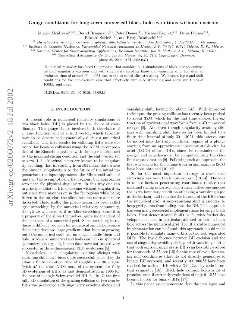
In Fig. 4 we compare data from this run with a run foridentical parameters except that instead of Eq. (44) weuse Eq. (43) with η = 2.8/M for the shift. The differencesare quite small in the case of this Schwarzschild run.

In Fig. 5 we show the maximum of the shift and theroot-mean-square value of the Hamiltonian constraint asa function of time. After a short time interval of lessthan 100M (recall that previous runs with vanishingshift lasted only to about 30-40M !), evolution is approx-imately frozen for more than 3000M . The observed driftin various quantities is crucially affected by the value of ηthat determines the diffusion in the hyperbolic Gamma-driver. In Fig. 5 we compare again the two versions ofthe Gamma-driver, and note that two different values ofη, 2.0/M and 2.8/M , are used to obtain long term stabil-ity. It is a matter of experimentation to find a suitablevalue of η in dependence on the various parameters inthe run. Runs may crash before 100M for a bad choiceof η. On the other hand, once determined for a particu-lar initial data set and set of grid parameters, we foundthat the runs were rather robust under small variations.It would be useful to have a dynamic determination andadaptation of η, but this is currently not available.

Having established the basic features and the stabil-ity of our gauge choice, we want to study convergencefor Schwarzschild. A crucial issue is whether we ob-tain convergence near the puncture. We choose threegrid sizes and resolutions: 201 points in both the x- andz-directions for a resolution of 0.025M , 401 points at0.0125M , and 801 points at 0.00625M . With a Courantfactor of 0.25 in the BSSN evolution scheme it takes 160,320, and 640 iterations, respectively, for an evolutiontime of 1M . The outer boundary is at about 5M . We

13

0 5 10x(M)

0

0.2

0.4

0.6

0.8

1

α

0 5 10−0.6

−0.4

−0.2

φ

0 5 100

0.1

0.2βx

0 5 10−4e−05

0

4e−05

8e−05

K

FIG. 4. Schwarzschild black hole evolved for t = 1000M .Shown is a comparison along the x-axis between two versionsof the hyperbolic Gamma-driver for the shift, Eq. (43) (dashedline) and Eq. (44) (solid line).

0 1000 2000 30000.00

0.05

0.10

0.15

0.20

0.25

max

(βx )

0 1000 2000 3000 t (M)

0.000

0.005

0.010

0.015

0.020

0.025

rms(

H)

FIG. 5. Schwarzschild blackhole evolved for t = 3000M . Shown are the maximum ofthe shift and the root-mean-square value of the Hamiltonianconstraint as a function of time, again for two versions of thehyperbolic Gamma-driver for the shift, Eq. (43) (dashed line)and Eq. (44) (solid line), with diffusion parameter η = 2.0/Mand η = 2.8/M , respectively. After a short time interval dur-ing which lapse and shift adjust themselves dynamically, theevolution slows down significantly.

0 1 2x (M)

0

1e−4

2e−4

rms(H

)

(dx = 0.025M) / 16(dx = 0.0125M) / 4(dx = 0.00625M) / 1

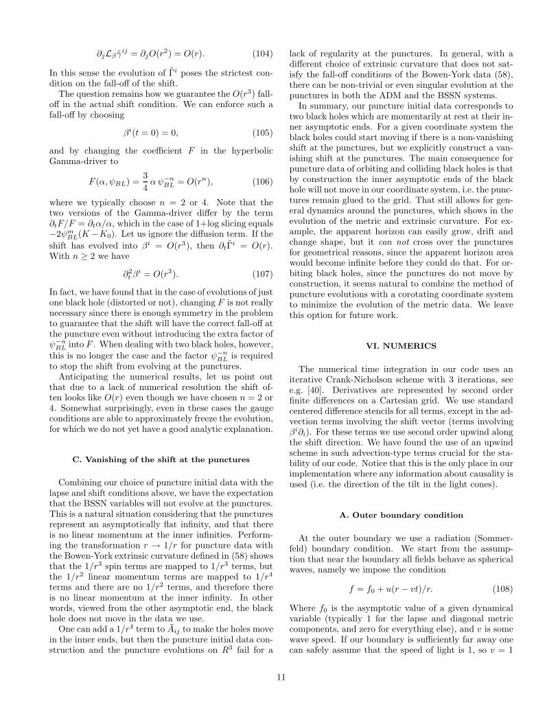
FIG. 6. Schwarzschild black hole evolved to t = 5M atthree high resolutions, demonstrating second order conver-gence at the puncture.

choose the same gauge as in (115), except that in F weuse ψ−4

BL instead of ψ−2BL for a broader profile of the shift

near the puncture.Fig. 6 shows the Hamiltonian constraint along the x-

axis near the single Schwarzschild puncture at the threeresolutions, rescaled by the corresponding factors ex-pected for second order convergence. The coincidence ofthe three lines indicates clean second order convergence.Therefore, for such high resolutions the BSSN systemexhibits the expected regular and convergent behaviournear the punctures. It is remarkable that even at a fourtimes coarser resolution of 0.1M the evolutions remainstable.

Note in particular that the shift in Fig. 2 seems tobe linear at the puncture, in contrast with the expectedO(r3) behaviour. Fig. 7 shows the effect of different pow-ers of ψBL in the shift equation for the grid parameters ofthe medium resolution run of the convergence test. Weuse the shift equation (44), and

F =3

4αψ−n

BL, η = 2.0/M, (116)

with different values for n. Fig. 7 shows the shift fort = 1M . Note the resolution that is required to makethe O(r3) behaviour visible for n ≥ 2. By t = 10M ,the shift for n = 2 is no longer completely resolved atthe puncture with a grid spacing of 0.0125M , but as wehave seen, even at coarser resolutions the approximateO(r) behaviour of the shift at the puncture allows stableevolutions.

B. Evolution of a single, distorted black hole

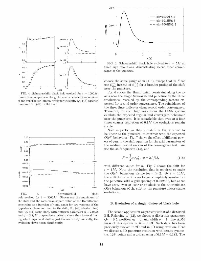
The second application we present is that of a distortedBH. Referring to [42], we choose a distortion parameterQ0 = 0.5, position η0 = 0, and width σ = 1. The ADMmass of this system is M = 1.83. Such data has beenpreviously evolved in 2D and in 3D using excision. Herewe discuss a 3D puncture evolution with octant symme-try, 1293 points and a grid spacing of 0.1M = 0.183. The

14

0 1 2

x (M)

−0.02

0.00

0.02

0.04

0.06

0.08

0.10

0.12

βx

n=0n=1n=2n=3n=4

FIG. 7. Schwarzschild black hole evolved for t = 1M .Shown is the effect of varying the power n in ψ−n

BLin the

shift equation for βx along the x-axis.

outer boundary is at about 12.8M . For the gauge we use1+log slicing with the initial lapse not unity but givenby (95) and the hyperbolic shift condition (44) with

f = 2α−1ψ4BL, F =

3

4αψ−2

BL, η = 1.25/M ≈ 0.68. (117)

In Fig. 8, we show the evolution of the lapse and theshift component βx along the x-axis. Note that the shift,although vanishing initially, develops the needed profilesimply through its evolution equation, without any spe-cial initial condition. After a short while, the evolutioneffectively freezes, allowing the waves to propagate on aneffectively fixed BH background, just as one would like.

For comparison, we show in Fig. 9 the evolution ofthe radial component of the metric, γrr/ψ

4BL, for the

new gauge condition (lower panel) and for a singularityavoiding slicing run with 1+log slicing and vanishing shift(upper panel). For 1+log slicing and vanishing shift wesee the well-known slice stretching effect. With the newgauge evolution is slowed significantly at late times. Thepeak of the metric near x = 0.5M grows to about 12 bytime t = 20M and does not grow significantly after thatuntil t = 400M (lower panel), while for vanishing shiftalready at t = 30M the peak in the metric has reached40 without any sign of slowing growth (upper panel).

For the new gauge we expect that we can reliably ex-tract the waveform for the ring-down, and this is indeedthe case as shown in Fig. 10.

C. Head-on collision of two Brill-Lindquist punctures

The third application we present is that of a headon collision of two Brill-Lindquist BH’s. The param-eters for these simulations are m1 = m2 = 0.5M ,C1 = {0, 1.1515M, 0}, C2 = {0,−1.1515M, 0}, wherem1 and m2 are the masses of the BH’s and C1 and C2

are the locations of the two punctures. These parame-ters correspond to an initial separation of the BH’s equal

0 2 4 6 8 10 12 14x(M)

−0.05

0

0.05

0.1

0.15

0.2

βx

0 2 4 6 8 10 12 140

0.2

0.4

0.6

0.8

1

α

t=0Mt=5Mt=10Mt=20Mt=30Mt=50Mt=100Mt=200Mt=400M

FIG. 8. Lapse and shift for the evolution of a single dis-torted BH. After around 20M , the evolution of lapse and shiftslows down significantly (note the time labels). The approachto the final profile in lapse and shift is not monotonic.

to that of an approximate ISCO configuration as deter-mined in [43]. Such data has been previously evolvedwithout shift with the Lazarus technique that combinesshort, fully numerical evolutions with a close limit ap-proximation for the wave extraction [9] (see [12] for runsstarting at larger separation).

We present two types of runs for the head-on collisionstarting at the approximate ISCO separation. In the firsttype we use 1+log slicing and the hyperbolic Gamma-driver (43) with

f = 2α−1, F =3

4αψ−4

BL, η = 2.8/M. (118)

with an initial lapse equal to one and an initial shift equalto zero. We also use the transition fish-eye with param-eters a = 3, s = 1.2M and r0 = 5.5M . This places theouter boundary at a distance of 25.8M with central res-olutions 0.128M , 0.064M and 0.032M and gridsizes 963,1923 and 3843 respectively in octant mode.

In Fig. 11 we show the extracted ℓ = 2 and m = 0waveforms until t = 80M for all three resolutions. Thecode actually continued beyond t = 140M at the highestresolution (more than t = 200M at the lower resolutions)before we stopped it, due to the fact that it was computa-tionally fairly expensive. Initially there seem to be somesmall amplitude oscillations superposed on the larger os-cillations. These seem to be related to an initial wavepulse in the lapse moving outwards as the lapse collapsesfrom its initial value, which is not quite handled by thewave extraction procedure. However these oscillationsdecrease with increasing resolution. With f = 2α−1ψ4

BL

15

0 2 4 6 8 10 12 14x(M)

0

2

4

6

8

10

12γ rr/ψ

4 BL

t=0Mt=10Mt=20Mt=30Mt=50Mt=100Mt=200Mt=400M

0 2 4 6 8 10 12 140

10

20

30

40

t=0Mt=10Mt=20Mt=30M

FIG. 9. The evolution of the radial metric functionγrr/ψ

4BL for a distorted BH along the x−axis. The upper

panel shows the slice stretching in the metric for singularityavoiding slicing with vanishing shift, while the lower panelshows the metric for the new gauge conditions. Without shiftthe metric grows out of control after t = 40M , while withthe new shift condition a peak begins to form initially butlater almost freezes as lapse and shift drive the BH into anessentially static configuration (note the time labels).

as we used in the previous examples instead of (118), theoscillations are larger, probably because the lapse is moredynamic in the initial phase of the evolution. But as al-ready mentioned in Sec. V A, even with f = 2α−1ψ0

BL thelapse collapses at the punctures. After about t = 80Mwe see some non-quasi-normal features in the waveform,that are most probably due to contaminations from theouter boundary.

For a wave signal A extracted at three resolutions, ∆,2∆ and 4∆ the order of convergence, σ, can be estimatedas

σ = log2

∣

∣

∣

∣

A(4∆) −A(2∆)

A(2∆) −A(∆)

∣

∣

∣

∣

. (119)

In Fig. 12 we show this estimate of the convergence fac-tor for the three waveforms from Fig. 11. Several featuresin this figure deserve comment. First of all, for the first15M the signal is very small, so the estimate of the con-vergence order is not very accurate. Secondly, the phaseevolution of the waveforms is somewhat resolution depen-dent. This means that the curves cross over each other atdifferent times, leading to the spikes clearly visible in theplot. The differences in phase evolution seem to decreasewith increasing resolution, although only at somewherebetween first and second order. However excluding theinitial part and the spikes, we see a reasonable secondorder convergence in the waveforms up to t = 80M .

0 20 40 60 80t (M)

−0.6

−0.3

0

0.3

0.6

ψ20

even

(M

)

3D(1313x0.183)

fit

0 30 60 90 120 150 180−0.6

−0.3

0

0.3

0.6

2D(300x29)3D(131

3x0.183)

3D(1313x0.183)

FIG. 10. The solid line shows the ℓ = 2,m = 0 waveformextracted at a radius of 5.45M for the even-parity distortedBH described in the text, while the two dashed lines showthe result of the same simulation carried out in the 2D and3D code with vanishing shift. The 2D code crashes at aroundt = 100M and the 3D code crashes around t = 40M . Thelower panel shows a fit for the time interval from t = 9Mto t = 80M to the two lowest quasi normal modes of theBH for the new gauge conditions in 3D, confirming that thering-down of the distorted BH is simulated accurately.

In Table I, we try to circumvent the problem of thedifferently evolving phase by locating the extrema of thewaveforms and estimating the convergence order usingthese extremal values even if they do not occur at thesame time. As can be seen, except for the first maximum,there is generally nice second order convergence in theamplitude. In the case of the first maximum, it can beseen from Fig. 11 that the difference between the threeresolutions is very small and that especially the lowestresolution is influenced by the pulse in the lapse movingout.

As a second type of gauge choice we use maximal slic-ing and the hyperbolic gamma driver condition with the

Extremum log2 |(A(4∆) − A(2∆))/(A(2∆) − A(∆))|

1 1.172 2.113 2.004 1.955 1.966 2.24

TABLE I. The convergence of the amplitude for the firstsix local extrema of the extracted ℓ = 2, m = 0 waveforms forthe head on collision of two Brill-Lindquist BH’s extracted atradius 18.5M .

16

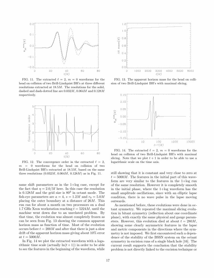
FIG. 11. The extracted ℓ = 2, m = 0 waveforms for thehead on collision of two Brill-Lindquist BH’s at three differentresolutions extracted at 18.5M . The resolutions for the solid,dashed and dash-dotted line are 0.032M , 0.064M and 0.128Mrespectively.

FIG. 12. The convergence order in the extracted ℓ = 2,m = 0 waveforms for the head on collision of twoBrill-Lindquist BH’s extracted at 18.5M , based on the samethree resolutions (0.032M , 0.064M , 0.128M) as in Fig. 11.

same shift parameters as in the 1+log case, except forthe fact that η = 2.0/M here. In this case the resolutionis 0.128M and the grid size is 803 in octant mode. Thefish-eye parameters are a = 4, s = 1.2M and r0 = 5.0Mplacing the outer boundary at a distance of 26M . Thisrun ran for about a month on two processors on a dual1.7 GHz Xeon workstation reaching t = 5224M , until themachine went down due to an unrelated problem. Bythat time, the evolution was almost completely frozen ascan be seen from Fig. 13 showing the common apparenthorizon mass as function of time. Most of the evolutionoccurs before t = 200M and after that there is just a slowdrift of the apparent horizon mass giving about 10% errorat t = 5000M .

In Fig. 14 we plot the extracted waveform with a loga-rithmic time scale (actually ln(t+ 1)) in order to be ableto see the features in the beginning of the waveform, while

FIG. 13. The apparent horizon mass for the head on colli-sion of two Brill-Lindquist BH’s with maximal slicing.

FIG. 14. The extracted ℓ = 2, m = 0 waveforms for thehead on collision of two Brill-Lindquist BH’s with maximalslicing. Note that we plot t + 1 in order to be able to use alogarithmic scale on the time axis.

still showing that it is constant and very close to zero att = 5000M . The features in the initial part of this wave-form are very similar to the features in the 1+log runof the same resolution. However it is completely smoothin the initial phase, where the 1+log waveform has thesmall amplitude oscillations, since with an elliptic lapsecondition, there is no wave pulse in the lapse movingoutwards.

As mentioned before, these evolutions were done in oc-tant symmetry. We repeated the maximal slicing evolu-tion in bitant symmetry (reflection about one coordinateplane), with exactly the same physical and gauge param-eters. However, this evolution died at about t = 280M ,showing some clearly asymmetric features in the lapseand metric components in the directions where the sym-metry is not imposed. We first encountered such a depen-dence of the stability of the BSSN system on the octantsymmetry in excision runs of a single black hole [16]. Thecurrent result supports the conclusion that the stabilityproblem is not directly linked to the excision technique or

17

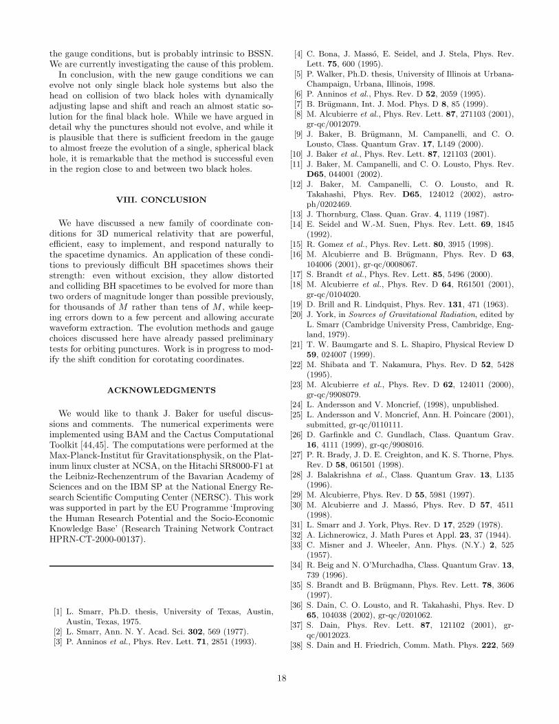
the gauge conditions, but is probably intrinsic to BSSN.We are currently investigating the cause of this problem.

In conclusion, with the new gauge conditions we canevolve not only single black hole systems but also thehead on collision of two black holes with dynamicallyadjusting lapse and shift and reach an almost static so-lution for the final black hole. While we have argued indetail why the punctures should not evolve, and while itis plausible that there is sufficient freedom in the gaugeto almost freeze the evolution of a single, spherical blackhole, it is remarkable that the method is successful evenin the region close to and between two black holes.

VIII. CONCLUSION

We have discussed a new family of coordinate con-ditions for 3D numerical relativity that are powerful,efficient, easy to implement, and respond naturally tothe spacetime dynamics. An application of these condi-tions to previously difficult BH spacetimes shows theirstrength: even without excision, they allow distortedand colliding BH spacetimes to be evolved for more thantwo orders of magnitude longer than possible previously,for thousands of M rather than tens of M , while keep-ing errors down to a few percent and allowing accuratewaveform extraction. The evolution methods and gaugechoices discussed here have already passed preliminarytests for orbiting punctures. Work is in progress to mod-ify the shift condition for corotating coordinates.

ACKNOWLEDGMENTS

We would like to thank J. Baker for useful discus-sions and comments. The numerical experiments wereimplemented using BAM and the Cactus ComputationalToolkit [44,45]. The computations were performed at theMax-Planck-Institut fur Gravitationsphysik, on the Plat-inum linux cluster at NCSA, on the Hitachi SR8000-F1 atthe Leibniz-Rechenzentrum of the Bavarian Academy ofSciences and on the IBM SP at the National Energy Re-search Scientific Computing Center (NERSC). This workwas supported in part by the EU Programme ‘Improvingthe Human Research Potential and the Socio-EconomicKnowledge Base’ (Research Training Network ContractHPRN-CT-2000-00137).

[1] L. Smarr, Ph.D. thesis, University of Texas, Austin,Austin, Texas, 1975.

[2] L. Smarr, Ann. N. Y. Acad. Sci. 302, 569 (1977).[3] P. Anninos et al., Phys. Rev. Lett. 71, 2851 (1993).

[4] C. Bona, J. Masso, E. Seidel, and J. Stela, Phys. Rev.Lett. 75, 600 (1995).

[5] P. Walker, Ph.D. thesis, University of Illinois at Urbana-Champaign, Urbana, Illinois, 1998.

[6] P. Anninos et al., Phys. Rev. D 52, 2059 (1995).[7] B. Brugmann, Int. J. Mod. Phys. D 8, 85 (1999).[8] M. Alcubierre et al., Phys. Rev. Lett. 87, 271103 (2001),

gr-qc/0012079.[9] J. Baker, B. Brugmann, M. Campanelli, and C. O.

Lousto, Class. Quantum Grav. 17, L149 (2000).[10] J. Baker et al., Phys. Rev. Lett. 87, 121103 (2001).[11] J. Baker, M. Campanelli, and C. O. Lousto, Phys. Rev.

D65, 044001 (2002).[12] J. Baker, M. Campanelli, C. O. Lousto, and R.

Takahashi, Phys. Rev. D65, 124012 (2002), astro-ph/0202469.

[13] J. Thornburg, Class. Quan. Grav. 4, 1119 (1987).[14] E. Seidel and W.-M. Suen, Phys. Rev. Lett. 69, 1845

(1992).[15] R. Gomez et al., Phys. Rev. Lett. 80, 3915 (1998).[16] M. Alcubierre and B. Brugmann, Phys. Rev. D 63,

104006 (2001), gr-qc/0008067.[17] S. Brandt et al., Phys. Rev. Lett. 85, 5496 (2000).[18] M. Alcubierre et al., Phys. Rev. D 64, R61501 (2001),

gr-qc/0104020.[19] D. Brill and R. Lindquist, Phys. Rev. 131, 471 (1963).[20] J. York, in Sources of Gravitational Radiation, edited by

L. Smarr (Cambridge University Press, Cambridge, Eng-land, 1979).

[21] T. W. Baumgarte and S. L. Shapiro, Physical Review D59, 024007 (1999).

[22] M. Shibata and T. Nakamura, Phys. Rev. D 52, 5428(1995).

[23] M. Alcubierre et al., Phys. Rev. D 62, 124011 (2000),gr-qc/9908079.

[24] L. Andersson and V. Moncrief, (1998), unpublished.[25] L. Andersson and V. Moncrief, Ann. H. Poincare (2001),

submitted, gr-qc/0110111.[26] D. Garfinkle and C. Gundlach, Class. Quantum Grav.

16, 4111 (1999), gr-qc/9908016.[27] P. R. Brady, J. D. E. Creighton, and K. S. Thorne, Phys.

Rev. D 58, 061501 (1998).[28] J. Balakrishna et al., Class. Quantum Grav. 13, L135

(1996).[29] M. Alcubierre, Phys. Rev. D 55, 5981 (1997).[30] M. Alcubierre and J. Masso, Phys. Rev. D 57, 4511

(1998).[31] L. Smarr and J. York, Phys. Rev. D 17, 2529 (1978).[32] A. Lichnerowicz, J. Math Pures et Appl. 23, 37 (1944).[33] C. Misner and J. Wheeler, Ann. Phys. (N.Y.) 2, 525

(1957).[34] R. Beig and N. O’Murchadha, Class. Quantum Grav. 13,

739 (1996).[35] S. Brandt and B. Brugmann, Phys. Rev. Lett. 78, 3606

(1997).[36] S. Dain, C. O. Lousto, and R. Takahashi, Phys. Rev. D

65, 104038 (2002), gr-qc/0201062.[37] S. Dain, Phys. Rev. Lett. 87, 121102 (2001), gr-

qc/0012023.[38] S. Dain and H. Friedrich, Comm. Math. Phys. 222, 569

18

(2001), gr-qc/0102047.[39] S. Dain, Phys. Rev. D (to be published) (2001), gr-

qc/0103030.[40] M. Alcubierre et al., Phys. Rev. D 62, 044034 (2000),

gr-qc/0003071.[41] M. Alcubierre et al., Int. J. Mod. Phys. D 10, 273 (2001),

gr-qc/9908012.[42] S. Brandt, K. Camarda, and E. Seidel, in Proceedings of

the 8th Marcel Grossmann Meeting on General Relativity,edited by T. Piran (World Scientific, Singapore, 1999),pp. 741–743.

[43] T. W. Baumgarte, Phys. Rev. D 62, 024018 (2000).[44] B. Brugmann, Ann. Phys. (Leipzig) 9, 227 (2000), gr-

qc/9912009.[45] Cactus, http://www.cactuscode.org.

19