Climate and ice sheet evolutions from the last glacial ... - CP
COMMUNICATIONS ON PURE AND APPLIED MATHEMATICS, VOL. xxv, 337-367 (1972)
Non-Commuting Random Evolutions, and an Operator-Valued Feynman-Kac Formula*
R. HERSH University of New Mexico
AND G. PAPANICOLAOU
Department of Mathematics, University Heights and Courant Institute, N. Y. U.
Introduction A “random evolution” in general is a solution of an evolution equation with
random coefficients. That is, it is a mathematical model for a dynamical system subject to stochastic controls.
The present paper treats equations of the form
where y and f are elements in a Banach space L, x ( t ) is a Markov process, and, for each x , V(x) is the generator of a semigroup of operators on L. These equations have recently come into increasing use as models for such physical phenomena as wave propagation in random media. In such situations, one seeks a “law of averages” which, hopefully, predicts the expected outcome, without requiring detailed knowledge of the short-time fluctuations of the medium.
Formal procedures for finding this expected outcome have recently been developed by several authors, e.g., Kubo, Stratonovich, M. Lax, Keller and Papanicolaou and others, in a wide variety of physical contexts. Formal results have of course run ahead of rigorous convergence proofs. One of our principal motivations has been to provide a rigorous formulation for the asymptotic representation obtained formally by the two-time perturbation method in Papanicolaou-Keller [lo].
0, to e “ f , where P is a certain non-symmetric quadratic form in V(x) . We assume that the average value of Y(x) is zero, that, for each x, V(x) generates a contraction semi- group, and that x ( t ) is ergodic with finitely many states. Our methods would extend to a more general state space if we assume that there exists at least one
We prove that the expected value of y ( t / 9 ) converges, as E
* The paper was written while the first author was a Visiting Member of the Courant Institute and was supported by NSF GP 27719; the work of the second author was supported by NSF Grant GP-27209. Reproduction in whole or in part is permitted for any purpose of the United States Government.
337 Q .1972 by John Wiley & Sons, Inc.
338 R. HERSH AND G. PAPANICOLAOU
state whose recurrence time has finite mean and variance. (In another paper [9] we give an asymptotic theorem for the case when x ( t ) is a general renewal process, with values independent of renewal times.) Section 1 concludes with an application to transport theory; we obtain the diffusion approximation for trans- port in an inhmogcneous medium as the mean free path goes to zero.
The case when the operators V(x) all commute with each other has been treated by R. Hersh and M. Pinsky [4], using different methods. They allow the random evolutions to grow exponentially. Here we restrict ourselves to contrac- tions, but we are able to dispense completely with any commutativity condition. On the other hand, we assume that p generates a semigroup, whereas in the commutative case this is part of the conclusion. If x ( t ) is reversible (invariant under a reversal of time-direction), P is symmetric and reduces to the same expression as that found by Hersh and Pinsky in the commutative case.
In Section 2, x ( t ) is any Markov process, not necessarily ergodic, and with arbitrary state space. Assuming only that the random evolution y ( t ) exists and has a finite expected value u ( t ) (as elements in some Banach space L) we show that u ( t ) is itself the solution of a differential equation, a deterministic equation of the form
d dt - u(t, x ) = Q u + V(%)U )
where Q is the infinitesimal generator of the Markov process x ( t ) . This theorem is an operator-valued version of the classical Feynman-Kac
formula. The version given by Kac provided a stochastic representation for the solution of
where Q is the generator of a Markov process with state-space X, and u, f and g are real-valued. We show that this formula is valid, when suitably reinterpreted, if the values of u ( t , x ) and f ( x ) are elements of a Banach space L, and g(x) V ( x ) is, for each x, an operator from L into itself. This was proved by R. J. Griego and R. Hersh [3] in the special case of a finite state-space, but they did not notice the connection between their result and the Feynman-Kac formula. As a concrete application, we recover Kac’s solution of the telegraph equation
1 2a
U t t + - Ut = u,, ,
obtained originally by a different argument. We also show how to construct partial differential equations of arbitrarily high order which are solved by sto- chastic integrals.
NON-COMMUTING RANDOM EVOLUTIONS 339
We conclude the paper by applying our operator Feynman-Kac formula to the asymptotic theorem of Section 1. We obtain in this way a new singular perturbation theorem for a deterministic Cauchy problem. Entirely aside from its probabilistic interpretation, this result can be regarded as a theorem in the functional calculus of non-commuting unbounded operators. As an example of this application, we give a new asymptotic theorem for first order hyperbolic systems with variable coefficients. In the limit, we get a single, second-order parabolic equation with variable coefficients. For constant coefficients this result was first proved by Pinsky [l 13.
Such systems arise in transport theory if the velocities of the moving particles depend on position. They also were introduced by Frisch [I41 in his study of random wave propagation. This paper was written while the first-named author was a visiting member
of the Courant Institute. He would like to take this occasion to thank the many friends there who made his stay enjoyable and fruitful. The interest and en- couragement of Mark Kac also calls for our hearty thanks. Finally, we gratefully acknowledge the advice of Prof. S. Varadhan, whose insight and knowledge have been an invaluable help to us.
1. An Asymptotic Theorem for Non-Commuting Random Evolutions
Let L be a Banach space with elements f. For each a = 1,2,. . . , n, V, denotes the generator of a strongly continuous semigroup of contraction operators T,(t), f 2 0, on L. 9 = n (domain of Vs Vj V,) is assumed to be dense in L.
We assume also that all real linear combinations of the V, are closed. This is true for concrete cases of differential operators we consider here and it will permit us to apply freely the interchange of limiting operations and action by such operators.
Let Q = (qu) be an n-by-n matrix which generates an ergodic continuous-
time Markov chain; that is, 0 qij < m for i # j , 2 qu = 0 and Q has zero
as a simple eigenvalue. The Markov chain generated by Q will be denoted by x ( t * ) and its state space by (1, . . . , n} so that Vz($.) is a random operator-valued function of t* which takes on finitely many values. For ergodic Q it is known that if we normalize the components pi of the unique left null vector of Q by
the condition 2 pi = 1, then limp,, P { x ( t * ) = j } = fig, independent of the
initial state x ( 0 ) . Moreover, the limit is approached at an exponential rate. If p , > 0, the state i is called ergodic. In this case, the path x ( t * ) returns to i infinitely often with probability one. We assume without loss of generality that p1 > 0 so that (1) is an ergodic state.
We shall denote by Ei integration with respect to the probability measure on the sample paths starting from state i. When we write E without subscripts, we
8.j .k
n
f=1
n
6-1

340 R. HERSH AND G. PAPANICOLAOU
mean integration with respect to the probability measure on the paths whose starting point is distributed with the invariant measure { p i } .
We let a, be the epoch of the k-th return to state (1); a, E 0. The successive return times 7, = a,,, - a, are independent random variables, and for k 2 1 are identically distributed. We let N ( t ) = min {k I a, 2 t } ; aN(t) , the epoch of the first visit to (1) a t or after time t , is a stopping time for x ( t ) . The time T,, = aI of the first entry into state (1) depends on the initial state, and hence it will be denoted by $) ; 7:') = T, = a, . An elementary estimate shows that the random variables {T,, k 2 1) have a density function n ( u ) which satisfies
(1.1) I I (u ) c e-"
for some positive constants c, a. (This estimate is a simple generalization of a similar result for discrete-time finite-state chains, cf. Feller [2], p. 345, Problem 8.) The random variable # satisfies a similar estimate. We denote the mean of T,, k 2 1, by p and their variance by 2. We assume without loss of generality that t/e2p is an integer, and we let 5 = a(t/es,,)+l . Any a,, and in particular 6, is a stopping time for x ( t ) .
We now define a "random evolution" M(')(s, t ) as the unique solution of the stochastic initial value problem
dM(') 1 dt E - = - M(')vE(#,c*) ,
M y $ , s) = I . t > s ,
Here I denotes the identity operator. Equation (1.2) is obtained by substitu- ting t = t* in the equation dM'"/dt* = EM(') V E ( p ) . I t is in the time scale of (1.2) that we obtain a nontrivial limiting result for the expected value of M(')(s, t ) when s and t are fixedand E - 0 .
From (1.2) it follows that
In view of this property we can write an explicit representation of M(')(s, t ) in terms of the semigroups T,(t), which can at the same time serve as a definition of M(')(s, t ) independent of (1.2). Let t:, tt, . . . , t: denote the successive jump times of x ( t * ) in the time interval ($lea, t / e a ] . The random integer Y = V(S /E%, t/$) counts the number of jumps in the relevant interval. I t is easy to see now that
(1.4) MI')($, t ) = TE(r,8a)(&' - s/&)T,(t:)(~t: - ~ t : ) * . T,( , : ) (~/E - ~ t : )
is the required representation. If at the jump points the derivative in (1.2) is taken as the one-sided right derivative, then it follows from (1.4) that M(')(s, t )

NON-COMMUTING RANDOM EVOLUTIONS 34 1
is right continuous at the jump times. It is clear from (1.4) how to interpret M"'(a,, a,) when a, and a, are stopping (or Markov) times for x ( t * ) . When E = 1 and s = 0, then (1.4) reduces to the random evolution M ( t ) introduced in [3]. From (1.4) and our assumption that T , ( t ) is a contraction, it is clear that M(')(s, t ) is a contraction, for any value of s, t, E .
An elementary computation, using either (1.4) or (1.2) and (1.3), shows that M(')(s, t ) is the solution operator for the backward equation @/dr = - (114 Vzcelr:)Y), 0 5 4 Y EL. That is, ~ ( s ) = u(')(J, t )y ( t ) . Technicalities caused by the non-commutativity of M and V make the backward solution operator more convenient for us. However, by the change of variable t' = t - s our theorem is immediately applicable to d " ( t - t', t), the solution operator for the forward problem dy/dt' = (l/e) VE( t , / ca )~ , t' 2 0.
Our goal is to compute the limit, as E + 0, of E,{M"'(O, t ) f } when t > 0 is fixed. Our main theorem says that under natural hypotheses this limit exists, is independent of i, and is a semigroup of contractions, which we shall call etVJ To define the generator P of the limiting semigroup, we introduce
In Lemma 2 we show that P' is well-defined for f €9. For applications, a more explicit representation of P is desirable. Before
giving the proof of our theorem, we make a short excursion to derive some formulas for P.
None of the material from this point up to the statement of Theorem 1 is used subsequently, except in the application to transport theory at the end of this section. The reader may if he desires Proceed directly to Theorem 1.
First we note that from ( 1 -5) it is clear that
where 0 =( p tributing x(0) according to the invariant measure, P(x(0) = i} = p i , we have
r =( T. Since the probability in (1.7) is conditioned on dis-
P { x ( p ) = a, x ( r ) = 8) = P { x ( p ) = a} prob {x ( r ) = p I x ( p ) = a}
= PaPap ( r - P ) 9
where p i , ( t ) = etO is the standard notation for the transition probabilities of the
342 R. HERSH AND G. PAPANICOLAOU
n Markov chain x ( t ) . Since x p i Vi = 0, we can replace japap(r - p) under the
summation sign by ka(pap(r - p) - 1
If we make the change of variable u = r - p, v = Y + p, (1.7) becomes
Now, because flap(u) - f ir converges to zero at an exponential rate as u -+ 00,
both integrals on the right of (1.8) converge as T-+ 00.
Since the second is multiplied by 1/T, it vanishes in the limit, and we are left with
P = 2 v a vp f a r ( pap(u> - du *
This is symmetric if and only if pa pap pa fib. , which is the known condition (see, e.g., Feller [2], Chapter 15, (11.3)) that the process x ( t ) is reversible. In fact, from (1.5) it is clear that VT and P are symmetric forms if the distribution of x ( t ) is invariant under time-reversal.
(Pap(u) - pa) du is the value
of the Laplace transform of paa(u) - pp at the origin. Since the matrix paB(u) is annihilated by d/du - Q and equals the identity a t u = 0, its Laplace trans- form, as a function of 1, is (1 - Q);;, and we have
We can simplify P further by noticing that !OW
P = 2 pa Va Vp lim 1-0 1
Given any matrix M, let cofaBp (M) denote the cofactor of the a,@-th elementof M. Then, using Cramer’s rule and 1’Hospital’s rule,
To check this formula, and also as a method of computing the normalized left null vector (pa), it is helpful to notice that

NON-COMMUTING RANDOM EVOLUTIONS 343
where
d dA. 2-0 y-1
K = (-l)"-'- det (A - Q) 1 = Scof,,, (Q) .
To see this, recall that Q*, the "adjoint" matrix whose transpose is the matrix cofa,p ( Q ) , satisfies
Q*Q = QQ* = det Q . I = 0 ,
so that the rows of Q* are left null vectors and the columns of Q* are right null vectors for Q. But since zero is a simple eigenvalue of Q, they must in fact be multiples, respectively, of p l , . . . , p , and (1, . . . , 1). Therefore, cofaep ( Q ) is independent of B, and, since Z p , = 1,
Notice that (- l)"-l K is the product of the non-zero eigenvalues of Q. These are negative, or, if complex, come in conjugate pain, so K > 0.
The numerator, (@A) cofP,,(1 - Q)IA=o, is the coefficient of the linear term 1 in the polynomial cofP,, (A - Q ) , and is therefore equal to Zy2a,p 4py,T, (- where 4pPr,ya denotes the determinant of the matrix obtained by deletingthe B-th and y-th rows and the y-th and a-th columns from Q.
A simpler expression can be given if P is symmetric by using a result from the commutative case. For, if the Va are mutually commutative, P can be sym- metrized in the usual procedure of elementary linear algebra, replacing the coefficients of Va Vp and Vp Va by the average of the two coefficients. The resulting form, the symmetric part of P (symm P), could also be obtained by symmetrizing ( 1.5),
where y , ( T ) denotes the occupation time in state a for x ( t * ) , 0 t* Again using zfla V, = 0, together with E ( y , ( T ) ) = Tp, , we get
T.
344 R. HERSH AND G . PAPANICOLAOU
Now, in [4] it is shown that this symmetric form is equal to
(In case n = 2 , Although all diagonal terms are absent from this representation, it is in fact
easy to diagonalize it, using the condition z p a V, = 0 to find the cross terms V, Vs as linear combinations of the squares Vg .
f 1 by definition.)
For example, if n = 3, we use
2Pa PB V a Vp = p'y VZ, - P: V : - V s to obtain
3
symm V = ~ Z V : pi 2 B. i=l f . k # i P k
f # k
We conclude this discussion of v by considering the case when qij is inde- pendent of j for j # i. (This means that once x ( t * ) decides to jump out of its present state, it is equally likely to go to any other state.) We shall obtain a strikingly simple and suggestive formula for p as a sum of squares.
It will simplify our formulas to introduce the notation ai = (1 - n ) / q i , . Then we have
1 - n 1 4rj = -
ai 4
In this case, x ( t * ) is reversible, so that v = symm p.
if i # j , qii = -.
Next let A(r, A) be an r-by-r matrix with elements equal to A on the main diagonal and 1 elsewhere. Notice that det Q = (a,. . . det A(n, 1 - n). Now all rows of A(r, 1) are identical, so A = I is an (r - I)-fold zero of det A(r, A). Also, the columns of A(r, 1 - r) sum to zero; hence, A = 1 - 7 is also a zero of det A(r, A). Therefore, det A(r, A) = ( A - l).-l(A + r - 1). Also, pi = a,(al + *
cofy,y (Q) = ay(al * * un)-l det A(n - 1, 1 - n) * + an)-1, so that z p i V, = 0 = 2 a, Vj . Therefore,
= qy(al - .an)-y-n)n-9(-1) and
= a, ap(a, - * * un)-l det A(n - 2, 1 - n) = a, ap(al * * * u p ( -n)"-l( -2) .
Consequently,
NON-COMMUTING RANDOM EVOLUTIONS 345
But squaring 2: ai Vi = 0, we get
so that
( I t is tempting to let n -+ m formally, and interpret the result in terms of an infinite state space.) With this example we conclude our discussion of v.
We are now ready to state and prove Theorem 1. All limits are understood to be strong limits.
THEOREM 1. If v generates a strongly continuous semigroup on L, 9 and (/? - v ) 9, /? > 0, are dense in L, Q is ergodic, and
then lim Ei{M(e’(O, t > > = e“ . r -0
Proof: The key idea is to introduce an operator S, , defined by
s, = E,{M“’(O, E2 TI)} . S, is the expected value of a random evolution corresponding to an orbit of x ( t * ) from one entry into the ergodic state (1) to the next re-entry into {I} . Keeping t / E * p integer-valued, we prove in Lemmas 1, 2 and 3 that
(1.9) s, = z + E2pv + 0 ( E S ) ,
so that (S,)l’as’’ -+ elv . Then we conclude the proof by showing that
Ei{M‘*’(O, t ) } - (S,)l”*’
goes to zero strongly. Intuitively, this is easy to understand. When E is small, the path x(tSI.9) will, with high probability, pass through state (1) very soon after the initial time 0, and again very shortly before the final time t . The factors S, represent the expected evolution from one entry into {I} until the next entry. The successive evolutions are independent and identi- cally distributed, and the expected number of recurrences is t / E * p; therefore,
346 R. HERSH AND 0. PAPANICOLAOU
it is reasonable to conjecture that E,{M(e)(O, t)} - d = u(t /a~p)+l . Then, by the triangle inequality,
For the proof, we set
II (Ei{MYO, t ) } - n f l l s I1 ( S F - c ' v I I + 11 (E,{M'"(O, &'.a)} - s y y 11
+ I IEi{M(8)(Oy t ) - ~'~'(0, E'oN(t/ea))}fII
+ llEi{M(e'(oy e2 3) - M("(Oy -!? uN(t/$))}fll
These four terms are estimated in Lemmas 4, 6, 7 and 8.
iterating (1.2). We abbreviate Ve(rJ to V ( r ) , and get, for f E 9, Our first step is to obtain integral equations for M(')(s, t ) by integrating and
(1.10)
(1.11)
(1.12)
& M ( 8 ) ( ~ , t ) = I + 1 V(rl.2) dr
& 8
MU(s, t ) = I + & r / 'V(r/e2) dr + e2 l l V ( r , / E ' ) V ( r / e 2 ) dr, dr
+ A Jtlr/rlM(')(s, ro) V(r,/e2) V(rl/e2) V(r/e*) dr, dr, dr . & 8 8 8
To prove (1.9), we set o = 0, t = ~ 8 7 ~ in (1.12) and apply El to both sides. We let S, , i = 1, 2, 3, denote the resulting integrals, so that
LEMMA 1. For any f E 9, S, f = 0.
Proof This could be proved by elementary methods, but we use an argu- ment that we shall need again, in Lemmas 2 and 8. Its use here serves as an intro- duction to ideas to follow. Our main tool is Wald's theorem (see Doob, Stochartic P~ocesscs, p. 350): "If the zi are independent and identically distributed, and
NON-COMMUTING RANDOM EVOLUTIONS 347
V
v is a finite stopping time for the sequence of the zi , then E { Z zj} = E{v}E{z}." '
1 Note first that
for any j 2 1, in view of the time-homogeneity of x ( t * ) . Next, observe that for any T we have
I-1
J u N - 1 JUN-I
For each j the integrals
random variables, whose mean (for any distribution of x ( 0 ) ) is given by
V(r)fdr are independent and identically distributed
Moreover, a simple renewal argument shows that E ( N ( T ) ) = T / p + o(T) . Therefore, by Wald's theorem,
Since
348 R. HERSH AND G. PAPANICOLAOU
are bounded independent of T, we can combine terms to get
On the other hand,
which is zero by hypothesis. Therefore,
Letting T + 00, we get S, f = 0, as was to be proved.
LEMMA 2 . For any f E 9, pf is well deJined and equals S, fle2p.
Proof The proof uses a random partition of the triangle {p , I 10 6 p r T), similar to the partition of the (0, T) interval in Lemma 1. However, a more delicate argument is needed, using the optional stopping theorem for martingales along with the Wald theorem used in Lemma 1.
We start out by noticing that
S, f = - 1 E l ( ] " r ~ V ( p / e z ) V(r/e2) dr dp)f e2 0
for j 2 1, by the time-homogeneity of x ( t * ) , and the strong Markov property.
NON-COMMUTING RANDOM EVOLUTIONS
P
349
r
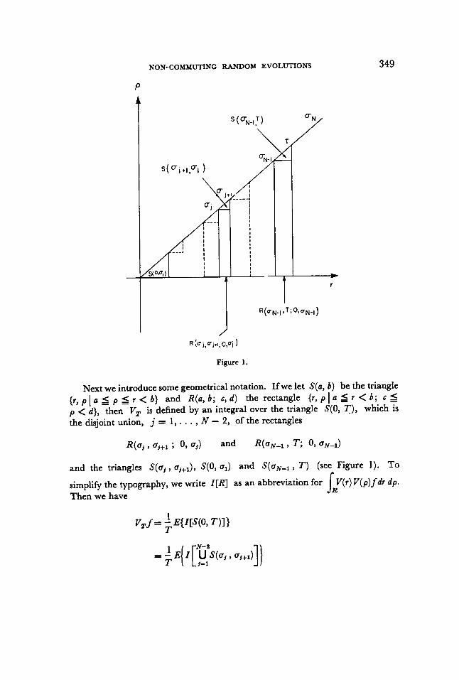
Next we introduce some geometrical notation. If we let S(a, 6 ) be the triangle {r , p I a 5 p r < 6 ) and R(a, 6 ; t, d) the rectangle {r, p I a 2 r < 6 ; t 5 p < d } , then V, is defined by an integral over the triangle S(0, T) , which is the disjoint union, j = 1, . . . , N - 2, of the rectangles
R(aj, aj+1 ; 0, aj) and R ( ~ N - , , T; 0, aN-1)
and the triangles S ( u j , aj+J, S(0, a,) and S(aN-, , T) (see Figure 1). To
simplify the typography, we write Z[R] as an abbreviation for Then we have
R. HERSH AND C. PAPANICOLAOU 350
(1.13)
To prove the lemma we must look at these five terms one after another. We start out by using an argument identical to that of Lemma 1 to show that, as T + my the first term goes to S p f / e a p .
We have
Because x ( t ) is a Markov process and .(aj) = (11, the summands are in- dependent and identically distributed, and have expected value equal to Sa flea.
Again, as in Lemma 1 , we have E ( N ) = T/p + o ( T ) ; of course, the same formula holds for E(N - 2) and so, using Wald's theorem, the first term of (1.13) is
Saf I 0) eap T
To show that the second term is 0 (1 / T ) , we write
s E ( 4 ) SUP II v u VJll Y
a.b
which is finite because f €9 and the recurrence times of the finite-state chain x ( t ) have moments of all orders.
The third term is 0(1 /T) by a similar argument; we find
Next we consider the last term of (1.13). We have, using the Markov property of x(r) and the fact that x(aN-J = (1) to conclude that the two integrals
NON-COMMUTING RANDOM EVOLUTIONS
are independent,
35 1
The first term on the right of this inequality is clearly O( l /T) . We claim that the second term is zero, identically in T. To prove this, we observe that the integrals
V(p) dp constitute a sequence of independent random variables, each of
which has mean zero, by Lemma 1. The claim then follows by Wald's theorem. s.:"'
It remains to estimate the fourth term in (1.13), which is
For any j, we have
using the Markov property, the definition of uj and applying Lemma 1 to the second factor. Again by the Markov property, the expected value of the second factor is not changed if we condition on the values of
352 R. HERSH AND G. PAPANICOLAOU
for k < j . Since the second factor is still zero, the conditional expectation of the j-th double integral
is zero, given the value of the k-th double integral for all k < j. That is, the sequence of partial sums of these double integrals is a martingale, and so, using again the optional stopping theorem with N( T) as our stopping time and sub- tracting the last two terms which have mean zero by Lemma 1, we find that
Returning to (1.13), we now have
Letting T + m, we obtain Vf = &flEP p 9
as claimed.
LEMMA 3. For all f €9, Ss f = o(e8 ) .
Proof: In the triple integral which defines S, , make a change of variables similar to those performed in Lemmas 1 and 2. Since M(')(a, 6) is a contraction for any a, 6, E, we get
which is finite by (1.1) and the definition of 9, and proves the lemma.
LEMMA 4.
Proof Since V is by assumption the generator of a strongly continuous semigroup elp, it suffices, by Theorem 3.6 and Remark 3.7, p. 51 1, of Kato [8 ] , to show that
lim, (S,)""' = etF.
1 lim- (S, - I) f = pf a-0 Eap
NON-COMMUTING RANDOM EVOLUTIONS 353
for f in a dense subset of the domain of 9 such that ( p - 9)9, B > 0, is also dense. Now, since 9 is by assumption dense in L and is a subset of n (domain of ViVr) which is a subset of the domain of p, the result follows from
substituting from Lemmas 1, 2, '3 into the expansion f.f
s, = I + s, + s, + &.
In view of Lemma 4, the proof of the theorem will be complete if we show that
(1.14) II(E,{M'"'(O, t ) } - sye*fl)) f 11 --+ 0
In preparation, we give a factorization lemma.
LEMMA 5. Let p1 and pz be stopping times for x ( t * ) and a a stopping time such that p1 a pa and .(a) = (1). Then
Ei{M(E'(&2 p1, E2 p2)> = Ei{M'e'(&2 p1, E2 a)}E,(M"'(O, e2 p2 - E2 a ) }
Proof Let denote the 0-algebra of events generated by x ( t * ) for s t* t . In view of the strong Markov property and the time homogeneity of the chain as well as property (1.3), we have
Ei{M'e'(&2 p1 , &a p,)} = E,{M'"(&2 p1 , E2 .)M'"(&2 a, &I p, ) }
= E,{E,{M'e'(&2p1, &2a)M("(&2a, E S P 2 ) 1 AS}}
= E,{M'e'(&2p1, &2a)Ei{M'~)(&%, E2 p2) I At}} = E,{M'e'(&Z p1, E' a)}E,{M"'(O, e2 p2 - e2 a ) } .
This completes the proof of the lemma. Recall the notation d = t~( t ,~a , , )+~ .
LEMMA 6. For f E 9,
Proof: Repeatedly using Lemma 5 , with stopping times 0; = 7:' + T~ + * - - + T ~ - , we have
354 R. HERSH AND 0. PAPANICOLAOU
(using the time-homogeneity of x ( t * ) in the last step). Therefore,
l l ( E i { M y 0 , E2 5 ) ) - S:'e") f 11 = l l (Ei {My0, & * T f ) ) ) - Z)sy'pf 11 (1.15) 5 11 ( E ~ { M ( ~ ) ( o , e2 7:)) - Z) ( s ~ / ~ ' c - e">fll
+ I ~ ( E ~ { M ( ~ ) ( O , e*Tf))) - z>e*'fll . The first of these two terms is a t most 2II(S;le*" - etP) f 11, which vanishes as E 4 0 by Lemma 4. T o estimate the second term, we use ( l . l O ) , setting etV f = g. Since P commutes with erv and the domain of P is contained in the domain of V, , g = ctv f is in the domain of Va for f E 9. We therefore have
The lemma is proved. Now recall that N ( t ) = min {k I a, )= f}.
LEMMA 7. For f E 9,
Proof By ( l . l O ) ,
6 EE(QN(tla') - +*) SUP II v, f I1 s 4% - UN-1) SUP II v, f I1 = EP SUP II v, f I1 .
a
(I
a
In view of Lemmas 6 and 7, (1.14) will be established and the theorem will be proved once we establish
LEMMA 8. For f €9,
NON-COMMUTING RANDOM EVOLUTIONS 355
Let Nl = min (N( t / ea ) , flea p) , NB = max ( N ( t / t z ) , t /e2 p ) .
‘Then, using (1.1 l) , we get, after the usual change of variables,
IIEi(M‘”(0, aN(t/a’)) - ~‘”(0, ep 8))fII
(1.16)
The first term on the right is zero, since
Each of the two sums in the last equation is clearly a martingale, since the terms are independent and, according to Lemma 1, have mean zero. Therefore, by Doob’s optional stopping theorem, each sum has mean zero, and so has the difference of the two.
I t remains to estimate the double integral in (1.16). To do this, we return to the notation and methods of Lemma 2. The region of integration is now the union of the triangle S(oN1 , uNa) and the rectangle R(aN1 , aN, ; 0, uNl). We parti- tion this region into the disjoint union, Nl sj s N, - 1, of the triangles S(aj , c,+~) and the rectangles R(a, , oj+l , 0, uj).l First we consider the integral over the union of the rectangles R(a, , ; 0, a,). This integral differs by a single term from the difference between two random sums, one up to Nl and one up to N,. If we can show that each term in the sum has conditional expectation zero, given the values of the preceding terms, then we can conclude as in Lemma 2 that the integral is zero, by the optional stopping theorem for mar- tingales. A typical term in this random sum is
= r M f 8 ’ ( 0 , ea p)V(p) dpIu’+’ V ( r ) dr f.
Of the two factors on the right, the first depends on the path . r ( t * ) only for
l See Figure 2.

356 R. HERSH AND G. PAPANICOLAOU
P
Figure 2.
t* 5 0, , whereas the second is independent of the path before the stopping time a, , by the Markov property. Hence they are independent, and we have
which is zero because
by Lemma 1, independently of i and j . I t is clear from our discussion that this result is not changed by conditioning on
[“”’ [ukM(s)(O, E* p) V ( p ) dp V ( r ) dr f J E ~ JO
for k < j. I t follows that the partial sums form a martingale, the sum up to either Nl or N, terms has mean zero, and the difference between the two sums, which is the integral over the region below the “staircase” in Figure 2, has mean zero.
NON-COMMUTING RANDOM EVOLUTIONS 357
Thus (1.16) has been reduced to
(1.17)
by Wald’s theorem, since - u, = 7, are independent and identically distributed for j 2 1.
A standard result in renewal theory tells us that N(t /c2) is asymptotically normal, with mean t/eZ ,u and variance ,us. Schwarz’ inequality then giVeS
E2 E{IN(t/&2) - t /&2 ,u1} &2(E{(N(t/E2) - t / E 2 , u ) 2 } ) ” 2
for E sufficiently small. The proof of both the lemma and the theorem is com- plete.
Next we give a corollary that will. be used in Section 2, where we convert our limit theorem for a stochastic equation into a singular perturbation theorem for a deterministic equation.
COROLLARY. Let f a , a = 1, . . . , n, be a given n-tuple in the Bmach space L.
Then
Proof: Since 9 is dense in L, and M‘”(0, t ) and etv are contractions, it Abbreviating is sufficient to prove the corollary for f a E 9, a = 1 , , . . , n.
358 R. HERSH AND G. PAPANICOLAOU
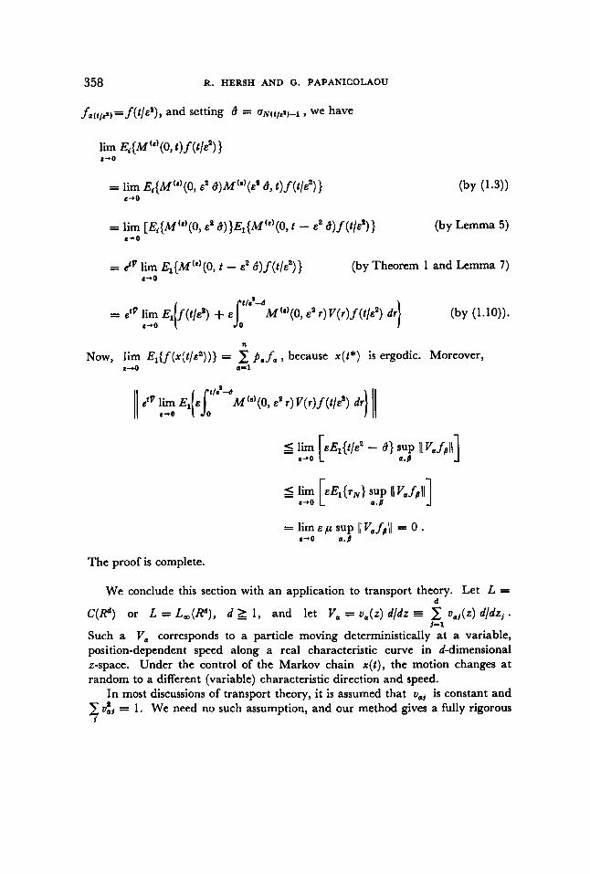
fi(t,rs)= f(t /&'), and setting 6 = q,7(:la¶)-1 , we have
= lim [E,{M"'(o, E' ~ ) } E , { M ' ~ ' ( O , t - E' & ) f ( t / E ' ) } (by Lemma 5 ) 8-0
= etv lim E,(M'"(O, t - E' B ) f ( t / e * ) } (by Theorem 1 and Lemma 7) S+O
e' r) V(r) f ( t /e ' ) dr
n
Now, lim E l { f ( x ( t / e 2 ) ) } = 2 p a f a , because x ( t * ) is ergodic. Moreover, S 4 a-1
r 1
- 1 S+O a . P
r 1
The proof is complete.
We conclude this section with an application to transport theory. Let L =
C ( P ) or L = L,(Rd), d 2 1, and let Va = v a ( z ) d/dz E 2 uaj(z) d/dz,.
Such a Va corresponds to a particle moving deterministically at a variable, position-dependent speed along a real characteristic curve in d-dimensional z-space. Under the control of the Markov chain x ( t ) , the motion changes at random to a different (variable) characteristic direction and speed.
In most discussions of transport theory, it is assumed that va, is constant and 2 u:j = 1. We need no such assumption, and our method gives a fully rigorous
d
j=l
j

NON-COMMUTING RANDOM EVOLUTIONS 359
derivation of the diffusion approximation. On the other hand, we do'have the undesirable restriction that the index a runs over a finite index set. Also, additional discussion would be needed to take account of sources and boundaries.
Under reasonable conditions, each V, generates a group of contractions. If d = 1, it suffices that
def
exists for all z E R1 and has an inverse function hi1( z) for all z E R1. This will be true, for example, if each v, has constant sign and is bounded, locally integrable, and satisfies Iu,(z)I 2 6 > 0 for some constant 6. Then one finds that V, gen- erates the group
The space L of data and solutions can be taken as L,(R1) or as C(R1). Given any generator Q, we can now construct the random evolution,
M(')(s, t ) , as a random product of operators Ta(e7), given by formula (1.4). Given an initial distribution of positions f a ( z ) , our theorem tells us that if the
resultant direction 2 p,, u,(z) is identically equal to the zero vector in Rd, and
if the deterministic motion along each characteristic curve is speeded up by a sufficiently large factor 1 / ~ while the random change of direction is speeded up by l/$, then the distribution of positions at time t is close to the solution of h / d t = Pu, u(0) = Zp,f , ( z ) . We need only check that #' generates a semi- group. Now, v is clearly a differential operator of second order. Moreover the principal part of P (terms of order exactly 2) depends only on symm P. (We refer to the discussion of P and symm P given earlier in this section before the statement of Theorem 1.)
Because the commutators VaV, - V,V, are of order less than 2, one sees
n
a-1
that the principal part of P is just (1/2k) 2 qEa,,,ua(z)vb(z) d$/dz, dz, . From R& Ll -. ,
the fact, shown above, that symm P is the limit of a covariance matrix, it is clear that qEa,,,, the coefficients of s y m m P, constitute a non-negative form. It follows that v,(z)vp(z)qaa,,, is also non-negative, so that P is a second- order elliptic or degenerate-elliptic differential operator. Then known theorems on parabolic equations tell us that P does generate a contraction sexnilgroup, and Theorem 1 applies. We return to this example at the end of Section 2, where we show its connection with a hyperbolic system of partial differential equations, which degenerates to a single parabolic equation.
360 R. HERSH AND G. PAPANICOLAOU
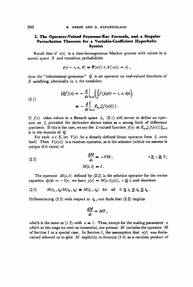
2. The Operator-Valued Fe\ynman-Kac Formala, and a Singular Perturbation Theorem for a Variable-Coefficient Hyperbolic
System
Recall that if x ( t ) is a time-homogeneous Markov process with values in a metric space X and transition probabilities
p ( t - s, x, A ) = P ( x ( t ) E A I x ( s ) = x ) ,
then the “infinitesimal generator” Q is an operator on real-valued functions of X satisfying, identically in t , the condition
If f ( x ) takes values in a Banach space L, (2.1) still serves to define an oper- ator on f, provided the derivative shown exists as a strong limit of difference quotients. If this is the case, we say the L-valued function f ( x ) = Ez,a{f(x(t))}l,=g is in the domain of Q.
For each x E X, let V(x) be a densely defined linear operator from L onto itself. Then V(x(s) ) is a random operator, as is the solution (which we assume is unique if it exists) of
dM - = - V M , ds
M(t, c) = I .
t > , s z o ,
The operator M(s, t ) defined by (2.2) is the solution operator for the vector equation &/& = -Vy; we have y ( s ) = M(s, t )y( t ) , s t, and therefore
(2.3) M(t , , t,)M(t, , ts ) = M(t, , ts ) for all 0 t, 5 t, ts
Differentiating (2.3) with respect to t, , one finds that (2.2) implies
- M V , dM -- dt
which is the same as (1.2) with E = 1. Thus, except for the scaling parameter E
which at this stage we omit as inessential, our present M includes the operator M of Section 1 as a special case. In Section 1, the assumption that x ( t ) was finite- valued allowed us to give M explicitly in formula (1.4) as a random product of
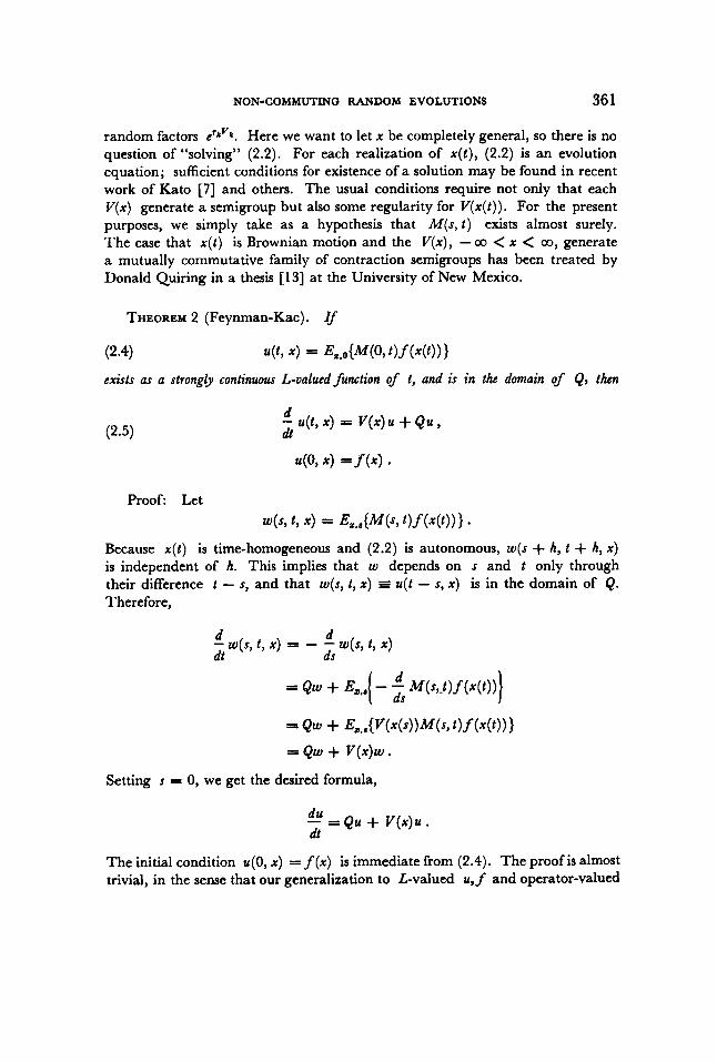
NON-COMMUTING RANDOM EVOLUTIONS 36 1
random factors e‘kvk. Here we want to let x be completely general, so there is no question of “solving” (2.2). For each realization of x ( t ) , (2.2) is an evolution equation; sufficient conditions for existence of a solution may be found in recent work of Kato [7] and others. The usual conditions require not only that each V(x) generate a semigroup but also some regularity for V(x( t ) ) . For the present purposes, we simply take as a hypothesis that M(s, t ) exists almost surely. The case that x ( t ) is Brownian motion and the V ( x ) , - 00 < x < 00, generate a mutually commutative family of contraction semigroups has been treated by Donald Quiring in a thesis [13] at the University of New Mexico.
THEOREM 2 (Feynman-Kac). r f
(2.4) 44 4 = Ez,o{M(O, t ) f ( x ( t > ) 1 exists as a strongly continuous L-valued function of t, and is in the domain of Q, then
Proof Let t , 4 = Ez.,{M(4 t ) f ( x ( t ) ) 1 -
Because x ( t ) is time-homogeneous and (2.2) is autonomous, w(s + h, t + h, x ) is independent of h. This implies that w depends on s and t only through their difference t - s, and that w(s, t , x ) = u(t - s, x ) is in the domain of Q. Therefore,
d d dt ds - w(s, t , x ) = - - w(0, t , x )
Setting s = 0, we get the desired formula,
du - = QU + V(X)U . dt
The initial condition u(0, x ) = f ( x ) is immediate from (2.4). The proof is almost trivial, in the sense that our generalization to L-valued u, f and operator-valued

362 R. HERSH AND 0. PAPANICOLAOU
M, V hardly alters the argument. The only difference is that VM # MV, and so we have to be careful to throw the differentiation from the t-variable onto the 9- variable. The main analytic difficulties are buried in our hypothesis. In concrete examples, it may not be easy to determine for which f it is true that u( t , x ) is in the domain of Q. Nevertheless, as our examples will show, the theorem dots give a striking unification to some hitherto disconnected formulas and provides a method to generate new formulas at will.
.
EXAMPLE 1. Let x ( t ) be Brownian motion, X = R1, L = R1, and V(x) a real-valued, continuous function, bounded from above. Then (2.2) is solved explicitly by
and (2.4) becomes
where E. is the Wiener integral over paths that start from the point x . Q is now i#/dxsJ and our theorem says that (2.6) solves the partial differential equation
This, of course, is the classical Feynman-Kac result.
EXAMPLE 2. Let X be the integers from 1 to nJ x ( t ) any n-state continuous- time Markov chain, and each V(x) the generator of a strongly continuous semigroup of operators on L. Then we are in the setting of Section 1 of the present paper, but without requiring x ( f ) to be ergodic or c ~ ” ‘ ~ ) to be a con- traction. Each f ( x ) is an n-tuple of elements of L, and Q is a matrix (qrr), r , ~ = 1 , . . , , n. I t is shown in Griego-Hersh [3] that in this case u(tJ x ) = Ez,o{M(O, t ) f ( x ( t ) ) } is finite and strongly continuous for all n-tuples f ( x ) . Of course u is in the domain of Q, since Q is bounded. If we write the finite-valued independent variable x in the customary manner as a subscript, i = 1, . . . , n, we have uJt) = E,{M(O, t ) f ( x ( t ) ) } as a solution for the system of operator differential equations
. .
This result was given in [3]. If the Vd are elliptic differential operators, (2.7) is
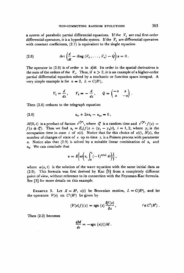
NON-COMMUTING RANDOM EVOLUTIONS 363
a system of parabolic partial differential equations. If the Vi are real first-order differential operators, it is a hyperbolic system. If the Vi are differential operators with constant coefficients, (2.7) is equivalent to the single equation
d dt
det (- - diag (Vl,. . . , V,) - Q) u = 0 . (2.8)
The operator in (2.8) is of order n in dldt. Its order in the spatial derivatives is the sum of the orders of the V i . Thus, if n > 2, it is an example of a higher-order partial differential equation solved by a stochastic or function space integral. A very simple example is for n = 2, L = C(R1),
d d dz dz , V a = - - , Q=(,' ( I a ) . v, = -
Then (2.8) reduces to the telegraph equation
(2.9) U t t + 2au, - u,, = 0 ,
M(0, t ) is a product of factors c~:"~, where t: is a random time and e':v*f(z) = f ( z f t r ) . Thus we find ui = E i { f ( z + (y , - y8)t} , i = 1,2, where yi is the occupation time in state i of x ( t ) . Notice that for this choice of x ( t ) , N(s) , the number of changes of state of x up to time s, is a Poisson process with parameter a. Notice also that (2.9) is solved by a suitable linear combination of ul and u2. We can conclude that
u = E(w( x, l( - ds)) ,
where w(x, t ) is the solution of the wave equation with the same initial data as (2.9). This formula was first derived by Kac (61 from a completely different point of view, without reference to its connection with the Feynman-Kac formula. See [3] for more details on this example.
EXAMPLE 3. Let X = R1, x ( t ) be Brownian motion, L = C(R1), and let the operators V ( x ) on C1(R1) be given by
Then (2.2) becomes
dM ds - = - - ~ g n ( x ( t ) ) M .

364 R. HERSH AND C. PAPANICOLAOU
The solution operator is again strongly continuous and a contraction, and is given by
(2.10)
For this example we take 59 = C1(R2) and we see that here (2.5) takes on the form
(2.11)
40, *, 4 = f ( x , 4 - From both (2.10) and (2.11) it follows that x = 0 is a highly singular point. Let us therefore assume that x > 0 and define u+ and u- by
u+(t, x , 2) = u(ty x, z) y
u-(t, x, 2) = u(t , - x , 2 ) ,
w(ty x, 2) = u+(t, x , z) + u-(t, x, 2) . It is now easy to verifir that, for x > 0, w satisfies the partial differential equation
aw 1 a a f 1 aaf at az az 2 ax= 2 a x 2 - (0, x, z) = af ( x , z) - af (-x, z) + -- ( x , z) + -- (-x, 2) ,
EXAMPLE^. Let us again consider the same spaces and process as in Example 3 with B = Ca(R1) and V(x) defined by
NON-COMMUTING RANDOM EVOLUTIONS 365
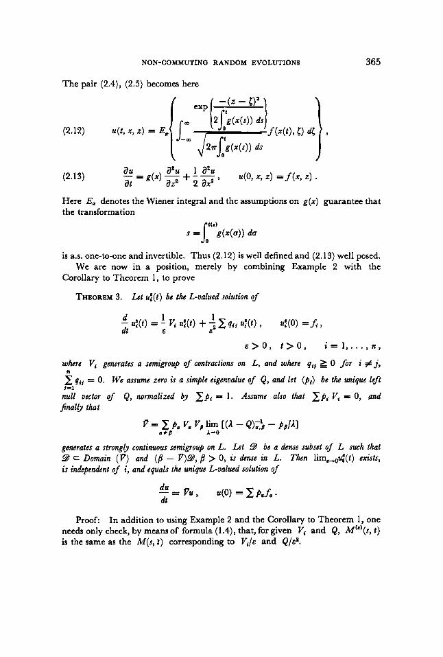
The pair (2.4), (2.5) becomes here
aU a s u 1 atu
at ata 2 ax2 ’ (2.13) - = g ( x ) - +-- 4 0 , x, 4 = A X , 4 ’
Here En denotes the Wiener integral and the assumptions on g ( x ) guarantee that the transformation
s =L(”g(”(u)) d o
is ass. one-to-one and invertible. Thus (2.12) is well defined and (2.13) well posed. We are now in a position, merely by combining Example 2 with the
Corollary to Theorem 1, to prove
THEOREM 3. Lef u f ( t ) be the L-valued solution of
d 1 1 dt E & - d ( t ) = - Vf U X t ) + 7 2 qrj u:(t> I u;(o) =fi J
E > O , t > O , i = l , . . . , n ,
where Vi gemrates a semigroup of contractions on L, and where qir 2 0 for i # j ,
2 qij = 0. W e assume zero is a simple eigenvalue o f Q, and Let ( p i ) be the unique hjit
null vector o f Q, normalized b~ 2fit = 1. Assume also that Z p , Vi = 0, and
n
9-1
finally that
P = 2 Pa Va Vp lim [ ( A - Q)i,\ - Pj/Al a # P 2-0
generates a strongly continuous semigroup on L. Let 9 be a dense subset of L such that .9 c Domain (P) and (/I - V)B, /I > 0, is dense in L. Then lim-G(t) exists, is indcpendent of i, and equals the unique L-valued solution of
d u - = Pu , u(0) = c p a f , . dt
Proof In addition to using Example 2 and the Corollary to Theorem 1, one needs only check, by means of formula (1.4), that, for given Vf and Q, M(’)(s, t ) is the same as the M(s, t ) corresponding to Vile and Q/e*.

366 R. HERSH AND 0. PAPANICOLAOU
In operator notation, we have proved that
converges, as an operator on L", to etv II, where ll is a mapping of L" onto
L given by II(f& . . . , f,,) = 2 p,f, . This is a remarkable result from the view
point of the perturbation theory of linear operators, since it concerns a singular perturbation of non-commuting, non-selfadjoint, unbounded operators. Is there a way of understanding it apart from its stochastic interpretation?
An example of Theorem 3 of particular interest is the application to transport theory given at the end of Section 1 , where V, = v, (2 ) dldz. For v, independent of z, and initial values f independent of a, this is a singular perturbation theorem first proved by Pinsky [l 11, using the direct method of Fourier trans- formation and expanding the solution in powers of E . This method had the merit of providing an error estimate, which we have not attempted to give. On the other hand, it is not clear how pure analytic methods could achieve the extension to variable v, obtained here by the combination of probabilistic and operator- theoretic arguments. In this case, u8 is the solution of a first-order hyperbolic system of partial differential equations with variable coefficients. p, as we saw at the end of Section 1 , is a second-order elliptic or degenerate-elliptic differential operator with variable coefficients, and us 4 u the solution of a single second- order parabolic equation with space-dependent coefficients.
n
1=1
Bibliography [l] Doob, J. L., Stachastic Proccsses, New York, John Wiley and Sons, 1953. [2] Feller, W., An Introduction to Probability Theory, Vol. I, John Wiley and Sons, 1966. [3] Griego, R., and Hersh, R., Theory of random evolutions with applications to partial d i f f imt ia l
[4] Henh, R. and Pinsky, M., Ran&m evolutions are asumptoticalb Gaussian, Comm. Pure Appl.
[5] Kac, M., On the distribution of certain Wimerfunctionals, Trans. Amer. SOC., Vol. 65, 1949, pp.
[6] Kac, M., Some stochastic problems in physics and mathematics, Magnolia Petroleum Co., Lectures
[7] Kato, T., Linear evolution equatiom of "hyperbolic" t f ie , J. of Faculty of Science, Univ. of Tokyo,
[8] Kato, T., Perturbation Thcwy of Linear Opcratws, Springer, Berlin, 1966. [9] Papanicolaou, G. C., and Hersh, R., Sonu limit theorems for stochastic equations and applications,
to appear in Indiana U. Math. J. [lo] Papanicolaou, G., and Keller, J. B., Stochastic dt&rcntial equations with applications lo random
harmonic oscillatws and wave fw@agation in random media, SIAM Journal on Appl. Math., 20,
equations, Trans. Amer. Math. Soc., Vol. 156, 1971, pp. 405-418.
Math., Vol. 25, 1972, pp. 3344.
1-1 3,
in Pure and Applied Science, No. 2, 1956.
Vol. XVII, 1970.
1971, pp. 287-305.
NON-COMMUTING RANDOM EVOLUTIONS 367
[ 1 I] Pinsky, M., Dt&ential equatwns with a small parameter and the central limit theorem fw functwns & ? d on a Jnite Markov chain, Z . Wahrscheinlichkeitstheorie Verw. Gebiete, 9, 1968, pp. 101-1 11.
[I21 Pinsky, M., Multiplicatwe operator functionals of a Markov process, Bull. of the AMS, Vol. 77, 1971, pp. 377-380.
[13] Quiring, D., Random evolutions on di&wn processes, Z . Wahrscheinlichkeitsthcorie Verw.
[ 141 Frisch, U., Wave Pqbagation in Random Media, Probabilistic Methods in Applied Mathematics,
[I51 Stratonovich, R. L., Topics in the Thcory of Random Noise, Vol. I, 11, Gordon and Breach,
[I61 Lax, M., Classical noise, IV; Lung& methods, Review of Mod. Phys., Vol. 38, 1966, pp.
[17] Kubo, R., Stochashc Lwuvillc equation, Journal of Math. Phys., Vol. 4, 1963, pp. 174-183.
Received July, 197 1.
Gebiete, to appear.
cd. A. T. Bharucha-Reid, New York, Academic Press, 1968.
N.Y., 1963.
561-566.
Copyright © 2022 FDOKUMEN