Does Richard Feynman Dream of Electric Sheep? Topicson Quantum Field Theory, Quantum Computing, and

Computer Science

Thesis byJunyu Liu

In Partial Fulfillment of the Requirements for theDegree of

Doctor of Philosophy

CALIFORNIA INSTITUTE OF TECHNOLOGYPasadena, California

2021Defended May, 3, 2021

ii

© 2021

Junyu LiuORCID: 0000-0003-1669-8039

All rights reserved except where otherwise noted

iii

ACKNOWLEDGEMENTS

Caltech is really an amazing school with an excellent academic environment. Iam very lucky to have been here to receive so many educational opportunities,collaborations, and friendships. As a starting point of my professional career, I amtrying to be a theoretical physicist, a dream I have had from childhood. It has alsoprovided me an excellent platform to interact with great minds not only inside thecampus, but also the whole high energy physics and quantum information sciencecommunity. These important five years are treasures in my whole life.

Firstly, I wish to thank my advisors. I am lucky enough to be advised by three greatscientists at the same time, Clifford Cheung, John Preskill, and David Simmons-Duffin, (listed in the alphabetical order). They are great academic advisors, encour-aging me to solve important scientific problems, and giving me infinite suggestionsabout science and careers during my hard time.

Cliff is really a hero. I will remember infinite discussions we had on the fourthfloor of Downs-Lauritsen, or under the beautiful sunshine of Pasadena. For me,Cliff is a great mentor, teacher, and friend both in my academic and personal life.From him, I learned how to dive into problems deeply and think about importantproblems, and also be active on exploring different scientific problems and theirintersections. I believe those exceptional insights and profound knowledge willbenefit me throughout my life.

For me, John is one of the most outstanding wise men of our time, and it hasbeen my great honor to interact and work with him. When I was looking forresearch opportunities as a young graduate student, John brought a fascinatingworld, quantum information science, to me. What I have learned the most fromhim is to consider the long-term impact when choosing a research topic. As a greatmentor, John is very considerate and full of patience, of which I will have a lastingmemory.

David is a legend in theoretical physics. Working with David is a fantastic ex-perience. When I ask David questions, he can remember almost everything andwrite a crystal-clear explanation on the blackboard, including complicated series ofconformal block expansions. At the same time, David is also an excellent friend,and I am very thankful for his tolerance of my jokes, the outstanding organizationof the bootstrap collaboration, and the Caltech conformal group.

iv

To continue, I wish to thank other collaborators during my graduate school: NingBao, Alexander Buser, Shai Chester, Jordan Cotler, Hrant Gharibyan, MasanoriHanada, Masazumi Honda, Nicholas Hunter-Jones, Per Kraus, Walter Landry, AitorLewkowycz, Tianlin Li, Yue-Zhou Li, Don Marolf, David Meltzer, Ashley Milsted,Eric Perlmutter, David Poland, Grant Remmen, Vladimir Rosenhaus, Eva Silver-stein, Ning Su, Jinzhao Sun, Gonzolo Torroba, AlessandroVichi, GuifreVidal, YuanXin, Beni Yoshida, Xiao Yuan, Qi Zhao, Yehao Zhou, and You Zhou. Working withall of you has given me excellent and unforgettable memories!

I also wish to thank many other physics or STEM colleagues for your discussionsand friendships: Soner Albayrak, Victor Albert, Mustafa Amin, Guy-Gur Ari,Nima Arkani-Hamed, Yimu Bao, Yoni Bentov, David Berenstein, Dominic Berry,Fernando Brandao, Charles Cao, Marcela Carena, Sean Carroll, Xie Chen, GongCheng, Andrew Childs, Soonwon Choi, Clay Cordova, William Cottrell, ElizabethCrosson, Bartek Czech, Alex Dalzell, Maria Derda, Xi Dong, Rajeev Erramilli,Bradley Filippone, Liam Fitzpatrick, Weibo Fu, Andras Gilyen, Victor Gorbenko,Yingfei Gu, Charles Hadfield, Nicole Yunger Halpern, Connor Hann, Daniel Har-low, Jim Hartle, Tom Hartman, Patrick Hayden, Hong-Ye Hu, Yangrui Hu, RobertHuang, Alexander Jahn, Liang Jiang, Zhang Jiang, Denis Karateev, Kohtaro Kato,Emanuel Katz, Isaac Kim, Alexei Kitaev, Natalie Klco, Murat Kologlu, Shota Ko-matsu, Grisha Korchemsky, Petr Kravchuk, Richard Kueng, Henry Lamm, AdamLevine, Zhijin Li, Ying-Ying Li, Shu Lin, Ying-Hsuan Lin, Hong Liu, Jiahui Liu,Peter Love, Andreas Ludwig, Matilde Marcolli, Antonio Mezzacapo, Spiros Micha-lakis, AlexeyMilekhin, RyanMishmash, EvgenyMozgunov, Sepehr Nezami, HirosiOoguri, Sam Pallister, Julio Parra-Martinez, Fernando Pastawski, Geoffrey Pening-ton, Xiao-Liang Qi, Daniel Ranard, Sam Roberts, Junchen Rong, Slava Rychkov,Subir Sachdev, Burak Şahinoğlu, Prashant Saraswat, Martin Savage, Steve Shenker,Gary Shiu, Ashmeet Singh, Ronak Soni, Jon Sorce, Douglas Stanford, Leo Stein,Alexandre Streicher, Yuan Su, Jiarui Sun, Chong Sun, Brian Swingle, EugeneTang, Aron Wall, Tian Wang, Wanchun Wei, Mark Wilde, Mark Wise, Zhong-ZhiXianyu, Dan Xie, Hao-Lan Xu, Xi Yin, Yi-Zhuang You, Ellis Ye Yuan, PengfeiZhang, Shangnan Zhou, and Sisi Zhou.

Furthermore, I wish to thank so many wonderful places I’d had the chance tovisit: Stanford (thanks Xiao-Liang Qi and Eva Silverstein for hosting), UCSB/KITP(thanks Don Marolf for hosting), UCSD (thanks Yi-Zhuang You for hosting), UCBerkeley (thanks Soonwon Choi for hosting), Fermilab, University of Chicago,

v

University of Colorado Boulder, Princeton, IAS, Harvard, MIT, · · · , partially withthe help of the Simons collaborations on "It from Qubit" and "the NonperturbativeBootstrap", QOALAS collaboration, and the MURI collaboration on "QuantumCodes, Tensor Networks, and Quantum Spacetime." I also wish to thank the IASsummer school, TASI summer school, PsiQuantum Corporation for their study andinternship opportunities in Summer 2018, 2019, and 2020 respectively.

I wish to thank all my friends during my graduate school, especially Wen-LoongMa for his efficiency on eating, Honglie Ning for his driving skill, Burak Şahinoğluand Eugene Tang for some dark secrets about clubs, Weibo Fu, Masanori Hanada,Zhe Jia, Xiang Li, David Meltzer, Ashley Milsted and Yehao Zhou for their long-lasting friendship and help, Xinyue Dai, Nicole Jinglin Gao for her paintings, andRui Niu, Linrui Xiong for her arts. Moreover, I wish to thank all my IQIM friends,quantum information friends, Downs-Lauritsen fourth floor friends, high energyfriends, physics friends, and other friends during my graduate study. I also wishto thank my friends who interact with me in the Los Angeles local organizations,including Animals, Anime, Cats, Film, Hanfu, and Rave.

Thank you, Carol Silberstein, for your hard work in the Downs-Lauritsen fourthfloor; Mika Walton and Marcia Brown, for your hard work on my student fairs; andLaura Kim, Daniel Yoder, for your hard work about international students like me.Thank you Ryan Patterson for being my committee chair and making me suggestionsabout cyberpunk.

I wish to thank the University of Science and Technology of China, the HongKong University of Science and Technology, Nanjing University, Mcgill Universityand my undergraduate mentors, especially Robert Brandenberger, Yi-Fu Cai, GangChen, Henry Tye, and Yi Wang, who educated me as an undergraduate student andbrought me to the path of graduate study.

Finally, I wish to thank my cat Pafu for her lovely face. I wish to thank my father AnLiu my mother Li Ren and my grandmother Soqiong Zeng for their infinite amountof financial and emotional support.

vi

ABSTRACT

In this thesis, we mainly discuss three topics in theoretical physics: a proof ofthe weak gravity conjecture, a basic statement in the string theory landscape usingthe black hole entropy, solving the critical O(3) model using the conformal boot-strap method involving semidefinite programming, and numerical simulation of thefalse vacuum decay using tensor network methods. Those topics cover differentapproaches to deep understanding of quantum field theories using concepts andmethods of information theory, and computer science with classical and quantumcomputations.

vii

PUBLISHED CONTENT AND CONTRIBUTIONS

This thesis contains the following three scientific publications.

C. Cheung, J. Liu and G. N. Remmen, Proof of the Weak Gravity Conjecture fromBlack Hole Entropy, JHEP 10, 004 (2018), arXiv:1801.08546 [hep-th].J. Liu participated in the conception of the project and the writing of themanuscript, deriving a general formula between the extremal condition andWald entropy and applying the symbolic algebra on generalization to higherdimensions, and the writing of the manuscript.

S. M. Chester, W. Landry, J. Liu, D. Poland, D. Simmons-Duffin, N. Su andA. Vichi, BootstrappingHeisenbergMagnets and their Cubic Instability, arxiv:2011.14647 [hep-th].J. Liu participated in the conception of the project, thewriting of themanuscript,and the organization of the collaboration, applying and strengthening the islandand the OPE scan algorithm of the conformal O(3) model, applying the sym-bolic algebra to deriving crossing equations with symmetries, and searchingfor the critical gap with dynamical algorithms.

A. Milsted, J. Liu, J. Preskill and G. Vidal, Collisions of false-vacuum bubble wallsin a quantum spin chain, arXiv: 2012.07243 [quant-ph].J. Liu participated in the conception of the project, including numerical simula-tions on the dynamical evolution and entanglement/energy flux determinationof the kink scattering process using software, as well as the writing of themanuscript.

viii

TABLE OF CONTENTS

Acknowledgements . . . . . . . . . . . . . . . . . . . . . . . . . . . . . . . iiiAbstract . . . . . . . . . . . . . . . . . . . . . . . . . . . . . . . . . . . . . viPublished Content and Contributions . . . . . . . . . . . . . . . . . . . . . . viiTable of Contents . . . . . . . . . . . . . . . . . . . . . . . . . . . . . . . . viiiList of Illustrations . . . . . . . . . . . . . . . . . . . . . . . . . . . . . . . xiList of Tables . . . . . . . . . . . . . . . . . . . . . . . . . . . . . . . . . . xxiChapter I: Introduction: aspects of "cyberpunkian" quantum field theory . . . 1

1.1 Space opera and Cyberpunk . . . . . . . . . . . . . . . . . . . . . . 11.2 Quantum field theory . . . . . . . . . . . . . . . . . . . . . . . . . 51.3 Simulating quantum field theory using quantum devices . . . . . . . 91.4 Conformal field theory and large-scale optimization . . . . . . . . . 121.5 The theoretical landscape and data science . . . . . . . . . . . . . . 161.6 Some comments . . . . . . . . . . . . . . . . . . . . . . . . . . . . 20

Some physics . . . . . . . . . . . . . . . . . . . . . . . . . . . . . 20Black hole thought experiment and quantum information

science . . . . . . . . . . . . . . . . . . . . . . . 20It from qubit and the non-perturbative bootstrap . . . . . . . 21Church-Turing Thesis in 2021 . . . . . . . . . . . . . . . . 23

CS-inspired physics and physics-inspired CS . . . . . . . . . . . . . 24Theoretical considerations . . . . . . . . . . . . . . . . . . 24Benchmarking quantum devices using fundamental physics . 25High energy physics in the low energy lab . . . . . . . . . . 26

Towards the future . . . . . . . . . . . . . . . . . . . . . . . . . . . 27Waiting for quantum technology . . . . . . . . . . . . . . . 27Fundamental science using oracles . . . . . . . . . . . . . . 28Companies, colliders . . . . . . . . . . . . . . . . . . . . . 31

Chapter II: Proof of the Weak Gravity Conjecture from Black Hole Entropy . 332.1 Introduction . . . . . . . . . . . . . . . . . . . . . . . . . . . . . . 332.2 Proof of ∆S > 0 . . . . . . . . . . . . . . . . . . . . . . . . . . . . 38

Assumptions . . . . . . . . . . . . . . . . . . . . . . . . . . . . . . 38Positivity Argument . . . . . . . . . . . . . . . . . . . . . . . . . . 39Explicit Example . . . . . . . . . . . . . . . . . . . . . . . . . . . 43Unitarity and Monotonicity . . . . . . . . . . . . . . . . . . . . . . 44

2.3 Classical vs. Quantum . . . . . . . . . . . . . . . . . . . . . . . . . 45Leading Contributions . . . . . . . . . . . . . . . . . . . . . . . . 45Region of Interest . . . . . . . . . . . . . . . . . . . . . . . . . . . 46

2.4 Black Hole Spacetime . . . . . . . . . . . . . . . . . . . . . . . . . 47Unperturbed Solution . . . . . . . . . . . . . . . . . . . . . . . . . 48Perturbed Solution . . . . . . . . . . . . . . . . . . . . . . . . . . . 49

ix

2.5 Calculation of Entropy . . . . . . . . . . . . . . . . . . . . . . . . . 50Wald Entropy Formula . . . . . . . . . . . . . . . . . . . . . . . . 50Interaction Contribution . . . . . . . . . . . . . . . . . . . . . . . . 51Horizon Contribution . . . . . . . . . . . . . . . . . . . . . . . . . 51

2.6 New Positivity Bounds . . . . . . . . . . . . . . . . . . . . . . . . . 53General Bounds . . . . . . . . . . . . . . . . . . . . . . . . . . . . 53Examples and Consistency Checks . . . . . . . . . . . . . . . . . . 54The Weak Gravity Conjecture . . . . . . . . . . . . . . . . . . . . . 56Entropy, Area, and Extremality . . . . . . . . . . . . . . . . . . . . 58

2.7 Discussion and Conclusions . . . . . . . . . . . . . . . . . . . . . . 59Chapter III: Bootstrapping Heisenberg Magnets and their Cubic Instability . . 61

3.1 Introduction . . . . . . . . . . . . . . . . . . . . . . . . . . . . . . 61Theoretical approaches to the 3d O(3) model . . . . . . . . . . . . . 63

O(N) vs. multi-critical models . . . . . . . . . . . . . . . . 65Field theory results . . . . . . . . . . . . . . . . . . . . . . 67Monte Carlo results . . . . . . . . . . . . . . . . . . . . . . 69The conformal bootstrap . . . . . . . . . . . . . . . . . . . 69

Structure of this work . . . . . . . . . . . . . . . . . . . . . . . . . 703.2 The O(3) model . . . . . . . . . . . . . . . . . . . . . . . . . . . . 70

Crossing equations . . . . . . . . . . . . . . . . . . . . . . . . . . 70Ward identities . . . . . . . . . . . . . . . . . . . . . . . . . . . . 73

3.3 The tiptop algorithm . . . . . . . . . . . . . . . . . . . . . . . . . 73Software and algorithm . . . . . . . . . . . . . . . . . . . . . . . . 74Exploring the current gap . . . . . . . . . . . . . . . . . . . . . . . 75

Rescaling . . . . . . . . . . . . . . . . . . . . . . . . . . . 75Adaptively meshing the box . . . . . . . . . . . . . . . . . 77

Jumping to a larger gap . . . . . . . . . . . . . . . . . . . . . . . . 783.4 Results . . . . . . . . . . . . . . . . . . . . . . . . . . . . . . . . . 79

Dimension bounds with OPE scans . . . . . . . . . . . . . . . . . . 79Central charges and λφφs . . . . . . . . . . . . . . . . . . . . . . . 82Upper bound on ∆t4 . . . . . . . . . . . . . . . . . . . . . . . . . . 83

3.5 Future directions . . . . . . . . . . . . . . . . . . . . . . . . . . . . 84Chapter IV: Collisions of false-vacuum bubble walls in a quantum spin chain 88

4.1 Selecting a spin chain . . . . . . . . . . . . . . . . . . . . . . . . . 924.2 Methods . . . . . . . . . . . . . . . . . . . . . . . . . . . . . . . . 93

Constructing bubble states . . . . . . . . . . . . . . . . . . . . . . 93Time evolution . . . . . . . . . . . . . . . . . . . . . . . . . . . . 98Particle detection . . . . . . . . . . . . . . . . . . . . . . . . . . . 99

4.3 Results . . . . . . . . . . . . . . . . . . . . . . . . . . . . . . . . . 100Kink dynamics . . . . . . . . . . . . . . . . . . . . . . . . . . . . 100Bubble dynamics . . . . . . . . . . . . . . . . . . . . . . . . . . . 101The Ising model . . . . . . . . . . . . . . . . . . . . . . . . . . . . 102Near the Tri-Critical Ising point . . . . . . . . . . . . . . . . . . . . 104Entropy and computational cost . . . . . . . . . . . . . . . . . . . . 107

4.4 Discussion . . . . . . . . . . . . . . . . . . . . . . . . . . . . . . . 109

x

Bibliography . . . . . . . . . . . . . . . . . . . . . . . . . . . . . . . . . . 113Appendix A: Appendices of Chapter 2 . . . . . . . . . . . . . . . . . . . . . 134

A.1 Generalization to Arbitrary Dimension . . . . . . . . . . . . . . . . 134Black Hole Spacetime . . . . . . . . . . . . . . . . . . . . . . . . . 134Calculation of Entropy . . . . . . . . . . . . . . . . . . . . . . . . 135New Positivity Bounds . . . . . . . . . . . . . . . . . . . . . . . . 137

A.2 Field Redefinition Invariance . . . . . . . . . . . . . . . . . . . . . 138Appendix B: Appendices of Chapter 3 . . . . . . . . . . . . . . . . . . . . . 140

B.1 Code availability . . . . . . . . . . . . . . . . . . . . . . . . . . . . 140B.2 Software setup and parameters . . . . . . . . . . . . . . . . . . . . . 140B.3 Tensor structures . . . . . . . . . . . . . . . . . . . . . . . . . . . . 140B.4 Computed points . . . . . . . . . . . . . . . . . . . . . . . . . . . . 145

Appendix C: Appendices of Chapter 4 . . . . . . . . . . . . . . . . . . . . . 149C.1 Infinite MPS . . . . . . . . . . . . . . . . . . . . . . . . . . . . . . 149

Nonuniform windows . . . . . . . . . . . . . . . . . . . . . . . . . 149C.2 Finding the true and false vacua . . . . . . . . . . . . . . . . . . . . 150

Finding the true vacuum . . . . . . . . . . . . . . . . . . . . . . . 150Finding the false vacuum . . . . . . . . . . . . . . . . . . . . . . . 150Finding an iMPS for the false vacuum . . . . . . . . . . . . . . . . 152

C.3 MPS quasiparticle states . . . . . . . . . . . . . . . . . . . . . . . . 152Optimizing the excitation tensor B . . . . . . . . . . . . . . . . . . 154

Broken symmetry and kinks . . . . . . . . . . . . . . . . . 154Wavepackets . . . . . . . . . . . . . . . . . . . . . . . . . . . . . . 157Localized states and Bloch-state parameter redundancy . . . . . . . 159Two-particle states . . . . . . . . . . . . . . . . . . . . . . . . . . . 160

C.4 Particle detection via quasiparticle basis states . . . . . . . . . . . . 164Checking consistency in the projected wavefunction . . . . . . . . . 165Fourier analysis . . . . . . . . . . . . . . . . . . . . . . . . . . . . 166

Efficient computation of the quasiparticle Fourier analysis . 167Other sources of error . . . . . . . . . . . . . . . . . . . . . . . . . 168

C.5 Evolving through time . . . . . . . . . . . . . . . . . . . . . . . . . 169C.6 Comparison with quench approaches . . . . . . . . . . . . . . . . . 172C.7 Velocity and Bloch oscillations . . . . . . . . . . . . . . . . . . . . 175

Single-kink evolution . . . . . . . . . . . . . . . . . . . . . . . . . 175Bubble evolution . . . . . . . . . . . . . . . . . . . . . . . . . . . 175

C.8 Zero longitudinal field . . . . . . . . . . . . . . . . . . . . . . . . . 179C.9 Entanglement generated by an elastic collision . . . . . . . . . . . . 181

Appendix D: other publications . . . . . . . . . . . . . . . . . . . . . . . . . 185

xi

LIST OF ILLUSTRATIONS

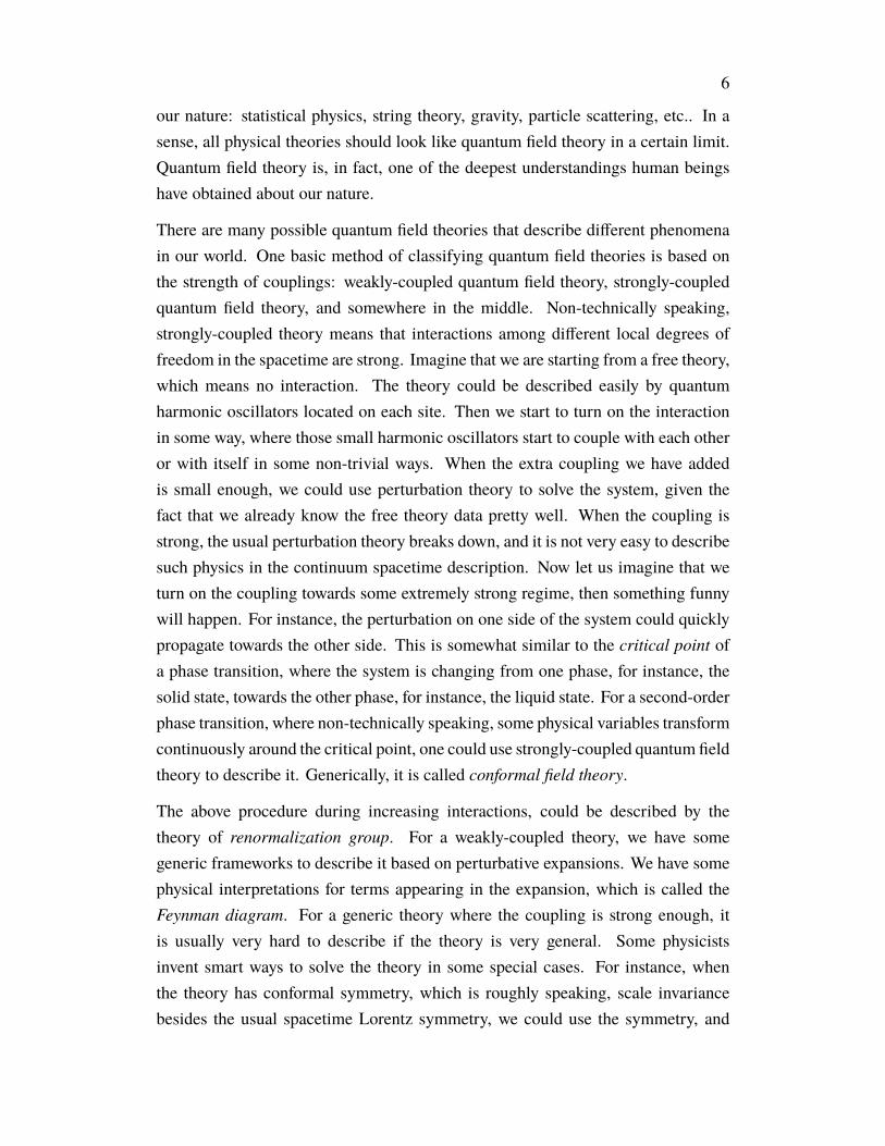
Number Page1.1 A remarkable prediction from the lattice gauge theory community.

Some light hadrons have been predicted using lattice QCD. This isfrom Figure 3 of [1]. . . . . . . . . . . . . . . . . . . . . . . . . . . 8

1.2 An artist’s creation of the quantum simulation projects of kink scat-tering [2, 3]. The depiction of characters is based entirely on theirimages in reality. From left to right: Burak Şahinoğlu, Ashley Mis-lted, Junyu Liu, John Preskill, and Guifre Vidal. Other ingredientsinclude cosmic bubbles (physical objects that are similar to kinks), aspacecraft, a cat (Schrödinger’s cat), and the Bell state. The figure iscredited to Jinglin Nicole Gao. Figures shown in the screen utilizethe figures in our scientific paper [3]. . . . . . . . . . . . . . . . . . 13

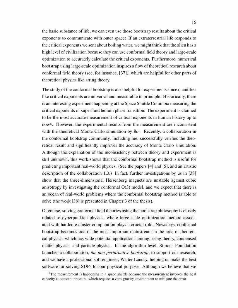
1.3 An artist’s creation about the superfluid helium conformal bootstrapproject [4] and [5]. The depiction of characters is based entirelyon their images in reality. From left to right: Shai Chester, DavidMeltzer, Junyu Liu, Walter Landry, Alessandro Vichi, David Poland,David Simmons-Duffin, and Ning Su. Other ingredients includeislands (a theoretical physics terminology referring to the isolatedregion in the theoretical space using the bootstrap method), a space-craft (referring to the Space Shuttle Columbia experiment), a diagramas stars in the sky (referring to the conformal block expansion, thebasics of the bootstrap equation in the conformal field theory). Thefigure is credited to Jinglin Nicole Gao. . . . . . . . . . . . . . . . . 16

1.4 An illustration of the string theory landscape and the swampland.This is from Figure 1 of [6]. . . . . . . . . . . . . . . . . . . . . . . 19

1.5 An imaginary plot might be made by future cyberpunkian physicists,especially high energy phenomenologists. This kind of plot includesthe required computational resource needed for observations and ex-isting computational resources provided by companies. As far as Iknow, no such plot existed until June 2021, which put together ex-perimental organizations and quantum companies. I am conjecturinghere that this type of plot will appear in the future. . . . . . . . . . . 32

xii

2.1 Black holes of maximal charge shown as a function of mass m andcharge-to-mass ratio q/m. Higher-dimension operators induce cor-rections to the extremality condition. If these corrections are positive,then theWGC is automatically satisfied (upper solid curve) since largeblack holes are unstable to decay to smaller ones. If these correctionsare negative (lower solid curve), then the WGC mandates additionallight, superextremal particles to avoid an infinite number of stableextremal black hole remnants. . . . . . . . . . . . . . . . . . . . . . 36

2.2 Constraints on higher-dimension operator coefficients derived fromblack hole entropy. The shaded regions are excluded, with the gra-dations corresponding to incremental values of ξ ∈ (0, 1/2). The leftand right panels correspond to d3 > 0 and d3 < 0, respectively. In ei-ther case, d0 < 0 is forbidden so d0 > 0 and theWGC is automaticallysatisfied. . . . . . . . . . . . . . . . . . . . . . . . . . . . . . . . . 54

3.1 The max coordinates ∆max for a collection of feasible, infeasible, andin-progress points. . . . . . . . . . . . . . . . . . . . . . . . . . . . 75

3.2 Different types of feasible points. Only the points feasible at ∆gap =∆previous are used for rescaling. . . . . . . . . . . . . . . . . . . . . . 75

3.3 Points from Figure 3.1 after rescaling. . . . . . . . . . . . . . . . . . 773.4 Points from Figure 3.3 with an adapted mesh. Points that are feasible

at ∆gap < ∆feasible have been removed. The blue spiral indicates anempty candidate cell. The other empty cells are not diagonal from afeasible cell, so they are not considered. . . . . . . . . . . . . . . . . 77

3.5 The Λ = 43 conformal bootstrap dimension island (black) comparedwith the Monte Carlo results [7, 8] (green). . . . . . . . . . . . . . . 80

3.6 Comparison between the conformal bootstrap islands atΛ = 19, 27, 35, 43projected to the ∆φ,∆s, ∆φ,∆t, and ∆s,∆t planes and theMonteCarlo results of [7, 8]. . . . . . . . . . . . . . . . . . . . . . . . . . 81

xiii

3.7 Two-dimensional projection of the results of the tiptop search atΛ = 35. The x coordinate is related to the three scalar dimensionsvia (B.8). Projections in y and z look similar. We have superimposeda convex hull encompassing the allowed points on top, obscuringsome of the disallowed points. We can see the behaviour of thetiptop algorithm, exploring the island at one ∆t4 before jumpingto a larger ∆t4 . The jumps become progressively smaller, indicatingconvergence. We computed 16 points simultaneously, and this calcu-lation took several months during which the tiptop algorithm wasbeing developed. So the points reflect occasional crashes and smallinefficiencies in the set of computed points. . . . . . . . . . . . . . . 84

3.8 Three-dimensional islands of allowed points at different∆t4 atΛ = 35,demonstrating how the islands shrink as we approach the maximum∆t4 . The x, y, and z coordinates are related to the three scalardimensions via (B.8). The values for ∆t4, from the largest regionto smallest, are 2.989, 2.99025, and 2.9905, with smaller valuesincluding all allowed points at larger values. . . . . . . . . . . . . . . 85

4.1 Cartoon showing the collapse of a false-vacuum bubble in a spinchain. The magnetization 〈Z〉 is positive in the true vacuum, butnegative in the false vacuum. A bubble-wall collision is a scatteringprocess, whichmay be (a) free (no interaction), (b) elastic (no particleproduction), or (c) inelastic (particle production). Note that in freeand elastic scattering of topological particles the left (right) particlealways remains a kink (antikink). . . . . . . . . . . . . . . . . . . . 90

4.2 Evolution of the excess energy density e (relative to vacuum), as afraction of total excess energy E , in a spin chain for two initial states:(a) created by applying a spatially smeared string operator to thevacuum and (b) constructed from MPS tensors to contain kink andantikink quasiparticle wavepackets. In (a) meson pairs are producedimmediately at the string edges, whereas in (b) there is no particleproduction until the initial kink and antikink collide. The dynamicsare restricted to a window of∼ 1000 sites, leading to boundary effectsin (a). For more details, see App. C.6. . . . . . . . . . . . . . . . . . 92

xiv

4.3 Partial phase diagrams of the extended Ising chain [9, 10], bothwithout and with a small longitudinal field h that breaks the Z2

symmetry. At h = 0, g = 1 there is a continuous (symmetry-breaking) phase transition described by the Ising CFT for λ . 0.428,and by the Tri-Critical Ising (TCI) CFT at λ ≈ 0.428. By studyingthe spin chain near to these transitions (g → 1, h → 0), we canaccess emergent, relativistic quantum field theories with confinedkinks [11, 12]. Points (i), (ii), and (iii) correspond to the data shownin the figures below. . . . . . . . . . . . . . . . . . . . . . . . . . . 94

4.4 Diagram illustrating the various types of states, and their spin pro-files, relevant for simulations. For example, our initial states arewavepackets constructed from kink-antikink pairs (a type of excitedmeson). The product states listed are eigenstates of H when g = 0,λ = 0. Away from this regime, we use MPS to accurately capturefluctuations in the vacua and excited states. . . . . . . . . . . . . . . 96

4.5 Spin expectation values and relative energy density e/E for (i) theIsing model (λ = 0, g = 0.8, h = 0.007) and (ii) the generalizedIsing model nearer to the Tricritical Ising CFT fixed point (TCI)(λ = 0.41, g = 0.98, h = 0.001). For (i), the initial wavepackets haveσ = 25 and are 248.5 sites apart (E/mµ = 3.72). For (ii), σ = 40with separation 287.4 (E/mµ = 2.62). The MPS bond dimensionsare D = 10 and D = 18 for the vacua of (i) and (ii), respectively.During the simulation the dimensions are restricted to D ≤ 128 andthe integration step size is δt = 0.05. . . . . . . . . . . . . . . . . . 102

xv

4.6 Portion of state (by probability) outside of the MPS bubble subspaceκκ(0,0) for simulations (i) and (ii) of Fig. 4.5. Here we fully accountfor momentum dependence of the basis states |κκ j,k〉 via a Fourieranalysis and count only contributions with k − j ≥ 60 (see App. C.4).For Ising (i), the small probability after the first collision of t ≈ 90indicates elastic scattering of kinks, in stark contrast with the TCIcase (ii), where the probability remains high after the first collisionat t ≈ 150. In (i), the growth of the post-collision probability withsubsequent collisions is consistent with increasingly inaccurate rep-resentation of accumulating entanglement (due to the limit imposedon the MPS bond dimension D), as well with delocalization of thewavepackets, since contributions from kink-antikink pairs with smallseparation k − j are not counted. . . . . . . . . . . . . . . . . . . . . 103

4.7 Dispersion relations (numerical, usingMPS) of kinks κ andmesons µfor λ = 0.41, g = 0.98. For mesons, energies are shown with andwithout aweak longitudinal field. Individual kinks do not have a finiteenergy for h > 0. Threshold energies for pair production are shown(computed assuming h = 0 for kinks and h = 0.001 for mesons),as is the energy (labelled Ψ) of the simulation shown in Fig. 4.5 forparameter-set (ii). . . . . . . . . . . . . . . . . . . . . . . . . . . . . 104

4.8 Spin expectation values for simulation (ii) of Fig. 4.5 at time t = 270(bond dimension D ≤ 128) after projection into selected quasiparticlesubspaces and normalization. The amount of wavefunction capturedby each (approximately orthogonal) subspace is given as a probabilityP (see App. C.4). Included subspaces are µµ, a pair of mesons oflowest energy, and κκ(a,b), a bubble made of a kink of type a and anantikink of type b (where 0 is the lowest-energy kink quasiparticle,and 1 is the next highest – see Fig. 4.7). . . . . . . . . . . . . . . . . 105

4.9 Entanglement entropy (base 2) for cuts (left-right bipartitions) of thespin chain as a function of time for the simulations (i) and (ii) ofFig. 4.5. Convergence with the bond dimension D slows as time goeson. For example, in (i) the max. cut entropy at D ≤ 128 is very likelynot converged after t ≈ 400. . . . . . . . . . . . . . . . . . . . . . . 107

xvi

4.10 Peak maximum cut entropy during the first collision as a function ofenergy (ii) close to (λ = 0.41 g = 0.98, h = 0.001) and (iii) furtherfrom the TCI point (λ = 0.3, g = 0.9, h = 0.0069), with the energycontrolled by the initial kink separation. Themesonmassmµ in latticeunits is 0.43 for (ii) vs. 0.97 for (iii), while the vacuum correlationlength ξ is 3.6 sites for (ii) and 1.8 sites for (iii), both indicating that(ii) is closer to criticality. The initial wavepacket width is σ = 40 for(ii) and σ = 19 for (iii). The kink velocity (lattice units) at the startof the first entropy jump (see Fig. 4.9) is also shown. Decreasingvelocity with energy indicates the onset of Bloch oscillations. . . . . 108

B.1 The convex hulls of the allowed points in the affine space (B.8) atderivative orders Λ = 19, 27, 35, 43. The red and black data pointsare the allowed points at derivative orders Λ = 35, 43. . . . . . . . . 146

C.1 Error made (1−〈φ j(B)|φ j(B(p))〉) in ignoring the momentum depen-dence of the tensor B used to construct MPS quasiparticle states, forboth kink andmeson excitations, for theHamiltonian parameters usedin simulations (i) and (ii) of the main text. The momentum-eigenstatefreedom on B(p) is fixed so that 〈φ j(B)|φk(B′)〉 = δ j k . . . . . . . . . 155

C.2 Estimated error (1 - infidelity per site) on momentum eigenstates|φ(B, p)〉 for kink quasiparticles, due to the choice of orthogonalityconditions on B used to achieve 〈φ j(B)|φk(B)〉 = δ j k . Here wecompare the left and right orthogonality conditions, (C.14) and (C.16).158

C.3 Spin expectation values of a kink position MPS |κ j〉 for (i) the Isingmodel and (ii) close to the Tri-Critical-Ising (TCI) point. The bonddimension is D = 8 for the Ising data, and D = 18 for the TCI data.We plot the spins for various ways of fixing the momentum-eigenstatefreedom: the left and right orthogonal conditions, (C.14) or (C.16),and the reflection-symmetric conditions (C.26), beginning from a B

tensor optimized using either the left or right conditions (since thismakes a small physical difference to the result – see App. C.3). . . . . 161

xvii

C.4 Single-kink wavepacket energy as a function of the width σ, forthe Z2-symmetric Ising model g = 0.8, λ = 0, h = 0 (in the SSBphase). We plot the energy (relative to the energy of the kink-quasiparticle momentum eigenstate) for two different ways of fixingthe momentum-eigenstate freedom on the B tensors used to con-struct the wavepacket state: an orthogonal choice 〈κ j |κk〉 = δ j k (leftand right conditions are equivalent when h = 0) and the reflection-symmetrized choice (C.26). In both cases the MPS tensors used toconstruct the state are tuned to the wavepacket momentum p = 0. . . 162

C.5 Portion of a single-kink wavepacket state outside of the single-kinksubspace κ(0) as a function of the wavepacket width σ, for the Z2-broken Ising model g = 0.8, λ = 0, h = 0.007. We plot the error fortwo different ways of fixing the momentum-eigenstate freedom onthe B tensors used to construct the wavepacket: the left orthogonalchoice 〈κ j |κk〉 = δ j k and the reflection-symmetrized choice (with B

optimized using the left orthogonal conditions). In both cases theMPS tensors used to construct the state are tuned to the wavepacketmomentum, which is p = 0. The projection into the κ(0) subspaceuses B tensors optimized using the left orthogonal conditions andfully accounts for momentum dependence via a Fourier analysis. . . . 163

C.6 Portion of the evolved bubble wavefunction outside of the kink-antikink "sector” for simulation (i) of Fig. 4.5 (λ = 0, g = 0.8,h = 0.007) at time t = 150, as a function of the minimum separationdmin := min(k − j) permitted in the two-quasiparticles basis states|κκ(0,0)j,k 〉. Probabilities are computed via a Fourier analysis, taking

into account the momentum-dependence of the basis states. Thebasis error due to interaction effects is estimated using (C.31). . . . . 169

C.7 Quasiparticle "sector” projection probabilities for simulation (ii) ofFig. 4.5 (λ = 0.41, g = 0.98, h = 0.001) at time t = 270, as a functionof the minimum separation dmin := min(k − j) permitted in the two-quasiparticles basis states | · · j,k〉. Probabilities are computed via aFourier analysis, taking into account the momentum-dependence ofthe basis states. The basis error due to interaction effects is estimatedusing (C.31). . . . . . . . . . . . . . . . . . . . . . . . . . . . . . . 170

xviii

C.8 Evolution of the energy expectation value and MPS truncation errorfor simulation (ii) of the main text. We compare different maximumbond dimensions D as well as different RK4 time-step sizes δt (forD ≤ 64), observing that the effects of the time step are most notice-able in the energy drift, whereas the bond-dimension most obviouslyaffects the truncation error at around the time of the first collision(t ≈ 150). The D ≤ 128 simulation is initialized from D ≤ 64,δt = 0.05 at t = 90. The uptick in the energy drift at t ≈ 480 is dueto unconfined wavepackets hitting the boundaries of the simulationwindow. . . . . . . . . . . . . . . . . . . . . . . . . . . . . . . . . . 173

C.9 Schmidt spectra for the maximum-entropy cut before and after thefirst collision in simulation (ii) of the main text. The bond dimensionis 128. . . . . . . . . . . . . . . . . . . . . . . . . . . . . . . . . . . 174

C.10 Evolution of spin and energy density expectation values and the cutentropy for parameter set (ii) of the main text (λ = 0.41, g = 0.98,h = 0.001), with three different initial states. State (a) is preparedby acting on the vacuum with a string operator

∏xR−1j=xL

X j , whichflips the spins to form a bubble-like state with energy E/mµ = 8.69.State (b) is similar to (a), but with the ends of the string smearedout using Gaussian packets of width σ = 40, reducing the energy toE/mµ = 4.02. State (c) is the initial state discussed in the main textwith E/mµ = 2.62, using quasiparticle wavepackets for the kinks andthe false vacuum for the middle region. The evolution parameters arethe same in all cases: The maximum bond dimension is 64 and theRK4 step size is 0.05. In (a), dramatic errors in the simulation occur att ≈ 150, indicating the difficulty of simulating these dynamics versus(b) and (c). In both (a) and (b), ballistic energy-spread emanatingfrom the initial kinks indicates that they have complex quasiparticlecontent, resulting in immediate inelastic scattering. In contrast, thetuned quasiparticle kinks of (c) do not produce appreciable ballisticspread until the bubble walls have collided. . . . . . . . . . . . . . . 176

xix

C.11 Evolution of the energy expectation value and MPS truncation errorfor the simulations of Fig. C.10. Energy drift (|1 − E(t)/E(0)|)indicates deviation from unitary evolution and results from restrictionto a maximum bond dimension of 64 as well as from numericalintegration errors (RK4 step size 0.05). Truncation error (estimatedas the maximum over cuts of the smallest Schmidt coefficient) resultsfrom the limited bond dimension and increases as entanglement isproduced. . . . . . . . . . . . . . . . . . . . . . . . . . . . . . . . . 177

C.12 Evolution of spin expectation values 〈Z〉 for a single kink in the Z2-broken Ising model, with parameters λ = 0, g = 0.4, h = 0.01. Thevacuum bond dimension is D = 6, allowed to evolve to a maximumD ≤ 32. The RK4 time-step size was δt = 0.01. . . . . . . . . . . . 178

C.13 Evolution of the position and momentum expectation values of thewavefunction of Fig. C.12 after projection onto the single-kink po-sition basis states |κ j〉. For the Hamiltonian parameters in question(see Fig. C.12), the momentum dependence of the basis states isnegligible, and could be ignored for the projection. . . . . . . . . . . 178

C.14 Evolution of the kink velocity for the single-kink simulation ofFig. C.12. Here, the velocity is computed from the projection of thewavefunction into the |κ j〉 position basis in two different ways: fromfinite-differences of the position expectation value and from the themomentum expectation value, via the numerical dispersion relationE(p). That there is a good match shows that the kink-quasiparticleansatz successfully captures the confined quasiparticles present in theZ2-broken Ising model. . . . . . . . . . . . . . . . . . . . . . . . . . 179

C.15 Momentum of the kink in simulation (i) of the main text (Ising),computed from the projected wavefunction in the κκ(0,0) basis. Thebond dimension is 128. Since the κκ(0,0) basis does not accuratelycapture the state when the kink is very close to the antikink, this datais not complete during the collision (t ≈ 90). The error bars indicatethe standard deviation of the momentum distribution. . . . . . . . . . 180

xx

C.16 Kink and antikink wavepacket velocity for the Ising model, simu-lation (i) of the main text, computed as the finite difference of theinterpolated position of the 0-intercept of 〈Z j〉. The bond dimensionis 128. Note that the data is only likely to be accurate up to t ≈ 500, assuggested by Fig. 4.9. The onset of the first collision is indicated bythe dotted line, which is the time at which the maximum cut entropybegins to grow rapidly. . . . . . . . . . . . . . . . . . . . . . . . . . 180

C.17 Kink and antikink wavepacket velocity for simulation (ii), computedas the finite difference of the interpolated position of the 0-interceptof 〈Z j〉. The bond dimension is 128. The interpretation of the 0-intercept as the position breaks down both during and, to some extent,after the collision: During the collision, the zero intercept disappearsaltogether as the kink and antikink merge and all spin expectationvalues are > 0. After the collision, there are in this case (see Fig. 4.8)at least two different bubble "branches” of the wavefunction, bothcontributing to the spin expectation values. The onset of the firstcollision is indicated by the dotted line, which is the time at whichthe maximum cut entropy begins to grow rapidly. . . . . . . . . . . . 181

C.18 Cut entropy for kink-antikink collisions, in the absence of a longitu-dinal field, with initial kink momentum p and antikink momentum−p, for three different values of p. The Hamiltonian parameters areg = 0.9, λ = 0.3, h = 0, and the wavepacket width is σ = 19.0. Thevacuum bond dimension is D = 14, with a limit D ≤ 64 imposedduring evolution. The integration time-step size was δt = 0.05. . . . 182

xxi

LIST OF TABLES

Number Page3.1 Comparison of conformal bootstrap (CB) results with previous de-

terminations from Monte Carlo (MC) simulations. We denote theleading rank-0, rank-1, rank-2, and rank-4 scalars by s, φ, t, t4, re-spectively. Bold uncertainties correspond to rigorous intervals frombootstrap bounds. Uncertainties marked with a ∗ indicate that thevalue is estimated non-rigorously by sampling points. . . . . . . . . 63

3.2 Comparison of field theory results using various techniques: fixed-dimensional expansion in three dimensions (d = 3 exp), epsilonexpansion (ε-exp) and high temperature expansion (HT). We denotethe leading rank-0, rank-1, rank-2, and rank-4 scalars by s, φ, t, t4, re-spectively. Another estimate of∆t in the fixed-dimensional expansioncan be found in [13] in terms of the crossover exponents φT = Y2ν,with Y2 = 3 − ∆t . We do not report it here because the errors dependon the value of ν used. . . . . . . . . . . . . . . . . . . . . . . . . . 67

3.3 Four-point function configurations that give independent crossingequations under equating their s- and t-channels, along with whethereven or odd spins `± appear for each irrep in each channel, and thenumber of crossing equations that each configuration yields. . . . . . 72

B.1 Parameters used for the computations of the conformal bootstrapislands in section 3.4. The sets SΛ are defined in (B.1). . . . . . . . . 141

B.2 Parameters used for the optimization computations in section 3.4.The set S35 is defined in (B.1). . . . . . . . . . . . . . . . . . . . . . 141

B.3 Allowed points in the Λ = 43 island. . . . . . . . . . . . . . . . . . . 147B.4 Disallowed points computed at Λ = 43. . . . . . . . . . . . . . . . . 148B.5 Allowed points in the Λ = 43 island used to obtain bounds on λφφs,

CT , and CJ , along with the gaps above ∆T and ∆J that were assumed. 148

1

C h a p t e r 1

INTRODUCTION: ASPECTS OF "CYBERPUNKIAN"QUANTUM FIELD THEORY

1.1 Space opera and CyberpunkMaybe a good way to start this thesis is through science fiction. Generically,there are many ways to classify science fiction stories1. One example is throughthe contents. If a science fiction story is mainly talking about interstellar wars,outer-space civilizations, and spacetime traveling, it is usually called "space opera".If a science fiction story is mainly talking about the relationships among digitaltechnologies, robots, and humans, it is called "cyberpunk"2,3.

As one of the most important subgenres, space opera has a longer history. Currently,some people believe that it originally appeared in some American magazines in the1920s. After people understand much better about our universe during and after thewars, space operas have been significantly developed, especially around the ColdWar. On the other hand, cyberpunkian stories are relatively new. They have beenwidely created and discussed after people realize the potential of digital technologies,computer science, and the Internet. If I am allowed to choose two representativesfor those two subgenres, I wish to choose the film series Star Wars by George Lucasfor space opera, and the novel Do Androids Dream of Electric Sheep? by PhilipDick for cyberpunk4.

Science, a systematic and fundamental understanding of the nature, and sciencefiction, a fantastic imagination of how science and technology could change humansociety in the future, might be closely related to the development of human societyitself. I firstly start to understand this when I read the lecture notes, Nature andthe Greeks and Science and Humanism by Erwin Schrödinger [14], who partiallyexpresses similar feelings from my understanding. During the Cold War, with the

1The classification is in the non-academic sense. For a long time, science fiction novels are notrecognized in the mainstream of literature.

2There are some other topics, for instance, Steampunk. Another more common way to classifyscience fiction is through hard or soft science fiction, referring to roughly speaking if the story ismore scientific or more literary.

3Sometimes, cyberpunk describes an icy future world ruled by technology with a flavor ofdystopia. However, we hope to use a broader definition of cyberpunk, that in the possible future,humanity will coexist in harmony with high technology.

4The film version of it, directed by Ridley Scott in 1982, is the celebrated Blade Runner.

2

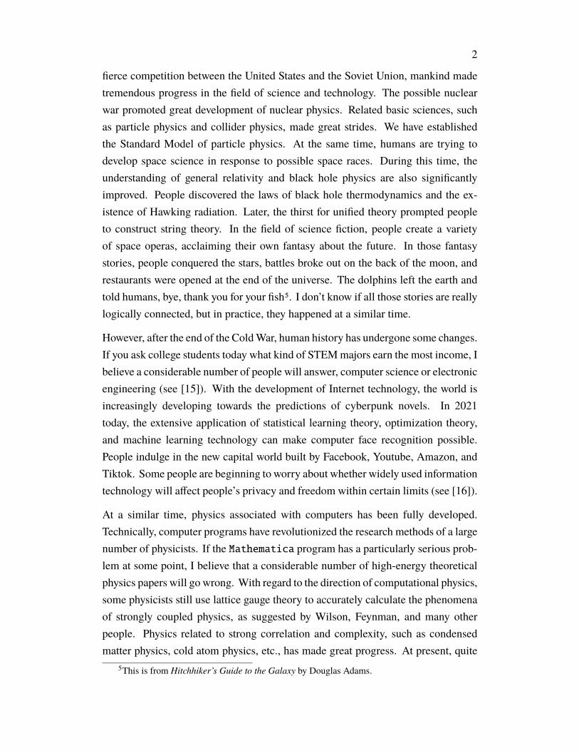
fierce competition between the United States and the Soviet Union, mankind madetremendous progress in the field of science and technology. The possible nuclearwar promoted great development of nuclear physics. Related basic sciences, suchas particle physics and collider physics, made great strides. We have establishedthe Standard Model of particle physics. At the same time, humans are trying todevelop space science in response to possible space races. During this time, theunderstanding of general relativity and black hole physics are also significantlyimproved. People discovered the laws of black hole thermodynamics and the ex-istence of Hawking radiation. Later, the thirst for unified theory prompted peopleto construct string theory. In the field of science fiction, people create a varietyof space operas, acclaiming their own fantasy about the future. In those fantasystories, people conquered the stars, battles broke out on the back of the moon, andrestaurants were opened at the end of the universe. The dolphins left the earth andtold humans, bye, thank you for your fish5. I don’t know if all those stories are reallylogically connected, but in practice, they happened at a similar time.

However, after the end of the ColdWar, human history has undergone some changes.If you ask college students today what kind of STEMmajors earn the most income, Ibelieve a considerable number of people will answer, computer science or electronicengineering (see [15]). With the development of Internet technology, the world isincreasingly developing towards the predictions of cyberpunk novels. In 2021today, the extensive application of statistical learning theory, optimization theory,and machine learning technology can make computer face recognition possible.People indulge in the new capital world built by Facebook, Youtube, Amazon, andTiktok. Some people are beginning to worry about whether widely used informationtechnology will affect people’s privacy and freedom within certain limits (see [16]).

At a similar time, physics associated with computers has been fully developed.Technically, computer programs have revolutionized the research methods of a largenumber of physicists. If the Mathematica program has a particularly serious prob-lem at some point, I believe that a considerable number of high-energy theoreticalphysics papers will go wrong. With regard to the direction of computational physics,some physicists still use lattice gauge theory to accurately calculate the phenomenaof strongly coupled physics, as suggested by Wilson, Feynman, and many otherpeople. Physics related to strong correlation and complexity, such as condensedmatter physics, cold atom physics, etc., has made great progress. At present, quite

5This is from Hitchhiker’s Guide to the Galaxy by Douglas Adams.

3

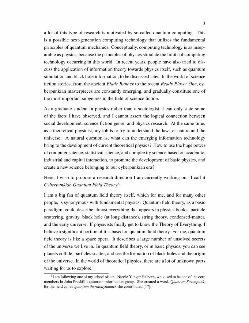
a lot of this type of research is motivated by so-called quantum computing. Thisis a possible next-generation computing technology that utilizes the fundamentalprinciples of quantum mechanics. Conceptually, computing technology is as insep-arable as physics, because the principles of physics stipulate the limits of computingtechnology occurring in this world. In recent years, people have also tried to dis-cuss the application of information theory towards physics itself, such as quantumsimulation and black hole information, to be discussed later. In the world of sciencefiction stories, from the ancient Blade Runner to the recent Ready Player One, cy-berpunkian masterpieces are constantly emerging, and gradually constitute one ofthe most important subgenres in the field of science fiction.

As a graduate student in physics rather than a sociologist, I can only state someof the facts I have observed, and I cannot assert the logical connection betweensocial development, science fiction genre, and physics research. At the same time,as a theoretical physicist, my job is to try to understand the laws of nature and theuniverse. A natural question is, what can the emerging information technologybring to the development of current theoretical physics? How to use the huge powerof computer science, statistical science, and complexity science based on academic,industrial and capital interaction, to promote the development of basic physics, andcreate a new science belonging to our cyberpunkian era?

Here, I wish to propose a research direction I am currently working on. I call itCyberpunkian Quantum Field Theory6.

I am a big fan of quantum field theory itself, which for me, and for many otherpeople, is synonymous with fundamental physics. Quantum field theory, as a basicparadigm, could describe almost everything that appears in physics books: particlescattering, gravity, black hole (at long distance), string theory, condensed-matter,and the early universe. If physicists finally get to know the Theory of Everything, Ibelieve a significant portion of it is based on quantum field theory. For me, quantumfield theory is like a space opera. It describes a large number of unsolved secretsof the universe we live in. In quantum field theory, or in basic physics, you can seeplanets collide, particles scatter, and see the formation of black holes and the originof the universe. In the world of theoretical physics, there are a lot of unknown partswaiting for us to explore.

6I am following one of my school sisters, Nicole Yunger Halpern, who used to be one of the coremembers in John Preskill’s quantum information group. She created a word, Quantum Steampunk,for the field called quantum thermodynamics she contributed [17].

4

When I use the term cyberpunk, I want to distinguish it from common vocabulary,the so-called computational physics. Beyond traditional terminology, I hope toemphasize that cyberpunk quantum field theory can be based on the followingtwo aspects. First, cyberpunkian science prefers to use information theory andtechnology that are cutting-edge and even under development, for instance, machinelearning, optimization problems, applied mathematics and statistics, and quantumcomputing. Secondly, I hope that cyberpunkian physics is not only practical, butalso theoretically helpful to physics itself, or even vice versa. Just as superstringtheory expert Edward Witten does for the mathematical community, we could alsousing physics theory to guide possible computer science discoveries.

In the following discussion, I hope to describe the possible prospects of this science.Of course, technically, these stories are already happening. The Large HadronCollider (LHC) operating in Europe is constantly usingmachine learning algorithmsto process data on particle collisions. Dark matter detection satellites operating inthe sky will also cooperate with companies in industry to deal with scientific issuesof interest (see for instance [18]). However, as a theoretical physicist, I hope that inthe future, people will be able to do more in-depth research on theoretical physicsissues related to cutting-edge information technology. At least, I think this formspart of physical science in our generation.

In the following discussion, I will use the following three simple examples todemonstrate that cyberpunkian quantum field theory may become an important andeffective science. It includes quantum simulation of quantumfield theory, large-scaleoptimization of conformal field theory, and discussion of the relationship betweenquantum field theory landscape and big data science. I will also do a simple non-technical discussion of quantum field theory, and a simple outlook on this relatedissue, including black hole thought experiment and quantum information science,It from qubit and the non-perturbative bootstrap, Church-Turing Thesis, ComputerScience(CS)-inspired physics and physics-inspired CS, possible future of classicaland quantum technology, and finally, companies and colliders.

As a science fiction lover, I often think about such problems. What will the scienceI do look like in two hundred or one thousand years? Will it still be meaningful?From scholasticism to modern science, we take nearly three hundred years. Thepopularity of the internet is what happened in the past three decades. What will theworld look like in two thousand years? Will the banking industry be completelychanged by quantum computing? Will humans make a collider as big as the Milky

5

Way? Will the military use Higgs particles as weapons?

Wring this thesis, in a sense, is to expressmy sincere respect for some great scientists.Lev Landau, Enrico Fermi, Richard Feynman, StevenWeinberg, KenWilson, Chen-Ning Yang, Steven Hawking, Edward Witten, Alexander Zamolodchikov, etc., andnowadays in our quantum era, Alexei Kitaev and John Preskill. They establishedthe deepest human understanding of the universe during those prosperous years, anddefines the science of our time. I think that the current status of physics has givenme some opportunities for fledgling young people. To me, traditional physicistsare like hackers. They discovered the secrets of this world through various means.Cyberpunkian physicists seem to try to build a completely new, Turing-completeworld. For me, they are all important sciences. Maybe one day, when people canfind a variety of new particles on the collider, reach the boundary of the black holehorizon, or freely edit topological quantum qubits, some of them will think that,what we are doing currently, are treasures.

1.2 Quantum field theoryIn order to discuss cyberpunkian quantum field theory, I will first introduce whatquantum field theory is. Here I will provide a non-technical introduction to quantumfield theory.

So what is quantum field theory? A possible generic description is that it is aquantum formulation of continuum physics in the spacetime. Consider that we havecomplicated interactions among some atoms and molecules placed discretely in thespacetime. There are physical laws governing the forces, for instance, the Van derWaals force. However, if we feel it is too complicated to keep track of interactions ofall particles, we could zoomout and askwhat the emergent description iswhenwe arelooking at a length scale that is much larger than the lattice spacing. Sometimes weare able to arrive at a beautiful emergent description, for instance, if those moleculesform a liquid, which is called hydrodynamics. In this case, hydrodynamics is afield theory. When the full procedure is treated quantumly, for instance, if we areconsidering some interacting quantum harmonic oscillators, the description is calledquantum field theory, where we are assuming that there are an infinite number ofquantum harmonic oscillators located in a continuum spacetime.

A deep interpretation between the lattice model and the quantum field theory de-scription is given by Ken Wilson, and the above process is called renormalization.People find that the renormalization process occurs in almost all phenomena in

6

our nature: statistical physics, string theory, gravity, particle scattering, etc.. In asense, all physical theories should look like quantum field theory in a certain limit.Quantum field theory is, in fact, one of the deepest understandings human beingshave obtained about our nature.

There are many possible quantum field theories that describe different phenomenain our world. One basic method of classifying quantum field theories is based onthe strength of couplings: weakly-coupled quantum field theory, strongly-coupledquantum field theory, and somewhere in the middle. Non-technically speaking,strongly-coupled theory means that interactions among different local degrees offreedom in the spacetime are strong. Imagine that we are starting from a free theory,which means no interaction. The theory could be described easily by quantumharmonic oscillators located on each site. Then we start to turn on the interactionin some way, where those small harmonic oscillators start to couple with each otheror with itself in some non-trivial ways. When the extra coupling we have addedis small enough, we could use perturbation theory to solve the system, given thefact that we already know the free theory data pretty well. When the coupling isstrong, the usual perturbation theory breaks down, and it is not very easy to describesuch physics in the continuum spacetime description. Now let us imagine that weturn on the coupling towards some extremely strong regime, then something funnywill happen. For instance, the perturbation on one side of the system could quicklypropagate towards the other side. This is somewhat similar to the critical point ofa phase transition, where the system is changing from one phase, for instance, thesolid state, towards the other phase, for instance, the liquid state. For a second-orderphase transition, where non-technically speaking, some physical variables transformcontinuously around the critical point, one could use strongly-coupled quantum fieldtheory to describe it. Generically, it is called conformal field theory.

The above procedure during increasing interactions, could be described by thetheory of renormalization group. For a weakly-coupled theory, we have somegeneric frameworks to describe it based on perturbative expansions. We have somephysical interpretations for terms appearing in the expansion, which is called theFeynman diagram. For a generic theory where the coupling is strong enough, itis usually very hard to describe if the theory is very general. Some physicistsinvent smart ways to solve the theory in some special cases. For instance, whenthe theory has conformal symmetry, which is roughly speaking, scale invariancebesides the usual spacetime Lorentz symmetry, we could use the symmetry, and

7

some other internal constraints to partially, or even completely, solve the theory[19]. One could try some other similar strategies when the theory is integrable,namely, when it contains infinite number of conserved charges [20]. When thetheory is supersymmetric, sometimes one could do perturbative expansions easierbecause in this case the Feynman diagramsmight have some cancellations andmaybeone could use it to solve part of non-perturbative physics. Some other methods, forinstance, the duality between weakly-coupled gravitational theories and strongly-coupled quantum field theories without gravity, which is called holography or theAdS/CFT (Anti-de Sitter Space/Conformal Field Theory) correspondence (we willmention it later) [21], might shed light on solving strongly-coupled quantum fieldtheories. All of them are still active research directions in theoretical physics.

However, people still don’t have a very good understanding of strongly-coupledquantum field theory in general. For instance, the strongly coupled regime ofquantum chromodynamics(QCD) is still not clearly understood, even if we have theabove theoreticalmethods at hand. One couldmeasure several properties of strongly-coupled QCD in some low energy colliders, and it is extremely hard to predict somebound states using theoretical calculations from quantum field theories. The Yang-Mills existence and mass gap problem defined as one of the Millennium PrizeProblems is also about field theories beyond the weakly-coupled regime, and it isstill an open problem even without a very precise mathematical definition. The high-temperature superconductivity phenomenon might also admit a low energy effectivefield theory description around the critical point of their phase diagrams, but it isstill far from a very concise formulation and a reasonable prediction. I probablycould list many problems of this type, involving theoretical understandings andphenomenological predictions of quantum field theories. All of them are closelyrelated to the universe we live in, and all of them seem challenging. Maybe forsome people, it is fair to say that we still don’t understand quantum field theories,although it is already at least half a century after its birth.

Another particularly important example is string theory, which is a candidate fora consistent theory that could describe everything appearing in this world, fromquantum black holes, big bang physics, to subatomic, atomic, andmolecular physics.String theory itself could be formulated in a quantum field theory manner. Inparticular, quantum black holes could also be understood as a specific strongly-coupled quantum field theory phenomenon. If we address the weakly-coupled limit,one could compute graviton exchange in a semiclassical fashion of quantum field

8

0

500

1000

1500

2000

M[M

eV

]

p

K

rK* N

LSXD

S*X*O

experiment

width

input

QCD

Figure 1.1: A remarkable prediction from the lattice gauge theory community.Some light hadrons have been predicted using lattice QCD. This is from Figure 3 of[1].

theory in the curved spacetime, which is called gravitational waves.

Okay, so some people may say that if pure theoretical methods fail, why we don’t trynumerics? This is a very fair statement, and yes, we have already tried. Ken Wilsonand other people suggest that maybe we could solve strongly-coupled quantum fieldtheories by making a lattice regularization. That is, trying to discretize your spacein a lattice. One could try to solve the theory in the lattice, and take some reasonablelimits towards the continuum. For gauge theories used in particle physics, thissubject is usually called the lattice gauge theory.

Nowadays, the idea about regularizing field theories in a lattice has made significantprogress. In Figure 1.1, where I am quoting Figure 3 of [1], people could matchsome experimental observations about the light hadron spectrum with QCD by afirst-principle calculation. It agrees very well! This type of agreement could notonly show powerful predictability of quantum field theories but also show the factthat nature is a good computer!

However, despite its glorious success, there are several fundamental limitations tothe current algorithms. The main problem is that, in principle, quantum field theorycontains an infinite large Hilbert space on each site located in the spacetime. Thisdemands a huge amount of computational resources! Here, I am claiming that,in order to solve more important problems, we have to be smarter: the numerical

9

challenge we face on simulating and predicting quantum field theories forces usto use the most cutting-edge methods from information technology, while somenovel, fundamental understanding of quantumfield theories and fundamental physicsthemselves will come from computer science, classical or quantum. This is the placewhere cyberpunkian physicists should go.

In the following discussions, I will mainly describe three cyberpunkian researchdirections I have worked on: simulating quantum field theories using quantumdevices, conformal field theory and large-scale optimization, and string theoryversus data science. Later, I will discuss some general comments about fundamentalphysics and information technology.

1.3 Simulating quantum field theory using quantum devicesGoing back to the story of lattice gauge theory, here I am pointing out some dif-ficulties in solving quantum field theories by putting them in a lattice only with aclassical computer and brute force methods.

The first problem is the computational power. Lattice quantumfield theory has a verylarge Hilbert space. In principle, we have a continuum number of sites located in thespacetime, while each site has an infinite Hilbert space dimension. By truncatingthe local Hilbert space and choosing a cutoff for lattice spacing, we are able to solvethe theory in a finite, but large, Hilbert space dimension, with proper treatment ofan extrapolation of numerical results towards the continuum. This is a very highcomputational cost. Firstly, it is extremely hard to do it naively using the way ofexact diagonalization, namely, diagonalize a large Hamiltonian directly. Secondly,one could try to measure some correlation functions using random algorithms, forinstance, some versions of Monte Carlo methods. This is usually cheaper thanexact diagonalization, but it is still hard to operate due to a large number of sitesand a large number of configurations to sample. The second problem is the signproblem. For fermionic theories, when we compute some predictions using MonteCarlo method by doing some samplings of path integrals, we will often encounteroscillating amplitudes, making the result hard to converge. Those problems havechallenged the current lattice gauge theory community for a long time, and peoplefind that it is extremely hard to make predictions, for instance, for real-time physics.

Thus, in order to solve quantum field theory in general, especially for strongly-coupled theory in a lattice, one might consider some potential future computationaldevices. One could imagine that the computation could be done in a quantum

10

computer, which could simulate physical process of quantum field theory itself. Ifind that many quantum computing people like to quote what Richard Feynman saidin his paper [22], and I am happy to quote it again:

. . . trying to find a computer simulation of physics, seem to me to be anexcellent program to follow out.. . . and if you want to make a simulation ofnature, you’d better make it quantummechanical, and by golly it’s a wonderfulproblem, because it doesn’t look so easy.

Richard Feynman is, at least partially, a particle theorist. In fact, as indicated fromhis paper [22], it seems that one of the earliest motivations for quantum computingis to simulate quantum field theories. (See a review article given by John Preskill[23].)

Nowadays, in 2021, quantum computing becomes one of the most exciting scientificareas, receiving significant attention from academia, industry, government, and thewhole society. John Preskill [24] announced that nowadays we are living in aquantum era which is called NISQ (Noisy Intermediate-Scale Quantum), where aquantum computer with 50-100 qubits may be able to perform tasks that exceedthe capabilities of today’s classical digital computers, but the noise of quantumgates will limit the size of quantum circuits that can be reliably executed. Infact, Google already claims that they have achieved quantum supremacy, that is,quantum computers can accomplish tasks that classical computers cannot [25].For simulating quantum field theories themselves, quantum computing methodscould provide certain advantages against two main problems I have mentionedbefore for simulating quantum field theory in a classical computer. Firstly, quantumcomputing is proceeded by quantum states made by qubits, and unitary evolutionmade by unitary operators acting on the Hilbert space. Roughly speaking, the spaceit contains, is naturally, exponentially large than classical computation. Secondly,quantum computing is able to solve the sign problem naturally [26], which mightpotentially remove the sign problem difficulty appearing in the fermionic quantumMonte Carlo simulation.

One early remarkable quantum algorithm to simulate quantum field theories is calledthe Jordan-Lee-Preskill algorithm (see the original papers [27, 28], and a series ofrelated papers [29, 30]). This type of algorithm contains state preparation, timeevolution, and measurement of some specific quantum field theory tasks happeningat strong coupling. One could also associate the above algorithm into some certain

11

complexity classes [30]. This algorithm, especially the time evolution of the quan-tum field theory Hamiltonian, is shown to be polynomial in system size, sharpeningthe potential quantum advantage for simulating quantum field theories in quantumcomputers.

In the above framework, simulating quantum field theories could be generally re-garded as simulating some specific Hamiltonians. Thus, it is natural to utilizemethods from general Hamiltonian simulations developed by the quantum algo-rithm community. When simulating a quantum Hamiltonian, one could roughlyclassify quantum simulation algorithms in the following three types: digital, ana-log, and variational quantum simulation. The above Jordan-Lee-Preskill algorithmis a typical algorithm for digital simulation, where we assume a possible universalquantum computer when we are constructing the algorithm. For analog simulation,the algorithm is developed by constructing an actual Hamiltonian in the cold-atomiclab, for instance, the Hamiltonian made by Rydberg atoms. Variational algorithmsare somehow in the middle: it will make use of variational methods, only coveringa subset of the whole Hilbert space. Variational algorithms might be constructedin a hybrid quantum-classical way, which is made suitable for near-term quantumdevices. All of them are potentially useful for simulating quantum field theories.

When constructing quantum simulation algorithms or actually doing simulationsin a quantum computer or in the lab, classical simulation might play an importantand specific role. Firstly, quantum-classical hybrid algorithms are widely used.Especially in the near-term, quantum algorithms are only helpful to speed up cal-culations in certain steps in a whole classical algorithm. Those classical piecesmay not be replaceable. Secondly, classical algorithms might be helpful to findlimitations of classical computations, and understand conceptually and technicallywhere quantum algorithms might play a role. Here I wish to mention specificallytwo types of algorithms: matrix product state (MPS) algorithms and semidefiniteprogramming (SDP) algorithms. Of course, both of those algorithms have verywide applications that are even beyond the scope of physics. MPS algorithms arehelpful for identifying some low energy states of quantummany-body systems in the1+1 dimension, which could have emergent field theory behaviors around criticalpoints. SDP algorithms are basics of convex programming that are widely used inoperations research and optimization, which are also basic algorithms for solvinghigher-dimensional conformal field theories numerically (we will describe this inmore detail in the next section). Both of them are important classical algorithms. It

12

is important to understand their advantages and limitations comparing to quantumcomputation, where quantum field theories are perfect playgrounds to test them.

I also wish to mention here part of my own contributions. With one of my ad-visors, John Preskill, I have been exploring quantum simulation of domain wallscattering in 1+1 dimensional quantum field theories. Domain walls, or kinks, inthe 1+1 dimensional scalar field theories, are the simplest examples of topologicaldefects. They are like walls splitting two different field configurations in the theory.The existence of domain walls is closely related to vacuum decay in cosmology,sharpening its relevance to the real world. Historically, there are many authors whostudied kinks in quantum field theories at weak or strong coupling (for instance,[31, 32]), but strongly-coupled kinks are extremely hard to solve at strong-couplingfor non-integrable, 1+1 dimensional quantum field theories. In the work with JohnPreskill and Burak Şahinoğlu, we are trying to construct theoretical algorithms tosimulate scattering process of kinks, while in the work with Ashley Milsted, JohnPreskill and Guifre Vidal, we are trying to study analog models in spin chains andsimulate the kink scattering process in the MPS approximation [2, 3]. (see Figure1.2 for an artistic illustration. The work [3] is presented in Chapter 4 of the thesis)

Simulating quantum field theories are generically helpful for studying quantum fieldtheories appearing in the formal high energy theory community, for instance, theorieswith supersymmetry, in higher dimensions or containing gravitational sectors. Onepossible ambitious goalmight be studying large-N supersymmetric gauge theory andtrying to verify Maldacena’s conjecture about the AdS/CFT correspondence [21].It might also be helpful for studying high energy phenomenology, experimentsor observations, for instance, solving QCD in the strongly-coupled regime. Thosestudies might also benefit the community of quantum algorithms, which will providenovel, clear tasks, cool applications, and good targets for benchmarks. Finally, itmight be helpful for conceptual understanding of quantum simulation in our physicalworld, namely, the Church-Turing Thesis. We will discuss those issues later.

1.4 Conformal field theory and large-scale optimizationIn this section, we will move to another topic that is more related to classicalcomputation instead of quantum. That is, conformal bootstrap and its relation tolarge-scale optimization.

We discuss before the concept conformal field theory, which appears in some sta-tistical models as a low energy effective description around the second-order phase

13

Figure 1.2: An artist’s creation of the quantum simulation projects of kink scattering[2, 3]. The depiction of characters is based entirely on their images in reality. Fromleft to right: Burak Şahinoğlu, Ashley Mislted, Junyu Liu, John Preskill, and GuifreVidal. Other ingredients include cosmic bubbles (physical objects that are similarto kinks), a spacecraft, a cat (Schrödinger’s cat), and the Bell state. The figure iscredited to Jinglin Nicole Gao. Figures shown in the screen utilize the figures in ourscientific paper [3].

transition. Around the critical point of some statistical models, partially because ofthe scale invariance, the spacetime symmetry of the theory has been extended fromthe usual rotational or Lorentzian symmetry towards a larger symmetry: conformalsymmetry7. Such a theory might be a little counter-intuitive: one could make atransformation from the far infinity to the origin of the coordinate system, and theaction of the theory is still invariant. Thus, conformal field theories are used todescribe violent behaviors around the critical point, which experiences a drasticchange between different two phases. The behavior is universal, which means thatmultiple microscopic models might correspond to the same conformal field theory.The low energy spectra of conformal field theories will provide some universal num-bers that are measurable in the statistical system, which are called critical exponents.Thus, multiple microscopic models might share the same critical exponents. Onestandard example is that the phase transition of the boiling water shares the same

7Although there are still some technical differences between scale invariance and conformalinvariance.

14

universality class with the 3d Ising model, a model made by physicists to describethe dynamics of magnets. Because of universality, conformal field theory is a verygeneric concept that could be applied in many places that admit second-order phasetransitions. Moreover, conformal field theory technologies are directly applicableto string theories, since the worldsheet theory of string theories is conformallyinvariant.

Non-trivial conformal field theories are typical strongly-coupled quantum field the-ories, making them very hard to solve. However, conformal invariance stronglyconstraints the behaviors of the theory. For instance, some correlation functionsare directly constrained as some specific forms. Some people believe that confor-mal field theories, and some other strongly-coupled field theories, are fragile in thefollowing sense. These theories are like precise gears: as long as few conditionsare input, the strong limitation of conformal symmetry will isolate or even uniquelydetermine these theories. This philosophy of understanding quantum field theoryis called bootstrap, a possible way of understanding strong coupling without reallyquantize those theories from classical actions.

The bootstrap philosophy in particle physics is studied widely in some certain timescales around the last century (for instance, [33, 34]), but quickly decays with manyopen problems unsolved, replaced by related studies about QCD. However, recently,the idea of bootstrap in field theories has returned to be a hot topic in the highenergy physics community, since we become more cyberpunkian. People noticethat one could solve bootstrap equations, the consistency equations appearing instrongly-coupled quantum field theories, by optimization technics. For instance,bootstrap equations in conformal field theories are identities where a sum overcontributions from different sectors of the theory is equal to zero, which looks likea hyperplane in some higher dimensional Euclidean spaces. Roughly speaking, thehyperplane could be located by finding some other optimal hyperplanes cutting thespace towards small pieces, while themethods for finding optimal planes are standardin optimization and operations research: the semidefinite programming (SDP). Themodern technologies of computer science allow people to work on optimizationproblems numerically at large scale, making numerical bootstrap possible (see asummary by [19, 35]). In fact, conformal bootstrap holds theworld record for solvingthe most digests of the Holy Grail problem in statistical physics: determining thecritical exponents for the 3d Ising model [36]. Considering the fact that the 3d Isingmodel shares the same critical exponents with the boiling water, and that water is

15

the basic substance of life, we can even use those bootstrap results about the criticalexponents to communicate with outer space: If an extraterrestrial life responds tothe critical exponents we sent about boiling water, we might think that the alien has ahigh level of civilization because they can use conformal field theory and large-scaleoptimization to accurately calculate the critical exponents. Furthermore, numericalbootstrap using large-scale optimization inspires a flow of theoretical research aboutconformal field theory (see, for instance, [37]), which are helpful for other parts oftheoretical physics like string theory.

The study of the conformal bootstrap is also helpful for experiments since quantitieslike critical exponents are universal and measurable in principle. Historically, thereis an interesting experiment happening at the Space Shuttle Columbia measuring thecritical exponents of superfluid helium phase transition. The experiment is claimedto be the most accurate measurement of critical exponents in human history up tonow8. However, the experimental results from the measurement are inconsistentwith the theoretical Monte Carlo simulation by 8σ. Recently, a collaboration inthe conformal bootstrap community, including me, successfully verifies the theo-retical result and significantly improves the accuracy of Monte Carlo simulation.Although the explanation of the inconsistency between theory and experiment isstill unknown, this work shows that the conformal bootstrap method is useful forpredicting important real-world physics. (See the papers [4] and [5], and an artisticdescription of the collaboration 1.3.) In fact, further investigations by us in [38]show that the three-dimensional Heisenberg magnets are unstable against cubicanisotropy by investigating the conformal O(3) model, and we expect that there isan ocean of real-world problems where the conformal bootstrap method is able tosolve (the work [38] is presented in Chapter 3 of the thesis).

Of course, solving conformal field theories using the bootstrap philosophy is closelyrelated to cyberpunkian physics, where large-scale optimization method associ-ated with hardcore cluster computation plays a crucial role. Nowadays, conformalbootstrap becomes one of the most important mainstream in the area of theoreti-cal physics, which has wide potential applications among string theory, condensedmatter physics, and particle physics. In the algorithm level, Simons Foundationlaunches a collaboration, the non-perturbative bootstrap, to support our research,and we have a professional soft engineer, Walter Landry, helping us make the bestsoftware for solving SDPs for our physical purpose. Although we believe that we

8The measurement is happening in a space shuttle because the measurement involves the heatcapacity at constant pressure, which requires a zero-gravity environment to mitigate the error.

16

Figure 1.3: An artist’s creation about the superfluid helium conformal bootstrapproject [4] and [5]. The depiction of characters is based entirely on their imagesin reality. From left to right: Shai Chester, David Meltzer, Junyu Liu, WalterLandry, Alessandro Vichi, David Poland, David Simmons-Duffin, and Ning Su.Other ingredients include islands (a theoretical physics terminology referring to theisolated region in the theoretical space using the bootstrap method), a spacecraft(referring to the Space Shuttle Columbia experiment), a diagram as stars in the sky(referring to the conformal block expansion, the basics of the bootstrap equation inthe conformal field theory). The figure is credited to Jinglin Nicole Gao.

are currently using the most cutting-edge optimization results from the operationsresearch community [39], the current algorithms still have an opportunity for po-tential significant improvement. We also wish to mention that SDP is an extremelyuseful algorithm that admits a large quantum speedup. Thus, conformal bootstrapmight potentially provide clear physical applications for the quantum SDP solver,and will be helpful for benchmarking quantum algorithms and devices [40].

1.5 The theoretical landscape and data scienceIn this section, I wish to comment on the landscape of quantum field theories andits relation to data science.

Quantum field theory (or the whole fundamental theoretical physics), at least formany people, including me, is an extremely difficult subject. Theorists have con-structed a large number of quantum field theories, which describe some generalphenomena in this world or a certain universe. Some theories live in high dimen-

17

sions or some highly-curved spacetime that humans cannot easily understand. Thevarious counter-intuitive phenomena appearing in the strongly-coupled theory makeit more difficult for physicists to control. Some quantum field theories cannot evenbe precisely definedmathematically. Moreover, quantum field theory can havemanyparameters and many possible descriptions, which may lead to the same or differentpredictions. I think, at least for me, many problems cannot be thoroughly studiedin my whole life. If I am supposed to give a name for the space of quantum fieldtheories, I will call it the landscape, a common term used by high energy physicists.

Another difficulty of quantumfield theory lies in its experimental difficulty. Probablythe best way to verify quantum field theory in the subatomic world is various high-energy physics experiments, especially collider experiments. Experimental resultsfrom colliders could verify or expand predictions from some quantum field theoriesby colliding subatomic particles at some certain energies. This is an extremelycomplicated process. From the various nuclear resonance states of the low energycollider to the hadron jet on the hadron collider, physics involved in those processesis very difficult to calculate and measure. This often requires a huge amount ofengineering and the efforts of countless researchers to achieve.

Perhaps physicists should thank themselves for being in this cyberpunk era. Thefamous hadron collider, LHC, generates a lot of data every day. A considerablepart of the data will be processed by professional data scientists or particle physi-cists. Therefore, big data science is an important means of contemporary particlephysics research. For example, machine learning is becoming an important meansof processing experimental data of particle physics. In terms of phenomenologicaltheories that are closer to experimental observations, data science has also graduallybecome an important way to explore the predictions brought by different effectivefield theories and Wilson parameters, or to simulate experimental data to recon-struct particle resonance states. I here cite two related works on experiment andphenomenology [41, 42]. Interested readers can easily find more works on theInternet.

Here, I prefer to discuss a story that is mainly about formal high energy theory.Perhaps themost sophisticated networks of quantumfield theories are constructed bystring theorists. String theory itself could also be understood as a paradigm adaptingnumerous quantum field theory descriptions. One way to quantify the complexity ofstring theory is to count its vacua. In some simplest quantummechanical models, weare familiarwith, for instance, hydrogen atomswithCoulomb’s force, the degeneracy

18

of the vacuum states is usually very few. However, there is potentially a very largeamount of vacuum degeneracy in string theory. There are so many choices ofmicroscopic theory, compactification manifold, bundle or brane configuration, flux,etc. Some people believe that the total number of string theory vacua might befinite, and the estimate is usually huge numbers, for instance, 10500 (see some earlypapers, [43–45]).

The gigantic possible choices of string theory vacua seem leading to many differentpossibilities of physical predictions, for instance, different realizations of effectivefield theories at low energies, and different possibilities of constants appearing inour universe, for instance, the mass of the electron. The physical interpretation ofthe string theory landscape and its possible relationship with some illegal theorieswhich could not correspond to any realizations of quantum gravity, are still openproblems. People call those the collection of illegal theories the swampland.

The study of string theory landscape and the swampland is a very difficult subject,partially due to the complexity of string theory itself. If we assume that string theoryis the Theory of Everything, can it lead to a consistent description of our world andour energy scales, for instance, the standard model? If so, how is it located in thestring theory landscape?

Currently, many people are very interested in the so-called swampland program.This is a research direction that is aiming to possible interpretations of the boundarybetween the landscape and the swampland (which is called the swampland criterion).In fact, the space of the swampland is also very large and nontrivial. There are manylow energy effective actions that may not be allowed by any formulations of stringtheories, and it is very important to understand why. Currently, people formulate alarge web of conjectures and statements about the landscape and swampland and tryto test them by explicit examples, physical or mathematical proofs. (see Figure 1.4).One of the most important statements among so many swampland conjectures iscalled theweak gravity conjecture. The statement is that for theories in the landscapeallowing gauge symmetry, they have to allow quantum states that are sufficientlycharged. Roughly speaking, that is to say, gravity is always weak compared to theelectromagnetic force. This could serve as a swampland criterion. In the work[46], with Clifford Cheung and Grant Remmen, we prove this statement for a verygeneric setup of gravitational theories containing charges. We show that the weakgravity conjecture naturally follows from the saddle point analysis of black holesolutions in the gravitational path integral, which could be partially understood as

19

Setofconsistentlow-energyeffectiveQuantumFieldTheories

StringTheory(QuantumGravity)Energyscale

Figure 1.4: An illustration of the string theory landscape and the swampland. Thisis from Figure 1 of [6].

an infrared consistency requirement of the low energy effective description of stringtheory (The work [46] is presented in Chapter 2 of the thesis).

Despite some partial theoretical success, the landscape is still extremely hard tostudy. Even if we could formulate conjectures, it is very hard to test them among10500 different vacua. In fact, this huge number is larger than the number of atomsin the whole visible universe. So can we finally study them towards the bottom, andfinally find a successful explanation of our universe?

My personal view is that maybe currently some of us could also stick on pure theo-retical research, but eventually, maybe we have to rely on cyberpunkian technologiesto find the final answer. The data space is too large, but in an optimistic point of view,I think using data science like technics about machine learning, it is not hopeless tofind the answer accurately. Let me give an example of Go. We could roughly countits complexity as the following: notice that the standard Go board has 361 points, sowe could have an estimate of possible methods for placing black and white stonesas 361! ∼ 10678, which is also a very large number. However, machine learningalgorithms could still handle Go right now, and we all remember the famous eventin 2016, where the computer program AlphaGo beats the best human player LeeSedol. Maybe one day, we could use machines to resolve all puzzles in quantumfield theory and string theory. One could regard all theoretical efforts we have madenow as training data, and currently, we are still mostly trying to produce valuabletraining data. Eventually, we might need a machine to resolve the puzzle of ouruniverse. I think maybe machines are good at questions of the following type: Can

20

we predict the probability of obtaining a Standard Model gauge group at low energyinside the string landscape?

In fact, there are already someworks aboutmachine learning and string theory. Someof the early comments about string theory landscape and computational complexityare made by Michael Douglas, one of the founders of the concept string theorylandscape (see [47–49]). I used to think about a related problem if one could useneural networks to predict random inflationary potentials induced by string landscapein the early universe cosmology when I was an undergrad student in 2014, and writea paper in 2017 [50]. Nowadays, some string theorists and data scientists are nowactively initialization collaborations and obtain good results to explore the stringtheory landscape using cyberpunkian tools (see for instance [51–53]). I feel that itwill be great where people might potentially gain great insight inside the landscapefrom those fancy machines.

1.6 Some commentsFinally, we will arrive at some comments about physics and computer science.

Some physicsBlack hole thought experiment and quantum information science

There is a particularly interesting direction appearing recently addressing the con-nection between quantum black holes, spacetime and quantum information sciencein the high energy physics community. Here, we will review some recent develop-ments in this direction, and address its connection with cyberpunkian quantum fieldtheory.

After Hawking discovered the area law formula and information paradox of blackholes [54, 55], understanding quantum information content in the quantumblack holeand its radiation process becomes a Holy Grail of theoretical physicists. Partiallybased on the observation of Hawking, the work of Juan Maldacena in 1997 [21] andother related works formulate a greater picture that connects a higher-dimensionalquantum gravitational theory and a lower-dimensional quantum field theory livingin the boundary of the spacetime. This proposal, which we call holography orAdS/CFT, has some explicit realizations in string theory and becomes a compellingparadigm for a theory of quantum gravity. In 2006, Ryu and Takayanagi proposeda formula that connects quantum entanglement in the boundary theory towardsthe extremal surface in the quantum gravitational system [56]. Further connections

21

include the following: the nature of theRyu-Takayanagi formula could be understoodin the language of quantum error correction [57]; quantum black holes could quicklyscramble the information and recovery of black hole information from the Hawkingradiation could be interpreted from the quantum Shannon theory [58]; the quantumcomplexity of quantum states could be understood from the gravitational action orspacetime volume in some circumstances [59]; andmany other amazing discoveries.

Recent activities in the theoretical physics community about the connection betweenquantum information theory and quantum spacetime has a slogan, It from qubit[60]. There is a productive collaboration named by this slogan, funded by SimonsFoundation, focusing on leading research along this direction. The philosophybehind this seems to imply that all realities in this world, including spacetime,matter, and energy, are inextricably linked to quantum information. In my opinion,this can also be regarded as part of cyberpunkian quantum field theory. After all,a considerable part of this picture needs to be explained by some weakly-coupledor strongly-coupled quantum field theories. In this process, first of all, quantuminformation theory, or computer science in general, play a heuristic role in the studyof quantum gravity. Second, information loss is not only a quantum informationprocess but also a physics process, so describing this process requires the organiccooperation of computer scientists and physicists. Finally, physics, in turn, inspiressome results of quantum information, such as guiding the establishment of somenew properties of quantum error correction codes.

There are many works currently in this field are completely about black holes.However, if we are tired a little bit about black holes, we could consider quantumcosmology, another interesting and possibly observable resource of quantum gravity.Recently, there is a new version of holography beyond the usual asymptotic AdSboundary condition, which is called TT holography (see [61, 62]) where I helpestablished, that is potentially useful for the theoretical study of de Sitter space andquantum simulation of quantum cosmology (see [63–65]).

It from qubit and the non-perturbative bootstrap

At the same time, I would like to mention again another Simons Collaborationproject that is going on almost simultaneously, the non-perturbative bootstrap [66].The research I mentioned earlier about the relationship between conformal fieldtheory and large-scale optimization is one of the most important components of thiscooperative program. Up to now, this plan also includes some other parts, such as

22

S-matrix bootstrap, Hamiltonian truncation, and some other supersymmetric andstring theory research. Some of them also use large-scale optimization methods.Their common purpose is probably to use the bootstrap method to solve a largenumber of non-perturbative quantum field theory related problems.

In my Ph.D. research career, I am very lucky to join these two great research projectsat the same time. One of my Ph.D. advisors, John Preskill, is the leader of it fromqubit collaboration. My other doctoral advisor, David Simmons-Duffin, is one ofthe main forces of the non-perturbative bootstrap. Their profound wisdom andresearch style deeply influenced me. I realize that I am in a lucky middle positionand had the opportunity to learn the core content of these two sciences.

Obviously, these two plans are complementary. For example, conformal field theoryis actually the boundary theory of quantum gravity, so conformal bootstrap is likelyto be a concrete realization of some black hole information problems. In a sense, thecyberpunk quantum field theory I studied can be regarded as a cross between thesetwo sciences. It is somewhat different from the two, but it can also complement eachother and form part of a larger picture of theoretical physics and computer science.

For example, a considerable part of the research on it from qubit is based on toymodels of quantum circuits, but I hope to generalize them as hard-core field theorystories. Unlike the problem of formal theory that it from qubit mainly focuses on, Ialso hope that we can discuss some problems that are closer to real experiments orobservations, such as particle phenomenology, cosmology, and statistical physics.Furthermore, I do not want to use only quantum information tools, but more generalcomputer science, such as data mining andmachine learning. These can be regardedas the differences between it from qubit and cyberpunkian quantum field theory.

On the other hand, my main research direction and the non-perturbative bootstraphave the following differences. First of all, researchers of the non-perturbativebootstrap tend to use the field theory method, but I also hope to combine the fieldtheory method with the lattice-based method and make them complementary. Onthe other hand, the non-perturbative bootstrap tends to use more theoretical researchmethods, but I also hope to extend these issues to experimental simulations, suchas experiments on quantum devices based on cold atom physics, or demonstrationsof some thought experiments in conformal field theories, like conformal colliderphysics, in the lab. Finally, at present, the non-perturbative bootstrap technologymainly adopts classical computing, but I also tend to extend them to the field ofquantum computing, and moreover, push the algorithms used in the cutting-edge

23

quantum field theory research towards the industry level.

Church-Turing Thesis in 2021

In addition, I hope to discuss a more metaphysical issue that has emerged in recentyears in the physics community, namely, the research on the Church-Turing Thesis.

A thesis is not a theorem, it is just a proposal or a conjecture. In other words, itmay be right or wrong. The Church-Turing thesis is an argument about the Turingmachine’s ability to interpret the world. We will use the original words by Susskindin his recent paper [67]

Thesis 1. Any computation that can be done by a physical system can be done by aTuring machine.

The Church-Turing thesis is believed to be correct. However, the thesis itself doesnot really address anything about the efficiency of the computation. When we areaddressing the efficiency of the Turing machine, we sometimes say that the thesis isextended. In fact, we have the following quantum-Extended Church Turing thesis.

Thesis 2. Any calculation that cannot be done efficiently by a quantum Turingmachine (or quantum circuit), cannot be done efficiently by any physical systemconsistent with the laws of physics.

When we are addressing the complexity or efficiency of our computation in a quan-tum circuit, the above thesis is highly informal and needs to be formalized. Forinstance, the efficiency, which means the number of basic operations in the quan-tum circuits, seems to be dependent on the choice of the time coordinate, and thusinconsistent naively with special or general relativity. In fact, there are construc-tions in the general relativity, where we call the Malament-Hogarth spacetime, suchthat the halting problem could even be solved [68] (See a related discussion by[69] about computability and summation over topologies in the gravitational pathintegral). Secondly, there are confusions about holographic duality and quantumChurch-Turing Thesis: It seems that measuring entanglement entropies is hard, butmeasuring area of the extremal surface is easy; It seems that measuring computa-tional complexity for quantum states is hard, but measuring volume or action in thegravitational theory is easy. But based on holographic correspondence, entropiesand areas are connected, as complexities and volumes are also connected. So whatis the magic? Is it because the holographic mapping itself is computationally hard,

24

or it is a violation of the quantum-extended Church-Turing Thesis? The situationbecomes more intriguing when the gravitational system involves a black hole, andthe answers towards this question are still not completely known [67, 70–72].

Here, I wish to add two comments about the current status of research along the lineof Church-Turing Thesis.

• Some aspects of the study of the quantum-extended Church-Turing thesiscould be addressed concretely using quantum field theories, at least in somelatticed versions. This type of researchwill involve concretely about designingalgorithms for a given setup of quantum field theory and prove the statementabout computational complexity. We regard this as part of our cyberpunkianquantum field theory program.

• The above discussion about AdS/CFT shows that understanding the com-plexity of duality maps themselves might be important. Duality is usuallyunderstood as a reformulation of one theory to the other theory, one La-grangian to the other Lagrangian, one state to the other state. It might beinteresting to discuss the complexity of AdS/CFT, and also, other dualitiesestablished among several quantum field theories and string theories [73],which are actually, hot topics in the frontier of theoretical physics that haveprofound applications in particle physics and condensed-matter systems [74].For instance, one could ask, what is the complexity of S or T duality in somespecific setups? The complexity web of duality webs among the landscape offield theories might play an important role in understanding Church-TuringThesis.

CS-inspired physics and physics-inspired CSTheoretical considerations

As we discussed before, many examples in this article show that concepts andresults from computer science are helpful for the development of physics in recentyears. This could happen in a purely theoretical or conceptual level. Here we wishto discuss another possibility, where physics goes backward to inspire interestingprogress in computer science. We call it physics-inspired computer science.

There are several typical examples recently happening, based on the developmentof the connection between quantum information theory and quantum gravity. Forinstance, the original proof of the strong subadditivity of von Neumann entropy is

25

very technical [75, 76], but the holographic version of the proof based on AdS/CFTis highly intuitive and simplified [77]. Moreover, the linear growth of complexity insome setups of local random circuits proved recently in [78, 79] is partially inspiredby Susskind based on the wormhole growth in AdS/CFT [80]. There is also a workabout relationships between black hole microstates and large violations of additivityconjecture, one of the most important problems in quantum information theory [81].

Of course, other aspects of theoretical computer science are also possible to beinspired by physics. A particularly interesting discussion recently is about a possibleconnection between renormalization group theory and machine learning [82]. Insome formulations, some people believe that the optimization and learning process inthe parameters of the neural network could be understood as renormalization. Maybeone could derive some renormalization group flow equation for those parameters.One might even consider discussing phase transitions in the neural networks. Ifit is a second-order phase transition, conformal field theory might be helpful inpredicting phenomena happening in the network. There are some impressive worksdone by Google recently, about generically using quantum field theory and tensornetwork technics for machine learning problems (see for instance [83]).

Benchmarking quantum devices using fundamental physics

Currently, we are still in a very early stage towards the great plan where quantumdevices are able to provide impressive computational powers against classical com-putation or find some other remarkable applications in our ordinary life. Currently,quantum devices are still in the lab where people have to deal with the mitigationof noise and errors. It is important to find some clear targets where people havesome universal, useful standards to show their computational capability of quantumdevices. Here I am providing a possibility where fundamental physics should behelpful for benchmarking quantum devices.

Fundamental physics in general, or quantum field theory in a more specific sense,have many unsolved and important problems. For instance, as introduced before,strongly-coupled quantum field theories are very hard to solve. If one could simulatesome non-perturbative physics using quantum devices, which is far beyond thelimitation of classical computation, it could clearly show the capacity of the devices.This is not only following the original intuition of Richard Feynman about quantumcomputation, but also practical for the current development of quantum hardware.

Let me give a more precise example, e.g., evaluation of critical exponents in some

26

critical systems admitting a second-order phase transition and an emergent con-formal field theory. For some complicated systems where the critical exponentsare not analytically solved, the critical exponents are only known to some digits.Those numbers are universal, namely, independent of, for instance, metrology, orthe unit we use. The error bars of those critical exponents could be clear targets forbenchmarking quantum devices. This could clearly be a win-win situation for bothfundamental physics and quantum industry since it will not only be helpful for de-vices themselves, but also for exploring something unknown about our nature. Thispotentially requires fruitful collaborations between physicists, computer scientists,and engineers.

High energy physics in the low energy lab

There is another aspect of the above story, where some quantum simulation tasksmight be more motivated to explore physics itself. This could be understood partlyas a mostly non-commercial application of quantum computing in the NISQ era.Since a large part of me is a high energy physicist, I will be mostly appreciated ifwe could explore high energy physics problems using quantum devices. I wish tocall this as high energy physics in the low energy lab.

Simulating high energy physics in the cold-atomic or condensed-matter labs mightalready have a long history. For instance, topological condensed-matter physicistscould nowadays measure topological invariants directly in their labs. It has its owninterests, of course, to measure topological phenomena in the statistical-mechanicalsystems. On the other hand, it will be no hurt to understand those experimentsalternatively as simulators of emergent topological quantumfield theories, originallydesigned for applications in string theory.

Aside from simulating quantum field theories, which we have discussed before,people have rising interests recently for simulating quantum gravity toy models.For example, people discuss recently quantum gravity in the lab to simulate somethought experiments using their quantum devices [84]. I am not sure if those simula-tions will be able to simulate physics that is beyond the current capability of classicalcomputations nowadays, but I believe that future simulation will tell us much morefruitful knowledge that is far beyond what we currently know. Moreover, at least,simulating high energy physics in the low energy lab, is helpful for demonstration ofprinciples, that we are able to simulate some exotic physical phenomena and bringthose experiments from high energy physics itself to more general physicists. For

27

instance, a particularly interesting example I have in mind is the so-called conformalcollider physics largely due to the work of Hofman andMaldacena [85]. This exper-iment considers particle colliders established on the celestial sphere of conformalfield theories, which is closely related to the black hole information paradox [86],and the electron-electron collider in particle physics [87, 88]. One could actuallyconsider simulating this experiment in the critical cold-atomic or condensed-mattersystems in the lab and compare it with theory, to show that quantum devices areable to simulate novel strongly-coupled emergent field theory dynamics. Anotherside of the story is to detect some experimental or phenomenological problems inhigh energy physics that might be answered using cold-atomic, condensed-matter,or quantum information technology, where I believe are, in rapid development (seea list of this type of projects announced by Fermilab [89]).

Towards the futureWaiting for quantum technology

Although many theoretical, numerical, simulation and experimental works havebeen done about our quantum devices, a fault-tolerant, universal quantum computeruntil May, 2021, has not appeared on the earth. Although many people believe thatfinally human will have such a computer at some point in the future, it is not superclear when precisely the day will come.

For some people, it is a little confusing why people need to do so much theoreticalresearch by assuming a currently imaginary machine with quantum computationalpower. However, my personal view about this question is that science is alwayslooking at the future. For instance, for detecting gravitational waves, we have waitednearly one hundred years, from pure theoretical constructions towards practicaldetections. For particle colliders, people propose some possibility of new particles,and particle physicists are still trying to detect them at least for half a century. Thefuture attributes of science and technology could probably also be described bycyberpunk.

The modern development of science and technology is always associated with risk.If there is no risk and everything is definite, it may not be good science. If we areallowed to have a bet for detecting gravitational waves or detecting new particles, itis natural that some people will bet a useful quantum computer will appear at somepoint or even in the near future, and I am sure that for some people it is a pretty safebet compared to other physics and technology challenges. During the development,

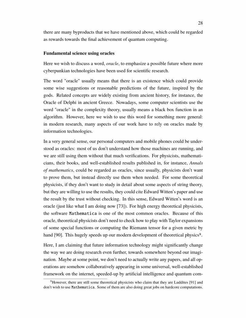
28

there are many byproducts that we have mentioned above, which could be regardedas rewards towards the final achievement of quantum computing.

Fundamental science using oracles

Here we wish to discuss a word, oracle, to emphasize a possible future where morecyberpunkian technologies have been used for scientific research.

The word "oracle" usually means that there is an existence which could providesome wise suggestions or reasonable predictions of the future, inspired by thegods. Related concepts are widely existing from ancient history, for instance, theOracle of Delphi in ancient Greece. Nowadays, some computer scientists use theword "oracle" in the complexity theory, usually means a black box function in analgorithm. However, here we wish to use this word for something more general:in modern research, many aspects of our work have to rely on oracles made byinformation technologies.

In a very general sense, our personal computers and mobile phones could be under-stood as oracles: most of us don’t understand how those machines are running, andwe are still using them without that much verifications. For physicists, mathemati-cians, their books, and well-established results published in, for instance, Annalsof mathematics, could be regarded as oracles, since usually, physicists don’t wantto prove them, but instead directly use them when needed. For some theoreticalphysicists, if they don’t want to study in detail about some aspects of string theory,but they are willing to use the results, they could cite EdwardWitten’s paper and usethe result by the trust without checking. In this sense, Edward Witten’s word is anoracle (just like what I am doing now [73]). For high energy theoretical physicists,the software Mathematica is one of the most common oracles. Because of thisoracle, theoretical physicists don’t need to check how to play with Taylor expansionsof some special functions or computing the Riemann tensor for a given metric byhand [90]. This hugely speeds up our modern development of theoretical physics9.

Here, I am claiming that future information technology might significantly changethe way we are doing research even further, towards somewhere beyond our imagi-nation. Maybe at some point, we don’t need to actually write any papers, and all op-erations are somehow collaboratively appearing in some universal, well-establishedframework on the internet, speeded-up by artificial intelligence and quantum com-

9However, there are still some theoretical physicists who claim that they are Luddites [91] anddon’t wish to use Mathematica. Some of them are also doing great jobs on hardcore computations.

29

puting. Maybe we don’t need to provide any technical details of any works whilemachines will help us figure it out, and humans are just able to provide some genericviews. Anyway, I think some aspects of those stories might happen someday, evenduring my life. These imaginings mean that we need more and more oracles.

Aside from the way we are practically doing science, oracles also often appear inthe scientific contents itself. For instance, the existence of the 3d Ising bootstrapisland for mixed operators is still mysterious. People don’t have enough theoreticalunderstanding of it. The way we obtain it is from complicated crossing equationsand large-scale optimization, which could be regarded as oracles. What is the finalanswer to the critical exponents of the 3d Isingmodel? If we think about this problemin terms of crossing equations, the answer is obtained by the consistency of four-pointcorrelation functions with mixing operators. If we transform it into semidefiniteprogramming, it will be obtained from some super complicated crossing equations.If it turns out that the answer could be represented by some numbers where humanbeings are familiar with, it might be a very deep fact about the transcendental natureof hypergeometric functions, or representation theories about the conformal group.Maybe there is a Ramanujan-type formula hidden there, which might be indicatedby oracles of large-scale optimization, or maybe machine learning [92].

Taking about Ramanujan, I think there are some better examples in mathematicsinstead of physics. In fact, the story of Srinivasa Ramanujan himself is highlyrelated to the original meaning of oracles. During the time Ramanujan lived inthe last century, he did not have a complete education in mathematics, but hecould still discover a large set of amazing formulas about special functions andprime numbers. Many of them were highly intriguing but not proved, inspiringmany potential discoveries from algebraic geometry to number theory10. So howwas he able to find those magic formulas? He said, "An equation for me has nomeaning unless it expresses a thought of God". It seems that he was creditinghis formulas to his family goddess Namagiri Thayar, although some people believethat it was from intuitions behind thinking about math for a long time. Of course,Ramanujan is pretty unique in history, and I am not sure if it is wise enough tochoose some beliefs in order to make some scientific discoveries, but I am sayingthat some future information technology will bring people solid, incomprehensiblepredictions, serving as oracles. In fact, people already start to do this. Thereis a machine learning project made by Google called the Ramanujan Machine,

10If you don’t know his story, you could look at the movie The Man Who Knew Infinity [93].

30

which is trying to discover some conjectural identities about special constants andcontinued fractions [94]. Based on their website [95], they are already able togenerate conjectures by neural networks, and some of them seem not yet proved byprofessional mathematicians.

Besides discovering new conjectures, one of the first steps is probably to try toverify the known proof. About this, I wish to quote some recent activities by a well-established number theorist, Kevin Buzzard (see, for instance, this article [96]).According to him, there is no person on earth who could completely understand alldetails of Fermat’s Last Theorem: the proof is so complicated, and people have touse many known results by trusting the original author, and all those details lead toa huge amount of literature. Nowadays, many aspects of mathematics, for instance,arithmetic algebraic geometry, Langlands program, or closer to physics, symplecticgeometry, become extremely technical, and there is usually a very limited numberof persons who could understand details of the proof. Thus, maybe it is necessary totry to verify some proofs based onmachine, just in the aspects of logical consistency,since unlike modern physics allowing some degrees of fuzzy logic, mathematicalproofs only allow two consequences: correct or wrong.

Kevin Buzzard is working on gathering fundings and establish codes to verifyknown mathematical proofs, and some concepts of new mathematics, for instance,perfectoids introduced by Peter Scholze, could be realized by codes. Maybe thisis a promising direction that is helpful for future mathematics, although youngpeople in this field have to prove themselves by proving theorems. In physics,parts of theoretical physics directions are more rigorous in the mathematical sense,especially some aspects of quantum field theory or quantum information science,since the basic rule is more or less well-established. In other parts, for instance,quantum gravity, people have to make conjectural guess since the building blocksare not completely developed. Maybe for the former, it makes sense to do someverifications also. And in the long-term future, when people really discover a theoryof everything, people could put all physics and mathematics axioms and theoremsin a computer, to make solid predictions in our cyberpunkian future.

The current progress of number theory often tells us how limited people know aboutsome simple concepts like prime numbers or rational numbers. For instance, aboutthe Diophantine equation, the celebrated Birch-Swinnerton-Dyer (BSD) conjecture,one of the Millennium Prize Problems, could tell us something about the structuresof solutions for the cubic equations (not proven). Problems in more general cases,

31

higher degrees, more variables, are extremely hard to answer, while some of themare approaching some deepest sides of modern mathematics, where it is relativelyeasy to formulate a question that no one on the earth could solve. I would feel thatmaybe many of those problems are too hard for human brains, and in the future, wehave to rely on oracles made by cyberpunkian technologies.

Companies, colliders

Here, we wish to comment on the relations between cyberpunkian quantum fieldtheory and phenomenology. In many parts of this article, I am talking aboutsome formal research, which seems to be not that related to real observations andexperiments. However, it is not true. As we mentioned before, strongly-coupledquantum field theories are everywhere: people need to use strongly-coupled QCD topredict meson spectra and real-time dynamics happening in some colliders. In thecondensed-matter system and statistical physics, predictions from strongly-coupledfield theory are helpful to study strong-correlated systems, and they are directlymeasurable as quantum materials. In the sky, models with dark matter and darkenergy might need strongly-coupled field theories to understand, cosmic phasetransitions happening in the early universe might also be an exotic strongly-coupledfield theory phenomena. Black hole physics is directly related to observationsfrom event horizon telescope and LIGO (Laser Interferometer Gravitational-WaveObservatory) experiments about gravitational waves. I feel that all of them mightneed potential computational speedup or formal understanding from informationtheory. In a sense, they are all cyberpunkian physics!

It might be interesting to comment on some modern aspects of relations betweenacademia and industry. Traditionally, some people studying fundamental physicsmight feel that pure potential physical breakthroughs may not be related to anycommercial companies. However, I feel that in our quantum era, it might becommon that academia and industry will have more communications.

Many companies, for instance, Google, Amazon, Microsoft, IBM, etc., have theambition nowadays to make useful quantum computers for potential commercialpurposes. Scientific academia, as part of public service sometimes funded by thegovernment and donation, is aiming at providing high-quality research about ournature. In our quantum era, people start to communicate with each side frequently.We often see examples where quantum information scientists switch back and forthbetween two sides, and make great progress for both. There are several quantum

32

number of qubits<latexit sha1_base64="QSFHOKk6fdrgOu0ZVXZpAxD4pow=">AAAC3HicjVHLSsNAFD2Nr1pfVRcu3ASL4KqkIuiy6MZlBfuAtpYkndaheTmZiKV0507c+gNu9XvEP9C/8M6YglpEJyQ5c+49Z+6d60Qej6VlvWaMmdm5+YXsYm5peWV1Lb++UYvDRLis6oZeKBqOHTOPB6wqufRYIxLM9h2P1Z3BiYrXr5mIeRicy2HE2r7dD3iPu7YkqpPfakl2I0dB4jtMmGHPvEocLuNxJ1+wipZe5jQopaCAdFXC/Ata6CKEiwQ+GAJIwh5sxPQ0UYKFiLg2RsQJQlzHGcbIkTahLEYZNrED+vZp10zZgPbKM9Zql07x6BWkNLFLmpDyBGF1mqnjiXZW7G/eI+2pahvS30m9fGIlLon9SzfJ/K9O9SLRw5HugVNPkWZUd27qkuhbUZWbX7qS5BARp3CX4oKwq5WTeza1Jta9q7u1dfxNZypW7d00N8G7qpIGXPo5zmlQ2y+WCJ8dFMrH6aiz2MYO9miehyjjFBVUdf2PeMKzcWHcGnfG/WeqkUk1m/i2jIcPpfCZYQ==</latexit><latexit sha1_base64="QSFHOKk6fdrgOu0ZVXZpAxD4pow=">AAAC3HicjVHLSsNAFD2Nr1pfVRcu3ASL4KqkIuiy6MZlBfuAtpYkndaheTmZiKV0507c+gNu9XvEP9C/8M6YglpEJyQ5c+49Z+6d60Qej6VlvWaMmdm5+YXsYm5peWV1Lb++UYvDRLis6oZeKBqOHTOPB6wqufRYIxLM9h2P1Z3BiYrXr5mIeRicy2HE2r7dD3iPu7YkqpPfakl2I0dB4jtMmGHPvEocLuNxJ1+wipZe5jQopaCAdFXC/Ata6CKEiwQ+GAJIwh5sxPQ0UYKFiLg2RsQJQlzHGcbIkTahLEYZNrED+vZp10zZgPbKM9Zql07x6BWkNLFLmpDyBGF1mqnjiXZW7G/eI+2pahvS30m9fGIlLon9SzfJ/K9O9SLRw5HugVNPkWZUd27qkuhbUZWbX7qS5BARp3CX4oKwq5WTeza1Jta9q7u1dfxNZypW7d00N8G7qpIGXPo5zmlQ2y+WCJ8dFMrH6aiz2MYO9miehyjjFBVUdf2PeMKzcWHcGnfG/WeqkUk1m/i2jIcPpfCZYQ==</latexit><latexit sha1_base64="QSFHOKk6fdrgOu0ZVXZpAxD4pow=">AAAC3HicjVHLSsNAFD2Nr1pfVRcu3ASL4KqkIuiy6MZlBfuAtpYkndaheTmZiKV0507c+gNu9XvEP9C/8M6YglpEJyQ5c+49Z+6d60Qej6VlvWaMmdm5+YXsYm5peWV1Lb++UYvDRLis6oZeKBqOHTOPB6wqufRYIxLM9h2P1Z3BiYrXr5mIeRicy2HE2r7dD3iPu7YkqpPfakl2I0dB4jtMmGHPvEocLuNxJ1+wipZe5jQopaCAdFXC/Ata6CKEiwQ+GAJIwh5sxPQ0UYKFiLg2RsQJQlzHGcbIkTahLEYZNrED+vZp10zZgPbKM9Zql07x6BWkNLFLmpDyBGF1mqnjiXZW7G/eI+2pahvS30m9fGIlLon9SzfJ/K9O9SLRw5HugVNPkWZUd27qkuhbUZWbX7qS5BARp3CX4oKwq5WTeza1Jta9q7u1dfxNZypW7d00N8G7qpIGXPo5zmlQ2y+WCJ8dFMrH6aiz2MYO9miehyjjFBVUdf2PeMKzcWHcGnfG/WeqkUk1m/i2jIcPpfCZYQ==</latexit><latexit sha1_base64="QSFHOKk6fdrgOu0ZVXZpAxD4pow=">AAAC3HicjVHLSsNAFD2Nr1pfVRcu3ASL4KqkIuiy6MZlBfuAtpYkndaheTmZiKV0507c+gNu9XvEP9C/8M6YglpEJyQ5c+49Z+6d60Qej6VlvWaMmdm5+YXsYm5peWV1Lb++UYvDRLis6oZeKBqOHTOPB6wqufRYIxLM9h2P1Z3BiYrXr5mIeRicy2HE2r7dD3iPu7YkqpPfakl2I0dB4jtMmGHPvEocLuNxJ1+wipZe5jQopaCAdFXC/Ata6CKEiwQ+GAJIwh5sxPQ0UYKFiLg2RsQJQlzHGcbIkTahLEYZNrED+vZp10zZgPbKM9Zql07x6BWkNLFLmpDyBGF1mqnjiXZW7G/eI+2pahvS30m9fGIlLon9SzfJ/K9O9SLRw5HugVNPkWZUd27qkuhbUZWbX7qS5BARp3CX4oKwq5WTeza1Jta9q7u1dfxNZypW7d00N8G7qpIGXPo5zmlQ2y+WCJ8dFMrH6aiz2MYO9miehyjjFBVUdf2PeMKzcWHcGnfG/WeqkUk1m/i2jIcPpfCZYQ==</latexit>

number of T-gates<latexit sha1_base64="WHsjhy2RogsR51YLdlilpyo9m9Y=">AAAC3XicjVHLSsNAFD2Nr1pfUTeCm2AR3FgSEXRZdOOyQl/QSknSaQ3Ni8lELKXu3Ilbf8Ct/o74B/oX3hlTUIvohCRnzr3nzNx7ndj3EmGarzltZnZufiG/WFhaXlld09c36kmUcpfV3MiPeNOxE+Z7IasJT/isGXNmB47PGs7gVMYbV4wnXhRWxTBmF4HdD72e59qCqI6+1RbsWozCNHAYN6KeUd3v24Il445eNEumWsY0sDJQRLYqkf6CNrqI4CJFAIYQgrAPGwk9LVgwERN3gRFxnJCn4gxjFEibUhajDJvYAX37tGtlbEh76ZkotUun+PRyUhrYJU1EeZywPM1Q8VQ5S/Y375HylHcb0t/JvAJiBS6J/Us3yfyvTtYi0MOxqsGjmmLFyOrczCVVXZE3N75UJcghJk7iLsU5YVcpJ302lCZRtcve2ir+pjIlK/dulpviXd6SBmz9HOc0qB+ULMLnh8XySTbqPLaxgz2a5xHKOEMFNfK+wSOe8Kx1tFvtTrv/TNVymWYT35b28AHLgplo</latexit><latexit sha1_base64="WHsjhy2RogsR51YLdlilpyo9m9Y=">AAAC3XicjVHLSsNAFD2Nr1pfUTeCm2AR3FgSEXRZdOOyQl/QSknSaQ3Ni8lELKXu3Ilbf8Ct/o74B/oX3hlTUIvohCRnzr3nzNx7ndj3EmGarzltZnZufiG/WFhaXlld09c36kmUcpfV3MiPeNOxE+Z7IasJT/isGXNmB47PGs7gVMYbV4wnXhRWxTBmF4HdD72e59qCqI6+1RbsWozCNHAYN6KeUd3v24Il445eNEumWsY0sDJQRLYqkf6CNrqI4CJFAIYQgrAPGwk9LVgwERN3gRFxnJCn4gxjFEibUhajDJvYAX37tGtlbEh76ZkotUun+PRyUhrYJU1EeZywPM1Q8VQ5S/Y375HylHcb0t/JvAJiBS6J/Us3yfyvTtYi0MOxqsGjmmLFyOrczCVVXZE3N75UJcghJk7iLsU5YVcpJ302lCZRtcve2ir+pjIlK/dulpviXd6SBmz9HOc0qB+ULMLnh8XySTbqPLaxgz2a5xHKOEMFNfK+wSOe8Kx1tFvtTrv/TNVymWYT35b28AHLgplo</latexit><latexit sha1_base64="WHsjhy2RogsR51YLdlilpyo9m9Y=">AAAC3XicjVHLSsNAFD2Nr1pfUTeCm2AR3FgSEXRZdOOyQl/QSknSaQ3Ni8lELKXu3Ilbf8Ct/o74B/oX3hlTUIvohCRnzr3nzNx7ndj3EmGarzltZnZufiG/WFhaXlld09c36kmUcpfV3MiPeNOxE+Z7IasJT/isGXNmB47PGs7gVMYbV4wnXhRWxTBmF4HdD72e59qCqI6+1RbsWozCNHAYN6KeUd3v24Il445eNEumWsY0sDJQRLYqkf6CNrqI4CJFAIYQgrAPGwk9LVgwERN3gRFxnJCn4gxjFEibUhajDJvYAX37tGtlbEh76ZkotUun+PRyUhrYJU1EeZywPM1Q8VQ5S/Y375HylHcb0t/JvAJiBS6J/Us3yfyvTtYi0MOxqsGjmmLFyOrczCVVXZE3N75UJcghJk7iLsU5YVcpJ302lCZRtcve2ir+pjIlK/dulpviXd6SBmz9HOc0qB+ULMLnh8XySTbqPLaxgz2a5xHKOEMFNfK+wSOe8Kx1tFvtTrv/TNVymWYT35b28AHLgplo</latexit><latexit sha1_base64="WHsjhy2RogsR51YLdlilpyo9m9Y=">AAAC3XicjVHLSsNAFD2Nr1pfUTeCm2AR3FgSEXRZdOOyQl/QSknSaQ3Ni8lELKXu3Ilbf8Ct/o74B/oX3hlTUIvohCRnzr3nzNx7ndj3EmGarzltZnZufiG/WFhaXlld09c36kmUcpfV3MiPeNOxE+Z7IasJT/isGXNmB47PGs7gVMYbV4wnXhRWxTBmF4HdD72e59qCqI6+1RbsWozCNHAYN6KeUd3v24Il445eNEumWsY0sDJQRLYqkf6CNrqI4CJFAIYQgrAPGwk9LVgwERN3gRFxnJCn4gxjFEibUhajDJvYAX37tGtlbEh76ZkotUun+PRyUhrYJU1EeZywPM1Q8VQ5S/Y375HylHcb0t/JvAJiBS6J/Us3yfyvTtYi0MOxqsGjmmLFyOrczCVVXZE3N75UJcghJk7iLsU5YVcpJ302lCZRtcve2ir+pjIlK/dulpviXd6SBmz9HOc0qB+ULMLnh8XySTbqPLaxgz2a5xHKOEMFNfK+wSOe8Kx1tFvtTrv/TNVymWYT35b28AHLgplo</latexit>

Google device<latexit sha1_base64="GgKrvdGuVtCSG0qJushu2a8O74w=">AAAC2XicjVHLSsNAFD2N7/qqj52bYBFcSSqCLkUXulSwWmilJNOxDk4zYTIRa+nCnbj1B9zqD4l/oH/hnTEFH4hOSHLm3HvOzL03SqRITRC8FLyh4ZHRsfGJ4uTU9MxsaW7+OFWZZrzKlFS6FoUplyLmVSOM5LVE87ATSX4SXeza+Mkl16lQ8ZHpJvy0E7ZjcSZYaIhqlhYbhl+Z3p5Sbcn9Fr8UjPebpXKwFrjl/wSVHJSRrwNVekYDLSgwZOiAI4YhLBEipaeOCgIkxJ2iR5wmJFyco48iaTPK4pQREntB3zbt6jkb0956pk7N6BRJryaljxXSKMrThO1pvotnztmyv3n3nKe9W5f+Ue7VIdbgnNi/dIPM/+psLQZn2HI1CKopcYytjuUumeuKvbn/qSpDDglxFrcorgkzpxz02Xea1NVuexu6+KvLtKzdszw3w5u9JQ248n2cP8Hx+lqF8OFGeXsnH/U4lrCMVZrnJraxjwNUyfsaD3jEk1f3brxb7+4j1SvkmgV8Wd79Owvml/o=</latexit><latexit sha1_base64="GgKrvdGuVtCSG0qJushu2a8O74w=">AAAC2XicjVHLSsNAFD2N7/qqj52bYBFcSSqCLkUXulSwWmilJNOxDk4zYTIRa+nCnbj1B9zqD4l/oH/hnTEFH4hOSHLm3HvOzL03SqRITRC8FLyh4ZHRsfGJ4uTU9MxsaW7+OFWZZrzKlFS6FoUplyLmVSOM5LVE87ATSX4SXeza+Mkl16lQ8ZHpJvy0E7ZjcSZYaIhqlhYbhl+Z3p5Sbcn9Fr8UjPebpXKwFrjl/wSVHJSRrwNVekYDLSgwZOiAI4YhLBEipaeOCgIkxJ2iR5wmJFyco48iaTPK4pQREntB3zbt6jkb0956pk7N6BRJryaljxXSKMrThO1pvotnztmyv3n3nKe9W5f+Ue7VIdbgnNi/dIPM/+psLQZn2HI1CKopcYytjuUumeuKvbn/qSpDDglxFrcorgkzpxz02Xea1NVuexu6+KvLtKzdszw3w5u9JQ248n2cP8Hx+lqF8OFGeXsnH/U4lrCMVZrnJraxjwNUyfsaD3jEk1f3brxb7+4j1SvkmgV8Wd79Owvml/o=</latexit><latexit sha1_base64="GgKrvdGuVtCSG0qJushu2a8O74w=">AAAC2XicjVHLSsNAFD2N7/qqj52bYBFcSSqCLkUXulSwWmilJNOxDk4zYTIRa+nCnbj1B9zqD4l/oH/hnTEFH4hOSHLm3HvOzL03SqRITRC8FLyh4ZHRsfGJ4uTU9MxsaW7+OFWZZrzKlFS6FoUplyLmVSOM5LVE87ATSX4SXeza+Mkl16lQ8ZHpJvy0E7ZjcSZYaIhqlhYbhl+Z3p5Sbcn9Fr8UjPebpXKwFrjl/wSVHJSRrwNVekYDLSgwZOiAI4YhLBEipaeOCgIkxJ2iR5wmJFyco48iaTPK4pQREntB3zbt6jkb0956pk7N6BRJryaljxXSKMrThO1pvotnztmyv3n3nKe9W5f+Ue7VIdbgnNi/dIPM/+psLQZn2HI1CKopcYytjuUumeuKvbn/qSpDDglxFrcorgkzpxz02Xea1NVuexu6+KvLtKzdszw3w5u9JQ248n2cP8Hx+lqF8OFGeXsnH/U4lrCMVZrnJraxjwNUyfsaD3jEk1f3brxb7+4j1SvkmgV8Wd79Owvml/o=</latexit><latexit sha1_base64="GgKrvdGuVtCSG0qJushu2a8O74w=">AAAC2XicjVHLSsNAFD2N7/qqj52bYBFcSSqCLkUXulSwWmilJNOxDk4zYTIRa+nCnbj1B9zqD4l/oH/hnTEFH4hOSHLm3HvOzL03SqRITRC8FLyh4ZHRsfGJ4uTU9MxsaW7+OFWZZrzKlFS6FoUplyLmVSOM5LVE87ATSX4SXeza+Mkl16lQ8ZHpJvy0E7ZjcSZYaIhqlhYbhl+Z3p5Sbcn9Fr8UjPebpXKwFrjl/wSVHJSRrwNVekYDLSgwZOiAI4YhLBEipaeOCgIkxJ2iR5wmJFyco48iaTPK4pQREntB3zbt6jkb0956pk7N6BRJryaljxXSKMrThO1pvotnztmyv3n3nKe9W5f+Ue7VIdbgnNi/dIPM/+psLQZn2HI1CKopcYytjuUumeuKvbn/qSpDDglxFrcorgkzpxz02Xea1NVuexu6+KvLtKzdszw3w5u9JQ248n2cP8Hx+lqF8OFGeXsnH/U4lrCMVZrnJraxjwNUyfsaD3jEk1f3brxb7+4j1SvkmgV8Wd79Owvml/o=</latexit>

IBM device<latexit sha1_base64="dqk8BAlIHmJ/w1UiiV8eqBJ61HU=">AAAC1nicjVHLSsNAFD2Nr1pfrS7dBIvgqqQi6LLUjS6ECvYBbZFkOq1D0yQkk2opdSdu/QG3+kniH+hfeGdMQS2iE5KcOfeeM3PvdQJXRNKyXlPG3PzC4lJ6ObOyura+kc1t1iI/DhmvMt/1w4ZjR9wVHq9KIV3eCEJuDxyX153+sYrXhzyMhO9dyFHA2wO754muYLYk6jKba0l+I8en5TOzw4eC8cllNm8VLL3MWVBMQB7JqvjZF7TQgQ+GGANweJCEXdiI6GmiCAsBcW2MiQsJCR3nmCBD2piyOGXYxPbp26NdM2E92ivPSKsZneLSG5LSxC5pfMoLCavTTB2PtbNif/Mea091txH9ncRrQKzEFbF/6aaZ/9WpWiS6ONI1CKop0IyqjiUuse6Kurn5pSpJDgFxCncoHhJmWjnts6k1ka5d9dbW8TedqVi1Z0lujHd1Sxpw8ec4Z0Ftv1AkfH6QL5WTUaexjR3s0TwPUcIJKqiS9zUe8YRno2HcGnfG/WeqkUo0W/i2jIcP5OqWVw==</latexit><latexit sha1_base64="dqk8BAlIHmJ/w1UiiV8eqBJ61HU=">AAAC1nicjVHLSsNAFD2Nr1pfrS7dBIvgqqQi6LLUjS6ECvYBbZFkOq1D0yQkk2opdSdu/QG3+kniH+hfeGdMQS2iE5KcOfeeM3PvdQJXRNKyXlPG3PzC4lJ6ObOyura+kc1t1iI/DhmvMt/1w4ZjR9wVHq9KIV3eCEJuDxyX153+sYrXhzyMhO9dyFHA2wO754muYLYk6jKba0l+I8en5TOzw4eC8cllNm8VLL3MWVBMQB7JqvjZF7TQgQ+GGANweJCEXdiI6GmiCAsBcW2MiQsJCR3nmCBD2piyOGXYxPbp26NdM2E92ivPSKsZneLSG5LSxC5pfMoLCavTTB2PtbNif/Mea091txH9ncRrQKzEFbF/6aaZ/9WpWiS6ONI1CKop0IyqjiUuse6Kurn5pSpJDgFxCncoHhJmWjnts6k1ka5d9dbW8TedqVi1Z0lujHd1Sxpw8ec4Z0Ftv1AkfH6QL5WTUaexjR3s0TwPUcIJKqiS9zUe8YRno2HcGnfG/WeqkUo0W/i2jIcP5OqWVw==</latexit><latexit sha1_base64="dqk8BAlIHmJ/w1UiiV8eqBJ61HU=">AAAC1nicjVHLSsNAFD2Nr1pfrS7dBIvgqqQi6LLUjS6ECvYBbZFkOq1D0yQkk2opdSdu/QG3+kniH+hfeGdMQS2iE5KcOfeeM3PvdQJXRNKyXlPG3PzC4lJ6ObOyura+kc1t1iI/DhmvMt/1w4ZjR9wVHq9KIV3eCEJuDxyX153+sYrXhzyMhO9dyFHA2wO754muYLYk6jKba0l+I8en5TOzw4eC8cllNm8VLL3MWVBMQB7JqvjZF7TQgQ+GGANweJCEXdiI6GmiCAsBcW2MiQsJCR3nmCBD2piyOGXYxPbp26NdM2E92ivPSKsZneLSG5LSxC5pfMoLCavTTB2PtbNif/Mea091txH9ncRrQKzEFbF/6aaZ/9WpWiS6ONI1CKop0IyqjiUuse6Kurn5pSpJDgFxCncoHhJmWjnts6k1ka5d9dbW8TedqVi1Z0lujHd1Sxpw8ec4Z0Ftv1AkfH6QL5WTUaexjR3s0TwPUcIJKqiS9zUe8YRno2HcGnfG/WeqkUo0W/i2jIcP5OqWVw==</latexit><latexit sha1_base64="dqk8BAlIHmJ/w1UiiV8eqBJ61HU=">AAAC1nicjVHLSsNAFD2Nr1pfrS7dBIvgqqQi6LLUjS6ECvYBbZFkOq1D0yQkk2opdSdu/QG3+kniH+hfeGdMQS2iE5KcOfeeM3PvdQJXRNKyXlPG3PzC4lJ6ObOyura+kc1t1iI/DhmvMt/1w4ZjR9wVHq9KIV3eCEJuDxyX153+sYrXhzyMhO9dyFHA2wO754muYLYk6jKba0l+I8en5TOzw4eC8cllNm8VLL3MWVBMQB7JqvjZF7TQgQ+GGANweJCEXdiI6GmiCAsBcW2MiQsJCR3nmCBD2piyOGXYxPbp26NdM2E92ivPSKsZneLSG5LSxC5pfMoLCavTTB2PtbNif/Mea091txH9ncRrQKzEFbF/6aaZ/9WpWiS6ONI1CKop0IyqjiUuse6Kurn5pSpJDgFxCncoHhJmWjnts6k1ka5d9dbW8TedqVi1Z0lujHd1Sxpw8ec4Z0Ftv1AkfH6QL5WTUaexjR3s0TwPUcIJKqiS9zUe8YRno2HcGnfG/WeqkUo0W/i2jIcP5OqWVw==</latexit>

Predicting physics @ LHC<latexit sha1_base64="e4UC7Lr3TBCe9z656D4rzOsOEKA=">AAAC5HicjVHLSsNAFD3GV31XXbowWARXkoqgy6IbFy4q2FaopSTTaR1MkzAzEUvp0p07cesPuNVvEf9A/8I7YwpqEZ2Q5My595yZe2+QhEJpz3sdc8YnJqemczOzc/MLi0v55ZWqilPJeIXFYSzPAl/xUES8ooUO+Vkiud8NQl4LLg9NvHbFpRJxdKp7CW90/U4k2oL5mqhmfv1c82vdL0veEkyLqOMmFz0lmHJL7vHR4aCZL3jbnl3uKChmoIBsleP8C87RQgyGFF1wRNCEQ/hQ9NRRhIeEuAb6xElCwsY5BpglbUpZnDJ8Yi/p26FdPWMj2htPZdWMTgnplaR0sUmamPIkYXOaa+OpdTbsb95962nu1qN/kHl1idW4IPYv3TDzvzpTi0Yb+7YGQTUlljHVscwltV0xN3e/VKXJISHO4BbFJWFmlcM+u1ajbO2mt76Nv9lMw5o9y3JTvJtb0oCLP8c5Cqo720XCJ7uF0kE26hzWsIEtmuceSjhCGRXyvsEjnvDstJ1b5865/0x1xjLNKr4t5+EDoHWb/g==</latexit><latexit sha1_base64="e4UC7Lr3TBCe9z656D4rzOsOEKA=">AAAC5HicjVHLSsNAFD3GV31XXbowWARXkoqgy6IbFy4q2FaopSTTaR1MkzAzEUvp0p07cesPuNVvEf9A/8I7YwpqEZ2Q5My595yZe2+QhEJpz3sdc8YnJqemczOzc/MLi0v55ZWqilPJeIXFYSzPAl/xUES8ooUO+Vkiud8NQl4LLg9NvHbFpRJxdKp7CW90/U4k2oL5mqhmfv1c82vdL0veEkyLqOMmFz0lmHJL7vHR4aCZL3jbnl3uKChmoIBsleP8C87RQgyGFF1wRNCEQ/hQ9NRRhIeEuAb6xElCwsY5BpglbUpZnDJ8Yi/p26FdPWMj2htPZdWMTgnplaR0sUmamPIkYXOaa+OpdTbsb95962nu1qN/kHl1idW4IPYv3TDzvzpTi0Yb+7YGQTUlljHVscwltV0xN3e/VKXJISHO4BbFJWFmlcM+u1ajbO2mt76Nv9lMw5o9y3JTvJtb0oCLP8c5Cqo720XCJ7uF0kE26hzWsIEtmuceSjhCGRXyvsEjnvDstJ1b5865/0x1xjLNKr4t5+EDoHWb/g==</latexit><latexit sha1_base64="e4UC7Lr3TBCe9z656D4rzOsOEKA=">AAAC5HicjVHLSsNAFD3GV31XXbowWARXkoqgy6IbFy4q2FaopSTTaR1MkzAzEUvp0p07cesPuNVvEf9A/8I7YwpqEZ2Q5My595yZe2+QhEJpz3sdc8YnJqemczOzc/MLi0v55ZWqilPJeIXFYSzPAl/xUES8ooUO+Vkiud8NQl4LLg9NvHbFpRJxdKp7CW90/U4k2oL5mqhmfv1c82vdL0veEkyLqOMmFz0lmHJL7vHR4aCZL3jbnl3uKChmoIBsleP8C87RQgyGFF1wRNCEQ/hQ9NRRhIeEuAb6xElCwsY5BpglbUpZnDJ8Yi/p26FdPWMj2htPZdWMTgnplaR0sUmamPIkYXOaa+OpdTbsb95962nu1qN/kHl1idW4IPYv3TDzvzpTi0Yb+7YGQTUlljHVscwltV0xN3e/VKXJISHO4BbFJWFmlcM+u1ajbO2mt76Nv9lMw5o9y3JTvJtb0oCLP8c5Cqo720XCJ7uF0kE26hzWsIEtmuceSjhCGRXyvsEjnvDstJ1b5865/0x1xjLNKr4t5+EDoHWb/g==</latexit><latexit sha1_base64="e4UC7Lr3TBCe9z656D4rzOsOEKA=">AAAC5HicjVHLSsNAFD3GV31XXbowWARXkoqgy6IbFy4q2FaopSTTaR1MkzAzEUvp0p07cesPuNVvEf9A/8I7YwpqEZ2Q5My595yZe2+QhEJpz3sdc8YnJqemczOzc/MLi0v55ZWqilPJeIXFYSzPAl/xUES8ooUO+Vkiud8NQl4LLg9NvHbFpRJxdKp7CW90/U4k2oL5mqhmfv1c82vdL0veEkyLqOMmFz0lmHJL7vHR4aCZL3jbnl3uKChmoIBsleP8C87RQgyGFF1wRNCEQ/hQ9NRRhIeEuAb6xElCwsY5BpglbUpZnDJ8Yi/p26FdPWMj2htPZdWMTgnplaR0sUmamPIkYXOaa+OpdTbsb95962nu1qN/kHl1idW4IPYv3TDzvzpTi0Yb+7YGQTUlljHVscwltV0xN3e/VKXJISHO4BbFJWFmlcM+u1ajbO2mt76Nv9lMw5o9y3JTvJtb0oCLP8c5Cqo720XCJ7uF0kE26hzWsIEtmuceSjhCGRXyvsEjnvDstJ1b5865/0x1xjLNKr4t5+EDoHWb/g==</latexit>

Predicting physics @ LIGO<latexit sha1_base64="c2EPSEztAMx3imoec3UgGeCYoNw=">AAAC5XicjVHLSsNAFD2N73fVpZvBIriSVARdFl2oIFjB1oKKJNOxDqZJmJmIpbh1507c+gNu9VfEP9C/8M4YQS2iE5KcOfeeM3PvDdNIauP7LwWvr39gcGh4ZHRsfGJyqjg9U9dJprio8SRKVCMMtIhkLGpGmkg0UiWCdhiJg/B8w8YPLoTSMon3TScVx+2gFctTyQND1EmRHRlxabpVJZqSGxm3WHrW0ZJrVmE725u7VyfFkr/ku8V6QTkHJeSrmhSfcYQmEnBkaEMghiEcIYCm5xBl+EiJO0aXOEVIurjAFUZJm1GWoIyA2HP6tmh3mLMx7a2ndmpOp0T0KlIyLJAmoTxF2J7GXDxzzpb9zbvrPO3dOvQPc682sQZnxP6l+8z8r87WYnCKNVeDpJpSx9jqeO6Sua7Ym7MvVRlySImzuElxRZg75WefmdNoV7vtbeDiry7TsnbP89wMb/aWNODyz3H2gvryUpnw3kqpsp6PehhzmMcizXMVFWyhihp5X+MBj3jyWt6Nd+vdfaR6hVwzi2/Lu38HmZicXA==</latexit><latexit sha1_base64="c2EPSEztAMx3imoec3UgGeCYoNw=">AAAC5XicjVHLSsNAFD2N73fVpZvBIriSVARdFl2oIFjB1oKKJNOxDqZJmJmIpbh1507c+gNu9VfEP9C/8M4YQS2iE5KcOfeeM3PvDdNIauP7LwWvr39gcGh4ZHRsfGJyqjg9U9dJprio8SRKVCMMtIhkLGpGmkg0UiWCdhiJg/B8w8YPLoTSMon3TScVx+2gFctTyQND1EmRHRlxabpVJZqSGxm3WHrW0ZJrVmE725u7VyfFkr/ku8V6QTkHJeSrmhSfcYQmEnBkaEMghiEcIYCm5xBl+EiJO0aXOEVIurjAFUZJm1GWoIyA2HP6tmh3mLMx7a2ndmpOp0T0KlIyLJAmoTxF2J7GXDxzzpb9zbvrPO3dOvQPc682sQZnxP6l+8z8r87WYnCKNVeDpJpSx9jqeO6Sua7Ym7MvVRlySImzuElxRZg75WefmdNoV7vtbeDiry7TsnbP89wMb/aWNODyz3H2gvryUpnw3kqpsp6PehhzmMcizXMVFWyhihp5X+MBj3jyWt6Nd+vdfaR6hVwzi2/Lu38HmZicXA==</latexit><latexit sha1_base64="c2EPSEztAMx3imoec3UgGeCYoNw=">AAAC5XicjVHLSsNAFD2N73fVpZvBIriSVARdFl2oIFjB1oKKJNOxDqZJmJmIpbh1507c+gNu9VfEP9C/8M4YQS2iE5KcOfeeM3PvDdNIauP7LwWvr39gcGh4ZHRsfGJyqjg9U9dJprio8SRKVCMMtIhkLGpGmkg0UiWCdhiJg/B8w8YPLoTSMon3TScVx+2gFctTyQND1EmRHRlxabpVJZqSGxm3WHrW0ZJrVmE725u7VyfFkr/ku8V6QTkHJeSrmhSfcYQmEnBkaEMghiEcIYCm5xBl+EiJO0aXOEVIurjAFUZJm1GWoIyA2HP6tmh3mLMx7a2ndmpOp0T0KlIyLJAmoTxF2J7GXDxzzpb9zbvrPO3dOvQPc682sQZnxP6l+8z8r87WYnCKNVeDpJpSx9jqeO6Sua7Ym7MvVRlySImzuElxRZg75WefmdNoV7vtbeDiry7TsnbP89wMb/aWNODyz3H2gvryUpnw3kqpsp6PehhzmMcizXMVFWyhihp5X+MBj3jyWt6Nd+vdfaR6hVwzi2/Lu38HmZicXA==</latexit><latexit sha1_base64="c2EPSEztAMx3imoec3UgGeCYoNw=">AAAC5XicjVHLSsNAFD2N73fVpZvBIriSVARdFl2oIFjB1oKKJNOxDqZJmJmIpbh1507c+gNu9VfEP9C/8M4YQS2iE5KcOfeeM3PvDdNIauP7LwWvr39gcGh4ZHRsfGJyqjg9U9dJprio8SRKVCMMtIhkLGpGmkg0UiWCdhiJg/B8w8YPLoTSMon3TScVx+2gFctTyQND1EmRHRlxabpVJZqSGxm3WHrW0ZJrVmE725u7VyfFkr/ku8V6QTkHJeSrmhSfcYQmEnBkaEMghiEcIYCm5xBl+EiJO0aXOEVIurjAFUZJm1GWoIyA2HP6tmh3mLMx7a2ndmpOp0T0KlIyLJAmoTxF2J7GXDxzzpb9zbvrPO3dOvQPc682sQZnxP6l+8z8r87WYnCKNVeDpJpSx9jqeO6Sua7Ym7MvVRlySImzuElxRZg75WefmdNoV7vtbeDiry7TsnbP89wMb/aWNODyz3H2gvryUpnw3kqpsp6PehhzmMcizXMVFWyhihp5X+MBj3jyWt6Nd+vdfaR6hVwzi2/Lu38HmZicXA==</latexit>

Figure 1.5: An imaginary plot might be made by future cyberpunkian physi-cists, especially high energy phenomenologists. This kind of plot includes therequired computational resource needed for observations and existing computa-tional resources provided by companies. As far as I know, no such plot existed untilJune 2021, which put together experimental organizations and quantum companies.I am conjecturing here that this type of plot will appear in the future.

centers from commercial companies established around the university campus, forinstance, Microsoft Station Q at Santa Barbara, and the new Amazon quantumcenter at Pasadena. One remarkable work done recently about simulating quantumgravity in the lab is also such a great collaboration between company and university[84]. For me, it is exciting to imagine that Google is starting to probe properties oftraversable wormholes.

It is exciting to see that both government and private industrial communities arewilling to help establish some exciting new areas relating to fundamental physics andinformation technology. Previously, I am impressed by some high energy physicsresearch collecting data from completely different experimental organizations andcomparing them with each other. For instance, the electroweak phase transitionhappening in the early universe, might need observational and experimental databoth from the ground (colliders) and the sky (gravitational wave detectors), and thedata analysis might be made in the same plot (see, for instance, Figure 2 of [97]). Iam imagining that one day, people will make plots which mention companies likeGoogle and IBM, experimental organizations like LHC and LIGO in the same place(See Figure 1.5). I hope that the day may not be too far off.

33

C h a p t e r 2

PROOF OF THE WEAK GRAVITY CONJECTURE FROMBLACK HOLE ENTROPY

This chapter is based on C. Cheung, J. Liu and G. N. Remmen, Proof of theWeak Gravity Conjecture from Black Hole Entropy, JHEP 1810, 004 (2018),arXiv:1801.08546 [hep-th].

Abstract: We prove that higher-dimension operators contribute positively to theentropy of a thermodynamically stable black hole at fixed mass and charge. Ourresults apply whenever the dominant corrections originate at tree level from quan-tum field theoretic dynamics. More generally, positivity of the entropy shift isequivalent to a certain inequality relating the free energies of black holes. Theseentropy inequalities mandate new positivity bounds on the coefficients of higher-dimension operators. One of these conditions implies that the charge- to-massratio of an extremal black hole asymptotes to unity from above for increasing mass.Consequently, large extremal black holes are unstable to decay to smaller extremalblack holes and the weak gravity conjecture is automatically satisfied. Our findingsgeneralize to arbitrary spacetime dimension and to the case of multiple gauge fields.The assumptions of this proof are valid across a range of scenarios, including stringtheory constructions with a dilaton stabilized below the string scale.

2.1 IntroductionIn this paper we argue that black hole thermodynamics implies new constraints onthe coefficients of higher-dimension operators. Our results are based on a certainuniversal property of entropy. In particular, consider a system T prepared in amacrostate whose microstate degeneracy is quantified by entropy S. Now let usdefine the system T to be a restriction of T in which a handful of degrees offreedom have been frozen to a fixed configuration. If T is prepared in the samemacrostate as T , then the corresponding entropy S will be less than S because themicrostate degeneracy is diminished. Thus, we find that

S = S + ∆S, (2.1)

where the entropy shift ∆S is strictly positive.

34

A similar logic applies to black hole entropy. Consider the low-energy effectivefield theory of photons and gravitons in general spacetime dimension D, defined ata scale far below the mass gap. The effective Lagrangian is

L = L + ∆L, (2.2)

where the first term describes pure Einstein-Maxwell theory,1

L =1

2κ2 R −14

FµνFµν, (2.3)

and the second term encodes corrections from higher-dimension operators,

∆L = c1R2 + c2RµνRµν + c3RµνρσRµνρσ

+ c4RFµνFµν + c5RµνFµρFνρ + c6RµνρσFµνFρσ

+ c7FµνFµνFρσFρσ + c8FµνFνρFρσFσµ.

(2.4)

Without loss of generality, we have dropped all terms involving ∇ρFµν, whichare equivalent via the Bianchi identities to terms already accounted for or termsinvolving ∇µFµν [98], which vanish in the absence of charged matter sources,which we assume throughout.

For our analysis, we study a large black hole of fixed mass m and charge q asmeasured in natural units at spatial infinity. In the presence of higher-dimensionoperators, the metric is

gµν = gµν + ∆gµν . (2.5)

Unless otherwise stated, all variables with tildes like gµν will denote quantitiescorresponding to a Reissner-Nordström black hole of the same mass and chargein pure Einstein-Maxwell theory, while variables with deltas like ∆gµν will denotethe leading corrections from higher-dimension operators, which are linear in thecoefficients ci.

It is straightforward to compute the black hole entropy using theWald formula [99],2

S = −2π∫Σ

δL

δRµνρσεµνερσ, (2.6)

where the integration region Σ is the horizon and εµν is the binormal to the horizon,normalized so that εµνε µν = −2. A large portion of our technical analysis will be

1Throughout, we work in units where κ2 = 8πG, metric signature (−,+, · · · ,+), and signconventions Rµν = Rρµρν and Rµνρσ = ∂ρΓ

µνσ − ∂σΓ

µνρ + Γ

µραΓ

ανσ − Γ

µσαΓ

ανρ.

2A general formula for entanglement entropy has also been proposed [100], but this reduces tothe Wald formula for the static Killing horizons relevant to our analysis.

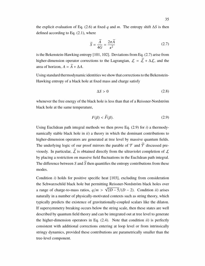
35

the explicit evaluation of Eq. (2.6) at fixed q and m. The entropy shift ∆S is thendefined according to Eq. (2.1), where

S =A

4G=

2π Aκ2

(2.7)

is the Bekenstein-Hawking entropy [101, 102]. Deviations from Eq. (2.7) arise fromhigher-dimension operator corrections to the Lagrangian, L = L + ∆L, and thearea of horizon, A = A + ∆A.

Using standard thermodynamic identitieswe show that corrections to theBekenstein-Hawking entropy of a black hole at fixed mass and charge satisfy

∆S > 0 (2.8)

whenever the free energy of the black hole is less than that of a Reissner-Nordströmblack hole at the same temperature,

F(β) < F(β). (2.9)

Using Euclidean path integral methods we then prove Eq. (2.9) for i) a thermody-namically stable black hole in ii) a theory in which the dominant contributions tohigher-dimension operators are generated at tree level by massive quantum fields.The underlying logic of our proof mirrors the parable of T and T discussed pre-viously. In particular, L is obtained directly from the ultraviolet completion of Lby placing a restriction on massive field fluctuations in the Euclidean path integral.The difference between S and S then quantifies the entropy contributions from thesemodes.

Condition i) holds for positive specific heat [103], excluding from considerationthe Schwarzschild black hole but permitting Reissner-Nordström black holes overa range of charge-to-mass ratios, q/m >

√2D − 5/(D − 2). Condition ii) arises

naturally in a number of physically-motivated contexts such as string theory, whichtypically predicts the existence of gravitationally-coupled scalars like the dilaton.If supersymmetry breaking occurs below the string scale, then these states are welldescribed by quantum field theory and can be integrated out at tree level to generatethe higher-dimension operators in Eq. (2.4). Note that condition ii) is perfectlyconsistent with additional corrections entering at loop level or from intrinsicallystringy dynamics, provided these contributions are parametrically smaller than thetree-level component.

36

small black holes

Planck scale

m

classical GR

large black holes

q

m

Figure 2.1: Black holes ofmaximal charge shown as a function ofmassm and charge-to-mass ratio q/m. Higher-dimension operators induce corrections to the extremalitycondition. If these corrections are positive, then the WGC is automatically satisfied(upper solid curve) since large black holes are unstable to decay to smaller ones. Ifthese corrections are negative (lower solid curve), then theWGCmandates additionallight, superextremal particles to avoid an infinite number of stable extremal blackhole remnants.

While we have only proven the free energy condition in Eq. (2.9) under certainassumptions, its connection to positivity of the entropy shift in Eq. (2.8) is robustand completely general. Furthermore, a trivial corollary to Eq. (2.8) is a positivitycondition on the differential entropy generated at each mass threshold encounteredwhile flowing to the infrared.

Remarkably, classical entropy corrections dominate over quantum contributionsover a broad range of black hole masses still within the regime of validity of theeffective field theory. Within this window, our proof of Eq. (2.8) applies. Sincethe shift in entropy depends on the coefficients of higher-dimension operators,we derive a new class of positivity bounds on the effective field theory. Thisproduces a one-parameter family of constraints on the corresponding coefficientsci labeled by the charge-to-mass ratio of the black hole from which the bound wasderived. Although these conditions are derived from a very particular black holeconstruction, the resulting positivity bounds constrain the coefficients ci in generaland are independent of the background.

37

For the case of highly charged black holes, we obtain a positivity condition on avery specific combination of higher-dimension operator coefficients. Remarkably,it is this exact combination of parameters that also enters into the higher-dimensionoperator correction to the extremality condition for black holes. In particular, wefind that the charge-to-mass ratio for an exactly extremal black hole satisfies

qm− 1 ∝ ∆S, (2.10)

where the right-hand side is positive by Eq. (2.8). Since higher-dimension operatorsdecouple at long distances, the charge-to-mass ratio asymptotes to unity from aboveas we consider larger and larger extremal black holes. Thus, from charge andenergy conservation, it is always possible for an extremal black hole to decay tosmaller extremal black holes of marginally higher charge-to-mass ratio, as shownin Fig. 2.1. Notably, the existence of such states is precisely mandated by the weakgravity conjecture (WGC), which asserts that an Abelian gauge theory consistentlycoupled to gravity must contain a state whose charge exceeds its mass in Planckunits [104], so

qm> 1. (2.11)

The motivation for the WGC is to forbid the existence of an infinite number ofstable states not protected by symmetry. The main result of this paper is thatthis bound is automatically satisfied by small black holes. Though mysterious atfirst glance, the connection between entropy and extremality in Eq. (2.10) actuallyfollows immediately from the near-horizon properties of the metric for a chargedblack hole. As we will show, this connection enables us to straightforwardly extendall of our arguments to the multi-charge generalization of theWGC [105] in arbitrarydimension D.

The WGC is satisfied in numerous concrete examples and is strongly motivated byfolk theorems forbidding exact global symmetries that arise in the vanishing-chargelimit. Moreover, theWGC is a celebrated avatar of the so-called swampland program[104, 106–108], whose ultimate aim is to systematically delineate regions in effectivefield theory space consistent with quantum gravitational ultraviolet completion.

Strictly speaking, a bona fide swampland condition distinguishes between low-energy effective field theories that from an infrared standpoint are otherwise entirelyconsistent. From this perspective it is unclear whether a theory that fails the WGCis in the swampland or merely pathological in a sense that can be diagnosed purelyfrom low-energy considerations. For this reason, a related effort has sought to

38

exclude regions of the low-energy parameter space using infrared consistency, e.g.,constraints from causality, unitarity, and analyticity of scattering amplitudes [108–112]. While theWGChas previously eluded a formal general proof, the present workdemonstrates that it is mathematically equivalent to a certain well-motivated—andin many circumstances provable—property of black hole entropy.

The remainder of this paper is organized as follows. In Sec. 2.2 we prove, givencertain assumptions, that corrections to the Bekenstein-Hawking entropy are posi-tive. Afterwards, in Sec. 2.3 we discuss how various contributions to the black holeentropy arise and estimate their relative size. In order to constrain the coefficients ofhigher-dimension operators, we restrict to black holes within a certain mass range.Next, in Sec. 2.4 we present the perturbative solution for a charged black hole in thepresence of higher-dimension operators. We then compute the black hole entropyin Sec. 2.5 and translate the positivity condition on entropy into a new class ofbounds on higher-dimension operator coefficients in Sec. 2.6. After discussing theimplications of these results for the WGC, we conclude in Sec. 2.7.

2.2 Proof of ∆S > 0In this section, we study corrections to the Bekenstein-Hawking entropy of a ther-modynamically stable black hole at fixed mass and charge. We prove that thesecontributions are positive whenever they come from higher-dimension operatorsgenerated at tree level by quantum fields.

AssumptionsLet us state our assumptions explicitly. First, we assume the existence of quantumfields φ at a characteristic mass scale mφ Λ, where Λ is the energy scale at whichquantum field theory breaks down. This parametric separation is required so thatquantum field theory has some regime of validity. By the usual rules of effectivefield theory, the higher-dimension operators in Eq. (2.4) receive small contributionssuppressed by the cutoff Λ. In general, Λ can be parametrically smaller than thePlanck scale.

Second, we assume that the φ degrees of freedom couple to photons and gravitonssuch that integrating them out generates the higher-dimension operators in Eq. (2.4)classically, i.e., at tree level. Since mφ Λ, these states induce the dominantcontributions to the higher-dimension operators in Eq. (2.4). Specifically, the cor-responding operator coefficients scale as ci ∝ 1/m2

φ 1/Λ2 since tree-level φexchange is always accompanied by a single factor of 1/m2

φ coming from the propa-

39

gator denominator. Thus, effects arising from the cutoff Λ will be negligible in anycontext in which quantum field theory is applicable.

As noted previously, states like φ are a common feature in string theory, whose lowenergy spectrum includes particles like the dilaton and moduli, which are masslessin the supersymmetric limit. In the presence of supersymmetry breaking, these flatdirections are lifted, thus inducing masses mφ Λ, where Λ is the string scale.

While our arguments are perfectly consistent with a scale Λ far below the Planckscale, wewill frequently refer to pureEinstein-Maxwell theory and the pureReissner-Nordström solution as a baseline of comparison. We do so entirely out of conve-nience and not because any component of our argument requires that quantum fieldtheory be applicable up to the Planck scale. Hence, in an abuse of nomenclature,we hereafter refer to the higher-dimension operator contributions of order 1/m2

φ

as corrections to pure Einstein-Maxwell theory, bearing in mind that we actuallymean pure Einstein-Maxwell theory plus contributions of order 1/Λ2, which areparametrically smaller than all the contributions of interest.

Third, we focus on black holes that are thermodynamically stable, i.e., have positivespecific heat. As we will see, this is necessary for technical reasons so that we canexploit certain properties of the Euclidean path integral.

Positivity ArgumentConsider a positively charged black hole of mass M and charge Q perturbed byhigher-dimension operator corrections in general spacetime dimension D. As wewill show in detail in Sec. 2.4, the perturbed metric gµν = gµν + ∆gµν can becomputed from the perturbed Lagrangian L = L + ∆L, where unless otherwisestated all quantities are expressed as perturbations on a Reissner-Nordström blackhole of the same mass M and charge Q in pure Einstein-Maxwell theory.

From the perturbed entropy we can define the corresponding inverse temperatureβ = ∂M S, which we write as

β = β + ∆β, (2.12)

where β = ∂M S is the inverse temperature of the Reissner-Nordström black holeand ∆β = ∂M∆S is the shift of the inverse temperature. The latter appears becausehigher-dimension operators will in general change the temperature of a black holeat a fixed mass and charge.

Next, we compute the free energy F(β) of the perturbed black hole in a canonical

40

ensemble at inverse temperature β. The free energy is calculated from the Euclideanpath integral,

e−βF(β) = Z(β) =∫

d[g]d[A] e−I[g,A], (2.13)

where g and A are integration variables running over metric and gauge field configu-rations. The Euclidean action I = I+∆I is the spacetime integral of theWick-rotatedLagrangian plus boundary terms appropriate to our choice of the canonical ensemble[113]. Here, the boundary conditions at asymptotic infinity are defined by period-icity β in Euclidean time, with a total electric flux Q at the boundary [114], thoughwe suppress all dependence on the latter throughout.

By assumption, the higher-dimension operators in the low-energy effective theoryare dominated by tree-level contributions from heavy fields. The Euclidean pathintegral including these ultraviolet modes is∫

d[g]d[A]d[φ] e−IUV[g,A,φ] =

∫d[g]d[A] e−I[g,A], (2.14)

where φ is a collective integration variable running over all configurations of theheavy fields. As a convention, we choose φ = 0 as the boundary condition atasymptotic infinity, thus defining zero as the vacuum expectation value of the fieldin flat space. In the classical limit, the right-hand side of Eq. (2.14) is obtained bysolving the equations of motion for the heavy fields and plugging these solutionsback into the action.

Now consider an alternative field configuration that instead sets all the heavy fieldsto zero, thus rendering themnon-dynamical. This field configuration does not satisfythe equations of motion, but this will have no bearing on the following argument.For this configuration the massive fields are decoupled and their contributions tohigher-dimension operators are set strictly to zero. It is then a simple mathematicalfact that

IUV[g, A, 0] = I[g, A], (2.15)

where the right-hand side is the Euclidean action for pure Einstein-Maxwell theoryfor any choice of metric and gauge field. The statement of Eq. (2.15) encodes ourassumption that the dominant contributions to the higher-dimension operators in theeffective field theory come from heavy fields.

Putting this all together, we obtain a simple inequality relating the free energy of the

41

perturbed black hole and a Reissner-Nordström black hole at the same temperature,3

− log Z(β) = IUV[gβ, Aβ, φβ] < IUV[gβ, Aβ, 0] = I[gβ, Aβ] = − log Z(β). (2.16)

To obtain the first equality we compute log Z(β) via the saddle-point approximation.Here gβ, Aβ, and φβ are the solutions to the classical equations of motion with sub-scripts to emphasize their consistency with boundary conditions enforcing inversetemperature β. By definition, IUV[gβ, Aβ, φβ] extremizes the Euclidean action. Thesubsequent inequality then holds if this extremum is also a local minimum, in whichcase off-shell field configurations slightly displaced from the classical solutions willincrease the Euclidean action. For this off-shell field configuration we choose thepure Reissner-Nordströmmetric gβ subject to the same boundary condition dictatinginverse temperature β, while pinning all heavy fields to zero. Since this configura-tion differs only marginally from the true solution of the equations of motion, thedisplacement from the local minimum will be tiny as required. From Eq. (2.15)we see that the resulting expression is formally equal to the Euclidean path integralfor pure Einstein-Maxwell theory evaluated on the Reissner-Nordström background.Using the saddle-point approximation once more, we obtain the final equality with− log Z(β), which is β times the free energy F(β) for a Reissner-Nordström blackhole at inverse temperature β.

Crucially, log Z(β) does not correspond to the free energy of a Reissner-Nordströmblack hole of mass M , which has an inverse temperature β. To relate Eq. (2.16) tothe latter, we plug Eq. (2.12) into the right-hand side of Eq. (2.16), yielding

log Z(β) = log Z(β) − M∂M∆S, (2.17)

where log Z(β) is the free energy of a Reissner-Nordström black hole of mass M

and inverse temperature β. To obtain Eq. (2.17), we inserted the thermodynamicrelation, M = −∂β log Z(β), together with the formula for the inverse temperatureshift, ∆β = ∂M∆S. From the definition of the free energy of the canonical ensemble,we then obtain

log Z(β) = S − βM = (1 − M∂M)S

log Z(β) = S − βM = (1 − M∂M)S,(2.18)

wherewe have used the fact that the perturbed black hole at inverse temperature β hasthe same mass as the unperturbed black hole at inverse temperature β. Combining

3Strictly speaking, the free energy of a black hole is obtained only after subtracting the freeenergy contribution from hot flat space or some other reference spacetime [115]. However, sincelog Z(β) and log Z(β) have the same asymptotic boundary conditions, any such reference dependencewill cancel from either side of Eq. (2.16).

42

Eqs. (2.16), (2.17), and (2.18), we cancel terms to obtain

∆S > 0, (2.19)

establishing our claim. The above argument accords with the natural intuition thatconstrainingmicroscopic states, i.e., heavy fields, to be non-dynamical will decreasethe entropy.

Let us comment briefly on a subtle but important caveat to the above arguments.The inequality in Eq. (2.16) crucially assumes that on the black hole solution theEuclidean action is not just an extremum but specifically a local minimum. Thelatter condition guarantees the stability of the Euclidean action under small off-shell perturbations. As is well known, however, the Euclidean path integral suffersfrom saddle-point instabilities mediated by conformal perturbations of the metricthat are unbounded from below. Fortunately, it was shown in Refs. [116, 117]that these particular modes are actually a gauge artifact. For a certain orthogonaldecomposition of the metric, the offending conformal mode can be completelydecoupled from the physical degrees of freedom. With an appropriate contour ofintegration it is then possible to path integrate over this mode to yield a convergentfinal expression.

Later on, an analysis of the Euclidean Schwarzschild solution [118] revealed a bonafide instability coming from a certain non-conformal perturbation about the back-ground solution. This result has been interpreted as evidence that this solutionactually describes a tunneling event from a hot background spacetime into a largeblack hole [119, 120]. Later analyses [121–123] support these claims and moreovershow a direct correlation between the existence of negative modes and the thermo-dynamic instability that arises from negative specific heat. To our knowledge, in allcases considered these saddle-point instabilities disappear when the specific heat ispositive, which for example in D = 4 requires a black hole with q/m >

√3/2 in

natural units.

For the remainder of this paper we restrict to black holes within this thermodynami-cally stable window of charge-to-mass ratios so that the extremum of the Euclideanaction is a local minimum rather than a saddle point and our proof of Eq. (2.19)applies. Crucially, this range of parameters includes highly charged black holes, sothe results of this section can be used in our discussion of the WGC later on.4

4The stability results of Refs. [116–123] were obtained in the context of pure gravity andEinstein-Maxwell theory. However, they should also apply in the presence of additional heavy fields,

43

We believe that Eq. (2.19) is likely true even after relaxing some of the assumptionsoutlined in Sec. 2.2, specifically those requiring a tree-level quantum field theoreticultraviolet completion. In particular, from Eqs. (2.17) and (2.18) it is obvious thatthe positivity condition in Eq. (2.19) is mathematically equivalent to an inequalityof free energies,

F(β) < F(β), (2.20)

which says that the free energy of the perturbed black hole is less than that of aReissner-Nordström black hole at the same temperature. Here we emphasize thatthe former is computed in the theory defined by L and the latter corresponds to L.It is quite possible that the free energy condition in Eq. (2.20) holds in completegenerality, e.g., including quantum corrections.

Explicit ExampleIt is instructive to examine the above arguments for the explicit example of a mas-sive, gravitationally-coupled scalar field. The Euclidean action for the ultravioletcompletion is5

IUV[g, A, φ] =∫

dD x√g

[−

12κ2 R +

14

FµνFµν

+(aφκ

R + bφκFµνFµν)φ +

12∇µφ∇

µφ +12

m2φφ

2],

(2.21)where out of notational convenience the hatted convention employed previously isdropped. . The coupling constants aφ and bφ are dimensionless and have indefinitesign. The classical solution for φ is

φ =1

∇2 − m2φ

(aφκ

R + bφκFµνFµν). (2.22)

Plugging back into the Euclidean action, we obtain

I[g, A] =∫

dD x√g

[−

12κ2 R +

14

FµνFµν −1

2m2φ

(aφκ

R + bφκFµνFµν)2

], (2.23)

which at low energies only produce small corrections to the leading-order black hole solutions. Theprecise crossover from positive to negative specific heat may be slightly shifted by the effects of thecorresponding higher-dimension operators but this has no impact on the thermodynamic stability ofhighly charged black holes, which are safely within this window.

5Here we ignore boundary terms since we will be interested only in the low-energy correctionsgenerated from integrating out heavy fields. These states produce higher-derivative effective opera-tors whose effects fall off quickly with distance and are thus subdominant to bulk action contributions.

44

where all gradient terms from the φ solution are negligible in the low-energy limit.Next, consider the Euclidean action for the full theory, given a field configurationwhere φ is set strictly to zero. The resulting expression is the Euclidean action forpure Einstein-Maxwell theory,

IUV[g, A, 0] =∫

dD x√g

[−

12κ2 R +

14

FµνFµν

]= I[g, A]. (2.24)

Putting this all together, we learn that

I[g, A] < I[g, A] < I[g, A]. (2.25)

The first inequality follows because the action is minimized on the solutions to theclassical equations of motion for thermodynamically stable black holes. The secondinequality follows because Eq. (2.23) differs from Eq. (2.24) by a negative-definitecontribution. This relation between Euclidean actions then implies Eq. (2.20) in thesaddle-point approximation.

Unitarity and MonotonicityFrom Sec. 2.2 it is clear that the entropy inequality ∆S > 0 is very closely relatedto unitarity. In particular, the relative signs derived in the previous example hingedcritically on the absence of tachyons or ghosts in the ultraviolet completion. Thisis not so surprising, since the presence of such pathologies introduce saddle-pointinstabilities on a general background, be it flat space or a black hole. It would beinteresting to draw a direct connection between our results and previous discussionsof unitarity and analyticity [108, 124].

There is also an interesting connection between our results and monotonicity theo-rems along renormalization group flows [125]. Our proof of ∆S > 0 was framedin terms of integrating out all heavy fields at once. However, if the spectrum ofparticles is hierarchical, then this logic can be applied at each mass threshold insequence. The total entropy shift is then

∆S =∫ IR

UVdS, (2.26)

where the differential entropy dS > 0 contributed by each state is positive. Extrap-olating from this classical result, it is reasonable to conjecture that such a positivitycondition persists at the quantum level. Indeed, as we will see in Sec. 2.6, therenormalization of pure Einstein-Maxwell theory accords with this expectation.

45

It is known that the quantum entropy corrections computed from the Euclidean pathintegral are in close relation with the entanglement entropies of the correspondingmodes, where the horizon is the entangling surface (see Refs. [126, 127] and refer-ences therein). Since entanglement entropy is intrinsically positive, so too are thequantum entropy corrections, to the extent to which they are equivalent. We willcomment on this connection in more detail in Sec. 2.3.

2.3 Classical vs. QuantumUp until now we have focused on classical corrections to the entropy, ignoring allloop effects. As we will see, there exists a regime of black hole masses in which theclassical contributions dominate over the quantum. In this case, ∆S > 0 accordingto the proof presented in the previous section. In what follows, we estimate andcompare the characteristic size of the leading tree-level and loop-level correctionsto the black hole entropy.

Leading ContributionsFor concreteness, consider a scalar φ of mass mφ. As per the assumptions ofthe previous section, we assume that this field has the usual minimal couplingto gravitons but also direct couplings to the curvature and electromagnetic fieldstrength. Conservatively, we assume that these couplings are at least of gravitationalstrength, so the interactions go as ∼ φR/κ and ∼ κφF2. Here it will be convenientto define a set of rescaled higher-dimension operator coefficients,

d1,2,3 = κ2c1,2,3, d4,5,6 = c4,5,6, d7,8 = κ

−2c7,8, (2.27)

which are the dimensionally natural basis in which to express quantities. All ofthese rescaled coefficients have mass dimension [di] = −2.

Tree Level. The dominant contributions coming from tree-level φ particle exchangeenter as corrections to the R2, RF2, and F4 operators of size

δ(di) ∼1

m2φ

(tree). (2.28)

Here each contribution scales with a factor of 1/m2φ coming from the φ propagator

denominator.

Loop Level. First, let us consider loop corrections involving purely gravitational in-teractions. At one loop, the leading contributions enter through the renormalization

46

of the gravitational constant,

δ(κ−2) ∼ mD−2φ (loop), (2.29)

which follows straightforwardly from dimensional analysis. At loop level, gravita-tional interactions also yield contributions to higher-dimension operators,

δ(di) ∼ κ2mD−4

φ (loop), (2.30)

which are always subdominant to Eq. (2.28).

Loops involving gauge interactions will similarly renormalize the gauge coupling aswell as the higher-dimension operator coefficients, yielding contributions that scaleas Eq. (2.29) and Eq. (2.30) but with enhancement factors proportional to the charge-to-mass ratios of fundamental charged particles. In principle, these contributionscan dominate. For example, in the standard model, the leading contributions to theEuler-Heisenberg Lagrangian come from loops of electrons. However, as shownin Ref. [109], this only happens when there are fundamental charged particles withlarge charge-to-mass ratios. In this case there is no claim to prove, since WGC isalready satisfied. For this reason, we restrict our consideration to theories where allfundamental charged particles fail or are near the WGC bound without satisfying it.In this limit gauge interactions are of the same strength as gravitational interactionsso the leading tree-level and loop-level corrections from both scale as in Eq. (2.28)and Eq. (2.29).

Region of InterestFrom Eqs. (2.28), (2.29), and (2.30), we can estimate the corresponding correctionsto the black hole entropy, which takes the schematic form

S ∼ρD−2

κ2 + ρD−2mD−2

φ + ρD−4mD−4φ +

ρD−4

κ2m2φ

+ · · · , (2.31)

where ρ is the radius of the black hole. The first term is the Bekenstein-Hawkingentropy, the second term is the quantum correction to the gravitational constant, andthe third and fourth terms are the quantum and classical corrections to the higherdimension operators, respectively. Demanding that classical entropy correctionsdominate over all quantum corrections requires that

ρ 1

κmD/2φ

. (2.32)

47

Crucially, sincemφ is much smaller than the Planck scale, this constraint is consistentwith ρ 1/mφ, which is necessary to remain within the regime of validity of theeffective field theory. For the remainder of this paper we focus on this regime ofblack hole masses.

Before moving on, let us comment briefly on the expectation of positivity for thequantumentropy corrections. While our results only rely on positivity of the classicalcontribution, it is reasonable to conjecture that the same might apply to quantumcorrections. It is known, however, that the quantum contributions in Eq. (2.30) haveindefinite sign and in D = 4 these correspond towell-studied logarithmic correctionsto black hole entropy [128–131]. Nevertheless, these signs do not matter becausewe have already shown that these corrections are parametrically subdominant tothe contributions from Eq. (2.29) related to the renormalization of the gravitationalconstant.

Meanwhile, corrections of the latter type have also been computed via heat kernelmethods and found to be positive for minimally-coupled spin 0 and 1/2 particlesbut negative for spin 0 particles with non-minimal couplings [132] as well as spin 1and spin 2 particles [133, 134]. There is, however, a longstanding debate over thephysical meaning of these negative corrections. They indicate a naivemismatchwithcalculations of quantum field theoretic entanglement entropy, which is manifestlypositive. While these contributions have been understood as the entanglement ofcertain edge modes [135, 136], the sign of the leading power-law divergence wasalso shown to be regulator-dependent. In general, these negative corrections areformally power-law divergent and scheme-dependent and such quantities should beat least partly absorbed into the renormalized gravitational constant [128, 134, 137,138]. For a consistent ultraviolet completion, all divergences will disappear andthe residual corrections will be finite. On physical grounds, it is expected that, ifproperly regulated, these quantum entropy corrections will be manifestly positive asexpected from the manifest positivity of entanglement entropy.

2.4 Black Hole SpacetimeWe now turn to the study of a spherically symmetric, positively charged black holeof mass M and charge Q in the presence of low-energy corrections to pure Einstein-Maxwell theory. For simplicity, we restrict to D = 4 dimensions for the remainderof the body of this paper, but all of our results generalize to arbitrary spacetimedimension D ≥ 4, as shown in App. A.1.

48

Our aim is to derive new bounds on the higher-dimension operator coefficients ci.As noted previously, this restricts our consideration to black holes large enough thatthe effective field theory is valid but small enough to satisfy Eq. (2.32), so 1/mφ

ρ 1/κm2φ, where mφ is the mass scale of the new states. This range always

exists provided there is a parametric separation between mφ and the Planck scale.Furthermore, we consider the thermodynamically stable regime where q/m >

√3/2

so the specific heat is positive.

Note that the mass and charge are defined at spatial infinity. Since we will onlyconsider static spacetimes, the ADM and Komar formulations of these quantitiesare equivalent. Explicitly, the Komar mass and charge are6

M ∼1κ2

∫i0

nµσν∇µKν and Q ∼∫

i0nµ∇νFµν, (2.33)

where the integral region i0 is spatial infinity, n is the unit timelike normal vector,σ is the unit spatial outward-pointing normal vector, and K is the timelike Killingvector. Since the integral is evaluated at spatial infinity, only the leading behaviorat large r contributes to these expressions. Because higher-dimension operatorscorrect the metric and gauge field at subleading order in r , they do not affect thedefinition of the asymptotic mass and charge.

Unperturbed SolutionThe unperturbed theory is described by the Lagrangian for Einstein-Maxwell theoryin Eq. (2.3). For notational convenience we will sometimes describe the mass andcharge in natural units of the gravitational constant,7

m =κ2M8π

and q =κQ

4√

2π. (2.34)

We also define the extremality parameter

ξ =

√1 −

q2

m2 ,(2.35)

6Here we take all black holes to be of definite mass even though in practice they have a smallwidth given by their inverse lifetime. For instance, as classically stable objects, black holes canonly decay quantum mechanically via Hawking emission and Schwinger pair production processes,which are suppressed by additional factors of the gravitational constant. Moreover, decays intosmaller black holes will proceed via non-perturbative gravitational effects, which are exponentiallysuppressed.

7In D dimensions, the mass dimensions of various quantities are [κ2] = 2 − D, [R] = 2,[F] = D/2, [M] = 1, [Q] = 2 − D/2, [m] = [q] = 3 − D, [c1,2,3] = D − 4, [c4,5,6] = −2, [c7,8] = −D,and [di] = −2.

49

where a neutral black hole corresponds to ξ = 1 and an extremal black hole corre-sponds to ξ = 0. As noted previously, we will consider black holes with positivespecific heat, corresponding to q/m >

√3/2, or equivalently, ξ < 1/2.

The solution is the Reissner-Nordström black hole, whose metric takes the staticand spherically symmetric form

ds2 = gµνdxµdxν = − f (r)dt2 +1

g(r)dr2 + r2dΩ2, (2.36)

where the unperturbed metric components are

f (r) = g(r) = 1 −2mr+

q2

r2(2.37)

and the unperturbed electromagnetic field strength is

Fµνdxµ ∧ dxν =Q

4πr2 dt ∧ dr . (2.38)

The unperturbed event horizon is the outer horizon of the Reissner-Nordström blackhole and is located at the radius r = ρ, where

ρ = m +√

m2 − q2 = m(1 + ξ). (2.39)

The absence of a naked singularity implies that the charge is bounded by the in-equality

qm≤ 1, (2.40)

which is saturated in the case of an extremal black hole.

Perturbed SolutionIn the presence of the higher-dimension operators in Eq. (2.4), the perturbed metrictakes the form

ds2 = gµνdxµdxν = − f (r)dt2 +1

g(r)dr2 + r2dΩ2, (2.41)

where the metric components are complicated functions of the coefficients ci. How-ever, as shown in Refs. [139, 140], it is straightforward to compute corrections tothe Reissner-Nordström solution order-by-order in ci. Following the prescription inRef. [139] applied to the higher-dimension operators in Eq. (2.4), we find that atfirst order in ci the radial component of the metric is

g(r) = 1 −2mr+

q2

r2 −q2

r6

45(d2 + 4d3)(6q2 − 15mr + 10r2)

+8d4(3q2 − 7mr + 4r2) +45

d5(11q2 − 25mr + 15r2)

+45

d6(16q2 − 35mr + 20r2) +85(2d7 + d8)q2

,

(2.42)

50

where the coefficients di are defined in terms of ci in Eq. (2.27).

2.5 Calculation of EntropyWald Entropy FormulaWe now compute the entropy corrections to black holes of size much greater thanthe Compton wavelengths of the heavy modes. A major advantage of this approachis that the effects of all short-distance degrees of freedom are encoded purely byhigher-dimension operators. Moreover, even though these states are absent from thelow-energy theory, their contributions to the entropy are fully accounted for by theWald formula in Eq. (2.6).

For a spherically symmetric spacetime, the integral in Eq. (2.6) is trivial, yielding

S = −2πAδL

δRµνρσεµνερσ

gµν, ρ

, (2.43)

where all quantities are evaluated for the perturbed metric and perturbed horizonradius, ρ = ρ + ∆ρ. The perturbed horizon area is A = 4πρ2 and the binormal is

εµν(r) =

√f (r)g(r)(δtµδ

rν − δ

rµδ

tν). (2.44)

Expanding the area A = A+ ∆A and the Lagrangian L = L + ∆L in perturbations,we obtain

S = −2π

(A

δL

δRµνρσ+ A

δ∆L

δRµνρσ+ ∆A

δL

δRµνρσ+ · · ·

)εµνερσ

gµν, ρ

, (2.45)

where A = 4πρ2 and the ellipses denote terms that are higher order in perturbations.The first term is straightforwardly obtained by differentiating Eq. (2.3) with respectto the Riemann tensor,

δL

δRµνρσ=

12κ2g

µρgνσ, (2.46)

where the proper (anti)symmetrization of indices on the right-hand side is implicit.Since the binormal is normalized as εµνε µν = −2, the first term in Eq. (2.45) issimply the unperturbed black hole entropy S defined in Eq. (2.7). Moving this termto the left-hand side of Eq. (2.45), we obtain an expression for the difference inentropies,

∆S = ∆SI + ∆SH, (2.47)

51

split into an "interaction” and "horizon” contribution. Becausewe areworking at firstorder in perturbations, both of these terms should be evaluated on the unperturbedmetric and horizon radius. The interaction contribution,

∆SI = −2π Aδ∆L

δRµνρσεµνερσ

gµν, ρ

, (2.48)

appears because the interactions of photons and gravitons are modified at lowenergies. Meanwhile, the horizon contribution,

∆SH = −2π∆AδL

δRµνρσεµνερσ

gµν, ρ

=2πκ2 ∆A, (2.49)

is present because higher-dimension operators modify the black hole background,thus shifting the location of the horizon. Here we have substituted in Eq. (2.46) towrite the right-hand side of this expression as simply the shift of the horizon area.

Interaction ContributionTo obtain the interaction contribution to the entropy shift we compute

δ∆L

δRµνρσ= 2c1Rgµρgνσ + 2c2Rµρgνσ + 2c3Rµνρσ

+ c4FαβFαβgµρgνσ + c5FµαFραgνσ + c6FµνFρσ,

(2.50)

where proper (anti)symmetrization on indices is left implicit as before. Substitutingthe unperturbed black hole background into Eq. (2.50) and evaluating Eq. (2.48),we obtain

∆SI = S ×2

m2(1 + ξ)3[8d3 − 2(1 − ξ)(d2 + 6d3 + 2d4 + d5 + 2d6)] , (2.51)

written in terms of the coefficients defined in Eq. (2.27). Setting ξ = 1 in ourexpression for ∆SI in Eq. (2.51) agrees with the expressions in Ref. [141] as well astheir generalization to arbitrary dimension in Ref. [142].

Horizon ContributionThe horizon contribution to the entropy shift depends on the location of the perturbedhorizon. Since the spacetime is static, the horizon is determined by zeros of themetric components f (r) and g(r) defined in Eq. (2.41). On general grounds, f (r)

and g(r) have coincident zeros since otherwise the spacetime would contain a regionwith non-Lorentzian signature. Moreover, we have verified by explicit calculationthat f (r) and g(r) share the same zeros at first order in perturbations.

52

The perturbed horizon is located at radius ρ = ρ + ∆ρ. To compute ρ, we expandg(r) = g(r) + ∆g(r) at first order in perturbations, as defined in Eq. (2.42). Theperturbed horizon radius then satisfies the equation

0 = g(ρ) = g(ρ) + ∆g(ρ) + ∆ρ ∂ρg(ρ). (2.52)

The first term on the right-hand side vanishes by the definition of the unperturbedhorizon radius. Solving for the horizon shift, we find

∆ρ = −∆g(ρ)

∂ρg(ρ). (2.53)

At first order, the perturbed horizon area is then given by

∆A = A − A = 8πρ∆ρ = −8πρ∆g(ρ)∂ρg(ρ)

. (2.54)

Inputting the perturbed metric in Eq. (2.42) and evaluating Eq. (2.49), we obtain

∆SH = S ×4(1 − ξ)

5m2ξ(1 + ξ)3[(1 + 4ξ)(d2 + 4d3 + d5 + d6) + 10ξd4 + 2(1 − ξ)(2d7 + d8)].

(2.55)Note that the horizon contribution to the entropy shift is divergent in the ξ → 0 limitcorresponding to an extremal black hole. Physically, this occurs because the innerand outer horizons become degenerate, so ∂ρg(ρ) → 0. In this case, Eq. (2.52)implies that for some fixed contribution ∆g(ρ) from higher-dimension operators,the horizon must shift by a parametrically large amount ∆ρ in order to maintain thehorizon condition.

Of course, the strict ξ → 0 limit is pathological since this produces an infinite entropyshift, signaling a breakdown of perturbation theory. Demanding that the shift inentropy be much smaller than the unperturbed entropy, we obtain the constraint

ξ |di |

m2 .(2.56)

As shown in Eq. (2.32), the classical effects of higher-dimension operators areonly dominant over the quantum for black hole radii smaller than a certain value,ρ 1/κm2

φ. Using that di ∼ 1/m2φ for a tree-level ultraviolet completion, Eq. (2.56)

becomes ξ κ2m2φ.

Perturbativity also requires that the shift in the inverse temperature ∆β be subdomi-nant to the background inverse temperature β of the unperturbedReissner-Nordströmblack hole. As a consistency check, we have verified that β = ∂M S agrees with the

53

surface gravity of the perturbed black hole metric. For highly charged black holes,the unperturbed inverse temperature goes as β ∼ m/ξ while ∆β ∼ di/mξ3. De-manding that the correction be smaller than the leading contribution, ∆β β, weobtain the stronger condition

ξ |di |

1/2

m. (2.57)

Combining this with the upper bound on ρ from Eq. (2.32) and the scaling of di, weobtain

ξ κmφ. (2.58)

Thus, it is always possible to take the limit of a highly charged black hole, ξ 1,provided the mass scale mφ of the heavy fields is far below the Planck scale as wehave assumed throughout.

2.6 New Positivity BoundsGeneral BoundsThe total entropy shift ∆S = ∆SI + ∆SH is obtained by adding Eq. (2.51) andEq. (2.55), yielding

∆S = S ×4

5m2ξ(1 + ξ)3×[

(1 − ξ)2(d2 + d5) + 2(2 + ξ + 7ξ2)d3 + (1 − ξ)(1 − 6ξ)d6 + 2(1 − ξ)2(2d7 + d8)].

(2.59)As proven in Sec. 2.2, the entropy shift is positive under the assumptions we havestated. Combining Eq. (2.8) and Eq. (2.59), we obtain a family of positivity bounds,

(1 − ξ)2d0 + 20ξd3 − 5ξ(1 − ξ)(2d3 + d6) > 0, (2.60)

where we have defined the parameter

d0 = d2 + 4d3 + d5 + d6 + 4d7 + 2d8. (2.61)

The bound in Eq. (2.60) is the main result of this work: a consistency conditionon the coefficients of higher-dimension operator corrections to Einstein-Maxwelltheory following from the positivity of corrections to the black hole entropy. Thegeneralizations of Eqs. (2.59), (2.60), and (2.61) to arbitrary dimension D are derivedand presented in Eqs. (A.18), (A.19), and (A.20) in App. A.1.

As discussed in Sec. 2.2, our proof of ∆S > 0 applies to thermodynamically stableblack holes, restricting consideration to the window ξ ∈ (0, 1/2). The full space ofbounds over this range defines a convex region in the space of coefficients di. Thus

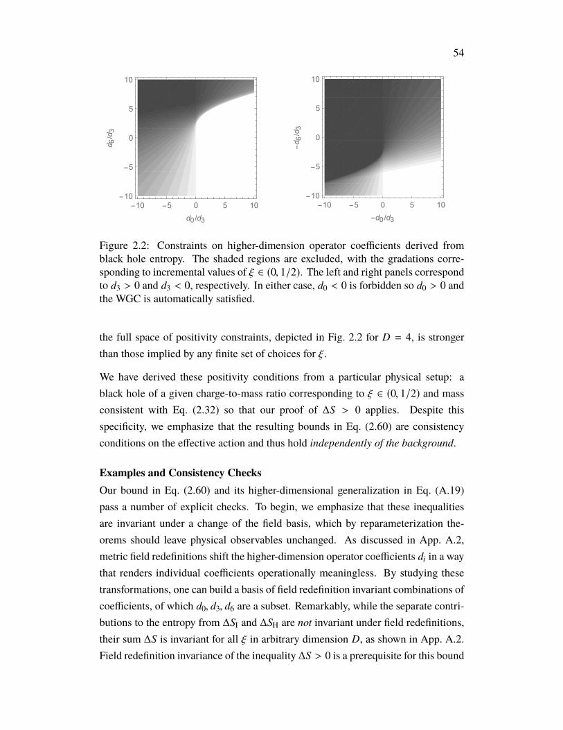
54

-10 -5 0 5 10-10

-5

0

5

10

-d0 /d3

-d6/d3

-10 -5 0 5 10-10

-5

0

5

10

d0 /d3

d 6/d3

Figure 2.2: Constraints on higher-dimension operator coefficients derived fromblack hole entropy. The shaded regions are excluded, with the gradations corre-sponding to incremental values of ξ ∈ (0, 1/2). The left and right panels correspondto d3 > 0 and d3 < 0, respectively. In either case, d0 < 0 is forbidden so d0 > 0 andthe WGC is automatically satisfied.

the full space of positivity constraints, depicted in Fig. 2.2 for D = 4, is strongerthan those implied by any finite set of choices for ξ.

We have derived these positivity conditions from a particular physical setup: ablack hole of a given charge-to-mass ratio corresponding to ξ ∈ (0, 1/2) and massconsistent with Eq. (2.32) so that our proof of ∆S > 0 applies. Despite thisspecificity, we emphasize that the resulting bounds in Eq. (2.60) are consistencyconditions on the effective action and thus hold independently of the background.

Examples and Consistency ChecksOur bound in Eq. (2.60) and its higher-dimensional generalization in Eq. (A.19)pass a number of explicit checks. To begin, we emphasize that these inequalitiesare invariant under a change of the field basis, which by reparameterization the-orems should leave physical observables unchanged. As discussed in App. A.2,metric field redefinitions shift the higher-dimension operator coefficients di in a waythat renders individual coefficients operationally meaningless. By studying thesetransformations, one can build a basis of field redefinition invariant combinations ofcoefficients, of which d0, d3, d6 are a subset. Remarkably, while the separate contri-butions to the entropy from ∆SI and ∆SH are not invariant under field redefinitions,their sum ∆S is invariant for all ξ in arbitrary dimension D, as shown in App. A.2.Field redefinition invariance of the inequality ∆S > 0 is a prerequisite for this bound

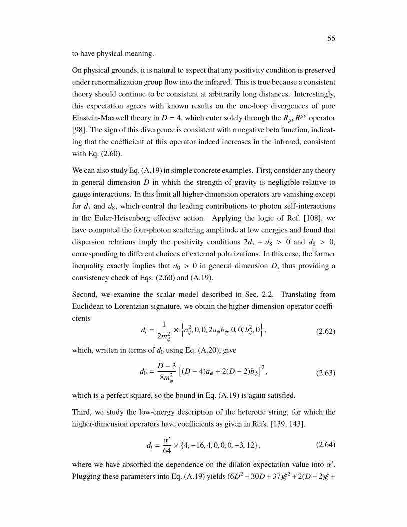
55

to have physical meaning.

On physical grounds, it is natural to expect that any positivity condition is preservedunder renormalization group flow into the infrared. This is true because a consistenttheory should continue to be consistent at arbitrarily long distances. Interestingly,this expectation agrees with known results on the one-loop divergences of pureEinstein-Maxwell theory in D = 4, which enter solely through the RµνRµν operator[98]. The sign of this divergence is consistent with a negative beta function, indicat-ing that the coefficient of this operator indeed increases in the infrared, consistentwith Eq. (2.60).

We can also study Eq. (A.19) in simple concrete examples. First, consider any theoryin general dimension D in which the strength of gravity is negligible relative togauge interactions. In this limit all higher-dimension operators are vanishing exceptfor d7 and d8, which control the leading contributions to photon self-interactionsin the Euler-Heisenberg effective action. Applying the logic of Ref. [108], wehave computed the four-photon scattering amplitude at low energies and found thatdispersion relations imply the positivity conditions 2d7 + d8 > 0 and d8 > 0,corresponding to different choices of external polarizations. In this case, the formerinequality exactly implies that d0 > 0 in general dimension D, thus providing aconsistency check of Eqs. (2.60) and (A.19).

Second, we examine the scalar model described in Sec. 2.2. Translating fromEuclidean to Lorentzian signature, we obtain the higher-dimension operator coeffi-cients

di =1

2m2φ

×

a2φ, 0, 0, 2aφbφ, 0, 0, b2

φ, 0, (2.62)

which, written in terms of d0 using Eq. (A.20), give

d0 =D − 38m2

φ

[(D − 4)aφ + 2(D − 2)bφ

]2, (2.63)

which is a perfect square, so the bound in Eq. (A.19) is again satisfied.

Third, we study the low-energy description of the heterotic string, for which thehigher-dimension operators have coefficients as given in Refs. [139, 143],

di =α′

64× 4,−16, 4, 0, 0, 0,−3, 12 , (2.64)

where we have absorbed the dependence on the dilaton expectation value into α′.Plugging these parameters into Eq. (A.19) yields (6D2 − 30D+ 37)ξ2 + 2(D− 2)ξ +

56

2D−5 > 0, which holds for all ξ ∈ (0, 1) and D > 3. Thus, we find that Eq. (A.19) isactually satisfied even beyond the range of thermodynamic stability and the criticaldimension of the string.

The Weak Gravity ConjectureIn the limit of a highly charged black hole we take ξ 1 and our general bound inEq. (2.60) becomes

d0 > 0, (2.65)

with d0 defined in terms of the other di in Eq. (2.61).

As it turns out, this inequality is intimately connected with the extremality conditionfor a black hole. To see why, consider the unperturbed Reissner-Nordström solution,for which the extremal charge-to-mass ratio is z = q/m = 1. In general, quantumcorrections to the gravitational constant and electric charge will renormalize theright-hand side of this condition. Since these contributions affect black holes ofall masses universally, their effects can simply be absorbed into the definitions ofmass and charge. Meanwhile, higher-dimension operators also shift the maximumcharge-to-mass ratio permitted for a physical black hole, i.e., a black hole freefrom naked singularities. In contrast, these corrections are mass-dependent, so theyinduce a physical shift of the extremality condition to z = z + ∆z [139].

To compute this shift, we analyze the metric component g(r, z), interpreted as afunction of both the radius and the charge-to-mass ratio. The shifted horizon isdefined by the condition g(ρ, z) = 0. At linear order in perturbations, this conditionbecomes

0 = g(ρ, z) = g(ρ, z) + ∆g(ρ, z) + ∆ρ ∂ρg(ρ, z) + ∆z ∂zg(ρ, z). (2.66)

Since the unperturbed black hole is extremal, the first and third terms on the right-hand side are zero. Solving for the shift in the charge-to-mass ratio yields

∆z = −∆g(ρ, z)∂zg(ρ, z)

. (2.67)

By explicit calculation, the charge-to-mass ratio shift is

∆z =2d0

5m2 > 0, (2.68)

which is positive according to Eq. (2.65).

As shown in Ref. [139], if ∆z is positive then small black holes automaticallysatisfy the WGC [104], which posits that an Abelian gauge theory consistently

57

coupled to quantum gravity must contain a state with charge-to-mass ratio greaterthan unity. In its original formulation [104], the WGC was presented with severalcompelling justifications. This included overwhelming circumstantial evidencefrom a long list of explicit examples in quantum field theory and string theory.A more direct argument was also presented in the form of an elegant thoughtexperiment involving stable black hole remnants [144–148]. In particular, due tomass and charge conservation, a charged black hole is stable unless there existlighter states with a higher charge-to-mass ratio, into which the black hole candecay. In the infinite-mass limit, the charge-to-mass ratio of an extremal black holeis dictated by the Reissner-Nordström solution and approaches unity. Violation ofthe WGC would then imply the existence of an infinite tower of stable remnantslabeled by the extremal black hole mass, asserted as pathological in Ref. [104].While this thought experiment offers some crucial physical intuition for the WGC,it falls short since there do not exist formal proofs that stable black hole remnantsare actually inconsistent with more established principles like the covariant entropybound. In many cases the number of black hole remnants is very large but stillfinite; furthermore, the states are labeled by distinct charges and are thus in principledistinguishable [149].

On the other hand, if the WGC is satisfied then extremal black holes are unstableto decay. We have shown here that considerations of black hole entropy imply thatthe charge-to-mass ratio of an extremal black hole increases with decreasing size.In particular, higher-dimension operators induce a positive shift of the extremalitybound, but these corrections decouple for large black hole masses. The upshot isthen that an extremal black hole of a given mass can always decay into smallerextremal black holes of a greater charge-to-mass ratio, following the upper curve inFig. 2.1. Our bound in Eq. (2.65)—and thus our proof of the WGC—generalizes toD spacetime dimensions, as shown in App. A.1.

Let us comment on the relation between our results and previous work connectingblack holes and the WGC. First, while the argument in this paper makes criticaluse of extremal black holes, our reasoning is completely different from the originalproposal of Ref. [104], hinging instead on the thermodynamic entropy of blackholes rather than their stability. More recently, the WGC has also been linked to thecosmic censorship conjecture [150]. We leave an analysis of this and its relationshipto black hole entropy for future work.

In other recent studies [149, 151], theWGC has also been evaluated in the context of

58

black hole entropy using methodologies that differ substantially from our own. BothRef. [149] and Ref. [151] examine the leading logarithmic corrections to black holeentropy due to the quantum effects of light matter particles. Such effects are relevantfor black holes of size parametrically smaller than the Compton wavelength of thematter. We, in contrast, consider the opposite regime, which effectively correspondsto a gapped spectrum.

Furthermore, Refs. [149, 151] argue for the inconsistency ofWGC violation throughquite different means: Ref. [149] makes the argument through the appearance ofa low cutoff, while Ref. [151] employs the second law of thermodynamics. It iscrucial to note that our assertion of a positive entropy shift is logically distinct fromthe second law of thermodynamics, which applies to the difference in entropy beforeand after a physical process but within the same physical system. Our constructionis instead based on the positivity of classical entropy corrections proven in Sec. 2.2.

Finally, Refs. [149, 151] and also another interesting approach [152] all considerconcrete models with explicit spectra of charged and neutral scalars and fermions.For this reason, these works at best show that certain WGC-violating theories areinconsistent. This leaves the logical possibility that more complicated theories thatviolate the WGC might still be judged valid by their analyses. In comparison, ourwork applies to large black holes in a general low-energy effective theory, whichis insensitive to the precise details of the spectrum and hence constitutes a model-independent argument for the WGC.

Entropy, Area, and ExtremalityA priori, it is somewhat miraculous that the entropy constraint in Eq. (2.65) isliterally equivalent to the extremality condition in Eq. (2.68). To briefly summarize,we have shown that

∆S ∼ ∆ρ ∼ ∆z > 0, (2.69)

so the low-energy corrections to the near-extremal black hole entropy, area, andextremality condition are all proportional to each other and all positive.

Why does the same combination of coefficients d0 appear in all of these inequalities?As it turns out, this connection is not so mysterious once one considers the perturbedmetric component g(ρ, z) in Eq. (2.66) as a function of the shift in horizon radius∆ρ and the shift in the charge-to-mass ratio ∆z. For a near-extremal black hole offixed charge and mass, we set ∆z = 0 and thus ∆ρ = −∆g/∂ρg. On the other hand,if the charge and mass are free but the unperturbed system is exactly extremal, then

59

the ∆ρ term drops out and the charge-to-mass ratio shift is ∆z = −∆g/∂zg. At thesame time, the radial component of the metric g is by definition spacelike outsidethe horizon, so ∂ρg > 0. Moreover, since g dictates the gravitational potential atlong distances, it decreases with m and thus increases with the charge-to-mass ratio,so ∂zg > 0. This logic implies that ∆ρ and ∆z have the same sign. Since theentropy shift for a near-extremal black hole is dominated by the shift in the horizon,∆S ∼ ∆ρ, we discover that ∆S > 0, ∆ρ > 0, and ∆z > 0 are equivalent bounds.

Conveniently, the above logic immediately extends to themulti-charge generalizationof the WGC proposed in Ref. [105]. For a theory with multiple Abelian factors, thecharge-to-mass ratio defines a vector z in charge space. The WGC then mandatesthat the unit ball representing all possible large black holes be contained within theconvex hull spanned by the set of all z for the lighter states in the theory. Crucially,for a multi-charged black hole, the perturbed metric only depends on the magnitudeof its charge and not the direction. Hence, Eq. (2.66) still applies, provided wedefine z = |z| as the magnitude of the charge-to-mass ratio vector of the black holeand ∆z = ∆z · z/|z| as its shift. Repeating exactly the argument of the previousparagraph, we learn that ∆S > 0, ∆ρ > 0, and ∆z · z > 0 are all equivalent. The lastinequality implies that the extremality condition for a multi-charged extremal blackhole is perturbed so that the corresponding unit ball is expanded outward in everydirection, thus proving the multi-charge version of the WGC given by the convexhull condition in Ref. [105].

2.7 Discussion and ConclusionsIn this paper, we derived a positivity condition on classical corrections to theBekenstein-Hawking entropy. For near-extremal black holes this enforces positivityof a certain linear combination of coefficients of higher-dimension operators. Thisvery same combination of couplings corrects the extremality condition for blackholes so that their charge-to-mass ratios approach unity from above for increasingsize. Large extremal black holes are thus unstable to decay to smaller extremalblack holes. Since the latter have charge-to-mass ratios greater than unity, theyautomatically fulfill the requirement of the WGC.

Our findings leave a number of avenues for future work. First, it would be interest-ing to determine if entropy considerations have any additional implications for theswampland program, for example by introducing new operators in extended theorieslike Einstein-dilaton gravity or by considering black holes embedded in asymptot-

60

ically AdS or dS space, rotating black holes, or black holes of different topologies.Second, one would ideally like to understand the relationship, if any, between theseentropy bounds and other contraints on low-energy dynamics coming from causality,analyticity, and unitarity. Indeed, the positivity of entropy shifts discussed in thispaper stems from state counting in the ultraviolet, which is highly reminiscent ofdispersion relation bounds utilizing the positivity of forward cross-sections [108–111, 124, 153–155] and amplitudes approaches based on the positivity of spectralrepresentations [112, 156, 157].

Acknowledgments

We thank Nima Arkani-Hamed, Raphael Bousso, Sean Carroll, William Cottrell,Daniel Harlow, Tom Hartman, Yasunori Nomura, Hirosi Ooguri, Matthew Reece,Prashant Saraswat, Gary Shiu, Leo Stein, and Aron Wall for helpful discussions.C.C. and J.L. are supported by a Sloan Research Fellowship and DOE Early CareerAward under grant no. DE-SC0010255. G.N.R. is supported by the Miller Institutefor Basic Research in Science at the University of California, Berkeley.

61

C h a p t e r 3

BOOTSTRAPPING HEISENBERG MAGNETS AND THEIRCUBIC INSTABILITY

This chapter is based on S. M. Chester, W. Landry, J. Liu, D. Poland, D. Simmons-Duffin, N. Su and A. Vichi, Bootstrapping Heisenberg Magnets and their CubicInstability, arxiv: 2011.14647 [hep-th].

Abstract: We study the critical O(3) model using the numerical conformal boot-strap. In particular, we use a recently developed cutting-surface algorithm to effi-ciently map out the allowed space of CFT data from correlators involving the leadingO(3) singlet s, vector φ, and rank-2 symmetric tensor t. We determine their scal-ing dimensions to be (∆s,∆φ,∆t) = (0.518942(51), 1.59489(59), 1.20954(23)), andalso bound various OPE coefficients. We additionally introduce a new "tip-finding"algorithm to compute an upper bound on the leading rank-4 symmetric tensor t4,which we find to be relevant with ∆t4 < 2.99056. The conformal bootstrap thusprovides a numerical proof that systems described by the critical O(3) model, suchas classical Heisenberg ferromagnets at the Curie transition, are unstable to cubicanisotropy.

3.1 IntroductionNumerical bootstrap methods [158, 159] (see [160, 161] for recent reviews) haveled to powerful new results in the study of conformal field theories (CFTs). In[4, 5] we developed an approach to large-scale bootstrap problems which allowedfor precise determinations of the CFT data of the 3d critical O(2) model. In thiswork, we continue the exploration of large-scale bootstrap problems by applying thetechnology introduced in [4] to the study of the 3d critical O(3) model.

Concretely, we apply these methods to study correlation functions of the lowest-dimension singlet, vector, and rank-2 scalars in the three-dimensional critical O(3)model. Using the "cutting surface" algorithm introduced in [4], we compute theallowed region for the CFT data of these leading scalar operators. Our results,together with comparisons to results fromMonte Carlo simulations, are summarizedin table 3.1. We also introduce a new algorithm and software implementation calledtiptop, which allows us to efficiently test allowed gaps for other operators across

62

this region. We use it to determine an upper bound on the dimension of the lowest-dimension rank-4 scalar.

The 3d O(3)model is a well-studied renormalization group (RG) fixed point, and itscritical exponents have been computed using many methods, both theoretical andexperimental. This model describes the critical behavior of isotropic magnets, suchas the Curie transition in isotropic ferromagnets, and antiferromagnets at the Néeltransition point. Moreover, since disorder corresponds to an irrelevant perturbation,1the model also describes isotropic magnets with quenched disorder.

One of the main open questions about the O(3) model is its stability under cubicdeformations. The majority of magnets present in nature are indeed not isotropic:this means that the microscopic Hamiltonian describing the system in the ultraviolet(UV) is not invariant under the full O(3) symmetry group but only under a discretesubgroup, such as the cubic symmetry group. This implies that additional termswill be generated at the microscopic level that are invariant under cubic symmetrybut transform in a non-trivial representation of O(3). If any of those deformationsturn out to be relevant, the O(3) fixed point would be unstable and could not bereached without further tuning in the UV theory. The attractive, stable, fixed pointwould instead be the 3d cubic model. Field theory computations and Monte Carlosimulations have shown that these two models have very similar critical exponents:hence, if the cubic perturbation is relevant, it should be very close to marginalityand the RG flow connecting the two theories is very short. We will come back tothis point in section 3.1.

We give a definite answer to the above question: the O(3) model is unstable undercubic deformations. This information is encoded in the dimension of the lowestrank-4 scalar t4, which in the O(3) model satisfies ∆t4 < 3. As we will discuss, thisimplies that the O(3) model is also unstable with respect to the biconal fixed pointwith Z2 ×O(2) symmetry. Relevance of t4 has been previously suggested by MonteCarlo [8] and perturbative expansions [164], but the proximity to marginality andnear degeneracy of the critical exponents between the cubic, biconal, and O(3) fixedpoints makes this a subtle question ideal for the precision and rigor of the conformalbootstrap.

1This is the case in any O(N) model with N ≥ 2.

63

CFT data method value ref

∆s MC 1.5948(2) [7]CB 1.5957(55) [162]CB 1.59488(81) this work

∆φ MC 0.518920(25) [7]CB 0.51928(62) [162]CB 0.518936(67) this work

∆t MC 1.2094(3) [8]CB 1.2095(55∗) [163]CB 1.20954(32) this work

∆t4 MC 2.987(4) [8]CB < 2.99056 this work

λφφs CB 0.5244(11∗) [162]CB 0.524261(59∗) this work

λsss CB 0.499(12∗) [162]CB 0.5055(11∗) this work

λtts CB 0.98348(39∗) this work

λφφt CB 0.87451(22∗) this work

λttt CB 1.49957(49∗) this work

Table 3.1: Comparison of conformal bootstrap (CB) results with previous determi-nations from Monte Carlo (MC) simulations. We denote the leading rank-0, rank-1,rank-2, and rank-4 scalars by s, φ, t, t4, respectively. Bold uncertainties correspondto rigorous intervals from bootstrap bounds. Uncertainties marked with a ∗ indicatethat the value is estimated non-rigorously by sampling points.

Theoretical approaches to the 3d O(3) modelWe start by briefly reviewing past approaches to the 3d O(3) model, includingfield theory studies, Monte Carlo, and past results obtained by conformal bootstraptechniques. We also describe related models and motivate the calculations in thiswork.

The simplest continuum field theory in the O(3) universality class is the theoryof a scalar field ®φ transforming in the fundamental representation of O(3) withLagrangian

L =12|∂ ®φ|2 +

12

m2 | ®φ|2 +g

4!| ®φ|4 . (3.1)

A large negative mass-squared for the scalar induces spontaneous symmetry break-ing and leads to the ordered phase, while a large positive mass-squared leads to

64

the disordered phase. The critical point is achieved by tuning the UV mass so thatthe infrared (IR) correlation length diverges. The β function of the coupling g

has been computed in the ε−expansion and in a fixed-dimension scheme. After aBorel-resummation, both methods predict the existence of an IR stable fixed point.We will review these results in the next sections.

The IR limit of the above field theory captures the same physics as the Heisen-berg model. This model consists of a lattice of classical spins ®Si, which can takevalues on a three-dimensional sphere. The Hamiltonian has only nearest-neighborinteractions:

H = −J∑〈i, j〉

®Si · ®Sj + H∑

i

Si , (3.2)

where we also introduced an external magnetic field H. When the parameter J

is positive, the ground state corresponds to all spins aligned, corresponding toferromagnets. When J < 0, the energy is minimized when neighboring spins areanti-aligned, corresponding to antiferromagnets.

For small J, the line H = 0 separates a ferromagnetic phase from the paramagneticone. This line represents a first-order transition and terminates at a value J = Jc,where the correlation length of the system diverges, and the transition becomessecond order. For J > Jc, there is only a disordered phase. At J = Jc, the theoryin the IR is in the same universality class of the field theory defined in (3.1). Thecritical exponents are related to operator dimensions at the fixed point as

∆φ =1 + η

2, ∆s = 3 −

1ν, ∆t = 3 − Y2 . (3.3)

Here, s ∼ | ®φ|2 denotes the lowest-dimension singlet scalar, while ti j ∼ (φiφ j − trace)denotes the lowest rank-2 scalar. More generically the exponents Yr are associatedto the dimensions of the lowest rank-r scalar operator.2 In the O(N) model, thedimension of the lowest traceless symmetric operator t describes the instability ofthe theory against anisotropic perturbations. Because of this, it plays an importantrole in the description of multicritical phenomena. For instance, the critical behaviornear a bicritical point where two critical lines with O(n1) and O(n2) symmetry meetgivies rise to a critical theory with enlarged O(n1 + n2) symmetry.

The Hamiltonian (3.2) is a simplified model of magnetic interactions, since in areal crystalline solid other interactions are present. For instance, the crystal latticestructure could give rise to magnetic anisotropy. In cubic-symmetric lattices this

2Sometimes in the literature they are replaced by the crossover exponents φr = νYr .

65

effect produces an interaction localized at each lattice point i of the form∑3

k=1(Ski )

4.This perturbation breaks the O(3) global symmetry of the Heisenberg Hamiltonian,and therefore it cannot be generated by an RG transformation. As such, the IR fixedpoint of (3.2) will be described by an O(3) invariant CFT.

O(N) vs. multi-critical models

The O(3) model described above can be generalized to O(N) by promoting ®φ toan N component field. We can also consider the closely related cubic model,which describes the continuum limit of the Hamiltonian (3.2) with the addition ofthe O(N) breaking term

∑Nk=1(S

ki )

4. This interaction is indeed invariant under thesymmetries of a hyper-cubic lattice, namely permutations and reflection of the threeaxes. The field φi, i = 1, . . . , N , transforms in the fundamental representation ofthe permutation group SN . Moreover, each component is odd under a reflection ofthe corresponding axis. The composition of these transformations gives rise to thehypercubic symmetry group CN = ZN o SN .

Compared to (3.1), the Lagrangian of the hypercubic model has an additional termin the potential:

L =12

N∑i=1

((∂µφi)

2 + m2φ2i

)+

g

4!

(N∑

i=1φ2

i

)2

+h4!

N∑i=1

φ4i . (3.4)

The computation of the two β-functions βg and βh reveals the existence of four fixedpoints: the trivial fixed point (g = h = 0), the N decoupled copies of the Isingmodel (h , 0, g = 0), the O(N) fixed point (g , 0, h = 0) and the cubic model(g , 0, h , 0). It is straightforward to see that the first two are unstable since thequartic operator parametrized by g is relevant in both theories.3 Determining whichone of the other two fixed points is stable is a more complicated issue, and it turnsout to be N dependent.

One way to rephrase the above question is to notice that the additional term in (3.4)can be rewritten as

N∑i=1

φ4i =

N∑i=1

tiiii4 +

3N + 2

(N∑

i=1φ2

i

)2

, (3.5)

where ti j kl4 is the traceless symmetric combination of four fields. The added term

in the potential, in O(N) notation, can be written as a combination of a rank-4 field3The case of N decoupled Ising model corresponds to products of operators εi ∼ φ2

i belongingto different copies where 2∆ε < 3 in the Ising model.

66

and a singlet. We know that the singlet is irrelevant at the O(N) fixed point, bydefinition. Thus the stability of the O(N) fixed point or the cubic point is linked tothe value of the dimension of the operator t4.

In theO(2)model the operator t4 is irrelevant. A simple proof of this is to notice thatfor N = 2, as long as h , 0, the cubic Lagrangian can be mapped in the Lagrangianof two decoupled Ising models. This cubic fixed point coincides with the decoupledIsing fixed point, which is unstable. Field theory and Monte Carlo determinationsof the dimension of t4 agree with this argument. This is also consistent with theassumptions made in [4].On the contrary, at large N , the operator t4 is relevant, and the cubic fixed point isstable. Thus, it is important to know at which value N = Nc > 2 the operator t4becomes relevant.

A second closely related model is the multi-critical point with O(n1) × O(n2) sym-metry. A field theory description is given in terms of two sets of scalar fields ®φ1 and®φ2, transforming respectively in the fundamental representation of O(n1) and O(n2),with Lagrangian:

L =12

2∑i=1|∂µ ®φi |

2 +g14!

(| ®φ1 |

2)2+g24!

(| ®φ2 |

2)2+

h4| ®φ1 |

2 | ®φ2 |2 , (3.6)

where we have already set to zero all the mass terms. The analysis of the perturbativeβ functions shows the existence of six fixed points. Some we already know: thefree one (gi = 0, h = 0), the two Wilson Fisher fixed points (g1 , 0, g2 = h = 0 andsame with 1 ↔ 2), the decoupled fixed point (DFP, gi , 0, h = 0), the symmetryenhanced O(n1 + n2) Wilson Fisher fixed point, and lastly the biconal fixed point(BFP). The latter one also has all couplings nonvanishing, but the global symmetryis not enhanced.

The problem of understanding the stable fixed point can be again reduced to studyingthe (ir)relevance of given deformations in the various CFTs. For instance, byinspecting the dimension of the composite operator built out of the lowest dimensionscalar singlets in O(n1) and O(n2) theories, one can conclude that the DFP is stablefor any N = n1 + n2 ≥ 4. It is unstable for N ≤ 3, although the perturbation is closeto being marginal.4

The issue of stability of O(N) vs. the BFP is again related to the dimension of acertain operator. In the Lagrangian formulation, this is a combination of quartic

4The most precise bootstrap determination [4, 162] gives ∆[sZ2 sO(2)]= ∆sZ2

+ ∆sO(2) =

2.92398(23) < 3.

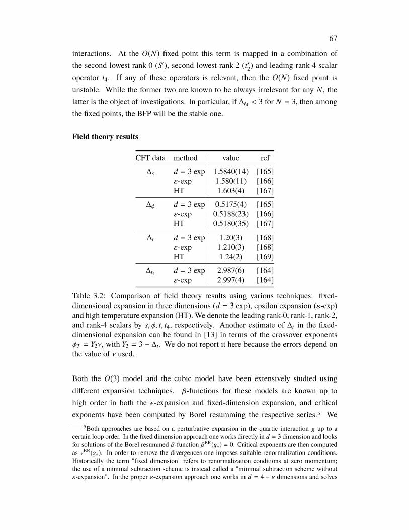
67

interactions. At the O(N) fixed point this term is mapped in a combination ofthe second-lowest rank-0 (S′), second-lowest rank-2 (t′2) and leading rank-4 scalaroperator t4. If any of these operators is relevant, then the O(N) fixed point isunstable. While the former two are known to be always irrelevant for any N , thelatter is the object of investigations. In particular, if ∆t4 < 3 for N = 3, then amongthe fixed points, the BFP will be the stable one.

Field theory results

CFT data method value ref

∆s d = 3 exp 1.5840(14) [165]ε-exp 1.580(11) [166]HT 1.603(4) [167]

∆φ d = 3 exp 0.5175(4) [165]ε-exp 0.5188(23) [166]HT 0.5180(35) [167]

∆t d = 3 exp 1.20(3) [168]ε-exp 1.210(3) [168]HT 1.24(2) [169]

∆t4 d = 3 exp 2.987(6) [164]ε-exp 2.997(4) [164]

Table 3.2: Comparison of field theory results using various techniques: fixed-dimensional expansion in three dimensions (d = 3 exp), epsilon expansion (ε-exp)and high temperature expansion (HT). We denote the leading rank-0, rank-1, rank-2,and rank-4 scalars by s, φ, t, t4, respectively. Another estimate of ∆t in the fixed-dimensional expansion can be found in [13] in terms of the crossover exponentsφT = Y2ν, with Y2 = 3 − ∆t . We do not report it here because the errors depend onthe value of ν used.

Both the O(3) model and the cubic model have been extensively studied usingdifferent expansion techniques. β-functions for these models are known up tohigh order in both the ε-expansion and fixed-dimension expansion, and criticalexponents have been computed by Borel resumming the respective series.5 We

5Both approaches are based on a perturbative expansion in the quartic interaction g up to acertain loop order. In the fixed dimension approach one works directly in d = 3 dimension and looksfor solutions of the Borel resummed β-function βBR(g∗) = 0. Critical exponents are then computedas νBR(g∗). In order to remove the divergences one imposes suitable renormalization conditions.Historically the term "fixed dimension" refers to renormalization conditions at zero momentum;the use of a minimal subtraction scheme is instead called a "minimal subtraction scheme withoutε-expansion". In the proper ε-expansion approach one works in d = 4 − ε dimensions and solves

68

report in table 3.2 the latest results obtained with field theory techniques.

The question of stability of fixed points has also been discussed in the literature. Aswe discussed in the previous section, this question can be addressed in two ways: bycomputing the dimension of the lowest dimension rank-4 scalar in the O(3) model,or by computing the value Nc at which the dimension of the second-lowest rank-0scalar in the cubic model becomes exactly marginal.6 Results from both methodssupport the conclusion that O(3) is unstable while the cubic model is stable. Theformula for Nc in the ε-expansion is [170, 171]:

Nc = 4 − 2ε + 2.58847559ε2 − 5.87431189ε3 + 16.82703902ε4 +O[ε5] , (3.7)

and after resummation gives Nc = 2.89(2).

Analysis of the ε-expansion or fixed-dimension perturbative series in the cubicmodel [168, 172, 173] shows that the critical exponents of the two models are veryclose:

νO(3) − νcubic = 0.0003(3) , ηO(3) − ηcubic = 0.0001(1) . (3.8)

These differences are much smaller than the typical experimental error (e.g., [174]).This makes distinguishing the two models experimentally very challenging. Curi-ously, the first few terms in the of the ε-expansion of the critical exponents in (3.8)are quite different, and it is only after the Borel resummation that the two valuesappear quite close.

Similarly, also the biconalZ2 ×O(2)model and the O(3) critical exponents are veryclose, as the flow connecting the two is driven by the same almost marginal operatoras in the cubic case:

|νO(3) − νBFP | . 0.001 , |ηO(3) − ηBFP | = 0.0005 , |ηO(3) − η′BFP | = 0.0001 ,

(3.9)where ηBFP and η′BFP correspond to the two relevant order parameters chargedrespectively under Z2 or O(2).

the condition β(g∗) = 0 order by order in ε. Plugging the solution g∗(ε) into the expression for thecritical exponent one gets a series in ε that can be Borel resummed. The final critical exponents arethen computed as νε-BR(ε = 1).

6The lowest dimension one corresponds to the mass deformation and is always relevant; thesecond-lowest corresponds to a combination of the two quartic interactions. The orthogonal combi-nation is related to the Lagrangian operator via the equation of motion and is irrelevant.

69

Monte Carlo results

Using Monte Carlo (MC) techniques, it is possible to obtain precise estimatesof the critical exponents for both the O(3) model and the cubic model, as wellas information about their stability. Such determinations can also be improvedwhen combined with finite-size scaling (FSS) or high-temperature expansion (HT)methods. A precise determination of the ν and η critical exponents was made usingMC and FSS methods in [175]. A more precise analysis combining MC with HTtechniques was carried out in [176], while a more precise MC and FSS study wasperformed in [8]. A very precise MC and FSS analysis of an icosahedral model,as well as improved MC and HT analyses were recently presented in [7]. Severalother less precise determinations can be found in [174]. The dimensions relevantto anisotropic perturbations of rank-2,3,4 were computed in [8, 177] using MC andFSS methods, and support the conjecture that the O(3) model is unstable undercubic deformations. These results are summarized in table 3.1.

The conformal bootstrap

Three dimensionalO(3)models have been studied with bootstrapmethods in a seriesof papers [162, 163, 178], first by considering the correlation function 〈φiφ jφkφl〉,where φi is the lowest-dimension scalar transforming in the vector representationof O(N) , and then by also including correlation functions involving the lowest-dimension singlet scalar s. The most precise determination of the critical exponentswas obtained in [162], which isolated a three dimensional region in the space∆φ,∆s, λsss/λφφs = 0.51928(62), 1.5957(55), 1.205(9), under the assumptionthat φi and s are the unique relevant scalar operators in their representations. Inaddition, by scanning over this island, [162] determined themagnitude of the leadingOPE coefficient to be λφφs = 0.5244(11).

Theories invariant under the cubic symmetry groupwere also studied using bootstrapmethods using single correlators [179, 180], and mixed correlators [181, 182]. Inparticular [180] analyzed the bootstrap equations assuming the hypercubic symmetrygroup CN = ZN o SN and observed a series of kinks for various values of N .However, the locations of the kinks in the singlet sector were degenerate withthe O(N) kinks (and hence compatible with (3.8)), likely reflecting a symmetryenhancement in the extremal bootstrap solutions [183–187], while the bounds inother sectors did not seem to be saturated by the cubic model. The mixed-correlatoranalysis of [181, 182] also did not manage to isolate the cubic model but rather

70

found evidence of a new theory, called the "Platonic CFT," with cubic symmetryand operator dimensions not matching any known CFT.

In this work, we study the O(3) model with numerical bootstrap techniques usinga larger system of correlation functions than before: in addition to φi and s, weincorporate the lowest-dimension rank-2 scalar ti j ∼ φ(iφ j). This setup is similarto the one leading to the successful results obtained in [4] for the O(2) model.Following the strategy detailed in [4], we first scan over the three operator dimen-sions ∆φ,∆s,∆t and the OPE coefficients sss, φφs, tts, φφt, ttt (or more preciselytheir ratios) and we determine a three dimensional island in the space of operatordimensions, along with an associated allowed set of OPE coefficient ratios. Next,we compute upper and lower bounds on the magnitude λφφs, as well as on the cur-rent and stress-tensor central charges CJ and CT . Finally, we enlarge the parameterspace to include one more parameter: the dimension of the lowest rank-4 scalar∆t4 . Using the new tiptop algorithm, which we describe in section 3.3, we carveout the allowed region in the enlarged four-dimensional space and obtain an upperbound on ∆t4 .

Structure of this workThe remainder of this work is structured as follows. In section 3.2 we describethe crossing equations and relevant O(3) representation theory. In section 3.3 wedescribe the new tiptop algorithm that we use in order to bound ∆t4 . In section 3.4we describe the results of our numerical bootstrap calculations and in section 3.5we describe directions for future research. Various appendices describe the codeavailability, software setup, details about our tensor structures, and give a list ofallowed and disallowed points that we have computed.

3.2 The O(3) modelCrossing equationsWe begin by describing the representation theory of O(3) = Z2 × SO(3). We labelthe irreducible representations q± of O(3) by the usual SO(3) rank q tensor ofdimension 2q+ 1 for q ∈ 1

2Z≥0, as well as theZ2 parity ±. Tensor products of theseirreps are given by

q1± ⊗ q2

± =

q1+q2⊕qa=|q1−q2 |

qa+ , q1

± ⊗ q2∓ =

q1+q2⊕qa=|q1−q2 |

qa− , (3.10)

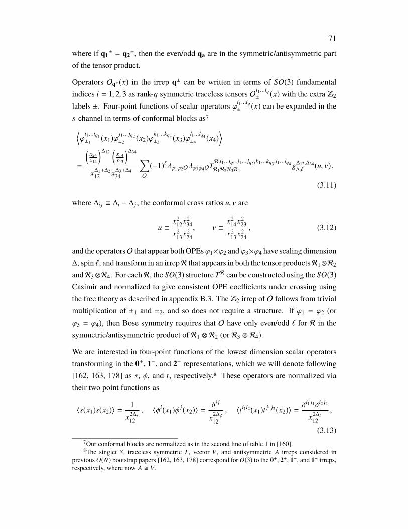
71

where if q1± = q2

±, then the even/odd qa are in the symmetric/antisymmetric partof the tensor product.

Operators Oq±(x) in the irrep q± can be written in terms of SO(3) fundamentalindices i = 1, 2, 3 as rank-q symmetric traceless tensors Oi1...iq

± (x) with the extra Z2

labels ±. Four-point functions of scalar operators ϕi1...iq± (x) can be expanded in the

s-channel in terms of conformal blocks as7⟨ϕ

i1...iq1±1 (x1)ϕ

j1... jq2±2 (x2)ϕ

k1...kq3±3 (x3)ϕ

l1...lq4±4 (x4)

⟩=

(x24x14

)∆12 (x14x13

)∆34

x∆1+∆212 x∆3+∆4

34

∑O

(−1)`λϕ1ϕ2Oλϕ3ϕ4OTR,i1...iq1, j1... jq2,k1...kq3,l1...lq4R1R2R3R4

g∆12,∆34∆,`

(u, v) ,

(3.11)

where ∆i j ≡ ∆i − ∆ j , the conformal cross ratios u, v are

u ≡x2

12x234

x213x2

24, v ≡

x214x2

23

x213x2

24, (3.12)

and the operatorsO that appear bothOPEs ϕ1×ϕ2 and ϕ3×ϕ4 have scaling dimension∆, spin `, and transform in an irrepR that appears in both the tensor productsR1⊗R2

and R3⊗R4. For each R, the SO(3) structureTR can be constructed using the SO(3)Casimir and normalized to give consistent OPE coefficients under crossing usingthe free theory as described in appendix B.3. The Z2 irrep of O follows from trivialmultiplication of ±1 and ±2, and so does not require a structure. If ϕ1 = ϕ2 (orϕ3 = ϕ4), then Bose symmetry requires that O have only even/odd ` for R in thesymmetric/antisymmetric product of R1 ⊗ R2 (or R3 ⊗ R4).

We are interested in four-point functions of the lowest dimension scalar operatorstransforming in the 0+, 1−, and 2+ representations, which we will denote following[162, 163, 178] as s, φ, and t, respectively.8 These operators are normalized viatheir two point functions as

〈s(x1)s(x2)〉 =1

x2∆s12

, 〈φi(x1)φj(x2)〉 =

δi j

x2∆φ12

, 〈ti1i2(x1)t j1 j2(x2)〉 =δi1 j1δi2 j2

x2∆t12

,

(3.13)7Our conformal blocks are normalized as in the second line of table 1 in [160].8The singlet S, traceless symmetric T , vector V , and antisymmetric A irreps considered in

previous O(N) bootstrap papers [162, 163, 178] correspond for O(3) to the 0+, 2+, 1−, and 1− irreps,respectively, where now A V .

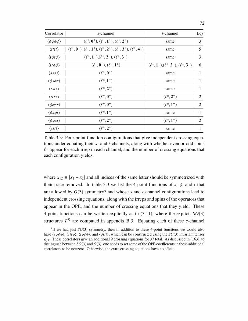
72

Correlator s-channel t-channel Eqs

〈φφφφ〉 (`+, 0+), (`−, 1+), (`+, 2+) same 3

〈tttt〉 (`+, 0+), (`−, 1+), (`+, 2+), (`−, 3+), (`+, 4+) same 5

〈tφtφ〉 (`±, 1−),(`±, 2−), (`±, 3−) same 3

〈ttφφ〉 (`+, 0+), (`−, 1+) (`±, 1−),(`±, 2−), (`±, 3−) 6

〈ssss〉 (`+, 0+) same 1

〈φsφs〉 (`±, 1−) same 1

〈tsts〉 (`±, 2+) same 1

〈ttss〉 (`+, 0+) (`±, 2+) 2

〈φφss〉 (`+, 0+) (`±, 1−) 2

〈φsφt〉 (`±, 1−) same 1

〈φφst〉 (`+, 2+) (`±, 1−) 2

〈sttt〉 (`±, 2+) same 1

Table 3.3: Four-point function configurations that give independent crossing equa-tions under equating their s- and t-channels, along with whether even or odd spins`± appear for each irrep in each channel, and the number of crossing equations thateach configuration yields.

where x12 ≡ |x1 − x2 | and all indices of the same letter should be symmetrized withtheir trace removed. In table 3.3 we list the 4-point functions of s, φ, and t thatare allowed by O(3) symmetry9 and whose s and t-channel configurations lead toindependent crossing equations, along with the irreps and spins of the operators thatappear in the OPE, and the number of crossing equations that they yield. These4-point functions can be written explicitly as in (3.11), where the explicit SO(3)structures TR are computed in appendix B.3. Equating each of these s-channel

9If we had just SO(3) symmetry, then in addition to these 4-point functions we would alsohave 〈sφφφ〉, 〈sttφ〉, 〈tφφφ〉, and 〈φttt〉, which can be constructed using the SO(3) invariant tensorεi jk . These correlators give an additional 9 crossing equations for 37 total. As discussed in [163], todistinguish between SO(3) andO(3), one needs to set some of the OPE coefficients in these additionalcorrelators to be nonzero. Otherwise, the extra crossing equations have no effect.

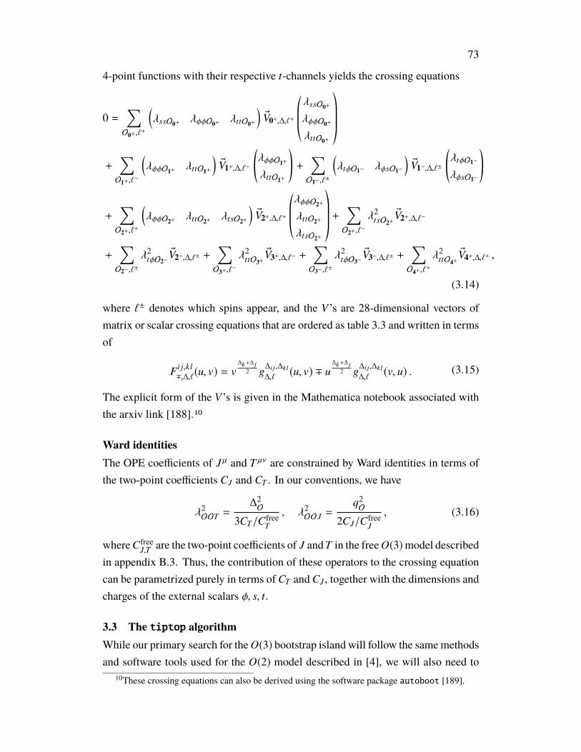
73

4-point functions with their respective t-channels yields the crossing equations

0 =∑O0+,`

+

(λssO0+ λφφO0+ λttO0+

)®V0+,∆,`+

©­­«λssO0+

λφφO0+

λttO0+

ª®®®¬+

∑O1+,`

−

(λφφO1+ λttO1+

)®V1+,∆,`−

(λφφO1+

λttO1+

)+

∑O1−,`±

(λtφO1− λφsO1−

)®V1−,∆,`±

(λtφO1−

λφsO1−

)

+∑O2+,`

+

(λφφO2+ λttO2+ λtsO2+

)®V2+,∆,`+

©­­«λφφO2+

λttO2+

λtsO2+

ª®®®¬ +∑O2+,`

−

λ2tsO2+®V2+,∆,`−

+∑O2−,`±

λ2tφO2−

®V2−,∆,`± +∑O3+,`

−

λ2ttO3+®V3+,∆,`− +

∑O3−,`±

λ2tφO3−

®V3−,∆,`± +∑O4+,`

+

λ2ttO4+®V4+,∆,`+ ,

(3.14)

where `± denotes which spins appear, and the V’s are 28-dimensional vectors ofmatrix or scalar crossing equations that are ordered as table 3.3 and written in termsof

Fi j,kl∓,∆,`(u, v) = v

∆k+∆j2 g

∆i j,∆kl∆,`

(u, v) ∓ u∆k+∆j

2 g∆i j,∆kl∆,`

(v, u) . (3.15)

The explicit form of the V’s is given in the Mathematica notebook associated withthe arxiv link [188].10

Ward identitiesThe OPE coefficients of Jµ and T µν are constrained by Ward identities in terms ofthe two-point coefficients CJ and CT . In our conventions, we have

λ2OOT =

∆2O

3CT/CfreeT

, λ2OOJ =

q2O

2CJ/CfreeJ

, (3.16)

whereCfreeJ,T are the two-point coefficients of J andT in the freeO(3)model described

in appendix B.3. Thus, the contribution of these operators to the crossing equationcan be parametrized purely in terms of CT and CJ , together with the dimensions andcharges of the external scalars φ, s, t.

3.3 The tiptop algorithmWhile our primary search for theO(3) bootstrap island will follow the samemethodsand software tools used for the O(2) model described in [4], we will also need to

10These crossing equations can also be derived using the software package autoboot [189].

74

compute the maximum value of the scaling dimension ∆t4 over this island. Thisemploys a new search strategy and software implementation that we describe in thissection.

Software and algorithmTo automate finding the maximally allowed value of some gap across the allowedregion, we have written tiptop, software for generating successive points forsearching for the maximum value of a coordinate achieved by a region in (N + 1)-dimensional space (see Appendix B.1). It has many optimizations specifically forfinding the maximum gap. It is meant to be invoked by a driver that takes thesepoints, computes whether they are feasible, and then asks for more points to check.

The number of dimensions is arbitrary but fixed at compile time. For concretenessand ease of visualization, we assume that N + 1 = 3 for the rest of this discussion,where the dimensions are ∆φ,∆s, and ∆gap. The algorithm operates unchanged forhigher dimensions.

We start with at least one feasible point, a cloud of infeasible points, a cloud ofpoints that are in-progress, and a maximum gap (∆max_gap). In-progress points arepoints that the driver already knows about and is working on, but does not yet knowif they are feasible. For example, those calculations may have been submitted ascalculations to an HPC cluster but not yet completed.

We assume that there are no feasible points with ∆gap ≥ ∆max_gap. We also assumethat islands only shrink at larger gaps. So if a point is infeasible at one gap, itwill continue to be infeasible at larger gaps. The last assumption is that each N-dimensional island at a fixed value of ∆gap is convex and simply connected, so eachisland never become a horseshoe or splits into two pieces. While there are manyexamples of islands splitting at low Λ, islands at high Λ have been well behaved fora wide variety of theories.

The basic outline of the algorithm for generating points is:

• Set ∆feasible to the largest ∆gap with a feasible point.

• Explore parameters at ∆feasible to find the size of the island there. If there areany corners of parameter space left to map out, return one point from there.(Section 3.3)

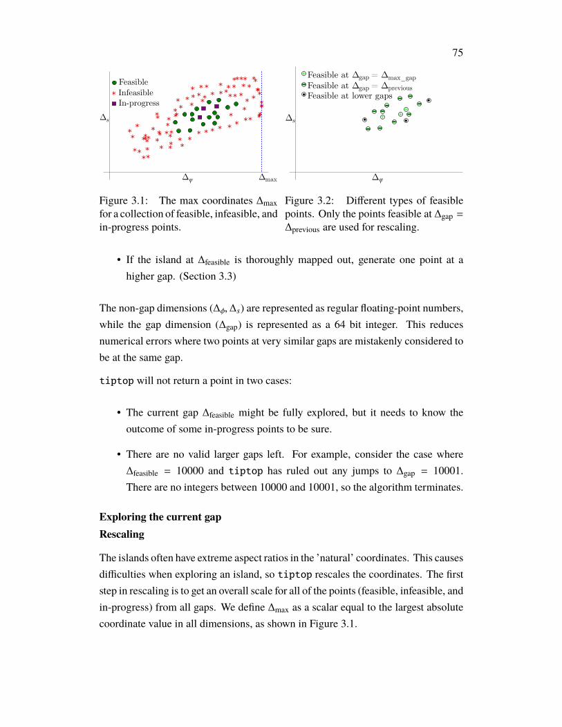
75

Feasible

* InfeasibleIn-progress

**

***

***

** * *

* *********

***

***

**** *

***

***

*

** * * *

* **

**

**

*******

** ****** *

*

* * *

***

** ****

*

Δφ

Δs

maxΔ

Figure 3.1: The max coordinates ∆maxfor a collection of feasible, infeasible, andin-progress points.

Δφ

Δs

Feasible at Δ = ΔgapFeasible at Δ = ΔgapFeasible at lower gaps

max_gap

previous

Figure 3.2: Different types of feasiblepoints. Only the points feasible at ∆gap =∆previous are used for rescaling.

• If the island at ∆feasible is thoroughly mapped out, generate one point at ahigher gap. (Section 3.3)

The non-gap dimensions (∆φ,∆s) are represented as regular floating-point numbers,while the gap dimension (∆gap) is represented as a 64 bit integer. This reducesnumerical errors where two points at very similar gaps are mistakenly considered tobe at the same gap.

tiptop will not return a point in two cases:

• The current gap ∆feasible might be fully explored, but it needs to know theoutcome of some in-progress points to be sure.

• There are no valid larger gaps left. For example, consider the case where∆feasible = 10000 and tiptop has ruled out any jumps to ∆gap = 10001.There are no integers between 10000 and 10001, so the algorithm terminates.

Exploring the current gapRescaling

The islands often have extreme aspect ratios in the ’natural’ coordinates. This causesdifficulties when exploring an island, so tiptop rescales the coordinates. The firststep in rescaling is to get an overall scale for all of the points (feasible, infeasible, andin-progress) from all gaps. We define ∆max as a scalar equal to the largest absolutecoordinate value in all dimensions, as shown in Figure 3.1.

76

For a given ∆max_gap, we define ∆previous as the largest gap with feasible points butless than ∆max_gap. This is usually a previous value for ∆max_gap. Figure 3.2 showsan example of feasible points at ∆max_gap, ∆previous, and lower gaps.

Using the m feasible points at ∆previous, we scale the points using a principle com-ponent analysis. Specifically, we construct the matrix

M =

©­­­­­­­­«

∆φ0 ∆s0

∆φ1 ∆s1

∆φ2 ∆s2

∆φ3 ∆s3...

...

ª®®®®®®®®¬.

We then compute the singular value decomposition (SVD) of this matrix

M = UΣV∗ , (3.17)

where Σ is a rectangular m × N diagonal matrix with non-negative real numbersσi = Σii on the diagonal ranging from the smallest (σmin) to the largest (σmax). U isan m × m unitary matrix, and V is an N × N (here 2 × 2) unitary matrix.

We define the N × N matrix Ω as the first N rows of Σ. This is a diagonal matrixwith the entries σi, so the inverse is trivial. Putting this all together, we define therescaling matrix

R ≡ σminΩ−1VT/(1.75 × ∆max) . (3.18)

It may be that there are so few points at∆previous that they are not linearly independent.For example, in the beginning, there may not be any points at ∆previous. If the ratiobetween the smallest (σmin) and largest (σmax) of these singular values is less thana tolerance (we use 10−8), then we only scale by ∆max

R ≡ I/(1.75 × ∆max) , (3.19)

where I is the identity.

Everything is scaled by the largest coordinate value ∆max to guarantee that all pointsare mapped into a box with extents (-1,1) in every dimension. The factor of 1.75(about

√3) is to ensure that all points will fit into the unit box even after rotation.

The transformation has the effect of a rotation and then rescaling of the rotatedcoordinates, so the feasible region remains convex. However, the feasible points

77

Feasible* InfeasibleIn-progress

**

***

*** * * * *

* ***********

******* * *

** ***

*

*

* * * **

* **

****

***

***

** ******* *

* * * ****

***

**** 1

1

-1

-1

Figure 3.3: Points from Figure3.1 after rescaling.

Feasible* Infeasible

In-progress

**

***

*** * * * *

* ***********

******* * *

** ***

*

*

* * * **

* **

****

***

***

** ******* *

* * * ****

***

****Candidate Cell

Figure 3.4: Points from Figure 3.3 with anadapted mesh. Points that are feasible at ∆gap <∆feasible have been removed. The blue spiral indi-cates an empty candidate cell. The other emptycells are not diagonal from a feasible cell, so theyare not considered.

should outline a more circular shape than the extended ellipse we started with, asshown in Figure 3.3.

One concern with this rescaling algorithm is that it weighs dense regions with morepoints more than equivalently sized regions with fewer points. So it may not producean optimal transform. In practice, the later steps spread out the points very evenly,so this concern turns out not to be a problem in practice.

Adaptively meshing the box

While the distribution of points in Figure 3.3 no longer has extreme aspect ratios,the points are still clustered in a small region of the unit box.

Based on the assumption that the feasible island only shrinks as the gap increases,we now only consider three sets of points: feasible at the current ∆max_gap, andinfeasible or in-progress at ∆gap ≤ ∆max_gap. For the rest of this step, we will betreating in-progress and infeasible points identically.

The strategy is to place points in regions that are empty. To quantify this emptiness,we create a regular mesh covering the points. Empty regions are then cells that haveno points. We start with a very coarse mesh consisting of a single cell covering theentire unit box. Then we loop over all cells, splitting each cell a point into 2N cells(4 for our example). We recursively loop over these new cells, continuing until wehave reached the minimum cell size.

78

The minimum cell size is set by multiplying the minimum coordinate extents ofthe rescaled feasible points by a fixed fraction fcutoff. In Figure 3.3, this minimumextent is about 0.5 in both dimensions. We use fcutoff = 2, which is deliberatelyvery coarse. If fcutoff < 1, then the algorithm will feel the need to completely fill ininternal regions, even though, by assumption, the internal spaces do not need to bechecked.

Just after a jump to a higher gap, there is only one feasible point at ∆feasible. Inthis case, the extents are zero, so we use a default minimum cell width of 2−47.This is quite small, but a little bigger than the minimum resolution of an IEEE-754double-precision number (2−53). This helps reduce errors from round-tripping thenumber through different systems.

Most of these cells will be empty. We select the largest empty cell that is adjacentto a cell containing only feasible points. If there are multiple empty cells next toa feasible cell, then we select a new cell in the order (+,+), (−,−), (+,−), (−,+) asin Figure 3.4. We only check diagonals, so points get laid out in a checkerboardpattern.

If there are two candidate empty cells, we choose the cell adjacent to the first feasiblepoint given to tiptop. So when driving tiptop, we always list the feasible pointsin the same order.

The new point is not placed at the center of the new cell, but rather simply offsetfrom the existing feasible point. So if the feasible point is in a corner of a cell, thenew point will be in the same corner of the empty cell.

The observed behavior of this algorithm is that it quickly finds a rough estimate forthe boundary between feasible and unfeasible, but can spend a lot of effort findingthe exact boundaries. In-progress points are treated as infeasible, so too manyin-progress points will lead to extra work. In practice, we have up to 16 pointsin-progress at any one time.

Jumping to a larger gapIf the previous section does not yield a new point, and there are no in-progresspoints, then we try to jump to a larger gap.

We start by rescaling the points as in section 3.3. We draw a coordinate box aroundall of the points feasible at ∆feasible and shrink it by a factor of 2. Then we find thelargest gap ∆ceiling that can accommodate this box without containing any infeasible

79

or in-progress points with ∆gap ≤ ∆ceiling. At the beginning, there are no infeasiblepoints at large gaps, so ∆ceiling = ∆max_gap.

We return the center of the box at ∆gap =(∆feasible + ∆ceiling

)/2, thus bisecting the

range of feasible gaps. This underscores the need for a good estimate of ∆max_gap.

If the estimate is too high, then the algorithm will recommend too many points thatare far too large.

Overall, we have found this approach to work reasonably well. More importantly, itis very robust. It is very easy to be too clever, resulting in odd failures.

3.4 ResultsDimension bounds with OPE scansNext we present our conformal bootstrap island computed using sdpb, along with itscomparison with various Monte Carlo results. Computing the conformal bootstrapisland requires scanning over the three operator dimensions ∆φ,∆s,∆t using theDelaunay search algorithm described in [4], and for each point using the "cuttingsurface" algorithm presented in [4] to decide if there exists an allowed point in thespace of OPE coefficient ratios sss

φφs, tts

φφs, φφtφφs, ttt

φφs.

When computing the island we make the following assumptions about the spectrumunless stated otherwise. We assume that φ, s, and t are the only relevant operatorsin their respective symmetry representations, so that ∆φ′,s′,t ′ ≥ 3. In addition, weassume that the leading rank-4 scalar has a dimension satisfying ∆t4 ≥ 2. Weassume an O(3) current with ∆J = 2 and stress tensor with ∆T = 3, with coefficientssatisfying the Ward identity constraints. We also impose a twist gap above them, aswell as in all other sectors not mentioned above, of size 10−6.

In Figure 3.5 we show the conformal bootstrap island we have computed at Λ = 43using these assumptions, compared to theMonte Carlo results of [7, 8]. In Figure 3.6we show various 2d projections of the bootstrap island. In appendix B.4 we givethe full set of allowed and disallowed points we computed at Λ = 43, along withFigure B.1 which shows the convergence of the allowed points as a function ofΛ after performing an affine transformation to make the allowed regions roughlyspherical.

In these plots we show our best determination of the allowed region at a given Λ,constructed by computing a Delaunay triangulation of the tested points, choosingtriangles that contain both allowed and disallowed points, and plotting the convex

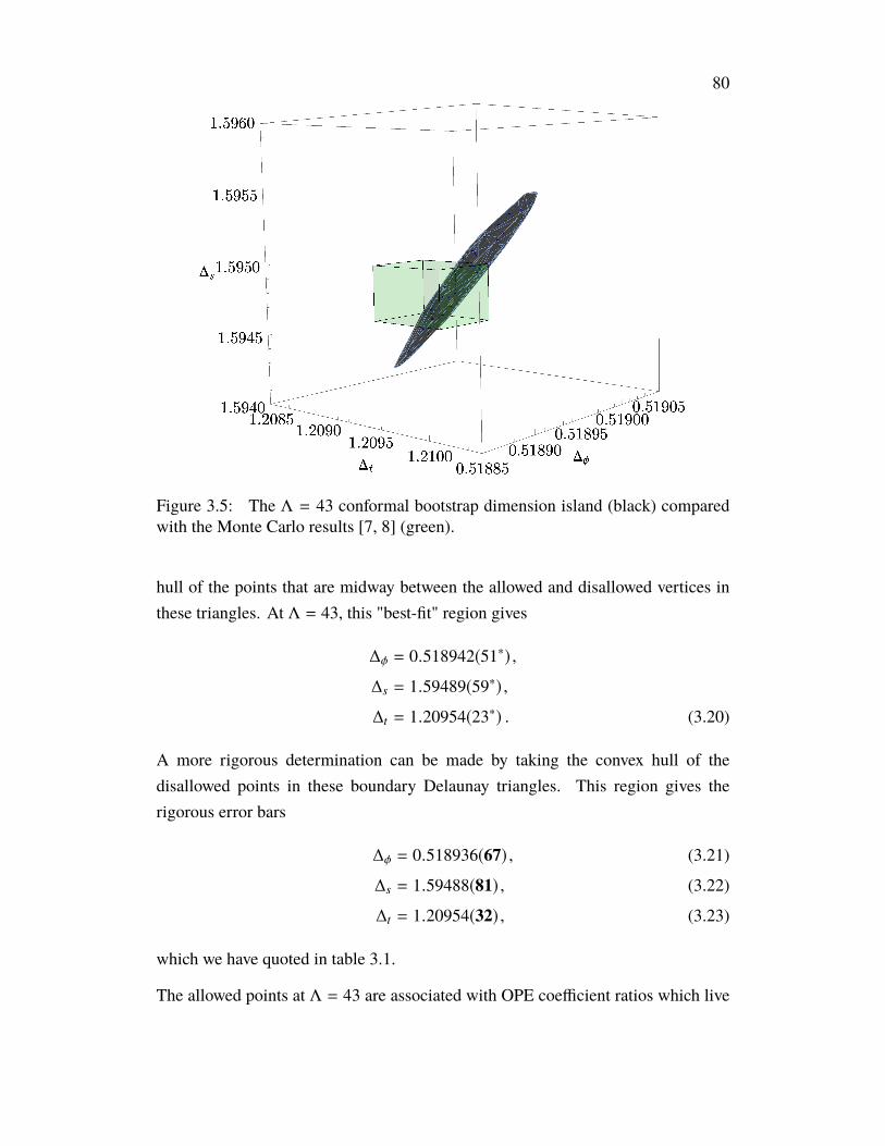
80

Figure 3.5: The Λ = 43 conformal bootstrap dimension island (black) comparedwith the Monte Carlo results [7, 8] (green).

hull of the points that are midway between the allowed and disallowed vertices inthese triangles. At Λ = 43, this "best-fit" region gives

∆φ = 0.518942(51∗) ,

∆s = 1.59489(59∗) ,

∆t = 1.20954(23∗) . (3.20)

A more rigorous determination can be made by taking the convex hull of thedisallowed points in these boundary Delaunay triangles. This region gives therigorous error bars

∆φ = 0.518936(67) , (3.21)

∆s = 1.59488(81) , (3.22)

∆t = 1.20954(32) , (3.23)

which we have quoted in table 3.1.

The allowed points at Λ = 43 are associated with OPE coefficient ratios which live

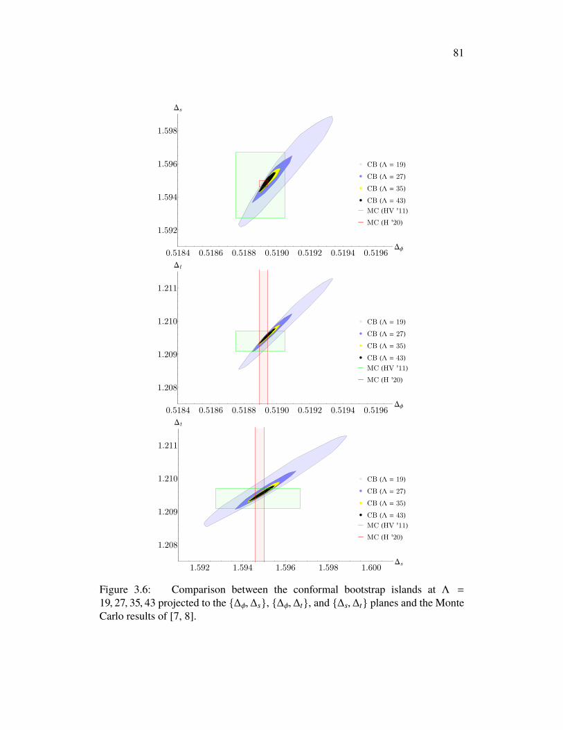
81

0.5184 0.5186 0.5188 0.5190 0.5192 0.5194 0.5196Δϕ

1.592

1.594

1.596

1.598

Δs

CB (Λ = 19)

CB (Λ = 27)

CB (Λ = 35)

CB (Λ = 43)MC (HV '11)

MC (H '20)

0.5184 0.5186 0.5188 0.5190 0.5192 0.5194 0.5196Δϕ

1.208

1.209

1.210

1.211

Δt

CB (Λ = 19)

CB (Λ = 27)

CB (Λ = 35)

CB (Λ = 43)MC (HV '11)

MC (H '20)

1.592 1.594 1.596 1.598 1.600Δs

1.208

1.209

1.210

1.211

Δt

CB (Λ = 19)

CB (Λ = 27)

CB (Λ = 35)

CB (Λ = 43)MC (HV '11)

MC (H '20)

Figure 3.6: Comparison between the conformal bootstrap islands at Λ =19, 27, 35, 43 projected to the ∆φ,∆s, ∆φ,∆t, and ∆s,∆t planes and the MonteCarlo results of [7, 8].

82

in the ranges11

λsss

λφφs= 0.9643(20∗) ,

λtts

λφφs= 1.87593(53∗) ,

λφφt

λφφs= 1.66808(23∗) ,

λttt

λφφs= 2.86034(61∗) . (3.24)

These should be viewed as an approximation to the full allowed region of OPEcoefficients, which may be slightly larger.

Central charges and λφφs

Next, we compute upper and lower bounds on the magnitude of the OPE coefficientλφφs, the central charge CT , and the current central charge CJ . We compute thesebounds over a small sample of points in our allowed region so the results will beinherently non-rigorous. However, we believe that this treatment gives reasonableestimates for these quantities that are more precise than previous results.

The strategy is similar to the method we employed in [4]. We take seven primalpoints in the Λ = 43 island, consisting of the scaling dimensions and allowed OPEcoefficients. The points are chosen to be sufficiently symmetrized and sparse acrossthe Λ = 43 island we have computed. For each of these points, we extremize CT ,CJ , and the external OPE norm parameterized by λφφs, to obtain upper and lowerbounds. This calculation was limited to Λ = 35 due to our available computationalresources. The data points and SDPB parameters we used are summarized in tablesB.5 and B.2, respectively.

There is an important comment wewant to make about the upper bound computationon CT and CJ (a similar comment was made in [4]). For computing upper boundson CT and CJ , we have to assume a gap ∆T ′/J ′ above the unitarity bound for the nextoperators in the T or J sectors. Note that this gap was not assumed in our OPE scan,so this extra constraint might turn an allowed point into a disallowed point. If we donot have such a gap, the upper bound is loose and may not give reasonable results.On the other hand, large gaps can make SDPB unable to find a solution.

11Note that there is an ambiguity in the signs of these coefficients, related to performing theoperator redefinitions s → −s and t → −t. This freedom can be used to fix λφφs and λφφt to bepositive, after which all other signs in (3.24) are determined to be positive by the conformal bootstrap.

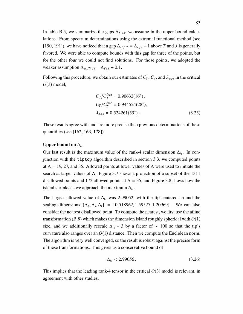
83

In table B.5, we summarize the gaps ∆T ′/J ′ we assume in the upper bound calcu-lations. From spectrum determinations using the extremal functional method (see[190, 191]), we have noticed that a gap ∆T ′/J ′ = ∆T/J + 1 above T and J is generallyfavored. We were able to compute bounds with this gap for three of the points, butfor the other four we could not find solutions. For those points, we adopted theweaker assumption ∆ext,T(J) = ∆T/J + 0.1.

Following this procedure, we obtain our estimates of CT , CJ , and λφφs in the criticalO(3) model,

CJ/CfreeJ = 0.90632(16∗) ,

CT/CfreeT = 0.944524(28∗) ,

λφφs = 0.524261(59∗) . (3.25)

These results agree with and are more precise than previous determinations of thesequantitites (see [162, 163, 178]).

Upper bound on ∆t4

Our last result is the maximum value of the rank-4 scalar dimension ∆t4 . In con-junction with the tiptop algorithm described in section 3.3, we computed pointsat Λ = 19, 27, and 35. Allowed points at lower values of Λ were used to initiate thesearch at larger values of Λ. Figure 3.7 shows a projection of a subset of the 1311disallowed points and 172 allowed points at Λ = 35, and Figure 3.8 shows how theisland shrinks as we approach the maximum ∆t4 .

The largest allowed value of ∆t4 was 2.99052, with the tip centered around thescaling dimensions ∆φ,∆s,∆t = 0.518962, 1.59527, 1.20969. We can alsoconsider the nearest disallowed point. To compute the nearest, we first use the affinetransformation (B.8) which makes the dimension island roughly spherical with O(1)size, and we additionally rescale ∆t4 − 3 by a factor of ∼ 100 so that the tip’scurvature also ranges over an O(1) distance. Then we compute the Euclidean norm.The algorithm is very well converged, so the result is robust against the precise formof these transformations. This gives us a conservative bound of

∆t4 < 2.99056 . (3.26)

This implies that the leading rank-4 tensor in the critical O(3) model is relevant, inagreement with other studies.

84

Figure 3.7: Two-dimensional projection of the results of the tiptop search at Λ =35. The x coordinate is related to the three scalar dimensions via (B.8). Projectionsin y and z look similar. We have superimposed a convex hull encompassing theallowed points on top, obscuring some of the disallowed points. We can see thebehaviour of the tiptop algorithm, exploring the island at one ∆t4 before jumpingto a larger ∆t4 . The jumps become progressively smaller, indicating convergence.We computed 16 points simultaneously, and this calculation took several monthsduring which the tiptop algorithm was being developed. So the points reflectoccasional crashes and small inefficiencies in the set of computed points.

3.5 Future directionsIn this workwe have applied themethods developed in [4, 5] for large-scale bootstrapproblems to the critical O(3) model in three dimensions. This has led to resultsfor scaling dimensions which are competitive with the most precise Monte Carlosimulations, and results for OPE coefficients which are significantly more precisethan previous determinations. In addition, we have computed a rigorous boundon the scaling dimension of the leading rank-4 tensor, showing that it is relevant.Thus, any O(3) system with cubic anisotropy should flow to the cubic fixed point(discussed in section 3.1) instead of the Heisenberg fixed point.

An interesting direction for future research will be the application of conformalperturbation theory to this flow. The cubic model can be reached by perturbingthe O(3) CFT with the operator X ≡

∑3i=1 tiiii

4 , which breaks O(3) symmetry to thediscrete symmetry Z3 o S3. From the O(3) point of view, this term is a certaincomponent of the O(3) rank-4 tensor with dimension ∆t4 ' 2.99. On the other hand,

85

Figure 3.8: Three-dimensional islands of allowed points at different ∆t4 at Λ = 35,demonstrating how the islands shrink as we approach the maximum ∆t4 . The x, y,and z coordinates are related to the three scalar dimensions via (B.8). The valuesfor ∆t4, from the largest region to smallest, are 2.989, 2.99025, and 2.9905, withsmaller values including all allowed points at larger values.

in the cubic fixed point conformal perturbation theory predicts ∆X ' 3.01. Becausethis term is marginally irrelevant with δ = ∆X − 3 ' 0.01, if we want to reach thecubic fixed point by aMonte Carlo simulation, the size of the lattice has to be aroundthe order of 21/δ, which is impractical to implement.

An alternative way to estimate the cubic CFT data is using conformal perturbationtheory. We start with the perturbed action S = SO(3) + g

∫d3xX . Using the

formalism in [192], one finds the beta function to be

βg = −δg −vol Sd−1

2λX X Xg

2. (3.27)

The dimension of an operator O at the cubic fixed point is then given at linear orderin δ by ∆O = ∆0 + 2δλOOX/λX X X , where ∆0 is the dimension of correspondingoperator in the O(3) CFT. Specifically one obtains ∆X = ∆0 + 2δ, which justifies theestimate ∆X ' 3.01.

86

The OPE coefficient λX X X is proportional to λt4t4t4 . Unfortunately, using the setupof the present paper, we don’t have access to λt4t4t4 . To access λt4t4t4 , one needsto bootstrap all four-point functions involving φ, s, t, t4, which is a concrete taskfor future research. Here we can estimate that the correction to ∆t in the cubicfixed-point is of order δ = 0.01. On the other hand, the corrections to ∆φ,∆s start atorder δ2 ' 0.0001 since λφφt4 = λsst4 = 0. Note that in this work the error bar for ∆t

is much smaller than δ. Therefore a careful study of the φ, s, t, t4 system shouldyield a solid prediction for the correction to ∆t in the cubic model.

Of course, it will also be interesting to understand how to isolate the cubic fixedpoint more directly using the conformal bootstrap, perhaps using a larger system ofcorrelators than was considered in [179, 181, 182]. One can also straightforwardlyapply the large-scale bootstrap techniques we have developed to other O(N)models,as well as to 3d CFTs with fermions (using the newly developed software [193]) orto study conserved currents [194–196]. Using these methods one can also continueexploring larger systems of correlators that may help us to isolate CFTs containinggauge fields, such as 3d QED [197, 198] and 4d QCD.

Now that we have precisely isolated the O(3) model, we are also in position todo a more detailed study of its low-twist trajectories of operators as a functionof spin, which can be compared to analytical calculations using the LorentzianInversion formula [37, 199], following the approach of [5, 200, 201]. Such analyticaltechniques can also be used to estimate the leading Regge intercepts and relatedLorentzian data of the O(3) model. In future work it will also be important tounderstand how to better incorporate insights from the analytical bootstrap, suchas our precise understanding of the large spin asymptotics, into making large-scalenumerical methods even more powerful.

Acknowledgments

We thank Yinchen He, Igor Klebanov, Filip Kos, Zhijin Li, João Penendones,Junchen Rong, Slava Rychkov, Andreas Stergiou, and Ettore Vicari for discussions.WL, JL, and DSD are supported by Simons Foundation grant 488657 (SimonsCollaboration on the Nonperturbative Bootstrap). DSD and JL are also supportedby a DOE Early Career Award under grant no. DE-SC0019085. DP is supported

87

by Simons Foundation grant 488651 (Simons Collaboration on the Nonperturba-tive Bootstrap) and DOE grants DE-SC0020318 and DE-SC0017660. This projecthas received funding from the European Research Council (ERC) under the Euro-pean Union’s Horizon 2020 research and innovation programme (grant agreementno. 758903). AV is also supported by the Swiss National Science Foundation(SNSF) under grant no. PP00P2-163670. SMC is supported by a Zuckerman STEMLeadership Fellowship.

This work used the Extreme Science and Engineering Discovery Environment(XSEDE) Comet Cluster at the San Diego Supercomputing Center (SDSC) throughallocation PHY190023, which is supported by National Science Foundation grantnumber ACI-1548562. This work also used the EPFL SCITAS cluster, which issupported by the SNSF grant PP00P2-163670, the Caltech High Performance Clus-ter, partially supported by a grant from the Gordon and Betty Moore Foundation,and the Grace computing cluster, supported by the facilities and staff of the YaleUniversity Faculty of Sciences High Performance Computing Center.

88

C h a p t e r 4

COLLISIONS OF FALSE-VACUUM BUBBLE WALLS IN AQUANTUM SPIN CHAIN

This chapter is based on A. Milsted, J. Liu, J. Preskill and G. Vidal, Collisions offalse-vacuum bubble walls in a quantum spin chain, arXiv: 2012.07243 [quant-ph].

Abstract: We study the real-time dynamics of a small bubble of "false vacuum” ina quantum spin chain near criticality, where the low-energy physics is described bya relativistic (1+1)-dimensional quantum field theory. Such a bubble can be thoughtof as a confined kink-antikink pair (a meson). We carefully construct bubbles sothat particle production does not occur until the walls collide. To achieve this inthe presence of strong correlations, we extend a Matrix Product State (MPS) ansatzfor quasiparticle wavepackets [Van Damme et al., arXiv:1907.02474 (2019)] to thecase of confined, topological quasiparticles. By choosing the wavepacket width andthe bubble size appropriately, we avoid strong lattice effects and observe relativistickink-antikink collisions. We use the MPS quasiparticle ansatz to detect scatteringoutcomes: In the Ising model, with transverse and longitudinal fields, we do notobserve particle production despite nonintegrability (supporting recent observationsof nonthermalizing mesonic states). With additional interactions, we see productionof confined and unconfined particle pairs. Although we simulated these low-energy,few-particle events withmoderate resources, we observe significant growth of entan-glement with energy and with the number of collisions, suggesting that increasingeither will ultimately exhaust our methods. Quantum devices, in contrast, are notlimited by entanglement production, and promise to allow us to go far beyond clas-sical methods. We anticipate that kink-antikink scattering in 1+1 dimensions willbe an instructive benchmark problem for relatively near-term quantum devices.

It is possible that the known universe is built on top of a metastable, or "false”vacuum state. In this scenario, there is a small but nonzero probability of a smallbubble of "true” vacuum forming via tunneling, whose interior has a lower energydensity. Thus the bubble expands, its walls accelerating, bulldozing everythingin their path. If multiple bubbles of true vacuum form far apart, their walls willrush toward each other and eventually collide, producing showers of particles. Itis possible that such events have already occurred, and are thus relevant for the

89

evolution of the early universe [202–206]. Simulations could provide an importantwindow into these high-energy, strongly-coupled dynamical processes.

However, one does not easily simulate the dynamics of a strongly interacting quan-tum field theory (QFT), at least using classical computers. Quantum Monte Carlo– the workhorse for simulations of equilibrium phenomena in lattice systems (suchas lattice QCD [1]) – suffers from the sign problem that blocks its application toreal-time dynamics. Tensor-network methods show promise, and have been usedto simulate nontrivial dynamical phenomena in (1+1)D systems, such as stringbreaking in lattice gauge theory [207–212]. Nevertheless, the computational costincreases exponentially with time in the general case (due to linear scaling of entan-glement entropy) and also dramatically with the number of spatial dimensions.

In principle, quantum computers (both analog and digital) can simulate dynam-ics of quantum field theories at long timescales with polynomial costs [27, 28], atopic which has recently attracted great interest [23, 213–220, 220–233]. How-ever, existing or near-term digital quantum devices are noisy, such that only shallowquantum circuits can avoid being overwhelmed by errors. Analog quantum simu-lators can support longer coherence times but are typically limited to a small setof Hamiltonians and initial states. As such, for the time being, we expect classicalsimulations of physical systems to perform better, with quantum devices catchingup as the hardware improves, ultimately beating classical computers by an exponen-tial margin. Thus dynamical simulations of phenomena like false-vacuum collapseare physically-motivated applications for quantum computers and analog quantumsimulators, and can be used as benchmark problems as quantum devices improve.

In this paper, we develop a framework for simulating the full quantum dynamicsof false-vacuum bubble-wall collisions in (1+1) dimensions using Matrix ProductStates [234, 235], demonstrating the production of new particles (see Fig. 4.1). Notethat, in (1+1) dimensions, a false-vacuum bubble can be viewed as an excitedmesonstate consisting of a kink-antikink pair, where the kink and antikink are localized,spatially separated topological particles. The false vacuum plays the role of alow-energy string that binds the kink to the antikink (confinement). Furthermore,metastability of the false vacuum corresponds to suppression of string breaking[236]. We simulate the relaxation of such mesonic states, which we simply call"bubbles”, in which both the kink and antikink are of low mass. During relaxation,the kink and antikink will collide. This can be thought of as a scattering event, hencefalling into one of three categories: free (no interaction), elastic (interaction, but no

90

⟨𝑍⟩

𝑥

𝑡 ?(a)

(b)

(c)

Figure 4.1: Cartoon showing the collapse of a false-vacuum bubble in a spinchain. The magnetization 〈Z〉 is positive in the true vacuum, but negative in thefalse vacuum. A bubble-wall collision is a scattering process, which may be (a)free (no interaction), (b) elastic (no particle production), or (c) inelastic (particleproduction). Note that in free and elastic scattering of topological particles the left(right) particle always remains a kink (antikink).

particle production), and inelastic (particle production). We successfully simulateinelastic kink-antikink collisions over∼ 1000 lattice sites at energies of up to∼ 5mµ,where mµ is the mass of the lightest meson. We characterize scattering outcomes inour simulations by tracking the energy density and entanglement entropy, as well asby projecting the quantum state into different particle "sectors”.

Previous work on related phenomena includes MPS simulations of meson decay inthe Schwinger model [208–212, 237], where the initial state is typically preparedby applying a bare string operator to the vacuum. This generally creates multiplehighly-localized particles of varying energy at the string edges, leading to relativelycomplex dynamics. The rapid resulting entanglement growth can make it difficultto reach long times and to treat large systems. Such strings can be smeared out intowavepackets (as considered, for example in some recent work onmesonic excitationsin spin chains [231, 238]), which focuses the wavepacket momenta, significantlyreducing the energy and entanglement growth. Nevertheless, the smeared string willstill generally create multiple species of topological excitation. Recently, however,techniques have been developed [239] to construct wavepacket states with selectiveparticle content in generic (1+1)-dimensional systems using MPS 1. A main resultof our paper is that we can extend those techniques to build quasistable initial bubblestates which, aside from the acceleration of the walls under the confining force, donot change significantly until the walls collide. We achieve this by selecting a single

1Also see [240] for a Bethe-ansatz approach.

91

species of kink and antikink quasiparticle for the bubble-wall wavepackets, togetherwith the metastable false vacuum for the interior. Apart from further reducingthe energy and the rate of entanglement growth, which enables us to treat largersystems and simulate for longer times, this greatly improves the interpretability ofour simulations, since the only scattering events that occur come from bubble-wallcollisions. We contrast this with the smeared bare string construction, in whichmeson pairs are generally observed immediately, at the initial bubble walls, asshown in Fig. 4.2.

One approach to simulating the dynamics of QFT phenomena on the lattice is tospatially discretize a chosen QFT Hamiltonian [2, 28, 207–212, 241]. In many casesinvolving bosonic fields, however, this results in an infinite-dimensional Hilbertspace for each lattice site that must then be truncated. In this study, we considera quantum spin chain, chosen and tuned so that its low-energy physics is governedby an emergent relativistic QFT. This is known to occur in the vicinity of manycontinuous phase transitions, where the emergent QFT is often a (by definitionrelativistic) conformal field theory (CFT) (see e.g. [242]).

To summarize, partially motivated by a potential connection with early universecosmology, we have studied inelastic particle production arising from collisionsof confined kink-antikink pairs in a relativistic scalar field theory. We probe thequantum field theory by tuning close to a critical point of the spin chain describedin Sec. 4.1, ensuring that the kink and antikink lattice velocities remain below theirmaximum values, thus avoiding strong lattice artifacts. Our classical simulationsuse MPS approximations to the evolving quantum state, which are computationallyfeasible as long as the state does not become too highly entangled. By highlight-ing the limitations of such classical methods, our work clarifies where quantumadvantage might potentially arise in relatively near-term quantum simulators.

The initial state preparation for our dynamical simulations is subtle, because thekink-antikink pair is not an energy eigenstate. As discussed in Sec. 4.2, we takecare to prepare initial kink and antikink wavepackets which are broad comparedto the lattice spacing, and not contaminated by additional unwanted excitations.We also develop tools for analysis of the outgoing particles produced in inelastickink-antikink collisions. We show in Sec. 4.3 that particle production is stronglysuppressed in the Ising model with intrinsic Z2 symmetry breaking, even though themodel is nonintegrable in that case, and we show that copious particle productionoccurs once a Z2-symmetric three-site local interaction turns on. We also quan-

92

0 250 500 750position

100200300400500

time

(a) bare string, smeared

0 250 500 750position

(b) quasiparticle packets

6

5

4

3

2

log(

|e/E

|)

Figure 4.2: Evolution of the excess energy density e (relative to vacuum), as afraction of total excess energy E , in a spin chain for two initial states: (a) createdby applying a spatially smeared string operator to the vacuum and (b) constructedfrom MPS tensors to contain kink and antikink quasiparticle wavepackets. In (a)meson pairs are produced immediately at the string edges, whereas in (b) there isno particle production until the initial kink and antikink collide. The dynamics arerestricted to a window of ∼ 1000 sites, leading to boundary effects in (a). For moredetails, see App. C.6.

titatively track the growth of entanglement entropy during repeated kink-antikinkcollisions, thus inferring how large a bond dimension is needed to provide an accurateapproximation to the evolving quantum state. Sec. 4.4 contains concluding remarks,and further details of our methods and results are provided in the appendices.

4.1 Selecting a spin chainWe seek a spin chain whose IR physics is described by a relativistic emergent fieldtheory supporting confined kinks. In principle, there are many suitable models: Anemergent field theory of confined kink-antikink pairs can be engineered by startingwith a spontaneously-broken discrete symmetry, which provides multiple vacua andtopological excitations. We then tune close to a symmetry-breaking phase transition,typically described by a CFT, and finally add a weak symmetry-breaking field to liftthe vacuum degeneracy and confine the kinks. We must take care, however, sinceemergent field theories of such spin chains are sometimes integrable [243–246], inwhich case scattering, including kink collision, is elastic. If we want to observeparticle production in the emergent field theory, we must avoid integrability.

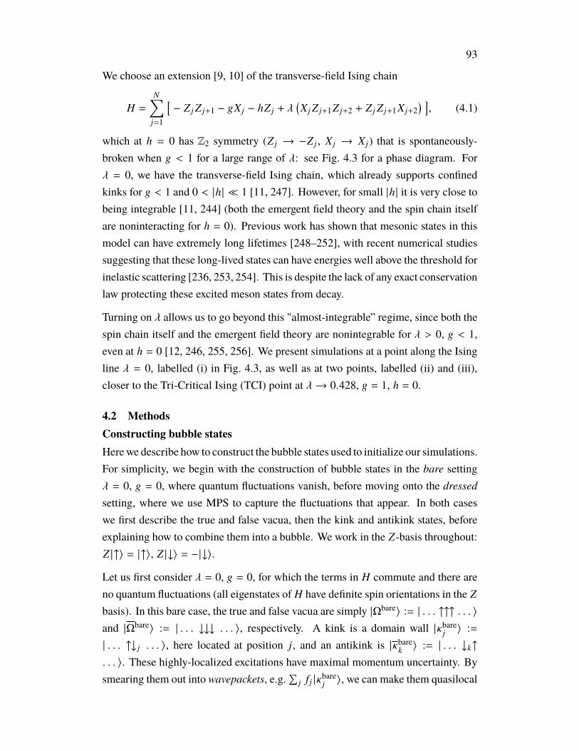
93

We choose an extension [9, 10] of the transverse-field Ising chain

H =N∑

j=1

[− Z j Z j+1 − gX j − hZ j + λ

(X j Z j+1Z j+2 + Z j Z j+1X j+2

) ], (4.1)

which at h = 0 has Z2 symmetry (Z j → −Z j , X j → X j) that is spontaneously-broken when g < 1 for a large range of λ: see Fig. 4.3 for a phase diagram. Forλ = 0, we have the transverse-field Ising chain, which already supports confinedkinks for g < 1 and 0 < |h| 1 [11, 247]. However, for small |h| it is very close tobeing integrable [11, 244] (both the emergent field theory and the spin chain itselfare noninteracting for h = 0). Previous work has shown that mesonic states in thismodel can have extremely long lifetimes [248–252], with recent numerical studiessuggesting that these long-lived states can have energies well above the threshold forinelastic scattering [236, 253, 254]. This is despite the lack of any exact conservationlaw protecting these excited meson states from decay.

Turning on λ allows us to go beyond this "almost-integrable” regime, since both thespin chain itself and the emergent field theory are nonintegrable for λ > 0, g < 1,even at h = 0 [12, 246, 255, 256]. We present simulations at a point along the Isingline λ = 0, labelled (i) in Fig. 4.3, as well as at two points, labelled (ii) and (iii),closer to the Tri-Critical Ising (TCI) point at λ→ 0.428, g = 1, h = 0.

4.2 MethodsConstructing bubble statesHerewe describe how to construct the bubble states used to initialize our simulations.For simplicity, we begin with the construction of bubble states in the bare settingλ = 0, g = 0, where quantum fluctuations vanish, before moving onto the dressedsetting, where we use MPS to capture the fluctuations that appear. In both caseswe first describe the true and false vacua, then the kink and antikink states, beforeexplaining how to combine them into a bubble. We work in the Z-basis throughout:Z |↑〉 = |↑〉, Z |↓〉 = −|↓〉.

Let us first consider λ = 0, g = 0, for which the terms in H commute and there areno quantum fluctuations (all eigenstates of H have definite spin orientations in the Z

basis). In this bare case, the true and false vacua are simply |Ωbare〉 := | . . . ↑↑↑ . . . 〉and |Ωbare〉 := | . . . ↓↓↓ . . . 〉, respectively. A kink is a domain wall |κbarej 〉 :=| . . . ↑↓ j . . . 〉, here located at position j, and an antikink is |κbarek 〉 := | . . . ↓k↑

. . . 〉. These highly-localized excitations have maximal momentum uncertainty. Bysmearing them out into wavepackets, e.g.

∑j f j |κ

barej 〉, we can make them quasilocal

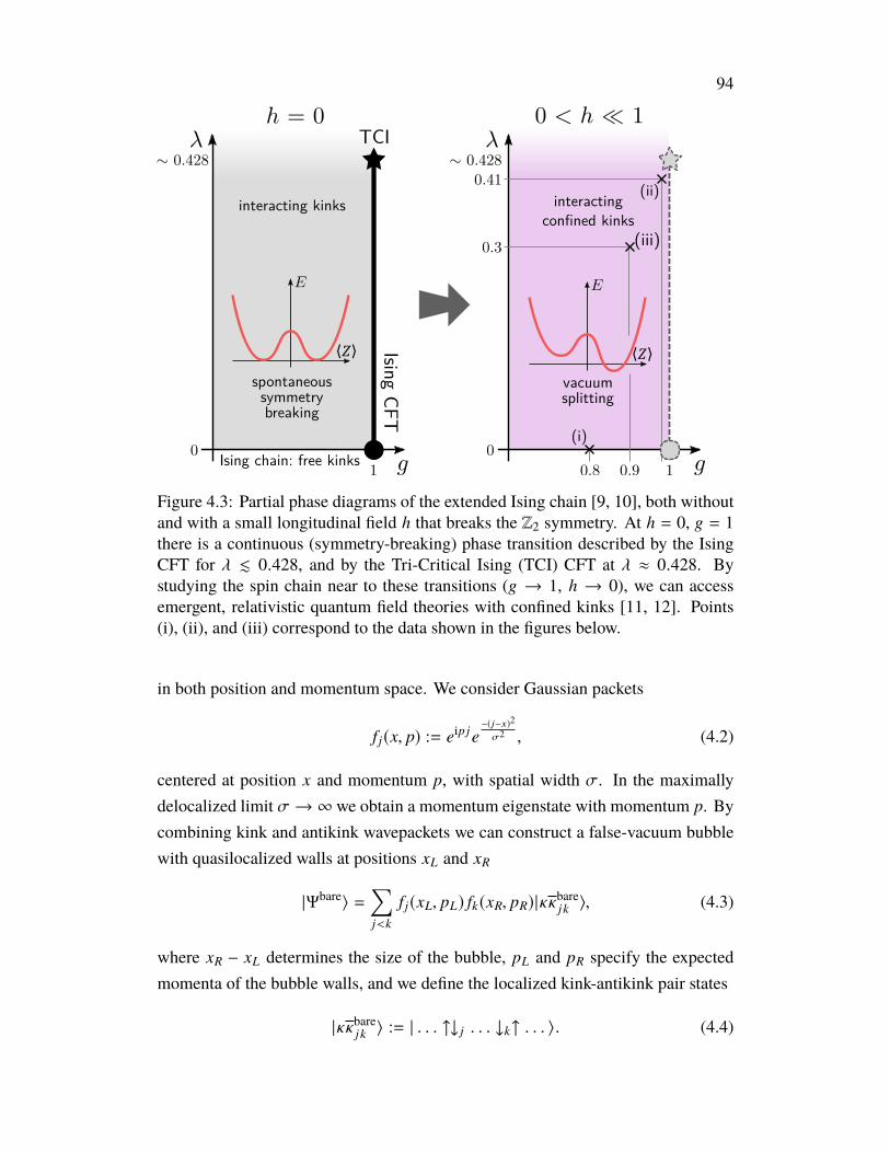
94

TCI

IsingCFT

Ising chain: free kinks

𝜆

𝑔

∼ 0.428

1

0

ℎ = 0𝜆

𝑔

∼ 0.428

1

0

0 < ℎ ≪ 1

spontaneoussymmetrybreaking

𝐸

⟨𝑍⟩

vacuumsplitting

𝐸

⟨𝑍⟩

interacting kinks interactingconfined kinks

0.3

0.8

(iii)

(i)

0.9

(ii)0.41

Figure 4.3: Partial phase diagrams of the extended Ising chain [9, 10], both withoutand with a small longitudinal field h that breaks the Z2 symmetry. At h = 0, g = 1there is a continuous (symmetry-breaking) phase transition described by the IsingCFT for λ . 0.428, and by the Tri-Critical Ising (TCI) CFT at λ ≈ 0.428. Bystudying the spin chain near to these transitions (g → 1, h → 0), we can accessemergent, relativistic quantum field theories with confined kinks [11, 12]. Points(i), (ii), and (iii) correspond to the data shown in the figures below.

in both position and momentum space. We consider Gaussian packets

f j(x, p) := eipje−(j−x)2

σ2 , (4.2)

centered at position x and momentum p, with spatial width σ. In the maximallydelocalized limit σ →∞ we obtain a momentum eigenstate with momentum p. Bycombining kink and antikink wavepackets we can construct a false-vacuum bubblewith quasilocalized walls at positions xL and xR

|Ψbare〉 =∑j<k

f j(xL, pL) fk(xR, pR)|κκbarej k 〉, (4.3)

where xR − xL determines the size of the bubble, pL and pR specify the expectedmomenta of the bubble walls, and we define the localized kink-antikink pair states

|κκbarej k 〉 := | . . . ↑↓ j . . . ↓k↑ . . . 〉. (4.4)

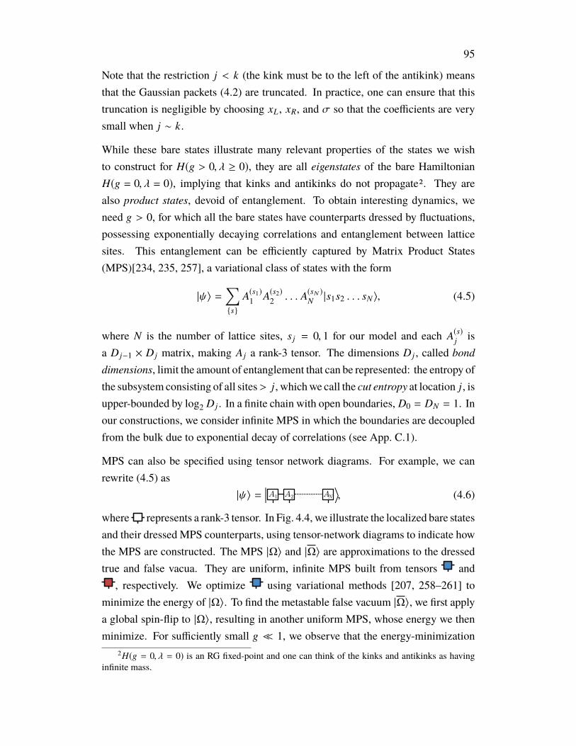
95

Note that the restriction j < k (the kink must be to the left of the antikink) meansthat the Gaussian packets (4.2) are truncated. In practice, one can ensure that thistruncation is negligible by choosing xL , xR, and σ so that the coefficients are verysmall when j ∼ k.

While these bare states illustrate many relevant properties of the states we wishto construct for H(g > 0, λ ≥ 0), they are all eigenstates of the bare HamiltonianH(g = 0, λ = 0), implying that kinks and antikinks do not propagate2. They arealso product states, devoid of entanglement. To obtain interesting dynamics, weneed g > 0, for which all the bare states have counterparts dressed by fluctuations,possessing exponentially decaying correlations and entanglement between latticesites. This entanglement can be efficiently captured by Matrix Product States(MPS)[234, 235, 257], a variational class of states with the form

|ψ〉 =∑s

A(s1)1 A(s2)

2 . . . A(sN )N |s1s2 . . . sN〉, (4.5)

where N is the number of lattice sites, s j = 0, 1 for our model and each A(s)j isa D j−1 × D j matrix, making A j a rank-3 tensor. The dimensions D j , called bonddimensions, limit the amount of entanglement that can be represented: the entropy ofthe subsystem consisting of all sites> j, whichwe call the cut entropy at location j, isupper-bounded by log2 D j . In a finite chain with open boundaries, D0 = DN = 1. Inour constructions, we consider infinite MPS in which the boundaries are decoupledfrom the bulk due to exponential decay of correlations (see App. C.1).

MPS can also be specified using tensor network diagrams. For example, we canrewrite (4.5) as

|ψ〉 = | ⟩𝐴1 𝐴2 𝐴𝑁 , (4.6)

where represents a rank-3 tensor. In Fig. 4.4, we illustrate the localized bare statesand their dressed MPS counterparts, using tensor-network diagrams to indicate howthe MPS are constructed. The MPS |Ω〉 and |Ω〉 are approximations to the dressedtrue and false vacua. They are uniform, infinite MPS built from tensors and

, respectively. We optimize using variational methods [207, 258–261] tominimize the energy of |Ω〉. To find the metastable false vacuum |Ω〉, we first applya global spin-flip to |Ω〉, resulting in another uniform MPS, whose energy we thenminimize. For sufficiently small g 1, we observe that the energy-minimization

2H(g = 0, λ = 0) is an RG fixed-point and one can think of the kinks and antikinks as havinginfinite mass.

96

|↑↑↑↓↓↓↓⟩

⟨𝑍⟩ ⟨𝑍⟩

| ⟩

⟨𝑍⟩

| ⟩ |↑↓↓↓↓↓↑⟩

⟨𝑍⟩

kink kink-antikink pair

|↑↑↑↑↑↑↑⟩

⟨𝑍⟩ ⟨𝑍⟩

| ⟩ |↓↓↓↓↓↓↓⟩

⟨𝑍⟩⟨𝑍⟩

| ⟩

⟨𝑍⟩

| ⟩|↑↑↑↓↑↑↑⟩

⟨𝑍⟩

vacuum

⟨𝑍⟩

| ⟩ |↑↓↑↑↑↓↑⟩

⟨𝑍⟩

meson meson pair

false vacuum|Ω⟩

|𝜅𝑗⟩

𝑗 𝑗 𝑘

|Ω⟩

matrix product statesproduct states product states

dressedbare bare

|Ωbare⟩ |Ωbare⟩

𝑗|𝜅bare⟩ 𝑗𝑘|𝜅𝜅bare⟩

𝑗 𝑗 𝑘

|𝜅𝜅𝑗𝑘⟩

|𝜇𝑗⟩ |𝜇𝜇𝑗𝑘⟩𝑗|𝜇bare⟩

Figure 4.4: Diagram illustrating the various types of states, and their spin profiles,relevant for simulations. For example, our initial states are wavepackets constructedfrom kink-antikink pairs (a type of excited meson). The product states listed areeigenstates of H when g = 0, λ = 0. Away from this regime, we use MPS toaccurately capture fluctuations in the vacua and excited states.

procedure does not find a path to the true ground state, resulting in a metastablefalse vacuum state |Ω〉, with MPS tensor , that behaves as an energy eigenstatefor all practical purposes (up to numerical precision – see App. C.2).

The MPS |κ j〉 approximates a dressed, localized kink state. It is constructed byintroducing a new tensor that sits at position j, between two semi-infinite chains,one consisting of on the left and one of on the right. The tensorparameterizes the spatial transition between the true and false vacuum regions.Unlike in the bare case, the transition region may encompass many lattice sites, asillustrated by the 〈Z〉 plots in Fig. 4.4. The antikink |κk〉 is similarly constructedby introducing a tensor between a chain of on the left and on the right.We select and using an MPS Bloch-state approach [235, 259, 260, 262]so that |κ j〉 and |κk〉 states can be thought of as "position bases” for the kinkand antikink quasiparticles of lowest energy. We use these states to constructtopological quasiparticle wavepackets

∑j f j |κ j〉 and

∑k fk |κk〉 [239]. If D is the

bond dimension of the vacuum MPS, such wavepackets have MPS representationswith bond dimension 2D (see App. C.3 for details).

The Bloch-state approach for finding and is conceptually simpler when h = 0,so that there is no confining force acting on the kinks and antikinks. We consider theh , 0 case further below. For h = 0, we solve an effectiveHamiltonian for and

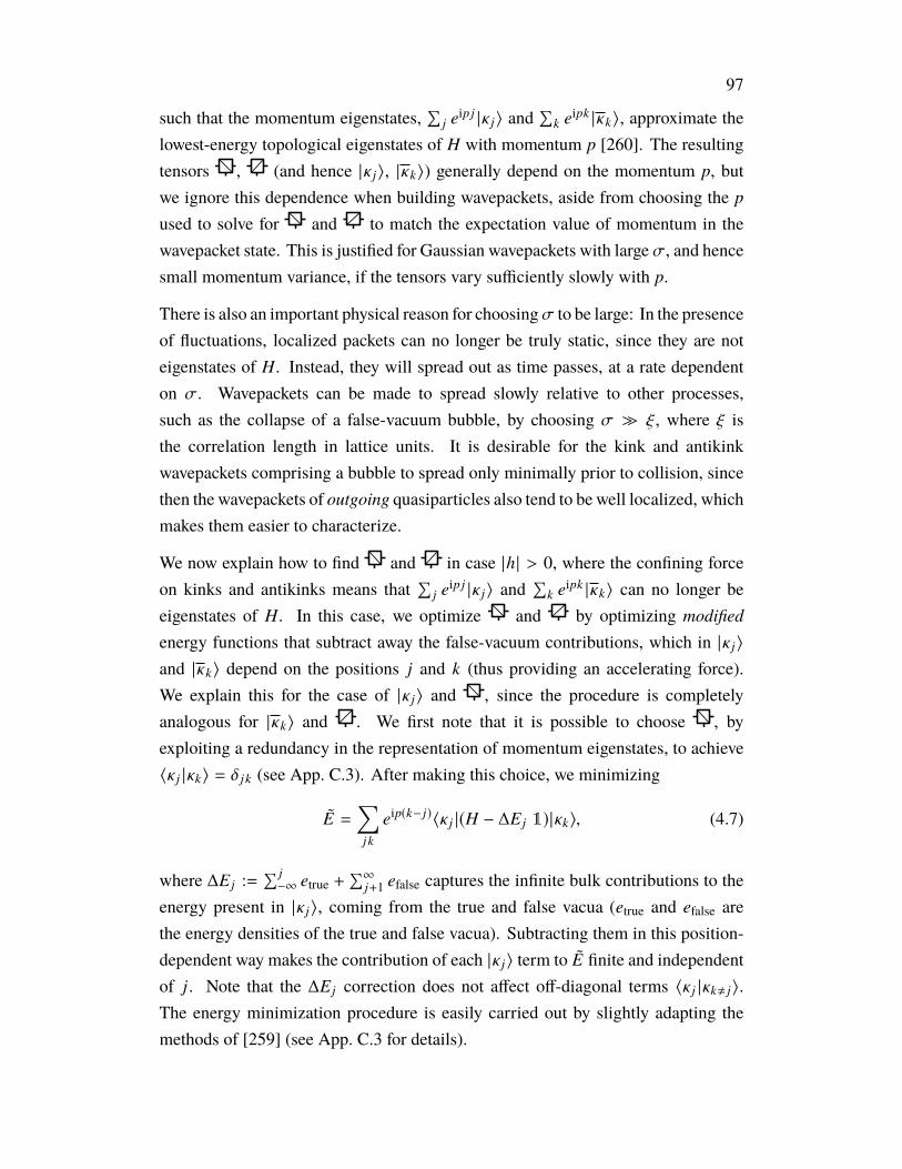
97

such that the momentum eigenstates,∑

j eipj |κ j〉 and∑

k eipk |κk〉, approximate thelowest-energy topological eigenstates of H with momentum p [260]. The resultingtensors , (and hence |κ j〉, |κk〉) generally depend on the momentum p, butwe ignore this dependence when building wavepackets, aside from choosing the p

used to solve for and to match the expectation value of momentum in thewavepacket state. This is justified for Gaussian wavepackets with large σ, and hencesmall momentum variance, if the tensors vary sufficiently slowly with p.

There is also an important physical reason for choosingσ to be large: In the presenceof fluctuations, localized packets can no longer be truly static, since they are noteigenstates of H. Instead, they will spread out as time passes, at a rate dependenton σ. Wavepackets can be made to spread slowly relative to other processes,such as the collapse of a false-vacuum bubble, by choosing σ ξ, where ξ isthe correlation length in lattice units. It is desirable for the kink and antikinkwavepackets comprising a bubble to spread only minimally prior to collision, sincethen the wavepackets of outgoing quasiparticles also tend to be well localized, whichmakes them easier to characterize.

We now explain how to find and in case |h| > 0, where the confining forceon kinks and antikinks means that

∑j eipj |κ j〉 and

∑k eipk |κk〉 can no longer be

eigenstates of H. In this case, we optimize and by optimizing modifiedenergy functions that subtract away the false-vacuum contributions, which in |κ j〉

and |κk〉 depend on the positions j and k (thus providing an accelerating force).We explain this for the case of |κ j〉 and , since the procedure is completelyanalogous for |κk〉 and . We first note that it is possible to choose , byexploiting a redundancy in the representation of momentum eigenstates, to achieve〈κ j |κk〉 = δ j k (see App. C.3). After making this choice, we minimizing

E =∑

j k

eip(k− j)〈κ j |(H − ∆E j 1)|κk〉, (4.7)

where ∆E j :=∑ j−∞ etrue +

∑∞j+1 efalse captures the infinite bulk contributions to the

energy present in |κ j〉, coming from the true and false vacua (etrue and efalse arethe energy densities of the true and false vacua). Subtracting them in this position-dependent way makes the contribution of each |κ j〉 term to E finite and independentof j. Note that the ∆E j correction does not affect off-diagonal terms 〈κ j |κk, j〉.The energy minimization procedure is easily carried out by slightly adapting themethods of [259] (see App. C.3 for details).

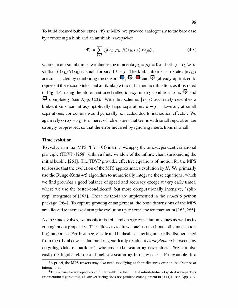
98

To build dressed bubble states |Ψ〉 as MPS, we proceed analogously to the bare caseby combining a kink and an antikink wavepacket

|Ψ〉 =∑j<k

f j(xL, pL) fk(xR, pR)|κκ j k〉 , (4.8)

where, in our simulations, we choose themomenta pL = pR = 0 and set xR−xL σ

so that f j(xL) fk(xR) is small for small k − j. The kink-antikink pair states |κκ j k〉

are constructed by combining the tensors , , and (already optimized torepresent the vacua, kinks, and antikinks) without further modification, as illustratedin Fig. 4.4, using the aforementioned reflection-symmetry condition to fix and

completely (see App. C.3). With this scheme, |κκ j k〉 accurately describes akink-antikink pair at asymptotically large separations k − j. However, at smallseparations, corrections would generally be needed due to interaction effects3. Weagain rely on xR − xL σ here, which ensures that terms with small separation arestrongly suppressed, so that the error incurred by ignoring interactions is small.

Time evolutionTo evolve an initial MPS |Ψ(t = 0)〉 in time, we apply the time-dependent variationalprinciple (TDVP) [258] within a finite window of the infinite chain surrounding theinitial bubble [261]. The TDVP provides effective equations of motion for the MPStensors so that the evolution of the MPS approximates evolution by H. We primarilyuse the Runge-Kutta 4/5 algorithm to numerically integrate these equations, whichwe find provides a good balance of speed and accuracy except at very early times,where we use the better-conditioned, but more computationally intensive, "split-step” integrator of [263]. These methods are implemented in the evoMPS pythonpackage [264]. To capture growing entanglement, the bond dimensions of the MPSare allowed to increase during the evolution up to some chosenmaximum [263, 265].

As the state evolves, we monitor its spin and energy expectation values as well as itsentanglement properties. This allows us to draw conclusions about collision (scatter-ing) outcomes. For instance, elastic and inelastic scattering are easily distinguishedfrom the trivial case, as interaction generically results in entanglement between anyoutgoing kinks or particles4, whereas trivial scattering never does. We can alsoeasily distinguish elastic and inelastic scattering in many cases. For example, if a

3A priori, the MPS tensors may also need modifying at short distances even in the absence ofinteractions.

4This is true for wavepackets of finite width. In the limit of infinitely-broad spatial wavepackets(momentum eigenstates), elastic scattering does not produce entanglement in (1+1)D. see App. C.9.

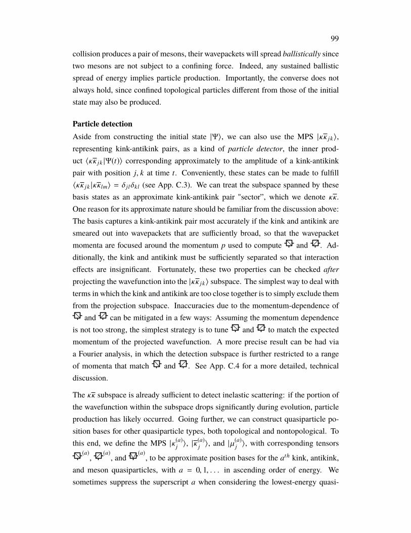
99

collision produces a pair of mesons, their wavepackets will spread ballistically sincetwo mesons are not subject to a confining force. Indeed, any sustained ballisticspread of energy implies particle production. Importantly, the converse does notalways hold, since confined topological particles different from those of the initialstate may also be produced.

Particle detectionAside from constructing the initial state |Ψ〉, we can also use the MPS |κκ j k〉,representing kink-antikink pairs, as a kind of particle detector, the inner prod-uct 〈κκ j k |Ψ(t)〉 corresponding approximately to the amplitude of a kink-antikinkpair with position j, k at time t. Conveniently, these states can be made to fulfill〈κκ j k |κκlm〉 = δ jlδkl (see App. C.3). We can treat the subspace spanned by thesebasis states as an approximate kink-antikink pair "sector”, which we denote κκ.One reason for its approximate nature should be familiar from the discussion above:The basis captures a kink-antikink pair most accurately if the kink and antikink aresmeared out into wavepackets that are sufficiently broad, so that the wavepacketmomenta are focused around the momentum p used to compute and . Ad-ditionally, the kink and antikink must be sufficiently separated so that interactioneffects are insignificant. Fortunately, these two properties can be checked afterprojecting the wavefunction into the |κκ j k〉 subspace. The simplest way to deal withterms in which the kink and antikink are too close together is to simply exclude themfrom the projection subspace. Inaccuracies due to the momentum-dependence of

and can be mitigated in a few ways: Assuming the momentum dependenceis not too strong, the simplest strategy is to tune and to match the expectedmomentum of the projected wavefunction. A more precise result can be had viaa Fourier analysis, in which the detection subspace is further restricted to a rangeof momenta that match and . See App. C.4 for a more detailed, technicaldiscussion.

The κκ subspace is already sufficient to detect inelastic scattering: if the portion ofthe wavefunction within the subspace drops significantly during evolution, particleproduction has likely occurred. Going further, we can construct quasiparticle po-sition bases for other quasiparticle types, both topological and nontopological. Tothis end, we define the MPS |κ(a)j 〉, |κ

(a)j 〉, and |µ

(a)j 〉, with corresponding tensors

(a),

(a), and

(a), to be approximate position bases for the ath kink, antikink,

and meson quasiparticles, with a = 0, 1, . . . in ascending order of energy. Wesometimes suppress the superscript a when considering the lowest-energy quasi-

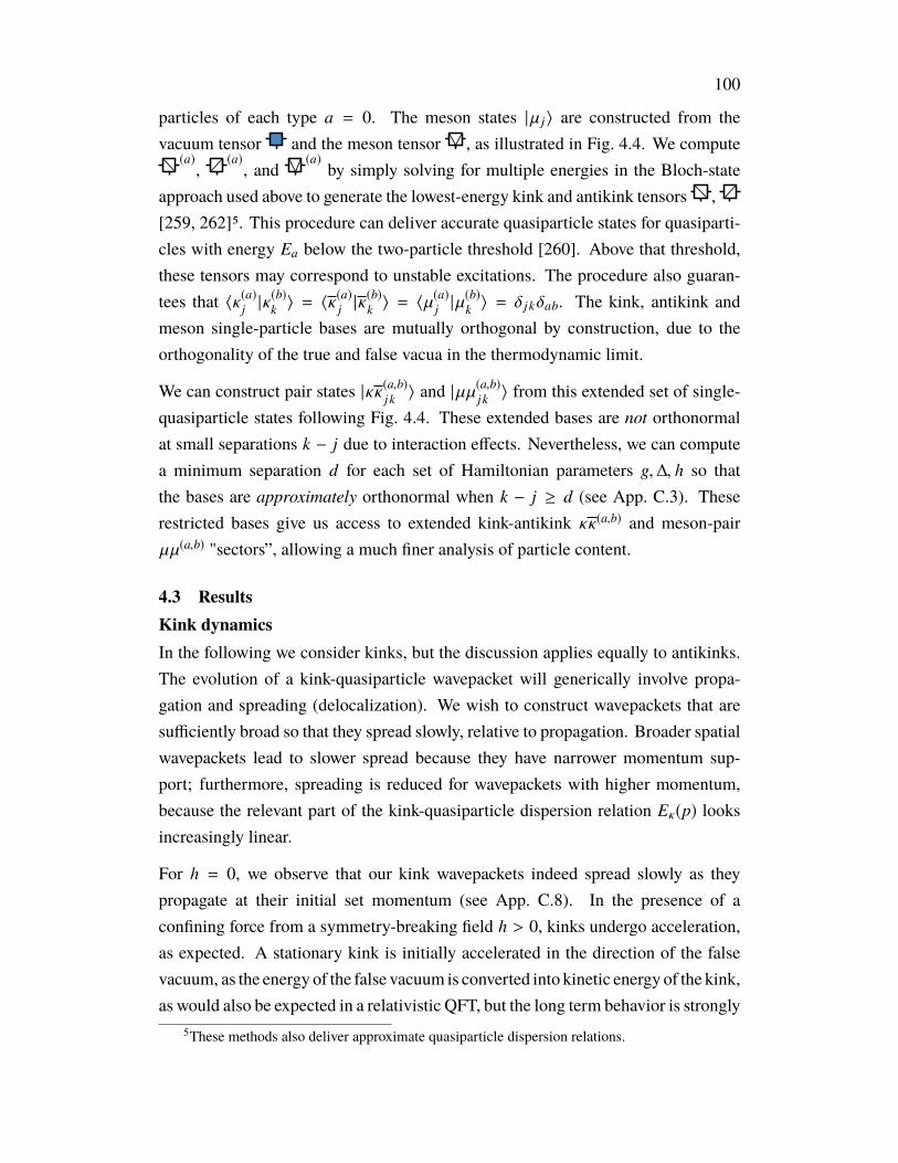
100

particles of each type a = 0. The meson states |µ j〉 are constructed from thevacuum tensor and the meson tensor , as illustrated in Fig. 4.4. We compute(a),

(a), and

(a)by simply solving for multiple energies in the Bloch-state

approach used above to generate the lowest-energy kink and antikink tensors ,[259, 262]5. This procedure can deliver accurate quasiparticle states for quasiparti-cles with energy Ea below the two-particle threshold [260]. Above that threshold,these tensors may correspond to unstable excitations. The procedure also guaran-tees that 〈κ(a)j |κ

(b)k 〉 = 〈κ

(a)j |κ

(b)k 〉 = 〈µ

(a)j |µ

(b)k 〉 = δ j kδab. The kink, antikink and

meson single-particle bases are mutually orthogonal by construction, due to theorthogonality of the true and false vacua in the thermodynamic limit.

We can construct pair states |κκ(a,b)j k 〉 and |µµ(a,b)j k 〉 from this extended set of single-

quasiparticle states following Fig. 4.4. These extended bases are not orthonormalat small separations k − j due to interaction effects. Nevertheless, we can computea minimum separation d for each set of Hamiltonian parameters g,∆, h so thatthe bases are approximately orthonormal when k − j ≥ d (see App. C.3). Theserestricted bases give us access to extended kink-antikink κκ(a,b) and meson-pairµµ(a,b) "sectors”, allowing a much finer analysis of particle content.

4.3 ResultsKink dynamicsIn the following we consider kinks, but the discussion applies equally to antikinks.The evolution of a kink-quasiparticle wavepacket will generically involve propa-gation and spreading (delocalization). We wish to construct wavepackets that aresufficiently broad so that they spread slowly, relative to propagation. Broader spatialwavepackets lead to slower spread because they have narrower momentum sup-port; furthermore, spreading is reduced for wavepackets with higher momentum,because the relevant part of the kink-quasiparticle dispersion relation Eκ(p) looksincreasingly linear.

For h = 0, we observe that our kink wavepackets indeed spread slowly as theypropagate at their initial set momentum (see App. C.8). In the presence of aconfining force from a symmetry-breaking field h > 0, kinks undergo acceleration,as expected. A stationary kink is initially accelerated in the direction of the falsevacuum, as the energy of the false vacuum is converted into kinetic energy of the kink,as would also be expected in a relativistic QFT, but the long term behavior is strongly

5These methods also deliver approximate quasiparticle dispersion relations.

101

influenced by the lattice (see App. C.7 for single-kink simulation data). The latticemomentum p is bounded −π < p ≤ π, and the momentum expectation value of thekink wavepacket precesses around the unit circle with Ûp = constant. To understandhow the position of the kink evolves as this happens, wemust consider thewavepacketgroup velocity v(p) := ∂Eκ(p)/∂p. With an emergent relativistic QFT governing theIR physics, the dispersion relation is approximately relativistic (Eκ(p) ∼

√p2 + m2

κ

for a kink of mass mκ) for small |p|, becoming almost linear as p increases. However,due to the bounded nature of p on the lattice, Eκ(p) must deviate from relativisticbehavior as |p| continues to increase. Indeed, assuming Eκ(p) is smooth, includingat the boundary value Eκ(π) = Eκ(−π), it is also bounded from above and below. Assuch, a wavepacket will typically reach a maximum group velocity for some p(vmax),after which it will begin to slow down. Assuming Eκ(p) = Eκ(−p) it will ultimatelyreverse and retrace its path back to its original position and momentum (with somewavepacket spread), performing Bloch oscillations.

Bubble dynamicsInstead of Bloch oscillations of individual kinks, we wish to study the emergentrelativistic dynamics of false-vacuum bubbles comprised of a kink wavepacket andan antikink wavepacket. In particular, we want to simulate kink-antikink collisionsat large kinetic energies (to increase particle-production amplitudes). Since the kinkand antikink accelerate toward each other under the confining force, we can increasethe kinetic energy at the time of collision by increasing the initial bubble size xR− xL

(and hence the amount of energy stored in the false vacuum). However, if we allowthe kink and antikink to evolve for too long prior to collision, their momenta willexceed |p(vmax)| and they will begin to undergo Bloch oscillations, deviating fromtheir relativistic behavior. We can ensure that this does not occur by limiting theinitial bubble size, with themaximum size depending on theHamiltonian parametersg, λ, h. In general, a smaller mass gap (since h , 0, this is the meson mass mµ),measured in lattice units, increases the maximum bubble size, measured in physicalunits (multiples of the lattice correlation length ξ). Moving closer to criticality thusallows us to reach higher collision energies relative to the mass gap while stayingbelow p(vmax).

We simulated bubble dynamics for the Ising model (λ = 0) as well as near to theTri-Critical Ising point of the extended model (λ > 0) for a range of parameters. Wefirst focus on the two points marked (i) and (ii) in Fig. 4.3.

102

200

400tim

e

(i) Ising (ii) near TCI

0 250 500 750position

200

400

time

0 250 500 750position

1.0

0.5

0.0

0.5

1.0

Z

6

4

2

log(

|e/E

|)

Figure 4.5: Spin expectation values and relative energy density e/E for (i) the Isingmodel (λ = 0, g = 0.8, h = 0.007) and (ii) the generalized Ising model nearer tothe Tricritical Ising CFT fixed point (TCI) (λ = 0.41, g = 0.98, h = 0.001). For (i),the initial wavepackets have σ = 25 and are 248.5 sites apart (E/mµ = 3.72). For(ii), σ = 40 with separation 287.4 (E/mµ = 2.62). The MPS bond dimensions areD = 10 and D = 18 for the vacua of (i) and (ii), respectively. During the simulationthe dimensions are restricted to D ≤ 128 and the integration step size is δt = 0.05.

The Ising modelIn the Ising case (λ = 0) with h = 0, known to be a theory of free kinks, oursimulations reproduce the expected trivial scattering: kinks given an initial nonzeromomentum collide without generating any additional entanglement. With explicitsymmetry-breaking (0 < h 1) we find nontrivial scattering, as evidenced byentanglement between the post-collision kink wavepackets. However, even whenthe energy is significantly above the meson pair-production threshold E > 2mµ

there is no obvious ballistic spread to indicate production of unconfined particles(see Fig. 4.5). Furthermore, the system is found to be within the bubble "sector”κκ(0,0) after the first collision to high numerical precision, as shown for g = 0.8 inFig. 4.6, consistent with purely elastic scattering of kinks. The probability 1 − Pκκof being in a different sector is estimated to be around O(10−5) both before andafter the first collision, with the difference closing as the maximum bond dimension

103

0 100 200 300 400 500time

10 6

10 5

10 4

10 3

10 2

10 1

100

P( n

ot in

su

bspa

ce )

(i) Ising: D 32(i) Ising: D 64(i) Ising: D 128(ii) near TCI: D 32(ii) near TCI: D 64(ii) near TCI: D 128

Figure 4.6: Portion of state (by probability) outside of the MPS bubble subspaceκκ(0,0) for simulations (i) and (ii) of Fig. 4.5. Here we fully account for momentumdependence of the basis states |κκ j,k〉 via a Fourier analysis and count only contri-butions with k − j ≥ 60 (see App. C.4). For Ising (i), the small probability afterthe first collision of t ≈ 90 indicates elastic scattering of kinks, in stark contrastwith the TCI case (ii), where the probability remains high after the first collisionat t ≈ 150. In (i), the growth of the post-collision probability with subsequentcollisions is consistent with increasingly inaccurate representation of accumulatingentanglement (due to the limit imposed on the MPS bond dimension D), as wellwith delocalization of the wavepackets, since contributions from kink-antikink pairswith small separation k − j are not counted.

increases. This probability is consistent with a numerical estimate of the accuracyof the kink-antikink quasiparticle basis states, as detailed in App. C.3. That Pκκ < 1during collisions, as well as later in the evolution as the wavepackets delocalize,is due to components of the state leaving the space of well-separated localizedquasiparticles as the kink and antikink interact. While we cannot entirely rule outinelastic scattering using this data, any inelastic process would have to be extremelyunlikely to be consistent with our results.

This observation is surprising given that the spin chain and its emergent field theoryare not integrable, but consistent with recent observations of nonthermalizing statesin the Ising model [236, 253, 254]. We further find that elastic scattering persistseven if we allow the kink velocity to exceed vmax, as it does in simulation (i) ofFigs. 4.5 and 4.6 (see App. C.7), so that the emergent relativistic field theory is

104

0.0 0.1 0.2 0.3 0.4 0.5 0.6momentum

0.2

0.4

0.6

0.8

1.0

1.2

ener

gy (r

elat

ive

to v

acuu

m)

(0)

(0)

(1)

(1)(0, 0) threshold

(0, 1) threshold(0, 1) threshold

(h = 0) (h = 0.001) (h = 0)

Figure 4.7: Dispersion relations (numerical, using MPS) of kinks κ and mesons µfor λ = 0.41, g = 0.98. For mesons, energies are shown with and without a weaklongitudinal field. Individual kinks do not have a finite energy for h > 0. Thresholdenergies for pair production are shown (computed assuming h = 0 for kinks andh = 0.001 for mesons), as is the energy (labelled Ψ) of the simulation shown inFig. 4.5 for parameter-set (ii).

no longer a good description of the physics. This is strong evidence that, in theIsing chain with a weak longitudinal field, bubbles are stable up to arbitrarily highenergies: When a bubble is large enough, its walls will not meet due to Blochoscillations, so no scattering can occur while it remains localized. When bubblesare small enough for the kinks to collide, our evidence suggests they always do soelastically.

Near the Tri-Critical Ising pointTurning on λ > 0, we choose the initial bubble size so that the energy, shown inFig. 4.7, is well above the pair-production threshold (but still low enough to keep thekink velocity vmax). Here we find clear evidence that unconfined particles are pro-duced. Most apparently, Fig. 4.5 (ii) clearly shows ballistic spread of wavepacketsemanating from the first collision event. To further resolve the scattering outcomes,we project onto meson-pair and kink-antikink-pair quasiparticle bases, finding fourdominant "sectors”, illustrated in Fig. 4.8, wherewe tune the quasiparticle basisMPSto match the momentum expectation value of the outgoing quasiparticle wavepack-ets (as estimated from the Fourier transform of the projected wavefunctions) and

105

1.0

0.5

0.0

0.5

1.0

Z

(0, 0) (P = 62%)

D 32D 64D 128

D 32D 64D 128

(P = 19%)

D 32D 64D 128

D 32D 64D 128

0 200 400 600 800position

1.0

0.5

0.0

0.5

1.0

Z

(0, 1) (P 7%)

D 32D 64D 128

D 32D 64D 128

0 200 400 600 800position

(1, 0) (P 7%)full (D 128)

Figure 4.8: Spin expectation values for simulation (ii) of Fig. 4.5 at time t = 270(bond dimension D ≤ 128) after projection into selected quasiparticle subspacesand normalization. The amount of wavefunction captured by each (approximatelyorthogonal) subspace is given as a probability P (see App. C.4). Included subspacesare µµ, a pair of mesons of lowest energy, and κκ(a,b), a bubble made of a kink oftype a and an antikink of type b (where 0 is the lowest-energy kink quasiparticle,and 1 is the next highest – see Fig. 4.7).

compute the spin expectation values of the projected wavefunction for each sector.We also compute the scattering outcome probabilities (the norms of the projectedwavefunctions)6. We find the most likely outgoing configurations to be: a bubblemade of type-0 kinks κκ(0,0) (elastic channel) with probability P = 62%, then atype-0 meson pair µµ(0,0) with P = 19%, and finally a bubble made either of atype-0 kink paired with a type-1 antikink (higher energy) κκ(0,1), or a type-1 kinkpaired with a type-0 antikink κκ(1,0), each with P ≈ 7% (reflection symmetry).These outcomes are all kinematically allowed, according to the energetic thresholdsshown in Fig. 4.7.

We note that the (rounded) projection probabilities in Fig. 4.8 only add to 95%.6For this we use amore sophisticated Fourier analysis that more fully accounts for themomentum

dependence of the quasiparticle basis MPS. see App. C.4.

106

This may indicate the presence of other sectors we have not accounted for, such asa µ(0) paired with a small κκ(0,0) bubble, or a κκ(0,0) bubble containing one or morequasiparticle-excitations of the false vacuum. Unfortunately, since these "sectors”each involve at least three quasiparticles, the corresponding position bases havemany more terms (O(N3) versus O(N2) for pairs), making them difficult to workwith7.

It is also possible that various sources of error have affected results: (i) when ex-citation tensors in a 2-quasiparticle MPS are close together, so that interactionsare relevant, the state may not accurately represent quasiparticles, (ii) the MPSrepresentations of the quasiparticle position states are variational approximationssubject to some error (which also affects the initial state of the simulation), and(iii) although we allow the MPS bond dimension to increase up to some maximumduring simulations (D ≤ 128 in this case), errors can still accumulate if that max-imum is insufficient to capture all entanglement, as well as due to errors in thenumerical integration steps. We did not explicitly characterize the effects of (ii),but expect them to be small, because the true and false vacuum MPS, upon whichthe excitations are built, are already accurate to ∼ 10−6 in norm. By varying theminimum quasiparticle separation used in the projection, as well as the maximumbond dimension of the simulation, we were able to characterize effects (i) and (iii),finding them to amount to changes in the outcome probabilities of 0.01, except inthe case of κκ(0,1) and κκ(1,0), in which one of the quasiparticles is heavier than theother, leading to a smaller separation between the kink and antikink. In this case,our analysis suggests the error here amounts to a change of around ±0.01 in theoutcome probability, possibly more (see App. C.4). This outcome might be betterresolved at higher energies, at which the kink-antikink separations would increase.

In case of the µµ outcome, we cross-check the computed outcome probability bycomparing it with the excess energy (relative to the vacuum) Epkts of the regionscontaining the ballistic wavepackets, visible in Fig. 4.5 (ii). If these wavepacketsbelong to a two-meson "branch” of the wavefunction, that branch (the portion ofthe wavefunction in the µµ subspace) must contribute EP to the energy, where E

is the total energy and P is the probability of the µµ scattering outcome. We cantherefore estimate P as Epkts/E . This gives us a P within the range 19% to 20%at t = 480 (after separation), depending on the precise extent of the region we sumover (e.g. from site 0 to site 250 for the left packet), compatible with the projected

7Not only computationally, but also because basis orthogonality is harder to achieve.

107

12345

max

. cut

ent

ropy

(i) Ising

D 32D 64D 128 1

2345

(ii) near TCI

D 32D 64D 128

200 400 600 800time

200

400

600cut p

ositi

on

D 128200 400

time

250

500

750 D 128 12345

cut e

ntro

py

Figure 4.9: Entanglement entropy (base 2) for cuts (left-right bipartitions) of the spinchain as a function of time for the simulations (i) and (ii) of Fig. 4.5. Convergencewith the bond dimension D slows as time goes on. For example, in (i) the max. cutentropy at D ≤ 128 is very likely not converged after t ≈ 400.

µµ wavefunction.

Entropy and computational costAs evidenced by Fig. 4.6, the bond dimension of the MPS representing the evolvingstate must continue to grow as time goes on, in order to maintain accuracy. Thecut entropy at location j is a proxy for the required bond dimension D j . Fig. 4.9shows the evolution of the maximum cut entropy for the simulations of Fig. 4.5. Atearly times, we observe that the maximum cut entropy jumps dramatically duringscattering events, whether elastic or inelastic, remaining almost constant in between.This is consistent with a model of interacting quasiparticle wavepackets: Separatedwavepackets undergo stable propagation until they collide, at which point inter-actions generate entanglement corresponding to the different possible scatteringoutcomes. At late times, we observe a temporal broadening of the jumps, con-sistent with spatial broadening of the wavepackets involved. Fig. 4.9 also showsthat, although there is cut entropy associated with the wavepackets themselves, thisis quickly surpassed by the cut entropy in the center of the chain, associated withentanglement between the left and right outgoing packets. It is this entanglementbetween outgoing quasiparticles that is responsible for the post-collision plateausvisible in the maximum cut entropy.

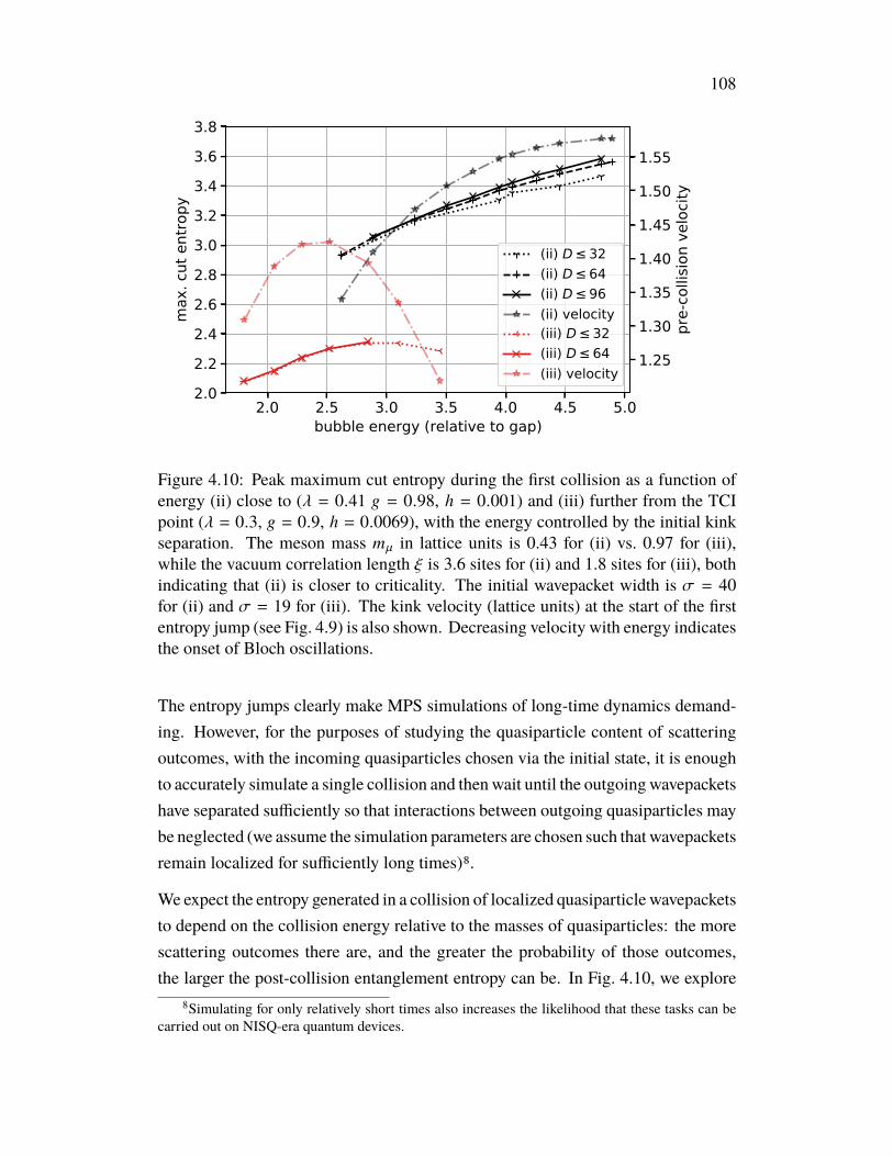
108

2.0 2.5 3.0 3.5 4.0 4.5 5.0bubble energy (relative to gap)

2.02.22.42.62.83.03.23.43.63.8

max

. cut

ent

ropy

1.25

1.30

1.35

1.40

1.45

1.50

1.55

pre-

collis

ion

velo

city

(ii) D 32(ii) D 64(ii) D 96(ii) velocity(iii) D 32(iii) D 64(iii) velocity

Figure 4.10: Peak maximum cut entropy during the first collision as a function ofenergy (ii) close to (λ = 0.41 g = 0.98, h = 0.001) and (iii) further from the TCIpoint (λ = 0.3, g = 0.9, h = 0.0069), with the energy controlled by the initial kinkseparation. The meson mass mµ in lattice units is 0.43 for (ii) vs. 0.97 for (iii),while the vacuum correlation length ξ is 3.6 sites for (ii) and 1.8 sites for (iii), bothindicating that (ii) is closer to criticality. The initial wavepacket width is σ = 40for (ii) and σ = 19 for (iii). The kink velocity (lattice units) at the start of the firstentropy jump (see Fig. 4.9) is also shown. Decreasing velocity with energy indicatesthe onset of Bloch oscillations.

The entropy jumps clearly make MPS simulations of long-time dynamics demand-ing. However, for the purposes of studying the quasiparticle content of scatteringoutcomes, with the incoming quasiparticles chosen via the initial state, it is enoughto accurately simulate a single collision and thenwait until the outgoing wavepacketshave separated sufficiently so that interactions between outgoing quasiparticles maybe neglected (we assume the simulation parameters are chosen such that wavepacketsremain localized for sufficiently long times)8.

We expect the entropy generated in a collision of localized quasiparticle wavepacketsto depend on the collision energy relative to the masses of quasiparticles: the morescattering outcomes there are, and the greater the probability of those outcomes,the larger the post-collision entanglement entropy can be. In Fig. 4.10, we explore

8Simulating for only relatively short times also increases the likelihood that these tasks can becarried out on NISQ-era quantum devices.

109

the maximum cut entropy as a function of energy, controlled via the initial kinkseparation, for two sets of Hamiltonian parameters, one (ii) closer and one (iii)further from criticality. We find that the entropy indeed grows with energy, smoothlyincreasing even as thresholds are crossed, e.g. the 2mµ(1) , 3mµ(0) , and 4mµ(0) thresholdsin case of (ii) (see also Fig. 4.7).

The entropy continues to increase at least until the energy is sufficient for the kinksto approach the maximum possible kink velocity prior to collision, at which pointwe expect deviations from the emergent relativistic dynamics to become apparentas Bloch oscillations emerge. In the case of (iii), Fig. 4.10 shows that the post-collision entropy eventually decreases as lattice effects kick in, coincident withdeceleration of the kinks prior to collision. Note that we are able to reach muchhigher relative energies with parameters (ii) before encountering obvious latticeeffects. This illustrates the general principle that more of the emergent relativisticQFT is revealed as one approaches criticality: the relative energies accessible byquasiparticles, while avoiding Bloch oscillations (momenta < p(vmax)), grows asthe lattice meson mass drops.

We also observe that much more entropy is generated in the first collision forparameters (ii) than for parameters (iii), even when the relative energy is similar9.A significant part of this difference likely comes from a much higher probability ofmeson pair production, as well as the availability of the κκ(0,1) outcomes, in case (ii):the probability of particle production is < 10% in case (iii) at energy E/mµ ≈ 2.52,in contrast with ∼ 38% at energy E/mµ ≈ 2.62 in case (ii), according to κκ(0,0) basisoverlaps. This is possible, since these two parameter sets were not chosen to be partof an RG trajectory, so that their emergent QFTs need not be the same.

4.4 DiscussionBuilding on recent innovations in the classical simulation of quasiparticle dynamicsusing Matrix Product States [239], we proposed a framework for simulating andcharacterizing the full (nonperturbative) quantumdynamics of false-vacuumbubblesin relativistic QFTs that govern the IR physics of one-dimensional lattice systems.While we chose to simulate a quantum spin chain, the methods we use are generaland could also be applied directly to, for instance, a spatially-discretized QFT suchas the Schwinger model or λφ4 theory [2, 28, 207–212, 241]. We also demonstratedthat the MPS quasiparticle ansatz, with which we initialized our simulations, can

9The difference in post-collision entropy is not attributable to different vacuum entropies, sincethese are < 0.1 in both cases.

110

be used to detect quasiparticles that are produced as time evolves. This allowedus to verify quasiparticle pair-production in the modified Ising model we studied,including production of different species of confined kink that were not obvious fromexamining energy density and spin expectation values alone. We used the same kindof analysis to confirm a lack of particle-production in the unmodified Ising model(with transverse field and small longitudinal field), supporting other recent studiesthat suggest particle production is very strongly suppressed [236, 253, 254].

We were able to significantly improve the efficiency and interpretability of oursimulations by carefully choosing our initial states in two different ways: Firstly,constructing spatially broad wavepackets allowed us to access the dynamics of theemergent IR QFT without the spoiling effects of UV, high-momentum componentsthat are strongly influenced by the lattice. Broad wavepackets also lead to local-ization of quasiparticles over long times, making it easier to characterize scatteringoutcomes, and improve the numerical conditioning of the dynamical simulation(see App. C.6). Secondly, by precisely tuning the quasiparticle content of the initialwavepackets [239], we were able to study individual scattering events in isolation,while further reducing the computational demands of the simulation by loweringentanglement.

Entanglement growth is the most significant barrier to dynamical simulations withMPS, as the computational cost of each time step scales exponentially with the cutentropy. By choosing broad quasiparticle wavepackets, we reduce entanglementgrowth at the expense of growing the number of lattice sites involved in the simula-tion. This is a good tradeoff for MPS simulations, as the computational cost scalesonly linearly in the number of lattice sites. Even with this tradeoff, we found thatthe large jumps in cut entanglement with each collision (of confined quasiparticlesin the system) preclude simulating more than a handful of successive collisions.Furthermore, we found clear evidence of entanglement growth with the collisionenergy, although the onset of Bloch oscillations prevented us from drawing strongconclusions about how this growth continues in the emergent IR QFT. Nevertheless,in the absence of lattice effects that obscure the IR QFT, it seems reasonable to ex-pect the entropy to continue to grow with energy, which would eventually precludeaccurate simulation using MPS.

A natural next stepwould be to identify RG trajectories in the Hamiltonian parameterspace so that results can be extrapolated to the continuum. This is equivalent tofinding paths toward criticality of the lattice model, along which the low-energy

111

spectrum remains consistent with a particular emergent (IR) QFT. Moving closer tothe continuumwould also allow us to reach higher (relative) collision energies whileavoiding lattice effects, such as Bloch oscillations. In turn, this would permit a morethorough exploration of the energy-dependence of the entanglement generated incollisions.

As we approach criticality, the bond dimension of the MPS vacua must grow tomaintain accuracy, as must the size of the simulation window, since the wavepacketwidth in lattice units would have to increase with the lattice correlation length inorder to maintain localization. Getting closer to criticality seems feasible: Thesimulations featured in the main text, with maximumMPS bond dimension 128 andtime-step size 0.05, took between one and two weeks to complete on 8 cores eachand this time could likely be reduced significantly with further work to optimize thecode10 and the use of a numerical integrator with an adaptive time-step size.

Increasing the number of spatial dimensions presents a significantly greater chal-lenge for classical algorithms: while the computational cost of MPS simulationsscales with the bond dimension D as O(D3), the scaling for tensor-networks capableof handling large (2+1)-dimensional systems, such as PEPS [267], is much worse(albeit still polynomial)11. As an intermediate step, one could consider systems witha small, compactified second dimension of space, which are often within reach ofMPS methods. By performing a Fourier transform of the Hamiltonian in the com-pactified direction only [269], one could study scattering of quasiparticles that arespatially localized in one direction, while being momentum eigenstates of the other.Compared to the purely (1+1)-dimensional case, the additional "Kaluza-Klein” ex-citations associated with the Fourier modes of the compactified dimension wouldalready open up a much greater range of scattering outcomes.

Compared to the simulations we performed, increasing the variety of scatteringoutcomes, whether by raising the relative energy in a given model, choosing alattice model with a richer set of low-energy excitations (e.g. near a phase transitiondescribed by a CFT with larger central charge), or adding spatial dimensions, seemsnecessary in order to find problems that exhaust tensor-network methods due tothe additional entanglement generated. Such problems appear more amenable to

10GPU acceleration may also be useful [266].11Some methodological changes would also be needed: false-vacuum bubbles in > 1 spatial di-

mensions, having extensive boundaries, no longer look like mesons. As such, localized quasiparticletechniques (such as those developed for PEPS [268]) are not directly applicable. Instead, suitableinitial states could likely be prepared via energy minimization in the presence of a nonuniformsymmetry-breaking field.

112

simulation on quantum hardware, which is not a priori limited in the amount ofentanglement it can deal with. However, raising the energy may be problematic fornear-term quantum devices, which are limited both in their size and coherence times,since avoiding lattice effects (such as Bloch oscillations) at higher relative energiesrequires moving closer to criticality while increasing system sizes and evolutiontimes. Instead, increasing the richness of low-energy excitations by changing themodel or adding (compactified) dimensions, while avoiding coming too close tocriticality, may be a more promising route toward quantum advantage using near-term devices.

Acknowledgments

We thank Alex Buser, Marcela Carena, Cliff Cheung, Natalie Klco, Ying-Ying Li,Spiros Michalakis, Nicola Pancotti, Burak Şahinoğlu, Martin Savage, and EugeneTang for useful discussions and comments.

This material is based upon work supported in part by the U.S. Department ofEnergy Office of Science, Office of Advanced Scientific Computing Research, (DE-NA0003525, DE-SC0020290), and Office of High Energy Physics (DE-ACO2-07CH11359, DE-SC0018407).

AM, JL, and JP also acknowledge funding provided by the Institute for Quantum In-formation andMatter, an NSF Physics Frontiers Center (NSF Grant PHY-1733907),the Simons Foundation It from Qubit Collaboration, and the Air Force Office ofScientific Research (FA9550-19-1-0360). GV is a CIFAR fellow in the QuantumInformation Science Program. Sandbox is a team within the Alphabet family ofcompanies, which includes Google, Verily, Waymo, X, and others. Research atPerimeter Institute is supported in part by the Government of Canada through theDepartment of Innovation, Science and Economic Development Canada and by theProvince of Ontario through the Ministry of Colleges and Universities. Some ofthe computations presented here were conducted on the Caltech High PerformanceCluster, partially supported by a grant from theGordon andBettyMoore Foundation.

113

BIBLIOGRAPHY

[1] S. Durr et al., “Ab-Initio Determination of Light Hadron Masses,” Science322 (2008) 1224–1227, arXiv:0906.3599 [hep-lat].

[2] J. Liu, J. Preskill, and B. Şahinoğlu, “Simulating kink scattering in aquantum computer,” to appear.https://drive.google.com/file/d/1wOrPmO7lfutZlLEj-12JiMUAVg4nOdQr/view.

[3] A. Milsted, J. Liu, J. Preskill, and G. Vidal, “Collisions of false-vacuumbubble walls in a quantum spin chain,” arXiv:2012.07243 [quant-ph].

[4] S. M. Chester, W. Landry, J. Liu, D. Poland, D. Simmons-Duffin, N. Su, andA. Vichi, “Carving out OPE space and precise O(2) model criticalexponents,” JHEP 06 (2020) 142, arXiv:1912.03324 [hep-th].

[5] J. Liu, D. Meltzer, D. Poland, and D. Simmons-Duffin, “The Lorentzianinversion formula and the spectrum of the 3d O(2) CFT,” JHEP 09 (2020)115, arXiv:2007.07914 [hep-th].

[6] E. Palti, “The Swampland: Introduction and Review,” Fortsch. Phys. 67no. 6, (2019) 1900037, arXiv:1903.06239 [hep-th].

[7] M. Hasenbusch, “Monte Carlo study of a generalized icosahedral model onthe simple cubic lattice,” Phys. Rev. B 102 no. 2, (2020) 024406,arXiv:2005.04448 [cond-mat.stat-mech].

[8] M. Hasenbusch and E. Vicari, “Anisotropic perturbations inthree-dimensional o(n)-symmetric vector models,” Physical Review B 84no. 12, (Sep, 2011) 125136.http://dx.doi.org/10.1103/PhysRevB.84.125136.

[9] E. O’Brien and P. Fendley, “Lattice supersymmetry and order-disordercoexistence in the tricritical Ising model,” Phys. Rev. Lett. 120 no. 20,(2018) 206403, arXiv:1712.06662 [cond-mat.stat-mech].

[10] N. Sannomiya and H. Katsura, “Supersymmetry Breaking andNambu-Goldstone Fermions in Interacting Majorana Chains,” Phys. Rev. D99 no. 4, (2019) 045002, arXiv:1712.01148 [cond-mat.str-el].

[11] P. Fonseca and A. Zamolodchikov, “Ising spectroscopy. I. Mesons at T <T(c),” 12, 2006.

[12] G. Mussardo and G. Takacs, “Effective potentials and kink spectra innon-integrable perturbed conformal field theories,” J. Phys. A 42 (2009)304022, arXiv:0901.3537 [hep-th].

114

[13] P. Calabrese, A. Pelissetto, and E. Vicari, “Critical structure factors ofbilinear fields in o(n) vector models,” Physical Review E 65 no. 4, (Apr,2002) 046115. http://dx.doi.org/10.1103/PhysRevE.65.046115.

[14] E. Schrödinger, “Nature and the greeks, science and humanism,”.

[15] “See, https://www.forbes.com/sites/niallmccarthy/2016/01/06/americas-best-phd-majors-by-salary-infographic/?sh=1596ba603ed5,”.

[16] “See, https://www.ftc.gov/news-events/press-releases/2019/07/ftc-imposes-5-billion-penalty-sweeping-new-privacy-restrictions,”.

[17] N. Y. Halpern, “Quantum steampunk: Quantum information,thermodynamics, their intersection, and applications thereof acrossphysics,” PhD. Thesis, Caltech, 2018, arxiv:1807.09786 (2018) .

[18] Z. Ahmed et al., “Quantum Sensing for High Energy Physics,” in Firstworkshop on Quantum Sensing for High Energy Physics. 3, 2018.arXiv:1803.11306 [hep-ex].

[19] D. Simmons-Duffin, “The Conformal Bootstrap,” in Theoretical AdvancedStudy Institute in Elementary Particle Physics: New Frontiers in Fields andStrings, pp. 1–74. 2017. arXiv:1602.07982 [hep-th].

[20] L. F. Alday, J. Maldacena, A. Sever, and P. Vieira, “Y-system for ScatteringAmplitudes,” J. Phys. A 43 (2010) 485401, arXiv:1002.2459 [hep-th].

[21] J. M. Maldacena, “The Large N limit of superconformal field theories andsupergravity,” Int. J. Theor. Phys. 38 (1999) 1113–1133,arXiv:hep-th/9711200.

[22] R. P. Feynman, “Simulating physics with computers,” Int. J. Theor. Phys. 21(1982) 467–488.

[23] J. Preskill, “Simulating quantum field theory with a quantum computer,”PoS LATTICE2018 (2018) 024, arXiv:1811.10085 [hep-lat].

[24] J. Preskill, “Quantum computing in the nisq era and beyond,” Quantum 2(2018) 79.

[25] F. Arute, K. Arya, R. Babbush, D. Bacon, J. C. Bardin, R. Barends,R. Biswas, S. Boixo, F. G. Brandao, D. A. Buell, et al., “Quantumsupremacy using a programmable superconducting processor,” Nature 574no. 7779, (2019) 505–510.

[26] G. Ortiz, J. Gubernatis, E. Knill, and R. Laflamme, “Quantum algorithmsfor fermionic simulations,” Phys. Rev. A 64 (2001) 022319,arXiv:cond-mat/0012334. [Erratum: Phys.Rev.A 65, 029902 (2002)].

115

[27] S. P. Jordan, K. S. Lee, and J. Preskill, “Quantum Algorithms for QuantumField Theories,” Science 336 (2012) 1130–1133, arXiv:1111.3633[quant-ph].

[28] S. P. Jordan, K. S. Lee, and J. Preskill, “Quantum Computation of Scatteringin Scalar Quantum Field Theories,” Quant. Inf. Comput. 14 (2014)1014–1080, arXiv:1112.4833 [hep-th].

[29] S. P. Jordan, K. S. M. Lee, and J. Preskill, “Quantum Algorithms forFermionic Quantum Field Theories,” arXiv:1404.7115 [hep-th].

[30] S. P. Jordan, H. Krovi, K. S. M. Lee, and J. Preskill, “BQP-completeness ofScattering in Scalar Quantum Field Theory,” arXiv:1703.00454[quant-ph].

[31] S. R. Coleman, “Classical Lumps and their Quantum Descendents,”Subnucl. Ser. 13 (1977) 297.

[32] T. Lee and Y. Pang, “Nontopological solitons,” Phys. Rept. 221 (1992)251–350.

[33] G. F. Chew, “S-Matrix Theory of Strong Interactions without ElementaryParticles,” Rev. Mod. Phys. 34 no. 3, (1962) 394–401.

[34] A. Polyakov, “Nonhamiltonian approach to conformal quantum fieldtheory,” Zh. Eksp. Teor. Fiz. 66 (1974) 23–42.

[35] D. Simmons-Duffin, “A Semidefinite Program Solver for the ConformalBootstrap,” JHEP 06 (2015) 174, arXiv:1502.02033 [hep-th].

[36] S. El-Showk, M. F. Paulos, D. Poland, S. Rychkov, D. Simmons-Duffin, andA. Vichi, “Solving the 3D Ising Model with the Conformal Bootstrap,”Phys. Rev. D 86 (2012) 025022, arXiv:1203.6064 [hep-th].

[37] S. Caron-Huot, “Analyticity in Spin in Conformal Theories,” JHEP 09(2017) 078, arXiv:1703.00278 [hep-th].

[38] S. M. Chester, W. Landry, J. Liu, D. Poland, D. Simmons-Duffin, N. Su, andA. Vichi, “Bootstrapping Heisenberg Magnets and their Cubic Instability,”arXiv:2011.14647 [hep-th].

[39] W. Landry and D. Simmons-Duffin, “Scaling the semidefinite programsolver SDPB,” arXiv:1909.09745 [hep-th].

[40] N. Bao and J. Liu, “Quantum algorithms for conformal bootstrap,” Nucl.Phys. B 946 (2019) 114702, arXiv:1811.05675 [hep-th].

[41] CMS Collaboration, A. M. Sirunyan et al., “Identification of heavy,energetic, hadronically decaying particles using machine-learningtechniques,” JINST 15 no. 06, (2020) P06005, arXiv:2004.08262[hep-ex].

116

[42] T. Roxlo and M. Reece, “Opening the black box of neural nets: case studiesin stop/top discrimination,” arXiv:1804.09278 [hep-ph].

[43] R. Bousso and J. Polchinski, “Quantization of four form fluxes anddynamical neutralization of the cosmological constant,” JHEP 06 (2000)006, arXiv:hep-th/0004134.

[44] L. Susskind, “The Anthropic landscape of string theory,”arXiv:hep-th/0302219.

[45] S. Ashok and M. R. Douglas, “Counting flux vacua,” JHEP 01 (2004) 060,arXiv:hep-th/0307049.

[46] C. Cheung, J. Liu, and G. N. Remmen, “Proof of the Weak GravityConjecture from Black Hole Entropy,” JHEP 10 (2018) 004,arXiv:1801.08546 [hep-th].

[47] F. Denef and M. R. Douglas, “Computational complexity of the landscape.I.,” Annals Phys. 322 (2007) 1096–1142, arXiv:hep-th/0602072.

[48] M. R. Douglas, “Spaces of Quantum Field Theories,” J. Phys. Conf. Ser.462 no. 1, (2013) 012011, arXiv:1005.2779 [hep-th].

[49] F. Denef, M. R. Douglas, B. Greene, and C. Zukowski, “Computationalcomplexity of the landscape II—Cosmological considerations,” AnnalsPhys. 392 (2018) 93–127, arXiv:1706.06430 [hep-th].

[50] J. Liu, “Artificial Neural Network in Cosmic Landscape,” JHEP 12 (2017)149, arXiv:1707.02800 [hep-th].

[51] Y.-H. He, “Deep-Learning the Landscape,” arXiv:1706.02714[hep-th].

[52] F. Ruehle, “Data science applications to string theory,” Phys. Rept. 839(2020) 1–117.

[53] J. Halverson and C. Long, “Statistical Predictions in String Theory andDeep Generative Models,” Fortsch. Phys. 68 no. 5, (2020) 2000005,arXiv:2001.00555 [hep-th].

[54] S. Hawking, “Particle Creation by Black Holes,” Commun. Math. Phys. 43(1975) 199–220. [Erratum: Commun.Math.Phys. 46, 206 (1976)].

[55] S. Hawking, “Black hole explosions,” Nature 248 (1974) 30–31.

[56] S. Ryu and T. Takayanagi, “Holographic derivation of entanglement entropyfrom AdS/CFT,” Phys. Rev. Lett. 96 (2006) 181602,arXiv:hep-th/0603001.

117

[57] A. Almheiri, X. Dong, and D. Harlow, “Bulk Locality and Quantum ErrorCorrection in AdS/CFT,” JHEP 04 (2015) 163, arXiv:1411.7041[hep-th].

[58] P. Hayden and J. Preskill, “Black holes as mirrors: Quantum information inrandom subsystems,” JHEP 09 (2007) 120, arXiv:0708.4025 [hep-th].

[59] A. R. Brown, D. A. Roberts, L. Susskind, B. Swingle, and Y. Zhao,“Holographic Complexity Equals Bulk Action?,” Phys. Rev. Lett. 116no. 19, (2016) 191301, arXiv:1509.07876 [hep-th].

[60] “It from qubit, https://www.simonsfoundation.org/mathematics-physical-sciences/it-from-qubit/.,”.

[61] L. McGough, M. Mezei, and H. Verlinde, “Moving the CFT into the bulkwith TT ,” JHEP 04 (2018) 010, arXiv:1611.03470 [hep-th].

[62] P. Kraus, J. Liu, and D. Marolf, “Cutoff AdS3 versus the TT deformation,”JHEP 07 (2018) 027, arXiv:1801.02714 [hep-th].

[63] X. Dong, E. Silverstein, and G. Torroba, “De Sitter Holography andEntanglement Entropy,” JHEP 07 (2018) 050, arXiv:1804.08623[hep-th].

[64] V. Gorbenko, E. Silverstein, and G. Torroba, “dS/dS and TT ,” JHEP 03(2019) 085, arXiv:1811.07965 [hep-th].

[65] A. Lewkowycz, J. Liu, E. Silverstein, and G. Torroba, “TT and EE, withimplications for (A)dS subregion encodings,” JHEP 04 (2020) 152,arXiv:1909.13808 [hep-th].

[66] “The non-perturbative bootstrap,https://bootstrapcollaboration.com.,”.

[67] L. Susskind, “Horizons Protect Church-Turing,” arXiv:2003.01807[hep-th].

[68] M. Hogarth, Predictability, computability, and spacetime. PhD thesis,University of Cambridge, 1996.

[69] R. Geroch and J. B. Hartle, “Computability and physical theories,”Foundations of Physics 16 no. 6, (1986) 533–550.

[70] A. Bouland, B. Fefferman, and U. Vazirani, “Computationalpseudorandomness, the wormhole growth paradox, and constraints on theAdS/CFT duality,” arXiv:1910.14646 [quant-ph].

[71] I. Kim, E. Tang, and J. Preskill, “The ghost in the radiation: Robustencodings of the black hole interior,” JHEP 20 (2020) 031,arXiv:2003.05451 [hep-th].

118

[72] B. Yoshida, “Remarks on Black Hole Complexity Puzzle,”arXiv:2005.12491 [hep-th].

[73] E. Witten, “String theory dynamics in various dimensions,” Nucl. Phys. B443 (1995) 85–126, arXiv:hep-th/9503124.

[74] P.-S. Hsin and N. Seiberg, “Level/rank Duality and Chern-Simons-MatterTheories,” JHEP 09 (2016) 095, arXiv:1607.07457 [hep-th].

[75] E. H. Lieb and M. B. Ruskai, “A Fundamental Property ofQuantum-Mechanical Entropy,” Phys. Rev. Lett. 30 (1973) 434–436.

[76] E. Lieb and M. Ruskai, “Proof of the strong subadditivity ofquantum-mechanical entropy,” J. Math. Phys. 14 (1973) 1938–1941.

[77] M. Headrick and T. Takayanagi, “A Holographic proof of the strongsubadditivity of entanglement entropy,” Phys. Rev. D 76 (2007) 106013,arXiv:0704.3719 [hep-th].

[78] T. C. Bohdanowicz and F. G. Brandao, “Universal Hamiltonians forExponentially Long Simulation,” arXiv:1710.02625 [quant-ph].

[79] F. G. Brandao, W. Chemissany, N. Hunter-Jones, R. Kueng, and J. Preskill,“Models of quantum complexity growth,” arXiv:1912.04297 [hep-th].

[80] L. Susskind, “Computational Complexity and Black Hole Horizons,”Fortsch. Phys. 64 (2016) 24–43, arXiv:1403.5695 [hep-th].[Addendum: Fortsch.Phys. 64, 44–48 (2016)].

[81] P. Hayden and G. Penington, “Black hole microstates vs. the additivityconjectures,” arXiv:2012.07861 [hep-th].

[82] P. Mehta and D. J. Schwab, “An exact mapping between the variationalrenormalization group and deep learning,” arXiv preprint arXiv:1410.3831(2014) .

[83] E. Dyer and G. Gur-Ari, “Asymptotics of Wide Networks from FeynmanDiagrams,” arXiv:1909.11304 [cs.LG].

[84] A. R. Brown, H. Gharibyan, S. Leichenauer, H. W. Lin, S. Nezami,G. Salton, L. Susskind, B. Swingle, and M. Walter, “Quantum Gravity in theLab: Teleportation by Size and Traversable Wormholes,”arXiv:1911.06314 [quant-ph].

[85] D. M. Hofman and J. Maldacena, “Conformal collider physics: Energy andcharge correlations,” JHEP 05 (2008) 012, arXiv:0803.1467 [hep-th].

[86] S. W. Hawking, M. J. Perry, and A. Strominger, “Soft Hair on Black Holes,”Phys. Rev. Lett. 116 no. 23, (2016) 231301, arXiv:1601.00921[hep-th].

119

[87] L. J. Dixon, M.-X. Luo, V. Shtabovenko, T.-Z. Yang, and H. X. Zhu,“Analytical Computation of Energy-Energy Correlation at Next-to-LeadingOrder in QCD,” Phys. Rev. Lett. 120 no. 10, (2018) 102001,arXiv:1801.03219 [hep-ph].

[88] M. Kologlu, P. Kravchuk, D. Simmons-Duffin, and A. Zhiboedov, “Thelight-ray OPE and conformal colliders,” arXiv:1905.01311 [hep-th].

[89] “https://news.fnal.gov/2018/09/department-of-energy-awards-fermilab-more-than-10-million-for-quantum-science/,”.

[90] “http://www.xact.es,”.

[91] J. Polchinski, “Memories of a Theoretical Physicist,” arXiv:1708.09093[physics.hist-ph].

[92] “Private communications with Ning Su,”.

[93] “The man who knew infinity, https://en.wikipedia.org/wiki/The_Man_Who_Knew_Infinity_(film),”.

[94] G. Raayoni, S. Gottlieb, G. Pisha, Y. Harris, Y. Manor, U. Mendlovic,D. Haviv, Y. Hadad, and I. Kaminer, “The ramanujan machine:automatically generated conjectures on fundamental constants,” arXivpreprint arXiv:1907.00205 (2019) .

[95] “The ramanujan machine. http://www.ramanujanmachine.com/.,”.

[96] “Number theorist fears all published math is wrong.https://www.vice.com/en_us/article/8xwm54/number-theorist-fears-all-published-math-is-wrong-actually.,”.

[97] P. Huang, A. J. Long, and L.-T. Wang, “Probing the Electroweak PhaseTransition with Higgs Factories and Gravitational Waves,” Phys. Rev. D 94no. 7, (2016) 075008, arXiv:1608.06619 [hep-ph].

[98] S. Deser and P. van Nieuwenhuizen, “One Loop Divergences of QuantizedEinstein-Maxwell Fields,” Phys. Rev. D10 (1974) 401.

[99] R. M. Wald, “Black hole entropy is the Noether charge,” Phys. Rev. D48(1993) R3427, arXiv:gr-qc/9307038 [gr-qc].

[100] X. Dong, “Holographic Entanglement Entropy for General HigherDerivative Gravity,” JHEP 01 (2014) 044, arXiv:1310.5713 [hep-th].

[101] J. D. Bekenstein, “Black holes and entropy,” Phys. Rev. D7 (1973) 2333.

[102] S. W. Hawking, “Black Holes and Thermodynamics,” Phys. Rev. D13(1976) 191.

120

[103] P. C. W. Davies, “Thermodynamics of Black Holes,” Proc. Roy. Soc. Lond.A353 (1977) 499.

[104] N. Arkani-Hamed, L. Motl, A. Nicolis, and C. Vafa, “The string landscape,black holes and gravity as the weakest force,” JHEP 06 (2007) 060,arXiv:hep-th/0601001 [hep-th].

[105] C. Cheung and G. N. Remmen, “Naturalness and the Weak GravityConjecture,” Phys. Rev. Lett. 113 (2014) 051601, arXiv:1402.2287[hep-ph].

[106] C. Vafa, “The String Landscape and the Swampland,”arXiv:hep-th/0509212 [hep-th].

[107] H. Ooguri and C. Vafa, “On the Geometry of the String Landscape and theSwampland,” Nucl. Phys. B766 (2007) 21, arXiv:hep-th/0605264[hep-th].

[108] A. Adams, N. Arkani-Hamed, S. Dubovsky, A. Nicolis, and R. Rattazzi,“Causality, analyticity and an IR obstruction to UV completion,” JHEP 10(2006) 014, arXiv:hep-th/0602178 [hep-th].

[109] C. Cheung and G. N. Remmen, “Infrared Consistency and the Weak GravityConjecture,” JHEP 12 (2014) 087, arXiv:1407.7865 [hep-th].

[110] B. Bellazzini, C. Cheung, and G. N. Remmen, “Quantum GravityConstraints from Unitarity and Analyticity,” Phys. Rev. D93 (2016) 064076,arXiv:1509.00851 [hep-th].

[111] C. Cheung and G. N. Remmen, “Positive Signs in Massive Gravity,” JHEP04 (2016) 002, arXiv:1601.04068 [hep-th].

[112] C. Cheung and G. N. Remmen, “Positivity of Curvature-SquaredCorrections in Gravity,” Phys. Rev. Lett. 118 (2017) 051601,arXiv:1608.02942 [hep-th].

[113] G. W. Gibbons and S. W. Hawking, “Action Integrals and PartitionFunctions in Quantum Gravity,” Phys. Rev. D15 (1977) 2752.

[114] H. W. Braden, J. D. Brown, B. F. Whiting, and J. W. York, Jr., “Chargedblack hole in a grand canonical ensemble,” Phys. Rev. D42 (1990) 3376.

[115] J. D. Brown and J. W. York, Jr., “Quasilocal energy and conserved chargesderived from the gravitational action,” Phys. Rev. D47 (1993) 1407,arXiv:gr-qc/9209012 [gr-qc].

[116] G. W. Gibbons, S. W. Hawking, and M. J. Perry, “Path Integrals and theIndefiniteness of the Gravitational Action,” Nucl. Phys. B138 (1978) 141.

121

[117] G. W. Gibbons and M. J. Perry, “Quantizing Gravitational Instantons,” Nucl.Phys. B146 (1978) 90.

[118] D. J. Gross, M. J. Perry, and L. G. Yaffe, “Instability of Flat Space at FiniteTemperature,” Phys. Rev. D25 (1982) 330.

[119] J. W. York, Jr., “Black hole thermodynamics and the Euclidean Einsteinaction,” Phys. Rev. D33 (1986) 2092.

[120] S. W. Hawking and D. N. Page, “Thermodynamics of Black Holes inAnti-de Sitter Space,” Commun. Math. Phys. 87 (1983) 577.

[121] T. Prestidge, “Dynamic and thermodynamic stability and negative modes inSchwarzschild-anti-de Sitter,” Phys. Rev. D61 (2000) 084002,arXiv:hep-th/9907163 [hep-th].

[122] H. S. Reall, “Classical and thermodynamic stability of black branes,” Phys.Rev. D64 (2001) 044005, arXiv:hep-th/0104071 [hep-th].

[123] R. Monteiro and J. E. Santos, “Negative modes and the thermodynamics ofReissner-Nordström black holes,” Phys. Rev. D79 (2009) 064006,arXiv:0812.1767 [gr-qc].

[124] A. Nicolis, R. Rattazzi, and E. Trincherini, “Energy’s and amplitudes’positivity,” JHEP 05 (2010) 095, arXiv:0912.4258 [hep-th]. [Erratum:JHEP11,128(2011)].

[125] Z. Komargodski and A. Schwimmer, “On Renormalization Group Flows inFour Dimensions,” JHEP 12 (2011) 099, arXiv:1107.3987 [hep-th].

[126] S. N. Solodukhin, “Entanglement entropy of black holes,” Living Rev. Rel.14 (2011) 8, arXiv:1104.3712 [hep-th].

[127] D. Harlow, “Jerusalem Lectures on Black Holes and Quantum Information,”Rev. Mod. Phys. 88 (2016) 015002, arXiv:1409.1231 [hep-th].

[128] S. N. Solodukhin, “Conical singularity and quantum corrections to theentropy of a black hole,” Phys. Rev. D51 (1995) 609,arXiv:hep-th/9407001 [hep-th].

[129] S. N. Solodukhin, “‘Nongeometric’ contribution to the entropy of a blackhole due to quantum corrections,” Phys. Rev. D51 (1995) 618,arXiv:hep-th/9408068 [hep-th].

[130] D. V. Fursaev, “Temperature and entropy of a quantum black hole andconformal anomaly,” Phys. Rev. D51 (1995) 5352,arXiv:hep-th/9412161 [hep-th].

122

[131] S. Carlip, “Logarithmic corrections to black hole entropy from the Cardyformula,” Class. Quant. Grav. 17 (2000) 4175, arXiv:gr-qc/0005017[gr-qc].

[132] S. N. Solodukhin, “One loop renormalization of black hole entropy due tononminimally coupled matter,” Phys. Rev. D52 (1995) 7046,arXiv:hep-th/9504022 [hep-th].

[133] D. N. Kabat, “Black hole entropy and entropy of entanglement,” Nucl. Phys.B453 (1995) 281, arXiv:hep-th/9503016 [hep-th].

[134] S. N. Solodukhin, “Newton constant, contact terms, and entropy,” Phys. Rev.D91 (2015) 084028, arXiv:1502.03758 [hep-th].

[135] W. Donnelly and A. C. Wall, “Do gauge fields really contribute negatively toblack hole entropy?,” Phys. Rev. D86 (2012) 064042, arXiv:1206.5831[hep-th].

[136] W. Donnelly and A. C. Wall, “Entanglement entropy of electromagneticedge modes,” Phys. Rev. Lett. 114 (2015) 111603, arXiv:1412.1895[hep-th].

[137] L. Susskind and J. Uglum, “Black hole entropy in canonical quantumgravity and superstring theory,” Phys. Rev. D50 (1994) 2700,arXiv:hep-th/9401070 [hep-th].

[138] J.-G. Demers, R. Lafrance, and R. C. Myers, “Black hole entropy withoutbrick walls,” Phys. Rev. D52 (1995) 2245, arXiv:gr-qc/9503003[gr-qc].

[139] Y. Kats, L. Motl, and M. Padi, “Higher-order corrections to mass-chargerelation of extremal black holes,” JHEP 12 (2007) 068,arXiv:hep-th/0606100 [hep-th].

[140] M. Campanelli, C. O. Lousto, and J. Audretsch, “A perturbative method tosolve fourth-order gravity field equations,” Phys. Rev. D49 (1994) 5188,arXiv:gr-qc/9401013 [gr-qc].

[141] G. Goon, “Heavy Fields and Gravity,” JHEP 01 (2017) 045,arXiv:1611.02705 [hep-th]. [Erratum: JHEP03,161(2017)].

[142] T. Clunan, S. F. Ross, and D. J. Smith, “On Gauss-Bonnet black holeentropy,” Class. Quant. Grav. 21 (2004) 3447, arXiv:gr-qc/0402044[gr-qc].

[143] D. J. Gross and J. H. Sloan, “The Quartic Effective Action for the HeteroticString,” Nucl. Phys. B291 (1987) 41.

[144] L. Susskind, “Trouble for remnants,” arXiv:hep-th/9501106 [hep-th].

123

[145] S. B. Giddings, “Black holes and massive remnants,” Phys. Rev. D46 (1992)1347, arXiv:hep-th/9203059 [hep-th].

[146] G. ’t Hooft, “Dimensional reduction in quantum gravity,” in Conference onHighlights of Particle and Condensed Matter Physics (SALAMFEST),vol. C930308, p. 284. 1993. arXiv:gr-qc/9310026 [gr-qc].

[147] R. Bousso, “The holographic principle,” Rev. Mod. Phys. 74 (2002) 825,arXiv:hep-th/0203101 [hep-th].

[148] T. Banks, M. Johnson, and A. Shomer, “A Note on Gauge Theories Coupledto Gravity,” JHEP 09 (2006) 049, arXiv:hep-th/0606277 [hep-th].

[149] G. Shiu, P. Soler, and W. Cottrell, “Weak Gravity Conjecture and ExtremalBlack Holes,” arXiv:1611.06270 [hep-th].

[150] G. T. Horowitz, J. E. Santos, and B. Way, “Evidence for an ElectrifyingViolation of Cosmic Censorship,” Class. Quant. Grav. 33 (2016) 195007,arXiv:1604.06465 [hep-th].

[151] Z. Fisher and C. J. Mogni, “A Semiclassical, Entropic Proof of a WeakGravity Conjecture,” arXiv:1706.08257 [hep-th].

[152] S. Hod, “A proof of the weak gravity conjecture,” Int. J. Mod. Phys. D26(2017) 1742004, arXiv:1705.06287 [gr-qc].

[153] B. Bellazzini, “Softness and amplitudes’ positivity for spinning particles,”JHEP 02 (2017) 034, arXiv:1605.06111 [hep-th].

[154] C. de Rham, S. Melville, A. J. Tolley, and S.-Y. Zhou, “UV complete me:positivity bounds for particles with spin,” JHEP 03 (2018) 011,arXiv:1706.02712 [hep-th].

[155] B. Bellazzini, F. Riva, J. Serra, and F. Sgarlata, “Beyond Positivity Boundsand the Fate of Massive Gravity,” Phys. Rev. Lett. 120 (2018) 161101,arXiv:1710.02539 [hep-th].

[156] G. Dvali, A. Franca, and C. Gomez, “Road Signs for UV-Completion,”arXiv:1204.6388 [hep-th].

[157] A. Jenkins and D. O’Connell, “The story of O: Positivity constraints ineffective field theories,” arXiv:hep-th/0609159 [hep-th].

[158] R. Rattazzi, V. S. Rychkov, E. Tonni, and A. Vichi, “Bounding scalaroperator dimensions in 4D CFT,” JHEP 0812 (2008) 031,arXiv:0807.0004 [hep-th].

[159] V. S. Rychkov and A. Vichi, “Universal Constraints on Conformal OperatorDimensions,” Phys.Rev. D80 (2009) 045006, arXiv:0905.2211[hep-th].

124

[160] D. Poland, S. Rychkov, and A. Vichi, “The Conformal Bootstrap: Theory,Numerical Techniques, and Applications,” Rev. Mod. Phys. 91 no. 1, (2019)15002, arXiv:1805.04405 [hep-th]. [Rev. Mod.Phys.91,015002(2019)].

[161] S. M. Chester, “Weizmann Lectures on the Numerical ConformalBootstrap,” arXiv:1907.05147 [hep-th].

[162] F. Kos, D. Poland, D. Simmons-Duffin, and A. Vichi, “Precision Islands inthe Ising and O(N)Models,” JHEP 08 (2016) 036, arXiv:1603.04436[hep-th].

[163] F. Kos, D. Poland, D. Simmons-Duffin, and A. Vichi, “Bootstrapping theO(N) Archipelago,” JHEP 11 (2015) 106, arXiv:1504.07997 [hep-th].

[164] J. M. Carmona, A. Pelissetto, and E. Vicari, “The N componentGinzburg-Landau Hamiltonian with cubic anisotropy: A Six loop study,”Phys. Rev. B61 (2000) 15136–15151, arXiv:cond-mat/9912115[cond-mat].

[165] F. Jasch and H. Kleinert, “Fast-convergent resummation algorithm andcritical exponents of phi4-theory in three dimensions,” Journal ofMathematical Physics 42 no. 1, (Jan, 2001) 52–73.http://dx.doi.org/10.1063/1.1289377.

[166] R. Guida and J. Zinn-Justin, “Critical exponents of then-vector model,”Journal of Physics A: Mathematical and General 31 no. 40, (Oct, 1998)8103–8121. http://dx.doi.org/10.1088/0305-4470/31/40/006.

[167] P. Butera and M. Comi, “Renormalized couplings and scaling correctionamplitudes in then-vector spin models on the sc and the bcc lattices,”Physical Review B 58 no. 17, (Nov, 1998) 11552–11569.http://dx.doi.org/10.1103/PhysRevB.58.11552.

[168] P. Calabrese, A. Pelissetto, and E. Vicari, “Randomly dilute spin modelswith cubic symmetry,” Physical Review B 67 no. 2, (Jan, 2003) 024418.http://dx.doi.org/10.1103/PhysRevB.67.024418.

[169] P. Pfeuty, D. Jasnow, and M. E. Fisher, “Crossover scaling functions forexchange anisotropy,” Phys. Rev. B 10 (Sep, 1974) 2088–2112.https://link.aps.org/doi/10.1103/PhysRevB.10.2088.

[170] H. Kleinert and V. Schulte-Frohlinde, “Exact five-loop renormalizationgroup functions of θ4-theory with o(n)-symmetric and cubic interactions.critical exponents up to ε5,” Physics Letters B 342 no. 1-4, (Jan, 1995)284–296. http://dx.doi.org/10.1016/0370-2693(94)01377-O.

125

[171] K. Varnashev, “Stability of a cubic fixed point in three-dimensions: Criticalexponents for generic N,” Phys. Rev. B 61 (2000) 14660,arXiv:cond-mat/9909087.

[172] R. Folk, Y. Holovatch, and T. Yavorskii, “Pseudo-ε expansion of six-looprenormalization-group functions of an anisotropic cubic model,” PhysicalReview B 62 no. 18, (Nov, 2000) 12195–12200.http://dx.doi.org/10.1103/PhysRevB.62.12195.

[173] J. Manuel Carmona, A. Pelissetto, and E. Vicari, “N-componentginzburg-landau hamiltonian with cubic anisotropy: A six-loop study,”Physical Review B 61 no. 22, (Jun, 2000) 15136–15151.http://dx.doi.org/10.1103/PhysRevB.61.15136.

[174] A. Pelissetto and E. Vicari, “Critical phenomena and renormalization-grouptheory,” Phys. Rept. 368 (2002) 549–727, arXiv:cond-mat/0012164.

[175] M. Hasenbusch, “Eliminating leading corrections to scaling in thethree-dimensional o(n)-symmetric φ4 model: N= 3 and 4,” Journal ofPhysics A: Mathematical and General 34 no. 40, (Oct, 2001) 8221–8236.http://dx.doi.org/10.1088/0305-4470/34/40/302.

[176] M. Campostrini, M. Hasenbusch, A. Pelissetto, P. Rossi, and E. Vicari,“Critical exponents and equation of state of the three-dimensionalHeisenberg universality class,” Phys.Rev. B65 (2002) 144520,arXiv:cond-mat/0110336 [cond-mat].

[177] M. Caselle and M. Hasenbusch, “The Stability of the O(N) invariant fixedpoint in three-dimensions,” J. Phys. A31 (1998) 4603–4617,arXiv:cond-mat/9711080 [cond-mat].

[178] F. Kos, D. Poland, and D. Simmons-Duffin, “Bootstrapping the O(N) vectormodels,” JHEP 06 (2014) 091, arXiv:1307.6856 [hep-th].

[179] J. Rong and N. Su, “Scalar CFTs and Their Large N Limits,” JHEP 09(2018) 103, arXiv:1712.00985 [hep-th].

[180] A. Stergiou, “Bootstrapping hypercubic and hypertetrahedral theories inthree dimensions,” JHEP 05 (2018) 035, arXiv:1801.07127 [hep-th].

[181] S. R. Kousvos and A. Stergiou, “Bootstrapping Mixed Correlators inThree-Dimensional Cubic Theories,” SciPost Phys. 6 no. 3, (2019) 035,arXiv:1810.10015 [hep-th].

[182] S. R. Kousvos and A. Stergiou, “Bootstrapping Mixed Correlators inThree-Dimensional Cubic Theories II,” SciPost Phys. 8 no. 6, (2020) 085,arXiv:1911.00522 [hep-th].

126

[183] D. Poland, D. Simmons-Duffin, and A. Vichi, “Carving Out the Space of 4DCFTs,” JHEP 1205 (2012) 110, arXiv:1109.5176 [hep-th].

[184] Y. Nakayama, “Bootstrap experiments on higher dimensional CFTs,” Int. J.Mod. Phys. A33 no. 07, (2018) 1850036, arXiv:1705.02744 [hep-th].

[185] Z. Li, “Solving QED3 with Conformal Bootstrap,” arXiv:1812.09281[hep-th].

[186] Z. Li and D. Poland, “Searching for gauge theories with the conformalbootstrap,” arXiv:2005.01721 [hep-th].

[187] Z. Li, “Symmetries of conformal correlation functions,”arXiv:2006.05119 [hep-th].

[188] “Arxiv link of this chapter, https://arxiv.org/abs/2011.14647/.,”.

[189] M. Go and Y. Tachikawa, “autoboot: A generator of bootstrap equationswith global symmetry,” JHEP 06 (2019) 084, arXiv:1903.10522[hep-th].

[190] D. Poland and D. Simmons-Duffin, “Bounds on 4D Conformal andSuperconformal Field Theories,” JHEP 1105 (2011) 017,arXiv:1009.2087 [hep-th].

[191] S. El-Showk and M. F. Paulos, “Bootstrapping Conformal Field Theorieswith the Extremal Functional Method,” Phys. Rev. Lett. 111 no. 24, (2013)241601, arXiv:1211.2810 [hep-th].

[192] Z. Komargodski and D. Simmons-Duffin, “The Random-Bond Ising Modelin 2.01 and 3 Dimensions,” J. Phys. A 50 no. 15, (2017) 154001,arXiv:1603.04444 [hep-th].

[193] R. S. Erramilli, L. V. Iliesiu, P. Kravchuk, W. Landry, D. Poland, andD. Simmons-Duffin, “blocks_3d: Software for general 3d conformalblocks,” arXiv:2011.01959 [hep-th].

[194] A. Dymarsky, J. Penedones, E. Trevisani, and A. Vichi, “Charting the spaceof 3D CFTs with a continuous global symmetry,” JHEP 05 (2019) 098,arXiv:1705.04278 [hep-th].

[195] A. Dymarsky, F. Kos, P. Kravchuk, D. Poland, and D. Simmons-Duffin,“The 3d Stress-Tensor Bootstrap,” JHEP 02 (2018) 164,arXiv:1708.05718 [hep-th].

[196] M. Reehorst, E. Trevisani, and A. Vichi, “Mixed Scalar-Current bootstrap inthree dimensions,” arXiv:1911.05747 [hep-th].

[197] S. M. Chester and S. S. Pufu, “Towards bootstrapping QED3,” JHEP 08(2016) 019, arXiv:1601.03476 [hep-th].

127

[198] S. M. Chester, L. V. Iliesiu, M. Mezei, and S. S. Pufu, “Monopole Operatorsin U(1) Chern-Simons-Matter Theories,” JHEP 05 (2018) 157,arXiv:1710.00654 [hep-th].

[199] D. Simmons-Duffin, D. Stanford, and E. Witten, “A spacetime derivation ofthe Lorentzian OPE inversion formula,” JHEP 07 (2018) 085,arXiv:1711.03816 [hep-th].

[200] S. Albayrak, D. Meltzer, and D. Poland, “More Analytic Bootstrap:Nonperturbative Effects and Fermions,” JHEP 08 (2019) 040,arXiv:1904.00032 [hep-th].

[201] S. Caron-Huot, Y. Gobeil, and Z. Zahraee, “The leading trajectory in the2+1D Ising CFT,” arXiv:2007.11647 [hep-th].

[202] S. R. Coleman, “The Fate of the False Vacuum. 1. Semiclassical Theory,”Phys. Rev. D 15 (1977) 2929–2936. [Erratum: Phys. Rev. D 16, 1248(1977)].

[203] J. Callan, Curtis G. and S. R. Coleman, “The Fate of the False Vacuum. 2.First Quantum Corrections,” Phys. Rev. D 16 (1977) 1762–1768.

[204] M. S. Turner and F. Wilczek, “Might our vacuum be metastable?,” Nature298 (1982) 633–634.

[205] S. R. Coleman and F. De Luccia, “Gravitational Effects on and of VacuumDecay,” Phys. Rev. D 21 (1980) 3305.

[206] T. Markkanen, A. Rajantie, and S. Stopyra, “Cosmological Aspects of HiggsVacuum Metastability,” Front. Astron. Space Sci. 5 (2018) 40,arXiv:1809.06923 [astro-ph.CO].

[207] A. Milsted, J. Haegeman, and T. J. Osborne, “Matrix product states andvariational methods applied to critical quantum field theory,” Phys. Rev. D88 (2013) 085030, arXiv:1302.5582 [hep-lat].

[208] S. Kühn, J. I. Cirac, and M. C. Bañuls, “Non-Abelian string breakingphenomena with Matrix Product States,” JHEP 07 (2015) 130,arXiv:1505.04441 [hep-lat].

[209] T. Pichler, M. Dalmonte, E. Rico, P. Zoller, and S. Montangero, “Real-timeDynamics in U(1) Lattice Gauge Theories with Tensor Networks,” Phys.Rev. X 6 no. 1, (2016) 011023, arXiv:1505.04440[cond-mat.quant-gas].

[210] B. Buyens, J. Haegeman, F. Hebenstreit, F. Verstraete, and K. Van Acoleyen,“Real-time simulation of the Schwinger effect with Matrix Product States,”Phys. Rev. D 96 no. 11, (2017) 114501, arXiv:1612.00739 [hep-lat].

128

[211] T. Chanda, J. Zakrzewski, M. Lewenstein, and L. Tagliacozzo,“Confinement and lack of thermalization after quenches in the bosonicSchwinger model,” Phys. Rev. Lett. 124 no. 18, (2020) 180602,arXiv:1909.12657 [cond-mat.stat-mech].

[212] G. Magnifico, M. Dalmonte, P. Facchi, S. Pascazio, F. V. Pepe, andE. Ercolessi, “Real Time Dynamics and Confinement in the ZnSchwinger-Weyl lattice model for 1+1 QED,” Quantum 4 (2020) 281,arXiv:1909.04821 [quant-ph].

[213] A. Mezzacapo, E. Rico, C. Sabín, I. Egusquiza, L. Lamata, and E. Solano,“Non-Abelian SU(2) Lattice Gauge Theories in Superconducting Circuits,”Phys. Rev. Lett. 115 no. 24, (2015) 240502, arXiv:1505.04720[quant-ph].

[214] E. Martinez et al., “Real-time dynamics of lattice gauge theories with afew-qubit quantum computer,” Nature 534 (2016) 516–519,arXiv:1605.04570 [quant-ph].

[215] D. González-Cuadra, E. Zohar, and J. I. Cirac, “Quantum Simulation of theAbelian-Higgs Lattice Gauge Theory with Ultracold Atoms,” New J. Phys.19 no. 6, (2017) 063038, arXiv:1702.05492 [quant-ph].

[216] E. Zohar, A. Farace, B. Reznik, and J. I. Cirac, “Digital quantum simulationof Z2 lattice gauge theories with dynamical fermionic matter,” Phys. Rev.Lett. 118 no. 7, (2017) 070501, arXiv:1607.03656.

[217] C. Muschik, M. Heyl, E. Martinez, T. Monz, P. Schindler, B. Vogell,M. Dalmonte, P. Hauke, R. Blatt, and P. Zoller, “U(1) Wilson lattice gaugetheories in digital quantum simulators,” New J. Phys. 19 no. 10, (2017)103020, arXiv:1612.08653 [quant-ph].

[218] J. Bender, E. Zohar, A. Farace, and J. I. Cirac, “Digital quantum simulationof lattice gauge theories in three spatial dimensions,” New J. Phys. 20 no. 9,(2018) 093001, arXiv:1804.02082 [quant-ph].

[219] NuQS Collaboration, H. Lamm, S. Lawrence, and Y. Yamauchi, “GeneralMethods for Digital Quantum Simulation of Gauge Theories,” Phys. Rev. D100 no. 3, (2019) 034518, arXiv:1903.08807 [hep-lat].

[220] F. M. Surace, P. P. Mazza, G. Giudici, A. Lerose, A. Gambassi, andM. Dalmonte, “Lattice gauge theories and string dynamics in Rydberg atomquantum simulators,” Phys. Rev. X 10 no. 2, (2020) 021041,arXiv:1902.09551 [cond-mat.quant-gas].

[221] M. Kreshchuk, W. M. Kirby, G. Goldstein, H. Beauchemin, and P. J. Love,“Quantum simulation of quantum field theory in the light-frontformulation,” 2020.

129

[222] J. Liu and Y. Xin, “Quantum simulation of quantum field theories asquantum chemistry,” JHEP 12 (2020) 011, arXiv:2004.13234[hep-th].

[223] S. Notarnicola, M. Collura, and S. Montangero, “Real-time-dynamicsquantum simulation of (1+1)-dimensional lattice QED with Rydbergatoms,” Phys. Rev. Res. 2 no. 1, (2020) 013288, arXiv:1907.12579[cond-mat.quant-gas].

[224] Z. Davoudi, M. Hafezi, C. Monroe, G. Pagano, A. Seif, and A. Shaw,“Towards analog quantum simulations of lattice gauge theories with trappedions,” Phys. Rev. Res. 2 no. 2, (2020) 023015, arXiv:1908.03210[quant-ph].

[225] A. Celi, B. Vermersch, O. Viyuela, H. Pichler, M. D. Lukin, and P. Zoller,“Emerging Two-Dimensional Gauge Theories in Rydberg ConfigurableArrays,” Phys. Rev. X 10 no. 2, (2020) 021057, arXiv:1907.03311[quant-ph].

[226] M. Bañuls et al., “Simulating Lattice Gauge Theories within QuantumTechnologies,” Eur. Phys. J. D 74 no. 8, (2020) 165, arXiv:1911.00003[quant-ph].

[227] W. Du, J. P. Vary, X. Zhao, and W. Zuo, “Quantum Simulation of NuclearInelastic Scattering,” 6, 2020.

[228] T. Farrelly and J. Streich, “Discretizing quantum field theories for quantumsimulation,” 2, 2020.

[229] A. F. Shaw, P. Lougovski, J. R. Stryker, and N. Wiebe, “QuantumAlgorithms for Simulating the Lattice Schwinger Model,” Quantum 4(2020) 306, arXiv:2002.11146 [quant-ph].

[230] N. Klco, J. R. Stryker, and M. J. Savage, “SU(2) non-Abelian gauge fieldtheory in one dimension on digital quantum computers,” Phys. Rev. D 101no. 7, (2020) 074512, arXiv:1908.06935 [quant-ph].

[231] F. M. Surace and A. Lerose, “Scattering of mesons in quantum simulators,”11, 2020.

[232] J. Vovrosh and J. Knolle, “Confinement and entanglement dynamics on adigital quantum computer,” 2020.

[233] Y.-Z. Li and J. Liu, “On Quantum Simulation Of Cosmic Inflation,” 9, 2020.

[234] M. Fannes, B. Nachtergaele, and R. F. Werner, “Finitely correlated states onquantum spin chains,” Commun. Math. Phys. 144 no. 3, (1992) 443–490.

130

[235] S. Rommer and S. Ostlund, “Class of ansatz wave functions forone-dimensional spin systems and their relation to the density matrixrenormalization group,” Phys. Rev. B 55 (1997) 2164–2181,arXiv:cond-mat/9606213.

[236] A. Lerose, F. M. Surace, P. P. Mazza, G. Perfetto, M. Collura, andA. Gambassi, “Quasilocalized dynamics from confinement of quantumexcitations,” Phys. Rev. B 102 no. 4, (2020) 041118, arXiv:1911.07877[cond-mat.stat-mech].

[237] C. Nagele, J. E. Cejudo, T. Byrnes, and M. Kleban, “Flux unwinding in thelattice schwinger model,” Physical Review D 99 no. 9, (May, 2019) –,arXiv:1811.03096 [hep-th].http://dx.doi.org/10.1103/PhysRevD.99.094501.

[238] P. Karpov, G. Zhu, M. Heller, and M. Heyl, “Spatiotemporal dynamics ofparticle collisions in quantum spin chains,” 11, 2020.

[239] M. Van Damme, L. Vanderstraeten, J. De Nardis, J. Haegeman, andF. Verstraete, “Real-time scattering of interacting quasiparticles in quantumspin chains,” 2019.

[240] R. Vlijm, M. Ganahl, D. Fioretto, M. Brockmann, M. Haque, H. G. Evertz,and J.-S. Caux, “Quasi-soliton scattering in quantum spin chains,” Phys. Rev.B 92 no. 21, (2015) 214427, arXiv:1507.08624 [cond-mat.str-el].

[241] T. Sugihara, “Density matrix renormalization group in a two-dimensionallambda phi4 Hamiltonian lattice model,” JHEP 05 (2004) 007,arXiv:hep-lat/0403008.

[242] D. Friedan, Z.-a. Qiu, and S. H. Shenker, “Conformal Invariance, Unitarityand Two-Dimensional Critical Exponents,” Phys. Rev. Lett. 52 (1984)1575–1578.

[243] A. Zamolodchikov, “Integrable field theory from conformal field theory,”Adv. Stud. Pure Math. 19 (1989) 641–674.

[244] A. Zamolodchikov, “Integrals of Motion and S Matrix of the (Scaled)T=T(c) Ising Model with Magnetic Field,” Int. J. Mod. Phys. A 4 (1989)4235.

[245] G. Delfino, G. Mussardo, and P. Simonetti, “Nonintegrable quantum fieldtheories as perturbations of certain integrable models,” Nucl. Phys. B 473(1996) 469–508, arXiv:hep-th/9603011.

[246] G. Mussardo, “Integrability, Non-integrability and confinement,” J. Stat.Mech. 1101 (2011) P01002, arXiv:1010.5519 [cond-mat.stat-mech].

131

[247] B. M. McCoy and T. T. Wu, “Two-dimensional Ising Field Theory in aMagnetic Field: Breakup of the Cut in the Two Point Function,” Phys. Rev.D 18 (1978) 1259.

[248] T. Rakovszky, M. Mestyán, M. Collura, M. Kormos, and G. Takács,“Hamiltonian truncation approach to quenches in the ising field theory,”Nucl. Phys. B 911 (Oct, 2016) 805–845, arXiv:1607.01068.http://dx.doi.org/10.1016/j.nuclphysb.2016.08.024.

[249] M. Kormos, M. Collura, G. Takács, and P. Calabrese, “Real-timeconfinement following a quantum quench to a non-integrable model,”Nature Physics 13 no. 3, (2017) 246–249, arXiv:1604.03571[cond-mat.stat-mech].

[250] C.-J. Lin and O. I. Motrunich, “Quasiparticle explanation of theweak-thermalization regime under quench in a nonintegrable quantum spinchain,” Phys. Rev. A 95 no. 2, (2017) 023621, arXiv:1610.04287.

[251] K. Hódsági, M. Kormos, and G. Takács, “Quench dynamics of the isingfield theory in a magnetic field,” SciPost Phys. 5 no. 3, (Sep, 2018) –,arXiv:1803.01158.

[252] O. A. Castro-Alvaredo, M. Lencsés, I. M. Szécsényi, and J. Viti,“Entanglement Oscillations near a Quantum Critical Point,” Phys. Rev. Lett.124 no. 23, (2020) 230601, arXiv:2001.10007[cond-mat.stat-mech].

[253] A. J. James, R. M. Konik, and N. J. Robinson, “Nonthermal states arisingfrom confinement in one and two dimensions,” Phys. Rev. Lett. 122 no. 13,(2019) 130603, arXiv:1804.09990 [cond-mat.stat-mech].

[254] J. Wurtz and A. Polkovnikov, “Emergent conservation laws and nonthermalstates in the mixed-field ising model,” Phys. Rev. B 101 no. 19, (2020)195138, arXiv:2002.08969 [cond-mat.str-el].

[255] M. Lassig, G. Mussardo, and J. L. Cardy, “The scaling region of thetricritical Ising model in two-dimensions,” Nucl. Phys. B 348 (1991)591–618.

[256] L. Lepori, G. Mussardo, and G. Z. Toth, “The particle spectrum of theTricritical Ising Model with spin reversal symmetric perturbations,” J. Stat.Mech. 0809 (2008) P09004, arXiv:0806.4715 [hep-th].

[257] F. Verstraete and J. I. Cirac, “Matrix product states represent ground statesfaithfully,” Phys. Rev. B 73 no. 9, (2006) 094423,arXiv:cond-mat/0505140.

132

[258] J. Haegeman, J. Cirac, T. J. Osborne, I. Pizorn, H. Verschelde, andF. Verstraete, “Time-Dependent Variational Principle for QuantumLattices,” Phys. Rev. Lett. 107 (2011) 070601, arXiv:1103.0936[cond-mat.str-el].

[259] J. Haegeman, B. Pirvu, D. J. Weir, J. I. Cirac, T. J. Osborne, H. Verschelde,and F. Verstraete, “Variational matrix product ansatz for dispersionrelations,” Phys. Rev. B 85 no. 10, (2012) 100408, arXiv:1103.2286[quant-ph].

[260] J. Haegeman, S. Michalakis, B. Nachtergaele, T. J. Osborne, N. Schuch, andF. Verstraete, “Elementary excitations in gapped quantum spin systems,”Phys. Rev. Lett. 111 no. 8, (2013) 080401, arXiv:1305.2176[quant-ph].

[261] A. Milsted, J. Haegeman, T. J. Osborne, and F. Verstraete, “Variationalmatrix product ansatz for nonuniform dynamics in the thermodynamiclimit,” Phys. Rev. B 88 no. 15, (2013) 155116, arXiv:1207.0691[cond-mat.str-el].

[262] L. Vanderstraeten, F. Verstraete, and J. Haegeman, “Scattering particles inquantum spin chains,” Phys. Rev. B 92 no. 12, (2015) 125136,arXiv:1506.01008 [cond-mat.str-el].

[263] J. Haegeman, C. Lubich, I. Oseledets, B. Vandereycken, and F. Verstraete,“Unifying time evolution and optimization with matrix product states,”Phys. Rev. B 94 no. 16, (2016) 165116, arXiv:1408.5056 [quant-ph].

[264] A. Milsted, “evoMPS,” July, 2020.https://github.com/amilsted/evoMPS.

[265] J. Haegeman, T. J. Osborne, and F. Verstraete, “Post-matrix product statemethods: To tangent space and beyond,” Phys. Rev. B 88 no. 7, (2013)075133, arXiv:1305.1894 [quant-ph].

[266] W. Li, J. Ren, and Z. Shuai, “Numerical assessment for accuracy and gpuacceleration of td-dmrg time evolution schemes,” J. Chem. Phys. 152 no. 2,(2020) 024127, arXiv:1907.12044.

[267] F. Verstraete, M. Wolf, D. Pérez-García, and J. I. Cirac, “Projectedentangled states: Properties and applications,” Int. J. Mod. Phys. B 20no. 30n31, (2006) 5142–5153.

[268] L. Vanderstraeten, J. Haegeman, and F. Verstraete, “Simulating excitationspectra with projected entangled-pair states,” Phys. Rev. B 99 no. 16, (2019)165121, arXiv:1809.06747.

133

[269] J. Motruk, M. P. Zaletel, R. S. Mong, and F. Pollmann, “Density matrixrenormalization group on a cylinder in mixed real and momentum space,”Phys. Rev. B 93 no. 15, (2016) 155139, arXiv:1512.03318.

[270] Boost Authors, “Boost C++ Libraries.” http://www.boost.org/,2003-2020.

[271] G. Guennebaud, B. Jacob, et al., “Eigen v3.”http://eigen.tuxfamily.org, 2010.

[272] W. Schroeder, K. Martin, and B. Lorensen, The Visualization Toolkit.Kitware, fourth ed., 2006.

[273] J. Towns, T. Cockerill, M. Dahan, I. Foster, K. Gaither, A. Grimshaw,V. Hazlewood, S. Lathrop, D. Lifka, G. D. Peterson, R. Roskies, J. Scott,and N. Wilkins-Diehr, “Xsede: Accelerating scientific discovery,”Computing in Science and Engineering 16 no. 05, (Sep, 2014) 62–74.

[274] L. Vanderstraeten, J. Haegeman, and F. Verstraete, “Tangent-space methodsfor uniform matrix product states,” SciPost Phys. Lect. Notes (2019) 7,arXiv:1810.07006 [cond-mat.str-el].

[275] E. Tang private communication (2020) .

134

A p p e n d i x A

APPENDICES OF CHAPTER 2

A.1 Generalization to Arbitrary DimensionBlack Hole SpacetimeIn this appendix we generalize all of our results to arbitrary spacetime dimensionD ≥ 4. See footnote 7 for the mass dimensions of various quantities. To begin, weconsider the Reissner-Nordström metric in D dimensions,

ds2 = − f (r)dt2 +1

g(r)dr2 + r2dΩ2

D−2, (A.1)

where dΩ2D−2 is line element on the unit (D − 2)-sphere and

f (r) = g(r) = 1 −2κ2M

(D − 2)ΩD−2rD−3 +Q2κ2

(D − 2)(D − 3)Ω2D−2r2(D−3)

, (A.2)

as before denoting κ2 = 8πG. The electromagnetic field strength is

Fµνdxµ ∧ dxν =Q

ΩD−2rD−2 dt ∧ dr, (A.3)

where the (D − 2)-dimensional area of the unit codimension-two sphere is

ΩD−2 =2π D−1

2

Γ

(D−1

2

) . (A.4)

Next, let us define new variables for mass and charge in units of the Planck scale,

m =κ2M

(D − 2)ΩD−2, q =

κQ√(D − 2)(D − 3)ΩD−2

, (A.5)

along with a rescaled radial coordinate,

x = rD−3, (A.6)

in terms of which the metric component can be written simply as

g(r) = 1 −2mx+

q2

x2 . (A.7)

The outer horizon is located at x = χ = ρD−3, where

χ = m +√

m2 − q2 = m(1 + ξ) (A.8)

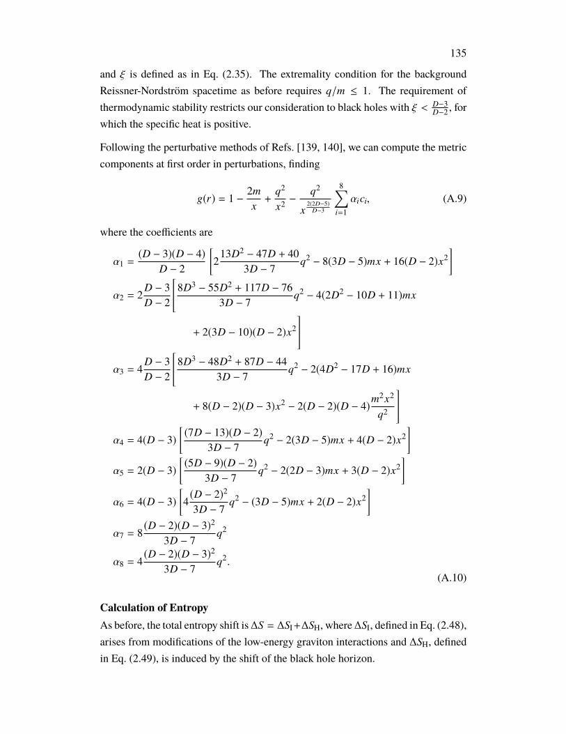
135

and ξ is defined as in Eq. (2.35). The extremality condition for the backgroundReissner-Nordström spacetime as before requires q/m ≤ 1. The requirement ofthermodynamic stability restricts our consideration to black holes with ξ < D−3

D−2 , forwhich the specific heat is positive.

Following the perturbative methods of Refs. [139, 140], we can compute the metriccomponents at first order in perturbations, finding

g(r) = 1 −2mx+

q2

x2 −q2

x2(2D−5)D−3

8∑i=1

αici, (A.9)

where the coefficients are

α1 =(D − 3)(D − 4)

D − 2

[2

13D2 − 47D + 403D − 7

q2 − 8(3D − 5)mx + 16(D − 2)x2]

α2 = 2D − 3D − 2

[8D3 − 55D2 + 117D − 76

3D − 7q2 − 4(2D2 − 10D + 11)mx

+ 2(3D − 10)(D − 2)x2

]α3 = 4

D − 3D − 2

[8D3 − 48D2 + 87D − 44

3D − 7q2 − 2(4D2 − 17D + 16)mx

+ 8(D − 2)(D − 3)x2 − 2(D − 2)(D − 4)m2x2

q2

]α4 = 4(D − 3)

[(7D − 13)(D − 2)

3D − 7q2 − 2(3D − 5)mx + 4(D − 2)x2

]α5 = 2(D − 3)

[(5D − 9)(D − 2)

3D − 7q2 − 2(2D − 3)mx + 3(D − 2)x2

]α6 = 4(D − 3)

[4(D − 2)2

3D − 7q2 − (3D − 5)mx + 2(D − 2)x2

]α7 = 8

(D − 2)(D − 3)2

3D − 7q2

α8 = 4(D − 2)(D − 3)2

3D − 7q2.

(A.10)

Calculation of EntropyAs before, the total entropy shift is∆S = ∆SI+∆SH, where∆SI, defined in Eq. (2.48),arises from modifications of the low-energy graviton interactions and ∆SH, definedin Eq. (2.49), is induced by the shift of the black hole horizon.

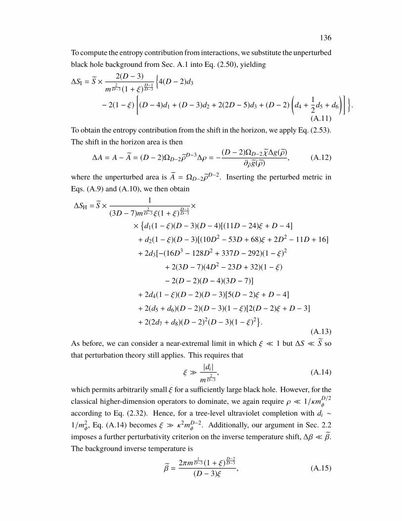
136

To compute the entropy contribution from interactions, we substitute the unperturbedblack hole background from Sec. A.1 into Eq. (2.50), yielding

∆SI = S ×2(D − 3)

m2

D−3 (1 + ξ)D−1D−3

4(D − 2)d3

− 2(1 − ξ)[(D − 4)d1 + (D − 3)d2 + 2(2D − 5)d3 + (D − 2)

(d4 +

12

d5 + d6

)] .

(A.11)To obtain the entropy contribution from the shift in the horizon, we apply Eq. (2.53).The shift in the horizon area is then

∆A = A − A = (D − 2)ΩD−2 ρD−3∆ρ = −

(D − 2)ΩD−2 χ∆g(ρ)

∂ρg(ρ), (A.12)

where the unperturbed area is A = ΩD−2 ρD−2. Inserting the perturbed metric in

Eqs. (A.9) and (A.10), we then obtain

∆SH = S ×1

(3D − 7)m 2D−3 ξ(1 + ξ)D−1

D−3×

×d1(1 − ξ)(D − 3)(D − 4)[(11D − 24)ξ + D − 4]

+ d2(1 − ξ)(D − 3)[(10D2 − 53D + 68)ξ + 2D2 − 11D + 16]

+ 2d3[−(16D3 − 128D2 + 337D − 292)(1 − ξ)2

+ 2(3D − 7)(4D2 − 23D + 32)(1 − ξ)

− 2(D − 2)(D − 4)(3D − 7)]

+ 2d4(1 − ξ)(D − 2)(D − 3)[5(D − 2)ξ + D − 4]

+ 2(d5 + d6)(D − 2)(D − 3)(1 − ξ)[2(D − 2)ξ + D − 3]

+ 2(2d7 + d8)(D − 2)2(D − 3)(1 − ξ)2.

(A.13)As before, we can consider a near-extremal limit in which ξ 1 but ∆S S sothat perturbation theory still applies. This requires that

ξ |di |

m2

D−3, (A.14)

which permits arbitrarily small ξ for a sufficiently large black hole. However, for theclassical higher-dimension operators to dominate, we again require ρ 1/κmD/2

φ

according to Eq. (2.32). Hence, for a tree-level ultraviolet completion with di ∼

1/m2φ, Eq. (A.14) becomes ξ κ2mD−2

φ . Additionally, our argument in Sec. 2.2imposes a further perturbativity criterion on the inverse temperature shift, ∆β β.The background inverse temperature is

β =2πm

1D−3 (1 + ξ)D−2

D−3

(D − 3)ξ, (A.15)

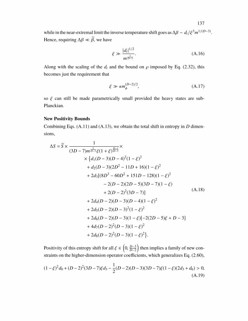
137

while in the near-extremal limit the inverse temperature shift goes as∆β ∼ di/ξ3m1/(D−3).

Hence, requiring ∆β β, we have

ξ |di |

1/2

m1

D−3. (A.16)

Along with the scaling of the di and the bound on ρ imposed by Eq. (2.32), thisbecomes just the requirement that

ξ κm(D−2)/2φ , (A.17)

so ξ can still be made parametrically small provided the heavy states are sub-Planckian.

New Positivity BoundsCombining Eqs. (A.11) and (A.13), we obtain the total shift in entropy in D dimen-sions,

∆S = S ×1

(3D − 7)m 2D−3 ξ(1 + ξ)D−1

D−3×

×d1(D − 3)(D − 4)2(1 − ξ)2

+ d2(D − 3)(2D2 − 11D + 16)(1 − ξ)2

+ 2d3[(8D3 − 60D2 + 151D − 128)(1 − ξ)2

− 2(D − 2)(2D − 5)(3D − 7)(1 − ξ)

+ 2(D − 2)2(3D − 7)]

+ 2d4(D − 2)(D − 3)(D − 4)(1 − ξ)2

+ 2d5(D − 2)(D − 3)2(1 − ξ)2

+ 2d6(D − 2)(D − 3)(1 − ξ)[−2(2D − 5)ξ + D − 3]

+ 4d7(D − 2)2(D − 3)(1 − ξ)2

+ 2d8(D − 2)2(D − 3)(1 − ξ)2.

(A.18)

Positivity of this entropy shift for all ξ ∈(0, D−3

D−2

)then implies a family of new con-

straints on the higher-dimension operator coefficients, which generalizes Eq. (2.60),

(1− ξ)2d0 + (D− 2)2(3D− 7)ξd3 −12(D− 2)(D− 3)(3D− 7)ξ(1− ξ)(2d3 + d6) > 0,

(A.19)

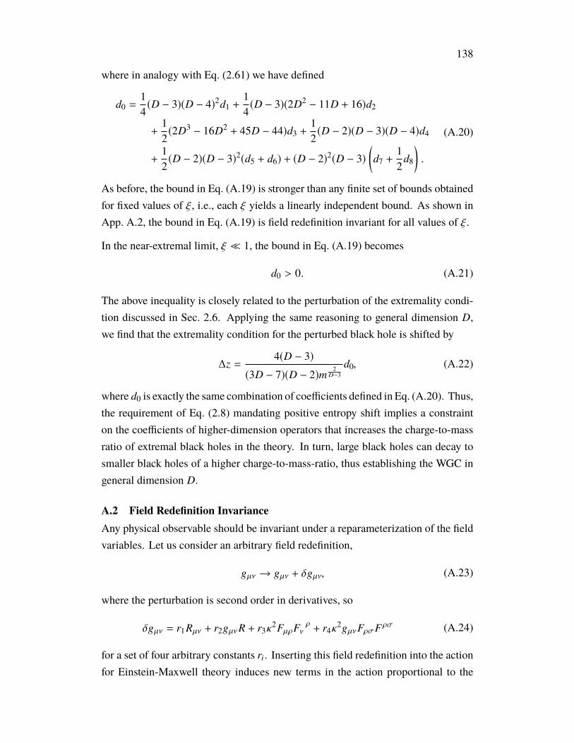
138

where in analogy with Eq. (2.61) we have defined

d0 =14(D − 3)(D − 4)2d1 +

14(D − 3)(2D2 − 11D + 16)d2

+12(2D3 − 16D2 + 45D − 44)d3 +

12(D − 2)(D − 3)(D − 4)d4

+12(D − 2)(D − 3)2(d5 + d6) + (D − 2)2(D − 3)

(d7 +

12

d8

).

(A.20)

As before, the bound in Eq. (A.19) is stronger than any finite set of bounds obtainedfor fixed values of ξ, i.e., each ξ yields a linearly independent bound. As shown inApp. A.2, the bound in Eq. (A.19) is field redefinition invariant for all values of ξ.

In the near-extremal limit, ξ 1, the bound in Eq. (A.19) becomes

d0 > 0. (A.21)

The above inequality is closely related to the perturbation of the extremality condi-tion discussed in Sec. 2.6. Applying the same reasoning to general dimension D,we find that the extremality condition for the perturbed black hole is shifted by

∆z =4(D − 3)

(3D − 7)(D − 2)m 2D−3

d0, (A.22)

where d0 is exactly the same combination of coefficients defined in Eq. (A.20). Thus,the requirement of Eq. (2.8) mandating positive entropy shift implies a constrainton the coefficients of higher-dimension operators that increases the charge-to-massratio of extremal black holes in the theory. In turn, large black holes can decay tosmaller black holes of a higher charge-to-mass-ratio, thus establishing the WGC ingeneral dimension D.

A.2 Field Redefinition InvarianceAny physical observable should be invariant under a reparameterization of the fieldvariables. Let us consider an arbitrary field redefinition,

gµν → gµν + δgµν, (A.23)

where the perturbation is second order in derivatives, so

δgµν = r1Rµν + r2gµνR + r3κ2FµρF ρ

ν + r4κ2gµνFρσFρσ (A.24)

for a set of four arbitrary constants ri. Inserting this field redefinition into the actionfor Einstein-Maxwell theory induces new terms in the action proportional to the

139

equations of motion,1

δL =1

2κ2 δgµν

(Rµν −

12

Rgµν − κ2Tµν

). (A.25)

This has the net effect of shifting the higher-dimension operator coefficients in theaction by

d1 → d1 −14

r1 −D − 2

4r2

d2 → d2 +12

r1

d3 → d3

d4 → d4 +18

r1 +D − 4

8r2 −

14

r3 −D − 2

4r4

d5 → d5 −12

r1 +12

r3

d6 → d6

d7 → d7 +18

r3 +D − 4

8r4

d8 → d8 −12

r3.

(A.26)

Because the field redefinition depends on four arbitrary constants, this reduces thenaive basis of eight higher-dimension operator coefficients down to a set of fourcombinations that are automatically field redefinition invariant:

d0, d3, d6, d9, (A.27)

where d0 is defined in Eq. (A.20) and d9 = d2 + d5 + d8. All physical quantities,like the bounds in Eqs. (2.60) and (A.19), depend only on these combinations ofcoefficients.

1The particular field redefinition in which the pure Einstein-Maxwell equations of motion aresubstituted into the higher-dimension operators is a special case of the transformation in Eq. (A.24).

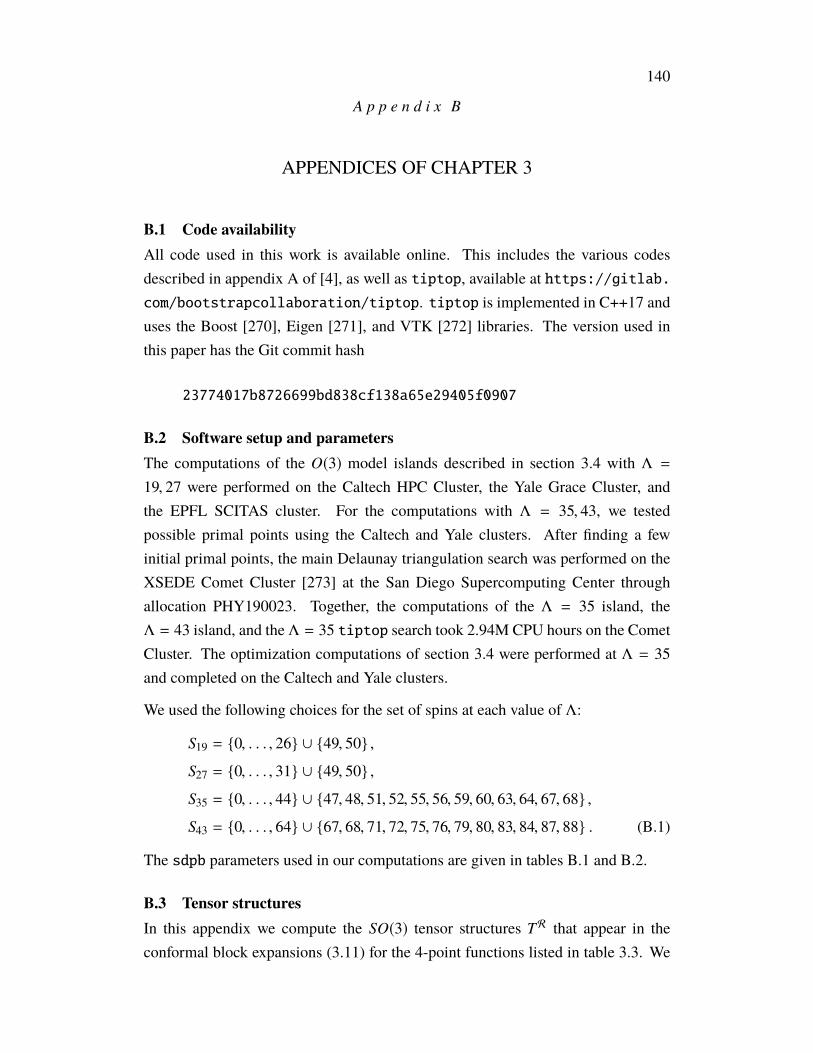
140

A p p e n d i x B

APPENDICES OF CHAPTER 3

B.1 Code availabilityAll code used in this work is available online. This includes the various codesdescribed in appendix A of [4], as well as tiptop, available at https://gitlab.com/bootstrapcollaboration/tiptop. tiptop is implemented in C++17 anduses the Boost [270], Eigen [271], and VTK [272] libraries. The version used inthis paper has the Git commit hash

23774017b8726699bd838cf138a65e29405f0907

B.2 Software setup and parametersThe computations of the O(3) model islands described in section 3.4 with Λ =19, 27 were performed on the Caltech HPC Cluster, the Yale Grace Cluster, andthe EPFL SCITAS cluster. For the computations with Λ = 35, 43, we testedpossible primal points using the Caltech and Yale clusters. After finding a fewinitial primal points, the main Delaunay triangulation search was performed on theXSEDE Comet Cluster [273] at the San Diego Supercomputing Center throughallocation PHY190023. Together, the computations of the Λ = 35 island, theΛ = 43 island, and the Λ = 35 tiptop search took 2.94M CPU hours on the CometCluster. The optimization computations of section 3.4 were performed at Λ = 35and completed on the Caltech and Yale clusters.

We used the following choices for the set of spins at each value of Λ:

S19 = 0, . . . , 26 ∪ 49, 50 ,

S27 = 0, . . . , 31 ∪ 49, 50 ,

S35 = 0, . . . , 44 ∪ 47, 48, 51, 52, 55, 56, 59, 60, 63, 64, 67, 68 ,

S43 = 0, . . . , 64 ∪ 67, 68, 71, 72, 75, 76, 79, 80, 83, 84, 87, 88 . (B.1)

The sdpb parameters used in our computations are given in tables B.1 and B.2.

B.3 Tensor structuresIn this appendix we compute the SO(3) tensor structures TR that appear in theconformal block expansions (3.11) for the 4-point functions listed in table 3.3. We

141

Λ 19 27 35 43keptPoleOrder 14 14 32 40

order 60 60 80 90spins S19 S27 S35 S43

precision 768 768 960 1024dualityGapThreshold 10−30 10−30 10−30 10−75

primalErrorThreshold 10−200 10−200 10−200 10−200

dualErrorThreshold 10−200 10−200 10−200 10−200

initialMatrixScalePrimal 1040 1050 1050 1060

initialMatrixScaleDual 1040 1050 1050 1060

feasibleCenteringParameter 0.1 0.1 0.1 0.1infeasibleCenteringParameter 0.3 0.3 0.3 0.3

stepLengthReduction 0.7 0.7 0.7 0.7maxComplementarity 10100 10130 10160 10200

Table B.1: Parameters used for the computations of the conformal bootstrap islandsin section 3.4. The sets SΛ are defined in (B.1).

Λ 35keptPoleOrder 30

order 60spins S35

precision 768dualityGapThreshold 10−20

primalErrorThreshold 10−50

dualErrorThreshold 10−60

initialMatrixScalePrimal 1050

initialMatrixScaleDual 1050

feasibleCenteringParameter 0.1infeasibleCenteringParameter 0.3

stepLengthReduction 0.7maxComplementarity 10160

Table B.2: Parameters used for the optimization computations in section 3.4. Theset S35 is defined in (B.1).

142

start by defining a basis of tensors for each configuration in table 3.3:

BIφφφφ =

©­­«δi jδkl

δikδ jl

δilδ j k

ª®®®¬ ,

BItttt =

©­­­­­­­«

δi1 j1δi2 j2δk1l1δk2l2

δi1k1δi2k2δ j1l1δ j2l2

δi1l1δi2l2δk1 j1δk2 j2

δi1 j1δi2k2δk1l1δ j2l2

δi1 j1δi2l1δ j2k1δk2l2

ª®®®®®®®®¬,

BItφtφ =

©­­«δi1k1δi2k2δ j1l1

δi1 j1δi2k2δk1l1

δi1l1δi2k2δ j1k1

ª®®®¬ ,BI

ttφφ =©­­«δi1 j1δi2 j2δk1l1

δi1k1δi2 j2δ j1l1

δi1l1δi2 j2δk1 j1

ª®®®¬ ,Bssss = 1 ,

Bφsφs = δik ,

Btsts = δi1k1δi2k2 ,

Bttss = δi1 j1δi2 j2 ,

Bφφss = δi j ,

Bφsφt = δil1δkl2 ,

Bφφst = δil1δ jl2 ,

Bsttt = δ j1k1δ j2l1δk2l2 ,

(B.2)

where the indices for each of the four operators are labeled as i, j, k, l respectively,all indices with the same letter should be symmetrized with the trace removed,and for simplicity we suppress the indices on the left-hand side. For the first fourconfigurations with non-trivial bases, we can find the tensor structure using the rank-2 SO(3) Casimir C acting on a basis B with n,m number of i, j indices, respectively,as:

CBI =∑

J

M I J BJ , C ≡ (Gi1i′1⊕ · · · ⊕ Gin

i′n⊕ G j1

j ′1⊕ · · · ⊕ G jm

j ′m)2 , (B.3)

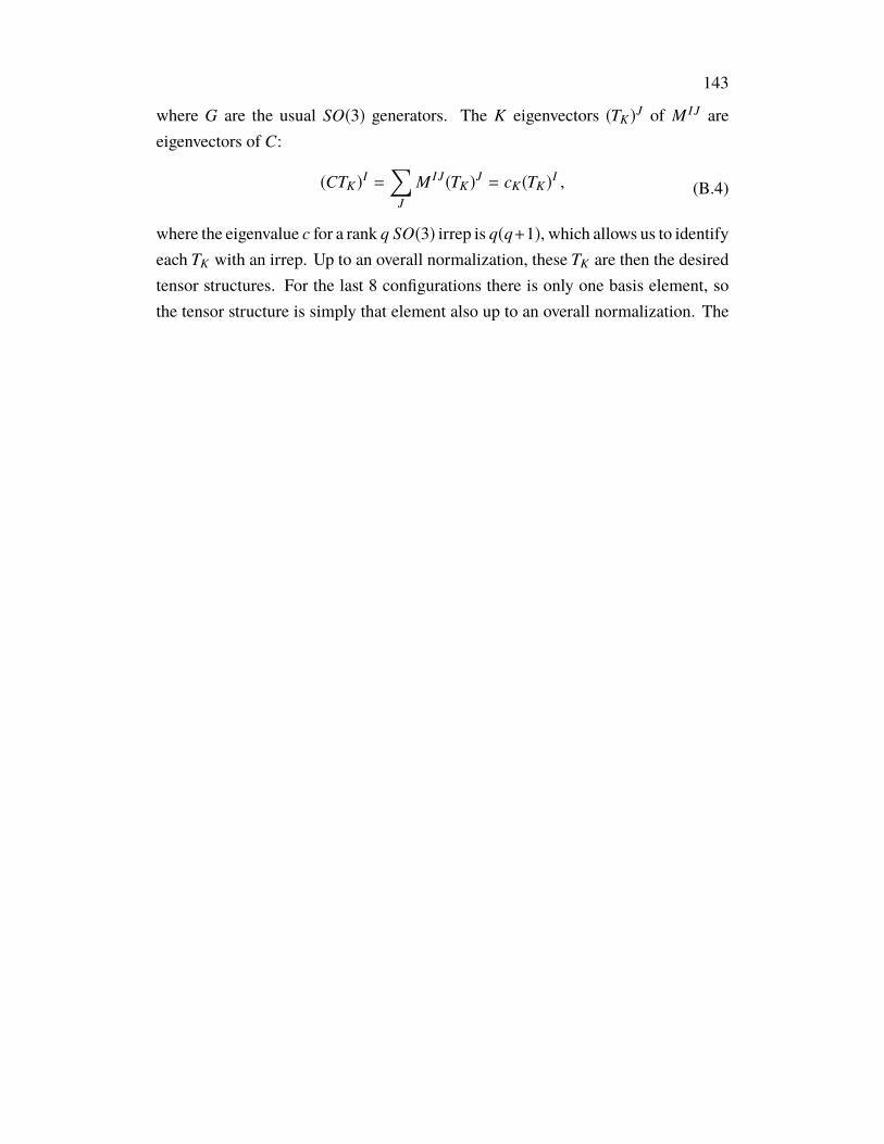
143

where G are the usual SO(3) generators. The K eigenvectors (TK)J of M I J are

eigenvectors of C:

(CTK)I =

∑J

M I J(TK)J = cK(TK)

I , (B.4)

where the eigenvalue c for a rank q SO(3) irrep is q(q+1), which allows us to identifyeach TK with an irrep. Up to an overall normalization, these TK are then the desiredtensor structures. For the last 8 configurations there is only one basis element, sothe tensor structure is simply that element also up to an overall normalization. The

144

final list of tensor structures is then

〈φφφφ〉 : T0+1−1−1−1− = B1

φφφφ ,

T1+1−1−1−1− = B2

φφφφ − B3φφφφ ,

T2+1−1−1−1− = B2

φφφφ + B3φφφφ −

23

B1φφφφ ,

〈tttt〉 : T0+2+2+2+2+ = B1

tttt ,

T1+2+2+2+2+ = B4

tttt − B5tttt ,

T2+2+2+2+2+ = B4

tttt + B5tttt −

23

B1tttt ,

T3+2+2+2+2+ = B5

tttt − B4tttt −

54

B3tttt +

54

B2tttt ,

T4+2+2+2+2+ = −B5

tttt − B4tttt +

712

B3tttt +

712

B2tttt +

1330

B1tttt ,

〈tφtφ〉, 〈φttφ〉 : T1−2+1−2+1− = 2B2

tφtφ ,

T2−2+1−2+1− = −4B1

tφtφ + 2B2tφtφ + 4B3

tφtφ ,

T3−2+1−2+1− = 10B1

tφtφ − 8B2tφtφ + 20B3

tφtφ ,

〈ttφφ〉 : T0+2+2+1−1− = B1

ttφφ ,

T1+2+2+1−1− = B2

ttφφ − B3ttφφ ,

T2+2+2+1−1− = B2

ttφφ + B3ttφφ −

23

B1ttφφ ,

〈ssss〉 : T0+0+0+0+0+ = Bssss ,

〈φsφs〉, 〈sφφs〉 : T1−1−0+1−2+ = Bφsφs ,

〈tsts〉, 〈stts〉 : T2+2+0+2+0+ = Btsts ,

〈ttss〉 : T0+2+2+0+0+ = Bttss ,

〈φφss〉 : T0+1−1−0+0+ = Bφφss ,

〈φsφt〉, 〈sφφt〉 : T1−1−0+1−2+ =

√2Bφsφt ,

〈φφst〉 : T2+1−1−0+2+ =

√2Bφφst ,

〈sttt〉, 〈ttst〉 : T2+0+2+2+2+ =

√2Bsttt .

(B.5)

The overall normalization of these tensor structures has been chosen so that the OPEcoefficients λϕ1ϕ2O and λϕ3ϕ4O in (3.11) are consistent under permutation of theirsubscripts. This can be checked using the free theory, where we have the operators

s(x) ≡1√

6φi(x)φi(x) , ti j(x) ≡

1√

2φi(x)φ j(x) − trace , (B.6)

145

which have been normalized consistent with the 2-point function normalization in(3.13). We can then compute all the 4-point functions in table 3.3 using Wickcontractions and expand in blocks as in (3.11) using the tensor structures in (B.5) toverify this consistency.1

B.4 Computed pointsIn table B.3 we list the 38 primal points we have computed in the Λ = 43 island andin table B.4 we list the 270 dual points we computed at Λ = 43. In table B.5 we listthe 7 primal points we use for the optimization computations described in section3.4.

In Figure B.1 we show a plot of the allowed regions at Λ = 19, 27, 35, 43 after per-forming an affine transformation which makes the Λ = 19 region roughly spherical.The precise affine transformation is given by

x = 228.67 − 107.177∆s − 43.8661∆t − 8.77302∆φ ,

y = −1061.39 − 694.406∆s + 1612.44∆t + 420.885∆φ , (B.8)

z = 2590.87 − 221.685∆s + 2629.52∆t − 10439.6∆φ .

1Note that there is another convention generated by the package autoboot [189]. Our resultsfor scanned external OPEs are different from the autoboot (ab) convention by(

λussss, λ

ustts, λ

usφφt, λ

usφφs, λ

usttt

)=

(λabsss,

1√

3λabtts,

1√

5λabφφt,

1√

10λabφφs,

√635λabttt

). (B.7)

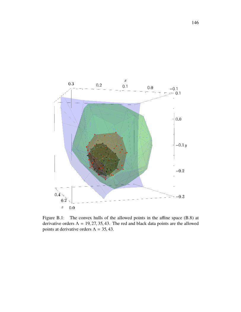
146

Figure B.1: The convex hulls of the allowed points in the affine space (B.8) atderivative orders Λ = 19, 27, 35, 43. The red and black data points are the allowedpoints at derivative orders Λ = 35, 43.

147

∆φ ∆s ∆tλsssλφφs

λt t sλφφs

λφφtλφφs

λt t tλφφs

0.5189783882 1.5953612741 1.2097311776 0.9658557781 1.8764272526 1.6683150562 2.86082802950.5189583670 1.5949959168 1.2096121876 0.9637866930 1.8759071995 1.6681321958 2.86040109330.5189461401 1.5949711389 1.2095536502 0.9650503920 1.8758868056 1.6680723076 2.86019766930.5189272852 1.5948074081 1.2094888929 0.9652812111 1.8758487781 1.6680235398 2.86030616750.5189613339 1.5952564268 1.2096662222 0.9662461846 1.8763712143 1.6682528867 2.86074752470.5189198114 1.5946719225 1.2094285955 0.9639220579 1.8755694851 1.6679344313 2.85994095710.5189172850 1.5946165394 1.2094312995 0.9634877179 1.8756194443 1.6679524398 2.85998353290.5189500473 1.5951798121 1.2096307308 0.9661780974 1.8763286685 1.6682360908 2.86072673820.5189649901 1.5951958587 1.2096821376 0.9647455098 1.8763265571 1.6682560921 2.86083858870.5189431822 1.5950799657 1.2095793546 0.9658559545 1.8761787760 1.6681550694 2.86040664340.5189526027 1.5949370220 1.2096034154 0.9633651701 1.8758925982 1.6681462865 2.86055689490.5189301757 1.5949315300 1.2095370407 0.9653175705 1.8761152596 1.6681181238 2.86058167300.5189168372 1.5946844827 1.2094296026 0.9642949506 1.8756631385 1.6679573604 2.85994183240.5189483062 1.5950509260 1.2095711164 0.9654214538 1.8760347497 1.6681115766 2.86025824140.5189153515 1.5946825124 1.2094352034 0.9643765341 1.8757126829 1.6679642216 2.86010680050.5189440155 1.5949715807 1.2095885922 0.9644538043 1.8760784038 1.6681817119 2.86073650300.5189150284 1.5945099455 1.2094139921 0.9622684128 1.8754680443 1.6679176085 2.85992904310.5189347282 1.5947841912 1.2094914029 0.9639498317 1.8756547299 1.6679896459 2.85998296500.5189802791 1.5952998277 1.2097251950 0.9649312284 1.8762516023 1.6682831892 2.86091055110.5189248611 1.5948368279 1.2094835818 0.9649249785 1.8759055628 1.6680304724 2.86008998460.5189306747 1.5946954535 1.2094799696 0.9630209667 1.8756016368 1.6679818979 2.86005563640.5189217812 1.5947698290 1.2094894198 0.9646493947 1.8759369337 1.6680732162 2.86036823820.5189121284 1.5945494559 1.2093932170 0.9632128469 1.8754599512 1.6678971836 2.85972950690.5189738261 1.5953116389 1.2096932265 0.9658322350 1.8762663003 1.6682491526 2.86062772060.5189145348 1.5947341024 1.2094532479 0.9650247104 1.8759430722 1.6680183536 2.86024023870.5189014384 1.5944048949 1.2093555400 0.9627737264 1.8753951336 1.6678520403 2.85979520500.5189305457 1.5947604700 1.2094652572 0.9640748832 1.8756103384 1.6679623986 2.85988099640.5189623990 1.5950949062 1.2096629593 0.9640070854 1.8761554772 1.6682313428 2.86081895530.5189460789 1.5950582403 1.2095808918 0.9654253734 1.8761261589 1.6681362224 2.86050451350.5189301505 1.5949452685 1.2095278745 0.9657542568 1.8760854806 1.6681017321 2.86049623270.5189685635 1.5953320391 1.2097096529 0.9660028358 1.8764583565 1.6683135549 2.86095751170.5189497511 1.5949209137 1.2095606097 0.9638109344 1.8758202300 1.6680711351 2.86018998220.5189337664 1.5947155621 1.2095107201 0.9623655424 1.8757184969 1.6680386790 2.86024502230.5189453714 1.5951023898 1.2096147301 0.9659065454 1.8763651079 1.6682206940 2.86079195210.5189862601 1.5954028918 1.2097515683 0.9654844905 1.8763339257 1.6683105873 2.86078814510.5189476979 1.5949533896 1.2096010827 0.9637175659 1.8760304271 1.6681861098 2.86067295850.5189346015 1.5950348003 1.2095678602 0.9659534043 1.8763062992 1.6681684361 2.86062481900.5189598320 1.5951484795 1.2096664021 0.9647455098 1.8763265571 1.6682560921 2.8608385887

Table B.3: Allowed points in the Λ = 43 island.

148

∆φ ∆s ∆t

0.5187966798 1.5921850401 1.20862288040.5189025751 1.5940361780 1.20929594080.5189114364 1.5946504985 1.20938724620.5189189599 1.5941920882 1.20932997410.5189288736 1.5938535802 1.20910785060.5186945881 1.5924442671 1.20842458650.5187373587 1.5921586352 1.20843127430.5187762022 1.5918820333 1.20865468050.5187826937 1.5914255278 1.20853106410.5188353864 1.5934222782 1.20900202490.5188362222 1.5935429810 1.20898183860.5188416799 1.5933781659 1.20894818690.5188478354 1.5938857812 1.20913628790.5188535569 1.5932852248 1.20882140420.5188541349 1.5932916366 1.20896522720.5188547707 1.5939362783 1.20903124210.5188571369 1.5930390946 1.20905696470.5188574085 1.5927203987 1.20899176990.5188612075 1.5939110280 1.20914557400.5188615055 1.5937167137 1.20909098980.5188768144 1.5938159784 1.20902162350.5188830465 1.5941282784 1.20924435330.5188846453 1.5942465723 1.20925893870.5188859294 1.5941864473 1.20927616620.5188862012 1.5941115729 1.20922550650.5188873828 1.5941812791 1.20925061610.5188874108 1.5939452740 1.20918599610.5188875107 1.5943066473 1.20930070220.5188888052 1.5938613363 1.20921212330.5188955343 1.5940894591 1.20921275670.5188965815 1.5941441764 1.20929750810.5189023610 1.5945285422 1.20938340190.5189038211 1.5934538031 1.20907008920.5189054986 1.5948072619 1.20945760260.5189068088 1.5944337603 1.20929096330.5189083086 1.5946728229 1.20941314890.5189105727 1.5946476632 1.20944864450.5189114164 1.5934097919 1.20914146520.5189153608 1.5942042741 1.20929824920.5189179786 1.5948735383 1.20949800560.5189191601 1.5945565549 1.20946403680.5189241090 1.5941509824 1.20940027830.5189333103 1.5939599259 1.20945232970.5189333930 1.5943501521 1.20942324630.5189346097 1.5944851028 1.20957407160.5189237305 1.5944279251 1.20939053910.5188043639 1.5926034786 1.20879056250.5188819788 1.5940503654 1.20916640500.5189348544 1.5939659673 1.20936059050.5189331311 1.5945586909 1.20948613730.5188609431 1.5938359757 1.20911383920.5189041783 1.5931200581 1.20913594610.5189211553 1.5940068208 1.20937119760.5188230608 1.5930667503 1.20878330970.5187918880 1.5920291631 1.20865566370.5187954081 1.5933857238 1.20887227120.5188120708 1.5921939042 1.20854756220.5188685720 1.5940780889 1.20922002130.5188737587 1.5938867482 1.20912821020.5188791085 1.5939475441 1.20922698430.5188860122 1.5944086593 1.20931181420.5188881256 1.5943425103 1.20926060770.5188962192 1.5944000610 1.20930369260.5188995836 1.5944714851 1.20934799090.5189042967 1.5942997732 1.20934508740.5189061160 1.5944245329 1.20930548110.5189130711 1.5943416289 1.20929388870.5189282439 1.5948696505 1.20943544950.5189381636 1.5945869176 1.20953732900.5189209582 1.5946145623 1.20939710260.5188528255 1.5932931016 1.20886476490.5188758367 1.5937600844 1.20906942060.5189034036 1.5943173907 1.20927537860.5187933545 1.5923524886 1.20858510520.5188028340 1.5925358527 1.20861819250.5188672706 1.5938859690 1.20907849020.5188721453 1.5939744974 1.20921140190.5188815521 1.5940429270 1.20902309250.5188876803 1.5938597752 1.20924397370.5188893843 1.5942285412 1.20924300030.5188959297 1.5932555635 1.20926138680.5189185378 1.5944533142 1.20938993620.5189206686 1.5947871150 1.20945293100.5189513139 1.5946586522 1.20945234240.5189385685 1.5946849443 1.20946035450.5189444575 1.5946106034 1.20944269440.5189597959 1.5951033035 1.20956848290.5190271291 1.5953552765 1.20993200470.5191718508 1.5977020194 1.21054678900.5189415400 1.5950976756 1.2095440010

∆φ ∆s ∆t

0.5189424979 1.5947703013 1.20936017230.5189461102 1.5944802637 1.20954171290.5189461142 1.5952505758 1.20961138110.5189509729 1.5951396676 1.20966080870.5189524992 1.5951035671 1.20957336500.5189561892 1.5950657026 1.20965309410.5189575751 1.5955030599 1.20964013270.5189576562 1.5952623581 1.20968515500.5189595475 1.5954833608 1.20971489700.5189682325 1.5951956784 1.20963214720.5189696503 1.5942534718 1.20936178780.5189733687 1.5949010519 1.20957860600.5189772029 1.5950953535 1.20964404130.5189800482 1.5949290496 1.20970355400.5189804744 1.5953372481 1.20978753280.5189818184 1.5960483373 1.20987118940.5189830613 1.5952764767 1.20981757290.5189871624 1.5963425034 1.20989152610.5189966010 1.5956243058 1.20985895010.5190066292 1.5959897652 1.20994810840.5190086343 1.5954797940 1.20988726900.5190093925 1.5948495201 1.20953110730.5190140405 1.5954232716 1.20988879550.5190158019 1.5958546312 1.20988000290.5190176624 1.5957396035 1.20995248000.5190182636 1.5952950369 1.20971976300.5190222887 1.5962382824 1.21004065990.5190294335 1.5944921267 1.20973865080.5190368914 1.5960448579 1.20995405430.5190379431 1.5958717009 1.20996550300.5190482917 1.5959534075 1.20996698690.5190587928 1.5959983074 1.21001696450.5190598740 1.5957892478 1.21000802160.5190647361 1.5962663027 1.21015213450.5190695509 1.5960823090 1.21013503230.5190725277 1.5960088046 1.21009912030.5190732657 1.5962258325 1.21007445100.5190787856 1.5961544869 1.21011999500.5190839387 1.5962931060 1.21018344890.5190846538 1.5964564464 1.21018238240.5190882951 1.5952923328 1.20994882380.5191014483 1.5962764902 1.21024336120.5191200121 1.5963878404 1.21042546920.5191238375 1.5961605267 1.21009604570.5191427139 1.5977670021 1.21068789670.5191456549 1.5971361619 1.21053086420.5191695884 1.5970766016 1.21065950540.5191747564 1.5961581015 1.21041659380.5191752118 1.5973305922 1.21048273290.5191772163 1.5979425702 1.21078345420.5191998406 1.5976763974 1.21083433700.5192110760 1.5974046747 1.21057844280.5192313582 1.5976397828 1.21091349290.5192577054 1.5985007420 1.21106022700.5192609179 1.5973050662 1.21087249940.5192751871 1.5986516951 1.21116932130.5193182009 1.5988546582 1.21128326240.5193313395 1.5984303509 1.21115333120.5193414850 1.5980461969 1.21115691210.5193551983 1.5998541317 1.21156975950.5193848130 1.5991038253 1.21149731350.5193945892 1.5989679837 1.21142172210.5190798632 1.5964346557 1.21020617910.5189741917 1.5955685395 1.20976977150.5189927891 1.5951952177 1.20973727910.5189996154 1.5950788378 1.20970541130.5190167890 1.5955602397 1.20988737870.5190308122 1.5949198011 1.20963898440.5190339170 1.5955996031 1.20987491370.5190412371 1.5962115376 1.21006811240.5191177942 1.5966893312 1.21031479620.5192445379 1.5985977149 1.21102827280.5192695593 1.5991098729 1.21125864080.5193036599 1.5986614215 1.21132797310.5192414561 1.5971357017 1.21063547010.5189651659 1.5950121240 1.20966679880.5191751265 1.5980350400 1.21073878660.5189584563 1.5953669776 1.20969547530.5189653470 1.5950297999 1.20969048320.5189699612 1.5955018495 1.20973422110.5189780238 1.5954734077 1.20970718120.5189801701 1.5956399491 1.20981955240.5189846429 1.5956222286 1.20980437390.5189848116 1.5942072297 1.20943161010.5189955714 1.5956904175 1.20986019020.5189970055 1.5958004005 1.20983159600.5190050996 1.5957883004 1.20988656960.5190163339 1.5957550559 1.20991835380.5190199557 1.5956651380 1.20992952960.5190607004 1.5962908080 1.2100873837

∆φ ∆s ∆t

0.5190663597 1.5958743309 1.21009570550.5190718073 1.5963854342 1.21015431030.5191015148 1.5964779979 1.21031739130.5191201873 1.5971879432 1.21035573290.5191327281 1.5966479322 1.21021573570.5192390608 1.5990575125 1.21111650180.5189384637 1.5945786868 1.20929646120.5189388374 1.5949295375 1.20948865180.5189406470 1.5951736959 1.20960255780.5189435236 1.5946628177 1.20950795680.5189591857 1.5937291370 1.20944790430.5189690300 1.5947953102 1.20957001390.5189782490 1.5955014573 1.20973945180.5189785861 1.5948000056 1.20962176020.5189943897 1.5951836165 1.20967268790.5190020000 1.5955721180 1.20986149480.5190031045 1.5956425756 1.20982937070.5190089551 1.5959677551 1.20994138220.5190264203 1.5960422185 1.21001908360.5190349642 1.5958180205 1.20997065580.5190621203 1.5957337543 1.20983892820.5191180161 1.5968444953 1.21034562800.5191470052 1.5962315204 1.21045716130.5191921249 1.5963777247 1.21059755450.5192666256 1.5975999519 1.21097690540.5192834446 1.5981834807 1.21094786780.5192153931 1.5971409678 1.21086191230.5190126129 1.5960328832 1.20984118200.5189956968 1.5952697384 1.20978913450.5190907117 1.5964405597 1.21025644680.5189972378 1.5954623091 1.20972882490.5192342602 1.5977739085 1.21067884120.5192967458 1.5978374167 1.21096549580.5190531962 1.5957547434 1.21002534870.5190597017 1.5959435763 1.21009608080.5189393710 1.5943081218 1.20945180820.5189538314 1.5947940605 1.20948962800.5189547388 1.5948394180 1.20955850360.5189639253 1.5945186785 1.20947253810.5189836057 1.5957551038 1.20982195260.5189905121 1.5953498417 1.20980071940.5189919017 1.5941900169 1.20952883100.5189979105 1.5956955072 1.20977960400.5189995667 1.5957402879 1.20990582160.5190123754 1.5941042932 1.20953907730.5190157406 1.5958569876 1.20992005450.5190278431 1.5965081852 1.21002810150.5190325131 1.5959081051 1.20996965380.5190520384 1.5963152404 1.21008412770.5190588609 1.5960509826 1.20990905480.5190715439 1.5955912797 1.21014975260.5190926525 1.5965090465 1.21024035190.5191170800 1.5974916154 1.21050643350.5191778676 1.5977308111 1.21078439230.5192544590 1.5971285489 1.21077464400.5192666631 1.5983714488 1.21093568230.5192812420 1.5987160882 1.21111015810.5193040795 1.5983604351 1.21120104790.5189685870 1.5947440353 1.20955469730.5189469362 1.5948003211 1.20945698960.5190500327 1.5959140301 1.21006738440.5190853457 1.5968203648 1.21033566460.5189402432 1.5947339426 1.20951325720.5189866072 1.5952602047 1.20973864610.5189466850 1.5949712041 1.20954392760.5189977538 1.5955819151 1.20981876860.5189417109 1.5948151822 1.20951162420.5189887395 1.5955311410 1.20979987380.5189805152 1.5954860043 1.20975745710.5189068037 1.5944354150 1.20936313400.5189664963 1.5953900793 1.20970888700.5189046136 1.5944739467 1.20934983900.5189477115 1.5951943364 1.20961437060.5189476015 1.5951048660 1.20958571350.5189392465 1.5947339121 1.20952578800.5189758138 1.5951810417 1.20971319020.5189281878 1.5946813688 1.20949968500.5189741332 1.5953607762 1.20974178470.5189225607 1.5945597787 1.20943807660.5189250556 1.5947901155 1.20945997230.5189931813 1.5954181855 1.20976908330.5189417323 1.5950007532 1.20953632690.5189436065 1.5950358588 1.20960599390.5189964571 1.5954554607 1.20980054010.5189717084 1.5953355582 1.20968327960.5189194848 1.5945704303 1.20941298250.5189261393 1.5947676104 1.20950658540.5189163665 1.5945874291 1.20938992780.5188888691 1.5942500939 1.20928591430.5189931888 1.5954995182 1.2097983737

Table B.4: Disallowed points computed at Λ = 43.

∆φ ∆s ∆tλsssλφφs

λt t sλφφs

λφφtλφφs

λt t tλφφs

∆T ′ − ∆T ∆J′ − ∆J

0.5189121284 1.594549456 1.209393217 0.9632128469 1.875459951 1.667897184 2.859729507 1.0 0.10.5189145348 1.594734102 1.209453248 0.9650247103 1.875943072 1.668018354 2.860240239 1.0 1.00.5189337664 1.594715562 1.209510720 0.9623655424 1.875718497 1.668038679 2.860245022 1.0 1.00.5189415373 1.594941048 1.209557043 0.9646177852 1.875978443 1.668107872 2.860397307 1.0 1.00.5189431822 1.595079966 1.209579355 0.9658559545 1.876178776 1.668155069 2.860406643 1.0 0.10.5189685635 1.595332039 1.209709653 0.9660028358 1.876458357 1.668313555 2.860957512 1.0 0.10.5189862601 1.595402892 1.209751568 0.9654844905 1.876333926 1.668310587 2.860788145 1.0 0.1

Table B.5: Allowed points in the Λ = 43 island used to obtain bounds on λφφs, CT ,and CJ , along with the gaps above ∆T and ∆J that were assumed.

149

A p p e n d i x C

APPENDICES OF CHAPTER 4

C.1 Infinite MPSIn the main text, we define a Matrix Product State on a finite number of sites withopen boundary conditions. To represent the true and false vacua of a spin chain, weuse infinite MPS (iMPS), in which the number of sites→∞

|ψ〉 =∑s

v†L . . . A(s−1)−1 A(s0)

0 A(s1)1 . . . vR | . . . s−1s0s1 . . . 〉, (C.1)

where A(s)j is a D j−1 × D j matrix assigned to site j in basis-state s and vL and vR

are appropriately-sized boundary vectors. In a uniform (translation invariant) iMPS,we use the same tensor A everywhere: A(s)j = A(s) ∀ j ∈ Z. Such a state has a welldefined norm for generic choices of vL and vR if the D2 × D2 "transfer matrix”

𝐴*

𝐴=

∑s

A(s) ⊗ A(s)∗, (C.2)

where ∗ indicates the complex conjugate has a nondegenerate eigenvalue of largestmagnitude, with A normalized so that this eigenvalue is equal to 1 [234]. Thiscondition implies exponential decay of correlations with distance. By additionallynormalizing vL and vR appropriately, we can achieve 〈ψ |ψ〉 = 1. The precisechoice of boundary vectors does not affect bulk expectation values due to theaforementioned exponential decay of correlators.

Nonuniform windowsTo build the bubble states of the main text, and to simulate their evolution in time,we allow the tensors of an otherwise uniform iMPS to vary within a "window”,consisting of N contiguous sites. These states have the form

|ψ〉 =∑s

| . . . s1 . . . sN . . . 〉×v†

L

( 0∏i=−∞

A(si)L

)A(s1)

1 . . . A(sN )N©­«∞∏

j=N+1A(sj )R

ª®¬ vR, (C.3)

where AL and AR parameterize the semi-infinite left and right bulk parts of thechain and A1 . . . AN parameterize the nonuniform window. The above transfer-matrix conditions for a well-defined uniform iMPS must be satisfied for both the

150

AL and AR tensors. The norm of the state is then determined by the content of thewindow tensors A1 . . . AN . For the bubble states, we let AL = AR = , whereis the tensor optimized for the uniform ground state (true vacuum) of the spin chain.We then choose A1 . . . AN to represent a false-vacuum bubble, as described belowin App. C.3. For example, a fully localized bubble state (the kink-antikink state ofFig. 4.4) has A1 = (representing a kink), A2 . . . AN−1 = (representing thefalse vacuum), and AN = (representing the antikink).

C.2 Finding the true and false vacuaFinding the true vacuumThe tensor A defining a uniform iMPS (C.1) can be optimized to represent low-energy, translation-invariant states of gapped quantum spin chains using variousalgorithms. We use the nonlinear conjugate-gradient method described in [207] andimplemented in the evoMPS package [264] to find a uniform iMPS that approxi-mately describe the ground states of gapped quantum spin chains. We denote theoptimized iMPS tensor .

Finding the false vacuumWe explain how we obtain an iMPS representation of the false vacuum in practicein App. C.2 below. In this section, we consider the nature of the false vacuum moregenerally.

For the broken Z2 symmetry of the Ising-like chain in the main text, the false vacuum|Ω〉 is a state that has opposite spin orientation to the true vacuum |Ω〉. It should alsobe like a vacuum, in that it should be a spatially uniform, approximately static statenear a local energetic minimum with respect to some constraint, such as locality.

A candidate state is the "flipped” vacuum(∏j

X j

)|Ω〉. (C.4)

It is spatially uniform and typically close to an energetic minimum in the followingsense: If we apply a finite string

∏Lj=1 X j of length L, the change in energy will be

positive for small values of L, becoming negative only after the O(2hL) energy lostby replacing false vacuumwith true vacuum on L sites is larger than the O(1) energypenalty of spin anti-alignment at the boundaries. However, the flipped vacuum isgenerally not close to being an eigenstate in case of a nonzero symmetry-breakingfield parameter h and therefore is not suitably static. Nevertheless, one might begin

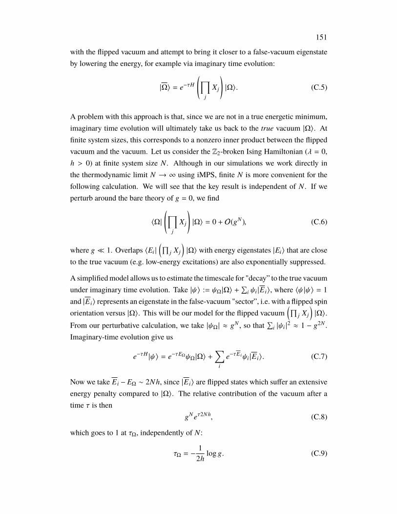
151

with the flipped vacuum and attempt to bring it closer to a false-vacuum eigenstateby lowering the energy, for example via imaginary time evolution:

|Ω〉 = e−τH

(∏j

X j

)|Ω〉. (C.5)

A problem with this approach is that, since we are not in a true energetic minimum,imaginary time evolution will ultimately take us back to the true vacuum |Ω〉. Atfinite system sizes, this corresponds to a nonzero inner product between the flippedvacuum and the vacuum. Let us consider the Z2-broken Ising Hamiltonian (λ = 0,h > 0) at finite system size N . Although in our simulations we work directly inthe thermodynamic limit N → ∞ using iMPS, finite N is more convenient for thefollowing calculation. We will see that the key result is independent of N . If weperturb around the bare theory of g = 0, we find

〈Ω|

(∏j

X j

)|Ω〉 = 0 + O(gN ), (C.6)

where g 1. Overlaps 〈Ei |

(∏j X j

)|Ω〉 with energy eigenstates |Ei〉 that are close

to the true vacuum (e.g. low-energy excitations) are also exponentially suppressed.

A simplifiedmodel allows us to estimate the timescale for "decay” to the true vacuumunder imaginary time evolution. Take |ψ〉 := ψΩ |Ω〉 +

∑i ψi |E i〉, where 〈ψ |ψ〉 = 1

and |E i〉 represents an eigenstate in the false-vacuum "sector”, i.e. with a flipped spinorientation versus |Ω〉. This will be our model for the flipped vacuum

(∏j X j

)|Ω〉.

From our perturbative calculation, we take |ψΩ | ≈ gN , so that∑

i |ψi |2 ≈ 1 − g2N .

Imaginary-time evolution give us

e−τH |ψ〉 = e−τEΩψΩ |Ω〉 +∑

i

e−τE iψi |E i〉. (C.7)

Now we take E i − EΩ ∼ 2Nh, since |E i〉 are flipped states which suffer an extensiveenergy penalty compared to |Ω〉. The relative contribution of the vacuum after atime τ is then

gN eτ2Nh, (C.8)

which goes to 1 at τΩ, independently of N:

τΩ = −12h

log g. (C.9)

152

Hence, for small h, one must evolve for a "long” time to see a significant vacuumcontribution. For sufficiently large τ still satisfying τ τΩ, assuming initialoccupancy and energetic separation of the |E0〉 state, we end up with:

e−τH |ψ〉 ≈ e−τEΩψΩ |Ω〉 + e−τE0ψ0 |E0〉, (C.10)

where |E0〉 is a hypothetical lowest-energy contribution from the false-vacuum"sector”. This picture is supported by numerical observations in which performingsome imaginary-time evolution on

(∏j X j

)|Ω〉 quickly results in something that is

(numerically) approximately an eigenstate.

Finding an iMPS for the false vacuumTo find an iMPS for the false vacuum, we begin with an iMPS approximationof the flipped vacuum (C.4), obtained from the iMPS approximation of the truevacuum. Instead of using imaginary time evolution to reduce the energy of thisstate, as considered in the previous section, we use the same conjugate-gradientoptimization method used to find the true vacuum [264]. Like imaginary timeevolution, such variational methods should eventually take the flipped state to thetrue vacuum state. In practice, however, we observe that for small symmetry-breaking fields |h| 1 this does not happen. Instead, the state converges to afalse-vacuum iMPS (parameterized by a tensor we denote ) that is numericallyindistinguishable from an energy eigenstate. This may be because of the limitedavailable numerical precision1, which could preclude accurate representation of thegradient components that would lead to the true vacuum.

C.3 MPS quasiparticle statesWe use a Bloch-state approach to represent low-energy excitations [235, 259, 260].A localized quasiparticle state is constructed from vacuum tensors AL and AR,which remain constant, together with an "excitation tensor” B that can be chosen torepresent different excitations:

|φ j(AL, B, AR)〉 :=∑®s

v†L

( j−1∏i=−∞

AsiL

)Bsj ©­«

∞∏k= j+1

AskRª®¬ vR |®s〉. (C.11)

This ansatz can represent topological excitations, in case AL and AR refer to differentvacua, as well as nontopological excitations, in case AL and AR represent the same

1We use a double-precision floating-point representation, although the effective precision maybe lower due to inversion of small Schmidt coefficients [263].

153

vacuum state. We use the symbol φ to denote a generic excitation, and κ, κ, or µ torefer to kinks, antikinks, or mesons specifically. For example, the kink states |κ j〉

of the main text have AL = , B = and AR = , while the meson states |µ j〉

have AL = , B = and AR = . For tensor-network diagrams showing theparts of the tensor networks surrounding B (for |κ j〉 and |µ j〉) see Fig. 4.4. Due toexponential decay of correlations in the vacua represented by AL and AR, the tensorB represents a quasilocal excitation and may affect expectation values across manylattice sites. In the following, we assume for simplicity that the MPS |φ j〉 haveuniform bond dimension D.

Momentum eigenstates can be constructed as Fouriermodes of the spatially localizedexcitations:

|φ(AL, B, AR, p)〉 :=∑

j

eipj |φ j(AL, B, AR)〉. (C.12)

These momentum eigenstates enjoy a "gauge” freedom (parameter redundancy): theB tensor may be transformed as

Bs → Bs + AsL x − e−ipxAs

R, (C.13)

where x is a D × D matrix, without affecting the Fourier mode |φ(AL, B, AR, p)〉.This freedom can be fixed in many ways. For example, the "left orthogonality”2conditions [259, 274] are

𝐴𝐿

𝐵𝑙𝐿 *

= 〈lL |

(∑s

B(s) ⊗ A(s)L∗

)= 0, (C.14)

where 〈lL | is the dominant left eigenvector of the MPS transfer matrix of the leftuniform bulk:

〈lL |

(∑s

A(s)L ⊗ A(s)L∗

)= 〈lL |. (C.15)

Similarly, the "right orthogonality” conditions are

𝐴𝑅

𝐵𝑟𝑅

*=

(∑s

B(s) ⊗ A(s)R∗

)|rR〉 = 0, (C.16)

where |rR〉 is the dominant right eigenvector of the MPS transfer matrix of the rightuniform bulk: (∑

s

A(s)R ⊗ A(s)R∗

)|rR〉 = |rR〉. (C.17)

2Called "left gauge-fixing” in [259].

154

These conditions can be achieved for any initial tensor B by transforming it with anappropriate choice of x in (C.13). Imposing either the left or right conditions, (C.14)or (C.16), implies orthogonality of the position states: 〈φ j(AL, B, AR)|φk(AL, B, AR)〉 =

δ j k . This is particularly convenient for working with the momentum eigenstates, asit greatly simplifies the computation of their inner products and expectation values[259].

Optimizing the excitation tensor B

To find a tensor B that accurately represents a particular quasiparticle excitation,we use the methods of [259] with some modifications for dealing with the case inwhich one of AL and AR represents a false vacuum (with a different energy densitycompared to the true vacuum). The basic idea is to project the Hamiltonian onto theansatz space of momentum eigenstates |φ(AL, B, AR, p)〉, resulting in an effectiveHamiltonian for the tensor B that can be solved using a standard sparse eigenvaluesolver.

Note that, since 〈φ(AL, B, AR, p)|φ(AL, B, AR, p′)〉 = δ(p− p′), it is natural to do thisfor a particular, chosen value of p. By solving for multiple eigenvalue-eigenvectorpairs, a set of orthogonal tensors B(a) (the eigenvectors) can be found that accuratelyapproximate several different low-energy excitations (labeled by the index a), aslong as they are all below the two-particle threshold [260]. The eigenvalues are theenergies of these excitations. By computing them for a range of p, one can obtainan approximate dispersion relation E(p) for the quasiparticles in the system.

Importantly, not only the energies, but also the optimized tensors B(a)(p), and hencethe position states |φ j(B)〉, generally depend nontrivially on the value of p. Thisis illustrated in Fig. C.3, which shows the error made in using a tensor B(0)(p = 0)optimized for p = 0, to represent the lowest-lying excitations at other momenta.

Broken symmetry and kinks

In the presence of explicit symmetry breaking (h , 0), topological excitations suchas kinks and antikinks involve the false vacuum. The energy of a localized kink (orantikink) depends on its position, since different positions lead to different extensivecontributions from the false vacuum3. As such, there are no energy-momentumeigenstates (of the Hamiltonian and momentum operators) corresponding to these

3In an infinite system, as considered here, all kinks have infinite energy with respect to thevacuum. However, the energy difference between two kinks is finite when their positions differ by afinite amount.

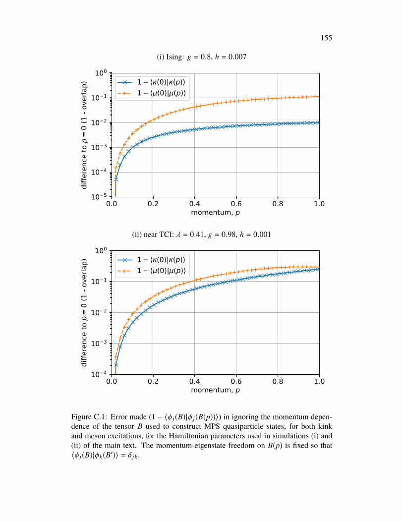
155

(i) Ising: g = 0.8, h = 0.007

0.0 0.2 0.4 0.6 0.8 1.0momentum, p

10 5

10 4

10 3

10 2

10 1

100

diffe

renc

e to

p=

0 (1

- ov

erla

p) 1 (0)| (p)1 (0)| (p)

(ii) near TCI: λ = 0.41, g = 0.98, h = 0.001

0.0 0.2 0.4 0.6 0.8 1.0momentum, p

10 4

10 3

10 2

10 1

100

diffe

renc

e to

p=

0 (1

- ov

erla

p) 1 (0)| (p)1 (0)| (p)

Figure C.1: Error made (1 − 〈φ j(B)|φ j(B(p))〉) in ignoring the momentum depen-dence of the tensor B used to construct MPS quasiparticle states, for both kinkand meson excitations, for the Hamiltonian parameters used in simulations (i) and(ii) of the main text. The momentum-eigenstate freedom on B(p) is fixed so that〈φ j(B)|φk(B′)〉 = δ j k .

156

excitations and we cannot find them by solving the effective Hamiltonian for theB tensors considered above. Nevertheless, we expect there to be excitations thatbehave as quasiparticles subject to a confining force (which makes them accelerate).If one could somehow negate the confining force, as if by accelerating at the samerate as the quasiparticle, the latter would appear to propagate freely.

With this picture in mind, we define a modified energy function

E =∑

j k

eip(k− j)〈φ j |(H − ∆E j 1)|φk〉, (C.18)

where ∆E j :=∑ j−∞ eL +

∑∞j+1 eR and eL , eR are the energy densities of the vacua

parameterized by AL and AR, respectively. Here, it is assumed that the momentum-eigenstate gauge-freedom on B, (C.13), has been fixed so that 〈φ j |φk〉 = δ j k .With orthogonality of the position states, the identity term simply shifts the energyof the excitation in a position-dependent way, cancelling the position-dependentcontribution due to the differing bulk energy densities. One can also write down amodified Hamiltonian

H = H −∑

j

Pj∆E j, (C.19)

where Pj is a projector onto the space of states spanned by |φ j(B)〉 for all B

satisfying the chosen orthogonality conditions: for such B, we thus have Pj |φk(B)〉 =

δ j k |φk(B)〉. We can then rewrite E as

E = 〈φ(AL, B, AR, p)|H |φ(AL, B, AR, p)〉. (C.20)

We can thus optimize B by computing eigenvalue-eigenvector pairs of H, afterpushing it into the ansatz space, analogously to the symmetric case above.

In this formulation it is manifest that the optimization procedure depends on theconditions used to achieve position-state orthogonality, since different conditionswill lead to different Pj in (C.19). In practice, we find that the difference this makesto the resulting optimized states |φ(AL, B, AR, p)〉 is small: We consider the infidelityper site

1 − |Z|−1 |〈φ(BLF, p)|φ(BRF, p)〉| =

1 − |〈φ j(BLF)|φ(BRF, p)〉

, (C.21)

where BLF and BRF are optimized for the same quasiparticle (and momentum p)using the left and right orthogonality conditions, (C.14) and (C.16), respectively,

157

and |Z| is the cardinality of the integers (accounting for the infinite norm of themomentum eigenstates). We find empirically the infidelity scales as h2, whereh 1 is the symmetry-breaking parameter of the Hamiltonian, for the lowest-energy kink states and the Hamiltonian parameters considered in this paper. Thisdependence is shown in Fig. C.2.

It may be possible to design improved optimization techniques that avoid this ambi-guity. A prerequisite would be a cost function other than 〈H〉, presumably relatedto the stability of the quasiparticle wavepackets, that distinguishes usefully betweenthe different choices that can be made in parameterizing B.

Another important observation is that, in (C.19), we assume that the location j ofthe B tensor reliably indicates the position of the kink (or antikink). In fact, sincethe excitation described by B is quasilocal, the location of the kink (defined as thepoint in space at which the spin expectation value crosses zero) may differ from j.Indeed, as shown below in Fig. C.3, there may be a relative shift of several latticesites, depending on the choice of left or right orthogonality conditions on B. Theshift will generally also depend on the momentum p, such that a dispersion relationE(p) computed from the eigenvalues of H should really be interpreted as a functionof the B-tensor momentum, derived from the position j of B, considered distinctfrom the kink momentum, derived from the kink position.

Themomentum-dependent energy-shift due to these position shifts can be calculatedby first computing the actual kink positions, relative to j, for each |φ j(p)〉, as afunction of p. These shifts can then be multiplied by the false-vacuum excessenergy density to compute the energy shift, which can in turn be used to "correct” thedispersion relation. This provides a more intuitive definition of the kink dispersionin the symmetry-broken setting. Note also, however, that since kink quasiparticlesdo not have a well-defined energy gap with respect to the vacuum state, thesedispersion relations still cannot be used to compute particle-production thresholds.They could, however, be used to estimate the kink velocity dE(p)/dp, this beingindependent of energy shifts E(p) → E(p) + c.

WavepacketsAnalogously to the momentum eigenstates of (C.12), we can construct wavepacketsfrom the localized quasiparticle states as

|φ(AL, B, AR, f )〉 :=∑

i

fi |φi(AL, B, AR)〉, (C.22)

158

10 5 10 4 10 3

long. field, h

10 8

10 7

10 6

10 5ba

sis c

hoice

erro

r (pr

obab

ility) near TCI: = 0.41, g = 0.98

Ising: g = 0.8Ising: g = 0.95

Figure C.2: Estimated error (1 - infidelity per site) on momentum eigenstates|φ(B, p)〉 for kink quasiparticles, due to the choice of orthogonality conditionson B used to achieve 〈φ j(B)|φk(B)〉 = δ j k . Here we compare the left and rightorthogonality conditions, (C.14) and (C.16).

where in our simulations we choose fi to be a Gaussian centered at position x

with width σ. Importantly for our purposes, it is straightforward to turn such awavepacket state into a single MPS:

|φ(AL, B, AR, f )〉 =∑®s

w†L

(∞∏

i=−∞

Asii

)wR |®s〉, (C.23)

where

Asi :=

(As

L fi Bs

0 AsR

)(C.24)

is a 2D × 2D matrix, given that AsL , As

R, and Bs are all D × D matrices. We set theboundary conditions to be

w†L :=(v†L, 0

)wR :=

(0vR

)(C.25)

for some generic choice of vL and vR. If | fi | falls below some numerical threshold forall i less than some iL and for all i greater than some iR > iL , we can truncate it to zeroand reduce the bond dimension to D in those regions without introducing significant

159

errors. This allows us to represent a truncated wavepacket in the thermodynamiclimit using the nonuniform window ansatz (C.3).

As discussed in the main text, this wavepacket construction ignores any momentumdependence of the tensor B. While this introduces errors in the form of contributionsfrom other excitations, as shown in Fig. C.3, these become small for large σ, asindicated in Fig. C.5 below.

Localized states and Bloch-state parameter redundancyThe parameter redundancy, or "gauge freedom”, on the B-tensors of the momentumeigenstates (C.12) does not leave the localized states |φ j(B)〉 of (C.11) unchanged.These states, as well as the wavepacket states (C.22) built from them, depend on howthese degrees of freedom are fixed. However, the procedure we use for choosingoptimal B tensors is based on momentum eigenstates and does not tell us how tooptimally fix the remaining freedom.

That said, the impact of this choice on Gaussian wavepacket states must vanish inthe limit σ → ∞, where packets become momentum eigenstates. Hence we canreasonably expect the impact on wavepackets with finite width to become small asσ increases. Since we already have a physical reason to choose broad wavepacketsin our simulations (for slow wavepacket spread), this issue is not as severe as it mayat first appear.

Nevertheless, we choose to use the reflection-symmetric conditions of [239], slightlyadapted for the topologically nontrivial setting, to fix the remaining freedom on theB tensors used to construct our initial bubble states. To be precise, we fix B bychoosing x in (C.13) as

x = arg minx′

©­«∑

s

B(x′)(s) ⊗ A(s)L∗

2 +∑s

B(x′)(s) ⊗ A(s)R∗

2ª®¬ . (C.26)

In terms of tensor networks, we can rewrite this as

x = arg minx′

©­« 𝐴𝐿

𝐵(𝑥′)

*

2 + 𝐵(𝑥′)

𝐴𝑅*

2ª®¬ . (C.27)

Unlike the left and right orthogonality conditions, (C.14) and (C.16), these condi-tions are manifestly symmetric under spatial reflections. The reflection-symmetric

160

conditions can be formulated as an overdetermined linear-least-squares optimizationproblem and then solved using standard techniques.

See Fig. C.3 for a comparison of the reflection-symmetric conditions to the left andright orthogonality conditions, in terms of the spin expectation values of localizedtopological states. We plot these results for AL and AR representing the two vacuaof the Ising chain (λ = 0, g = 0.8) for both zero and nonzero longitudinal fieldstrength h. The tensor B is variationally optimized, as described above, so that themomentum eigenstate |φ(AL, B, AR, p = 0)〉 approximates the lowest-lying topolog-ical excitation. We note that, although the symmetrized states exhibit "smoother”spin expectation values in both cases, they are not perfectly symmetric in the caseh > 0. The spatial asymmetry in the spin likely reflects the energetic asymme-try of topological states in this case. In both cases, there is certainly an aestheticimprovement to be had by imposing the symmetrization conditions, but it remainsto be seen whether the symmetrized states are better representations of localizedquasiparticles. To see that they are, we consider how well wavepackets built fromthem fit into the corresponding quasiparticle subspace.

In Fig. C.5, we plot the portion of a kink wavepacket state (by probability) outsideof the targeted kink-quasiparticle subspace for both the orthogonal and reflection-symmetric conditions. We explain how to carry out this kind of projection inApp. C.4. We observe that the symmetrized states result in a much more accuratewavepacket than the orthonormal states, by almost two orders of magnitude, con-firming that the symmetrized choices are more than just aesthetically pleasing. Inthe symmetric Ising model (h = 0), we can also compare the energy of wavepackets.In Fig. C.4, we see that the kink wavepackets created with the symmetrized stateshave consistently lower energy, which indicates improved accuracy, since we aretargeting the lowest-lying kink quasiparticle.

Two-particle statesTo create false-vacuum bubbles, we need to combine two quasiparticles, namely akink and an antikink. Two-particle states have the form

|φφ j k(AL, BL, AC, BR, AR)〉 :=∑®s

|®s〉×

v†L

( j−1∏i=−∞

AsiL

)Bsj

L

(k−1∏

l=i+1Asl

C

)Bsk

R

(∞∏

m=l+1Asm

R

)vR, (C.28)

161

(i) Ising: g = 0.8, h = 0.007

0 20 40 60 80 100position

0.75

0.50

0.25

0.00

0.25

0.50

0.75

Zleft orthogonalright orthogonalsymmetrized (left)symmetrized (right)

(ii)near TCI: λ = 0.41, g = 0.98, h = 0.001

0 20 40 60 80 100position

1.0

0.5

0.0

0.5

1.0

Z

left orthogonalright orthogonalsymmetrized (left)symmetrized (right)

Figure C.3: Spin expectation values of a kink position MPS |κ j〉 for (i) the Isingmodel and (ii) close to the Tri-Critical-Ising (TCI) point. The bond dimensionis D = 8 for the Ising data, and D = 18 for the TCI data. We plot the spinsfor various ways of fixing the momentum-eigenstate freedom: the left and rightorthogonal conditions, (C.14) or (C.16), and the reflection-symmetric conditions(C.26), beginning from a B tensor optimized using either the left or right conditions(since this makes a small physical difference to the result – see App. C.3).

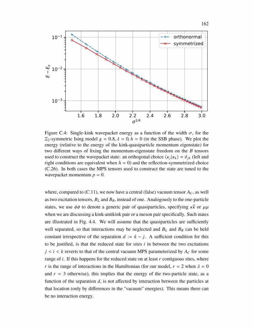
162

1.6 1.8 2.0 2.2 2.4 2.6 2.8 3.01/4

10 3

10 2

10 1

EE

orthonormalsymmetrized

Figure C.4: Single-kink wavepacket energy as a function of the width σ, for theZ2-symmetric Ising model g = 0.8, λ = 0, h = 0 (in the SSB phase). We plot theenergy (relative to the energy of the kink-quasiparticle momentum eigenstate) fortwo different ways of fixing the momentum-eigenstate freedom on the B tensorsused to construct the wavepacket state: an orthogonal choice 〈κ j |κk〉 = δ j k (left andright conditions are equivalent when h = 0) and the reflection-symmetrized choice(C.26). In both cases the MPS tensors used to construct the state are tuned to thewavepacket momentum p = 0.

where, compared to (C.11), we now have a central (false) vacuum tensor AC , as wellas two excitation tensors, BL and BR, instead of one. Analogously to the one-particlestates, we use φφ to denote a generic pair of quasiparticles, specifying κκ or µµwhen we are discussing a kink-antikink pair or a meson pair specifically. Such statesare illustrated in Fig. 4.4. We will assume that the quasiparticles are sufficientlywell separated, so that interactions may be neglected and BL and BR can be heldconstant irrespective of the separation d := k − j. A sufficient condition for thisto be justified, is that the reduced state for sites i in between the two excitationsj < i < k reverts to that of the central vacuum MPS parameterized by AC for somerange of i. If this happens for the reduced state on at least r contiguous sites, wherer is the range of interactions in the Hamiltonian (for our model, r = 2 when λ = 0and r = 3 otherwise), this implies that the energy of the two-particle state, as afunction of the separation d, is not affected by interaction between the particles atthat location (only by differences in the "vacuum” energies). This means there canbe no interaction energy.

163

1.6 1.8 2.0 2.2 2.4 2.6 2.8 3.01/4

10 7

10 6

10 5

10 4

10 3

P( n

ot in

(0

) sub

spac

e )

left orthogonalsymmetrized (left)

Figure C.5: Portion of a single-kink wavepacket state outside of the single-kinksubspace κ(0) as a function of the wavepacket width σ, for the Z2-broken Isingmodel g = 0.8, λ = 0, h = 0.007. We plot the error for two different waysof fixing the momentum-eigenstate freedom on the B tensors used to construct thewavepacket: the left orthogonal choice 〈κ j |κk〉 = δ j k and the reflection-symmetrizedchoice (with B optimized using the left orthogonal conditions). In both cases theMPS tensors used to construct the state are tuned to the wavepacket momentum,which is p = 0. The projection into the κ(0) subspace uses B tensors optimized usingthe left orthogonal conditions and fully accounts for momentum dependence via aFourier analysis.

This condition can be made more precise: we define the strength of interactioneffects at location i (with j < i < k) as the deviation of the left and right environmenttensors of the 2-particle state from the corresponding environment tensors of thecentral (false) vacuum MPS parameterized by AC . Here, the environment at site i

is the tensor network for the reduced state on site i, excluding the tensors assignedto site i itself. It naturally splits into left and right components, consisting of thetensors to the left and to the right of i, respectively. We compute the deviationfor the left and right parts separately, as the norm of the difference between thecentral (false) vacuum environment and the 2-particle-state environments. For theleft environment, we define

εL(i) :=

𝐴𝐶

𝐴𝐶

*𝐴𝐶

𝐴𝐶

*𝐵𝐿

𝑙𝐿 *

𝐵𝐿. . . − 𝑙𝐶

, (C.29)

where the ellipsis indicates that the center transfer matrix should be repeated as

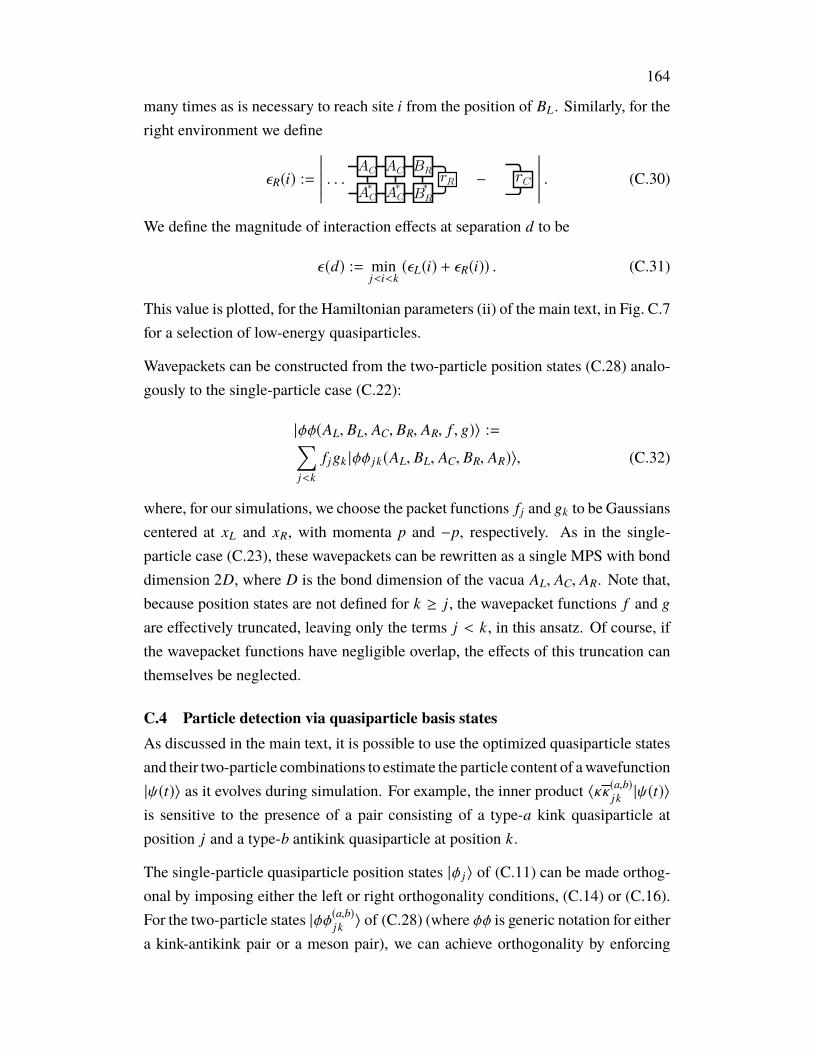
164

many times as is necessary to reach site i from the position of BL . Similarly, for theright environment we define

εR(i) :=

. . . 𝐵𝑅

𝐵𝑅𝑟𝑅

*𝐴𝐶

𝐴𝐶

*𝐴𝐶

𝐴𝐶

*− 𝑟𝐶

. (C.30)

We define the magnitude of interaction effects at separation d to be

ε(d) := minj<i<k(εL(i) + εR(i)) . (C.31)

This value is plotted, for the Hamiltonian parameters (ii) of the main text, in Fig. C.7for a selection of low-energy quasiparticles.

Wavepackets can be constructed from the two-particle position states (C.28) analo-gously to the single-particle case (C.22):

|φφ(AL, BL, AC, BR, AR, f , g)〉 :=∑j<k

f jgk |φφ j k(AL, BL, AC, BR, AR)〉, (C.32)

where, for our simulations, we choose the packet functions f j and gk to be Gaussianscentered at xL and xR, with momenta p and −p, respectively. As in the single-particle case (C.23), these wavepackets can be rewritten as a single MPS with bonddimension 2D, where D is the bond dimension of the vacua AL, AC, AR. Note that,because position states are not defined for k ≥ j, the wavepacket functions f and g

are effectively truncated, leaving only the terms j < k, in this ansatz. Of course, ifthe wavepacket functions have negligible overlap, the effects of this truncation canthemselves be neglected.

C.4 Particle detection via quasiparticle basis statesAs discussed in the main text, it is possible to use the optimized quasiparticle statesand their two-particle combinations to estimate the particle content of awavefunction|ψ(t)〉 as it evolves during simulation. For example, the inner product 〈κκ(a,b)j k |ψ(t)〉

is sensitive to the presence of a pair consisting of a type-a kink quasiparticle atposition j and a type-b antikink quasiparticle at position k.

The single-particle quasiparticle position states |φ j〉 of (C.11) can be made orthog-onal by imposing either the left or right orthogonality conditions, (C.14) or (C.16).For the two-particle states |φφ(a,b)j k 〉 of (C.28) (where φφ is generic notation for eithera kink-antikink pair or a meson pair), we can achieve orthogonality by enforcing

165

the left orthogonality conditions on the left excitation tensor, BL , and the right or-thogonality conditions on right excitation tensor, BR. With these conditions, thetwo-particle states are orthogonal for one pair of species a, b

〈φφ(a,b)j k |φφ

(a,b)lm 〉 = δ jlδkm. (C.33)

Furthermore, by limiting the subspace to states with separation d := k − j largeenough so that interaction effects are negligible (see App. C.3), we can achieve anapproximately orthonormal basis across species as well as positions:

〈φφ(a,b)j k |φφ

(c,d)lm 〉 ≈ δ jlδkmδacδbd ∀ k j, m l . (C.34)

If the left and right bulk vacuum tensors, AL and AR of the evolved state |ψ(t)〉, whichin our simulations have the form (C.3), match the left and right bulk tensors AL andAR in the two-particle states (C.28), it is then straightforward to (approximately)project |ψ(t)〉 into the subspace spanned by these states.

However, we must take care when interpreting the overlaps of a wavefunction|ψ(t)〉 with quasiparticle position states such as |φ j(B)〉, as should be clear fromthe discussion of excitation tensors and quasiparticle position states above. Inparticular, the momentum-dependence of the B tensors optimized to represent eachquasiparticle, as well as the ambiguity in fixing the degrees of freedom (C.13)in B that are not fixed by the optimization procedure (see App. C.3), make theinterpretation of the overlap unclear unless the quasiparticle content of |ψ(t)〉 consistsof broad spatial wavepackets, whose momentum support is focused around themomentum p used to optimize the B tensor. We next discuss two methods foravoiding these issues.

Checking consistency in the projected wavefunctionAs described in the main text, one way to avoid issues with momentum-dependenceand wavepacket breadth is to choose some momentum p, optimize a tensor B(p)

at that momentum for the quasiparticle being targeted, then examine the overlapsψ j := 〈φ j(B(p))|ψ(t)〉 (or ψ j k := 〈φφ j k(B(p), B′(p′))|ψ(t)〉 for a two-particle basis).If the wavepacket width of the projected wavefunction ψ j is sufficiently large, andthe momentum support (computed via Fourier transformation) sufficiently close tothe chosen value of p, we know that the error made is small and can trust that theprojection is accurately telling us about the quasiparticle content. We can quantifyhow broad the wavepacket must be, and how close the wavepacket momenta shouldbe to p, via analyses such as those of Fig. C.3 and Fig. C.5.

166

If the distribution of momenta in the wavepacket indicates a large error due to thechoice of p made while constructing the basis, it may be possible to iteratively tunep to achieve a better match. This procedure fails, of course, if the wavepackets in|ψ(t)〉 are too narrow in position space (and hence too broad in momentum space)for the error to be kept small.

We use this procedure to compute the spin expectations values within each particle"sector” in Fig. 4.8, tuning the basis momenta pL and pR for two-particle bases|φφ j k(BL(pL), BR(pR)〉 to match the observed momenta.

Fourier analysisTo fully account for the momentum-dependence of the quasiparticle states, and toeliminate any issues due to the momentum-eigenstate "gauge-freedom” (C.13) on B

tensors, we can simply take overlaps with momentum eigenstates instead of with theposition states. These states are exactly invariant under (C.13), and the B tensorsused to construct them can be optimized for the momentum of the eigenstate to avoidmomentum mismatch.

For example, to project onto a single-particle subspace at momentum p, one cancompute 〈φ(p)|ψ(t)〉, with |φ(p)〉 from (C.12). We can expand this overlap in termsof position states:

〈φ(B(p), p)|ψ(t)〉 =∑

j

e−ipj 〈φ j(B(p))|ψ(t)〉, (C.35)

where B(p) is an excitation tensor optimized to represent the quasiparticle φ atmomentum p. This overlap can be computed in practice, despite the infinite sumover j, because the position of excitations in |ψ(t)〉 is limited to the nonuniformwindow of (C.3) in which the initial quasiparticles (comprising the bubble) wereplaced, so that there are only ∼ N nonzero position terms in this overlap.

To compute the projection onto the entire quasiparticle subspace, we must evaluatethe integral ∫ π

−πdp 〈φ(p)|ψ(t)〉. (C.36)

This can be done approximately by sampling, for example using a numerical inte-gration scheme. In practice, we use the Fast Fourier-Transform (FFT) algorithm totransform the spatial components 〈φ j(B(p))|ψ(t)〉 into a fixed sampling of momen-tum components at a resolution determined by the number of lattice sites N summedover in (C.35).

167

We use this method to compute the projected single-kink wavefunction described inFig. C.5, to compute the kink-antikink scattering outcome probability in Fig. 4.6 ofthe main text, and to compute the various scattering outcome probabilities reportedin Fig. 4.8.

Efficient computation of the quasiparticle Fourier analysis

The projection of a wavefunction |ψ(t)〉 onto many momentum modes is relativelycomputationally intensive, since for each momentum mode we must first com-pute a tuned excitation tensor B(p), followed by a full set of position overlaps〈φ j(B(p))|ψ(t)〉. In the case of single-particle states, the cost is O(N M), where M isthe number of momentum samples and N is the nonuniform window size of |ψ(t)〉.For two-particle states, since we must consider cases in which the two particles havedifferent momenta/positions, making the cost O(M2N2). If M ∼ N , and N ≈ 1000,this may be prohibitive!

To reduce the cost, we can use the observation that the optimized excitation tensorB(p), for a given quasiparticle, usually varies only slowly with the quasiparticlemomentum p by introducing a small momentum mismatch in a controlled way: Weproject the excitation tensors B(p), optimized for each mode of momentum p that wewish to sum over, onto a small basis of excitation tensors that capture the momentumdependence accurately across a wide range of p:

B(p) ≈∑α

bα(p)Bα, (C.37)

for appropriately chosen coefficients bα(p) and suitably chosen basis tensors Bα.A suitable basis can be built by orthonormalizing (via a Gram-Schmidt procedure)a set of B(pα) obtained at a selection of momenta (say, p = −2,−1, 0, 1, 2). Wefind that < 10 basis tensors is sufficient, for our chosen Hamiltonian parameters,to achieve an accuracy of ∼ 10−8 in (C.37). Given such a basis, we then computeposition-state overlaps only for the basis tensors, from which we can compute theprojection of the wavefunction onto an arbitrary momentum mode while makingonly a small error.

For example, in the case of a two-particle basis, we first compute ψ j k;αβ :=〈φφ j k(BL,α, BR,β)|ψ(t)〉. Then, using the coefficients of (C.37), we approximatethe overlap with the momentum-tuned position states as

〈φφ j k(BL(p), BR(p′))|ψ(t)〉 ≈ b∗L,α(p)b∗R,β(p

′)ψ j k;αβ. (C.38)

From here, the momentum-mode overlaps are but an FFT away.

168

Other sources of errorEven for the Fourier analysis, there are at least two sources of inaccuracy beyondthe choice of iMPS bond dimensions in the vacua and the quality of the optimiza-tion procedures used to find the vacua and the excitations tensors B. First, thereis the further ambiguity (see App. C.3) in the case of topological excitations in thesymmetry-broken setting (h > 0) owing to the dependence of the B-tensor optimiza-tion on an arbitrary choice of orthogonality conditions made during optimization.We do not currently know of a way to avoid this source of error. Fortunately, asillustrated in Fig C.2, we have good evidence that it is small.

The other source of error comes from interaction effects, which are not capturedproperly by the two-particle states. As discussed above, one can choose the mini-mum separation of the two particles to avoid interaction, by throwing out positionstates where the "interaction strength” ε , defined in (C.31), rises above some thresh-old. In choosing the threshold, there is a tradeoff between capturing (potentiallylarge) components of the wavefunction that have smaller separation, but likely incursome (possibly small) error due to interaction, and the magnitude of ε , which isa conservative estimate of that error and is exponential in the separation. How tomake this tradeoff optimally depends on the target wavefunction and the requiredprecision of the projected wavefunction.

For our computations, we examined the dependence of the norm of the projectedwavefunctions on the minimum separation dmin allowed in the two-particle basisstates. Exemplary results are shown in Figs. C.6 and C.7, which also show thedependence of the norms on the simulation bond-dimension limit. In Fig. C.6, weobserve that, for the largest bond-dimension, the norm of the projected wavefunctionis essentially constant for d < 70, despite the rising magnitude of interaction effects.This suggests that the wavefunction has negligible support at small separations(which we confirm via a Fourier analysis). We also observe that a minimumseparation of dmin = 60 is sufficient to keep ε < 10−6. Noting that the interactionstrength is a property of the quasiparticle basis, and hence independent of time, wemake the choice dmin = 60 to avoid interaction effects when computing the datashown in Fig. 4.6 of the main text.

Fig. C.7 shows similar data for three quasiparticle-pair "sectors” for the Hamiltonianparameters (ii) of the main text. This data was used to estimate the scatteringoutcome probabilities shown in Fig. 4.8 of the main text. We see that, for this targetwavefunction |ψ(t)〉, interaction effects are not important for the κκ(0,0) and µµ(0,0)

169

0 20 40 60 80 100 120min. two-particle separation, dmin

10 4

10 3

10 2

10 1

P( n

ot in

(0

,0) s

ubsp

ace

)

10 10

10 8

10 6

10 4

10 2

inte

ract

ion

effe

cts

D 32D 64D 128interaction effects

Figure C.6: Portion of the evolved bubble wavefunction outside of the kink-antikink"sector” for simulation (i) of Fig. 4.5 (λ = 0, g = 0.8, h = 0.007) at time t = 150,as a function of the minimum separation dmin := min(k − j) permitted in the two-quasiparticles basis states |κκ(0,0)j,k 〉. Probabilities are computed via a Fourier analysis,taking into account the momentum-dependence of the basis states. The basis errordue to interaction effects is estimated using (C.31).

"sectors”. However, they may influence the result at the level of ∼ 0.01, possiblymore, for κκ(0,1) (and, by reflection symmetry of the initial bubble state, κκ(1,0)). Theκκ(0,1) and κκ(1,0) results are likely to be more sensitive to interaction than the κκ(0,0)

result because the former two "sectors” describe bubble states in which one of thewalls (the kink or the antikink) is heavier than in the κκ(0,0) case. These "lopsided”bubbles will be smaller than a κκ(0,0) bubble at the same energy, leading to largercomponents of the wavefunction at small separations, where interaction effects arestronger.

C.5 Evolving through timeTo evolve an initial bubble iMPS in time, we define a window of N lattice sitessurrounding the bubble and allow the MPS tensors belonging to those sites to varyduring the evolution, while keeping the rest of the MPS tensors fixed. In otherwords, we use the nonuniform window ansatz (C.3) with fixed bulk tensors AL ,AR. To compute the evolved state, we use methods based on the Time-DependentVariational Principle (TDVP), which is set out for this class of states in [261] andimplemented in the evoMPS package [264].

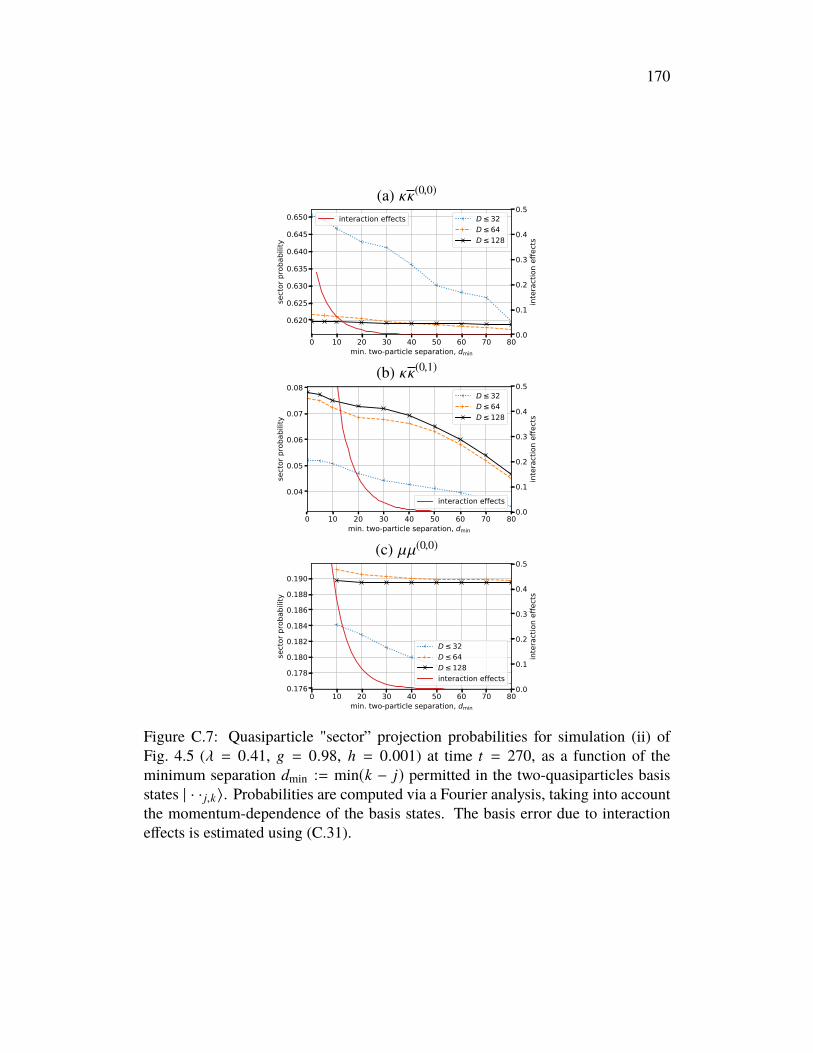
170

(a) κκ(0,0)

0 10 20 30 40 50 60 70 80min. two-particle separation, dmin

0.620

0.625

0.630

0.635

0.640

0.645

0.650

sect

or p

roba

bilit

y

D 32D 64D 128

0.0

0.1

0.2

0.3

0.4

0.5

inte

ract

ion

effe

cts

interaction effects

(b) κκ(0,1)

0 10 20 30 40 50 60 70 80min. two-particle separation, dmin

0.04

0.05

0.06

0.07

0.08

sect

or p

roba

bilit

y

D 32D 64D 128

0.0

0.1

0.2

0.3

0.4

0.5

inte

ract

ion

effe

cts

interaction effects

(c) µµ(0,0)

0 10 20 30 40 50 60 70 80min. two-particle separation, dmin

0.176

0.178

0.180

0.182

0.184

0.186

0.188

0.190

sect

or p

roba

bilit

y

0.0

0.1

0.2

0.3

0.4

0.5

inte

ract

ion

effe

cts

D 32D 64D 128interaction effects

Figure C.7: Quasiparticle "sector” projection probabilities for simulation (ii) ofFig. 4.5 (λ = 0.41, g = 0.98, h = 0.001) at time t = 270, as a function of theminimum separation dmin := min(k − j) permitted in the two-quasiparticles basisstates | · · j,k〉. Probabilities are computed via a Fourier analysis, taking into accountthe momentum-dependence of the basis states. The basis error due to interactioneffects is estimated using (C.31).

171

The TDVP provides flow equations that describe the evolution of the MPS tensorsneeded to optimally approximate the evolution of the state by the Hamiltonian, giventhe constraint that the MPS bond dimension must remain fixed. Various schemescan be used to integrate the flow equations: we use the popular Runge-Kutta 4/5(RK4) numerical integrator (to directly integrate the global flow equations) as wellas the "projector-splitting” (PS) integrator of [263]. Since we want the MPS bonddimension to grow as needed (up to some maximum) as the entanglement of thestate increases, we combine TDVP flow with techniques for increasing the bonddimension. In particular, we use the "dynamical expansion” scheme described in[258] together with the RK4 integrator, as well as the two-site projector-splittingmethod of [263].

The PS method and the RK4 integrator (with dynamical expansion), despite hav-ing similar theoretical error rates for a given time-step size, behave differently inimportant ways. For a given step size, the PS method has a larger computationaloverhead per step, but has better numerical stability and precision since, unlike the"traditional” TDVP scheme of [258], it does not require the inversion of matriceswith small eigenvalues.

We find that the RK4 scheme with dynamical expansion is too unstable to usereliably during the initial timesteps of our simulations, which begin with an MPSof relatively small bond dimension (at most twice the vacuum bond dimension).However, we find RK4 can be used successfully after performing a small number ofinitial steps using the two-site PS scheme. During these initial PS steps, the bonddimension increases significantly. Later in the evolution, once the bond dimensionhas stabilized, we find the much faster RK4 scheme is able to take over withoutsignificant impact on the results. During the evolution, we do allow the MPS bonddimension to grow beyond a predefined maximum value.

To better understand the effects of the integration scheme on our simulations, as wellas the impact of the bond-dimension limit, we compute two quantities indicativeof numerical error: the energy drift and the truncation error. Although the exactevolution of the quantum state conserves the energy, the imperfect integration of theTDVP flow equations, combined with the limited bond dimension, leads to a smallenergy drift. This drift is an indicator of error incurred more generally during theevolution. We estimate the truncation error – the portion of the state by norm that islost due to the bond dimension limit – as the maximum value, taken over position,of the minimum Schmidt coefficient (the Dth-largest) for the left-right bipartition at

172

that position. Since there are rarely large jumps in the Schmidt spectrum, this valueprovides a good estimate of the magnitude of the terms that cannot be representeddue to the bond-dimension limit.

As shown for simulation (ii) of the main text in Fig. C.8, the energy drift is par-ticularly sensitive to the integration scheme and step size, whereas the truncationerror is, unsurprisingly, most sensitive to the bond-dimension limit. We note thatthe truncation error jumps at the time of the first kink-antikink collision (t ≈ 175),consistent with the entanglement jump observed in Fig. 4.9 of the main text. Fig. C.9provides a more detailed picture of the entanglement structure, showing the full en-tanglement (Schmidt) spectrum (up to truncation) before and after the first collisionat the cut with the largest entanglement entropy.

The computational cost of simulating up to some fixed time t scales as O(

D3

δt

).

We are therefore eventually forced to trade accuracy for computational cost. Forthis particular simulation, we judge D ≤ 128 and δt = 0.05 to provide sufficientaccuracy, while keeping the computational requirements manageable, to enable usto study the outcomes of at least the first kink-antikink collision event in detail.

C.6 Comparison with quench approachesWe construct our initial false-vacuum bubble from individual kink and antikinkquasiparticles, separated by a region of metastable false vacuum. Similar states canbe constructed via a simpler approach: act on the uniform true vacuum |Ω〉 with asuitable string operator that, in the case of the Ising-type model we study, flips allthe spins over a range of sites:

|Sj k〉 := X j X j+1 . . . Xk−1Xk |Ω〉 (C.39)

For small longitudinal field h, we know that flipping all the spins gets us from thevacuum to a state close to the false vacuum (see App. C.2), so if d := k − j issufficiently large, the reduced state will be close to that of the false vacuum in themiddle of the flipped region and topological excitations will be created at the edgesof the string. In general, these excitations will be a combination of many topologicalquasiparticles of varying energy, hence the walls of a bubble created in this way willbe unstable to interactions between these quasiparticles. The walls are also highlylocalized in position and hence have large momentum uncertainty.

By smearing the edges of the string in space, their momenta can be focused. This

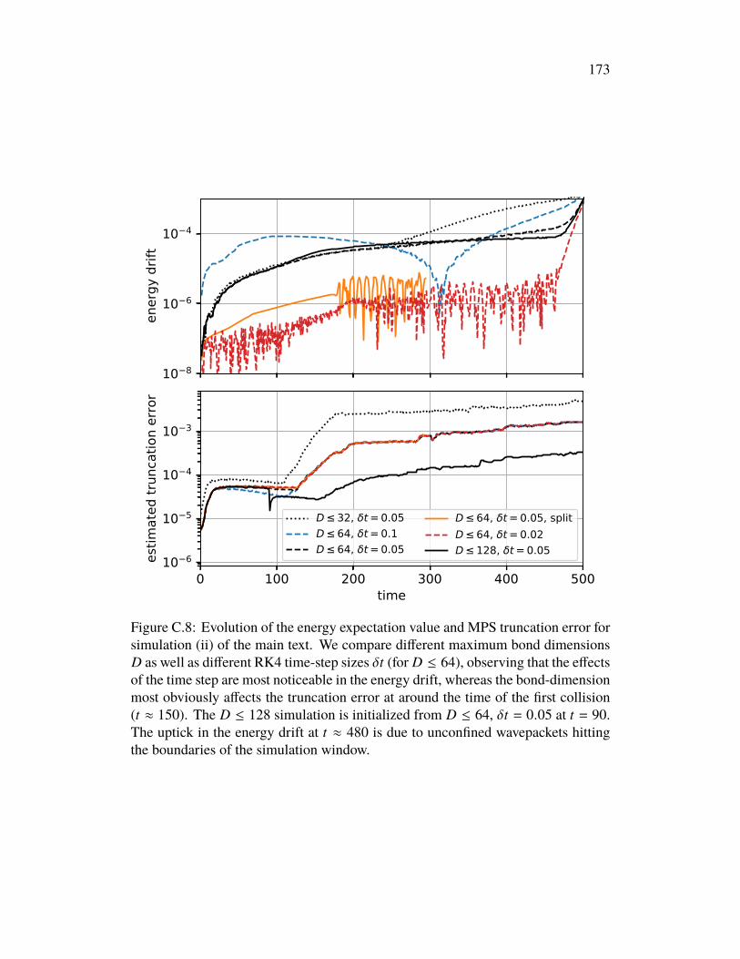
173

10 8

10 6

10 4

ener

gy d

rift

0 100 200 300 400 500time

10 6

10 5

10 4

10 3

estim

ated

trun

catio

n er

ror

D 32, t = 0.05D 64, t = 0.1D 64, t = 0.05

D 64, t = 0.05, splitD 64, t = 0.02D 128, t = 0.05

Figure C.8: Evolution of the energy expectation value and MPS truncation error forsimulation (ii) of the main text. We compare different maximum bond dimensionsD as well as different RK4 time-step sizes δt (for D ≤ 64), observing that the effectsof the time step are most noticeable in the energy drift, whereas the bond-dimensionmost obviously affects the truncation error at around the time of the first collision(t ≈ 150). The D ≤ 128 simulation is initialized from D ≤ 64, δt = 0.05 at t = 90.The uptick in the energy drift at t ≈ 480 is due to unconfined wavepackets hittingthe boundaries of the simulation window.

174

0 20 40 60 80 100 120Schmidt coefficient number (size order)

10 5

10 4

10 3

10 2

10 1

100

Max

-cut

Sch

mid

t spe

ctru

m

before collision (t = 100)after collision (t = 300)

Figure C.9: Schmidt spectra for the maximum-entropy cut before and after the firstcollision in simulation (ii) of the main text. The bond dimension is 128.

results in states of the form

|Ψ〉 =∑j<k

f j(xL, pL) fk(xR, pR)|Sj k〉, (C.40)

where f j and fk are wavepacket functions for the left and right edge, respectively.If we choose these to be Gaussian, as for the wavepackets in the main text, we geta bubble state similar to those used in the main text, except that the walls haveundetermined quasiparticle content.

In Fig. C.10, we compare the dynamics of three different initial states for theHamiltonian parameters (ii) of the main text: (a) the fully localized string of (C.39),(b) the smeared string of (C.40), and (c) the tuned quasiparticle kink-antikinkwavepackets used in the main text. We choose the same kink-antikink separation inall cases, and the same wavepacket widths in the latter two. The TDVP step size andthe maximum bond dimension were also the same in all three cases. Simulations(a) and (b) both exhibit clear ballistic spread of energy from the initial bubbleedges, indicating their instability, whereas simulation (c) only shows ballistic spreadafter the initial bubble walls have collided, consistent with the walls consisting ofindividual quasiparticles.

It is noteworthy that the evolution of state (a) encounters catastrophic numericalerrors at around t = 150, unlike simulations (b) and (c), suggesting that scenario

175

(a) is much harder to simulate accurately4. In Fig. C.11 we show the energy driftand estimated truncation error (smallest retained Schmidt coefficient for the mostentangled cut) for the same three simulations. This data clearly indicates thatsimulation (c) is easiest to simulate, since both the energy drift and the truncationerror remain smaller with the same evolution parameters. The large truncation errorat early times in cases (a) and (b) is consistent with a large amount of entanglementbeing generated early on, coming from the multiple excitations created at the endsof the string operator.

C.7 Velocity and Bloch oscillationsSingle-kink evolutionIn case of explicit symmetry breaking (h > 0), an isolated kink wavepacket, withtrue vacuum on one side and false vacuum on the other, will accelerate toward thefalse vacuum, absorbing the excess energy density of the latter. On the lattice,however, the kinetic energy cannot increase indefinitely. Instead, as discussed in themain text, the kink begins to undergo Bloch oscillations, eventually decelerating andreversing its direction of travel, as shown in Fig C.12 for Ising model parameters.By projecting into the κ basis of single kinks (see App. C.4), we can easily computethe kink position and momentum for such a simulation. As shown in Fig. C.13, themomentum increases linearly with time, making it easy to understand the evolutionof the wavepacket position via the group velocity, which is given by dE(p)/dp,where E(p) is the quasiparticle dispersion relation. In Fig. C.14 we show thevelocity derived from the position of Fig. C.13, compared to the velocity derivedfrom the momentum of Fig. C.13, via the dispersion relation.

Bubble evolutionIn the case of a bubble state, the initial kink and antikink behave as their isolatedcounterparts, accelerating into the false vacuum until they near each other andinteract. Their momenta increase linearly until the collision, as shown in latticeunits (−π < p ≤ π) for the Ising model (parameter set (i) of the main text) inFig. C.15. It is interesting to note that the momentum variance is significantly largerafter the collision than it is before, indicative of an (in this case elastic) interaction.

The velocity of the kink and antikink, defined here as the velocity of the point inspace atwhich the (interpolated) spin expectation value crosses zero, evolve as shown

4These errors also occur if the PS integrator is used throughout the evolution, rather thanswitching to RK4 after some entanglement has built up.

176

200

400

time

(a) bare string (b) bare string, smeared

(c) quasiparticle packets

200

400

time

0 500position

200

400

time

0 500position

0 500position

1

0

1

Z

6

4

2

log(

|e/E

|)

0

2

4

cut e

ntro

py

Figure C.10: Evolution of spin and energy density expectation values and the cutentropy for parameter set (ii) of the main text (λ = 0.41, g = 0.98, h = 0.001), withthree different initial states. State (a) is prepared by acting on the vacuum with astring operator

∏xR−1j=xL

X j , which flips the spins to forma bubble-like statewith energyE/mµ = 8.69. State (b) is similar to (a), but with the ends of the string smearedout using Gaussian packets of width σ = 40, reducing the energy to E/mµ = 4.02.State (c) is the initial state discussed in the main text with E/mµ = 2.62, usingquasiparticle wavepackets for the kinks and the false vacuum for the middle region.The evolution parameters are the same in all cases: The maximum bond dimensionis 64 and the RK4 step size is 0.05. In (a), dramatic errors in the simulationoccur at t ≈ 150, indicating the difficulty of simulating these dynamics versus (b)and (c). In both (a) and (b), ballistic energy-spread emanating from the initialkinks indicates that they have complex quasiparticle content, resulting in immediateinelastic scattering. In contrast, the tuned quasiparticle kinks of (c) do not produceappreciable ballistic spread until the bubble walls have collided.

177

10 9

10 6

10 3

100

ener

gy d

rift

(a) bare string(b) bare string, smeared(c) quasiparticle packets

0 100 200 300 400 500time

10 5

10 4

10 3

10 2

10 1

estim

ated

trun

catio

n er

ror

(a) bare string(b) bare string, smeared(c) quasiparticle packets

Figure C.11: Evolution of the energy expectation value andMPS truncation error forthe simulations of Fig. C.10. Energy drift (|1−E(t)/E(0)|) indicates deviation fromunitary evolution and results from restriction to a maximum bond dimension of 64as well as from numerical integration errors (RK4 step size 0.05). Truncation error(estimated as the maximum over cuts of the smallest Schmidt coefficient) resultsfrom the limited bond dimension and increases as entanglement is produced.

in Fig. C.16, in accordance with the dispersion relation of the kink quasiparticleexcitation. In this simulation, the kink achieves its maximumvelocity well before thecollision, and begins to decelerate as part of a Bloch oscillation. The pre-collisionvelocity can be kept from reaching its maximum by reducing the kink-antikinkseparation in the initial bubble state, as we have confirmed with other simulations.

In Fig. C.17, we show the kink and antikink velocity evolution for simulation (ii)of the main text. In this case, we have set the initial kink-antikink separation sothat the velocity does not reach a maximum prior to collision (indicating that Blochoscillations have not yet begun).

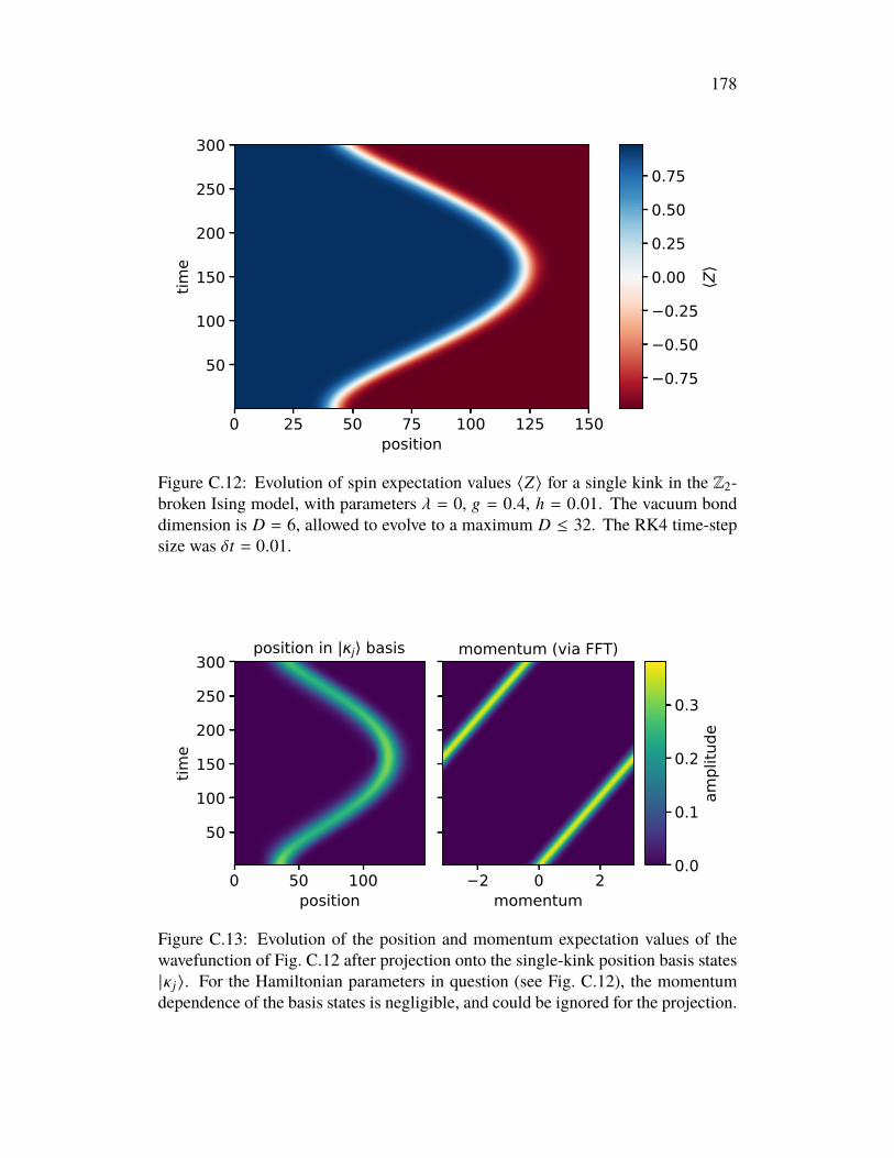
178

0 25 50 75 100 125 150position

50

100

150

200

250

300

time

0.75

0.50

0.25

0.00

0.25

0.50

0.75

Z

Figure C.12: Evolution of spin expectation values 〈Z〉 for a single kink in the Z2-broken Ising model, with parameters λ = 0, g = 0.4, h = 0.01. The vacuum bonddimension is D = 6, allowed to evolve to a maximum D ≤ 32. The RK4 time-stepsize was δt = 0.01.

0 50 100position

50

100

150

200

250

300

time

position in | j basis

2 0 2momentum

momentum (via FFT)

0.0

0.1

0.2

0.3am

plitu

de

Figure C.13: Evolution of the position and momentum expectation values of thewavefunction of Fig. C.12 after projection onto the single-kink position basis states|κ j〉. For the Hamiltonian parameters in question (see Fig. C.12), the momentumdependence of the basis states is negligible, and could be ignored for the projection.

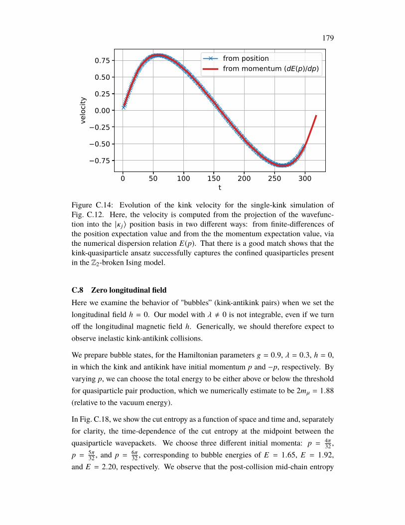
179

0 50 100 150 200 250 300t

0.75

0.50

0.25

0.00

0.25

0.50

0.75

velo

city

from positionfrom momentum (dE(p)/dp)

Figure C.14: Evolution of the kink velocity for the single-kink simulation ofFig. C.12. Here, the velocity is computed from the projection of the wavefunc-tion into the |κ j〉 position basis in two different ways: from finite-differences ofthe position expectation value and from the the momentum expectation value, viathe numerical dispersion relation E(p). That there is a good match shows that thekink-quasiparticle ansatz successfully captures the confined quasiparticles presentin the Z2-broken Ising model.

C.8 Zero longitudinal fieldHere we examine the behavior of "bubbles” (kink-antikink pairs) when we set thelongitudinal field h = 0. Our model with λ , 0 is not integrable, even if we turnoff the longitudinal magnetic field h. Generically, we should therefore expect toobserve inelastic kink-antikink collisions.

We prepare bubble states, for the Hamiltonian parameters g = 0.9, λ = 0.3, h = 0,in which the kink and antikink have initial momentum p and −p, respectively. Byvarying p, we can choose the total energy to be either above or below the thresholdfor quasiparticle pair production, which we numerically estimate to be 2mµ = 1.88(relative to the vacuum energy).

In Fig. C.18, we show the cut entropy as a function of space and time and, separatelyfor clarity, the time-dependence of the cut entropy at the midpoint between thequasiparticle wavepackets. We choose three different initial momenta: p = 4π

32 ,p = 5π

32 , and p = 6π32 , corresponding to bubble energies of E = 1.65, E = 1.92,

and E = 2.20, respectively. We observe that the post-collision mid-chain entropy

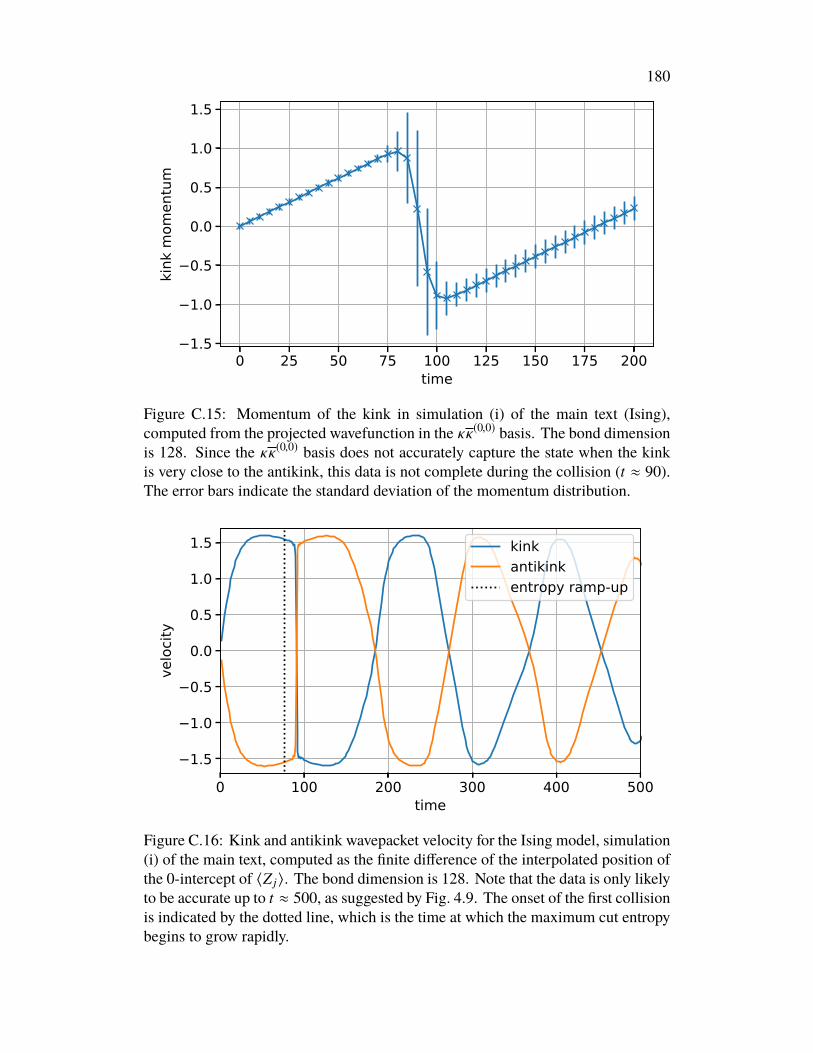
180

0 25 50 75 100 125 150 175 200time

1.5

1.0

0.5

0.0

0.5

1.0

1.5

kink

mom

entu

m

Figure C.15: Momentum of the kink in simulation (i) of the main text (Ising),computed from the projected wavefunction in the κκ(0,0) basis. The bond dimensionis 128. Since the κκ(0,0) basis does not accurately capture the state when the kinkis very close to the antikink, this data is not complete during the collision (t ≈ 90).The error bars indicate the standard deviation of the momentum distribution.

0 100 200 300 400 500time

1.5

1.0

0.5

0.0

0.5

1.0

1.5

velo

city

kinkantikinkentropy ramp-up

Figure C.16: Kink and antikink wavepacket velocity for the Ising model, simulation(i) of the main text, computed as the finite difference of the interpolated position ofthe 0-intercept of 〈Z j〉. The bond dimension is 128. Note that the data is only likelyto be accurate up to t ≈ 500, as suggested by Fig. 4.9. The onset of the first collisionis indicated by the dotted line, which is the time at which the maximum cut entropybegins to grow rapidly.

181

0 100 200 300 400 500time

1.5

1.0

0.5

0.0

0.5

1.0

1.5

velo

city

kinkantikinkentropy ramp-up

Figure C.17: Kink and antikink wavepacket velocity for simulation (ii), computedas the finite difference of the interpolated position of the 0-intercept of 〈Z j〉. Thebond dimension is 128. The interpretation of the 0-intercept as the position breaksdown both during and, to some extent, after the collision: During the collision,the zero intercept disappears altogether as the kink and antikink merge and all spinexpectation values are > 0. After the collision, there are in this case (see Fig. 4.8) atleast two different bubble "branches” of the wavefunction, both contributing to thespin expectation values. The onset of the first collision is indicated by the dottedline, which is the time at which the maximum cut entropy begins to grow rapidly.

returns to its vacuum value for p = 4π32 , suggesting a trivial scattering event (see

App. C.9). For p = 5π32 and p = 6π

32 , we observe a residual entropy surplus afterthe collision, suggesting nontrivial scattering. Since the onset of this extra entropycontribution coincides with the energy crossing the two-meson threshold 2mµ, it islikely due to an increasing probability of meson pair production.

It is interesting to note that, if we set h > 0 while keeping the other Hamiltonianparameters the same, we observe nontrivial, albeit elastic, scattering of kink-antikinkpairswhen the energy is below the two-meson threshold. Turning off the longitudinalfield appears to turn off this nontrivial elastic contribution, so that kinks and antikinksscatter trivially.

C.9 Entanglement generated by an elastic collisionHere we consider how two single-particle wavepackets become entangled whenthey scatter elastically in one spatial dimension. The entanglement arises from the

182

Figure C.18: Cut entropy for kink-antikink collisions, in the absence of a longi-tudinal field, with initial kink momentum p and antikink momentum −p, for threedifferent values of p. The Hamiltonian parameters are g = 0.9, λ = 0.3, h = 0,and the wavepacket width is σ = 19.0. The vacuum bond dimension is D = 14,with a limit D ≤ 64 imposed during evolution. The integration time-step size wasδt = 0.05.

momentum dependence of the scattering phase shift.

For this analysis we ignore lattice effects and consider two distinguishable particlesA and B propagating in the continuum. A pure state expanded in the momentumbasis has the form

|ψ〉 =

∫dpdq ψ(p, q)|p〉A |q〉B , (C.41)

with the normalization ∫dpdq |ψ(p, q)|2 = 1 . (C.42)

We assume the initial state factorizes as the product ψ(p, q) = ψA(p)ψB(q) of twowidely separated wavepackets, but after elastic scattering, the wave packets becomescorrelated due to the momentum dependent phase shift φ(p, q):

ψ(p, q) = ψA(p)ψB(q)eiφ(p,q) . (C.43)

183

Tracing out particle B, we obtain the reduced density matrix for particle A

ρA =

∫dp1dp2 |p1〉 ρA (p1, p2) 〈p2 | ,

ρA (p1, p2) =

∫dq ψ (p1, q)ψ∗ (p2, q) , (C.44)

where ∗ denotes complex conjugation.

To quantify the entanglement of particles A and B, we compute the Rényi entropiesof ρA,

Sn =1

1 − nlog2 ρ

nA , (C.45)

where

trρnA =

∫dp1dp2 . . . dpn dq1dq2 . . . dqn

|ψA(p1)|2 |ψA(p2)|

2 . . . |ψA(pn)|2 |ψB(q1)|

2 |ψB(q2)|2 . . . |ψB(qn)|

2

exp [i (φ(p1, q1) − φ(p2, q1) + φ(p2, q2) − φ(p3, q2) · · · + φ(pn, qn) − φ(p1, qn))] .

(C.46)

Now suppose that the wave packets for particles A and B are Gaussian:

|ψA(p)|2 =1

√2π∆A

e−(p−p)2/2∆2A ,

|ψB(q)|2 =1

√2π∆B

e−(q−q)2/2∆2B . (C.47)

If the phase shift were slowly varying over the range in p and q where the wavepackets have significant support, we could approximate trρn

A by expanding φ(p, q)to quadratic order about (p, q). But in that case the scattered wave packets are onlyslightly entangled. In order to do an analytic computation, we will assume thatφ(p, q) is exactly quadratic even if the phase shift varies rapidly. Then the only termthat matters is the cross term

φ(p, q) = φ2pq + . . . , (C.48)

because the exponential of the other terms factorizes into a function of p times afunction of q, which does not contribute to the entanglement of particles A and B.

By evaluating a Gaussian integral, we find

trρnA =

[n−1∏k=1

(1 + 4α2sin2

(kπn

))]−1/2

,

Sn =1

2(n − 1)

n−1∑k=1

log2

(1 + 4α2sin2

(kπn

)), (C.49)

184

where

α = φ2∆A∆B . (C.50)

Aswe anticipated, for |α | 1 the phase shift is rapidly varying and the entanglementis substantial. Using the formula

n−1∏k=1

4 sin2(

kπn

)= n2 (C.51)

we find

trρnA =

1n|α |n−1

(1 +O(α−2)

). (C.52)

We can extract the large-α behavior of the von Neumann entropy by taking the limit

S1 = tr ρA log2 ρA = limn→1

11 − n

log2 trρnA

≈ limn→1

(n − 1) log2 |α | + log2 nn − 1

= log2(e|α |). (C.53)

The entanglement entropy of particles A and B, after the elastic scattering event,scales like log |α |; therefore we expect to need a bond dimension scaling like |α | tosimulate the scattering process accurately using an MPS approximation.

In fact, by invoking properties of Chebyshev polynomials, the product over k in(C.49) can be evaluated explicitly, yielding [275]

Sn =1

2(n − 1)[1 + 2nlog2 |α | + log2(cosh(bn) − 1)

], (C.54)

where

b ≡ arccosh(1 +

12|α |2

). (C.55)

In the limit n→ 1 we find

S1 = log2 |α | +b2

(1 + 4|α |2

)1/2log2 e ; (C.56)

taking the large-α limit using arccosh(1 + x) =√

2x (1 +O(x)), we recover (C.53).

185

A p p e n d i x D

OTHER PUBLICATIONS

Other publications during the author’s graduate school that are related to this thesis.

A. Buser, H. Gharibyan, M. Hanada, M. Honda, J. Liu, Quantum simulation ofgauge theory via orbifold lattice, arxiv: 2011.06576 [hep-th].

H. Gharibyan, M. Hanada, M. Honda, J. Liu, Toward simulating Superstring/M-theory on a quantum computer, arxiv: 2011.06573 [hep-th].

Y.Z. Li, J. Liu, On Quantum Simulation Of Cosmic Inflation, arXiv:2009.10921[quant-ph].

J. Liu, D. Meltzer, D. Poland and D. Simmons-Duffin, The Lorentzian inver-sion formula and the spectrum of the 3d O(2) CFT, JHEP 09, 115 (2020),arXiv:2007.07914 [hep-th].

X. Yuan, J. Sun, J. Liu, Q. Zhao and Y. Zhou, Quantum simulation with hybridtensor networks, arXiv:2007.00958 [quant-ph].

J. Liu and Y. Xin, Quantum simulation of quantum field theories as quantum chem-istry, JHEP 12, 011 (2020), arXiv:2004.13234 [hep-th].

J. Liu, Scrambling and decoding the charged quantum information, Phys. Rev.Research 2, 043164 (2020), arXiv:2003.11425 [quant-ph].

S.M. Chester, W. Landry, J. Liu, D. Poland, D. Simmons-Duffin, N. Su andA. Vichi,Carving out OPE space and precise O(2) model critical exponents, JHEP 06,142 (2020), arXiv:1912.03324 [hep-th].

A. Lewkowycz, J. Liu, E. Silverstein and G. Torroba, TT and EE, with implicationsfor (A)dS subregion encodings, JHEP 04, 152 (2020), arXiv: 1909.13808[hep-th].

C. Cheung, J. Liu and G. N. Remmen, Entropy Bounds on Effective Field Theoryfrom Rotating Dyonic Black Holes, Phys. Rev. D 100, no. 4, 046003 (2019),arXiv:1903.09156 [hep-th].

J. Liu and Y. Zhou, Note on global symmetry and SYK model, JHEP 05, 099 (2019),arXiv:1901.05666 [hep-th].

N. Bao and J. Liu, Quantum algorithms for conformal bootstrap, Nucl. Phys. B946, 114702 (2019), arXiv:1811.05675 [hep-th].

186

J. Liu, E. Perlmutter, V. Rosenhaus and D. Simmons-Duffin, d-dimensional SYK,AdS Loops, and 6 j Symbols, JHEP 03, 052 (2019), arXiv:1808.00612 [hep-th].

J. Liu, Spectral form factors and late time quantum chaos, Phys. Rev. D 98, no.8,086026 (2018), arXiv:1806.05316 [hep-th].

N. Bao and J. Liu,Quantum complexity and the virial theorem, JHEP 08, 144 (2018),arXiv:1804.03242 [hep-th].

P. Kraus, J. Liu and D. Marolf, Cutoff AdS3 versus the TT deformation, JHEP 07,027 (2018), arXiv:1801.02714 [hep-th].

Y. Zhou and J. Liu, Note on the Green’s function formalism and topological invari-ants, J. Stat. Mech. 2003, no.3, 033101 (2020), arXiv:1712.08775 [hep-th]].

N. Hunter-Jones and J. Liu, Chaos and random matrices in supersymmetric SYK,JHEP 05, 202 (2018), arXiv:1710.08184 [hep-th].

N. Hunter-Jones, J. Liu and Y. Zhou, On thermalization in the SYK and supersym-metric SYK models, JHEP 02, 142 (2018), arXiv:1710.03012 [hep-th].

J. Liu, Artificial Neural Network in Cosmic Landscape, JHEP 12 (2017) 149,arXiv:1707.02800 [hep-th].

J. Cotler, N. Hunter-Jones, J. Liu and B. Yoshida, Chaos, Complexity, and RandomMatrices, JHEP 11, 048 (2017), arXiv:1706.05400 [hep-th].

T. Li, J. Liu, Y. Xin and Y. Zhou, Supersymmetric SYK model and random matrixtheory, JHEP 06, 111 (2017), arXiv:1702.01738 [hep-th].