Emerging Topics in Computer Vision
667
Emerging Topics in Computer Vision Edited by G´ erard Medioni and Sing Bing Kang
-
Upload
khangminh22 -
Category
Documents
-
view
1 -
download
0
Transcript of Emerging Topics in Computer Vision

Emerging Topics in
Computer Vision
Edited by
Gerard Medioni and Sing Bing Kang
Contents
PREFACE ix
CONTRIBUTORS x
1 INTRODUCTION 11.1 Organization 11.2 How to Use the Book 2
SECTION I:FUNDAMENTALS IN COMPUTER VISION 3
2 CAMERA CALIBRATION 5Zhengyou Zhang2.1 Introduction 52.2 Notation and Problem Statement 7
2.2.1 Pinhole Camera Model 82.2.2 Absolute Conic 9
2.3 Camera Calibration with 3D Objects 112.3.1 Feature Extraction 132.3.2 Linear Estimation of the Camera Projection Matrix 132.3.3 Recover Intrinsic and Extrinsic Parameters from P 142.3.4 Refine Calibration Parameters Through a Nonlinear
Optimization 152.3.5 Lens Distortion 152.3.6 An Example 17
2.4 Camera Calibration with 2D Objects: Plane Based Technique 182.4.1 Homography between the model plane and its image 182.4.2 Constraints on the intrinsic parameters 192.4.3 Geometric Interpretation2 192.4.4 Closed-form solution 202.4.5 Maximum likelihood estimation 22
i
ii Contents
2.4.6 Dealing with radial distortion 222.4.7 Summary 232.4.8 Experimental Results 242.4.9 Related Work 26
2.5 Solving Camera Calibration With 1D Objects 272.5.1 Setups With Free-Moving 1D Calibration Objects 282.5.2 Setups With 1D Calibration Objects Moving Around
a fixed Point 292.5.3 Basic Equations 302.5.4 Closed-Form Solution 322.5.5 Nonlinear Optimization 332.5.6 Estimating the fixed point 342.5.7 Experimental Results 35
2.6 Self Calibration 392.7 Conclusion 392.8 Appendix: Estimating Homography Between the Model Plane
and its Image 40Bibliography 41
3 MULTIPLE VIEW GEOMETRY 45Anders Heyden and Marc Pollefeys3.1 Introduction 453.2 Projective Geometry 46
3.2.1 The central perspective transformation 463.2.2 Projective spaces 473.2.3 Homogeneous coordinates 493.2.4 Duality 523.2.5 Projective transformations 54
3.3 Tensor Calculus 563.4 Modelling Cameras 58
3.4.1 The pinhole camera 583.4.2 The camera matrix 593.4.3 The intrinsic parameters 593.4.4 The extrinsic parameters 603.4.5 Properties of the pinhole camera 62
3.5 Multiple View Geometry 633.5.1 The structure and motion problem 633.5.2 The two-view case 643.5.3 Multi-view constraints and tensors 70
3.6 Structure and Motion I 75
Contents iii
3.6.1 Resection 753.6.2 Intersection 753.6.3 Linear estimation of tensors 763.6.4 Factorization 78
3.7 Structure and Motion II 803.7.1 Two-view geometry computation 803.7.2 Structure and motion recovery 83
3.8 Auto-calibration 873.9 Dense Depth Estimation 90
3.9.1 Rectification 903.9.2 Stereo matching 923.9.3 Multi-view linking 93
3.10 Visual Modeling 943.10.1 3D surface reconstruction 953.10.2 Image-based rendering 983.10.3 Match-moving 101
3.11 Conclusion 101Bibliography 103
4 ROBUST TECHNIQUES FOR COMPUTER VISION 109Peter Meer4.1 Robustness in Visual Tasks 1094.2 Models and Estimation Problems 113
4.2.1 Elements of a Model 1134.2.2 Estimation of a Model 1194.2.3 Robustness of an Estimator 1224.2.4 Definition of Robustness 1244.2.5 Taxonomy of Estimation Problems 1274.2.6 Linear Errors-in-Variables Regression Model 1304.2.7 Objective Function Optimization 134
4.3 Location Estimation 1394.3.1 Why Nonparametric Methods 1404.3.2 Kernel Density Estimation 1414.3.3 Adaptive Mean Shift 1464.3.4 Applications 150
4.4 Robust Regression 1574.4.1 Least Squares Family 1584.4.2 M-estimators 1634.4.3 Median Absolute Deviation Scale Estimate 1664.4.4 LMedS, RANSAC and Hough Transform 169

iv Contents
4.4.5 The pbM-estimator 1734.4.6 Applications 1784.4.7 Structured Outliers 180
4.5 Conclusion 183Bibliography 183
5 THE TENSOR VOTING FRAMEWORK 191Gerard Medioni and Philippos Mordohai5.1 Introduction 191
5.1.1 Motivation 1925.1.2 Desirable descriptions 1945.1.3 Our approach 1955.1.4 Chapter Overview 197
5.2 Related Work 1985.3 Tensor Voting in 2D 203
5.3.1 Second Order Representation and Voting in 2-D 2035.3.2 First Order Representation and Voting in 2-D 2105.3.3 Voting Fields 2135.3.4 Vote analysis 2155.3.5 Results in 2-D 2185.3.6 Illusory Contours 219
5.4 Tensor Voting in 3D 2215.4.1 Representation in 3-D 2225.4.2 Voting in 3-D 2245.4.3 Vote analysis 2265.4.4 Results in 3-D 228
5.5 Tensor Voting in ND 2295.5.1 Computational Complexity 232
5.6 Application to Computer Vision Problems 2335.6.1 Initial Matching 2345.6.2 Uniqueness 2355.6.3 Discrete Densification 2365.6.4 Discontinuity Localization 2375.6.5 Stereo 2395.6.6 Multiple View Stereo 2415.6.7 Visual Motion from Motion Cues 2435.6.8 Visual Motion on Real Images 245
5.7 Conclusion and Future Work 2465.8 Acknowledgment 250Bibliography 250
Contents v
SECTION II:APPLICATIONS IN COMPUTER VISION 254
6 IMAGE BASED LIGHTING 255Paul E. Debevec6.1 Basic Image Based Lighting 257
6.1.1 Capturing Light 2576.1.2 Illuminating Synthetic Objects with Real Light 2606.1.3 Lighting Entire Environments with IBL 269
6.2 Advanced Image Based Lighting 2696.2.1 Capturing a Light Probe in Direct Sunlight 2726.2.2 Compositing objects into the scene including shadows 2826.2.3 Image-Based Lighting in Fiat Lux 2886.2.4 Capturing and Rendering Spatially-Varying Illumination291
6.3 Image Based Relighting 2946.4 Conclusion 299Bibliography 301
7 COMPUTER VISION IN VISUAL EFFECTS 305Doug Roble7.1 Introduction 3057.2 Computer Vision Problems Unique to Film 306
7.2.1 Welcome to the Set 3067.3 Feature Tracking 3197.4 Optical Flow 3217.5 Camera Tracking and Structure from Motion 3257.6 The Future 330Bibliography 330
8 CONTENT BASED IMAGE RETRIEVAL: AN OVERVIEW 333Theo Gevers and Arnold W.M. Smeulders8.1 Overview of the chapter 3348.2 Image Domains 339
8.2.1 Search modes 3398.2.2 The sensory gap 3418.2.3 The semantic gap 3428.2.4 Discussion 343
8.3 Image Features 3448.3.1 Color 3458.3.2 Shape 348
vi Contents
8.3.3 Texture 3498.3.4 Discussion 352
8.4 Representation and Indexing 3528.4.1 Grouping data 3538.4.2 Features accumulation 3548.4.3 Feature accumulation and image partitioning 3578.4.4 Salient features 3588.4.5 Shape and object features 3598.4.6 Structure and lay-out 3618.4.7 Discussion 361
8.5 Similarity and Search 3628.5.1 Semantic interpretation 3628.5.2 Similarity between features 3638.5.3 Similarity of object outlines 3668.5.4 Similarity of object arrangements 3678.5.5 Similarity of salient features 3688.5.6 Discussion 369
8.6 Interaction and Learning 3698.6.1 Interaction on a semantic level 3698.6.2 Classification on a semantic level 3708.6.3 Learning 3718.6.4 Discussion 371
8.7 Conclusion 372Bibliography 372
9 FACE DETECTION, ALIGNMENT AND RECOGNITION 385Stan Z. Li and Juwei Lu9.1 Introduction 3859.2 Face Detection 388
9.2.1 Appearance and Learning Based Approach 3899.2.2 Preprocessing 3919.2.3 Neural and Kernel Methods 3939.2.4 Boosting Based Methods 3949.2.5 Post-Processing 4009.2.6 Evaluation 401
9.3 Face Alignment 4049.3.1 Active Shape Model 4059.3.2 Active Appearance Model 4079.3.3 Modeling Shape from Texture 4089.3.4 Dealing with Head Pose 414

Contents vii
9.3.5 Evaluation 4169.4 Face Recognition 419
9.4.1 Preprocessing 4199.4.2 Feature Extraction 4209.4.3 Pattern Classification 4319.4.4 Evaluation 439
Bibliography 445
10 PERCEPTUAL INTERFACES 455Matthew Turk and Mathias Kolsch10.1 Introduction 45510.2 Perceptual Interfaces and HCI 45710.3 Multimodal Interfaces 46410.4 Vision Based Interfaces 472
10.4.1 Terminology 47610.4.2 Elements of VBI 47910.4.3 Computer Vision Methods for VBI 49110.4.4 VBI Summary 504
10.5 Brain-Computer Interfaces 50410.6 Summary 507Bibliography 509
SECTION III:PROGRAMMING FOR COMPUTER VISION 520
11 OPEN SOURCE COMPUTER VISION LIBRARY 521Gary Bradski11.1 Overview 521
11.1.1 Installation 52211.1.2 Organization 52711.1.3 Optimizations 529
11.2 Functional Groups: What’s Good for What 53211.2.1 By Area 53411.2.2 By Task 53811.2.3 Demos and Samples 542
11.3 Pictorial Tour 54511.3.1 Functional Groups 54511.3.2 Demo Tour 561
11.4 Programming Examples Using C/C++ 56111.4.1 Read Images from Disk 566

viii Contents
11.4.2 Read AVIs from Disk, or Video from a Camera 56811.5 Other Interfaces 570
11.5.1 Ch 57011.5.2 Matlab 57511.5.3 Lush 577
11.6 Appendix A 57811.7 Appendix B 579Bibliography 580
12 SOFTWARE ARCHITECTURE FOR COMPUTER VI-SION 585Alexandre R.J. Francois12.1 Introduction 585
12.1.1 Motivation 58512.1.2 Contribution 58812.1.3 Outline 589
12.2 SAI: A Software Architecture Model 59012.2.1 Beyond Pipes and Filters 59012.2.2 The SAI Architectural Style 59712.2.3 Example Designs 60112.2.4 Architectural Properties 620
12.3 MFSM: An Architectural Middleware 62212.3.1 MFSM overview 62312.3.2 A First Image Manipulation Example 62612.3.3 Custom Elements 63412.3.4 A Shared Memory Access Example 643
12.4 Conclusion 64812.4.1 Summary 64812.4.2 Perspectives 649
12.5 Acknowledgments 651Bibliography 651
PREFACE
One of the major changes instituted at the 2001 Conference on ComputerVision and Pattern Recognition (CVPR) in Kauai, HI was the replacementof the traditional tutorial sessions with a set of short courses. The topicsof these short courses were carefully chosen to reflect the diversity in com-puter vision and represent very promising areas. The response to these shortcourses was a very pleasant surprise, with up to more than 200 people attend-ing a single short course. This overwhelming response was the inspirationfor this book.
There are three parts in this book. The first part covers some of the morefundamental aspects of computer vision, the second describes a few interest-ing applications, and third details specific approaches to facilitate program-ming for computer vision. This book is not intended to be a comprehensivecoverage of computer vision; it can, however, be used as a complement tomost computer vision textbooks.
A unique aspect of this book is the accompanying DVD which featuresvideos of lectures by the contributors. We feel that these lectures would bevery useful for readers as quick previews of the topics covered in the book.In addition, these lectures are much more effective in depicting results in theform of video or animations, compared to printed material.
We would like to thank all the contributors for all their hard work, andBernard Goodwin for his support and enthusiasm for our book project. TheUSC Distance Education Network helped to tape and produce the lecturesand Bertran Harden tirelessly assembled all the multimedia content onto aDVD. We are also grateful to P. Anandan and Microsoft Corporation for thefinancial support used to defray some of the lecture production costs.
Gerard Medioni, University of Southern CaliforniaSing Bing Kang, Microsoft ResearchNovember, 2003
ix

CONTRIBUTORS
Gary BradskiMgr: Machine Learning GroupIntel LabsSC12-3032200 Mission College Blvd.Santa Clara, CA 95052-8119USAwww.intel.com/research/mrl/research/opencvwww.intel.com/research/mrl/research/media-visual.htm
Paul DebevecUSC Institute for Creative Technologies13274 Fiji Way, 5th FloorMarina del Rey, CA 90292USAhttp://www.debevec.org/
Alexandre R.J. FrancoisPHE-222 MC-0273Institute for Robotics and Intelligent SystemsUniversity of Southern CaliforniaLos Angeles, CA [email protected]/ afrancoi
x

Contributors xi
Theo GeversUniversity of AmsterdamKruislaan 4031098 SJ AmsterdamThe [email protected]://carol.science.uva.nl/ gevers/
Anders HeydenCentre for Mathematical SciencesLund UniversityBox 118SE-221 00 [email protected]/matematiklth/personal/andersp/
Mathias KolschComputer Science DepartmentUniversity of CaliforniaSanta Barbara, CA [email protected]://www.cs.ucsb.edu/∼matz
Stan Z. LiMicrosoft Research Asia5/F, Beijing Sigma CenterNo. 49, Zhichun Road, Hai Dian DistrictBeijing, China [email protected]/∼szli
Juwei LuBell Canada Multimedia LabUniversity of TorontoBahen Centre for Information TechnologyRoom 4154, 40 St George Str.Toronto, ON, M5S [email protected]/∼juwei/

xii Contributors
Gerard MedioniSAL 300, MC-0781Computer Science DepartmentUniversity of Southern CaliforniaLos Angeles, CA [email protected]/home/iris/medioni/User.html
Peter MeerElectrical and Computer Engineering DepartmentRutgers University94 Brett RoadPiscataway, NJ [email protected]/∼meer
Philippos MordohaiPHE 204, MC-02733737 Watt WayLos Angeles, CA [email protected]/home/iris/mordohai/User.html
Marc PollefeysDepartment of Computer ScienceUniversity of North CarolinaSitterson Hall, CB#3175Chapel Hill, NC [email protected]/∼marc/
Doug RobleDigital Domain300 Rose AvVenice, CA 90291USAwww.d2.com

Contributors xiii
Arnold SmeuldersISIS group, University of AmsterdamKruislaan 4031098SJ AMSTERDAMThe [email protected]/isis/
Matthew TurkComputer Science DepartmentUniversity of CaliforniaSanta Barbara, CA [email protected]/∼mturk
Zhengyou ZhangMicrosoft CorporationOne Microsoft WayRedmond, WA [email protected]/∼zhang/
Chapter 1
INTRODUCTION
The topics in this book were handpicked to showcase what we consider tobe exciting and promising in computer vision. They are a mix of morewell-known and traditional topics (such as camera calibration, multi-viewgeometry, and face detection), and newer ones (such as vision for specialeffects and tensor voting framework). All have the common denominator ofeither demonstrated longevity or potential for endurance in computer vision,when the popularity of a number of areas have come and gone in the past.
1.1 Organization
The book is organized into three sections, covering various fundamentals,applications, and programming aspects of computer vision.
The fundamentals section consists of four chapters. Two of the chaptersdeal with the more conventional but still popular areas: camera calibrationand multi-view geometry. They deal with the most fundamental operationsassociated with vision. The chapter on robust estimation techniques will bevery useful for researchers and practitioners of computer vision alike. Thereis also a chapter on a more recent tool (namely the tensor voting framework)developed that can be customized for a variety of problems.
The applications section covers two more recent applications (image-based lighting and vision for visual effects) and three in more conventionalareas (image seach engines, face detection and recognition, and perceptualinterfaces).
One of the more overlooked area in computer vision is the programmingaspect of computer vision. While there are generic commercial packages thatcan be used, there exists popular libraries or packages that are specificallygeared for computer vision. The final section of the book describes twodifferent approaches to facilitate programming for computer vision.
1

2 Introduction Chapter 1
1.2 How to Use the Book
The book is designed to be accompanying material to computer vision text-books.
Each chapter is designed to be self-contained, and is written by well-known authorities in the area. We suggest that the reader watch the lecturefirst before reading the chapter, as the lecture (given by the contributor)provides an excellent overview of the topic.
SECTION I:FUNDAMENTALS INCOMPUTER VISION
It is only fitting that we start with some of the more fundamental conceptsin computer vision. The range of topics covered in this section is wide:camera calibration, structure from motion, dense stereo, 3D modeling, robusttechniques for model fitting, and a more recently developed concept calledtensor voting.
In Chapter 2, Zhang reviews the different techniques for calibrating acamera. More specifically, he describes calibration techniques that use 3Dreference objects, 2D planes, and 1D lines, as well as self-calibration tech-niques.
One of more popular (and difficult) areas in computer vision is stereo.Heyden and Pollefeys describe how camera motion and scene structure canbe reliably extracted from image sequences in Chapter 3. Once this is ac-complished, dense depth distributions can be extracted for 3D surface recon-struction and image-based rendering applications.
A basic task in computer vision is hypothesizing models (e.g., 2D shapes)and using input data (typically image data) to corroborate and fit the models.In practice, however, robust techniques for model fitting must be used tohandle input noise. In Chapter 4, Meer describes various robust regressiontechniques such as M-estimators, RANSAC, and Hough transform. He alsocovers the mean shift algorithm for the location estimation problem.
The claim by Medioni and his colleagues that computer vision problemscan be addressed within a Gestalt framework is the basis of their work ontensor voting. In Chapter 5, Medioni and Mordohai provide an introductionto the concept of tensor voting, which is a form of binning according to
3

4Section I:
Fundamentals in Computer Vision
proximity to ideal primitives such as edges and points. They show how thisscheme can be applied to a variety of applications, such as curve and surfaceextraction from noisy 2D and 3D points (respectively), stereo matching, andmotion-based grouping.
Chapter 2
CAMERA CALIBRATION
Zhengyou Zhang
Camera calibration is a necessary step in 3D computer vision in order toextract metric information from 2D images. It has been studied extensivelyin computer vision and photogrammetry, and even recently new techniqueshave been proposed. In this chapter, we review the techniques proposedin the literature include those using 3D apparatus (two or three planes or-thogonal to each other, or a plane undergoing a pure translation, etc.), 2Dobjects (planar patterns undergoing unknown motions), 1D objects (wandwith dots) and unknown scene points in the environment (self-calibration).The focus is on presenting these techniques within a consistent framework.
2.1 Introduction
Camera calibration is a necessary step in 3D computer vision in order toextract metric information from 2D images. Much work has been done,starting in the photogrammetry community (see [3, 6] to cite a few), andmore recently in computer vision ([12, 11, 33, 10, 37, 35, 22, 9] to cite a few).According to the dimension of the calibration objects, we can classify thosetechniques roughly into three categories.
3D reference object based calibration. Camera calibration is performedby observing a calibration object whose geometry in 3-D space is knownwith very good precision. Calibration can be done very efficiently [8].The calibration object usually consists of two or three planes orthog-onal to each other. Sometimes, a plane undergoing a precisely knowntranslation is also used [33], which equivalently provides 3D referencepoints. This approach requires an expensive calibration apparatus and
5
6 Camera Calibration Chapter 2
an elaborate setup.
2D plane based calibration. Techniques in this category requires to ob-serve a planar pattern shown at a few different orientations [42, 31].Different from Tsai’s technique [33], the knowledge of the plane motionis not necessary. Because almost anyone can make such a calibrationpattern by him/her-self, the setup is easier for camera calibration.
1D line based calibration. Calibration objects used in this category arecomposed of a set of collinear points [44]. As will be shown, a cameracan be calibrated by observing a moving line around a fixed point, suchas a string of balls hanging from the ceiling.
Self-calibration. Techniques in this category do not use any calibrationobject, and can be considered as 0D approach because only imagepoint correspondences are required. Just by moving a camera in astatic scene, the rigidity of the scene provides in general two con-straints [22, 21] on the cameras’ internal parameters from one cameradisplacement by using image information alone. Therefore, if imagesare taken by the same camera with fixed internal parameters, cor-respondences between three images are sufficient to recover both theinternal and external parameters which allow us to reconstruct 3-Dstructure up to a similarity [20, 17]. Although no calibration objectsare necessary, a large number of parameters need to be estimated, re-sulting in a much harder mathematical problem.
Other techniques exist: vanishing points for orthogonal directions [4, 19],and calibration from pure rotation [16, 30].
Before going further, I’d like to point out that no single calibration tech-nique is the best for all. It really depends on the situation a user needs todeal with. Following are my few recommendations:
– Calibration with apparatus vs. self-calibration. Whenever possible, ifwe can pre-calibrate a camera, we should do it with a calibration appa-ratus. Self-calibration cannot usually achieve an accuracy comparablewith that of pre-calibration because self-calibration needs to estimate alarge number of parameters, resulting in a much harder mathematicalproblem. When pre-calibration is impossible (e.g., scene reconstructionfrom an old movie), self-calibration is the only choice.
– Partial vs. full self-calibration. Partial self-calibration refers to thecase where only a subset of camera intrinsic parameters are to be cal-
Section 2.2. Notation and Problem Statement 7
ibrated. Along the same line as the previous recommendation, when-ever possible, partial self-calibration is preferred because the numberof parameters to be estimated is smaller. Take an example of 3D re-construction with a camera with variable focal length. It is preferableto pre-calibrate the pixel aspect ratio and the pixel skewness.
– Calibration with 3D vs. 2D apparatus. Highest accuracy can usually beobtained by using a 3D apparatus, so it should be used when accuracy isindispensable and when it is affordable to make and use a 3D apparatus.From the feedback I received from computer vision researchers andpractitioners around the world in the last couple of years, calibrationwith a 2D apparatus seems to be the best choice in most situationsbecause of its ease of use and good accuracy.
– Calibration with 1D apparatus. This technique is relatively new, and itis hard for the moment to predict how popular it will be. It, however,should be useful especially for calibration of a camera network. Tocalibrate the relative geometry between multiple cameras as well astheir intrinsic parameters, it is necessary for all involving cameras tosimultaneously observe a number of points. It is hardly possible toachieve this with 3D or 2D calibration apparatus1 if one camera ismounted in the front of a room while another in the back. This is nota problem for 1D objects. We can for example use a string of ballshanging from the ceiling.
This chapter is organized as follows. Section 2.2 describes the cameramodel and introduces the concept of the absolute conic which is importantfor camera calibration. Section 2.3 presents the calibration techniques usinga 3D apparatus. Section 2.4 describes a calibration technique by observing afreely moving planar pattern (2D object). Its extension for stereo calibrationis also addressed. Section 2.5 describes a relatively new technique which usesa set of collinear points (1D object). Section 2.6 briefly introduces the self-calibration approach and provides references for further reading. Section 2.7concludes the chapter with a discussion on recent work in this area.
2.2 Notation and Problem Statement
We start with the notation used in this chapter.
1An exception is when those apparatus are made transparent; then the cost would bemuch higher.
8 Camera Calibration Chapter 2
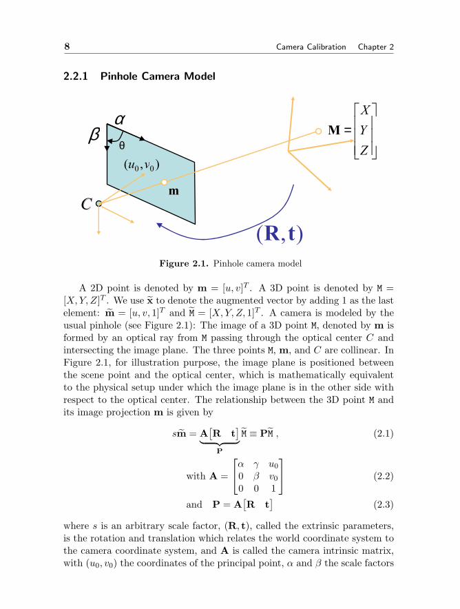
2.2.1 Pinhole Camera Model
CC
θθ
αβ
),( 00 vu
=ZYX
M
mm
),( tRFigure 2.1. Pinhole camera model
A 2D point is denoted by m = [u, v]T . A 3D point is denoted by M =[X,Y, Z]T . We use x to denote the augmented vector by adding 1 as the lastelement: m = [u, v, 1]T and M = [X,Y, Z, 1]T . A camera is modeled by theusual pinhole (see Figure 2.1): The image of a 3D point M, denoted by m isformed by an optical ray from M passing through the optical center C andintersecting the image plane. The three points M, m, and C are collinear. InFigure 2.1, for illustration purpose, the image plane is positioned betweenthe scene point and the optical center, which is mathematically equivalentto the physical setup under which the image plane is in the other side withrespect to the optical center. The relationship between the 3D point M andits image projection m is given by
sm = A[R t
]︸ ︷︷ ︸P
M ≡ PM , (2.1)
with A =
α γ u00 β v00 0 1
(2.2)
and P = A[R t
](2.3)
where s is an arbitrary scale factor, (R, t), called the extrinsic parameters,is the rotation and translation which relates the world coordinate system tothe camera coordinate system, and A is called the camera intrinsic matrix,with (u0, v0) the coordinates of the principal point, α and β the scale factors
Section 2.2. Notation and Problem Statement 9
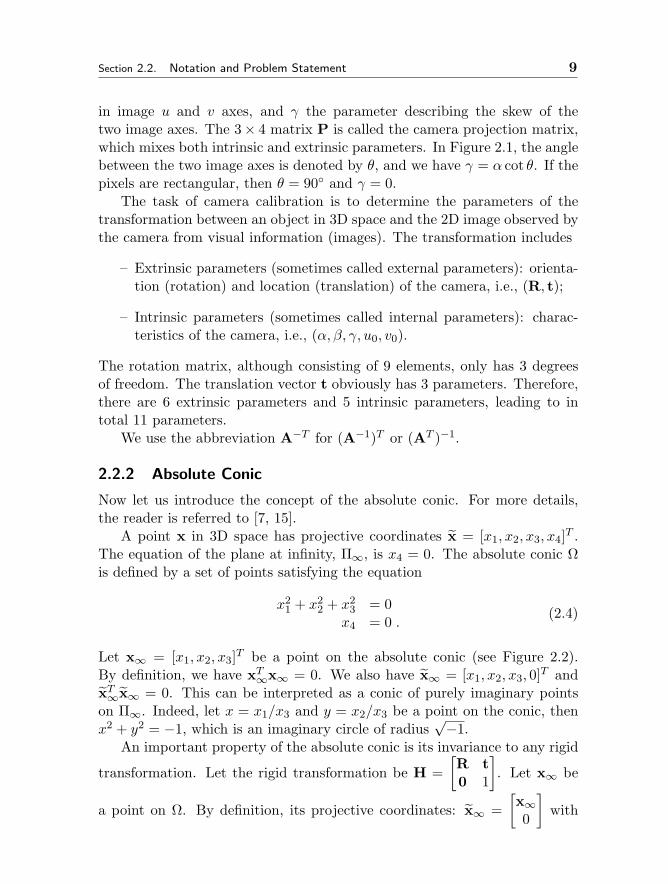
in image u and v axes, and γ the parameter describing the skew of thetwo image axes. The 3× 4 matrix P is called the camera projection matrix,which mixes both intrinsic and extrinsic parameters. In Figure 2.1, the anglebetween the two image axes is denoted by θ, and we have γ = α cot θ. If thepixels are rectangular, then θ = 90 and γ = 0.
The task of camera calibration is to determine the parameters of thetransformation between an object in 3D space and the 2D image observed bythe camera from visual information (images). The transformation includes
– Extrinsic parameters (sometimes called external parameters): orienta-tion (rotation) and location (translation) of the camera, i.e., (R, t);
– Intrinsic parameters (sometimes called internal parameters): charac-teristics of the camera, i.e., (α, β, γ, u0, v0).
The rotation matrix, although consisting of 9 elements, only has 3 degreesof freedom. The translation vector t obviously has 3 parameters. Therefore,there are 6 extrinsic parameters and 5 intrinsic parameters, leading to intotal 11 parameters.
We use the abbreviation A−T for (A−1)T or (AT )−1.
2.2.2 Absolute Conic
Now let us introduce the concept of the absolute conic. For more details,the reader is referred to [7, 15].
A point x in 3D space has projective coordinates x = [x1, x2, x3, x4]T .The equation of the plane at infinity, Π∞, is x4 = 0. The absolute conic Ωis defined by a set of points satisfying the equation
x21 + x2
2 + x23 = 0x4 = 0 .
(2.4)
Let x∞ = [x1, x2, x3]T be a point on the absolute conic (see Figure 2.2).By definition, we have xT∞x∞ = 0. We also have x∞ = [x1, x2, x3, 0]T andxT∞x∞ = 0. This can be interpreted as a conic of purely imaginary pointson Π∞. Indeed, let x = x1/x3 and y = x2/x3 be a point on the conic, thenx2 + y2 = −1, which is an imaginary circle of radius
√−1.An important property of the absolute conic is its invariance to any rigid
transformation. Let the rigid transformation be H =[R t0 1
]. Let x∞ be
a point on Ω. By definition, its projective coordinates: x∞ =[x∞0
]with

10 Camera Calibration Chapter 2
Plane at infinity
01 =∞−−
∞ mAAm TT
C
∞m
∞x
Absolute Conic
0=∞∞xxT
Image of Absolute Conic
Figure 2.2. Absolute conic and its image
xT∞x∞ = 0. The point after the rigid transformation is denoted by x′∞, and
x′∞ = Hx∞ =
[Rx∞
0
].
Thus, x′∞ is also on the plane at infinity. Furthermore, x′∞ is on the sameΩ because
x′T∞x′
∞ = (Rx∞)T (Rx∞) = xT∞(RTR)x∞ = 0 .
The image of the absolute conic, denoted by ω, is also an imaginary conic,and is determined only by the intrinsic parameters of the camera. This canbe seen as follows. Consider the projection of a point x∞ on Ω, denoted by
Section 2.3. Camera Calibration with 3D Objects 11
m∞, which is given by
m∞ = sA[R t][x∞0
]= sARx∞ .
It follows that
mTA−TA−1m = s2xT∞RTRx∞ = s2xT∞x∞ = 0 .
Therefore, the image of the absolute conic is an imaginary conic, and isdefined by A−TA−1. It does not depend on the extrinsic parameters of thecamera.
If we can determine the image of the absolute conic, then we can solvethe camera’s intrinsic parameters, and the calibration is solved.
We will show several ways in this chapter how to determine ω, the imageof the absolute conic.
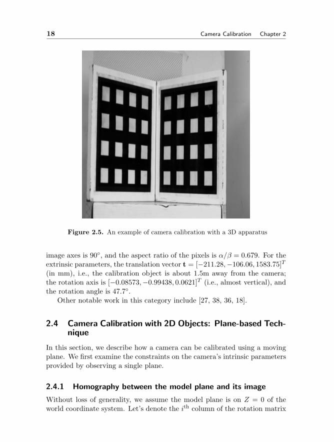
2.3 Camera Calibration with 3D Objects
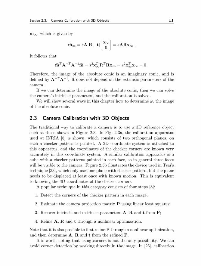
The traditional way to calibrate a camera is to use a 3D reference objectsuch as those shown in Figure 2.3. In Fig. 2.3a, the calibration apparatusused at INRIA [8] is shown, which consists of two orthogonal planes, oneach a checker pattern is printed. A 3D coordinate system is attached tothis apparatus, and the coordinates of the checker corners are known veryaccurately in this coordinate system. A similar calibration apparatus is acube with a checker patterns painted in each face, so in general three faceswill be visible to the camera. Figure 2.3b illustrates the device used in Tsai’stechnique [33], which only uses one plane with checker pattern, but the planeneeds to be displaced at least once with known motion. This is equivalentto knowing the 3D coordinates of the checker corners.
A popular technique in this category consists of four steps [8]:
1. Detect the corners of the checker pattern in each image;
2. Estimate the camera projection matrix P using linear least squares;
3. Recover intrinsic and extrinsic parameters A, R and t from P;
4. Refine A, R and t through a nonlinear optimization.
Note that it is also possible to first refine P through a nonlinear optimization,and then determine A, R and t from the refined P.
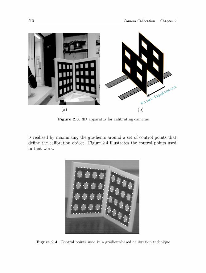
It is worth noting that using corners is not the only possibility. We canavoid corner detection by working directly in the image. In [25], calibration
12 Camera Calibration Chapter 2
Know
n disp
lacem
ent
Know
n disp
lacem
ent
(a) (b)
Figure 2.3. 3D apparatus for calibrating cameras
is realized by maximizing the gradients around a set of control points thatdefine the calibration object. Figure 2.4 illustrates the control points usedin that work.
Figure 2.4. Control points used in a gradient-based calibration technique

Section 2.3. Camera Calibration with 3D Objects 13
2.3.1 Feature Extraction
If one uses a generic corner detector, such as Harris corner detector, to detectthe corners in the check pattern image, the result is usually not good becausethe detector corners have poor accuracy (about one pixel). A better solutionis to leverage the known pattern structure by first estimating a line for eachside of the square and then computing the corners by intersecting the fittedlines. There are two common techniques to estimate the lines. The first is tofirst detect edges, and then fit a line to the edges on each side of the square.The second technique is to directly fit a line to each side of a square in theimage such that the gradient on the line is maximized. One possibility is torepresent the line by an elongated Gaussian, and estimate the parametersof the elongated Gaussian by maximizing the total gradient covered by theGaussian. We should note that if the lens distortion is not severe, a bettersolution is to fit just one single line to all the collinear sides. This will leadsa much more accurate estimation of the position of the checker corners.
2.3.2 Linear Estimation of the Camera Projection Matrix
Once we extract the corner points in the image, we can easily establish theircorrespondences with the points in the 3D space because of knowledge ofthe patterns. Based on the projection equation (2.1), we are now able toestimate the camera parameters. However, the problem is quite nonlinear ifwe try to estimate directly A, R and t. If, on the other hand, we estimatethe camera projection matrix P, a linear solution is possible, as to be shownnow.
Given each 2D-3D correspondence mi = (ui, vi) ↔ Mi = (Xi, Yi, Zi), wecan write down 2 equations based on (2.1):[
Xi Yi Zi 1 0 0 0 0 uiXi uiYi uiZi ui0 0 0 0 Xi Yi Zi 1 viXi viYi viZi vi
]︸ ︷︷ ︸
Gi
p = 0
where p = [p11, p12, . . . , p34]T and 0 = [0, 0]T .For n point matches, we can stack all equations together:
Gp = 0 with G = [GT1 , . . . ,G
Tn ]T
Matrix G is a 2n× 12 matrix. The projection matrix can now be solved by
minp‖Gp‖2 subject to ‖p‖ = 1
14 Camera Calibration Chapter 2
The solution is the eigenvector of GTG associated with the smallest eigen-value.
In the above, in order to avoid the trivial solution p = 0 and consideringthe fact that p is defined up to a scale factor, we have set ‖p‖ = 1. Othernormalizations are possible. In [1], p34 = 1, which, however, introduce a sin-gularity when the correct value of p34 is close to zero. In [10], the constraintp231 + p2
32 + p233 = 1 was used, which is singularity free.
Anyway, the above linear technique minimizes an algebraic distance, andyields a biased estimation when data are noisy. We will present later anunbiased solution.
2.3.3 Recover Intrinsic and Extrinsic Parameters from P
Once the camera projection matrix P is known, we can uniquely recover theintrinsic and extrinsic parameters of the camera. Let us denote the first 3×3submatrix of P by B and the last column of P by b, i.e., P ≡ [B b]. SinceP = A[R t], we have
B = AR (2.5)b = At (2.6)
From (2.5), we have
K ≡ BBT = AAT =
α2 + γ2 + u2
0︸ ︷︷ ︸ku
u0 v0 + c β︸ ︷︷ ︸kc
u0
u0 v0 + c α︸ ︷︷ ︸kc
α2v + v2
0︸ ︷︷ ︸kv
v0
u0 v0 1
Because P is defined up to a scale factor, the last element of K = BBT is usu-ally not equal to 1, so we have to normalize it such that K33(the last element) =1. After that, we immediately obtain
u0 = K13 (2.7)v0 = K23 (2.8)
β =√kv − v2
0 (2.9)
γ =kc − u0 v0
β(2.10)
α =√ku − u2
0 − γ2 (2.11)
Section 2.3. Camera Calibration with 3D Objects 15
The solution is unambiguous because: α > 0 and β > 0.Once the intrinsic parameters, or equivalently matrix A, are known, the
extrinsic parameters can be determined from (2.5) and (2.6) as:
R = A−1B (2.12)
t = A−1b . (2.13)
2.3.4 Refine Calibration Parameters Through a Nonlinear Opti-mization
The above solution is obtained through minimizing an algebraic distancewhich is not physically meaningful. We can refine it through maximumlikelihood inference.
We are given n 2D-3D correspondences mi = (ui, vi)↔ Mi = (Xi, Yi, Zi).Assume that the image points are corrupted by independent and identicallydistributed noise. The maximum likelihood estimate can be obtained byminimizing the distances between the image points and their predicted po-sitions, i.e.,
minP
∑i
‖mi − φ(P, Mi)‖2 (2.14)
where φ(P, Mi) is the projection of Mi onto the image according to (2.1).This is a nonlinear minimization problem, which can be solved with the
Levenberg-Marquardt Algorithm as implemented in Minpack [23]. It requiresan initial guess of P which can be obtained using the linear technique de-scribed earlier. Note that since P is defined up to a scale factor, we can setthe element having the largest initial value as 1 during the minimization.
Alternatively, instead of estimating P as in (2.14), we can directly esti-mate the intrinsic and extrinsic parameters, A, R, and t, using the samecriterion. The rotation matrix can be parameterized with three variablessuch as Euler angles or scaled rotation vector.
2.3.5 Lens Distortion
Up to this point, we use the pinhole model to describe a camera. It saysthat the point in 3D space, its corresponding point in image and the camera’soptical center are collinear. This linear projective equation is sometimes notsufficient, especially for low-end cameras (such as WebCams) or wide-anglecameras; lens distortion has to be considered.
According to [33], there are four steps in camera projection including lensdistortion:
16 Camera Calibration Chapter 2
Step 1: Rigid transformation from world coordinate system (Xw, Yw, Zw)to camera one (X,Y, Z):
[X Y Z]T = R [Xw Yw Zw]T + t
Step 2: Perspective projection from 3D camera coordinates (X,Y, Z) toideal image coordinates (x, y) under pinhole camera model:
x = fX
Z, y = f
Y
Z
where f is the effective focal length.
Step 3: Lens distortion2:
x = x+ δx , y = y + δy
where (x, y) are the distorted or true image coordinates, and (δx, δy)are distortions applied to (x, y).
Step 4: Affine transformation from real image coordinates (x, y) to framebuffer (pixel) image coordinates (u, v):
u = d−1x x+ u0 , v = d−1
y y + v0 ,
where (u0, v0) are coordinates of the principal point; dx and dy are dis-tances between adjacent pixels in the horizontal and vertical directions,respectively.
There are two types of distortions:
Radial distortion: It is symmetric; ideal image points are distorted alongradial directions from the distortion center. This is caused by imperfectlens shape.
Decentering distortion: This is usually caused by improper lens assem-bly; ideal image points are distorted in both radial and tangential di-rections.
The reader is referred to [29, 3, 6, 37] for more details.2Note that the lens distortion described here is different from Tsai’s treatment. Here,
we go from ideal to real image coordinates, similar to [36].
Section 2.3. Camera Calibration with 3D Objects 17
The distortion can be expressed as power series in radial distance r =√x2 + y2:
δx = x(k1r2 + k2r
4 + k3r6 + · · · ) + [p1(r2 + 2x2) + 2p2xy](1 + p3r
2 + · · · ) ,δy = y(k1r
2 + k2r4 + k3r
6 + · · · ) + [2p1xy + p2(r2 + 2y2)](1 + p3r2 + · · · ) ,
where ki’s are coefficients of radial distortion and pj ’s and coefficients ofdecentering distortion.
Based on the reports in the literature [3, 33, 36], it is likely that thedistortion function is totally dominated by the radial components, and es-pecially dominated by the first term. It has also been found that any moreelaborated modeling not only would not help (negligible when compared withsensor quantization), but also would cause numerical instability [33, 36].
Denote the ideal pixel image coordinates by u = x/dx, and v = y/dy. Bycombining Step 3 and Step 4 and if only using the first two radial distortionterms, we obtain the following relationship between (u, v) and (u, v):
u = u+ (u− u0)[k1(x2 + y2) + k2(x2 + y2)2] (2.15)
v = v + (v − v0)[k1(x2 + y2) + k2(x2 + y2)2] . (2.16)
Following the same reasoning as in (2.14), camera calibration includinglens distortion can be performed by minimizing the distances between theimage points and their predicted positions, i.e.,
minA,R,t,k1,k2
∑i
‖mi − m(A,R, t, k1, k2, Mi)‖2 (2.17)
where m(A,R, t, k1, k2, Mi) is the projection of Mi onto the image accordingto (2.1), followed by distortion according to (2.15) and (2.16).
2.3.6 An Example
Figure 2.5 displays an image of a 3D reference object, taken by a camera tobe calibrated at INRIA. Each square has 4 corners, and there are in total128 points used for calibration.
Without considering lens distortion, the estimated camera projection ma-trix is
P =
7.025659e−01 −2.861189e−02 −5.377696e−01 6.241890e+012.077632e−01 1.265804e+00 1.591456e−01 1.075646e+014.634764e−04 −5.282382e−05 4.255347e−04 1
From P, we can calculate the intrinsic parameters: α = 1380.12, β =2032.57, γ ≈ 0, u0 = 246.52, and v0 = 243.68. So, the angle between the two
18 Camera Calibration Chapter 2
Figure 2.5. An example of camera calibration with a 3D apparatus
image axes is 90, and the aspect ratio of the pixels is α/β = 0.679. For theextrinsic parameters, the translation vector t = [−211.28,−106.06, 1583.75]T
(in mm), i.e., the calibration object is about 1.5m away from the camera;the rotation axis is [−0.08573,−0.99438, 0.0621]T (i.e., almost vertical), andthe rotation angle is 47.7.
Other notable work in this category include [27, 38, 36, 18].
2.4 Camera Calibration with 2D Objects: Plane-based Tech-nique
In this section, we describe how a camera can be calibrated using a movingplane. We first examine the constraints on the camera’s intrinsic parametersprovided by observing a single plane.
2.4.1 Homography between the model plane and its image
Without loss of generality, we assume the model plane is on Z = 0 of theworld coordinate system. Let’s denote the ith column of the rotation matrix
Section 2.4. Camera Calibration with 2D Objects: Plane Based Technique 19
R by ri. From (2.1), we have
s
uv1
= A[r1 r2 r3 t
] XY01
= A[r1 r2 t
] XY1
.
By abuse of notation, we still use M to denote a point on the model plane, butM = [X,Y ]T since Z is always equal to 0. In turn, M = [X,Y, 1]T . Therefore,a model point M and its image m is related by a homography H:
sm = HM with H = A[r1 r2 t
]. (2.18)
As is clear, the 3× 3 matrix H is defined up to a scale factor.
2.4.2 Constraints on the intrinsic parameters
Given an image of the model plane, an homography can be estimated (seeAppendix). Let’s denote it by H = [h1 h2 h3]. From (2.18), we have
[h1 h2 h3] = λA [ r1 r2 t ] ,
where λ is an arbitrary scalar. Using the knowledge that r1 and r2 areorthonormal, we have
hT1 A−TA−1h2 = 0 (2.19)
hT1 A−TA−1h1 = hT2 A−TA−1h2 . (2.20)
These are the two basic constraints on the intrinsic parameters, given onehomography. Because a homography has 8 degrees of freedom and thereare 6 extrinsic parameters (3 for rotation and 3 for translation), we can onlyobtain 2 constraints on the intrinsic parameters. Note that A−TA−1 actuallydescribes the image of the absolute conic [20]. In the next subsection, wewill give an geometric interpretation.
2.4.3 Geometric Interpretation
We are now relating (2.19) and (2.20) to the absolute conic [22, 20].It is not difficult to verify that the model plane, under our convention, is
described in the camera coordinate system by the following equation:
[r3rT3 t
]T xyzw
= 0 ,
20 Camera Calibration Chapter 2
where w = 0 for points at infinity and w = 1 otherwise. This plane intersects
the plane at infinity at a line, and we can easily see that[r10
]and
[r20
]are
two particular points on that line. Any point on it is a linear combinationof these two points, i.e.,
x∞ = a
[r10
]+ b
[r20
]=[ar1 + br2
0
].
Now, let’s compute the intersection of the above line with the absoluteconic. By definition, the point x∞, known as the circular point [26], satisfies:xT∞x∞ = 0, i.e., (ar1 + br2)T (ar1 + br2) = 0, or a2 + b2 = 0 . The solutionis b = ±ai, where i2 = −1. That is, the two intersection points are
x∞ = a
[r1 ± ir2
0
].
The significance of this pair of complex conjugate points lies in the fact thatthey are invariant to Euclidean transformations. Their projection in theimage plane is given, up to a scale factor, by
m∞ = A(r1 ± ir2) = h1 ± ih2 .
Point m∞ is on the image of the absolute conic, described by A−TA−1 [20].This gives
(h1 ± ih2)TA−TA−1(h1 ± ih2) = 0 .
Requiring that both real and imaginary parts be zero yields (2.19) and (2.20).
2.4.4 Closed-form solution
We now provide the details on how to effectively solve the camera calibrationproblem. We start with an analytical solution. This initial estimation willbe followed by a nonlinear optimization technique based on the maximumlikelihood criterion, to be described in the next subsection.
Let
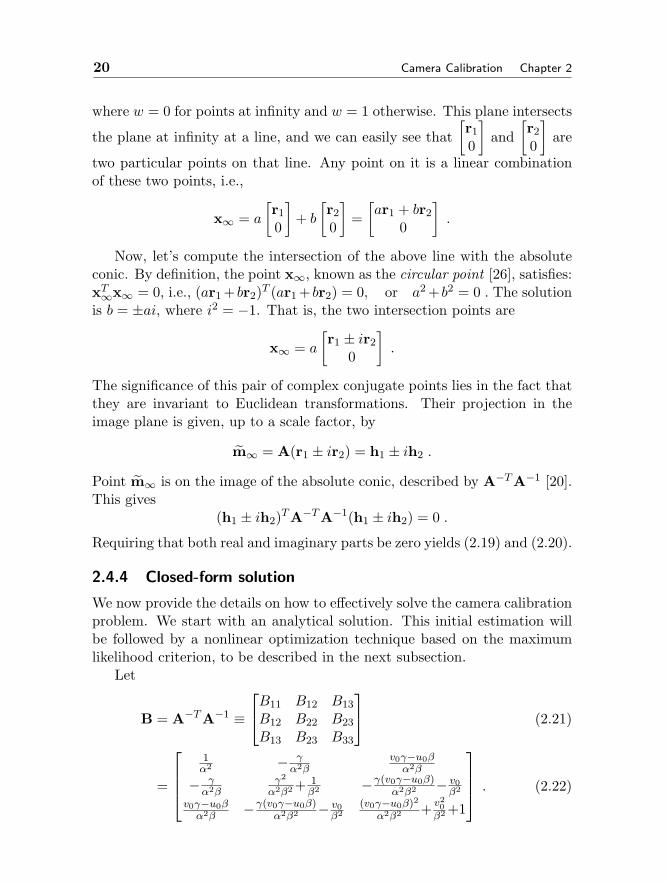
B = A−TA−1 ≡B11 B12 B13B12 B22 B23B13 B23 B33
(2.21)
=
1α2 − γ
α2βv0γ−u0βα2β
− γα2β
γ2
α2β2 + 1β2 −γ(v0γ−u0β)
α2β2 − v0β2
v0γ−u0βα2β
−γ(v0γ−u0β)α2β2 − v0
β2(v0γ−u0β)2
α2β2 + v20β2 +1
. (2.22)
Section 2.4. Camera Calibration with 2D Objects: Plane Based Technique 21
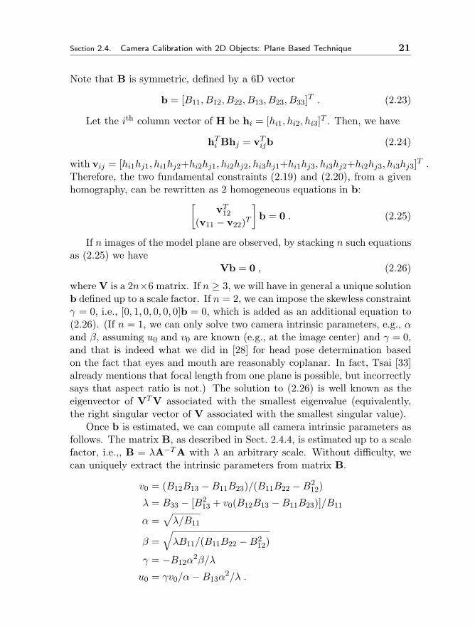
Note that B is symmetric, defined by a 6D vector
b = [B11, B12, B22, B13, B23, B33]T . (2.23)
Let the ith column vector of H be hi = [hi1, hi2, hi3]T . Then, we have
hTi Bhj = vTijb (2.24)
with vij = [hi1hj1, hi1hj2+hi2hj1, hi2hj2, hi3hj1+hi1hj3, hi3hj2+hi2hj3, hi3hj3]T .Therefore, the two fundamental constraints (2.19) and (2.20), from a givenhomography, can be rewritten as 2 homogeneous equations in b:[
vT12(v11 − v22)T
]b = 0 . (2.25)
If n images of the model plane are observed, by stacking n such equationsas (2.25) we have
Vb = 0 , (2.26)
where V is a 2n×6 matrix. If n ≥ 3, we will have in general a unique solutionb defined up to a scale factor. If n = 2, we can impose the skewless constraintγ = 0, i.e., [0, 1, 0, 0, 0, 0]b = 0, which is added as an additional equation to(2.26). (If n = 1, we can only solve two camera intrinsic parameters, e.g., αand β, assuming u0 and v0 are known (e.g., at the image center) and γ = 0,and that is indeed what we did in [28] for head pose determination basedon the fact that eyes and mouth are reasonably coplanar. In fact, Tsai [33]already mentions that focal length from one plane is possible, but incorrectlysays that aspect ratio is not.) The solution to (2.26) is well known as theeigenvector of VTV associated with the smallest eigenvalue (equivalently,the right singular vector of V associated with the smallest singular value).
Once b is estimated, we can compute all camera intrinsic parameters asfollows. The matrix B, as described in Sect. 2.4.4, is estimated up to a scalefactor, i.e.,, B = λA−TA with λ an arbitrary scale. Without difficulty, wecan uniquely extract the intrinsic parameters from matrix B.
v0 = (B12B13 −B11B23)/(B11B22 −B212)
λ = B33 − [B213 + v0(B12B13 −B11B23)]/B11
α =√λ/B11
β =√λB11/(B11B22 −B2
12)
γ = −B12α2β/λ
u0 = γv0/α−B13α2/λ .
22 Camera Calibration Chapter 2
Once A is known, the extrinsic parameters for each image is readilycomputed. From (2.18), we have
r1 = λA−1h1 , r2 = λA−1h2 , r3 = r1 × r2 , t = λA−1h3
with λ = 1/‖A−1h1‖ = 1/‖A−1h2‖. Of course, because of noise in data, theso-computed matrix R = [r1, r2, r3] does not in general satisfy the propertiesof a rotation matrix. The best rotation matrix can then be obtained throughfor example singular value decomposition [13, 41].
2.4.5 Maximum likelihood estimation
The above solution is obtained through minimizing an algebraic distancewhich is not physically meaningful. We can refine it through maximumlikelihood inference.
We are given n images of a model plane and there are m points on themodel plane. Assume that the image points are corrupted by independentand identically distributed noise. The maximum likelihood estimate can beobtained by minimizing the following functional:
n∑i=1
m∑j=1
‖mij − m(A,Ri, ti, Mj)‖2 , (2.27)
where m(A,Ri, ti, Mj) is the projection of point Mj in image i, according toequation (2.18). A rotation R is parameterized by a vector of 3 parameters,denoted by r, which is parallel to the rotation axis and whose magnitude isequal to the rotation angle. R and r are related by the Rodrigues formula [8].Minimizing (2.27) is a nonlinear minimization problem, which is solved withthe Levenberg-Marquardt Algorithm as implemented in Minpack [23]. Itrequires an initial guess of A, Ri, ti|i = 1..n which can be obtained usingthe technique described in the previous subsection.
Desktop cameras usually have visible lens distortion, especially the ra-dial components. We have included these while minimizing (2.27). See mytechnical report [41] for more details.
2.4.6 Dealing with radial distortion
Up to now, we have not considered lens distortion of a camera. However, adesktop camera usually exhibits significant lens distortion, especially radialdistortion. The reader is referred to Section 2.3.5 for distortion modeling.In this section, we only consider the first two terms of radial distortion.
Section 2.4. Camera Calibration with 2D Objects: Plane Based Technique 23
Estimating Radial Distortion by Alternation. As the radial distortion is ex-pected to be small, one would expect to estimate the other five intrinsicparameters, using the technique described in Sect. 2.4.5, reasonable well bysimply ignoring distortion. One strategy is then to estimate k1 and k2 afterhaving estimated the other parameters, which will give us the ideal pixelcoordinates (u, v). Then, from (2.15) and (2.16), we have two equations foreach point in each image:[
(u−u0)(x2+y2) (u−u0)(x2+y2)2
(v−v0)(x2+y2) (v−v0)(x2+y2)2
] [k1k2
]=[u−uv−v
].
Given m points in n images, we can stack all equations together to obtainin total 2mn equations, or in matrix form as Dk = d, where k = [k1, k2]T .The linear least-squares solution is given by
k = (DTD)−1DTd . (2.28)
Once k1 and k2 are estimated, one can refine the estimate of the other param-eters by solving (2.27) with m(A,Ri, ti, Mj) replaced by (2.15) and (2.16).We can alternate these two procedures until convergence.
Complete Maximum Likelihood Estimation. Experimentally, we found theconvergence of the above alternation technique is slow. A natural extensionto (2.27) is then to estimate the complete set of parameters by minimizingthe following functional:
n∑i=1
m∑j=1
‖mij − m(A, k1, k2,Ri, ti, Mj)‖2 , (2.29)
where m(A, k1, k2,Ri, ti, Mj) is the projection of point Mj in image i ac-cording to equation (2.18), followed by distortion according to (2.15) and(2.16). This is a nonlinear minimization problem, which is solved with theLevenberg-Marquardt Algorithm as implemented in Minpack [23]. A rota-tion is again parameterized by a 3-vector r, as in Sect. 2.4.5. An initial guessof A and Ri, ti|i = 1..n can be obtained using the technique described inSect. 2.4.4 or in Sect. 2.4.5. An initial guess of k1 and k2 can be obtained withthe technique described in the last paragraph, or simply by setting them to0.
2.4.7 Summary
The recommended calibration procedure is as follows:
24 Camera Calibration Chapter 2
1. Print a pattern and attach it to a planar surface;
2. Take a few images of the model plane under different orientations bymoving either the plane or the camera;
3. Detect the feature points in the images;
4. Estimate the five intrinsic parameters and all the extrinsic parametersusing the closed-form solution as described in Sect. 2.4.4;
5. Estimate the coefficients of the radial distortion by solving the linearleast-squares (2.28);
6. Refine all parameters, including lens distortion parameters, by mini-mizing (2.29).
There is a degenerate configuration in my technique when planes areparallel to each other. See my technical report [41] for a more detaileddescription.
In summary, this technique only requires the camera to observe a planarpattern from a few different orientations. Although the minimum numberof orientations is two if pixels are square, we recommend 4 or 5 differentorientations for better quality. We can move either the camera or the planarpattern. The motion does not need to be known, but should not be a puretranslation. When the number of orientations is only 2, one should avoidpositioning the planar pattern parallel to the image plane. The pattern couldbe anything, as long as we know the metric on the plane. For example, wecan print a pattern with a laser printer and attach the paper to a reasonableplanar surface such as a hard book cover. We can even use a book with knownsize because the four corners are enough to estimate the plane homographies.
2.4.8 Experimental Results
The proposed algorithm has been tested on both computer simulated dataand real data. The closed-form solution involves finding a singular valuedecomposition of a small 2n × 6 matrix, where n is the number of images.The nonlinear refinement within the Levenberg-Marquardt algorithm takes3 to 5 iterations to converge. Due to space limitation, we describe in thissection one set of experiments with real data when the calibration patternis at different distances from the camera. The reader is referred to [41] formore experimental results with both computer simulated and real data, andto the following Web page:
Section 2.4. Camera Calibration with 2D Objects: Plane Based Technique 25
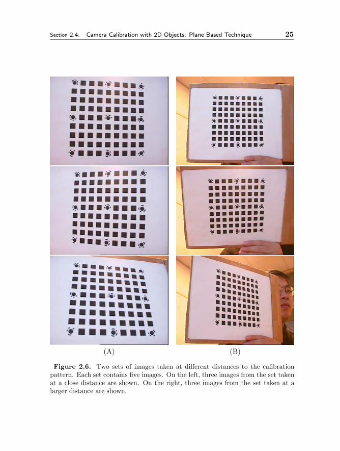
(A) (B)
Figure 2.6. Two sets of images taken at different distances to the calibrationpattern. Each set contains five images. On the left, three images from the set takenat a close distance are shown. On the right, three images from the set taken at alarger distance are shown.
26 Camera Calibration Chapter 2
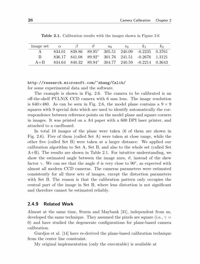
Table 2.1. Calibration results with the images shown in Figure 2.6
image set α β ϑ u0 v0 k1 k2
A 834.01 839.86 89.95 305.51 240.09 -0.2235 0.3761B 836.17 841.08 89.92 301.76 241.51 -0.2676 1.3121
A+B 834.64 840.32 89.94 304.77 240.59 -0.2214 0.3643
http://research.microsoft.com/˜zhang/Calib/for some experimental data and the software.
The example is shown in Fig. 2.6. The camera to be calibrated is anoff-the-shelf PULNiX CCD camera with 6 mm lens. The image resolutionis 640×480. As can be seen in Fig. 2.6, the model plane contains a 9 × 9squares with 9 special dots which are used to identify automatically the cor-respondence between reference points on the model plane and square cornersin images. It was printed on a A4 paper with a 600 DPI laser printer, andattached to a cardboard.
In total 10 images of the plane were taken (6 of them are shown inFig. 2.6). Five of them (called Set A) were taken at close range, while theother five (called Set B) were taken at a larger distance. We applied ourcalibration algorithm to Set A, Set B, and also to the whole set (called SetA+B). The results are shown in Table 2.1. For intuitive understanding, weshow the estimated angle between the image axes, ϑ, instead of the skewfactor γ. We can see that the angle ϑ is very close to 90, as expected withalmost all modern CCD cameras. The cameras parameters were estimatedconsistently for all three sets of images, except the distortion parameterswith Set B. The reason is that the calibration pattern only occupies thecentral part of the image in Set B, where lens distortion is not significantand therefore cannot be estimated reliably.
2.4.9 Related Work
Almost at the same time, Sturm and Maybank [31], independent from us,developed the same technique. They assumed the pixels are square (i.e., γ =0) and have studied the degenerate configurations for plane-based cameracalibration.
Gurdjos et al. [14] have re-derived the plane-based calibration techniquefrom the center line constraint.
My original implementation (only the executable) is available at

Section 2.5. Solving Camera Calibration With 1D Objects 27
http://research.microsoft.com/˜zhang/calib/.Bouguet has re-implemented my technique in Matlab, which is available athttp://www.vision.caltech.edu/bouguetj/calib doc/.
In many applications such as stereo, multiple cameras need to be cali-brated simultaneously in order to determine the relative geometry betweencameras. In 2000, I have extended (not published) this plane-based techniqueto stereo calibration for my stereo-based gaze-correction project [40, 39].The formulation is similar to (2.29). Consider two cameras, and denote thequantity related to the second camera by ′. Let (Rs, ts) be the rigid trans-formation between the two cameras such that (R′, t′) = (R, t) (Rs, ts) ormore precisely: R′ = RRs and t′ = Rts + t. Stereo calibration is then tosolve A,A′, k1, k2, k
′1, k
′2, (Ri, ti)|i = 1, . . . , n, and (Rs, ts) by minimizing
the following functional:
n∑i=1
m∑j=1
[δij‖mij − m(A, k1, k2,Ri, ti, Mj)‖2 + δ′
ij‖m′ij − m(A′, k′
1, k′2,R
′i, t
′i, Mj)‖2
](2.30)
subject toR′i = RiRs and t′
i = Rits + ti .
In the above formulation, δij = 1 if point j is visible in the first camera,and δij = 0 otherwise. Similarly, δ′
ij = 1 if point j is visible in the secondcamera. This formulation thus does not require the same number of featurepoints to be visible over time or across cameras. Another advantage of thisformulation is that the number of extrinsic parameters to be estimated hasbeen reduced from 12n if the two cameras are calibrated independently to6n+ 6. This is a reduction of 24 dimensions in parameter space if 5 planesare used.
Obviously, this is a nonlinear optimization problem. To obtain the ini-tial guess, we run first single-camera calibration independently for each cam-era, and compute Rs through SVD from R′
i = RiRs (i = 1, . . . , n) and tsthrough least-squares from t′
i = Rits + ti (i = 1, . . . , n). Recently, a closed-form initialization technique through factorization of homography matricesis proposed in [34].
2.5 Solving Camera Calibration With 1D Objects
In this section, we describe in detail how to solve the camera calibrationproblem from a number of observations of a 1D object consisting of 3 collinearpoints moving around one of them [43, 44]. We only consider this minimal
28 Camera Calibration Chapter 2
configuration, but it is straightforward to extend the result if a calibrationobject has four or more collinear points.
2.5.1 Setups With Free-Moving 1D Calibration Objects
We now examine possible setups with 1D objects for camera calibration.As already mentioned in the introduction, we need to have several observa-tions of the 1D objects. Without loss of generality, we choose the cameracoordinate system to define the 1D objects; therefore, R = I and t = 0 in(2.1).
Two points with known distance. This could be the two endpoints of a stick,and we take a number of images while waving freely the stick. Let A and Bbe the two 3D points, and a and b be the observed image points. Becausethe distance between A and B is known, we only need 5 parameters to defineA and B. For example, we need 3 parameters to specify the coordinates of Ain the camera coordinate system, and 2 parameters to define the orientationof the line AB. On the other hand, each image point provides two equationsaccording to (2.1), giving in total 4 equations. Given N observations ofthe stick, we have 5 intrinsic parameters and 5N parameters for the pointpositions to estimate, i.e., the total number of unknowns is 5+5N . However,we only have 4N equations. Camera calibration is thus impossible.
Three collinear points with known distances. By adding an additional point,say C, the number of unknowns for the point positions still remains thesame, i.e., 5 + 5N , because of known distances of C to A and B. For eachobservation, we have three image points, yielding in total 6N equations.Calibration seems to be plausible, but is in fact not. This is because thethree image points for each observation must be collinear. Collinearity ispreserved by perspective projection. We therefore only have 5 independentequations for each observation. The total number of independent equations,5N , is always smaller than the number of unknowns. Camera calibration isstill impossible.
Four or more collinear points with known distances. As seen above, when thenumber of points increases from two to three, the number of independentequations (constraints) increases by one for each observation. If we havea fourth point, will we have in total 6N independent equations? If so, wewould be able to solve the problem because the number of unknowns remainsthe same, i.e., 5 + 5N , and we would have more than enough constraints ifN ≥ 5. The reality is that the addition of the fourth point or even morepoints does not increase the number of independent equations. It will always
Section 2.5. Solving Camera Calibration With 1D Objects 29
be 5N for any four or more collinear points. This is because the cross ratio ispreserved under perspective projection. With known cross ratios and threecollinear points, whether they are in space or in images, other points aredetermined exactly.
2.5.2 Setups With 1D Calibration Objects Moving Around a fixedPoint
From the above discussion, calibration is impossible with a free moving 1Dcalibration object, no matter how many points on the object. Now let usexamine what happens if one point is fixed. In the sequel, without loss ofgenerality, point A is the fixed point, and a is the corresponding image point.We need 3 parameters, which are unknown, to specify the coordinates of Ain the camera coordinate system, while image point a provides two scalarequations according to (2.1).
Two points with known distance. They could be the endpoints of a stick,and we move the stick around the endpoint that is fixed. Let B be the freeendpoint and b, its corresponding image point. For each observation, weneed 2 parameters to define the orientation of the line AB and therefore theposition of B because the distance between A and B is known. Given Nobservations of the stick, we have 5 intrinsic parameters, 3 parameters for Aand 2N parameters for the free endpoint positions to estimate, i.e., the totalnumber of unknowns is 8 + 2N . However, each observation of b providestwo equations, so together with a we only have in total 2 + 2N equations.Camera calibration is thus impossible.
Three collinear points with known distances. As already explained in the lastsubsection, by adding an additional point, say C, the number of unknownsfor the point positions still remains the same, i.e., 8+2N . For each observa-tion, b provides two equations, but c only provides one additional equationbecause of the collinearity of a, b and c. Thus, the total number of equationsis 2 + 3N for N observations. By counting the numbers, we see that if wehave 6 or more observations, we should be able to solve camera calibration,and this is the case as we shall show in the next section.
Four or more collinear points with known distances. Again, as already ex-plained in the last subsection, The number of unknowns and the number ofindependent equations remain the same because of invariance of cross-ratios.This said, the more collinear points we have, the more accurate camera cal-ibration will be in practice because data redundancy can combat the noisein image data.
30 Camera Calibration Chapter 2
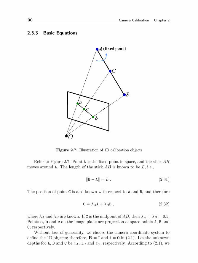
2.5.3 Basic Equations
Figure 2.7. Illustration of 1D calibration objects
Refer to Figure 2.7. Point A is the fixed point in space, and the stick ABmoves around A. The length of the stick AB is known to be L, i.e.,
‖B− A‖ = L . (2.31)
The position of point C is also known with respect to A and B, and therefore
C = λAA + λBB , (2.32)
where λA and λB are known. If C is the midpoint of AB, then λA = λB = 0.5.Points a, b and c on the image plane are projection of space points A, B andC, respectively.
Without loss of generality, we choose the camera coordinate system todefine the 1D objects; therefore, R = I and t = 0 in (2.1). Let the unknowndepths for A, B and C be zA, zB and zC , respectively. According to (2.1), we

Section 2.5. Solving Camera Calibration With 1D Objects 31
have
A = zAA−1a (2.33)
B = zBA−1b (2.34)
C = zCA−1c . (2.35)
Substituting them into (2.32) yields
zC c = zAλAa + zBλBb (2.36)
after eliminating A−1 from both sides. By performing cross-product on bothsides of the above equation with c, we have
zAλA(a× c) + zBλB(b× c) = 0 .
In turn, we obtain
zB = −zA λA(a× c) · (b× c)
λB(b× c) · (b× c). (2.37)
From (2.31), we have
‖A−1(zBb− zAa)‖ = L .
Substituting zB by (2.37) gives
zA‖A−1(a +λA(a× c) · (b× c)
λB(b× c) · (b× c)b)‖ = L .
This is equivalent toz2AhTA−TA−1h = L2 (2.38)
with
h = a +λA(a× c) · (b× c)
λB(b× c) · (b× c)b . (2.39)
Equation (2.38) contains the unknown intrinsic parameters A and the un-known depth, zA, of the fixed point A. It is the basic constraint for cameracalibration with 1D objects. Vector h, given by (2.39), can be computed fromimage points and known λA and λB. Since the total number of unknownsis 6, we need at least six observations of the 1D object for calibration. Notethat A−TA actually describes the image of the absolute conic [20].
32 Camera Calibration Chapter 2
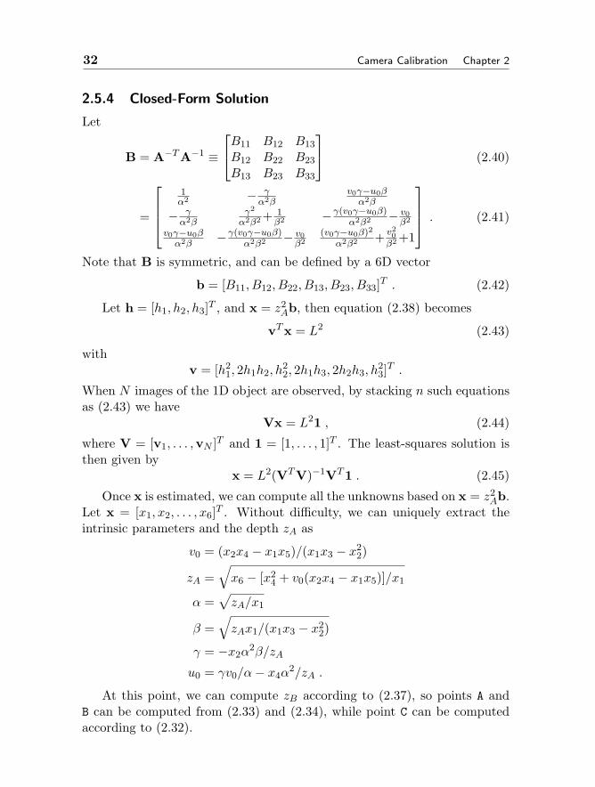
2.5.4 Closed-Form Solution
Let
B = A−TA−1 ≡B11 B12 B13B12 B22 B23B13 B23 B33
(2.40)
=
1α2 − γ
α2βv0γ−u0βα2β
− γα2β
γ2
α2β2 + 1β2 −γ(v0γ−u0β)
α2β2 − v0β2
v0γ−u0βα2β
−γ(v0γ−u0β)α2β2 − v0
β2(v0γ−u0β)2
α2β2 + v20β2 +1
. (2.41)
Note that B is symmetric, and can be defined by a 6D vector
b = [B11, B12, B22, B13, B23, B33]T . (2.42)
Let h = [h1, h2, h3]T , and x = z2Ab, then equation (2.38) becomes
vTx = L2 (2.43)
withv = [h2
1, 2h1h2, h22, 2h1h3, 2h2h3, h
23]T .
When N images of the 1D object are observed, by stacking n such equationsas (2.43) we have
Vx = L21 , (2.44)
where V = [v1, . . . ,vN ]T and 1 = [1, . . . , 1]T . The least-squares solution isthen given by
x = L2(VTV)−1VT1 . (2.45)
Once x is estimated, we can compute all the unknowns based on x = z2Ab.
Let x = [x1, x2, . . . , x6]T . Without difficulty, we can uniquely extract theintrinsic parameters and the depth zA as
v0 = (x2x4 − x1x5)/(x1x3 − x22)
zA =√x6 − [x2
4 + v0(x2x4 − x1x5)]/x1
α =√zA/x1
β =√zAx1/(x1x3 − x2
2)
γ = −x2α2β/zA
u0 = γv0/α− x4α2/zA .
At this point, we can compute zB according to (2.37), so points A andB can be computed from (2.33) and (2.34), while point C can be computedaccording to (2.32).
Section 2.5. Solving Camera Calibration With 1D Objects 33
2.5.5 Nonlinear Optimization
The above solution is obtained through minimizing an algebraic distancewhich is not physically meaningful. We can refine it through maximumlikelihood inference.
We are given N images of the 1D calibration object and there are 3points on the object. Point A is fixed, and points B and C moves around A.Assume that the image points are corrupted by independent and identicallydistributed noise. The maximum likelihood estimate can be obtained byminimizing the following functional:
N∑i=1
(‖ai − φ(A, A)‖2 + ‖bi − φ(A, Bi)‖2 + ‖ci − φ(A, Ci)‖2), (2.46)
where φ(A, M) (M ∈ A, Bi, Ci) is the projection of point M onto the image,according to equations (2.33) to (2.35). More precisely, φ(A, M) = 1
zMAM,
where zM is the z-component of M.The unknowns to be estimated are:
– 5 camera intrinsic parameters α, β, γ, u0 and v0 that define matrix A;
– 3 parameters for the coordinates of the fixed point A;
– 2N additional parameters to define points Bi and Ci at each instant(see below for more details).
Therefore, we have in total 8 + 2N unknowns. Regarding the parameteri-zation for B and C, we use the spherical coordinates φ and θ to define thedirection of the 1D calibration object, and point B is then given by
B = A + L
sin θ cosφsin θ sinφ
cos θ
where L is the known distance between A and B. In turn, point C is computedaccording to (2.32). We therefore only need 2 additional parameters for eachobservation.
Minimizing (2.46) is a nonlinear minimization problem, which is solvedwith the Levenberg-Marquardt Algorithm as implemented in Minpack [23].It requires an initial guess of A, A, Bi, Ci|i = 1..N which can be obtainedusing the technique described in the last subsection.
34 Camera Calibration Chapter 2
2.5.6 Estimating the fixed point
In the above discussion, we assumed that the image coordinates, a, of thefixed point A are known. We now describe how to estimate a by consideringwhether the fixed point A is visible in the image or not.
Invisible fixed point. The fixed point does not need to be visible in the image.And the camera calibration technique becomes more versatile without thevisibility requirement. In that case, we can for example hang a string ofsmall balls from the ceiling, and calibrate multiple cameras in the room byswinging the string. The fixed point can be estimated by intersecting linesfrom different images as described below.
Each observation of the 1D object defines an image line. An image linecan be represented by a 3D vector l = [l1, l2, l3]T , defined up to a scale factorsuch as a point m = [u, v]T on the line satisfies lT m = 0. In the sequel, wealso use (n, q) to denote line l, where n = [l1, l2]T and q = l3. To removethe scale ambiguity, we normalize l such that ‖l‖ = 1. Furthermore, each lis associated with an uncertainty measure represented by a 3× 3 covariancematrix Λ.
GivenN images of the 1D object, we haveN lines: (li,Λi)|i = 1, . . . , N.Let the fixed point be a in the image. Obviously, if there is no noise, wehave lTi a = 0, or nTi a + qi = 0. Therefore, we can estimate a by minimizing
F =N∑i=1
wi‖lTi a‖2 =N∑i=1
wi‖nTi a + qi‖2 =N∑i=1
wi(aTninTi a + 2qinTi a + q2i )
(2.47)where wi is a weighting factor (see below). By setting the derivative of Fwith respect to a to 0, we obtain the solution, which is given by
a = −( N∑i=1
wininTi)−1( N∑
i=1
wiqini).
The optimal weighting factor wi in (2.47) is the inverse of the variance of lTi a,which is wi = 1/(aTΛia). Note that the weight wi involves the unknown a.To overcome this difficulty, we can approximate wi by 1/ trace(Λi) for thefirst iteration, and by re-computing wi with the previously estimated a inthe subsequent iterations. Usually two or three iterations are enough.
Visible fixed point. Since the fixed point is visible, we have N observations:ai|i = 1, . . . , N. We can therefore estimate a by minimizing
∑Ni=1 ‖a−ai‖2,
assuming that the image points are detected with the same accuracy. Thesolution is simply a = (
∑Ni=1 ai)/N .

Section 2.5. Solving Camera Calibration With 1D Objects 35
The above estimation does not make use of the fact that the fixed pointis also the intersection of the N observed lines of the 1D object. Therefore,a better technique to estimate a is to minimize the following function:
F =N∑i=1
[(a−ai)TV−1
i (a−ai)+wi‖lTi a‖2]
=N∑i=1
[(a−ai)TV−1
i (a−ai)+wi‖nTi a+qi‖2]
(2.48)where Vi is the covariance matrix of the detected point ai. The derivativeof the above function with respect to a is given by
∂F∂a
= 2N∑i=1
[V−1i (a− ai) + wininTi a + wiqini
].
Setting it to 0 yields
a =( N∑i=1
(V−1i + wininTi )
)−1( N∑i=1
(V−1i ai − wiqini)
).
If more than three points are visible in each image, the known cross ratioprovides an additional constraint in determining the fixed point.
For an accessible description of uncertainty manipulation, the reader isreferred to [45, Chapter 2].
2.5.7 Experimental Results
The proposed algorithm has been tested on both computer simulated dataand real data.
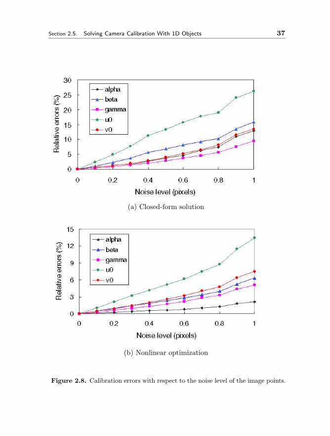
Computer Simulations
The simulated camera has the following property: α = 1000, β = 1000,γ = 0, u0 = 320, and v0 = 240. The image resolution is 640×480. A stick of70 cm is simulated with the fixed point A at [0, 35, 150]T . The other endpointof the stick is B, and C is located at the half way between A and B. We havegenerated 100 random orientations of the stick by sampling θ in [π/6, 5π/6]and φ in [π, 2π] according to uniform distribution. Points A, B, and C arethen projected onto the image.
Gaussian noise with 0 mean and σ standard deviation is added to theprojected image points a, b and c. The estimated camera parameters arecompared with the ground truth, and we measure their relative errors withrespect to the focal length α. Note that we measure the relative errors in
36 Camera Calibration Chapter 2
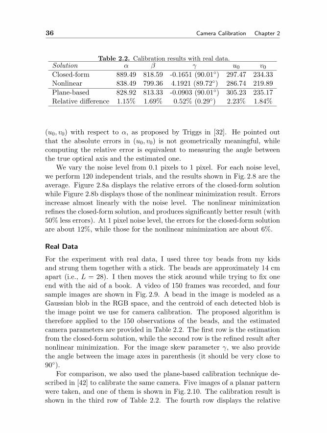
Table 2.2. Calibration results with real data.Solution α β γ u0 v0Closed-form 889.49 818.59 -0.1651 (90.01) 297.47 234.33Nonlinear 838.49 799.36 4.1921 (89.72) 286.74 219.89Plane-based 828.92 813.33 -0.0903 (90.01) 305.23 235.17Relative difference 1.15% 1.69% 0.52% (0.29) 2.23% 1.84%
(u0, v0) with respect to α, as proposed by Triggs in [32]. He pointed outthat the absolute errors in (u0, v0) is not geometrically meaningful, whilecomputing the relative error is equivalent to measuring the angle betweenthe true optical axis and the estimated one.
We vary the noise level from 0.1 pixels to 1 pixel. For each noise level,we perform 120 independent trials, and the results shown in Fig. 2.8 are theaverage. Figure 2.8a displays the relative errors of the closed-form solutionwhile Figure 2.8b displays those of the nonlinear minimization result. Errorsincrease almost linearly with the noise level. The nonlinear minimizationrefines the closed-form solution, and produces significantly better result (with50% less errors). At 1 pixel noise level, the errors for the closed-form solutionare about 12%, while those for the nonlinear minimization are about 6%.
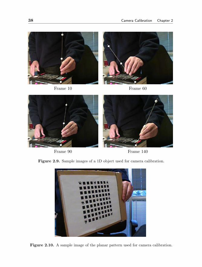
Real Data
For the experiment with real data, I used three toy beads from my kidsand strung them together with a stick. The beads are approximately 14 cmapart (i.e., L = 28). I then moves the stick around while trying to fix oneend with the aid of a book. A video of 150 frames was recorded, and foursample images are shown in Fig. 2.9. A bead in the image is modeled as aGaussian blob in the RGB space, and the centroid of each detected blob isthe image point we use for camera calibration. The proposed algorithm istherefore applied to the 150 observations of the beads, and the estimatedcamera parameters are provided in Table 2.2. The first row is the estimationfrom the closed-form solution, while the second row is the refined result afternonlinear minimization. For the image skew parameter γ, we also providethe angle between the image axes in parenthesis (it should be very close to90).
For comparison, we also used the plane-based calibration technique de-scribed in [42] to calibrate the same camera. Five images of a planar patternwere taken, and one of them is shown in Fig. 2.10. The calibration result isshown in the third row of Table 2.2. The fourth row displays the relative
Section 2.5. Solving Camera Calibration With 1D Objects 37
(a) Closed-form solution
(b) Nonlinear optimization
Figure 2.8. Calibration errors with respect to the noise level of the image points.
38 Camera Calibration Chapter 2
Frame 10 Frame 60
Frame 90 Frame 140
Figure 2.9. Sample images of a 1D object used for camera calibration.
Figure 2.10. A sample image of the planar pattern used for camera calibration.
Section 2.6. Self Calibration 39
difference between the plane-based result and the nonlinear solution with re-spect to the focal length (we use 828.92). As we can observe, the differenceis about 2%.
There are several sources contributing to this difference. Besides ob-viously the image noise and imprecision of the extracted data points, onesource is our current rudimentary experimental setup:
– The supposed-to-be fixed point was not fixed. It slipped around on thesurface.
– The positioning of the beads was done with a ruler using eye inspection.
Considering all the factors, the proposed algorithm is very encouraging.
2.6 Self-Calibration
Self-calibration is also called auto-calibration. Techniques in this categorydo not require any particular calibration object. They can be considered as0D approach because only image point correspondences are required. Justby moving a camera in a static scene, the rigidity of the scene provides ingeneral two constraints [22, 21, 20] on the cameras’ internal parameters fromone camera displacement by using image information alone. Absolute conic,described in Section 2.2.2, is an essential concept in understanding theseconstraints. Therefore, if images are taken by the same camera with fixedinternal parameters, correspondences between three images are sufficient torecover both the internal and external parameters which allow us to recon-struct 3-D structure up to a similarity [20, 17]. Although no calibrationobjects are necessary, a large number of parameters need to be estimated,resulting in a much harder mathematical problem.
We do not plan to go further into details of this approach because tworecent books [15, 7] provide an excellent recount of those techniques.
2.7 Conclusion
In this chapter, we have reviewed several camera calibration techniques. Wehave classified them into four categories, depending whether they use 3Dapparatus, 2D objects (planes), 1D objects, or just the surrounding scenes(self-calibration). Recommendations on choosing which technique were givenin the introduction section.
The techniques described so far are mostly focused on a single-cameracalibration. We touched a little bit on stereo calibration in Section 2.4.9.

40 Camera Calibration Chapter 2
Camera calibration is still an active research area because more and moreapplications use cameras. In [2], spheres are used to calibrate one or morecameras, which can be considered as a 2D approach since only the surfaceproperty is used. In [5], a technique is described to calibrate a camera net-work consisting of an omni-camera and a number of perspective cameras. In[24], a technique is proposed to calibrate a projector-screen-camera system.
2.8 Appendix: Estimating Homography Between the ModelPlane and its Image
There are many ways to estimate the homography between the model planeand its image. Here, we present a technique based on maximum likelihoodcriterion. Let Mi and mi be the model and image points, respectively. Ideally,they should satisfy (2.18). In practice, they don’t because of noise in theextracted image points. Let’s assume that mi is corrupted by Gaussian noisewith mean 0 and covariance matrix Λmi . Then, the maximum likelihoodestimation of H is obtained by minimizing the following functional∑
i
(mi − mi)TΛ−1mi
(mi − mi) ,
where mi =1
hT3 Mi
[hT1 MihT2 Mi
]with hi, the ith row of H.
In practice, we simply assume Λmi = σ2I for all i. This is reasonable if pointsare extracted independently with the same procedure. In this case, the aboveproblem becomes a nonlinear least-squares one, i.e., minH
∑i ‖mi − mi‖2.
The nonlinear minimization is conducted with the Levenberg-Marquardt Al-gorithm as implemented in Minpack [23]. This requires an initial guess,which can be obtained as follows.
Let x = [hT1 , hT2 , h
T3 ]T . Then equation (2.18) can be rewritten as[
MT 0T −uMT0T MT −vMT
]x = 0 .
When we are given n points, we have n above equations, which can be writtenin matrix equation as Lx = 0, where L is a 2n×9 matrix. As x is defined upto a scale factor, the solution is well known to be the right singular vector ofL associated with the smallest singular value (or equivalently, the eigenvectorof LTL associated with the smallest eigenvalue). In L, some elements areconstant 1, some are in pixels, some are in world coordinates, and some aremultiplication of both. This makes L poorly conditioned numerically. Muchbetter results can be obtained by performing a simple data normalizationprior to running the above procedure.
Bibliography 41
Bibliography
[1] Y.I. Abdel-Aziz and H.M. Karara. Direct linear transformation into objectspace coordinates in close-range photogrammetry. In Proceedings of the Sym-posium on Close-Range Photogrammetry, University of Illinois at Urbana-Champaign, Urbana, Illinois, pages 1–18, January 1971.
[2] M. Agrawal and L. Davis. Camera calibration using spheres: A semi-definiteprogramming approach. In Proceedings of the 9th International Conference onComputer Vision, pages 782–789, Nice, France, October 2003. IEEE ComputerSociety Press.
[3] D. C. Brown. Close-range camera calibration. Photogrammetric Engineering,37(8):855–866, 1971.
[4] B. Caprile and V. Torre. Using Vanishing Points for Camera Calibration. TheInternational Journal of Computer Vision, 4(2):127–140, March 1990.
[5] X. Chen, J. Yang, and A. Waibel. Calibration of a hybrid camera network.In Proceedings of the 9th International Conference on Computer Vision, pages150–155, Nice, France, October 2003. IEEE Computer Society Press.
[6] W. Faig. Calibration of close-range photogrammetry systems: Mathematicalformulation. Photogrammetric Engineering and Remote Sensing, 41(12):1479–1486, 1975.
[7] O. Faugeras and Q.-T. Luong. The Geometry of Multiple Images. The MITPress, 2001. With contributions from T. Papadopoulo.
[8] O. Faugeras. Three-Dimensional Computer Vision: a Geometric Viewpoint.MIT Press, 1993.
[9] O. Faugeras, T. Luong, and S. Maybank. Camera self-calibration: theory andexperiments. In G. Sandini, editor, Proc 2nd ECCV, volume 588 of LectureNotes in Computer Science, pages 321–334, Santa Margherita Ligure, Italy,May 1992. Springer-Verlag.
[10] O. Faugeras and G. Toscani. The calibration problem for stereo. In Proceedingsof the IEEE Conference on Computer Vision and Pattern Recognition, pages15–20, Miami Beach, FL, June 1986. IEEE.
[11] S. Ganapathy. Decomposition of transformation matrices for robot vision. Pat-tern Recognition Letters, 2:401–412, December 1984.
[12] D. Gennery. Stereo-camera calibration. In Proceedings of the 10th Image Un-derstanding Workshop, pages 101–108, 1979.
[13] G.H. Golub and C.F. van Loan. Matrix Computations. The John HopkinsUniversity Press, Baltimore, Maryland, 3 edition, 1996.
[14] P. Gurdjos, A. Crouzil, and R. Payrissat. Another way of looking at plane-basedcalibration: the centre circle constraint. In Proceedings of the 7th EuropeanConference on Computer Vision, volume IV, pages 252–266, Copenhagen, May2002.
[15] R. Hartley and A. Zisserman. Multiple View Geometry in Computer Vision.Cambridge University Press, 2000.
[16] R. Hartley. Self-calibration from multiple views with a rotating camera. In J-O. Eklundh, editor, Proceedings of the 3rd European Conference on ComputerVision, volume 800-801 of Lecture Notes in Computer Science, pages 471–478,Stockholm, Sweden, May 1994. Springer-Verlag.
42 Camera Calibration Chapter 2
[17] R. Hartley. An algorithm for self calibration from several views. In Proceedingsof the IEEE Conference on Computer Vision and Pattern Recognition, pages908–912, Seattle, WA, June 1994. IEEE.
[18] J. Heikkila and O. Silven. A four-step camera calibration procedure with im-plicit image correction. In Proceedings of the IEEE Conference on ComputerVision and Pattern Recognition, pages 1106–1112, San Juan, Puerto Rico, June1997. IEEE Computer Society.
[19] D. Liebowitz and A. Zisserman. Metric rectification for perspective images ofplanes. In Proceedings of the IEEE Conference on Computer Vision and Pat-tern Recognition, pages 482–488, Santa Barbara, California, June 1998. IEEEComputer Society.
[20] Q.-T. Luong and O.D. Faugeras. Self-calibration of a moving camera frompoint correspondences and fundamental matrices. The International Journal ofComputer Vision, 22(3):261–289, 1997.
[21] Q.-T. Luong. Matrice Fondamentale et Calibration Visuelle surl’Environnement-Vers une plus grande autonomie des systemes robotiques.PhD thesis, Universite de Paris-Sud, Centre d’Orsay, December 1992.
[22] S. J. Maybank and O. D. Faugeras. A theory of self-calibration of a movingcamera. The International Journal of Computer Vision, 8(2):123–152, August1992.
[23] J.J. More. The levenberg-marquardt algorithm, implementation and theory. InG. A. Watson, editor, Numerical Analysis, Lecture Notes in Mathematics 630.Springer-Verlag, 1977.
[24] T. Okatani and K. Deguchi. Autocalibration of projector-screen-camera sys-tem: Theory and algorithm for screen-to-camera homography estimation. InProceedings of the 9th International Conference on Computer Vision, pages774–781, Nice, France, October 2003. IEEE Computer Society Press.
[25] L. Robert. Camera calibration without feature extraction. Computer Vision,Graphics, and Image Processing, 63(2):314–325, March 1995. also INRIA Tech-nical Report 2204.
[26] J.G. Semple and G.T. Kneebone. Algebraic Projective Geometry. Oxford:Clarendon Press, 1952. Reprinted 1979.
[27] S.W. Shih, Y.P. Hung, and W.S. Lin. Accurate linear technique for cameracalibration considering lens distortion by solving an eigenvalue problem. OpticalEngineering, 32(1):138–149, 1993.
[28] I. Shimizu, Z. Zhang, S. Akamatsu, and K. Deguchi. Head pose determina-tion from one image using a generic model. In Proceedings of the IEEE ThirdInternational Conference on Automatic Face and Gesture Recognition, pages100–105, Nara, Japan, April 1998.
[29] C. C. Slama, editor. Manual of Photogrammetry. American Society of Pho-togrammetry, fourth edition, 1980.
[30] G. Stein. Accurate internal camera calibration using rotation, with analysis ofsources of error. In Proc. Fifth International Conference on Computer Vision,pages 230–236, Cambridge, Massachusetts, June 1995.
Bibliography 43
[31] P. Sturm and S. Maybank. On plane-based camera calibration: A generalalgorithm, singularities, applications. In Proceedings of the IEEE Conferenceon Computer Vision and Pattern Recognition, pages 432–437, Fort Collins,Colorado, June 1999. IEEE Computer Society Press.
[32] B. Triggs. Autocalibration from planar scenes. In Proceedings of the 5th Euro-pean Conference on Computer Vision, pages 89–105, Freiburg, Germany, June1998.
[33] R. Y. Tsai. A versatile camera calibration technique for high-accuracy 3D ma-chine vision metrology using off-the-shelf tv cameras and lenses. IEEE Journalof Robotics and Automation, 3(4):323–344, August 1987.
[34] T. Ueshiba and F. Tomita. Plane-based calibration algorithm for multi-camerasystems via factorization of homography matrices. In Proceedings of the 9thInternational Conference on Computer Vision, pages 966–973, Nice, France,October 2003. IEEE Computer Society Press.
[35] G.Q. Wei and S.D. Ma. A complete two-plane camera calibration methodand experimental comparisons. In Proc. Fourth International Conference onComputer Vision, pages 439–446, Berlin, May 1993.
[36] G.Q. Wei and S.D. Ma. Implicit and explicit camera calibration: Theory andexperiments. IEEE Transactions on Pattern Analysis and Machine Intelligence,16(5):469–480, 1994.
[37] J. Weng, P. Cohen, and M. Herniou. Camera calibration with distortion modelsand accuracy evaluation. IEEE Transactions on Pattern Analysis and MachineIntelligence, 14(10):965–980, October 1992.
[38] R. Willson. Modeling and Calibration of Automated Zoom Lenses. PhD thesis,Department of Electrical and Computer Engineering, Carnegie Mellon Univer-sity, 1994.
[39] R. Yang and Z. Zhang. Eye gaze correction with stereovision for video tele-conferencing. In Proceedings of the 7th European Conference on ComputerVision, volume II, pages 479–494, Copenhagen, May 2002. Also available asTechnical Report MSR-TR-01-119.
[40] R. Yang and Z. Zhang. Model-based head pose tracking with stereovision.In Proc. Fifth IEEE International Conference on Automatic Face and GestureRecognition (FG2002), pages 255–260, Washington, DC, May 2002. Also avail-able as Technical Report MSR-TR-01-102.
[41] Z. Zhang. A flexible new technique for camera calibration. Technical ReportMSR-TR-98-71, Microsoft Research, December 1998. Available together withthe software at http://research.microsoft.com/˜zhang/Calib/.
[42] Z. Zhang. A flexible new technique for camera calibration. IEEE Transactionson Pattern Analysis and Machine Intelligence, 22(11):1330–1334, 2000.
[43] Z. Zhang. Camera calibration with one-dimensional objects. Technical ReportMSR-TR-2001-120, Microsoft Research, December 2001.
[44] Z. Zhang. Camera calibration with one-dimensional objects. In Proc. Euro-pean Conference on Computer Vision (ECCV’02), volume IV, pages 161–174,Copenhagen, Denmark, May 2002.
[45] Z. Zhang and O.D. Faugeras. 3D Dynamic Scene Analysis: A Stereo BasedApproach. Springer, Berlin, Heidelberg, 1992.

Chapter 3
MULTIPLE VIEWGEOMETRY
Anders Heyden
and Marc Pollefeys
3.1 Introduction
There exist intricate geometric relations between multiple views of a 3Dscene. These relations are related to the camera motion and calibration aswell as to the scene structure. In this chapter we introduce these conceptsand discuss how they can be applied to recover 3D models from images.
In Section 3.2 a rather thorough description of projective geometry isgiven. Section 3.3 gives a short introduction to tensor calculus and Sec-tion 3.4 describes in detail the camera model used. In Section 3.5 a modernapproach to multiple view geometry is presented and in Section 3.6 simplestructure and motion algorithms are presented. In Section 3.7 more ad-vanced algorithms are presented that are suited for automatic processing onreal image data. Section 3.8 discusses the possibility of calibrating the cam-era from images. Section 3.9 describes how the depth can be computed formost image pixels and Section 3.10 presents how the results of the previoussections can be combined to yield 3D models, render novel views or combinereal and virtual elements in video.
45
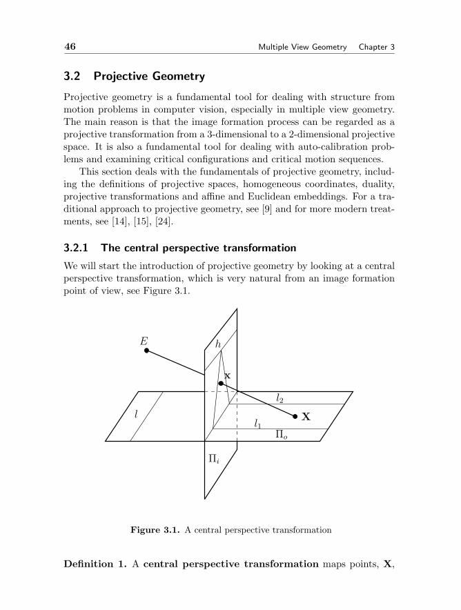
46 Multiple View Geometry Chapter 3
3.2 Projective Geometry
Projective geometry is a fundamental tool for dealing with structure frommotion problems in computer vision, especially in multiple view geometry.The main reason is that the image formation process can be regarded as aprojective transformation from a 3-dimensional to a 2-dimensional projectivespace. It is also a fundamental tool for dealing with auto-calibration prob-lems and examining critical configurations and critical motion sequences.
This section deals with the fundamentals of projective geometry, includ-ing the definitions of projective spaces, homogeneous coordinates, duality,projective transformations and affine and Euclidean embeddings. For a tra-ditional approach to projective geometry, see [9] and for more modern treat-ments, see [14], [15], [24].
3.2.1 The central perspective transformation
We will start the introduction of projective geometry by looking at a centralperspective transformation, which is very natural from an image formationpoint of view, see Figure 3.1.
x
Πi
E
Πo
X
h
l
l2
l1
Figure 3.1. A central perspective transformation
Definition 1. A central perspective transformation maps points, X,
Section 3.2. Projective Geometry 47
on the object plane, Πo, to points on the image plane Πi, by intersecting theline through E, called the centre, and X with Πi.
We can immediately see the following properties of the planar perspectivetransformation:
– All points on Πo maps to points on Πi except for points on l, where lis defined as the intersection of Πo with the plane incident with E andparallel with Πi.
– All points on Πi are images of points on Πo except for points on h,called the horizon, where h is defined as the intersection of Πi withthe plane incident with E and parallel with Πo.
– Lines in Πo are mapped to lines in Πi.– The images of parallel lines intersects in a point on the horizon, see
e.g. l1 and l2 in Figure 3.1.– In the limit where the point E moves infinitely far away, the planar
perspective transformation turns into a parallel projection.Identify the planes Πo and Πi with R
2, with a standard cartesian coordinatesystem Oe1e2 in Πo and Πi respectively. The central perspective transfor-mation is nearly a bijective transformation between Πo and Πi, i.e. from R
2
to R2. The problem is the lines l ∈ Πo and h ∈ Πi. If we remove these lines
we obtain a bijective transformation between R2 \ l and R
2 \ h, but this isnot the path that we will follow. Instead, we extend each R
2 with an extraline defined as the images of points on h and points that maps to l, in thenatural way, i.e. maintaining continuity. Thus by adding one artificial lineto each plane, it is possible to make the central perspective transformationbijective from (R2 + an extra line) to (R2 + an extra line). These extra linescorrespond naturally to directions in the other plane, e.g. the images of thelines l1 and l2 intersects in a point on h corresponding to the direction of l1and l2. The intersection point on h can be viewed as the limit of images of apoint on l1 moving infinitely far away. Inspired by this observation we makethe following definition:
Definition 2. Consider the set L of all lines parallel to a given line l in R2
and assign a point to each such set, pideal, called an ideal point or pointat infinity, cf. Figure 3.2.
3.2.2 Projective spaces
We are now ready to make a preliminary definition of the two-dimensionalprojective space, i.e. the projective plane.
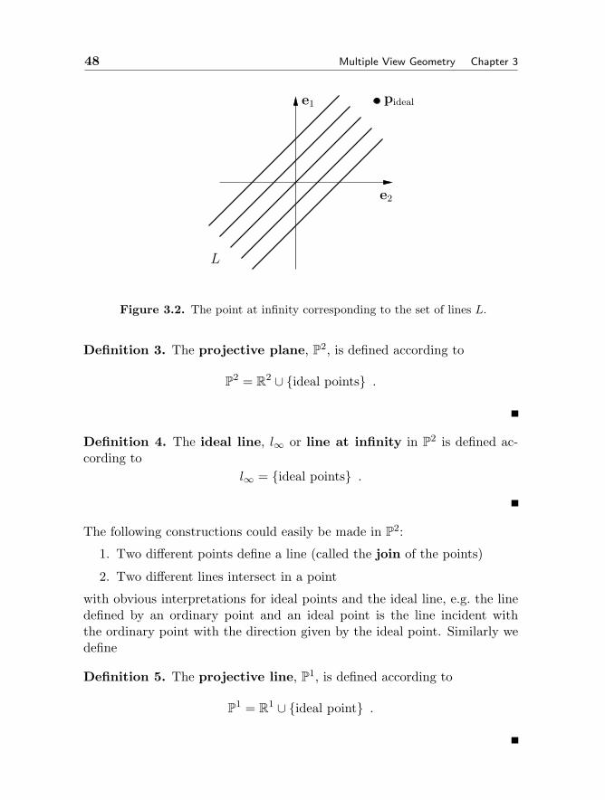
48 Multiple View Geometry Chapter 3
pideal
L
e1
e2
Figure 3.2. The point at infinity corresponding to the set of lines L.
Definition 3. The projective plane, P2, is defined according to
P2 = R
2 ∪ ideal points .
Definition 4. The ideal line, l∞ or line at infinity in P2 is defined ac-
cording tol∞ = ideal points .
The following constructions could easily be made in P2:
1. Two different points define a line (called the join of the points)
2. Two different lines intersect in a point
with obvious interpretations for ideal points and the ideal line, e.g. the linedefined by an ordinary point and an ideal point is the line incident withthe ordinary point with the direction given by the ideal point. Similarly wedefine
Definition 5. The projective line, P1, is defined according to
P1 = R
1 ∪ ideal point .

Section 3.2. Projective Geometry 49
Observe that the projective line only contains one ideal point, which couldbe regarded as the point at infinity.
In order to define three-dimensional projective space, P3, we start with
R3 and assign an ideal point to each set of parallel lines, i.e. to each direction.
Definition 6. The projective space, P3, is defined according to
P3 = R
3 ∪ ideal points .
Observe that the ideal points in P3 constitutes a two-dimensional manifold,
which motivates the following definition.
Definition 7. The ideal points in P3 builds up a plane, called the ideal
plane or plane at infinity, also containing ideal lines.
The plane at infinity contains lines, again called lines at infinity. Every setof parallel planes in R
3 defines an ideal line and all ideal lines builds up theideal plane. A lot of geometrical constructions can be made in P
3, e.g.
1. Two different points define a line (called the join of the two points)
2. Three different points define a plane (called the join of the three points)
3. Two different planes intersect in a line
4. Three different planes intersect in a point
3.2.3 Homogeneous coordinates
It is often advantageous to introduce coordinates in the projective spaces, socalled analytic projective geometry. Introduce a cartesian coordinate system,Oexey in R
2 and define the line l : y = 1, see Figure 3.3. We make thefollowing simple observations:
Lemma 1. The vectors (p1, p2) and (q1, q2) determines the same line throughthe origin iff
(p1, p2) = λ(q1, q2), λ = 0 .
Proposition 1. Every line, lp = (p1, p2)t, t ∈ R, through the origin, exceptfor the x-axis, intersect the line l in one point, p.
We can now make the following definitions:
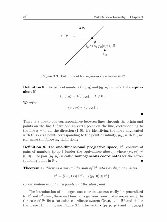
50 Multiple View Geometry Chapter 3
lp : (p1.p2)t, t ∈ R
ex
ey
p
l : y = 1
Figure 3.3. Definition of homogeneous coordinates in P1.
Definition 8. The pairs of numbers (p1, p2) and (q1, q2) are said to be equiv-alent if
(p1, p2) = λ(q1, q2), λ = 0 .
We write(p1, p2) ∼ (q1, q2) .
There is a one-to-one correspondence between lines through the origin andpoints on the line l if we add an extra point on the line, corresponding tothe line x = 0, i.e. the direction (1, 0). By identifying the line l augmentedwith this extra point, corresponding to the point at infinity, p∞, with P
1, wecan make the following definitions:
Definition 9. The one-dimensional projective space, P1, consists of
pairs of numbers (p1, p2) (under the equivalence above), where (p1, p2) =(0, 0). The pair (p1, p2) is called homogeneous coordinates for the corre-sponding point in P
1.
Theorem 1. There is a natural division of P1 into two disjoint subsets
P1 = (p1, 1) ∈ P
1 ∪ (p1, 0) ∈ P1 ,
corresponding to ordinary points and the ideal point.
The introduction of homogeneous coordinates can easily be generalizedto P
2 and P3 using three and four homogeneous coordinates respectively. In
the case of P2 fix a cartesian coordinate system Oexeyez in R
3 and definethe plane Π : z = 1, see Figure 3.4. The vectors (p1, p2, p3) and (q1, q2, q3)
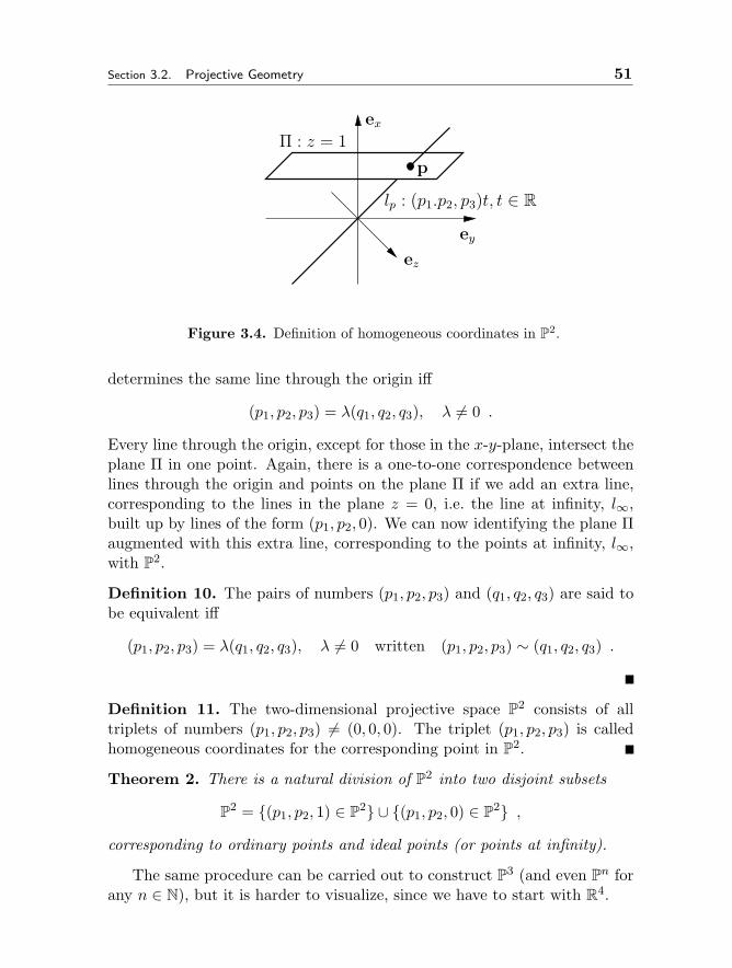
Section 3.2. Projective Geometry 51
p
ex
ey
lp : (p1.p2, p3)t, t ∈ R
Π : z = 1
ez
Figure 3.4. Definition of homogeneous coordinates in P2.
determines the same line through the origin iff
(p1, p2, p3) = λ(q1, q2, q3), λ = 0 .
Every line through the origin, except for those in the x-y-plane, intersect theplane Π in one point. Again, there is a one-to-one correspondence betweenlines through the origin and points on the plane Π if we add an extra line,corresponding to the lines in the plane z = 0, i.e. the line at infinity, l∞,built up by lines of the form (p1, p2, 0). We can now identifying the plane Πaugmented with this extra line, corresponding to the points at infinity, l∞,with P
2.
Definition 10. The pairs of numbers (p1, p2, p3) and (q1, q2, q3) are said tobe equivalent iff
(p1, p2, p3) = λ(q1, q2, q3), λ = 0 written (p1, p2, p3) ∼ (q1, q2, q3) .
Definition 11. The two-dimensional projective space P2 consists of all
triplets of numbers (p1, p2, p3) = (0, 0, 0). The triplet (p1, p2, p3) is calledhomogeneous coordinates for the corresponding point in P
2.
Theorem 2. There is a natural division of P2 into two disjoint subsets
P2 = (p1, p2, 1) ∈ P
2 ∪ (p1, p2, 0) ∈ P2 ,
corresponding to ordinary points and ideal points (or points at infinity).
The same procedure can be carried out to construct P3 (and even P
n forany n ∈ N), but it is harder to visualize, since we have to start with R
4.
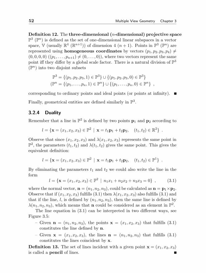
52 Multiple View Geometry Chapter 3
Definition 12. The three-dimensional (n-dimensional) projective spaceP
3 (Pn) is defined as the set of one-dimensional linear subspaces in a vectorspace, V (usually R
4 (Rn+1)) of dimension 4 (n + 1). Points in P3 (Pn) are
represented using homogeneous coordinates by vectors (p1, p2, p3, p4) =(0, 0, 0, 0) ((p1, . . . , pn+1) = (0, . . . , 0)), where two vectors represent the samepoint iff they differ by a global scale factor. There is a natural division of P
3
(Pn) into two disjoint subsets
P3 = (p1, p2, p3, 1) ∈ P
3 ∪ (p1, p2, p3, 0) ∈ P3
(Pn = (p1, . . . , pn, 1) ∈ Pn ∪ (p1, . . . , pn, 0) ∈ P
n ,corresponding to ordinary points and ideal points (or points at infinity).
Finally, geometrical entities are defined similarly in P3.
3.2.4 Duality
Remember that a line in P2 is defined by two points p1 and p2 according to
l = x = (x1, x2, x3) ∈ P2 | x = t1p1 + t2p2, (t1, t2) ∈ R
2 .Observe that since (x1, x2, x3) and λ(x1, x2, x3) represents the same point inP
2, the parameters (t1, t2) and λ(t1, t2) gives the same point. This gives theequivalent definition:
l = x = (x1, x2, x3) ∈ P2 | x = t1p1 + t2p2, (t1, t2) ∈ P
1 .By eliminating the parameters t1 and t2 we could also write the line in theform
l = x = (x1, x2, x3) ∈ P2 | n1x1 + n2x2 + n3x3 = 0 , (3.1)
where the normal vector, n = (n1, n2, n3), could be calculated as n = p1×p2.Observe that if (x1, x2, x3) fulfills (3.1) then λ(x1, x2, x3) also fulfills (3.1) andthat if the line, l, is defined by (n1, n2, n3), then the same line is defined byλ(n1, n2, n3), which means that n could be considered as an element in P
2.The line equation in (3.1) can be interpreted in two different ways, see
Figure 3.5:– Given n = (n1, n2, n3), the points x = (x1, x2, x3) that fulfills (3.1)
constitutes the line defined by n.– Given x = (x1, x2, x3), the lines n = (n1, n2, n3) that fulfills (3.1)
constitutes the lines coincident by x.Definition 13. The set of lines incident with a given point x = (x1, x2, x3)is called a pencil of lines.

Section 3.2. Projective Geometry 53
In this way there is a one-to-one correspondence between points and lines inP
2 given byx = (a, b, c) ↔ n = (a, b, c) ,
as illustrated in Figure 3.5.
e1
e2 e2
e1
Figure 3.5. Duality of points and lines in P2.
Similarly, there exists a duality between points and planes in P3. A plane
π in P3 consists of the points x = (x1, x2, x3, x4) that fulfill the equation
π = x = (x1, x2, x3, x4) ∈ P3 | n1x1 + n2x2 + n3x3 + n4x4 = 0 , (3.2)
where n = (n1, n2, n3, n4) defines the plane. From (3.2) a similar argumentleads to a duality between planes and points in P
3. The following theoremis fundamental in projective geometry:
Theorem 3. Given a statement valid in a projective space. Then the dualto that statement is also valid, where the dual is obtained by interchangingentities with their duals, intersection with join etc.
For instance, a line in P3 could be defined as the join of two points. Thus
the dual to a line is the intersection of two planes, which again is a line, i.e.the dual to a line in P
3 is a line. We say that lines are self-dual. A line inP
3 defined as the join of two points, p1 and p2, as in
l = x = (x1, x2, x3, x4) ∈ P3 | x = t1p1 + t2p2, (t1, t2) ∈ P
1
is said to be given in parametric form and (t1, t2) can be regarded ashomogeneous coordinates on the line. A line in P
3 defined as the intersection
54 Multiple View Geometry Chapter 3
of two planes, π and µ, consists of the common points to the pencil of planesin
l : sπ + tµ | (s, t) ∈ P1
is said to be given in intersection form.
Definition 14. A conic, c, in P2 is defined as
c = x = (x1, x2, x3) ∈ P2 | xTCx = 0 , (3.3)
where C denotes 3 × 3 matrix. If C is non-singular the conic is said to beproper, otherwise it is said to be degenerate.
The dual to a general curve in P2 (P3) is defined as the set of tangent lines
(tangent planes) to the curve.
Theorem 4. The dual, c∗, to a conic c : xTCx is the set of lines
l = (l1, l2, l3) ∈ P2 | lTC ′l = 0 ,
where C ′ = C−1.
3.2.5 Projective transformations
The central perspective transformation in Figure 3.1 is an example of aprojective transformation. The general definition is as follows:
Definition 15. A projective transformation from p ∈ Pn to p′ ∈ P
m isdefined as a linear transformation in homogeneous coordinates, i.e.
x′ ∼ Hx , (3.4)
where x and x′ denote homogeneous coordinates for p and p′ respectivelyand H denote a (m+ 1)× (n+ 1)-matrix of full rank.
All projective transformations form a group, denoted GP . For example aprojective transformation from x ∈ P
2 to y ∈ P2 is given byy1
y2y3
∼ Hx1x2x3
,
where H denote a non-singular 3× 3-matrix. Such a projective transforma-tion from P
2 to P2 is usually called a homography.
It is possible to embed an affine space in the projective space, by a simpleconstruction:
Section 3.2. Projective Geometry 55
Definition 16. The subspaces
Ani = (x1, x2, . . . , xn+1) ∈ Pn | xi = 0
of Pn, are called affine pieces of P
n. The plane Hi : xi = 0 is called theplane at infinity, corresponding to the affine piece Ani . Usually, i = n+ 1is used and called the standard affine piece and in this case the plane atinfinity is denoted H∞.
We can now identify points in An with points, x, in Ani ⊂ P
n, by
Pn (x1, x2, . . . , xn, xn+1) ∼ (y1, y2, . . . , yn, 1) ≡ (y1, y2, . . . , yn) ∈ A
n .
There is even an affine structure in this affine piece, given by the followingproposition:
Proposition 2. The subgroup, H, of projective transformations, GP , thatpreserves the plane at infinity consists exactly of the projective transforma-tions of the form (3.4), with
H =[An×n bn×101×n 1
],
where the indices denote the sizes of the matrices.
We can now identify the affine transformations in A with the subgroup H:
A x → Ax + b ∈ A ,
which gives the affine structure in Ani ⊂ Pn.
Definition 17. When a plane at infinity has been chosen, two lines are saidto be parallel if they intersect at a point at the plane at infinity.
We may even go one step further and define a Euclidean structure in Pn.
Definition 18. The (singular, complex) conic, Ω, in Pn defined by
x21 + x2
1 + . . .+ x2n = 0 and xn+1 = 0
is called the absolute conic.
Observe that the absolute conic is located at the plane at infinity, it containsonly complex points and it is singular.
56 Multiple View Geometry Chapter 3
Lemma 2. The dual to the absolute conic, denoted Ω′, is given by the set ofplanes
Ω′ = Π = (Π1,Π2, . . .Πn+1) | Π21 + . . .+ Π2
n = 0 .
In matrix form Ω′ can be written as ΠTC ′Π = 0 with
C ′ =[In×n 0n×101×n 0
].
Proposition 3. The subgroup, K, of projective transformations, GP , thatpreserves the absolute conic consists exactly of the projective transformationsof the form (3.4), with
H =[cRn×n tn×101×n 1
],
where 0 = c ∈ R and R denote an orthogonal matrix, i.e. RRT = RTR = I.
Observe that the corresponding transformation in the affine space A =An+1n can be written as
A x → cRx + t ∈ A ,
which is a similarity transformation. This means that we have a Euclideanstructure (to be precise a similarity structure) in P
n given by the absoluteconic.
3.3 Tensor Calculus
Tensor calculus is a natural tool to use, when the objects at study are ex-pressed in a specific coordinate system, but have physical properties thatare independent on the chosen coordinate system. Another advantage isthat it gives a simple and compact notation and the rules for tensor algebramakes it easy to remember even quite complex formulas. For a more detailedtreatment see [58] and for an engineering approach see [42].
In this chapter a simple definition of a tensor and the basic rules formanipulating tensors are given. We start with a straight-forward definition:
Definition 19. An affine tensor is an object in a linear space, V, thatconsists of a collection of numbers, that are related to a specific choice ofcoordinate system in V, indexed by one or several indices;
Ai1,i2,··· ,inj1,j2,··· ,jm .
Section 3.3. Tensor Calculus 57
Furthermore, this collection of numbers transforms in a pre-defined way whena change of coordinate system in V is made, see Definition 20. The numberof indices (n + m) is called the degree of the tensor. The indices maytake any value from 1 to the dimension of V. The upper indices are calledcontravariant indices and the lower indices are called covariant indices.
There are some simple conventions, that have to be remembered:– The index rule: When an index appears in a formula, the formula is
valid for every value of the index, i.e. ai = 0⇒ a1 = 0, a2 = 0, . . .– The summation convention: When an index appears twice in a formula,
it is implicitly assumed that a summation takes place over that index,i.e. aibi =
∑i=1,dim V aib
i
– The compatibility rule: A repeated index must appear once as a sub-index and once as a super-index
– The maximum rule: An index can not be used more than twice in aterm
Definition 20. When the coordinate system in V is changed from e to eand the points with coordinates x are changed to x, according to
ej = Sijei ⇔ xi = Sijxj ,
then the affine tensor components change according to
uk = Sjkuj and vj = Sjkvk ,
for lower and upper indices respectively.
From this definition the terminology for indices can be motivated, sincethe covariant indices co-varies with the basis vectors and the contravariantindices contra-varies with the basis vectors. It turns out that a vector (e.g.the coordinates of a point) is a contravariant tensor of degree one and that aone-form (e.g. the coordinate of a vector defining a line in R
2 or a hyperplanein R
n) is a covariant tensor of degree one.
Definition 21. The second order tensor
δij =
1 i = j
0 i = j
is called the Kronecker delta. When dimV = 3, the third order tensor
εijk =
1 (i,j,k) an even permutation−1 (i,j,k) an odd permutation0 (i,j,k) has a repeated value
is called the Levi-Cevita epsilon.
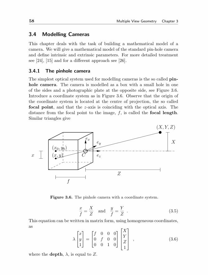
58 Multiple View Geometry Chapter 3
3.4 Modelling Cameras
This chapter deals with the task of building a mathematical model of acamera. We will give a mathematical model of the standard pin-hole cameraand define intrinsic and extrinsic parameters. For more detailed treatmentsee [24], [15] and for a different approach see [26].
3.4.1 The pinhole camera
The simplest optical system used for modelling cameras is the so called pin-hole camera. The camera is modelled as a box with a small hole in oneof the sides and a photographic plate at the opposite side, see Figure 3.6.Introduce a coordinate system as in Figure 3.6. Observe that the origin ofthe coordinate system is located at the centre of projection, the so calledfocal point, and that the z-axis is coinciding with the optical axis. Thedistance from the focal point to the image, f , is called the focal length.Similar triangles give
ex
C
ey
ez
Z
f
X
(X, Y, Z)
x (x, y)(x0, y0)
Figure 3.6. The pinhole camera with a coordinate system.
x
f=X
Zand
y
f=Y
Z. (3.5)
This equation can be written in matrix form, using homogeneous coordinates,as
λ
xy1
=
f 0 0 00 f 0 00 0 1 0
XYZ1
, (3.6)
where the depth, λ, is equal to Z.
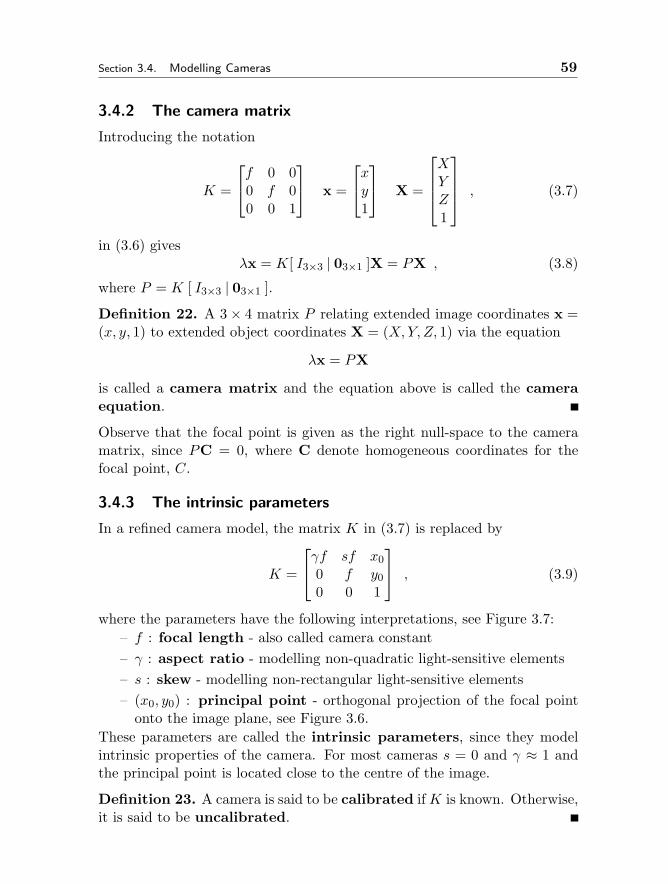
Section 3.4. Modelling Cameras 59
3.4.2 The camera matrix
Introducing the notation
K =
f 0 00 f 00 0 1
x =
xy1
X =
XYZ1
, (3.7)
in (3.6) givesλx = K[ I3×3 | 03×1 ]X = PX , (3.8)
where P = K [ I3×3 | 03×1 ].
Definition 22. A 3× 4 matrix P relating extended image coordinates x =(x, y, 1) to extended object coordinates X = (X,Y, Z, 1) via the equation
λx = PX
is called a camera matrix and the equation above is called the cameraequation.
Observe that the focal point is given as the right null-space to the cameramatrix, since PC = 0, where C denote homogeneous coordinates for thefocal point, C.
3.4.3 The intrinsic parameters
In a refined camera model, the matrix K in (3.7) is replaced by
K =
γf sf x00 f y00 0 1
, (3.9)
where the parameters have the following interpretations, see Figure 3.7:– f : focal length - also called camera constant– γ : aspect ratio - modelling non-quadratic light-sensitive elements– s : skew - modelling non-rectangular light-sensitive elements– (x0, y0) : principal point - orthogonal projection of the focal point
onto the image plane, see Figure 3.6.These parameters are called the intrinsic parameters, since they modelintrinsic properties of the camera. For most cameras s = 0 and γ ≈ 1 andthe principal point is located close to the centre of the image.
Definition 23. A camera is said to be calibrated ifK is known. Otherwise,it is said to be uncalibrated.
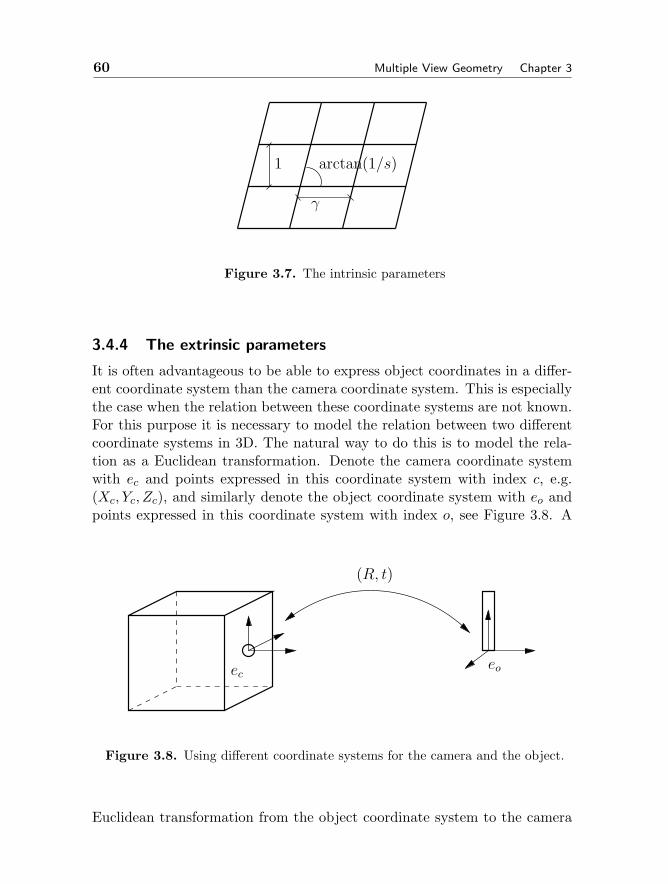
60 Multiple View Geometry Chapter 3
γ
1 arctan(1/s)
Figure 3.7. The intrinsic parameters
3.4.4 The extrinsic parameters
It is often advantageous to be able to express object coordinates in a differ-ent coordinate system than the camera coordinate system. This is especiallythe case when the relation between these coordinate systems are not known.For this purpose it is necessary to model the relation between two differentcoordinate systems in 3D. The natural way to do this is to model the rela-tion as a Euclidean transformation. Denote the camera coordinate systemwith ec and points expressed in this coordinate system with index c, e.g.(Xc, Yc, Zc), and similarly denote the object coordinate system with eo andpoints expressed in this coordinate system with index o, see Figure 3.8. A
(R, t)
eceo
Figure 3.8. Using different coordinate systems for the camera and the object.
Euclidean transformation from the object coordinate system to the camera

Section 3.4. Modelling Cameras 61
coordinate system can be written in homogeneous coordinates asXc
YcZc1
=[RT 00 1
] [I −t0 1
]Xo
YoZo1
=⇒ Xc =[RT −RT t0 1
]Xo , (3.10)
where R denote an orthogonal matrix and t a vector, encoding the rotationand translation in the rigid transformation. Observe that the focal point(0, 0, 0) in the c-system corresponds to the point t in the o-system. Inserting(3.10) in (3.8) taking into account that X in (3.8) is the same as Xc in (3.10),we obtain
λx = KRT [ I | − t ]Xo = PX , (3.11)
with P = KRT [ I | − t ]. Usually, it is assumed that object coordinates areexpressed in the object coordinate system and the index o in Xo is omitted.Observe that the focal point, Cf = t = (tx, ty, tz), is given from the rightnull-space to P according to
P
txtytz1
= KRT [ I | − t ]
txtytz1
= 0 .
Given a camera, described by the camera matrix P , this camera could alsobe described by the camera matrix µP , 0 = µ ∈ R, since these give the sameimage point for each object point. This means that the camera matrix isonly defined up to an unknown scale factor. Moreover, the camera matrix Pcan be regarded as a projective transformation from P
3 to P2, cf. (3.8) and
(3.4).Observe also that replacing t by µt and (X,Y, Z) with (µX, µY, µZ),
0 = µ ∈ R, gives the same image since
KRT [ I | − µt ]
µXµYµZ1
= µKRT [ I | − t ]
XYZ1
.
We refer to this ambiguity as the scale ambiguity.We can now calculate the number of parameters in the camera matrix,
P :
– K: 5 parameters (f , γ, s, x0, y0)
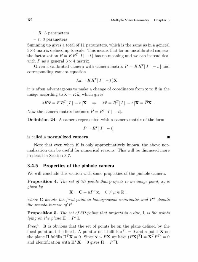
62 Multiple View Geometry Chapter 3
– R: 3 parameters– t: 3 parameters
Summing up gives a total of 11 parameters, which is the same as in a general3×4 matrix defined up to scale. This means that for an uncalibrated camera,the factorization P = KRT [ I | − t ] has no meaning and we can instead dealwith P as a general 3× 4 matrix.
Given a calibrated camera with camera matrix P = KRT [ I | − t ] andcorresponding camera equation
λx = KRT [ I | − t ]X ,
it is often advantageous to make a change of coordinates from x to x in theimage according to x = Kx, which gives
λKx = KRT [ I | − t ]X ⇒ λx = RT [ I | − t ]X = PX .
Now the camera matrix becomes P = RT [ I | − t].Definition 24. A camera represented with a camera matrix of the form
P = RT [ I | − t]is called a normalized camera.
Note that even when K is only approximatively known, the above nor-malization can be useful for numerical reasons. This will be discussed morein detail in Section 3.7.
3.4.5 Properties of the pinhole camera
We will conclude this section with some properties of the pinhole camera.
Proposition 4. The set of 3D-points that projects to an image point, x, isgiven by
X = C + µP+x, 0 = µ ∈ R ,
where C denote the focal point in homogeneous coordinates and P+ denotethe pseudo-inverse of P .
Proposition 5. The set of 3D-points that projects to a line, l, is the pointslying on the plane Π = P T l.
Proof: It is obvious that the set of points lie on the plane defined by thefocal point and the line l. A point x on l fulfills xT l = 0 and a point X onthe plane Π fulfills ΠTX = 0. Since x ∼ PX we have (PX)T l = XTP T l = 0and identification with ΠTX = 0 gives Π = P T l.
Section 3.5. Multiple View Geometry 63
Lemma 3. The projection of a quadric, XTCX = 0 (dually ΠTC ′Π = 0,C ′ = C−1), is an image conic, xT cx = 0 (dually lT c′l = 0, c′ = c−1), withc′ = PC ′P T .
Proof: Use the previous proposition.
Proposition 6. The image of the absolute conic is given by the conic xTωx =0 (dually lTω′l = 0), where ω′ = KKT .
Proof: The result follows from the previous lemma:
ω′ ∼ PΩ′P T ∼ KRT [I −t] [I 00 0
] [I−tT
]RKT = KRTRKT = KKT .
3.5 Multiple View Geometry
Multiple view geometry is the subject where relations between coordinatesof feature points in different views are studied. It is an important toolfor understanding the image formation process for several cameras and fordesigning reconstruction algorithms. For a more detailed treatment, see [27]or [24] and for a different approach see [26]. For the algebraic properties ofmultilinear constraints see [30].
3.5.1 The structure and motion problem
The following problem is central in computer vision:
Problem 1. structure and motion Given a sequence of images with corre-sponding feature points xij, taken by a perspective camera, i.e.
λijxij = PiXj , i = 1, . . . ,m, j = 1, . . . , n ,
determine the camera matrices, Pi, i.e. the motion, and the 3D-points,Xj, i.e. the structure, under different assumptions on the intrinsic and/orextrinsic parameters. This is called the structure and motion problem.
It turns out that there is a fundamental limitation on the solutions to thestructure and motion problem, when the intrinsic parameters are unknownand possibly varying, a so called un-calibrated image sequence.
Theorem 5. Given an un-calibrated image sequence with correspondingpoints, it is only possible to reconstruct the object up to an unknown pro-jective transformation.
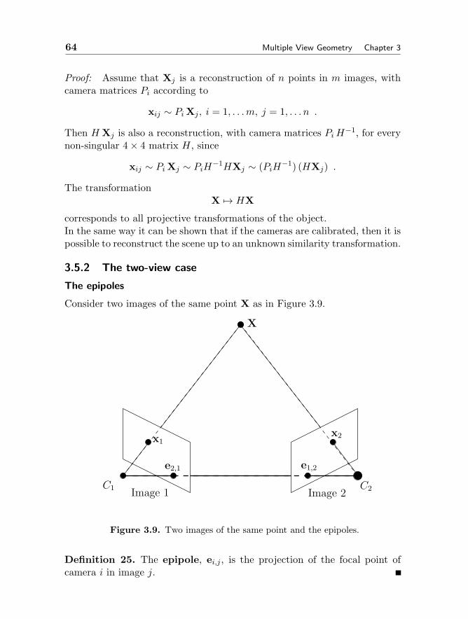
64 Multiple View Geometry Chapter 3
Proof: Assume that Xj is a reconstruction of n points in m images, withcamera matrices Pi according to
xij ∼ PiXj , i = 1, . . .m, j = 1, . . . n .
Then HXj is also a reconstruction, with camera matrices PiH−1, for everynon-singular 4× 4 matrix H, since
xij ∼ PiXj ∼ PiH−1HXj ∼ (PiH−1) (HXj) .
The transformationX → HX
corresponds to all projective transformations of the object.In the same way it can be shown that if the cameras are calibrated, then it ispossible to reconstruct the scene up to an unknown similarity transformation.
3.5.2 The two-view case
The epipoles
Consider two images of the same point X as in Figure 3.9.
C1
x1
e2,1
X
e1,2
x2
C2Image 2Image 1
Figure 3.9. Two images of the same point and the epipoles.
Definition 25. The epipole, ei,j , is the projection of the focal point ofcamera i in image j.
Section 3.5. Multiple View Geometry 65
Proposition 7. Let
P1 = [ A1 | b1 ] and P2 = [ A2 | b2 ] .
Then the epipole, e1,2 is given by
e1,2 = −A2A−11 b1 + b2 . (3.12)
Proof: The focal point of camera 1, C1, is given by
P1
[C11
]= [ A1 | b1 ]
[C11
]= A1C1 + b1 = 0 ,
i.e. C1 = −A−11 b1 and then the epipole is obtained from
P2
[C11
]= [ A2 | b2 ]
[C11
]= A2C1 + b2 = −A2A
−11 b1 + b2 .
It is convenient to use the notation A12 = A2A−11 . Assume that we have
calculated two camera matrices, representing the two-view geometry,
P1 = [ A1 | b1 ] and P2 = [ A2 | b2 ] .
According to Theorem 5 we can multiply these camera matrices with
H =[A−1
1 −A−11 b1
0 1
]from the right and obtain
P1 = P1H = [ I | 0 ] P2 = P2H = [ A2A−11 | b2 −A2A
−11 b1 ] .
Thus, we may always assume that the first camera matrix is [ I | 0 ]. Observethat P2 = [ A12 | e ], where e denotes the epipole in the second image.Observe also that we may multiply again with
H =[I 0vT 1
]without changing P1, but
HP2 = [ A12 + evT | e ] ,
i.e. the last column of the second camera matrix still represents the epipole.
Definition 26. A pair of camera matrices is said to be in canonical formif
P1 = [ I | 0 ] and P2 = [ A12 + evT | e ] , (3.13)
where v denote a three-parameter ambiguity.
66 Multiple View Geometry Chapter 3
The fundamental matrix
The fundamental matrix was originally discovered in the calibrated case in[38] and in the uncalibrated case in [13]. Consider a fixed point, X, in 2views:
λ1x1 = P1X = [ A1 | b1 ]X, λ2x2 = P2X = [ A2 | b2 ]X .
Use the first camera equation to solve for X, Y , Z
λ1x1 = P1X = [ A1 | b1 ]X = A1
XYZ
+ b1 ⇒XYZ
= A−11 (λ1x1 − b1)
and insert into the second one
λ2x2 = A2A−11 (λ1x1 − b1) + b2 = λ1A12x1 + (−A12b1 − b2) ,
i.e. x2, A12x1 and t = −A12b1 + b2 = e1,2 are linearly dependent. Observethat t = e1,2, i.e. the epipole in the second image. This condition can bewritten as xT1A
T12Tex2 = xT1 Fx2 = 0, with F = AT12Te, where Tx denote the
skew-symmetric matrix corresponding to the vector x, i.e. Tx(y) = x× y.Definition 27. The bilinear constraint
xT1 Fx2 = 0 (3.14)
is called the epipolar constraint and
F = AT12Te
is called the fundamental matrix.
Theorem 6. The epipole in the second image is obtain as the right nullspaceto the fundamental matrix and the epipole in the left image is obtained asthe left nullspace to the fundamental matrix.
Proof: Follows from Fe = AT12Tee = AT12(e× e) = 0. The statement aboutthe epipole in the left image follows from symmetry.
Corollary 1. The fundamental matrix is singular, i.e. detF = 0.
Given a point, x1, in the first image, the coordinates of the correspondingpoint in the second image fulfill
0 = xT1 Fx2 = (xT1 F )x2 = l(x1)Tx2 = 0 ,
where l(x1) denote the line represented by xT1 F .
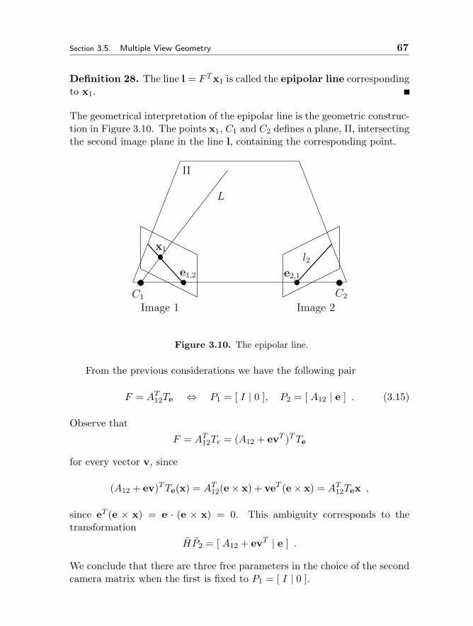
Section 3.5. Multiple View Geometry 67
Definition 28. The line l = F Tx1 is called the epipolar line correspondingto x1.
The geometrical interpretation of the epipolar line is the geometric construc-tion in Figure 3.10. The points x1, C1 and C2 defines a plane, Π, intersectingthe second image plane in the line l, containing the corresponding point.
e2,1
Image 1 Image 2
x1
C1 C2
e1,2
l2
Π
L
Figure 3.10. The epipolar line.
From the previous considerations we have the following pair
F = AT12Te ⇔ P1 = [ I | 0 ], P2 = [ A12 | e ] . (3.15)
Observe that
F = AT12Te = (A12 + evT )TTe
for every vector v, since
(A12 + ev)TTe(x) = AT12(e× x) + veT (e× x) = AT12Tex ,
since eT (e × x) = e · (e × x) = 0. This ambiguity corresponds to thetransformation
HP2 = [ A12 + evT | e ] .
We conclude that there are three free parameters in the choice of the secondcamera matrix when the first is fixed to P1 = [ I | 0 ].
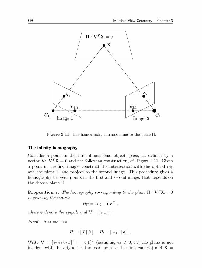
68 Multiple View Geometry Chapter 3
x1
e1,2
X
e2,1
x2
C2Image 2Image 1C1
Π : VTX = 0
Figure 3.11. The homography corresponding to the plane Π.
The infinity homography
Consider a plane in the three-dimensional object space, Π, defined by avector V: VTX = 0 and the following construction, cf. Figure 3.11. Givena point in the first image, construct the intersection with the optical rayand the plane Π and project to the second image. This procedure gives ahomography between points in the first and second image, that depends onthe chosen plane Π.
Proposition 8. The homography corresponding to the plane Π : VTX = 0is given by the matrix
HΠ = A12 − evT ,
where e denote the epipole and V = [v 1 ]T .
Proof: Assume that
P1 = [ I | 0 ], P2 = [ A12 | e ] .
Write V = [ v1 v2 v3 1 ]T = [v 1 ]T (assuming v4 = 0, i.e. the plane is notincident with the origin, i.e. the focal point of the first camera) and X =
Section 3.5. Multiple View Geometry 69
[X Y ZW ]T = [wW ]T , which gives
VTX = vTw +W , (3.16)
which implies that vTw = −W for points in the plane Π. The first cameraequation gives
x1 ∼ [ I | 0 ]X = w
and using (3.16) gives vTx1 = −W . Finally, the second camera matrix gives
x2 ∼ [ A12 | e ][
x1−vTx1
]= A12x1 − evTx1 = (A12 − evT )x1 .
Observe that when V = (0, 0, 0, 1), i.e. v = (0, 0, 0) the plane Π is the planeat infinity.
Definition 29. The homography
H∞ = HΠ∞ = A12
is called the homography corresponding to the plane at infinity orinfinity homography.
Note that the epipolar line through the point x2 in the second image can bewritten as x2 × e, implying
(x2 × e)THx1 = xT1HTTex2 = 0 ,
i.e. the epipolar constraint and we get
F = HTTe .
Proposition 9. There is a one to one correspondence between planes in 3D,homographies between two views and factorization of the fundamental matrixas F = HTTe.
Finally, we note that the matrix HTΠTeHΠ is skew symmetric, implying that
FHΠ +HTΠF
T = 0 . (3.17)

70 Multiple View Geometry Chapter 3
3.5.3 Multi-view constraints and tensors
Consider one object point, X, and its m images, xi, according to the cameraequations λixi = PiX, i = 1 . . .m. These equations can be written as
P1 x1 0 0 . . . 0P2 0 x2 0 . . . 0P3 0 0 x3 . . . 0...
......
.... . .
...Pm 0 0 0 . . . xm
︸ ︷︷ ︸
M
X−λ1−λ2−λ3
...−λm
=
000...0
. (3.18)
We immediately get the following proposition:
Proposition 10. The matrix, M , in (3.18) is rank deficient, i.e.
rankM < m+ 4 ,
which is referred to as the rank condition.
The rank condition implies that all (m+4)× (m+4) minors of M are equalto 0. These can be written using Laplace expansions as sums of productsof determinants of four rows taken from the first four columns of M and ofimage coordinates. There are 3 different categories of such minors dependingon the number of rows taken from each image, since one row has to be takenfrom each image and then the remaining 4 rows can be distributed freely.The three different types are:
1. Take the 2 remaining rows from one camera matrix and the 2 remainingrows from another camera matrix, gives 2-view constraints.
2. Take the 2 remaining rows from one camera matrix, 1 row from anotherand 1 row from a third camera matrix, gives 3-view constraints.
3. Take 1 row from each of four different camera matrices, gives 4-viewconstraints.
Observe that the minors of M can be factorized as products of the 2-, 3-or 4-view constraint and image coordinates in the other images. In order toget a notation that connects to the tensor notation we will use (x1, x2, x3)instead of (x, y, z) for homogeneous image coordinates. We will also denoterow number i of a camera matrix P by P i.
Section 3.5. Multiple View Geometry 71
The monofocal tensor
Before we proceed to the multi-view tensors we make the following observa-tion:
Proposition 11. The epipole in image 2 from camera 1, e = (e1, e2, e3) inhomogeneous coordinates, can be written as
ej = det
P 1
1P 2
1P 3
1P j2
. (3.19)
Proposition 12. The numbers ej constitutes a first order contravarianttensor, where the transformations of the tensor components are related toprojective transformations of the image coordinates.
Definition 30. The first order contravariant tensor, ej , is called the mono-focal tensor.
The bifocal tensor
Considering minors obtained by taking 3 rows from one image, and 3 rowsfrom another image:
det[P1 x1 0P2 0 x2
]= det
P 11 x1
1 0P 2
1 x21 0
P 31 x3
1 0P 1
2 0 x12
P 22 0 x2
2P 3
2 0 x32
= 0 ,
which gives a bilinear constraint:
3∑i,j=1
Fijxi1xj2 = Fijxi1x
j2 = 0 , (3.20)
where
Fij =3∑
i′,i′′,j′,j′′=1
εii′i′′εjj′j′′ det
P i
′1
P i′′
1
P j′
2
P j′′
2
.
The following proposition follows from (3.20).
72 Multiple View Geometry Chapter 3
Proposition 13. The numbers Fij constitutes a second order covariant ten-sor.
Here the transformations of the tensor components are related to projectivetransformations of the image coordinates.
Definition 31. The second order covariant tensor, Fij , is called the bifocaltensor and the bilinear constraint in (3.20) is called the bifocal constraint.
Observe that the indices tell us which row to exclude from the correspondingcamera matrix when forming the determinant. The geometric interpretationof the bifocal constraint is that corresponding view-lines in two images in-tersect in 3D, cf. Figure 3.9. The bifocal tensor can also be used to trans-fer a point to the corresponding epipolar line, cf. Figure 3.10, according tol2j = Fijxi1. This transfer can be extended to a homography between epipolarlines in the first view and epipolar lines in the second view according to
l1i = Fijεjj′j′′ l2j′ej
′′,
since εjj′
j′′ l2j′ej′′
gives the cross product between the epipole e and the line l2,which gives a point on the epipolar line.
The trifocal tensor
The trifocal tensor was originally discovered in the calibrated case in [60]and in the uncalibrated case in [55]. Considering minors obtained by taking3 rows from one image, 2 rows from another image and 2 rows from a thirdimage, e.g.
det
P 11 x1
1 0 0P 2
1 x21 0 0
P 31 x3
1 0 0P 1
2 0 x12 0
P 22 0 x2
2 0P 1
3 0 0 x13
P 33 0 0 x3
3
= 0 ,
gives a trilinear constraints:
3∑i,j,j′,k,k′=1
T jki xi1εjj′j′′xj′
2 εkk′k′′xk′
3 = 0 , (3.21)
Section 3.5. Multiple View Geometry 73
where
T jki =3∑
i′,i′′=1
εii′i′′ det
P i
′1
P i′′
1P j2P k3
. (3.22)
Note that there are in total 9 constraints indexed by j′′ and k′′ in (3.21).
Proposition 14. The numbers T jki constitutes a third order mixed tensor,that is covariant in i and contravariant in j and k.
Definition 32. The third order mixed tensor, T jki is called the trifocal ten-sor and the trilinear constraint in (3.21) is called the trifocal constraint.
Again the lower index tells us which row to exclude from the first cameramatrix and the upper indices tell us which rows to include from the secondand third camera matrices respectively and these indices becomes covariantand contravariant respectively. Observe that the order of the images areimportant, since the first image is treated differently. If the images are per-muted another set of coefficients are obtained. The geometric interpretationof the trifocal constraint is that the view-line in the first image and the planescorresponding to arbitrary lines coincident with the corresponding points inthe second and third images (together with the focal points) respectivelyintersect in 3D, cf. Figure 3.12. The following theorem is straightforward toprove.
Theorem 7. Given three corresponding lines, l1, l2 and l3 in three image,represented by the vectors (l11, l
12, l
13) etc. Then
l3k = T ijk l1i l2j . (3.23)
From this theorem it is possible to transfer the images of a line seen in twoimages to a third image, so called tensorial transfer. The geometricalinterpretation is that two corresponding lines defines two planes in 3D, thatintersect in a line, that can be projected onto the third image. There arealso other transfer equations, such as
xj2 = T jki xi1l3k and xk3 = T jki xj2l
3k ,
with obvious geometrical interpretations.

74 Multiple View Geometry Chapter 3
C3
x1
l3
Image 3
C1
Image 1
l2
Image 2C2
X
Figure 3.12. Geometrical interpretation of the trifocal constraint.
The quadrifocal tensor
The quadrifocal tensor was independently discovered in several papers, e.g.[64], [26]. Considering minors obtained by taking 2 rows from each one of 4different images gives a quadrilinear constraint:
3∑i,i′,j,j′,k,k′,l,l′=1
Qijklεii′i′′x1i′εjj′j′′x2
j′εkk′k′′x3k′εll′l′′x4
l′ = 0 , (3.24)
where
Qijkl = det
P i1P j2P k3P l4
.
Note that there are in total 81 constraints indexed by i′′, j′′, k′′ and l′′ in(3.24).
Proposition 15. The numbers Qijkl constitutes a fourth order contravarianttensor.
Section 3.6. Structure and Motion I 75
Definition 33. The fourth order contravariant tensor, Qijkl is called thequadrifocal tensor and the quadrilinear constraint in (3.24) is called thequadrifocal constraint.
Note that there are in total 81 constraints indexed by i′′, j′′, k′′ and l′′.Again, the upper indices tell us which rows to include from each cameramatrix respectively they become contravariant indices. The geometric inter-pretation of the quadrifocal constraint is that the four planes correspondingto arbitrary lines coincident with the corresponding points in the imagesintersect in 3D.
3.6 Structure and Motion I
We will now study the structure and motion problem in detail. Firstly, wewill solve the problem when the structure in known, so called resection, thenwhen the motion is known, so called intersection. Then we will present alinear algorithm to solve for both structure and motion using the multifocaltensors and finally a factorization algorithm will be presented. Again werefer the reader to [24] for a more detailed treatment.
3.6.1 Resection
Problem 2 (Resection). Assume that the structure is given, i.e. the objectpoints, Xj, j = 1, . . . n are given in some coordinate system. Calculate thecamera matrices Pi, i = 1, . . .m from the images, i.e. from xi,j.
The most simple solution to this problem is the classical DLT algorithmbased on the fact that the camera equations
λjxj = PXj , j = 1 . . . n
are linear in the unknown parameters, λj and P .
3.6.2 Intersection
Problem 3 (Intersection). Assume that the motion is given, i.e. the cam-era matrices, Pi, i = 1, . . .m are given in some coordinate system. Calculatethe structure Xj, j = 1, . . . n from the images, i.e. from xi,j.
Consider the image of X in camera 1 and 2λ1x1 = P1X,
λ2x2 = P2X,(3.25)
76 Multiple View Geometry Chapter 3
which can be written in matrix form as (cf. (3.18))
[P1 x1 0P2 0 x2
] X−λ1−λ2
= 0 , (3.26)
which again is linear in the unknowns, λi and X. This linear method can ofcourse be extended to an arbitrary number of images.
3.6.3 Linear estimation of tensors
We are now able to solve the structure and motion problem given in Prob-lem 1. The general scheme is as follows
1. Estimate the components of a multiview tensor linearly from imagecorrespondences
2. Extract the camera matrices from the tensor components3. Reconstruct the object using intersection, i.e. (3.26)
The eight-point algorithm
Each point correspondence gives one linear constraint on the components ofthe bifocal tensor according to the bifocal constraint:
Fijxi1xj2 = 0 .
Each pair of corresponding points gives a linear homogeneous constraint onthe nine tensor components Fij . Thus given at least eight correspondingpoints we can solve linearly (e.g. by SVD) for the tensor components. Afterthe bifocal tensor (fundamental matrix) has been calculated it has to befactorized as F = A12T
Te , which can be done by first solving for e using
Fe = 0 (i.e. finding the right nullspace to F ) and then for A12, by solvinglinear system of equations. One solution is
A12 =
0 0 0F13 F23 F33−F12 −F22 −F32
,
which can be seen from the definition of the tensor components. In the caseof noisy data it might happen that detF = 0 and the right nullspace doesnot exist. One solution is to solve Fe = 0 in least squares sense using SVD.Another possibility is to project F to the closest rank-2 matrix, again usingSVD. Then the camera matrices can be calculated from (3.26) and finallyusing intersection, (3.25) to calculate the structure.
Section 3.6. Structure and Motion I 77
The seven-point algorithm
A similar algorithm can be constructed for the case of corresponding pointsin three images.
Proposition 16. The trifocal constraint in (3.21) contains 4 linearly inde-pendent constraints in the tensor components T jki .
Corollary 2. At least 7 corresponding points in three views are needed inorder to estimate the 27 homogeneous components of the trifocal tensor.
The main difference to the eight-point algorithm is that it is not obvious howto extract the camera matrices from the trifocal tensor components. Startwith the transfer equation
xj2 = T jki xi1l3k ,
which can be seen as a homography between the first two images, by fixinga line in the third image. The homography is the one corresponding to theplane Π defined by the focal point of the third camera and the fixed line inthe third camera. Thus we know from (3.17) that the fundamental matrixbetween image 1 and image 2 obeys
FT ·J· + (T ·J
· )TF T = 0 ,
where T ·J· denotes the matrix obtained by fixing the index J . Since this is alinear constraint on the components of the fundamental matrix, it can easilybe extracted from the trifocal tensor. Then the camera matrices P1 and P2could be calculated and finally, the entries in the third camera matrix P3 canbe recovered linearly from the definition of the tensor components in (3.22),cf. [27].
An advantage of using three views is that lines could be used to constrainthe geometry, using (3.23), giving two linearly independent constraints foreach corresponding line.
The six-point algorithm
Again a similar algorithm can be constructed for the case of correspondingpoints in four images.
Proposition 17. The quadrifocal constraint in (3.24) contains 16 linearlyindependent constraints in the tensor components Qijkl.
From this proposition it seems as 5 corresponding points would be suffi-cient to calculate the 81 homogeneous components of the quadrifocal tensor.However, the following proposition says that this is not possible

78 Multiple View Geometry Chapter 3
Proposition 18. The quadrifocal constraint in (3.24) for 2 correspondingpoints contains 31 linearly independent constraints in the tensor componentsQijkl.
Corollary 3. At least 6 corresponding points in three views are needed inorder to estimate the 81 homogeneous components of the quadrifocal tensor.
Since one independent constraint is lost for each pair of corresponding pointsin four images, we get 6 · 16− ( 6
2 ) = 81 linearly independent constraints.Again, it is not obvious how to extract the camera matrices from the
trifocal tensor components. First, a trifocal tensor has to be extracted andthen a fundamental matrix and finally the camera matrices. It is outsidethe scope of this work to give the details for this, see [27]. Also in thiscase corresponding lines can be used by looking at transfer equations for thequadrifocal tensor.
3.6.4 Factorization
A disadvantage with using multiview tensors to solve the structure and mo-tion problem is that when many images ( 4) are available, the informationin all images can not be used with equal weight. An alternative is to use aso called factorization method, see [59].
Write the camera equations
λi,jxi,j = PiXj , i = 1, . . . ,m, j = 1, . . . , n
for a fixed image i in matrix form as
XiΛi = PiX , (3.27)
where
Xi =[xTi,1 xTi,2 . . . xTi,n
], X =
[XT
1 XT2 . . . XT
n
],
Λi = diag(λi,1, λi,2, . . . , λi,n) .
The camera matrix equations for all images can now be written as
X = PX , (3.28)
where
X =
X1Λ1X2Λ2
...XmΛm
, P =
P1P2...P3
.
Section 3.6. Structure and Motion I 79
Observe that X only contains image measurements apart from the unknowndepths.
Proposition 19.
rank X ≤ 4
This follows from (3.28) since X is a product of a 3m×4 and a 4×n matrix.Assume that the depths, i.e. Λi are known, corresponding to affine cameras,we may use the following simple factorization algorithm:
1. Build up the matrix X from image measurements.
2. Factorize X = UΣV T using SVD.
3. Extract P = the first four columns of UΣ and X = the first four rowsof V T .
In the perspective case this algorithm can be extended to the so called iter-ative factorization algorithm:
1. Set λi,j = 1.
2. Build up the matrix X from image measurements and the current es-timate of λi,j .
3. Factorize X = UΣV T using SVD.
4. Extract P = the first four columns of UΣ and X = the first four rowsof V T .
5. Use the current estimate of P and X to improve the estimate of thedepths from the camera equations XiΛi = PiX.
6. If the error (re-projection errors or σ5) is too large goto 2.
Definition 34. The fifth singular value, σ5 in the SVD above is called theproximity measure and is a measure of the accuracy of the reconstruction.
Theorem 8. The algorithm above minimizes the proximity measure.
Figure 3.13 shows an example of a reconstruction using the iterative factor-ization method applied on four images of a toy block scene. Observe thatthe proximity measure decreases quite fast and the algorithm converges inabout 20 steps.
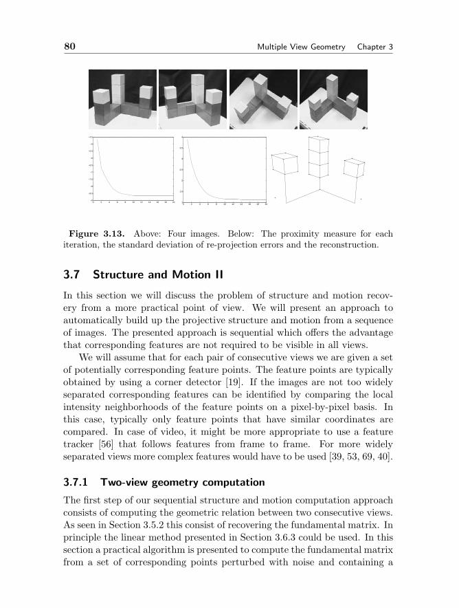
80 Multiple View Geometry Chapter 3
0 2 4 6 8 10 12 14 16 18 201
1.5
2
2.5
3
3.5
4
0 2 4 6 8 10 12 14 16 18 20−9
−8.5
−8
−7.5
−7
−6.5
−6
−5.5
−5
−4.5
Figure 3.13. Above: Four images. Below: The proximity measure for eachiteration, the standard deviation of re-projection errors and the reconstruction.
3.7 Structure and Motion II
In this section we will discuss the problem of structure and motion recov-ery from a more practical point of view. We will present an approach toautomatically build up the projective structure and motion from a sequenceof images. The presented approach is sequential which offers the advantagethat corresponding features are not required to be visible in all views.
We will assume that for each pair of consecutive views we are given a setof potentially corresponding feature points. The feature points are typicallyobtained by using a corner detector [19]. If the images are not too widelyseparated corresponding features can be identified by comparing the localintensity neighborhoods of the feature points on a pixel-by-pixel basis. Inthis case, typically only feature points that have similar coordinates arecompared. In case of video, it might be more appropriate to use a featuretracker [56] that follows features from frame to frame. For more widelyseparated views more complex features would have to be used [39, 53, 69, 40].
3.7.1 Two-view geometry computation
The first step of our sequential structure and motion computation approachconsists of computing the geometric relation between two consecutive views.As seen in Section 3.5.2 this consist of recovering the fundamental matrix. Inprinciple the linear method presented in Section 3.6.3 could be used. In thissection a practical algorithm is presented to compute the fundamental matrixfrom a set of corresponding points perturbed with noise and containing a
Section 3.7. Structure and Motion II 81
significant proportion of outliers.
Linear algorithms
Before presenting the complete robust algorithm we will first revisit the linearalgorithm. Given a number of corresponding points (3.14) can be used tocompute F . This equation can be rewritten in the following form:[
x1x2 y1x2 x2 x1y2 y1y2 y2 x1 y1 1]f = 0 (3.29)
with x1 = [x1 y1 1],x2 = [x2 y2 1] and f a vector containing the elementsof the fundamental matrix. As discussed before, stacking 8 or more of theseequations allows for a linear solution. Even for 7 corresponding points theone parameter family of solutions obtained by solving the linear equationscan be restricted to 1 or 3 solutions by enforcing the cubic rank-2 con-straint det (F1 + λF2) = 0. Note also that, as pointed out by Hartley [22],it is important to normalize the image coordinates before solving the linearequations. Otherwise the columns of (3.29) would differ by several ordersof magnitude and the error would be concentrated on the coefficients cor-responding to the smaller columns. This normalization can be achieved bytransforming the image center to the origin and scaling the images so thatthe coordinates have a standard deviation of unity.
Non-linear algorithms
The result of the linear equations can be refined by minimizing the followingcriterion [70]:
C(F ) =∑(
d(x2, Fx1)2 + d(x1, Fx2)2
)(3.30)
with d(., .) representing the Euclidean distance in the image. This criterioncan be minimized through a Levenberg-Marquard algorithm [50]. An evenbetter approach consists of computing the maximum-likelyhood estimation(for Gaussian noise) by minimizing the following criterion:
C(F, x1, x2) =∑(
d(x1,x1)2 + d(x2,x2)2)
with x2 F x1 = 0 (3.31)
Although in this case the minimization has to be carried out over a muchlarger set of variables, this can be achieved efficiently by taking advantageof the sparsity of the problem.
82 Multiple View Geometry Chapter 3
Robust algorithm
To compute the fundamental matrix from a set of matches that were auto-matically obtained from a pair of real images, it is important to explicitlydeal with outliers. If the set of matches is contaminated with even a smallset of outliers, the result of the above methods can become unusable. This istypical for all types of least-squares approaches (even non-linear ones). Theproblem is that the quadratic penalty allows for a single outlier that is veryfar away from the true solution to completely bias the final result.
An approach that can be used to cope with this problem is the RANSACalgorithm that was proposed by Fischler and Bolles [17]. A minimal subsetof the data, in this case 7 point correspondences, is randomly selected fromthe set of potential correspondences and the solution obtained from it isused to segment the remainder of the dataset in inliers and outliers. Ifthe initial subset contains no outliers, most of the correct correspondenceswill support the solution. However, if one or more outliers are contained inthe initial subset, it is highly improbable that the computed solution willfind a lot of support among the remainder of the potential correspondences,yielding a low “inlier” ratio. This procedure is repeated until a satisfyingsolution is obtained. This is typically defined as a probability in excess of95% that a good subsample was selected. The expression for this probabilityis Γ = 1− (1−ρp)m with ρ the fraction of inliers, p the number of features ineach sample, 7 in this case, and m the number of trials (see Rousseeuw [51]).
Two-view geometry computation
The different algorithms described above can be combined to yield a practicalalgorithm to compute the two-view geometry from real images:
1. Compute initial set of potential correspondences (and set ρmax =0,m = 0)
2. While (1− (1− ρ7max)
m) < 95% do(a) Randomly select a minimal sample (7 pairs of corresponding points)
(b) Compute the solution(s) for F (yielding 1 or 3 solutions)(c) Determine percentage of inliers ρ (for all solutions)(d) Increment m, update ρmax if ρmax < ρ
3. Refine F based on all inliers4. Look for additional matches along epipolar lines5. Refine F based on all correct matches (preferably using (3.31))
Section 3.7. Structure and Motion II 83
3.7.2 Structure and motion recovery
Once the epipolar geometry has been computed between all consecutiveviews, the next step consists of reconstructing the structure and motionfor the whole sequence. To the contrary of the factorization approach ofSection 3.6.4, here a sequential approach is presented. First the structureand motion is initialized for two views and then gradually extended towardsthe whole sequence. Finally, the solution is refined through a global mini-mization over all the unknown parameters.
Initializing the structure and motion
Initial motion computation Two images of the sequence are used to deter-mine a reference frame. The world frame is aligned with the first camera.The second camera is chosen so that the epipolar geometry corresponds tothe retrieved fundamental matrix F :
P1 = [ I3×3 | 03 ]P2 = [ TeF + ev | σe ]
(3.32)
Eq. (3.32) is not completely determined by the epipolar geometry (i.e. F ande), but has 4 more degrees of freedom (i.e. v and σ). The vector v determinesthe position of the reference plane (i.e. the plane at infinity in an affine ormetric frame) and σ determines the global scale of the reconstruction. Thelocation of the reference plane shouldn’t make any difference if the algorithmis projectively invariant. To achieve this it is important to use homogeneousrepresentations for all 3D entities and to only use image measurements forminimizations. The value for the parameter σ has no importance and canbe fixed to one.
Initial structure computation Once two projection matrices have been fullydetermined the matches can be reconstructed through triangulation. Dueto noise the lines of sight will not intersect perfectly. In the projective casethe minimizations should be carried out in the images and not in projective3D space. Therefore, the distance between the reprojected 3D point and theimage points should be minimized:
d(x1, P1X)2 + d(x2, P2X)2 (3.33)
It was noted by Hartley and Sturm [23] that the only important choice is toselect in which epipolar plane the point is reconstructed. Once this choice ismade it is trivial to select the optimal point from the plane. Since a bundleof epipolar planes only has one parameter, the dimension of the problem

84 Multiple View Geometry Chapter 3
is reduced from three to one. Minimizing the following equation is thusequivalent to minimizing equation (3.33).
d(x1, l1(λ))2 + d(x2, l2(λ))2 (3.34)
with l1(λ) and l2(λ) the epipolar lines obtained in function of the parameterλ describing the bundle of epipolar planes. It turns out (see [23]) that thisequation is a polynomial of degree 6 in λ. The global minimum of equa-tion (3.34) can thus easily be computed directly. In both images the pointson the epipolar line l1(λ) and l2(λ) closest to the points x1 resp. x2 are se-lected. Since these points are in epipolar correspondence their lines of sightintersect exactly in a 3D point. In the case where (3.31) had been mini-mized to obtain the fundamental matrix F the procedure described here isunnecessary and the pairs (x1, x2) can be reconstructed directly.
Updating the structure and motion
The previous section dealt with obtaining an initial reconstruction from twoviews. This section discusses how to add a view to an existing reconstruction.First the pose of the camera is determined, then the structure is updatedbased on the added view and finally new points are initialized.
projective pose estimation For every additional view the pose towards thepre-existing reconstruction is determined. This is illustrated in Figure 3.14.It is assumed that the epipolar geometry has been computed between viewi− 1 and i. The matches which correspond to already reconstructed pointsare used to infer correspondences between 2D and 3D. Based on these theprojection matrix Pi is computed using a robust procedure similar to theone laid out for computing the fundamental matrix. In this case a minimalsample of 6 matches is needed to compute Pi. A point is considered an inlierif there exists a 3D point that projects sufficiently close to all associatedimage points. This requires to refine the initial solution of X based on allobservations, including the last. Because this is computationally expensive(remember that this has to be done for each generated hypothesis), it isadvised to use a modified version of RANSAC that cancels the verificationof unpromising hypothesis [5]. Once Pi has been determined the projectionof already reconstructed points can be predicted, so that some additionalmatches can be obtained. This means that the search space is graduallyreduced from the full image to the epipolar line to the predicted projectionof the point.
This procedure only relates the image to the previous image. In fact it isimplicitly assumed that once a point gets out of sight, it will not come back.
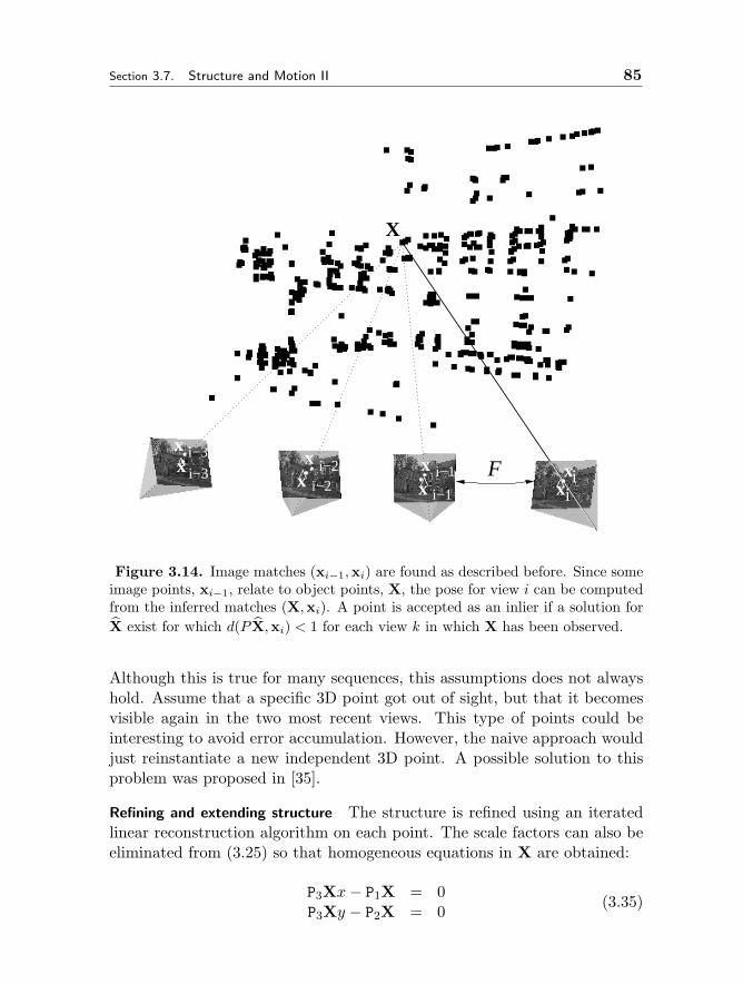
Section 3.7. Structure and Motion II 85
xi−3 x i−2 i−1 Fi−3
i−2i−1
x
X
xxx
x xi
i^
^^ ^
Figure 3.14. Image matches (xi−1,xi) are found as described before. Since someimage points, xi−1, relate to object points, X, the pose for view i can be computedfrom the inferred matches (X,xi). A point is accepted as an inlier if a solution forX exist for which d(P X,xi) < 1 for each view k in which X has been observed.
Although this is true for many sequences, this assumptions does not alwayshold. Assume that a specific 3D point got out of sight, but that it becomesvisible again in the two most recent views. This type of points could beinteresting to avoid error accumulation. However, the naive approach wouldjust reinstantiate a new independent 3D point. A possible solution to thisproblem was proposed in [35].
Refining and extending structure The structure is refined using an iteratedlinear reconstruction algorithm on each point. The scale factors can also beeliminated from (3.25) so that homogeneous equations in X are obtained:
P3Xx− P1X = 0P3Xy − P2X = 0
(3.35)
86 Multiple View Geometry Chapter 3
with Pi the i-th row of P and (x, y) being the image coordinates of the point.An estimate of X is computed by solving the system of linear equations ob-tained from all views where a corresponding image point is available. To ob-tain a better solution the criterion
∑d(PX,x)2 should be minimized. This
can be approximately obtained by iteratively solving the following weightedlinear least-squares problem:
1
P3X
[P3x− P1P3y − P2
]X = 0 (3.36)
where X is the previous solution for X. This procedure can be repeated afew times. By solving this system of equations through SVD a normalizedhomogeneous point is automatically obtained. If a 3D point is not observedthe position is not updated. In this case one can check if the point was seenin a sufficient number of views to be kept in the final reconstruction. Thisminimum number of views can for example be put to three. This avoids tohave an important number of outliers due to spurious matches.
Of course in an image sequence some new features will appear in everynew image. If point matches are available that were not related to an existingpoint in the structure, then a new point can be initialized as described inSection 3.7.2.
Refining structure and motion
Once the structure and motion has been obtained for the whole sequence,it is recommended to refine it through a global minimization step so that abias towards the initial views is avoided. A maximum likelihood estimationcan be obtained through bundle adjustment [67, 57]. The goal is to findthe parameters of the camera view Pk and the 3D points Xi for which thesum of squared distances between the observed image points mki and thereprojected image points Pk(Xi) is minimized. It is advised to extend thecamera projection model to also take radial distortion into account. For mviews and n points the following criterion should be minimized:
minPk,Xi
m∑k=1
n∑i=1
d(xki, Pk(Xi))2 (3.37)
If the errors on the localisation of image features are independent and satisfya zero-mean Gaussian distribution then it can be shown that bundle adjust-ment corresponds to a maximum likelihood estimator. This minimizationproblem is huge, e.g. for a sequence of 20 views and 100 points/view, a

Section 3.8. Auto-calibration 87
minimization problem in more than 6000 variables has to be solved (most ofthem related to the structure). A straight-forward computation is obviouslynot feasible. However, the special structure of the problem can be exploitedto solve the problem much more efficiently [67, 57]. The key reason for thisis that a specific residual is only dependent on one point and one camera,which results in a very sparse structure for the normal equations.
Structure and motion recovery algorithm
To conclude this section an overview of the structure and motion recoveryalgorithm is given. The whole procedure consists of the following steps:
1. Match or track points over the whole image sequence (see Section 3.5.2)
2. Initialize the structure and motion recovery
(a) Select two views that are suited for initialization(b) Set up the initial frame(c) Reconstruct the initial structure
3. For every additional view
(a) Infer matches to the existing 3D structure(b) Compute the camera pose using a robust algorithm(c) Refine the existing structure(d) Initialize new structure points
4. Refine the structure and motion through bundle adjustment
The results of this algorithm are the camera poses for all the views andthe reconstruction of the interest points. For most applications the cameraposes are the most usefull, e.g. MatchMoving (aligning a virtual camera withthe motion of a real camera, see Section 3.10.3).
3.8 Auto-calibration
As shown by Theorem 5, for a completely uncalibrated image sequence thereconstruction is only determined up to a projective transformation. Whileit is true that often the full calibration is not available, often some knowl-edge of the camera intrinsics is available. As will be seen in this section,this knowledge can be used to recover the structure and motion up to asimilarity transformation. This type of approach is called auto-calibration orself-calibration in the literature. A first class of algorithms assumes constant,
88 Multiple View Geometry Chapter 3
but unknown, intrinsic camera parameters [16, 21, 44, 28, 65]. Another classof algorithms assumes some intrinsic camera parameters to be known, whileothers can vary [47, 29]. Specific algorithms have also been proposed forrestricted camera motion, such as pure rotation [20, 11], or restricted scenestructure, such as planar scenes [66].
The absolute conic and its image
The central concept for auto-calibration is the absolute conic. As stated inProposition 3 the absolute conic allows to identify the similarity structure ina projective space. In other words, if, given a projective reconstruction, onewas able to locate the conic corresponding to the absolute conic in the realworld, this would be equivalent to recovering the structure of the observedscene up to a similarity. In this case, a transformation that transformsthe absolute conic to its canonical representation in Euclidean space, i.e.Ω′ = diag(1, 1, 1, 0), would yield a reconstruction similar to the original (i.e.identical up to orientation, position and scale).
As was seen in Proposition 6 the image of the absolute conic is directlyrelated to the intrinsic camera parameters, and this independently of thechoice of projective basis:
PΩ′P ∼ KK (3.38)
Therefore, constraints on the intrinsics can be used to constrain the loca-tion of the conic corresponding to the absolute conic. Most auto-calibrationalgorithms are based on (3.38).
Critical motion sequences
Auto-calibration is not always guaranteed to yield a uniqyue solution. De-pending on the available constraints on the intrinsics and on the cameramotion, the remaining ambiguity on the reconstruction might be larger thana similarity. This problem was identified as the problem of critical motionsequences. The first complete analysis of the problem for constant intrin-sics camera parameters was made by Sturm [61]. Analysis for some othercases can be found in [62, 43, 32]. It was also shown that in some cases theambiguity notwithstanding correct novel views could be generate [45].
Linear auto-calibration
In this section we present a simple linear algorithm for auto-calibration ofcameras. The approach, published in [49], is related to the initial approach
Section 3.8. Auto-calibration 89
published in [46], but avoids most of the problems due to critical motionsequences by incorporating more a priori knowledge. As input it requires aprojective representation of the camera projection matrices.
As discussed in Section 3.4.3, for most cameras it is reasonable to assumethat the pixels are close to square and that the principal point is close to thecenter of the image. The focal length (measured in pixel units) will typicallybe of the same order of magnitude as the image size. It is therefore a goodidea to perform the following normalization:
PN = K−1N P with KN =
w + h 0 w2
w + h h21
(3.39)
where w and h are the width, respectively height of the image. Afternormalization the focal length should be of the order of unity and the prin-cipal point should be close to the origin. The above normalization wouldscale a focal length of a 60mm lens to 1 and thus focal lengths in the rangeof 20mm to 180mm would end up in the range [1/3, 3] and the principalpoint should now be close to the origin. The aspect ratio is typically around1 and the skew can be assumed 0 for all practical purposes. Making thisa priori knowledge more explicit and estimating reasonable standard devia-tions yields f ≈ rf ≈ 1 ± 3, u ≈ v ≈ 0 ± 0.1, r ≈ 1 ± 0.1 and s = 0 whichapproximately translates to the following expectations for ω′:
ω′ ∼ KK =
γ2f2 + x20 x0y0 x0
x0y0 f2 + y20 y0
x0 y0 1
≈ 1± 9 ±0.01 ±0.1±0.01 1± 9 ±0.1±0.1 ±0.1 1
(3.40)
and ω′22/ω
′11 ≈ 1± 0.2. Now, these constraints can also be used to constrain
the left-hand side of (3.38). The uncertainty can be take into account byweighting the equations, yielding the following set of constraints:
ν9
(P1Ω′P1
− P3Ω′P3) = 0
ν9
(P2Ω′P2
− P3Ω′P3) = 0
ν0.2
(P1Ω′P1
− P2Ω′P2) = 0
ν0.1
(P1Ω′P2
) = 0ν
0.1
(P1Ω′P3
) = 0ν
0.01
(P2Ω′P3
) = 0
(3.41)
with Pi the ith row of P and ν a scale factor that can be set to 1. Iffor the solution P3Ω′P3
varies widely for the different views, one mightwant to iterate with ν = (P3Ω′P3
)−1 with Ω′ the result of the previous
90 Multiple View Geometry Chapter 3
iteration. Since Ω′ is a symmetric 4× 4 matrix it is linearly parametrized by10 coefficients. An estimate of the dual absolute quadric Ω′ can be obtainedby solving the above set of equations for all views through homogeneouslinear least-squares. The rank-3 constraint can be imposed by forcing thesmallest singular value to zero. The upgrading transformation T can beobtained from diag (1, 1, 1, 0) = TΩ′T by decomposition of Ω′.
Auto-calibration refinement
This result can then further be refined through bundle adjustment (see Sec-tion 3.7.2). In this case the constraints on the intrinsics should be enforcedduring the minimization process. Constraints on the intrinsics can be en-forced either exactly through parametrisation, or approximately by adding aresidual for the deviation from the expected value in the global minimizationprocess.
3.9 Dense Depth Estimation
With the camera calibration given for all viewpoints of the sequence, wecan proceed with methods developed for calibrated structure from motionalgorithms. The feature tracking algorithm already delivers a sparse sur-face model based on distinct feature points. This however is not sufficientto reconstruct geometrically correct and visually pleasing surface models.This task is accomplished by a dense disparity matching that estimates cor-respondences from the grey level images directly by exploiting additionalgeometrical constraints. The dense surface estimation is done in a numberof steps. First image pairs are rectified to the standard stereo configuration.Then disparity maps are computed through a stereo matching algorithm.Finally a multi-view approach integrates the results obtained from severalview pairs.
3.9.1 Rectification
Since the calibration between successive image pairs was computed, theepipolar constraint that restricts the correspondence search to a 1-D searchrange can be exploited. Image pairs can be warped so that epipolar linescoincide with image scan lines. The correspondence search is then reducedto a matching of the image points along each image scan-line. This resultsin a dramatic increase of the computational efficiency of the algorithms byenabling several optimizations in the computations.
For some motions (i.e. when the epipole is located in the image) standard
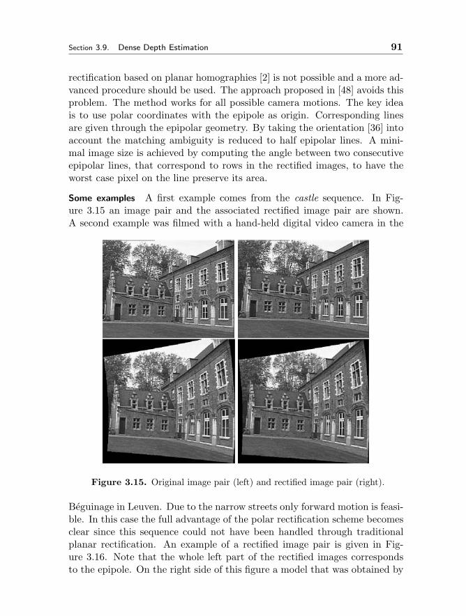
Section 3.9. Dense Depth Estimation 91
rectification based on planar homographies [2] is not possible and a more ad-vanced procedure should be used. The approach proposed in [48] avoids thisproblem. The method works for all possible camera motions. The key ideais to use polar coordinates with the epipole as origin. Corresponding linesare given through the epipolar geometry. By taking the orientation [36] intoaccount the matching ambiguity is reduced to half epipolar lines. A mini-mal image size is achieved by computing the angle between two consecutiveepipolar lines, that correspond to rows in the rectified images, to have theworst case pixel on the line preserve its area.
Some examples A first example comes from the castle sequence. In Fig-ure 3.15 an image pair and the associated rectified image pair are shown.A second example was filmed with a hand-held digital video camera in the
Figure 3.15. Original image pair (left) and rectified image pair (right).
Beguinage in Leuven. Due to the narrow streets only forward motion is feasi-ble. In this case the full advantage of the polar rectification scheme becomesclear since this sequence could not have been handled through traditionalplanar rectification. An example of a rectified image pair is given in Fig-ure 3.16. Note that the whole left part of the rectified images correspondsto the epipole. On the right side of this figure a model that was obtained by
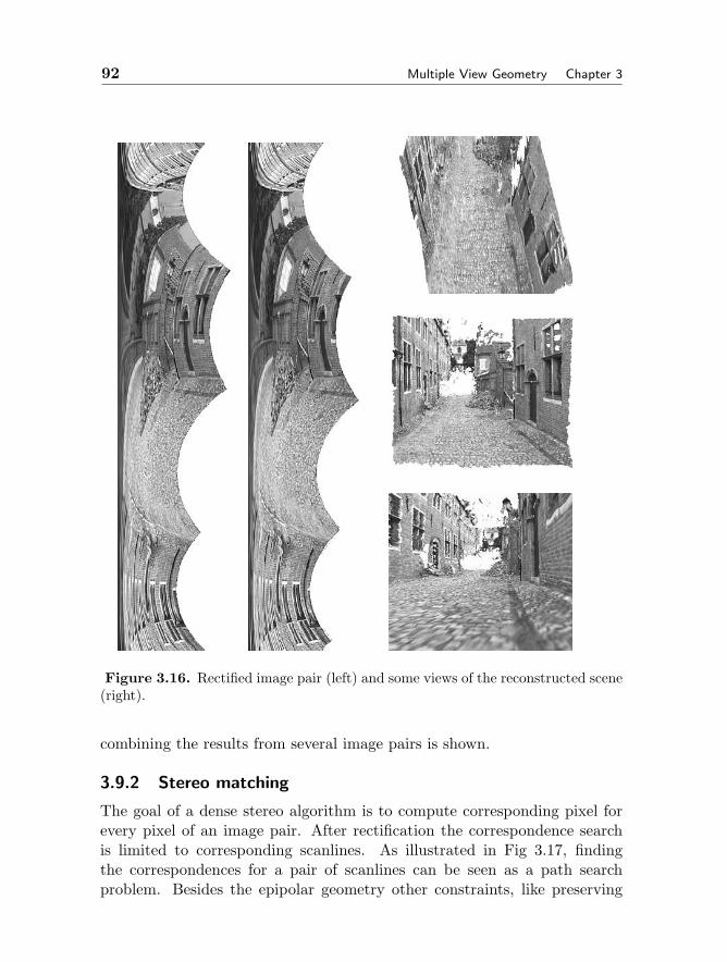
92 Multiple View Geometry Chapter 3
Figure 3.16. Rectified image pair (left) and some views of the reconstructed scene(right).
combining the results from several image pairs is shown.
3.9.2 Stereo matching
The goal of a dense stereo algorithm is to compute corresponding pixel forevery pixel of an image pair. After rectification the correspondence searchis limited to corresponding scanlines. As illustrated in Fig 3.17, findingthe correspondences for a pair of scanlines can be seen as a path searchproblem. Besides the epipolar geometry other constraints, like preserving

Section 3.9. Dense Depth Estimation 93
1 4
1 2 1,23,4 3 4
2 3
P Pk k+1
optim
al pa
th
epipolar line image k1 2 3,4
1,2 image l
searchregion
epip
olar
line
imag
e l
image kocclusion
occlusion
3
4
Figure 3.17. Illustration of the ordering constraint (left), dense matching as apath search problem (right).
the order of neighboring pixels, bidirectional uniqueness of the match, anddetection of occlusions can be exploited. In most cases it is also possibleto limit the search to a certain disparity range (an estimate of this rangecan be obtained from the reconstructed 3D feature points). Besides theseconstraints, a stereo algorithm should also take into account the similaritybetween corresponding points and the continuity of the surface. It is possibleto compute the optimal path taking all the constraints into account usingdynamic programming [8, 12, 41]. Other computationally more expensiveapproaches also take continuity across scanlines into account. Real-timeapproaches on the other hand estimate the best match independently forevery pixel. A complete taxonomy of stereo algorithms can be found in [52].
3.9.3 Multi-view linking
The pairwise disparity estimation allows to compute image to image corre-spondences between adjacent rectified image pairs, and independent depthestimates for each camera viewpoint. An optimal joint estimate is achievedby fusing all independent estimates into a common 3D model. The fusioncan be performed in an economical way through controlled correspondencelinking (see Figure 3.18). A point is transferred from one image to the nextas follows:
x2 = R′−1(R(x1) +D(R(x1)) (3.42)
with R(.) and R′(.) functions that map points from the original image intothe rectified image and D(.) a function that corresponds to the disparity
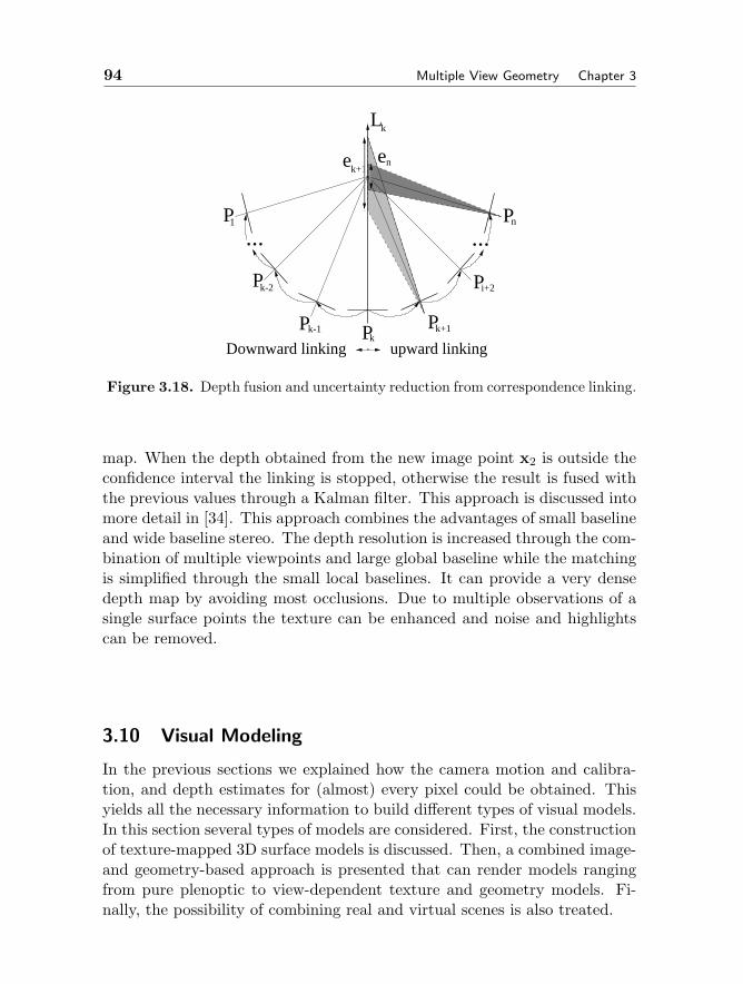
94 Multiple View Geometry Chapter 3
ne
kL
e
......P1
P Pi+2
nP
k+1
k+1P
k-2
Pk-1 PkDownward linking upward linking
Figure 3.18. Depth fusion and uncertainty reduction from correspondence linking.
map. When the depth obtained from the new image point x2 is outside theconfidence interval the linking is stopped, otherwise the result is fused withthe previous values through a Kalman filter. This approach is discussed intomore detail in [34]. This approach combines the advantages of small baselineand wide baseline stereo. The depth resolution is increased through the com-bination of multiple viewpoints and large global baseline while the matchingis simplified through the small local baselines. It can provide a very densedepth map by avoiding most occlusions. Due to multiple observations of asingle surface points the texture can be enhanced and noise and highlightscan be removed.
3.10 Visual Modeling
In the previous sections we explained how the camera motion and calibra-tion, and depth estimates for (almost) every pixel could be obtained. Thisyields all the necessary information to build different types of visual models.In this section several types of models are considered. First, the constructionof texture-mapped 3D surface models is discussed. Then, a combined image-and geometry-based approach is presented that can render models rangingfrom pure plenoptic to view-dependent texture and geometry models. Fi-nally, the possibility of combining real and virtual scenes is also treated.

Section 3.10. Visual Modeling 95
3.10.1 3D surface reconstruction
The 3D surface is approximated by a triangular mesh to reduce geometriccomplexity and to tailor the model to the requirements of computer graphicsvisualization systems. A simple approach consists of overlaying a 2D trian-gular mesh on top of one of the images and then build a corresponding 3Dmesh by placing the vertices of the triangles in 3D space according to thevalues found in the corresponding depth map. To reduce noise it is recom-mended to first smooth the depth image (the kernel can be chosen of thesame size as the mesh triangles). The image itself can be used as texturemap. While normally projective texture mapping would be required, thesmall size of the triangles allow to use standard (affine) texture mapping(the texture coordinates are trivially obtained as the 2D coordinates of thevertices).
Figure 3.19. Surface reconstruction approach (top): A triangular mesh is overlaidon top of the image. The vertices are back-projected in space according to the depthvalues. From this a 3D surface model is obtained (bottom)
96 Multiple View Geometry Chapter 3
It can happen that for some vertices no depth value is available or thatthe confidence is too low. In these cases the corresponding triangles arenot reconstructed. The same happens when triangles are placed over dis-continuities. This is achieved by selecting a maximum angle between thenormal of a triangle and the line-of-sight through its center (e.g. 85 de-grees). This simple approach works very well on the dense depth maps asobtained through multi-view linking. The surface reconstruction approachis illustrated in Figure 3.19.
A further example is shown in Figure 3.20. The video sequence wasrecorded with a hand-held camcorder on an archaeological site in Turkey(courtesy of Marc Waelkens). It shows a decorative medusa head that waspart of a monumental fountain. The video sequence was processed fullyautomatically by using the algorithms discussed in Section 3.7, 3.8, 3.9, 3.10.From the bundle adjustment and the multi-view linking, the accuracy wasestimated to be of 1
500 (compared to the size of the reconstructed object).This has to be compared with the image resolution of 720× 576. Note thatthe camera was uncalibrated and, besides the unknown focal length andprincipal point, has significant radial distortion and an aspect ratio differentfrom one, i.e. 1.09, which were all automatically recovered from the videosequence.
To reconstruct more complex shapes it is necessary to combine resultsfrom multiple depth maps. The simplest approach consists of generating sep-arate models independently and then loading them together in the graphicssystem. Since all depth-maps are located in a single coordinate frame, reg-istration is not an issue. Often it is interesting to integrate the differentmeshes into a single mesh. A possible approach is given in [10].
A further example is shown in Figure 3.20. The video sequence wasrecorded with a hand-held camcorder on the archaeological site of Sagalassoin Turkey (courtesy of Marc Waelkens). It shows a decorative medusa headthat was part of a monumental fountain. The video sequence was processedfully automatically by using the algorithms discussed in Section 3.7, 3.8, 3.9,3.10. From the bundle adjustment and the multi-view linking, the accuracywas estimated to be of 1
500 (compared to the size of the reconstructed object).This has to be compared with the image resolution of 720× 576. Note thatthe camera was uncalibrated and, besides the unknown focal length andprincipal point, has significant radial distortion and an aspect ratio differentfrom one, i.e. 1.09, which were all automatically recovered from the videosequence.
To reconstruct more complex shapes it is necessary to combine resultsfrom multiple depth maps. The simplest approach consists of generating sep-
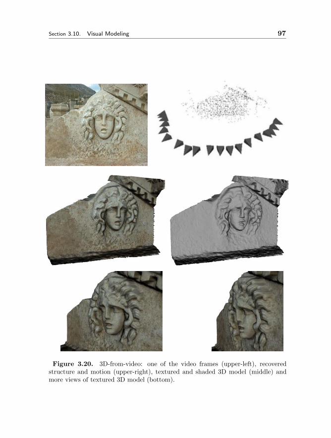
Section 3.10. Visual Modeling 97
Figure 3.20. 3D-from-video: one of the video frames (upper-left), recoveredstructure and motion (upper-right), textured and shaded 3D model (middle) andmore views of textured 3D model (bottom).
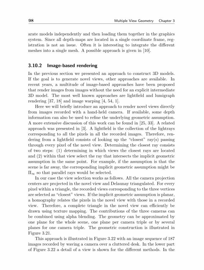
98 Multiple View Geometry Chapter 3
arate models independently and then loading them together in the graphicssystem. Since all depth-maps are located in a single coordinate frame, reg-istration is not an issue. Often it is interesting to integrate the differentmeshes into a single mesh. A possible approach is given in [10].
3.10.2 Image-based rendering
In the previous section we presented an approach to construct 3D models.If the goal is to generate novel views, other approaches are available. Inrecent years, a multitude of image-based approaches have been proposedthat render images from images without the need for an explicit intermediate3D model. The most well known approaches are lightfield and lumigraphrendering [37, 18] and image warping [4, 54, 1].
Here we will briefly introduce an approach to render novel views directlyfrom images recorded with a hand-held camera. If available, some depthinformation can also be used to refine the underlying geometric assumption.A more extensive discussion of this work can be found in [25, 33]. A relatedapproach was presented in [3]. A lightfield is the collection of the lightrayscorresponding to all the pixels in all the recorded images. Therefore, ren-dering from a lightfield consists of looking up the “closest” ray(s) passingthrough every pixel of the novel view. Determining the closest ray consistsof two steps: (1) determining in which views the closest rays are locatedand (2) within that view select the ray that intersects the implicit geometricassumption in the same point. For example, if the assumption is that thescene is far away, the corresponding implicit geometric assumption might beΠ∞ so that parallel rays would be selected.
In our case the view selection works as follows. All the camera projectioncenters are projected in the novel view and Delaunay triangulated. For everypixel within a triangle, the recorded views corresponding to the three verticesare selected as “closest” views. If the implicit geometric assumption is planar,a homography relates the pixels in the novel view with those in a recordedview. Therefore, a complete triangle in the novel view can efficiently bedrawn using texture mapping. The contributions of the three cameras canbe combined using alpha blending. The geometry can be approximated byone plane for the whole scene, one plane per camera triple or by severalplanes for one camera triple. The geometric construction is illustrated inFigure 3.21.
This approach is illustrated in Figure 3.22 with an image sequence of 187images recorded by waving a camera over a cluttered desk. In the lower partof Figure 3.22 a detail of a view is shown for the different methods. In the
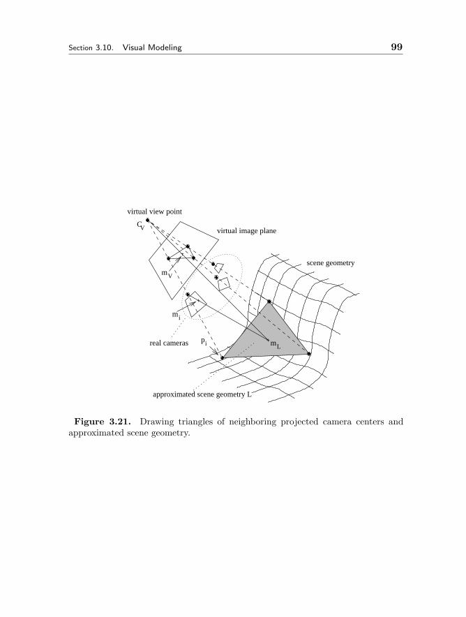
Section 3.10. Visual Modeling 99
mV
m
mLpi
i
virtual view point
virtual image plane
scene geometry
CV
real cameras
approximated scene geometry L
Figure 3.21. Drawing triangles of neighboring projected camera centers andapproximated scene geometry.
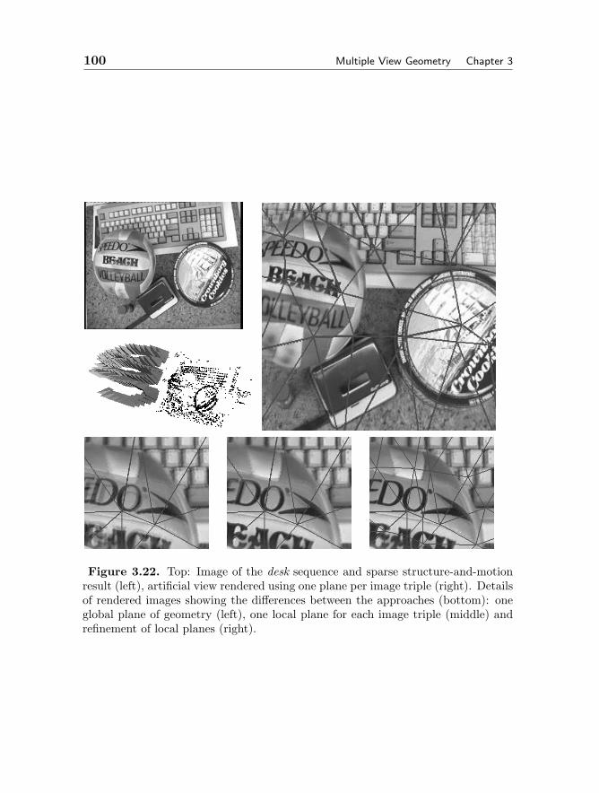
100 Multiple View Geometry Chapter 3
Figure 3.22. Top: Image of the desk sequence and sparse structure-and-motionresult (left), artificial view rendered using one plane per image triple (right). Detailsof rendered images showing the differences between the approaches (bottom): oneglobal plane of geometry (left), one local plane for each image triple (middle) andrefinement of local planes (right).
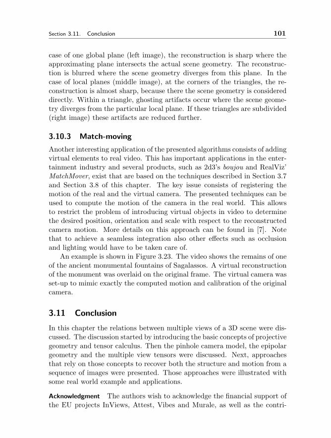
Section 3.11. Conclusion 101
case of one global plane (left image), the reconstruction is sharp where theapproximating plane intersects the actual scene geometry. The reconstruc-tion is blurred where the scene geometry diverges from this plane. In thecase of local planes (middle image), at the corners of the triangles, the re-construction is almost sharp, because there the scene geometry is considereddirectly. Within a triangle, ghosting artifacts occur where the scene geome-try diverges from the particular local plane. If these triangles are subdivided(right image) these artifacts are reduced further.
3.10.3 Match-moving
Another interesting application of the presented algorithms consists of addingvirtual elements to real video. This has important applications in the enter-tainment industry and several products, such as 2d3’s boujou and RealViz’MatchMover, exist that are based on the techniques described in Section 3.7and Section 3.8 of this chapter. The key issue consists of registering themotion of the real and the virtual camera. The presented techniques can beused to compute the motion of the camera in the real world. This allowsto restrict the problem of introducing virtual objects in video to determinethe desired position, orientation and scale with respect to the reconstructedcamera motion. More details on this approach can be found in [7]. Notethat to achieve a seamless integration also other effects such as occlusionand lighting would have to be taken care of.
An example is shown in Figure 3.23. The video shows the remains of oneof the ancient monumental fountains of Sagalassos. A virtual reconstructionof the monument was overlaid on the original frame. The virtual camera wasset-up to mimic exactly the computed motion and calibration of the originalcamera.
3.11 Conclusion
In this chapter the relations between multiple views of a 3D scene were dis-cussed. The discussion started by introducing the basic concepts of projectivegeometry and tensor calculus. Then the pinhole camera model, the epipolargeometry and the multiple view tensors were discussed. Next, approachesthat rely on those concepts to recover both the structure and motion from asequence of images were presented. Those approaches were illustrated withsome real world example and applications.
Acknowledgment The authors wish to acknowledge the financial support ofthe EU projects InViews, Attest, Vibes and Murale, as well as the contri-
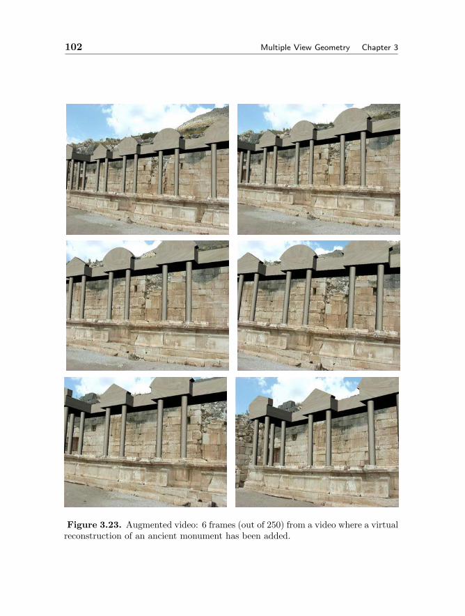
102 Multiple View Geometry Chapter 3
Figure 3.23. Augmented video: 6 frames (out of 250) from a video where a virtualreconstruction of an ancient monument has been added.
Bibliography 103
butions of their (former) colleagues in Leuven and Lund where most of thepresented work was carried out. Luc Van Gool, Maarten Vergauwen, FrankVerbiest, Kurt Cornelis, Jan Tops, Reinhard Koch and Benno Heigl havecontributed to generate the results that illustrate this chapter.
Bibliography
[1] S. Avidan and A. Shashua. Novel view synthesis in tensor space. In Proc. ofIEEE Conference on Computer Vision and Pattern Recognition, pages 1034–1040, 1997.
[2] N. Ayache. Artificial Vision for Mobile Robots: Stereo Vision and Multi-sensoryPerception. MIT Press, 1991.
[3] C. Buehler, M. Bosse, L. McMillan, S. Gortler, and M. Cohen. Unstructuredlumigraph rendering. In Proc. SIGGRAPH, 2001.
[4] S. Chen and L. Williams. View interpolation for image synthesis. ComputerGraphics, 27(Annual Conference Series):279–288, 1993.
[5] O. Chum and J. Matas. Randomized ransac and t(d,d) test. In Proc. BritishMachine Vision Conference, 2002.
[6] K. Cornelis, M. Pollefeys, M. Vergauwen, and L. Van Gool. Augmented realityfrom uncalibrated video sequences. In A. Zisserman M. Pollefeys, L. Van Gooland A. Fitzgibbon (Eds.), editors, 3D Structure from Images - SMILE 2000,volume 2018, pages 150–167. Springer-Verlag, 2001.
[7] K. Cornelis, M. Pollefeys, M. Vergauwen, F. Verbiest, and L. Van Gool. Track-ing based structure and motion recovery for augmented video productions.In Proceedings A.C.M. symposium on virtual reality software and technology- VRST 2001, pages 17–24, November 2001.
[8] I. Cox, S. Hingoraini, and S. Rao. A maximum likelihood stereo algorithm.Computer Vision and Image Understanding, 63(3):542–567, May 1996.
[9] H. S. M. Coxeter. Projective Geometry. Blaisdell Publishing Company, 1964.[10] B. Curless and M. Levoy. A volumetric method for building complex models
from range images. In Proc. SIGGRAPH ’96, pages 303–312, 1996.[11] L. de Agapito, R. Hartley, and E. Hayman. Linear selfcalibration of a rotating
and zooming camera. In Proc. IEEE Conf. Comp. Vision Patt. Recog., volume I,pages 15–21, June 1999.
[12] L. Falkenhagen. Depth estimation from stereoscopic image pairs assumingpiecewise continuous surfaces. In Proc. of European Workshop on combined Realand Synthetic Image Processing for Broadcast and Video Production, November1994.
[13] O. Faugeras. What can be seen in three dimensions with an uncalibrated stereorig? In Proc. European Conf. on Computer Vision, pages 563–578, 1992.
[14] O. Faugeras. Three-Dimensional Computer Vision. MIT Press, Cambridge,Mass., 1993.
[15] O. Faugeras and Q.-T. Luong. The Geometry of Multiple Images. MIT Press,Cambridge, Mass., 2001.
104 Multiple View Geometry Chapter 3
[16] O. Faugeras, Q.-T. Luong, and S. Maybank. Camera self-calibration: Theoryand experiments. In Computer Vision - ECCV’92, volume 588 of Lecture Notesin Computer Science, pages 321–334. Springer-Verlag, 1992.
[17] M. Fischler and R. Bolles. Random sampling consensus: a paradigm for modelfitting with application to image analysis and automated cartography. Com-mun. Assoc. Comp. Mach., 24:381–395, 1981.
[18] S. Gortler, R. Grzeszczuk, R. Szeliski, and M. F. Cohen. The lumigraph. InProc. SIGGRAPH ’96, pages 43–54. ACM Press, New York, 1996.
[19] C. Harris and M. Stephens. A combined corner and edge detector. In FourthAlvey Vision Conference, pages 147–151, 1988.
[20] R. Hartley. An algorithm for self calibration from several views. In Proc. IEEEConf. Comp. Vision Patt. Recog., pages 908–912, 1994.
[21] R. Hartley. Euclidean reconstruction from uncalibrated views. In J.L. Mundy,A. Zisserman, and D. Forsyth, editors, Applications of Invariance in Com-puter Vision, volume 825 of Lecture Notes in Computer Science, pages 237–256.Springer-Verlag, 1994.
[22] R. Hartley. In defense of the eight-point algorithm. IEEE Trans. on PatternAnalysis and Machine Intelligence, 19(6):580–593, June 1997.
[23] R. Hartley and P. Sturm. Triangulation. Computer Vision and Image Under-standing, 68(2):146–157, 1997.
[24] R. Hartley and A. Zisserman. Multiple View Geometry in Computer Vision.Cambridge University Press, 2000.
[25] B. Heigl, R. Koch, M. Pollefeys, J. Denzler, and L. Van Gool. Plenoptic mod-eling and rendering from image sequences taken by hand-held camera. In Proc.DAGM, pages 94–101, 1999.
[26] A. Heyden. Geometry and Algebra of Multipe Projective Transformations. PhDthesis, Lund University, Sweden, 1995.
[27] A. Heyden. Tensorial properties of multilinear constraints. Mathematical Meth-ods in the Applied Sciences, 23:169–202, 2000.
[28] A. Heyden and K. Astrom. Euclidean reconstruction from constant intrinsicparameters. In Proc. 13th International Conference on Pattern Recognition,pages 339–343. IEEE Computer Soc. Press, 1996.
[29] A. Heyden and K. Astrom. Euclidean reconstruction from image sequenceswith varying and unknown focal length and principal point. In Proc. IEEEConference on Computer Vision and Pattern Recognition, pages 438–443. IEEEComputer Soc. Press, 1997.
[30] A. Heyden and K. str m. Algebraic properties of multilinear constraints.Mathematical Methods in the Applied Sciences, 20:1135–1162, 1997.
[31] F. Kahl. Critical motions and ambiuous euclidean reconstructions in auto-calibration. In Proc. ICCV, pages 469–475, 1999.
[32] F. Kahl, B. Triggs, and K. Astrom. Critical motions for autocalibration whensome intrinsic parameters can vary. Jrnl. of Mathematical Imaging and Vision,13(2):131–146, 2000.
[33] R. Koch, B. Heigl, and M. Pollefeys. Image-based rendering from uncalibratedlightfields with scalable geometry. In G. Gimel’farb (Eds.) R. Klette, T. Huang,

Bibliography 105
editor, Multi-Image Analysis, volume 2032 of Lecture Notes in Computer Sci-ence, pages 51–66. Springer-Verlag, 2001.
[34] R. Koch, M. Pollefeys, and L. Van Gool. Multi viewpoint stereo from uncal-ibrated video sequences. In Proc. European Conference on Computer Vision,pages 55–71, 1998.
[35] R. Koch, M. Pollefeys, B. Heigl, L. Van Gool, and H. Niemann. Calibration ofhand-held camera sequences for plenoptic modeling. In Proc.ICCV’99 (inter-national Conference on Computer Vision), pages 585–591, 1999.
[36] S. Laveau and O. Faugeras. Oriented projective geometry for computer vision.In B. Buxton and R. Cipolla (eds.), editors, Computer Vision - ECCV’96,Lecture Notes in Computer Science, Vol. 1064, pages 147–156. Springer-Verlag,1996.
[37] M. Levoy and P. Hanrahan. Lightfield rendering. In Proc. SIGGRAPH ’96,pages 31–42. ACM Press, New York, 1996.
[38] H. C. Longuet-Higgins. A computer algorithm for reconstructing a scene fromtwo projections. Nature, 293:133–135, 1981.
[39] D. Lowe. Object recognition from local scale-invariant features. In Proc. Inter-national Conference on Computer Vision, pages 1150–1157, 1999.
[40] J. Matas, S. Obdrzalek, and O. Chum. Local affine frames for wide-baselinestereo. In Proc. 16th International Conference on Pattern Recognition, vol-ume 4, pages 363–366, 2002.
[41] G. Van Meerbergen, M. Vergauwen, M. Pollefeys, and L. Van Gool. A hierar-chical symmetric stereo algorithm using dynamic programming. InternationalJournal on Computer Vision, 47(1/2/3):275–285, 2002.
[42] N. Myklestad. Cartesian Tensors - the Mathematical Language of Engineering.Van Nostrand, Princeton, 1967.
[43] M. Pollefeys. Self-calibration and metric 3D reconstruction from uncalibratedimage sequences. PhD thesis, Katholieke Universiteit Leuven, 1999.
[44] M. Pollefeys and L. Van Gool. Stratified self-calibration with the modulusconstraint. IEEE transactions on Pattern Analysis and Machine Intelligence,21(8):707–724, 1999.
[45] M. Pollefeys and Luc Van Gool. Do ambiguous reconstructions always giveambiguous images? In Proc. International Conference on Computer Vision,pages 187–192, 2001.
[46] M. Pollefeys, R. Koch, and L. Van Gool. Self-calibration and metric recon-struction in spite of varying and unknown internal camera parameters. In Proc.International Conference on Computer Vision, pages 90–95. Narosa PublishingHouse, 1998.
[47] M. Pollefeys, R. Koch, and L. Van Gool. Self-calibration and metric reconstruc-tion in spite of varying and unknown internal camera parameters. InternationalJournal of Computer Vision, 32(1):7–25, 1999.
[48] M. Pollefeys, R. Koch, and L. Van Gool. A simple and efficient rectificationmethod for general motion. In Proc.ICCV’99 (international Conference onComputer Vision), pages 496–501, 1999.

106 Multiple View Geometry Chapter 3
[49] M. Pollefeys, F. Verbiest, and L. Van Gool. Surviving dominant planes in uncal-ibrated structure and motion recovery. In A. Heyden, G. Sparr, M. Nielsen, andP. Johansen, editors, Computer Vision - ECCV 2002, 7th European Conferenceon Computer Vision, volume 2351 of Lecture Notes in Computer Science, pages837–851, 2002.
[50] W. Press, S. Teukolsky, and W. Vetterling. Numerical recipes in C: the art ofscientific computing. Cambridge university press, 1992.
[51] P. Rousseeuw. Robust Regression and Outlier Detection. Wiley, New York,1987.
[52] D. Scharstein and R. Szeliski. A taxonomy and evaluation of dense two-framestereo correspondence algorithms. International Journal of Computer Vision,47(1/2/3):7–42, April-June 2002.
[53] C. Schmid and R. Mohr. Local grayvalue invariants for image retrieval. IEEEPAMI, 19(5):530–534, 1997.
[54] S. Seitz and C. Dyer. View morphing. Computer Graphics, 30(Annual Confer-ence Series):21–30, 1996.
[55] A. Shashua. Trilinearity in visual recognition by alignment. In Proc. EuropeanConf. on Computer Vision, 1994.
[56] J. Shi and C. Tomasi. Good features to track. In Proc. IEEE Conference onComputer Vision and Pattern Recognition (CVPR’94), pages 593–600, 1994.
[57] C. Slama. Manual of Photogrammetry. American Society of Photogrammetry,Falls Church, VA, USA, 4 edition, 1980.
[58] B. Spain. Tensor Calculus. University Mathematical Texts, Oliver and Boyd,Edingburgh, 1953.
[59] G. Sparr. Simultaneous reconstruction of scene structure and camera locationsfrom uncalibrated image sequences. In Proc. International Conf. on PatternRecognition, 1996.
[60] M. E. Spetsakis and J. Aloimonos. A unified theory of structure from motion.In Proc. DARPA IU Workshop, 1990.
[61] P. Sturm. Critical motion sequences for monocular self-calibration and uncali-brated euclidean reconstruction. In Proc. 1997 Conference on Computer Visionand Pattern Recognition, pages 1100–1105. IEEE Computer Soc. Press, 1997.
[62] P. Sturm. Critical motion sequences for the self-calibration of cameras andstereo systems with variable focal length. In Proc. 10th British Machine VisionConference, pages 63–72, 1999.
[63] P. Sturm. Critical motion sequences for the self-calibration of cameras andstereo systems with variable focal length. In Proc. BMVC, 1999.
[64] B. Triggs. Matching constraints and the joint image. In Proc. Int. Conf. onComputer Vision, 1995.
[65] B. Triggs. The absolute quadric. In Proc. 1997 Conference on Computer Visionand Pattern Recognition, pages 609–614. IEEE Computer Soc. Press, 1997.
[66] B. Triggs. Autocalibration from planar scenes. In ECCV, volume I, pages89–105, June 1998.
[67] B. Triggs, P. McLauchlan, R. Hartley, and A. Fiztgibbon. Bundle adjustment –a modern synthesis. In R. Szeliski (Eds.) B. Triggs, A. Zisserman, editor, Vision

Bibliography 107
Algorithms: Theory and Practice, LNCS Vol.1883, pages 298–372. Springer-Verlag, 2000.
[68] G. Turk and M. Levoy. Zippered polygon meshes from range images. In Pro-ceedings of SIGGRAPH ’94, pages 311–318, 1994.
[69] T. Tuytelaars and L. Van Gool. Wide baseline stereo based on local, affinelyinvariant regions. In British Machine Vision Conference, pages 412–422, 2000.
[70] Z. Zhang, R. Deriche, O. Faugeras, and Q.-T. Luong. A robust techniquefor matching two uncalibrated images through the recovery of the unknownepipolar geometry. Artificial Intelligence Journal, 78:87–119, October 1995.

Chapter 4
ROBUST TECHNIQUES FORCOMPUTER VISION
Peter Meer
4.1 Robustness in Visual Tasks
Visual information makes up about seventy five percent of all the senso-rial information received by a person during a lifetime. This informationis processed not only efficiently but also transparently. Our awe of visualperception was perhaps the best captured by the seventeenth century britishessayist Joseph Addison in an essay on imagination [1].
Our sight is the most perfect and most delightful of all our senses.It fills the mind with the largest variety of ideas, converses withits objects at the greatest distance, and continues the longest inaction without being tired or satiated with its proper enjoyments.
The ultimate goal of computer vision is to mimic human visual per-ception. Therefore, in the broadest sense, robustness of a computer visionalgorithm is judged against the performance of a human observer performingan equivalent task. In this context, robustness is the ability to extract thevisual information of relevance for a specific task, even when this informationis carried only by a small subset of the data, and/or is significantly differentfrom an already stored representation.
To understand why the performance of generic computer vision algo-rithms is still far away from that of human visual perception, we shouldconsider the hierarchy of computer vision tasks. They can be roughly clas-sified into three large categories:
109
110 Robust Techniques for Computer Vision Chapter 4
– low level, dealing with extraction from a single image of salient simplefeatures, such as edges, corners, homogeneous regions, curve fragments;
– intermediate level, dealing with extraction of semantically relevantcharacteristics from one or more images, such as grouped features,depth, motion information;
– high level, dealing with the interpretation of the extracted information.A similar hierarchy is difficult to distinguish in human visual perception,which appears as a single integrated unit. In the visual tasks performed bya human observer an extensive top-down information flow carrying repre-sentations derived at higher levels seems to control the processing at lowerlevels. See [84] for a discussion on the nature of these interactions.
A large amount of psychophysical evidence supports this “closed loop”model of human visual perception. Preattentive vision phenomena, in whichsalient information pops-out from the image, e.g., [55], [109], or perceptualconstancies, in which changes in the appearance of a familiar object areattributed to external causes [36, Chap.9], are only some of the examples.Similar behavior is yet to be achieved in generic computer vision techniques.For example, preattentive vision type processing seems to imply that a regionof interest is delineated before extracting its salient features.
To approach the issue of robustness in computer vision, will start bymentioning one of the simplest perceptual constancies, the shape constancy.Consider a door opening in front of an observer. As the door opens, itsimage changes from a rectangle to a trapezoid but the observer will reportonly the movement. That is, additional information not available in theinput data was also taken into account. We know that a door is a rigidstructure, and therefore it is very unlikely that its image changed due toa nonrigid transformation. Since the perceptual constancies are based onrules embedded in the visual system, they can be also deceived. A wellknown example is the Ames room in which the rules used for perspectiveforeshortening compensation are violated [36, p.241].
The previous example does not seem to reveal much. Any computervision algorithm of rigid motion recovery is based on a similar approach.However, the example emphasizes that the employed rigid motion model isonly associated with the data and is not intrinsic to it. We could use acompletely different model, say of nonrigid doors, but the result would notbe satisfactory. Robustness thus is closely related to the availability of amodel adequate for the goal of the task.
In today’s computer vision algorithms the information flow is almost ex-clusively bottom-up. Feature extraction is followed by grouping into seman-
Section 4.1. Robustness in Visual Tasks 111
tical primitives, which in turn is followed by a task specific interpretation ofthe ensemble of primitives. The lack of top-down information flow is arguablythe main reason why computer vision techniques cannot yet autonomouslyhandle visual data under a wide range of operating conditions. This factis well understood in the vision community and different approaches wereproposed to simulate the top-down information stream.
The increasingly popular Bayesian paradigm is such an attempt. Byusing a probabilistic representation for the possible outcomes, multiple hy-potheses are incorporated into the processing, which in turn guide the infor-mation recovery. The dependence of the procedure on the accuracy of theemployed representation is relaxed in the semiparametric or nonparametricBayesian methods, such as particle filtering for motion problems [51]. In-corporating a learning component into computer vision techniques, e.g., [3],[29], is another, somewhat similar approach to use higher level informationduring the processing.
Comparison with human visual perception is not a practical way to arriveto a definition of robustness for computer vision algorithms. For example,robustness in the context of the human visual system extends to abstractconcepts. We can recognize a chair independent of its design, size or theperiod in which it was made. However, in a somewhat similar experiment,when an object recognition system was programmed to decide if a simpledrawing represents a chair, the results were rather mixed [96].
We will not consider high level processes when examining the robustnessof vision algorithms, neither will discuss the role of top-down informationflow. A computer vision algorithm will be called robust if it can tolerateoutliers, i.e., data which does not obey the assumed model. This definitionis similar to the one used in statistics for robustness [40, p.6]
In a broad informal sense, robust statistics is a body of knowl-edge, partly formalized into “theories of statistics,” relating todeviations from idealized assumptions in statistics.
Robust techniques are used in computer vision for at least thirty years.In fact, those most popular today are related to old methods proposed tosolve specific image understanding or pattern recognition problems. Some ofthem were rediscovered only in the last few years.
The best known example is the Hough transform, a technique to extractmultiple instances of a low-dimensional manifold from a noisy background.The Hough transform is a US Patent granted in 1962 [47] for the detectionof linear trajectories of subatomic particles in a bubble chamber. In therare cases when Hough transform is explicitly referenced this patent is used,
112 Robust Techniques for Computer Vision Chapter 4
though an earlier publication also exists [46]. Similarly, the most popularrobust regression methods today in computer vision belong to the family ofrandom sample consensus (RANSAC), proposed in 1980 to solve the per-spective n-point problem [25]. The usually employed reference is [26]. Anold pattern recognition technique for density gradient estimation proposed in1975 [32], the mean shift, recently became a widely used methods for featurespace analysis. See also [31, p.535].
In theoretical statistics, investigation of robustness started in the early1960s, and the first robust estimator, the M-estimator, was introduced byHuber in 1964. See [49] for the relevant references. Another popular familyof robust estimators, including the least median of squares (LMedS), wasintroduced by Rousseeuw in 1984 [86]. By the end of 1980s these robusttechniques became known in the computer vision community.
Application of robust methods to vision problems was restricted at thebeginning to replacing a nonrobust parameter estimation module with itsrobust counterpart, e.g., [4], [41], [59], [102]. See also the review paper [74].While this approach was successful in most of the cases, soon also somefailures were reported [77]. Today we know that these failures are due to theinability of most robust estimators to handle data in which more than onestructure is present [9], [97], a situation frequently met in computer visionbut almost never in statistics. For example, a window operator often coversan image patch which contains two homogeneous regions of almost equalsizes, or there can be several independently moving objects in a visual scene.
Large part of today’s robust computer vision toolbox is indigenous. Thereare good reasons for this. The techniques imported from statistics weredesigned for data with characteristics significantly different from that of thedata in computer vision. If the data does not obey the assumptions impliedby the method of analysis, the desired performance may not be achieved.The development of robust techniques in the vision community (such asRANSAC) were motivated by applications. In these techniques the user hasmore freedom to adjust the procedure to the specific data than in a similartechnique taken from the statistical literature (such as LMedS). Thus, someof the theoretical limitations of a robust method can be alleviated by dataspecific tuning, which sometimes resulted in attributing better performanceto a technique than is theoretically possible in the general case.
A decade ago, when a vision task was solved with a robust technique, thefocus of the research was on the methodology and not on the application.Today the emphasis has changed, and often the employed robust techniquesare barely mentioned. It is no longer of interest to have an exhaustive surveyof “robust computer vision”. For some representative results see the review
Section 4.2. Models and Estimation Problems 113
paper [98] or the special issue [94].The goal of this chapter is to focus on the theoretical foundations of the
robust methods in the context of computer vision applications. We will pro-vide a unified treatment for most estimation problems, and put the emphasison the underlying concepts and not on the details of implementation of aspecific technique. Will describe the assumptions embedded in the differentclasses of robust methods, and clarify some misconceptions often arising inthe vision literature. Based on this theoretical analysis new robust methods,better suited for the complexity of computer vision tasks, can be designed.
4.2 Models and Estimation Problems
In this section we examine the basic concepts involved in parameter esti-mation. We describe the different components of a model and show how tofind the adequate model for a given computer vision problem. Estimation isanalyzed as a generic problem, and the differences between nonrobust androbust methods are emphasized. We also discuss the role of the optimizationcriterion in solving an estimation problem.
4.2.1 Elements of a Model
The goal of data analysis is to provide for data spanning a very high-dimensional space an equivalent low-dimensional representation. A set ofmeasurements consisting of n data vectors yi ∈ Rq can be regarded as apoint in Rnq. If the data can be described by a model with only p nqparameters, we have a much more compact representation. Should new datapoints become available, their relation to the initial data then can be estab-lished using only the model. A model has two main components
– the constraint equation;
– the measurement equation.The constraint describes our a priori knowledge about the nature of theprocess generating the data, while the measurement equation describes theway the data was obtained.
In the general case a constraint has two levels. The first level is thatof the quantities providing the input into the estimation. These variablesy1, . . . , yq can be obtained either by direct measurement or can be theoutput of another process. The variables are grouped together in the contextof the process to be modeled. Each ensemble of values for the q variablesprovides a single input data point, a q-dimensional vector y ∈ Rq.
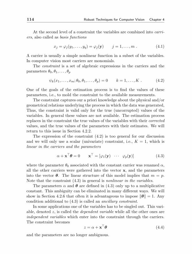
114 Robust Techniques for Computer Vision Chapter 4
At the second level of a constraint the variables are combined into carri-ers, also called as basis functions
xj = ϕj(y1, . . . , yq) = ϕj(y) j = 1, . . . ,m . (4.1)
A carrier is usually a simple nonlinear function in a subset of the variables.In computer vision most carriers are monomials.
The constraint is a set of algebraic expressions in the carriers and theparameters θ0, θ1, . . . , θp
ψk(x1, . . . , xm; θ0, θ1, . . . , θp) = 0 k = 1, . . . ,K . (4.2)
One of the goals of the estimation process is to find the values of theseparameters, i.e., to mold the constraint to the available measurements.
The constraint captures our a priori knowledge about the physical and/orgeometrical relations underlying the process in which the data was generated,Thus, the constraint is valid only for the true (uncorrupted) values of thevariables. In general these values are not available. The estimation processreplaces in the constraint the true values of the variables with their correctedvalues, and the true values of the parameters with their estimates. We willreturn to this issue in Section 4.2.2.
The expression of the constraint (4.2) is too general for our discussionand we will only use a scalar (univariate) constraint, i.e., K = 1, which islinear in the carriers and the parameters
α+ xθ = 0 x = [ϕ1(y) · · · ϕp(y)] (4.3)
where the parameter θ0 associated with the constant carrier was renamed α,all the other carriers were gathered into the vector x, and the parametersinto the vector θ. The linear structure of this model implies that m = p.Note that the constraint (4.3) in general is nonlinear in the variables.
The parameters α and θ are defined in (4.3) only up to a multiplicativeconstant. This ambiguity can be eliminated in many different ways. We willshow in Section 4.2.6 that often it is advantageous to impose ‖θ‖ = 1. Anycondition additional to (4.3) is called an ancillary constraint.
In some applications one of the variables has to be singled out. This vari-able, denoted z, is called the dependent variable while all the other ones areindependent variables which enter into the constraint through the carriers.The constraint becomes
z = α+ xθ (4.4)
and the parameters are no longer ambiguous.
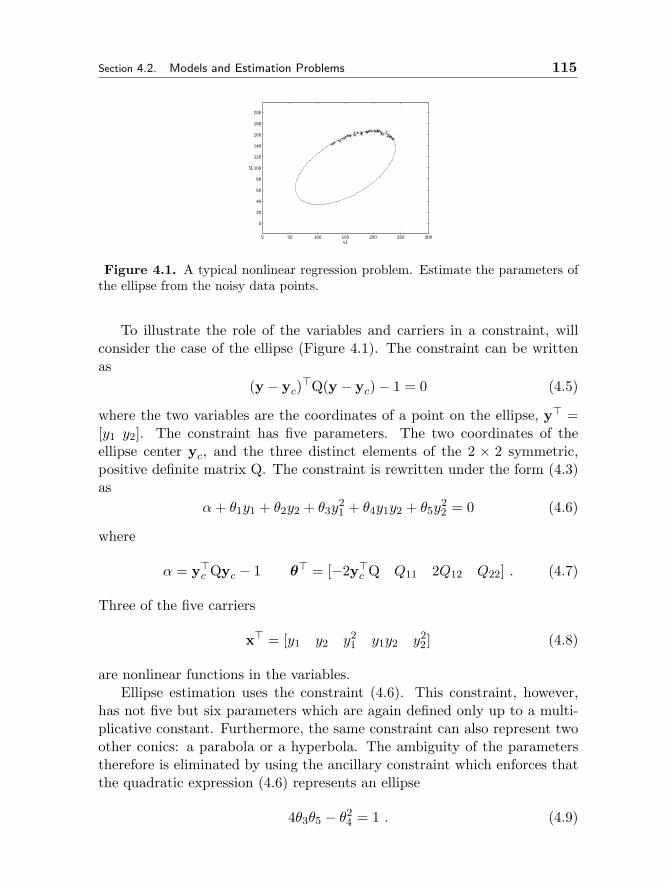
Section 4.2. Models and Estimation Problems 115
0 50 100 150 200 250 300
0
20
40
60
80
100
120
140
160
180
200
y1
y2
Figure 4.1. A typical nonlinear regression problem. Estimate the parameters ofthe ellipse from the noisy data points.
To illustrate the role of the variables and carriers in a constraint, willconsider the case of the ellipse (Figure 4.1). The constraint can be writtenas
(y − yc)Q(y − yc)− 1 = 0 (4.5)
where the two variables are the coordinates of a point on the ellipse, y =[y1 y2]. The constraint has five parameters. The two coordinates of theellipse center yc, and the three distinct elements of the 2 × 2 symmetric,positive definite matrix Q. The constraint is rewritten under the form (4.3)as
α+ θ1y1 + θ2y2 + θ3y21 + θ4y1y2 + θ5y
22 = 0 (4.6)
where
α = yc Qyc − 1 θ = [−2y
c Q Q11 2Q12 Q22] . (4.7)
Three of the five carriers
x = [y1 y2 y21 y1y2 y2
2] (4.8)
are nonlinear functions in the variables.Ellipse estimation uses the constraint (4.6). This constraint, however,
has not five but six parameters which are again defined only up to a multi-plicative constant. Furthermore, the same constraint can also represent twoother conics: a parabola or a hyperbola. The ambiguity of the parameterstherefore is eliminated by using the ancillary constraint which enforces thatthe quadratic expression (4.6) represents an ellipse
4θ3θ5 − θ24 = 1 . (4.9)
116 Robust Techniques for Computer Vision Chapter 4
The nonlinearity of the constraint in the variables makes ellipse estimationa difficult problem. See [27], [57], [72], [117] for different approaches anddiscussions.
For most of the variables only the noise corrupted version of their truevalue is available. Depending on the nature of the data, the noise is dueto the measurement errors, or to the inherent uncertainty at the outputof another estimation process. While for convenience we will use the termmeasurements for any input into an estimation process, the above distinctionabout the origin of the data should be kept in mind.
The general assumption in computer vision problems is that the noise isadditive. Thus, the measurement equation is
yi = yio + δyi yi ∈ Rq i = 1, . . . , n (4.10)
where yio is the true value of yi, the i-th measurement. The subscript ‘o’denotes the true value of a measurement. Since the constraints (4.3) or (4.4)capture our a priori knowledge, they are valid for the true values of themeasurements or parameters, and should have been written as
α+ xo θ = 0 or zo = α+ x
o θ (4.11)
where xo = x(yo). In the ellipse example y1o and y2o should have been usedin (4.6).
The noise corrupting the measurements is assumed to be independentand identically distributed (i.i.d.)
δyi ∼ GI(0, σ2Cy) (4.12)
where GI(·) stands for a general symmetric distribution of independent out-comes. Note that this distribution does not necessarily has to be normal. Awarning is in order, though. By characterizing the noise only with its firsttwo central moments we implicitly agree to normality, since only the normaldistribution is defined uniquely by these two moments.
The independency assumption usually holds when the input data pointsare physical measurements, but may be violated when the data is the outputof another estimation process. It is possible to take into account the corre-lation between two data points yi and yj in the estimation, e.g., [75], but itis rarely used in computer vision algorithm. Most often this is not a crucialomission since the main source of performance degradation is the failure ofthe constraint to adequately model the structure of the data.
The covariance of the noise is the product of two components in (4.12).The shape of the noise distribution is determined by the matrix Cy. This
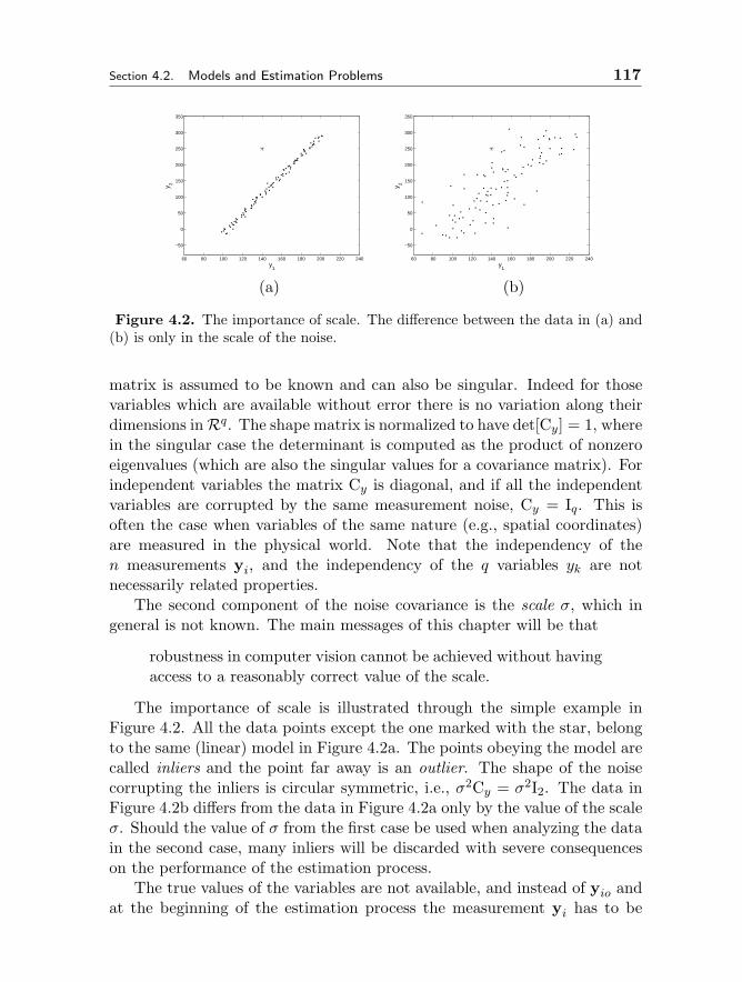
Section 4.2. Models and Estimation Problems 117
60 80 100 120 140 160 180 200 220 240
−50
0
50
100
150
200
250
300
350
y1
y 2
60 80 100 120 140 160 180 200 220 240
−50
0
50
100
150
200
250
300
350
y1
y 2
(a) (b)
Figure 4.2. The importance of scale. The difference between the data in (a) and(b) is only in the scale of the noise.
matrix is assumed to be known and can also be singular. Indeed for thosevariables which are available without error there is no variation along theirdimensions inRq. The shape matrix is normalized to have det[Cy] = 1, wherein the singular case the determinant is computed as the product of nonzeroeigenvalues (which are also the singular values for a covariance matrix). Forindependent variables the matrix Cy is diagonal, and if all the independentvariables are corrupted by the same measurement noise, Cy = Iq. This isoften the case when variables of the same nature (e.g., spatial coordinates)are measured in the physical world. Note that the independency of then measurements yi, and the independency of the q variables yk are notnecessarily related properties.
The second component of the noise covariance is the scale σ, which ingeneral is not known. The main messages of this chapter will be that
robustness in computer vision cannot be achieved without havingaccess to a reasonably correct value of the scale.
The importance of scale is illustrated through the simple example inFigure 4.2. All the data points except the one marked with the star, belongto the same (linear) model in Figure 4.2a. The points obeying the model arecalled inliers and the point far away is an outlier. The shape of the noisecorrupting the inliers is circular symmetric, i.e., σ2Cy = σ2I2. The data inFigure 4.2b differs from the data in Figure 4.2a only by the value of the scaleσ. Should the value of σ from the first case be used when analyzing the datain the second case, many inliers will be discarded with severe consequenceson the performance of the estimation process.
The true values of the variables are not available, and instead of yio andat the beginning of the estimation process the measurement yi has to be
118 Robust Techniques for Computer Vision Chapter 4
used to compute the carriers. The first two central moments of the noiseassociated with a carrier can be approximated by error propagation.
Let xij = ϕj(yi) be the j-th element, j = 1, . . . , p, of the carrier vectorxi = x(yi) ∈ Rp, computed for the i-th measurement yi ∈ Rq, i = 1, . . . , n.Since the measurement vectors yi are assumed to be independent, the carriervectors xi are also independent random variables.
The second order Taylor expansion of the carrier xij around the corre-sponding true value xijo = ϕj(yio) is
xij ≈ xijo+[∂ϕj(yio)∂y
](yi−yio)+
12(yi−yio)
∂2ϕj(yio)∂y∂y (yi−yio) (4.13)
where ∂ϕj(yio)∂y is the gradient of the carrier with respect to the vector of the
variables y, and Hj(yio) = ∂2ϕj(yio)∂y∂y is its Hessian matrix, both computed in
the true value of the variables yio. From the measurement equation (4.10)and (4.13) the second order approximation for the expected value of the noisecorrupting the carrier xij is
E[xij − xijo] =σ2
2trace[CyHj(yio)] (4.14)
which shows that this noise is not necessarily zero-mean. The first order ap-proximation of the noise covariance obtained by straightforward error prop-agation
cov[xi − xio] = σ2Cxi = σ2Jx|y(yio)CyJx|y(yio) (4.15)
where Jx|y(yio) is the Jacobian of the carrier vector x with respect to thevector of the variables y, computed in the true values yio. In general themoments of the noise corrupting the carriers are functions of yio and thus arepoint dependent. A point dependent noise process is called heteroscedastic.Note that the dependence is through the true values of the variables, whichin general are not available. In practice, the true values are substituted withthe measurements.
To illustrate the heteroscedasticity of the carrier noise we return to theexample of the ellipse. From (4.8) we obtain the Jacobian
Jx|y =[
1 0 2y1 y2 00 1 0 y1 2y2
](4.16)
and the Hessians
H1 = H2 = 0 H3 =[
2 00 0
]H4 =
[0 11 0
]H5 =
[0 00 2
]. (4.17)
Section 4.2. Models and Estimation Problems 119
Assume that the simplest measurement noise distributed GI(0, σ2I2) is cor-rupting the two spatial coordinates (the variables). The noise corrupting thecarriers, however, has nonzero mean and a covariance which is a function ofyo
E[x− xo] = [0 0 σ2 0 σ2] cov[x− xo] = σ2Jx|y(yo)Jx|y(yo) .
(4.18)To accurately estimate the parameters of the general model the heteroscedas-ticity of the carrier noise has to be taken into account, as will be discussedin Section 4.2.5.
4.2.2 Estimation of a Model
We can proceed now to a formal definition of the estimation process.
Given the model:– the noisy measurements yi which are the additively corrupted
versions of the true values yio
yi = yio + δyi yi ∈ Rq δyi ∼ GI(0, σ2Cy) i = 1, . . . , n
– the covariance of the errors σ2Cy, known only up to the scale σ
– the constraint obeyed by the true values of the measurements
α+ xioθ = 0 xio = x(yio) i = 1, . . . , n
and some ancillary constraints.
Find the estimates:– for the model parameters, α and θ
– for the true values of the measurements, yi– such that they satisfy the constraint
α+ xi θ = 0 xi = x(yi) i = 1, . . . , n
and all the ancillary constraints.
The true values of the measurements yio are called nuisance parameterssince they have only a secondary role in the estimation process. We willtreat the nuisance parameters as unknown constants, in which case we havea functional model [33, p.2]. When the nuisance parameters are assumed toobey a know distribution whose parameters also have to be estimated, we
120 Robust Techniques for Computer Vision Chapter 4
have a structural model. For robust estimation the functional models aremore adequate since require less assumptions about the data.
The estimation of a functional model has two distinct parts. First, theparameter estimates are obtained in the main parameter estimation proce-dure, followed by the computation of the nuisance parameter estimates in thedata correction procedure. The nuisance parameter estimates yi are calledthe corrected data points. The data correction procedure is usually not morethan the projection of the measurements yi on the already estimated con-straint surface.
The parameter estimates are obtained by (most often) seeking the globalminima of an objective function. The variables of the objective function arethe normalized distances between the measurements and their true values.They are defined from the squared Mahalanobis distances
d2i =
1σ2 (yi − yio)
C+y (yi − yio) =
1σ2 δy
i C+
y δyi i = 1, . . . , n (4.19)
where ‘+’ stands for the pseudoinverse operator since the matrix Cy canbe singular, in which case (4.19) is only a pseudodistance. Note that di ≥0. Through the estimation procedure the yio are replaced with yi and thedistance di becomes the absolute value of the normalized residual.
The objective function J (d1, . . . , dn) is always a positive semidefinitefunction taking value zero only when all the distances are zero. We shoulddistinguish between homogeneous and nonhomogeneous objective functions.A homogeneous objective function has the property
J (d1, . . . , dn) =1σJ (‖δy1‖Cy
, . . . , ‖δyn‖Cy) (4.20)
where ‖δyi‖Cy= [δy
i C+y δyi]
1/2 is the covariance weighted norm of the mea-surement error. The homogeneity of an objective function is an importantproperty in the estimation. Only for homogeneous objective functions wehave
[ α, θ ] = argminα,θJ (d1, . . . , dn) = argmin
α,θJ(‖δy1‖Cy
, . . . , ‖δyn‖Cy
)(4.21)
meaning that the scale σ does not play any role in the main estimationprocess. Since the value of the scale is not known a priori, by removingit an important source for performance deterioration is eliminated. All thefollowing objective functions are homogeneous
JLS =1n
n∑i=1
d2i JLAD =
1n
n∑i=1
di JLkOS = dk:n (4.22)
Section 4.2. Models and Estimation Problems 121
where, JLS yields the family of least squares estimators, JLAD the least abso-lute deviations estimator, and JLkOS the family of least k-th order statisticsestimators. In an LkOS estimator the distances are assumed sorted in as-cending order, and the k-th element of the list is minimized. If k = n/2,the least median of squares (LMedS) estimator, to be discussed in detail inSection 4.4.4, is obtained.
The most important example of nonhomogeneous objective functions isthat of the M-estimators
JM =1n
n∑i=1
ρ(di) (4.23)
where ρ(u) is a nonnegative, even-symmetric loss function, nondecreasingwith |u|. The class of JM includes as particular cases JLS and JLAD, forρ(u) = u2 and ρ(u) = |u|, respectively, but in general this objective functionis not homogeneous. The family of M-estimators to be discussed in Section4.4.2 have the loss function
ρ(u) =
1− (1− u2)d |u| ≤ 11 |u| > 1
(4.24)
where d = 0, 1, 2, 3. It will be shown later in the chapter that all the ro-bust techniques popular today in computer vision can be described as M-estimators.
The definitions introduced so far implicitly assumed that all the n datapoints obey the model, i.e., are inliers. In this case nonrobust estimationtechnique provide a satisfactory result. In the presence of outliers, onlyn1 ≤ n measurements are inliers and obey (4.3). The number n1 is notknow. The measurement equation (4.10) becomes
yi = yio + δyi δyi ∼ GI(0, σ2Cy) i = 1, . . . , n1 (4.25)yi i = (n1 + 1), . . . , n
where nothing is assumed known about the n − n1 outliers. Sometimes inrobust methods proposed in computer vision, such as [99], [106], [113], theoutliers were modeled as obeying a uniform distribution.
A robust method has to determine n1 simultaneously with the estimationof the inlier model parameters. Since n1 is unknown, at the beginning ofthe estimation process the model is still defined for i = 1, . . . , n. Onlythrough the optimization of an adequate objective function are the datapoints classified into inliers or outliers. The result of the robust estimationis the inlier/outlier dichotomy of the data.
122 Robust Techniques for Computer Vision Chapter 4
The estimation process maps the input, the set of measurements yi,i = 1, . . . , n into the output, the estimates α, θ and yi. The measurementsare noisy and the uncertainty about their true value is mapped into theuncertainty about the true value of the estimates. The computational pro-cedure employed to obtain the estimates is called the estimator. To describethe properties of an estimator the estimates are treated as random variables.The estimate θ will be used generically in the next two sections to discussthese properties.
4.2.3 Robustness of an Estimator
Depending on n, the number of available measurements, we should distin-guish between small (finite) sample and large (asymptotic) sample propertiesof an estimator [75, Secs.6,7]. In the latter case n becomes large enough thatfurther increase in its value no longer has a significant influence on the esti-mates. Many of the estimator properties proven in theoretical statistics areasymptotic, and are not necessarily valid for small data sets. Rigorous anal-ysis of small sample properties is difficult. See [85] for examples in patternrecognition.
What is a small or a large sample depends on the estimation problem athand. Whenever the model is not accurate even for a large number of mea-surements the estimate remains highly sensitive to the input. This situationis frequently present in computer vision, where only a few tasks would qual-ify as large scale behavior of the employed estimator. We will not discusshere asymptotic properties, such as the consistency, which describes the re-lation of the estimate to its true value when the number of data points growsunbounded. Our focus is on the bias of an estimator, the property which isalso central in establishing whether the estimator is robust or not.
Let θ be the true value of the estimate θ. The estimator mapping themeasurements yi into θ is unbiased if
E[θ] = θ (4.26)
where the expectation is taken over all possible sets of measurements of sizen, i.e., over the joint distribution of the q variables. Assume now that theinput data contains n1 inliers and n−n1 outliers. In a “thought” experimentwe keep all the inliers fixed and allow the outliers to be placed anywhere inRq, the space of the measurements yi. Clearly, some of these arrangementswill have a larger effect on θ than others. Will define the maximum bias as
bmax(n1, n) = maxO‖θ − θ‖ (4.27)
Section 4.2. Models and Estimation Problems 123
where O stands for the arrangements of the n − n1 outliers. Will say thatan estimator exhibits a globally robust behavior in a given task if and only if
for n1 < n bmax(n1, n) < tb (4.28)
where tb ≥ 0 is a threshold depending on the task. That is, the presence ofoutliers cannot introduce an estimation error beyond the tolerance deemedacceptable for that task. To qualitatively assess the robustness of the esti-mator we can define
η(n) = 1−minn1
n1
nwhile (4.28) holds (4.29)
which measures its outlier rejection capability. Note that the definition isbased on the worst case situation which may not appear in practice.
The robustness of an estimator is assured by the employed objective func-tion. Among the three homogeneous objective functions in (4.22), minimiza-tion of two criteria, the least squares JLS and the least absolute deviationsJLAD, does not yield robust estimators. A striking example for the (lessknown) nonrobustness of the latter is discussed in [89, p.20]. The LS andLAD estimators are not robust since their homogeneous objective function(4.20) is also symmetric. The value of a symmetric function is invariant un-der the permutations of its variables, the distances di in our case. Thus, ina symmetric function all the variables have equal importance.
To understand why these two objective functions lead to a nonrobust es-timator, consider the data containing a single outlier located far away fromall the other points, the inliers (Figure 4.2a). The scale of the inlier noise,σ, has no bearing on the minimization of a homogeneous objective function(4.21). The symmetry of the objective function, on the other hand, impliesthat during the optimization all the data points, including the outlier, aretreated in the same way. For a parameter estimate close to the true valuethe outlier yields a very large measurement error ‖δyi‖Cy
. The optimiza-tion procedure therefore tries to compensate for this error and biases the fittoward the outlier. For any threshold tb on the tolerated estimation errors,the outlier can be placed far enough from the inliers such that (4.28) is notsatisfied. This means η(n) = 0.
In a robust technique the objective function cannot be both symmet-ric and homogeneous. For the M-estimators JM (4.23) is only symmetric,while the least k-th order statistics objective function JLkOS (4.20) is onlyhomogeneous.
Consider JLkOS . When at least k measurements in the data are inliersand the parameter estimate is close to the true value, the k-th error is com-puted based on an inlier and it is small. The influence of the outliers is

124 Robust Techniques for Computer Vision Chapter 4
avoided, and if (4.28) is satisfied, for the LkOS estimator η(n) = (n− k)/n.As will be shown in the next section, the condition (4.28) depends on thelevel of noise corrupting the inliers. When the noise is large, the value ofη(n) decreases. Therefore, it is important to realize that η(n) only measuresthe global robustness of the employed estimator in the context of the task.However, this is what we really care about in an application!
Several strategies can be adopted to define the value of k. Prior to theestimation process k can be set to a given percentage of the number of pointsn. For example, if k = n/2 the least median of squares (LMedS) estimator[86] is obtained. Similarly, the value of k can be defined implicitly by settingthe level of the allowed measurement noise and maximizing the number ofdata points within this tolerance. This is the approach used in the randomsample consensus (RANSAC) estimator [26] which solves
θ = argθ
maxk
dk:n subject to ‖δyk:n‖Cy< s(σ) (4.30)
where s(σ) is a user set threshold related to the scale of the inlier noise. In athird, less generic strategy, an auxiliary optimization process is introducedto determine the best value of k by analyzing a sequence of scale estimates[63], [76].
Beside the global robustness property discussed until now, the local ro-bustness of an estimator also has to be considered when evaluating perfor-mance. Local robustness is measured through the gross error sensitivitywhich describes the worst influence a single measurement can have on thevalue of the estimate [89, p.191]. Local robustness is a central concept in thetheoretical analysis of robust estimators and has a complex relation to globalrobustness e.g., [40], [69]. It also has important practical implications.
Large gross error sensitivity (poor local robustness) means that for acritical arrangement of the n data points, a slight change in the value ofa measurement yi yields an unexpectedly large change in the value of theestimate θ. Such behavior is certainly undesirable. Several robust estimatorsin computer vision, such as LMedS and RANSAC have large gross errorsensitivity, as will be shown in Section 4.4.4.
4.2.4 Definition of Robustness
We have defined global robustness in a task specific manner. An estimatoris considered robust only when the estimation error is guaranteed to be lessthan what can be tolerated in the application (4.28). This definition isdifferent from the one used in statistic, where global robustness is closelyrelated to the breakdown point of an estimator. The (explosion) breakdown
Section 4.2. Models and Estimation Problems 125
point is the minimum percentage of outliers in the data for which the valueof maximum bias becomes unbounded [89, p.117]. Also, the maximum bias isdefined in statistics relative to a typically good estimate computed with allthe points being inliers, and not relative to the true value as in (4.27).
For computer vision problems the statistical definition of robustness istoo narrow. First, a finite maximum bias can still imply unacceptably largeestimation errors. Second, in statistics the estimators of models linear in thevariables are often required to be affine equivariant, i.e., an affine transfor-mation of the input (measurements) should change the output (estimates)by the inverse of that transformation [89, p.116]. It can be shown that thebreakdown point of an affine equivariant estimator cannot exceed 0.5, i.e.,the inliers must be the absolute majority in the data [89, p.253], [69]. Accord-ing to the definition of robustness in statistics, once the number of outliersexceeds that of inliers, the former can be arranged into a false structure thuscompromising the estimation process.
Our definition of robust behavior is better suited for estimation in com-puter vision where often the information of interest is carried by less thanhalf of the data points and/or the data may also contain multiple structures.Data with multiple structures is characterized by the presence of several in-stances of the same model, each corresponding in (4.11) to a different set ofparameters αk,θk, k = 1, . . . ,K. Independently moving objects in a scene isjust one example in which such data can appear. (The case of simultaneouspresence of different models is too rare to be considered here.)
The data in Figure 4.3 is a simple example of the multistructured case.Outliers not belonging to any of the model instances can also be present.During the estimation of any of the individual structures, all the other datapoints act as outliers. Multistructured data is very challenging and once themeasurement noise becomes large (Figure 4.3b) none of the current robustestimators can handle it. Theoretical analysis of robust processing for datacontaining two structures can be found in [9], [97], and we will discuss it inSection 4.4.7.
The definition of robustness employed here, beside being better suited fordata in computer vision, also has the advantage of highlighting the complexrelation between σ, the scale of the inlier noise and η(n), the amount ofoutlier tolerance. To avoid misconceptions we do not recommend the use ofthe term breakdown point in the context of computer vision.
Assume for the moment that the data contains only inliers. Since theinput is corrupted by measurement noise, the estimate θ will differ from thetrue value θ. The larger the scale of the inlier noise, the higher the probabilityof a significant deviation between θ and θ. The inherent uncertainty of an
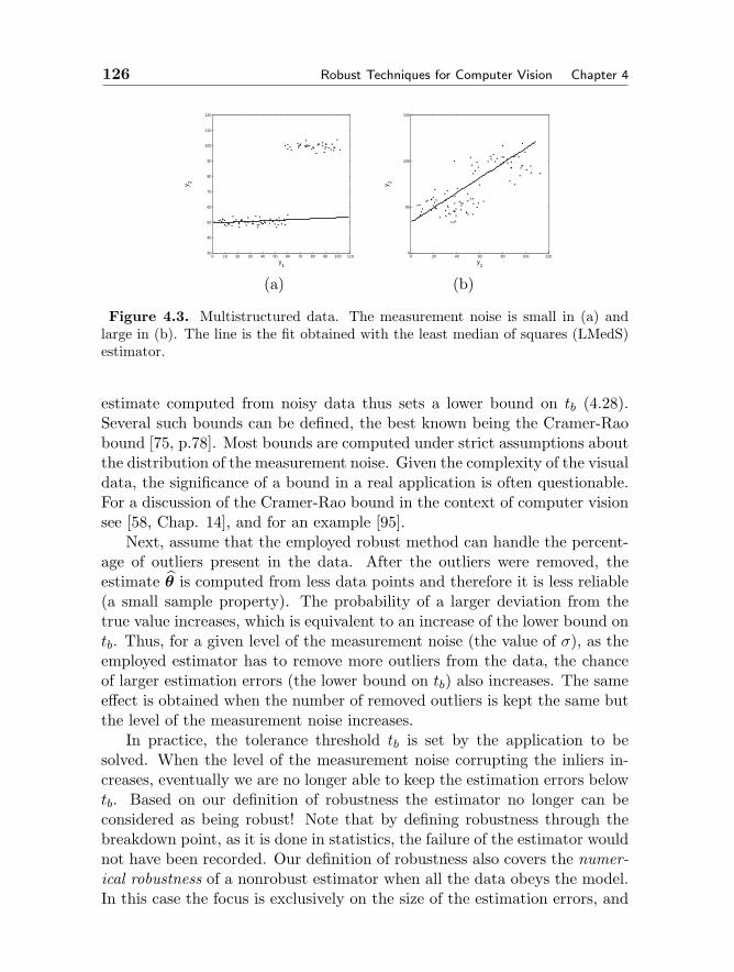
126 Robust Techniques for Computer Vision Chapter 4
0 10 20 30 40 50 60 70 80 90 100 11030
40
50
60
70
80
90
100
110
120
y1
y 2
0 20 40 60 80 100 1200
50
100
150
y1
y 2
(a) (b)
Figure 4.3. Multistructured data. The measurement noise is small in (a) andlarge in (b). The line is the fit obtained with the least median of squares (LMedS)estimator.
estimate computed from noisy data thus sets a lower bound on tb (4.28).Several such bounds can be defined, the best known being the Cramer-Raobound [75, p.78]. Most bounds are computed under strict assumptions aboutthe distribution of the measurement noise. Given the complexity of the visualdata, the significance of a bound in a real application is often questionable.For a discussion of the Cramer-Rao bound in the context of computer visionsee [58, Chap. 14], and for an example [95].
Next, assume that the employed robust method can handle the percent-age of outliers present in the data. After the outliers were removed, theestimate θ is computed from less data points and therefore it is less reliable(a small sample property). The probability of a larger deviation from thetrue value increases, which is equivalent to an increase of the lower bound ontb. Thus, for a given level of the measurement noise (the value of σ), as theemployed estimator has to remove more outliers from the data, the chanceof larger estimation errors (the lower bound on tb) also increases. The sameeffect is obtained when the number of removed outliers is kept the same butthe level of the measurement noise increases.
In practice, the tolerance threshold tb is set by the application to besolved. When the level of the measurement noise corrupting the inliers in-creases, eventually we are no longer able to keep the estimation errors belowtb. Based on our definition of robustness the estimator no longer can beconsidered as being robust! Note that by defining robustness through thebreakdown point, as it is done in statistics, the failure of the estimator wouldnot have been recorded. Our definition of robustness also covers the numer-ical robustness of a nonrobust estimator when all the data obeys the model.In this case the focus is exclusively on the size of the estimation errors, and
Section 4.2. Models and Estimation Problems 127
the property is related to the efficiency of the estimator.The loss of robustness is best illustrated with multistructured data. For
example, the LMedS estimator was designed to reject up to half the pointsbeing outliers. When used to robustly fit a line to the data in Figure 4.3a,correctly recovers the lower structure which contains sixty percent of thepoints. However, when applied to the similar but heavily corrupted datain Figure 4.3b, LMedS completely fails and the obtained fit is not differentfrom that of the nonrobust least squares [9], [77], [97]. As will be shown inSection 4.4.7, the failure of LMedS is part of a more general deficiency ofrobust estimators.
4.2.5 Taxonomy of Estimation Problems
The model described at the beginning of Section 4.2.2, the measurementequation
yi = yio + δyi yi ∈ Rq δyi ∼ GI(0, σ2Cy) i = 1, . . . , n (4.31)
and the constraint
α+ xioθ = 0 xio = x(yio) i = 1, . . . , n (4.32)
is general enough to apply to almost all computer vision problems. Theconstraint is linear in the parameters α and θ, but nonlinear in the variablesyi. A model in which all the variables are measured with errors is called instatistics an errors-in-variables (EIV) model [111], [115].
We have already discussed in Section 4.2.1 the problem of ellipse fittingusing such nonlinear EIV model (Figure 4.1). Nonlinear EIV models alsoappear in any computer vision problem in which the constraint has to cap-ture an incidence relation in projective geometry. For example, consider theepipolar constraint between the affine coordinates of corresponding points intwo images A and B
[yB1o yB2o 1]F [yA1o yA2o 1] = 0 (4.33)
where F is a rank two matrix [43, Chap.8]. When this bilinear constraint isrewritten as (4.32) four of the eight carriers
xo = [yA1o yA2o yB1o yB2o yA1oyB1o yA2oyB1o yA2oyB1o yA2oyB2o]
(4.34)are nonlinear functions in the variables. Several nonlinear EIV models usedin recovering 3D structure from uncalibrated image sequences are discussedin [34].

128 Robust Techniques for Computer Vision Chapter 4
05
1015
20
0
5
10
15
200
5
10
15
y1y2z
Figure 4.4. A typical traditional regression problem. Estimate the parameters ofthe surface defined on a sampling grid.
To obtain an unbiased estimate, the parameters of a nonlinear EIV modelhave to be computed with nonlinear optimization techniques such as theLevenberg-Marquardt method. See [43, Appen.4] for a discussion. However,the estimation problem can be also approached as a linear model in thecarriers and taking into account the heteroscedasticity of the noise processassociated with the carriers (Section 4.2.1). Several such techniques wereproposed in the computer vision literature: the renormalization method [58],the heteroscedastic errors-in-variables (HEIV) estimator [64], [71], [70] andthe fundamental numerical scheme (FNS) [12]. All of them return estimatesunbiased in a first order approximation.
Since the focus of this chapter is on robust estimation, we will only usethe less general, linear errors-in-variables regression model. In this casethe carriers are linear expressions in the variables, and the constraint (4.32)becomes
α+ yioθ = 0 i = 1, . . . , n . (4.35)
An important particular case of the general EIV model is obtained byconsidering the constraint (4.4). This is the traditional regression modelwhere only a single variable, denoted z, is measured with error and thereforethe measurement equation becomes
zi = zio + δzi δzi ∼ GI(0, σ2) i = 1, . . . , n (4.36)yi = yio i = 1, . . . , n
while the constraint is expressed as
zio = α+ xioθ xio = x(yio) i = 1, . . . , n . (4.37)
Note that the nonlinearity of the carriers is no longer relevant in the tradi-tional regression model since now their value is known.
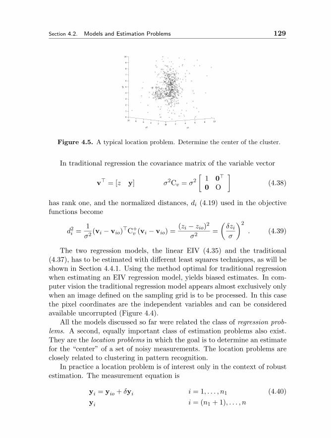
Section 4.2. Models and Estimation Problems 129
0 2 4 6 8 10
0246810
0
1
2
3
4
5
6
7
8
9
10
y1y2
y3
Figure 4.5. A typical location problem. Determine the center of the cluster.
In traditional regression the covariance matrix of the variable vector
v = [z y] σ2Cv = σ2[
1 0
0 O
](4.38)
has rank one, and the normalized distances, di (4.19) used in the objectivefunctions become
d2i =
1σ2 (vi − vio)C+
v (vi − vio) =(zi − zio)2
σ2 =(δziσ
)2
. (4.39)
The two regression models, the linear EIV (4.35) and the traditional(4.37), has to be estimated with different least squares techniques, as will beshown in Section 4.4.1. Using the method optimal for traditional regressionwhen estimating an EIV regression model, yields biased estimates. In com-puter vision the traditional regression model appears almost exclusively onlywhen an image defined on the sampling grid is to be processed. In this casethe pixel coordinates are the independent variables and can be consideredavailable uncorrupted (Figure 4.4).
All the models discussed so far were related the class of regression prob-lems. A second, equally important class of estimation problems also exist.They are the location problems in which the goal is to determine an estimatefor the “center” of a set of noisy measurements. The location problems areclosely related to clustering in pattern recognition.
In practice a location problem is of interest only in the context of robustestimation. The measurement equation is
yi = yio + δyi i = 1, . . . , n1 (4.40)yi i = (n1 + 1), . . . , n
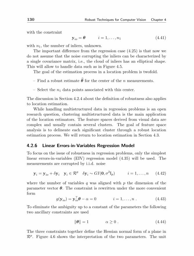
130 Robust Techniques for Computer Vision Chapter 4
with the constraintyio = θ i = 1, . . . , n1 (4.41)
with n1, the number of inliers, unknown.The important difference from the regression case (4.25) is that now we
do not assume that the noise corrupting the inliers can be characterized bya single covariance matrix, i.e., the cloud of inliers has an elliptical shape.This will allow to handle data such as in Figure 4.5.
The goal of the estimation process in a location problem is twofold.
– Find a robust estimate θ for the center of the n measurements.
– Select the n1 data points associated with this center.
The discussion in Section 4.2.4 about the definition of robustness also appliesto location estimation.
While handling multistructured data in regression problems is an openresearch question, clustering multistructured data is the main applicationof the location estimators. The feature spaces derived from visual data arecomplex and usually contain several clusters. The goal of feature spaceanalysis is to delineate each significant cluster through a robust locationestimation process. We will return to location estimation in Section 4.3.
4.2.6 Linear Errors-in-Variables Regression Model
To focus on the issue of robustness in regression problems, only the simplestlinear errors-in-variables (EIV) regression model (4.35) will be used. Themeasurements are corrupted by i.i.d. noise
yi = yio + δyi yi ∈ Rp δyi ∼ GI(0, σ2Ip) i = 1, . . . , n (4.42)
where the number of variables q was aligned with p the dimension of theparameter vector θ. The constraint is rewritten under the more convenientform
g(yio) = yioθ − α = 0 i = 1, . . . , n . (4.43)
To eliminate the ambiguity up to a constant of the parameters the followingtwo ancillary constraints are used
‖θ‖ = 1 α ≥ 0 . (4.44)
The three constraints together define the Hessian normal form of a plane inRp. Figure 4.6 shows the interpretation of the two parameters. The unit
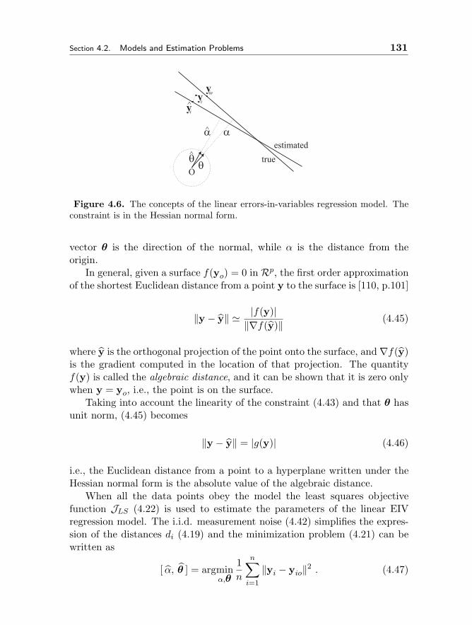
Section 4.2. Models and Estimation Problems 131
Figure 4.6. The concepts of the linear errors-in-variables regression model. Theconstraint is in the Hessian normal form.
vector θ is the direction of the normal, while α is the distance from theorigin.
In general, given a surface f(yo) = 0 in Rp, the first order approximationof the shortest Euclidean distance from a point y to the surface is [110, p.101]
‖y − y‖ |f(y)|‖∇f(y)‖ (4.45)
where y is the orthogonal projection of the point onto the surface, and∇f(y)is the gradient computed in the location of that projection. The quantityf(y) is called the algebraic distance, and it can be shown that it is zero onlywhen y = yo, i.e., the point is on the surface.
Taking into account the linearity of the constraint (4.43) and that θ hasunit norm, (4.45) becomes
‖y − y‖ = |g(y)| (4.46)
i.e., the Euclidean distance from a point to a hyperplane written under theHessian normal form is the absolute value of the algebraic distance.
When all the data points obey the model the least squares objectivefunction JLS (4.22) is used to estimate the parameters of the linear EIVregression model. The i.i.d. measurement noise (4.42) simplifies the expres-sion of the distances di (4.19) and the minimization problem (4.21) can bewritten as
[ α, θ ] = argminα,θ
1n
n∑i=1
‖yi − yio‖2 . (4.47)

132 Robust Techniques for Computer Vision Chapter 4
Combining (4.46) and (4.47) we obtain
[ α, θ ] = argminα,θ
1n
n∑i=1
g(yi)2 . (4.48)
To solve (4.48) the true values yio are replaced with the orthogonal projectionof the yi-s onto the hyperplane. The orthogonal projections yi associatedwith the solution α, θ are the corrected values of the measurements yi, andsatisfy (Figure 4.6)
g(yi) = yi θ − α = 0 i = 1, . . . , n . (4.49)
The estimation process (to be discussed in Section 4.4.1) returns the pa-rameter estimates, after which the ancillary constrains (4.44) can be imposed.The employed parametrization of the linear model
ω1 = [θ α] = [θ1 θ2 · · · θp α] ∈ Rp+1 (4.50)
however is redundant. The vector θ being a unit vector it is restricted tothe p-dimensional unit sphere in Rp. This can be taken into account byexpressing θ in polar angles [115] as, θ = θ(β)
β = [β1 β2 · · · βp−1] 0 ≤ βj ≤ π j = 1, · · · , p− 2 0 ≤ βp−1 < 2π
(4.51)where the mapping is
θ1(β) = sinβ1 · · · sinβp−2 sinβp−1
θ2(β) = sinβ1 · · · sinβp−2 cosβp−1
θ3(β) = sinβ1 · · · sinβp−3 cosβp−2
... (4.52)θp−1(β) = sinβ1 cosβ2
θp(β) = cosβ1 .
The polar angles βj and α provide the second representation of a hyperplane
ω2 = [β α] = [β1 β2 · · · βp−1 α] ∈ Rp . (4.53)
The ω2 representation being based in part on the mapping from the unitsphere to Rp−1, is inherently discontinuos. See [24, Chap. 5] for a detaileddiscussion of such representations. The problem is well known in the contextof Hough transform, where this parametrization is widely used.
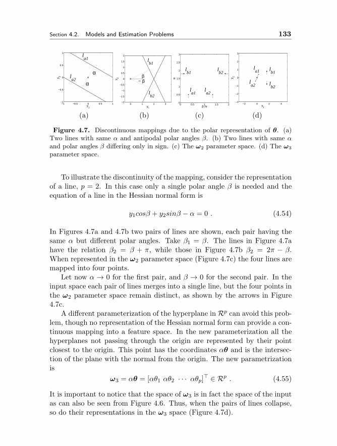
Section 4.2. Models and Estimation Problems 133
−1 −0.5 0 0.5 1−1
−0.5
0
0.5
1
y1
y 2 la2
la1
α
α
0 1 2 3−2
−1.5
−1
−0.5
0
0.5
1
1.5
2
y1
y 2
lb1
lb2
β− β
0 0.5 1 1.5 20
0.5
1
1.5
2
2.5
3
la1
la2
lb1
lb2
β /π
α
−2 0 2 4−3
−2
−1
0
1
2
3
la1
la2
lb1
lb2
y1
y 2
(a) (b) (c) (d)
Figure 4.7. Discontinuous mappings due to the polar representation of θ. (a)Two lines with same α and antipodal polar angles β. (b) Two lines with same αand polar angles β differing only in sign. (c) The ω2 parameter space. (d) The ω3parameter space.
To illustrate the discontinuity of the mapping, consider the representationof a line, p = 2. In this case only a single polar angle β is needed and theequation of a line in the Hessian normal form is
y1cosβ + y2sinβ − α = 0 . (4.54)
In Figures 4.7a and 4.7b two pairs of lines are shown, each pair having thesame α but different polar angles. Take β1 = β. The lines in Figure 4.7ahave the relation β2 = β + π, while those in Figure 4.7b β2 = 2π − β.When represented in the ω2 parameter space (Figure 4.7c) the four lines aremapped into four points.
Let now α → 0 for the first pair, and β → 0 for the second pair. In theinput space each pair of lines merges into a single line, but the four points inthe ω2 parameter space remain distinct, as shown by the arrows in Figure4.7c.
A different parameterization of the hyperplane in Rp can avoid this prob-lem, though no representation of the Hessian normal form can provide a con-tinuous mapping into a feature space. In the new parameterization all thehyperplanes not passing through the origin are represented by their pointclosest to the origin. This point has the coordinates αθ and is the intersec-tion of the plane with the normal from the origin. The new parametrizationis
ω3 = αθ = [αθ1 αθ2 · · · αθp] ∈ Rp . (4.55)
It is important to notice that the space of ω3 is in fact the space of the inputas can also be seen from Figure 4.6. Thus, when the pairs of lines collapse,so do their representations in the ω3 space (Figure 4.7d).
134 Robust Techniques for Computer Vision Chapter 4
Planes which contain the origin have to be treated separately. In practicethis also applies to planes passing near the origin. A plane with small α istranslated along the direction of the normal θ with a known quantity τ .The plane is then represented as τθ. When m planes are close to the origin
the direction of translation ism∑i=1
θi and the parameters of each translated
plane are adjusted accordingly. After processing in the ω3 space it is easyto convert back to the ω1 representation.
Estimation of the linear EIV regression model parameters by total leastsquares (Section 4.4.1) uses the ω1 parametrization. The ω2 parametrizationwill be employed in the robust estimation of the model (Section 4.4.5). Theparametrization ω3 is useful when the problem of robust multiple regressionis approached as a feature space analysis problem [9].
4.2.7 Objective Function Optimization
The objective functions used in robust estimation are often nondifferentiableand analytical optimization methods, like those based on the gradient, can-not be employed. The k-th order statistics, JLkOS (4.22) is such an ob-jective function. Nondifferentiable objective functions also have many localextrema and to avoid being trapped in one of these minima the optimizationprocedure should be run starting from several initial positions. A numericaltechnique to implement robust estimators with nondifferentiable objectivefunctions, is based on elemental subsets.
An elemental subset is the smallest number of data points required tofully instantiate a model. In the linear EIV regression case this means ppoints in a general position, i.e., the points define a basis for a (p − 1)-dimensional affine subspace in Rp [89, p. 257]. For example, if p = 3 not allthree points can lie on a line in 3D.
The p points in an elemental subset thus define a full rank system ofequations from which the model parameters α and θ can be computed ana-lytically. Note that using p points suffices to solve this homogeneous system.The ancillary constraint ‖θ‖ = 1 is imposed at the end. The obtained pa-rameter vector ω1 = [θ α] will be called, with a slight abuse of notation,a model candidate.
The number of possibly distinct elemental subsets in the data(np
), can
be very large. In practice an exhaustive search over all the elemental subsetsis not feasible, and a random sampling of this ensemble has to be used.The sampling drastically reduces the amount of computations at the priceof a negligible decrease in the outlier rejection capability of the implemented
Section 4.2. Models and Estimation Problems 135
robust estimator.Assume that the number of inliers in the data is n1, and that N elemental
subsets, p-tuples, were drawn independently from that data. The probabilitythat none of these subsets contains only inliers is (after disregarding theartifacts due to the finite sample size)
Pfail =[1−
(n1
n
)p]N. (4.56)
We can choose a small probability Perror to bound upward Pfail. Then theequation
Pfail = Perror (4.57)
provides the value of N as a function of the percentage of inliers n1/n, thedimension of the parameter space p and Perror. This probabilistic samplingstrategy was applied independently in computer vision for the RANSACestimator [26] and in statistics for the LMedS estimator [89, p.198].
Several important observations has to be made. The value of N obtainedfrom (4.57) is an absolute lower bound since it implies that any elementalsubset which contains only inliers can provide a satisfactory model candidate.However, the model candidates are computed from the smallest possiblenumber of data points and the influence of the noise is the largest possible.Thus, the assumption used to compute N is not guaranteed to be satisfiedonce the measurement noise becomes significant. In practice n1 is not knowprior to the estimation, and the value of N has to be chosen large enough tocompensate for the inlier noise under a worst case scenario.
Nevertheless, it is not recommended to increase the size of the subsets.The reason is immediately revealed if we define in a drawing of subsets ofsize q ≥ p, the probability of success as obtaining a subset which containsonly inliers
Psuccess =
(n1q
)(nq
) =q−1∏k=0
n1 − kn− k . (4.58)
This probability is maximized when q = p.Optimization of an objective function using random elemental subsets
is only a computational tool and has no bearing on the robustness of thecorresponding estimator. This fact is not always recognized in the computervision literature. However, any estimator can be implemented using the fol-lowing numerical optimization procedure.
136 Robust Techniques for Computer Vision Chapter 4
Objective Function Optimization With Elemental Subsets
– Repeat N times:1. choose an elemental subset (p-tuple) by random sampling;
2. compute the corresponding model candidate;
3. compute the value of the objective function by assuming the modelcandidate valid for all the data points.
– The parameter estimate is the model candidate yielding the smallest(largest) objective function value.
This procedure can be applied the same way for the nonrobust least squaresobjective function JLS as for the the robust least k-th order statistics JLkOS(4.22). However, while an analytical solution is available for the former(Section 4.4.1), for the latter the above procedure is the only practical wayto obtain the estimates.
Performing an exhaustive search over all elemental subsets does not guar-antee to find the global extremum of the objective function since not everylocation in the parameter space can be visited. Finding the global extremum,however, most often is also not required. When a robust estimator is im-plemented with the elemental subsets based search procedure, the goal isonly to obtain the inlier/outlier dichotomy, i.e., to select the “good” data.The robust estimate corresponding to an elemental subset is then refined byprocessing the selected inliers with a nonrobust (least squares) estimator.See [87] for an extensive discussion of the related issues from a statisticalperspective.
The number of required elemental subsets N can be significantly reducedwhen information about the reliability of the data points is available. Thisinformation can be either provided by the user, or can be derived from thedata through an auxiliary estimation process. The elemental subsets arethen chosen with a guided sampling biased toward the points having a higherprobability to be inliers. See [103] and [104] for computer vision examples.
We have emphasized that the random sampling of elemental subsets isnot more than a computational procedure. However, guided sampling hasa different nature since it relies on a fuzzy pre-classification of the data(derived automatically, or supplied by the user). Guided sampling can yielda significant improvement in the performance of the estimator relative tothe unguided approach. The better quality of the elemental subsets canbe converted into either less samples in the numerical optimization (whilepreserving the outlier rejection capacity η(n) of the estimator), or into anincrease of η(n) (while preserving the same number of elemental subsets N).
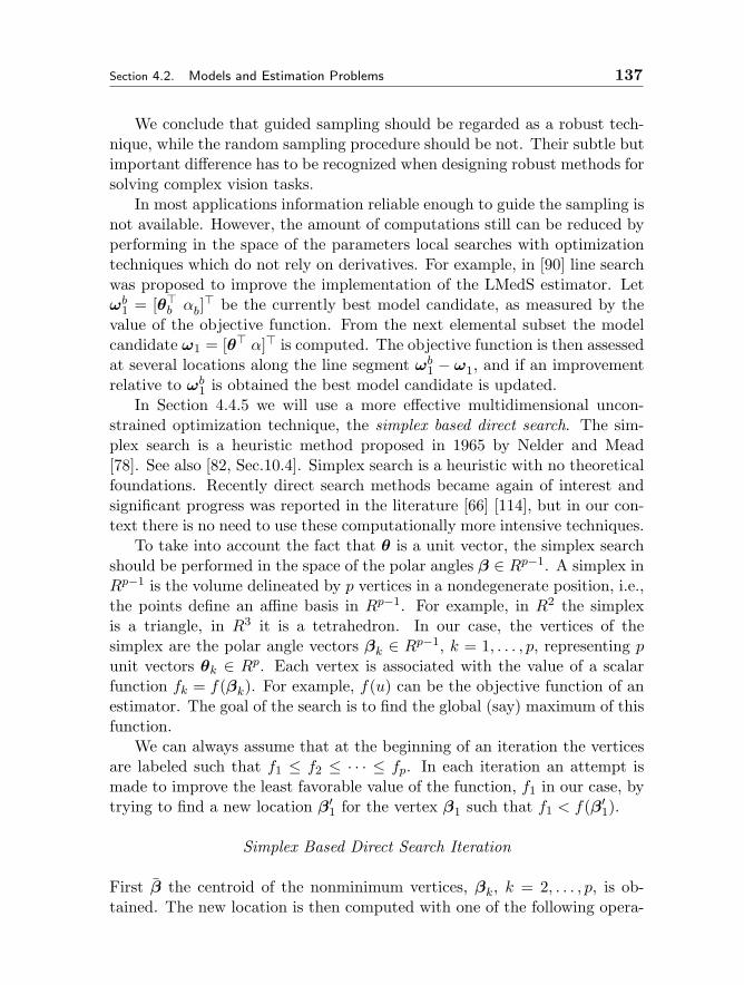
Section 4.2. Models and Estimation Problems 137
We conclude that guided sampling should be regarded as a robust tech-nique, while the random sampling procedure should be not. Their subtle butimportant difference has to be recognized when designing robust methods forsolving complex vision tasks.
In most applications information reliable enough to guide the sampling isnot available. However, the amount of computations still can be reduced byperforming in the space of the parameters local searches with optimizationtechniques which do not rely on derivatives. For example, in [90] line searchwas proposed to improve the implementation of the LMedS estimator. Letωb
1 = [θb αb]
be the currently best model candidate, as measured by thevalue of the objective function. From the next elemental subset the modelcandidate ω1 = [θ α] is computed. The objective function is then assessedat several locations along the line segment ωb
1 − ω1, and if an improvementrelative to ωb
1 is obtained the best model candidate is updated.In Section 4.4.5 we will use a more effective multidimensional uncon-
strained optimization technique, the simplex based direct search. The sim-plex search is a heuristic method proposed in 1965 by Nelder and Mead[78]. See also [82, Sec.10.4]. Simplex search is a heuristic with no theoreticalfoundations. Recently direct search methods became again of interest andsignificant progress was reported in the literature [66] [114], but in our con-text there is no need to use these computationally more intensive techniques.
To take into account the fact that θ is a unit vector, the simplex searchshould be performed in the space of the polar angles β ∈ Rp−1. A simplex inRp−1 is the volume delineated by p vertices in a nondegenerate position, i.e.,the points define an affine basis in Rp−1. For example, in R2 the simplexis a triangle, in R3 it is a tetrahedron. In our case, the vertices of thesimplex are the polar angle vectors βk ∈ Rp−1, k = 1, . . . , p, representing punit vectors θk ∈ Rp. Each vertex is associated with the value of a scalarfunction fk = f(βk). For example, f(u) can be the objective function of anestimator. The goal of the search is to find the global (say) maximum of thisfunction.
We can always assume that at the beginning of an iteration the verticesare labeled such that f1 ≤ f2 ≤ · · · ≤ fp. In each iteration an attempt ismade to improve the least favorable value of the function, f1 in our case, bytrying to find a new location β′
1 for the vertex β1 such that f1 < f(β′1).
Simplex Based Direct Search Iteration
First β the centroid of the nonminimum vertices, βk, k = 2, . . . , p, is ob-tained. The new location is then computed with one of the following opera-
138 Robust Techniques for Computer Vision Chapter 4
1 1.5 2 2.50
0.5
1
1.5
2
2.5
β1
β 2β
1
β2
β3
β−
β1’
1 1.5 2 2.50
0.5
1
1.5
2
2.5
β1
β 2β
1
β2
β3
β−
β1’
1 1.5 2 2.50
0.5
1
1.5
2
2.5
β1
β 2β
1
β2
β3
β−
β1’
1 1.5 2 2.50
0.5
1
1.5
2
2.5
β1
β 2β
1
β2
β3
β−
β’1
1 1.5 2 2.50
0.5
1
1.5
2
2.5
β1
β 2β
1
β2
β3
β−
β’1
1 1.5 2 2.50
0.5
1
1.5
2
2.5
β1
β 2β
1
β2
β3
β−
β’1
1 1.5 2 2.50
0.5
1
1.5
2
2.5
β1
β 2β
1
β2
β3
β−
β’1
1 1.5 2 2.50
0.5
1
1.5
2
2.5
β1
β 2β
1
β2
β3
β−
β’1
1 1.5 2 2.50
0.5
1
1.5
2
2.5
β1
β 2β
1
β2
β3
β−
β’1
1 1.5 2 2.50
0.5
1
1.5
2
2.5
β1
β 2β
1
β2
β3
β−
β’1
1 1.5 2 2.50
0.5
1
1.5
2
2.5
β1
β 2β
1
β2
β3
β−
β’1
1 1.5 2 2.50
0.5
1
1.5
2
2.5
β1
β 2β
1
β2
β3
β−
β1’
1 1.5 2 2.50
0.5
1
1.5
2
2.5
β1
β 2
β1
β2
β3
β−
β1’
1 1.5 2 2.50
0.5
1
1.5
2
2.5
β1
β 2
β1
β2
β3
β−
β1’
1 1.5 2 2.50
0.5
1
1.5
2
2.5
β1
β 2
β1
β2
β3
β−
β1’
1 1.5 2 2.50
0.5
1
1.5
2
2.5
β1
β 2
β1
β2
β3
β−
β’1
1 1.5 2 2.50
0.5
1
1.5
2
2.5
β1
β 2
β1
β2
β3
β−
β’1
1 1.5 2 2.50
0.5
1
1.5
2
2.5
β1
β 2
β1
β2
β3
β−
β’1
1 1.5 2 2.50
0.5
1
1.5
2
2.5
β1
β 2
β1
β2
β3
β−
β’1
1 1.5 2 2.50
0.5
1
1.5
2
2.5
β1
β 2
β1
β2
β3
β−
β’1
1 1.5 2 2.50
0.5
1
1.5
2
2.5
β1
β 2
β1
β2
β3
β−
β’1
1 1.5 2 2.50
0.5
1
1.5
2
2.5
β1
β 2
β1
β2
β3
β−
β’1
1 1.5 2 2.50
0.5
1
1.5
2
2.5
β1
β 2
β1
β2
β3
β−
β’1
1 1.5 2 2.50
0.5
1
1.5
2
2.5
β1
β 2
β1
β2
β3
β−
β1’
1 1.5 2 2.50
0.5
1
1.5
2
2.5
β1
β 2
β1
β2
β3
β−
β1’
1 1.5 2 2.50
0.5
1
1.5
2
2.5
β1
β 2
β1
β2
β3
β−
β1’
1 1.5 2 2.50
0.5
1
1.5
2
2.5
β1
β 2
β1
β2
β3
β−
β’1
1 1.5 2 2.50
0.5
1
1.5
2
2.5
β1
β 2
β1
β2
β3
β−
β’1
1 1.5 2 2.50
0.5
1
1.5
2
2.5
β1
β 2
β1
β2
β3
β−
β’1
1 1.5 2 2.50
0.5
1
1.5
2
2.5
β1
β 2
β1
β2
β3
β−
β’1
1 1.5 2 2.50
0.5
1
1.5
2
2.5
β1
β 2
β1
β2
β3
β−
β’1
1 1.5 2 2.50
0.5
1
1.5
2
2.5
β1
β 2
β1
β2
β3
β−
β’1
1 1.5 2 2.50
0.5
1
1.5
2
2.5
β1
β 2
β1
β2
β3
β−
β1’
1 1.5 2 2.50
0.5
1
1.5
2
2.5
β1
β 2
β1
β2
β3
β−
β1’
1 1.5 2 2.50
0.5
1
1.5
2
2.5
β1
β 2
β1
β2
β3
β−
β1’
1 1.5 2 2.50
0.5
1
1.5
2
2.5
β1
β 2
β1
β2
β3
β−
β’1
1 1.5 2 2.50
0.5
1
1.5
2
2.5
β1
β 2
β1
β2
β3
β−
β’1
1 1.5 2 2.50
0.5
1
1.5
2
2.5
β1
β 2
β1
β2
β3
β−
β’1
1 1.5 2 2.50
0.5
1
1.5
2
2.5
β1
β 2
β1
β2
β3
β−
β’1
1 1.5 2 2.50
0.5
1
1.5
2
2.5
β1
β 2
β1
β2
β3
β−
β’1
1 1.5 2 2.50
0.5
1
1.5
2
2.5
β1
β 2
β1
β2
β3
β−
β’1
1 1.5 2 2.50
0.5
1
1.5
2
2.5
β1
β 2
β1
β2
β3
β−
β’1
(a) (b) (c) (d)
Figure 4.8. Basic operations in simplex based direct search. (a) Reflection. (b)Expansion. (c) Outside contraction. (d) Inside contraction.
tions along the direction β − β1: reflection, expansion and contraction.
1. The reflection of β1, denoted β′ (Figure 4.8a) is defined as
β′ = crβ1 + (1− cr)β (4.59)
where cr < 0 is the reflection coefficient. If f2 < f(β′) ≤ fp, thenβ′
1 = β′ and the next iteration is started.
2. If f(β′) > fp, i.e., the reflection has produced a new maximum, thesimplex is expanded by moving β′ to β∗ (Figure 4.8b)
β∗ = ceβ′ + (1− ce)β (4.60)
where the expansion coefficient ce > 1. If f(β∗) > f(β′) the expansionis successful and β′
1 = β∗. Else, β′1 = β′. The next iteration is started.
3. If f(β′) ≤ f2, the vector β1n is defined as either β1 or β′, whicheverhas the larger associated function value, and a contraction is performed
β∗ = ccβ1n + (1− cc)β . (4.61)
First, a contraction coefficient 0 < cc < 1 is chosen for outside contrac-tion (Figure 4.8c). If f(β∗) > f(β1n), then β′
1 = β∗ and the nextiteration is started. Otherwise, an inside contraction is performed(Figure 4.8d) in which cc is replaced with −cc, and the conditionf(β∗) > f(β1n) is again verified.
4. Should both contractions fail all the vertices are updated
βk ←−12(βk + βp
)k = 1, . . . , (p− 1) (4.62)
and the next iteration is started.

Section 4.3. Location Estimation 139
020
4060
80
0
20
40
60
80
0
20
40
60
80
y1
y2
y 3
2040
6080
100
0
20
40
60
80
100
−50
0
50
L*
u*
v*
(a) (b)
Figure 4.9. Multistructured data in the location estimation problem. (a) The“traditional” case. (b) A typical computer vision example.
Recommended values for the coefficients are cr = −1, ce = 1.5, cc = 0.5.
To assess the convergence of the search several stopping criteria can be em-ployed. For example, the variance of the p function values fk should fallbelow a threshold which is exponentially decreasing with the dimension ofthe space, or the ratio of the smallest and largest function values f1/fp shouldbe close to one. Similarly, the volume of the simplex should shrink belowa dimension dependent threshold. In practice, the most effective stoppingcriteria are application specific incorporating additional information whichwas not used during the optimization.
In the previous sections we have analyzed the problem of robust estima-tion from a generic point of view. We can proceed now to examine the twoclasses of estimation problems: location and regression. In each case willintroduce a new robust technique whose improved behavior was achieved bysystematically exploiting the principles discussed so far.
4.3 Location Estimation
In this section will show that in the context of computer vision tasks oftenonly nonparametric approaches can provide a robust solution for the locationestimation problem. We employ a class of nonparametric techniques in whichthe data points are regarded as samples from an unknown probability density.The location estimates are then defined as the modes of this density. Explicitcomputation of the density is avoided by using the mean shift procedure.
140 Robust Techniques for Computer Vision Chapter 4
4.3.1 Why Nonparametric Methods
The most general model of the location problem is that of multiple structures
k = 1, . . . ,K m1 = 1 · · · mK+1 = n1 + 1
y(k)i = y(k)
io + δyi y(k)io = θ(k) i = mk, . . . , (mk+1 − 1)
yi i = (n1 + 1), . . . , n (4.63)
with no information being available about the nature of the inlier noise δyi,the n− n1 outliers, or the number of structures present in the data K. Themodel (4.63) is also used in cluster analysis, the equivalent pattern recog-nition problem. Clustering under its most general form is an unsupervisedlearning method of unknown categories from incomplete prior information[52, p. 242]. The books [52], [21, Chap. 10], [44, Sec.14.3] provide a completecoverage of the related pattern recognition literature.
Many of the pattern recognition methods are not adequate for data anal-ysis in computer vision. To illustrate their limitations will compare the twodata sets shown in Figure 4.9. The data in Figure 4.9a obeys what is assumedin traditional clustering methods when the proximity to a cluster center ismeasured as a function of Euclidean or Mahalanobis distances. In this casethe shape of the clusters is restricted to elliptical and the inliers are assumedto be normally distributed around the true cluster centers. A different metricwill impose a different shape on the clusters. The number of the structures(clusters) K, is a parameter to be supplied by the user and has a large influ-ence on the quality of the results. While the value of K can be also derivedfrom the data by optimizing a cluster validity index, this approach is notrobust since it is based on (possibly erroneous) data partitions.
Expectation maximization (EM) is a frequently used technique today incomputer vision to model the data. See [44, Sec.8.5.2] for a short description.The EM algorithm also relies on strong prior assumptions. A likelihood func-tion, defined from a mixture of predefined (most often normal) probabilitydensities, is maximized. The obtained partition of the data thus employs“tiles” of given shape. The number of required mixture components is oftendifficult to determine, and the association of these components with truecluster centers may not be obvious.
Examine now the data in Figure 4.9b in which the pixels of a colorimage were mapped into the three-dimensional L∗u∗v∗ color space. Thesignificant clusters correspond to similarly colored pixels in the image. Theclusters have a large variety of shapes and their number is not obvious. Anytechnique which imposes a preset shape on the clusters will have difficulties

Section 4.3. Location Estimation 141
to accurately separate K significant structures from the background clutterwhile simultaneously also having to determine the value of K.
Following our goal oriented approach toward robustness (Section 4.2.3) alocation estimator should be declared robust only if it returns a satisfactoryresult. From the above discussion can be concluded that robustly solvinglocation problems in computer vision often requires techniques which use theleast possible amount of prior assumptions about the data. Such techniquesbelong to the family of nonparametric methods.
In nonparametric methods the n data points are regarded as outcomesfrom an (unknown) probability distribution f(y). Each data point is as-sumed to have an equal probability
Prob[y = yi] =1n
i = 1, . . . , n . (4.64)
When several points have the same value, the probability is n−1 timesthe multiplicity. The ensemble of points defines the empirical distributionf(y|y1 · · ·yn) of the data. The empirical distribution is the nonparametricmaximum likelihood estimate of the distribution from which the data wasdrawn [22, p.310]. It is also the “least committed” description of the data.
Every clustering technique exploits the fact that the clusters are thedenser regions in the space. However, this observation can be pushed furtherin the class of nonparametric methods considered here, for which a regionof higher density implies more probable outcomes of the random variable y.Therefore, in each dense region the location estimate (cluster center) shouldbe associated with the most probable value of y, i.e., with the local mode ofthe empirical distribution
θ(k)
= argmaxy k f(y|y1 · · ·yn) k = 1, . . . ,K . (4.65)
Note that by detecting all the significant modes of the empirical distributionthe number of clusters K is automatically determined. The mode basedclustering techniques make extensive use of density estimation during dataanalysis.
4.3.2 Kernel Density Estimation
The modes of a random variable y are the local maxima of its probabilitydensity function f(y). However, only the empirical distribution, the datapoints yi, i = 1, . . . , n are available. To accurately determine the locationsof the modes, first a continuous estimate of the underlying density f(y) has

142 Robust Techniques for Computer Vision Chapter 4
to be defined. Later we will see that this step can be eliminated by directlyestimating the gradient of the density (Section 4.3.3).
To estimate the probability density in y a small neighborhood is definedaround y. The neighborhood usually has a simple shape: cube, sphere orellipsoid. Let its volume be Vy, and my be the number of data points inside.Then the density estimate is [21, Sec.4.2]
f(y) =my
nVy(4.66)
which can be employed in two different ways.– In the nearest neighbors approach, the neigborhoods (the volumes Vy)
are scaled to keep the number of points my constant. A mode cor-responds to a location in which the neighborhood has the smallestvolume.
– In the kernel density approach, the neigborhoods have the same volumeVy and the number of points my inside are counted. A mode corre-sponds to a location in which the neighborhood contains the largestnumber of points.
The minimum volume ellipsoid (MVE) robust location estimator pro-posed in statistics [89, p.258], is a technique related to the nearest neighborsapproach. The ellipsoids are defined by elemental subsets obtained throughrandom sampling, and the numerical optimization procedure discussed inSection 4.2.7 is employed. The location estimate is the center of the smallestellipsoid which contains a given percentage of the data points. In a robustclustering method proposed in computer vision the MVE estimator was usedto sequentially remove the clusters from the data, starting from the largest[53]. However, by imposing an elliptical shape for the clusters severe ar-tifacts were introduced and the method was never successful in real visionapplications.
For our goal of finding the local maxima of f(y), the kernel density meth-ods are more suitable. Kernel density estimation is a widely used techniquein statistics and pattern recognition, where it is also called the Parzen win-dow method. See [92], [112] for a description in statistics, and [21, Sec.4.3][44, Sec. 6.6] for a description in pattern recognition.
Will start with the simplest case of one-dimensional data. Let yi, i =1, . . . , n, be scalar measurements drawn from an arbitrary probability distri-bution f(y). The kernel density estimate f(y) of this distribution is obtained
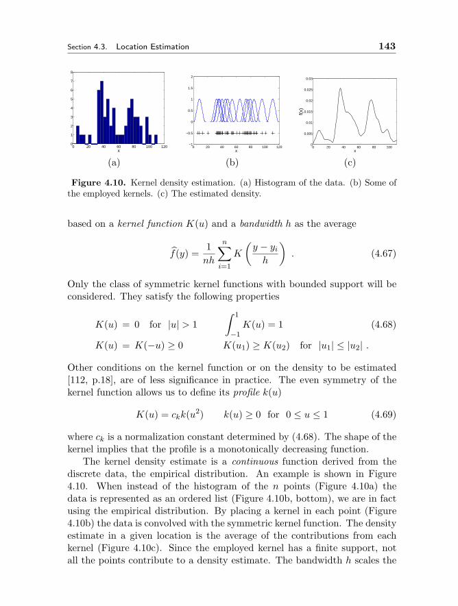
Section 4.3. Location Estimation 143
0 20 40 60 80 100 1200
1
2
3
4
5
6
7
8
x0 20 40 60 80 100 120
−1
−0.5
0
0.5
1
1.5
2
x0 20 40 60 80 100
0
0.005
0.01
0.015
0.02
0.025
0.03
x
f(x)
(a) (b) (c)
Figure 4.10. Kernel density estimation. (a) Histogram of the data. (b) Some ofthe employed kernels. (c) The estimated density.
based on a kernel function K(u) and a bandwidth h as the average
f(y) =1nh
n∑i=1
K
(y − yih
). (4.67)
Only the class of symmetric kernel functions with bounded support will beconsidered. They satisfy the following properties
K(u) = 0 for |u| > 1∫ 1
−1K(u) = 1 (4.68)
K(u) = K(−u) ≥ 0 K(u1) ≥ K(u2) for |u1| ≤ |u2| .
Other conditions on the kernel function or on the density to be estimated[112, p.18], are of less significance in practice. The even symmetry of thekernel function allows us to define its profile k(u)
K(u) = ckk(u2) k(u) ≥ 0 for 0 ≤ u ≤ 1 (4.69)
where ck is a normalization constant determined by (4.68). The shape of thekernel implies that the profile is a monotonically decreasing function.
The kernel density estimate is a continuous function derived from thediscrete data, the empirical distribution. An example is shown in Figure4.10. When instead of the histogram of the n points (Figure 4.10a) thedata is represented as an ordered list (Figure 4.10b, bottom), we are in factusing the empirical distribution. By placing a kernel in each point (Figure4.10b) the data is convolved with the symmetric kernel function. The densityestimate in a given location is the average of the contributions from eachkernel (Figure 4.10c). Since the employed kernel has a finite support, notall the points contribute to a density estimate. The bandwidth h scales the
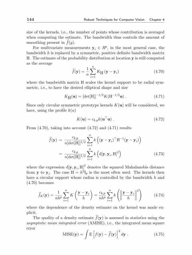
144 Robust Techniques for Computer Vision Chapter 4
size of the kernels, i.e., the number of points whose contribution is averagedwhen computing the estimate. The bandwidth thus controls the amount ofsmoothing present in f(y).
For multivariate measurements yi ∈ Rp, in the most general case, thebandwidth h is replaced by a symmetric, positive definite bandwidth matrixH. The estimate of the probability distribution at location y is still computedas the average
f(y) =1n
n∑i=1
KH (y − yi) (4.70)
where the bandwidth matrix H scales the kernel support to be radial sym-metric, i.e., to have the desired elliptical shape and size
KH(u) = [det[H]]−1/2K(H−1/2u) . (4.71)
Since only circular symmetric prototype kernels K(u) will be considered, wehave, using the profile k(u)
K(u) = ck,pk(uu) . (4.72)
From (4.70), taking into account (4.72) and (4.71) results
f(y) =ck,p
n[det[H]]1/2
n∑i=1
k((y − yi)
H−1(y − yi))
=ck,p
n[det[H]]1/2
n∑i=1
k(d[y,yi,H]2
)(4.73)
where the expression d[y,yi,H]2 denotes the squared Mahalanobis distancefrom y to yi. The case H = h2Ip is the most often used. The kernels thenhave a circular support whose radius is controlled by the bandwidth h and(4.70) becomes
fK(y) =1nhp
n∑i=1
K
(y − yih
)=ck,pnhp
n∑i=1
k
(∥∥∥∥y − yih
∥∥∥∥2)
(4.74)
where the dependence of the density estimate on the kernel was made ex-plicit.
The quality of a density estimate f(y) is assessed in statistics using theasymptotic mean integrated error (AMISE), i.e., the integrated mean squareerror
MISE(y) =∫
E[f(y)− f(y)
]2dy . (4.75)

Section 4.3. Location Estimation 145
between the true density and its estimate for n → ∞ while h → 0 at aslower rate. The expectation is taken over all data sets of size n. Since thebandwidth h of a circular symmetric kernel has a strong influence on thequality of f(y), the bandwidth minimizing an approximation of the AMISEerror is of interest. Unfortunately, this bandwidth depends on f(y), theunknown density [112, Sec.4.3].
For the univariate case several practical rules are available [112, Sec.3.2].For example, the information about f(y) is substituted with σ, a robust scaleestimate derived from the data
h =[
243R(K)35µ2(K)2n
]1/5
σ (4.76)
where
µ2(K) =∫ 1
−1u2K(u)du R(K) =
∫ 1
−1K(u)2du (4.77)
The scale estimate σ will be discussed in Section 4.4.3.For a given bandwidth the AMISE measure is minimized by the Epanech-
nikov kernel [112, p.104] having the profile
kE(u) =
1− u 0 ≤ u ≤ 10 u > 1
(4.78)
which yields the kernel
KE(y) = 1
2c−1p (p+ 2)(1− ‖y‖2) ‖y‖ ≤ 1
0 otherwise(4.79)
where cp is the volume of the p-dimensional unit sphere. Other kernels canalso be defined. The truncated normal has the profile
kN (u) =e−au 0 ≤ u ≤ 1
0 u > 1(4.80)
where a is chosen such that e−a is already negligible small. Neither of the twoprofiles defined above have continuous derivatives at the boundary u = 1.This condition is satisfied (for the first two derivatives) by the biweight kernelhaving the profile
kB(u) =
(1− u)3 0 ≤ u ≤ 10 u > 1
(4.81)
Its name here is taken from robust statistics, in the kernel density estimationliterature it is called the triweight kernel [112, p.31].
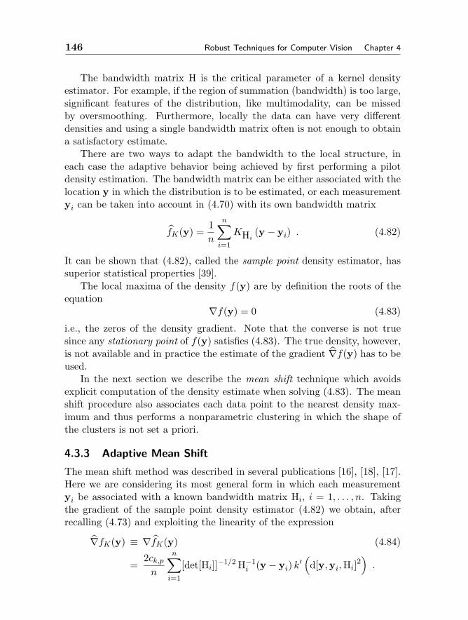
146 Robust Techniques for Computer Vision Chapter 4
The bandwidth matrix H is the critical parameter of a kernel densityestimator. For example, if the region of summation (bandwidth) is too large,significant features of the distribution, like multimodality, can be missedby oversmoothing. Furthermore, locally the data can have very differentdensities and using a single bandwidth matrix often is not enough to obtaina satisfactory estimate.
There are two ways to adapt the bandwidth to the local structure, ineach case the adaptive behavior being achieved by first performing a pilotdensity estimation. The bandwidth matrix can be either associated with thelocation y in which the distribution is to be estimated, or each measurementyi can be taken into account in (4.70) with its own bandwidth matrix
fK(y) =1n
n∑i=1
KHi(y − yi) . (4.82)
It can be shown that (4.82), called the sample point density estimator, hassuperior statistical properties [39].
The local maxima of the density f(y) are by definition the roots of theequation
∇f(y) = 0 (4.83)
i.e., the zeros of the density gradient. Note that the converse is not truesince any stationary point of f(y) satisfies (4.83). The true density, however,is not available and in practice the estimate of the gradient ∇f(y) has to beused.
In the next section we describe the mean shift technique which avoidsexplicit computation of the density estimate when solving (4.83). The meanshift procedure also associates each data point to the nearest density max-imum and thus performs a nonparametric clustering in which the shape ofthe clusters is not set a priori.
4.3.3 Adaptive Mean Shift
The mean shift method was described in several publications [16], [18], [17].Here we are considering its most general form in which each measurementyi be associated with a known bandwidth matrix Hi, i = 1, . . . , n. Takingthe gradient of the sample point density estimator (4.82) we obtain, afterrecalling (4.73) and exploiting the linearity of the expression
∇fK(y) ≡ ∇fK(y) (4.84)
=2ck,pn
n∑i=1
[det[Hi]]−1/2 H−1i (y − yi) k
′(d[y,yi,Hi]
2).

Section 4.3. Location Estimation 147
The function g(x) = −k′(x) satisfies the properties of a profile, and thus wecan define the kernel G(u) = cg,pg(uu). For example, for the Epanechnikovkernel the corresponding new profile is
gE(u) =
1 0 ≤ u ≤ 10 u > 1
(4.85)
and thus GE(u) is the uniform kernel. For convenience will introduce thenotation
Qi(y) = det[Hi]−1/2 H−1i g
(d[y,yi,Hi]
2). (4.86)
From the definition of g(u) and (4.69)
Qi(y) = O d[y,yi,Hi] > 1 . (4.87)
Then (4.84) can be written as
∇fK(y) =2ck,pn
(n∑i=1
Qi(y)
)( n∑i=1
Qi(y)
)−1 n∑i=1
Qi(y)yi − y
(4.88)
and the roots of the equation (4.83) are the solutions of
y =
(n∑i=1
Qi(y)
)−1 n∑i=1
Qi(y)yi (4.89)
which can be solved only iteratively
y[l+1] =
(n∑i=1
Qi
(y[l]))−1 n∑
i=1
Qi
(y[l])yi l = 0, 1, . . . (4.90)
The meaning of an iteration becomes apparent if we consider the particularcase Hi = h2
i I yielding
y =
∑ni=1 yi h
−(p+2)i g
(∥∥∥y−yi
hi
∥∥∥2)
∑ni=1 h
−(p+2)i g
(∥∥∥y−yi
hi
∥∥∥2) (4.91)
and which becomes when all hi = h
y =
∑ni=1 yi g
(∥∥∥y−yi
h
∥∥∥2)
∑ni=1 g
(∥∥∥y−yi
h
∥∥∥2) . (4.92)

148 Robust Techniques for Computer Vision Chapter 4
From (4.87) we see that at every step only a local weighted mean is computed.The robustness of the mode detection method is the direct consequence ofthis property. In the next iteration the computation is repeated centeredon the previously computed mean. The difference between the current andprevious locations, the vector
m[l+1]G = y[l+1] − y[l] l = 0, 1, . . . (4.93)
is called the mean shift vector, where the fact that the weighted averages arecomputed with the kernel G was made explicit. Adapting (4.88) to the twoparticular cases above it can be shown that
m[l+1]G = c
∇fK(y[l])
fG(y[l])(4.94)
where c is a positive constant. Thus, the mean shift vector is aligned with thegradient estimate of the density, and the window of computations is alwaysmoved toward regions of higher density. See [17] for the details. A relationsimilar to (4.94) still holds in the general case, but now the mean shift andgradient vectors are connected by a linear transformation.
In the mean shift procedure the user controls the resolution of the dataanalysis by providing the bandwidth information. Since most often circularsymmetric kernels are used, only the bandwith parameters hi are needed.
Mean Shift Procedure1. Choose a data point yi as the initial y[0].
2. Compute y[l+1], l = 0, 1, . . . the weighted mean of the points at lessthan unit Mahalanobis distance from y[l]. Each point is consideredwith its own metric.
3. Verify if∥∥∥m[l+1]
G
∥∥∥ is less than the tolerance. If yes, stop.
4. Replace y[l] with y[l+1], i.e., move the processing toward a region withhigher point density. Return to Step 2.
The most important properties of the mean shift procedure are illustratedgraphically in Figure 4.11. In Figure 4.11a the setup of the weighted meancomputation in the general case is shown. The kernel associated with a datapoint is nonzero only within the elliptical region centered on that point.
Section 4.3. Location Estimation 149
200 300 400 500 600 700 800200
300
400
500
600
700
800
y
y1
y 2
200 300 400 500 600 700 800200
300
400
500
600
700
800
y
y1
y 2
(a) (b) (c)
Figure 4.11. The main steps in mean shift based clustering. (a) Computation ofthe weighted mean in the general case. (b) Mean shift trajectories of two points ina bimodal data. (c) Basins of attraction.
Thus, only those points contribute to the weighted mean in y whose kernelsupport contains y.
The evolution of the iterative procedure is shown in Figure 4.11b for thesimplest case of identical circular kernels (4.92). When the locations of thepoints in a window are averaged, the result is biased toward the region ofhigher point density in that window. By moving the window into the newposition we move uphill on the density surface. The mean shift procedure isa gradient ascent type technique. The processing climbs toward the highestpoint on the side of the density surface on which the initial position y[0] wasplaced. At convergence (which can be proven) the local maximum of thedensity, the sought mode, is detected.
The two initializations in Figure 4.11b are on different components of thismixture of two Gaussians. Therefore, while the two mean shift proceduresstart from nearby locations, they converge to different modes, both of whichare accurate location estimates.
A nonparametric classification of the data into clusters can be obtainedby starting a mean shift procedure from every data point. A set of pointsconverging to nearby locations defines the basin of attraction of a mode. Sincethe points are processed independently the shape of the basin of attractionis not restricted in any way. The basins of attraction of the two modes of aGaussian mixture (Figure 4.11c) were obtained without using the nature ofthe distributions.
The two-dimensional data in Figure 4.12a illustrates the power of themean shift based clustering. The three clusters have arbitrary shapes andthe background is heavily cluttered with outliers. Traditional clustering
150 Robust Techniques for Computer Vision Chapter 4
300 350 400 450 500 550 600 650 700300
350
400
450
500
550
600
650
700
x1
x 2
300400
500600
700
300
400
500
600
7000
0.5
1
1.5
2
2.5
3
x 10−7
x2
x1
f(x)
300 350 400 450 500 550 600 650 700300
350
400
450
500
550
600
650
700
x1
x 2
(a) (b) (c)
Figure 4.12. An example of clustering using the mean shift procedure. (a) Thetwo-dimensional input. (b) Kernel density estimate of the underlying distribution.(c) The basins of attraction of the three significant modes (marked ‘+’).
methods would have difficulty yielding satisfactory results. The three sig-nificant modes in the data are clearly revealed in a kernel density estimate(Figure 4.12b). The mean shift procedure detects all three modes, and theassociated basins of attraction provide a good delineation of the individualclusters (Figure 4.12c). In practice, using only a subset of the data pointssuffices for an accurate delineation. See [16] for details of the mean shiftbased clustering.
The original mean shift procedure was proposed in 1975 by Fukunagaand Hostetler [32]. See also [31, p.535]. It came again into attention withthe paper [10]. In spite of its excellent qualities, mean shift is less knownin the statistical literature. The book [92, Sec.6.2.2] discusses [32], and asimilar technique is proposed in [11] for bias reduction in density estimation.
The simplest, fixed bandwith mean shift procedure in which all Hi = h2Ip,is the one most frequently used in computer vision applications. The adap-tive mean shift procedure discussed in this section, however, is not difficult toimplement with circular symmetric kernels, i.e., Hi = h2
i Ip. The bandwidthvalue hi associated with the data point yi can be defined as the distanceto the k-th neighbor, i.e., for the pilot density estimation the nearest neigh-bors approach is used. An implementation for high dimensional spaces isdescribed in [35]. Other, more sophisticated methods for local bandwidthselection are described in [15], [18]. Given the complexity of the visual data,such methods, which are based on assumptions about the local structure,may not provide any significant gain in performance.
4.3.4 Applications
We will sketch now two applications of the fixed bandwith mean shift pro-cedure, i.e., circular kernels with Hi = h2Ip.
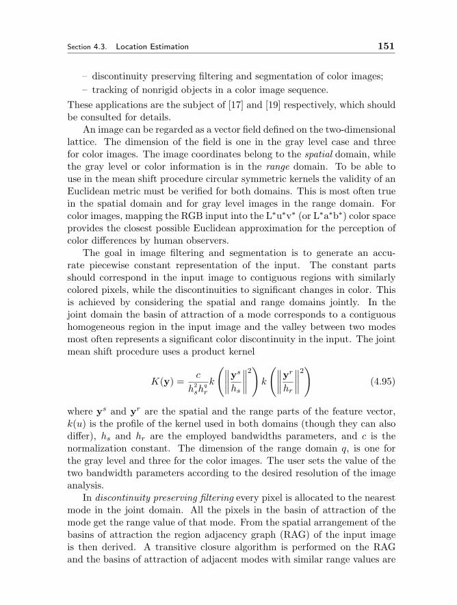
Section 4.3. Location Estimation 151
– discontinuity preserving filtering and segmentation of color images;– tracking of nonrigid objects in a color image sequence.
These applications are the subject of [17] and [19] respectively, which shouldbe consulted for details.
An image can be regarded as a vector field defined on the two-dimensionallattice. The dimension of the field is one in the gray level case and threefor color images. The image coordinates belong to the spatial domain, whilethe gray level or color information is in the range domain. To be able touse in the mean shift procedure circular symmetric kernels the validity of anEuclidean metric must be verified for both domains. This is most often truein the spatial domain and for gray level images in the range domain. Forcolor images, mapping the RGB input into the L∗u∗v∗ (or L∗a∗b∗) color spaceprovides the closest possible Euclidean approximation for the perception ofcolor differences by human observers.
The goal in image filtering and segmentation is to generate an accu-rate piecewise constant representation of the input. The constant partsshould correspond in the input image to contiguous regions with similarlycolored pixels, while the discontinuities to significant changes in color. Thisis achieved by considering the spatial and range domains jointly. In thejoint domain the basin of attraction of a mode corresponds to a contiguoushomogeneous region in the input image and the valley between two modesmost often represents a significant color discontinuity in the input. The jointmean shift procedure uses a product kernel
K(y) =c
h2sh
q
r
k
(∥∥∥∥ys
hs
∥∥∥∥2)k
(∥∥∥∥yr
hr
∥∥∥∥2)
(4.95)
where ys and yr are the spatial and the range parts of the feature vector,k(u) is the profile of the kernel used in both domains (though they can alsodiffer), hs and hr are the employed bandwidths parameters, and c is thenormalization constant. The dimension of the range domain q, is one forthe gray level and three for the color images. The user sets the value of thetwo bandwidth parameters according to the desired resolution of the imageanalysis.
In discontinuity preserving filtering every pixel is allocated to the nearestmode in the joint domain. All the pixels in the basin of attraction of themode get the range value of that mode. From the spatial arrangement of thebasins of attraction the region adjacency graph (RAG) of the input imageis then derived. A transitive closure algorithm is performed on the RAGand the basins of attraction of adjacent modes with similar range values are
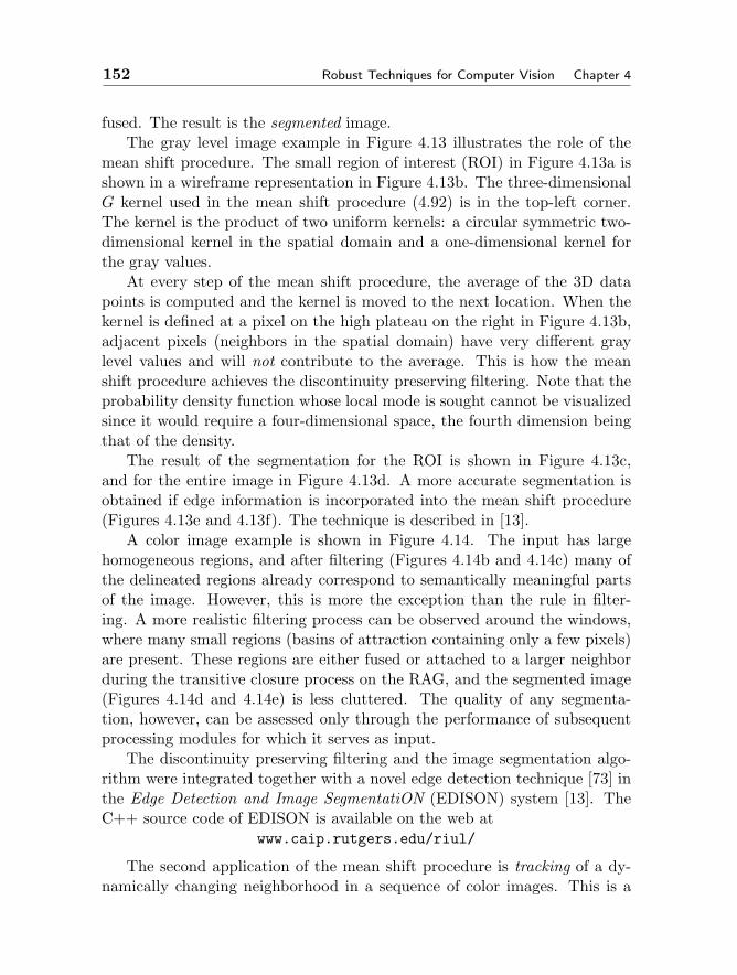
152 Robust Techniques for Computer Vision Chapter 4
fused. The result is the segmented image.The gray level image example in Figure 4.13 illustrates the role of the
mean shift procedure. The small region of interest (ROI) in Figure 4.13a isshown in a wireframe representation in Figure 4.13b. The three-dimensionalG kernel used in the mean shift procedure (4.92) is in the top-left corner.The kernel is the product of two uniform kernels: a circular symmetric two-dimensional kernel in the spatial domain and a one-dimensional kernel forthe gray values.
At every step of the mean shift procedure, the average of the 3D datapoints is computed and the kernel is moved to the next location. When thekernel is defined at a pixel on the high plateau on the right in Figure 4.13b,adjacent pixels (neighbors in the spatial domain) have very different graylevel values and will not contribute to the average. This is how the meanshift procedure achieves the discontinuity preserving filtering. Note that theprobability density function whose local mode is sought cannot be visualizedsince it would require a four-dimensional space, the fourth dimension beingthat of the density.
The result of the segmentation for the ROI is shown in Figure 4.13c,and for the entire image in Figure 4.13d. A more accurate segmentation isobtained if edge information is incorporated into the mean shift procedure(Figures 4.13e and 4.13f). The technique is described in [13].
A color image example is shown in Figure 4.14. The input has largehomogeneous regions, and after filtering (Figures 4.14b and 4.14c) many ofthe delineated regions already correspond to semantically meaningful partsof the image. However, this is more the exception than the rule in filter-ing. A more realistic filtering process can be observed around the windows,where many small regions (basins of attraction containing only a few pixels)are present. These regions are either fused or attached to a larger neighborduring the transitive closure process on the RAG, and the segmented image(Figures 4.14d and 4.14e) is less cluttered. The quality of any segmenta-tion, however, can be assessed only through the performance of subsequentprocessing modules for which it serves as input.
The discontinuity preserving filtering and the image segmentation algo-rithm were integrated together with a novel edge detection technique [73] inthe Edge Detection and Image SegmentatiON (EDISON) system [13]. TheC++ source code of EDISON is available on the web at
www.caip.rutgers.edu/riul/
The second application of the mean shift procedure is tracking of a dy-namically changing neighborhood in a sequence of color images. This is a
Section 4.3. Location Estimation 153
(a) (b)
(c) (d)
(e) (f)
Figure 4.13. The image segmentation algorithm. (a) The gray level input imagewith a region of interest (ROI) marked. (b) The wireframe representation of theROI and the 3D window used in the mean shift procedure. (c) The segmentedROI. (d) The segmented image. (e) The segmented ROI when local discontinuityinformation is integrated into the mean shift procedure. (f) The segmented image.
154 Robust Techniques for Computer Vision Chapter 4
(a)
(b) (c)
(d) (e)
Figure 4.14. A color image filtering/segmentation example. (a) The input image.(b) The filtered image. (c) The boundaries of the delineated regions. (d) Thesegmented image. (e) The boundaries of the delineated regions.
Section 4.3. Location Estimation 155
critical module in many object recognition and surveillance tasks. The prob-lem is solved by analyzing the image sequence as pairs of two consecutiveframes. See [19] for a complete discussion.
The neighborhood to be tracked, i.e., the target model in the first im-age contains na pixels. We are interested only in the amount of relativetranslation of the target between the two frames. Therefore, without loss ofgenerality the target model can be considered centered on ya = 0. In thenext frame, the target candidate is centered on yb and contains nb pixels.
In both color images kernel density estimates are computed in the jointfive-dimensional domain. In the spatial domain the estimates are definedin the center of the neighborhoods, while in the color domain the density issampled at m locations c. Let c = 1, . . . ,m be a scalar hashing index of thesethree-dimensional sample points. A kernel with profile k(u) and bandwidthsha and hb is used in the spatial domain. The sampling in the color domainis performed with the Kronecker delta function δ(u) as kernel.
The result of the two kernel density estimations are the two discrete colordensities associated with the target in the two images. For c = 1, . . . ,m
model: fa(c) = A∑na
i=1 k
(∥∥∥ya,i
ha
∥∥∥2)δ[c(ya,i)− c
](4.96)
candidate: fb(c,yb) = B∑nb
i=1 k
(∥∥∥yb−yb,i
hb
∥∥∥2)δ[c(yb,i)− c
](4.97)
where, c(y) is the color vector of the pixel at y. The normalization constantsA,B are determined such that
m∑c=1
fa(c) = 1m∑c=1
fb(c,yb) = 1 . (4.98)
The normalization assures that the template matching score between thesetwo discrete signals is
ρ(yb) =m∑c=1
√fa(c)fb(c,yb) (4.99)
and it can be shown that
d(yb) =√
1− ρ(yb) (4.100)
is a metric distance between fa(c) and fb(c,yb)To find the location of the target in the second image, the distance (4.100)
has to be minimized over yb, or equivalently (4.99) has to be maximized.
156 Robust Techniques for Computer Vision Chapter 4
That is, the local maximum of ρ(yb) has to be found by performing a searchin the second image. This search is implemented using the mean shift pro-cedure.
The local maximum is a root of the template matching score gradient
∇ρ(yb) =12
m∑c=1
∇fb(c,yb)√
fa(c)
fb(c,yb)= 0 . (4.101)
Taking into account (4.97) yields
m∑c=1
nb∑i=1
(yb−yb,i) k′(∥∥∥∥yb − yb,i
h
∥∥∥∥2)δ[c(yb,i)− c
]√ fa(c)
fb(c,yb)= 0 . (4.102)
As in Section 4.3.3 we can introduce the profile g(u) = −k′(u) and definethe weights
qi(yb) =m∑c=1
√fa(c)
fb(c,yb)δ[c(yb,i)− c
](4.103)
and obtain the iterative solution of (4.101) from
y[l+1]b =
∑nbi=1 y[l]
b,i qi
(y[l]b
)g
(∥∥∥∥y[l]b −yb,i
hb
∥∥∥∥2)
∑nbi=1 qi
(y[l]b
)g
(∥∥∥∥y[l]b −yb,i
hb
∥∥∥∥2) (4.104)
which is a mean shift procedure, the only difference being that at each stepthe weights (4.103) are also computed.
In Figure 4.15 four frames of an image sequence are shown. The tar-get model, defined in the first frame (Figure 4.15a), is successfully trackedthroughout the sequence. As can be seen, the localization is satisfactory inspite of the target candidates’ color distribution being significantly differ-ent from that of the model. While the model can be updated as we movealong the sequence, the main reason for the good performance is the smallamount of translation of the target region between two consecutive frames.The search in the second image always starts from the location of the targetmodel center in the first image. The mean shift procedure then finds thenearest mode of the template matching score, and with high probability thisis the target candidate location we are looking for. See [19] for more exam-ples and extensions of the tracking algorithm, and [14] for a version withautomatic bandwidth selection.
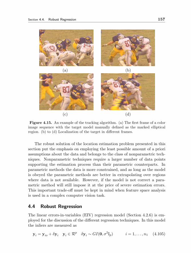
Section 4.4. Robust Regression 157
(a) (b)
(c) (d)
Figure 4.15. An example of the tracking algorithm. (a) The first frame of a colorimage sequence with the target model manually defined as the marked ellipticalregion. (b) to (d) Localization of the target in different frames.
The robust solution of the location estimation problem presented in thissection put the emphasis on employing the least possible amount of a prioriassumptions about the data and belongs to the class of nonparametric tech-niques. Nonparametric techniques require a larger number of data pointssupporting the estimation process than their parametric counterparts. Inparametric methods the data is more constrained, and as long as the modelis obeyed the parametric methods are better in extrapolating over regionswhere data is not available. However, if the model is not correct a para-metric method will still impose it at the price of severe estimation errors.This important trade-off must be kept in mind when feature space analysisis used in a complex computer vision task.
4.4 Robust Regression
The linear errors-in-variables (EIV) regression model (Section 4.2.6) is em-ployed for the discussion of the different regression techniques. In this modelthe inliers are measured as
yi = yio + δyi yi ∈ Rp δyi ∼ GI(0, σ2Ip) i = 1, . . . , n1 (4.105)
158 Robust Techniques for Computer Vision Chapter 4
and their true values obey the constraints
g(yio) = yioθ − α = 0 i = 1, . . . , n1 ‖θ‖ = 1 α ≥ 0 . (4.106)
The number of inliers must be much larger than the number of free param-eters of the model, n1 p. Nothing is assumed about the n− n1 outliers.
After a robust method selects the inliers they are often postprocessedwith a nonrobust technique from the least squares (LS) family to obtain thefinal parameter. Therefore, we start by discussing the LS estimators. Next,the family of M-estimators is introduced and the importance of the scaleparameter related to the noise of the inliers is emphasized.
All the robust regression methods popular today in computer vision canbe described within the framework of M-estimation and thus their perfor-mance also depends on the accuracy of the scale parameter. To avoid thisdeficiency, we approach M-estimation in a different way and introduce thepbM-estimator which does not require the user to provide the value of thescale.
In Section 4.2.5 it was shown that when a nonlinear EIV regression modelis processed as a linear model in the carriers, the associated noise is het-eroscedastic. Since the robust methods discussed in this section assume themodel (4.105) and (4.106), they return biased estimates if employed for solv-ing nonlinear EIV regression problems. However, this does not mean theyshould not be used! The role of any robust estimator is only to establisha satisfactory inlier/outlier dichotomy. As long as most of the inliers wererecovered from the data, postprocessing with the proper nonlinear (and non-robust) method will provide the correct estimates.
Regression in the presence of multiple structures in the data will not beconsidered beyond the particular case of two structures in the context ofstructured outliers. We will show why all the robust regression methods failto handle such data once the measurement noise becomes large.
Each of the regression techniques in this section is related to one of theobjective functions described in Section 4.2.2. Using the same objectivefunction location models can also be estimated, but we will not discuss theselocation estimators. For example, many of the traditional clustering methodsbelong to the least squares family [52, Sec.3.3.2], or there is a close connectionbetween the mean shift procedure and M-estimators of location [17].
4.4.1 Least Squares Family
We have seen in Section 4.2.3 that the least squares family of estimators isnot robust since its objective function JLS (4.22) is a symmetric function in
Section 4.4. Robust Regression 159
all the measurements. Therefore, in this section will assume that the datacontains only inliers, i.e., n = n1.
The parameter estimates of the linear EIV regression model are obtainedby solving the minimization
[ α, θ ] = argminα,θ
1n
n∑i=1
‖yi − yio‖2 = argminα,θ
1n
n∑i=1
g(yi)2 (4.107)
subject to (4.106). The minimization yields the total least squares (TLS)estimator. For an in-depth analysis of the TLS estimation see the book[111]. Related problems were already discussed in the nineteenth century[33, p.30], though the method most frequently used today, based on thesingular value decomposition (SVD) was proposed only in 1970 by Goluband Reinsch [37]. See the book [38] for the linear algebra background.
To solve the minimization problem (4.107) will define the n× p matricesof the measurements Y and of the true values Yo
Y = [y1 y2 · · · yn] Yo = [y1o y2o · · · yno]
. (4.108)
Then (4.107) can be rewritten as
[ α, θ ] = argminα,θ‖Y −Yo‖2F (4.109)
subject toYoθ − α1n = 0n (4.110)
where 1n(0n) is a vector in Rn of all ones (zeros), and ‖A‖F is the Frobeniusnorm of the matrix A.
The parameter α is eliminated next. The data is centered by using theorthogonal projector matrix G = In− 1
n1n1n which has the property G1n =
0n. It is easy to verify that
Y = GY = [y1 y2 · · · yn] yi = yi −1n
n∑i=1
yi = yi − y . (4.111)
The matrix Yo = GYo is similarly defined. The parameter estimate θ is thenobtained from the minimization
θ = argminθ‖Y − Yo‖2F (4.112)
subject toYoθ = 0n . (4.113)

160 Robust Techniques for Computer Vision Chapter 4
The constraint (4.113) implies that the rank of the true data matrix Yo isonly p− 1 and that the true θ spans its null space. Indeed, our linear modelrequires that the true data points belong to a hyperplane in Rp which is a(p− 1)-dimensional affine subspace. The vector θ is the unit normal to thisplane.
The available measurements, however, are located nearby the hyperplaneand thus the measurement matrix Y has full rank p. The solution of the TLSthus is the rank p− 1 approximation of Y . This approximation is obtainedfrom the SVD of Y written as a dyadic sum
Y =p∑
k=1
σkukvk (4.114)
where the singular vectors ui, i = 1, . . . , n and vj , j = 1, . . . , p provideorthonormal bases for the four linear subspaces associated with the matrixY [38, Sec.2.6.2], and σ1 ≥ σ2 ≥ · · · ≥ σp > 0 are the singular values of thisfull rank matrix.
The optimum approximation yielding the minimum Frobenius norm forthe error is the truncation of the dyadic sum (4.114) at p − 1 terms [111,p.31]
Y =p−1∑k=1
σkukvk (4.115)
where the matrix Y contains the centered corrected measurements y. Thesecorrected measurements are the orthogonal projections of the available yi onthe hyperplane characterized by the parameter estimates (Figure 4.6). TheTLS estimator is also known as orthogonal least squares.
The rank one null space of Y is spanned by vp, the right singular vectorassociated with the smallest singular value σp of Y [38, p.72]. Since vp is aunit vector
θ = vp . (4.116)
The estimate of α is obtained by reversing the centering operation
α = yθ . (4.117)
The parameter estimates of the linear EIV model can be also obtained ina different, though completely equivalent way. We define the carrier vectorx by augmenting the variables with a constant
x = [y − 1] σ2C = σ2[
Ip 00 0
](4.118)
Section 4.4. Robust Regression 161
which implies that the covariance matrix of the carriers is singular. Usingthe n× (p+ 1) matrices
X = [x1 x2 · · · xn] Xo = [x1o x2o · · · xno] (4.119)
the constraint (4.110) can be written as
Xoω = 0n ω = [θ α] ‖θ‖ = 1 α ≥ 0 (4.120)
where the subscript ‘1’ of this parametrization in Section 4.2.6 was dropped.Using Lagrangian multipliers it can be shown that the parameter estimate
ω is the eigenvector of the generalized eigenproblem
XXω = λCω (4.121)
corresponding to the smallest eigenvalue λmin. This eigenproblem is equiva-lent to the definition of the right singular values of the matrix Y [38, Sec.8.3].The condition ‖θ‖ = 1 is then imposed on the vector ω.
The first order approximation for the covariance of the parameter esti-mate is [70, Sec.5.2.2]
Cω = σ2(XX− λminC)+ (4.122)
where the pseudoinverse has to be used since the matrix has rank p following(4.121). The estimate of the noise standard deviation is
σ2 =∑n
i=1 g(yi)2
n− p+ 1=
λminn− p+ 1
=σ2p
n− p+ 1(4.123)
where g(yi) = yi θ − α are the residuals. The covariances for the other
parametrizations of the linear EIV model, ω2 (4.53) and ω3 (4.55) can beobtained through error propagation.
Note that when computing the TLS estimate with either of the two meth-ods, special care has to be taken to execute all the required processing steps.The first approach starts with the data being centered, while in the sec-ond approach a generalized eigenproblem has to be solved. These steps aresometimes neglected in computer vision algorithms.
In the traditional linear regression model only the variable z is corruptedby noise (4.36), and the constraint is
zio = α+ xioθ xio = x(yio) i = 1, . . . , n . (4.124)
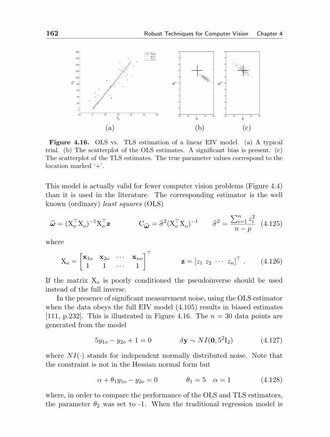
162 Robust Techniques for Computer Vision Chapter 4
−10 0 10 20 30 40 50
0
20
40
60
80
100
120
140
160
180
y1
y 2
TrueOLSTLS
−40 −20 0 20 40−2
−1
0
1
2
3
4
5
6
7
8
α
θ 1
−40 −20 0 20 40−2
−1
0
1
2
3
4
5
6
7
8
α
θ 1
(a) (b) (c)
Figure 4.16. OLS vs. TLS estimation of a linear EIV model. (a) A typicaltrial. (b) The scatterplot of the OLS estimates. A significant bias is present. (c)The scatterplot of the TLS estimates. The true parameter values correspond to thelocation marked ‘+’.
This model is actually valid for fewer computer vision problems (Figure 4.4)than it is used in the literature. The corresponding estimator is the wellknown (ordinary) least squares (OLS)
ω = (Xo Xo)
−1Xo z Cω = σ2(X
o Xo)−1 σ2 =
∑ni=1 z
2i
n− p (4.125)
where
Xo =[x1o x2o · · · xno1 1 · · · 1
]z = [z1 z2 · · · zn] . (4.126)
If the matrix Xo is poorly conditioned the pseudoinverse should be usedinstead of the full inverse.
In the presence of significant measurement noise, using the OLS estimatorwhen the data obeys the full EIV model (4.105) results in biased estimates[111, p.232]. This is illustrated in Figure 4.16. The n = 30 data points aregenerated from the model
5y1o − y2o + 1 = 0 δy ∼ NI(0, 52I2) (4.127)
where NI(·) stands for independent normally distributed noise. Note thatthe constraint is not in the Hessian normal form but
α+ θ1y1o − y2o = 0 θ1 = 5 α = 1 (4.128)
where, in order to compare the performance of the OLS and TLS estimators,the parameter θ2 was set to -1. When the traditional regression model is
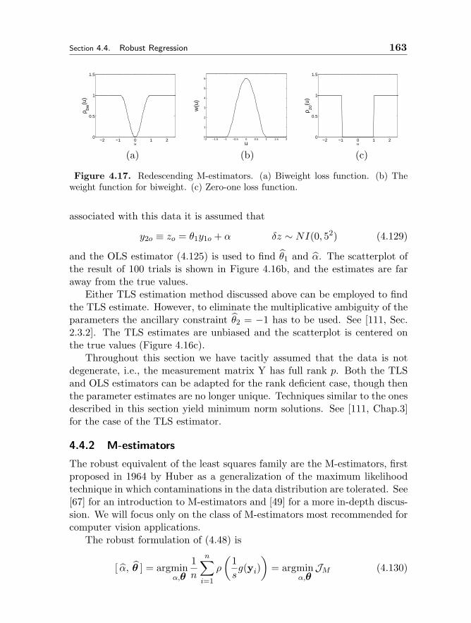
Section 4.4. Robust Regression 163
−2 −1 0 1 20
0.5
1
1.5
u
ρ bw(u
)
−2 −1.5 −1 −0.5 0 0.5 1 1.5 20
1
2
3
4
5
6
u
w(u
)
−2 −1 0 1 20
0.5
1
1.5
u
ρ zo(u
)
(a) (b) (c)
Figure 4.17. Redescending M-estimators. (a) Biweight loss function. (b) Theweight function for biweight. (c) Zero-one loss function.
associated with this data it is assumed that
y2o ≡ zo = θ1y1o + α δz ∼ NI(0, 52) (4.129)
and the OLS estimator (4.125) is used to find θ1 and α. The scatterplot ofthe result of 100 trials is shown in Figure 4.16b, and the estimates are faraway from the true values.
Either TLS estimation method discussed above can be employed to findthe TLS estimate. However, to eliminate the multiplicative ambiguity of theparameters the ancillary constraint θ2 = −1 has to be used. See [111, Sec.2.3.2]. The TLS estimates are unbiased and the scatterplot is centered onthe true values (Figure 4.16c).
Throughout this section we have tacitly assumed that the data is notdegenerate, i.e., the measurement matrix Y has full rank p. Both the TLSand OLS estimators can be adapted for the rank deficient case, though thenthe parameter estimates are no longer unique. Techniques similar to the onesdescribed in this section yield minimum norm solutions. See [111, Chap.3]for the case of the TLS estimator.
4.4.2 M-estimators
The robust equivalent of the least squares family are the M-estimators, firstproposed in 1964 by Huber as a generalization of the maximum likelihoodtechnique in which contaminations in the data distribution are tolerated. See[67] for an introduction to M-estimators and [49] for a more in-depth discus-sion. We will focus only on the class of M-estimators most recommended forcomputer vision applications.
The robust formulation of (4.48) is
[ α, θ ] = argminα,θ
1n
n∑i=1
ρ
(1sg(yi)
)= argmin
α,θJM (4.130)

164 Robust Techniques for Computer Vision Chapter 4
where s is a parameter which depends on σ, the (unknown) scale of theinlier noise (4.105). With a slight abuse of notation s will also be calledscale. The loss function ρ(u) satisfies the following properties: nonnegativewith ρ(0) = 0, even symmetric ρ(u) = ρ(−u), and nondecreasing with |u|.For ρ(u) = u2 we obtain the LS objective function (4.107).
The different M-estimators introduced in the statistical literature differthrough the distribution assumed for the data. See [5] for a discussion in thecontext of computer vision. However, none of these distributions will providean accurate model in a real application. Thus, the distinctive theoreticalproperties of different M-estimators are less relevant in practice.
The redescending M-estimators are characterized by bounded loss func-tions
0 ≤ ρ(u) ≤ 1 |u| ≤ 1 ρ(u) = 1 |u| > 1 . (4.131)
As will be shown below, in a redescending M-estimator only those data pointswhich are at distance less than s from the current fit are taken into account.This yields better outlier rejection properties than that of the M-estimatorswith nonredescending loss functions [69], [115].
The following class of redescending loss functions covers several impor-tant M-estimators
ρ(u) =
1− (1− u2)d |u| ≤ 11 |u| > 1
(4.132)
where d = 1, 2, 3. The loss functions have continuous derivatives up the(d− 1)-th order, and a unique minimum in ρ(0) = 0.
Tukey’s biweight function ρbw(u) (Figure 4.17a) is obtained for d = 3 [67,p.295]. This loss function is widely used in the statistical literature and wasknown at least a century before robust estimation [40, p.151]. See also [42,vol.I, p.323]. The loss function obtained for d = 2 will be denoted ρe(u).The case d = 1 yields the skipped mean loss function, a name borrowed fromrobust location estimators [89, p.181]
ρsm(u) =u2 |u| ≤ 11 |u| > 1
(4.133)
which has discontinuous first derivative. It is often used in vision applica-tions, e.g., [108].
In the objective function of any M-estimator the geometric distances(4.46) are normalized by the scale s. Since ρ(u) is an even function we donot need to use absolute values in (4.130). In redescending M-estimators thescale acts as a hard rejection threshold, and thus its value is of paramount
Section 4.4. Robust Regression 165
importance. For the moment we will assume that a satisfactory value isalready available for s, but will return to this topic in Section 4.4.3.
The M-estimator equivalent to the total least squares is obtained follow-ing either TLS method discussed in Section 4.4.1. For example, it can beshown that instead of (4.121), the M-estimate of ω (4.120) is the eigenvectorcorresponding to the the smallest eigenvalue of the generalized eigenproblem
XWXω = λCω (4.134)
where W ∈ Rn×n is the diagonal matrix of the nonnegative weights
wi = w(ui) =1ui
dρ(ui)du
≥ 0 ui =g(yi)s
i = 1, . . . , n . (4.135)
Thus, in redescending M-estimators w(u) = 0 for |u| > 1, i.e., the data pointswhose residual g(yi) = y
i θ − α relative to the current fit is larger than thescale threshold s are discarded from the computations. The weights wbw(u) =6(1−u2)2 derived from the biweight loss function are shown in Figure 4.17b.The weigths derived from the ρe(u) loss function are proportional to theEpanechnikov kernel (4.79). For traditional regression instead of (4.125) theM-estimate is
ω = (Xo WXo)
−1Xo Wz . (4.136)
The residuals g(yi) in the weights wi require values for the parameter esti-mates. Therefore, the M-estimates can be found only by an iterative proce-dure.
M-estimation with Iterative Weighted Least SquaresGiven the scale s.
1. Obtain the initial parameter estimate ω[0] with total least squares.
2. Compute the weights w[l+1]i , l = 0, 1, . . ..
3. Obtain the updated parameter estimates, ω[l+1].
4. Verify if ‖ω[l+1] − ω[l]‖ is less than the tolerance. If yes, stop.
5. Replace ω[l] with ω[l+1]. Return to Step 2.
For the traditional regression the procedure is identical. See [67, p.306]. Adifferent way of computing linear EIV regression M-estimates is described in[115].
The objective function minimized for redescending M-estimators is notconvex, and therefore the convergence to a global minimum is not guaran-teed. Nevertheless, in practice convergence is always achieved [67, p.307],
166 Robust Techniques for Computer Vision Chapter 4
and if the initial fit and the chosen scale value are adequate, the obtainedsolution is satisfactory. These two conditions are much more influential thanthe precise nature of the employed loss function. Note that at every itera-tion all the data points regarded as inliers are processed, and thus there isno need for postprocessing, as is the case with the elemental subsets basednumerical optimization technique discussed in Section 4.2.7.
In the statistical literature often the scale threshold s is defined as theproduct between σ the robust estimate for the standard deviation of theinlier noise (4.105) and a tuning constant. The tuning constant is derivedfrom the asymptotic properties of the simplest location estimator, the mean[67, p.296]. Therefore its value is rarely meaningful in real applications.Our definition of redescending M-estimators avoids the problem of tuningby using the inlier/outlier classification threshold as the scale parameter s.
The case d = 0 in (4.132) yields the zero-one loss function
ρzo(u) =
0 |u| ≤ 11 |u| > 1
(4.137)
shown in Figure 4.17c. The zero-one loss function is also a redescendingM-estimator, however, is no longer continuous and does not have a uniqueminimum in u = 0. It is only mentioned since in Section 4.4.4 will beused to link the M-estimators to other robust regression techniques suchas LMedS or RANSAC. The zero-one M-estimator is not recommended inapplications. The weight function (4.135) is nonzero only at the boundaryand the corresponding M-estimator has poor local robustness properties.That is, in a critical data configuration a single data point can have a verylarge influence on the parameter estimates.
4.4.3 Median Absolute Deviation Scale Estimate
Access to a reliable scale parameter s is a necessary condition for the mini-mization procedure (4.130) to succeed. The scale s is a strictly monotonicallyincreasing function of σ the standard deviation of the inlier noise. Since σ isa nuisance parameter of the model, it can be estimated together with α andθ at every iteration of the M-estimation process [67, p.307]. An example ofa vision application employing this approach is [7]. However, the strategyis less robust than providing the main estimation process with a fixed scalevalue [68]. In the latter case we talk about an M-estimator with auxiliaryscale [69], [100].
Two different approaches can be used to obtain the scale prior to theparameter estimation. It can be either arbitrarily set by the user, or it can be
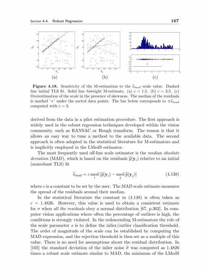
Section 4.4. Robust Regression 167
0 50 100 150 200 250
−100
−50
0
50
100
150
y1
y 2
0 50 100 150 200 250
−100
−50
0
50
100
150
y1
y 2
−4 −2 0 2 4 6 8 100
5
10
15
20
25
−4 −2 0 2 4 6 8 10−0.5
−0.4
−0.3
−0.2
−0.1
0
0.1
(a) (b) (c)
Figure 4.18. Sensitivity of the M-estimation to the smad scale value. Dashedline–initial TLS fit. Solid line–biweight M-estimate. (a) c = 1.5. (b) c = 3.5. (c)Overestimation of the scale in the presence of skewness. The median of the residualsis marked ‘+’ under the sorted data points. The bar below corresponds to ±smad
computed with c = 3.
derived from the data in a pilot estimation procedure. The first approach iswidely used in the robust regression techniques developed within the visioncommunity, such as RANSAC or Hough transform. The reason is that itallows an easy way to tune a method to the available data. The secondapproach is often adopted in the statistical literature for M-estimators andis implicitly employed in the LMedS estimator.
The most frequently used off-line scale estimator is the median absolutedeviation (MAD), which is based on the residuals g(yi) relative to an initial(nonrobust TLS) fit
smad = cmedi|g(yi)−med
jg(yj)| (4.138)
where c is a constant to be set by the user. The MAD scale estimate measuresthe spread of the residuals around their median.
In the statistical literature the constant in (4.138) is often taken asc = 1.4826. However, this value is used to obtain a consistent estimatefor σ when all the residuals obey a normal distribution [67, p.302]. In com-puter vision applications where often the percentage of outliers is high, theconditions is strongly violated. In the redescending M-estimators the role ofthe scale parameter s is to define the inlier/outlier classification threshold.The order of magnitude of the scale can be established by computing theMAD expression, and the rejection threshold is then set as a multiple of thisvalue. There is no need for assumptions about the residual distribution. In[105] the standard deviation of the inlier noise σ was computed as 1.4826times a robust scale estimate similar to MAD, the minimum of the LMedS
168 Robust Techniques for Computer Vision Chapter 4
optimization criterion (4.140). The rejection threshold was set at 1.96σ byassuming normally distributed residuals. The result is actually three timesthe computed MAD value, and could be obtained by setting c = 3 withoutany assumption about the distribution of the residuals.
The example in Figures 4.18a and 4.18b illustrates not only the impor-tance of the scale value for M-estimation but also the danger of being lockedinto the nature of the residuals. The data contains 100 inliers and 75 out-liers, and as expected the initial TLS fit is completely wrong. When thescale parameter is set small by choosing for smad the constant c = 1.5, atconvergence the final M-estimate is satisfactory (Figure 4.18a). When thescale smad is larger, c = 3.5, the optimization process converges to a localminimum of the objective function. This minimum does not correspond to arobust fit (Figure 4.18b). Note that c = 3.5 is about the value of the constantwhich would have been used under the assumption of normally distributedinlier noise.
The location estimator employed for centering the residuals in (4.138) isthe median, while the MAD estimate is computed with the second, outermedian. However, the median is a reliable estimator only when the distri-bution underlying the data is unimodal and symmetric [49, p.29]. It is easyto see that for a heavily skewed distribution, i.e., with a long tail on oneside, the median will be biased toward the tail. For such distributions theMAD estimator severely overestimates the scale since the 50th percentileof the centered residuals is now shifted toward the boundary of the inlierdistribution. The tail is most often due to outliers, and the amount of over-estimation increases with both the decrease of the inlier/outlier ratio andthe lengthening of the tail. In the example in Figure 4.18c the inliers (atthe left) were obtained from a standard normal distribution. The median is0.73 instead of zero. The scale computed with c = 3 is smad = 4.08 which inmuch larger than 2.5, a reasonable value for the spread of the inliers. Again,c should be chosen smaller.
Scale estimators which avoid centering the data were proposed in thestatistical literature [88], but they are computationally intensive and theiradvantage for vision applications is not immediate. We must conclude thatthe MAD scale estimate has to be used with care in robust algorithms dealingwith real data. Whenever available, independent information provided bythe problem at hand should be exploited to validate the obtained scale. Theinfluence of the scale parameter s on the performance of M-estimators canbe entirely avoided by a different approach toward this family of robustestimators. This will be discussed in Section 4.4.5.
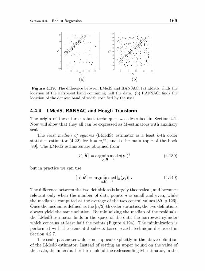
Section 4.4. Robust Regression 169
0 50 100 150 200 250
−100
−50
0
50
100
150
y1
y 2
0 50 100 150 200
−40
−20
0
20
40
60
80
100
120
140
160
y1
y 2
(a) (b)
Figure 4.19. The difference between LMedS and RANSAC. (a) LMeds: finds thelocation of the narrowest band containing half the data. (b) RANSAC: finds thelocation of the densest band of width specified by the user.
4.4.4 LMedS, RANSAC and Hough Transform
The origin of these three robust techniques was described in Section 4.1.Now will show that they all can be expressed as M-estimators with auxiliaryscale.
The least median of squares (LMedS) estimator is a least k-th orderstatistics estimator (4.22) for k = n/2, and is the main topic of the book[89]. The LMedS estimates are obtained from
[ α, θ ] = argminα,θ
medig(yi)
2 (4.139)
but in practice we can use
[ α, θ ] = argminα,θ
medi|g(yi)| . (4.140)
The difference between the two definitions is largely theoretical, and becomesrelevant only when the number of data points n is small and even, whilethe median is computed as the average of the two central values [89, p.126].Once the median is defined as the [n/2]-th order statistics, the two definitionsalways yield the same solution. By minimizing the median of the residuals,the LMedS estimator finds in the space of the data the narrowest cylinderwhich contains at least half the points (Figure 4.19a). The minimization isperformed with the elemental subsets based search technique discussed inSection 4.2.7.
The scale parameter s does not appear explicitly in the above definitionof the LMedS estimator. Instead of setting an upper bound on the value ofthe scale, the inlier/outlier threshold of the redescending M-estimator, in the
170 Robust Techniques for Computer Vision Chapter 4
LMedS a lower bound on the percentage of inliers (fifty percent) is imposed.This eliminates the need for the user to guess the amount of measurementnoise, and as long as the inliers are in absolute majority, a somewhat bet-ter robust behavior is obtained. For example, the LMedS estimator willsuccessfully process the data in Figure 4.18a.
The relation between the scale parameter and the bound on the percent-age of inliers is revealed if the equivalent condition of half the data pointsbeing outside of the cylinder, is written as
1n
n∑i=1
ρzo
(1sg(yi)
)=
12
(4.141)
where ρzo is the zero-one loss function (4.137), and the scale parameter isnow regarded as a function of the residuals s [g(y1), . . . , g(yn)]. By definings = med
i|g(yi)| the LMedS estimator becomes
[ α, θ ] = argminα,θ
s [g(y1), . . . , g(yn)] subject to (4.141). (4.142)
The new definition of LMedS is a particular case of the S-estimators, whichwhile popular in statistics, are not widely know in the vision community. Foran introduction to S-estimators see [89, pp.135–143], and for a more detailedtreatment in the context of EIV models [115]. Let s be the minimum of s in(4.142). Then, it can be shown that
[ α, θ ] = argminα,θ
1n
n∑i=1
ρzo
(1sg(yi)
)(4.143)
and thus the S-estimators are in fact M-estimators with auxiliary scale.The value of s can also be used as a scale estimator for the noise corrupt-
ing the inliers. All the observations made in Section 4.4.3 remain valid. Forexample, when the inliers are no longer the absolute majority in the data theLMedS fit is incorrect, and the residuals used to compute s are not reliable.
The Random Sample Consensus (RANSAC) estimator predates the LMedS[26]. Since the same elemental subsets based procedure is used to optimizetheir objective function, sometimes the two techniques were mistakenly con-sidered as being very similar, e.g., [74]. However, their similarity should bejudged examining the objective functions and not the way the optimizationis implemented. In LMedS the scale is computed from a condition set onthe percentage of inliers (4.142). In RANSAC the following minimization
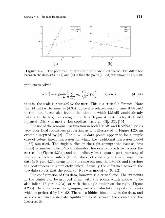
Section 4.4. Robust Regression 171
0 5 10 150
5
10
15
20
y
z
OLSLMedSFinal
0 5 10 150
5
10
15
20
y
z
OLSLMedSFinal
(a) (b)
Figure 4.20. The poor local robustness of the LMedS estimator. The differencebetween the data sets in (a) and (b) is that the point (6, 9.3) was moved to (6, 9.2).
problem is solved
[ α, θ ] = argminα,θ
1n
n∑i=1
ρzo
(1sg(yi)
)given s (4.144)
that is, the scale is provided by the user. This is a critical difference. Notethat (4.144) is the same as (4.30). Since it is relative easy to tune RANSACto the data, it can also handle situations in which LMedS would alreadyfail due to the large percentage of outliers (Figure 4.19b). Today RANSACreplaced LMedS in most vision applications, e.g., [65], [83], [107].
The use of the zero-one loss function in both LMedS and RANSAC yieldsvery poor local robustness properties, as it is illustrated in Figure 4.20, anexample inspired by [2]. The n = 12 data points appear to be a simplecase of robust linear regression for which the traditional regression model(4.37) was used. The single outlier on the right corrupts the least squares(OLS) estimator. The LMedS estimator, however, succeeds to recover thecorrect fit (Figure 4.20a), and the ordinary least squares postprocessing ofthe points declared inliers (Final), does not yield any further change. Thedata in Figure 4.20b seems to be the same but now the LMedS, and thereforethe postprocessing, completely failed. Actually the difference between thetwo data sets is that the point (6, 9.3) was moved to (6, 9.2).
The configuration of this data, however, is a critical one. The six pointsin the center can be grouped either with the points which appear to bealso inliers (Figure 4.20a), or with the single outlier on the right (Figure4.20b). In either case the grouping yields an absolute majority of pointswhich is preferred by LMedS. There is a hidden bimodality in the data, andas a consequence a delicate equilibrium exist between the correct and theincorrect fit.

172 Robust Techniques for Computer Vision Chapter 4
In this example the LMedS minimization (4.140) seeks the narrowestband containing at least six data points. The width of the band is measuredalong the z axis, and its boundary is always defined by two of the datapoints [89, p.126]. This is equivalent to using the zero-one loss function inthe optimization criterion (4.143). A small shift of one of the points thuscan change to which fit does the value of the minimum in (4.140) correspondto. The instability of the LMedS is discussed in a practical setting in [45],while more theoretical issues are addressed in [23]. A similar behavior is alsopresent in RANSAC due to (4.144).
For both LMedS and RANSAC several variants were introduced in whichthe zero-one loss function is replaced by a smooth function. Since then morepoint have nonzero weights in the optimization, the local robustness proper-ties of the estimators improve. The least trimmed squares (LTS) estimator[89, p.132]
[ α, θ ] = argminα,θ
k∑i=1
g(y)2i:n (4.145)
minimizes the sum of squares of the k smallest residuals, where k has to beprovided by the user. Similar to LMedS, the absolute values of the residualscan also be used.
In the first smooth variant of RANSAC the zero-one loss function was re-placed with the skipped mean (4.133), and was called MSAC [108]. Recentlythe same loss function was used in a maximum a posteriori formulation ofRANSAC, the MAPSAC estimator [104]. A maximum likelihood motivatedvariant, the MLESAC [106], uses a Gaussian kernel for the inliers. Guidedsampling is incorporated into the IMPSAC version of RANSAC [104]. In ev-ery variant of RANSAC the user has to provide a reasonably accurate scalevalue for a satisfactory performance.
The use of zero-one loss function is not the only (or main) cause of thefailure of LMedS (or RANSAC). In Section 4.4.7 we show that there is a moregeneral problem in applying robust regression methods to multistructureddata.
The only robust method designed to handle multistructured data is theHough transform. The idea of Hough transform is to replace the regressionproblems in the input domain with location problems in the space of theparameters. Then, each significant mode in the parameter space correspondsto an instance of the model in the input space. There is a huge literaturededicated to every conceivable aspect of this technique. The survey papers[50], [62], [81] contain hundreds of references.
Since we are focusing here on the connection between the redescending M-
Section 4.4. Robust Regression 173
estimators and the Hough transform, only the randomized Hough transform(RHT) will be considered [56]. Their equivalence is the most straightforward,but the same equivalence also exists for all the other variants of the Houghtransform as well. The feature space in RHT is built with elemental subsets,and thus we have a mapping from p data points to a point in the parameterspace.
Traditionally the parameter space is quantized into bins, i.e., it is anaccumulator. The bins containing the largest number of votes yield theparameters of the significant structures in the input domain. This can bedescribed formally as
[ α, β ]k = argmax[α,β]
k1n
n∑i=1
κzo(sα, sβ1 , . . . , sβp−1 ; g(yi)
)(4.146)
where κzo(u) = 1−ρzo(u) and sα, sβ1 , . . . , sβp−1 define the size (scale) of a binalong each parameter coordinate. The index k stands for the different localmaxima. Note that the parametrization uses the polar angles as discussedin Section 4.2.6.
The definition (4.146) is that of a redescending M-estimator with aux-iliary scale, where the criterion is a maximization instead of a minimiza-tion. The accuracy of the scale parameters is a necessary condition for asatisfactory performance, an issue widely discussed in the Hough transformliterature. The advantage of distributing the votes around adjacent bins wasrecognized early [101]. Later the equivalence with M-estimators was alsoidentified, and the zero-one loss function is often replaced with a continuousfunction [61], [60], [79].
In this section we have shown that all the robust techniques popular incomputer vision can be reformulated as M-estimators. In Section 4.4.3 wehave emphasized that the scale has a crucial influence on the performance ofM-estimators. In the next section we remove this dependence by approachingthe M-estimators in a different way.
4.4.5 The pbM-estimator
The minimization criterion (4.130) of the M-estimators is rewritten as
[ α, θ ] = argmaxα,θ
1n
n∑i=1
κ
(yi θ − αs
)κ(u) = cρ[1− ρ(u)] (4.147)
where κ(u) is called the M-kernel function. Note that for a redescending M-estimator κ(u) = 0 for |u| > 1 (4.131). The positive normalization constantcρ assures that κ(u) is a proper kernel (4.68).
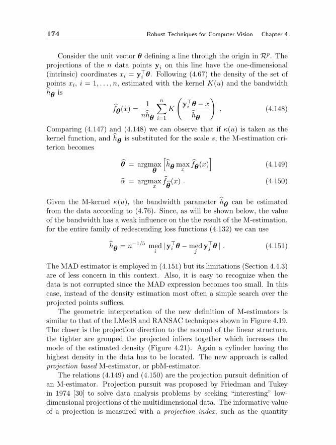
174 Robust Techniques for Computer Vision Chapter 4
Consider the unit vector θ defining a line through the origin in Rp. Theprojections of the n data points yi on this line have the one-dimensional(intrinsic) coordinates xi = y
i θ. Following (4.67) the density of the set ofpoints xi, i = 1, . . . , n, estimated with the kernel K(u) and the bandwidthhθ is
fθ(x) =1
nhθ
n∑i=1
K
(yi θ − xhθ
). (4.148)
Comparing (4.147) and (4.148) we can observe that if κ(u) is taken as thekernel function, and hθ is substituted for the scale s, the M-estimation cri-terion becomes
θ = argmaxθ
[hθ max
xfθ(x)
](4.149)
α = argmaxx
fθ(x) . (4.150)
Given the M-kernel κ(u), the bandwidth parameter hθ can be estimatedfrom the data according to (4.76). Since, as will be shown below, the valueof the bandwidth has a weak influence on the the result of the M-estimation,for the entire family of redescending loss functions (4.132) we can use
hθ = n−1/5 medi|y
i θ −medj
yj θ | . (4.151)
The MAD estimator is employed in (4.151) but its limitations (Section 4.4.3)are of less concern in this context. Also, it is easy to recognize when thedata is not corrupted since the MAD expression becomes too small. In thiscase, instead of the density estimation most often a simple search over theprojected points suffices.
The geometric interpretation of the new definition of M-estimators issimilar to that of the LMedS and RANSAC techniques shown in Figure 4.19.The closer is the projection direction to the normal of the linear structure,the tighter are grouped the projected inliers together which increases themode of the estimated density (Figure 4.21). Again a cylinder having thehighest density in the data has to be located. The new approach is calledprojection based M-estimator, or pbM-estimator.
The relations (4.149) and (4.150) are the projection pursuit definition ofan M-estimator. Projection pursuit was proposed by Friedman and Tukeyin 1974 [30] to solve data analysis problems by seeking “interesting” low-dimensional projections of the multidimensional data. The informative valueof a projection is measured with a projection index, such as the quantity
Section 4.4. Robust Regression 175
0 200 400 600 800 1000
−100
0
100
200
300
400
500
600
700
800
θ1
θ2
y1
y 2
200 300 400 500 600 700 800 900 10000
0.005
0.01
0.015
x
f θ 1(x)
200 300 400 500 600 700 800 900 10000
0.005
0.01
0.015
x
f θ 2(x)
(a) (b) (c)
Figure 4.21. M-estimation through projection pursuit. When the data in therectangle is projected orthogonally on different directions (a), the mode of the esti-mated density is smaller for an arbitrary direction (b), than for the direction of thenormal to the linear structure (c).
inside the brackets in (4.149). The papers [48] [54] survey all the relatedtopics. It should be emphasized that in the projection pursuit literature thename projection pursuit regression refers to a technique different from ours.There, a nonlinear additive model is estimated by adding a new term to themodel after each iteration, e.g., [44, Sec.11.2].
When in the statistical literature a linear regression problem is solvedthrough projection pursuit, either nonrobustly [20], or robustly [89, p.143],the projection index is a scale estimate. Similar to the S-estimators thesolution is obtained by minimizing the scale, now over the projection direc-tions. The robust scale estimates, like the MAD (4.138) or the median ofthe absolute value of the residuals (4.142), however, have severe deficienciesfor skewed distributions, as was discussed in Section 4.4.3. Thus, their useas projection index will not guarantee a better performance than that of theoriginal implementation of the regression technique.
Projections were employed before in computer vision. In [80] a highlyaccurate implementation of the Hough transform was achieved by using lo-cal projections of the pixels onto a set of directions. Straight edges in theimage were then found by detecting the maxima in the numerically differen-tiated projections. The L2E estimator, proposed recently in the statisticalliterature [91], solves a minimization problem similar to the kernel density es-timate formulation of M-estimators, however, the focus is on the parametricmodel of the inlier residual distribution.
The critical parameter of the redescending M-estimators is the scale s,the inlier/outlier selection threshold. The novelty of the pbM-estimator isthe way the scale parameter is manipulated. The pbM-estimator avoids theneed of M-estimators for an accurate scale prior to estimation by using the

176 Robust Techniques for Computer Vision Chapter 4
bandwidth hθ as scale during the search for the optimal projection direc-tion. The bandwidth being an approximation of the AMISE optimal solution(4.75) tries to preserve the sensitivity of the density estimation process asthe number of data points n becomes large. This is the reason for the n−1/5
factor in (4.151). Since hθ is the outlier rejection threshold at this stage, atoo small value increases the probability of assigning incorrectly the optimalprojection direction to a local alignment of points. Thus, it is recommendedthat once n becomes large, say n > 103, the computed bandwith value isslightly increased by a factor which is monotonic in n.
After the optimal projection direction θ was found, the actual inlier/outlierdichotomy of the data is defined by analyzing the shape of the density aroundthe mode. The nearest local minima on the left and on the right correspondin Rp, the space of the data, to the transition between the inliers belongingto the sought structure (which has a higher density) and the backgroundclutter of the outliers (which has a lower density). The locations of theminima define the values α1 < α2. Together with θ they yield the twohyperplanes in Rp separating the inliers from the outliers. Note that theequivalent scale of the M-estimator is s = α2−α1, and that the minima maynot be symmetrically located relative to the mode.
The 2D data in the example in Figure 4.22a contains 100 inliers and 500outliers. The density of the points projected on the direction of the truenormal (Figure 4.22b) has a sharp mode. Since the pbM-estimator dealsonly with one-dimensional densities, there is no need to use the mean shiftprocedure (Section 4.3.3) to find the modes, and a simple heuristic sufficesto define the local minima if they are not obvious.
The advantage of the pbM-estimator arises from using a more adequatescale in the optimization. In our example, the smad scale estimate based onthe TLS initial fit (to the whole data) and computed with c = 3, is aboutten times larger than h
θ, the bandwith computed for the optimal projection
direction (Figure 4.22b). When a redescending M-estimator uses smad, theoptimization of the objective function is based on a too large band, whichalmost certainly leads to a nonrobust behavior.
Sometimes the detection of the minima can be fragile. See the right mini-mum in Figure 4.22b. A slight change in the projected location of a few datapoints could have changed this boundary to the next, much more significantlocal minimum. However, this sensitivity is tolerated by pbM-estimator.First, by the nature of the projection pursuit many different projections areinvestigated and thus it is probable that at least one satisfactory band isfound. Second, from any reasonable inlier/outlier dichotomy of the data
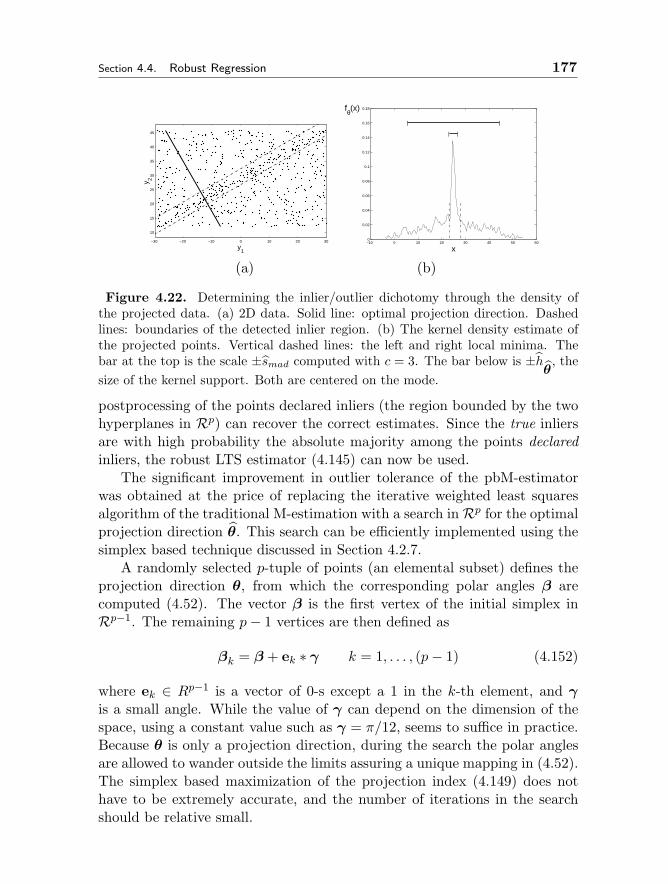
Section 4.4. Robust Regression 177
−30 −20 −10 0 10 20 30
10
15
20
25
30
35
40
45
y1
y 2
−10 0 10 20 30 40 50 600
0.02
0.04
0.06
0.08
0.1
0.12
0.14
0.16
0.18
x
fθ(x)
| |
| |
(a) (b)
Figure 4.22. Determining the inlier/outlier dichotomy through the density ofthe projected data. (a) 2D data. Solid line: optimal projection direction. Dashedlines: boundaries of the detected inlier region. (b) The kernel density estimate ofthe projected points. Vertical dashed lines: the left and right local minima. Thebar at the top is the scale ±smad computed with c = 3. The bar below is ±h
θ, the
size of the kernel support. Both are centered on the mode.
postprocessing of the points declared inliers (the region bounded by the twohyperplanes in Rp) can recover the correct estimates. Since the true inliersare with high probability the absolute majority among the points declaredinliers, the robust LTS estimator (4.145) can now be used.
The significant improvement in outlier tolerance of the pbM-estimatorwas obtained at the price of replacing the iterative weighted least squaresalgorithm of the traditional M-estimation with a search inRp for the optimalprojection direction θ. This search can be efficiently implemented using thesimplex based technique discussed in Section 4.2.7.
A randomly selected p-tuple of points (an elemental subset) defines theprojection direction θ, from which the corresponding polar angles β arecomputed (4.52). The vector β is the first vertex of the initial simplex inRp−1. The remaining p− 1 vertices are then defined as
βk = β + ek ∗ γ k = 1, . . . , (p− 1) (4.152)
where ek ∈ Rp−1 is a vector of 0-s except a 1 in the k-th element, and γis a small angle. While the value of γ can depend on the dimension of thespace, using a constant value such as γ = π/12, seems to suffice in practice.Because θ is only a projection direction, during the search the polar anglesare allowed to wander outside the limits assuring a unique mapping in (4.52).The simplex based maximization of the projection index (4.149) does nothave to be extremely accurate, and the number of iterations in the searchshould be relative small.
178 Robust Techniques for Computer Vision Chapter 4
The projection based implementation of the M-estimators is summarizedbelow.
The pbM-estimator
– Repeat N times:1. choose an elemental subset (p-tuple) by random sampling;
2. compute the TLS estimate of θ;
3. build the initial simplex in the space of polar angles β;
4. perform a simplex based direct search to find the local maximumof the projection index.
– Find the left and right local minima around the mode of the densitycorresponding to the largest projection index.
– Define the inlier/outlier dichotomy of the data. Postprocess the inliersto find the final estimates of α and θ.
4.4.6 Applications
The superior outlier tolerance of the pbM-estimator relative to other robusttechniques is illustrated with two experiments. The percentage of inliers inthe data is assumed unknown and can be significantly less than that of theoutliers. Therefore the LMedS estimator cannot be applied. It is shownin [106] that MLESAC and MSAC have very similar performance and aresuperior to RANSAC. We have compared RANSAC and MSAC with thepbM-estimator.
In both experiments ground truth was available, and the true standarddeviation of the inliers σt could be computed. The output of any robustregression is the inlier/outlier dichotomy of the data. Let the standard de-viation of the points declared inliers measured relative to the true fit be σin.The performance of the different estimators was compared through the ratioσin/σt. For a satisfactory result this ratio should be very close to one.
The same number of computational units is used for all the techniques. Acomputational unit is either processing of one elemental subset (RANSAC),or one iteration in the simplex based direct search (pbM). The number ofiterations in a search was restricted to 25, but often it ended earlier. Thus,the amount of computations attributed to the pbM-estimator is an upperbound.
In the first experiment the synthetic data contained 100 inlier pointsobeying an eight-dimensional linear EIV regression model (4.106). The mea-surement noise was normally distributed with covariance matrix 52I8. A
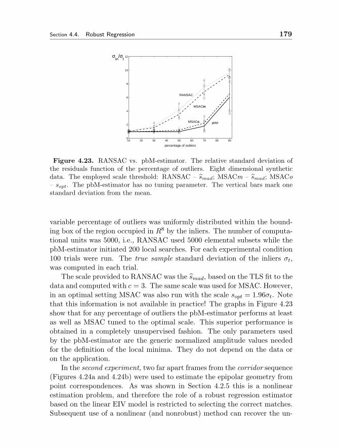
Section 4.4. Robust Regression 179
10 20 30 40 50 60 70 80 900
2
4
6
8
10
12
percentage of outliers
σin
/σt
pbMMSACo
MSACm
RANSAC
Figure 4.23. RANSAC vs. pbM-estimator. The relative standard deviation ofthe residuals function of the percentage of outliers. Eight dimensional syntheticdata. The employed scale threshold: RANSAC – smad; MSACm – smad; MSACo– sopt. The pbM-estimator has no tuning parameter. The vertical bars mark onestandard deviation from the mean.
variable percentage of outliers was uniformly distributed within the bound-ing box of the region occupied in R8 by the inliers. The number of computa-tional units was 5000, i.e., RANSAC used 5000 elemental subsets while thepbM-estimator initiated 200 local searches. For each experimental condition100 trials were run. The true sample standard deviation of the inliers σt,was computed in each trial.
The scale provided to RANSAC was the smad, based on the TLS fit to thedata and computed with c = 3. The same scale was used for MSAC. However,in an optimal setting MSAC was also run with the scale sopt = 1.96σt. Notethat this information is not available in practice! The graphs in Figure 4.23show that for any percentage of outliers the pbM-estimator performs at leastas well as MSAC tuned to the optimal scale. This superior performance isobtained in a completely unsupervised fashion. The only parameters usedby the pbM-estimator are the generic normalized amplitude values neededfor the definition of the local minima. They do not depend on the data oron the application.
In the second experiment, two far apart frames from the corridor sequence(Figures 4.24a and 4.24b) were used to estimate the epipolar geometry frompoint correspondences. As was shown in Section 4.2.5 this is a nonlinearestimation problem, and therefore the role of a robust regression estimatorbased on the linear EIV model is restricted to selecting the correct matches.Subsequent use of a nonlinear (and nonrobust) method can recover the un-
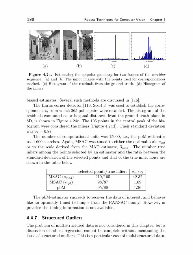
180 Robust Techniques for Computer Vision Chapter 4
−150 −100 −50 0 50 1000
10
20
30
40
50
60
70
80
90
100
residuals −3 −2 −1 0 1 2 3
0
2
4
6
8
10
12
14
16
18
inlier residuals
(a) (b) (c) (d)
Figure 4.24. Estimating the epipolar geometry for two frames of the corridorsequence. (a) and (b) The input images with the points used for correspondencesmarked. (c) Histogram of the residuals from the ground truth. (d) Histogram ofthe inliers.
biased estimates. Several such methods are discussed in [116].The Harris corner detector [110, Sec.4.3] was used to establish the corre-
spondences, from which 265 point pairs were retained. The histogram of theresiduals computed as orthogonal distances from the ground truth plane in8D, is shown in Figure 4.24c. The 105 points in the central peak of the his-togram were considered the inliers (Figure 4.24d). Their standard deviationwas σt = 0.88.
The number of computational units was 15000, i.e., the pbM-estimatorused 600 searches. Again, MSAC was tuned to either the optimal scale soptor to the scale derived from the MAD estimate, smad. The number trueinliers among the points selected by an estimator and the ratio between thestandard deviation of the selected points and that of the true inlier noise areshown in the table below.
selected points/true inliers σin/σtMSAC (smad) 219/105 42.32MSAC (sopt) 98/87 1.69
pbM 95/88 1.36
The pbM-estimator succeeds to recover the data of interest, and behaveslike an optimally tuned technique from the RANSAC family. However, inpractice the tuning information is not available.
4.4.7 Structured Outliers
The problem of multistructured data is not considered in this chapter, but adiscussion of robust regression cannot be complete without mentioning theissue of structured outliers. This is a particular case of multistructured data,
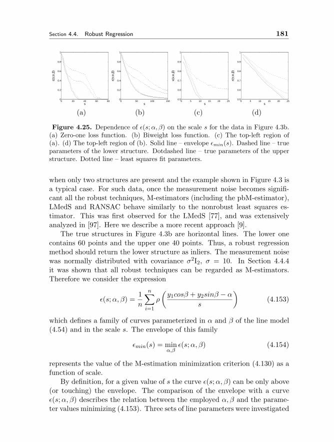
Section 4.4. Robust Regression 181
0 20 40 60 800
0.2
0.4
0.6
0.8
1
s
ε(s;
α,β)
0 50 100 1500
0.2
0.4
0.6
0.8
1
s
ε(s;
α,β)
0 5 10 15 20 250.5
0.6
0.7
0.8
0.9
1
s
ε(s;
α,β)
0 5 10 15 20 250.5
0.6
0.7
0.8
0.9
1
s
ε(s;
α,β)
(a) (b) (c) (d)
Figure 4.25. Dependence of ε(s;α, β) on the scale s for the data in Figure 4.3b.(a) Zero-one loss function. (b) Biweight loss function. (c) The top-left region of(a). (d) The top-left region of (b). Solid line – envelope εmin(s). Dashed line – trueparameters of the lower structure. Dotdashed line – true parameters of the upperstructure. Dotted line – least squares fit parameters.
when only two structures are present and the example shown in Figure 4.3 isa typical case. For such data, once the measurement noise becomes signifi-cant all the robust techniques, M-estimators (including the pbM-estimator),LMedS and RANSAC behave similarly to the nonrobust least squares es-timator. This was first observed for the LMedS [77], and was extensivelyanalyzed in [97]. Here we describe a more recent approach [9].
The true structures in Figure 4.3b are horizontal lines. The lower onecontains 60 points and the upper one 40 points. Thus, a robust regressionmethod should return the lower structure as inliers. The measurement noisewas normally distributed with covariance σ2I2, σ = 10. In Section 4.4.4it was shown that all robust techniques can be regarded as M-estimators.Therefore we consider the expression
ε(s;α, β) =1n
n∑i=1
ρ
(y1cosβ + y2sinβ − α
s
)(4.153)
which defines a family of curves parameterized in α and β of the line model(4.54) and in the scale s. The envelope of this family
εmin(s) = minα,β
ε(s;α, β) (4.154)
represents the value of the M-estimation minimization criterion (4.130) as afunction of scale.
By definition, for a given value of s the curve ε(s;α, β) can be only above(or touching) the envelope. The comparison of the envelope with a curveε(s;α, β) describes the relation between the employed α, β and the parame-ter values minimizing (4.153). Three sets of line parameters were investigated
182 Robust Techniques for Computer Vision Chapter 4
using the zero-one (Figure 4.25a) and the biweigth (Figure 4.25b) loss func-tions: the true parameters of the two structures (α = 50, 100;β = π/2), andthe least squares parameter estimates (αLS , βLS). The LS parameters yielda line similar to the one in Figure 4.3b, a nonrobust result.
Consider the case of zero-one loss function and the parameters of thelower structure (dashed line in Figure 4.25a). For this loss function ε(s; 50, π/2)is the percentage of data points outside the horizontal band centered ony2 = 50 and with half-width s. As expected the curve has a plateau aroundε = 0.4 corresponding to the band having one of its boundaries in thetransition region between the two structures. Once the band extends intothe second structure ε(s; 50, π/2) further decreases. The curve, however, isnot only always above the envelope, but most often also above the curveε(s;αLS , βLS). See the magnified area of small scales in Figure 4.25c.
For a given value of the scale (as in RANSAC) a fit similar to least squareswill be prefered since it yields a smaller value for (4.153). The measurementnoise being large, a band containing half the data (as in LMedS) correspondsto a scale s > 12, the value around which the least squares fit begins todominate the optimization (Figure 4.25a). As a result the LMedS will alwaysfail (Figure 4.3b). Note also the very narrow range of scale values (around s =10) for which ε(s; 50, π/2) is below ε(s;αLS , βLS). It shows how accuratelyhas the user to tune an estimator in the RANSAC family for a satisfactoryperformance.
The behavior for the biweight loss function is identical, only the curvesare smoother due to the weigthed averages (Figures 4.25b and 4.25d). Whenthe noise corrupting the structures is small, in Figure 4.3a it is σ = 2, theenvelope and the curve ε(s; 50, π/2) overlap for s < 8 which suffices for theLMedS criterion. See [9] for details.
We can conclude that multistructured data has to be processed first bybreaking it into parts in which one structure dominates. The technique in [8]combines several of the procedures discussed in this chapter. The samplingwas guided by local data density, i.e., it was assumed that the structures andthe background can be roughly separated by a global threshold on nearestneighbor distances. The pbM-estimator was employed as the estimationmodule, and the final parameters were obtained by applying adaptive meanshift to a feature space. The technique had a Hough transform flavor, thoughno scale parameters were required. The density assumption, however, mayfail when the structures are defined by linearizing a nonlinear problem, as itis often the case in 3D vision. Handling such multistructured data embeddedin a significant background clutter, remains an open question.
Section 4.5. Conclusion 183
4.5 Conclusion
Our goal in this chapter was to approach robust estimation from the pointof view of a practitioner. We have used a common statistical frameworkwith solid theoretical foundations to discuss the different types and classesof robust estimators. Therefore, we did not dwell on techniques which havean excellent robust behavior but are of a somewhat ad-hoc nature. Thesetechniques, such as tensor voting (see Chapter 5), can provide valuable toolsfor solving difficult computer vision problems.
Another disregarded topic was the issue of diagnosis. Should an algo-rithm be able to determine its own failure, one can already talk about robustbehavior. When in the late 1980’s robust methods became popular in thevision community, the paper [28] was often considered as the first robustwork in the vision literature. The special issue [93] and the book [6] containrepresentative collections of papers for the state-of-the-art today.
We have emphasized the importance of embedding into the employedmodel the least possible amount of assumptions necessary for the task athand. In this way the developed algorithms are more suitable for visionapplications, where the data is often more complex than in the statisticalliterature. However, there is a tradeoff to satisfy. As the model becomesless committed (more nonparametric), its power to extrapolate from theavailable data also decreases. How much is modeled rigorously and howmuch is purely data driven is an important decision of the designer of analgorithm. The material presented in this chapter was intended to help intaking this decision.
Acknowledgements
I must thank to several of my current and former graduate students whosework is directly or indirectly present on every page: Haifeng Chen, DorinComaniciu, Bogdan Georgescu, Yoram Leedan and Bogdan Matei. Long dis-cussions with Dave Tyler from the Statistics Department, Rutgers Universityhelped to crystallize many of the ideas described in this paper. Should theybe mistaken, the blame is entirely mine. Preparation of the material was sup-ported by the National Science Foundation under the grant IRI 99-87695.
Bibliography
[1] J. Addison. Pleasures of imagination. Spectator, 6, No. 411, June 21, 1712.[2] G. Antille and H. El May. The use of slices in the LMS and the method of
density slices: Foundation and comparison. In Y. Dodge and J. Whittaker,
184 Robust Techniques for Computer Vision Chapter 4
editors, Proc. 10th Symp. Computat. Statist., Neuchatel, volume I, pages 441–445. Physica-Verlag, 1992.
[3] T. Arbel and F. P. Ferrie. On sequential accumulation of evidence. Intl. J. ofComputer Vision, 43:205–230, 2001.
[4] P. J. Besl, J. B. Birch, and L. T. Watson. Robust window operators. InProceedings of the 2nd International Conference on Computer Vision, pages591–600, Tampa, FL, December 1988.
[5] M.J. Black and A. Rangarajan. On the unification of line processes, outlierrejection, and robust statistics with applications in early vision. Intl. J. ofComputer Vision, 19:57–91, 1996.
[6] K. J. Bowyer and P. J. Phillips, editors. Empirical evaluation techniques incomputer vision. IEEE Computer Society, 1998.
[7] K. L. Boyer, M. J. Mirza, and G. Ganguly. The robust sequential estimator:A general approach and its application to surface organization in range data.IEEE Trans. Pattern Anal. Machine Intell., 16:987–1001, 1994.
[8] H. Chen and P. Meer. Robust computer vision through kernel density estima-tion. In Proc. European Conf. on Computer Vision, Copenhagen, Denmark,volume I, pages 236–250, May 2002.
[9] H. Chen, P. Meer, and D. E. Tyler. Robust regression for data with multi-ple structures. In 2001 IEEE Conference on Computer Vision and PatternRecognition, volume I, pages 1069–1075, Kauai, HI, December 2001.
[10] Y. Cheng. Mean shift, mode seeking, and clustering. IEEE Trans. PatternAnal. Machine Intell., 17:790–799, 1995.
[11] E. Choi and P. Hall. Data sharpening as a prelude to density estimation.Biometrika, 86:941–947, 1999.
[12] W. Chojnacki, M. J. Brooks, A. van den Hengel, and D. Gawley. On thefitting of surfaces to data with covariances. IEEE Trans. Pattern Anal. MachineIntell., 22:1294–1303, 2000.
[13] C.M. Christoudias, B. Georgescu, and P. Meer. Synergism in low-level vision.In Proc. 16th International Conference on Pattern Recognition, Quebec City,Canada, volume IV, pages 150–155, August 2002.
[14] R. T. Collins. Mean-shift blob tracking through scale space. In Proc. IEEEConf. on Computer Vision and Pattern Recognition, Madison, WI, volume II,pages 234–240, 2003.
[15] D. Comaniciu. An algorithm for data-driven bandwidth selection. IEEE Trans.Pattern Anal. Machine Intell., 25:281–288, 2003.
[16] D. Comaniciu and P. Meer. Distribution free decomposition of multivariatedata. Pattern Analysis and Applications, 2:22–30, 1999.
[17] D. Comaniciu and P. Meer. Mean shift: A robust approach toward featurespace analysis. IEEE Trans. Pattern Anal. Machine Intell., 24:603–619, 2002.
[18] D. Comaniciu, V. Ramesh, and P. Meer. The variable bandwidth mean shiftand data-driven scale selection. In Proc. 8th Intl. Conf. on Computer Vision,Vancouver, Canada, volume I, pages 438–445, July 2001.
[19] D. Comaniciu, V. Ramesh, and P. Meer. Kernel-based object tracking. IEEETrans. Pattern Anal. Machine Intell., 25:564–577, 2003.
Bibliography 185
[20] D. Donoho, I. Johnstone, P. Rousseeuw, and W. Stahel. Discussion: Projectionpursuit. Annals of Statistics, 13:496–500, 1985.
[21] R.O. Duda, P.E. Hart, and D.G. Stork. Pattern Classification. Wiley, secondedition, 2001.
[22] B. Efron and R. Tibshirani. An Introduction to the Bootstrap. Chapman &Hall, New York, 1993.
[23] S. P. Ellis. Instability of least squares, least absolute deviation and least medianof squares linear regression. Statistical Science, 13:337–350, 1998.
[24] O. Faugeras. Three-Dimensional Computer Vision. MIT Press, 1993.[25] M.A. Fischler and R.C. Bolles. Random sample consensus: A paradigm for
model fitting with applications to image analysis and automated cartography. InDARPA Image Understanding Workshop, pages 71–88, University of Maryland,College Park, April 1980.
[26] M.A. Fischler and R.C. Bolles. Random sample consensus: A paradigm formodel fitting with applications to image analysis and automated cartography.Comm. Assoc. Comp. Mach, 24(6):381–395, 1981.
[27] A.W. Fitzgibbon, M. Pilu, and R.B. Fisher. Direct least square fitting of el-lipses. IEEE Trans. Pattern Anal. Machine Intell., 21:476–480, 1999.
[28] W. Forstner. Reliability analysis of parameter estimation in linear models withapplications to mensuration problems in computer vision. Computer Vision,Graphics, and Image Processing, 40:273–310, 1987.
[29] W. T. Freeman, E. G. Pasztor, and O. W. Carmichael. Learning in low-levelvision. Intl. J. of Computer Vision, 40:25–47, 2000.
[30] J. H. Friedman and J. W. Tukey. A projection pursuit algorithm for exploratorydata analysis. IEEE Trans. Comput., 23:881–889, 1974.
[31] K. Fukunaga. Introduction to Statistical Pattern Recognition. Academic Press,second edition, 1990.
[32] K. Fukunaga and L. D. Hostetler. The estimation of the gradient of a densityfunction, with applications in pattern recognition. IEEE Trans. InformationTheory, 21:32–40, 1975.
[33] W. Fuller. Measurement Error Models. Wiley, 1987.[34] B. Georgescu and P. Meer. Balanced recovery of 3D structure and camera mo-
tion from uncalibrated image sequences. In Proc. European Conf. on ComputerVision, Copenhagen, Denmark, volume II, pages 294–308, 2002.
[35] B. Georgescu, I. Shimshoni, and P. Meer. Mean shift based clustering in highdimensions: A texture classification example. In Proc. 9th Intl. Conf. on Com-puter Vision, Nice, France, pages 456–463, October 2003.
[36] E. B. Goldstein. Sensation and Perception. Wadsworth Publishing Co., 2ndedition, 1987.
[37] G. H. Golub and C. Reinsch. Singular value decomposition and least squaressolutions. Number. Math., 14:403–420, 1970.
[38] G. H. Golub and C. F. Van Loan. Matrix Computations. John Hopkins U.Press, second edition, 1989.
[39] P. Hall, T.C. Hui, and J.S. Marron. Improved variable window kernel estimatesof probability densities. Annals of Statistics, 23:1–10, 1995.
186 Robust Techniques for Computer Vision Chapter 4
[40] R. Hampel, E.M. Ronchetti, P.J. Rousseeuw, and W.A. Stahel. Robust Statis-tics. The Approach Based on Influence Function. Wiley, 1986.
[41] R. M. Haralick and H. Joo. 2D-3D pose estimation. In Proceedings of the 9thInternational Conference on Pattern Recognition, pages 385–391, Rome, Italy,November 1988.
[42] R. M. Haralick and L. G. Shapiro. Computer and Robot Vision. Addison-Wesley, 1992.
[43] R. Hartley and A. Zisserman. Multiple View Geometry in Computer Vision.Cambridge University Press, 2000.
[44] T. Hastie, R. Tibshirani, and J. Friedman. The Elements of Statistical Learning.Springer, 2001.
[45] T. P. Hettmansperger and S. J. Sheather. A cautionary note on the method ofleast median of squares. The American Statistician, 46:79–83, 1992.
[46] P.V.C. Hough. Machine analysis of bubble chamber pictures. In Interna-tional Conference on High Energy Accelerators and Instrumentation, CentreEuropeenne pour la Recherch Nucleaire (CERN), 1959.
[47] P.V.C. Hough. Method and means for recognizing complex patterns. US Patent3,069,654, December 18, 1962.
[48] P. J. Huber. Projection pursuit (with discussion). Annals of Statistics, 13:435–525, 1985.
[49] P. J. Huber. Robust Statistical Procedures. SIAM, second edition, 1996.[50] J. Illingworth and J. V. Kittler. A survey of the Hough transform. Computer
Vision, Graphics, and Image Processing, 44:87–116, 1988.[51] M. Isard and A. Blake. Condensation - Conditional density propagation for
visual tracking. Intl. J. of Computer Vision, 29:5–28, 1998.[52] A. K. Jain and R. C. Dubes. Algorithms for Clustering Data. Prentice Hall,
1988.[53] J.M. Jolion, P. Meer, and S. Bataouche. Robust clustering with applications
in computer vision. IEEE Trans. Pattern Anal. Machine Intell., 13:791–802,1991.
[54] M. C. Jones and R. Sibson. What is projection pursuit? (with discussion). J.Royal Stat. Soc. A, 150:1–37, 1987.
[55] B. Julesz. Early vision and focal attention. Rev. of Modern Physics, 63:735–772,1991.
[56] H. Kalviainen, P. Hirvonen, L. Xu, and E. Oja. Probabilistic and nonprob-abilistic Hough transforms: Overview and comparisons. Image and VisionComputing, 13:239–252, 1995.
[57] K. Kanatani. Statistical bias of conic fitting and renormalization. IEEE Trans.Pattern Anal. Machine Intell., 16:320–326, 1994.
[58] K. Kanatani. Statistical Optimization for Geometric Computation: Theory andPractice. Elsevier, 1996.
[59] D.Y. Kim, J.J. Kim, P. Meer, D. Mintz, and A. Rosenfeld. Robust computervision: The least median of squares approach. In Proceedings 1989 DARPAImage Understanding Workshop, pages 1117–1134, Palo Alto, CA, May 1989.
[60] N. Kiryati and A. M. Bruckstein. What’s in a set of points? IEEE Trans.Pattern Anal. Machine Intell., 14:496–500, 1992.
Bibliography 187
[61] N. Kiryati and A. M. Bruckstein. Heteroscedastic Hough transform (HtHT): Anefficient method for robust line fitting in the ‘errors in the variables’ problem.Computer Vision and Image Understanding, 78:69–83, 2000.
[62] V. F. Leavers. Survey: Which Hough transform? Computer Vision, Graphics,and Image Processing, 58:250–264, 1993.
[63] K.M. Lee, P. Meer, and R.H. Park. Robust adaptive segmentation of rangeimages. IEEE Trans. Pattern Anal. Machine Intell., 20:200–205, 1998.
[64] Y. Leedan and P. Meer. Heteroscedastic regression in computer vision: Prob-lems with bilinear constraint. Intl. J. of Computer Vision, 37:127–150, 2000.
[65] A. Leonardis and H. Bischof. Robust recognition using eigenimages. ComputerVision and Image Understanding, 78:99–118, 2000.
[66] R. M. Lewis, V. Torczon, and M. W. Trosset. Direct search methods: Thenand now. J. Computational and Applied Math., 124:191–207, 2000.
[67] G. Li. Robust regression. In D. C. Hoaglin, F. Mosteller, and J. W. Tukey, ed-itors, Exploring Data Tables, Trends, and Shapes, pages 281–343. Wiley, 1985.
[68] R. A. Maronna and V. J. Yohai. The breakdown point of simulataneous generalM estimates of regression and scale. J. of Amer. Stat. Assoc., 86:699–703, 1991.
[69] R. D. Martin, V. J. Yohai, and R. H. Zamar. Min-max bias robust regression.Annals of Statistics, 17:1608–1630, 1989.
[70] B. Matei. Heteroscedastic Errors-in-Variables Models in Com-puter Vision. PhD thesis, Department of Electrical and Com-puter Engineering, Rutgers University, 2001. Available athttp://www.caip.rutgers.edu/riul/research/theses.html.
[71] B. Matei and P. Meer. Bootstrapping errors-in-variables models. In B. Triggs,A. Zisserman, and R. Szelisky, editors, Vision Algorithms: Theory and Practice,pages 236–252. Springer, 2000.
[72] B. Matei and P. Meer. Reduction of bias in maximum likelihood ellipse fitting.In 15th International Conference on Computer Vision and Pattern Recog., vol-ume III, pages 802–806, Barcelona, Spain, September 2000.
[73] P. Meer and B. Georgescu. Edge detection with embedded confidence. IEEETrans. Pattern Anal. Machine Intell., 23:1351–1365, 2001.
[74] P. Meer, D. Mintz, D. Y. Kim, and A. Rosenfeld. Robust regression methodsin computer vision: A review. Intl. J. of Computer Vision, 6:59–70, 1991.
[75] J. M. Mendel. Lessons in Estimation Theory for Signal Processing, Communi-cations, and Control. Prentice Hall, 1995.
[76] J. V. Miller and C. V. Stewart. MUSE: Robust surface fitting using unbiasedscale estimates. In CVPR96, pages 300–306, June 1996.
[77] D. Mintz, P. Meer, and A. Rosenfeld. Consensus by decomposition: A paradigmfor fast high breakdown point robust estimation. In Proceedings 1991 DARPAImage Understanding Workshop, pages 345–362, La Jolla, CA, January 1992.
[78] J. A. Nelder and R. Mead. A simplex method for function minimization. Com-puter Journal, 7:308–313, 1965.
[79] P. L. Palmer, J. Kittler, and M. Petrou. An optimizing line finder using aHough transform algorithm. Computer Vision and Image Understanding, 67:1–23, 1997.
188 Robust Techniques for Computer Vision Chapter 4
[80] D. Petkovic, W. Niblack, and M. Flickner. Projection-based high accuracymeasurement of straight line edges. Machine Vision and Appl., 1:183–199,1988.
[81] P. D. Picton. Hough transform references. Internat. J. of Patt. Rec and Artific.Intell., 1:413–425, 1987.
[82] W. H. Press, S. A. Teukolsky, W. T. Vetterling, and B. P. Flannery. NumericalRecipes in C. Cambridge University Press, second edition, 1992.
[83] P. Pritchett and A. Zisserman. Wide baseline stereo matching. In 6th Interna-tional Conference on Computer Vision, pages 754–760, Bombay, India, January1998.
[84] Z. Pylyshyn. Is vision continuous with cognition? The case for cognitive im-penetrability of visual perception. Behavioral and Brain Sciences, 22:341–423,1999. (with comments).
[85] S.J. Raudys and A.K. Jain. Small sample size effects in statistical patternrecognition: Recommendations for practitioners. IEEE Trans. Pattern Anal.Machine Intell., 13:252–264, 1991.
[86] P. J. Rousseeuw. Least median of squares regression. J. of Amer. Stat. Assoc.,79:871–880, 1984.
[87] P. J. Rousseeuw. Unconventional features of positive-breakdown estimators.Statistics & Prob. Letters, 19:417–431, 1994.
[88] P. J. Rousseeuw and C. Croux. Alternatives to the median absolute deviation.J. of Amer. Stat. Assoc., 88:1273–1283, 1993.
[89] P. J. Rousseeuw and A. M. Leroy. Robust Regression and Outlier Detection.Wiley, 1987.
[90] D. Ruppert and D. G. Simpson. Comment on “Unmasking Multivariate Outliersand Leverage Points”, by P. J. Rousseeuw and B. C. van Zomeren. J. of Amer.Stat. Assoc., 85:644–646, 1990.
[91] D. W. Scott. Parametric statistical modeling by minimum integrated squareerror. Technometrics, 43:247–285, 2001.
[92] B. W. Silverman. Density Estimation for Statistics and Data Analysis. Chap-man & Hall, 1986.
[93] Special Issue. Performance evaluation. Machine Vision and Appl., 9(5/6), 1997.[94] Special Issue. Robust statistical techniques in image understanding. Computer
Vision and Image Understanding, 78, April 2000.[95] G. Speyer and M. Werman. Parameter estimates for a pencil of lines: Bounds
and estimators. In Proc. European Conf. on Computer Vision, Copenhagen,Denmark, volume I, pages 432–446, 2002.
[96] L. Stark and K.W. Bowyer. Achieving generalized object recognition throughreasoning about association of function to structure. IEEE Trans. Pattern Anal.Machine Intell., 13:1097–1104, 1991.
[97] C. V. Stewart. Bias in robust estimation caused by discontinuities and multiplestructures. IEEE Trans. Pattern Anal. Machine Intell., 19:818–833, 1997.
[98] C. V. Stewart. Robust parameter estimation in computer vision. SIAM Reviews,41:513–537, 1999.
[99] C.V. Stewart. Minpran: A new robust estimator for computer vision. IEEETrans. Pattern Anal. Machine Intell., 17:925–938, 1995.
Bibliography 189
[100] K. S. Tatsuoka and D. E. Tyler. On the uniqueness of S and constrainedM-functionals under non-elliptical distributions. Annals of Statistics, 28:1219–1243, 2000.
[101] P. R. Thrift and S. M. Dunn. Approximating point-set images by line segmentsusing a variation of the Hough transform. Computer Vision, Graphics, andImage Processing, 21:383–394, 1983.
[102] A. Tirumalai and B. G. Schunk. Robust surface approximation using least me-dian of squares. Technical Report CSE-TR-13-89, Artificial Intelligence Labo-ratory, 1988. University of Michigan, Ann Arbor.
[103] B. Tordoff and D.W. Murray. Guided sampling and consensus for motionestimation. In 7th European Conference on Computer Vision, volume I, pages82–96, Copenhagen, Denmark, May 2002.
[104] P. H. S. Torr and C. Davidson. IMPSAC: Synthesis of importance samplingand random sample consensus. IEEE Trans. Pattern Anal. Machine Intell.,25:354–364, 2003.
[105] P. H. S. Torr and D. W. Murray. The development and comparison of robustmethods for estimating the fundamental matrix. Intl. J. of Computer Vision,24:271–300, 1997.
[106] P. H. S. Torr and A. Zisserman. MLESAC: A new robust estimator withapplication to estimating image geometry. Computer Vision and Image Under-standing, 78:138–156, 2000.
[107] P. H. S. Torr, A. Zisserman, and S. J. Maybank. Robust detection of degenerateconfigurations while estimating the fundamental matrix. Computer Vision andImage Understanding, 71:312–333, 1998.
[108] P.H.S. Torr and A. Zisserman. Robust computation and parametrization ofmultiple view relations. In 6th International Conference on Computer Vision,pages 727–732, Bombay, India, January 1998.
[109] A. Treisman. Features and objects in visual processing. Scientific American,254:114–125, 1986.
[110] E. Trucco and A. Verri. Introductory Techniques for 3-D Computer Vision.Prentice Hall, 1998.
[111] S. Van Huffel and J. Vandewalle. The Total Least Squares Problem. Computa-tional Aspects and Analysis. Society for Industrial and Applied Mathematics,1991.
[112] M. P. Wand and M.C. Jones. Kernel Smoothing. Chapman & Hall, 1995.[113] I. Weiss. Line fitting in a noisy image. IEEE Trans. Pattern Anal. Machine
Intell., 11:325–329, 1989.[114] M. H. Wright. Direct search methods: Once scorned, now respectable. In D. H.
Griffiths and G. A. Watson, editors, Numerical Analysis 1995, pages 191–208.Addison-Wesley Longman, 1996.
[115] R. H. Zamar. Robust estimation in the errors-in-variables model. Biometrika,76:149–160, 1989.
[116] Z. Zhang. Determining the epipolar geometry and its uncertainty: A review.Intl. J. of Computer Vision, 27:161–195, 1998.
[117] Z. Zhang. Parameter-estimation techniques: A tutorial with application toconic fitting. Image and Vision Computing, 15:59–76, 1997.

Chapter 5
THE TENSOR VOTINGFRAMEWORK
Gerard Medioni
and Philippos Mordohai
5.1 Introduction
The design and implementation of a complete artificial vision system is adaunting challenge. The computer vision community has made significantprogress in many areas, but the ultimate goal is still far-off. A key componentof a general computer vision system is a computational framework that canaddress a wide range of problems in a unified way. We have developedsuch a framework over the past several years [40], which is the basis of theaugmented framework that is presented in this chapter. It is based on a datarepresentation formalism that uses tensors and an information propagationmechanism termed tensor voting.
Most computer vision problems are inverse problems, due to the factthat the imaging process maps 3-D “world” features onto 2-D arrays of pix-els. The loss of information due to the reduction in dimensionality and thefact the imaging process is not linear combined with unavoidable sourcesof noise, such as limited sensor resolution, quantization of continuous in-formation into pixels, photometric and projective distortion, guarantee thatcomputer vision algorithms operate on datasets that include numerous out-liers and are severely corrupted by noise. Many scene configurations couldhave generated a given image (see Fig. 5.1). An automated computer visionsystem must impose constraints or prior knowledge about the appearance
191
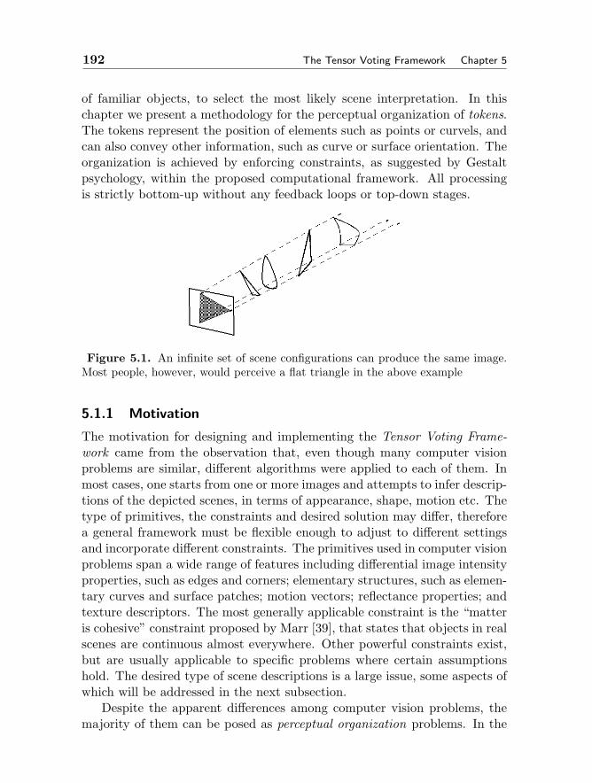
192 The Tensor Voting Framework Chapter 5
of familiar objects, to select the most likely scene interpretation. In thischapter we present a methodology for the perceptual organization of tokens.The tokens represent the position of elements such as points or curvels, andcan also convey other information, such as curve or surface orientation. Theorganization is achieved by enforcing constraints, as suggested by Gestaltpsychology, within the proposed computational framework. All processingis strictly bottom-up without any feedback loops or top-down stages.
Figure 5.1. An infinite set of scene configurations can produce the same image.Most people, however, would perceive a flat triangle in the above example
5.1.1 Motivation
The motivation for designing and implementing the Tensor Voting Frame-work came from the observation that, even though many computer visionproblems are similar, different algorithms were applied to each of them. Inmost cases, one starts from one or more images and attempts to infer descrip-tions of the depicted scenes, in terms of appearance, shape, motion etc. Thetype of primitives, the constraints and desired solution may differ, thereforea general framework must be flexible enough to adjust to different settingsand incorporate different constraints. The primitives used in computer visionproblems span a wide range of features including differential image intensityproperties, such as edges and corners; elementary structures, such as elemen-tary curves and surface patches; motion vectors; reflectance properties; andtexture descriptors. The most generally applicable constraint is the “matteris cohesive” constraint proposed by Marr [39], that states that objects in realscenes are continuous almost everywhere. Other powerful constraints exist,but are usually applicable to specific problems where certain assumptionshold. The desired type of scene descriptions is a large issue, some aspects ofwhich will be addressed in the next subsection.
Despite the apparent differences among computer vision problems, themajority of them can be posed as perceptual organization problems. In the
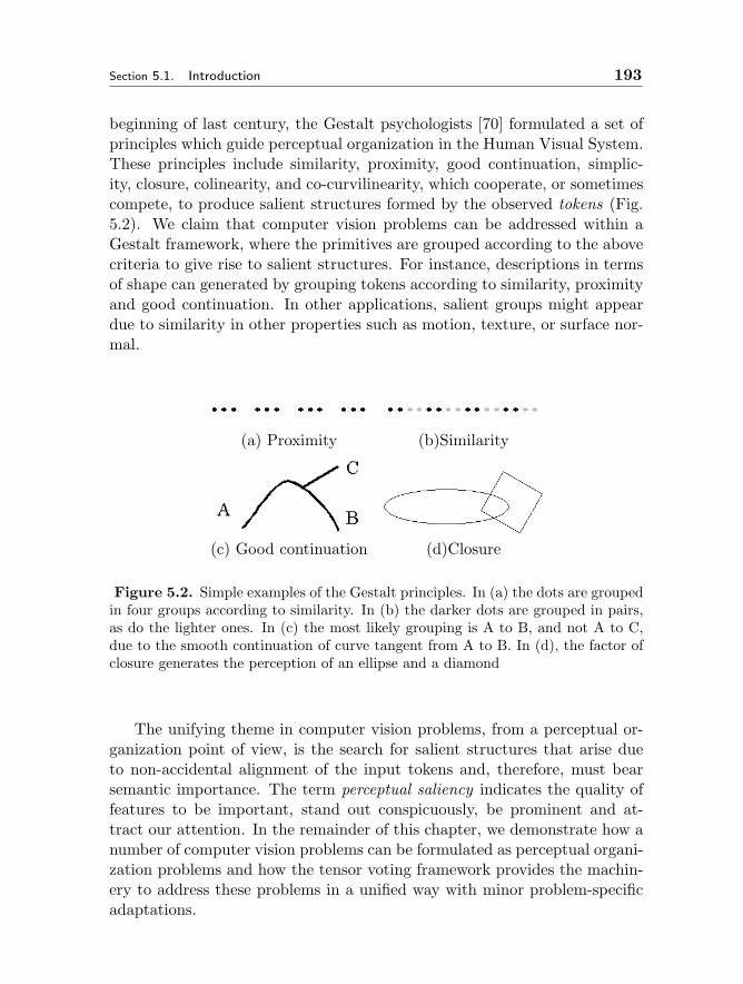
Section 5.1. Introduction 193
beginning of last century, the Gestalt psychologists [70] formulated a set ofprinciples which guide perceptual organization in the Human Visual System.These principles include similarity, proximity, good continuation, simplic-ity, closure, colinearity, and co-curvilinearity, which cooperate, or sometimescompete, to produce salient structures formed by the observed tokens (Fig.5.2). We claim that computer vision problems can be addressed within aGestalt framework, where the primitives are grouped according to the abovecriteria to give rise to salient structures. For instance, descriptions in termsof shape can generated by grouping tokens according to similarity, proximityand good continuation. In other applications, salient groups might appeardue to similarity in other properties such as motion, texture, or surface nor-mal.
(a) Proximity (b)Similarity
(c) Good continuation (d)Closure
Figure 5.2. Simple examples of the Gestalt principles. In (a) the dots are groupedin four groups according to similarity. In (b) the darker dots are grouped in pairs,as do the lighter ones. In (c) the most likely grouping is A to B, and not A to C,due to the smooth continuation of curve tangent from A to B. In (d), the factor ofclosure generates the perception of an ellipse and a diamond
The unifying theme in computer vision problems, from a perceptual or-ganization point of view, is the search for salient structures that arise dueto non-accidental alignment of the input tokens and, therefore, must bearsemantic importance. The term perceptual saliency indicates the quality offeatures to be important, stand out conspicuously, be prominent and at-tract our attention. In the remainder of this chapter, we demonstrate how anumber of computer vision problems can be formulated as perceptual organi-zation problems and how the tensor voting framework provides the machin-ery to address these problems in a unified way with minor problem-specificadaptations.
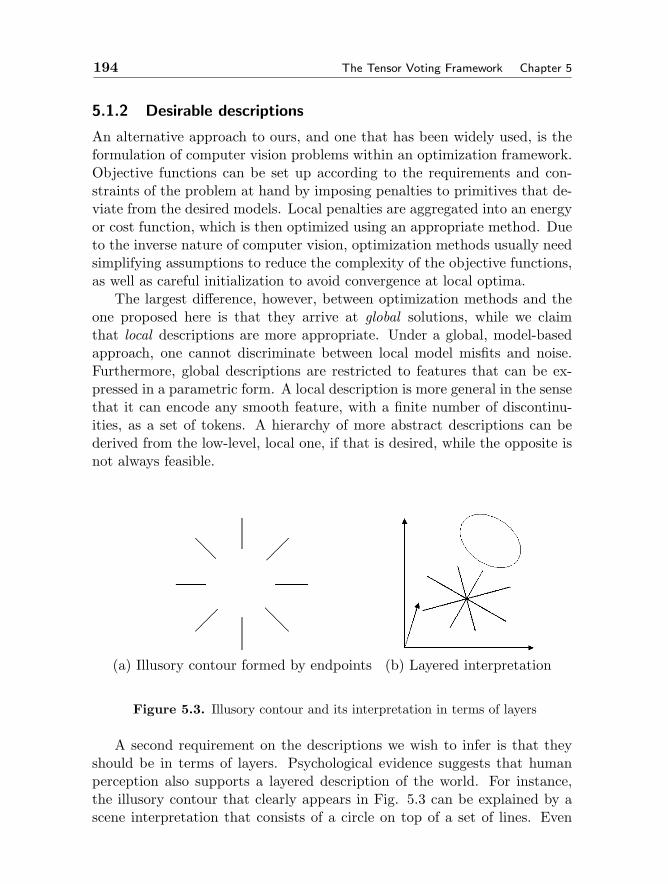
194 The Tensor Voting Framework Chapter 5
5.1.2 Desirable descriptions
An alternative approach to ours, and one that has been widely used, is theformulation of computer vision problems within an optimization framework.Objective functions can be set up according to the requirements and con-straints of the problem at hand by imposing penalties to primitives that de-viate from the desired models. Local penalties are aggregated into an energyor cost function, which is then optimized using an appropriate method. Dueto the inverse nature of computer vision, optimization methods usually needsimplifying assumptions to reduce the complexity of the objective functions,as well as careful initialization to avoid convergence at local optima.
The largest difference, however, between optimization methods and theone proposed here is that they arrive at global solutions, while we claimthat local descriptions are more appropriate. Under a global, model-basedapproach, one cannot discriminate between local model misfits and noise.Furthermore, global descriptions are restricted to features that can be ex-pressed in a parametric form. A local description is more general in the sensethat it can encode any smooth feature, with a finite number of discontinu-ities, as a set of tokens. A hierarchy of more abstract descriptions can bederived from the low-level, local one, if that is desired, while the opposite isnot always feasible.
(a) Illusory contour formed by endpoints (b) Layered interpretation
Figure 5.3. Illusory contour and its interpretation in terms of layers
A second requirement on the descriptions we wish to infer is that theyshould be in terms of layers. Psychological evidence suggests that humanperception also supports a layered description of the world. For instance,the illusory contour that clearly appears in Fig. 5.3 can be explained by ascene interpretation that consists of a circle on top of a set of lines. Even
Section 5.1. Introduction 195
though we do not aim to emulate the human visual system, this evidencesuggests that a layered representation is beneficial for a general computervision system.
Finally, we choose an object-based representation over a viewpoint-basedone. With this choice we avoid introducing unnecessary viewpoint-dependantelements in intermediate stages of the computation. For instance, if unique-ness along the lines of sight is a reasonable or desired assumption for a givenproblem, it can be enforced at later stages, thus avoiding the enforcement ofconstraints too early, when they might be detrimental to the solution.
5.1.3 Our approach
In this section we briefly review the tensor voting framework, which wasoriginally presented in [40], including extensions that have been developedin the past few years. The two main aspects of the framework are the repre-sentation by tensors and the information propagation mechanism by tensorvoting. Its purpose is to serve as a computational mechanism for perceptualgrouping of oriented and un-oriented tokens generated based on image orother primitives. It has mainly been applied to mid-level vision problems,but it is suitable for any problem, of any dimensionality, that can be formu-lated as a perceptual organization problem. The novelty of our approach isthat there is no objective function that is explicitly defined and optimized ac-cording to global criteria. Instead, tensor voting is performed locally and thesaliency of perceptual structures is estimated as a function of the supporttokens receive from their neighbors. Tokens with compatible orientationsthat can form salient structures reinforce each other. The support of a tokenfor its neighbors is expressed by votes that are cast according to the Gestaltprinciples of proximity, co-linearity and co-curvilinearity.
Data representation The representation of a token originally consisted of asymmetric second order tensor that encodes perceptual saliency. The tensoressentially indicates the saliency of each type of perceptual structure thetoken belongs to, and its preferred normal or tangent orientations. Tensorswere first used as a signal processing tool for computer vision applicationsby Granlund and Knutsson [12] and Westin [71]. Our use of tensors differsin that our representation is not signal based, but rather symbolic, wherehypotheses for the presence of a perceptual structure at a given location arerepresented as tokens with associated second order tensors that encode themost likely type of structure and its preferred tangent or normal orientations.The power of this representation lies in that all types of saliency are encodedby the same tensor.
196 The Tensor Voting Framework Chapter 5
The second order symmetric tensors fulfill the requirements set in theprevious paragraphs, since they are well suited as descriptors of local struc-ture. As opposed to scalar saliency values, the representation by tensors isricher in information, since it also encodes orientation hypotheses at eachlocation, thus allowing the application of Gestalt principles such as goodcontinuation, colinearity and co-curvilinearity. Even though this is also fea-sible with vectors, as in the work of Guy and Medioni [15, 16], the tensorscan simultaneously encode all potential types of structures, such as surfaces,curves and regions, as well as the uncertainty of the information.
A representation scheme sufficient for our purposes must be able to en-code both smooth perceptual structures as well as discontinuities which comein two types: orientation and structural discontinuities. The former occurat locations where a perceptual structure is continuous, but its orientationis not, or where multiple salient structures, such as curves or surfaces, meet.Curve orientation discontinuities occur at locations where multiple curve seg-ments intersect, while surface orientation discontinuities occur where mul-tiple surface patches intersect. In other words, whereas there is only oneorientation associated with a location within a smooth curve segment, or asurface patch or a region boundary, there are multiple orientations associ-ated with locations where a discontinuity occurs. Hence, the desirable datarepresentation is the that can encode more than one orientation at a given lo-cation. It turns out that a second order symmetric tensor possesses preciselythis property, as will be shown in Sections 5.3 and 5.4.
The second type of discontinuities are structural discontinuities. Theseoccur at locations such as the endpoints B and C of Fig. 5.8(a). They arefirst order discontinuities since the perceptual structure is no longer con-tinuous there. Non-accidental terminations of perceptual structures carrysignificant weight and should be explicitly detected and represented. Thesecond order symmetric tensors fail to describe structural discontinuities be-cause they cannot capture first order properties and the second order prop-erties of the structure remain invariant at its boundaries. In order to addressthis shortcoming of the framework, as it was published in [40], vectors (firstorder tensors) were introduced [69]. More specifically, besides the secondorder tensor, each token is associated with a polarity vector that encodes thelikelihood of the token being a termination of a perceptual structure. Po-larity vectors are sensitive to first order properties such as the distributionof neighboring tokens around a given token. Structure terminations can bedetected based on their essential property to have all their neighbors, at leastlocally, on the same side of a half-space.
Section 5.1. Introduction 197
Tensor Voting The way to encode primitives in the representation schemeis demonstrated in the following sections. The starting point in our attemptto infer salient structures and scene descriptions is a set of un-oriented ororiented tokens. Un-oriented tokens express the hypothesis that a perceptualstructure, of an unknown yet type, exists at the token’s location. Orientedtokens can be elementary curves (curvels), elementary surfaces (surfels) etc.They express the hypothesis that a perceptual structure with the given ori-entation goes through the location of the token. The question is how shouldthese hypotheses be combined in order to derive the saliency of each token?
We propose to do this by tensor voting, a method of information propa-gation where tokens convey their orientation preferences to their neighborsin the form of votes. First and second order votes, which are respectivelyvectors and second order tensors, are cast from token to token. The secondorder vote is a second order tensor that has the orientation in terms of nor-mals and tangents the receiver would have if the voter and receiver were partof the same smooth perceptual structure. The first order vote is a vectorthat points towards the voter, and thus the interior of the structure, if thereceiver ware indeed a boundary.
Each vote is an estimate of orientation or termination of a perceptualstructure consisting of just two tokens: the voter and the receiver. Inessence, simple, smooth perceptual structures are fitted between the twolocations to generate the orientation estimates at the receiver. According tothe Gestalt principle of proximity, the strength of the votes attenuates withdistance, making the influence from distant tokens, and possible interferencefrom unrelated ones, smaller. The strength of the vote also decreases withincreased curvature of the hypothesized structure, making straight continu-ations preferable to curved ones following the principles of smooth continu-ation and simplicity.
A large number of first and second order votes are accumulated at eachlocation. By analyzing the consistency of the orientation estimations and theamount of support a token receives, we can determine the type of structurethat exists at the location and its saliency. The aggregation of support viatensor voting is a generalization to the Hough transform [23] that was firstproposed by Guy and Medioni [15, 16] using a vector-based scheme.
5.1.4 Chapter Overview
This chapter is organized as follows:
– Section 5.2 is a review of related work in perceptual organization.
– Section 5.3 presents the tensor voting framework in 2-D.

198 The Tensor Voting Framework Chapter 5
– Section 5.4 shows how it can be generalized to 3-D.
– Section 5.5 presents the N-D version of the framework and a compu-tational complexity analysis.
– Section 5.6 addresses how computer vision problems can be posedwithin the framework and presents our results on stereo and motionanalysis.
– Section 5.7 concludes the chapter after pointing out some issues thatstill remain open.
5.2 Related Work
Perceptual organization has been an active research area. Important issuesinclude noise robustness, initialization requirements, handling of disconti-nuities, flexibility in the types that can be represented, and computationalcomplexity. This section reviews related work which can be classified in thefollowing categories:
– regularization
– relaxation labeling
– computational geometry
– robust methods
– level set methods
– symbolic methods
– clustering
– methods based on local interactions
– methods inspired by psychophysiology and neuroscience.
Regularization Due to the projective nature of imaging, a single image cancorrespond to different scene configurations. This ambiguity in image for-mation makes the inverse problem, the inference of structures from images,ill-posed. To address ill-posed problems, constraints have to be imposedon the solution space. Within the regularization theory, this is achievedby selecting an appropriate objective function and optimizing it accordingto the constraints. Poggio, Torre and Koch [51] present the application of
Section 5.2. Related Work 199
regularization theory to computer vision problems. Terzopoulos [65], andRobert and Deriche [52] address the issue of preserving discontinuities whileenforcing global smoothness in a regularization framework. A Bayesian for-mulation of the problem based on Minimum Description Length is proposedby Leclerc [32]. Variational techniques are used by Horn and Schunk [22]for the estimation of optical flow, and by Morel and Solimini [43] for imagesegmentation. In both cases the goal is to infer functions that optimize theselected criteria, while preserving discontinuities.
Relaxation labeling A different approach to vision problems is relaxationlabeling. The problems are cast as the assignment of labels to the elementsof the scene from a set of possible labels. Haralick and Shapiro define theconsistent labeling problem in [17] and [18]. Labels that violate consistencyaccording to predefined criteria are iteratively removed from the tokens untilconvergence. Faugeras and Berthod [8] describe a gradient optimizationapproach to relaxation labeling. A global criterion is defined that combinesthe concepts of ambiguity and consistency of the labeling process. Gemanand Geman discuss how stochastic relaxation can be applied to the task ofimage restoration in [11]. MAP estimates are obtained by a Gibbs samplerand simulated annealing. Hummel and Zucker [24] develop an underlyingtheory for the continuous relaxation process. One result is the definition ofan explicit function to maximize to guide the relaxation process, leading toa new relaxation operator. The second result is that finding a consistentlabeling is equivalent to solving a variational inequality. This work wascontinued by Parent and Zucker [50] for the inference of trace points in 2-D,and by Sander and Zucker [54] in 3-D.
Computational geometry Techniques for inferring surfaces from 3-D pointclouds have been reported in the computer graphics literature. Boissonnat[2] proposes a technique based on computational geometry for object rep-resentation by triangulating point clouds in 3-D. Hoppe et al. [21] infersurfaces from unorganized point clouds as the zero levels of a signed dis-tance function from the unknown surface. The strength of their approachlies in the fact that the surface model, topology and boundaries need notbe known a priori. Later, Edelsbrunner and Mucke [7] introduce the three-dimensional alpha shapes that are based on a 3-D Delaunay triangulationof the data. Szeliski, Tonnesen and Terzopoulos [61] describe a methodfor modeling surfaces of arbitrary, or changing, topology using a set of ori-ented dynamic particles which interact according to distance, co-planarity,co-normality and co-circularity. Computational geometry methods are lim-ited by their sensitivity to even a very small number of outliers, and their

200 The Tensor Voting Framework Chapter 5
computational complexity.
Robust methods In the presence of noise, robust techniques inspired byRANSAC (random sample consensus) [9] can be applied. Small random sam-ples are selected from the noisy data and are used to derive model hypotheseswhich are tested using the remainder of the dataset. Hypotheses that areconsistent with a large number of the data points are considered valid. Vari-ants of RANSAC include RESC [74] and MIR [31], which are mainly usedfor segmentation of surfaces from noisy 3-D point clouds. The extractedsurfaces are limited to planar or quadratic, except for the approach in [33]which can extract high-order polynomial surfaces. Chen et al. [4] intro-duce robust statistical methods to computer vision. They show how robustM-estimators with auxiliary scale are more general than the other robustestimators previously used in the field. They also point out the difficultiescaused by multiple structures in the data and propose a way to detect them.In all cases an a priori parametric representation of the unknown structureis necessary, thus limiting the applicability of these methods.
Level set methods The antipode of the explicit representation of surfacesby a set of points, is the implicit representation in terms of a function.In [58], Sethian proposes a level set approach under which surfaces can beinferred as the zero-level iso-surface of a multivariate implicit function. Thetechnique allows for topological changes, thus it can reconstruct surfacesof any genus as well as non-manifolds. Zhao, Osher and Fedkiw [20] andOsher and Fedkiw [49] propose efficient ways of handling implicit surfacesas level sets of a function. A combination of points and elementary surfacesand curves can be provided as input to their technique, which can handlelocal changes locally, as well as global deformations and topological changes.All the implicit surface-based approaches are iterative and require carefulselection of the implicit function and initialization. The surface in explicitform, as a set of polygons, can be extracted by a technique such as theclassic Marching Cubes algorithm [37]. The simultaneous representation ofsurfaces, curves and junctions is impossible.
Symbolic methods Following the paradigm set by Marr [39], many researchersdeveloped methods for hierarchical grouping of symbolic data. Lowe [38] de-veloped a system for 3-D object recognition based on perceptual organizationof image edgels. Groupings are selected among the numerous possibilities ac-cording to the Gestalt principles, viewpoint invariance and low likelihood ofbeing accidental formations. Later, Mohan and Nevatia [41] and Dolan andRiseman [6] also propose perceptual organization approaches based on the
Section 5.2. Related Work 201
Gestalt principles. Both are symbolic and operate in a hierarchical bottom-up fashion starting from edgels and increasing the level of abstraction at eachiteration. The latter approach aims at inferring curvilinear structures, whilethe former aims at segmentation and extraction of 3-D scene descriptionsfrom collations of features that have high likelihood of being projections ofscene objects. Along the same lines is Jacobs’ [25] technique for inferringsalient convex groups among clutter since they most likely correspond toworld objects. The criteria to determine the non-accidentalness of the po-tential structures are convexity, proximity and contrast of the edgels.
Clustering A significant current trend in perceptual organization is cluster-ing [26]. Data are represented as nodes of a graph and the edges betweenthem encode the likelihood that two nodes belong in the same partition of thegraph. Clustering is achieved by cutting some of these edges in a way thatoptimizes global criteria. A landmark approach in the field was the intro-duction of normalized cuts by Shi and Malik [60]. They aim at maximizingthe degree of dissimilarity between the partitions normalized by essentiallythe size of each partition, in order to remove the bias for small clusters.Boykov, Veksler and Zabih [3] use graph-cut based algorithms to approx-imately optimize energy functions whose explicit optimization is NP-hard.They demonstrate the validity of their approach on a number of computervision problems. Stochastic clustering algorithms are developed by Cho andMeer [5] and Gdalyahu, Weinshall and Werman [10]. A consensus of variousclusterings of the data is used as a basis of the solution. Finally, Robles-Kellyand Hancock [53] present a perceptual grouping algorithm based on graphcuts and an iterative Expectation Maximization scheme, which improves thequality of results at the expense of increased computational complexity.
Methods based on local interactions We now turn our attention to perceptualorganization techniques that are based on local interaction between primi-tives. Shashua and Ullman [59] first addressed the issue of structural saliencyand how prominent curves are formed from tokens that are not salient in iso-lation. They define a locally connected network that assigns a saliency valueto every image location according to the length and smoothness of curvatureof curves going through that location. In [50], Parent and Zucker infer tracepoints and their curvature based on spatial integration of local information.An important aspect of this method is its robustness to noise. This workwas extended to surface inference in three dimensions by Sander and Zucker[54]. Sarkar and Boyer [55] employ a voting scheme to detect a hierarchy oftokens. Voting in parameter space has to be performed separately for eachtype of feature, thus making the computational complexity prohibitive for
202 The Tensor Voting Framework Chapter 5
generalization to 3-D. The inability of previous techniques to simultaneouslyhandle surfaces, curves and junctions was addressed in the precursor of ourresearch in [15, 16]. A unified framework where all types of perceptual struc-tures can be represented is proposed along with a preliminary version of thevoting scheme presented here. The major advantages of the work of Guyand Medioni were noise robustness and computational efficiency, since it isnot iterative. How this methodology evolved is presented in the remainingsections of this chapter.
Methods inspired by psychophysiology and neuroscience Finally, there is animportant class of perceptual organization methods that are inspired by hu-man perception and research in psychophysiology and neuroscience. Gross-berg, Mingolla and Todorovic [13, 14] developed the Boundary Contour Sys-tem and the Feature Contour System that can group fragmented and evenillusory edges to form closed boundaries and regions by feature cooperationin a neural network. Heitger and von der Heydt [19], in a classic paper onneural contour processing, claim that elementary curves are grouped intocontours via convolution with a set of orientation selective kernels, whoseresponses decay with distance and difference in orientation. Williams andJacobs [72] introduce the stochastic completion fields for contour grouping.Their theory is probabilistic and models the contour from a source to a sinkas the motion of a particle performing a random walk. Particles decay af-ter every step, thus minimizing the likelihood of completions that are notsupported by the data or between distant points. Li [36] presents a contourintegration model based on excitatory and inhibitory cells and a top-downfeedback loop. What is more relevant to our research, that focuses on thepre-attentive bottom-up process of perceptual grouping, is that connectionstrength decreases with distance, and that zero or low curvature alternativesare preferred to high curvature ones. The model for contour extraction ofYen and Finkel [73] is based on psychophysical and physiological evidencethat has many similarities to ours. It employs a voting mechanism wherevotes, whose strength decays as a Gaussian function of distance, are castalong the tangent of the osculating circle. An excellent review of perceptualgrouping techniques based on cooperation and inhibition fields can be foundin [44]. Even though we do not attempt to present a biologically plausiblesystem, the similarities between our framework and the ones presented inthis paragraph are nevertheless encouraging.
Relations with our approach Some important aspects of our approach inthe context of the work presented in this section are discussed here. Incase of dense, noise free, uniformly distributed data, we are able to match
Section 5.3. Tensor Voting in 2D 203
the performance of surface extraction methods such as [2, 7, 66, 58, 37].Furthermore, our results degrade much more gracefully in the presence ofnoise (see for example [15] and [40]). The input can be oriented, un-orientedtokens, or a combination of both, while many of the techniques mentionedabove require oriented inputs to proceed. In addition, we are able to extractopen and closed forms of all types of structures simultaneously. Our model-free approach allows us to handle arbitrary perceptual structures that adherejust to the “matter is cohesive” principle ([39]) and not predefined modelsthat restrict the admissible solutions. Model-based approaches cannot easilydistinguish between model misfit and noise. Our voting function has manysimilarities with other voting-based methods, such as the decay with distanceand curvature [19, 73, 36], and the use of constant curvature paths [50, 56,55, 73] that result in an eight-shaped voting field (in 2-D) [13, 14, 19, 73, 36].The major difference is that in our case the votes cast are tensors and notscalars, therefore they can express much richer information.
5.3 Tensor Voting in 2-D
This section introduces the tensor voting framework in 2-D. It begins bydescribing the original second order representation and voting of [40]. Sincethe strictly second order framework cannot handle structure discontinuities,first order information has been added to the framework. Now tokens areencoded with second order tensors and polarity vectors. These tokens prop-agate their information to their neighbors by casting first and second ordervotes. We demonstrate how all types of votes are derived from the samevoting function and how voting fields are generated. Votes are accumulatedat every token to infer the type of perceptual structure or structures goingthrough it along with their orientation. Voting from token to token is called“sparse voting”. Then dense voting, during which votes are accumulated atall grid positions, can be performed to infer the saliency everywhere. Thisprocess allows the continuation of structures and the bridging of gaps. In2-D, perceptual structures can be curves, regions and junctions, as well astheir terminations, which are the endpoints of curves and the boundaries ofregions. Finally, we present results on synthetic, but challenging, examples,including illusory contours.
5.3.1 Second Order Representation and Voting in 2-D
The second order representation is in the form of a second order symmetricnon-negative definite tensor which essentially indicates the saliency of eachtype of perceptual structure (curve, junction or region in 2-D) the token

204 The Tensor Voting Framework Chapter 5
Figure 5.4. Decomposition of a 2-D second order symmetric tensor into its stickand ball components
Input Second order tensor Eigenvalues Quadratic form
λ1 = 1, λ2 = 0[
n21 n1n2
n1n2 n22
]oriented
λ1 = λ2 = 1[
1 00 1
]un-oriented
Table 5.1. Encoding oriented and un-oriented 2-D inputs as 2-D second ordersymmetric tensors
may belong to and its preferred normal and tangent orientations. Tokenscast second order votes to their neighbors according to the tensors they areassociated with.
Second order representation A 2-D, symmetric, non-negative definite, secondorder tensor can be viewed as a 2 × 2 matrix, or equivalently an ellipse.Intuitively, its shape indicates the type of structure represented and its sizethe saliency of this information. The tensor can be decomposed as in thefollowing equation:
T = λ1e1eT1 + λ2e2e
T2 = (λ1 − λ2)e1eT1 + λ2(e1eT1 + e2e
T2 ) (5.1)
where λi are the eigenvalues in decreasing order and ei are the correspondingeigenvectors (see also Fig. 5.4). Note that the eigenvalues are non-negativesince the tensor is non-negative definite. The first term in (5.1) correspondsto a degenerate elongated ellipsoid, termed hereafter the stick tensor , that
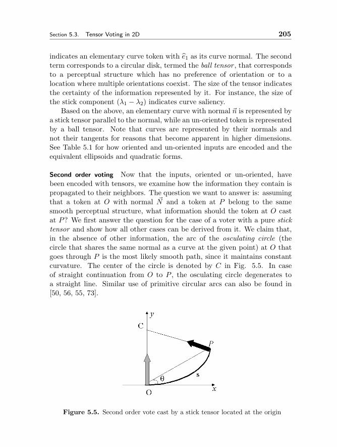
Section 5.3. Tensor Voting in 2D 205
indicates an elementary curve token with e1 as its curve normal. The secondterm corresponds to a circular disk, termed the ball tensor , that correspondsto a perceptual structure which has no preference of orientation or to alocation where multiple orientations coexist. The size of the tensor indicatesthe certainty of the information represented by it. For instance, the size ofthe stick component (λ1 − λ2) indicates curve saliency.
Based on the above, an elementary curve with normal n is represented bya stick tensor parallel to the normal, while an un-oriented token is representedby a ball tensor. Note that curves are represented by their normals andnot their tangents for reasons that become apparent in higher dimensions.See Table 5.1 for how oriented and un-oriented inputs are encoded and theequivalent ellipsoids and quadratic forms.
Second order voting Now that the inputs, oriented or un-oriented, havebeen encoded with tensors, we examine how the information they contain ispropagated to their neighbors. The question we want to answer is: assumingthat a token at O with normal N and a token at P belong to the samesmooth perceptual structure, what information should the token at O castat P? We first answer the question for the case of a voter with a pure sticktensor and show how all other cases can be derived from it. We claim that,in the absence of other information, the arc of the osculating circle (thecircle that shares the same normal as a curve at the given point) at O thatgoes through P is the most likely smooth path, since it maintains constantcurvature. The center of the circle is denoted by C in Fig. 5.5. In caseof straight continuation from O to P , the osculating circle degenerates toa straight line. Similar use of primitive circular arcs can also be found in[50, 56, 55, 73].
Figure 5.5. Second order vote cast by a stick tensor located at the origin

206 The Tensor Voting Framework Chapter 5
As shown in Fig. 5.5, the second order vote is also a stick tensor andhas a normal lying along the radius of the osculating circle at P . Whatremains to be defined is the magnitude of the vote. According to the Gestaltprinciples it should be a function of proximity and smooth continuation.The influence from a token to another should attenuate with distance, tominimize interference from unrelated tokens, and curvature, to favor straightcontinuation over curved alternatives when both exist. Moreover, no votesare cast if the receiver is at an angle larger than 45o with respect to thetangent of the osculating circle at the voter. Similar restrictions on the fieldsappear also in [19, 73, 36]. The saliency decay function we have selected hasthe following form:
DF (s, κ, σ) = e−( s2+cκ2
σ2 ) (5.2)
where s is the arc length OP , κ is the curvature, c controls the degree of decaywith curvature, and σ is the scale of voting, which determines the effectiveneighborhood size. The parameter c is a function of the scale and is optimizedto make the extension of two orthogonal line segments to form a right angleequally likely to the completion of the contour with a rounded corner [15]. Itsvalue is given by: c = −16log(0.1)×(σ−1)
π2 . Scale essentially controls the rangewithin which tokens can influence other tokens. The saliency decay functionhas infinite extend, but for practical reasons it is cropped at a distance wherethe votes cast become insignificant. For instance, the field can be definedup to the extend that vote strength becomes less than 1% of the voter’ssaliency. The scale of voting can also be viewed as a measure of smoothness.A large scale favors long range interactions and enforces a higher degree ofsmoothness, aiding noise removal at the same time, while a small scale makesthe voting process more local, thus preserving details. Note that σ is theonly free parameter in the system.
The 2-D second order stick voting field for a unit stick voter located atthe origin and aligned with the z-axis can be defined as follows as a functionof the distance l between the voter and receiver and the angle θ, which isthe angle between the tangent of the osculating circle at the voter and theline going through the voter and receiver (see Fig. 5.5).
SSO(d, θ) = DF (s, κ, σ)[ −sin(2θ)
cos(2θ)
][−sin(2θ) cos(2θ)]
s =θl
sin(θ), κ =
2sin(θ)l
(5.3)
The votes are also stick tensors. For stick tensors of arbitrary size the magni-tude of the vote is given by 5.2 multiplied by the the size of the stick λ1−λ2.
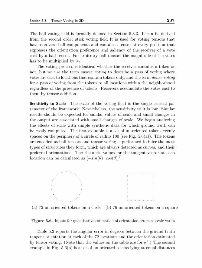
Section 5.3. Tensor Voting in 2D 207
The ball voting field is formally defined in Section 5.3.3. It can be derivedfrom the second order stick voting field It is used for voting tensors thathave non zero ball components and contain a tensor at every position thatexpresses the orientation preference and saliency of the receiver of a votecast by a ball tensor. For arbitrary ball tensors the magnitude of the voteshas to be multiplied by λ2.
The voting process is identical whether the receiver contains a token ornot, but we use the term sparse voting to describe a pass of voting wherevotes are cast to locations that contain tokens only, and the term dense votingfor a pass of voting from the tokens to all locations within the neighborhoodregardless of the presence of tokens. Receivers accumulate the votes cast tothem by tensor addition.
Sensitivity to Scale The scale of the voting field is the single critical pa-rameter of the framework. Nevertheless, the sensitivity to it is low. Similarresults should be expected for similar values of scale and small changes inthe output are associated with small changes of scale. We begin analyzingthe effects of scale with simple synthetic data for which ground truth canbe easily computed. The first example is a set of un-oriented tokens evenlyspaced on the periphery of a circle of radius 100 (see Fig. 5.6(a)). The tokensare encoded as ball tensors and tensor voting is performed to infer the mosttypes of structures they form, which are always detected as curves, and theirpreferred orientations. The theoretic values for the tangent vector at eachlocation can be calculated as [−sin(θ) cos(θ)]T .
(a) 72 un-oriented tokens on a circle (b) 76 un-oriented tokens on a square
Figure 5.6. Inputs for quantitative estimation of orientation errors as scale varies
Table 5.2 reports the angular error in degrees between the ground truthtangent orientation at each of the 72 locations and the orientation estimatedby tensor voting. (Note that the values on the table are for σ2.) The secondexample in Fig. 5.6(b) is a set of un-oriented tokens lying at equal distances
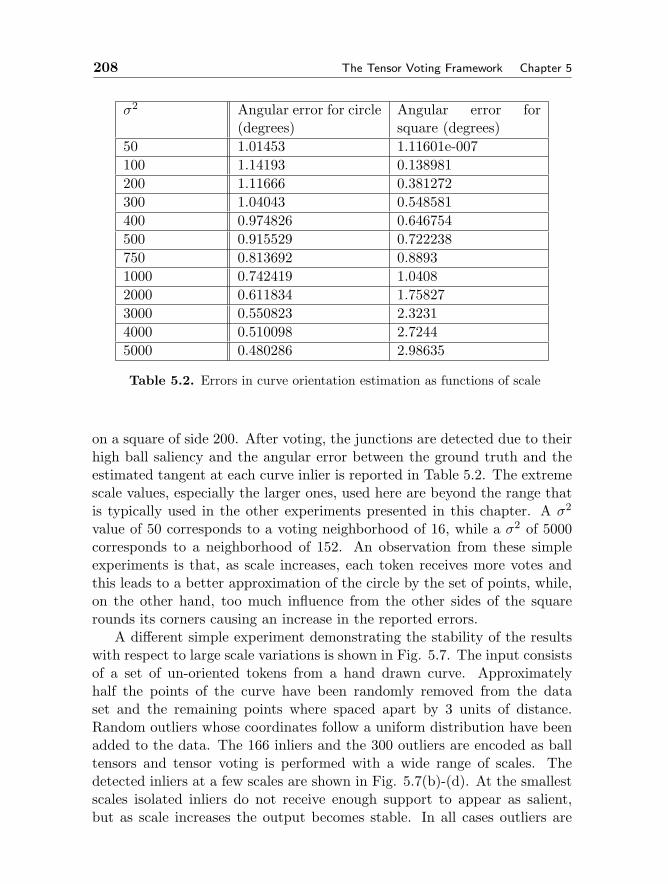
208 The Tensor Voting Framework Chapter 5
σ2 Angular error for circle(degrees)
Angular error forsquare (degrees)
50 1.01453 1.11601e-007100 1.14193 0.138981200 1.11666 0.381272300 1.04043 0.548581400 0.974826 0.646754500 0.915529 0.722238750 0.813692 0.88931000 0.742419 1.04082000 0.611834 1.758273000 0.550823 2.32314000 0.510098 2.72445000 0.480286 2.98635
Table 5.2. Errors in curve orientation estimation as functions of scale
on a square of side 200. After voting, the junctions are detected due to theirhigh ball saliency and the angular error between the ground truth and theestimated tangent at each curve inlier is reported in Table 5.2. The extremescale values, especially the larger ones, used here are beyond the range thatis typically used in the other experiments presented in this chapter. A σ2
value of 50 corresponds to a voting neighborhood of 16, while a σ2 of 5000corresponds to a neighborhood of 152. An observation from these simpleexperiments is that, as scale increases, each token receives more votes andthis leads to a better approximation of the circle by the set of points, while,on the other hand, too much influence from the other sides of the squarerounds its corners causing an increase in the reported errors.
A different simple experiment demonstrating the stability of the resultswith respect to large scale variations is shown in Fig. 5.7. The input consistsof a set of un-oriented tokens from a hand drawn curve. Approximatelyhalf the points of the curve have been randomly removed from the dataset and the remaining points where spaced apart by 3 units of distance.Random outliers whose coordinates follow a uniform distribution have beenadded to the data. The 166 inliers and the 300 outliers are encoded as balltensors and tensor voting is performed with a wide range of scales. Thedetected inliers at a few scales are shown in Fig. 5.7(b)-(d). At the smallestscales isolated inliers do not receive enough support to appear as salient,but as scale increases the output becomes stable. In all cases outliers are
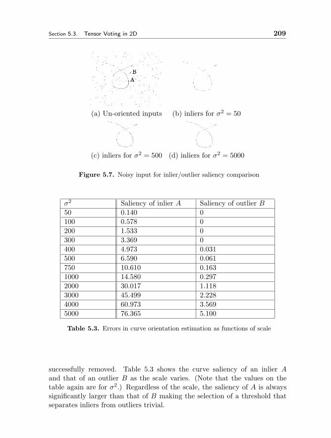
Section 5.3. Tensor Voting in 2D 209
(a) Un-oriented inputs (b) inliers for σ2 = 50
(c) inliers for σ2 = 500 (d) inliers for σ2 = 5000
Figure 5.7. Noisy input for inlier/outlier saliency comparison
σ2 Saliency of inlier A Saliency of outlier B50 0.140 0100 0.578 0200 1.533 0300 3.369 0400 4.973 0.031500 6.590 0.061750 10.610 0.1631000 14.580 0.2972000 30.017 1.1183000 45.499 2.2284000 60.973 3.5695000 76.365 5.100
Table 5.3. Errors in curve orientation estimation as functions of scale
successfully removed. Table 5.3 shows the curve saliency of an inlier Aand that of an outlier B as the scale varies. (Note that the values on thetable again are for σ2.) Regardless of the scale, the saliency of A is alwayssignificantly larger than that of B making the selection of a threshold thatseparates inliers from outliers trivial.
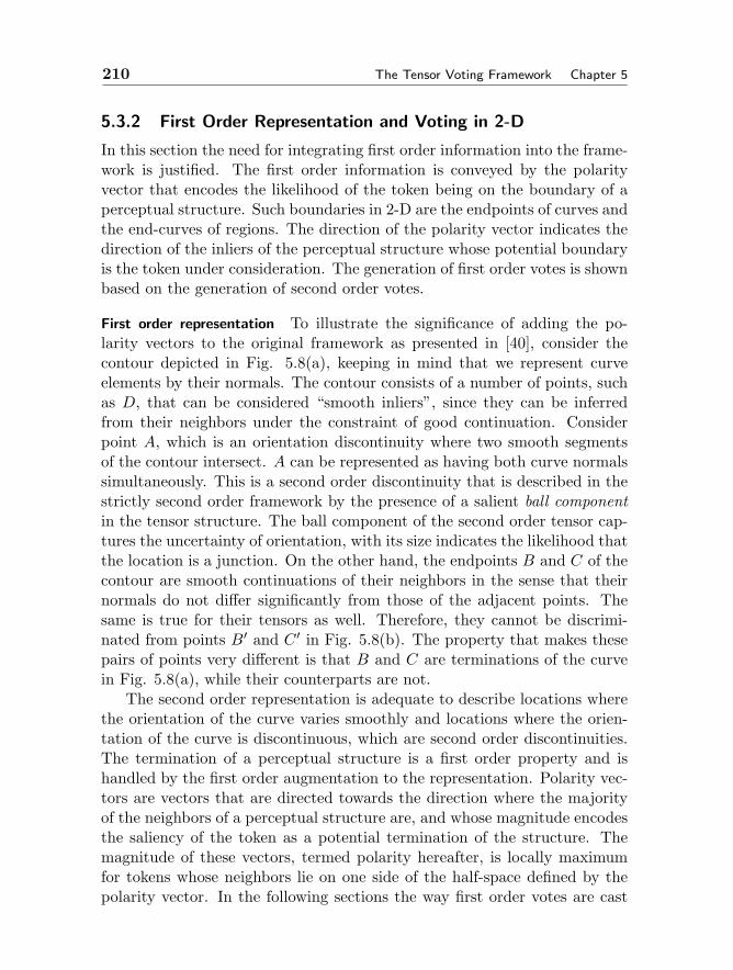
210 The Tensor Voting Framework Chapter 5
5.3.2 First Order Representation and Voting in 2-D
In this section the need for integrating first order information into the frame-work is justified. The first order information is conveyed by the polarityvector that encodes the likelihood of the token being on the boundary of aperceptual structure. Such boundaries in 2-D are the endpoints of curves andthe end-curves of regions. The direction of the polarity vector indicates thedirection of the inliers of the perceptual structure whose potential boundaryis the token under consideration. The generation of first order votes is shownbased on the generation of second order votes.
First order representation To illustrate the significance of adding the po-larity vectors to the original framework as presented in [40], consider thecontour depicted in Fig. 5.8(a), keeping in mind that we represent curveelements by their normals. The contour consists of a number of points, suchas D, that can be considered “smooth inliers”, since they can be inferredfrom their neighbors under the constraint of good continuation. Considerpoint A, which is an orientation discontinuity where two smooth segmentsof the contour intersect. A can be represented as having both curve normalssimultaneously. This is a second order discontinuity that is described in thestrictly second order framework by the presence of a salient ball componentin the tensor structure. The ball component of the second order tensor cap-tures the uncertainty of orientation, with its size indicates the likelihood thatthe location is a junction. On the other hand, the endpoints B and C of thecontour are smooth continuations of their neighbors in the sense that theirnormals do not differ significantly from those of the adjacent points. Thesame is true for their tensors as well. Therefore, they cannot be discrimi-nated from points B′ and C ′ in Fig. 5.8(b). The property that makes thesepairs of points very different is that B and C are terminations of the curvein Fig. 5.8(a), while their counterparts are not.
The second order representation is adequate to describe locations wherethe orientation of the curve varies smoothly and locations where the orien-tation of the curve is discontinuous, which are second order discontinuities.The termination of a perceptual structure is a first order property and ishandled by the first order augmentation to the representation. Polarity vec-tors are vectors that are directed towards the direction where the majorityof the neighbors of a perceptual structure are, and whose magnitude encodesthe saliency of the token as a potential termination of the structure. Themagnitude of these vectors, termed polarity hereafter, is locally maximumfor tokens whose neighbors lie on one side of the half-space defined by thepolarity vector. In the following sections the way first order votes are cast
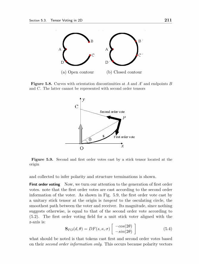
Section 5.3. Tensor Voting in 2D 211
(a) Open contour (b) Closed contour
Figure 5.8. Curves with orientation discontinuities at A and A′ and endpoints Band C. The latter cannot be represented with second order tensors
Figure 5.9. Second and first order votes cast by a stick tensor located at theorigin
and collected to infer polarity and structure terminations is shown.
First order voting Now, we turn our attention to the generation of first ordervotes. note that the first order votes are cast according to the second orderinformation of the voter. As shown in Fig. 5.9, the first order vote cast bya unitary stick tensor at the origin is tangent to the osculating circle, thesmoothest path between the voter and receiver. Its magnitude, since nothingsuggests otherwise, is equal to that of the second order vote according to(5.2). The first order voting field for a unit stick voter aligned with thez-axis is:
SFO(d, θ) = DF (s, κ, σ)[ −cos(2θ)−sin(2θ)
](5.4)
what should be noted is that tokens cast first and second order votes basedon their second order information only. This occurs because polarity vectors

212 The Tensor Voting Framework Chapter 5
(a) Input set of un-oriented tokens
(b) Saliency (c) Polarity
Figure 5.10. Accumulated saliency and polarity for a simple input
have to be initialized to zero since no assumption about structure termina-tions is available. Therefore, first order votes are computed based on thesecond order representation which can be initialized (in the form of balltensors) even with no information other than the presence of a token.
A simple illustration of how first and second order votes can be combinedto infer curves and their endpoints in 2-D appears in Fig. 5.10. The inputconsists of a set of colinear un-oriented tokens which are encoded as balltensors. The tokens cast votes to their neighbors and collect the votes castto them. The accumulated saliency can be seen in Fig. 5.10(b), where thedashed lines mark the limits of the input. The interior points of the curvereceive more support and are more salient than those close to the endpoints.Since second order voting is an excitatory process, locations beyond theendpoints are also compatible with the inferred line and receive consistentvotes from the input tokens. Detection of the endpoints based on the secondorder votes is virtually impossible since there is no systematic way of selectinga threshold that guarantees that the curve will not extend beyond the lastinput tokens. The strength of the second order aspect of the framework liesin the ability to extrapolate and fill in gaps caused by missing data. Theaccumulated polarity can be seen in Fig. 5.10(c). The endpoints appearclearly as maxima of polarity. The combination of saliency and polarityallows us to infer the curve and terminate it at the correct points. Seesection 5.3.4 for a complete analysis of structure inference in 2-D.
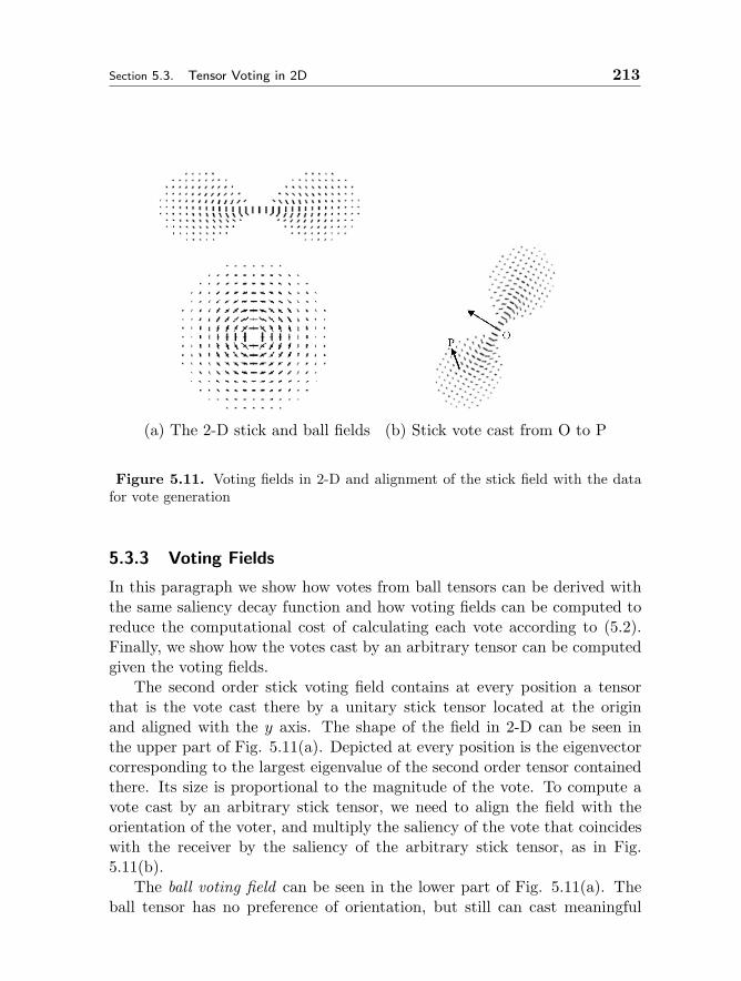
Section 5.3. Tensor Voting in 2D 213
(a) The 2-D stick and ball fields (b) Stick vote cast from O to P
Figure 5.11. Voting fields in 2-D and alignment of the stick field with the datafor vote generation
5.3.3 Voting Fields
In this paragraph we show how votes from ball tensors can be derived withthe same saliency decay function and how voting fields can be computed toreduce the computational cost of calculating each vote according to (5.2).Finally, we show how the votes cast by an arbitrary tensor can be computedgiven the voting fields.
The second order stick voting field contains at every position a tensorthat is the vote cast there by a unitary stick tensor located at the originand aligned with the y axis. The shape of the field in 2-D can be seen inthe upper part of Fig. 5.11(a). Depicted at every position is the eigenvectorcorresponding to the largest eigenvalue of the second order tensor containedthere. Its size is proportional to the magnitude of the vote. To compute avote cast by an arbitrary stick tensor, we need to align the field with theorientation of the voter, and multiply the saliency of the vote that coincideswith the receiver by the saliency of the arbitrary stick tensor, as in Fig.5.11(b).
The ball voting field can be seen in the lower part of Fig. 5.11(a). Theball tensor has no preference of orientation, but still can cast meaningful

214 The Tensor Voting Framework Chapter 5
Figure 5.12. Tensor addition in 2-D. Purely stick tensors result only from theaddition of parallel stick tensors and purely ball tensors from the addition of balltensors or orthogonal stick tensors
information to other locations. The presence of two proximate un-orientedtokens, the voter and the receiver, indicates a potential curve going throughthe two tokens. The ball voting fields allow us to infer preferred orientationsfrom un-oriented tokens, thus minimizing initialization requirements.
The derivation of the ball voting field B(P ) from the stick voting fieldcan be visualized as follows: the vote at P from a unitary ball tensor at theorigin O is the integration of the votes of stick tensors that span the space ofall possible orientations. In 2-D, this is equivalent to a rotating stick tensorthat spans the unit circle at O. The 2-D ball field can be derived from thestick field S(P ), according to:
B(P ) =∫ 2π
0R−1θ S(RθP )R−T
θ dθ (5.5)
where Rθ is the rotation matrix to align S with e1, the eigenvector corre-sponding to the maximum eigenvalue (the stick component), of the rotatingtensor at P .
In practice, the integration is approximated by tensor addition (see alsoFig. 5.12):
T =π∑i=0
π∑j=0
vivTi (5.6)
where V is the accumulated vote and vij are the stick votes, in vector form(which is equivalent since a stick tensor has only one non-zero eigenvalue andcan be expressed as the outer product of its only significant eigenvector),

Section 5.3. Tensor Voting in 2D 215
from O to P cast by the stick tensors i ∈ [0, 2π) that span the unit circle.Normalization has to be performed in order to make the energy emitted by aunitary ball equal to that of a unitary stick. As a result of the integration, thesecond order ball field does not contain purely stick or purely ball tensors, butarbitrary second order symmetric tensors. The field is radially symmetric,as expected, since the voter has no preferred orientation.
The 2-D first order stick voting field is a vector field, which at everyposition holds a vector that is equal in magnitude to the stick vote thatexists in the same position in the fundamental second order stick voting field,but is tangent to the smooth path between the voter and receiver insteadof normal to it. The first order ball voting field can be derived as in (5.5)by substituting the first order stick field for the second order stick field andperforming vector instead of tensor addition when integrating the votes ateach location.
All voting fields defined here, both first and second order, as well as allother fields in higher dimensions, are functions of the position of the receiverrelative to the voter, the tensor at the voter and a single parameter, the scaleof the saliency decay function. After these fields have been pre-computed atthe desired resolution, computing the votes cast by any second order tensoris reduced to a few look-up operations and linear interpolation. Voting takesplace in a finite neighborhood within which the magnitude of the votes castremains significant. For example, we can find the maximum distance smaxfrom the voter at which the vote cast will have 1% of the voter’s saliency, asfollows:
e−( s2maxσ2 ) = 0.01 (5.7)
The size of this neighborhood is obviously a function of the scale σ. Asdescribed in section 5.3.1, any tensor can be decomposed into the basis com-ponents (stick and ball in 2-D) according to its eigensystem. Then, the cor-responding fields can be aligned with each component. Votes are retrievedby simple look-up operations, and their magnitude is multiplied by the cor-responding saliency. The votes cast by the stick component are multipliedby λ1 − λ2 and those of the ball component by λ2.
5.3.4 Vote analysis
Votes are cast from token to token and accumulated by tensor addition in thecase of the second order votes, which are in general arbitrary second ordertensors, and by vector addition in the case of the first order votes, which arevectors.
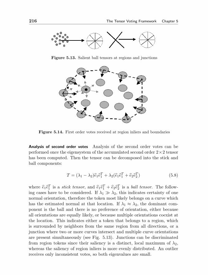
216 The Tensor Voting Framework Chapter 5
Figure 5.13. Salient ball tensors at regions and junctions
Figure 5.14. First order votes received at region inliers and boundaries
Analysis of second order votes Analysis of the second order votes can beperformed once the eigensystem of the accumulated second order 2×2 tensorhas been computed. Then the tensor can be decomposed into the stick andball components:
T = (λ1 − λ2)e1eT1 + λ2(e1eT1 + e2eT2 ) (5.8)
where e1eT1 is a stick tensor, and e1eT1 + e2e
T2 is a ball tensor. The follow-
ing cases have to be considered. If λ1 λ2, this indicates certainty of onenormal orientation, therefore the token most likely belongs on a curve whichhas the estimated normal at that location. If λ1 ≈ λ2, the dominant com-ponent is the ball and there is no preference of orientation, either becauseall orientations are equally likely, or because multiple orientations coexist atthe location. This indicates either a token that belongs to a region, whichis surrounded by neighbors from the same region from all directions, or ajunction where two or more curves intersect and multiple curve orientationsare present simultaneously (see Fig. 5.13). Junctions can be discriminatedfrom region tokens since their saliency is a distinct, local maximum of λ2,whereas the saliency of region inliers is more evenly distributed. An outlierreceives only inconsistent votes, so both eigenvalues are small.

Section 5.3. Tensor Voting in 2D 217
2-D Feature Saliency Secondorder tensororientation
Polarity Polarityvector
curve interior high λ1−λ2 normal: e1 low -curve endpoint high λ1−λ2 normal: e1 high parallel to
e2region interior high λ2 - low -region bound-ary
high λ2 - high normal toboundary
junction locally maxλ2
- low -
outlier low - low -
Table 5.4. Summary of first and second order tensor structure for each featuretype in 2-D
Analysis of first order votes Vote collection for the first order case is per-formed by vector addition. The accumulated result is a vector whose direc-tion points to a weighted center of mass from which votes are cast, and whosemagnitude encodes polarity. Since the first order votes are also weighted bythe saliency of the voters and attenuate with distance and curvature, theirvector sum points to the direction from which the most salient contributionswere received. A relatively low polarity indicates a token that is in the in-terior of a curve or region, therefore surrounded by neighbors whose votescancel out each other. On the other hand, a high polarity indicates a tokenthat is on or close to a boundary, thus receiving votes from only one sidewith respect to the boundary, at least locally. The correct boundaries can beextracted as maxima of polarity along the direction of the polarity vector.See the region of Fig. 5.14, where the votes received at interior points canceleach other out, while the votes at boundary points reinforce each other re-sulting in a large polarity vector there. Table 5.4 illustrates how tokens canbe characterized using the collected first and second order information.
Dense Structure Extraction In order to extract dense structures based onthe sparse set of tokens, an additional step is performed. Votes are collectedat every location to determine where salient structures exist. The processof collecting votes at all locations regardless of whether they contain aninput token or not is called dense voting . The tensors at every locationare decomposed and Saliency maps are built. In 2-D there are two types
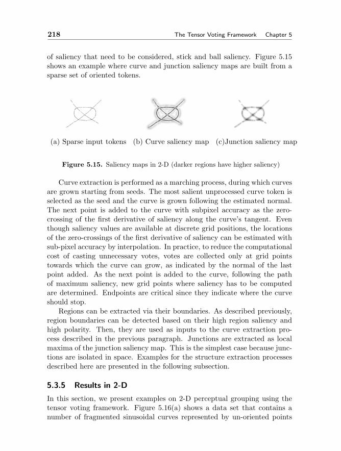
218 The Tensor Voting Framework Chapter 5
of saliency that need to be considered, stick and ball saliency. Figure 5.15shows an example where curve and junction saliency maps are built from asparse set of oriented tokens.
(a) Sparse input tokens (b) Curve saliency map (c)Junction saliency map
Figure 5.15. Saliency maps in 2-D (darker regions have higher saliency)
Curve extraction is performed as a marching process, during which curvesare grown starting from seeds. The most salient unprocessed curve token isselected as the seed and the curve is grown following the estimated normal.The next point is added to the curve with subpixel accuracy as the zero-crossing of the first derivative of saliency along the curve’s tangent. Eventhough saliency values are available at discrete grid positions, the locationsof the zero-crossings of the first derivative of saliency can be estimated withsub-pixel accuracy by interpolation. In practice, to reduce the computationalcost of casting unnecessary votes, votes are collected only at grid pointstowards which the curve can grow, as indicated by the normal of the lastpoint added. As the next point is added to the curve, following the pathof maximum saliency, new grid points where saliency has to be computedare determined. Endpoints are critical since they indicate where the curveshould stop.
Regions can be extracted via their boundaries. As described previously,region boundaries can be detected based on their high region saliency andhigh polarity. Then, they are used as inputs to the curve extraction pro-cess described in the previous paragraph. Junctions are extracted as localmaxima of the junction saliency map. This is the simplest case because junc-tions are isolated in space. Examples for the structure extraction processesdescribed here are presented in the following subsection.
5.3.5 Results in 2-D
In this section, we present examples on 2-D perceptual grouping using thetensor voting framework. Figure 5.16(a) shows a data set that contains anumber of fragmented sinusoidal curves represented by un-oriented points
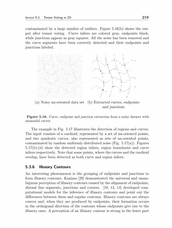
Section 5.3. Tensor Voting in 2D 219
contaminated by a large number of outliers. Figure 5.16(b) shows the out-put after tensor voting. Curve inliers are colored gray, endpoints black,while junctions appear as gray squares. All the noise has been removed andthe curve segments have been correctly detected and their endpoints andjunctions labeled.
(a) Noisy un-oriented data set (b) Extracted curves, endpointsand junctions
Figure 5.16. Curve, endpoint and junction extraction from a noisy dataset withsinusoidal curves
The example in Fig. 5.17 illustrates the detection of regions and curves.The input consists of a cardioid, represented by a set of un-oriented points,and two quadratic curves, also represented as sets of un-oriented points,contaminated by random uniformly distributed noise (Fig. 5.17(a)). Figures5.17(b)-(d) show the detected region inliers, region boundaries and curveinliers respectively. Note that some points, where the curves and the cardioidoverlap, have been detected as both curve and region inliers.
5.3.6 Illusory Contours
An interesting phenomenon is the grouping of endpoints and junctions toform illusory contours. Kanizsa [29] demonstrated the universal and unam-biguous perception of illusory contours caused by the alignment of endpoints,distant line segments, junctions and corners. [19, 13, 14] developed com-putational models for the inference of illusory contours and point out thedifferences between them and regular contours. Illusory contours are alwaysconvex and, when they are produced by endpoints, their formation occursin the orthogonal direction of the contours whose endpoints give rise to theillusory ones. A perception of an illusory contour is strong in the lower part
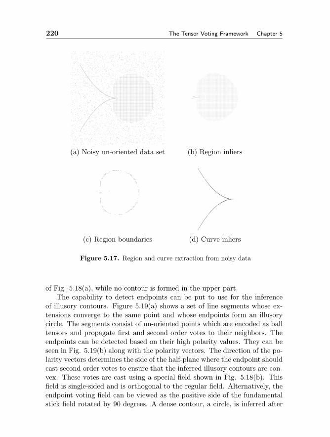
220 The Tensor Voting Framework Chapter 5
(a) Noisy un-oriented data set (b) Region inliers
(c) Region boundaries (d) Curve inliers
Figure 5.17. Region and curve extraction from noisy data
of Fig. 5.18(a), while no contour is formed in the upper part.The capability to detect endpoints can be put to use for the inference
of illusory contours. Figure 5.19(a) shows a set of line segments whose ex-tensions converge to the same point and whose endpoints form an illusorycircle. The segments consist of un-oriented points which are encoded as balltensors and propagate first and second order votes to their neighbors. Theendpoints can be detected based on their high polarity values. They can beseen in Fig. 5.19(b) along with the polarity vectors. The direction of the po-larity vectors determines the side of the half-plane where the endpoint shouldcast second order votes to ensure that the inferred illusory contours are con-vex. These votes are cast using a special field shown in Fig. 5.18(b). Thisfield is single-sided and is orthogonal to the regular field. Alternatively, theendpoint voting field can be viewed as the positive side of the fundamentalstick field rotated by 90 degrees. A dense contour, a circle, is inferred after
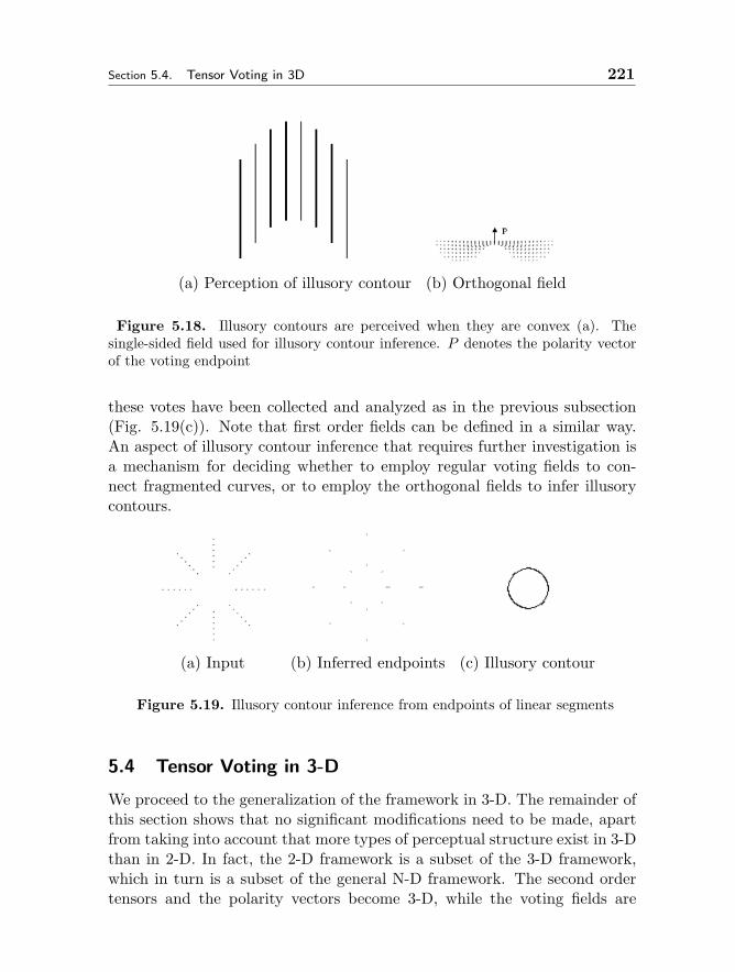
Section 5.4. Tensor Voting in 3D 221
(a) Perception of illusory contour (b) Orthogonal field
Figure 5.18. Illusory contours are perceived when they are convex (a). Thesingle-sided field used for illusory contour inference. P denotes the polarity vectorof the voting endpoint
these votes have been collected and analyzed as in the previous subsection(Fig. 5.19(c)). Note that first order fields can be defined in a similar way.An aspect of illusory contour inference that requires further investigation isa mechanism for deciding whether to employ regular voting fields to con-nect fragmented curves, or to employ the orthogonal fields to infer illusorycontours.
(a) Input (b) Inferred endpoints (c) Illusory contour
Figure 5.19. Illusory contour inference from endpoints of linear segments
5.4 Tensor Voting in 3-D
We proceed to the generalization of the framework in 3-D. The remainder ofthis section shows that no significant modifications need to be made, apartfrom taking into account that more types of perceptual structure exist in 3-Dthan in 2-D. In fact, the 2-D framework is a subset of the 3-D framework,which in turn is a subset of the general N-D framework. The second ordertensors and the polarity vectors become 3-D, while the voting fields are
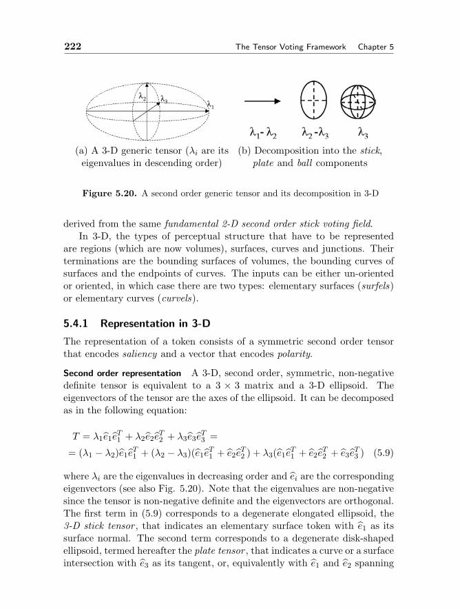
222 The Tensor Voting Framework Chapter 5
(a) A 3-D generic tensor (λi are its (b) Decomposition into the stick,eigenvalues in descending order) plate and ball components
Figure 5.20. A second order generic tensor and its decomposition in 3-D
derived from the same fundamental 2-D second order stick voting field.In 3-D, the types of perceptual structure that have to be represented
are regions (which are now volumes), surfaces, curves and junctions. Theirterminations are the bounding surfaces of volumes, the bounding curves ofsurfaces and the endpoints of curves. The inputs can be either un-orientedor oriented, in which case there are two types: elementary surfaces (surfels)or elementary curves (curvels).
5.4.1 Representation in 3-D
The representation of a token consists of a symmetric second order tensorthat encodes saliency and a vector that encodes polarity.
Second order representation A 3-D, second order, symmetric, non-negativedefinite tensor is equivalent to a 3 × 3 matrix and a 3-D ellipsoid. Theeigenvectors of the tensor are the axes of the ellipsoid. It can be decomposedas in the following equation:
T = λ1e1eT1 + λ2e2e
T2 + λ3e3e
T3 =
= (λ1 − λ2)e1eT1 + (λ2 − λ3)(e1eT1 + e2eT2 ) + λ3(e1eT1 + e2e
T2 + e3e
T3 ) (5.9)
where λi are the eigenvalues in decreasing order and ei are the correspondingeigenvectors (see also Fig. 5.20). Note that the eigenvalues are non-negativesince the tensor is non-negative definite and the eigenvectors are orthogonal.The first term in (5.9) corresponds to a degenerate elongated ellipsoid, the3-D stick tensor , that indicates an elementary surface token with e1 as itssurface normal. The second term corresponds to a degenerate disk-shapedellipsoid, termed hereafter the plate tensor , that indicates a curve or a surfaceintersection with e3 as its tangent, or, equivalently with e1 and e2 spanning
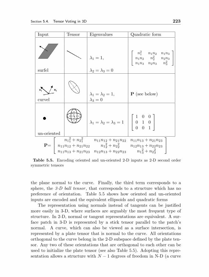
Section 5.4. Tensor Voting in 3D 223
Input Tensor Eigenvalues Quadratic form
λ1 = 1,
n21 n1n2 n1n3
n1n2 n22 n2n3
n1n3 n2n3 n23
surfel λ2 = λ3 = 0
λ1 = λ2 = 1, P (see below)curvel λ3 = 0
λ1 = λ2 = λ3 = 1
1 0 00 1 00 0 1
un-oriented
P=
n121 + n2
21 n11n12 + n21n22 n11n13 + n21n23
n11n12 + n21n22 n122 + n2
22 n12n13 + n22n23
n11n13 + n21n23 n12n13 + n22n23 n123 + n2
23
Table 5.5. Encoding oriented and un-oriented 2-D inputs as 2-D second order
symmetric tensors
the plane normal to the curve. Finally, the third term corresponds to asphere, the 3-D ball tensor , that corresponds to a structure which has nopreference of orientation. Table 5.5 shows how oriented and un-orientedinputs are encoded and the equivalent ellipsoids and quadratic forms
The representation using normals instead of tangents can be justifiedmore easily in 3-D, where surfaces are arguably the most frequent type ofstructure. In 2-D, normal or tangent representations are equivalent. A sur-face patch in 3-D is represented by a stick tensor parallel to the patch’snormal. A curve, which can also be viewed as a surface intersection, isrepresented by a plate tensor that is normal to the curve. All orientationsorthogonal to the curve belong in the 2-D subspace defined by the plate ten-sor. Any two of these orientations that are orthogonal to each other can beused to initialize the plate tensor (see also Table 5.5). Adopting this repre-sentation allows a structure with N − 1 degrees of freedom in N-D (a curve

224 The Tensor Voting Framework Chapter 5
in 2-D, a surface in 3-D) to be represented by a single vector, while a tangentrepresentation would require the definition of N−1 vectors that form a basisfor an (N-1)-D subspace. Assuming that this is the most frequent structurein the N-D space, our choice of representation makes the stick voting field,which corresponds to the elementary (N-1)-D variety, the basis from whichall other voting fields are derived.
First order representation The first order part of the representation is, again,a polarity vector whose size indicates the likelihood of the token being aboundary of a perceptual structure and which points towards the half-spacewhere the majority of the token’s neighbors are.
5.4.2 Voting in 3-D
Identically to the 2-D case, voting begins with a set of oriented and un-oriented tokens. Again, both second and first order votes are cast accordingto the second order tensor of the voter.
Second order voting In this section, we begin by showing how a voter witha purely stick tensor generates and casts votes, and then, derive the votingfields for the plate and ball cases. We chose to maintain voting as a functionof only the position of the receiver relative to the voter and of the voter’spreference of orientation. Therefore, we again address the problem of findingthe smoothest path between the voter and receiver by fitting arcs of theosculating circle, as described in Section 5.3.1.
Note that the voter, the receiver and the stick tensor at the voter definea plane. The voting procedure is restricted in this plane, thus making itidentical to the 2-D case. The second order vote, which is the surface normalat the receiver under the assumption that the voter and receiver belong tothe same smooth surface, is also a purely stick tensor in the plane (see alsoFig. 5.5). The magnitude of the vote is defined by the same saliency decayfunction, duplicated here for completeness.
DF (s, κ, σ) = e−( s2+cκ2
σ2 ) (5.10)
where s is the arc length OP , κ is the curvature, c is a constant whichcontrols the decay with high curvature, and σ is the scale of voting. Sparse,token to token voting is performed to estimate the preferred orientation oftokens, followed by dense voting during which saliency is computed at everygrid position.
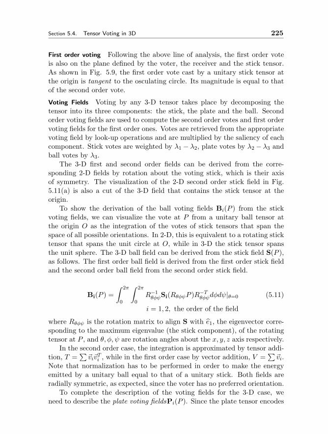
Section 5.4. Tensor Voting in 3D 225
First order voting Following the above line of analysis, the first order voteis also on the plane defined by the voter, the receiver and the stick tensor.As shown in Fig. 5.9, the first order vote cast by a unitary stick tensor atthe origin is tangent to the osculating circle. Its magnitude is equal to thatof the second order vote.
Voting Fields Voting by any 3-D tensor takes place by decomposing thetensor into its three components: the stick, the plate and the ball. Secondorder voting fields are used to compute the second order votes and first ordervoting fields for the first order ones. Votes are retrieved from the appropriatevoting field by look-up operations and are multiplied by the saliency of eachcomponent. Stick votes are weighted by λ1 − λ2, plate votes by λ2 − λ3 andball votes by λ3.
The 3-D first and second order fields can be derived from the corre-sponding 2-D fields by rotation about the voting stick, which is their axisof symmetry. The visualization of the 2-D second order stick field in Fig.5.11(a) is also a cut of the 3-D field that contains the stick tensor at theorigin.
To show the derivation of the ball voting fields Bi(P ) from the stickvoting fields, we can visualize the vote at P from a unitary ball tensor atthe origin O as the integration of the votes of stick tensors that span thespace of all possible orientations. In 2-D, this is equivalent to a rotating sticktensor that spans the unit circle at O, while in 3-D the stick tensor spansthe unit sphere. The 3-D ball field can be derived from the stick field S(P ),as follows. The first order ball field is derived from the first order stick fieldand the second order ball field from the second order stick field.
Bi(P ) =∫ 2π
0
∫ 2π
0R−1θφψSi(RθφψP )R−T
θφψdφdψ|θ=0 (5.11)
i = 1, 2, the order of the field
where Rθφψ is the rotation matrix to align S with e1, the eigenvector corre-sponding to the maximum eigenvalue (the stick component), of the rotatingtensor at P , and θ, φ, ψ are rotation angles about the x, y, z axis respectively.
In the second order case, the integration is approximated by tensor addi-tion, T =
∑viv
Ti , while in the first order case by vector addition, V =
∑vi.
Note that normalization has to be performed in order to make the energyemitted by a unitary ball equal to that of a unitary stick. Both fields areradially symmetric, as expected, since the voter has no preferred orientation.
To complete the description of the voting fields for the 3-D case, weneed to describe the plate voting fieldsPi(P ). Since the plate tensor encodes
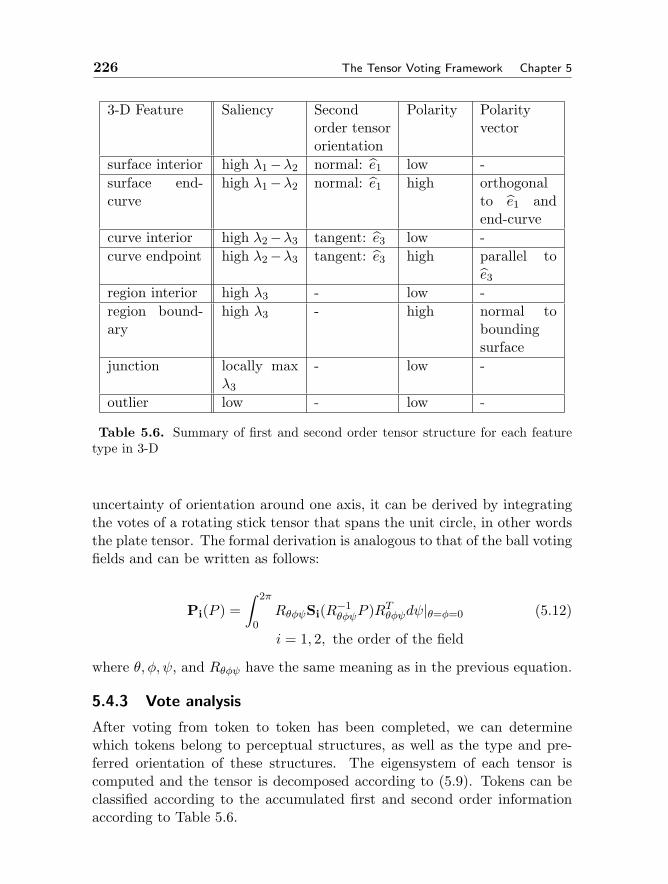
226 The Tensor Voting Framework Chapter 5
3-D Feature Saliency Secondorder tensororientation
Polarity Polarityvector
surface interior high λ1−λ2 normal: e1 low -surface end-curve
high λ1−λ2 normal: e1 high orthogonalto e1 andend-curve
curve interior high λ2−λ3 tangent: e3 low -curve endpoint high λ2−λ3 tangent: e3 high parallel to
e3region interior high λ3 - low -region bound-ary
high λ3 - high normal toboundingsurface
junction locally maxλ3
- low -
outlier low - low -
Table 5.6. Summary of first and second order tensor structure for each featuretype in 3-D
uncertainty of orientation around one axis, it can be derived by integratingthe votes of a rotating stick tensor that spans the unit circle, in other wordsthe plate tensor. The formal derivation is analogous to that of the ball votingfields and can be written as follows:
Pi(P ) =∫ 2π
0RθφψSi(R−1
θφψP )RTθφψdψ|θ=φ=0 (5.12)
i = 1, 2, the order of the field
where θ, φ, ψ, and Rθφψ have the same meaning as in the previous equation.
5.4.3 Vote analysis
After voting from token to token has been completed, we can determinewhich tokens belong to perceptual structures, as well as the type and pre-ferred orientation of these structures. The eigensystem of each tensor iscomputed and the tensor is decomposed according to (5.9). Tokens can beclassified according to the accumulated first and second order informationaccording to Table 5.6.
Section 5.4. Tensor Voting in 3D 227
Dense Structure Extraction Now that the most likely type of feature at eachtoken has been estimated, we want to compute the dense structures (curves,surfaces and volumes in 3-D) that can be inferred from the tokens. Con-tinuous structures are again extracted through the computation of saliencymaps. Three saliency maps need to be built: one that contains λ1 − λ2 atevery location, one for λ2 − λ3 and one for λ3. This can be achieved bycasting votes to all locations, whether they contain a token or not (densevoting).
Figure 5.21. Dense surface extraction in 3-D. (a) Elementary surface patch withnormal n. (b) 3-D surface saliency along normal direction (c) First derivative ofsurface saliency along normal direction
Figure 5.22. Dense curve extraction in 3-D. (a) 3-D curve with tangent t andthe normal plane. (b) Curve saliency iso-contours on the normal plane (c) Firstderivatives of surface saliency on the normal plane
Surfaces and curves are extracted using a modified marching algorithm[62] (based on the marching cubes algorithm [37]). They correspond to zerocrossings of the first derivative of the corresponding saliency. Junctions are
228 The Tensor Voting Framework Chapter 5
isolated and can be detected as distinct local maxima of λ3. Volume inliersare characterized by high λ3 values. Their bounding surfaces also have highλ3 values and high polarity, with polarity vectors being normal to the surfaceand pointing towards the interior of the region. Volumes are extracted asregions of high λ3, terminated at their boundaries which have high λ3 andhigh polarity. Junctions are isolated, distinct maxima of λ3.
In order to reduce the computational cost, the accumulation of votes atlocations with no prior information and structure extraction are integratedand performed as a marching process. Beginning from seeds, locations withhighest saliency, we perform a dense vote only towards the directions dictatedby the orientation of the features. Surfaces are extracted with sub-voxelaccuracy, as the zero-crossings of the first derivative of surface saliency (Fig.5.21). As in the 2-D case, discrete saliency values are computed at grid pointsand the continuous function is approximated via interpolation. Locationswith high surface saliency are selected as seeds for surface extraction, whilelocations with high curve saliency are selected as seeds for curve extraction.The marching direction in the former case is perpendicular to the surfacenormal, while, in the latter case, the marching direction is along the curve’stangent (Fig. 5.22).
5.4.4 Results in 3-D
In this section we present results on synthetic 3-D datasets corrupted byrandom noise. The first example is on a dataset that contains a surfacein the from of a spiral inside a cloud of noisy points (Fig. 5.23). Both thesurface and the noise are encoded as un-oriented points. The spiral consists of19,000 points, while the outliers are 30,000. Figure 5.23(b) shows the surfaceboundaries detected after voting. As the spiral is tightened to resemble acylinder (Fig. 5.23(c)), the surfaces merge and the inferred boundaries arethose of a cylinder (Fig. 5.23(d)).
The example in Fig. 5.24 illustrates the detection of regions and curves.The input consists of a “peanut” and a plane, encoded as un-oriented pointscontaminated by random uniformly distributed noise (Fig. 5.24(a)). The”peanut” is empty inside, except for the presence of noise, which has an equalprobability of being anywhere in space. Figure 5.24(c) shows the detectedsurface inliers, after tokens with low saliency have been removed. Figure5.24(c) shows the curve inliers, that is the tokens that lie at the intersectionof the two surfaces. Finally, Fig. 5.24(d) shows the extracted dense surfaces.
Figure 5.25(a) shows two solid generalized cylinders with different parabolicsweep functions. The cylinder are generated by a uniform random distribu-
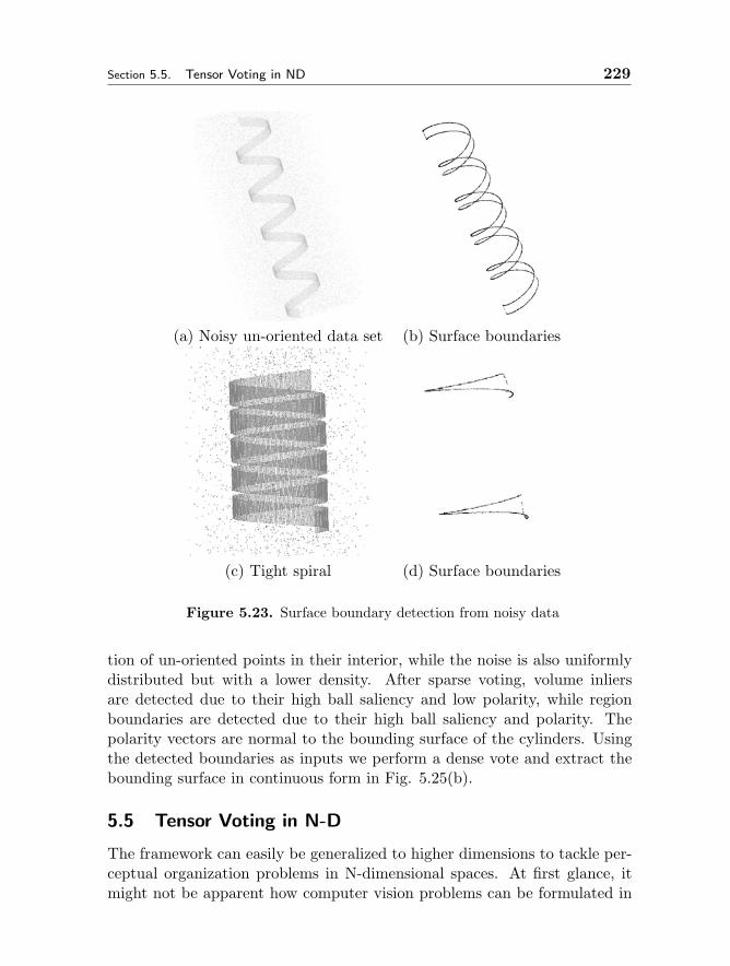
Section 5.5. Tensor Voting in ND 229
(a) Noisy un-oriented data set (b) Surface boundaries
(c) Tight spiral (d) Surface boundaries
Figure 5.23. Surface boundary detection from noisy data
tion of un-oriented points in their interior, while the noise is also uniformlydistributed but with a lower density. After sparse voting, volume inliersare detected due to their high ball saliency and low polarity, while regionboundaries are detected due to their high ball saliency and polarity. Thepolarity vectors are normal to the bounding surface of the cylinders. Usingthe detected boundaries as inputs we perform a dense vote and extract thebounding surface in continuous form in Fig. 5.25(b).
5.5 Tensor Voting in N-D
The framework can easily be generalized to higher dimensions to tackle per-ceptual organization problems in N-dimensional spaces. At first glance, itmight not be apparent how computer vision problems can be formulated in
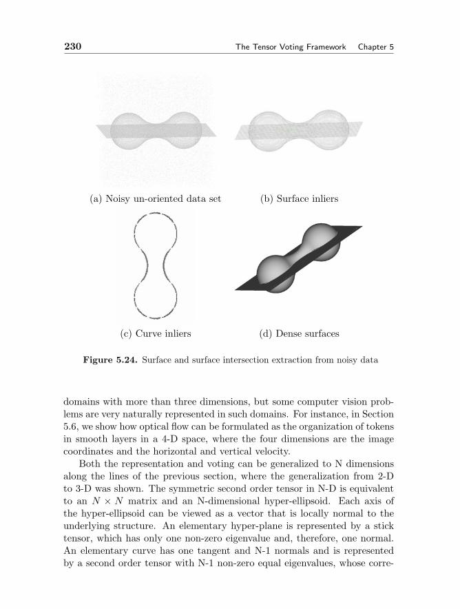
230 The Tensor Voting Framework Chapter 5
(a) Noisy un-oriented data set (b) Surface inliers
(c) Curve inliers (d) Dense surfaces
Figure 5.24. Surface and surface intersection extraction from noisy data
domains with more than three dimensions, but some computer vision prob-lems are very naturally represented in such domains. For instance, in Section5.6, we show how optical flow can be formulated as the organization of tokensin smooth layers in a 4-D space, where the four dimensions are the imagecoordinates and the horizontal and vertical velocity.
Both the representation and voting can be generalized to N dimensionsalong the lines of the previous section, where the generalization from 2-Dto 3-D was shown. The symmetric second order tensor in N-D is equivalentto an N × N matrix and an N-dimensional hyper-ellipsoid. Each axis ofthe hyper-ellipsoid can be viewed as a vector that is locally normal to theunderlying structure. An elementary hyper-plane is represented by a sticktensor, which has only one non-zero eigenvalue and, therefore, one normal.An elementary curve has one tangent and N-1 normals and is representedby a second order tensor with N-1 non-zero equal eigenvalues, whose corre-
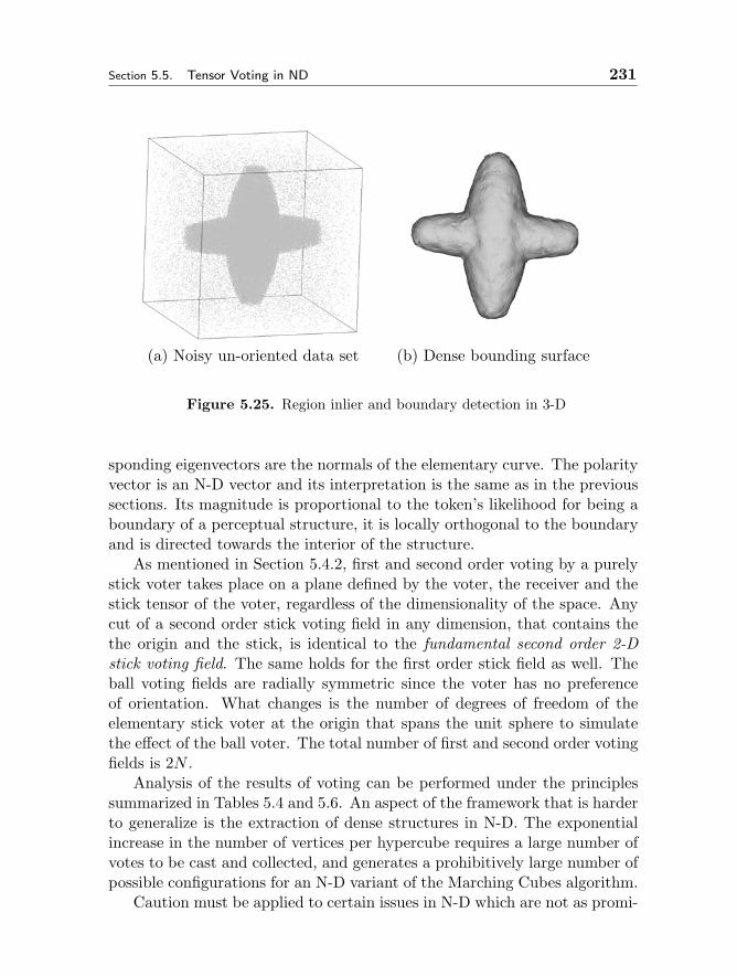
Section 5.5. Tensor Voting in ND 231
(a) Noisy un-oriented data set (b) Dense bounding surface
Figure 5.25. Region inlier and boundary detection in 3-D
sponding eigenvectors are the normals of the elementary curve. The polarityvector is an N-D vector and its interpretation is the same as in the previoussections. Its magnitude is proportional to the token’s likelihood for being aboundary of a perceptual structure, it is locally orthogonal to the boundaryand is directed towards the interior of the structure.
As mentioned in Section 5.4.2, first and second order voting by a purelystick voter takes place on a plane defined by the voter, the receiver and thestick tensor of the voter, regardless of the dimensionality of the space. Anycut of a second order stick voting field in any dimension, that contains thethe origin and the stick, is identical to the fundamental second order 2-Dstick voting field. The same holds for the first order stick field as well. Theball voting fields are radially symmetric since the voter has no preferenceof orientation. What changes is the number of degrees of freedom of theelementary stick voter at the origin that spans the unit sphere to simulatethe effect of the ball voter. The total number of first and second order votingfields is 2N .
Analysis of the results of voting can be performed under the principlessummarized in Tables 5.4 and 5.6. An aspect of the framework that is harderto generalize is the extraction of dense structures in N-D. The exponentialincrease in the number of vertices per hypercube requires a large number ofvotes to be cast and collected, and generates a prohibitively large number ofpossible configurations for an N-D variant of the Marching Cubes algorithm.
Caution must be applied to certain issues in N-D which are not as promi-
232 The Tensor Voting Framework Chapter 5
nent in two or three dimensions. Since voting is a function of distance andcurvature, these measures have to be meaningful. The space has to be Eu-clidean, or, at least, the axes have to be scaled in a way that distances aremeaningful, thus making the effect of more relevant neighbors larger thanthe effect of irrelevant ones. The data are stored in an Approximate Near-est Neighbor (ANN) k-d tree [1], and thus the computational complexityof searching for a token’s neighbors is linear with the dimensionality of thespace. Finally, depending on the number of input tokens and the dimen-sionality of the space, the pre-computation of the voting fields may becomeimpractical. If the data is relatively sparse in a high dimensional space, itis more efficient to compute the required votes when they are cast, insteadof generating complete voting fields and using them as look-up tables. Forsparse data in high dimensions, repetition of votes is less probable and manyof the pre-computed votes may never be used.
5.5.1 Computational Complexity
In this section, the computational complexity of tensor voting is analyzed.We show that it is a function of the number of tokens and, in the case ofdense structure extraction, the size of the extracted structures.
The initialization step consists of sorting the tokens according to theirspacial coordinates and storing them in a data structure from which they canbe retrieved efficiently. We use the ANN k-d tree as the data structure thatholds the tokens. Its construction is of O(dn logn) complexity, where d isthe dimension of the space and n the number of tokens. This data structuremeets the requirements of tensor voting operations, since it is optimal whenthe locations of the data remain constant and multiple queries that seek thedata points within a certain distance from a given location are generated.During voting, the tokens that are within the neighborhood of the voter, asdefined by the scale (see equation 5.7 in Section 5.3.4), can be retrieved withO(logn) operations.
The number of votes cast by a voter is not fixed and depends on thedistribution of data in space and the scale of voting. For most practicalpurposes, however, we can assume that each voter casts votes on a fractionof the dataset and that votes being cast to all tokens is the undesirable con-sequence of an extremely large scale. On average, the number of votes castby each voter can be approximated as the product of data density times thesize of the voting field. For each voter and receiver pair, the N componentsof the voter cast first and second order votes which are computed by look-upoperations from the voting fields and linear interpolation. The complexity

Section 5.6. Application to Computer Vision Problems 233
of voting, after the receivers have been localized, is linear in the number oftokens and the dimension of the space.
The complexity of dense structure extraction, which is implemented in 2-and 3-D only, is a function of grid resolution. since it defines the number ofcurvels or surfels extracted. The surface or curve saliency of a fixed number ofgrid points has to be computed for each surfel or curvel. For instance, surfacesaliency values at the eight vertices of a grid cube have to be computed for asurfel to be extracted at sub-voxel accuracy inside the cube. The search fortokens within the voting neighborhood of each vertex, from which votes arecollected, is O(m), where m is the number of vertices. The marching cubesalgorithm [37] is also linear, since it essentially consists of look-up operations.The number of voxels that are visited, but where no surface is extracted, istypically small (zero for a closed surface). Therefore the complexity of densesurface extraction in 3-D is O(mlogn), where n is the number of tokens andm the number of surfels. The same holds for curve extraction.
5.6 Application of the Tensor Voting Framework to Com-puter Vision Problems
Thus far, we have demonstrated the capability of the tensor voting frameworkto group oriented and un-oriented tokens into perceptual structures, as wellas to remove noise. In practice, however, we rarely have input data in theform we used for the examples of Sections 5.3.5 and 5.4.4, except maybe forrange or medical data. In this section, the focus will be on vision problems,where the input is images, while the desired output varies from applicationto application, but is some form of scene interpretation in terms of objectsand layers.
The missing piece that bridges the gap from the images to the type ofinput required by the framework is a set of application-specific processesthat can generate the tokens from the images. These relatively simple toolsenable us to address a variety of computer vision problems within the tensorvoting framework, alleviating the need to design software packages dedicatedto specific problems. The premise is that solutions to these problems mustcomprise coherent structures that are salient due to the non-accidental align-ment of simpler tokens. The fact that these solutions might come in differentforms, such as image segments, 3-D curves or motion layers, does not posean additional difficulty to the framework, since they are all characterized bynon-accidentalness and good continuation. As mentioned in Section 5.1.1,problem specific constraints can easily be incorporated as modules into theframework. For instance, uniqueness along the lines of sight can be enforced
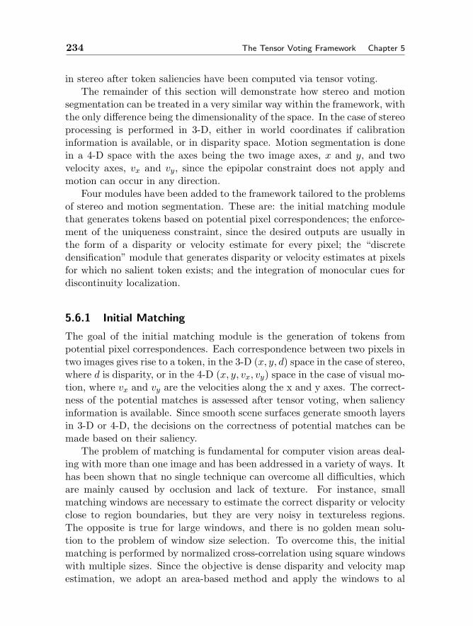
234 The Tensor Voting Framework Chapter 5
in stereo after token saliencies have been computed via tensor voting.The remainder of this section will demonstrate how stereo and motion
segmentation can be treated in a very similar way within the framework, withthe only difference being the dimensionality of the space. In the case of stereoprocessing is performed in 3-D, either in world coordinates if calibrationinformation is available, or in disparity space. Motion segmentation is donein a 4-D space with the axes being the two image axes, x and y, and twovelocity axes, vx and vy, since the epipolar constraint does not apply andmotion can occur in any direction.
Four modules have been added to the framework tailored to the problemsof stereo and motion segmentation. These are: the initial matching modulethat generates tokens based on potential pixel correspondences; the enforce-ment of the uniqueness constraint, since the desired outputs are usually inthe form of a disparity or velocity estimate for every pixel; the “discretedensification” module that generates disparity or velocity estimates at pixelsfor which no salient token exists; and the integration of monocular cues fordiscontinuity localization.
5.6.1 Initial Matching
The goal of the initial matching module is the generation of tokens frompotential pixel correspondences. Each correspondence between two pixels intwo images gives rise to a token, in the 3-D (x, y, d) space in the case of stereo,where d is disparity, or in the 4-D (x, y, vx, vy) space in the case of visual mo-tion, where vx and vy are the velocities along the x and y axes. The correct-ness of the potential matches is assessed after tensor voting, when saliencyinformation is available. Since smooth scene surfaces generate smooth layersin 3-D or 4-D, the decisions on the correctness of potential matches can bemade based on their saliency.
The problem of matching is fundamental for computer vision areas deal-ing with more than one image and has been addressed in a variety of ways. Ithas been shown that no single technique can overcome all difficulties, whichare mainly caused by occlusion and lack of texture. For instance, smallmatching windows are necessary to estimate the correct disparity or velocityclose to region boundaries, but they are very noisy in textureless regions.The opposite is true for large windows, and there is no golden mean solu-tion to the problem of window size selection. To overcome this, the initialmatching is performed by normalized cross-correlation using square windowswith multiple sizes. Since the objective is dense disparity and velocity mapestimation, we adopt an area-based method and apply the windows to al
Section 5.6. Application to Computer Vision Problems 235
pixels. Peaks in the cross-correlation function of each window size are re-tained as potential correspondences. The emphasis is towards detecting asmany correct correspondences as possible, at the expense of a possibly largenumber of wrong ones, which can be rejected after tensor voting.
(a) Left image (b) Initial matches
Figure 5.26. One of the two input frames and the initial matches for the Venusdataset. The view of the initial matches is rotated in the 3-D (x, y, d) space
The candidate matches are encoded in the appropriate space as ball ten-sors, having no bias for a specific orientation, or as stick tensors, biasedtowards locally fronto-parallel surfaces. Since the correct orientation canbe estimated with un-oriented inputs, and, moreover, a totally wrong ini-tialization with stick tensors would have adverse effects on the solution, weinitialize the tokens with ball tensors. Even though the matching score canbe used as the initial saliency of the tensor, we prefer to ignore it and initial-ize all tensors with unit saliency. This allows the seamless combination ofmultiple matchers, including non-correlation based ones. The output of theinitial matching module is a cloud of points in which the inliers form salientsurfaces. Figure 5.26 shows one of the input images of the stereo pair andthe initial matches for the “Venus” dataset from [57]).
5.6.2 Uniqueness
Another constraint that is specific to the problems of stereo and motion isthat of uniqueness. The required output is usually a disparity or velocityestimate for every pixel in the reference image. Therefore, after sparse vot-ing, the most salient token for each pixel position is retained and the othercandidates are rejected. In the case of stereo, we are interested in surfacesaliency since even thin objects can be viewed as thin surface patches thatreflect light to the cameras. Therefore, the criterion for determining the
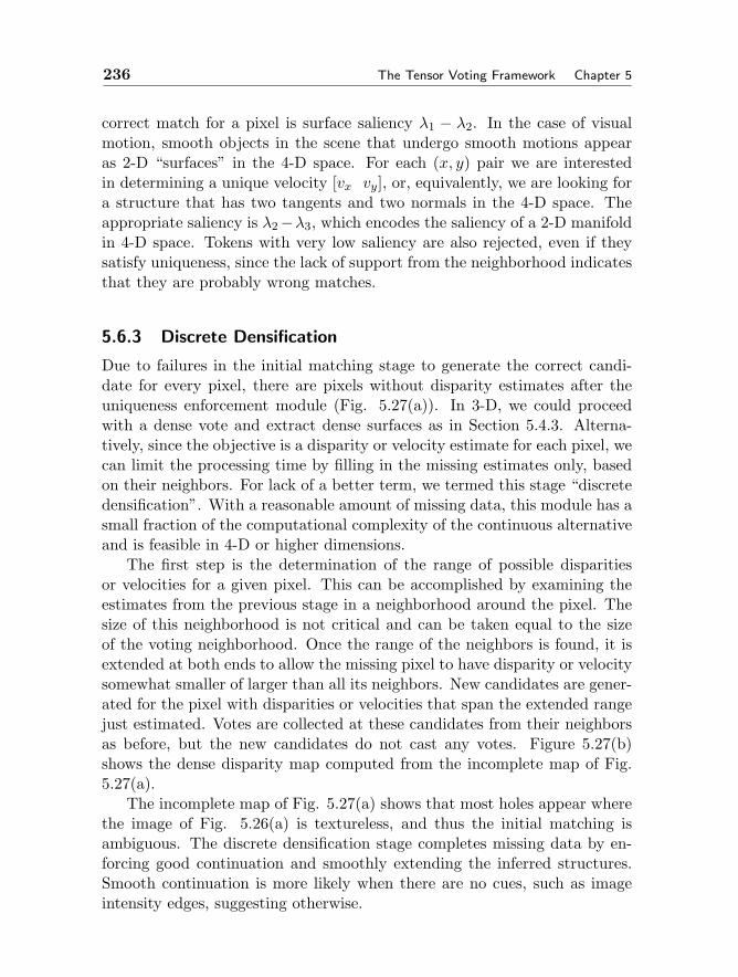
236 The Tensor Voting Framework Chapter 5
correct match for a pixel is surface saliency λ1 − λ2. In the case of visualmotion, smooth objects in the scene that undergo smooth motions appearas 2-D “surfaces” in the 4-D space. For each (x, y) pair we are interestedin determining a unique velocity [vx vy], or, equivalently, we are looking fora structure that has two tangents and two normals in the 4-D space. Theappropriate saliency is λ2−λ3, which encodes the saliency of a 2-D manifoldin 4-D space. Tokens with very low saliency are also rejected, even if theysatisfy uniqueness, since the lack of support from the neighborhood indicatesthat they are probably wrong matches.
5.6.3 Discrete Densification
Due to failures in the initial matching stage to generate the correct candi-date for every pixel, there are pixels without disparity estimates after theuniqueness enforcement module (Fig. 5.27(a)). In 3-D, we could proceedwith a dense vote and extract dense surfaces as in Section 5.4.3. Alterna-tively, since the objective is a disparity or velocity estimate for each pixel, wecan limit the processing time by filling in the missing estimates only, basedon their neighbors. For lack of a better term, we termed this stage “discretedensification”. With a reasonable amount of missing data, this module has asmall fraction of the computational complexity of the continuous alternativeand is feasible in 4-D or higher dimensions.
The first step is the determination of the range of possible disparitiesor velocities for a given pixel. This can be accomplished by examining theestimates from the previous stage in a neighborhood around the pixel. Thesize of this neighborhood is not critical and can be taken equal to the sizeof the voting neighborhood. Once the range of the neighbors is found, it isextended at both ends to allow the missing pixel to have disparity or velocitysomewhat smaller of larger than all its neighbors. New candidates are gener-ated for the pixel with disparities or velocities that span the extended rangejust estimated. Votes are collected at these candidates from their neighborsas before, but the new candidates do not cast any votes. Figure 5.27(b)shows the dense disparity map computed from the incomplete map of Fig.5.27(a).
The incomplete map of Fig. 5.27(a) shows that most holes appear wherethe image of Fig. 5.26(a) is textureless, and thus the initial matching isambiguous. The discrete densification stage completes missing data by en-forcing good continuation and smoothly extending the inferred structures.Smooth continuation is more likely when there are no cues, such as imageintensity edges, suggesting otherwise.
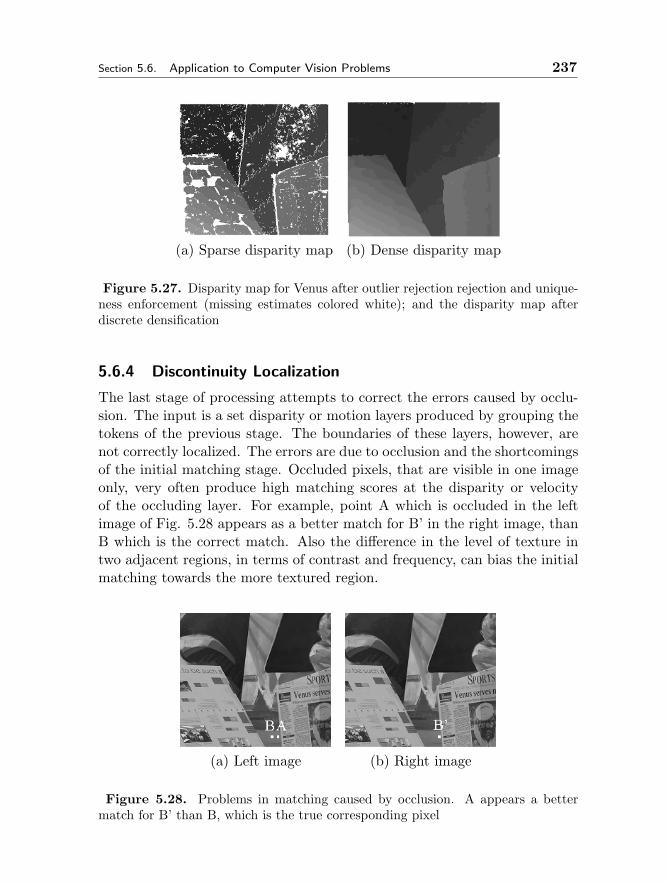
Section 5.6. Application to Computer Vision Problems 237
(a) Sparse disparity map (b) Dense disparity map
Figure 5.27. Disparity map for Venus after outlier rejection rejection and unique-ness enforcement (missing estimates colored white); and the disparity map afterdiscrete densification
5.6.4 Discontinuity Localization
The last stage of processing attempts to correct the errors caused by occlu-sion. The input is a set disparity or motion layers produced by grouping thetokens of the previous stage. The boundaries of these layers, however, arenot correctly localized. The errors are due to occlusion and the shortcomingsof the initial matching stage. Occluded pixels, that are visible in one imageonly, very often produce high matching scores at the disparity or velocityof the occluding layer. For example, point A which is occluded in the leftimage of Fig. 5.28 appears as a better match for B’ in the right image, thanB which is the correct match. Also the difference in the level of texture intwo adjacent regions, in terms of contrast and frequency, can bias the initialmatching towards the more textured region.
(a) Left image (b) Right image
Figure 5.28. Problems in matching caused by occlusion. A appears a bettermatch for B’ than B, which is the true corresponding pixel

238 The Tensor Voting Framework Chapter 5
Since it is hard to detect the problematic regions during initial match-ing, we propose a post-processing step to correct this type of errors whichwas first published in [48] for the case of motion. Since binocular cues areunreliable next to layer boundaries due to occlusion, we have to resort tomonocular information. A reasonable assumption is that the intensity dis-tributions of two surfaces that are distant in the scene, but appear adjacentfrom a particular viewpoint, should be quite different. Therefore, the pres-ence of a discontinuity in the scene should also be accompanied by an edgein the image. Instead of detecting edges in the entire image and having todiscriminate between true discontinuities and texture edges, we propose tofocus on “uncertainty zones” around the boundaries inferred at the previ-ous stage. The width of the uncertainty zones depends on the half-size ofthe matching window, since this is the maximum surface over-extension, aswell as the width of the occluded region, which can be estimated from thedifference in disparity or velocity at the boundary. In practice we mark asuncertain the entire occluded area extended by half the size of the maximummatching window on either side.
Once the uncertainty zones have been labelled as such, we look for edgesin them rather than the entire image. This is done by tensor voting in 2-Dsince some of the edges we are looking for may be fragmented or consist ofaligned edgels of low contrast. The initialization is performed by runninga simple gradient operator and initializing tokens at each pixel position asstick tensors whose orientation is given by the gradient and whose saliencyis given by:
Sal(x, y) = G(x, y)× e−(x−xo)2
σ2e (5.13)
where G(x, y) is the magnitude of the gradient at (x, y), xo is the position ofthe original layer boundary and σe is a function of the width of the uncer-tainty zone. The exponential term serves as a prior that biases the extractededges towards the original layer boundaries, and more importantly towardsthe direction of the original boundaries. That is, a vertical boundary is moresalient in a region where an almost vertical boundary was originally detected.This makes the edge detection scheme more robust to texture edges of dif-ferent orientations. Voting is performed in 2-D with these tokens as inputsand edges are extracted starting from seeds, tokens with maximum curvesaliency, and growing. Voting enables the completion of fragmented edgeswhile the interference by spurious strong responses of the gradient is notcatastrophic. Results for the example of Fig. 5.28 can be seen in Fig. 5.29.
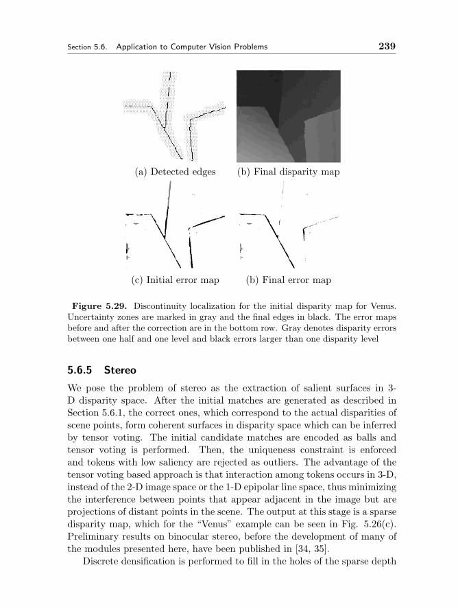
Section 5.6. Application to Computer Vision Problems 239
(a) Detected edges (b) Final disparity map
(c) Initial error map (b) Final error map
Figure 5.29. Discontinuity localization for the initial disparity map for Venus.Uncertainty zones are marked in gray and the final edges in black. The error mapsbefore and after the correction are in the bottom row. Gray denotes disparity errorsbetween one half and one level and black errors larger than one disparity level
5.6.5 Stereo
We pose the problem of stereo as the extraction of salient surfaces in 3-D disparity space. After the initial matches are generated as described inSection 5.6.1, the correct ones, which correspond to the actual disparities ofscene points, form coherent surfaces in disparity space which can be inferredby tensor voting. The initial candidate matches are encoded as balls andtensor voting is performed. Then, the uniqueness constraint is enforcedand tokens with low saliency are rejected as outliers. The advantage of thetensor voting based approach is that interaction among tokens occurs in 3-D,instead of the 2-D image space or the 1-D epipolar line space, thus minimizingthe interference between points that appear adjacent in the image but areprojections of distant points in the scene. The output at this stage is a sparsedisparity map, which for the “Venus” example can be seen in Fig. 5.26(c).Preliminary results on binocular stereo, before the development of many ofthe modules presented here, have been published in [34, 35].
Discrete densification is performed to fill in the holes of the sparse depth
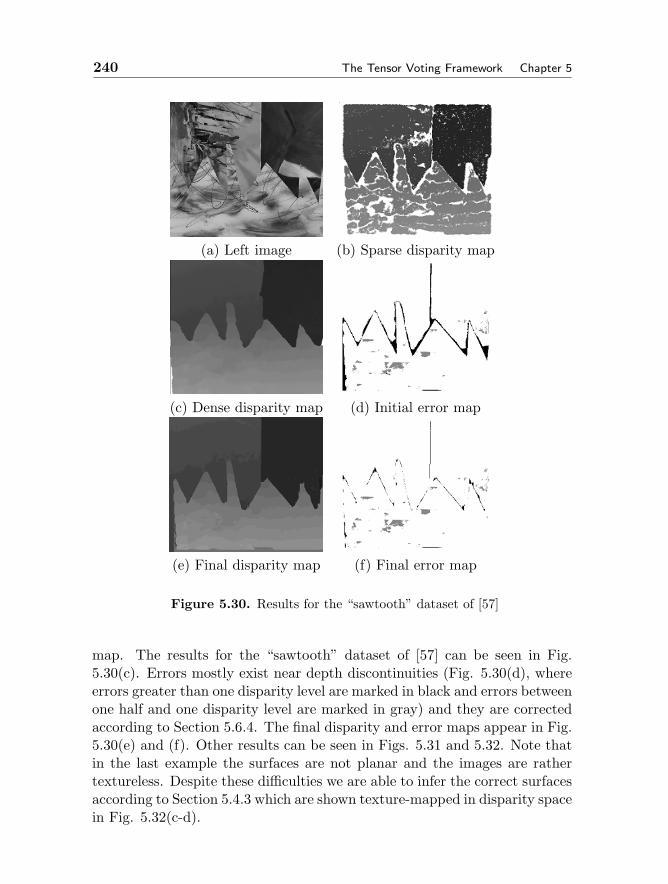
240 The Tensor Voting Framework Chapter 5
(a) Left image (b) Sparse disparity map
(c) Dense disparity map (d) Initial error map
(e) Final disparity map (f) Final error map
Figure 5.30. Results for the “sawtooth” dataset of [57]
map. The results for the “sawtooth” dataset of [57] can be seen in Fig.5.30(c). Errors mostly exist near depth discontinuities (Fig. 5.30(d), whereerrors greater than one disparity level are marked in black and errors betweenone half and one disparity level are marked in gray) and they are correctedaccording to Section 5.6.4. The final disparity and error maps appear in Fig.5.30(e) and (f). Other results can be seen in Figs. 5.31 and 5.32. Note thatin the last example the surfaces are not planar and the images are rathertextureless. Despite these difficulties we are able to infer the correct surfacesaccording to Section 5.4.3 which are shown texture-mapped in disparity spacein Fig. 5.32(c-d).
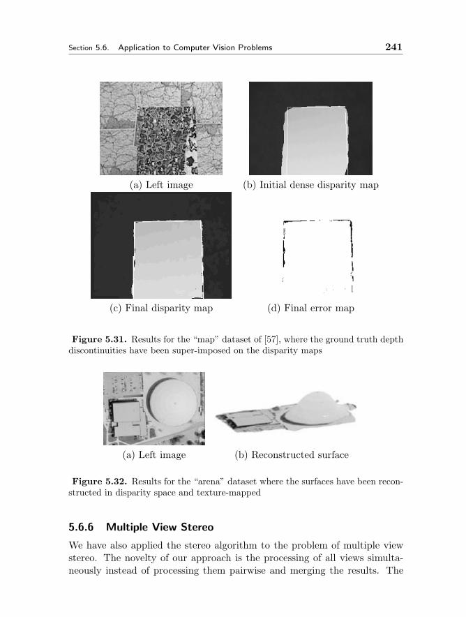
Section 5.6. Application to Computer Vision Problems 241
(a) Left image (b) Initial dense disparity map
(c) Final disparity map (d) Final error map
Figure 5.31. Results for the “map” dataset of [57], where the ground truth depthdiscontinuities have been super-imposed on the disparity maps
(a) Left image (b) Reconstructed surface
Figure 5.32. Results for the “arena” dataset where the surfaces have been recon-structed in disparity space and texture-mapped
5.6.6 Multiple View Stereo
We have also applied the stereo algorithm to the problem of multiple viewstereo. The novelty of our approach is the processing of all views simulta-neously instead of processing them pairwise and merging the results. The
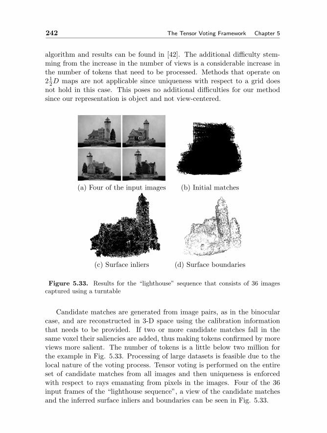
242 The Tensor Voting Framework Chapter 5
algorithm and results can be found in [42]. The additional difficulty stem-ming from the increase in the number of views is a considerable increase inthe number of tokens that need to be processed. Methods that operate on21
2D maps are not applicable since uniqueness with respect to a grid doesnot hold in this case. This poses no additional difficulties for our methodsince our representation is object and not view-centered.
(a) Four of the input images (b) Initial matches
(c) Surface inliers (d) Surface boundaries
Figure 5.33. Results for the “lighthouse” sequence that consists of 36 imagescaptured using a turntable
Candidate matches are generated from image pairs, as in the binocularcase, and are reconstructed in 3-D space using the calibration informationthat needs to be provided. If two or more candidate matches fall in thesame voxel their saliencies are added, thus making tokens confirmed by moreviews more salient. The number of tokens is a little below two million forthe example in Fig. 5.33. Processing of large datasets is feasible due to thelocal nature of the voting process. Tensor voting is performed on the entireset of candidate matches from all images and then uniqueness is enforcedwith respect to rays emanating from pixels in the images. Four of the 36input frames of the “lighthouse sequence”, a view of the candidate matchesand the inferred surface inliers and boundaries can be seen in Fig. 5.33.
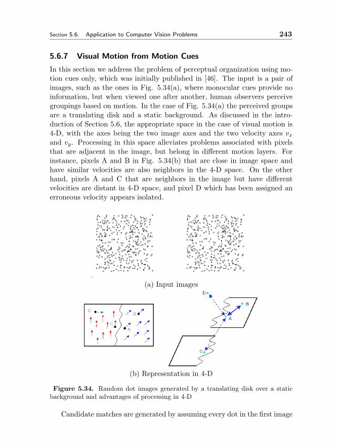
Section 5.6. Application to Computer Vision Problems 243
5.6.7 Visual Motion from Motion Cues
In this section we address the problem of perceptual organization using mo-tion cues only, which was initially published in [46]. The input is a pair ofimages, such as the ones in Fig. 5.34(a), where monocular cues provide noinformation, but when viewed one after another, human observers perceivegroupings based on motion. In the case of Fig. 5.34(a) the perceived groupsare a translating disk and a static background. As discussed in the intro-duction of Section 5.6, the appropriate space in the case of visual motion is4-D, with the axes being the two image axes and the two velocity axes vxand vy. Processing in this space alleviates problems associated with pixelsthat are adjacent in the image, but belong in different motion layers. Forinstance, pixels A and B in Fig. 5.34(b) that are close in image space andhave similar velocities are also neighbors in the 4-D space. On the otherhand, pixels A and C that are neighbors in the image but have differentvelocities are distant in 4-D space, and pixel D which has been assigned anerroneous velocity appears isolated.
(a) Input images
(b) Representation in 4-D
Figure 5.34. Random dot images generated by a translating disk over a staticbackground and advantages of processing in 4-D
Candidate matches are generated by assuming every dot in the first image
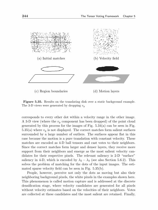
244 The Tensor Voting Framework Chapter 5
(a) Initial matches (b) Velocity field
(c) Region boundaries (d) Motion layers
Figure 5.35. Results on the translating disk over a static background example.The 3-D views were generated by dropping vy
corresponds to every other dot within a velocity range in the other image.A 3-D view (where the vy component has been dropped) of the point cloudgenerated by this process for the images of Fig. 5.34(a) can be seen in Fig.5.35(a) where vy is not displayed. The correct matches form salient surfacessurrounded by a large number of outliers. The surfaces appear flat in thiscase because the motion is a pure translation with constant velocity. Thesematches are encoded as 4-D ball tensors and cast votes to their neighbors.Since the correct matches form larger and denser layers, they receive moresupport from their neighbors and emerge as the most salient velocity can-didates for their respective pixels. The relevant saliency is 2-D “surface”saliency in 4-D, which is encoded by λ2 − λ3 (see also Section 5.6.2). Thissolves the problem of matching for the dots of the input images. The esti-mated sparse velocity field can be seen in Fig. 5.35(b).
People, however, perceive not only the dots as moving but also theirneighboring background pixels, the white pixels in the examples shown here.This phenomenon is called motion capture and is addressed at the discretedensification stage, where velocity candidates are generated for all pixelswithout velocity estimates based on the velocities of their neighbors. Votesare collected at these candidates and the most salient are retained. Finally,
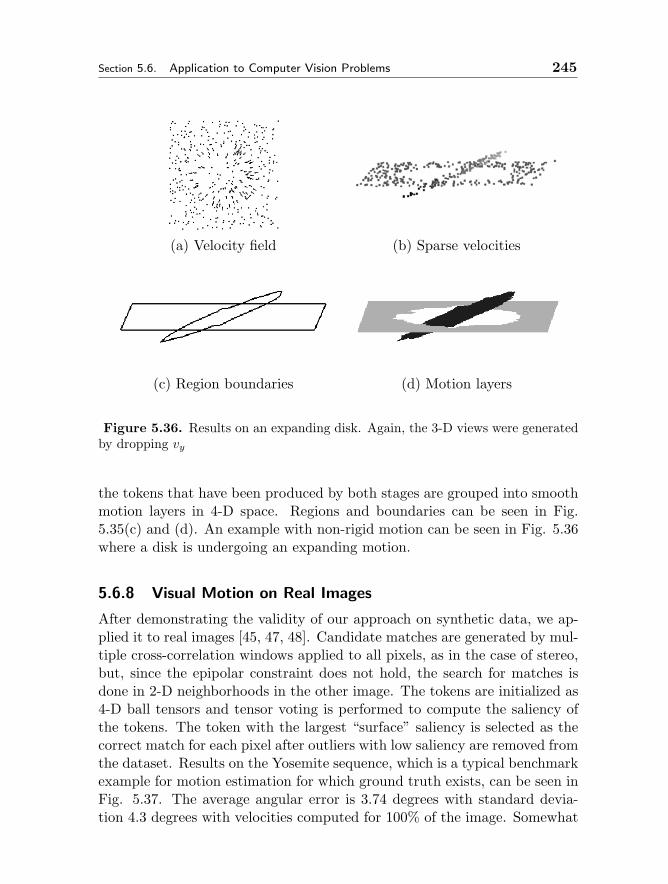
Section 5.6. Application to Computer Vision Problems 245
(a) Velocity field (b) Sparse velocities
(c) Region boundaries (d) Motion layers
Figure 5.36. Results on an expanding disk. Again, the 3-D views were generatedby dropping vy
the tokens that have been produced by both stages are grouped into smoothmotion layers in 4-D space. Regions and boundaries can be seen in Fig.5.35(c) and (d). An example with non-rigid motion can be seen in Fig. 5.36where a disk is undergoing an expanding motion.
5.6.8 Visual Motion on Real Images
After demonstrating the validity of our approach on synthetic data, we ap-plied it to real images [45, 47, 48]. Candidate matches are generated by mul-tiple cross-correlation windows applied to all pixels, as in the case of stereo,but, since the epipolar constraint does not hold, the search for matches isdone in 2-D neighborhoods in the other image. The tokens are initialized as4-D ball tensors and tensor voting is performed to compute the saliency ofthe tokens. The token with the largest “surface” saliency is selected as thecorrect match for each pixel after outliers with low saliency are removed fromthe dataset. Results on the Yosemite sequence, which is a typical benchmarkexample for motion estimation for which ground truth exists, can be seen inFig. 5.37. The average angular error is 3.74 degrees with standard devia-tion 4.3 degrees with velocities computed for 100% of the image. Somewhat
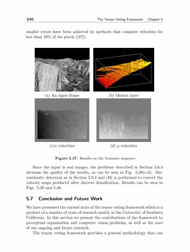
246 The Tensor Voting Framework Chapter 5
smaller errors have been achieved by methods that compute velocities forless than 10% of the pixels ([47]).
(a) An input frame (b) Motion layer
(c)x velocities (d) y velocities
Figure 5.37. Results on the Yosemite sequence
Since the input is real images, the problems described in Section 5.6.4decrease the quality of the results, as can be seen in Fig. 5.38(c-d). Dis-continuity detection as in Section 5.6.4 and [48] is performed to correct thevelocity maps produced after discrete densification. Results can be seen inFigs. 5.39 and 5.40.
5.7 Conclusion and Future Work
We have presented the current state of the tensor voting framework which is aproduct of a number of years of research mostly at the University of SouthernCalifornia. In this section we present the contributions of the framework toperceptual organization and computer vision problems, as well as the axesof our ongoing and future research.
The tensor voting framework provides a general methodology that can
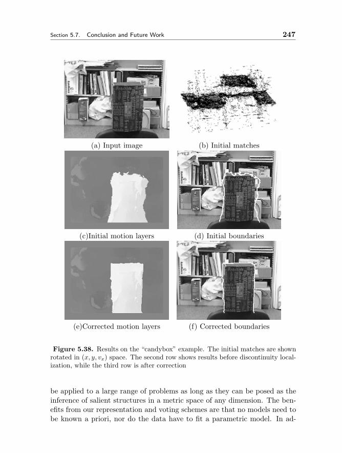
Section 5.7. Conclusion and Future Work 247
(a) Input image (b) Initial matches
(c)Initial motion layers (d) Initial boundaries
(e)Corrected motion layers (f) Corrected boundaries
Figure 5.38. Results on the “candybox” example. The initial matches are shownrotated in (x, y, vx) space. The second row shows results before discontinuity local-ization, while the third row is after correction
be applied to a large range of problems as long as they can be posed as theinference of salient structures in a metric space of any dimension. The ben-efits from our representation and voting schemes are that no models need tobe known a priori, nor do the data have to fit a parametric model. In ad-
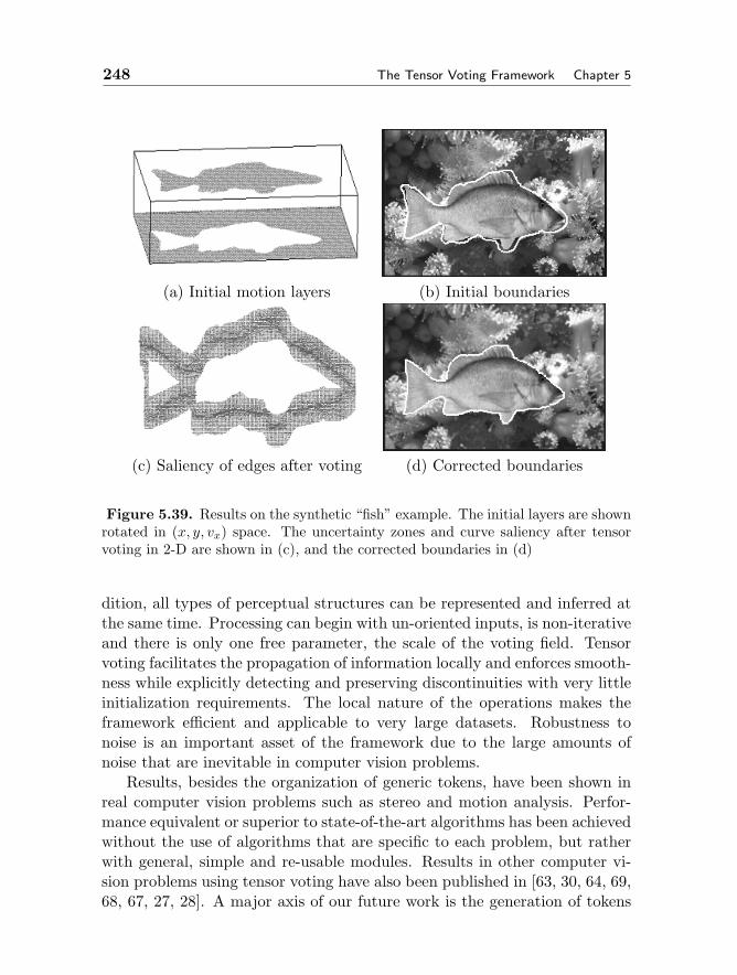
248 The Tensor Voting Framework Chapter 5
(a) Initial motion layers (b) Initial boundaries
(c) Saliency of edges after voting (d) Corrected boundaries
Figure 5.39. Results on the synthetic “fish” example. The initial layers are shownrotated in (x, y, vx) space. The uncertainty zones and curve saliency after tensorvoting in 2-D are shown in (c), and the corrected boundaries in (d)
dition, all types of perceptual structures can be represented and inferred atthe same time. Processing can begin with un-oriented inputs, is non-iterativeand there is only one free parameter, the scale of the voting field. Tensorvoting facilitates the propagation of information locally and enforces smooth-ness while explicitly detecting and preserving discontinuities with very littleinitialization requirements. The local nature of the operations makes theframework efficient and applicable to very large datasets. Robustness tonoise is an important asset of the framework due to the large amounts ofnoise that are inevitable in computer vision problems.
Results, besides the organization of generic tokens, have been shown inreal computer vision problems such as stereo and motion analysis. Perfor-mance equivalent or superior to state-of-the-art algorithms has been achievedwithout the use of algorithms that are specific to each problem, but ratherwith general, simple and re-usable modules. Results in other computer vi-sion problems using tensor voting have also been published in [63, 30, 64, 69,68, 67, 27, 28]. A major axis of our future work is the generation of tokens
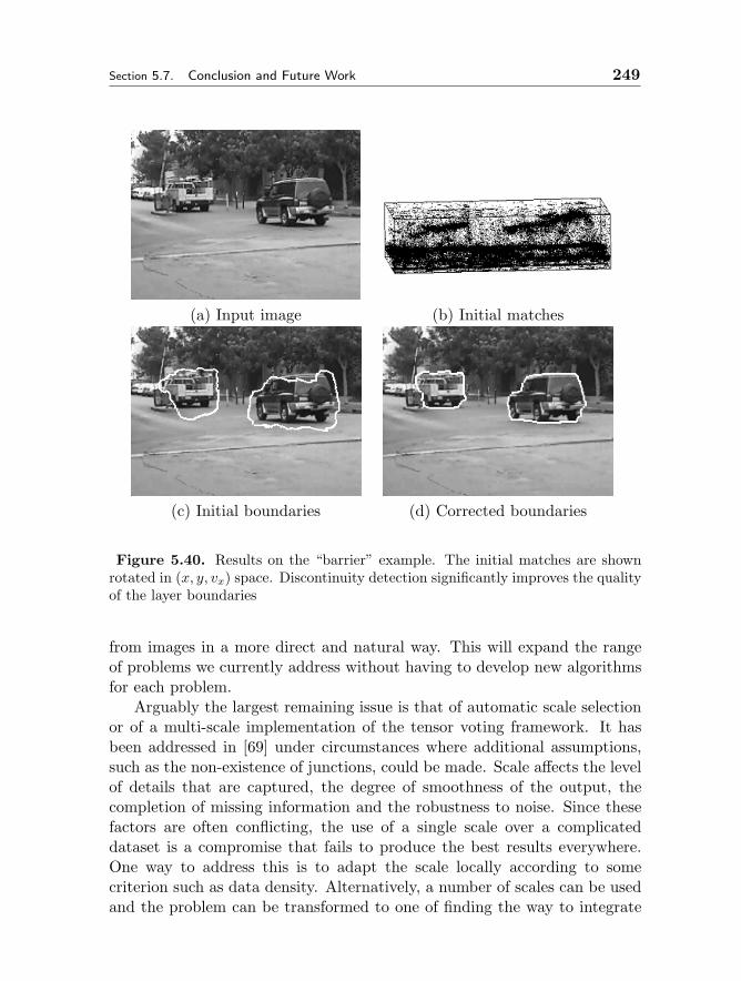
Section 5.7. Conclusion and Future Work 249
(a) Input image (b) Initial matches
(c) Initial boundaries (d) Corrected boundaries
Figure 5.40. Results on the “barrier” example. The initial matches are shownrotated in (x, y, vx) space. Discontinuity detection significantly improves the qualityof the layer boundaries
from images in a more direct and natural way. This will expand the rangeof problems we currently address without having to develop new algorithmsfor each problem.
Arguably the largest remaining issue is that of automatic scale selectionor of a multi-scale implementation of the tensor voting framework. It hasbeen addressed in [69] under circumstances where additional assumptions,such as the non-existence of junctions, could be made. Scale affects the levelof details that are captured, the degree of smoothness of the output, thecompletion of missing information and the robustness to noise. Since thesefactors are often conflicting, the use of a single scale over a complicateddataset is a compromise that fails to produce the best results everywhere.One way to address this is to adapt the scale locally according to somecriterion such as data density. Alternatively, a number of scales can be usedand the problem can be transformed to one of finding the way to integrate
250 The Tensor Voting Framework Chapter 5
the results over the different scales. A fine to coarse scheme was adopted in[69], which is consistent with the majority of the literature, but one couldenvision coarse to fine schemes as well. In any case, the issue remains openand is further complicated by that fact that even human perception is afunction of scale.
5.8 Acknowledgment
The authors would like to thank all those who contributed to the researchin tensor voting at the University of Southern California. From the orig-inal vector voting scheme of Gideon Guy, to the first implementation ofthe framework as presented in [40] by Chi-Keung Tang and Mi Suen Lee,to the other contributors: Pierre Kornprobst, Amin Massad, Lee Gaucher,Mircea Nicolescu, Eun-Young Kang, Jinman Kang, Rene Dencker Eriksen,Wai-Shun Tong.
Bibliography
[1] S. Arya, D.M. Mount, N.S. Netanyahu, R. Silverman, and A.Y. Wu. An optimalalgorithm for approximate nearest neighbor searching fixed dimensions. Journalof the ACM, 45(6):891–923, 1998.
[2] J.D. Boissonnat. Representing 2d and 3d shapes with the delaunay triangula-tion. In ICPR84, pages 745–748, 1984.
[3] Y. Boykov, O. Veksler, and R. Zabih. Fast approximate energy minimizationvia graph cuts. PAMI, 23(11):1222–1239, November 2001.
[4] H. Chen, P. Meer, and D.E. Tyler. Robust regression for data with multiplestructures. In CVPR01, pages I:1069–1075, 2001.
[5] K.J. Cho and P. Meer. Image segmentation from consensus information. CVIU,68(1):72–89, October 1997.
[6] J. Dolan and E.M. Riseman. Computing curvilinear structure by token-basedgrouping. In CVPR92, pages 264–270, 1992.
[7] H. Edelsbrunner and E.P. Mucke. Three-dimensional alpha shapes. ACMTransactions on Graphics, 13(1):43–72, 1994.
[8] O.D. Faugeras and M. Berthod. Improving consistency and reducing ambiguityin stochastic labeling: An optimization approach. PAMI, 3(4):412–424, July1981.
[9] M.A. Fischler and R.C. Bolles. Random sample consensus: A paradigm formodel fitting with applications to image analysis and automated cartography.Comm. of the ACM, 24(6):381–395, 1981.
[10] Y. Gdalyahu, D. Weinshall, and M. Werman. Self-organization in vision:Stochastic clustering for image segmentation, perceptual grouping, and imagedatabase organization. PAMI, 23(10):1053–1074, October 2001.
[11] S. Geman and D. Geman. Stochastic relaxation, gibbs distributions, and thebayesian restoration of images. PAMI, 6(6):721–741, November 1984.
Bibliography 251
[12] G.H. Granlund and H. Knutsson. Signal Processing for Computer Vision.Kluwer, December 1995.
[13] S. Grossberg and E. Mingolla. Neural dynamics of form perception: Boundarycompletion. Psychological Review, pages 173–211, 1985.
[14] S. Grossberg and D. Todorovic. Neural dynamics of 1-d and 2-d brightnessperception: A unified model of classical and recent phenomena. Perception andPsychophysics, 43:723–742, 1988.
[15] G. Guy and G. Medioni. Inferring global perceptual contours from local fea-tures. IJCV, 20(1/2):113–133, 1996.
[16] G. Guy and G. Medioni. Inference of surfaces, 3d curves, and junctions fromsparse, noisy, 3d data. PAMI, 19(11):1265–1277, November 1997.
[17] R.M. Haralick and L.G. Shapiro. The consistent labeling problem: Part i.PAMI, 1(2):173–184, April 1979.
[18] R.M. Haralick and L.G. Shapiro. The consistent labeling problem: Part ii.PAMI, 2(3):193–203, May 1980.
[19] F. Heitger and R. von der Heydt. A computational model of neural contourprocessing: Figure-ground segregation and illusory contours. In ICCV93, pages32–40, 1993.
[20] S. Osher H.K. Zhao and R. Fedkiw. Fast surface reconstruction using the levelset method. In UCLA Computational and Applied Mathematics Reports, pages32–40, 2001.
[21] H. Hoppe, T. DeRose, T. Duchamp, J. McDonald, and W. Stuetzle. Surfacereconstruction from unorganized points. Computer Graphics, 26(2):71–78, 1992.
[22] B.K.P. Horn and B.G. Schunck. Determining optical flow. AI, 17(1-3):185–203,August 1981.
[23] P.V.C. Hough. Method and means for recognizing complex patterns. In USPatent, 1962.
[24] R.A. Hummel and S.W. Zucker. On the foundations of relaxation labelingprocesses. PAMI, 5(3):267–287, May 1983.
[25] D.W. Jacobs. Robust and efficient detection of salient convex groups. PAMI,18(1):23–37, January 1996.
[26] A.K. Jain and R.C. Dubes. Algorithms for clustering data. In Prentice-Hall,1988.
[27] J. Jia and C.K. Tang. Image repairing: Robust image synthesis by adaptive ndtensor voting. In CVPR03, pages I:643–650, 2003.
[28] J. Kang, I. Cohen, and G. Medioni. Continuous tracking within and acrosscamera streams. In CVPR03, pages I:267–272, 2003.
[29] G.K. Kanizsa. Subjective contours. In Scientific American, volume 234, pages48–54, 1976.
[30] P. Kornprobst and G. Medioni. Tracking segmented objects using tensor voting.In CVPR00, pages II: 118–125, 2000.
[31] K. Koster and M. Spann. Mir: An approach to robust clustering-applicationto range image segmentation. PAMI, 22(5):430–444, May 2000.
[32] Y.G. Leclerc. Constructing simple stable descriptions for image partitioning.IJCV, 3(1):73–102, May 1989.

252 The Tensor Voting Framework Chapter 5
[33] K.M. Lee, P. Meer, and R.H. Park. Robust adaptive segmentation of rangeimages. PAMI, 20(2):200–205, February 1998.
[34] M.S. Lee and G. Medioni. Inferring segmented surface description from stereodata. In CVPR98, pages 346–352, 1998.
[35] M.S. Lee, G. Medioni, and P. Mordohai. Inference of segmented overlappingsurfaces from binocular stereo. PAMI, 24(6):824–837, June 2002.
[36] Z. Li. A neural model of contour integration in the primary visual cortex.Neural Computation, 10:903–940, 1998.
[37] W.E. Lorensen and H.E. Cline. Marching cubes: A high resolution 3d surfacereconstruction algorithm. Computer Graphics, 21(4):163–169, 1987.
[38] D.G. Lowe. Perceptual Organization and Visual Recognition. Kluwer, June1985.
[39] D. Marr. Vision. Freeman Press, 1982.[40] G. Medioni, M.S. Lee, and C.K. Tang. A Computational Framework for Seg-
mentation and Grouping. Elsevier, 2000.[41] R. Mohan and R. Nevatia. Perceptual organization for scene segmentation and
description. PAMI, 14(6):616–635, June 1992.[42] P. Mordohai and G. Medioni. Perceptual grouping for multiple view stereo
using tensor voting. In ICPR02, pages III: 639–644, 2002.[43] J.M. Morel and S. Solimini. Variational Methods in Image Segmentation.
Birkhauser, 1995.[44] H. Neummann and E. Mingolla. Computational neural models of spatial in-
tegration in perceptual grouping. From Fragments to Objects: Grouping andSegmentation in Vision, T.F.Shipley and P.J. Kellman, Editors, pages 353–400,2001.
[45] M. Nicolescu and G. Medioni. 4-d voting for matching, densification and seg-mentation into motion layers. In ICPR02, pages III: 303–308, 2002.
[46] M. Nicolescu and G. Medioni. Perceptual grouping from motion cues usingtensor voting in 4-d. In ECCV02, pages III: 423–428, 2002.
[47] M. Nicolescu and G. Medioni. Layered 4d representation and voting for group-ing from motion. PAMI, 25(4):492–501, April 2003.
[48] M. Nicolescu and G. Medioni. Motion segmentation with accurate boundaries- a tensor voting approach. In CVPR03, pages I:382–389, 2003.
[49] S. Osher and R.P. Fedkiw. The Level Set Method and Dynamic Implicit Sur-faces. Springer Verlag, 2002.
[50] P. Parent and S.W. Zucker. Trace inference, curvature consistency, and curvedetection. PAMI, 11(8):823–839, August 1989.
[51] T.A. Poggio, V. Torre, and C. Koch. Computational vision and regularizationtheory. Nature, 317:314–319, 1985.
[52] L. Robert and R. Deriche. Dense depth map reconstruction: A minimizationand regularization approach which preserves discontinuities. In ECCV96, pagesI:439–451, 1996.
[53] A. Robles-Kelly and E.R. Hancock. An expectation-maximisation frameworkfor perceptual grouping. In IWVF4, LNCS 2059, pages 594–605. SpringerVerlag, 2001.
Bibliography 253
[54] P.T. Sander and S.W. Zucker. Inferring surface trace and differential structurefrom 3-d images. PAMI, 12(9):833–854, September 1990.
[55] S. Sarkar and K.L. Boyer. A computational structure for preattentive per-ceptual organization: Graphical enumeration and voting methods. SMC, 24:246–267, 1994.
[56] E. Saund. Labeling of curvilinear structure across scales by token grouping. InCVPR92, pages 257–263, 1992.
[57] D. Scharstein and R. Szeliski. A taxonomy and evaluation of dense two-framestereo correspondence algorithms. IJCV, 47(1-3):7–42, April 2002.
[58] J.A. Sethian. Level Set Methods: Evolving Interfaces in Geometry, Fluid Me-chanics, Computer Vision and Materials Science. Cambridge University Press,1996.
[59] A. Shashua and S. Ullman. Structural saliency: The detection of globally salientstructures using a locally connected network. In ICCV88, pages 321–327, 1988.
[60] J. Shi and J. Malik. Normalized cuts and image segmentation. PAMI, 22(8):888–905, August 2000.
[61] R. Szeliski, D. Tonnesen, and D. Terzopoulos. Modeling surfaces of arbitrarytopology with dynamic particles. In CVPR93, pages 82–87, 1993.
[62] C.K. Tang and G. Medioni. Inference of integrated surface, curve, and junctiondescriptions from sparse 3d data. PAMI, 20(11):1206–1223, November 1998.
[63] C.K. Tang, G. Medioni, and M.S. Lee. Epipolar geometry estimation by tensorvoting in 8d. In ICCV99, pages 502–509, 1999.
[64] C.K. Tang, G. Medioni, and M.S. Lee. N-dimensional tensor voting and appli-cation to epipolar geometry estimation. PAMI, 23(8):829–844, August 2001.
[65] D. Terzopoulos. Regularization of inverse visual problems involving discontinu-ities. PAMI, 8(4):413–424, July 1986.
[66] D. Terzopoulos and D. Metaxas. Dynamic 3d models with local and globaldeformations: Deformable superquadrics. PAMI, 13(7):703–714, July 1991.
[67] W.S. Tong and C.K. Tang. Rod-tv: Reconstruction on demand by tensorvoting. In CVPR03, pages II:391–398, 2003.
[68] W.S. Tong, C.K. Tang, and G. Medioni. Epipolar geometry estimation fornon-static scenes by 4d tensor voting. In CVPR01, pages I:926–933, 2001.
[69] W.S. Tong, C.K. Tang, and G. Medioni. First order tensor voting and applica-tion to 3-d scale analysis. In CVPR01, pages I:175–182, 2001.
[70] M. Wertheimer. Laws of organization in perceptual forms. PsycologischeForschung, Translation by W. Ellis, A source book of Gestalt psychology (1938),4:301–350, 1923.
[71] C.F. Westin. A Tensor Framework for Multidimensional Signal Processing.Ph.D. thesis, Linkoeping University, Sweden,, 1994.
[72] L.R. Williams and D.W. Jacobs. Stochastic completion fields: A neural modelof illusory contour shape and salience. Neural Computation, 9(4):837–858, 1997.
[73] S.C. Yen and L.H. Finkel. Extraction of perceptually salient contours by striatecortical networks. Vision Research, 38(5):719–741, 1998.
[74] X.M. Yu, T.D. Bui, and A. Krzyzak. Robust estimation for range image seg-mentation and reconstruction. PAMI, 16(5):530–538, May 1994.

SECTION II:APPLICATIONS INCOMPUTER VISION
The chapters in this section describe a variety of interesting applicationsin computer vision, ranging from the more traditional (content-based im-age retrieval, face detection, human tracking) to the more graphics-oriented(image-based lighting and visual effects).
In Chapter 6, Debevec describes how scenes and objects can be illu-minated using images of light from the real world. While this operation,also known as image-based lighting, has its roots in computer graphics, itrequires computer vision techniques to extract high dynamic range imagesand resample the captured light.
Many of the special effects seen in movies rely on computer vision tech-niques to facilitate their production. In Chapter 7, Roble describes some ofvision techniques that have been used successfully in the movie industry.
A natural extension to current text-based search engines would be imageretrieval. In Chapter 8, Gevers and Smeulders present a survey on the theoryand techniques for content-based image retrieval. The issues covered includeinteractive query formulation, image feature extraction, representation andindexing, search techniques, and learning based on feedback.
Li and Lu describe techniques for face detection, alignment, and recog-nition in Chapter 9. They show how the difficult problems of changing headpose and different illumination can be handled.
In Chapter 10, Turk and Kolsch describe the area of perceptual interfaces,which involves the use of multiple perceptual modalities (e.g., vision, speech,haptic) to enable human-machine interaction. The authors motivate the needfor such a study and discuss issues related to vision-based interfaces.254
Chapter 6
IMAGE-BASED LIGHTING
Paul E. Debevec
Image-based lighting (IBL) is the process of illuminating scenes and ob-jects - be they real or synthetic - with images of light from the real world.IBL evolved from the techniques known as environment mapping and re-flection mapping [3], [20], in which panoramic images are used as texturemaps on computer generated models to show shiny objects reflecting realand synthetic environments. When used effectively, image-based lightingcan produce highly realistic renderings of people, objects, and environments,and it can be used to convincingly integrate computer generated objects intoreal world scenes.
The basic steps in image-based lighting are:
1. Capturing real-world illumination as an omnidirectional, high dynamicrange image
2. Mapping the illumination on to a representation of the environment
3. Placing the 3D object inside the environment
4. Simulating the light from the environment illuminating the CG object
Figure 6.1 shows an example of an object illuminated entirely using IBL.The light was captured in a kitchen, and includes light from the fixture on theceiling, the blue sky from the windows, and the indirect light from the walls,ceiling, and cabinets in the room. The light from this room was mapped ontoa large sphere, and the model of the microscope on the table was placed inthe middle of the sphere. Then, a global illumination renderer was used tosimulate the object’s appearance as illuminated by the light coming from the
255
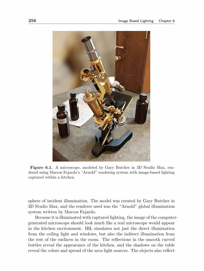
256 Image Based Lighting Chapter 6
Figure 6.1. A microscope, modeled by Gary Butcher in 3D Studio Max, ren-dered using Marcos Fajardo’s “Arnold” rendering system with image-based lightingcaptured within a kitchen.
sphere of incident illumination. The model was created by Gary Butcher in3D Studio Max, and the renderer used was the “Arnold” global illuminationsystem written by Marcos Fajardo.
Because it is illuminated with captured lighting, the image of the computer-generated microscope should look much like a real microscope would appearin the kitchen environment. IBL simulates not just the direct illuminationfrom the ceiling light and windows, but also the indirect illumination fromthe rest of the surfaces in the room. The reflections in the smooth curvedbottles reveal the appearance of the kitchen, and the shadows on the tablereveal the colors and spread of the area light sources. The objects also reflect
Section 6.1. Basic Image Based Lighting 257
each other, owing to the ray-tracing component of the global illuminationtechniques being employed.
This first part of this chapter will describe the theory and practice ofimage-based lighting, and will provide concrete examples of the technique inaction using Greg Ward’s Radiance lighting simulation system. The secondpart of the chapter will present advanced image-based lighting techniques,such as having the objects cast shadows into the scene, and capturing light-ing that varies within space. The final part of this chapter will discussimage-based relighting, which is the process of synthetically illuminatingreal objects and people with light captured from the real world.
6.1 Basic Image-Based Lighting
6.1.1 Capturing Light
The first step of image-based lighting is to obtain a measurement of real-world illumination, called a light probe image in [7]. Several such imagesavailable in the Light Probe Image Gallery at http://www.debevec.org/Probes/.The web site includes the kitchen environment used to render the microscopeas well as lighting captured in various other interior and outdoor environ-ments. A few of these environments are shown in Figure 6.2.
Light Probe images are photographically acquired images of the realworld with two important properties: first, they are omnidirectional - forevery direction in the world, there is a pixel in the image that correspondsto that direction. Second, their pixel values are linearly proportional to theamount of light in the real world. The rest of this section will describetechniques for how to take images satisfying both of these properties.
Taking omnidirectional images can be done in a number of ways. Thesimplest way is to use a regular camera to take a photograph of a mirroredball placed in a scene. A mirrored ball actually reflects the entire worldaround it, not just the hemisphere toward the camera: light rays reflectingoff the outer circumference of the ball glance toward the camera from the backhalf of the environment. Another method to obtain omnidirectional imagesusing is to shoot a mosaic of many pictures looking in different directions[4, 26] and combine them using an image stitching program such as RealVizStitcher. A good way to cover a particularly large area in each shot is touse a fisheye lens [14], allowing the full field to be covered in as few as twoimages. A final technique is to use a special scanning panoramic camera,such as ones made by Panoscan or Spheron, which uses a vertical row ofCCD elements on a rotating camera head to scan across 360 degrees field of
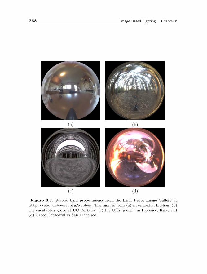
258 Image Based Lighting Chapter 6
(a) (b)
(c) (d)
Figure 6.2. Several light probe images from the Light Probe Image Gallery athttp://www.debevec.org/Probes. The light is from (a) a residential kitchen, (b)the eucalyptus grove at UC Berkeley, (c) the Uffizi gallery in Florence, Italy, and(d) Grace Cathedral in San Francisco.
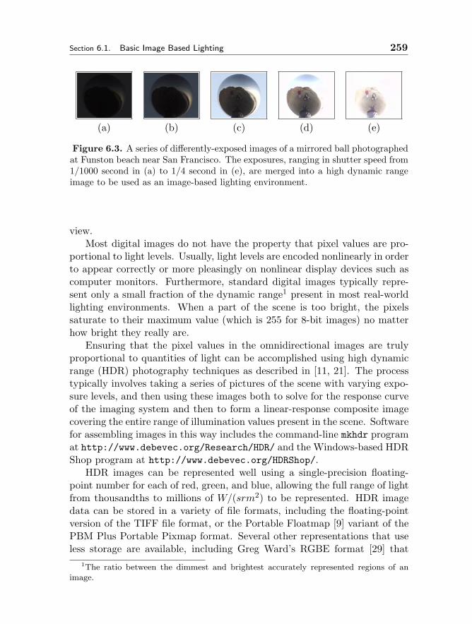
Section 6.1. Basic Image Based Lighting 259
(a) (b) (c) (d) (e)
Figure 6.3. A series of differently-exposed images of a mirrored ball photographedat Funston beach near San Francisco. The exposures, ranging in shutter speed from1/1000 second in (a) to 1/4 second in (e), are merged into a high dynamic rangeimage to be used as an image-based lighting environment.
view.Most digital images do not have the property that pixel values are pro-
portional to light levels. Usually, light levels are encoded nonlinearly in orderto appear correctly or more pleasingly on nonlinear display devices such ascomputer monitors. Furthermore, standard digital images typically repre-sent only a small fraction of the dynamic range1 present in most real-worldlighting environments. When a part of the scene is too bright, the pixelssaturate to their maximum value (which is 255 for 8-bit images) no matterhow bright they really are.
Ensuring that the pixel values in the omnidirectional images are trulyproportional to quantities of light can be accomplished using high dynamicrange (HDR) photography techniques as described in [11, 21]. The processtypically involves taking a series of pictures of the scene with varying expo-sure levels, and then using these images both to solve for the response curveof the imaging system and then to form a linear-response composite imagecovering the entire range of illumination values present in the scene. Softwarefor assembling images in this way includes the command-line mkhdr programat http://www.debevec.org/Research/HDR/ and the Windows-based HDRShop program at http://www.debevec.org/HDRShop/.
HDR images can be represented well using a single-precision floating-point number for each of red, green, and blue, allowing the full range of lightfrom thousandths to millions of W/(srm2) to be represented. HDR imagedata can be stored in a variety of file formats, including the floating-pointversion of the TIFF file format, or the Portable Floatmap [9] variant of thePBM Plus Portable Pixmap format. Several other representations that useless storage are available, including Greg Ward’s RGBE format [29] that
1The ratio between the dimmest and brightest accurately represented regions of animage.
260 Image Based Lighting Chapter 6
uses one byte for each of red, green, blue, and a common 8-bit exponent,and Ward’s more recent 24-bit and 32-bit LogLuv formats recently includedin the TIFF standard [18]. The light probe images in the light probe imagegallery are available in the RGBE format, allowing them to be easily used inWard’s RADIANCE global illumination renderer. We’ll see how to do thisin the next section.
Figure 6.3 shows a series of images used in creating a light probe image.To acquire these images, a three-inch polished ball bearing was placed ontop of a tripod at Funston Beach near San Francisco, and a digital camerawith a telephoto zoom lens was used to take a series of exposures of the ball.Being careful not to disturb the camera, pictures were taken at shutter speedsranging from 1/4 second to 1/10000 second, allowing the camera to properlyimage everything from the dark cliffs to the bright sky and the setting sun.The images were assembled using code similar to that now found in mkhdrand HDR Shop, yielding a high dynamic range, linear-response image.
6.1.2 Illuminating Synthetic Objects with Real Light
Image-based lighting is the process of using light probe images as sourcesof illumination for CG scenes and objects. IBL is now supported by severalcommercial renderers, including LightWave 3D, Entropy, and Final Render.For this tutorial, we’ll use the freely-downloadable RADIANCE lighting sim-ulation package written by Greg Ward at Lawrence Berkeley Laboratories.RADIANCE is a UNIX package, which means that to use it you’ll need touse a computer such as a PC running Linux or a Silicon Graphics or Sunworkstation. Here are the steps to using image-based lighting to illuminatesynthetic objects in RADIANCE:
1. Download and install RADIANCE
First, test to see if you already have RADIANCE installed by typingwhich rpict at a UNIX command prompt. If the shell returns “Com-mand not found”, you’ll need to install RADIANCE. To do this, visitthe RADIANCE web site at http://radsite.lbl.gov/radiance andclick on the “download” option. As of this writing, the current versionis 3.1.8, and it is pre-compiled for SGI and Sun workstations. For otheroperating systems, such as Linux, you can download the source filesand then compile the executable programs using the makeall script.Once installed, make sure that the RADIANCE binary directory is inyour $PATH and that your $RAYPATH environment variable includes theRADIANCE library directory. Your system administrator should be
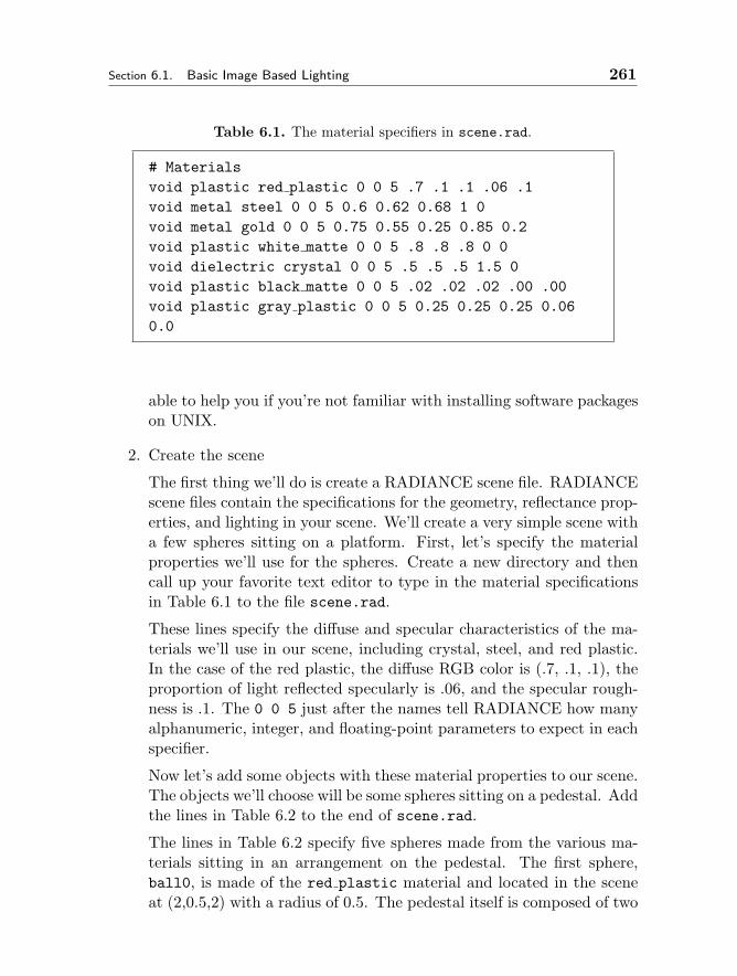
Section 6.1. Basic Image Based Lighting 261
Table 6.1. The material specifiers in scene.rad.
# Materialsvoid plastic red plastic 0 0 5 .7 .1 .1 .06 .1void metal steel 0 0 5 0.6 0.62 0.68 1 0void metal gold 0 0 5 0.75 0.55 0.25 0.85 0.2void plastic white matte 0 0 5 .8 .8 .8 0 0void dielectric crystal 0 0 5 .5 .5 .5 1.5 0void plastic black matte 0 0 5 .02 .02 .02 .00 .00void plastic gray plastic 0 0 5 0.25 0.25 0.25 0.060.0
able to help you if you’re not familiar with installing software packageson UNIX.
2. Create the scene
The first thing we’ll do is create a RADIANCE scene file. RADIANCEscene files contain the specifications for the geometry, reflectance prop-erties, and lighting in your scene. We’ll create a very simple scene witha few spheres sitting on a platform. First, let’s specify the materialproperties we’ll use for the spheres. Create a new directory and thencall up your favorite text editor to type in the material specificationsin Table 6.1 to the file scene.rad.
These lines specify the diffuse and specular characteristics of the ma-terials we’ll use in our scene, including crystal, steel, and red plastic.In the case of the red plastic, the diffuse RGB color is (.7, .1, .1), theproportion of light reflected specularly is .06, and the specular rough-ness is .1. The 0 0 5 just after the names tell RADIANCE how manyalphanumeric, integer, and floating-point parameters to expect in eachspecifier.
Now let’s add some objects with these material properties to our scene.The objects we’ll choose will be some spheres sitting on a pedestal. Addthe lines in Table 6.2 to the end of scene.rad.
The lines in Table 6.2 specify five spheres made from the various ma-terials sitting in an arrangement on the pedestal. The first sphere,ball0, is made of the red plastic material and located in the sceneat (2,0.5,2) with a radius of 0.5. The pedestal itself is composed of two
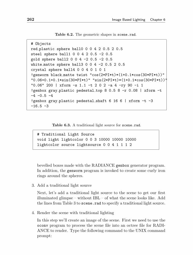
262 Image Based Lighting Chapter 6
Table 6.2. The geometric shapes in scene.rad.
# Objectsred plastic sphere ball0 0 0 4 2 0.5 2 0.5steel sphere ball1 0 0 4 2 0.5 -2 0.5gold sphere ball2 0 0 4 -2 0.5 -2 0.5white matte sphere ball3 0 0 4 -2 0.5 2 0.5crystal sphere ball4 0 0 4 0 1 0 1!genworm black matte twist "cos(2*PI*t)*(1+0.1*cos(30*PI*t))""0.06+0.1+0.1*sin(30*PI*t)" "sin(2*PI*t)*(1+0.1*cos(30*PI*t))""0.06" 200 | xform -s 1.1 -t 2 0 2 -a 4 -ry 90 -i 1!genbox gray plastic pedestal top 8 0.5 8 -r 0.08 | xform -t-4 -0.5 -4!genbox gray plastic pedestal shaft 6 16 6 | xform -t -3-16.5 -3
Table 6.3. A traditional light source for scene.rad.
# Traditional Light Sourcevoid light lightcolor 0 0 3 10000 10000 10000lightcolor source lightsource 0 0 4 1 1 1 2
bevelled boxes made with the RADIANCE genbox generator program.In addition, the genworm program is invoked to create some curly ironrings around the spheres.
3. Add a traditional light source
Next, let’s add a traditional light source to the scene to get our firstilluminated glimpse – without IBL – of what the scene looks like. Addthe lines from Table 3 to scene.rad to specify a traditional light source.
4. Render the scene with traditional lighting
In this step we’ll create an image of the scene. First we need to use theoconv program to process the scene file into an octree file for RADI-ANCE to render. Type the following command to the UNIX commandprompt:
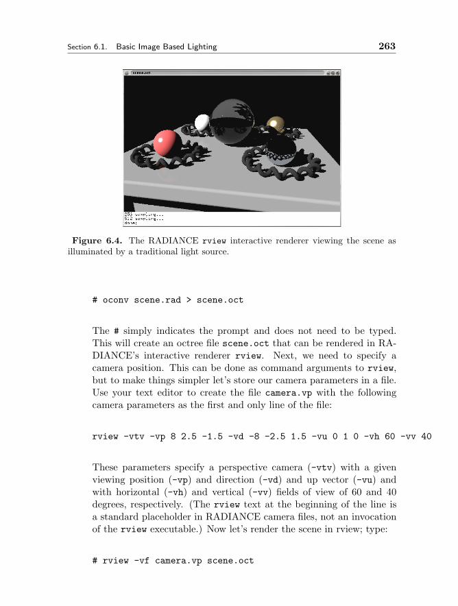
Section 6.1. Basic Image Based Lighting 263
Figure 6.4. The RADIANCE rview interactive renderer viewing the scene asilluminated by a traditional light source.
# oconv scene.rad > scene.oct
The # simply indicates the prompt and does not need to be typed.This will create an octree file scene.oct that can be rendered in RA-DIANCE’s interactive renderer rview. Next, we need to specify acamera position. This can be done as command arguments to rview,but to make things simpler let’s store our camera parameters in a file.Use your text editor to create the file camera.vp with the followingcamera parameters as the first and only line of the file:
rview -vtv -vp 8 2.5 -1.5 -vd -8 -2.5 1.5 -vu 0 1 0 -vh 60 -vv 40
These parameters specify a perspective camera (-vtv) with a givenviewing position (-vp) and direction (-vd) and up vector (-vu) andwith horizontal (-vh) and vertical (-vv) fields of view of 60 and 40degrees, respectively. (The rview text at the beginning of the line isa standard placeholder in RADIANCE camera files, not an invocationof the rview executable.) Now let’s render the scene in rview; type:
# rview -vf camera.vp scene.oct
264 Image Based Lighting Chapter 6
In a few seconds, you should get an image window similar to whatis shown in Figure 4. The image shows the spheres on the platform,surrounded by the curly rings, and illuminated by the traditional lightsource. The image may or may not be pleasing, but it certainly looksvery computer-generated. Let’s now see if we can make it more realisticby lighting the scene with image-based lighting.
5. Download a light probe image
Visit the Light Probe Image Gallery at http://www.debevec.org/Probes/and choose a light probe image to download. The light probe imageswithout concentrated light sources tend to produce good-quality ren-ders more quickly, so using one of the “beach”, “uffizi”, or “kitchen”probes to begin is recommended. We’ll choose the “beach” probe de-scribed earlier in our first example. Download the beach probe.hdrfile to your computer by shift-clicking or right-clicking “Save TargetAs...” or “Save Link As...” and then view it using the RADIANCEimage viewer ximage:
# ximage beach_probe.hdr
If the probe downloaded properly, a window should pop up displayingthe beach probe image. While the window is up you can click-dragthe mouse pointer over a region of the image and then press “=” tore-expose the image to properly display the region of interest. If theimage did not download properly, try downloading and expanding theall probes.zip or all probes.tar.gz archive from the same webpage, which will download all the light probes images and ensure thattheir binary format is preserved. When you’re done examining thelight probe image, press the “q” key in the ximage window to dismissthe window.
6. Map the light probe image onto the environment
Let’s now add the light probe image to our scene by mapping it ontoan environment surrounding our objects. First, we need to create anew file that will specify the mathematical formula for mapping thelight probe image onto the environment. Use your text editor to createthe file angmap.cal containing the lines from Table 6.
This file will tell RADIANCE how to map direction vectors in the world(Dx, Dy, Dz) into light probe image coordinates (u,v). Fortunately,
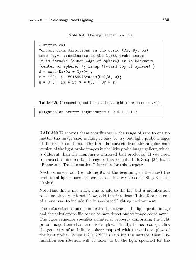
Section 6.1. Basic Image Based Lighting 265
Table 6.4. The angular map .cal file.
angmap.calConvert from directions in the world (Dx, Dy, Dz)into (u,v) coordinates on the light probe image-z is forward (outer edge of sphere) +z is backward(center of sphere) +y is up (toward top of sphere) d = sqrt(Dx*Dx + Dy*Dy);r = if(d, 0.159154943*acos(Dz)/d, 0);u = 0.5 + Dx * r; v = 0.5 + Dy * r;
Table 6.5. Commenting out the traditional light source in scene.rad.
#lightcolor source lightsource 0 0 4 1 1 1 2
RADIANCE accepts these coordinates in the range of zero to one nomatter the image size, making it easy to try out light probe imagesof different resolutions. The formula converts from the angular mapversion of the light probe images in the light probe image gallery, whichis different than the mapping a mirrored ball produces. If you needto convert a mirrored ball image to this format, HDR Shop [27] has a“Panoramic Transformations” function for this purpose.
Next, comment out (by adding #’s at the beginning of the lines) thetraditional light source in scene.rad that we added in Step 3, as inTable 6.
Note that this is not a new line to add to the file, but a modificationto a line already entered. Now, add the lines from Table 6 to the endof scene.rad to include the image-based lighting environment.
The colorpict sequence indicates the name of the light probe imageand the calculations file to use to map directions to image coordinates.The glow sequence specifies a material property comprising the lightprobe image treated as an emissive glow. Finally, the source specifiesthe geometry of an infinite sphere mapped with the emissive glow ofthe light probe. When RADIANCE’s rays hit this surface, their illu-mination contribution will be taken to be the light specified for the

266 Image Based Lighting Chapter 6
Table 6.6. The image-based lighting environment for scene.rad.
# Image-Based Lighting Environmentvoid colorpict hdr probe image 7 red green bluebeach probe.hdr angmap.cal u v 0 0hdr probe image glow light probe 0 0 4 1 1 1 0light probe source ibl environment 0 0 4 0 1 0 360
corresponding direction in the light probe image.
Finally, since we changed the scene file, we need to update the octreefile. Run oconv once more to do this:
# oconv scene.rad > scene.oct
7. Render the scene with image-based lighting
Let’s now render the scene using image-based lighting. Enter the fol-lowing command to bring up a rendering in rview:
# rview -ab 1 -ar 5000 -aa 0.08 -ad 128 -as 64 -st 0 -sj 1 -lw 0-lr 8 -vf camera.vp scene.oct
In a few moments, you should see the image in Figure 6.5 begin to takeshape. What RADIANCE is doing is tracing rays from the camera intothe scene, illustrated in Figure 6. When a ray hits the environment, ittakes as its radiance value the corresponding value in the light probeimage. When a ray hits a particular point on an object, RADIANCEcalculates the color and intensity of the incident illumination (knownas irradiance) on that point by sending out a multitude of rays inrandom directions to quantify the light arriving at that point on theobject. The number of rays are specified by -ad and -as parameters2.Some of these rays will hit the environment, and others will hit otherparts of the object, causing RADIANCE to recurse into computing thelight coming from this new part of the object. The number of levels
2The -ad parameter specifies how many rays will be cast directly into the environment,and the -as parameter specifies how many additional rays will be sent to provide greatersampling density in regions of high variance.

Section 6.1. Basic Image Based Lighting 267
Figure 6.5. The spheres on the pedestal illuminated by the beach light probeimage from Figure 6.2.
of recursion is specified by the -ab parameter; usually an -ab valueof 1 or 2 is sufficient. Once the illumination on the object point hasbeen computed, RADIANCE calculates the light reflected toward thecamera based on the object’s material properties and this becomes thepixel value of that point of the object. Images calculated in this waycan take a while to render, but produce a faithful rendition of how thecaptured illumination would illuminate the objects.
The command-line arguments to rview above tell RADIANCE themanner in which to perform the lighting calculations. -ab 1 indicatesthat RADIANCE should produce only one “ambient bounce” recur-sion in computing the object’s illumination; more accurate simulationscould be produced with a value of 2 or higher. The -ar and -aa setsthe resolution and accuracy of the surface illumination calculations,and -ad and -as set the number of rays traced out from a surfacepoint to compute its illumination. The -st, -sj, -lw, and -lr specifyhow the rays should be traced for glossy and shiny reflections. Formore information on these and more RADIANCE parameters, see thereference guide on the RADIANCE web site.
When the render completes, you should see an image of the objects asilluminated by the beach lighting environment. The synthetic steel ballreflects the environment and the other objects directly; the glass ballboth reflects and refracts the environment, and the diffuse white ballshows subtle shading which is lighter toward the sunset and darkest

268 Image Based Lighting Chapter 6
Figure 6.6. How RADIANCE traces rays to determine the incident illuminationon a surface from an image-based lighting environment.
where the ball contacts the pedestal. The rough specular reflectionsin the red and gold balls appear somewhat speckled in this medium-resolution rendering; the reason is that RADIANCE sends out just oneray for each specular sample (regardless of surface roughness) ratherthan the much greater number it sends out to compute the diffuseillumination. Rendering at a higher resolution and filtering the imagedown can alleviate this effect.
We might want to create a particularly high-quality rendering usingthe command-line rpict renderer, which outputs the rendered imageto a file. Run the following rpict command:
# rpict -x 800 -y 800 -t 30 -ab 1 -ar 5000 -aa 0.08 -ad 128 -as 64-st 0 -sj 1 -lw 0 -lr 8 -vf camera.vp scene.oct > render.hdr
The command line arguments to rpict are identical to rview exceptthat one also specifies the maximum x- and y-resolutions for the image(here, 800 by 800 pixels) as well as how often to report back on the ren-dering progress (here, every 30 seconds.) On an 2 GHz computer this
Section 6.2. Advanced Image Based Lighting 269
should take approximately five minutes. When complete, the renderedoutput image can by viewed with the ximage program. To producevery high quality renderings, you can increase the x and y resolutionsto very high numbers, such as 3000 by 3000 pixels, and then filter theimage down to produce an anti-aliased rendering. This filtering downcan be performed with either RADIANCE’s pfilt command or usingHDR Shop. To filter a 3000 by 3000 pixel image down to 1000 by 1000pixels using pfilt, enter:
# pfilt -1 -x /3 -y /3 -r 1 render.hdr > filtered.hdr
The high-quality renderings in this paper were produced using thismethod. To render the scene with different lighting environments,download a new probe image, change the beach probe.hdr referencein the scene.rad file, and call rview or rpict once again. Light probeimages with concentrated light sources such as “grace” and “stpeters”will require increasing the -ad and -as sampling parameters to therenderer in order to avoid mottled renderings. Renderings of our ob-jects illuminated by the light probes of Figure 6.2 are shown in Figure6.7. Each rendering shows different effects of the lighting, from theparticularly soft shadows under the spheres in the overcast Uffizi envi-ronment to the focused pools of light from the stained glass windowsunder the glass ball in the Grace Cathedral environment.
6.1.3 Lighting Entire Environments with IBL
So far these techniques have shown how to illuminate synthetic objectswith measurements of real light, which can help the objects appear as ifthey are actually in a real-world scene. The technique can also be usedto light large-scale environments with captured illumination captured fromreal-world skies; Figure 6.8 shows a computer model of the Parthenon onthe Athenian Acropolis illuminated by several real-world sky environmentscaptured with high dynamic range photography using a fisheye lens.
6.2 Advanced Image-Based Lighting
The technique of image-based lighting can be used not only to illuminatesynthetic objects with real-world light, but to place synthetic objects into areal-world scene. To do this realistically, the objects need to photometricallyaffect their environment; that is, they need to cast shadows and reflect indi-rect illumination onto their nearby surroundings. Without these effects, the
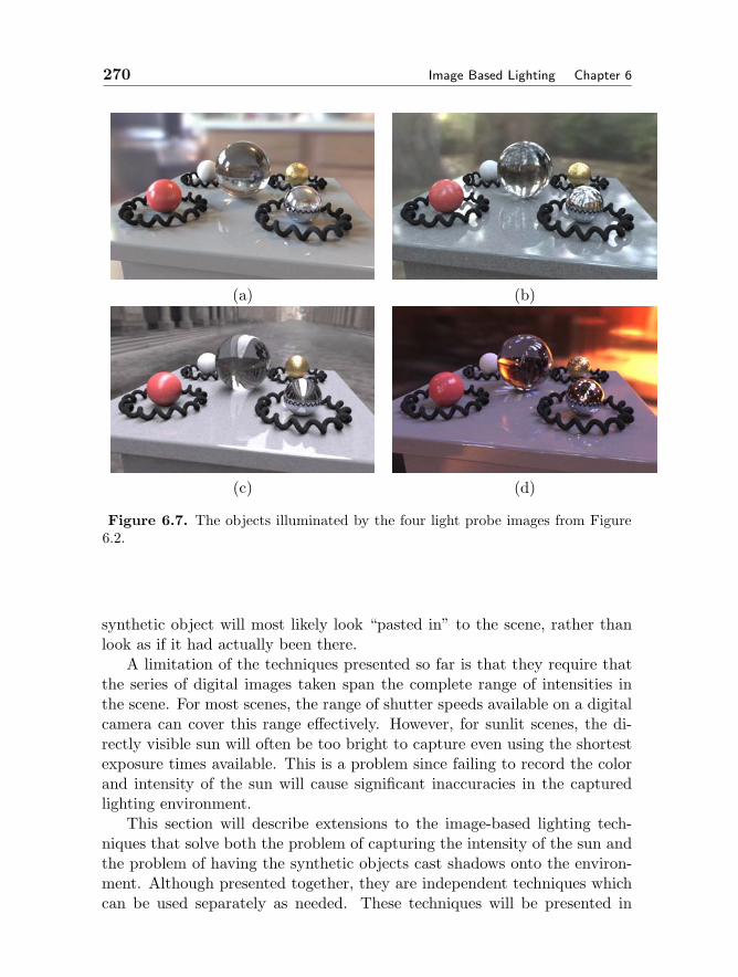
270 Image Based Lighting Chapter 6
(a) (b)
(c) (d)
Figure 6.7. The objects illuminated by the four light probe images from Figure6.2.
synthetic object will most likely look “pasted in” to the scene, rather thanlook as if it had actually been there.
A limitation of the techniques presented so far is that they require thatthe series of digital images taken span the complete range of intensities inthe scene. For most scenes, the range of shutter speeds available on a digitalcamera can cover this range effectively. However, for sunlit scenes, the di-rectly visible sun will often be too bright to capture even using the shortestexposure times available. This is a problem since failing to record the colorand intensity of the sun will cause significant inaccuracies in the capturedlighting environment.
This section will describe extensions to the image-based lighting tech-niques that solve both the problem of capturing the intensity of the sun andthe problem of having the synthetic objects cast shadows onto the environ-ment. Although presented together, they are independent techniques whichcan be used separately as needed. These techniques will be presented in
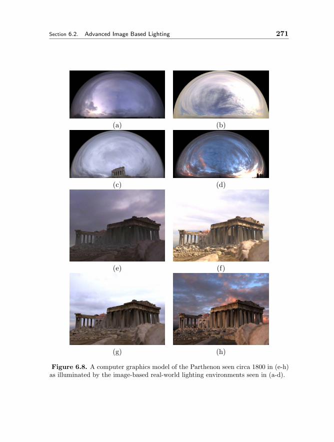
Section 6.2. Advanced Image Based Lighting 271
(a) (b)
(c) (d)
(e) (f)
(g) (h)
Figure 6.8. A computer graphics model of the Parthenon seen circa 1800 in (e-h)as illuminated by the image-based real-world lighting environments seen in (a-d).

272 Image Based Lighting Chapter 6
(a) (b)
Figure 6.9. (a) The Guggenheim Museum in Bilbao. (b) A background plateimage taken in front of the museum.
the form of a new image-based lighting example, also using the RADIANCErendering system.
6.2.1 Capturing a Light Probe in Direct Sunlight
The example we will use is that of placing a new sculpture and some spheresin front of the Guggenheim museum in Bilbao, Spain seen in Fig. 6.9(a). Tocreate this example, I first photographed a background plate image using aCanon EOS-D60 digital camera on a tripod as in Fig. 6.9(b). The image wastaken with a 24mm lens at ASA 100 sensitivity, f/11 aperture, and 1/60thof a second shutter speed. A shadow from a nearby lamp post can be seenbeing cast along the ground.
To capture the lighting, I placed a three-inch mirrored sphere on a secondtripod in front of the camera as in Fig. 6.10. I left the first camera in thesame place, pointing in the same direction, since that would make it easier toalign the probe and background images later. In order to keep the reflectionof the camera small in the sphere, I placed the sphere approximately onemeter away from the camera, and then changed to a 200mm telephoto lensin order for the sphere to appear relatively large in the frame. I used a remoterelease for the camera shutter to avoid moving the camera while capturing thelighting, and I took advantage of the camera’s automatic exposure bracketing(AEB) feature to quickly shoot the mirrored sphere at 1/60th, 1/250th, and1/1000th of a second. These images are shown in Fig. 6.11(a-c). The imageswere recorded using the camera’s “RAW” mode which saves uncompressedimage data to the camera’s memory card. This ensures capturing the bestpossible image quality and for this camera has the desirable effect that theimage pixel values exhibit a linear response to incident light in this mode.
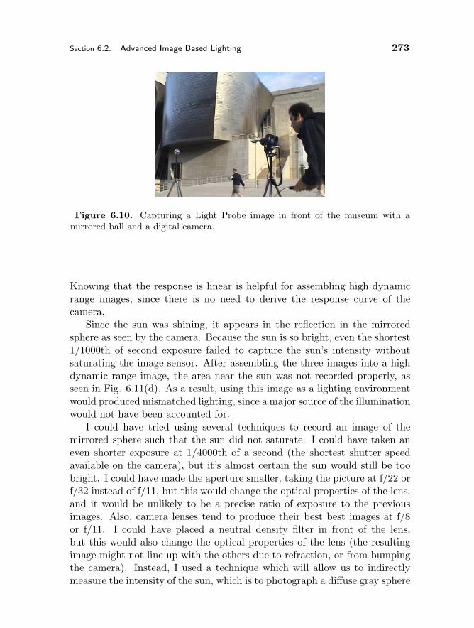
Section 6.2. Advanced Image Based Lighting 273
Figure 6.10. Capturing a Light Probe image in front of the museum with amirrored ball and a digital camera.
Knowing that the response is linear is helpful for assembling high dynamicrange images, since there is no need to derive the response curve of thecamera.
Since the sun was shining, it appears in the reflection in the mirroredsphere as seen by the camera. Because the sun is so bright, even the shortest1/1000th of second exposure failed to capture the sun’s intensity withoutsaturating the image sensor. After assembling the three images into a highdynamic range image, the area near the sun was not recorded properly, asseen in Fig. 6.11(d). As a result, using this image as a lighting environmentwould produced mismatched lighting, since a major source of the illuminationwould not have been accounted for.
I could have tried using several techniques to record an image of themirrored sphere such that the sun did not saturate. I could have taken aneven shorter exposure at 1/4000th of a second (the shortest shutter speedavailable on the camera), but it’s almost certain the sun would still be toobright. I could have made the aperture smaller, taking the picture at f/22 orf/32 instead of f/11, but this would change the optical properties of the lens,and it would be unlikely to be a precise ratio of exposure to the previousimages. Also, camera lenses tend to produce their best best images at f/8or f/11. I could have placed a neutral density filter in front of the lens,but this would also change the optical properties of the lens (the resultingimage might not line up with the others due to refraction, or from bumpingthe camera). Instead, I used a technique which will allow us to indirectlymeasure the intensity of the sun, which is to photograph a diffuse gray sphere

274 Image Based Lighting Chapter 6
(a) (b)
(c) (d)
Figure 6.11. (a-c) A series of images of a mirrored sphere in the Bilbao scenetaken at 1/60th, 1/250th, and 1/1000th of a second. (d) Detail of the sun area of(c), showing the overexposed areas in a dark color.
Figure 6.12. Photographing a diffuse grey sphere to determine the intensity ofthe sun.
in the same location (Fig. 6.12).The image of the diffuse grey sphere will allow us to reconstruct the
intensity of the sun in the following way. Suppose that we had actually
Section 6.2. Advanced Image Based Lighting 275
been able to capture the correct color and intensity of the sun in the lightprobe image. Then, if we were to use that light probe image to illuminatea synthetic diffuse grey sphere, it should have the same appearance as thereal grey sphere actually illuminated by the lighting environment. However,since the light probe failed to record the complete intensity of the sun, therendered diffuse sphere will not match the real diffuse sphere, and in fact wewould expect it to be significantly darker. As we will see, the amount bywhich the rendered sphere is darker in each of the three color channels tellsus the correct color and intensity for the sun.
The first part of this process is to make sure that all of the images thathave been taken are radiometrically consistent. So far, we’ve recorded lightin three different ways: seen directly with the 24mm lens, seen reflected inthe mirrored sphere through the 200mm lens, and finally as reflected off ofthe diffuse sphere with the 200mm lens. Although the 24mm and 200mmlenses were both set to an f/11 aperture, they did not necessarily transmitthe same amount of light to the image sensor. To measure this difference,we can photograph a white spot of light in our laboratory with the camerasto determine the transmission ratio between the two lenses at these twof/stops, as seen in Fig. 6.13. The measurement recorded that the spot inthe 24mm lens image appeared 1.42 times as bright in the red channel, 1.40times as bright in green, and 1.38 times as bright in blue compared to the200mm lens image. Using these results, we can multiply the pixel valuesof the images acquired with the 200mm lens by (1.42, 1.40, 1.38) so that theimages represent places in the scene with equal colors and intensities equally.I could have been even more precise by measuring the relative amount oflight transmitted as a spatially varying function across each lens, perhapsby photographing the spot in different places in the field of view of eachlens. At wider f/stops, many lenses, particularly wide angle ones, transmitsignificantly less light to the corners of the image than to the center. Sincethe f/11 f/stop was reasonably small I made the assumption that these effectswould not be significant.
Continuing toward the goal of radiometric consistency, we should notethat neither the mirrored sphere nor the diffuse sphere are 100% reflective.The diffuse sphere is intentionally painted grey instead of white so that itwill be less likely to saturate the image sensor if an automatic light meter isbeing employed. I measured the paint’s reflectivity by painting a flat surfacewith the same color, and then photographing the surface in diffuse natu-ral illumination. In the scene I also placed a similarly oriented reflectancestandard, a white disk of material specially designed to reflect nearly 100%of all wavelengths of light across the visible spectrum. By dividing the av-
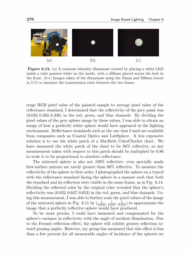
276 Image Based Lighting Chapter 6
(a) (b) (c)
Figure 6.13. (a) A constant intensity illuminant created by placing a white LEDinside a tube painted white on the inside, with a diffuser placed across the hole inthe front. (b-c) Images taken of the illuminant using the 24mm and 200mm lensesat f/11 to measure the transmission ratio between the two lenses.
erage RGB pixel value of the painted sample to average pixel value of thereflectance standard, I determined that the reflectivity of the grey paint was(0.032, 0.333, 0.346) in the red, green, and blue channels. By dividing thepixel values of the grey sphere image by these values, I was able to obtain animage of how a perfectly white sphere would have appeared in the lightingenvironment. Reflectance standards such as the one that I used are availablefrom companies such as Coastal Optics and LabSphere. A less expensivesolution is to use the white patch of a MacBeth ColorChecker chart. Wehave measured the white patch of the chart to be 86% reflective, so anymeasurement taken with respect to this patch should be multiplied by 0.86to scale it to be proportional to absolute reflectance.
The mirrored sphere is also not 100% reflective; even specially madefirst-surface mirrors are rarely greater than 90% reflective. To measure thereflectivity of the sphere to first order, I photographed the sphere on a tripodwith the reflectance standard facing the sphere in a manner such that boththe standard and its reflection were visible in the same frame, as in Fig. 6.14.Dividing the reflected color by the original color revealed that the sphere’sreflectivity was (0.632, 0.647, 0.653) in the red, green, and blue channels. Us-ing this measurement, I was able to further scale the pixel values of the imageof the mirrored sphere in Fig. 6.11 by ( 1
0.632 ,1
0.647 ,1
0.653) to approximate theimage that a perfectly reflective sphere would have produced.
To be more precise, I could have measured and compensated for thesphere’s variance in reflectivity with the angle of incident illumination. Dueto the Fresnel reflection effect, the sphere will exhibit greater reflection to-ward grazing angles. However, my group has measured that this effect is lessthan a few percent for all measurable angles of incidence of the spheres we
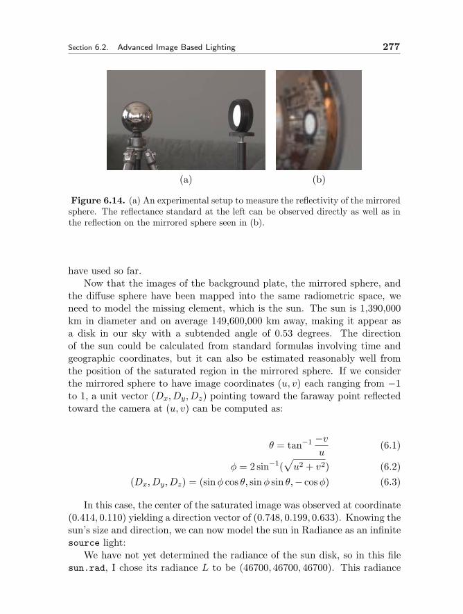
Section 6.2. Advanced Image Based Lighting 277
(a) (b)
Figure 6.14. (a) An experimental setup to measure the reflectivity of the mirroredsphere. The reflectance standard at the left can be observed directly as well as inthe reflection on the mirrored sphere seen in (b).
have used so far.Now that the images of the background plate, the mirrored sphere, and
the diffuse sphere have been mapped into the same radiometric space, weneed to model the missing element, which is the sun. The sun is 1,390,000km in diameter and on average 149,600,000 km away, making it appear asa disk in our sky with a subtended angle of 0.53 degrees. The directionof the sun could be calculated from standard formulas involving time andgeographic coordinates, but it can also be estimated reasonably well fromthe position of the saturated region in the mirrored sphere. If we considerthe mirrored sphere to have image coordinates (u, v) each ranging from −1to 1, a unit vector (Dx, Dy, Dz) pointing toward the faraway point reflectedtoward the camera at (u, v) can be computed as:
θ = tan−1 −vu
(6.1)
φ = 2 sin−1(√u2 + v2) (6.2)
(Dx, Dy, Dz) = (sinφ cos θ, sinφ sin θ,− cosφ) (6.3)
In this case, the center of the saturated image was observed at coordinate(0.414, 0.110) yielding a direction vector of (0.748, 0.199, 0.633). Knowing thesun’s size and direction, we can now model the sun in Radiance as an infinitesource light:
We have not yet determined the radiance of the sun disk, so in this filesun.rad, I chose its radiance L to be (46700, 46700, 46700). This radiance
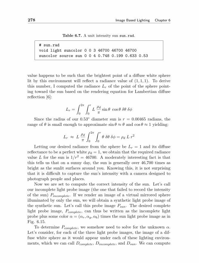
278 Image Based Lighting Chapter 6
Table 6.7. A unit intensity sun sun.rad.
# sun.radvoid light suncolor 0 0 3 46700 46700 46700suncolor source sun 0 0 4 0.748 0.199 0.633 0.53
value happens to be such that the brightest point of a diffuse white spherelit by this environment will reflect a radiance value of (1, 1, 1). To derivethis number, I computed the radiance Lr of the point of the sphere point-ing toward the sun based on the rendering equation for Lambertian diffusereflection [6]:
Lr =∫ 2π
0
∫ r
0Lρdπ
sin θ cos θ δθ δφ
Since the radius of our 0.53 diameter sun is r = 0.00465 radians, therange of θ is small enough to approximate sin θ ≈ θ and cos θ ≈ 1 yielding:
Lr ≈ Lρdπ
∫ 2π
0
∫ r
0θ δθ δφ = ρd L r
2
Letting our desired radiance from the sphere be Lr = 1 and its diffusereflectance to be a perfect white ρd = 1, we obtain that the required radiancevalue L for the sun is 1/r2 = 46700. A moderately interesting fact is thatthis tells us that on a sunny day, the sun is generally over 46,700 times asbright as the sunlit surfaces around you. Knowing this, it is not surprisingthat it is difficult to capture the sun’s intensity with a camera designed tophotograph people and places.
Now we are set to compute the correct intensity of the sun. Let’s callour incomplete light probe image (the one that failed to record the intensityof the sun) Pincomplete. If we render an image of a virtual mirrored sphereilluminated by only the sun, we will obtain a synthetic light probe image ofthe synthetic sun. Let’s call this probe image Psun. The desired completelight probe image, Pcomplete, can thus be written as the incomplete lightprobe plus some color α = (αr, αg, αb) times the sun light probe image as inFig. 6.15.
To determine Pcomplete, we somehow need to solve for the unknown α.Let’s consider, for each of the three light probe images, the image of a dif-fuse white sphere as it would appear under each of these lighting environ-ments, which we can call Dcomplete, Dincomplete, and Dsun. We can compute
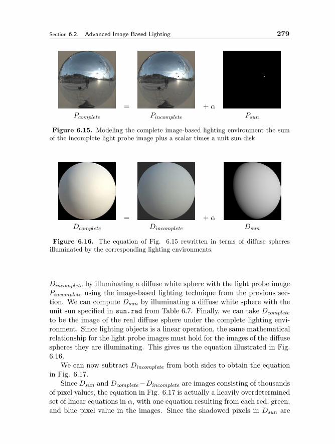
Section 6.2. Advanced Image Based Lighting 279
= + αPcomplete Pincomplete Psun
Figure 6.15. Modeling the complete image-based lighting environment the sumof the incomplete light probe image plus a scalar times a unit sun disk.
= + αDcomplete Dincomplete Dsun
Figure 6.16. The equation of Fig. 6.15 rewritten in terms of diffuse spheresilluminated by the corresponding lighting environments.
Dincomplete by illuminating a diffuse white sphere with the light probe imagePincomplete using the image-based lighting technique from the previous sec-tion. We can compute Dsun by illuminating a diffuse white sphere with theunit sun specified in sun.rad from Table 6.7. Finally, we can take Dcomplete
to be the image of the real diffuse sphere under the complete lighting envi-ronment. Since lighting objects is a linear operation, the same mathematicalrelationship for the light probe images must hold for the images of the diffusespheres they are illuminating. This gives us the equation illustrated in Fig.6.16.
We can now subtract Dincomplete from both sides to obtain the equationin Fig. 6.17.
Since Dsun and Dcomplete−Dincomplete are images consisting of thousandsof pixel values, the equation in Fig. 6.17 is actually a heavily overdeterminedset of linear equations in α, with one equation resulting from each red, green,and blue pixel value in the images. Since the shadowed pixels in Dsun are
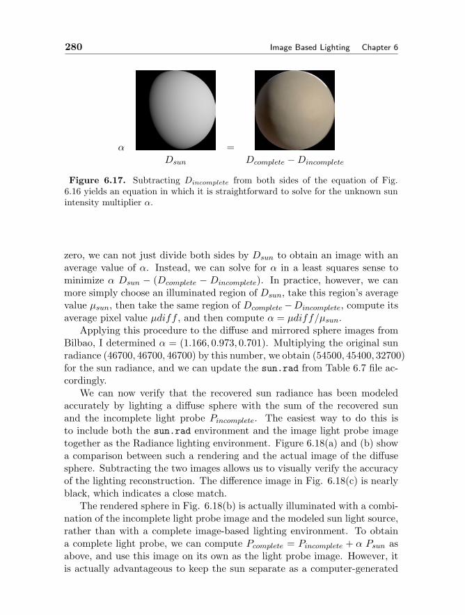
280 Image Based Lighting Chapter 6
α =Dsun Dcomplete −Dincomplete
Figure 6.17. Subtracting Dincomplete from both sides of the equation of Fig.6.16 yields an equation in which it is straightforward to solve for the unknown sunintensity multiplier α.
zero, we can not just divide both sides by Dsun to obtain an image with anaverage value of α. Instead, we can solve for α in a least squares sense tominimize α Dsun − (Dcomplete − Dincomplete). In practice, however, we canmore simply choose an illuminated region of Dsun, take this region’s averagevalue µsun, then take the same region of Dcomplete−Dincomplete, compute itsaverage pixel value µdiff , and then compute α = µdiff/µsun.
Applying this procedure to the diffuse and mirrored sphere images fromBilbao, I determined α = (1.166, 0.973, 0.701). Multiplying the original sunradiance (46700, 46700, 46700) by this number, we obtain (54500, 45400, 32700)for the sun radiance, and we can update the sun.rad from Table 6.7 file ac-cordingly.
We can now verify that the recovered sun radiance has been modeledaccurately by lighting a diffuse sphere with the sum of the recovered sunand the incomplete light probe Pincomplete. The easiest way to do this isto include both the sun.rad environment and the image light probe imagetogether as the Radiance lighting environment. Figure 6.18(a) and (b) showa comparison between such a rendering and the actual image of the diffusesphere. Subtracting the two images allows us to visually verify the accuracyof the lighting reconstruction. The difference image in Fig. 6.18(c) is nearlyblack, which indicates a close match.
The rendered sphere in Fig. 6.18(b) is actually illuminated with a combi-nation of the incomplete light probe image and the modeled sun light source,rather than with a complete image-based lighting environment. To obtaina complete light probe, we can compute Pcomplete = Pincomplete + α Psun asabove, and use this image on its own as the light probe image. However, itis actually advantageous to keep the sun separate as a computer-generated
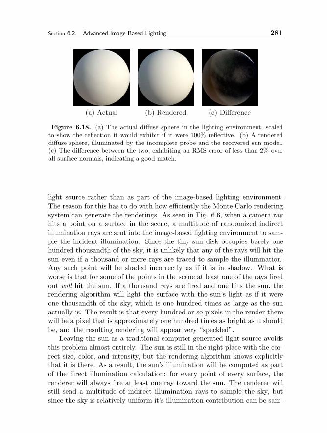
Section 6.2. Advanced Image Based Lighting 281
(a) Actual (b) Rendered (c) Difference
Figure 6.18. (a) The actual diffuse sphere in the lighting environment, scaledto show the reflection it would exhibit if it were 100% reflective. (b) A rendereddiffuse sphere, illuminated by the incomplete probe and the recovered sun model.(c) The difference between the two, exhibiting an RMS error of less than 2% overall surface normals, indicating a good match.
light source rather than as part of the image-based lighting environment.The reason for this has to do with how efficiently the Monte Carlo renderingsystem can generate the renderings. As seen in Fig. 6.6, when a camera rayhits a point on a surface in the scene, a multitude of randomized indirectillumination rays are sent into the image-based lighting environment to sam-ple the incident illumination. Since the tiny sun disk occupies barely onehundred thousandth of the sky, it is unlikely that any of the rays will hit thesun even if a thousand or more rays are traced to sample the illumination.Any such point will be shaded incorrectly as if it is in shadow. What isworse is that for some of the points in the scene at least one of the rays firedout will hit the sun. If a thousand rays are fired and one hits the sun, therendering algorithm will light the surface with the sun’s light as if it wereone thousandth of the sky, which is one hundred times as large as the sunactually is. The result is that every hundred or so pixels in the render therewill be a pixel that is approximately one hundred times as bright as it shouldbe, and the resulting rendering will appear very “speckled”.
Leaving the sun as a traditional computer-generated light source avoidsthis problem almost entirely. The sun is still in the right place with the cor-rect size, color, and intensity, but the rendering algorithm knows explicitlythat it is there. As a result, the sun’s illumination will be computed as partof the direct illumination calculation: for every point of every surface, therenderer will always fire at least one ray toward the sun. The renderer willstill send a multitude of indirect illumination rays to sample the sky, butsince the sky is relatively uniform it’s illumination contribution can be sam-

282 Image Based Lighting Chapter 6
pled sufficiently accurately with a few hundred rays. (If any of the indirectillumination rays do hit the sun, they will not add to the illumination of thepixel, since the sun’s contribution is already being considered in the directcalculation.) The result is that renderings with low noise can be computedwith a small fraction of the rays which would otherwise be necessary if thesun were represented as part of the image-based lighting environment.
The technique of representing a concentrated image-based area of illumi-nation as a traditional CG light sources can be extended to multiple lightsources within more complex lighting environments. Section 6.2.3 describeshow the windows and ceiling lamps within St. Peter’s Basilica were modeledas local area lights to efficiently render the animation Fiat Lux. Techniqueshave also been developed to approximate image-based lighting environmentsentirely as clusters of traditional point light sources [5, 17, 2]. These al-gorithms let the user specify the desired number of light sources and thenuse clustering algorithms to choose the light source positions and intensitiesto best approximate the lighting environment. Such techniques can makeit possible to simulate image-based lighting effects using more traditionalrendering systems.
At this point we have successfully recorded a light probe in a scene wherethe sun is directly visible; in the next section we will use this recordedillumination to realistically place some new objects in front of the museum.
6.2.2 Compositing objects into the scene including shadows
The next step of rendering the synthetic objects into the scene involves recon-structing the scene’s viewpoint and geometry, rather than its illumination.We first need to obtain a good estimate of the position, orientation, andfocal length of the camera at the time that it photographed the backgroundplate image. Then, we will also need to create a basic 3D model of the scenethat includes the surfaces with which the new objects will photometricallyinteract – in our case, this is the ground plane upon which the objects willsit.
Determining the camera pose and local scene geometry could be donethrough manual survey at the time of the shoot or through trial and errorafterwards. For architectural scenes such as ours, it is usually possible to ob-tain these measurements through photogrammetry, often from just the onebackground photograph. Fig. 6.19 shows the use of the Facade photogram-metric modeling system described in [12] to reconstruct the camera pose andthe local scene geometry based on a set of user-marked edge features in thescene.
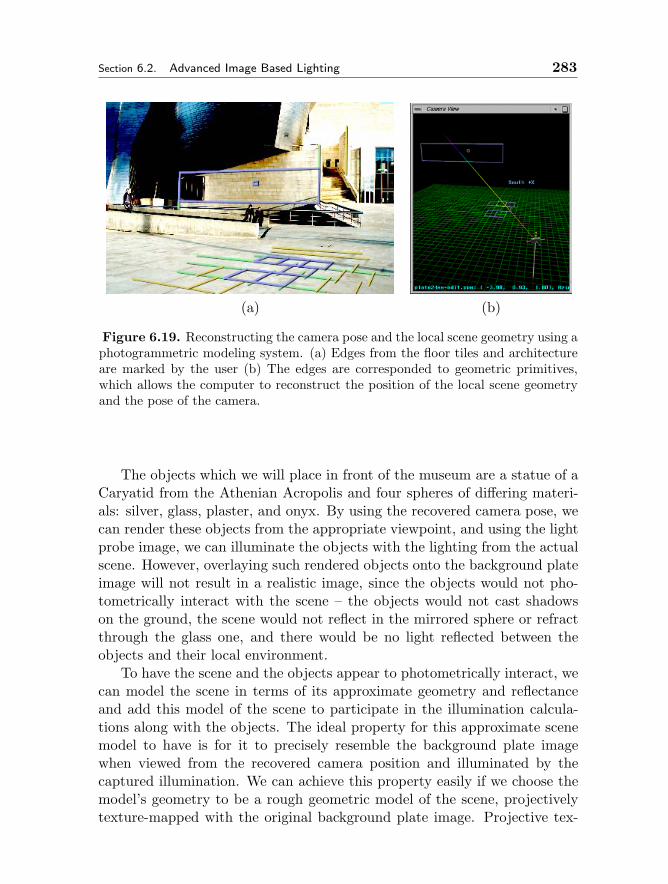
Section 6.2. Advanced Image Based Lighting 283
(a) (b)
Figure 6.19. Reconstructing the camera pose and the local scene geometry using aphotogrammetric modeling system. (a) Edges from the floor tiles and architectureare marked by the user (b) The edges are corresponded to geometric primitives,which allows the computer to reconstruct the position of the local scene geometryand the pose of the camera.
The objects which we will place in front of the museum are a statue of aCaryatid from the Athenian Acropolis and four spheres of differing materi-als: silver, glass, plaster, and onyx. By using the recovered camera pose, wecan render these objects from the appropriate viewpoint, and using the lightprobe image, we can illuminate the objects with the lighting from the actualscene. However, overlaying such rendered objects onto the background plateimage will not result in a realistic image, since the objects would not pho-tometrically interact with the scene – the objects would not cast shadowson the ground, the scene would not reflect in the mirrored sphere or refractthrough the glass one, and there would be no light reflected between theobjects and their local environment.
To have the scene and the objects appear to photometrically interact, wecan model the scene in terms of its approximate geometry and reflectanceand add this model of the scene to participate in the illumination calcula-tions along with the objects. The ideal property for this approximate scenemodel to have is for it to precisely resemble the background plate imagewhen viewed from the recovered camera position and illuminated by thecaptured illumination. We can achieve this property easily if we choose themodel’s geometry to be a rough geometric model of the scene, projectivelytexture-mapped with the original background plate image. Projective tex-

284 Image Based Lighting Chapter 6
ture mapping is the image-based rendering process of assigning surface colorsas if the image were being projected onto the scene as if from a virtual slideprojector placed at the original camera position. Since we have recoveredthe camera position, performing this mapping is a straightforward process inmany rendering systems. A useful property of projective texture mapping isthat when an image is projected onto geometry, a rendering of the scene willlook just like the original image when viewed from the same viewpoint as theprojection. When viewed from different viewpoints, the similarity betweenthe rendered viewpoint the original scene will be a function of how far thecamera has moved and the accuracy of the scene geometry. Fig. 6.20 showsa bird’s-eye view of the background plate projected onto a horizontal poly-gon for the ground plane and a vertical polygon representing the museum inthe distance; the positions of these two polygons were determined from thephotogrammetric modeling step in Fig. 6.19.
When a texture map is applied to a surface, the renderer can be toldto treat the texture map’s pixel values either as measures of the surface’sradiance, or as measures of the surface’s reflectance. If we choose to map thevalues on as radiance, then the surface will be treated as an emissive surfacethat appears precisely the same no matter how it is illuminated or what sortof objects are placed in its vicinity. This is in fact how we have been mappingthe light probe images onto the sky dome as the “glow” material to becomeimage-based lighting environments. However, for the ground beneath theobjects, this is not the behavior we want. We instead need to texture-mapthe ground plane with reflectance values, which will allow the ground plane toparticipate in the same illumination computation as the added objects, thusallowing the ground plane to receive shadows and interreflect light with theobjects. In Radiance, we can do this by specifying the material as “plastic”with no specular component and then modulating the diffuse color values ofthe surface using the projective texture map.
The problem we now face is that the pixels of the background plate imageare actually measurements of radiance – the amount light reflecting from thescene toward the camera – rather than reflectance, which is what we needto project onto the local scene. Reflectance values represent the proportionof incident light that a surface reflects back (also known as the material’salbedo), and range from zero (0% of the light is reflected) to one (100% ofthe light is reflected). Considered in RGB for the three color channels, thesereflectance values represent what we traditionally think of as the inherent“color” of a surface, since they are independent of the incident illumination.Radiance values are different in that they can range from zero to arbitrarilyhigh values. Thus, it is generally inaccurate to use radiance values as if they

Section 6.2. Advanced Image Based Lighting 285
Figure 6.20. The final scene, seen from above instead of from the original cameraviewpoint. The background plate is mapped onto the local scene ground planeand a billboard for the museum behind. The light probe image is mapped onto theremainder of the ground plane, the billboard, and the sky. The synthetic objects areset on top of the local scene and both the local scene and the objects are illuminatedby the captured lighting environment.
were reflectance values.As it turns out, we can convert the radiance values from the background
plate image into reflectance values using the following relationship:
radiance = irradiance× reflectanceor
reflectance = radiance / irradiance
Since the background plate image tells us the radiance for each point onthe local scene, all we need to know is the irradiance of each point as well.As it turns out, these irradiance values can be determined using the illumi-nation which we recorded within the environment in the following manner.We assign the local scene surfaces a diffuse material property of known re-flectance, for example 50% grey, or (0.5, 0.5, 0.5) in RGB. We then renderthis local scene as illuminated by the image-based lighting environment tocompute the appearance of the scene under the lighting, seen in Fig. 6.21(a).
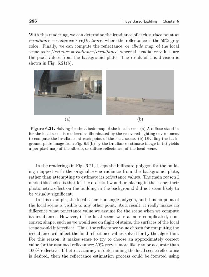
286 Image Based Lighting Chapter 6
With this rendering, we can determine the irradiance of each surface point atirradiance = radiance / reflectance, where the reflectance is the 50% greycolor. Finally, we can compute the reflectance, or albedo map, of the localscene as reflectance = radiance/irradiance, where the radiance values arethe pixel values from the background plate. The result of this division isshown in Fig. 6.21(b).
(a) (b)
Figure 6.21. Solving for the albedo map of the local scene. (a) A diffuse stand-infor the local scene is rendered as illuminated by the recovered lighting environmentto compute the irradiance at each point of the local scene. (b) Dividing the back-ground plate image from Fig. 6.9(b) by the irradiance estimate image in (a) yieldsa per-pixel map of the albedo, or diffuse reflectance, of the local scene.
In the renderings in Fig. 6.21, I kept the billboard polygon for the build-ing mapped with the original scene radiance from the background plate,rather than attempting to estimate its reflectance values. The main reason Imade this choice is that for the objects I would be placing in the scene, theirphotometric effect on the building in the background did not seem likely tobe visually significant.
In this example, the local scene is a single polygon, and thus no point ofthe local scene is visible to any other point. As a result, it really makes nodifference what reflectance value we assume for the scene when we computeits irradiance. However, if the local scene were a more complicated, non-convex shape, such as we would see on flight of stairs, the surfaces of the localscene would interreflect. Thus, the reflectance value chosen for computing theirrradiance will affect the final reflectance values solved for by the algorithm.For this reason, it makes sense to try to choose an approximately correctvalue for the assumed reflectance; 50% grey is more likely to be accurate than100% reflective. If better accuracy in determining the local scene reflectanceis desired, then the reflectance estimation process could be iterated using
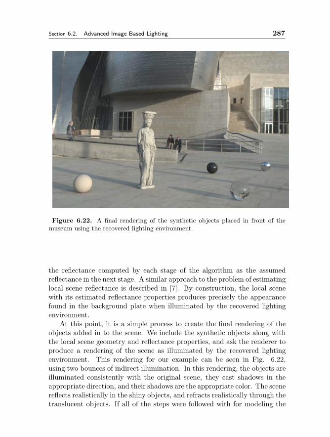
Section 6.2. Advanced Image Based Lighting 287
Figure 6.22. A final rendering of the synthetic objects placed in front of themuseum using the recovered lighting environment.
the reflectance computed by each stage of the algorithm as the assumedreflectance in the next stage. A similar approach to the problem of estimatinglocal scene reflectance is described in [7]. By construction, the local scenewith its estimated reflectance properties produces precisely the appearancefound in the background plate when illuminated by the recovered lightingenvironment.
At this point, it is a simple process to create the final rendering of theobjects added in to the scene. We include the synthetic objects along withthe local scene geometry and reflectance properties, and ask the renderer toproduce a rendering of the scene as illuminated by the recovered lightingenvironment. This rendering for our example can be seen in Fig. 6.22,using two bounces of indirect illumination. In this rendering, the objects areilluminated consistently with the original scene, they cast shadows in theappropriate direction, and their shadows are the appropriate color. The scenereflects realistically in the shiny objects, and refracts realistically through thetranslucent objects. If all of the steps were followed with for modeling the
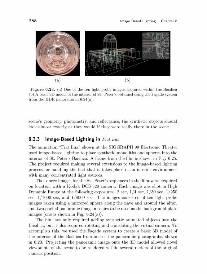
288 Image Based Lighting Chapter 6
(a) (b)
Figure 6.23. (a) One of the ten light probe images acquired within the Basilica(b) A basic 3D model of the interior of St. Peter’s obtained using the Facade systemfrom the HDR panorama in 6.24(a).
scene’s geometry, photometry, and reflectance, the synthetic objects shouldlook almost exactly as they would if they were really there in the scene.
6.2.3 Image-Based Lighting in Fiat Lux
The animation “Fiat Lux” shown at the SIGGRAPH 99 Electronic Theaterused image-based lighting to place synthetic monoliths and spheres into theinterior of St. Peter’s Basilica. A frame from the film is shown in Fig. 6.25.The project required making several extensions to the image-based lightingprocess for handling the fact that it takes place in an interior environmentwith many concentrated light sources.
The source images for the St. Peter’s sequences in the film were acquiredon location with a Kodak DCS-520 camera. Each image was shot in HighDynamic Range at the following exposures: 2 sec, 1/4 sec, 1/30 sec, 1/250sec, 1/1000 sec, and 1/8000 sec. The images consisted of ten light probeimages taken using a mirrored sphere along the nave and around the altar,and two partial panoramic image mosaics to be used as the background plateimages (one is shown in Fig. 6.24(a)).
The film not only required adding synthetic animated objects into theBasilica, but it also required rotating and translating the virtual camera. Toaccomplish this, we used the Facade system to create a basic 3D model ofthe interior of the Basilica from one of the panoramic photographs, shownin 6.23. Projecting the panoramic image onto the 3D model allowed novelviewpoints of the scene to be rendered within several meters of the originalcamera position.
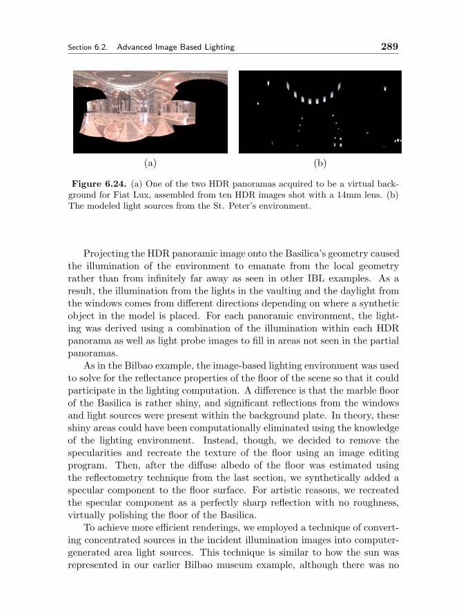
Section 6.2. Advanced Image Based Lighting 289
(a) (b)
Figure 6.24. (a) One of the two HDR panoramas acquired to be a virtual back-ground for Fiat Lux, assembled from ten HDR images shot with a 14mm lens. (b)The modeled light sources from the St. Peter’s environment.
Projecting the HDR panoramic image onto the Basilica’s geometry causedthe illumination of the environment to emanate from the local geometryrather than from infinitely far away as seen in other IBL examples. As aresult, the illumination from the lights in the vaulting and the daylight fromthe windows comes from different directions depending on where a syntheticobject in the model is placed. For each panoramic environment, the light-ing was derived using a combination of the illumination within each HDRpanorama as well as light probe images to fill in areas not seen in the partialpanoramas.
As in the Bilbao example, the image-based lighting environment was usedto solve for the reflectance properties of the floor of the scene so that it couldparticipate in the lighting computation. A difference is that the marble floorof the Basilica is rather shiny, and significant reflections from the windowsand light sources were present within the background plate. In theory, theseshiny areas could have been computationally eliminated using the knowledgeof the lighting environment. Instead, though, we decided to remove thespecularities and recreate the texture of the floor using an image editingprogram. Then, after the diffuse albedo of the floor was estimated usingthe reflectometry technique from the last section, we synthetically added aspecular component to the floor surface. For artistic reasons, we recreatedthe specular component as a perfectly sharp reflection with no roughness,virtually polishing the floor of the Basilica.
To achieve more efficient renderings, we employed a technique of convert-ing concentrated sources in the incident illumination images into computer-generated area light sources. This technique is similar to how the sun wasrepresented in our earlier Bilbao museum example, although there was no
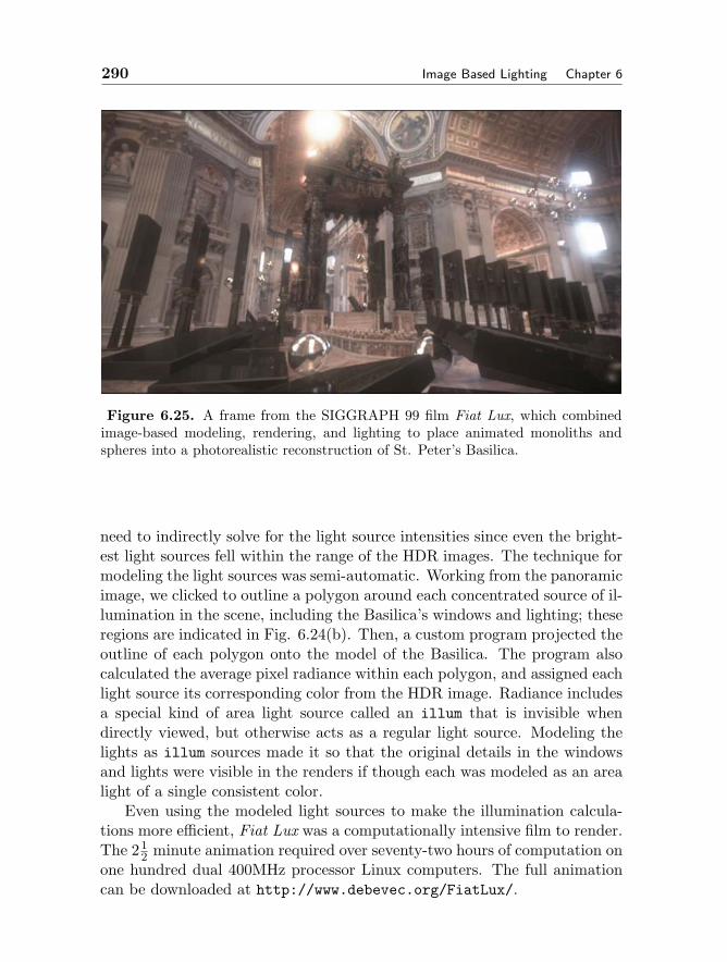
290 Image Based Lighting Chapter 6
Figure 6.25. A frame from the SIGGRAPH 99 film Fiat Lux, which combinedimage-based modeling, rendering, and lighting to place animated monoliths andspheres into a photorealistic reconstruction of St. Peter’s Basilica.
need to indirectly solve for the light source intensities since even the bright-est light sources fell within the range of the HDR images. The technique formodeling the light sources was semi-automatic. Working from the panoramicimage, we clicked to outline a polygon around each concentrated source of il-lumination in the scene, including the Basilica’s windows and lighting; theseregions are indicated in Fig. 6.24(b). Then, a custom program projected theoutline of each polygon onto the model of the Basilica. The program alsocalculated the average pixel radiance within each polygon, and assigned eachlight source its corresponding color from the HDR image. Radiance includesa special kind of area light source called an illum that is invisible whendirectly viewed, but otherwise acts as a regular light source. Modeling thelights as illum sources made it so that the original details in the windowsand lights were visible in the renders if though each was modeled as an arealight of a single consistent color.
Even using the modeled light sources to make the illumination calcula-tions more efficient, Fiat Lux was a computationally intensive film to render.The 21
2 minute animation required over seventy-two hours of computation onone hundred dual 400MHz processor Linux computers. The full animationcan be downloaded at http://www.debevec.org/FiatLux/.

Section 6.2. Advanced Image Based Lighting 291
6.2.4 Capturing and Rendering Spatially-Varying Illumination
The techniques presented so far capture light at discrete points in space astwo-dimensional omnidirectional image datasets. In reality, light changesthroughout space, and this changing illumination can be described as thefive-dimensional plenoptic function [1]. This function is essentially a collec-tion of light probe images (θ, φ) taken at every possible (x, y, z) point inspace. The most dramatic changes in lighting occur at shadow boundaries,where a light source may be visible in one light probe image and occludedin a neighboring one. More often, changes in light within space are moregradual, consisting of changes resulting from moving closer to and furtherfrom sources of direct and indirect illumination.
Two recent papers [19, 13] have shown that the plenoptic function canbe reduced to a four-dimensional function for free regions of space. Sincelight travels in straight lines and maintains its radiance along a ray, any rayrecorded passing through a plane Π can be used to extrapolate the plenopticfunction to any other point along that ray. These papers then showed thatthe appearance of a scene, recorded as a 2D array of 2D images taken from aplanar grid of points in space, could be used to synthesize views of the scenefrom viewpoints both in front of and behind the plane.
A key observation in image-based lighting is that there is no fundamen-tal difference between capturing images of a scene and capturing images ofillumination. It is illumination that is being captured in both cases, and oneneeds only pay attention to having sufficient dynamic range and linear sensorresponse when using cameras to capture light. It thus stands to reason thatthe light field capture technique would provide a method of capturing andreconstructing varying illumination within a volume of space.
To this end, our group has constructed two different devices for capturingincident light fields [28]. The first, shown in Fig. 6.26(a) is a straightforwardextrapolation of the mirrored ball capture technique, consisting of a 12 ×12 array of 1-inch mirrored spheres fixed to a board. Although the adjacentspheres reflect each other near the horizon, the array captures images witha nearly 160 unoccluded field of view. A single HDR image of the spheresprovides a four-dimensional dataset of wide field-of-view images sampledacross a planar surface. However, since each sphere occupied just a smallpart of the image, the angular resolution of the device was limited, andthe 12 × 12 array of spheres provided even poorer sampling in the spatialdimensions.
To improve the resolution, we built a second device for capturing inci-dent light fields (ILFs) consisting of a video camera with a 185 fisheye lens
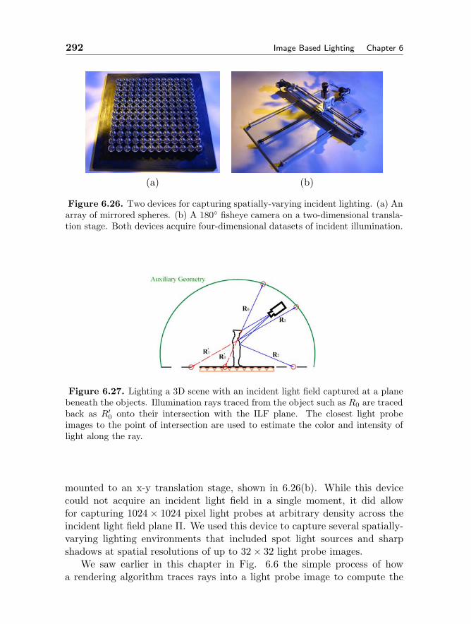
292 Image Based Lighting Chapter 6
(a) (b)
Figure 6.26. Two devices for capturing spatially-varying incident lighting. (a) Anarray of mirrored spheres. (b) A 180 fisheye camera on a two-dimensional transla-tion stage. Both devices acquire four-dimensional datasets of incident illumination.
Figure 6.27. Lighting a 3D scene with an incident light field captured at a planebeneath the objects. Illumination rays traced from the object such as R0 are tracedback as R′
0 onto their intersection with the ILF plane. The closest light probeimages to the point of intersection are used to estimate the color and intensity oflight along the ray.
mounted to an x-y translation stage, shown in 6.26(b). While this devicecould not acquire an incident light field in a single moment, it did allowfor capturing 1024 × 1024 pixel light probes at arbitrary density across theincident light field plane Π. We used this device to capture several spatially-varying lighting environments that included spot light sources and sharpshadows at spatial resolutions of up to 32× 32 light probe images.
We saw earlier in this chapter in Fig. 6.6 the simple process of howa rendering algorithm traces rays into a light probe image to compute the
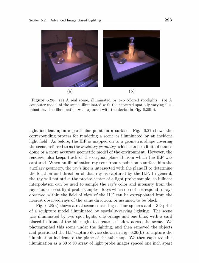
Section 6.2. Advanced Image Based Lighting 293
(a) (b)
Figure 6.28. (a) A real scene, illuminated by two colored spotlights. (b) Acomputer model of the scene, illuminated with the captured spatially-varying illu-mination. The illumination was captured with the device in Fig. 6.26(b).
light incident upon a particular point on a surface. Fig. 6.27 shows thecorresponding process for rendering a scene as illuminated by an incidentlight field. As before, the ILF is mapped on to a geometric shape coveringthe scene, referred to as the auxiliary geometry, which can be a finite-distancedome or a more accurate geometric model of the environment. However, therenderer also keeps track of the original plane Π from which the ILF wascaptured. When an illumination ray sent from a point on a surface hits theauxilary geometry, the ray’s line is intersected with the plane Π to determinethe location and direction of that ray as captured by the ILF. In general,the ray will not strike the precise center of a light probe sample, so bilinearinterpolation can be used to sample the ray’s color and intensity from theray’s four closest light probe samples. Rays which do not correspond to raysobserved within the field of view of the ILF can be extrapolated from thenearest observed rays of the same direction, or assumed to be black.
Fig. 6.28(a) shows a real scene consisting of four spheres and a 3D printof a sculpture model illuminated by spatially-varying lighting. The scenewas illuminated by two spot lights, one orange and one blue, with a cardplaced in front of the blue light to create a shadow across the scene. Wephotographed this scene under the lighting, and then removed the objectsand positioned the ILF capture device shown in Fig. 6.26(b) to capture theillumination incident to the plane of the table top. We then captured thisillumination as a 30× 30 array of light probe images spaced one inch apart
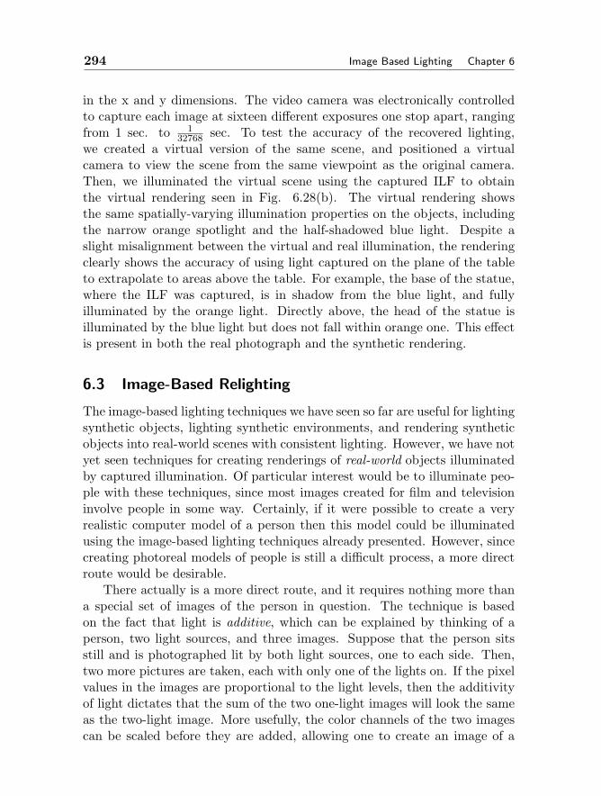
294 Image Based Lighting Chapter 6
in the x and y dimensions. The video camera was electronically controlledto capture each image at sixteen different exposures one stop apart, rangingfrom 1 sec. to 1
32768 sec. To test the accuracy of the recovered lighting,we created a virtual version of the same scene, and positioned a virtualcamera to view the scene from the same viewpoint as the original camera.Then, we illuminated the virtual scene using the captured ILF to obtainthe virtual rendering seen in Fig. 6.28(b). The virtual rendering showsthe same spatially-varying illumination properties on the objects, includingthe narrow orange spotlight and the half-shadowed blue light. Despite aslight misalignment between the virtual and real illumination, the renderingclearly shows the accuracy of using light captured on the plane of the tableto extrapolate to areas above the table. For example, the base of the statue,where the ILF was captured, is in shadow from the blue light, and fullyilluminated by the orange light. Directly above, the head of the statue isilluminated by the blue light but does not fall within orange one. This effectis present in both the real photograph and the synthetic rendering.
6.3 Image-Based Relighting
The image-based lighting techniques we have seen so far are useful for lightingsynthetic objects, lighting synthetic environments, and rendering syntheticobjects into real-world scenes with consistent lighting. However, we have notyet seen techniques for creating renderings of real-world objects illuminatedby captured illumination. Of particular interest would be to illuminate peo-ple with these techniques, since most images created for film and televisioninvolve people in some way. Certainly, if it were possible to create a veryrealistic computer model of a person then this model could be illuminatedusing the image-based lighting techniques already presented. However, sincecreating photoreal models of people is still a difficult process, a more directroute would be desirable.
There actually is a more direct route, and it requires nothing more thana special set of images of the person in question. The technique is basedon the fact that light is additive, which can be explained by thinking of aperson, two light sources, and three images. Suppose that the person sitsstill and is photographed lit by both light sources, one to each side. Then,two more pictures are taken, each with only one of the lights on. If the pixelvalues in the images are proportional to the light levels, then the additivityof light dictates that the sum of the two one-light images will look the sameas the two-light image. More usefully, the color channels of the two imagescan be scaled before they are added, allowing one to create an image of a
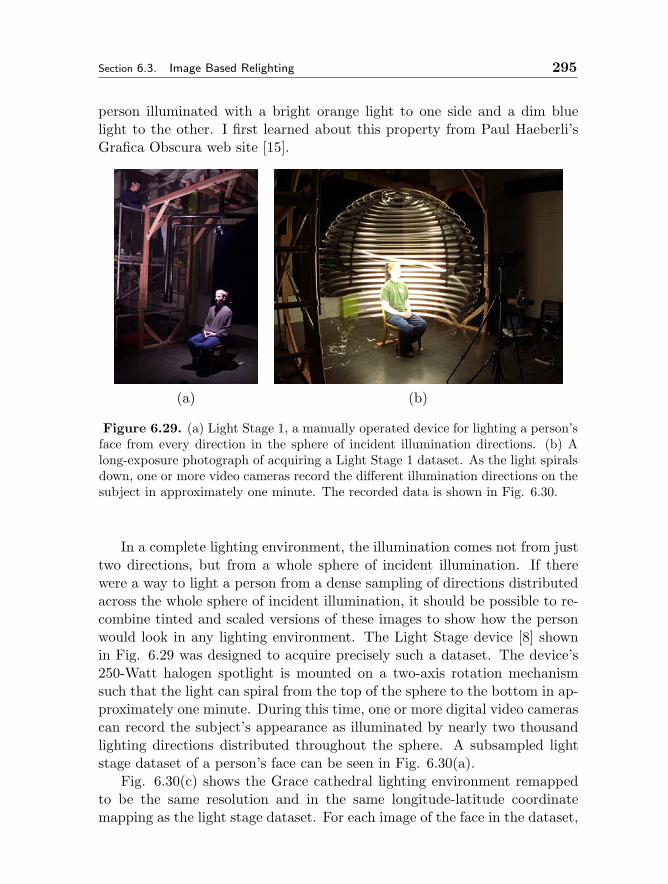
Section 6.3. Image Based Relighting 295
person illuminated with a bright orange light to one side and a dim bluelight to the other. I first learned about this property from Paul Haeberli’sGrafica Obscura web site [15].
(a) (b)
Figure 6.29. (a) Light Stage 1, a manually operated device for lighting a person’sface from every direction in the sphere of incident illumination directions. (b) Along-exposure photograph of acquiring a Light Stage 1 dataset. As the light spiralsdown, one or more video cameras record the different illumination directions on thesubject in approximately one minute. The recorded data is shown in Fig. 6.30.
In a complete lighting environment, the illumination comes not from justtwo directions, but from a whole sphere of incident illumination. If therewere a way to light a person from a dense sampling of directions distributedacross the whole sphere of incident illumination, it should be possible to re-combine tinted and scaled versions of these images to show how the personwould look in any lighting environment. The Light Stage device [8] shownin Fig. 6.29 was designed to acquire precisely such a dataset. The device’s250-Watt halogen spotlight is mounted on a two-axis rotation mechanismsuch that the light can spiral from the top of the sphere to the bottom in ap-proximately one minute. During this time, one or more digital video camerascan record the subject’s appearance as illuminated by nearly two thousandlighting directions distributed throughout the sphere. A subsampled lightstage dataset of a person’s face can be seen in Fig. 6.30(a).
Fig. 6.30(c) shows the Grace cathedral lighting environment remappedto be the same resolution and in the same longitude-latitude coordinatemapping as the light stage dataset. For each image of the face in the dataset,
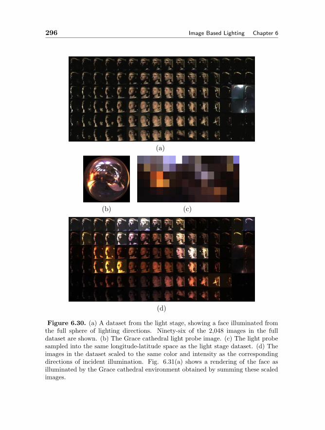
296 Image Based Lighting Chapter 6
(a)
(b) (c)
(d)
Figure 6.30. (a) A dataset from the light stage, showing a face illuminated fromthe full sphere of lighting directions. Ninety-six of the 2,048 images in the fulldataset are shown. (b) The Grace cathedral light probe image. (c) The light probesampled into the same longitude-latitude space as the light stage dataset. (d) Theimages in the dataset scaled to the same color and intensity as the correspondingdirections of incident illumination. Fig. 6.31(a) shows a rendering of the face asilluminated by the Grace cathedral environment obtained by summing these scaledimages.

Section 6.3. Image Based Relighting 297
(a) (b) (c) (d)
Figure 6.31. Renderings of the light stage dataset from Fig. 6.30 as illuminatedby four image-based lighting environments. (a) Grace Cathedral. (b) EucalyptusGrove. (c) Uffizi Gallery. (d) St. Peter’s Basilica.
the resampled light probe indicates the color and intensity of the light fromthe environment in the corresponding direction. Thus, we can multiply thered, green, and blue color channels of each light stage image by the amountof red, green, and blue light in the corresponding direction in the lightingenvironment to obtain the modulated dataset that appears in Fig. 6.30(d).Fig. 6.31(a) shows the result of summing all of the scaled images in Fig.6.30(d), producing an image of the subject as they would appear illuminatedby the light of Grace Cathedral. Results obtained for three more lightingenvironments are shown in Fig. 6.31(b-d).
The process of computing the weighted sum of the face images is simplecomputation, but it requires accessing hundreds of megabytes of data for eachrendering. The process can be accelerated by performing the computationon compressed versions of the original images. In particular, if the imagesare compressed using an orthonormal transform such as the Discrete CosineTransform, the linear combination of the images can be computed directlyfrom the basis coefficients of the original images as shown in [25]. The FaceDemo program written by Chris Tchou and Dan Maas (Fig. 6.32) uses DCT-compressed versions of the face datasets to allow interactive face relightingwith either light probe images or user-controlled light sources in real time.More recent work has used Spherical Harmonics [24, 23] and Wavelets [22]to perform real-time image-based lighting on virtual light stage datasets of
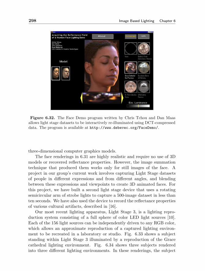
298 Image Based Lighting Chapter 6
Figure 6.32. The Face Demo program written by Chris Tchou and Dan Maasallows light stage datasets to be interactively re-illuminated using DCT-compresseddata. The program is available at http://www.debevec.org/FaceDemo/.
three-dimensional computer graphics models.The face renderings in 6.31 are highly realistic and require no use of 3D
models or recovered reflectance properties. However, the image summationtechnique that produced them works only for still images of the face. Aproject in our group’s current work involves capturing Light Stage datasetsof people in different expressions and from different angles, and blendingbetween these expressions and viewpoints to create 3D animated faces. Forthis project, we have built a second light stage device that uses a rotatingsemicircular arm of strobe lights to capture a 500-image dataset in less thanten seconds. We have also used the device to record the reflectance propertiesof various cultural artifacts, described in [16].
Our most recent lighting apparatus, Light Stage 3, is a lighting repro-duction system consisting of a full sphere of color LED light sources [10].Each of the 156 light sources can be independently driven to any RGB color,which allows an approximate reproduction of a captured lighting environ-ment to be recreated in a laboratory or studio. Fig. 6.33 shows a subjectstanding within Light Stage 3 illuminated by a reproduction of the Gracecathedral lighting environment. Fig. 6.34 shows three subjects renderedinto three different lighting environments. In these renderings, the subject
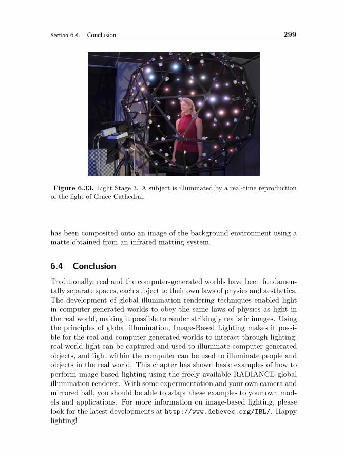
Section 6.4. Conclusion 299
Figure 6.33. Light Stage 3. A subject is illuminated by a real-time reproductionof the light of Grace Cathedral.
has been composited onto an image of the background environment using amatte obtained from an infrared matting system.
6.4 Conclusion
Traditionally, real and the computer-generated worlds have been fundamen-tally separate spaces, each subject to their own laws of physics and aesthetics.The development of global illumination rendering techniques enabled lightin computer-generated worlds to obey the same laws of physics as light inthe real world, making it possible to render strikingly realistic images. Usingthe principles of global illumination, Image-Based Lighting makes it possi-ble for the real and computer generated worlds to interact through lighting:real world light can be captured and used to illuminate computer-generatedobjects, and light within the computer can be used to illuminate people andobjects in the real world. This chapter has shown basic examples of how toperform image-based lighting using the freely available RADIANCE globalillumination renderer. With some experimentation and your own camera andmirrored ball, you should be able to adapt these examples to your own mod-els and applications. For more information on image-based lighting, pleaselook for the latest developments at http://www.debevec.org/IBL/. Happylighting!
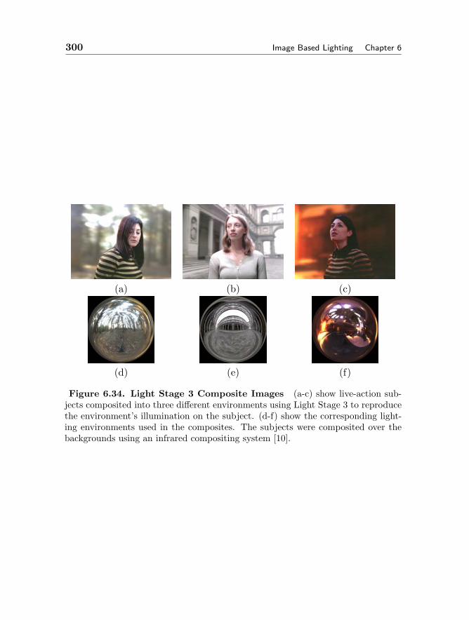
300 Image Based Lighting Chapter 6
(a) (b) (c)
(d) (e) (f)
Figure 6.34. Light Stage 3 Composite Images (a-c) show live-action sub-jects composited into three different environments using Light Stage 3 to reproducethe environment’s illumination on the subject. (d-f) show the corresponding light-ing environments used in the composites. The subjects were composited over thebackgrounds using an infrared compositing system [10].
Bibliography 301
Acknowledgements
The work described in this chapter represents the work of many individuals.Greg Ward wrote the RADIANCE rendering system and provided advice forusing it optimally in an image-based lighting context. Marcos Fajardo wrotethe Arnold renderer and provided helpful HDR and IBL support. ChristineWaggoner and Son Chang helped carry out early light source identificationidentification experiments. Andreas Wenger wrote the Canon RAW to HDRconverter and Chris Tchou wrote the HDR Shop image editing programused to process the Bilbao images. Maya Martinez helped compose theBilbao scene. Teddy Kim provided light probe assistance in Bilbao. TimHawkins helped acquire the HDR images used in Fiat Lux and helped lead theFiat Lux team including Westley Sarokin, H.P. Duiker, Tal Garfinkel, JennyHuang, and Christine Cheng. The work presented here owes its support tothe National Science Foundation, the California MICRO program, IntervalResearch Corporation, the Digital Media Innovation Program, InteractivePictures Corporation, U.S. Army contract #DAAD19-99-D-0046, TOPPANPrinting Co. Ltd., and the University of Southern California Office of theProvost.
Editors’ note: The color version of the figures in this chapter can be foundin the accompanying DVD.
Bibliography
[1] E. H. Adelson and J. R. Bergen. Computational Models of Visual Processing,chapter 1. MIT Press, Cambridge, Mass., 1991. The Plenoptic Function andthe Elements of Early Vision.
[2] S. Agarwal, R. Ramamoorthi, S. Belongie, and H. W. Jensen. Structuredimportance sampling of environment maps. ACM Transactions on Graphics,22(3):605–612, July 2003.
[3] J. F. Blinn. Texture and reflection in computer generated images. Communi-cations of the ACM, 19(10):542–547, October 1976.
[4] S. E. Chen. Quicktime vr - an image-based approach to virtual environmentnavigation. In Proceedings of SIGGRAPH 95, Computer Graphics Proceedings,Annual Conference Series, pages 29–38, Aug. 1995.
[5] J. Cohen and P. Debevec. The LightGen HDRShop Plugin. Available atwww.debevec.org/HDRShop/, 2001.
[6] M. F. Cohen and J. R. Wallace. Radiosity and Realistic Image Synthesis, chap-ter 2, page 32. Academic Press, 1993.
[7] P. Debevec. Rendering synthetic objects into real scenes: Bridging traditionaland image-based graphics with global illumination and high dynamic rangephotography. In SIGGRAPH 98, July 1998.

302 Image Based Lighting Chapter 6
[8] P. Debevec, T. Hawkins, C. Tchou, H.-P. Duiker, W. Sarokin, and M. Sagar.Acquiring the reflectance field of a human face. Proceedings of SIGGRAPH2000, pages 145–156, July 2000.
[9] P. Debevec and D. Lemmon. Image based lighting. In SIGGRAPH 2001 Notesfor Course 14, August 2001.
[10] P. Debevec, A. Wenger, C. Tchou, A. Gardner, J. Waese, and T. Hawkins. Alighting reproduction approach to live-action compositing. ACM Transactionson Graphics, 21(3):547–556, July 2002.
[11] P. E. Debevec and J. Malik. Recovering high dynamic range radiance mapsfrom photographs. In SIGGRAPH 97, pages 369–378, August 1997.
[12] P. E. Debevec, C. J. Taylor, and J. Malik. Modeling and rendering architec-ture from photographs: A hybrid geometry- and image-based approach. InSIGGRAPH 96, pages 11–20, August 1996.
[13] S. J. Gortler, R. Grzeszczuk, R. Szeliski, and M. F. Cohen. The Lumigraph. InSIGGRAPH 96, pages 43–54, 1996.
[14] N. Greene. Environment mapping and other application of world projections.IEEE Computer Graphics and Applications, 6(11):21–29, November 1986.
[15] P. Haeberli. Synthetic lighting for photography. Available athttp://www.sgi.com/grafica/synth/index.html, January 1992.
[16] T. Hawkins, J. Cohen, and P. Debevec. A photometric approach to digitizingcultural artifacts. In Proc. 2nd International Symposium on Virtual Reality,Archaeology, and Cultural Heritage (VAST 2001), pages 333–342, December2001.
[17] T. Kollig and A. Keller. Efficient illumination by high dynamic range images.In Eurographics Symposium on Rendering: 14th Eurographics Workshop onRendering, pages 45–51, June 2003.
[18] G. W. Larson. Overcoming gamut and dynamic range limitations in digitalimages. In Proceedings of the Sixth Color Imaging Conference, November 1998.
[19] M. Levoy and P. Hanrahan. Light field rendering. In SIGGRAPH 96, pages31–42, 1996.
[20] G. S. Miller and C. R. Hoffman. Illumination and reflection maps: Simulatedobjects in simulated and real environments. In SIGGRAPH 84 Course Notesfor Advanced Computer Graphics Animation, July 1984.
[21] T. Mitsunaga and S. K. Nayar. Radiometric self calibration. In Proc. IEEEConf. on Computer Vision and Pattern Recognition, Fort Collins, June 1999.
[22] R. Ng, R. Ramamoorthi, and P. Hanrahan. All-frequency shadows usingnon-linear wavelet lighting approximation. ACM Transactions on Graphics,22(3):376–381, July 2003.
[23] R. Ramamoorthi and P. Hanrahan. Frequency space environment map render-ing. ACM Transactions on Graphics, 21(3):517–526, July 2002.
[24] P.-P. Sloan, J. Kautz, and J. Snyder. Precomputed radiance transfer for real-time rendering in dynamic, low-frequency lighting environments. ACM Trans-actions on Graphics, 21(3):527–536, July 2002.
[25] B. Smith and L. Rowe. Compressed domain processing of JPEG-encoded im-ages. Real-Time Imaging, 2(2):3–17, 1996.

Bibliography 303
[26] R. Szeliski and H.-Y. Shum. Creating full view panoramic mosaics and environ-ment maps. In Proceedings of SIGGRAPH 97, Computer Graphics Proceedings,Annual Conference Series, pages 251–258, Aug. 1997.
[27] C. Tchou and P. Debevec. HDR Shop. Available athttp://www.debevec.org/HDRShop, 2001.
[28] J. Unger, A. Wenger, T. Hawkins, A. Gardner, and P. Debevec. Capturing andrendering with incident light fields. In Eurographics Symposium on Rendering:14th Eurographics Workshop on Rendering, June 2003.
[29] G. Ward. Real pixels. Graphics Gems II, pages 80–83, 1991.

Chapter 7
COMPUTER VISION INVISUAL EFFECTS
Doug Roble
7.1 Introduction
Computer vision has changed the way movies are made. Sure, computergraphics gets all the press, but computer vision techniques have made sig-nificant impact on the way films with visual effects are envisioned, planned,and executed. This chapter will examine the state of the practice of com-puter vision techniques in visual effects. We will also examine the changescomputer vision has brought to the industry, the new capabilities directorsand visual effects creators have available and what is desired in the future.
Let us examine the concept of visual effects in terms of computer vision.The main task of visual effects is to manipulate or add things to an im-age. Artists are very skilled, but the more information they have about theoriginal image or the more tools the computer presents to them, the moreeffective they can be.
Computer vision has made a huge impact in the field of visual effectsover the last decade. In the early 1990s we saw the shift away from usingphysical models and photographic techniques to create and add fantasticthings to an image. It has became commonplace to scan each frame offilm into the computer and composite computer generated elements with thefilmed background image. Digitizing the filmed image is so common nowthat whole films are digitized, manipulated in the digital realm and filmedout to a negative for printing. (“Oh Brother, Where Art Thou?” is a goodexample of this. The color of each frame of the film was digitally adjusted
305

306 Computer Vision in Visual Effects Chapter 7
to give the film its “look”.) And, of course, digital cameras are starting tomake in-roads into Hollywood. “Star Wars, Attack of the Clones” was shotcompletely with a digital camera.
Once a sequence of frames is digitized, it becomes possible to apply stan-dard computer vision algorithms to the digitized sequence in order to extractas much information as possible from the image. Structure from motion, fea-ture tracking, and optical flow are just some of the techniques that we willexamine in relation to film making.
7.2 Computer Vision Problems Unique to Film
7.2.1 Welcome to the Set
A film set is a unique work environment. It is a place of high creativity,incredible tension, sometimes numbing boredom. The set is a place of conflictin the creation of art. The producers and their staff are responsible forkeeping the show on budget and on time and they fear and respect the set,for filming on a set is very expensive indeed. The director and crew aretrying to get the best possible images and performances on film. These twoforces are at odds with each other on the set and often the computer visionpeople are caught in the middle!
The set is where it all begins for the digital artists responsible for whatwe call “data integration”. Data integration is acquiring, analyzing, andmanaging all the data recorded from the set. It is common for a visual effectsfacility to send a team of one or more people to the set with the standardcrew. Before, during, and after filming, the data integration crew pop in andout of the set, recording everything they can about the makeup of the set.This is where the trouble starts: the producers are not crazy about the dataintegration crew, they are an added expense for a not so obvious result. Thedirectors can get irritated with the data integration team because it is justone more disturbance on the set, slowing them down from getting one moretake before the light fades or the producers start glaring again.
At least that is the way it was in the beginning. Movie makers are gettingmuch more savvy and accustomed to the power that computer vision providesthem in the film making process. While a director might be slightly annoyedthat a vision person is slowing the process slightly, he or she is infinitelymore annoyed when the visual effects supervisor tells him how to film ascene because of the inability of the effects people to deal with a kind ofcamera move.
Watch some movies from the 1980s. Special effects were booming and
Section 7.2. Computer Vision Problems Unique to Film 307
there were elaborate, effects-laden movies in that decade. But effects shotsalways telegraphed themselves to the audience because the camera stoppedmoving! If a stop motion creature effect or some elaborate set extension wasplanned, the director could either lock the camera down or move it in verylimited ways (a rotation about the lens’ nodal axis or a simple zoom couldusually be handled, but nothing more). Now directors can film however theywant. The camera can be on giant crane, a plane, a Steadicam, or evena hand held shot. If there is not enough information in the scene for thecomputer vision algorithms to work, we drop objects in the scene and paintthem out later! (A couple of problem scenes for the ambitious researcher outthere: a camera mounted in a plane flying over the ocean on a clear day -computing the camera location each frame is tricky, all your reference pointsare moving! And yet, if the camera track is not correct, inserting a boaton the surface of the ocean will look wrong. Or a camera carried by a skierfilming on a smooth glacier - this is where adding objects make the problemgo away, but without them, there is no hope!)
For a major production with many effects shots a team of 2 to 3 peopleare sent to the set to record information. They typically stay with the filmcrew throughout the production, traveling to outdoors locations and workingon the indoors sets that have been constructed. This data integration crewrecords everything they can to make the digital artists’ lives easier. Here isa list of things that the crew tries to capture:
– Environment Maps: Environment maps are spherical (or semi-spherical)photographs of the set, generally taken from near center of the set ornear where the digital object is going to be inserted into the set. Dig-ital artists began running into the center of a sets with a chrome ballin the late 80s and early 90s. The quickest, cheapest way to acquirean environment map is to go to your garden supply center, buy a dec-orative chrome ball and mount it on a tripod. Then, when the chancepresents itself, run into the center of the set, and snap two quick pho-tographs of the chrome ball from both sides. It is relatively easy tomap the pixels of the image to the area on the ball and from that, itis possible to project the images onto a spherical environment map.
This environment map is then used in the renderer to render the digitalobjects as if they are in the environment of the set. Shiny objectsreflect portions of the set and even diffuse objects change their colordepending on the incident light from the environment maps.
This ability to light digital objects with the light that existed on the sethas caused a flurry of development over the last decade. Paul Debevec
308 Computer Vision in Visual Effects Chapter 7
was a pioneer in the use of High Dynamic Range imagery, used inconjunction with environment maps, showing just how powerful thecombination can be.
A snapshot of a chrome ball is only so useful. It creates a picture of a360 degree environment, but since film (be it digital or photochemical)has a limited dynamic range, much of the information in the imageis inaccurate. All photographers have experienced this to one extent.Setting the exposure controls to capture detail in the dark areas ofa scene mean that the bright areas will be over exposed and clipped.Alternately, setting the exposure for accurately capturing the brightareas of the scene mean that the dark areas will have no informationin them.
The concept behind high dynamic range photography is simple; takemultiple images of a scene each with a different exposure. Then, com-bine the images into one image by using only the non-clipped pixelsof the images and an appropriate mapping function. The results areamazing. Instead of an image with 8 bit pixels and values that go from0 to 256, high dynamic range images store floating point numbers thatgo from zero to a very large number indeed. It is even possible (andsometimes very useful) to have negative color values!
There are many advantages to high dynamic range images, but in thecontext of environment maps, the main advantage is that they are anaccurate way of capturing the light energy of the environment, not justa simple snapshot. These environment maps can be used as elaboratelights in a rendering package and can be used to create stunninglyconvincing images. A good introduction to these concepts can be foundin [11] and [3].
– Camera and Object Motion: Computing camera location and mo-tion is where computer vision first made in-roads into the film industry.Directors acknowledged, but did not like, the constraint that the cam-era had to stop moving or move in a very specific way if an effect wasgoing to work.
The first method used to record camera motion did not rely on visualeffects at all. Encoding devices were attached to the moving partsof a crane or a dolly. The measurements from the encoding deviceswere sent to a computer and, combined with an exact knowledge ofthe rig’s geometry, the location and orientation of the camera could bedetermined.
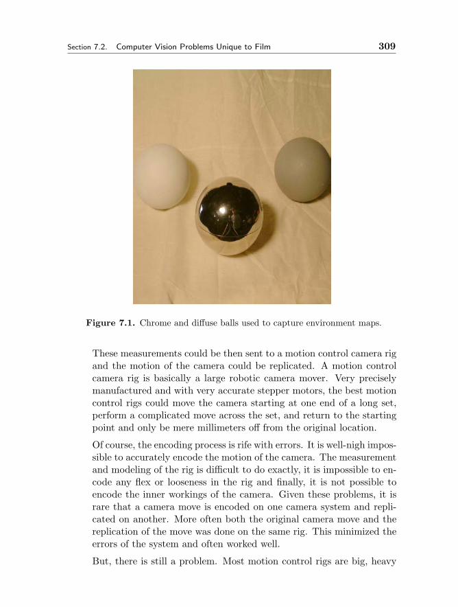
Section 7.2. Computer Vision Problems Unique to Film 309
Figure 7.1. Chrome and diffuse balls used to capture environment maps.
These measurements could be then sent to a motion control camera rigand the motion of the camera could be replicated. A motion controlcamera rig is basically a large robotic camera mover. Very preciselymanufactured and with very accurate stepper motors, the best motioncontrol rigs could move the camera starting at one end of a long set,perform a complicated move across the set, and return to the startingpoint and only be mere millimeters off from the original location.
Of course, the encoding process is rife with errors. It is well-nigh impos-sible to accurately encode the motion of the camera. The measurementand modeling of the rig is difficult to do exactly, it is impossible to en-code any flex or looseness in the rig and finally, it is not possible toencode the inner workings of the camera. Given these problems, it israre that a camera move is encoded on one camera system and repli-cated on another. More often both the original camera move and thereplication of the move was done on the same rig. This minimized theerrors of the system and often worked well.
But, there is still a problem. Most motion control rigs are big, heavy

310 Computer Vision in Visual Effects Chapter 7
machines. They have to be, given the weight of the camera they arecarrying and the need for stiffness in the rig. So they could never movevery quickly. Certainly not as quickly as a hand held camera or usinga dolly or a crane.
Given all these limitations, motion control rigs were only used for shotswith models or very limited shots with actors.
Recently, “real-time” motion control rigs have been used on sets. TheBulldog Motion Control Camera rig from ImageG received a TechnicalAcademy Award in 2001. It is extremely fast and can be used toreproduce very fast camera moves.
What does this all have to do with computer vision? Quite a bit,actually. Motion control rigs are still used in visual effects because itis often much more cost effective to build a detailed model of a ship orlocation rather than constructing it all as a digital set. Industrial Lightand Magic built a large model of a pirate ship and sailed it in a pondbehind their facility for a large number of shots in the film “Pirates ofthe Caribbean (2003)”. It was just more cost effective.
There are two problems associated with motion control rigs and com-puter vision. The first problem is relatively easy. If a model is filmedwith motion control, the images are often enhanced with digital effects.Unfortunately, even though the camera path is known from the motioncontrol move, it cannot be trusted. The path is very repeatable, butit is not sub-pixel accurate in the digital realm - the internal cameramotion and flex of the devices is not recorded. However, the camerapose estimation is a very easy subset of the general problem. Oncefeatures in the image are identified, the motion of the features is easyto predict because of the known motion of the camera. In fact, whilethe overall path of the camera may have errors, the incremental motionfrom one frame to the next is quite accurate. So the camera motion isused to predict the feature motion and a quick template match in thelocal area is performed to find the features to sub-pixel accuracy. Stan-dard structure from motion techniques are used to refine the motion.Convergence is very fast since the starting path is quite good.
The second problem with motion control cameras is quite difficult and,to some extent, impossible to solve. Often it is required to replicate themotion of a handheld camera with the motion control rig. Often a di-rector will film the actors with a “wild” camera in front of a bluescreen.Then, at a later date, the camera move is reproduced on a motion con-
Section 7.2. Computer Vision Problems Unique to Film 311
trol rig filming an elaborate model. The actors are composited withthe filmed model for the final shot. Tracking the camera on the stageis not terribly difficult. The data integration team will place markersor known geometry on the blue screen and pose estimation techniquescan be used to recover the camera path. The problem comes whentransferring the camera motion to the motion control rig.
Motion control rigs do not stop before a frame of film is shot. It isa common misconception, but they do not move, stop, shoot, move,stop... Rather, they shoot the sequence of frames in one continuousmotion. There are many advantages to this but the two overridingbenefits are speed of shooting and motion blur. Stopping before eachframe slows down the motion control rig terribly and stage time isexpensive. If the camera is moving while the shutter is open, onegets motion blur for free. Model shots look very unconvincing withoutmotion blur.
This continuous motion of the rig leads to the problem. Because of thesize of the motion control rig, there are physical limits to the torque ofthe stepper motors and how fast they can move the rig. Therefore, atthe speed that is needed for the shot, the camera may not be able toexactly reproduce the desired motion. When the foreground and back-ground are merged they will not line up and high frequency motionsof the camera move will not be preserved in the background plate.
This problem is difficult to fix. If the problem is extreme enough,the motion control camera motion is tracked (using methods describedabove) and compared with the original camera motion. 3D pointsin the scene are the then projected onto the image plane of the realcamera and the motion control rig. The discrepancy of these pointsis then used to build a general warping field that is applied to thebackground images. Naturally, this is a 2D fix to what is a 3D problemand it is unable to correct all the problems, but it usually suffices. Ofcourse, a generalized warp will filter the image and effectively reducethe resolution of the background image so the images are typicallydigitized at a higher resolution.
– Set and Object Geometry: The data integration team is responsi-ble for capturing geometric information about the set. This can rangefrom some simple measurements of the height of a locked off cameraor where a light is in relation to the camera to full three dimensionalreconstruction of the set with textures and BRDF analysis of the sur-
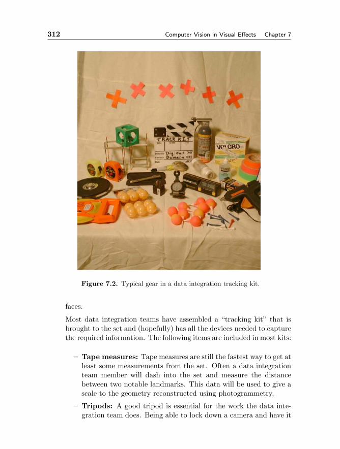
312 Computer Vision in Visual Effects Chapter 7
Figure 7.2. Typical gear in a data integration tracking kit.
faces.
Most data integration teams have assembled a “tracking kit” that isbrought to the set and (hopefully) has all the devices needed to capturethe required information. The following items are included in most kits:
– Tape measures: Tape measures are still the fastest way to get atleast some measurements from the set. Often a data integrationteam member will dash into the set and measure the distancebetween two notable landmarks. This data will be used to give ascale to the geometry reconstructed using photogrammetry.
– Tripods: A good tripod is essential for the work the data inte-gration team does. Being able to lock down a camera and have it
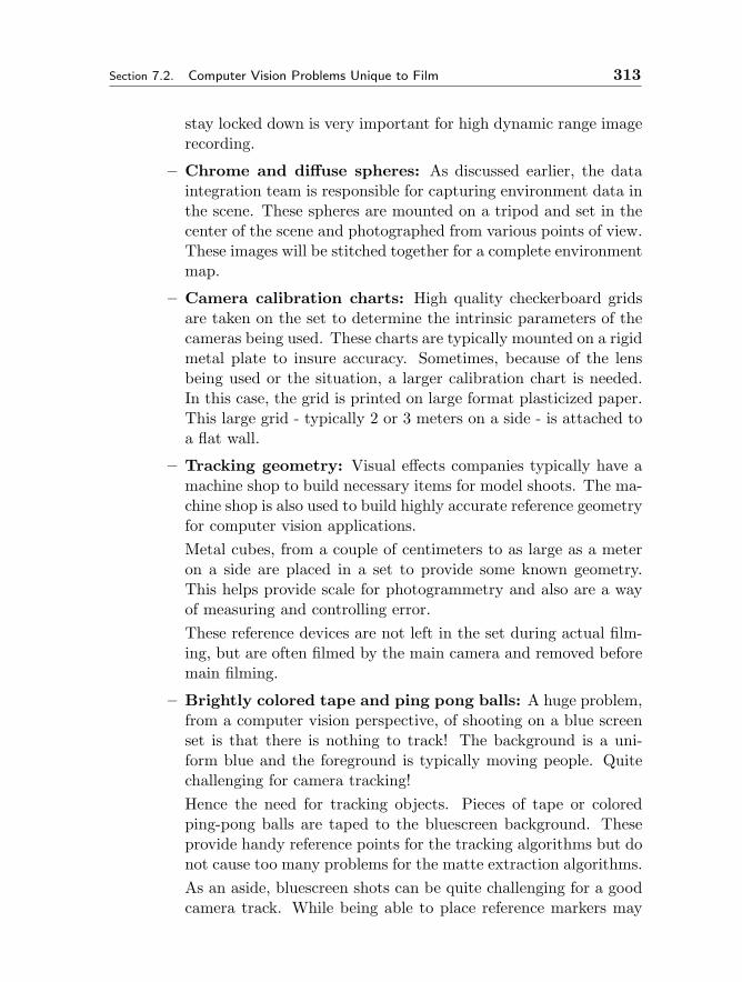
Section 7.2. Computer Vision Problems Unique to Film 313
stay locked down is very important for high dynamic range imagerecording.
– Chrome and diffuse spheres: As discussed earlier, the dataintegration team is responsible for capturing environment data inthe scene. These spheres are mounted on a tripod and set in thecenter of the scene and photographed from various points of view.These images will be stitched together for a complete environmentmap.
– Camera calibration charts: High quality checkerboard gridsare taken on the set to determine the intrinsic parameters of thecameras being used. These charts are typically mounted on a rigidmetal plate to insure accuracy. Sometimes, because of the lensbeing used or the situation, a larger calibration chart is needed.In this case, the grid is printed on large format plasticized paper.This large grid - typically 2 or 3 meters on a side - is attached toa flat wall.
– Tracking geometry: Visual effects companies typically have amachine shop to build necessary items for model shoots. The ma-chine shop is also used to build highly accurate reference geometryfor computer vision applications.Metal cubes, from a couple of centimeters to as large as a meteron a side are placed in a set to provide some known geometry.This helps provide scale for photogrammetry and also are a wayof measuring and controlling error.These reference devices are not left in the set during actual film-ing, but are often filmed by the main camera and removed beforemain filming.
– Brightly colored tape and ping pong balls: A huge problem,from a computer vision perspective, of shooting on a blue screenset is that there is nothing to track! The background is a uni-form blue and the foreground is typically moving people. Quitechallenging for camera tracking!Hence the need for tracking objects. Pieces of tape or coloredping-pong balls are taped to the bluescreen background. Theseprovide handy reference points for the tracking algorithms but donot cause too many problems for the matte extraction algorithms.As an aside, bluescreen shots can be quite challenging for a goodcamera track. While being able to place reference markers may

314 Computer Vision in Visual Effects Chapter 7
Figure 7.3. Large, rigid geometry used for photogrammetry and camera calibra-tion.
seem ideal, there is a delicate balance between placing enoughreference points and too many for an easy matte extraction. (Thereason that the crew was filming in front of a blue screen was tomake it easy!) But often more of a problem is that the blue screenis usually quite a distance away from the actors and is typicallya flat screen. Computing the pose of a camera with points thatare all co-planar can be difficult some times and the fact that thereference points are far away from a camera that probably doesnot move all that much makes accuracy even more challenging.Finally, the actors are always a factor. Depending on the numberof actors, all the tracking markers may be obscured.What happens in the worst case: the camera is moving but theactors have obscured all the reference points? We rely on thedata integration artist to solve the problem by hand. Camerapositions can be interpolated from known points, but in worstcase sections, there is no alternative to solving it using the artist’sskill at knowing “what looks good”.
– A total station survey device: Back in the early 1990s, whencomputer vision techniques were starting to make an impact onfilming and the set, it was quite common to hire survey crew

Section 7.2. Computer Vision Problems Unique to Film 315
to create a survey of reference points on the set. These pointswere used in a camera pose estimation algorithm to compute thelocation of a moving camera for each frame of film.
As computer vision techniques became commonplace, visual ef-fects studios purchased their own survey devices and trained peo-ple in their use. Now, almost every studio owns a “total station”.“Total station” is the generic name for the survey devices usedby burly government workers... often seen blocking traffic. A to-tal station is a tripod mounted, highly accurate, laser distanceand angle measure. A total station has an accurate telescopingsight and a laser pointer. Once the station is set up, the surveyperson simply sights or points the laser at a spot in the terrainand presses a button. The distance to the spot is measured usingphase measurement. The angle and distance provide the 3D lo-cation of the point. Key points in the set can be digitized quitequickly.
The problem with total stations is that they are time consumingto set up. And if one moves the station, there is a realignmentprocess to compute the location of the total station in relationto the first setup point. Also, the only points that are digitizedare the points that are selected during the session. If the dataintegration artist needs to compute a point that the person on thetotal station did not compute, different photogrammetry basedtechniques need to be used.
The huge advantage of a total station is that a high accurate ref-erence geometry of key points in the set is built. This can beenormously helpful for camera or object tracking later. Relyingsolely on structure from motion techniques to compute the loca-tion of the camera is unwise - those techniques are notoriously badif the camera focal length changes during the shot. This will cer-tainly happen during a zoom and often happens during a simplechange of focus. With reference geometry the camera’s intrinsicparameters can be calculated from frame to frame. This gives thedirector the ultimate freedom on a set.
– Digital cameras with different kinds of lenses includinga fisheye: Of course, the data integration team carries a digi-tal camera on the set. This is used to record the layout of theset, reconstruct the geometry of the set and build environmentmaps. The cameras are usually high resolution and have cali-
316 Computer Vision in Visual Effects Chapter 7
brated lenses.Data integration teams usually carry a high quality fisheye lens tomake environment maps, but there are issues with these lenses.As mentioned in a previous section, fisheye lenses can be usedto quickly build a 360 degree panorama of the set. But theyalso typically have poor optic qualities, in particular large bloomaround bright light sources or reflections. These can be difficultto deal with when assembling the HDR images - they are typicallypainted out by hand!To deal with this problem, there are special purpose 2D slit cam-eras mounted on a motorized tripod head. These cameras willslowly spin around, grabbing a slice of the environment at a time,usually changing the exposure as they go. They do not exhibit thebloom problem that fish-eye lenses do, but they are much slowerand much more expensive.
– Video camera (progressive scan): A video camera is alsobrought to some set or location shoots. One or more can beused to augment what the main film (or digital video) camera isshooting. We have built stereo rigs that mount a video cameraa fixed distance away from the main film rig, so that a stereocorrespondence can be built on every frame. This is useful forcloseup shots of actors where the moving geometry of the faceneeds to be digitized.Of course, all the problems associated with stereo are present inthis setup, including changing light sources, non-ideal subjectsand changing lens parameters.
– LIDAR (LIght Detection And Ranging): Since the late1990s, another option for building set geometry has been LIDAR.A LIDAR unit looks similar to a total station and accomplishesthe same kind of task, just at a much finer detail and automat-ically. A LIDAR device is a time-of-flight laser mounted on amechanical base that rotates the laser up and down and left andright. In a certain amount of time, a swath of the set can bescanned to high accuracy and great detail.LIDAR produces a cloud of 3D points that represent the surfacesthat the unit can see from a certain position. By moving the de-vice and scanning from different positions, the multiple clouds ofpoints can be aligned and joined to provide a remarkably completepoint based representation of the set. The range of a professional
Section 7.2. Computer Vision Problems Unique to Film 317
LIDAR device is around 100 to 200 meters, so it is effective bothinside and outside.The density of points that LIDAR produces is both a strengthand a weakness. Just a couple of scans can produces hundreds ofthousands of points which, though amazing to look at, are uselessto a digital artist who is trying to recreate a set digitally. Somesort of surface representation is much more useful to the artist.Computing the appropriate surface from a cloud of points is anongoing research project. There have been some successful tech-niques based on the use of radial basis functions. And recently,point based representations of geometry have started to make animpact on this problem [8, 9].
– Textures and beyond: Finally, the data integration team is respon-sible for recording the textures of the set. It is becoming quite pop-ular to create completely digital representations of sets or locations.The director David Fincher has been a strong proponent of using pho-togrammetry techniques to completely recreate a set inside the com-puter. The visual effects company Buf Films recreated the interior ofan entire house for him for the film “Panic Room”. But getting thegeometry to mimic the real world is only part of the battle. A consid-erable amount of the “reality” of the real world is how light reflects offan object.
It is the data integration team’s job to help the modelers who arebuilding the digital set in any way they can. The most importantthing to record is the diffuse textures of an object. Lighting the setwith diffuse lights or using cross polarizing filters on the light andthe camera lens, results in images with very little specular highlights.(Having a specular highlight baked into a texture is a bit of a pain.Part of the modeling process is cleaning up textures and painting outspecular highlights. There are typically quite a few people working onthis.)
Of course, as anyone who has played a video game can attest, texturesare only one step on the way to reality. Next, shaders are written thatuse the textures and add things like bump mapping or displacementmaps to give the surface of an object a feeling of reality. This is wherethe data integration team comes into play again. By photographingimages of an object from different calibrated vantage points, the ge-ometry of the object can be constructed and the diffuse texture taken
318 Computer Vision in Visual Effects Chapter 7
from one point of view can be compared with the diffuse texture fromanother point of view. Any disparity in the texture must be due tosome displacement of the surface not modeled by the underlying ge-ometry [4]. It becomes a simple stereo problem again. The disparitymap produced by template matching along the epipolar lines intersect-ing the polygons of the surface can be used as a bump or displacementmap in a shader. This helps the artists achieve a higher sense of reality.
Beyond displacement maps, changing the lighting model of the surfacehelps improve the reality of the digital model. Light rarely reflects offa surface in a purely diffuse model. Rather it scatters according toa BRDF (Bi-Directional Radiance Distribution Function). This canbe measured in the lab using a goniospectrometer and a couple of bigvisual effects houses have purchased one of these devices. It consistsof a moving camera that accurately measures the scattered light ina hemispherical area, producing an accurate distribution function forlighting models. Recently there has been some exciting work on mea-suring approximate BRDF models without one of these cumbersomedevices. It is now possible to measure a BRDF with a video camera ana flashlight moving in an approximate hemispherical arc [7]. Of coursethe results of these kinds of measurements are quite crude, but theycan be put to use by shader writers to make a surface look even better.
Finally, many objects do not simply reflect light using a diffuse andspecular lighting model but rather allow the light to penetrate into theobject where is scatters and bounces around before emerging again.This phenomena resulted in a modification to the BRDF model toproduce the BSSRDF model where subsurface scattering is taken intoaccount. Marble exhibits this behavior, but even more notably, humanskin is very translucent. Shine a laser pointer through your hand tosee exactly how translucent it is. The data integration team will oftendo just that. By shining a light into an object, photographing the glowproduced by the subsurface scatter, a reasonable model of the scatterterm can be built.
Obviously, the data integration team needs to be equipped to capture allaspects of geometry and light on the set. It is a fun job, the set is an excitingplace to be and there is a certain thrill with working alongside celebrities.But that thrill quickly fades as the reality of a high pressure job with longhours and often a long schedule sets in. Once the film is exposed and thesets are struck, the team comes back to the office and the processing of theimages and data can begin in earnest.
Section 7.3. Feature Tracking 319
7.3 Feature Tracking
Digital artists use one computer vision technique more often than all others:pattern tracking or template matching. Digital artists who specialize in 2Deffects (rotoscoping, wire removal, compositing) use pattern tracking nearlyconstantly. Being able to accurately follow a feature in an image is vital forquick, accurate effects.
As an example of how this is used, consider the film “Interview withthe Vampire”, released in 1994. In that film, the vampire Lestat, playedby Tom Cruise, is cut with scissors by another vampire. These cuts are onboth cheeks. The director wanted the cuts to appear on the cheeks, bleedslightly, then fade as the vampire’s healing power took hold. All within onecontinuous shot.
Of course, one really cannot cut Tom Cruise’s cheek, and even if it waspossible with makeup, getting it to heal convincingly on camera would bevery difficult. Luckily, this kind of effect is fairly commonplace, even backin the early 1990s. Digital artists modeled two pieces of “cut” geometry andanimated it with standard modeling tools. These elements were renderedout as images assuming no motion of Tom’s head. They simply animatedthe cuts using the first frame of the sequence as a guide.
The challenge then was to track the cut elements to Tom’s moving headthroughout the shot. This is where computer vision techniques come in toplay. At that time, the major digital image manipulation and compositingpackages all had some method of pattern tracking. They are usually basedon the minimization of the cross-correlation of the original image area in asearch image area. J. P. Lewis wrote a seminal paper on template matchingthat many visual effects companies still use today [6].
In the case of “Interview with the Vampire,” two spots on Tom’s rightcheek were pattern tracked, the resulting positions were used to scale androtate the original images of the rendered cut to track along with the motionof the cheek. Because Tom did not move his head much, the artists wereable to get away with only using a 2 point technique. If the movement ofthe cheek was more complicated, the artists could use four points an a muchmore complicated warp of the image to track it exactly. (Of course, there aretimes where even a complicated deformation of a 2D image will not hold up,in that case we need to do a more complicated 3D track of the camera andobject move so that the effect can be rendered in the right position. Thiswill be discussed later.)
Pattern tracking has become such an integral part of a digital artist’stoolbox that it is used all the time without audiences even noticing. In
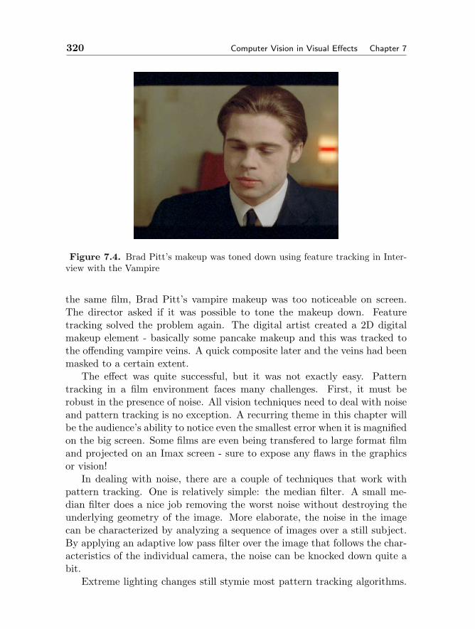
320 Computer Vision in Visual Effects Chapter 7
Figure 7.4. Brad Pitt’s makeup was toned down using feature tracking in Inter-view with the Vampire
the same film, Brad Pitt’s vampire makeup was too noticeable on screen.The director asked if it was possible to tone the makeup down. Featuretracking solved the problem again. The digital artist created a 2D digitalmakeup element - basically some pancake makeup and this was tracked tothe offending vampire veins. A quick composite later and the veins had beenmasked to a certain extent.
The effect was quite successful, but it was not exactly easy. Patterntracking in a film environment faces many challenges. First, it must berobust in the presence of noise. All vision techniques need to deal with noiseand pattern tracking is no exception. A recurring theme in this chapter willbe the audience’s ability to notice even the smallest error when it is magnifiedon the big screen. Some films are even being transfered to large format filmand projected on an Imax screen - sure to expose any flaws in the graphicsor vision!
In dealing with noise, there are a couple of techniques that work withpattern tracking. One is relatively simple: the median filter. A small me-dian filter does a nice job removing the worst noise without destroying theunderlying geometry of the image. More elaborate, the noise in the imagecan be characterized by analyzing a sequence of images over a still subject.By applying an adaptive low pass filter over the image that follows the char-acteristics of the individual camera, the noise can be knocked down quite abit.
Extreme lighting changes still stymie most pattern tracking algorithms.
Section 7.4. Optical Flow 321
A high degree of specular reflection blows out most underlying informationin the image and is quite difficult to deal with in a pattern track. Flashes oflightning or other extreme lighting changes also produce bloom on the imagethat will change the geometry of the pattern being tracked. At this pointthere is no recourse but to track the offending frames by hand.
7.4 Optical Flow
Recently, over the last 5 years, optical flow techniques have really started tomake a big impact on the film industry. In fact there are a couple of com-panies that do fairly well selling software based on optical flow techniques.
Optical flow is the 2D motion of the features in an image sequence, fromone frame to the next [1, 10]. Consider a pattern track centered on everypixel. After an optical flow analysis of an image sequence, a secondaryframe is generated for every original image in the sequence. This new imagedoes not contain colors, but rather a 2D vector for each pixel. This vectorrepresents the motion of the feature seen through the pixel from one frameto the next.
In an ideal case, if one were to take the pixels of the image n and movethem all along their individual motion vectors, an exact replica of image n+1will be created. The pixels in image n have been pushed around to makeimage n+1.
Of course, things never work out that perfectly, but it is possible tosee the power of such information. The first application of optical flowfollows naturally: change the timing of a sequence of images. If the directorshot a sequence using a standard film camera at normal speed, 24 framesare exposed per second. It happens occasionally that the director wants tochange the speed of the film, either slow it down or speed it up. Optical flowhelps in either case.
Slowing down a image sequence is relatively easy. If the director wantedto see the shot as if it was filmed at 48 frames per second, one simply dupli-cates each frame of film. This was what was done before the advent of digitalimage manipulation. A single film negative was printed onto two frames ofprint film. Playing the resulting film back resulted in slow motion. However,it also looked a little jerky. The film pauses for 2 24ths of a second and it is anoticeable effect. The solution was to generate in-between frames that wereblends of image n and image n+1. Again, this was done during the printingprocess: the in-between frames are generated by exposing the print film withthe n and n+1 negative frames for only half the exposure time each. Thiscreated an in-between frame that looked different than the original frames,

322 Computer Vision in Visual Effects Chapter 7
but also looked pretty bad. It was a double exposure of two different imagesand exhibits quite a bit of strobing and streaking.
Optical flow comes to the rescue. In the explanation above, it was shownthat by moving the pixels along the optical flow motion vectors, a new imagecan be generated. By scaling the motion vectors by half, the new image isexactly between the two original images. This new image typically looksquite a bit better than a blend of the neighboring images, it does not exhibitany of the blurred or double exposed edges. It also has the advantage in thatit can be used to slow the original sequence down by any factor. New imagescan be generated by scaling the motion vectors by any value from 0.0 to 1.0.
But pause a moment. It was stated earlier that if the pixels are pushedalong their motion vectors, the image at n+1 can be created from the pixelsthat make up image n. Unfortunately, it is not that easy. The motion vectorstypically go in all directions and sometimes neighboring motion vectors di-verge or converge. There is no guarantee that the pixels in image n+1 will beall filled by simply following the motion of the pixels. Instead, the operationof creating the in-between image is a “pixel pull” operation. For each pixelin image n+1, a search is done to find the motion vector that will land in thecenter of the pixel. This motion vector will probably be the motion vectorlocated at a sub-pixel location that is the result of an interpolation betweenthe 4 neighboring pixels. A search is made in the local neighborhood of thedestination pixel to find a likely starting pixel location in image n. Then agradient descent is used to compute the exact sub-pixel location, that whenadded to the interpolated motion vector lands on the center of the desiredpixel.
But there is more! Interpolating the color of the subpixel will lead tosampling and aliasing artifacts. In fact if the motion vectors converge - thecolors of a group of pixels all end up at one pixel in image n+1 - the originalpixels should be filtered to generate an accurate pixel color. What is typicallydone is that the previous backwards tracing is done from the 4 corners ofthe pixel. This creates a 4 sided polygonal area that is sampled and filtered.These results create a superior in-between image.
Speeding up a sequence of images is just as straightforward, with a slighttwist. Consider the problem of speeding up the action by a factor of two.In that case, it is desired to make it look like the action was filmed with acamera that ran at 12 frames a second. It should be easy, right? Simplythrow away every other frame from the original sequence! This works fine,with one problem: motion blur. The objects in the images are now supposedto be moving twice as fast and the motion blur recorded on the images lookslike it was filmed with a 24 frames per second camera. This produces the
Section 7.4. Optical Flow 323
strobing, harsh effect normally associated with sped up film.Optical flow comes to the rescue in this case as well. The motion vectors
associated with each pixel can be used to streak the images so that themotion blur appears correct. Like the sampling issue before, blurring animage according to optical flow motion has some hidden issues. The easy,but incorrect, way to add motion blur to the image is to use the motionvector to create a convolution kernel. The entries in the convolution kernelthat are within a certain distance from the motion vector are given a weightbased on a gaussian falloff. The final kernel is normalized and convolvedwith the image to produce the resultant pixel. This is done for each pixel inthe image. This technique certainly blurs the image in a complex directionalsense, but it does not quite produce correct motion blur. (It is reasonablyfast - it does require a different kernel computation at every pixel - and quiteacceptable in some situations.)
This method, as mentioned, is incorrect. Consider this example: a modelof a spaceship has been filmed on the set with a black background behind it.After the shoot, it is decided to add more motion blur to the shot - maybeit makes the shot more dynamic or something. So, somehow motion vectorsfor each pixel are computed. It need not be optical flow in this case. Sincethe model is rigid, it is possible to use the motion of the motion control rig ortracking the motion of the model to generate a reproduction of the model shotin the computer. This can then be rendered where instead of writing out thecolor of every pixel, the pixels contain the motion vector. Whether createdby optical flow or some rendering technique, assume the pixels contain the2D motion vector of the feature under the pixel. Now, consider what ishappening at the edge of the model. A pixel covering the edge of the modelwill have the appropriate motion vector, but the neighboring pixel that onlycovers background contains no motion at all! The background is black, andeven if the camera is moving, it will be impossible to detect the motion. Theproblem becomes evident at this point. Using the previous technique to addmotion blur, if the spaceship is moving fast, the pixels covering the spaceshipwill be heavily blurred. The pixels right next to the spaceship will have noblurring at all. This causes a massive visual discontinuity that audiences(and visual effects supervisors) are sure to notice.
There is a (mostly) correct solution to this: instead of blurring the pixels,distribute the energy of the pixels along the motion vector. This gets a littlemore complicated in that the motion vectors are converging and divergingin places. This caused problems in interpolating images, and it causes prob-lems adding motion blur. Basically, the color of a pixel is distributed alongthe motion vector path from the pixel. Doing the naive approach of simply
324 Computer Vision in Visual Effects Chapter 7
adding a fraction of the pixel’s color to the pixels that intersect the pathproduces bright and dark streaks in the motion blur where the vector con-verge and diverge. Rather, one has to use the interpolated motion vectorsat each corner to create a motion polygon of converge. Then, the color isadded to each pixel under the motion polygon, using a weighting that is thearea of coverage of the individual covered pixel divided by the total area ofthe motion polygon. This produces lovely motion blur, at quite a cost incompute time. In the reality of visual effects, we try to get away with thecheap solution for motion blur, knowing that we can always pay the pricefor the more accurate version of motion blur.
The previous paragraphs seem to indicate that optical flow is a robust,trustworthy algorithm. This is not the case. Optical flow gets terribly con-fused with pixels that contain features that disappear (or appear) in thespace of one frame. This is commonly referred to as fold-over. Also, spec-ular highlights and reflections in objects can fool even the best optical flowalgorithm. And most optical flow algorithms assume a certain spatial con-tinuity - one pixel moves in pretty much the same direction as its neighbor- which makes computing optical flow on complicated moving objects likewater or blowing tree leaves quite difficult.
There are many solutions to these problems. If the fold-over areas canbe found, they can be dealt with by predicting the motion of the pixels fromprevious or following frames. Sequences of images are often analyzed bothforwards and backwards, where the pixel motion vectors do not match upis usually a good indication of fold-over. Most optical flow algorithms alsocompute an indication of confidence in the flow for a pixel or an area. Wherefold-over areas are indicated, the discontinuity in the vectors is encouragedrather than avoided. And interpolating the pixels for in-between frames isdone by recognizing that the pixel will either be disappearing or appearingand interpolating in the appropriate direction.
Optical flow is not just for image manipulation. It is increasingly beingused to extract information about the image. In 2002, Yung-Yu Chung et alpublished an influential paper titled “Video Matting of Complex Scenes” [2].The techniques in this paper have made an impact on the film industry:it is now quite a bit easier to extract a matte from an object that wasnot filmed in front of a blue screen. The paper describes a technique forcomputing the matte based on Bayesian likelihood estimates. Optical flowcomes into play by pushing the initial estimate of the matte (or in this case,the trimap - a segmenting of the image into foreground, background andunknown elements) around as the contents of the image moves. It uses thesame technique as described above for computing an in-between image, but
Section 7.5. Camera Tracking and Structure from Motion 325
this time applied to the trimap image. Many visual effects companies haveimplemented compositing techniques based on this paper.
Additionally, ESC Entertainment used optical flow to help in reconstruct-ing the facial motion of the actors in the movies “Matrix Reloaded” and“Matrix Revolutions”. They filmed an actor in front of a blue screen withthree (or more) synced cameras. Instead of using traditional stereo tech-niques, which have problems with stereo correspondence, the artists placeda 3D facial mask on the face of the actor in each film sequence. This wasrelatively easy to do for the first frame of the film - the actor’s face had notdeformed from the digitized mask. The sequences of film were analyzed foroptical flow. Then the vertices of the mask were moved in 2D according tothe optical flow. Since each vertex could be seen in 2 or more camera views,the new 3D position of the vertex can be calculated by triangulation. Doingthis for each vertex on every frame produced quite clean moving, deform-ing masks of face’s of the actors. This avoided any stereo correspondenceproblem!
7.5 Camera Tracking and Structure from Motion
With the advent of computer vision techniques in visual effects, directorsfound that they could move the camera all over the place and the effects crewcould still insert digital effects into the image. So, naturally, film directorsran with the ability and never looked back. Now all the large effects shopshave dedicated teams of computer vision artists. Almost every shot is trackedin one way or another.
In the computer vision community, the world space location of the camerais typically referred to as the camera’s extrinsic parameters. Computingthese parameters from information in an image or images is typically referredto as “camera tracking” in the visual effects industry. In computer vision thistask has different names depending on how you approach the solution to theproblem: “camera calibration”, “pose estimation”, “structure from motion”and more. All the latest techniques are available to the artists computingthe camera motion.
The overriding concern of the artists is accuracy. Once a shot gets as-signed to an artist, the artist produces versions of the camera track thatare rendered as wireframe over the background image. Until the wireframeobjects line up exactly the artist must continually revisit the sequence, ad-justing and tweaking the motion curves of the camera or the objects.
A camera track starts its life on the set. As mentioned before, the dataintegration team gathers as much information as is practical. At the min-
326 Computer Vision in Visual Effects Chapter 7
imum, a camera calibration chart is photographed, but often a survey ofkey points is created or the set is photographed with a reference object sothat photogrammetry can be used to determine the 3D location of points onthe set. This data is used to create a polygonal model of the points on theset. (This model is often quite hard to decipher. It typically only has keypoints in the set and they are connected in a rough manner. But it is usuallyenough to guide the tracking artist.)
The images from the shot are “brought on-line” - either scanned fromthe original film or transfered from the high definition digital camera. Also,any notes from the set are transcribed to a text file and associated with theimages.
Before the tracking is begun, the lens distortion must be dealt with.While the lenses used in film making are quite extraordinary, they still con-tain a certain amount of radial distortion on the image. Fixed lenses arequite good, but zoom lenses and especially anamorphic lens setups are quitenotorious for the distortion they contain. In fact, for an anamorphic zoomlens, the distortion is quite hard to characterize. For the most part, the in-trinsic parameters of the lens are easily computed from the calibration chartson set. For more complicated lenses where the standard radial lens distortionequations do not accurately model the behavior of the lens, the distortion ismodeled by hand. A correspondence between the grid shot through the lensand an ideal grid is built and used to warp the image into the ideal state.
However the lens distortion is computed, the images are warped to pro-duce “straightened images” which approximate what would be seen througha pinhole camera. These images are used on-line throughout the tracking,modeling and animation process. The original images are only used whenthe final results are composited with the rendered components of the shot.This seems like an unnecessary step, surely the intrinsic parameters of thelens can be incorporated into the camera model? The problem is that theseimages are not just used for tracking, but also as background images in theanimation packages that the artists use. And in those packages, a simpleOpenGL pinhole camera model is the only one available. So, if the originalimages were used to track the camera motion and the tracking package uses acomplicated camera model that includes radial (or arbitrary) lens distortion,the line-up would look incorrect when viewed through a standard animationpackage that does not support a more complicated camera model.
The implications of this are twofold. One, two different sets of imagesmust be stored on disk, the original and the straightened version. Secondly,the artists must render their CG elements at a higher resolution becausethey will eventually be warped to fit the original images and this will soften
Section 7.5. Camera Tracking and Structure from Motion 327
Figure 7.5. Snapshot of a boat/car chase in the movie “xXx”. Left: Original;Right: Final composite image with digital hydrofoils inserted.
The artist assigned to the shot will use either an in-house computer visionprogram or one of many commercially available packages. For the most part,these programs have similar capabilities. They can perform pattern trackingand feature detection, they can set up a constraint system and then solvefor the location of the camera or moving rigid objects in the scene. Andrecently, most of these program have added the ability to compute structurefrom motion without the aid of any surveyed information.
In the most likely scenario, the artists will begin with the sequence ofimages and the surveyed geometry. Correspondences between the points onthe geometry and the points in the scene are made and an initial cameralocation is determined. Typically, the data integration team has computedthe intrinsic parameters of the camera based on the reference grid shot withthe lens.
Once the initial pose is determined, the points associated with each pointon the reference geometry are tracked in 2D over time. Pattern trackers areused to do this, though when the pattern tracks fail, the artist will oftentrack the images by hand.
Why would pattern tracks fail? One of the most common reasons is thatfeature points in the scene - the ones that are easy to digitize with a totalstation - are often not the best points to camera track: corners of objects.Corners can be difficult to pattern track because of the large amount ofchange that the pattern undergoes as the camera rotates around the corner.And often the background behind the corner will contribute to confusion ofthe pattern tracking algorithm. Corner detection algorithms can pick themout, but the sub-pixel precision of these algorithms is not as high as onesbased on cross correlation template matching.
Motion blur poses many problems for the tracking artist. Pattern trackers
328 Computer Vision in Visual Effects Chapter 7
often fail in the presence of motion blur. And even if the artist is forced totrack the pattern by hand, it can be difficult to determine where a featurelies on the image if it is blurred over many pixels. Recently, the artistsat Digital Domain were tracking a shot for a movie called “xXx”. In theshot, the camera was mounted on a speeding car traveling down a roadparallel to a river. On the river, a hydrofoil boat was traveling alongside thecar. The effect was to replace the top of the boat with a digitally createddoomsday device and make it look like it was screaming down the riveron some nefarious mission. The first task was to track the camera motionof the car with respect to the background landscape. Then the boat wastracked as a rigid moving object with respect to the motion of the camera.Naturally, the motion blur for both cases was extreme. Automatic trackingprogram had a very difficult time due to the extreme motion of the camera.Feature points would travel nearly half way across the image in the spaceof one or two frames. Optical flow algorithms failed for the same reason.Tracking the points proved quite difficult because of the extreme streakingof the information in the image. The artists placed the point in the centerof the streak and hoped for the best.
This worked, to some extent. In this extreme example, the motion blurof the boat was, at times, so extreme that the streaks caused by the motionblur were not linear at all. The motion of tracked camera and boat wererepresented as a linear interpolation between key-frame positions at everyframe. The motion blur generated by the renderer did not match the motionblur of the background frame. It is surprising how much small detail theeye can pick up. When the artists used spline interpolation to interpolatethe camera motion and added sub-frame key-frames to correctly account forsharp camera/model motion, the digital imagery fit with the backgroundnoticeably better.
Beyond the tracking of points, digital tracking artists have many toolsavailable for a good track. The points can be weighted based on the certaintyof the points - points that are obscured by objects can still be used, eventhough one cannot see them, their position is interpolated (or guessed) andtheir uncertainty set very high. Camera pose estimation is still an optimiza-tion problem and often the position computed is the position that minimizesthe error in the correspondence of points. That being the case, removing apoint from the equation can have quite an effect to the computed location ofthe camera. This results in the dreaded “pop” in motion after a point leavesthe image. This pop can be managed by ramping the point’s uncertaintyas the point approaches leaving the image. Alternately the point can beused after it leaves the image, the artist pretends that the point’s location
Section 7.5. Camera Tracking and Structure from Motion 329
is known and this can minimize any popping.Other constraints beyond points are available in many packages. Linear
constraints are often useful, an edge on the surveyed geometry is constrainedto stay on the edge of an object in the image. Pattern trackers are able tofollow the edge of the object as easily as a point on the object.
Of course, it is not necessary to have any surveyed information. Structurefrom motion techniques can solve for the location of both the camera and the3D points in the scene without any surveyed information at all. If there is noabsolute measurement of anything on the set, there is no way for structurefrom motion algorithms to determine the absolute scale of the 3D points andcamera translation. Scale is important to digital artists, animated charactersand physical effects are built at a specific scale and having to play with thescale to get things to “look right” is not something that artists like to do.So, even when relying on structure from motion, some information - like themeasurement of a distance between two points on the set - is quite useful forestablishing the scale of the scene.
The convergence of optical flow techniques, following good features fortracks and structure from motion solvers has caused large ripples throughthe film and video production facilities. Now, with no a priori knowledgeof the set, a reasonable track and reconstruction of the set can be created- as long as the camera moves enough and enough points can be followed.Some small visual effects facilities rely on almost all structure from motionsolutions. Larger facilities are finding it to be an enormous help, but rely onmore traditional camera tracking techniques for quite a few shots. Automatictracking is automatic when it is easy.
Consider a shot where the camera is moving the camera is chasing thehero of the film down a street. At some point the camera points up to the skyand then back down to center on the main character. Typical effects mightbe to add some digital buildings to the set (or at least enhance the buildingsthat are already in the scene) and perhaps add some flying machines orcreatures chasing our hero. This makes the camera tracking particularlychallenging: the camera, when it points to the sky, will not be able to viewany track-able points. But, if building and flying objects are being added tothe scene, the camera move during that time must at least be “plausible”and certainly be smooth and not exhibit any popping motion as trackingpoints are let go. Automatic tracking techniques are generally not used onthis kind of shot because the artist will want complete control of the pointsused to compute the camera motion. The camera will be tracked for thebeginning of the shot and the end of the shot and then the camera motionfor the area where the camera is only pointing at sky or non-valid tracking
330 Computer Vision in Visual Effects Chapter 7
points (like the top of the actor’s head) is created by clever interpolation andgut feeling for what the camera was doing. Often something can be tracked,even if it is a far off cloud, and that can at least be used to determine therotation of the camera.
7.6 The Future
Camera tracking and photogrammetry are the main applications of computervision in visual effects. But new techniques are making it into visual effectsall the time.
Space carving techniques are starting to show up in visual effects. Inthe movie “Minority Report”, a 3D image of a person was projected inTom Cruise’s apartment. The camera roamed around the projection and itneeded to look like a true 3D display. The projected actor was filmed on aspecial greenscreen stage, surrounded by many synchronized video cameras.Each camera was calibrated and fixed. Since the actor was surrounded bygreenscreen, it was relatively simple to determine what part of each imagewas actor and what was background. From this a view volume was formed.The intersection of all the view volumes of all the cameras produced a convexhull of the actor. Projecting the images onto the resulting geometry produceda remarkably realistic model of the person. This is just the beginning forthis technique. At recent conferences, similar techniques are being developedto extract amazingly detailed deforming models of humans with concavitiesand everything.
It is a terribly exciting time to be involved in computer vision and visualeffects. Over the years the advantages of robust computer vision tools hasbecome evident to the artists and the management. Computer vision tech-niques allow the artists to do things that were not possible previously and ithelps them do it faster and more efficiently, which makes the managementhappy.
Editors’ note: The color version of the figures in this chapter can be foundin the accompanying DVD.
Bibliography
[1] M.J. Black and P. Anandan. “The robust estimation of multiple motions:Parametric and piecewise-smooth flow fields”. Computer Vision and ImageUnderstanding, 63(1):75–104, 1996.
[2] Y.-Y. Chuang, A. Agarwala, B. Curless, D.H. Salesin, and R. Szeliski. “Video

Bibliography 331
matting of complex scenes”. ACM Transactions on Graphics, 21(3):243–248,July 2002.
[3] P.E. Debevec. “Rendering synthetic objects into real scenes: Bridging tradi-tional and image-based graphics with global illumination and high dynamicrange photography”. Siggraph98, Annual Conference Series, pages 189–198,1998.
[4] P.E. Debevec, C.J. Taylor, and J. Malik. “Modeling and rendering architecturefrom photographs: A hybrid geometry- and image-based approach”. ComputerGraphics, Annual Conference Series, pages 11–20, 1996.
[5] H.W. Jensen, S.R. Marschner, M. Levoy, and P. Hanrahan. “A practical modelfor subsurface light transport”. Siggraph01, Annual Conference Series, pages511–518, 2001.
[6] J. Lewis. “Fast normalized cross-correlation”. Vision Interface, 1995.[7] V. Masselus, P. Dutre, F. Anrys. “The free form light stage”. Proceedings of
the 13th Eurographics Workshop on Rendering, pages 247–256, June 2002.[8] M. Pauly, R. Keiser, L.P. Kobbelt, and M. Gross. “Shape modeling with point-
sampled geometry”. ACM Transactions on Graphics, 22(3):641–650, July 2003.[9] H. Pfister, M. Zwicker, J. van Baar, and M. Gross. “Surfels: Surface elements
as rendering primitives”. Siggraph00, Annual Conference Series, pages 335-342,2000.
[10] R. Szeliski and J. Coughlin. “Spline-based image registration”. Technical ReportNo. CRL-94-1, Cambridge Research Lab., DEC, April 1994.
[11] Y. Yu, P. Debevec, J. Malik, and T. Hawkins. “Inverse global illumination:Recovering reflectance models of real scenes from photographs”. Siggraph99,Annual Conference Series, pages 215–224, Los Angeles, 1999.


Chapter 8
CONTENT-BASED IMAGERETRIEVAL: AN OVERVIEW
Theo Gevers
and Arnold W.M. Smeulders
In this chapter, we present an overview on the theory, techniques andapplications of content-based image retrieval. We choose patterns of use,image domains and computation as the pivotal building blocks of our survey.A graphical overview of the content-based image retrieval scheme is given inFig. 8.1. Derived from this scheme, we follow the data as they flow throughthe computational process, see Fig. 8.3, with the conventions indicated inFig. 8.2. In all of this chapter, we follow the review in [155] closely.
We focus on still images and leave video retrieval as a separate topic.Video retrieval could be considered as a broader topic than image retrievalas video is more than a set of isolated images. However, video retrievalcould also be considered to be simpler than image retrieval since, in additionto pictorial information, video contains supplementary information such asmotion, and spatial and time constraints e.g. video disclose its objects moreeasily as many points corresponding to one object move together and arespatially coherent in time. In still pictures the user’s narrative expression ofintention is in image selection, object description and composition. Video, inaddition, has the linear time line as an important information cue to assistthe narrative structure.
333
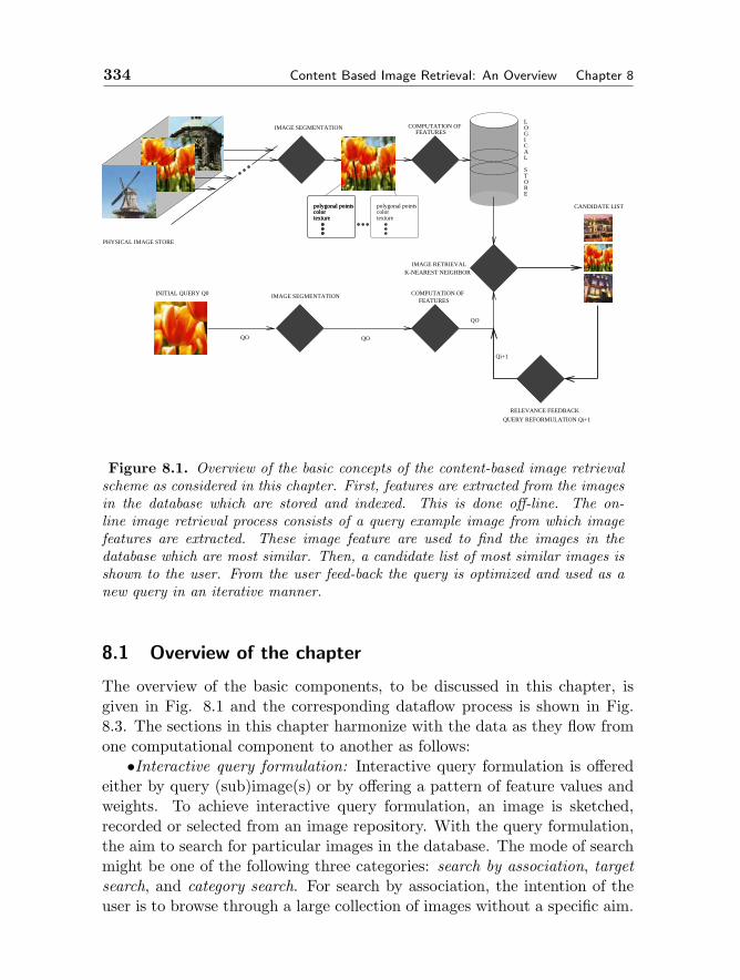
334 Content Based Image Retrieval: An Overview Chapter 8
polygonal pointscolortexture
polygonal pointscolortexture
IMAGE SEGMENTATION
IMAGE SEGMENTATION
PHYSICAL IMAGE STORE
LOGICAL
STORE
COMPUTATION OF
COMPUTATION OF
polygonal pointscolortexture
FEATURES
FEATURES
CANDIDATE LIST
RELEVANCE FEEDBACK
IMAGE RETRIEVALK-NEAREST NEIGHBOR
INITIAL QUERY Q0
QO QO
QO
QUERY REFORMULATION Qi+1
Qi+1
Figure 8.1. Overview of the basic concepts of the content-based image retrievalscheme as considered in this chapter. First, features are extracted from the imagesin the database which are stored and indexed. This is done off-line. The on-line image retrieval process consists of a query example image from which imagefeatures are extracted. These image feature are used to find the images in thedatabase which are most similar. Then, a candidate list of most similar images isshown to the user. From the user feed-back the query is optimized and used as anew query in an iterative manner.
8.1 Overview of the chapter
The overview of the basic components, to be discussed in this chapter, isgiven in Fig. 8.1 and the corresponding dataflow process is shown in Fig.8.3. The sections in this chapter harmonize with the data as they flow fromone computational component to another as follows:•Interactive query formulation: Interactive query formulation is offered
either by query (sub)image(s) or by offering a pattern of feature values andweights. To achieve interactive query formulation, an image is sketched,recorded or selected from an image repository. With the query formulation,the aim to search for particular images in the database. The mode of searchmight be one of the following three categories: search by association, targetsearch, and category search. For search by association, the intention of theuser is to browse through a large collection of images without a specific aim.

Section 8.1. Overview of the chapter 335
Figure 8.2. Data flow and symbol conventions as used in this chapter. Differentstyles of arrows indicate different data structures.
Search by association tries to find interesting images and is often applied inan iterative way by means of relevance feedback. Target search is to findsimilar (target) images in the image database. Note that ”similar image”may imply a (partially) identical image, or a (partially) identical object inthe image. The third class is category search, where the aim is to retrieve anarbitrary image which is typical for a specific class or genre (e.g. indoor im-ages, portraits, city views). As many image retrieval systems are assembledaround one of these three search modes, it is important to get more insightin these categories and their structure. Search modes will be discussed inSection 8.2.1.•Image domains: The definition of image features depends on the reper-
toire of images under consideration. This repertoire can be ordered along thecomplexity of variations imposed by the imaging conditions such as illumi-nation and viewing geometry going from narrow domains to broad domains.For images from a narrow domain there will be a restricted variability oftheir pictorial content. Examples of narrow domains are stamp collections
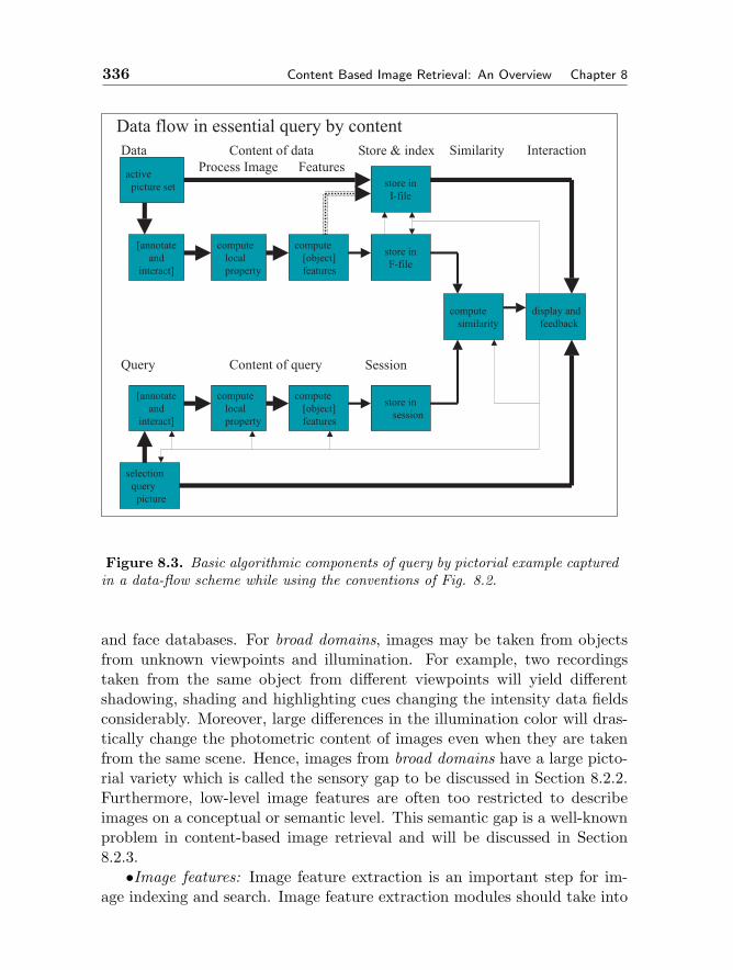
336 Content Based Image Retrieval: An Overview Chapter 8
Figure 8.3. Basic algorithmic components of query by pictorial example capturedin a data-flow scheme while using the conventions of Fig. 8.2.
and face databases. For broad domains, images may be taken from objectsfrom unknown viewpoints and illumination. For example, two recordingstaken from the same object from different viewpoints will yield differentshadowing, shading and highlighting cues changing the intensity data fieldsconsiderably. Moreover, large differences in the illumination color will dras-tically change the photometric content of images even when they are takenfrom the same scene. Hence, images from broad domains have a large picto-rial variety which is called the sensory gap to be discussed in Section 8.2.2.Furthermore, low-level image features are often too restricted to describeimages on a conceptual or semantic level. This semantic gap is a well-knownproblem in content-based image retrieval and will be discussed in Section8.2.3.•Image features: Image feature extraction is an important step for im-
age indexing and search. Image feature extraction modules should take into
Section 8.1. Overview of the chapter 337
account whether the image domain is narrow or broad. In fact, they shouldconsider to which of the imaging conditions they should be invariant to such achange in viewpoint, object pose, and illumination. Further, image featuresshould be concise and complete and at the same having high discrimina-tive power. In general, a tradeoff exists between the amount of invarianceand selectivity. In Section 8.3, a taxonomy on feature extraction modules isgiven from an image processing perspective. The taxonomy can be used toselect the proper feature extraction method for a specific application basedon whether images come from broad domains and which search goals are athand (target/category/associate search). In Section 8.3.1, we first focus oncolor content descriptors derived from image processing technology. Vari-ous color based image search methods will be discussed based on differentrepresentation schemes such as color histograms, color moments, color edgeorientation, and color correlograms. These image representation schemes arecreated on the basis of RGB, and other color systems such as HSI and CIEL∗a∗b∗. For example, the L∗a∗b∗ space has been designed to conform to thehuman perception of color similarity. If the appreciation of a human observerof an object is based on the perception of certain conspicuous items in theimage, it is natural to direct the computation of broad domain features tothese points and regions. Similarly, a biologically plausible architecture [84]of center-surround processing units is likely to select regions which humanswould also focus on first. Further, color models are discussed which arerobust to a change in viewing direction, object geometry and illumination.Image processing for shape is outlined in Section 8.3.2. We focus on localshape which are image descriptors capturing salient details in images. Fi-nally, in Section 8.3.3, our attention is directed towards texture and a reviewis given on texture features describing local color characteristics and theirspatial layout.•Representation and indexingRepresentation and indexing will be discussed in Section 8.4. In gen-
eral, the image feature set is represented by vector space, probabilistic orlogical models. For example, for the vector space model, weights can beassigned corresponding to the feature frequency giving the well-known his-togram form. Further, for accurate image search, it is often desirable toassign weights in accordance to the importance of the image features. Theimage feature weights used for both images and queries can be computedas the product of the features frequency multiplied by the inverse collectionfrequency factor. In this way, features are emphasized having high featurefrequencies but low overall collection frequencies. More on feature accumu-lation and representation is discussed in Section 8.4.2. In addition to feature
338 Content Based Image Retrieval: An Overview Chapter 8
representation, indexing is required to speed up the search process. Indexingtechniques include adaptive histogram binning, signature files, and hashing.Further, tree-based indexing schemes have been developed for indexing thestored images so that similar images can be identified efficiently at someadditional costs in memory, such as a k-d tree, R*-tree or a SS-tree, [69] forexample.
Throughout the chapter, a distinction is made between weak and strongsegmentation. Weak segmentation is a local grouping approach usually focus-ing on conspicuous regions such as edges, corners and higher-order junctions.In Section 8.4.4, various methods are discussed to achieve weak segmenta-tion. Strong segmentation is the extraction of the complete contour of anobject in an image. Obviously, strong segmentation is far more difficultthan weak segmentation and is hard to achieve if not impossible for broaddomains.•Similarity and searchThe actual matching process can be seen as a search for images in the
stored image set closest to the query specification. As both the query andthe image data set is captured in feature form, the similarity function oper-ates between the weighted feature sets. To make the query effective, closeattention has to be paid to the selection of the similarity function. A propersimilarity function should be robust to object fragmentation, occlusion andclutter by the presence of other objects in the view. For example, it is knownthat the mean square and the Euclidean similarity measure provides accu-rate retrieval without any object clutter [59] [162]. A detailed overview onsimilarity and search is given in Section 8.5.•Interaction and LearningVisualization of the feature matching results gives the user insight in
the importance of the different features. Windowing and information dis-play techniques can be used to establish communications between systemand user. In particular, new visualization techniques such as 3D virtualimage clouds can used to designate certain images as relevant to the user’srequirements. These relevant images are then further used by the systemto construct subsequent (improved) queries. Relevance feedback is an auto-matic process designed to produce improved query formulations following aninitial retrieval operation. Relevance feedback is needed for image retrievalwhere users find it difficult to formulate pictorial queries. For example,without any specific query image example, the user might find it difficult toformulate a query (e.g. to retrieve an image of a car) by image sketch or byoffering a pattern of feature values and weights. This suggests that the firstsearch is performed by an initial query formulation and a (new) improved
Section 8.2. Image Domains 339
query formulation is constructed based on the search results with the goal toretrieve more relevant images in the next search operations. Hence, from theuser feedback giving negative/positive answers, the method can automati-cally learn which image features are more important. The system uses thefeature weighting given by the user to find the images in the image databasewhich are optimal with respect to the feature weighting. For example, thesearch by association allows users to refine iteratively the query definition,the similarity or the examples with which the search was started. There-fore, systems in this category are highly interactive. Interaction, relevancefeedback and learning are discussed in Section 8.6.•TestingIn general, image search systems are assessed in terms of precision, re-
call, query-processing time as well as reliability of a negative answer. Fur-ther, the relevance feedback method is assessed in terms of the number ofiterations to approach to the ground-truth. Today, more and more imagesare archived yielding a very large range of complex pictorial information. Infact, the average number of images, used for experimentation as reported inthe literature, augmented from a few in 1995 to over a hundred thousand bynow. It is important that the dataset should have ground-truths i.e. imageswhich are (non) relevant to a given query. In general, it is hard to get theseground-truths. Especially for very large datasets. A discussion on systemperformance is given in Section 8.6.
8.2 Image Domains
In this section, we discuss patterns in image search applications, the reper-toire of images, the influence of the image formation process, and the seman-tic gap between image descriptors and the user.
8.2.1 Search modes
We distinguish three broad categories of search modes when using a content-based image retrieval system, see Fig. 8.4.• There is a broad variety of methods and systems designed to browse
through a large set of images from unspecified sources, which is called searchby association. At the start, users of search by association have no specificaims other than to find interesting images. Search by association often im-plies iterative refinement of the search, the similarity or the examples withwhich the search was initiated. Systems in this category are highly inter-active, where the query specification may be defined by sketch [28] or byexample images. The oldest realistic example of such a system is probably
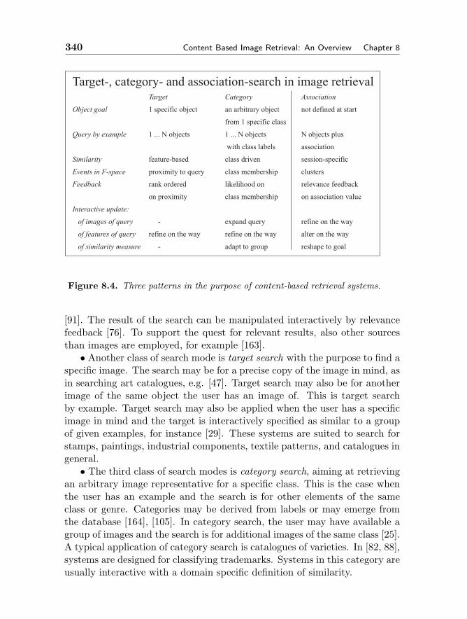
340 Content Based Image Retrieval: An Overview Chapter 8
Figure 8.4. Three patterns in the purpose of content-based retrieval systems.
[91]. The result of the search can be manipulated interactively by relevancefeedback [76]. To support the quest for relevant results, also other sourcesthan images are employed, for example [163].• Another class of search mode is target search with the purpose to find a
specific image. The search may be for a precise copy of the image in mind, asin searching art catalogues, e.g. [47]. Target search may also be for anotherimage of the same object the user has an image of. This is target searchby example. Target search may also be applied when the user has a specificimage in mind and the target is interactively specified as similar to a groupof given examples, for instance [29]. These systems are suited to search forstamps, paintings, industrial components, textile patterns, and catalogues ingeneral.• The third class of search modes is category search, aiming at retrieving
an arbitrary image representative for a specific class. This is the case whenthe user has an example and the search is for other elements of the sameclass or genre. Categories may be derived from labels or may emerge fromthe database [164], [105]. In category search, the user may have available agroup of images and the search is for additional images of the same class [25].A typical application of category search is catalogues of varieties. In [82, 88],systems are designed for classifying trademarks. Systems in this category areusually interactive with a domain specific definition of similarity.
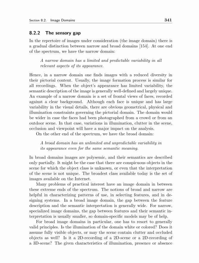
Section 8.2. Image Domains 341
8.2.2 The sensory gap
In the repertoire of images under consideration (the image domain) there isa gradual distinction between narrow and broad domains [154]. At one endof the spectrum, we have the narrow domain:
A narrow domain has a limited and predictable variability in allrelevant aspects of its appearance.
Hence, in a narrow domain one finds images with a reduced diversity intheir pictorial content. Usually, the image formation process is similar forall recordings. When the object’s appearance has limited variability, thesemantic description of the image is generally well-defined and largely unique.An example of a narrow domain is a set of frontal views of faces, recordedagainst a clear background. Although each face is unique and has largevariability in the visual details, there are obvious geometrical, physical andillumination constraints governing the pictorial domain. The domain wouldbe wider in case the faces had been photographed from a crowd or from anoutdoor scene. In that case, variations in illumination, clutter in the scene,occlusion and viewpoint will have a major impact on the analysis.
On the other end of the spectrum, we have the broad domain:
A broad domain has an unlimited and unpredictable variability inits appearance even for the same semantic meaning.
In broad domains images are polysemic, and their semantics are describedonly partially. It might be the case that there are conspicuous objects in thescene for which the object class is unknown, or even that the interpretationof the scene is not unique. The broadest class available today is the set ofimages available on the Internet.
Many problems of practical interest have an image domain in betweenthese extreme ends of the spectrum. The notions of broad and narrow arehelpful in characterizing patterns of use, in selecting features, and in de-signing systems. In a broad image domain, the gap between the featuredescription and the semantic interpretation is generally wide. For narrow,specialized image domains, the gap between features and their semantic in-terpretation is usually smaller, so domain-specific models may be of help.
For broad image domains in particular, one has to resort to generallyvalid principles. Is the illumination of the domain white or colored? Does itassume fully visible objects, or may the scene contain clutter and occludedobjects as well? Is it a 2D-recording of a 2D-scene or a 2D-recording ofa 3D-scene? The given characteristics of illumination, presence or absence
342 Content Based Image Retrieval: An Overview Chapter 8
of occlusion, clutter, and differences in camera viewpoint, determine thedemands on the methods of retrieval.
The sensory gap is the gap between the object in the world andthe information in a (computational) description derived from arecording of that scene.
The sensory gap makes the description of objects an ill-posed problem: ityields uncertainty in what is known about the state of the object. The sen-sory gap is particularly poignant when a precise knowledge of the recordingconditions is missing. The 2D-records of different 3D-objects can be identi-cal. Without further knowledge, one has to decide that they might representthe same object. Also, a 2D-recording of a 3D- scene contains informationaccidental for that scene and that sensing but one does not know what partof the information is scene related. The uncertainty due to the sensory gapdoes not only hold for the viewpoint, but also for occlusion (where essentialparts telling two objects apart may be out of sight), clutter, and illumination.
8.2.3 The semantic gap
As stated in the previous sections, content-based image retrieval relies onmultiple low-level features (e.g. color, shape and texture) describing theimage content. To cope with the sensory gap, these low-level features shouldbe consistent and invariant to remain representative for the repertoire ofimages in the database. For image retrieval by query by example, the on-lineimage retrieval process consists of a query example image, given by the useron input, from which low-level image features are extracted. These imagefeatures are used to find images in the database which are most similar to thequery image. A drawback, however, is that these low-level image features areoften too restricted to describe images on a conceptual or semantic level. Itis our opinion that ignoring the existence of the semantic gap is the cause ofmany disappointments on the performance of early image retrieval systems.
The semantic gap is the lack of coincidence between the informa-tion that one can extract from the visual data and the interpre-tation that the same data have for a user in a given situation.
A user wants to search for images on a conceptual level e.g. images containingparticular objects (target search) or conveying a certain message or genre(category search). Image descriptions, on the other hand, are derived bylow-level data-driven methods. The semantic search by the user and the
Section 8.2. Image Domains 343
low-level syntactic image descriptors may be disconnected. Association of acomplete semantic system to image data would entail, at least, solving thegeneral object recognition problem. Since this problem is yet unsolved andwill likely to stay unsolved in its entirety, research is focused on differentmethods to associate higher level semantics to data-driven observables.
Indeed, the most reasonable tool for semantic image characterizationentails annotation by keywords or captions. This converts content-basedimage access to (textual) information retrieval [134]. Common objectionsto the practice of labeling are cost and coverage. On the cost side, labelingthousands of images is a cumbersome and expensive job to the degree that thedeployment of the economic balance behind the database is likely to decrease.To solve the problem, systems presented in [140], [139] use a program thatexplores the Internet collecting images and inserting them in a predefinedtaxonomy on the basis of the text surrounding them. A similar approachfor digital libraries is taken by [19]. On the coverage side, labeling is seldomcomplete, context sensitive and, in any case, there is a significant fraction ofrequests whose semantics can’t be captured by labeling alone [7, 72]. Bothmethods will cover the semantic gap only in isolated cases.
8.2.4 Discussion
We have discussed three broad types of search categories: target search,category search and search by association. Target search is related to theclassical methods in the field of pattern matching and computer vision suchas object recognition and image matching. However, image retrieval differsfrom traditional pattern matching by considering more and more imagesin the database. Therefore, new challenges in content-based retrieval arein the huge amount of images to search among, the query specification bymultiple images, and in the variability of imaging conditions and objectstates. Category search connects to statistical pattern recognition methods.However, compared to traditional pattern recognition, new challenges arein the interactive manipulation of results, the usually very large number ofobject classes, and the absence of an explicit training phase for feature andclassifier tuning (active learning). Search by association is the most distantfrom the classical field of computer vision. It is severely hampered by thesemantic gap. As long as the gap is there, use of content-based retrieval forbrowsing will not be within the grasp of the general public as humans areaccustomed to rely on the immediate semantic imprint the moment they seean image.
An important distinction we have discussed is that between broad and
344 Content Based Image Retrieval: An Overview Chapter 8
narrow domains. The broader the domain, the more browsing or search byassociation should be considered during system set-up. The narrower thedomain, the more target search should be taken as search mode.
The major discrepancy in content-based retrieval is that the user wants toretrieve images on a semantic level, but the image characterizations can onlyprovide similarity on a low-level syntactic level. This is called the semanticgap. Furthermore, another discrepancy is that between the properties in animage and the properties of the object. This is called the sensory gap. Boththe semantic and sensory gap play a serious limiting role in the retrieval ofimages based on their content.
8.3 Image Features
Before starting the discussion on image features, it is important to keep inmind that content-based retrieval does not depend on a complete descrip-tion of the pictorial content of the image. It is sufficient that a retrievalsystem presents similar images, i.e. similar in some user defined sense. Thedescription of the content by image features should serve that goal primarily.
One such goal can be met by using invariance as a tool to deal withthe accidental distortions in the image content introduced by the sensorygap. From Section 8.2.2, it is clear that invariant features may carry moreobject-specific information than other features as they are insensitive to theaccidental imaging conditions such as illumination, object pose and cameraviewpoint. The aim of invariant image features is to identify objects nomatter from how and where they are observed at the loss of some of theinformation content.
Therefore, the degree of invariance, should be tailored to the recordingcircumstances. In general, a feature with a very wide class of invariancelooses the power to discriminate among object differences. The aim is to se-lect the tightest set of invariants suited for the expected set of non-constantconditions. What is needed in image search is a specification of the minimalinvariant conditions in the specification of the query. The minimal set of in-variant conditions can only be specified by the user as it is part of his or hersintention. For each image retrieval query a proper definition of the desiredinvariance is in order. Does the applicant wish search for the object in ro-tation and scale invariance? illumination invariance? viewpoint invariance?occlusion invariance? The oldest work on invariance in computer vision hasbeen done in object recognition as reported among others in [119] for shapeand [181] for color. Invariant description in image retrieval is relatively new,but quickly gaining ground, for a good introduction see [15], [30], [57].

Section 8.3. Image Features 345
8.3.1 Color
Color has been an active area of research in image retrieval, more than inany other branch of computer vision. Color makes the image take values ina color vector space. The choice of a color system is of great importance forthe purpose of proper image retrieval. It induces the equivalent classes tothe actual retrieval algorithm. However, no color system can be consideredas universal, because color can be interpreted and modeled in different ways.Each color system has its own set of color models, which are the parametersof the color system. Color systems have been developed for different pur-poses: 1. display and printing processes: RGB, CMY ; 2. television andvideo transmittion efficiency: Y IQ, Y UV ; 3. color standardization: XY Z;4. color uncorrelation: I1I2I3; 5. color normalization and representation:rgb, xyz; 6. perceptual uniformity: U∗V ∗W ∗, L∗a∗b∗, L∗u∗v∗; 7. and intu-itive description: HSI, HSV . With this large variety of color systems, theinevitable question arises which color system to use for which kind of imageretrieval application. To this end, criteria are required to classify the variouscolor systems for the purpose of content-based image retrieval. Firstly, animportant criterion is that the color system is independent of the underlyingimaging device. This is required when images in the image database arerecorded by different imaging devices such as scanners, camera’s and cam-recorder (e.g. images on Internet). Another prerequisite might be that thecolor system should exhibit perceptual uniformity meaning that numericaldistances within the color space can be related to human perceptual differ-ences. This is important when images are to be retrieved which should bevisually similar (e.g. stamps, trademarks and paintings databases). Also,the transformation needed to compute the color system should be linear. Anon-linear transformation may introduce instabilities with respect to noisecausing poor retrieval accuracy. Further, the color system should be com-posed of color models which are understandable and intuitive to the user.Moreover, to achieve robust image retrieval, color invariance is an impor-tant criterion. In general, images and videos are taken from objects fromdifferent viewpoints. Two recordings made of the same object from differentviewpoints will yield different shadowing, shading and highlighting cues.
Only when there is no variation in the recording or in the perceptionthan the RGB color representation is a good choice. RGB-representationsare widely in use today. They describe the image in its literal color properties.An image expressed by RGB makes most sense when recordings are madein the absence of variance, as is the case, e.g., for art paintings [72], thecolor composition of photographs [47] and trademarks [88, 39], where two
346 Content Based Image Retrieval: An Overview Chapter 8
dimensional images are recorded in frontal view under standard illuminationconditions.
A significant improvement over the RGB-color space (at least for re-trieval applications) comes from the use of normalized color representations[162]. This representation has the advantage of suppressing the intensityinformation and hence is invariant to changes in illumination intensity andobject geometry.
Others approaches use the Munsell or the L∗a∗b∗-spaces because of theirrelative perceptual uniformity. The L∗a∗b∗ color system has the propertythat the closer a point (representing a color) is to another point, the morevisual similar the colors are. In other words, the magnitude of the perceivedcolor difference of two colors corresponds to the Euclidean distance betweenthe two colors in the color system. The L∗a∗b∗ system is based on thethree dimensional coordinate system based on the opponent theory usingblack-white L∗, red-green a∗, and yellow-blue b∗ components. The L∗ axiscorresponds to the lightness where L∗ = 100 is white and L∗ = 0 is black.Further, a∗ ranges from red +a∗ to green −a∗ while b∗ ranges from yellow+b∗ to blue −b∗. The chromaticity coordinates a∗ and b∗ are insensitive tointensity and has the same invariant properties as normalized color. Careshould be taken when digitizing the non-linear conversion to L∗a∗b∗-space[117].
The HSV -representation is often selected for its invariant properties.Further, the human color perception is conveniently represented by thesecolor models where I is an attribute in terms of which a light or surfacecolor may be ordered on a scale from dim to bright. S denotes the relativewhite content of a color and H is the color aspect of a visual impression.The problem of H is that it becomes unstable when S is near zero due to thenon-removable singularities in the nonlinear transformation, which a smallperturbation of the input can cause a large jump in the transformed values[62]. H is invariant under the orientation of the object with respect to theillumination intensity and camera direction and hence more suited for objectretrieval. However, H is still dependent on the color of the illumination [57].
A wide variety of tight photometric color invariants for object retrievalwere derived in [59] from the analysis of the dichromatic reflection model.They derive for matte patches under white light the invariant color space(R−GR+G ,−B−R
B+R ,G−BG+B ), only dependent on sensor and surface albedo. For a
shiny surface and white illumination, they derive the invariant representationas |R−G|
|R−G|+|B−R|+|G−B| and two more permutations. The color models arerobust against major viewpoint distortions.
Color constancy is the capability of humans to perceive the same color
Section 8.3. Image Features 347
in the presence of variations in illumination which change the physical spec-trum of the perceived light. The problem of color constancy has been thetopic of much research in psychology and computer vision. Existing colorconstancy methods require specific a priori information about the observedscene (e.g. the placement of calibration patches of known spectral reflectancein the scene) which will not be feasible in practical situations, [48], [52], [97]for example. In contrast, without any a priori information, [73], [45] useillumination-invariant moments of color distributions for object recognition.However, these methods are sensitive to object occlusion and cluttering asthe moments are defined as an integral property on the object as one. Inglobal methods in general, occluded parts will disturb recognition. [153] cir-cumvents this problem by computing the color features from small objectregions instead of the entire object. Further, to avoid sensitivity on objectocclusion and cluttering, simple and effective illumination-independent colorratio’s have been proposed by [53], [121], [60]. These color constant modelsare based on the ratio of surface albedos rather than the recovering of theactual surface albedo itself. However, these color models assume that thevariation in spectral power distribution of the illumination can be modeledby the coefficient rule or von Kries model, where the change in the illumina-tion color is approximated by a 3x3 diagonal matrix among the sensor bandsand is equal to the multiplication of each RGB-color band by an indepen-dent scalar factor. The diagonal model of illumination change holds exactlyin the case of narrow-band sensors. Although standard video camera’s arenot equipped with narrow-band filters, spectral sharpening could be applied[46] to achieve this to a large extent.
The color ratio’s proposed by [121] are given by: N(C x1 , C x2) = Cx1−Cx2
Cx2+Cx1
and those proposed by [53] are defined by: F (C x1 , C x2) = Cx1
Cx2expressing
color ratio’s between two neighboring image locations, for C ∈ R,G,B,where x1 and x2 denote the image locations of the two neighboring pixels.
The color ratio’s of [60] are given by: M(C x11 , C x2
1 , C x12 , C x2
2 ) = Cx11 C
x22
Cx21 C
x12
expressing the color ratio between two neighboring image locations, forC1, C2 ∈ R,G,B where x1 and x2 denote the image locations of the twoneighboring pixels. All these color ratio’s are device dependent, not percep-tual uniform and they become unstable when intensity is near zero. Further,N and F are dependent on the object geometry. M has no viewing andlighting dependencies. In [55] a thorough overview is given on color modelsfor the purpose of image retrieval. Figure 8.5 shows the taxonomy of colormodels with respect to their characteristics. For more information we referto [55].
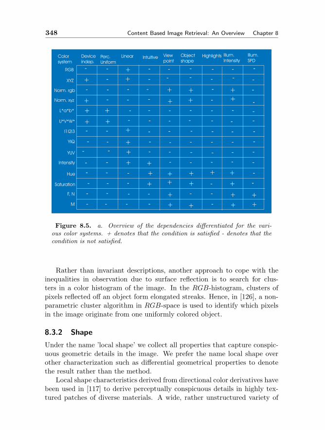
348 Content Based Image Retrieval: An Overview Chapter 8
Figure 8.5. a. Overview of the dependencies differentiated for the vari-ous color systems. + denotes that the condition is satisfied - denotes that thecondition is not satisfied.
Rather than invariant descriptions, another approach to cope with theinequalities in observation due to surface reflection is to search for clus-ters in a color histogram of the image. In the RGB-histogram, clusters ofpixels reflected off an object form elongated streaks. Hence, in [126], a non-parametric cluster algorithm in RGB-space is used to identify which pixelsin the image originate from one uniformly colored object.
8.3.2 Shape
Under the name ’local shape’ we collect all properties that capture conspic-uous geometric details in the image. We prefer the name local shape overother characterization such as differential geometrical properties to denotethe result rather than the method.
Local shape characteristics derived from directional color derivatives havebeen used in [117] to derive perceptually conspicuous details in highly tex-tured patches of diverse materials. A wide, rather unstructured variety of
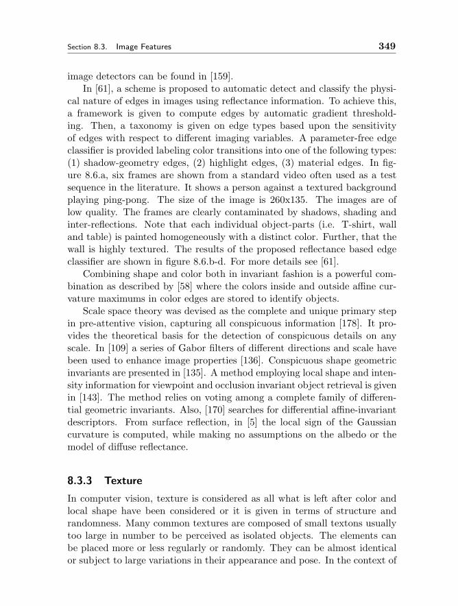
Section 8.3. Image Features 349
image detectors can be found in [159].In [61], a scheme is proposed to automatic detect and classify the physi-
cal nature of edges in images using reflectance information. To achieve this,a framework is given to compute edges by automatic gradient threshold-ing. Then, a taxonomy is given on edge types based upon the sensitivityof edges with respect to different imaging variables. A parameter-free edgeclassifier is provided labeling color transitions into one of the following types:(1) shadow-geometry edges, (2) highlight edges, (3) material edges. In fig-ure 8.6.a, six frames are shown from a standard video often used as a testsequence in the literature. It shows a person against a textured backgroundplaying ping-pong. The size of the image is 260x135. The images are oflow quality. The frames are clearly contaminated by shadows, shading andinter-reflections. Note that each individual object-parts (i.e. T-shirt, walland table) is painted homogeneously with a distinct color. Further, that thewall is highly textured. The results of the proposed reflectance based edgeclassifier are shown in figure 8.6.b-d. For more details see [61].
Combining shape and color both in invariant fashion is a powerful com-bination as described by [58] where the colors inside and outside affine cur-vature maximums in color edges are stored to identify objects.
Scale space theory was devised as the complete and unique primary stepin pre-attentive vision, capturing all conspicuous information [178]. It pro-vides the theoretical basis for the detection of conspicuous details on anyscale. In [109] a series of Gabor filters of different directions and scale havebeen used to enhance image properties [136]. Conspicuous shape geometricinvariants are presented in [135]. A method employing local shape and inten-sity information for viewpoint and occlusion invariant object retrieval is givenin [143]. The method relies on voting among a complete family of differen-tial geometric invariants. Also, [170] searches for differential affine-invariantdescriptors. From surface reflection, in [5] the local sign of the Gaussiancurvature is computed, while making no assumptions on the albedo or themodel of diffuse reflectance.
8.3.3 Texture
In computer vision, texture is considered as all what is left after color andlocal shape have been considered or it is given in terms of structure andrandomness. Many common textures are composed of small textons usuallytoo large in number to be perceived as isolated objects. The elements canbe placed more or less regularly or randomly. They can be almost identicalor subject to large variations in their appearance and pose. In the context of
350 Content Based Image Retrieval: An Overview Chapter 8
Figure 8.6. Frames from a video showing a person against a textured back-ground playing ping-pong. From left to right column. a. Original color frame.b. Classified edges. c. Material edges. d. Shadow and geometry edges.
image retrieval, research is mostly directed towards statistical or generativemethods for the characterization of patches.
Basic texture properties include the Markovian analysis dating back toHaralick in 1973 and generalized versions thereof [95, 64]. In retrieval, theproperty is computed in a sliding mask for localization [102, 66].
Another important texture analysis technique uses multi-scale auto- re-gressive MRSAR-models, which consider texture as the outcome of a deter-ministic dynamic system subject to state and observation noise [168, 110].Other models exploit statistical regularities in the texture field [9].
Wavelets [33] have received wide attention. They have often been con-sidered for their locality and their compression efficiency. Many wavelettransforms are generated by groups of dilations or dilations and rotations
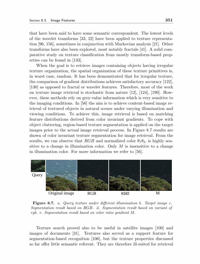
Section 8.3. Image Features 351
that have been said to have some semantic correspondent. The lowest levelsof the wavelet transforms [33, 22] have been applied to texture representa-tion [96, 156], sometimes in conjunction with Markovian analysis [21]. Othertransforms have also been explored, most notably fractals [41]. A solid com-parative study on texture classification from mostly transform-based prop-erties can be found in [133].
When the goal is to retrieve images containing objects having irregulartexture organization, the spatial organization of these texture primitives is,in worst case, random. It has been demonstrated that for irregular texture,the comparison of gradient distributions achieves satisfactory accuracy [122],[130] as opposed to fractal or wavelet features. Therefore, most of the workon texture image retrieval is stochastic from nature [12], [124], [190]. How-ever, these methods rely on grey-value information which is very sensitive tothe imaging conditions. In [56] the aim is to achieve content-based image re-trieval of textured objects in natural scenes under varying illumination andviewing conditions. To achieve this, image retrieval is based on matchingfeature distributions derived from color invariant gradients. To cope withobject cluttering, region-based texture segmentation is applied on the targetimages prior to the actual image retrieval process. In Figure 8.7 results areshown of color invariant texture segmentation for image retrieval. From theresults, we can observe that RGB and normalized color θ1θ2, is highly sen-sitive to a change in illumination color. Only M is insensitive to a changein illumination color. For more information we refer to [56].
Query
Original image RGB Mθ1θ2
Figure 8.7. a. Query texture under different illumination b. Target image c.Segmentation result based on RGB. d. Segmentation result based on variant ofrgb. e. Segmentation result based on color ratio gradient M .
Texture search proved also to be useful in satellite images [100] andimages of documents [31]. Textures also served as a support feature forsegmentation-based recognition [106], but the texture properties discussedso far offer little semantic referent. They are therefore ill-suited for retrieval

352 Content Based Image Retrieval: An Overview Chapter 8
applications in which the user wants to use verbal descriptions of the image.Therefore, in retrieval research, in [104] the Wold features of periodicity,directionality, and randomness are used, which agree reasonably well withlinguistic descriptions of textures as implemented in [127].
8.3.4 Discussion
First of all, image processing in content-based retrieval should primarily beengaged in enhancing the image information of the query, not on describingthe content of the image in its entirety.
To enhance the image information, retrieval has set the spotlights oncolor, as color has a high discriminatory power among objects in a scene,much higher than gray levels. The purpose of most image color process-ing is to reduce the influence of the accidental conditions of the scene andsensing (i.e. the sensory gap). Progress has been made in tailored colorspace representation for well-described classes of variant conditions. Also,the application of geometrical description derived from scale space theorywill reveal viewpoint and scene independent salient point sets thus openingthe way to similarity of images on a few most informative regions or points.
In this chapter, we have made a separation between color, local geometryand texture. At this point it is safe to conclude that the division is anartificial labeling. For example, wavelets say something about the local shapeas well as the texture, and so may scale space and local filter strategiesdo. For the purposes of content-based retrieval an integrated view on color,texture and local geometry is urgently needed as only an integrated viewon local properties can provide the means to distinguish among hundreds ofthousands different images. A recent advancement in that direction is thefusion of illumination and scale invariant color and texture information into aconsistent set of localized properties [74]. Also in [16], homogeneous regionsare represented as collections of ellipsoids of uniform color or texture, butinvariant texture properties deserve more attention [167] and [177]. Furtherresearch is needed in the design of complete sets of image properties withwell-described variant conditions which they are capable of handling.
8.4 Representation and Indexing
In the first subsection, we discuss the ultimate form of spatial data by group-ing the data into object silhouettes, clusters of points or point-sets. In thenext subsection, we leave the spatial domain, to condense the pictorial in-formation into feature values.
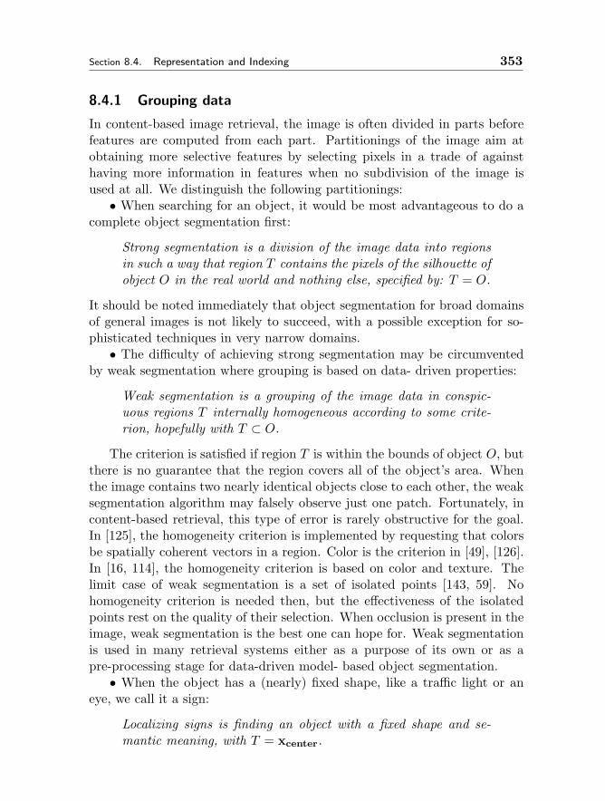
Section 8.4. Representation and Indexing 353
8.4.1 Grouping data
In content-based image retrieval, the image is often divided in parts beforefeatures are computed from each part. Partitionings of the image aim atobtaining more selective features by selecting pixels in a trade of againsthaving more information in features when no subdivision of the image isused at all. We distinguish the following partitionings:• When searching for an object, it would be most advantageous to do a
complete object segmentation first:
Strong segmentation is a division of the image data into regionsin such a way that region T contains the pixels of the silhouette ofobject O in the real world and nothing else, specified by: T = O.
It should be noted immediately that object segmentation for broad domainsof general images is not likely to succeed, with a possible exception for so-phisticated techniques in very narrow domains.• The difficulty of achieving strong segmentation may be circumvented
by weak segmentation where grouping is based on data- driven properties:
Weak segmentation is a grouping of the image data in conspic-uous regions T internally homogeneous according to some crite-rion, hopefully with T ⊂ O.
The criterion is satisfied if region T is within the bounds of object O, butthere is no guarantee that the region covers all of the object’s area. Whenthe image contains two nearly identical objects close to each other, the weaksegmentation algorithm may falsely observe just one patch. Fortunately, incontent-based retrieval, this type of error is rarely obstructive for the goal.In [125], the homogeneity criterion is implemented by requesting that colorsbe spatially coherent vectors in a region. Color is the criterion in [49], [126].In [16, 114], the homogeneity criterion is based on color and texture. Thelimit case of weak segmentation is a set of isolated points [143, 59]. Nohomogeneity criterion is needed then, but the effectiveness of the isolatedpoints rest on the quality of their selection. When occlusion is present in theimage, weak segmentation is the best one can hope for. Weak segmentationis used in many retrieval systems either as a purpose of its own or as apre-processing stage for data-driven model- based object segmentation.• When the object has a (nearly) fixed shape, like a traffic light or an
eye, we call it a sign:
Localizing signs is finding an object with a fixed shape and se-mantic meaning, with T = xcenter.
354 Content Based Image Retrieval: An Overview Chapter 8
Signs are helpful in content based retrieval as they deliver an immediate andunique semantic interpretation.• The weakest form of grouping is partitioning:
A partitioning is a division of the data array regardless of thedata, symbolized by: T = O.
The area T may be the entire image, or a conventional partitioning as thecentral part of the image against the upper, right, left and lower parts [75].The feasibility of fixed partitioning comes from the fact that image are cre-ated in accordance with certain canons or normative rules, such as placingthe horizon about 2/3 up in the picture, or keeping the main subject in thecentral area. This rule is often violated, but this violation, in itself, has se-mantic significance. Another possibility of partitioning is to divide the imagein tiles of equal size and summarize the dominant feature values in each tile[129].
8.4.2 Features accumulation
In the computational process given in Fig. 8.3, features are calculated next.The general class of accumulating features aggregate the spatial informationof a partitioning irrespective of the image data. A special type of accumu-lative features are the global features which are calculated from the entireimage. Fj (see Fig. 8.2) is the set of accumulative features or a set of accu-mulative features ranked in a histogram. Fj is part of feature space F . Tjis the partitioning over which the value of Fj is computed. In the case ofglobal features Tj=void represents the image, otherwise Tj represents a fixedtiling of the image. The operator h may hold relative weights, for exampleto compute transform coefficients.
A simple but very effective approach to accumulating features is to usethe histogram, that is the set of features F(m) ordered by histogram indexm.
One of the earlier approaches to color-based image matching, using thecolor at pixels directly as indices, has been proposed by Swain and Ballard[162]. If the RGB or normalized color distributions of two images are globallysimilar, the matching rate is high. The work by Swain and Ballard has hadan enormous impact on color-based histogram matching resulting in manyhistogram variations.
For example, the QBIC system [42] allows for a user-defined computationof the histogram by the introduction of variable k denoting the number ofbins of the histogram. Then, for each 3xk cells, the average modified Munsell
Section 8.4. Representation and Indexing 355
color is computed together with the five most frequently occurring colors.Using a standard clustering algorithm they obtain k super cells resulting inthe partitioning of the color system.
In [58] various color invariant features are selected to construct colorpattern-cards. First, histograms are created in a standard way. Because thecolor distributions of histograms depend on the scale of the recorded object(e.g. distance object-camera), they define color pattern-cards as thresholdedhistograms. In this way, color pattern-cards are scale-independent by indi-cating whether a particular color model value is substantially present in animage or not. Matching measures are defined, expressing similarity betweencolor pattern-cards, robust to a substantial amount of object occlusion andcluttering. Based on the color pattern-cards and matching functions, a hash-ing scheme is presented offering run-time image retrieval independent of thenumber of images in the image database.
In the ImageRover system, proposed by [147], the L∗u∗v∗ color space isused where each color axis has been split into 4 equally sized bins resultingin a total of 64 bins. Further, [37] uses the L∗a∗b∗ system to compute theaverage color and covariance matrix of each of the color channels. [158] usestheHSV color space to obtain a partition into 144 bins giving more emphasison hue H than value V and saturation I. Further, [4] also focuses on theHSV color space to extract regions of dominant colors. To obtain colorswhich are perceptually the same but still being distinctive, [165] proposesto partition the RGB color space into 220 subspaces. [36] computes theaverage color describing a cell of a 4x4 grid which is superimposed on theimage. [149] uses the L∗a∗b∗ color space because the color space consists ofperceptually uniform colors, which better matches the human perception ofcolor. [65] roughly partitions the Munsell color space into eleven color zones.Similar partitioning have been proposed by [29] and [24].
Another approach, proposed by [161], is the introduction of the cumu-lative color histogram which generate more dense vectors. This enables tocope with coarsely quantized color spaces. [186] proposes a variation of thecumulative histograms by applying cumulative histograms to each sub-space.
Other approaches are based on the computation of moments of each colorchannel. For example, [6] represents color regions by the first three momentsof the color models in the HSV -space. Instead of constructing histogramsfrom color invariants, [73], [45] propose the computation of illumination-invariant moments from color histograms. In a similar way, [153] computesthe color features from small object regions instead of the entire object.
[85] proposes to use integrated wavelet decomposition. In fact, the colorfeatures generate wavelet coefficients together with their energy distribu-
356 Content Based Image Retrieval: An Overview Chapter 8
tion among channels and quantization layers. Similar approaches based onwavelets have been proposed by [175], [101].
All of this is in favor of the use of histograms. When very large data setsare at stake, plain histogram comparison will saturate the discrimination.For a 64-bin histogram, experiments show that for reasonable conditions,the discriminatory power among images is limited to 25,000 images [160].To keep up performance, in [125], a joint histogram is used providing dis-crimination among 250,000 images in their database rendering 80% recallamong the best 10 for two shots from the same scene using simple features.Other joint histograms add local texture or local shape [68], directed edges[87], and local higher order structures [47].
Another alternative is to add a dimension representing the local distance.This is the correlogram [80], defined as a 3- dimensional histogram where thecolors of any pair are along the first and second dimension and the spatialdistance between them along the third. The autocorrelogram defining thedistances between pixels of identical colors is found on the diagonal of thecorrelogram. A more general version is the geometric histogram [1] with thenormal histogram, the correlogram and several alternatives as special cases.This also includes the histogram of the triangular pixel values reported tooutperform all of the above as it contains more information.
A different view on accumulative features is to demand that all infor-mation (or all relevant information) in the image is preserved in the featurevalues. When the bit-content of the features is less than the original image,this boils down to compression transforms. Many compression transformsare known, but the quest is for transforms simultaneously suited as retrievalfeatures. As proper querying for similarity is based on a suitable distancefunction between images, the transform has to be applied on a metric space.And, the components of the transform have to correspond to semanticallymeaningful characteristics of the image. And, finally, the transform shouldadmit indexing in compressed form yielding a big computational advantageover having the image be untransformed first. [144] is just one of manywhere the cosine-based JPEG-coding scheme is used for image retrieval. TheJPEG-transform fulfills the first and third requirement but fails on a lackof semantics. In the MPEG-standard the possibility to include semantic de-scriptors in the compression transform is introduced [27]. For an overviewof feature indexes in the compressed domain, see [108]. In [96], a waveletpacket was applied to texture images and, for each packet, entropy and en-ergy measures were determined and collected in a feature vector. In [83],vector quantization was applied in the space of coefficients to reduce its di-mensionality. This approach was extended to incorporate the metric of the
Section 8.4. Representation and Indexing 357
color space in [141]. In [86] a wavelet transform was applied independently tothe three channels of a color image, and only the sign of the most significantcoefficients is retained. In [3], a scheme is offered for a broad spectrum ofinvariant descriptors suitable for application on Fourier, wavelets and splinesand for geometry and color alike.
8.4.3 Feature accumulation and image partitioning
The lack of spatial information for methods based on feature accumula-tion might yield lower retrieval accuracy. As for general image databases,a manual segmentation is not feasible due to the sensory gap, a simple ap-proach is to divide images into smaller sub-images and then index them. Thisis known as fixed partitioning. Other systems use a segmentation scheme,prior to the actual image search, to partition each image into regions. Nearlyall region-based partitioning schemes use some kind of weak segmentationdecomposing the image into coherent regions rather than complete objects(strong segmentation).
Fixed Partitioning
The simplest way is to use a fixed image decomposition in which an image ispartitioned into equally sized segments. The disadvantage of a fixed parti-tioning is that blocks usually do not correspond with the visual content of animage. For example, [65] splits an image into nine equally sized sub-images,where each sub-region is represented by a color histogram. [67] segmentsthe image by a quadtree, and [99] uses a multi-resolution representation ofeach image. [36] also uses a 4x4 grid to segment the image. [148] partitionsimages into three layers, where the first layer is the whole image, the secondlayer is a 3x3 grid and the third layer a 5x5 grid. A similar approach isproposed by [107] where three levels of a quadtree is used to segment theimages. [37] proposes the use of inter-hierarchical distances measuring thedifference between color vectors of a region and its sub-segments. [20] usesan augmented color histogram capturing the spatial information betweenpixels together to the color distribution. In [59] the aim is to combine colorand shape invariants for indexing and retrieving images. Color invariantedges are derived from which shape invariant features are computed. Thencomputational methods are described to combine the color and shape in-variants into a unified high-dimensional histogram for discriminatory objectretrieval. [81] proposes the use of color correlograms for image retrieval.Color correlograms integrate the spatial information of colors by expressingthe probability that a pixel of color ci lies at a certain distance from a pixel
358 Content Based Image Retrieval: An Overview Chapter 8
of color cj . It is shown that color correlograms are robust to a change inbackground, occlusion, and scale (camera zoom). [23] introduces the spatialchromatic histograms, where for every pixel the percentage of pixels havingthe same color is computed. Further, the spatial information is encoded bybaricenter of the spatial distribution and the corresponding deviation.
Region-based Partitioning
Segmentation is a computational method to assess the set of points in animage which represent one object in the scene. As discussed before, manydifferent computational techniques exist, none of which is capable of han-dling any reasonable set of real world images. However, in this case, weaksegmentation may be sufficient to recognize an object in a scene. Therefore,in [12] an image representation is proposed providing a transformation fromthe raw pixel data to a small set of image regions which are coherent in colorand texture space. This so-called Blobworld representation is based on seg-mentation using the Expectation-Maximization algorithm on combined colorand texture features. In the Picasso system [13], a competitive learning clus-tering algorithm is used to obtain a multiresolution representation of colorregions. In this way, colors are represented in the l∗u∗v∗ space through a setof 128 reference colors as obtained by the clustering algorithm. [63] proposesa method based on matching feature distributions derived from color ratiogradients. To cope with object cluttering, region-based texture segmentationis applied on the target images prior to the actual image retrieval process.[26] segments the image first into homogeneous regions by split and mergeusing a color distribution homogeneity condition. Then, histogram inter-section is used to express the degree of similarity between pairs of imageregions.
8.4.4 Salient features
As the information of the image is condensed into just a limited number offeature values, the information should be selected with precision for greatestsaliency and proven robustness. That is why saliency in [103] is defined asthe special points, which survive longest when gradually blurring the imagein scale space. Also in [137] lifetime is an important selection criterion forsalient points in addition to wiggliness, spatial width, and phase congruency.To enhance the quality of salient descriptions, in [170] invariant and salientfeatures of local patches have been considered. In each case, the image issummarized in a list of conspicuous points. In [143] salient and invarianttransitions in gray value images are recorded. Similarly, in [59, 54], photo-
Section 8.4. Representation and Indexing 359
metric invariance is the leading principle in summarizing the image in salienttransitions in the image. Salient feature calculations lead to sets of regionsor points with known location and feature values capturing their salience.
In [16], first the most conspicuous homogeneous regions in the image arederived and mapped into feature space. Then, expectation- maximization[35] is used to determine the parameters of a mixture of Gaussians to modelthe distribution of points into the feature space. The means and covariancematrices of these Gaussians, projected on the image plane, are representedas ellipsoids characterized by their center x, their area, eccentricity, anddirection. The average values of the color and texture descriptions inside theellipse are also stored.
Various color image segmentation methods have been proposed whichaccount for the image formation process, see for instance the work collectedby Wolff, Shafer and Healey [181]. [150] presented the dichromatic reflectionmodel, a physical model of reflection which states that two distinct types ofreflection - surface and body reflection - occur, and that each type can bedecomposed into a relative spectral distribution and a geometric scale fac-tor. [93] developed a color segmentation algorithm based on the dichromaticreflection model. The method is based on evaluating characteristic shapes ofclusters in red-green-blue (RGB) space followed by segmentation indepen-dent of the object’s geometry, illumination and highlights. To achieve robustimage segmentation, however, surface patches of objects in view must have arather broad distribution of surface normals which may not hold for objectsin general. [10] developed a similar image segmentation method using theH-S color space instead of the RGB-color space. [73] proposed a method tosegment images on the basis of normalized color. However, [92] showed thatnormalized color and hue are singular at some RGB values and unstable atmany others.
8.4.5 Shape and object features
The theoretically best way to enhance object-specific information containedin images is by segmenting the object in the image. But, as discussed above,the brittleness of segmentation algorithms prevents the use of automaticsegmentation in broad domains. And, in fact, in many cases it is not nec-essary to know exactly where an object is in the image as long as one canidentify the presence of the object by its unique characteristics. When thedomain is narrow a tailored segmentation algorithm may be needed more,and fortunately also be better feasible.
The object internal features are largely identical to the accumulative fea-

360 Content Based Image Retrieval: An Overview Chapter 8
tures, now computed over the object area. They need no further discussionhere.
An abundant comparison of shape for retrieval can be found in [113],evaluating many features on a 500-element trademark data set. Straightfor-ward features of general applicability include Fourier features and momentinvariants of the object this time, sets of consecutive boundary segments, orencoding of contour shapes [40].
For retrieval, we need a shape representation that allows a robust mea-surement of distances in the presence of considerable deformations. Manysophisticated models widely used in computer vision often prove too brittlefor image retrieval. On the other hand, the (interactive) use of retrievalmakes some mismatch acceptable and, therefore precision can be traded forrobustness and computational efficiency.
More sophisticated methods include elastic matching and multi- reso-lution representation of shapes. In elastic deformation of image portions[34, 123] or modal matching techniques [145] image patches are deformedto minimize a cost functional that depends on a weighed sum of the mis-match of the two patches and on the deformation energy. The complexity ofthe optimization problem depends on the number of points on the contour.Hence, the optimization is computationally expensive and this, in spite ofthe greater precision of these methods, has limited their diffusion in imagedatabases.
Multi-scale models of contours have been studied as a representation forimage databases in [118]. Contours were extracted from images and progres-sively smoothed by dividing them into regions of constant sign of the secondderivative and progressively reducing the number of such regions. At the finalstep, every contour is reduced to an ellipsoid which could be characterizedby some of the features in [47]. A different view on multi-resolution shape isoffered in [98], where the contour is sampled by a polygon, and then simpli-fied by removing points from the contour until a polygon survives selectingthem on perceptual grounds. When computational efficiency is at stake anapproach for the description of the object boundaries is found in [189] wherean ordered set of critical points on the boundary are found from curvatureextremes. Such sets of selected and ordered contour points are stored in [112]relative to the basis spanned by an arbitrary pair of the points. All pointpairs are used as a basis to make the redundant representation geometricallyinvariant, a technique similar to [182] for unordered point sets.
For retrieval of objects in 2D-images of the 3D-worlds, a viewpoint in-variant description of the contour is important. A good review of globalshape invariants is given in [138].
Section 8.4. Representation and Indexing 361
8.4.6 Structure and lay-out
When feature calculations are available for different entities in the image,they may be stored with a relationship between them. Such a structural fea-ture set may contain feature values plus spatial relationships, a hierarchicallyordered set of feature values, or relationships between point sets or objectsets. Structural and layout feature descriptions are captured in a graph,hierarchy or any other ordered set of feature values and their relationships.
To that end, in [111, 49] lay-out descriptions of an object are discussed inthe form of a graph of relations between blobs. A similar lay-out descriptionof an image in terms of a graph representing the spatial relations betweenthe objects of interest was used in [128] for the description of medical im-ages. In [51], a graph is formed of topological relationships of homogeneousRGB-regions. When selected features and the topological relationships areviewpoint invariant, the description is viewpoint invariant, but the selectionof the RGB-representation as used in the paper will only suit that purposeto a limited degree. The systems in [78, 157] studies spatial relationshipsbetween regions each characterized by locations, size and features. In thelater system, matching is based on the 2D-string representation founded byChang [17]. For a narrow domain, in [128, 132] the relevant element of amedical X-ray image are characterized separately and joined together in agraph that encodes their spatial relations.
Starting from a shape description, the authors in [98] decompose an ob-ject into its main components making the matching between images of thesame object easier. Automatic identification of salient regions in the imagebased on non-parametric clustering followed by decomposition of the shapesfound into limbs is explored in [50].
8.4.7 Discussion
General content-based retrieval systems have dealt with segmentation brit-tleness in a few ways. First, a weaker version of segmentation has beenintroduced in content-based retrieval. In weak segmentation the result is ahomogeneous region by some criterion, but not necessarily covering the com-plete object silhouette. It results in a fuzzy, blobby description of objectsrather than a precise segmentation. Salient features of the weak segmentscapture the essential information of the object in a nutshell. The extremeform of the weak segmentation is the selection of a salient point set as theultimately efficient data reduction in the representation of an object, verymuch like the focus- of-attention algorithms for an earlier age. Only pointson the interior of the object can be used for identifying the object, and con-

362 Content Based Image Retrieval: An Overview Chapter 8
spicuous points at the borders of objects have to be ignored. Little workhas been done how to make the selection. Weak segmentation and salientfeatures are a typical innovation of content-based retrieval. It is expectedthat salience will receive much attention in the further expansion of the fieldespecially when computational considerations will gain in importance.
The alternative is to do no segmentation at all. Content-based retrievalhas gained from the use of accumulative features, computed on the globalimage or partitionings thereof disregarding the content, the most notablebeing the histogram. Where most attention has gone to color histograms,histograms of local geometric properties and texture are following. To com-pensate for the complete loss of spatial information, recently the geometrichistogram was defined with an additional dimension for the spatial layoutof pixel properties. As it is a superset of the histogram an improved dis-criminability for large data sets is anticipated. When accumulative featuresthey are calculated from the central part of a photograph may be very ef-fective in telling them apart by topic but the center does not always revealsthe purpose. Likewise, features calculated from the top part of a picturemay be effective in telling indoor scenes from outdoor scenes, but again thisholds to a limited degree. A danger of accumulative features is their inabil-ity to discriminate among different entities and semantic meanings in theimage. More work on semantic-driven groupings will increase the power ofaccumulative descriptors to capture the content of the image.
Structural descriptions match well with weak segmentation, salient re-gions and weak semantics. One has to be certain that the structure is withinone object and not an accidental combination of patches which have no mean-ing in the object world. The same brittleness of strong segmentation lurkshere. We expect a sharp increase in the research of local, partial or fuzzystructural descriptors for the purpose of content-based retrieval especially ofbroad domains.
8.5 Similarity and Search
When the information from images is captured in a feature set, there aretwo possibilities for endowing them with meaning: one derives an unilateralinterpretation from the feature set or one compares the feature set with theelements in a given data set on the basis of a similarity function.
8.5.1 Semantic interpretation
In content-based retrieval it is useful to push the semantic interpretation offeatures derived from the image as far as one can.
Section 8.5. Similarity and Search 363
Semantic features aim at encoding interpretations of the imagewhich may be relevant to the application.
Of course, such interpretations are a subset of the possible interpretations ofan image. To that end, consider a feature vector F derived from an imagei. For given semantic interpretations z from the set of all interpretations Z,a strong semantic feature with interpretation zj would generate a P (z|F) =δ(z−zj). If the feature carries no semantics, it would generate a distributionP (z|F) = P (z) independent of the value of the feature. In practice, manyfeature types will generate a probability distribution that is neither a pulsenor independent of the feature value. This means that the feature valueskews the interpretation of the image, but does not determine it completely.
Under the umbrella weak semantics we collect the approaches that tryto combine features in some semantically meaningful interpretation. Weaksemantics aims at encoding in a simple and approximate way a subset ofthe possible interpretations of an image that are of interest in a given appli-cation. As an example, the system in [28] uses color features derived fromItten’s color theory to encode the semantics associated to color contrast andharmony in art application.
In the MAVIS2-system [90] data are considered at four semantic levels,embodied in four layers called the raw media, the selection, the selectionexpression and conceptual layers. Each layer encodes information at anincreasingly symbolic level. Agents are trained to create links between fea-tures, feature signatures at the selection layer, inter-related signatures at theselection expression layer, and concept (expressed as textual labels) at theconceptual layer. In addition to the vertical connections, the two top layershave intra-layer connections that measure the similarity between conceptsat that semantic level and contribute to the determination of the similaritybetween elements at the lower semantic level.
8.5.2 Similarity between features
A different road to assign a meaning to an observed feature set, is to comparea pair of observations by a similarity function. While searching for a queryimage iq(x) among the elements of the data set of images, id(x), knowledgeof the domain will be expressed by formulating a similarity measure Sq,dbetween the images q and d on the basis of some feature set. The similaritymeasure depends on the type of features.
At its best use, the similarity measure can be manipulated to representdifferent semantic contents; images are then grouped by similarity in sucha way that close images are similar with respect to use and purpose. A
364 Content Based Image Retrieval: An Overview Chapter 8
common assumption is that the similarity between two feature vectors Fcan be expressed by a positive, monotonically non increasing function. Thisassumption is consistent with a class of psychological models of human sim-ilarity perception [152, 142], and requires that the feature space be metric.If the feature space is a vector space, d often is a simple Euclidean distance,although there is indication that more complex distance measures might benecessary [142]. This similarity model was well suited for early query byexample systems, in which images were ordered by similarity with one ex-ample.
A different view sees similarity as an essentially probabilistic concept.This view is rooted in the psychological literature [8], and in the context ofcontent-based retrieval it has been proposed, for example, in [116].
Measuring the distance between histograms has been an active line ofresearch since the early years of content-based retrieval, where histogramscan be seen as a set of ordered features. In content-based retrieval, his-tograms have mostly been used in conjunction with color features, but thereis nothing against being used in texture or local geometric properties.
Various distance functions have been proposed. Some of these are gen-eral functions such as Euclidean distance and cosine distance. Others arespecially designed for image retrieval such as histogram intersection [162].The Minkowski-form distance for two vectors or histograms k and l withdimension n is given by:
DkM (k,l) = (n∑i=1
|ki − li|ρ)1/ρ (8.1)
The Euclidean distance between two vectors k and l is defined as follows:
DE(k,l) =
√√√√ n∑i=1
(ki − li)2 (8.2)
The Euclidean distance is an instance of the Minkowski distance with k = 2.The cosine distance compares the feature vectors of two images and re-
turns the cosine of the angle between the two vectors:
DC(k,l) = 1− cosφ (8.3)
where φ is the angle between the vectors k and l. When the two vectorshave equal directions, the cosine will add to one. The angle φ can also bedescribed as a function of k and l:
Section 8.5. Similarity and Search 365
cosφ =k ·l||k|| ||l||
(8.4)
The cosine distance is well suited for features that are real vectors and nota collection of independent scalar features.
The histogram intersection distance compares two histograms k and l ofn bins by taking the intersection of both histograms:
DH(k,l) = 1−∑n
i=1 min(ki, li)∑ni=1 ki
(8.5)
When considering images of different sizes, this distance function is not ametric due to DH(k,l) = DH(l,k). In order to become a valid distancemetric, histograms need to be normalized first:
kn =k∑ni ki
(8.6)
For normalized histograms (total sum of 1), the histogram intersection isgiven by:
DnH(kn,ln) = 1−n∑i
|kni − lni | (8.7)
This is again the Minkowski-form distance metric with k = 1. Histogramintersection has the property that it allows for occlusion, i.e. when an objectin one image is partly occluded, the visible part still contributes to thesimilarity [60], [59].
Alternative, histogram matching is proposed defined by normalized crosscorrelation:
Dx(k,l) =∑n
i=1 kili∑ni=1 k
2i
(8.8)
The normalized cross correlation has a maximum of unity that occurs if andonly if k exactly matches l.
In the QBIC system [42], the weighted Euclidean distance has been usedfor the similarity of color histograms. In fact, the distance measure is basedon the correlation between histograms k and l:
DQ(k,l) = (ki − li)tA(ki − lj) (8.9)
366 Content Based Image Retrieval: An Overview Chapter 8
Further, A is a weight matrix with term aij expressing the perceptual dis-tance between bin i and j.
The average color distance has been proposed by [70] to obtain a simplerlow-dimensional distance measure:
DHaf(k,l) = (kavg − lavg)t(kavg − lavg) (8.10)
where kavg and lavg are 3x1 average color vectors of k and l.As stated before, for broad domains, a proper similarity measure should
be robust to object fragmentation, occlusion and clutter by the presence ofother objects in the view. In [58], various similarity function were comparedfor color-based histogram matching. From these results, it is concluded thatretrieval accuracy of similarity functions depend on the presence of objectclutter in the scene. The histogram cross correlation provide best retrievalaccuracy without any object clutter (narrow domain). This is due to thefact that this similarity functions is symmetric and can be interpreted as thenumber of pixels with the same values in the query image which can be foundpresent in the retrieved image and vice versa. This is a desirable propertywhen one object per image is recorded without any object clutter. In thepresence of object clutter (broad domain), highest image retrieval accuracyis provided by the quadratic similarity function (e.g. histogram intersection).This is because this similarity measure count the number of similar hits andhence are insensitive to false positives.
Finally, the natural measure to compare ordered sets of accumulativefeatures is non-parametric test statistics. They can be applied to the dis-tributions of the coefficients of transforms to determine the likelihood thattwo samples derive from the same distribution [14, 131]. They can also beapplied to compare the equality of two histograms and all variations thereof.
8.5.3 Similarity of object outlines
In [176] a good review is given of methods to compare shapes directly af-ter segmentation into a set of object points t(x) without an intermediatedescription in terms of shape features.
For shape comparison, the authors make a distinction between trans-forms, moments, deformation matching, scale space matching and dissimi-larity measurement. Difficulties for shape matching based on global trans-forms are the inexplicability of the result, and the brittleness for small de-viations. Moments, specifically their invariant combinations, have been fre-quently used in retrieval [94]. Matching a query and an object in the datafile can be done along the ordered set of eigen shapes [145], or with elastic
Section 8.5. Similarity and Search 367
matching [34, 11]. Scale space matching is based on progressively simplifyingthe contour by smoothing [118]. By comparing the signature of annihilatedzero crossings of the curvature, two shapes are matched in a scale and ro-tation invariant fashion. A discrete analogue can be found in [98] wherepoints are removed from the digitized contour on the basis of perceptuallymotivated rules.
When based on a metric, dissimilarity measures will render an orderedrange of deviations, suited for a predictable interpretation. In [176], ananalysis is given for the Hausdorff and related metrics between two shapeson robustness and computational complexity. The directed Hausdorff metricis defined as the maximum distance between a point on query object q andits closest counterpart on d. The partial Hausdorff metric, defined as thek-th maximum rather than the absolute maximum, is used in [71] for affineinvariant retrieval.
8.5.4 Similarity of object arrangements
The result of a structural description is a hierarchically ordered set of featurevaluesH. In this section we consider the similarity of two structural or layoutdescriptions.
Many different techniques have been reported for the similarity of featurestructures. In [180, 82] a Bayesian framework is developed for the matchingof relational attributed graphs by discrete relaxation. This is applied to linepatterns from aerial photographs.
A metric for the comparison of two topological arrangements of namedparts, applied to medical images, is defined in [166]. The distance is derivedfrom the number of edit-steps needed to nullify the difference in the Voronoi-diagrams of two images.
In [18], 2D-strings describing spatial relationships between objects arediscussed, and much later reviewed in [185]. From such topological rela-tionships of image regions, in [79] a 2D- indexing is built in trees of symbolstrings each representing the projection of a region on the co-ordinate axis.The distance between the Hq and Hd is the weighed number of editing op-erations required to transform the one tree to the other. In [151], a graph isformed from the image on the basis of symmetry as appears from the medialaxis. Similarity is assessed in two stages via graph-based matching, followedby energy-deformation matching.
In [51], hierarchically ordered trees are compared for the purpose of re-trieval by rewriting them into strings. A distance-based similarity measureestablishes the similarity scores between corresponding leaves in the trees.

368 Content Based Image Retrieval: An Overview Chapter 8
At the level of trees, the total similarity score of corresponding branches istaken as the measure for (sub)tree-similarity. From a small size experiment,it is concluded that hierarchically ordered feature sets are more efficientthan plain feature sets, with projected computational shortcuts for largerdata sets.
8.5.5 Similarity of salient features
Salient features are used to capture the information in the image in a limitednumber of salient points. Similarity between images can then be checked inseveral different ways.
In the first place, the color, texture or local shape characteristics maybe used to identify the salient points of the data as identical to the salientpoints of the query.
A measure of similarity between the feature values measured of the blobsresulting from weak segmentation consists of a Mahalanobis distance betweenthe feature vector composed of the color, texture, position, area, eccentricity,and direction of the two ellipses [16].
In the second place, one can store all salient points from one image in ahistogram on the basis of a few characteristics, such as color on the insideversus color on the outside. The similarity is then based on the group-wisepresence of enough similar points [59]. The intersection model has beenused in image retrieval in [153], while keeping access to their location in theimage by back-projection [162]. Further, a weight per dimension may favorthe appearance of some salient features over another. See also [77] for acomparison with correlograms.
A third alternative for similarity of salient points is to concentrate onlyon the spatial relationships among the salient points sets. In point by pointbased methods for shape comparison, shape similarity is studied in [89],where maximum curvature points on the contour and the length betweenthem are used to characterize the object. To avoid the extensive computa-tions, one can compute the algebraic invariants of point sets, known as thecross-ratio. Due to their invariant character, these measures tend to haveonly a limited discriminatory power among different objects. A more recentversion for the similarity of nameless point-sets is found in geometric hashing[182] where each triplet spans a base for the remaining points of the object.An unknown object is compared on each triplet to see whether enough sim-ilarly located points are found. Geometric hashing, though attractive in itsconcept, is too computationally expensive to be used on the very large datasets of image retrieval due to the anonymity of the points. Similarity of two
Section 8.6. Interaction and Learning 369
points sets given in a row-wise matrix is discussed in [179].
8.5.6 Discussion
Whenever the image itself permits an obvious interpretation, the ideal content-based system should employ that information. A strong semantic interpre-tation occurs when a sign can be positively identified in the image. This israrely the case due to the large variety of signs in a broad class of imagesand the enormity of the task to define a reliable detection algorithm for eachof them. Weak semantics rely on inexact categorization induced by simi-larity measures, preferably online by interaction. The categorization mayagree with semantic concepts of the user, but the agreement is in generalimperfect. Therefore, the use of weak semantics is usually paired with theability to gear the semantics of the user to his or her needs by interpretation.Tunable semantics is likely to receive more attention in the future especiallywhen data sets grow big.
Similarity is an interpretation of the image based on the difference withanother image. For each of the feature types a different similarity measure isneeded. For similarity between feature sets, special attention has gone to es-tablishing similarity among histograms due to their computational efficiencyand retrieval effectiveness.
Similarity of shape has received a considerable attention in the contextof object-based retrieval. Generally, global shape matching schemes breakdown when there is occlusion or clutter in the scene. Most global shapecomparison methods implicitly require a frontal viewpoint against a clearenough background to achieve a sufficiently precise segmentation. With therecent inclusion of perceptually robust points in the shape of objects, animportant step forward has been made.
Similarity of hierarchically ordered descriptions deserves considerable at-tention, as it is one mechanism to circumvent the problems with segmenta-tion while maintaining some of the semantically meaningful relationships inthe image. Part of the difficulty here is to provide matching of partial distur-bances in the hierarchical order and the influence of sensor-related variancesin the description.
8.6 Interaction and Learning
8.6.1 Interaction on a semantic level
In [78], knowledge-based type abstraction hierarchies are used to access im-age data based on context and a user profile, generated automatically from
370 Content Based Image Retrieval: An Overview Chapter 8
cluster analysis of the database. Also in [19], the aim is to create a very largeconcept-space inspired by the thesaurus-based search from the informationretrieval community. In [117] a linguistic description of texture patch visualqualities is given, and ordered in a hierarchy of perceptual importance onthe basis of extensive psychological experimentation.
A more general concept of similarity is needed for relevance feedback, inwhich similarity with respect to an ensemble of images is required. To thatend, in [43] more complex relationships are presented between similarity anddistance functions defining a weighted measure of two simpler similaritiesS(s, S1, S2) = w1 exp(−d(S1, s))+w2 exp(−d(S2, s)). The purpose of the bi-referential measure is to find all regions that are similar to two specified querypoints, an idea that generalizes to similarity queries given multiple examples.The approach can be extended with the definition of a complete algebra ofsimilarity measures with suitable composition operators [43, 38]. It is thenpossible to define operators corresponding to the disjunction, conjunction,and negation of similarity measures, much like traditional databases. Thealgebra is useful for the user to manipulate the similarity directly as a meansto express characteristics in specific feature values.
8.6.2 Classification on a semantic level
To further enhance the performance of content-based retrieval systems, im-age classification has been proposed to group images into semantically mean-ingful classes [171], [172], [184], [188]. The advantage of these classificationschemes is that simple, low-level image features can be used to express se-mantically meaningful classes. Image classification is based on unsupervisedlearning techniques such as clustering, Self-Organization Maps (SOM) [188]and Markov models [184]. Further, supervised grouping can be applied. Forexample, vacation images have been classified based on a Bayesian frame-work into city vs. landscape by supervised learning techniques [171], [172].However, these classification schemes are entirely based on pictorial informa-tion. Aside from image retrieval ( [44], [146]), very little attention has beenpaid on using both textual and pictorial information for classifying imageson the Web. This is even more surprisingly if one realizes that images onWeb pages are usually surrounded by text and discriminatory HTML tagssuch as IMG, and the HTML fields SRC and ALT. Hence, WWW imageshave intrinsic annotation information induced by the HTML structure. Con-sequently, the set of images on the Web can be seen as an annotated imageset.

Section 8.6. Interaction and Learning 371
8.6.3 Learning
As data sets grow big and the processing power matches that growth, theopportunity arises to learn from experience. Rather than designing, imple-menting and testing an algorithm to detect the visual characteristics for eachdifferent semantic term, the aim is to learn from the appearance of objectsdirectly.
For a review on statistical pattern recognition, see [2]. In [174] a varietyof techniques is discussed treating retrieval as a classification problem.
One approach is principal component analysis over a stack of imagestaken from the same class z of objects. This can be done in feature space [120]or at the level of the entire image, for examples faces in [115]. The analysisyields a set of eigenface images, capturing the common characteristics of aface without having a geometric model.
Effective ways to learn from partially labeled data have recently beenintroduced in [183], [32] both using the principle of transduction [173]. Thissaves the effort of labeling the entire data set, infeasible and unreliable as itgrows big.
In [169] a very large number of pre-computed features is considered, ofwhich a small subset is selected by boosting [2] to learn the image class.
An interesting technique to bridge the gap between textual and pictorialdescriptions to exploit information at the level of documents is borrowedfrom information retrieval, called latent semantic indexing [146, 187]. Firsta corpus is formed of documents (in this case images with a caption) fromwhich features are computed. Then by singular value decomposition, thedictionary covering the captions is correlated with the features derived fromthe pictures. The search is for hidden correlations of features and captions.
8.6.4 Discussion
Learning computational models for semantics is an interesting and relativelynew approach. It gains attention quickly as the data sets and the machinepower grow big. Learning opens up the possibility to an interpretation ofthe image without designing and testing a detector for each new notion. Onesuch approach is appearance-based learning of the common characteristics ofstacks of images from the same class. Appearance-based learning is suited fornarrow domains. For the success of the learning approach there is a trade-ofbetween standardizing the objects in the data set and the size of the dataset. The more standardized the data are the less data will be needed, but,on the other hand, the less broadly applicable the result will be. Interestingapproaches to derive semantic classes from captions, or a partially labeled
372 Content Based Image Retrieval: An Overview Chapter 8
or unlabeled data set have been presented recently, see above.
8.7 Conclusion
In this chapter, we have presented an overview on the theory, techniques andapplications of content-based image retrieval. We took patterns of use andcomputation as the pivotal building blocks of our survey.
From a scientific perspective the following trends can be distinguished.First, large scale image databases are being created. Obviously, large scaledatasets provide different image mining problems than rather small, narrow-domain datasets. Second, research is directed towards the integration ofdifferent information modalities such as text, pictorial, and motion. Third,relevance feedback will be and still is an important issue. Finally, invarianceis necessary to get to general-purpose image retrieval.
From a societal/commercial perspective, it is obvious that there will beenormous increase in the amount of digital images used in various commu-nication frameworks such as promotion, sports, education, and publishing.Further, digital images have become one of the major multimedia informa-tion sources on Internet, where the amount of image/video on the Web isgrowing each day. Moreover, with the introduction of the new generationcell-phones, a tremendous market will be opened for the storage and man-agement of pictorial data. Due to this tremendous amount of pictorial infor-mation, image mining and search tools are required as indexing, searchingand assessing the content of large scale image databases is inherently a time-consuming operation when done by human operators. Therefore, productsuites for content-based video indexing and searching is not only necessarybut essential for future content owners in the field of entertainment, news,education, video communication and distribution.
We hope that from this review that you get the picture in this newpictorial world...
Bibliography
[1] R.K. Srihari A. Rao and Z. Zhang. Geometric histogram: A distribution ofgeometric configurations of color subsets. In Internet Imaging, volume 3,964,pages 91–101, 2000.
[2] R.P.W. Duin A.K. Jain and J. Mao. Statistical pattern recognition: A review.IEEE Transactions on PAMI, 22(1):4 – 37, 2000.
[3] R. Alferez and Y-F Wang. Geometric and illumination invariants for objectrecognition. IEEE Transactions on PAMI, 21(6):505 – 536, 1999.
Bibliography 373
[4] D. Androutsos, K. N. Plataniotis, and A. N. Venetsanopoulos. A novel vector-based approach to color image retrieval using a vector angular-based distancemeasure. Image Understanding, 75(1-2):46–58, 1999.
[5] E. Angelopoulou and L. B. Wolff. Sign of gaussian curvature from curve orien-tation in photometric space. IEEE Transactions on PAMI, 20(10):1056 – 1066,1998.
[6] A.R. Appas, A.M. Darwish, A.I. El-Desouki, and S.I. Shaheen. Image indexingusing composite regional color channel features. In IS&T/SPIE Symposium onElectronic Imaging: Storage and Retrieval for Image and Video Databases VII,pages 492–500, 1999.
[7] L. Armitage and P. Enser. Analysis of user need in image archives. Journal ofInformation Science, 23(4):287–299, 1997.
[8] F.G. Ashby and N. A. Perrin. Toward a unified theory of similarity and recog-nition. Psychological Review, 95(1):124–150, 1988.
[9] D. Ashlock and J. Davidson. Texture synthesis with tandem genetic algorithmsusing nonparametric partially ordered markov models. In Proceedings of theCongress on Evolutionary Computation (CEC99), pages 1157–1163, 1999.
[10] R. Bajcsy, S. W. Lee, and A. Leonardis. Color image segmentation with detec-tion of highlights and local illumination induced by inter-reflections. In IEEE10th ICPR’90, pages 785–790, Atlantic City, NJ, 1990.
[11] R. Basri, L. Costa, D. Geiger, and D. Jacobs. Determining the similarity ofdeformable shapes. Vision Research, 38(15-16):2365–2385, 1998.
[12] S. Belongie, C. Carson, H. Greenspan, and J. Malik. Color- and texture-basedimage segmentation using em and its application to content-based image re-trieval. In Sixth International Conference on Computer Vision, 1998.
[13] A. Del Bimbo, M. Mugnaini, P. Pala, and F. Turco. Visual querying by colorperceptive regions. Pattern Recognition, 31(9):1241–1253, 1998.
[14] J. De Bonet and P. Viola. Texture recognition using a non-parametric multi-scale statistical model. In Computer Vision and Pattern Recognition, 1998.
[15] H. Burkhardt and S. Siggelkow. Invariant features for discriminating betweenequivalence classes. In I. Pitas et al., editor, Nonlinear model-based image videoprocessing and analysis. John Wiley and Sons, 2000.
[16] C. Carson, S. Belongie, H. Greenspan, and J. Malik. Region-based image query-ing. In Proceedings of the IEEE International Workshop on Content-BasedAccess of Image and Video Databases, 1997.
[17] S. K. Chang and A. D. Hsu. Image-information systems - where do we go fromhere. IEEE Transactions on Knowledge and Data Engineering, 4(5):431 – 442,1992.
[18] S. K. Chang, Q. Y. Shi, and C. W. Yan. Iconic indexing by 2d strings. IEEETransactions on PAMI, 9:413 – 428, 1987.
[19] H. Chen, B. Schatz, T. Ng, J. Martinez, A. Kirchhoff, and C. Lim. A par-allel computing approach to creating engineering concept spaces for semanticretrieval: the Illinois digital library initiative project. IEEE Transactions onPAMI, 18(8):771 – 782, 1996.
374 Content Based Image Retrieval: An Overview Chapter 8
[20] Y. Chen and E.K. Wong. Augmented image histogram for image and videosimilarity search. In IS&T/SPIE Symposium on Electronic Imaging: Storageand Retrieval for Image and Video Databases VII, pages 523–429, 1999.
[21] H. Choi and R. Baraniuk. Multiscale texture segmentation using wavelet-domain hidden markov models. In Conference Record of Thirty-Second Asilo-mar Conference on Signals, Systems and Computers, volume 2, pages 1692–1697, 1998.
[22] C. K. Chui, L. Montefusco, and L. Puccio. Wavelets : theory, algorithms, andapplications. Academic Press, San Diego, 1994.
[23] L. Cinque, S. Levialdi, and A. Pellicano. Color-based image retrieval usingspatial-chromatic histograms. In IEEE Multimedia Systems, volume 2, pages969–973, 1999.
[24] G. Ciocca and R. Schettini. A relevance feedback mechanism for content-basedimage retrieval. Information Processing and Management, 35:605–632, 1999.
[25] G. Ciocca and R Schettini. Using a relevance feedback mechanism to improvecontent-based image retrieval. In Proceedings of Visual Information and Infor-mation Systems, pages 107–114, 1999.
[26] C. Colombo, A. Rizzi, and I. Genovesi. Histogram families for color-basedretrieval in image databases. In Proc. ICIAP’97, 1997.
[27] P. Correira and F. Pereira. The role of analysis in content-based video codingand indexing. Signal Processing, 66(2):125 – 142, 1998.
[28] J.M. Corridoni, A. del Bimbo, and P. Pala. Image retrieval by color semantics.Multimedia systems, 7:175 – 183, 1999.
[29] I. J. Cox, M. L. Miller, T. P. Minka, and T. V. Papathomas. The bayesianimage retrieval system, PicHunter: theory, implementation, and pychophysicalexperiments. IEEE Transactions on Image Processing, 9(1):20 – 37, 2000.
[30] G. Csurka and O. Faugeras. Algebraic and geometrical tools to compute pro-jective and permutation invariants. IEEE Transactions on PAMI, 21(1):58 –65, 1999.
[31] J. F. Cullen, J. J. Hull, and P. E. Hart. Document image database retrievaland browsing using texture analysis. In Proceedings of the fourth internationalconference on document analysis and recognition, Ulm, Germany, pages 718–721, 1997.
[32] M.-H. Yang D. Roth and N. Ahuja. Learning to recognize objects. In ComputerVision and Pattern Recognition, pages 724–731, 2000.
[33] I. Daubechies. Ten lectures on wavelets. Society for Industrial and AppliedMathematics, Philadelphia, 1992.
[34] A. del Bimbo and P. Pala. Visual image retrieval by elastic matching of usersketches. IEEE Transactions on PAMI, 19(2):121–132, 1997.
[35] A. Dempster, N. Laird, and D. Rubin. Maximum likelihood from incompletedata via the em algorithm. Journal of the Royal Statistical Society, 39(1):1–38,1977.
[36] E. Di Sciascio Di, G. Mingolla, and M. Mongielle. Content-based image retrievalover the web using query by sketch and relevance feedback. In VISUAL99, pages123–30, 1999.
Bibliography 375
[37] A. Dimai. Spatial encoding using differences of global features. In IS&T/SPIESymposium on Electronic Imaging: Storage and Retrieval for Image and VideoDatabases IV, pages 352–360, 1997.
[38] D. Dubois and H. Prade. A review of fuzzy set aggregation connectives. Infor-mation Sciences, 36:85–121, 1985.
[39] J.P. Eakins, J.M. Boardman, and M.E. Graham. Similarity retrieval of trade-mark images. IEEE Multimedia, 5(2):53–63, 1998.
[40] C. Esperanca and H. Samet. A differential code for shape representation in im-age database applications. In Proceedings of the IEEE International Conferenceon Image Processing Santa Barbara, CA, USA, 1997.
[41] L.M. Kaplan et. al. Fast texture database retrieval using extended fractalfeatures. In I. Sethi and R. Jain, editors, Proceedings of SPIE vol. 3312, Storageand Retrieval for Image and Video Databases, VI, pages 162–173, 1998.
[42] M. Flicker et al. Query by image and video content: the qbic system. IEEEComputer, 28(9), 1995.
[43] R. Fagin. Combining fuzzy information from multiple systems. J Comput SystSci, 58(1):83–99, 1999.
[44] J. Favella and V. Meza. Image-retrieval agent: Integrating image content andtext. 1999.
[45] G. D. Finlayson, S. S. Chatterjee, and B. V. Funt. Color angular indexing. InECCV96, pages 16–27, 1996.
[46] G.D. Finlayson, M.S. Drew, and B.V. Funt. Spectral sharpening: Sensor trans-formation for improved color constancy. JOSA, 11:1553–1563, 1994.
[47] M. Flickner, H. Sawhney, W. Niblack, J. Ashley, Q. Huang, B. Dom,M. Gorkani, J. Hafner, D. Lee, D. Petkovic, D. Steele, and P. Yanker. Queryby image and video content: the QBIC system. IEEE Computer, 1995.
[48] D. Forsyth. Novel algorithm for color constancy. International Journal ofComputer Vision, 5:5–36, 1990.
[49] D.A. Forsyth and M.M. Fleck. Automatic detection of human nudes. Interna-tional Journal of Computer Vision, 32(1):63–77, 1999.
[50] G. Frederix and E.J. Pauwels. Automatic interpretation based on robust seg-mentation and shape extraction. In D.P. Huijsmans and A.W.M. Smeulders,editors, Proceedings of Visual 99, International Conference on Visual Infor-mation Systems, volume 1614 of Lecture Notes in Computer Science, pages769–776, 1999.
[51] C-S. Fuh, S-W Cho, and K. Essig. Hierarchical color image region segmenta-tion for content-based image retrieval system. IEEE Transactions on ImageProcessing, 9(1):156 – 163, 2000.
[52] B.V. Funt and M.S. Drew. Color constancy computation in near-mondrianscenes. In Computer Vision and Pattern Recognition, pages 544–549, 1988.
[53] B.V. Funt and G.D. Finlayson. Color constant color indexing. IEEE Transac-tions on PAMI, 17(5):522–529, 1995.
[54] J. M. Geusebroek, A. W. M. Smeulders, and R. van den Boomgaard. Measure-ment of color invariants. In Computer Vision and Pattern Recognition. IEEEPress, 2000.

376 Content Based Image Retrieval: An Overview Chapter 8
[55] Th. Gevers. Color based image retrieval. In Multimedia Search. Springer Verlag,2000.
[56] Th. Gevers. Image segmentation and matching of color-texture objects. IEEETrans. on Multimedia, 4(4), 2002.
[57] Th. Gevers and A. W. M. Smeulders. Color based object recognition. Patternrecognition, 32(3):453 – 464, 1999.
[58] Th. Gevers and A. W. M. Smeulders. Content-based image retrieval byviewpoint-invariant image indexing. Image and Vision Computing, 17(7):475 –488, 1999.
[59] Th. Gevers and A. W. M. Smeulders. Pictoseek: combining color and shapeinvariant features for image retrieval. IEEE Transactions on Image Processing,9(1):102 – 119, 2000.
[60] Th. Gevers and A.W.M. Smeulders. Color based object recognition. PatternRecognition, 32:453–464, 1999.
[61] Th. Gevers and H. M. G. Stokman. Classification of color edges in video intoshadow-geometry, highlight, or material transitions. IEEE Trans. on Multime-dia, 5(2), 2003.
[62] Th. Gevers and H. M. G. Stokman. Robust histogram construction from colorinvariants for object recognition. IEEE Transactions on PAMI, 25(10), 2003.
[63] Th. Gevers, P. Vreman, and J. van der Weijer. Color constant texture segmen-tation. In IS&T/SPIE Symposium on Electronic Imaging: Internet Imaging I,2000.
[64] G.L. Gimel’farb and A. K. Jain. On retrieving textured images from an imagedatabase. Pattern Recognition, 29(9):1461–1483, 1996.
[65] Y. Gong, C.H. Chuan, and G. Xiaoyi. Image indexing and retrieval using colorhistograms. Multimedia Tools and Applications, 2:133–156, 1996.
[66] C. C. Gottlieb and H. E. Kreyszig. Texture descriptors based on co-occurrencesmatrices. Computer Vision, Graphics, and Image Processing, 51, 1990.
[67] L.J. Guibas, B. Rogoff, and C. Tomasi. Fixed-window image descriptors forimage retrieval. In IS&T/SPIE Symposium on Electronic Imaging: Storageand Retrieval for Image and Video Databases III, pages 352–362, 1995.
[68] A. Gupta and R. Jain. Visual information retrieval. Communications of theACM, 40(5):71–79, 1997.
[69] A. Guttman. R-trees: A dynamic index structure for spatial searching. In ACMSIGMOD, pages 47 – 57, 1984.
[70] J. Hafner, H.S. Sawhney, W. Equit, M. Flickner, and W. Niblack. Efficient colorhistogram indexing for quadratic form distance functions. IEEE Transactionson PAMI, 17(7):729–736, 1995.
[71] M. Hagendoorn and R. C. Veltkamp. Reliable and efficient pattern matchingusing an affine invariant metric. International Journal of Computer Vision,35(3):203 – 225, 1999.
[72] S. Hastings. Query categories in a study of intellectual access to digitized artimages. In ASIS ’95, Proceedings of the 58th Annual Meeting of the AmericanSociety for Information Science, Chicago, IL, 1995.
[73] G. Healey. Segmenting images using normalized color. IEEE Transactions onSystems, Man and Cybernetics, 22(1):64–73, 1992.
Bibliography 377
[74] G. Healey and D. Slater. Computing illumination-invariant descriptors of spa-tially filtered color image regions. IEEE Transactions on Image Processing,6(7):1002 – 1013, 1997.
[75] K. Hirata and T. Kato. Rough sketch-based image information retrieval. NECRes Dev, 34(2):263 – 273, 1992.
[76] A. Hiroike, Y. Musha, A. Sugimoto, and Y. Mori. Visualization of informa-tion spaces to retrieve and browse image data. In D.P. Huijsmans and A.W.M.Smeulders, editors, Proceedings of Visual 99, International Conference on Vi-sual Information Systems, volume 1614 of Lecture Notes in Computer Science,pages 155–162, 1999.
[77] N.R. Howe and D.P. Huttenlocher. Integrating color, texture, and geometry forimage retrieval. In Computer Vision and Pattern Recognition, pages 239–247,2000.
[78] C.C. Hsu, W.W. Chu, and R.K. Taira. A knowledge-based approach for retriev-ing images by content. IEEE Transactions on Knowledge and Data Engineering,8(4):522–532, 1996.
[79] F. J. Hsu, S. Y. Lee, and B. S. Lin. Similairty retrieval by 2D C-trees matchingin image databases. Journal of Visual Communication and Image Representa-tion, 9(1):87 – 100, 1998.
[80] J. Huang, S. R. Kumar, M. Mitra, W-J Zhu, and R. Zabih. Spatial colorindexing and applications. International Journal of Computer Vision, 35(3):245– 268, 1999.
[81] J. Huang, S.R. Kumar, M. Mitra, W-J Zhu, and R. Ramin. Image indexingusing color correlograms. In Computer Vision and Pattern Recognition, pages762–768, 1997.
[82] B. Huet and E. R. Hancock. Line pattern retrieval using relational histograms.IEEE Transactions on PAMI, 21(12):1363 – 1371, 1999.
[83] F. Idris and S. Panchanathan. Image indexing using wavelet vector quantiza-tion. In Proceedings of the SPIE Vol. 2606–Digital Image Storage and ArchivingSystems, pages 269–275, 1995.
[84] L. Itti, C. Koch, and E. Niebur. A model for saliency-based visual attention forrapid scene analysis. IEEE Transactions on PAMI, 20(11):1254 – 1259, 1998.
[85] C.E. Jacobs, A. Finkelstein, and D.H. Salesin. Fast multiresolution image query-ing. In Computer Graphics, 1995.
[86] C.E. Jacobs, A. Finkelstein, and S. H. Salesin. Fast multiresolution im-age querying. In Proceedings of SIGGRAPH 95, Los Angeles, CA. ACMSIGGRAPH, New York, 1995.
[87] A. K. Jain and A. Vailaya. Image retrieval using color and shape. PatternRecognition, 29(8):1233–1244, 1996.
[88] A. K. Jain and A. Vailaya. Shape-based retrieval: A case study with trademarkimage databases. Pattern Recognition, 31(9):1369 – 1390, 1998.
[89] L. Jia and L. Kitchen. Object-based image similarity computation using in-ductive learning of contour-segment relations. IEEE Transactions on ImageProcessing, 9(1):80 – 87, 2000.
378 Content Based Image Retrieval: An Overview Chapter 8
[90] D. W. Joyce, P. H. Lewis, R. H. Tansley, M. R. Dobie, and W. Hall. Semioticsand agents for integrating and navigating through multimedia representations.In Minerva M. Yeung, Boon-Lock Yeo, and Charles Bouman, editors, Proceed-ings of SPIE Vol. 3972, Storage and Retrieval for Media Databases 2000, pages120–131, 2000.
[91] T. Kato, T. Kurita, N. Otsu, and K. Hirata. A sketch retrieval method for fullcolor image database - query by visual example. In Proceedings of the ICPR,Computer Vision and Applications, The Hague, pages 530–533, 1992.
[92] J.R. Kender. Saturation, hue, and normalized colors: Calculation, digitizationeffects, and use. Technical report, Department of Computer Science, Carnegie-Mellon University, 1976.
[93] G. J. Klinker, S. A. Shafer, and T. Kanade. A physical approach to color imageunderstanding. International Journal Computer Vision, pages 7–38, 4 1990.
[94] A. Kontanzad and Y. H. Hong. Invariant image recognition by Zernike mo-ments. IEEE Transactions on PAMI, 12(5):489 – 497, 1990.
[95] S. Krishnamachari and R. Chellappa. Multiresolution gauss-markov randomfield models for texture segmentation. IEEE Transactions on Image Processing,6(2), 1997.
[96] A. Laine and J. Fan. Texture classification by wavelet packet signature. IEEETransactions on PAMI, 15(11):1186–1191, 1993.
[97] E. H. Land. The retinex theory of color vision. Scientific American, 218(6):108–128, 1977.
[98] L. J. Latecki and R. Lakamper. Convexity rule for shape decomposition basedon discrete contour evolution. Image Understanding, 73(3):441 – 454, 1999.
[99] K-S. Leung and R. Ng. Multiresolution subimage similarity matching for largeimage databases. In IS&T/SPIE Symposium on Electronic Imaging: Storageand Retrieval for Image and Video Databases VI, pages 259–270, 1998.
[100] C-S. Li and V. Castelli. Deriving texture feature set for content-based retrievalof satellite image database. In Proceedings of the IEEE International Confer-ence on Image Processing Santa Barbara, CA, USA, 1997.
[101] K.C. Liang and C.C.J. Kuo. Progressive image indexing and retrieval basedon embedded wavelet coding. In IEEE International Conference on ImageProcessing, volume 1, pages 572–575, 1997.
[102] H. C. Lin, L. L. Wang, and S. N. Yang. Color image retrieval based on hiddenMarkov models. IEEE Transactions on Image Processing, 6(2):332 – 339, 1997.
[103] T. Lindeberg and J. O. Eklundh. Scale space primal sketch construction andexperiments. Journ Image Vis Comp, 10:3 – 18, 1992.
[104] F. Liu and R. Picard. Periodicity, directionality, and randomness: Woldfeatures for image modelling and retrieval. IEEE Transactions on PAMI,18(7):517–549, 1996.
[105] M. Welling M. Weber and P. Perona. Towards automatic discovery of objectcategories. In Computer Vision and Pattern Recognition, pages 101–108, 2000.
[106] W. Y. Ma and B. S. Manjunath. Edge flow: a framework of boundary detectionand image segmentation. In Proc. IEEE International Conference on ComputerVision and Pattern Recognition (CVPR’97), San Juan, Puerto Rico, pages 744–749, 1997.
Bibliography 379
[107] J. Malki, N. Boujemaa, C. Nastar, and A. Winter. Region queries withoutsegmentation for image retrieval content. In Int. Conf. on Visual InformationSystems, VISUAL99, pages 115–122, 1999.
[108] M. K. Mandal, F. Idris, and S. Panchanathan. Image and video indexing inthe compressed domain: a critical review. Image and Vision Computing, 2000.
[109] B. S. Manjunath and W. Y. Ma. Texture features for browsing and retrievalof image data. IEEE Transactions on PAMI, 18(8):837 – 842, 1996.
[110] J. Mao and A.K. Jain. Texture classification and segmentation using multires-olution simultaneous autoregressive models. Pattern Recognition, 25(2), 1992.
[111] J. Matas, R. Marik, and J. Kittler. On representation and matching of multi-coloured objects. In Proc. 5th ICCV, pages 726 – 732, 1995.
[112] R. Mehrotra and J. E. Gary. Similar-shape retrieval in shape data management.IEEE Computer, 28(9):57–62, 1995.
[113] B. M. Mehtre, M. S. Kankanhalli, and W. F. Lee. Shape measures for con-tent based image retrieval: A comparison. Information Proc. Management,33(3):319 – 337, 1997.
[114] M. Mirmehdi and M. Petrou. Segmentation of color texture. PAMI, 22(2):142– 159, 2000.
[115] B. Moghaddam and A. Pentland. Probabilistic visual learning for object rep-resentation. IEEE Transactions on PAMI, 19(7):696 – 710, 1997.
[116] B. Moghaddam, W. Wahid, and A. Pentland. Beyond eigenfaces: Probabilis-tic matching for face recognition. In 3rd IEEE International Conference onAutomatic Face and Gesture Recognition, Nara, Japan, 1998.
[117] A. Mojsilovic, J. Kovacevic, J. Hu, R. J. Safranek, and S. K. Ganapathy. Match-ing and retrieval based on the vocabulary and grammar of color patterns. IEEETransactions on Image Processing, 9(1):38 – 54, 2000.
[118] F. Mokhtarian. Silhouette-based isolated object recognition through curvaturescale-space. IEEE Transactions on PAMI, 17(5):539–544, 1995.
[119] J. L. Mundy, A. Zissermann, and D. Forsyth, editors. Applications of invariancein computer vision, volume 825 of Lecture Notes in Computer Science. SpringerVerlag GmbH, 1994.
[120] H. Murase and S. K. Nayar. Visual learning and recognition of 3D objects fromappearance. International Journal of Computer Vision, 14(1):5 – 24, 1995.
[121] S. K. Nayar and R. M. Bolle. Reflectance based object recognition. Interna-tional Journal of Computer Vision, 17(3):219–240, 1996.
[122] T. Ojala, M. Pietikainen, and D. Harwood. A comparison study of texturemeasures with classification based on feature distributions. Pattern Recognition,29:51 – 59, 1996.
[123] P. Pala and S. Santini. Image retrieval by shape and texture. Pattern Recog-nition, 32(3):517–527, 1999.
[124] D.K. Panjwani and G. Healey. Markov random field models for unsuper-vised segmentation of textured color images. IEEE Transactions on PAMI,17(10):939 – 954, 1995.
[125] G. Pass and R. Zabith. Comparing images using joint histograms. Multimediasystems, 7:234 – 240, 1999.
380 Content Based Image Retrieval: An Overview Chapter 8
[126] E. J. Pauwels and G. Frederix. Nonparametric clustering for image segmenta-tion and grouping. Image Understanding, 75(1):73 – 85, 2000.
[127] A. Pentland, R. W. Picard, and S. Sclaroff. Photobook: Content-based manipu-lation of image databases. International Journal of Computer Vision, 18(3):233– 254, 1996.
[128] E. Petrakis and C. Faloutsos. Similarity searching in medical image databases.IEEE Transactions on Knowledge and Data Engineering, 9(3):435–447, 1997.
[129] R.W. Picard and T.P. Minka. Vision texture for annotation. Multimedia Sys-tems, 3, 1995.
[130] M. Pietikainen, S. Nieminen, E. Marszalec, and T. Ojala. Accurate color dis-crimination with classification based on feature distributions. In Proc. Int’lConf. Pattern Recognition, pages 833 – 838, 1996.
[131] J. Puzicha, T. Hoffman, and J. M. Buhmann. Non-parametric similarity mea-sures for unsupervised texture segmentation and image retrieval. In Proceedingsof the International Conference on Computer Vision and Pattern Recognition-CVPR, 1997.
[132] W. Qian, M. Kallergi, L. P. Clarke, H. D. Li, D. Venugopal, D. S. Song, andR. A. Clark. Tree-structured wavelet transform segmentation of microcalcifica-tions in digital mammography. JI Med. Phys., 22(8):1247 – 1254, 1995.
[133] T. Randen and J. Hakon Husoy. Filtering for texture classification: a compar-ative study. IEEE Transactions on PAMI, 21(4):291 – 310, 1999.
[134] E. Riloff and L. Hollaar. Text databases and information retrieval. ACMComputing Surveys, 28(1):133–135, 1996.
[135] E. Rivlin and I. Weiss. Local invariants for recognition. IEEE Transactions onPAMI, 17(3):226 – 238, 1995.
[136] R. Rodriguez-Sanchez, J. A. Garcia, J. Fdez-Valdivia, and X. R. Fdez-Vidal.The rgff representational model: a system for the automatically learned par-titioning of ’visual pattern’ in digital images. IEEE Transactions on PAMI,21(10):1044 – 1073, 1999.
[137] P. L. Rosin. Edges: Saliency measures and automatic thresholding. MachineVision and Appl, 9(7):139 – 159, 1997.
[138] I. Rothe, H. Suesse, and K. Voss. The method of normalization of determineinvariants. IEEE Transactions on PAMI, 18(4):366 – 376, 1996.
[139] Y. Rui, T.S. Huang, M. Ortega, and S. Mehrotra. Relevance feedback: apower tool for interactive content-based image retrieval. IEEE Transactions oncircuits and video technology, 1998.
[140] M. Beigi S.-F. Chang, J.R. Smith and A. Benitez. Visual information retrievalfrom large distributed online repositories. Comm. ACM, 40(12):63 – 71, 1997.
[141] S. Santini, A. Gupta, and R. Jain. User interfaces for emergent semanticsin image databases. In Proceedings of the 8th IFIP Working Conference onDatabase Semantics (DS-8), Rotorua (New Zealand), 1999.
[142] S. Santini and R. Jain. Similarity measures. IEEE Transactions on PAMI,21(9):871 – 883, 1999.
[143] C. Schmid and R. Mohr. Local grayvalue invariants for image retrieval. IEEETransactions on PAMI, 19(5):530 – 535, 1997.
Bibliography 381
[144] M. Schneier and M. Abdel-Mottaleb. Exploiting the JPEG compression schemefor image retrieval. IEEE Transactions on PAMI, 18(8):849 –853, 1996.
[145] S. Sclaroff. Deformable prototypes for encoding shape categories in imagedatabases. Pattern Recognition, 30(4):627 – 641, 1997.
[146] S. Sclaroff, M. LaCascia, and S. Sethi. Using textual and visual cues forcontent-based image retrieval from the World Wide Web. Image Understand-ing, 75(2):86 – 98, 1999.
[147] S. Sclaroff, L. Taycher, and M. La Cascia. Imagerover: A content-based imagebrowser for the world wide web. In IEEE Workshop on Content-based Accessand Video Libraries, 1997.
[148] N. Sebe, M.S. Lew, and D.P. Huijsmands. Multi-scale sub-image search. InACM Int. Conf. on Multimedia, 1999.
[149] S. Servetto, Y. Rui, K. Ramchandran, and T. S. Huang. A region-based rep-resentation of images in mars. Journal on VLSI Signal Processing Systems,20(2):137–150, 1998.
[150] S.A. Shafer. Using color to separate reflection components. COLOR Res. Appl.,10(4):210–218, 1985.
[151] D. Sharvit, J. Chan, H. Tek, and B. B. Kimia. Symmetry-based indexing ofimage databases. Journal of Visual Communication and Image Representation,9(4):366 – 380, 1998.
[152] R. N. Shepard. Toward a universal law of generalization for physical science.Science, 237:1317–1323, 1987.
[153] D. Slater and G. Healey. The illumination-invariant recognition of 3D objectsusing local color invariants. IEEE Transactions on PAMI, 18(2):206 – 210,1996.
[154] A.W.M. Smeulders, M. L. Kersten, and Th. Gevers. Crossing the divide be-tween computer vision and data bases in search of image databases. In FourthWorking Conference on Visual Database Systems, L’Aquila, Italy, pages 223–239, 1998.
[155] A.W.M. Smeulders, M. Worring, S. Santini, A. Gupta, and R. Jain. Contentbased image retrieval at the end of the early years. IEEE Transactions onPAMI, 22(12):1349 – 1380, 2000.
[156] J. R. Smith and S. F. Chang. Automated binary feature sets for image retrieval.In C. Faloutsos, editor, Proceedings of ICASSP, Atlanta. Kluwer Academic,1996.
[157] J. R. Smith and S-F. Chang. Integrated spatial and feature image query. Mul-timedia systems, 7(2):129 – 140, 1999.
[158] J.R. Smith and S.-F. Chang. Visualseek: a fully automated content-basedimage query system. In ACM Multimedia, 1996.
[159] S. M. Smith and J. M. Brady. SUSAN - a new approach to low level imageprocessing. International Journal of Computer Vision, 23(1):45 – 78, 1997.
[160] M. Stricker and M. Swain. The capacity of color histogram indexing. In Com-puter Vision and Pattern Recognition, pages 704 – 708. IEEE Press, 1994.
[161] M.A. Stricker and M. Orengo. Similarity of color images. In IS&T/SPIESymposium on Electronic Imaging: Storage and Retrieval for Image and VideoDatabases IV, 1996.
382 Content Based Image Retrieval: An Overview Chapter 8
[162] M. J. Swain and B. H. Ballard. Color indexing. International Journal ofComputer Vision, 7(1):11 – 32, 1991.
[163] M.J. Swain. Searching for multimedia on the world wide web. In IEEE In-ternational Conference on Multimedia Computing and Systems, pages 33–37,1999.
[164] D. J. Swets and J. Weng. Hierarchical discriminant analysis for image retrieval.IEEE Transactions on PAMI, 21(5):386 – 401, 1999.
[165] T.F. Syeda-Mahmood. Data and model-driven selection using color regions.International Journal of Computer Vision, 21(1):9–36, 1997.
[166] H. D. Tagare, F. M. Vos, C. C. Jaffe, and J. S. Duncan. Arrangement - aspatial relation between parts for evaluating similarity of tomographic section.IEEE Transactions on PAMI, 17(9):880 – 893, 1995.
[167] T. Tan. Rotation invariant texture features and their use in automatic scriptidentification. IEEE Transactions on PAMI, 20(7):751 – 756, 1998.
[168] P. M. Tardif and A. Zaccarin. Multiscale autoregressive image representationfor texture segmentation. In Proceedings of SPIE Vol. 3026, Nonlinear ImageProcessing VIII, San Jose, CA, USA, pages 327–337, 1997.
[169] K. Tieu and P. Viola. Boosting image retrieval. In Computer Vision andPattern Recognition, pages 228–235, 2000.
[170] T. Tuytelaars and L. van Gool. Content-based image retrieval based on localaffinely invariant regions. In Proceedings of Visual Information and InformationSystems, pages 493 – 500, 1999.
[171] A. Vailaya, M. Figueiredo, A. Jain, and H. Zhang. A bayesian framework forsemantic classification of outdoor vacation images. In C. a. Bouman M. M. Ye-ung, B. Yeo, editor, Storage and Retrieval for Image and Video Databases VII- SPIE, pages 415–426, 1999.
[172] A. Vailaya, M. Figueiredo, A. Jain, and H. Zhang. Content-based hierarchicalclassification of vacation images. In IEEE International Conference on Multi-media Computing and Systems, 1999.
[173] V.N. Vapnik. The Nature of Statistical Learning Theory. Springer-Verlag, 1995.[174] N. Vasconcelos and A. Lippman. A probabilistic architecture for content-based
image retrieval. In Computer Vision and Pattern Recognition, pages 216–221,2000.
[175] A. Vellaikal and C.C.J. Kuo. Content-based retrieval using multiresolutionhistogram representation. Digital Image Storage Archiving Systems, pages 312–323, 1995.
[176] R. C. Veltkamp and M. Hagendoorn. State-of-the-art in shape matching. InMultimedia search: state of the art. Springer Verlag GmbH, 2000.
[177] L. Z. Wang and G. Healey. Using Zernike moments for the illumination andgeometry invariant classification of multispectral texture. IEEE Transactionson Image Processing, 7(2):196 – 203, 1991.
[178] J. Weickert, S. Ishikawa, and A. Imiya. Linear scale space has first been pro-posed in japan. Journal of Mathematical Imaging and Vision, 10:237 – 252,1999.
[179] M. Werman and D. Weinshall. Similarity and affine invariant distances between2d point sets. IEEE Transactions on PAMI, 17(8):810 – 814, 1995.
Bibliography 383
[180] R. C. Wilson and E. R. Hancock. Structural matching by discrete relaxation.IEEE Transactions on PAMI, 19(6):634 – 648, 1997.
[181] L. Wolff, S. A. Shafer, and G. E. Healey, editors. Physics-based vision: princi-ples and practice, volume 2. Jones and Bartlett, Boston etc., 1992.
[182] H.J. Wolfson and I. Rigoutsos. Geometric hashing: An overview. IEEE com-putational science and engineering, 4(4):10 – 21, 1997.
[183] Q. Tian Y. Wu and T.S. Huang. Discriminant-em algorithm with applicationsto image retrieval. In Computer Vision and Pattern Recognition, pages 222–227,2000.
[184] H. H. Yu and W. Wolf. Scene classification methods for image and videodatabases. In Proc. SPIE on Digital Image Storage and Archiving Systems,pages 363–371, 1995.
[185] Q. L. Zhang, S. K. Chang, and S. S. T. Yau. A unified approach to iconicindexing, retrieval and maintenance of spatial relationships in image databases.Journal of Visual Communication and Image Representation, 7(4):307 – 324,1996.
[186] Y.J. Zhang, Z.W. Liu, and Y. He. Comparison and improvement of color-basedimage retrieval. In IS&T/SPIE Symposium on Electronic Imaging: Storage andRetrieval for Image and Video Databases IV, pages 371–382, 1996.
[187] R. Zhao and W. Grosky. Locating text in complex color images. In IEEEInternational Conference on Multimedia Computing and Systems, 2000.
[188] Y. Zhong, K. Karu, and A. K. Jain. Locating text in complex color images.Pattern Recognition, 28(10):1523 – 1535, 1995.
[189] P. Zhu and P. M. Chirlian. On critical point detection of digital shapes. IEEETransactions on PAMI, 17(8):737 – 748, 1995.
[190] S.C. Zhu and A. Yuille. Region competition: Unifying snakes, region grow-ing, and bayes/mdl for multiband image segmentation. IEEE Transactions onPAMI, 18(9):884 – 900, 1996.

Chapter 9
FACE DETECTION,ALIGNMENT ANDRECOGNITION
Stan Z. Li
and Juwei Lu
9.1 Introduction
A face recognition system identifies faces in images and videos automaticallyusing computers. It has a wide range of applications, such as biometric au-thentication, and surveillance, human-computer interaction, and multimediamanagement. A face recognition system generally consists of four processingparts as depicted in Fig. 9.1: face detection, face alignment, facial featureextraction, and face classification. Face detection provides information aboutthe location and scale of each detected face. In the case of video, the foundfaces may be tracked. In face alignment, facial components, such as eyes,nose, and mouth and facial outline are located, and thereby the input faceimage is normalized in geometry and photometry. In features extraction, fea-tures useful for distinguishing between different persons are extracted fromthe normalized face. In face classification, the extracted feature vector ofthe input face is matched against those of enrolled faces in the database,outputting the identity of the face when a match is found with a sufficientconfidence or as an unknown face otherwise.
The underlying problems can be treated using pattern recognition and385
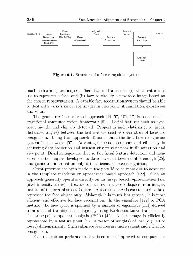
386 Face Detection, Alignment and Recognition Chapter 9
Face IDImage/VideoAligned
FaceFace
Location,Size & Pose
FeatureVectorFace
Detection------------------
Tracking
EnrolledUsers
FeatureMatching
FeatureExtraction
FaceAlignment
Figure 9.1. Structure of a face recognition system.
machine learning techniques. There two central issues: (i) what features touse to represent a face, and (ii) how to classify a new face image based onthe chosen representation. A capable face recognition system should be ableto deal with variations of face images in viewpoint, illumination, expressionand so on.
The geometric feature-based approach [44, 57, 101, 17] is based on thetraditional computer vision framework [81]. Facial features such as eyes,nose, mouth, and chin are detected. Properties and relations (e.g. areas,distances, angles) between the features are used as descriptors of faces forrecognition. Using this approach, Kanade built the first face recognitionsystem in the world [57]. Advantages include economy and efficiency inachieving data reduction and insensitivity to variations in illumination andviewpoint. Disadvantages are that so far, facial feature detection and mea-surement techniques developed to date have not been reliable enough [25],and geometric information only is insufficient for face recognition.
Great progress has been made in the past 15 or so years due to advancesin the template matching or appearance based approach [122]. Such anapproach generally operates directly on an image-based representation (i.e.pixel intensity array). It extracts features in a face subspace from images,instead of the over-abstract features. A face subspace is constructed to bestrepresent the face object only. Although it is much less general, it is moreefficient and effective for face recognition. In the eigenface [122] or PCAmethod, the face space is spanned by a number of eigenfaces [111] derivedfrom a set of training face images by using Karhunen-Loeve transform orthe principal component analysis (PCA) [42]. A face image is efficientlyrepresented by a feature point (i.e. a vector of weights) of low (e.g. 40 orlower) dimensionality. Such subspace features are more salient and richer forrecognition.
Face recognition performance has been much improved as compared to
Section 9.1. Introduction 387
that of the first automatic face recognition system of Kanade [57]. Nowadays,face detection, facial feature location, and recognition can be performed forimage data of reasonable conditions, which was un-achievable by the pioneersystems.
Although the progress has been encouraging, the task has also turnedout to be a very difficult endeavor [121]. Face recognition evaluation reportssuch as [95, 1] and other independent studies indicate that the performance ofmany state-of-the-art face recognition methods deteriorates with changes inlighting, pose, and other factors [123, 18, 140]. The key technical challengesare summarized in the following.Immense Variability of Facial Appearance. Whereas shape and re-flectance are intrinsic properties of a face object, the appearance (i.e. thetexture look) of a face is also subject to several other factors, including thefacial pose (or, equivalently, camera viewpoint), the illumination, facial ex-pression, and various imaging parameters such as aperture, exposure time,lens aberrations and sensor spectral response. All these factors are con-founded in the image data, so that “the variations between the images ofthe same face due to illumination and viewing direction are almost alwayslarger than the image variation due to change in face identity” [89]. Thecomplexity makes it very difficult to extract the intrinsic information of theface objects from their respective images.
Highly Complex and Nonlinear Manifolds. As illustrated above, theface manifold, as opposed to the manifold of non-face patterns, is highly non-convex, and so is face manifolds of any individual under changes due pose,lighting, facial ware and so on. As linear subspace method, such as princi-pal component analysis (PCA) [111, 122], independent component analysis(ICA) [10], or linear discriminant analysis (LDA) [12]) projects the data in ahigh dimensional space, such as the image space, to a low dimensional sub-space in an optimal direction in a linear way, they are unable to preserve thenon-convex variations of face manifolds necessary to differentiate betweendifferent individuals. In a linear subspace, Euclidean distance and more gen-erally M-distance, which are normally used in template matching, does notapply well to the problem of classification between manifolds of face/nonfacemanifolds and between manifolds of different individuals. This is a crucialfact that limits the power of the linear methods to achieve highly accurateface detection and recognition.
High Dimensionality and Small Sample Size. Another challenge isthe ability to generalize. A canonical face example used in face recognition
388 Face Detection, Alignment and Recognition Chapter 9
is an image of size 112 × 92 and resides in a 10304-dimensional real space.Nevertheless, the number of examples per person available for learning isusually much smaller than the dimensionality of the image space, e.g. < 10in most cases; a system trained on so few examples may not generalize wellto unseen face instances. Besides, the computational cost caused by highdimensionality is also a concern for real-time systems.
Methods for dealing with to the above problems are two ways. One isto normalize face images in geometry and photometry. This way, the facemanifolds become simpler, i.e. less nonlinear and less non-convex, so thatthe complex problems become easier to tackle. The other ways is to devisepowerful engines able to perform difficult nonlinear classification and regres-sion and generalize better. This relies on advances in pattern recognitionand learning and clever applications of them.
Both prior and observation constraints are needed for such powerful en-gines. Most successful approaches for tackling the above difficulties are basedon subspace modeling of facial appearance and statistical learning. Con-straints about the face include facial shape, texture, head pose, illuminationeffect. Recent advances allow these to be effectively encoded into the systemby learning from training data.
This chapter presents advanced techniques for face detection, face align-ment, and face recognition (feature extraction and matching). The presen-tation is focused on appearance and learning based approaches.
9.2 Face Detection
Face detection is the first step in automated face recognition. Its reliabilityhas a major influence on the performance and usability of the whole sys-tem. Given a single image or a video, an ideal face detection system shouldbe able to identify and locate all faces regardless of their positions, scales,orientations, lighting conditions, expressions, and so on.
Face detection can be performed based on several different cues: skincolor (for faces in color images), motion (for faces in videos), facial/headshape, and facial appearance, or a combination of them. Prior knowledgeabout them can be embedded into the system by learning from training data.
Appearance and learning based approaches have so far been the mosteffective ones for face detection, and this section focuses on such approachesfor face detection. The reader is referred to recent surveys [32, 136] for othermethods. Great resources such as publications, databases, codes, etc. canbe found from face detection websites [41, 133].

Section 9.2. Face Detection 389
9.2.1 Appearance and Learning Based Approach
In appearance based approach, face detection is treated as an intrinsicallytwo-dimensional (2-D) problem. It is done in three steps: First, scan Iexhaustively at all possible locations (u, v) and scales s, resulting in a largenumber of sub-windows x = x(u, v, s | I). Second, test for each x if it is aface
H(x)≥ 0 ⇒ x is a face pattern< 0 ⇒ x is a nonface pattern
(9.1)
Third, post-process to merge multiple detects.The key issue is the construction of a face detector which classifies a sub-
window into either face or nonface. Face and non-face examples are given asthe training set (See Fig. 9.2 for a random sample of 10 face and 10 nonfaceexamples). Taking advantage of the fact that faces are highly correlated, it isassumed that human faces can be described by some low dimensional featureswhich may be derived from a set of example face images. Large variationand complexity brought about by changes in facial appearance, lighting andexpression makes the face manifold highly complex [14, 110, 121]. Changes infacial view (head pose) further complicate the situation. Nonlinear classifiersare training to classify each subwindow into face or nonface. The followinggives a brief review of exiting work.
Figure 9.2. Face (top) and nonface (bottom) examples.
Turk and Pentland [122] describe a detection system based on a PrincipalComponent Analysis (PCA) subspace or eigenface representation. Moghad-dam and Pentland [87] present an improved method for Bayesian densityestimation, where the high dimensional image space is decomposed into aPCA subspace for prior distribution and the null space for the likelihooddistribution. Sung and Poggio [114] first partition the image space is intoseveral clusters for face and non-face clusters. Each cluster is then furtherdecomposed into the PCA and null subspaces. The Bayesian estimation isthen applied to obtain useful statistical features. Rowley et al. ’s system[100] uses retinally connected neural networks. Through a sliding window,the input images are examined after going through an extensive preprocess-

390 Face Detection, Alignment and Recognition Chapter 9
ing stage. Osuna et al. [91] train support vector machines to classify faceand non-face patterns. Roth et al. [99] use SNoW learning structure forface detection. In these systems, a bootstrap algorithm is used to iterativelycollect meaningful non-face examples into the training set.
Viola and Jones [128, 127] build a successful face detection system, inwhich AdaBoost learning is used to construct nonlinear classifier (earlierwork in application of Adaboost for image classification and face detectioncan be found in [117] and [104]). There, AdaBoost is adapted to solvingthe following three fundamental problems in one boosting procedure: (1)learning effective features from a large feature set, (2) constructing weakclassifiers each of which is based on one of the selected features, and (3)boosting the weak classifiers into a stronger classifier. Also, that work makesingenues use of several techniques for effective computation of a large numberof Haar wavelet like features. Such features are steerable filters [92, 128].Moreover, the simple-to-complex cascade of classifiers structure makes thecomputation even more efficient, which is in the principle of pattern rejection[8, 30] and coarse-to-fine search [5, 36]. Each such feature has a scalar valuewhich can be computed very efficiently [109] from the summed-area table[26] or integral image [128]. Their system is the first real-time frontal-viewface detector which runs at about 14 frame per second for a 320x240 image[128].
Ability to deal with non-frontal faces is important for many real appli-cations because statistics show that approximately 75% of the faces in homephotos are non-frontal [60]. A reasonable treatment for multi-view is theview-based method [93], in which several face models are built, each describ-ing faces in a certain view range. This way, explicit 3D modeling is avoided.Feraud et al. [34] adopt the view-based representation for face detection,and use an array of 5 detectors with each detector responsible for one view.Wiskott et al. [130] build elastic bunch graph templates for multi-view facedetection and recognition. Gong and colleagues [45] study the trajectoriesof faces in linear PCA feature spaces as they rotate, and use kernel supportvector machines (SVMs) for multi-pose face detection and pose estimation[90, 70]. Huang et al. [51] use SVM’s to estimate facial poses.
In the system of Schneiderman and Kanade [105], multi-resolution in-formation is used for different levels of wavelet transform. The algorithmconsists of an array of 5 face detectors in the view-based framework. Eachis constructed using statistics of products of histograms computed from ex-amples of the respective view. It takes 1 min for a 320x240 image over only4 octaves of candidate size according as reported in [105].
Li et al. [68, 67] present a multi-view face detection system, extending the
Section 9.2. Face Detection 391
work of [128, 127] and [105]. A new boosting algorithm called FloatBoost isproposed to incorporate Floating Search [97] into AdaBoost. The backtrackmechanism therein allows deletions of weak classifiers that are ineffective interms of the error rate, leading to a strong classifier consisting of fewer weakclassifiers. An extended Haar feature set is proposed for dealing with out-of-plane rotations and a detector pyramid for improving the speed. A coarse-to-fine, simple-to-complex architecture called detector-pyramid is designed forthe fast detection of multi-view faces. This work leads to the first real-timemulti-view face detection system in the world. It runs at 200 ms per imageof size 320x240 pixels on a Pentium-III CPU of 700 MHz.
Lienhart et al. [71] propose an extended set of rotated Haar featuresfor dealing with in-plane rotations. Also, they use Gentle Adaboost [37]with small CART trees as base classifiers and show that this combinationoutperforms that of Discrete Adaboost and stumps.
In the following, face processing techniques are presented, including pre-and post-processing, neural network based methods and boosting basedmethods. Given that the boosting learning with Haar-like feature approachhas achieved the best performance, the presentation will focus on such state-of-the-art methods.
9.2.2 Preprocessing
Skin Color Filtering
Human skin has its own distribution that differ from that of most of nonfaceobjects. It can be used to filtering the input image to obtain candidateregions of faces, and as a standalone face detector (not an appearance baseddetector). A simple color based face detection algorithm can consists of twosteps: (1) segmentation of likely face regions and (2) region merge.
Skin color likelihood model, p(color | face), can be derived from skincolor samples. This may be done in the H (of HSV) color space or in thenormalized RGB color space (cf. a comparative evaluation in [138]). AGaussian mixture model for p(color | face) can give a better skin colormodeling [132, 135]. Fig. 9.3 shows a skin color segmentation map. A skincolored pixel is found if p(H | face), where H is the hue component of thepixel, is greater than a threshold (0.3), and its saturation (S) and value(V) are between some upper and lower bounds. A skin color map consistsof a number of skin color regions which indicate potential candidate faceareas. Refined face regions can be obtained by merging adjacent similar andhomogeneous skin color pixels based on the color and spatial information.Heuristic postprocessing could be performed to remove false detection. For

392 Face Detection, Alignment and Recognition Chapter 9
example, a human face contains eyes where the eyes correspond to darkerregions inside the face region.
Figure 9.3. Skin color filtering: Input image with single (a) and multiple (c)people. Skin color filtered maps (b) and (d).
While a color based face detection system may work fast, however, thecolor constraint alone is insufficient for achieving high performance facedetection, due to color variations for different lighting, shadow, and ethicgroups. Indeed, it is the appearance, albeit colored or gray levelled, ratherthan the color that is essential for face detection. In fact, most successfulsystems need not use color and achieve good performance.
Image Normalization
Preprocessing operations are usually performed to normalize the image pat-tern in a subwindow in its size, pixel value distribution and lighting condi-tion. These include resizing (say, 20x20 pixels), lighting correction, meanvalue normalization, and histogram equalization. A simple lighting correc-tion operation is to subtract a best fit plane I ′(x, y) = a × x + b × y + cfrom the subwindow I(x, y), where the values of a, b and c can be estimatedusing the least squares method. Fig. 9.4 gives an example of the effect. Themean value normalization operation subtracts the mean value of the windowpattern from the window pixels so that the average intensity of all the pixelsin the subwindow is zero. See Fig. 9.5.
Multi-Gaussian Clustering
The distribution of training patterns is very complex because of the varietyof changes and high dimensionality. Therefore a single distribution is hard toexplain all such variations. Sung and Poggio [114] propose to deal with the
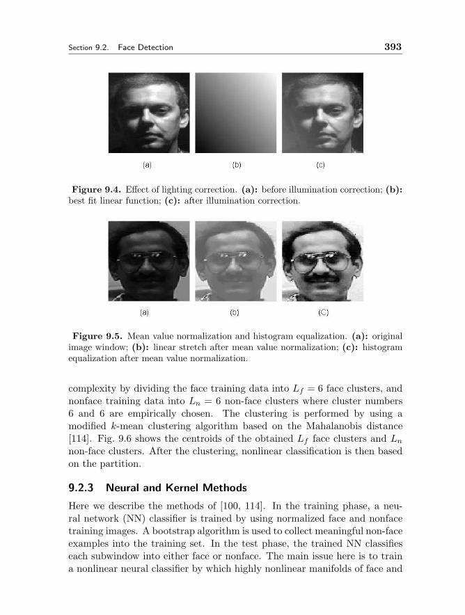
Section 9.2. Face Detection 393
Figure 9.4. Effect of lighting correction. (a): before illumination correction; (b):best fit linear function; (c): after illumination correction.
Figure 9.5. Mean value normalization and histogram equalization. (a): originalimage window; (b): linear stretch after mean value normalization; (c): histogramequalization after mean value normalization.
complexity by dividing the face training data into Lf = 6 face clusters, andnonface training data into Ln = 6 non-face clusters where cluster numbers6 and 6 are empirically chosen. The clustering is performed by using amodified k-mean clustering algorithm based on the Mahalanobis distance[114]. Fig. 9.6 shows the centroids of the obtained Lf face clusters and Lnnon-face clusters. After the clustering, nonlinear classification is then basedon the partition.
9.2.3 Neural and Kernel Methods
Here we describe the methods of [100, 114]. In the training phase, a neu-ral network (NN) classifier is trained by using normalized face and nonfacetraining images. A bootstrap algorithm is used to collect meaningful non-faceexamples into the training set. In the test phase, the trained NN classifieseach subwindow into either face or nonface. The main issue here is to traina nonlinear neural classifier by which highly nonlinear manifolds of face and
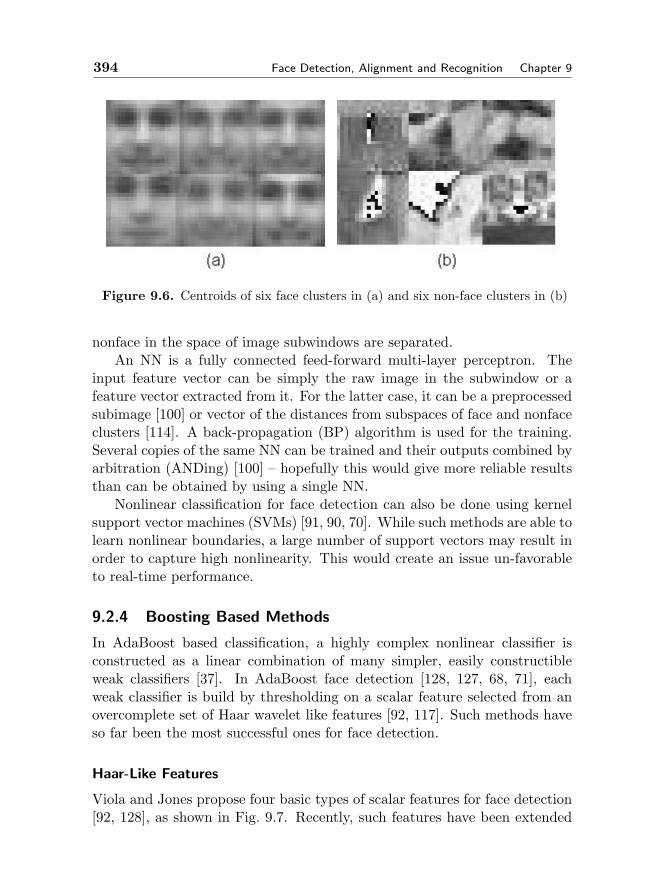
394 Face Detection, Alignment and Recognition Chapter 9
Figure 9.6. Centroids of six face clusters in (a) and six non-face clusters in (b)
nonface in the space of image subwindows are separated.An NN is a fully connected feed-forward multi-layer perceptron. The
input feature vector can be simply the raw image in the subwindow or afeature vector extracted from it. For the latter case, it can be a preprocessedsubimage [100] or vector of the distances from subspaces of face and nonfaceclusters [114]. A back-propagation (BP) algorithm is used for the training.Several copies of the same NN can be trained and their outputs combined byarbitration (ANDing) [100] – hopefully this would give more reliable resultsthan can be obtained by using a single NN.
Nonlinear classification for face detection can also be done using kernelsupport vector machines (SVMs) [91, 90, 70]. While such methods are able tolearn nonlinear boundaries, a large number of support vectors may result inorder to capture high nonlinearity. This would create an issue un-favorableto real-time performance.
9.2.4 Boosting Based Methods
In AdaBoost based classification, a highly complex nonlinear classifier isconstructed as a linear combination of many simpler, easily constructibleweak classifiers [37]. In AdaBoost face detection [128, 127, 68, 71], eachweak classifier is build by thresholding on a scalar feature selected from anovercomplete set of Haar wavelet like features [92, 117]. Such methods haveso far been the most successful ones for face detection.
Haar-Like Features
Viola and Jones propose four basic types of scalar features for face detection[92, 128], as shown in Fig. 9.7. Recently, such features have been extended
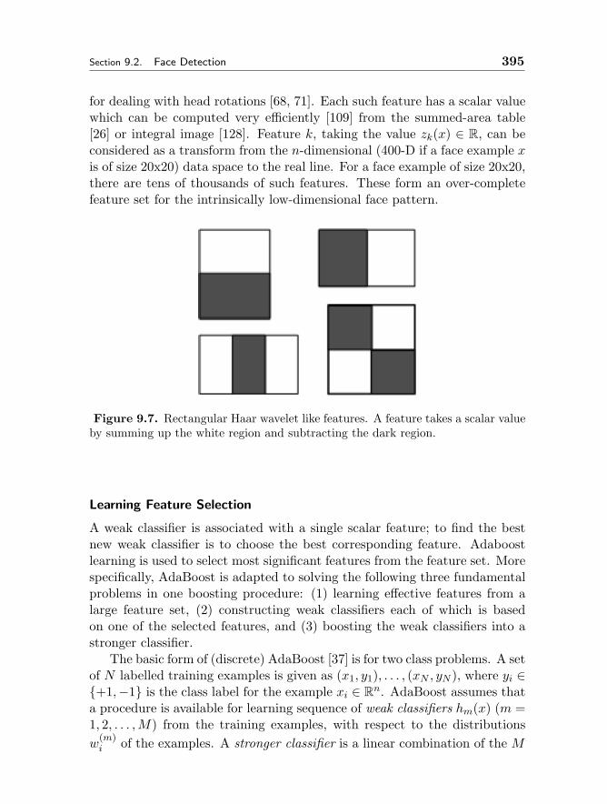
Section 9.2. Face Detection 395
for dealing with head rotations [68, 71]. Each such feature has a scalar valuewhich can be computed very efficiently [109] from the summed-area table[26] or integral image [128]. Feature k, taking the value zk(x) ∈ R, can beconsidered as a transform from the n-dimensional (400-D if a face example xis of size 20x20) data space to the real line. For a face example of size 20x20,there are tens of thousands of such features. These form an over-completefeature set for the intrinsically low-dimensional face pattern.
Figure 9.7. Rectangular Haar wavelet like features. A feature takes a scalar valueby summing up the white region and subtracting the dark region.
Learning Feature Selection
A weak classifier is associated with a single scalar feature; to find the bestnew weak classifier is to choose the best corresponding feature. Adaboostlearning is used to select most significant features from the feature set. Morespecifically, AdaBoost is adapted to solving the following three fundamentalproblems in one boosting procedure: (1) learning effective features from alarge feature set, (2) constructing weak classifiers each of which is basedon one of the selected features, and (3) boosting the weak classifiers into astronger classifier.
The basic form of (discrete) AdaBoost [37] is for two class problems. A setof N labelled training examples is given as (x1, y1), . . . , (xN , yN ), where yi ∈+1,−1 is the class label for the example xi ∈ R
n. AdaBoost assumes thata procedure is available for learning sequence of weak classifiers hm(x) (m =1, 2, . . . ,M) from the training examples, with respect to the distributionsw
(m)i of the examples. A stronger classifier is a linear combination of the M
396 Face Detection, Alignment and Recognition Chapter 9
weak classifiers
HM (x) =∑M
m=1 αmhm(x)∑Mm=1 αm
(9.2)
where αm ≥ 0 are the combining coefficients. The classification of x isobtained as y(x) = Sign[HM(x)] and the normalized confidence score is|HM (x)|. The AdaBoost learning procedure is aimed to derive αm andhm(x).
Learning Weak Classifiers
A weak classifier is constructed by thresholding one of those features accord-ing to the likelihoods (histograms) of the feature values for the target facesand the imposter faces
h(M)k (x) = +1 ifzk(x) > τ
(M)k (9.3)
= −1 otherwise (9.4)
where zk(x) is feature k extracted from x, and τ (M)k is the threshold for weak
classifier k chosen to ensure a specified accuracy. The best weak classifier isthe one for which the false alarm is minimized:
k∗ = arg minkFA(h(M)
k (x)) (9.5)
where FA is the false alarm caused by h(M)k (x) (also w.r.t. w(M−1)). This
gives us the best weak classifier as
hM (x) = h(M)k∗ (x) (9.6)
Boosted Strong Classifier
AdaBoost leans to boost weak classifiers hm into a strong one HM effectivelyby minimizing the upper bound on classification error achieved by HM . Thebound can be derived as the following exponential loss function [102]
J(HM ) =∑i
e−yiHM (xi) =∑i
e−yi∑M
m=1 αmhm(x) (9.7)
AdaBoost construct hm(x) by stagewise minimization of Eq.(9.7). Given thecurrent HM−1(x) =
∑M−1m=1 αmhm(x), and the newly learned weak classifier
hM , the best combining coefficient αM for the new strong classifier HM (x) =HM−1(x) + αMhM (x) minimizes the cost:
αM = arg minαJ(HM−1(x) + αhM (x)) (9.8)
Section 9.2. Face Detection 397
The minimizer is
αM = log1− εMεM
(9.9)
where εM is the weighted error
εM =∑i
w(M−1)i 1[sign(HM (xi)) = yi] (9.10)
where 1[C] is one if C is true, or 0 otherwise.Each example is re-weighted after an iteration, i.e. w
(M−1)i is updated
according to the classification performance of HM :
w(M)(x, y) = w(M−1)(x, y) exp (−αMyhM (x))= exp (−yHM (x)) (9.11)
which will be used for calculating the weighted error or another cost for train-ing the weak classifier in the next round. This way, a more difficult examplewill be associated with a larger weight so that it will be more emphasized inthe next round of learning. The algorithm is summarized in Fig. 9.8.
0.(Input)(1) Training examples Z = (x1, y1), . . . , (xN , yN ),
where N = a+ b; of which a examples have yi = +1and b examples have yi = −1;
(2) The number M of weak classifiers to be combined;1.(Initialization)
w(0)i = 1
2a for those examples with yi = +1 orw
(0)i = 1
2b for those examples with yi = −1.2.(Forward Inclusion)
For m = 1, . . . ,M :(1) Choose optimal hm to minimize weighted error;(2) Choose αm according to Eq.9.9;(3) Update w(m)
i ← w(m)i exp[−yihm(xi)], and
normalize to∑
i w(m)i = 1;
3.(Output)H(x) = sign[
∑Mm=1 hm(x)].
Figure 9.8. AdaBoost Learning Algorithm.
398 Face Detection, Alignment and Recognition Chapter 9
FloatBoost Learning
AdaBoost attempts to boost the accuracy of an ensemble of weak classifiersto a strong one. The AdaBoost algorithm [37] solved many of the practicaldifficulties of earlier boosting algorithms. Each weak classifier is trained onestage-wise to minimize the empirical error in a given distribution re-weightedaccording classification errors of the previously trained classifier. It is shownthat AdaBoost is a sequential forward search procedure using the greedyselection strategy to minimize a certain margin on the training set [102].
A crucial heuristic assumption made in such a sequential forward searchprocedure is the monotonicity, i.e. that when adding a new weak classifierto the current set, the value of the performance criterion does not decrease.The premise offered by the sequential procedure can be broken-down whenthe assumption is violated, i.e. when the performance criterion function isnon-monotonic. This is the first topic to be dealt with in this paper.
Floating Search [97] is a sequential feature selection procedure with back-tracking, aimed to deal with non-monotonic criterion functions for featureselection. A straight sequential selection method like sequential forwardsearch (SFS) or sequential backward search (SBS) adds or deletes one fea-ture at a time. To make this work well, the monotonicity property has tobe satisfied by the performance criterion function. Feature selection with anon-monotonic criterion may be dealt with by using a more sophisticatedtechnique, called plus--minus-r, which adds or deletes features and thenbacktracks r steps [113, 59].
The Sequential Floating Search methods [97] allows the number of back-tracking steps to be controlled instead of being fixed beforehand. Specifically,it adds or deletes = 1 feature and then backtracks r steps where r dependson the current situation. It is such a flexibility that amends limitationsdue to the non-monotonicity problem. Improvement on the quality of se-lected features is gained with the cost of increased computation due to theextended search. The SFFS algorithm performs very well in several applica-tions [97, 54]. The idea of Floating Search is further developed in [112] byallowing more flexibility for the determination of .
Let HM = h1, . . . , hM be the so-far-best set of M weak classifiers;J(HM ) be the criterion which measures the overall cost of the classifica-tion function HM (x) =
∑Mm=1 hm(x) build on HM ; Jmin
m be the minimumcost achieved so far with a linear combination of m weak classifiers form = 1, . . . ,Mmax (which are initially set to a large value before the iterationstarts). As shown in Fig. 9.9, the FloatBoost Learning procedure involvestraining inputs, initialization, forward inclusion, conditional exclusion and
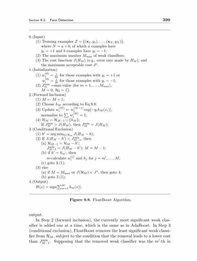
Section 9.2. Face Detection 399
0.(Input)(1) Training examples Z = (x1, y1), . . . , (xN , yN ),
where N = a+ b; of which a examples haveyi = +1 and b examples have yi = −1;
(2) The maximum number Mmax of weak classifiers;(3) The cost function J(HM ) (e.g., error rate made by HM ), and
the maximum acceptable cost J∗.1.(Initialization)
(1) w(0)i = 1
2a for those examples with yi = +1 orw
(0)i = 1
2b for those examples with yi = −1;(2) Jmin
m =max-value (for m = 1, . . . ,Mmax),M = 0, H0 = .
2.(Forward Inclusion)(1) M ←M + 1;(2) Choose hM according to Eq.9.8;(3) Update w(M)
i ← w(M−1)i exp[−yihM (xi)],
normalize to∑
i w(M)i = 1;
(4) HM = HM−1 ∪ hM;If Jmin
M > J(HM ), then JminM = J(HM );
3.(Conditional Exclusion)(1) h′ = arg minh∈HM
J(HM − h);(2) If J(HM − h′) < Jmin
M−1, then(a) HM−1 = HM − h′;
JminM−1 = J(HM − h′); M = M − 1;
(b) if h′ = hm′ , thenre-calculate w(j)
i and hj for j = m′, . . . ,M ;(c) goto 3.(1);
(3) else(a) if M = Mmax or J(HM ) < J∗, then goto 4;(b) goto 2.(1);
4.(Output)H(x) = sign[
∑Mm=1 hm(x)].
Figure 9.9. FloatBoost Algorithm.
output.In Step 2 (forward inclusion), the currently most significant weak clas-
sifier is added one at a time, which is the same as in AdaBoost. In Step 3(conditional exclusion), FloatBoost removes the least significant weak classi-fier from HM , subject to the condition that the removal leads to a lower costthan Jmin
M−1. Supposing that the removed weak classifier was the m′-th in
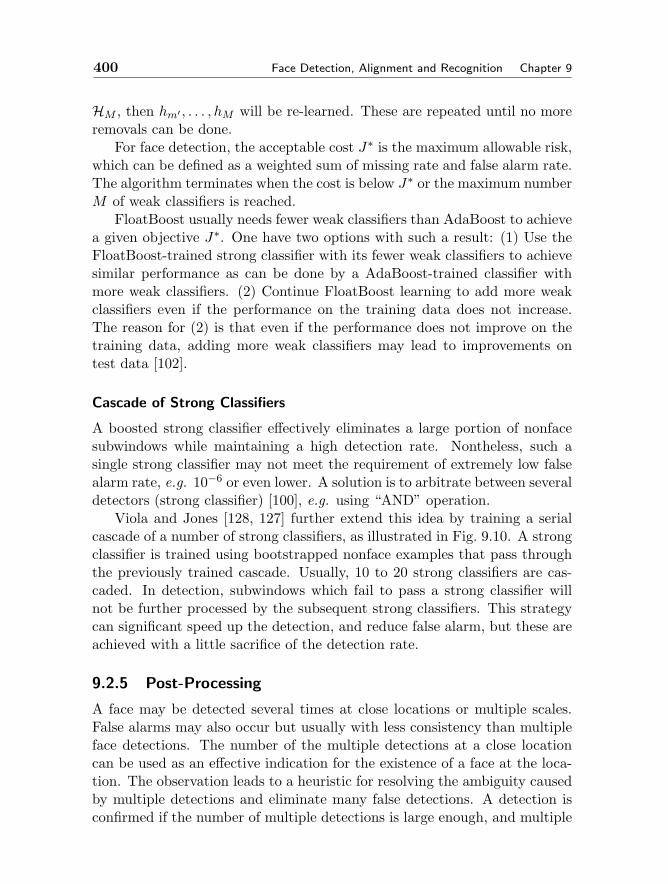
400 Face Detection, Alignment and Recognition Chapter 9
HM , then hm′ , . . . , hM will be re-learned. These are repeated until no moreremovals can be done.
For face detection, the acceptable cost J∗ is the maximum allowable risk,which can be defined as a weighted sum of missing rate and false alarm rate.The algorithm terminates when the cost is below J∗ or the maximum numberM of weak classifiers is reached.
FloatBoost usually needs fewer weak classifiers than AdaBoost to achievea given objective J∗. One have two options with such a result: (1) Use theFloatBoost-trained strong classifier with its fewer weak classifiers to achievesimilar performance as can be done by a AdaBoost-trained classifier withmore weak classifiers. (2) Continue FloatBoost learning to add more weakclassifiers even if the performance on the training data does not increase.The reason for (2) is that even if the performance does not improve on thetraining data, adding more weak classifiers may lead to improvements ontest data [102].
Cascade of Strong Classifiers
A boosted strong classifier effectively eliminates a large portion of nonfacesubwindows while maintaining a high detection rate. Nontheless, such asingle strong classifier may not meet the requirement of extremely low falsealarm rate, e.g. 10−6 or even lower. A solution is to arbitrate between severaldetectors (strong classifier) [100], e.g. using “AND” operation.
Viola and Jones [128, 127] further extend this idea by training a serialcascade of a number of strong classifiers, as illustrated in Fig. 9.10. A strongclassifier is trained using bootstrapped nonface examples that pass throughthe previously trained cascade. Usually, 10 to 20 strong classifiers are cas-caded. In detection, subwindows which fail to pass a strong classifier willnot be further processed by the subsequent strong classifiers. This strategycan significant speed up the detection, and reduce false alarm, but these areachieved with a little sacrifice of the detection rate.
9.2.5 Post-Processing
A face may be detected several times at close locations or multiple scales.False alarms may also occur but usually with less consistency than multipleface detections. The number of the multiple detections at a close locationcan be used as an effective indication for the existence of a face at the loca-tion. The observation leads to a heuristic for resolving the ambiguity causedby multiple detections and eliminate many false detections. A detection isconfirmed if the number of multiple detections is large enough, and multiple
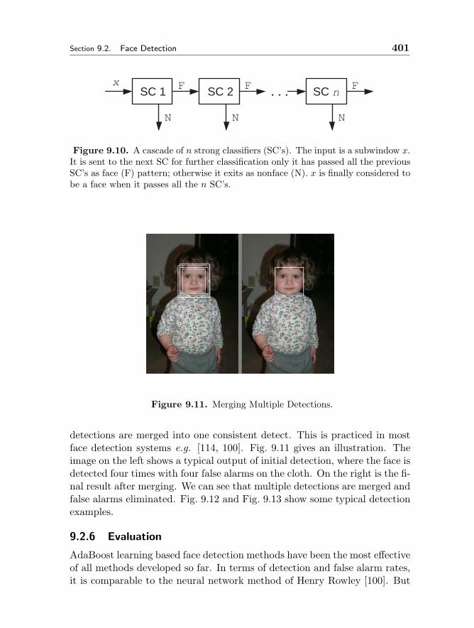
Section 9.2. Face Detection 401
SC 1 SC nSC 2
N NN
FF F...
x
Figure 9.10. A cascade of n strong classifiers (SC’s). The input is a subwindow x.It is sent to the next SC for further classification only it has passed all the previousSC’s as face (F) pattern; otherwise it exits as nonface (N). x is finally considered tobe a face when it passes all the n SC’s.
Figure 9.11. Merging Multiple Detections.
detections are merged into one consistent detect. This is practiced in mostface detection systems e.g. [114, 100]. Fig. 9.11 gives an illustration. Theimage on the left shows a typical output of initial detection, where the face isdetected four times with four false alarms on the cloth. On the right is the fi-nal result after merging. We can see that multiple detections are merged andfalse alarms eliminated. Fig. 9.12 and Fig. 9.13 show some typical detectionexamples.
9.2.6 Evaluation
AdaBoost learning based face detection methods have been the most effectiveof all methods developed so far. In terms of detection and false alarm rates,it is comparable to the neural network method of Henry Rowley [100]. But
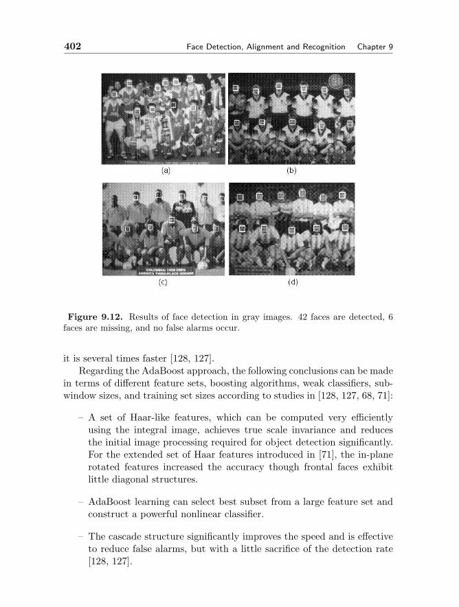
402 Face Detection, Alignment and Recognition Chapter 9
Figure 9.12. Results of face detection in gray images. 42 faces are detected, 6faces are missing, and no false alarms occur.
it is several times faster [128, 127].Regarding the AdaBoost approach, the following conclusions can be made
in terms of different feature sets, boosting algorithms, weak classifiers, sub-window sizes, and training set sizes according to studies in [128, 127, 68, 71]:
– A set of Haar-like features, which can be computed very efficientlyusing the integral image, achieves true scale invariance and reducesthe initial image processing required for object detection significantly.For the extended set of Haar features introduced in [71], the in-planerotated features increased the accuracy though frontal faces exhibitlittle diagonal structures.
– AdaBoost learning can select best subset from a large feature set andconstruct a powerful nonlinear classifier.
– The cascade structure significantly improves the speed and is effectiveto reduce false alarms, but with a little sacrifice of the detection rate[128, 127].
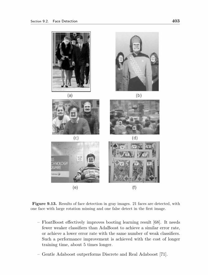
Section 9.2. Face Detection 403
Figure 9.13. Results of face detection in gray images. 21 faces are detected, withone face with large rotation missing and one false detect in the first image.
– FloatBoost effectively improves booting learning result [68]. It needsfewer weaker classifiers than AdaBoost to achieve a similar error rate,or achieve a lower error rate with the same number of weak classifiers.Such a performance improvement is achieved with the cost of longertraining time, about 5 times longer.
– Gentle Adaboost outperforms Discrete and Real Adaboost [71].
404 Face Detection, Alignment and Recognition Chapter 9
– It is beneficial not just to use the simplest of all tree classifiers, i.e.stumps, as the basis for the weak classifiers, but representationallymore powerful classifiers such as small CART trees, which can modelsecond and/or third order dependencies.
– 20x20 is the optimal input pattern size for frontal face detection.
Face detection technologies have now been mature enough to meet min-imum needs of many practical applications. However, much work is neededbefore automated face detection can achieve performance comparable withthe human. The Harr+AdaBoost approach is effective and efficient. How-ever, the current form has almost reached its power limit. Within sucha framework, possible improvements may be made by designing additionalnew set of features complement to the existing ones and adopting more ad-vanced learning techniques which could lead to classifiers which had complexenough boundaries yet did not overfit.
9.3 Face Alignment
Both shape and texture (i.e. image pixels enclosed in the facial outline)provide important clues useful for characterizing the face [13]. Accurate ex-traction of features for the representation of faces in images offers advantagesfor many applications, and is crucial for highly accurate face recognition andsynthesis. The task of face alignment is to accurately locate facial featuressuch as the eyes, nose, mouth and outline, and normalize facial shape andtexture.
Active Shape Model (ASM) [23] and Active Appearance Model (AAM)[22, 29] are two popular models for the purpose of shape and appearancemodeling and extraction. The standard ASM consists of two statisticalmodels: (1) global shape model, which is derived from the landmarks inthe object contour; (2) local appearance models, which is derived from theprofiles perpendicular to the object contour around each landmark. ASMuses local models to find the candidate shape and the global model to con-strain the searched shape. AAA makes use of subspace analysis techniques,PCA in particular, to model both shape variation and texture variation,and the correlations between them. In searching for a solution, it assumeslinear relationships between appearance variation and texture variation andbetween texture variation and position variation; and learns the two linearregression models from training data. The minimizations in high dimensionalspace is reduced in two models facilitate. This strategy is also developed inthe active blob model of Sclaroff and Isidoro [108].
Section 9.3. Face Alignment 405
ASM and AAM can be expanded in several ways. The concept, origi-nally proposed for the standard frontal view, can be extended to multi-viewfaces, either by using piecewise linear modeling [24] or nonlinear modeling[98]. Cootes and Taylor show that imposing constraints such as fixing eyelocations can improve AAM search result [21]. Blanz and Vetter extendedmorphable models and AAM to model relationship of 3D head geometryand facial appearance [16]. Li et al. [69] present a method for learning 3Dface shape model from 2D images based on a shape-and-pose-free texturemodel. In Duta et al. [28], the shapes are automatically aligned using pro-crustes analysis, and clustered to obtain cluster prototypes and statisticalinformation about intra-cluster shape variation. In Ginneken et al. [124],a K-nearest-neighbors classifier is used and a set of features are selectedfor each landmark to build local models. Baker and colleagues [7] proposean efficient method called “inverse compositional algorithm” for alignment.Ahlberg [4] extends AAM to a parametric method called Active Appearancealgorithm to extract positions parameterized by 3D rotation, 2D transla-tion, scale, and six Action Units (controlling the mouth and the eyebrows).In direct appearance model (DAM) [50, 66], shape is modeled as a linearfunction of texture. Using such an assumption, Yan et al. [131] proposetexture-constrained ASM (TC-ASM), which has the advantage of ASM inhaving good localization accuracy and that of AAM in having insensitivityto initialization.
The following describes ASM and AAM, DAM, TC-ASM. A trainingset of shape-texture pairs is assumed to be available and denoted as Ω =(S0, T0) where a shape S0 = ((x1, y1), . . . , (xK , yK)) ∈ R
2K is a sequenceof K points in the 2D image plane, and a texture T0 is the patch of pixelintensities enclosed by S0. Let S be the mean shape of all the trainingshapes, as illustrated in Fig. 9.14. All the shapes are aligned or warpingto the tangent space of the mean shape S. After that , the texture T0 iswarped correspondingly to T ∈ R
L, where L is the number of pixels in themean shape S. The warping may be done by pixel value interpolation, e.g.,using a triangulation or thin plate spline method.
9.3.1 Active Shape Model
In ASM, a shape is represented as a vector s in the low dimensional shapesubspace, denoted Ss, in R
k spanned by the k (< 2K) principal modeslearned from the training shapes.
S = S + Us (9.12)

406 Face Detection, Alignment and Recognition Chapter 9
Figure 9.14. Two face instaces labelled with 83 landmarks and the mesh of themean shape.
where U is the matrix consisting of k principal orthogonal modes of variationin S0. Because the training shapes have been aligned to the tangent spaceof S, the eigenvectors in U is orthogonal to the mean shape S, i.e., UTS = 0,and the projection from S to s is
s = UT (S − S) = UTS (9.13)
The local appearance models describing the typical images structurearound each landmark are obtained from the sampled profiles perpendic-ular to the landmark contour. The first derivatives of the profiles are usedto build these models. For a landmark, the mean profile and g and the co-variance matrix Sg can be computed from the example profiles directly. Thebest candidate can by found by minimizing Mahalanobis distance betweenthe candidate profile g and mean profile g:
dist(g, g) = (g − g)TS−1g (g − g) (9.14)
After relocating all the landmarks from local models, the result shape Sin the Ss can be derived from the likelihood distribution :
p(S|s) =exp−E(S|s)
Z(9.15)
where Z is the normalizing constant, and the corresponding likelihood energyfunction can be defined as:
E(S|s) =‖S − S′‖
2σ21
+k∑i=1
‖s′i − si‖22εi
(9.16)
where σ1 is a constant, εi is the i-th largest eigenvalue of the covariancematrix of the training data S0, S′ ∈ R
2K is the projection of S in Ss, ands′ is the corresponding shape parameters. The first term in Equ.(9.16) is the
Section 9.3. Face Alignment 407
Euclidean distance of S to the shape space Ss , and the second term is is theMahalanobis distance between s′ and s.
The maximum likelihood solution, sML = arg maxs∈Ss
p(S|s), is the projec-
tion of S to the shape space Ss, i.e.,
sML = UT (S − S) (9.17)
Its corresponding shape in R2K is
S = S + UsML (9.18)
9.3.2 Active Appearance Model
After aligning each training shape S0 to the mean shape and warping thecorresponding texture T0 to T , the warped textures are aligned to the tangentspace of the mean texture T by using an iterative approach [22]. The PCAmodel for the warped texture is obtained as
T = T + Vt (9.19)
where V is the matrix consisting of principal orthogonal modes of variationin T, t is the vector of texture parameters. The projection from T to t is
t = VT (T − T ) = VTT (9.20)
By this, the L pixel values in the mean shape is represented as a point inthe texture subspace St in R
.The appearance of each example is a concatenated vector
A =(
Λst
)(9.21)
where Λ is a diagonal matrix of weights for the shape parameters allowingfor the difference in units between the shape and texture variation, typicallydefined as rI. Again, by applying PCA on the set A, one gets
A = Wa (9.22)
where W is the matrix consisting of principal orthogonal modes of the vari-ation in A | for all training samples. The appearance subspace Sa is mod-elled by
a = WTA (9.23)
408 Face Detection, Alignment and Recognition Chapter 9
The search for an AAM solution is guided by the following differencebetween the texture Tim in the image patch and the texture Ta reconstructedfrom the current appearance parameters
δT = Tim − Ta (9.24)
More specifically, the search for a face in an image is guided by minimizingthe norm ‖δT‖. The AAM assumes that the appearance displacement δa andthe position (including coordinates (x, y), scale s, and rotation parameter θ)displacement δp are linearly correlated to δT :
δa = AaδT (9.25)δp = ApδT (9.26)
The prediction matrices Aa,Ap are to be learned from the training data byusing linear regression. In order to estimate Aa, a is displaced systematicallyto induce (δa, δT ) pairs for each training image. Due to large consumptionof memory required by the learning of Aa and Ap, the learning has to bedone with a small, limited set of δa, δT.
9.3.3 Modeling Shape from Texture
An analysis on mutual dependencies of shape, texture and appearance pa-rameters in the AAM subspace models shows that there exist admissibleappearances that are not modeled and hence cannot be reached by AAMsearch processing [50]. Let us look into relationship between shape and tex-ture from an intuitive viewpoint. A texture (i.e. the patch of intensities)is enclosed by a shape (before aligning to the mean shape); the same shapecan enclose different textures (i.e. configurations of pixel values). However,the reverse is not true: different shapes can not enclose the same texture. Sothe mapping from the texture space to the shape space is many-to-one. Theshape parameters should be determined completely by texture parametersbut not vice versa.
Then, let us look further into the correlations or constraints between thelinear subspaces Ss,St and Sa in terms of their dimensionalities or ranks. Letdenote the rank of space S by dim(S). The following analysis is made in [50]:
1. When dim(Sa)=dim(St)+dim(Ss), the shape and texture parametersare independent of each other, and there exist no mutual constraintsbetween the parameters s and t.
2. When dim(St)<dim(Sa)<dim(St)+dim(Ss), not all the shape param-eters are independent of the texture parameters. That is, one shape
Section 9.3. Face Alignment 409
can correspond to more than one texture configuration in it, whichconforms an intuition.
3. One can also derive the relationship dim(St)<dim(Sa) from Eq.(9.21)and (9.22) the formula
Wa =(
Λst
)(9.27)
when that s contains some components which are independent of t.
4. However, in AAM, it is often the case where dim(Sa)<dim(St) if thedimensionalities of Sa and St are chosen to retain, say 98%, of thetotal variations [22]. The consequence is that some admissible textureconfigurations cannot been seen in the appearance subspace becausedim(Sa)<dim(St), and therefore cannot be reached by the AAM search.This a flaw of AAM’s modeling of its appearance subspace.
From the above analysis, It is concluded in [50] that the ideal modelshould be such that dim(Sa)=dim(St) and hence that s completely linearlydeterminable by t. In other words, the shape should be linearly dependenton the texture so that dim(St ∪ Ss)=dim(St).
Direct Appearance Models
A solution to this problem is made by assuming that the shape is linearlydependent on the texture [50, 66]:
s = Rt+ ε (9.28)
where ε = s − Rt is noise and R is a k × l projection matrix. Denotingthe expectation by E(·), if all the elements in the variance matrix E(εεT )are small enough, the linear assumption made in Eq.(9.28) is approximatelycorrect. This is true as will be verified later by experiments. Define theobjective cost function
C(R) = E(εT ε) = trace[E(εεT )] (9.29)
R is learned from training example pairs (s, t) by minimizing the abovecost function. The the optimal solution is
R∗ = E(stT )[E(ttT )]−1 (9.30)
The minimized cost is the trace of the following
E(εεT ) = E(ssT )−R∗E(ttT )R∗T (9.31)
410 Face Detection, Alignment and Recognition Chapter 9
DAM [50, 66] assumes that the facial shape is a linear regression func-tion of the facial texture and hence overcomes a defect in AAM; the textureinformation is used directly to predict the shape and to update the estimatesof position and appearance (hence the name DAM). Also, DAM predictsthe new face position and appearance based on the principal components oftexture difference vectors, instead of the raw vectors themselves as in AAM.This cuts down the memory requirement to a large extent, and further im-proves the convergence rate and accuracy.
Learning in DAM
The DAM consists of a shape model, two texture (original and residual)model and two prediction (position and shape prediction) model. The shape,texture models and the position prediction model (9.26) are built in thesame way as in AAM. The residual texture model is built using the subspaceanalysis technique PCA. Abandoning AAM’s crucial idea of combining shapeand texture parameters into an appearance model, it predicts the shapeparameters directly from the texture parameters. In the following, the lasttwo models are demonstrated in detail.
Instead of using δT directly as in the AAM search (cf. Eq.(9.26), itsprincipal components, denoted δT ′, is used to predict the position displace-ment
δp = RpδT′ (9.32)
where Rp is the prediction matrix learned by using linear regression. Todo this, samples of texture differences induced by small position displace-ments in each training image are collected, and PCA is performed to get theprojection matrix HT . A texture difference is projected onto this subspaceas
δT ′ = HT δT (9.33)
δT ′ is normally about 1/4 of δT in dimensionality. Results have shown thatthe use of δT instead of δT ′ as in Eq.(9.32) makes the prediction more stableand more accurate.
Assume that a training set be given as A = (Si, T oi ) where a shapeSi = ((xi1, y
i1), . . . , (x
iK , y
iK)) ∈ R
2K is a sequence of K points in the 2D im-age plane, and a texture T oi is the patch of image pixels enclosed by Si. TheDAM learning consists of two parts: (1) learning R, and (2) learning H andRp: (1) R is learned from the shape-texture pairs s, t obtained from thelandmarked images. (2) To learn H and Rp, artificial training data is gener-ated by perturbing the position parameters p around the landmark points to
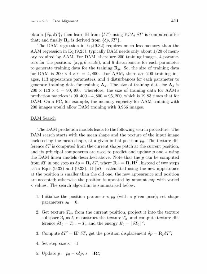
Section 9.3. Face Alignment 411
obtain δp, δT; then learn H from δT using PCA; δT ′ is computed afterthat; and finally Rp is derived from δp, δT ′.
The DAM regression in Eq.(9.32) requires much less memory than theAAM regression in Eq.(9.25), typically DAM needs only about 1/20 of mem-ory required by AAM. For DAM, there are 200 training images, 4 parame-ters for the position: (x, y, θ, scale), and 6 disturbances for each parameterto generate training data for the training Rp. So, the size of training datafor DAM is 200 × 4 × 6 = 4, 800. For AAM, there are 200 training im-ages, 113 appearance parameters, and 4 disturbances for each parameter togenerate training data for training Aa. The size of training data for Aa is200 × 113 × 4 = 90, 400. Therefore, the size of training data for AAM’sprediction matrices is 90, 400+4, 800 = 95, 200, which is 19.83 times that forDAM. On a PC, for example, the memory capacity for AAM training with200 images would allow DAM training with 3,966 images.
DAM Search
The DAM prediction models leads to the following search procedure: TheDAM search starts with the mean shape and the texture of the input imageenclosed by the mean shape, at a given initial position p0. The texture dif-ference δT is computed from the current shape patch at the current position,and its principal components are used to predict and update p and s usingthe DAM linear models described above. Note that the p can be computedfrom δT in one step as δp = RT δT , where RT = RpHT , instead of two stepsas in Eqns.(9.32) and (9.33). If ‖δT‖ calculated using the new appearanceat the position is smaller than the old one, the new appearance and positionare accepted; otherwise the position is updated by amount κδp with variedκ values. The search algorithm is summarized below:
1. Initialize the position parameters p0 (with a given pose); set shapeparameters s0 = 0;
2. Get texture Tim from the current position, project it into the texturesubspace St as t, reconstruct the texture Ta, and compute texture dif-ference δT0 = Tim − Ta and the energy E0 = ‖δT0‖2;
3. Compute δT ′ = HT δT , get the position displacement δp = RpδT′;
4. Set step size κ = 1;
5. Update p = p0 − κδp, s = Rt;
412 Face Detection, Alignment and Recognition Chapter 9
6. Compute the difference texture δT using the new shape at the newposition, and its energy E = ‖δT‖2;
7. If |E − E0| < ε, the algorithm is converged; exit;
8. If E < E0, then let p0 = p, s0 = s, δT0 = δT,E0 = E, goto 3;
9. Change κ to the next number in 1.5, 0.5, 0.25, 0.125, . . . , , goto 5;
Texture-Constrained Active Shape Model
TC-ASM [131] imposes the linear relationship of direct appearance model(DAM) to improve ASM search. The motivation is the following: ASM hasbetter accuracy in shape localization than AAM when the initial shape isplaced close enough to the true shape whereas the latter model incorporatesinformation about texture enclosed in the shape and hence yields lower tex-ture reconstruction error. However, ASM makes use of constraints near theshape only, without a global optimality criterion, and therefore the solutionis sensitive to the initial shape position. In AAM, the solution finding pro-cess is based on the linear relationship between the variation of the positionand the texture reconstruct error. The reconstruct error δT is influencedvery much by the illumination. Since δT is orthogonal to St (projected backto R
L) and dim(St) dim(T ), the dimension of the space δT is very high,and it is hard to train the regression matrix Aa,Ap and the prediction of thevariance of position can be subject to significant errors. Also it is time andmemory consuming. TC-ASM is aimed to overcome the above problems.
TC-ASM consists of a shape model, a global texture model, K localappearance (likelihood) models and a texture-shape model. The shape andtexture model are built based on PCA in the way as in AAM. TheK local ap-pearance models are build from the sampled profiles around each landmark,and the texture-shape model is learned from the pairs (s,t) obtained fromthe landmarked images.
It assumes a linear relationship between shape and texture as in DAM.The shape (∈ Ss) with a given texture (∈ St) can be approximately modelledby Gaussian distribution:
s ∼ N(st,Λ′) (9.34)
wherest = Rt+ ε (9.35)
where ε is the noise, and Λ′ can be defined as diagonal matrix for simplicity.The matrix R can be pre-computed from the training pairs (s,t) ob-
tained from the labelled images using the Least Square method. The matrix
Section 9.3. Face Alignment 413
R will map the texture to the mean shape of all shapes with the same tex-ture, i.e., E(s| shape S with parameter s encloses the given texture t), andit’s right to be the expectation of the distribution, i.e., st. Denoting:
RV T = RV T (9.36)
From Equ.(9.20) and Equ.(9.35), one can get
st = RV T (T − T ) (9.37)
Then the prior conditional distribution of s ∈ Ss, for a given st can berepresented as:
p(s|st) =exp−E(s|st)
Z ′ (9.38)
where Z ′ is the normalizing constant and the corresponding energy functionis:
E(s|st) =k∑i=1
‖si − sti‖22ε′i
(9.39)
TC-ASM search is formulated in the Bayesian framework. Intuitively,one could assume ε′ = βε or ε′ = σ2I, where ε = (ε1, ..., εk)T is the klargest eigenvalues of the covariance matrix of the training data S0 and βis a constant. Using the prior distribution of Equ.(9.38) and the likelihooddistribution in Equ.(9.16).
Let S be the shape derived from local appearance models, and st bethe predicted shape from the global texture constrains. S and st can beconsidered to be independent each other, i.e.,
p(S, st) = p(S)p(st) and p(S|st) = p(S) (9.40)
Shape extraction is posed as a problem of maximum a posterior (MAP)estimation. The posteriori distribution of s ∈ Ss is:
p(s|S, st) =p(S|s, st)p(s, st)
p(S, st)(9.41)
=p(S|s)p(s|st)
p(S)(9.42)
The corresponding energy is
E(s|S, st) = E(S|s) + E(s|st) (9.43)
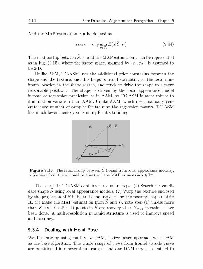
414 Face Detection, Alignment and Recognition Chapter 9
And the MAP estimation can be defined as
sMAP = argmins∈Ss
E(s|S, st) (9.44)
The relationship between S, st and the MAP estimation s can be representedas in Fig. (9.15), where the shape space, spanned by e1, e2, is assumed tobe 2-D.
Unlike ASM, TC-ASM uses the additional prior constrains between theshape and the texture, and this helps to avoid stagnating at the local min-imum location in the shape search, and tends to drive the shape to a morereasonable position. The shape is driven by the local appearance modelinstead of regression prediction as in AAM, so TC-ASM is more robust toillumination variation than AAM. Unlike AAM, which need manually gen-erate huge number of samples for training the regression matrix, TC-ASMhas much lower memory consuming for it’s training.
Figure 9.15. The relationship between S (found from local appearance models),st (derived from the enclosed texture) and the MAP estimation s ∈ R
k.
The search in TC-ASM contains three main steps: (1) Search the candi-date shape S using local appearance models, (2) Warp the texture enclosedby the projection of S in Ss and compute st using the texture-shape matrixR, (3) Make the MAP estimation from S and st, goto step (1) unless morethan K ∗ θ( 0 < θ < 1) points in S are converged or Nmax iterations havebeen done. A multi-resolution pyramid structure is used to improve speedand accuracy.
9.3.4 Dealing with Head Pose
We illustrate by using multi-view DAM, a view-based approach with DAMas the base algorithm. The whole range of views from frontal to side viewsare partitioned into several sub-ranges, and one DAM model is trained to
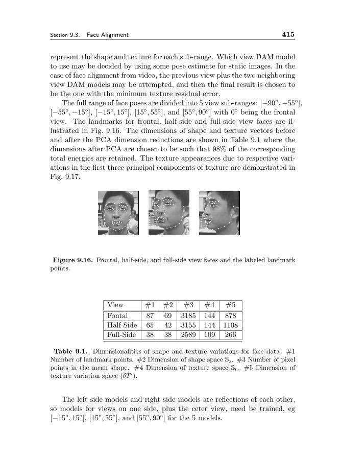
Section 9.3. Face Alignment 415
represent the shape and texture for each sub-range. Which view DAM modelto use may be decided by using some pose estimate for static images. In thecase of face alignment from video, the previous view plus the two neighboringview DAM models may be attempted, and then the final result is chosen tobe the one with the minimum texture residual error.
The full range of face poses are divided into 5 view sub-ranges: [−90,−55],[−55,−15], [−15, 15], [15, 55], and [55, 90] with 0 being the frontalview. The landmarks for frontal, half-side and full-side view faces are il-lustrated in Fig. 9.16. The dimensions of shape and texture vectors beforeand after the PCA dimension reductions are shown in Table 9.1 where thedimensions after PCA are chosen to be such that 98% of the correspondingtotal energies are retained. The texture appearances due to respective vari-ations in the first three principal components of texture are demonstrated inFig. 9.17.
Figure 9.16. Frontal, half-side, and full-side view faces and the labeled landmarkpoints.
View #1 #2 #3 #4 #5Fontal 87 69 3185 144 878Half-Side 65 42 3155 144 1108Full-Side 38 38 2589 109 266
Table 9.1. Dimensionalities of shape and texture variations for face data. #1Number of landmark points. #2 Dimension of shape space Ss. #3 Number of pixelpoints in the mean shape. #4 Dimension of texture space St. #5 Dimension oftexture variation space (δT ′).
The left side models and right side models are reflections of each other,so models for views on one side, plus the ceter view, need be trained, eg[−15, 15], [15, 55], and [55, 90] for the 5 models.
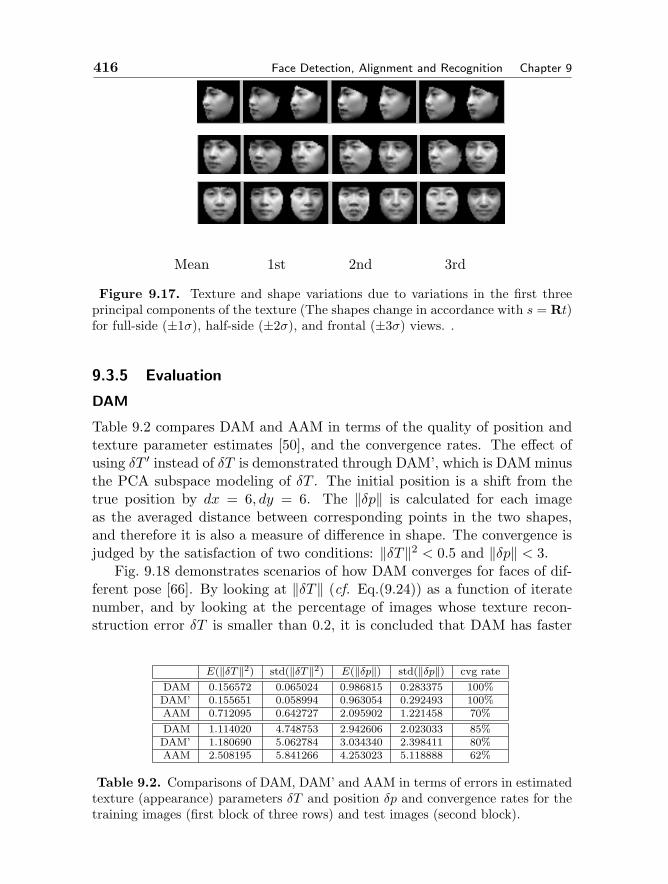
416 Face Detection, Alignment and Recognition Chapter 9
Mean 1st 2nd 3rd
Figure 9.17. Texture and shape variations due to variations in the first threeprincipal components of the texture (The shapes change in accordance with s = Rt)for full-side (±1σ), half-side (±2σ), and frontal (±3σ) views. .
9.3.5 Evaluation
DAM
Table 9.2 compares DAM and AAM in terms of the quality of position andtexture parameter estimates [50], and the convergence rates. The effect ofusing δT ′ instead of δT is demonstrated through DAM’, which is DAM minusthe PCA subspace modeling of δT . The initial position is a shift from thetrue position by dx = 6, dy = 6. The ‖δp‖ is calculated for each imageas the averaged distance between corresponding points in the two shapes,and therefore it is also a measure of difference in shape. The convergence isjudged by the satisfaction of two conditions: ‖δT‖2 < 0.5 and ‖δp‖ < 3.
Fig. 9.18 demonstrates scenarios of how DAM converges for faces of dif-ferent pose [66]. By looking at ‖δT‖ (cf. Eq.(9.24)) as a function of iteratenumber, and by looking at the percentage of images whose texture recon-struction error δT is smaller than 0.2, it is concluded that DAM has faster
E(‖δT‖2) std(‖δT‖2) E(‖δp‖) std(‖δp‖) cvg rateDAM 0.156572 0.065024 0.986815 0.283375 100%DAM’ 0.155651 0.058994 0.963054 0.292493 100%AAM 0.712095 0.642727 2.095902 1.221458 70%DAM 1.114020 4.748753 2.942606 2.023033 85%DAM’ 1.180690 5.062784 3.034340 2.398411 80%AAM 2.508195 5.841266 4.253023 5.118888 62%
Table 9.2. Comparisons of DAM, DAM’ and AAM in terms of errors in estimatedtexture (appearance) parameters δT and position δp and convergence rates for thetraining images (first block of three rows) and test images (second block).
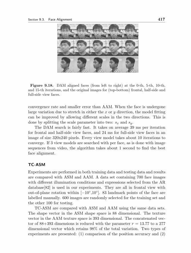
Section 9.3. Face Alignment 417
Figure 9.18. DAM aligned faces (from left to right) at the 0-th, 5-th, 10-th,and 15-th iterations, and the original images for (top-bottom) frontal, half-side andfull-side view faces.
convergence rate and smaller error than AAM. When the face is undergonelarge variation due to stretch in either the x or y direction, the model fittingcan be improved by allowing different scales in the two directions. This isdone by splitting the scale parameter into two: sx and sy.
The DAM search is fairly fast. It takes on average 39 ms per iterationfor frontal and half-side view faces, and 24 ms for full-side view faces in animage of size 320x240 pixels. Every view model takes about 10 iterations toconverge. If 3 view models are searched with per face, as is done with imagesequences from video, the algorithm takes about 1 second to find the bestface alignment.
TC-ASM
Experiments are performed in both training data and testing data and resultsare compared with ASM and AAM. A data set containing 700 face imageswith different illumination conditions and expressions selected from the ARdatabase[82] is used in our experiments. They are all in frontal view without-of-plane rotation within [−10,10]. 83 landmark points of the face arelabelled manually. 600 images are randomly selected for the training set andthe other 100 for testing.
TC-ASM are compared with ASM and AAM using the same data sets.The shape vector in the ASM shape space is 88 dimensional. The texturevector in the AAM texture space is 393 dimensional. The concatenated vec-tor of 88+393 dimensions is reduced with the parameter r = 13.77 to a 277dimensional vector which retains 98% of the total variation. Two types ofexperiments are presented: (1) comparison of the position accuracy and (2)
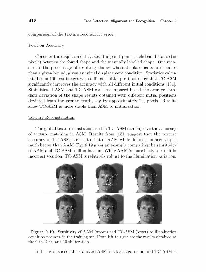
418 Face Detection, Alignment and Recognition Chapter 9
comparison of the texture reconstruct error.
Position Accuracy
Consider the displacement D, i.e., the point-point Euclidean distance (inpixels) between the found shape and the manually labelled shape. One mea-sure is the percentage of resulting shapes whose displacements are smallerthan a given bound, given an initial displacement condition. Statistics calcu-lated from 100 test images with different initial positions show that TC-ASMsignificantly improves the accuracy with all different initial conditions [131].Stabilities of ASM and TC-ASM can be compared based the average stan-dard deviation of the shape results obtained with different initial positionsdeviated from the ground truth, say by approximately 20, pixels. Resultsshow TC-ASM is more stable than ASM to initialization.
Texture Reconstruction
The global texture constrains used in TC-ASM can improve the accuracyof texture matching in ASM. Results from [131] suggest that the textureaccuracy of TC-ASM is close to that of AAM while its position accuracy ismuch better than AAM. Fig. 9.19 gives an example comparing the sensitivityof AAM and TC-ASM to illumination. While AAM is more likely to result inincorrect solution, TC-ASM is relatively robust to the illumination variation.
Figure 9.19. Sensitivity of AAM (upper) and TC-ASM (lower) to illuminationcondition not seen in the training set. From left to right are the results obtained atthe 0-th, 2-th, and 10-th iterations.
In terms of speed, the standard ASM is a fast algorithm, and TC-ASM is

Section 9.4. Face Recognition 419
computationally more expensive but still much faster than AAM. The train-ing of TC-ASM is very fast, which takes only about one tenth of AAM. Inour experiment (600 training images, 83 landmarks and P-III 700 computer),TC-ASM takes on average 32 ms per iteration, which is twice of ASM (16ms), while only one fifth of AAM(172 ms). The training time of AAM ismore than two hours, while TC-ASM is only about 12 minutes.
9.4 Face Recognition
To date, the appearance-based learning framework has been most influentialin the face recognition (FR) research. Under this framework, the FR problemcan be stated as follows: Given a training set, Z = ZiCi=1, containing Cclasses with each class Zi = zijCi
j=1 consisting of a number of localized face
images zij , a total of N =∑C
i=1Ci face images are available in the set. Forcomputational convenience, each image is represented as a column vectorof length J(= Iw × Ih) by lexicographic ordering of the pixel elements, i.e.zij ∈ R
J , where (Iw×Ih) is the image size, and RJ denotes the J-dimensional
real space. Taking as input such a set Z, the objectives of appearance-based learning are: (1) to find based on optimization of certain separabilitycriteria a low-dimensional feature representation yij = ϕ(zij), yij ∈ R
M andM J , with enhanced discriminatory power; (2) to design based on thechosen representation a classifier, h : R
M → Y = 1, 2, · · · , C, such that hwill correctly classify unseen examples ϕ(z, y), where y ∈ Y is the class labelof z.
9.4.1 Preprocessing
Figure 9.20. Left: Original samples in the FERET database [3]. Middle: Thestandard mask. Right: The samples after the preprocessing sequence.
It has been shown that irrelevant facial portions such as hair, neck, shoul-der and background often provide misleading information to the FR systems[20]. A normalization procedure is recommended in [95], using geometriclocations of facial features found in face detection and alignment. The nor-
420 Face Detection, Alignment and Recognition Chapter 9
malization sequence consists of four steps: (1) the raw images are translated,rotated and scaled so that the centers of the eyes are placed on specific pix-els, (2) a standard mask as shown in Fig. 9.20:Middle is applied to removethe non-face portions, (3) histogram equalization is performed in the nonmasked facial pixels, (4) face data are further normalized to have zero meanand unit standard deviation. Fig. 9.20:Right depicts some samples obtainedafter the preprocessing sequence was applied.
9.4.2 Feature Extraction
The goal of feature extraction is to generate a low-dimensional feature repre-sentation intrinsic to face objects with good discriminatory power for patternclassification.
PCA Subspace
In the statistical pattern recognition literature, Principle Component Anal-ysis (PCA) [55] is one of the most widely used tools for data reduction andfeature extraction. The well-known FR method, Eigenfaces [122] built onthe PCA technique, has been proved to be very successful. In the Eigen-faces method [122], the PCA is applied to the training set Z to find the Neigenvectors (with non zero eigenvalues) of the set’s covariance matrix,
Scov =1N
C∑i=1
Ci∑j=1
(zij − z)(zij − z)T (9.45)
where z = 1N
∑Ci=1∑Ci
j=1 zij is the average of the ensemble. The Eigen-faces are the first M(≤ N) eigenvectors (denoted as Ψef ) corresponding tothe largest eigenvalues, and they form a low-dimensional subspace, called“face space” where most energies of the face manifold are supposed to lie.Fig. 9.21(1st row) shows the first 6 Eigenfaces, which appear as some re-searchers said ghostly faces. Transforming to the M -dimensional face spaceis a simple linear mapping: yij = ΨT
ef (zij − z), where the basis vectorsΨef are orthonormal. The subsequent classification of face patterns can beperformed in the face space using any classifier.
Dual PCA Subspaces
The Eigenfaces method is built on a single PCA, which suffers from a majordrawback, that is, it can not explicitly account for the difference betweentwo types of face pattern variations key to the FR task: between-class vari-ations and within-class variations. To this end, Moghaddam et al. [86]
Section 9.4. Face Recognition 421
proposed a probabilistic subspace method, also known as dual Eigenfaces.In the method, the distribution of face pattern is modelled by the intensitydifference between two face images, ∆ = z1 − z2. The difference ∆ canbe contributed by two distinct and mutually exclusive classes of variations:intrapersonal variations ΩI and extrapersonal variations ΩE . In this way,the C-class FR task is translated to a binary pattern classification problem.Each class of variations can be modelled by a high-dimensional Gaussiandistribution, P (∆|Ω). Since most energies of the distribution are assumedto exist in a low-dimensional PCA subspace, it is shown in [86] that P (∆|Ω)can be approximately estimated by
P (∆|Ω) = P (z1 − z2|Ω) = exp(−‖y1 − y2‖2 /2)/β(Ω) (9.46)
where y1 and y2 are the projections of z1 and z2 in the PCA subspace, andβ(Ω) is a normalization constant for a given Ω. Any two images can bedetermined if come from the same person by comparing the two likelihoods,P (∆|ΩI) and P (∆|ΩE), based on the maximum-likelihood (ML) classifica-tion rule. It is commonly believed that the extrapersonal PCA subspace asshown in Fig. 9.21(2nd row) represents more representative variations, suchas those captured by the standard Eigenfaces method whereas the intraper-sonal PCA subspace shown in Fig. 9.21(3rd row) accounts for variations duemostly to changes in expression. Also, it is not difficult to see that the twoGaussian covariance matrices in P (∆|ΩI) and P (∆|ΩE) are equivalent to thewithin- and between-class scatter matrices of Linear Discriminant Analysis(LDA) mentioned later respectively. Thus, the dual Eigenfaces method canbe regarded as a quadratic extension of the so-called Fisherfaces method [12].
Other PCA Extensions
The PCA-based methods are simple in theory, but they started the era ofthe appearance-based approach to visual object recognition [121]. In addi-tion to the dual Eigenfaces method, numerous extensions or variants of theEigenfaces method have been developed for almost every area of face re-search. For example, a multiple-observer Eigenfaces technique is presentedto deal with view-based face recognition in [93]. Moghaddam and Pentlandderived two distance metrics, called distance from face space (DFFS) anddistance in face space (DIFS), by performing density estimation in the origi-nal image space using Gaussian models, for visual object representation [87].Sung and Poggio built six face spaces and six non-face spaces, extracted theDEFS and DIFS of the input query image in each face/non-face space, andthen fed them to a multi-layer perceptron for face detection [114]. Tipping
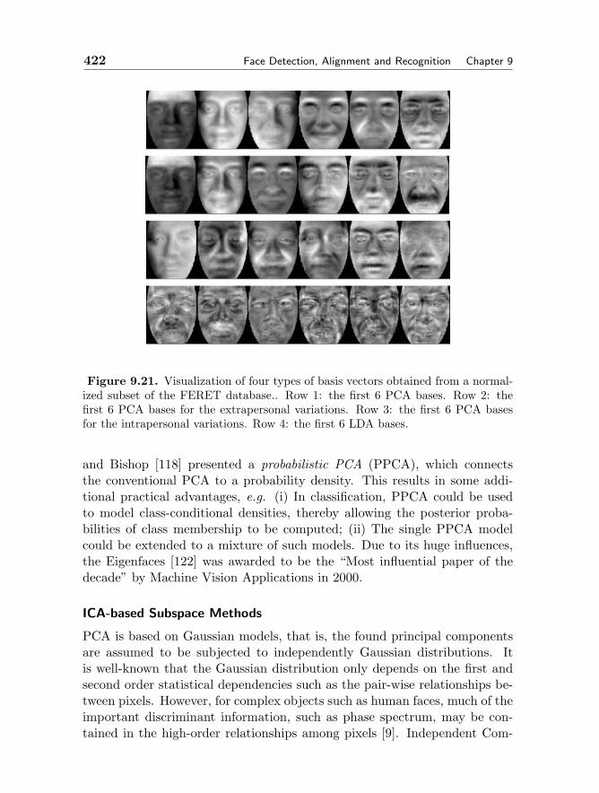
422 Face Detection, Alignment and Recognition Chapter 9
Figure 9.21. Visualization of four types of basis vectors obtained from a normal-ized subset of the FERET database.. Row 1: the first 6 PCA bases. Row 2: thefirst 6 PCA bases for the extrapersonal variations. Row 3: the first 6 PCA basesfor the intrapersonal variations. Row 4: the first 6 LDA bases.
and Bishop [118] presented a probabilistic PCA (PPCA), which connectsthe conventional PCA to a probability density. This results in some addi-tional practical advantages, e.g. (i) In classification, PPCA could be usedto model class-conditional densities, thereby allowing the posterior proba-bilities of class membership to be computed; (ii) The single PPCA modelcould be extended to a mixture of such models. Due to its huge influences,the Eigenfaces [122] was awarded to be the “Most influential paper of thedecade” by Machine Vision Applications in 2000.
ICA-based Subspace Methods
PCA is based on Gaussian models, that is, the found principal componentsare assumed to be subjected to independently Gaussian distributions. Itis well-known that the Gaussian distribution only depends on the first andsecond order statistical dependencies such as the pair-wise relationships be-tween pixels. However, for complex objects such as human faces, much of theimportant discriminant information, such as phase spectrum, may be con-tained in the high-order relationships among pixels [9]. Independent Com-

Section 9.4. Face Recognition 423
ponent Analysis (ICA) [61], a generalization of PCA, is one such methodwhich can separate the high-order statistics of the input images in additionto the second-order statistic.
Figure 9.22. Left: PCA bases vs ICA bases. Right: PCA basis vs LDA basis.
The goal of ICA is to search for a linear non-orthogonal transformationB = [b1, · · · ,bM ] to express a set of random variables z as linear combina-tions of statistically independent source random variables y = [y1, · · · ,yM ],
z ≈M∑m=1
bmym = By, BBT = I, p(y) =M∏m=1
p(ym) (9.47)
These source random variables ymMm=1 are assumed to be subjected tonon-Gaussian such as heavy-tailed distributions. Compared to PCA, thesecharacteristics of ICA often lead to a superior feature representation in termsof best fitting the input data, for example in the case shown in Fig. 9.22:Left.There are several approaches for performing ICA, such as minimum mutualinformation, maximum neg-entropy, and maximum likelihood, and reviewscan be found in [61, 43]. Recently, ICA has been widely attempted in FRstudies such as [72, 9], where better performance than PCA-based methodswas reported. Also, some ICA extensions like ISA [52] and TICA [53] havebeen shown to be particularly effective in view-based clustering of un-labeledface images [65].
LDA-based Subspace Methods
Linear Discriminant Analysis (LDA) [35] is also a representative techniquefor data reduction and feature extraction. In contrast with PCA, LDA is aclass specific one that utilizes supervised learning to find a set of M( J)
424 Face Detection, Alignment and Recognition Chapter 9
feature basis vectors, denoted as ψmMm=1, in such a way that the ratio ofthe between- and within-class scatters of the training image set is maximized.The maximization is equivalent to solve the following eigenvalue problem,
Ψ = arg maxΨ
∣∣ΨTSbΨ∣∣
|ΨTSwΨ| , Ψ = [ψ1, . . . , ψM ], ψm ∈ RJ (9.48)
where Sb and Sw are the between- and within-class scatter matrices, havingthe following expressions,
Sb =1N
C∑i=1
Ci(zi − z)(zi − z)T =C∑i=1
Φb,iΦTb,i = ΦbΦT
b (9.49)
Sw =1N
C∑i=1
Ci∑j=1
(zij − zi)(zij − zi)T (9.50)
where zi is the mean of class Zi, Φb,i = (Ci/N)1/2(zi − z) and Φb =[Φb,1, · · · ,Φb,c]. The LDA-based feature representation of an input imagez can be obtained simply by a linear projection, y = ΨTz.
Fig. 9.21(4th row) visualizes the first 6 basis vectors ψi6i=1 obtained byusing the LDA version of [79]. Comparing Fig. 9.21(1-3 rows) to Fig. 9.21(4throw), it can be seen that the Eigenfaces look more like a real human facethan those LDA basis vectors. This can be explained by the different learn-ing criteria used in the two techniques. LDA optimizes the low-dimensionalrepresentation of the objects with focus on the most discriminant feature ex-traction while PCA achieves simply object reconstruction in a least-squaresense. The difference may lead to significantly different orientations of fea-ture bases as shown in Fig. 9.22:right. As a consequence, it is not difficultto see that when it comes to solving problems of pattern classification suchas face recognition, the LDA based feature representation is usually superiorto the PCA based one (see e.g. [12, 19, 137]).
When Sw is non-singular, the basis vectors Ψ sought in Eq.9.48 corre-spond to the first M most significant eigenvectors of (S−1
w Sb). However, inthe particular tasks of face recognition, data are highly dimensional, whilethe number of available training samples per subject is usually much smallerthan the dimensionality of the sample space. For example, a canonical ex-ample used for recognition is a (112 × 92) face image, which exists in a10304-dimensional real space. Nevertheless, the number (Ci) of examplesper class available for learning is not more than ten in most cases. Thisresults in the so-called small sample size (SSS) problem, which is known
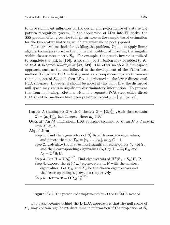
Section 9.4. Face Recognition 425
to have significant influences on the design and performance of a statisticalpattern recognition system. In the application of LDA into FR tasks, theSSS problem often gives rise to high variance in the sample-based estimationfor the two scatter matrices, which are either ill- or poorly-posed.
There are two methods for tackling the problem. One is to apply linearalgebra techniques to solve the numerical problem of inverting the singularwithin-class scatter matrix Sw. For example, the pseudo inverse is utilizedto complete the task in [116]. Also, small perturbation may be added to Swso that it becomes nonsingular [49, 139]. The other method is a subspaceapproach, such as the one followed in the development of the Fisherfacesmethod [12], where PCA is firstly used as a pre-processing step to removethe null space of Sw, and then LDA is performed in the lower dimensionalPCA subspace. However, it should be noted at this point that the discardednull space may contain significant discriminatory information. To preventthis from happening, solutions without a separate PCA step, called directLDA (D-LDA) methods have been presented recently in [19, 137, 79].
Input: A training set Z with C classes: Z = ZiCi=1, each class containsZi = zijCi
j=1 face images, where zij ∈ RJ .
Output: An M -dimensional LDA subspace spanned by Ψ, an M × J matrixwith M J .
Algorithm:Step 1. Find the eigenvectors of ΦT
b Φb with non-zero eigenvalues,and denote them as Em = [e1, . . . , em], m ≤ C − 1.
Step 2. Calculate the first m most significant eigenvectors (U) of Sband their corresponding eigenvalues (Λb) by U = ΦbEm andΛb = UTSbU.
Step 3. Let H = UΛ−1/2b . Find eigenvectors of HT (Sb + Sw)H, P.
Step 4. Choose the M(≤ m) eigenvectors in P with the smallesteigenvalues. Let PM and Λw be the chosen eigenvectors andtheir corresponding eigenvalues respectively.
Step 5. Return Ψ = HPMΛ−1/2w .
Figure 9.23. The pseudo code implementation of the LD-LDA method
The basic premise behind the D-LDA approach is that the null space ofSw may contain significant discriminant information if the projection of Sb

426 Face Detection, Alignment and Recognition Chapter 9
is not zero in that direction, while no significant information, in terms ofthe maximization in Eq.9.48, will be lost if the null space of Sb is discarded.Based on the theory, it can be concluded that the optimal discriminantfeatures exist in the complement space of the null space of Sb, which hasM = C − 1 nonzero eigenvalues denoted as v = [v1, · · · , vM ]. Let U =[u1, · · · ,uM ] be theM eigenvectors of Sb corresponding to theM eigenvaluesv. The complement space is spanned by U, which is furthermore scaled byH = UΛ−1/2
b so as to have HTSbH = I, where Λb = diag(v), and I is the(M ×M) identity matrix. The projection of Sw in the subspace spannedby H, HTSwH, is then estimated using sample analogs. However, whenthe number of training samples per class is very small, even the projectionHTSwH is ill- or poorly-posed. To this end, a modified optimization criterion
represented as Ψ = arg maxΨ
|ΨT SbΨ||ΨT SbΨ+ΨT SwΨ| , was introduced in the D-LDA
of [79] (hereafter LD-LDA) instead of Eq.9.48 used in the D-LDA of [137](hereafter YD-LDA). As will be seen later, the modified criterion introducesa considerable degree of regularization, which helps to reduce the variance ofthe sample-based estimates in ill- or poorly-posed situations. The detailedprocess to implement the LD-LDA method is depicted in Fig. 9.23.
The classification performance of traditional LDA may be degraded bythe fact that their separability criteria are not directly related to their clas-sification accuracy in the output space [74]. To this end, an extension ofLD-LDA, called DF-LDA is also introduced in [79]. In the DF-LDA method,the output LDA subspace is carefully rotated and re-oriented by an iterativeweighting mechanism introduced into the between-class scatter matrix,
Sb,t =C∑i=1
C∑j=1
ij,t(zi − zj)(zi − zj)T (9.51)
In each iteration, object classes that are closer together in the precedingoutput space, and thus can potentially result in mis-classification, are moreheavily weighted (through ij,t) in the current input space. In this way,the overall separability of the output subspace is gradually enhanced, anddifferent classes tend to be equally spaced after a few iterations.
Gabor Feature Representation
The appearance images of a complex visual object are composed of manylocal structures. The Gabor wavelets are particularly aggressive at captur-ing the features of these local structures corresponding to spatial frequency(scale), spatial localization, and orientation selectively [103]. Consequently,
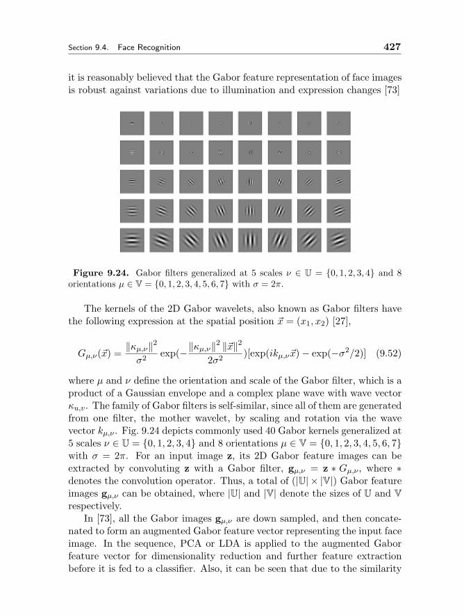
Section 9.4. Face Recognition 427
it is reasonably believed that the Gabor feature representation of face imagesis robust against variations due to illumination and expression changes [73]
Figure 9.24. Gabor filters generalized at 5 scales ν ∈ U = 0, 1, 2, 3, 4 and 8orientations µ ∈ V = 0, 1, 2, 3, 4, 5, 6, 7 with σ = 2π.
The kernels of the 2D Gabor wavelets, also known as Gabor filters havethe following expression at the spatial position x = (x1, x2) [27],
Gµ,ν(x) =‖κµ,ν‖2σ2 exp(−‖κµ,ν‖
2 ‖x‖22σ2 )[exp(ikµ,νx)− exp(−σ2/2)] (9.52)
where µ and ν define the orientation and scale of the Gabor filter, which is aproduct of a Gaussian envelope and a complex plane wave with wave vectorκu,v. The family of Gabor filters is self-similar, since all of them are generatedfrom one filter, the mother wavelet, by scaling and rotation via the wavevector kµ,ν . Fig. 9.24 depicts commonly used 40 Gabor kernels generalized at5 scales ν ∈ U = 0, 1, 2, 3, 4 and 8 orientations µ ∈ V = 0, 1, 2, 3, 4, 5, 6, 7with σ = 2π. For an input image z, its 2D Gabor feature images can beextracted by convoluting z with a Gabor filter, gµ,ν = z ∗ Gµ,ν , where ∗denotes the convolution operator. Thus, a total of (|U| × |V|) Gabor featureimages gµ,ν can be obtained, where |U| and |V| denote the sizes of U and V
respectively.In [73], all the Gabor images gµ,ν are down sampled, and then concate-
nated to form an augmented Gabor feature vector representing the input faceimage. In the sequence, PCA or LDA is applied to the augmented Gaborfeature vector for dimensionality reduction and further feature extractionbefore it is fed to a classifier. Also, it can be seen that due to the similarity
428 Face Detection, Alignment and Recognition Chapter 9
between the Gabor filters, there is a great deal of redundancy in the overcom-plete Gabor feature set. To this end, Wiskott et al. [130] proposed to utilizethe Gabor features corresponding to some specific facial landmarks, calledGabor jets instead of the holistic Gabor images. Based on the jet represen-tation, the Elastic Graph Matching (EGM) was then applied for landmarkmatching and face recognition. The Gabor-based EGM method was one ofthe top performers in the 1996/1997 FERET competition [95].
Mixture of Linear Subspaces
Although successful in many circumstances, linear appearance-based meth-ods including the PCA- and LDA-based ones may fail to deliver good per-formance when face patterns are subject to large variations in viewpoints,illumination or facial expression, which result in a highly non convex andcomplex distribution of face images. The limited success of these methodsshould be attributed to their linear nature. A cost effective approach toaddress the non convex distribution is with a mixture of the linear models.The mixture- or ensemble- based approach embodies the principle of “divideand conquer”, by which a complex FR problem is decomposed into a setof simpler ones, in each of which a locally linear pattern distribution canbe generalized and dealt with by a relatively easy linear solution (see e.g.[93, 114, 38, 15, 75, 39, 77]).
From the designer’s point of view, the central issue to the ensemble-basedapproach is to find an appropriate criterion to decompose the complex facemanifold. Existing partition techniques, whether nonparametric clusteringsuch as K-means [48] or model-based clustering such as EM [84], unanimouslyadopt similarity criterion, based on which similar samples are within thesame cluster and dissimilar samples are in different clusters. For example, inthe view-based representation [93], every face pattern is manually assignedto one of several clusters according to its view angle with each cluster cor-responding to a particular view. In the method considered in [114] and [38],the database partitions are automatically implemented using the K-meansand EM clustering algorithms respectively. However, although such criterionmay be optimal in the sense of approximating real face distribution for taskssuch as face reconstruction, face pose estimation and face detection, theymay not be good for the recognition task considered in the section. It is nothard to see that from a classification point of view, the database partitioncriterion should be aimed to maximize the difference or separability betweenclasses within each “divided” subset or cluster, which as a sub-problem thencan be relatively easy to be “conquered” by a linear FR method.
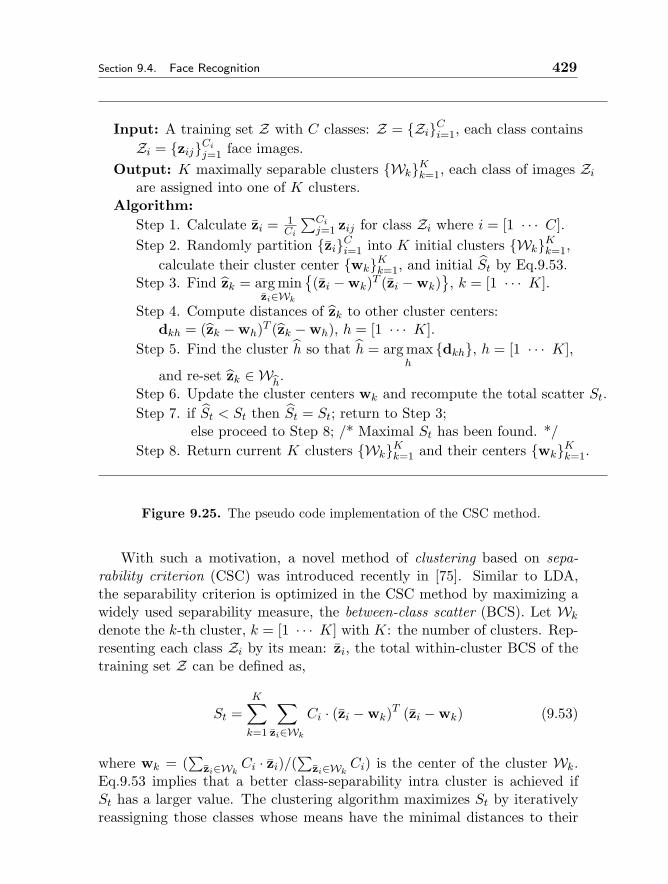
Section 9.4. Face Recognition 429
Input: A training set Z with C classes: Z = ZiCi=1, each class containsZi = zijCi
j=1 face images.Output: K maximally separable clusters WkKk=1, each class of images Zi
are assigned into one of K clusters.Algorithm:
Step 1. Calculate zi = 1Ci
∑Cij=1 zij for class Zi where i = [1 · · · C].
Step 2. Randomly partition ziCi=1 into K initial clusters WkKk=1,calculate their cluster center wkKk=1, and initial St by Eq.9.53.
Step 3. Find zk = arg minzi∈Wk
(zi −wk)T (zi −wk)
, k = [1 · · · K].
Step 4. Compute distances of zk to other cluster centers:dkh = (zk −wh)T (zk −wh), h = [1 · · · K].
Step 5. Find the cluster h so that h = arg maxh
dkh, h = [1 · · · K],
and re-set zk ∈ Wh.
Step 6. Update the cluster centers wk and recompute the total scatter St.Step 7. if St < St then St = St; return to Step 3;
else proceed to Step 8; /* Maximal St has been found. */Step 8. Return current K clusters WkKk=1 and their centers wkKk=1.
Figure 9.25. The pseudo code implementation of the CSC method.
With such a motivation, a novel method of clustering based on sepa-rability criterion (CSC) was introduced recently in [75]. Similar to LDA,the separability criterion is optimized in the CSC method by maximizing awidely used separability measure, the between-class scatter (BCS). Let Wk
denote the k-th cluster, k = [1 · · · K] with K: the number of clusters. Rep-resenting each class Zi by its mean: zi, the total within-cluster BCS of thetraining set Z can be defined as,
St =K∑k=1
∑zi∈Wk
Ci · (zi −wk)T (zi −wk) (9.53)
where wk = (∑
zi∈WkCi · zi)/(
∑zi∈Wk
Ci) is the center of the cluster Wk.Eq.9.53 implies that a better class-separability intra cluster is achieved ifSt has a larger value. The clustering algorithm maximizes St by iterativelyreassigning those classes whose means have the minimal distances to their
430 Face Detection, Alignment and Recognition Chapter 9
own cluster centers, so that the separability between classes is enhancedgradually within each cluster. The maximization process can be implementedby the pseudo codes depicted in Fig. 9.25.
With the CSC process, the training set Z is partitioned into a set of sub-sets WkKk=1 called maximally separable clusters (MSCs). To take advantageof these MSCs, a two-stage hierarchical classification framework (HCF) wasthen proposed in [75]. The HCF consists of a group of FR sub-systems, eachone targeting a specific MSC. This is not a difficult task for most traditionalFR methods such as the YD-LDA [137] used in [75] to work as such a sub-system in a single MSC with limited-size subjects and high between-classseparability.
Nonlinear Subspace Analysis Methods
In addition to the approach using mixture of locally linear models, anotheroption to generate a representation for nonlinear face manifold is with glob-ally nonlinear approach. Recently, the so-called kernel machine techniquehas become one of the most popular tools for designing nonlinear algorithmsin the communities of machine learning and pattern recognition [125, 106].The idea behind the kernel-based learning methods is to construct a non-linear mapping from the input space (RJ) to an implicit high-dimensionalfeature space (F) using a kernel function φ : z ∈ R
J → φ(z) ∈ F. In thefeature space, it is hoped that the distribution of the mapped data is lin-earized and simplified, so that traditional linear methods could perform well.However, the dimensionality of the feature space could be arbitrarily large,possibly infinite. Fortunately, the exact φ(z) is not needed, and the nonlinearmapping can be performed implicitly in R
J by replacing dot products in F
with a kernel function defined in the input space RJ , k(zi, zj) = φ(zi) ·φ(zj).
Examples based on such a design include support vector machines (SVM)[125], kernel PCA (KPCA) [107], kernel ICA (KICA) [6], and GeneralizedDiscriminant Analysis (GDA, also known as kernel LDA) [11].
In the kernel PCA [107], the covariance matrix in F can be expressed as
Scov =1N
C∑i=1
Ci∑j=1
(φ(zij)− φ)(φ(zij)− φ)T (9.54)
where φ = 1N
∑Ci=1∑Ci
j=1 φ(zij) is the average of the ensemble in F. TheKPCA is actually a classic PCA performed in the feature space F. Letgm ∈ F (m = 1, 2, . . . ,M) be the first M most significant eigenvectors ofScov, and they form a low-dimensional subspace, called “KPCA subspace”
Section 9.4. Face Recognition 431
in F. For any face pattern z, its nonlinear principal components can beobtained by the dot product, (gm · (φ(z)− φ)), computed indirectly throughthe kernel function k(). When φ(z) = z, KPCA reduces to PCA, and theKPCA subspace is equivalent to the Eigenface space introduced in [122].
As such, GDA [11] is to extract a nonlinear discriminant feature repre-sentation by performing a classic LDA in the high-dimensional feature spaceF. However, GDA solves the SSS problem in F simply by removing the nullspace of the within-class scatter matrix Sb, although the null space may con-tain the most significant discriminant information as mentioned earlier. Tothis end, a kernel version of LD-LDA [79], also called KDDA, is introducedrecently in [78]. In the feature space, the between- and within-class scattermatrices are given as follows,
Sb =1N
C∑i=1
Ci(φi − φ)(φi − φ)T (9.55)
Sw =1N
C∑i=1
Ci∑j=1
(φ(zij)− φi)(φ(zij)− φi)T (9.56)
where φi = 1Ci
∑Cij=1 φ(zij). Through eigen-analysis of Sb and Sw in the fea-
ture space F, KDDA finds a low-dimensional discriminant subspace spannedby Θ, an M ×N matrix. Any face image z is first nonlinearly transformedto an N × 1 kernel vector,
γ(φ(z)) = [k(z11, z), k(z12, z), · · · , k(zccc , z)]T (9.57)
Then, the KDDA-based feature representation y can be obtained by a linearprojection: y = Θ · γ(φ(z)).
9.4.3 Pattern Classification
Given the feature representation of face objects, a classifier is required tolearn a complex decision function to implement final classification. Whereasthe feature representation optimized for the best discrimination would helpreduce the complexity of the decision function, easy for the classifier design,a good classifier would be able to further learn the separability betweensubjects.
Nearest Feature Line Classifier
The nearest neighbor (NN) is a simplest yet most popular method for tem-plate matching. In the NN based classification, the error rate is determined

432 Face Detection, Alignment and Recognition Chapter 9
by the representational capacity of a prototype face database. The represen-tational capacity depends two issues: (i) how the prototypes are chosen toaccount for possible variations; (ii) how many prototypes are available. How-ever, in practice only a small number of them are available for a face class,typically from one to about a dozen. It is desirable to have a sufficientlylarge number of feature points stored to account for as many variations aspossible. To this end, Stan et al. [64] proposed a method, called the nearestfeature line (NFL), to generalize the representational capacity of availableprototype images.
Figure 9.26. Generalizing two prototype feature points y1 and y2 by the featureline y1y2. A query feature point y is projected onto the line as point b.
The basic assumption behind the NFL method is based on an experi-mental finding, which revealed that although the images of appearances ofthe face patterns may vary significantly due to differences in imaging pa-rameters such as lighting, scale, orientation, etc., these differences have anapproximately linear effect when they are small [121]. Consequently, it isreasonable to use a linear model to interpolate and extrapolate the proto-type feature points belonging to the same class in a feature space specific toface representation such as the Eigenfaces space. In the simplest case, thelinear model is generalized by a feature line (FL), passing through a pair ofprototype points (y1,y2), as depicted in Fig. 9.26. Denoting the FL as y1y2,the FL distance between a query feature point y and y1y2 is defined as
d(y,y1y2) = ‖y − b‖, b = y1 + ς(y2 − y1) (9.58)
where b is y’s projection point on the FL, and ς = (y−y1)·(y2−y1)(y2−y1)·(y2−y1) is a position
parameter relative to y1 and y2. The FL approximates variants of the twoprototypes under variations in illumination and expression, i.e. possible faceimages derived from the two. It virtually provides an infinite number ofprototype feature points of the class. Also, assuming that there are Ci > 1prototype feature points available for class i, a number of Ki = Ci(Ci− 1)/2FLs can be constructed to represent the class, e.g. Ki = 10 when Ci = 5.

Section 9.4. Face Recognition 433
As a result, the representational capacity of the prototype set is significantlyenhanced in this way.
The class label (y) of the query feature point y can be inferred by thefollowing NFL rule,
Decide y = i∗ if d(y,yi∗j∗yi∗k∗) = min1≤i≤C
min1≤j<k≤Ci
d(y,yijyik) (9.59)
The classification results do not only determine the class label y, but alsoprovide a quantitative position number ς∗ as a by-product which can be usedto indicate the relative changes (in illumination and expression) between thequery face and the two associated face images yi∗j∗ and yi∗k∗ .
Regularized Bayesian Classifier
LDA has its root in the optimal Bayesian classifier. Let P (y = i) and p(z|y =i) be the prior probability of class i and the class-conditional probabilitydensity of z given the class label is i, respectively. Based on the Bayesformula, we have the following a posteriori probability P (y = i|z), i.e. theprobability of the class label being i given that z has been measured,
P (y = i|z) =p(z|y = i)P (y = i)∑Ci=1 p(z|y = i)P (y = i)
(9.60)
The Bayes decision rule to classify the unlabeled input z is then given as,
Decide y = j if j = arg maxi∈Y
P (y = i|z) (9.61)
The Eq.9.60 is also known as the maximum a posteriori (MAP) rule, and itachieves minimal misclassification risk among all possible decision rules.
The class-conditional densities p(z|y = i) are seldom known. However,often it is reasonable to assume that p(z|y = i) is subjected to a Gaussiandistribution. Let µi and Σi are the mean and covariance matrix of the classi, we have
p(z|y = i) = (2π)−J/2|Σi|−1/2 exp [−di(z)/2] (9.62)
where di(z) = (z− µi)TΣ−1i (z− µi) is the squared Mahalanobis (quadratic)
distance from z to the mean vector µi. With the Gaussian assumption, theclassification rule of Eq.9.61 turns to
Decide y = j if j = arg mini∈Y
(di(z) + ln |Σi| − 2 lnP (y = i)) (9.63)
The decision rule of Eq.9.63 produces quadratic boundaries to separate dif-ferent classes in the J-dimensional real space. Consequently, this is also
434 Face Detection, Alignment and Recognition Chapter 9
referred to as quadratic discriminant analysis (QDA). Often the two statis-tics (µi,Σi) are estimated by their sample analogs,
µi = zi, Σi =1Ci
Ci∑j=1
(zij − zi)(zij − zi)T (9.64)
LDA can be viewed as a special case of QDA when the covariance structureof all classes are identical, i.e. Σi = Σ. However, the estimation for eitherΣi or Σ is ill-posed in the small sample size (SSS) settings, giving rise tohigh variance. This problem becomes extremely severe due to Ci J inFR tasks, where Σi is singular with rank≤ (Ci − 1). To deal with sucha situation, a regularized QDA, built on the D-LDA idea and Friedman’sregularization technique [40], called RD-QDA is introduced recently in [80].The purpose of the regularization is to reduce the variance related to thesample-based estimation for the class covariance matrices at the expense ofpotentially increased bias.
In the RD-QDA method, the face images (zij) are first projected into thebetween-class scatter matrix Sb’s complement null subspace spanned by H,obtaining a representation yij = HTzij . The regularized sample covariancematrix estimate of class i in the subspace spanned by H, denoted by Σi(λ, γ),can be expressed as,
Σi(λ, γ) = (1− γ)Σi(λ) +γ
Mtr[Σi(λ)]I (9.65)
where
Σi(λ) =1
Ci(λ)[(1− λ)Si + λS] , Ci(λ) = (1− λ)Ci + λN (9.66)
Si =Ci∑j=1
(yij − yi)(yij − yi)T , S =C∑i=1
Si = N ·HTSwH (9.67)
yi = HT zi, and (λ, γ) is a pair of regularization parameters. The classifica-tion rule of Eq.9.63 then turns to
Decide y = j if j = arg mini∈Y
(di(y) + ln |Σi(λ, γ)| − 2 lnπi
)(9.68)
where di(y) = (y − yi)T Σ−1i (λ, γ)(y − yi) and πi = Ci/N is the estimate of
the prior probability of class i. The regularization parameter λ (0 ≤ λ ≤ 1)controls the amount that the Si are shrunk toward S. The other parameter
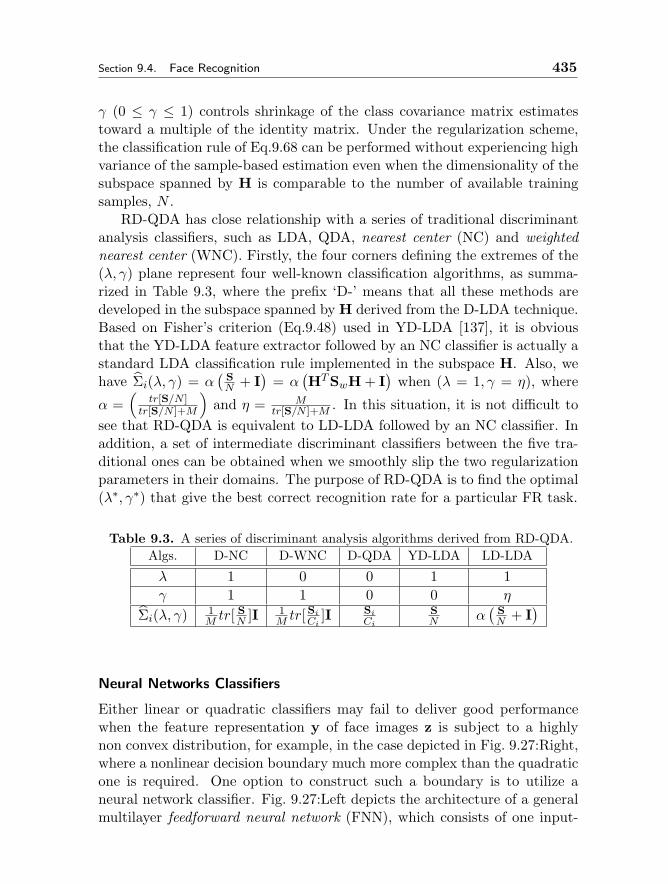
Section 9.4. Face Recognition 435
γ (0 ≤ γ ≤ 1) controls shrinkage of the class covariance matrix estimatestoward a multiple of the identity matrix. Under the regularization scheme,the classification rule of Eq.9.68 can be performed without experiencing highvariance of the sample-based estimation even when the dimensionality of thesubspace spanned by H is comparable to the number of available trainingsamples, N .
RD-QDA has close relationship with a series of traditional discriminantanalysis classifiers, such as LDA, QDA, nearest center (NC) and weightednearest center (WNC). Firstly, the four corners defining the extremes of the(λ, γ) plane represent four well-known classification algorithms, as summa-rized in Table 9.3, where the prefix ‘D-’ means that all these methods aredeveloped in the subspace spanned by H derived from the D-LDA technique.Based on Fisher’s criterion (Eq.9.48) used in YD-LDA [137], it is obviousthat the YD-LDA feature extractor followed by an NC classifier is actually astandard LDA classification rule implemented in the subspace H. Also, wehave Σi(λ, γ) = α
( SN + I
)= α
(HTSwH + I
)when (λ = 1, γ = η), where
α =(
tr[S/N ]tr[S/N ]+M
)and η = M
tr[S/N ]+M . In this situation, it is not difficult tosee that RD-QDA is equivalent to LD-LDA followed by an NC classifier. Inaddition, a set of intermediate discriminant classifiers between the five tra-ditional ones can be obtained when we smoothly slip the two regularizationparameters in their domains. The purpose of RD-QDA is to find the optimal(λ∗, γ∗) that give the best correct recognition rate for a particular FR task.
Table 9.3. A series of discriminant analysis algorithms derived from RD-QDA.Algs. D-NC D-WNC D-QDA YD-LDA LD-LDA
λ 1 0 0 1 1γ 1 1 0 0 η
Σi(λ, γ) 1M tr[
SN ]I 1
M tr[SiCi
]I SiCi
SN α
( SN + I
)
Neural Networks Classifiers
Either linear or quadratic classifiers may fail to deliver good performancewhen the feature representation y of face images z is subject to a highlynon convex distribution, for example, in the case depicted in Fig. 9.27:Right,where a nonlinear decision boundary much more complex than the quadraticone is required. One option to construct such a boundary is to utilize aneural network classifier. Fig. 9.27:Left depicts the architecture of a generalmultilayer feedforward neural network (FNN), which consists of one input-
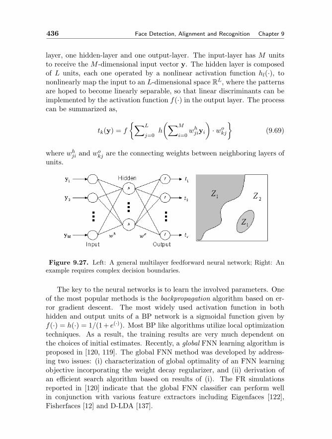
436 Face Detection, Alignment and Recognition Chapter 9
layer, one hidden-layer and one output-layer. The input-layer has M unitsto receive the M -dimensional input vector y. The hidden layer is composedof L units, each one operated by a nonlinear activation function hl(·), tononlinearly map the input to an L-dimensional space R
L, where the patternsare hoped to become linearly separable, so that linear discriminants can beimplemented by the activation function f(·) in the output layer. The processcan be summarized as,
tk(y) = f
∑L
j=0h
(∑M
i=0whjiyi
)· wokj
(9.69)
where whji and wokj are the connecting weights between neighboring layers ofunits.
Figure 9.27. Left: A general multilayer feedforward neural network; Right: Anexample requires complex decision boundaries.
The key to the neural networks is to learn the involved parameters. Oneof the most popular methods is the backpropagation algorithm based on er-ror gradient descent. The most widely used activation function in bothhidden and output units of a BP network is a sigmoidal function given byf(·) = h(·) = 1/(1+ e(·)). Most BP like algorithms utilize local optimizationtechniques. As a result, the training results are very much dependent onthe choices of initial estimates. Recently, a global FNN learning algorithm isproposed in [120, 119]. The global FNN method was developed by address-ing two issues: (i) characterization of global optimality of an FNN learningobjective incorporating the weight decay regularizer, and (ii) derivation ofan efficient search algorithm based on results of (i). The FR simulationsreported in [120] indicate that the global FNN classifier can perform wellin conjunction with various feature extractors including Eigenfaces [122],Fisherfaces [12] and D-LDA [137].
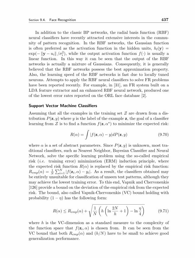
Section 9.4. Face Recognition 437
In addition to the classic BP networks, the radial basis function (RBF)neural classifiers have recently attracted extensive interests in the commu-nity of pattern recognition. In the RBF networks, the Gaussian functionis often preferred as the activation function in the hidden units, hl(y) =exp(−‖y − ui‖ /σ2
i ), while the output activation function f(·) is usually alinear function. In this way it can be seen that the output of the RBFnetworks is actually a mixture of Gaussians. Consequently, it is generallybelieved that the RBF networks possess the best approximation property.Also, the learning speed of the RBF networks is fast due to locally tunedneurons. Attempts to apply the RBF neural classifiers to solve FR problemshave been reported recently. For example, in [31], an FR system built on aLDA feature extractor and an enhanced RBF neural network, produced oneof the lowest error rates reported on the ORL face database [2].
Support Vector Machine Classifiers
Assuming that all the examples in the training set Z are drawn from a dis-tribution P (z, y) where y is the label of the example z, the goal of a classifierlearning from Z is to find a function f(z, α∗) to minimize the expected risk:
R(α) =∫|f(z, α)− y|dP (z, y) (9.70)
where α is a set of abstract parameters. Since P (z, y) is unknown, most tra-ditional classifiers, such as Nearest Neighbor, Bayesian Classifier and NeuralNetwork, solve the specific learning problem using the so-called empiricalrisk (i.e. training error) minimization (ERM) induction principle, wherethe expected risk function R(α) is replaced by the empirical risk function:Remp(α) = 1
N
∑Ni=1 |f(zi, α)− yi|. As a result, the classifiers obtained may
be entirely unsuitable for classification of unseen test patterns, although theymay achieve the lowest training error. To this end, Vapnik and Chervonenkis[126] provide a bound on the deviation of the empirical risk from the expectedrisk. The bound, also called Vapnik-Chervonenkis (VC) bound holding withprobability (1− η) has the following form:
R(α) ≤ Remp(α) +
√1N
(h
(ln
2Nh
+ 1)− ln
η
4
)(9.71)
where h is the VC-dimension as a standard measure to the complexity ofthe function space that f(zi, α) is chosen from. It can be seen from theVC bound that both Remp(α) and (h/N) have to be small to achieve goodgeneralization performance.
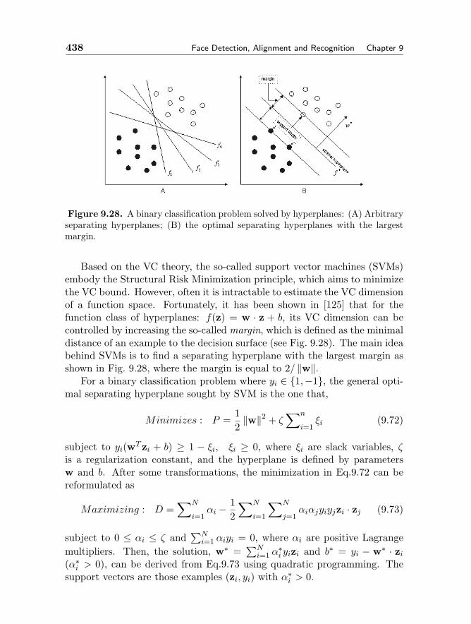
438 Face Detection, Alignment and Recognition Chapter 9
Figure 9.28. A binary classification problem solved by hyperplanes: (A) Arbitraryseparating hyperplanes; (B) the optimal separating hyperplanes with the largestmargin.
Based on the VC theory, the so-called support vector machines (SVMs)embody the Structural Risk Minimization principle, which aims to minimizethe VC bound. However, often it is intractable to estimate the VC dimensionof a function space. Fortunately, it has been shown in [125] that for thefunction class of hyperplanes: f(z) = w · z + b, its VC dimension can becontrolled by increasing the so-called margin, which is defined as the minimaldistance of an example to the decision surface (see Fig. 9.28). The main ideabehind SVMs is to find a separating hyperplane with the largest margin asshown in Fig. 9.28, where the margin is equal to 2/ ‖w‖.
For a binary classification problem where yi ∈ 1,−1, the general opti-mal separating hyperplane sought by SVM is the one that,
Minimizes : P =12‖w‖2 + ζ
∑n
i=1ξi (9.72)
subject to yi(wTzi + b) ≥ 1 − ξi, ξi ≥ 0, where ξi are slack variables, ζis a regularization constant, and the hyperplane is defined by parametersw and b. After some transformations, the minimization in Eq.9.72 can bereformulated as
Maximizing : D =∑N
i=1αi − 1
2
∑N
i=1
∑N
j=1αiαjyiyjzi · zj (9.73)
subject to 0 ≤ αi ≤ ζ and∑N
i=1 αiyi = 0, where αi are positive Lagrangemultipliers. Then, the solution, w∗ =
∑Ni=1 α
∗i yizi and b∗ = yi − w∗ · zi
(α∗i > 0), can be derived from Eq.9.73 using quadratic programming. The
support vectors are those examples (zi, yi) with α∗i > 0.
Section 9.4. Face Recognition 439
For a new data point z, the classification is performed by a decisionfunction,
f(z) = sign (w∗ · z + b∗) = sign
(∑N
i=1α∗i yi(zi · z) + b∗
)(9.74)
In the case where the decision function is not a linear function of thedata, SVMs firstly map the input vector z into a high dimensional featurespace by a nonlinear function φ(z), and then construct an optimal separat-ing hyperplane in the high dimensional space with linear properties. Themapping φ(z) is implemented using kernel machine techniques as it is donein KPCA and GDA. Examples of applying SVMs into the FR tasks can befound in [94, 56, 47, 76].
9.4.4 Evaluation
In this section, we introduce several experiments from our recent studies onsubspace analysis methods. Following standard FR practices, any evaluationdatabase (G) used here is randomly partitioned into two subsets: the trainingset Z and the test set Q. The training set consists of N(=
∑Ci=1Ci) images:
Ci images per subject are randomly chosen. The remaining images are usedto form the test set Q = G − Z. Any FR method evaluated here is firsttrained with Z, and the resulting face recognizer is then applied to Q toobtain a correct recognition rate (CRR), which is defined as the fractionof the test examples correctly classified. To enhance the accuracy of theassessment, all the CRRs reported here are averaged over ≥ 5 runs. Eachrun is executed on a random partition of the database G into Z and Q.
Linear and Quadratic Subspace Analysis
The experiment is designed to assess the performance of various linear andquadratic subspace analysis methods including Eigenfaces, YD-LDA, LD-LDA, RD-QDA and those listed in Table 9.3. The evaluation database usedin the experiment is a middle-size subset of the FERET database. Thesubset consists of 606 gray-scale images of 49 subjects, each one having morethan 10 samples. The performance is evaluated in terms of the CRR andthe sensitivity of the CRR measure to the SSS problem, which depends onthe number of training examples per subject Ci. To this end, six tests wereperformed with various values of Ci ranging from Ci = 2 to Ci = 7.
The CRRs obtained by RD-QDA in the (λ, γ) grid are depicted in Fig. 9.29.Also, a quantitative comparison of the best found CRRs and their corre-sponding parameters among the seven methods is summarized in Table 9.4.

440 Face Detection, Alignment and Recognition Chapter 9
Figure 9.29. CRRs obtained by RD-QDA as functions of (λ, γ). Top: Ci = 2, 3, 4;Bottom: Ci = 5, 6, 7.
The parameter λ controls the degree of shrinkage of the individual class co-variance matrix estimates Si toward the within-class scatter matrix, (HTSwH).Varying the values of λ within [0, 1] leads to a set of intermediate classifiersbetween D-QDA and YD-LDA. In theory, D-QDA should be the best per-former among the methods evaluated here if sufficient training samples areavailable. It can be observed at this point from Fig. 9.29 that the CRRpeaks gradually moved from the central area toward the corner (0, 0) thatis the case of D-QDA as Ci increases. Small values of λ have been goodenough for the regularization requirement in many cases (Ci ≥ 3). How-ever, both of D-QDA and YD-LDA performed poorly when Ci = 2. Thisshould be attributed to the high variance of the estimates of Si and S dueto insufficient training samples. In this case, Si and even S are singularor close to singular, and the resulting effect is to dramatically exaggeratethe importance associated with the eigenvectors corresponding to the small-est eigenvalues. Against the effect, the introduction of another parameterγ helps to decrease the larger eigenvalues and increase the smaller ones,thereby counteracting for some extent the bias. This is also why LD-LDAgreatly outperformed YD-LDA when Ci = 2. Although LD-LDA seems tobe a little over-regularized compared to the optimal RD-QDA(λ∗, γ∗), themethod almost guarantees a stable sub-optimal solution. A CRR differenceof 4.5% on average over the range Ci ∈ [2, 7] has been observed between thetop performer RD-QDA(λ∗, γ∗) and LD-LDA. It can be concluded therefore
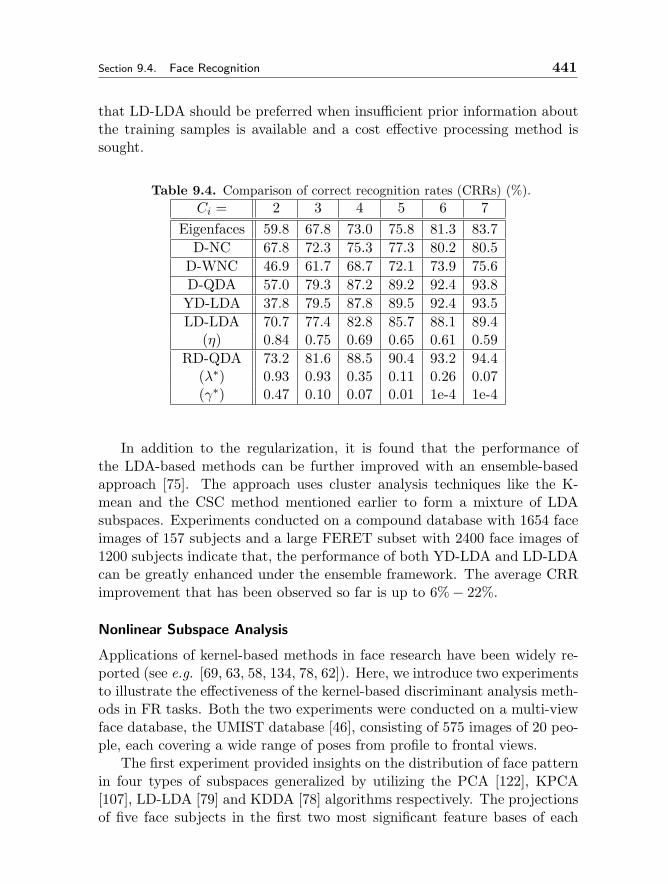
Section 9.4. Face Recognition 441
that LD-LDA should be preferred when insufficient prior information aboutthe training samples is available and a cost effective processing method issought.
Table 9.4. Comparison of correct recognition rates (CRRs) (%).Ci = 2 3 4 5 6 7
Eigenfaces 59.8 67.8 73.0 75.8 81.3 83.7D-NC 67.8 72.3 75.3 77.3 80.2 80.5
D-WNC 46.9 61.7 68.7 72.1 73.9 75.6D-QDA 57.0 79.3 87.2 89.2 92.4 93.8YD-LDA 37.8 79.5 87.8 89.5 92.4 93.5LD-LDA 70.7 77.4 82.8 85.7 88.1 89.4
(η) 0.84 0.75 0.69 0.65 0.61 0.59RD-QDA 73.2 81.6 88.5 90.4 93.2 94.4
(λ∗) 0.93 0.93 0.35 0.11 0.26 0.07(γ∗) 0.47 0.10 0.07 0.01 1e-4 1e-4
In addition to the regularization, it is found that the performance ofthe LDA-based methods can be further improved with an ensemble-basedapproach [75]. The approach uses cluster analysis techniques like the K-mean and the CSC method mentioned earlier to form a mixture of LDAsubspaces. Experiments conducted on a compound database with 1654 faceimages of 157 subjects and a large FERET subset with 2400 face images of1200 subjects indicate that, the performance of both YD-LDA and LD-LDAcan be greatly enhanced under the ensemble framework. The average CRRimprovement that has been observed so far is up to 6%− 22%.
Nonlinear Subspace Analysis
Applications of kernel-based methods in face research have been widely re-ported (see e.g. [69, 63, 58, 134, 78, 62]). Here, we introduce two experimentsto illustrate the effectiveness of the kernel-based discriminant analysis meth-ods in FR tasks. Both the two experiments were conducted on a multi-viewface database, the UMIST database [46], consisting of 575 images of 20 peo-ple, each covering a wide range of poses from profile to frontal views.
The first experiment provided insights on the distribution of face patternin four types of subspaces generalized by utilizing the PCA [122], KPCA[107], LD-LDA [79] and KDDA [78] algorithms respectively. The projectionsof five face subjects in the first two most significant feature bases of each
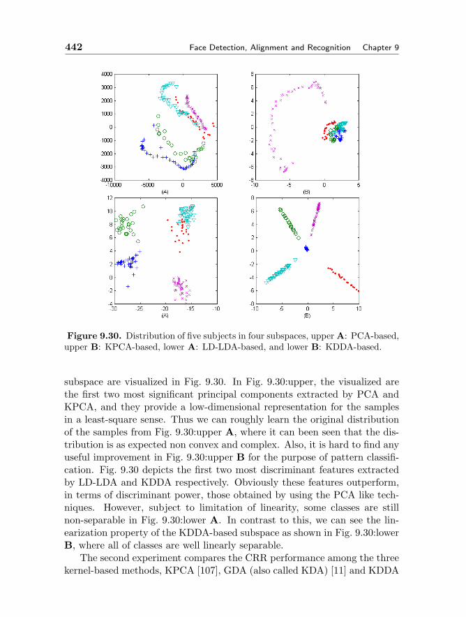
442 Face Detection, Alignment and Recognition Chapter 9
Figure 9.30. Distribution of five subjects in four subspaces, upper A: PCA-based,upper B: KPCA-based, lower A: LD-LDA-based, and lower B: KDDA-based.
subspace are visualized in Fig. 9.30. In Fig. 9.30:upper, the visualized arethe first two most significant principal components extracted by PCA andKPCA, and they provide a low-dimensional representation for the samplesin a least-square sense. Thus we can roughly learn the original distributionof the samples from Fig. 9.30:upper A, where it can been seen that the dis-tribution is as expected non convex and complex. Also, it is hard to find anyuseful improvement in Fig. 9.30:upper B for the purpose of pattern classifi-cation. Fig. 9.30 depicts the first two most discriminant features extractedby LD-LDA and KDDA respectively. Obviously these features outperform,in terms of discriminant power, those obtained by using the PCA like tech-niques. However, subject to limitation of linearity, some classes are stillnon-separable in Fig. 9.30:lower A. In contrast to this, we can see the lin-earization property of the KDDA-based subspace as shown in Fig. 9.30:lowerB, where all of classes are well linearly separable.
The second experiment compares the CRR performance among the threekernel-based methods, KPCA [107], GDA (also called KDA) [11] and KDDA
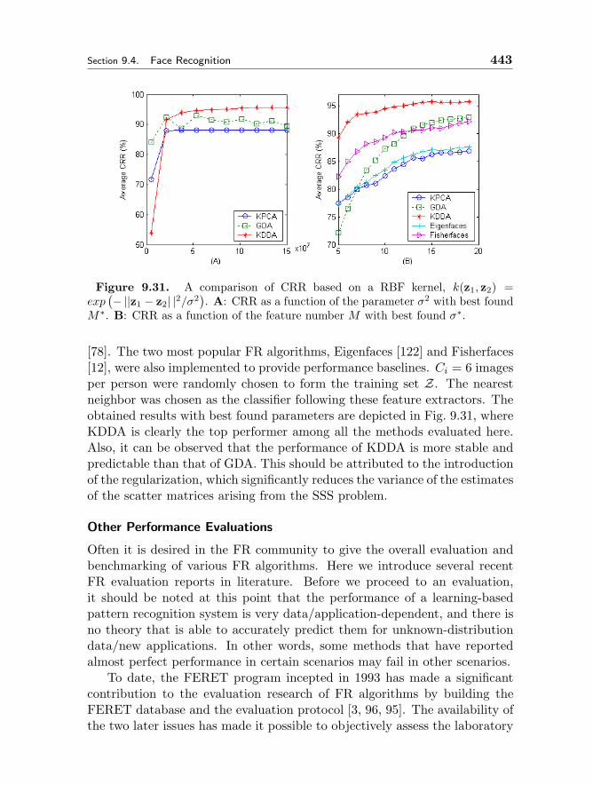
Section 9.4. Face Recognition 443
Figure 9.31. A comparison of CRR based on a RBF kernel, k(z1, z2) =exp
(− ||z1 − z2| |2/σ2). A: CRR as a function of the parameter σ2 with best found
M∗. B: CRR as a function of the feature number M with best found σ∗.
[78]. The two most popular FR algorithms, Eigenfaces [122] and Fisherfaces[12], were also implemented to provide performance baselines. Ci = 6 imagesper person were randomly chosen to form the training set Z. The nearestneighbor was chosen as the classifier following these feature extractors. Theobtained results with best found parameters are depicted in Fig. 9.31, whereKDDA is clearly the top performer among all the methods evaluated here.Also, it can be observed that the performance of KDDA is more stable andpredictable than that of GDA. This should be attributed to the introductionof the regularization, which significantly reduces the variance of the estimatesof the scatter matrices arising from the SSS problem.
Other Performance Evaluations
Often it is desired in the FR community to give the overall evaluation andbenchmarking of various FR algorithms. Here we introduce several recentFR evaluation reports in literature. Before we proceed to an evaluation,it should be noted at this point that the performance of a learning-basedpattern recognition system is very data/application-dependent, and there isno theory that is able to accurately predict them for unknown-distributiondata/new applications. In other words, some methods that have reportedalmost perfect performance in certain scenarios may fail in other scenarios.
To date, the FERET program incepted in 1993 has made a significantcontribution to the evaluation research of FR algorithms by building theFERET database and the evaluation protocol [3, 96, 95]. The availability ofthe two later issues has made it possible to objectively assess the laboratory
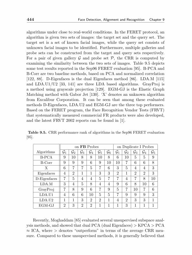
444 Face Detection, Alignment and Recognition Chapter 9
algorithms under close to real-world conditions. In the FERET protocol, analgorithm is given two sets of images: the target set and the query set. Thetarget set is a set of known facial images, while the query set consists ofunknown facial images to be identified. Furthermore, multiple galleries andprobe sets can be constructed from the target and query sets respectively.For a pair of given gallery G and probe set P, the CRR is computed byexamining the similarity between the two sets of images. Table 9.5 depictssome test results reported in the Sep96 FERET evaluation [95]. B-PCA andB-Corr are two baseline methods, based on PCA and normalized correlation[122, 88]. D-Eigenfaces is the dual Eigenfaces method [86]. LDA.M [115]and LDA.U1/U2 [33, 141] are three LDA based algorithms. GrayProj isa method using grayscale projection [129]. EGM-GJ is the Elastic GraphMatching method with Gabor Jet [130]. ‘X’ denotes an unknown algorithmfrom Excalibur Corporation. It can be seen that among these evaluatedmethods D-Eigenfaces, LDA.U2 and EGM-GJ are the three top performers.Based on the FERET program, the Face Recognition Vendor Tests (FRVT)that systematically measured commercial FR products were also developed,and the latest FRVT 2002 reports can be found in [1].
Table 9.5. CRR performance rank of algorithms in the Sep96 FERET evaluation[95].
on FB Probes on Duplicate I ProbesAlgorithms G1 G2 G3 G4 G5 G6 G1 G2 G3 G4 G5
B-PCA 9 10 8 8 10 8 6 10 5 5 9B-Corr 9 9 9 6 9 10 10 7 6 6 8
X 6 7 7 5 7 6 3 5 4 4 3Eigenfaces 4 2 1 1 3 3 2 1 2 2 3
D-Eigenfaces 7 5 4 4 5 7 7 4 7 8 10LDA.M 3 4 5 8 4 4 9 6 8 10 6
GrayProj 7 8 9 6 7 9 5 7 10 7 6LDA.U1 4 6 6 10 5 5 7 9 9 9 3LDA.U2 1 1 3 2 2 1 4 2 3 3 1EGM-GJ 2 3 2 2 1 1 1 3 1 1 1
Recently, Moghaddam [85] evaluated several unsupervised subspace anal-ysis methods, and showed that dual PCA (dual Eigenfaces) > KPCA > PCA≈ ICA, where > denotes “outperform” in terms of the average CRR mea-sure. Compared to these unsupervised methods, it is generally believed that
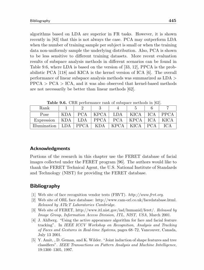
Bibliography 445
algorithms based on LDA are superior in FR tasks. However, it is shownrecently in [83] that this is not always the case. PCA may outperform LDAwhen the number of training sample per subject is small or when the trainingdata non-uniformly sample the underlying distribution. Also, PCA is shownto be less sensitive to different training datasets. More recent evaluationresults of subspace analysis methods in different scenarios can be found inTable 9.6, where LDA is based on the version of [33, 12], PPCA is the prob-abilistic PCA [118] and KICA is the kernel version of ICA [6]. The overallperformance of linear subspace analysis methods was summarized as LDA >PPCA > PCA > ICA, and it was also observed that kernel-based methodsare not necessarily be better than linear methods [62].
Table 9.6. CRR performance rank of subspace methods in [62].Rank 1 2 3 4 5 6 7Pose KDA PCA KPCA LDA KICA ICA PPCA
Expression KDA LDA PPCA PCA KPCA ICA KICAIllumination LDA PPCA KDA KPCA KICA PCA ICA
Acknowledgments
Portions of the research in this chapter use the FERET database of facialimages collected under the FERET program [96]. The authors would like tothank the FERET Technical Agent, the U.S. National Institute of Standardsand Technology (NIST) for providing the FERET database.
Bibliography
[1] Web site of face recognition vendor tests (FRVT). http://www.frvt.org.[2] Web site of ORL face database: http://www.cam-orl.co.uk/facedatabase.html.
Released by AT&T Laboratories Cambridge.[3] Web site of FERET, http://www.itl.nist.gov/iad/humanid/feret/. Released by
Image Group, Information Access Division, ITL, NIST, USA, March 2001.[4] J. Ahlberg. “Using the active appearance algorithm for face and facial feature
tracking”. In IEEE ICCV Workshop on Recognition, Analysis and Trackingof Faces and Gestures in Real-time Systems, pages 68–72, Vancouver, Canada,July 13 2001.
[5] Y. Amit, , D. Geman, and K. Wilder. “Joint induction of shape features and treeclassifiers”. IEEE Transactions on Pattern Analysis and Machine Intelligence,19:1300–1305, 1997.
446 Face Detection, Alignment and Recognition Chapter 9
[6] F. R. Bach and M. I. Jordan. “Kernel independent component analysis”. Com-puter Science Division, University of California Berkeley, Available as Techni-cal Report No. UCB/CSD-01-1166, November 2001.
[7] S. Baker and I. Matthews. “Equivalence and efficiency of image alignment al-gorithms”. In Proceedings of IEEE Computer Society Conference on ComputerVision and Pattern Recognition, volume 1, pages 1090–1097, Hawaii, December11-13 2001.
[8] S. Baker and S. Nayar. “Pattern rejection”. In Proceedings of IEEE ComputerSociety Conference on Computer Vision and Pattern Recognition, pages 544–549, June 1996.
[9] M. Bartlett, J. Movellan, and T. Sejnowski. “Face recognition by independentcomponent analysis”. IEEE Transactions on Neural Networks, 13(6):1450–1464, Nov. 2002.
[10] M. S. Bartlett, H. M. Lades, and T. J. Sejnowski. Independent componentrepresentations for face recognition. Proceedings of the SPIE, Conference onHuman Vision and Electronic Imaging III, 3299:528–539, 1998.
[11] G. Baudat and F. Anouar. “Generalized discriminant analysis using a kernelapproach”. Neural Computation, 12:2385–2404, 2000.
[12] P. N. Belhumeur, J. P. Hespanha, and D. J. Kriegman. “Eigenfaces vs. Fisher-faces: Recognition using class specific linear projection. IEEE Transactions onPattern Analysis and Machine Intelligence, 19(7):711–720, July 1997.
[13] D. Beymer. “Vectorizing face images by interleaving shape and texture com-putations”. A. I. Memo 1537, MIT, 1995.
[14] M. Bichsel and A. P. Pentland. “Human face recognition and the face imageset’s topology”. CVGIP: Image Understanding, 59:254–261, 1994.
[15] C. M. Bishop and J. M. Winn. “Non-linear bayesian image modelling”. InECCV (1), pages 3–17, 2000.
[16] V. Blanz and T.Vetter. “A morphable model for the synthesis of 3d faces”. InSIGGRAPH’99 Conference Proceedings, pages 187–194, 1999.
[17] R. Brunelli and T. Poggio. “Face recognition: Features versus templates”. IEEETransactions on Pattern Analysis and Machine Intelligence, 15(10):1042–1052,1993.
[18] R. Chellappa, C. Wilson, and S. Sirohey. “Human and machine recognition offaces: A survey”. PIEEE, 83:705–740, 1995.
[19] L.-F. Chen, H.-Y. M. Liao, M.-T. Ko, J.-C. Lin, and G.-J. Yu. “A new LDA-based face recognition system which can solve the small sample size problem”.Pattern Recognition, 33:1713–1726, 2000.
[20] L.-F. Chen, H.-Y. M. Liao, J.-C. Lin, and C.-C. Han. “Why recognition ina statistics-based face recognition system should be based on the pure faceportion: a probabilistic decision-based proof”. Pattern Recognition, 34(7):1393–1403, 2001.
[21] T. Cootes and C. Taylor. ”Constrained active appearance models”. Proceedingsof IEEE International Conference on Computer Vision, 1:748–754, 2001.
[22] T. F. Cootes, G. J. Edwards, and C. J. Taylor. Active appearance models. InECCV98, volume 2, pages 484–498, 1998.
Bibliography 447
[23] T. F. Cootes, C. J. Taylor, D. H. Cooper, and J. Graham. “Active shape models:Their training and application”. CVGIP: Image Understanding, 61:38–59, 1995.
[24] T. F. Cootes, K. N. Walker, and C. J. Taylor. View-based active appearancemodels. In Proc. Int. Conf. on Face and Gesture Recognition, pages 227–232,2000.
[25] I. J. Cox, J. Ghosn, and P. Yianilos. “Feature-based face recognition usingmixture-distance”. In Proceedings of IEEE Computer Society Conference onComputer Vision and Pattern Recognition, pages 209–216, 1996.
[26] F. Crow. “Summed-area tables for texture mapping”. In SIGGRAPH, volume18(3), pages 207–212, 1984.
[27] J. G. Daugman. “Complete discrete 2-d gabor transform by neural networkfor image analysis and compression”. IEEE Trans. On Acoustics, Speech andSignal Processing, 36(7):1169–1179, July 1988.
[28] N. Duta, A. Jain, and M. Dubuisson-Jolly. ”automatic construction of 2-d shapemodels”. IEEE Transactions on Pattern Analysis and Machine Intelligence,23(5):433–446, 2001.
[29] G. J. Edwards, T. F. Cootes, and C. J. Taylor. “Face recognition using activeappearance models”. In Proceedings of the European Conference on ComputerVision, volume 2, pages 581–695, 1998.
[30] M. Elad, Y. Hel-Or, and R. Keshet. “Pattern detection using a maximal rejec-tion classifier”. Pattern Recognition Letters, 23:1459–1471, October 2002.
[31] M. J. Er, S. Wu, J. Lu, and H. L. Toh. “Face recognition with radial basisfunction (RBF) neural networks”. IEEE Transactions on Neural Networks,13(3):697–710, May 2002.
[32] B. K. L. Erik Hjelmas. “Face detection: A survey”. Computer Vision andImage Understanding, 3(3):236–274, September 2001.
[33] K. Etemad and R. Chellappa. “Discriminant analysis for recognition of humanface images”. J. Optical Soc. Am. A, 14(8):1724–1733, August 1997.
[34] J. Feraud, O. Bernier, and M. Collobert. “A fast and accurate face detectorfor indexation of face images”. In Proc. Fourth IEEE Int. Conf on AutomaticFace and Gesture Recognition, Grenoble, 2000.
[35] R. Fisher. “The use of multiple measures in taxonomic problems”. Ann. Eu-genics, 7:179–188, 1936.
[36] F. Fleuret and D. Geman. “Coarse-to-fine face detection”. International Jour-nal of Computer Vision, 20:1157–1163, 2001.
[37] Y. Freund and R. Schapire. “A decision-theoretic generalization of on-linelearning and an application to boosting”. Journal of Computer and SystemSciences, 55(1):119–139, August 1997.
[38] B. J. Frey, A. Colmenarez, and T. S. Huang. “Mixtures of local linear subspacesfor face recognition”. In Proceedings of The IEEE Conference on ComputerVision and Pattern Recognition, Santa Barbara, CA, June 1998.
[39] B. J. Frey and N. Jojic. “Transformation-invariant clustering using the emalgorithm”. IEEE Transactions on Pattern Analysis and Machine Intelligence,25(1):1–17, JANUARY 2003.
[40] J. H. Friedman. “Regularized discriminant analysis”. Journal of the AmericanStatistical Association, 84:165–175, 1989.
448 Face Detection, Alignment and Recognition Chapter 9
[41] R. Frischholz. The face detection homepage. http://home.t-online.de/home/Robert.Frischholz/face.htm.
[42] K. Fukunaga. Introduction to statistical pattern recognition. Academic Press,Boston, 2 edition, 1990.
[43] M. Girolami. “Advances in Independent Component Analysis.”. Springer-Verlag, Berlin, 2000.
[44] A. J. Goldstein, L. D. Harmon, and A. B. Lesk. “Identification of human faces”.Proceedings of the IEEE, 59(5):748–760, May 1971.
[45] S. Gong, S. McKenna, and J. Collins. “An investigation into face pose distri-bution”. In Proc. IEEE International Conference on Face and Gesture Recog-nition, Vermont, 1996.
[46] D. B. Graham and N. M. Allinson. “Characterizing virtual eigensignatures forgeneral purpose face recognition”. In H. Wechsler, P. J. Phillips, V. Bruce,F. Fogelman-Soulie, and T. S. Huang, editors, Face Recognition: From Theoryto Applications, NATO ASI Series F, Computer and Systems Sciences, volume163, pages 446–456. 1998.
[47] G. Guo, S. Li, and K. Chan. “Face recognition by support vector machines”. InProceedings of Fourth IEEE International Conference on Automatic Face andGesture Recognition 2000, Grenoble, France, March 2000.
[48] J. Hartigan. “Statistical theory in clustering”. Journal of Classification, 2:63–76, 1985.
[49] Z.-Q. Hong and J.-Y. Yang. “Optimal discriminant plane for a small numberof samples and design method of classifier on the plane”. Pattern Recognition,24(4):317–324, 1991.
[50] X. W. Hou, S. Z. Li, and H. J. Zhang. “Direct appearance models”. In Proceed-ings of IEEE Computer Society Conference on Computer Vision and PatternRecognition, volume 1, pages 828–833, Hawaii, December 11-13 2001.
[51] J. Huang, X. Shao, and H. Wechsler. “Face pose discrimination using supportvector machines (SVM)”. In Proceedings of International Conference PatternRecognition, Brisbane, Queensland, Australia, 1998.
[52] A. Hyvrinen and P. Hoyer. “Emergence of phase and shift invariant features bydecomposition of natural images into independent feature subspaces”. NeuralComputation, 12:1705–1720, 2000.
[53] A. Hyvrinen and P. Hoyer. “Emergence of topography and complex cell prop-erties from natural images using extensions of ica”. In Proceedings of Advancesin Neural Information Processing Systems, volume 12, pages 827–833, 2000.
[54] A. Jain and D. Zongker. Feature selection: evaluation, application, and samllsample performance. IEEE Trans. on PAMI, 19(2):153–158, 1997.
[55] L. Jolliffe. Principle Component Analysis. New York: Springer-Verlag, 1986.[56] K. Jonsson, J. Matas, J. Kittler, and Y. Li. “Learning support vectors for
face verification and recognition”. In Proceedings of Fourth IEEE Interna-tional Conference on Automatic Face and Gesture Recognition 2000, Grenoble,France, March 2000.
[57] T. Kanade. Picture Processing by Computer Complex and Recognition of Hu-man Faces. PhD thesis, Kyoto University, 1973.

Bibliography 449
[58] K. I. Kim, K. Jung, and H. J. Kim. “Face recognition using kernel principalcomponent analysis”. IEEE Signal Processing Letters, 9(2):40–42, FebFebruary2002.
[59] J. Kittler. “Feature set search algorithm”. In C. H. Chen, editor, PatternRecognition in Practice, pages 41–60. NorthHolland, Sijthoff and Noordhoof,1980.
[60] A. Kuchinsky, C. Pering, M. L. Creech, D. Freeze, B. Serra, and J. Gwizdka.”FotoFile: A consumer multimedia organization and retrieval system”. In Pro-ceedings of ACM SIG CHI’99 Conference, Pittsburg, May 1999.
[61] T.-W. Lee. “Independent Component Analysis: Theory and Applications.”.Kluwer Academic, 1998.
[62] J. Li, S. Zhou, and C. Shekhar. “A comparison of subspace analysis for facerecognition”. In Proceedings of the 28th IEEE International Conference onAcoustics, Speech, and Signal Processing, Hong Kong, China, April 2003.
[63] S. Z. Li, Q. D. Fu, L. Gu, B. Scholkopf, Y. M. Cheng, and H. J. Zhang. “Kernelmachine based learning for multi-view face detection and pose estimation”. InProceedings of 8th IEEE International Conference on Computer Vision, Van-couver, Canada, July 2001.
[64] S. Z. Li and J. Lu. “Face recognition using the nearest feature line method”.IEEE Transactions on Neural Networks, 10:439–443, March 1999.
[65] S. Z. Li, X. G. Lv, and H. .Zhang. “View-based clustering of object appear-ances based on independent subspace analysis”. In Proceedings of The EighthIEEE International Conference on Computer Vision, volume 2, pages 295–300,Vancouver, Canada, July 2001.
[66] S. Z. Li, S. C. Yan, H. J. Zhang, and Q. S. Cheng. “Multi-view face alignmentusing direct appearance models”. In Proceedings of IEEE International Con-ference on Automatic Face and Gesture Recognition, Washington, DC, 20-21May 2002.
[67] S. Z. Li, Z. Zhang, H.-Y. Shum, and H. Zhang. “FloatBoost learning for clas-sification”. In Proceedings of Neural Information Processing Systems, pages –,Vancouver, Canada, December 9-14 2002.
[68] S. Z. Li, L. Zhu, Z. Q. Zhang, A. Blake, H. Zhang, and H. Shum. “Statisticallearning of multi-view face detection”. In Proceedings of the European Confer-ence on Computer Vision, volume 4, pages 67–81, Copenhagen, Denmark, May28 - June 2 2002.
[69] Y. Li, S. Gong, and H. Liddell. “Constructing facial identity surfaces in anonlinear discriminating space.”. In Proceedings of IEEE Computer SocietyConference on Computer Vision and Pattern Recognition, Hawaii, December2001.
[70] Y. M. Li, S. G. Gong, and H. Liddell. “Support vector regression and classi-fication based multi-view face detection and recognition”. In IEEE Int. Conf.Oo Face & Gesture Recognition, pages 300–305, France, March 2000.
[71] R. Lienhart, A. Kuranov, and V. Pisarevsky. “Empirical analysis of detectioncascades of boosted classifiers for rapid object detection”. Mrl technical report,Intel Labs, Dec 2002.
450 Face Detection, Alignment and Recognition Chapter 9
[72] C. Liu and H. Wechsler. “Comparative assessment of independent componentanalysis (ica) for face recognition”. In Proceedings of the 2nd InternationalConference on Audioand Video-based Biometric Person Authentication, Wash-ington D. C., March 22-24 1999.
[73] C. Liu and H. Wechsler. “Gabor feature based classification using the enhancedfisher linear discriminant model for face recognition”. IEEE Transactions onImage Processing, 11(4):467–476, April 2002.
[74] R. Lotlikar and R. Kothari. “Fractional-step dimensionality reduction”. IEEETransactions on Pattern Analysis and Machine Intelligence, 22(6):623–627,2000.
[75] J. Lu and K. Plataniotis. “Boosting face recognition on a large-scale database”.In Proceedings of the IEEE International Conference on Image Processing,pages II.109–II.112, Rochester, New York, USA, September 2002.
[76] J. Lu, K. Plataniotis, and A. Venetsanopoulos. “Face recognition using featureoptimization and ν-support vector learning”. In Proceedings of the IEEE Inter-national Workshop on Neural Networks for Signal Processing, pages 373–382,Falmouth, MA., USA, September 2001.
[77] J. Lu, K. Plataniotis, and A. Venetsanopoulos. “Boosting linear discriminantanalysis for face recognition”. In Proceedings of the IEEE International Con-ference on Image Processing, Barcelona, Spain, September 2003.
[78] J. Lu, K. Plataniotis, and A. Venetsanopoulos. “Face recognition using kerneldirect discriminant analysis algorithms”. IEEE Transactions on Neural Net-works, 14(1), January 2003.
[79] J. Lu, K. Plataniotis, and A. Venetsanopoulos. “Face recognition using LDAbased algorithms”. IEEE Transactions on Neural Networks, 14(1), January2003.
[80] J. Lu, K. Plataniotis, and A. Venetsanopoulos. “Regularized discriminant anal-ysis for the small sample size problem in face recognition”. Accepted for publi-cation in Pattern Recognition Letter, July 2003.
[81] D. Marr. Vision. W. H. Freeman and Co, San Francisco, 1982.[82] A. Martinez and R. Benavente. “The AR face database”. Technical Report 24,
CVC, June 1998.[83] A. M. Martnez and A. C. Kak. “PCA versus LDA”. IEEE Transactions on
Pattern Analysis and Machine Intelligence, 23(2):228–233, 2001.[84] G. McLachlan and D. Peel. “Finite Mixture Models”. John Wiley & Sons, 2000.[85] B. Moghaddam. “Principal manifolds and probabilistic subspaces for visual
recognition”. IEEE Transactions on Pattern Analysis and Machine Intelligence,24(6):780–788, June 2002.
[86] B. Moghaddam, T. Jebara, and A. Pentland. “Bayesian face recognition”.Pattern Recognition, 33:1771–1782, 2000.
[87] B. Moghaddam and A. Pentland. “Probabilistic visual learning for object repre-sentation”. IEEE Transactions on Pattern Analysis and Machine Intelligence,7:696–710, July 1997.
[88] H. Moon and P. Phillips. “Analysis of pca-based face recognition algorithms”.In K. Bowyer and P. Phillips, editors, Empirical Evaluation Techniques in Com-puter Vision, pages 57–71. Calif.:IEEE CS Press, Los Alamitos, 1998.
Bibliography 451
[89] Y. Moses, Y. Adini, and S. Ullman. “Face recognition: The problem of com-pensating for changes in illumination direction”. In Proceedings of the EuropeanConference on Computer Vision, volume A, pages 286–296, 1994.
[90] J. Ng and S. Gong. “performing multi-view face detection and pose estimationusing a composite support vector machine across the view sphere”. In Proc.IEEE International Workshop on Recognition, Analysis, and Tracking of Facesand Gestures in Real-Time Systems, pages 14–21, Corfu, Greece, September1999.
[91] E. Osuna, R. Freund, and F. Girosi. “Training support vector machines: Anapplication to face detection”. In CVPR, pages 130–136, 1997.
[92] C. P. Papageorgiou, M. Oren, and T. Poggio. “A general framework for objectdetection”. In Proceedings of IEEE International Conference on ComputerVision, pages 555–562, Bombay, India, 1998.
[93] A. P. Pentland, B. Moghaddam, and T. Starner. “View-based and modulareigenspaces for face recognition”. In Proceedings of IEEE Computer SocietyConference on Computer Vision and Pattern Recognition, pages 84–91, 1994.
[94] P. Phillips. “Support vector machines applied to face recognition”. InM. Kearns, S. Solla, and D. Cohn, editors, NIPS’98. 1998.
[95] P. J. Phillips, H. Moon, S. A. Rizvi, and P. J. Rauss. The FERET evaluationmethodology for face-recognition algorithms. IEEE Transactions on PatternAnalysis and Machine Intelligence, 22(10):1090–1104, 2000.
[96] P. J. Phillips, H. Wechsler, J. Huang, and P. Rauss. “The FERET databaseand evaluation procedure for face recognition algorithms”. Image and VisionComputing J, 16(5):295–306, 1998.
[97] P. Pudil, J. Novovicova, and J. Kittler. “Floating search methods in featureselection”. Pattern Recognition Letters, 15(11):1119–1125, 1994.
[98] S. Romdhani, A. Psarrou, and S. Gong. “Learning a single active face shapemodel across views”. In Proc. IEEE International Workshop on Recognition,Analysis, and Tracking of Faces and Gestures in Real-Time Systems, Corfu,Greece, 26-27 September 1999.
[99] D. Roth, M. Yang, and N. Ahuja. “A snow-based face detector”. In Proceedingsof Neural Information Processing Systems, 2000.
[100] H. A. Rowley, S. Baluja, and T. Kanade. “Neural network-based face de-tection”. IEEE Transactions on Pattern Analysis and Machine Intelligence,20(1):23–28, 1998.
[101] A. Samal and P. A.Iyengar. “Automatic recognition and analysis of humanfaces and facial expressions: A survey”. Pattern Recognition, 25:65–77, 1992.
[102] R. Schapire, Y. Freund, P. Bartlett, and W. S. Lee. “Boosting the margin:A new explanation for the effectiveness of voting methods”. The Annals ofStatistics, 26(5):1651–1686, October 1998.
[103] B. Schiele and J. L. Crowley. “Recognition without correspondence using mul-tidimensional receptive field histograms”. International Journal of ComputerVision, 36(1):31–52, 2000.
[104] H. Schneiderman. “A Statistical Approach to 3D Object Detection Applied toFaces and Cars” (CMU-RI-TR-00-06). PhD thesis, RI, 2000.

452 Face Detection, Alignment and Recognition Chapter 9
[105] H. Schneiderman and T. Kanade. “A statistical method for 3d object detectionapplied to faces and cars”. In Proceedings of IEEE Computer Society Conferenceon Computer Vision and Pattern Recognition, 2000.
[106] B. Scholkopf, C. Burges, and A. J. Smola. “Advances in Kernel Methods -Support Vector Learning”. MIT Press, Cambridge, MA, 1999.
[107] B. Scholkopf, A. Smola, and K. R. Muller. Nonlinear component analysis as akernel eigenvalue problem. Neural Computation, 10:1299–1319, 1999.
[108] S. Sclaroff and J. Isidoro. “Active blobs”. In Proceedings of IEEE InternationalConference on Computer Vision, Bombay, India, 1998.
[109] P. Y. Simard, L. Bottou, P. Haffner, and Y. L. Cun. “Boxlets: a fast convolutionalgorithm for signal processing and neural networks”. In M. Kearns, S. Solla,and D. Cohn, editors, Advances in Neural Information Processing Systems,volume 11, pages 571–577. MIT Press, 1998.
[110] P. Y. Simard, Y. A. L. Cun, J. S. Denker, and B. Victorri. “Transformationinvariance in pattern recognition - tangent distance and tangent propagation”.In G. B. Orr and K.-R. Muller, editors, Neural Networks: Tricks of the Trade.Springer, 1998.
[111] L. Sirovich and M. Kirby. “Low-dimensional procedure for the characterizationof human faces”. Journal of the Optical Society of America A, 4(3):519–524,March 1987.
[112] P. Somol, P. Pudil, J. Novoviova, and P. Paclik. “Adaptive floating searchmethods in feature selection”. Pattern Recognition Letters, 20:1157–1163, 1999.
[113] S. D. Stearns. “On selecting features for pattern classifiers”. In Proceedings ofInternational Conference Pattern Recognition, pages 71–75, 1976.
[114] K.-K. Sung and T. Poggio. “Example-based learning for view-based human facedetection”. IEEE Transactions on Pattern Analysis and Machine Intelligence,20(1):39–51, 1998.
[115] D. L. Swets and J. Weng. “Using discriminant eigenfeatures for image re-trieval”. IEEE Transactions on Pattern Analysis and Machine Intelligence,18:831–836, 1996.
[116] Q. Tian, M. Barbero, Z. Gu, and S. Lee. “Image classification by the foley-sammon transform”. Opt. Eng., 25(7):834–840, 1986.
[117] K. Tieu and P. Viola. “Boosting image retrieval”. In Proceedings of IEEEComputer Society Conference on Computer Vision and Pattern Recognition,volume 1, pages 228–235, 2000.
[118] M. Tipping and C. Bishop. “Probabilistic principal component analysis”. Jour-nal of the Royal Statistical Society, Series B., 61:611–622, 1999.
[119] K. A. Toh. “Global optimization by monotonic transformation”. ComputationalOptimization and Applications, 23:77–99, October 2002.
[120] K.-A. Toh, J. Lu, and W.-Y. Yau. “Global feedforward neural network learningfor classification and regression”. In M. Figueiredo, J. Zerubia, and A. K. Jain,editors, Proceedings of the Energy Minimization Methods in Computer Visionand Pattern Recognition, Sophia Antipolis, France, September 3-5 2001.
[121] M. Turk. “A random walk through eigenspace”. IEICE Trans. Inf. & Syst.,E84-D(12):1586–1695, December 2001.
Bibliography 453
[122] M. A. Turk and A. P. Pentland. “Eigenfaces for recognition”. Journal ofCognitive Neuroscience, 3(1):71–86, March 1991.
[123] D. Valentin, H. Abdi, A. J. O’Toole, and G. W. Cottrell. “Connectionist modelsof face processing: A survey”. Pattern Recognition, 27(9):1209–1230, 1994.
[124] B. van Ginneken, A. F. Frangi, J. J. Staal, B. M. ter Haar Romeny, and M. A.Viergever. ”a non-linear gray-level appearance model improves active shapemodel segmentation”. In Proceedings of Mathematical Methods in BiomedicalImage Analysis, 2001.
[125] V. N. Vapnik. “The Nature of Statistical Learning Theory”. Springer-Verlag,New York, 1995.
[126] V. N. Vapnik. “An overview of statistical learning theory”. IEEE Transactionson Neural Networks, 10(5):439–443, September 1999.
[127] P. Viola and M. Jones. “Rapid object detection using a boosted cascade of sim-ple features”. In Proceedings of IEEE Computer Society Conference on Com-puter Vision and Pattern Recognition, Kauai, Hawaii, December 12-14 2001.
[128] P. Viola and M. Jones. “Robust real time object detection”. In IEEE ICCVWorkshop on Statistical and Computational Theories of Vision, Vancouver,Canada, July 13 2001.
[129] J. Wilder. “Face recognition using transform coding of grayscale projectionprojections and the neural tree network”. In R. J. Mammone, editor, Artifi-cial Neural Networks with Appli-cations in Speech and Vision, pages 520–536.Chapman Hall, 1994.
[130] L. Wiskott, J. Fellous, N. Kruger, and C. V. malsburg. ”face recognition byelastic bunch graph matching”. IEEE Transactions on Pattern Analysis andMachine Intelligence, 19(7):775–779, 1997.
[131] S. C. Yan, C. Liu, S. Z. Li, L. Zhu, H. J. Zhang, H. Shum, and Q. Cheng.“Texture-constrained active shape models”. In Proceedings of the First Inter-national Workshop on Generative-Model-Based Vision (with ECCV), Copen-hagen, Denmark, May 2002.
[132] J. Yang, W. Lu, and A. Waibel. “Skin-color modeling and adaptation”. InProceedings of the First Asian Conference on Computer Vision, pages 687–694,1998.
[133] M.-H. Yang. Resources for face detection.http://vision.ai.uiuc.edu/mhyang/face-detection-survey.html.
[134] M.-H. Yang. “Kernel eigenfaces vs. kernel fisherfaces: Face recognition usingkernel methods”. In Proceedings of the Fifth IEEE International Conference onAutomatic Face and Gesture Recognition, Washinton D.C., USA, May 2002.
[135] M.-H. Yang and N. Ahuja. “Gaussian mixture model for human skin colorand its application in image and video databases”. In Proc. of the SPIE Conf.on Storage and Retrieval for Image and Video Databases, volume 3656, pages458–466, San Jose, Jan. 1999.
[136] M.-H. Yang, D. Kriegman, and N. Ahuja. “Detecting faces in images: a survey”.IEEE Transactions on Pattern Analysis and Machine Intelligence, 24(1):34–58,2002.
[137] H. Yu and J. Yang. “A direct lda algorithm for high-dimensional data withapplication to face recognition”. Pattern Recognition, 34:2067–2070, 2001.

454 Face Detection, Alignment and Recognition Chapter 9
[138] B. D. Zarit, B. J. Super, and F. K. H. Quek. “Comparison of five color modelsin skin pixel classification”. In IEEE ICCV Workshop on Recognition, Analysisand Tracking of Faces and Gestures in Real-time Systems, pages 58–63, Corfu,Greece, September 1999.
[139] W. Zhao, R. Chellappa, and J. Phillips. “Subspace linear discriminant analysisfor face recognition”. Technical Report, CS-TR4009, Univ. of Maryland, 1999.
[140] W. Zhao, R. Chellappa, A. Rosenfeld, and P. Phillips. Face recognition: Aliterature survey. Technical Report, CFAR-TR00-948, University of Maryland,2000.
[141] W. Zhao, A. Krishnaswamy, R. Chellappa, D. Swets, and J. Weng. “Discrim-inant analysis of principal components for face recognition”. In H. Wechsler,P. Phillips, V. Bruce, F. Soulie, and T. Huang, editors, Face Recognition: FromTheory to Applications, pages 73–85. Springer-Verlag, 1998.
Chapter 10
PERCEPTUAL INTERFACES
Matthew Turk
and Mathias Kolsch
A keyboard! How quaint.
— Scotty, in the film Star Trek IV: The Voyage Home (1986)
10.1 Introduction
Computer vision research has traditionally been motivated by a few mainareas of application. The most prominent of these include biological visionmodeling, robot navigation and manipulation, surveillance, medical imaging,and various inspection, detection, and recognition tasks. In recent years, anew area, often referred to as perceptual interfaces, has emerged to mo-tivate an increasingly large amount of research within the machine visioncommunity. The general focus of this effort is to integrate multiple per-ceptual modalities (such as computer vision, speech and sound processing,and haptic I/O) into the user interface. For computer vision technology inparticular, the primary aim is to use vision as an effective input modalityin human-computer interaction. Broadly defined, perceptual interfaces arehighly interactive, multimodal interfaces that enable rich, natural, and ef-ficient interaction with computers. More specifically, perceptual interfacesseek to leverage sensing (input) and rendering (output) technologies in orderto provide interactions not feasible with standard interfaces and the commontriumvirate of I/O devices: the keyboard, mouse and monitor.
The motivation behind perceptual interfaces is twofold: (1) the chang-ing nature of computers and (2) the desire for a more powerful, compelling
455
456 Perceptual Interfaces Chapter 10
user experience than what has been available with graphical user inter-faces (GUI) and the associated WIMP (windows, icons, menus, pointing de-vices) implementations. As computers evolve away from their recent past—desktop machines used primarily for word processing, spreadsheet manipula-tion, and information browsing—and move toward new environments with aplethora of computing form factors, uses, and interaction scenarios, the desk-top metaphor will become less relevant and more cumbersome. Keyboard-based alphanumeric input and mouse-based 2D pointing and selection canbe very limiting, and in some cases awkward and inefficient, modes of in-teraction. Neither mouse nor keyboard, for example, is very appropriate forcommunicating 3D information or the subtleties of human emotions.
Moore’s Law has driven computer hardware over the decades, increasingperformance (measured in various ways) exponentially. This observationpredicts an improvement in chip density in five years by a factor of ten; inten years by a factor of one hundred; and in twenty years by a factor of tenthousand. Unfortunately, human capacity does not grow at such a rate (ifat all) so there is a serious problem in scaling human-computer interactionas machines evolve. It is unlikely that a user interface paradigm developedat an early point in the Moore’s Law curve will continue to be appropriatemuch later on.
New computing scenarios, such as in automobiles and other mobile envi-ronments, rule out many traditional approaches to user interaction. Comput-ing is becoming something that permeates daily life, rather than somethingpeople do only at distinct times and places. In order to accommodate awider range of scenarios, tasks, users, and preferences, interfaces must be-come more natural, intuitive, adaptive, and unobtrusive. These are primarygoals of research in perceptual interfaces.
We will certainly need new and different interaction techniques in a worldof small, powerful, connected, ubiquitous computing. Since small, powerful,connected sensing and display technologies should be available, there hasbeen increased interest in building interfaces that use these technologies toleverage the natural human capabilities to communicate via speech, ges-ture, expression, touch, etc. While these are unlikely to completely replacetradition desktop and GUI-based interfaces, they will complement existinginteraction styles and enable new functionality not otherwise possible or con-venient.
In this chapter, we seek to communicate the motivations and goals ofperceptual interfaces, to enumerate the relevant technologies, to discuss theintegration of multiple modalities, and to describe in more detail the role ofcomputer vision in human-computer interaction. We cover vision problems,
Section 10.2. Perceptual Interfaces and HCI 457
constraints, and approaches that are apropos to the area, survey the state ofthe art in computer vision research applied to perceptual interfaces, describeseveral near-term applications, and suggest promising research directions.
10.2 Perceptual Interfaces and HCI
Human-computer interaction (HCI) is the study of people, computer tech-nology, and the ways these influence each other. In practice, HCI involvesthe design, evaluation, and implementation of interactive computing systemsfor human use. The discipline has its early roots in studies of human perfor-mance in manufacturing industries. Human factors, or ergonomics, originallyattempted to maximize worker productivity by designing equipment to re-duce operator fatigue and discomfort. With the arrival of computers andtheir spread into the workforce, many human factors researchers began tospecialize in the various issues surrounding the use of computers by people.Human-computer interaction is now a very broad interdisciplinary field in-volving computer scientists, psychologists, cognitive scientists, human factorsresearchers, and many other disciplines, and it involves the design, imple-mentation, and evaluation of interactive computer systems in the context ofthe work or tasks in which a user is engaged [30].
As one element of human-computer interaction, the user interface is typ-ically considered as the portion of a computer program with which the userinteracts; i.e., the point of contact between the human and the computer.Shneiderman [124] describes five human factors objectives that should guidedesigners and evaluators of user interfaces:
1. Time to learn
2. Speed of performance
3. Rate of errors by users
4. Retention over time
5. Subjective satisfaction
Shneiderman also identifies the accommodation of human diversity asa major goal and challenge in the design of interactive systems, citing theremarkable diversity of human abilities, backgrounds, motivations, personal-ities, and work styles of users. People have a range of perceptual, cognitive,and motor abilities and limitations. In addition, different cultures producedifferent perspectives and styles of interaction, a significant issue in today’sinternational markets. Users with various kinds of disabilities, elderly users,
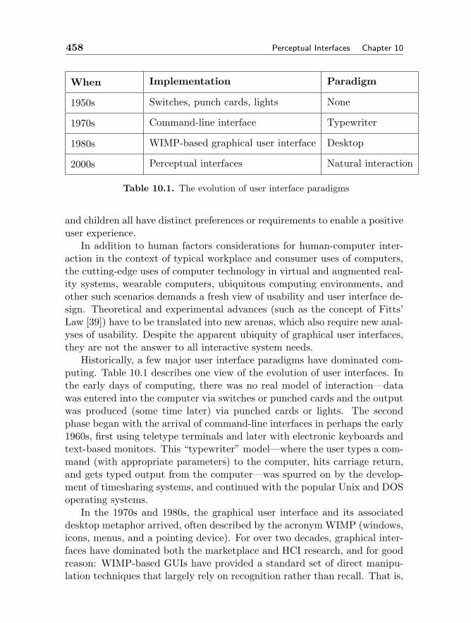
458 Perceptual Interfaces Chapter 10
When Implementation Paradigm
1950s Switches, punch cards, lights None
1970s Command-line interface Typewriter
1980s WIMP-based graphical user interface Desktop
2000s Perceptual interfaces Natural interaction
Table 10.1. The evolution of user interface paradigms
and children all have distinct preferences or requirements to enable a positiveuser experience.
In addition to human factors considerations for human-computer inter-action in the context of typical workplace and consumer uses of computers,the cutting-edge uses of computer technology in virtual and augmented real-ity systems, wearable computers, ubiquitous computing environments, andother such scenarios demands a fresh view of usability and user interface de-sign. Theoretical and experimental advances (such as the concept of Fitts’Law [39]) have to be translated into new arenas, which also require new anal-yses of usability. Despite the apparent ubiquity of graphical user interfaces,they are not the answer to all interactive system needs.
Historically, a few major user interface paradigms have dominated com-puting. Table 10.1 describes one view of the evolution of user interfaces. Inthe early days of computing, there was no real model of interaction—datawas entered into the computer via switches or punched cards and the outputwas produced (some time later) via punched cards or lights. The secondphase began with the arrival of command-line interfaces in perhaps the early1960s, first using teletype terminals and later with electronic keyboards andtext-based monitors. This “typewriter” model—where the user types a com-mand (with appropriate parameters) to the computer, hits carriage return,and gets typed output from the computer—was spurred on by the develop-ment of timesharing systems, and continued with the popular Unix and DOSoperating systems.
In the 1970s and 1980s, the graphical user interface and its associateddesktop metaphor arrived, often described by the acronym WIMP (windows,icons, menus, and a pointing device). For over two decades, graphical inter-faces have dominated both the marketplace and HCI research, and for goodreason: WIMP-based GUIs have provided a standard set of direct manipu-lation techniques that largely rely on recognition rather than recall. That is,
Section 10.2. Perceptual Interfaces and HCI 459
GUI-based commands can typically be easily found and do not have to beremembered or memorized. Direct manipulation is appealing to novice users,it is easy to remember for occasional users, and it can be fast and efficient forfrequent users [124]. Direct manipulation interfaces, in general, allow easylearning and retention, encourage exploration (especially with “Undo” com-mands) and the can give users a sense of accomplishment and responsibilityfor the sequence of actions leading to the completion of a task or subtask.The direct manipulation style of interaction with graphical user interfaceshas been a good match with the office productivity and information accessapplications that have been the “killer apps” of computing to date.
However, as computing changes in terms of physical size and capacity,usage, and ubiquity, the obvious question arises: What is the next majorgeneration in the evolution of user interfaces? Is there a paradigm (and itsassociated technology) that will displace GUI and become the dominant userinterface model? Or will computer interfaces fragment into different modelsfor different tasks and contexts? There is no shortage of HCI research areasbilled as “advanced” or “future” interfaces—these include various flavors ofimmersive environments (virtual, augmented, and mixed reality), 3D inter-faces, tangible interfaces, haptic interfaces, affective computing, ubiquitouscomputing, and multimodal interfaces. These are collectively called “post-WIMP” interfaces by van Dam [138], a general phrase describing interactiontechniques not dependent on classical 2D widgets such as menus and icons.
The (admittedly grandiose) claim of this chapter is that the next domi-nant, long-lasting HCI paradigm is what many people refer to as perceptualinterfaces:
Perceptual User Interfaces (PUIs) are characterized by interaction tech-niques that combine an understanding of natural human capabilities(particularly communication, motor, cognitive, and perceptual skills)with computer I/O devices and machine perception and reasoning.They seek to make the user interface more natural and compelling bytaking advantage of the ways in which people naturally interact witheach other and with the world—both verbal and non-verbal commu-nications. Devices and sensors should be transparent and passive ifpossible, and machines should both perceive relevant human commu-nication channels and generate output that is naturally understood.This is expected to require integration at multiple levels of technolo-gies such as speech and sound recognition and generation, computervision, graphical animation and visualization, language understanding,touch-based sensing and feedback (haptics), learning, user modeling,
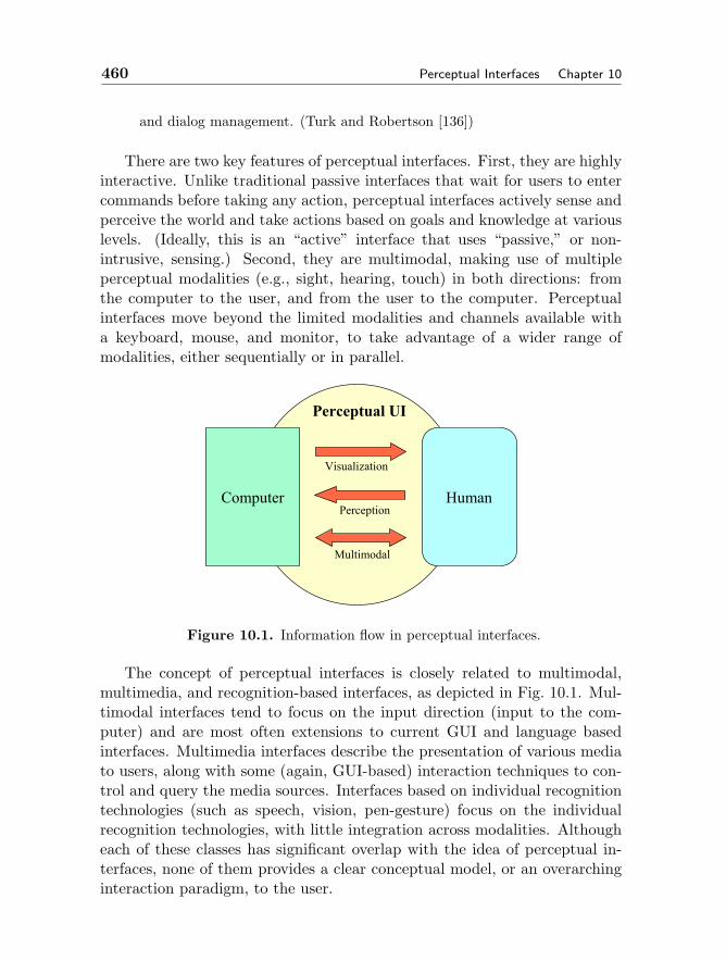
460 Perceptual Interfaces Chapter 10
and dialog management. (Turk and Robertson [136])
There are two key features of perceptual interfaces. First, they are highlyinteractive. Unlike traditional passive interfaces that wait for users to entercommands before taking any action, perceptual interfaces actively sense andperceive the world and take actions based on goals and knowledge at variouslevels. (Ideally, this is an “active” interface that uses “passive,” or non-intrusive, sensing.) Second, they are multimodal, making use of multipleperceptual modalities (e.g., sight, hearing, touch) in both directions: fromthe computer to the user, and from the user to the computer. Perceptualinterfaces move beyond the limited modalities and channels available witha keyboard, mouse, and monitor, to take advantage of a wider range ofmodalities, either sequentially or in parallel.
Perceptual UI
Computer Human
Visualization
Perception
Multimodal
Figure 10.1. Information flow in perceptual interfaces.
The concept of perceptual interfaces is closely related to multimodal,multimedia, and recognition-based interfaces, as depicted in Fig. 10.1. Mul-timodal interfaces tend to focus on the input direction (input to the com-puter) and are most often extensions to current GUI and language basedinterfaces. Multimedia interfaces describe the presentation of various mediato users, along with some (again, GUI-based) interaction techniques to con-trol and query the media sources. Interfaces based on individual recognitiontechnologies (such as speech, vision, pen-gesture) focus on the individualrecognition technologies, with little integration across modalities. Althougheach of these classes has significant overlap with the idea of perceptual in-terfaces, none of them provides a clear conceptual model, or an overarchinginteraction paradigm, to the user.
Section 10.2. Perceptual Interfaces and HCI 461
Sensing/perception Cognitive skills
Social skills Social conventions Shared knowledge
Adaptation
sight sound touch
taste (?) smell (?)
Sensing/perception Cognitive skills
Social skills Social conventions Shared knowledge
Adaptation
vision user modeling
speech
taste (?) smell (?)
haptics
learning graphics
Figure 10.2. Models of interaction: human-human interaction and perceptualhuman-computer interaction.
The general model for perceptual interfaces is that of human-to-humancommunication. While this is not universally accepted in the HCI com-munity as the ultimate interface model (e.g., see [121, 122, 123]), there are

462 Perceptual Interfaces Chapter 10
several practical and intuitive reasons why it makes sense to pursue this goal.Human interaction is natural and in many ways effortless; beyond an earlyage, people do not need to learn special techniques or commands to commu-nicate with one another. There is a richness in human communication viaverbal, visual, and haptic modalities, underscored by shared social conven-tions, shared knowledge, the ability to adapt and to model the other person’spoint of view, that is very different from current computer interfaces, whichessentially implement a precise command-and-control interaction style. Fig-ure 10.2 depicts natural interaction between people and, similarly, betweenhumans and computers. Perceptual interfaces can potentially effect improve-ments in the human factors objectives mentioned earlier in the section, asthey can be easy to learn and efficient to use, they can reduce error rates bygiving users multiple and redundant ways to communicate, and they can bevery satisfying and compelling for users.
People are adaptive in their interactions. Despite an abundance of ambi-guity in natural language, people routinely pursue directions in conversationintended to disambiguate the content of the message. We do the same taskin multiple ways, depending on the circumstances of the moment. A com-puter system that can respond to different modalities or interaction methodsdepending on the context would allow someone to perform a given task withease whether he or she is in the office, in the car, or walking along a noisystreet. Systems that are aware of the user and his or her activities can makeappropriate decisions on how and when to best present information.
A number of studies by Reeves and Nass and their colleagues [96, 109,95] provide compelling evidence that human interaction with computersand other communication technologies is fundamentally social and natural.These studies have produced similar (though typically reduced) social effectsin human-computer interaction as are found in person to person interactions.The general approach to this work has been to choose a social science findingregarding people’s behaviors or attitudes, and to determine if the relevantsocial rule still applies (and to what magnitude) when one of the roles is filledby a computer rather than a human. For example, will users apply do normsof politeness or gender stereotypes to computers? In general, which socialrules will people apply to computers, and how powerful are these rules?
Such studies have found that social responses are automatic and uncon-scious, and can be elicited by basic cues. People show social responses tocues regarding manners and politeness, personality, emotion, gender, trust,ethics, and other social concepts. Much of the research in “social inter-faces” has focused on embodied conversational agents, or lifelike characters,that use speech and language processing to communicate with a human user
Section 10.2. Perceptual Interfaces and HCI 463
[4, 3, 16, 1]. Although the application of these findings is not simple andstraightforward, there are implications for future HCI technologies, and per-ceptual interfaces in particular. An interface that perceives, reasons, and actsin a social manner—even imperfectly—is not too far removed from people’scurrent conceptual models of the technology.
Despite technical advances in speech recognition, speech synthesis, com-puter vision, and artificial intelligence, computers are still, by and large,deaf, dumb, and blind. Many have noted the irony of public restrooms thatare “smarter” than computers because they can sense when people come andgo, and act appropriately, while a computer may wait all night for a user(who has gone home for the evening) to respond to the dialog that asks “Areyou sure you want to do this?” While general purpose machine intelligenceis still a difficult and elusive goal, our belief is that much can be gained bypursuing an agenda of technologies to support the human-to-human modelof interaction. Even if the Holy Grail of perceptual interfaces is far in thefuture, the near-term benefits may be transformational, as component tech-nologies and integration techniques mature and provide new tools to improvethe ways in which people interact with technology.
In addition to the general goal of interfaces that better match human ca-pabilities and provide a more natural and compelling user experience, thereare immediate application areas that are ripe for early perceptual interfacetechnologies. The computer game industry is particularlly compelling, as itis large and its population of users tend to be early adopters of new technolo-gies. Game interfaces that can perceive the user’s identity, body movement,and speech, for example, are likely to become very popular. Another groupof people who may have a lot to gain from early perceptual interfaces areusers with physical disabilities. Interfaces that are more adaptable and flex-ible, and not limited to particular ways of moving a mouse or typing keys,will provide a significant benefit to this community.
Several other areas—such as entertainment, personal robotics, multime-dia learning, and biometrics—would clearly seem to benefit from initial ad-vances in perceptual interfaces. Eventually, the applications of technologiesand sense, perceive, understand, and respond appropriately to human be-havior appear to be unlimited.
What is necessary in order to bring about this vision of perceptual inter-faces? A better understanding of human capabilities, limitations, and pref-erences in interaction is important, including physical, social, and cognitiveaspects. Advances in several technical areas, some quite old and some rela-tively new, are also vital. Speech understanding and generation (i.e., speechrecognition, natural language processing, speech synthesis, discourse mod-
464 Perceptual Interfaces Chapter 10
eling, and dialogue management) are vital to leverage the natural modalityof spoken language, as well as other sound recognition and synthesis tools(e.g., in addition to words, systems should recognize a sneeze, a cough, aloud plane passing overhead, a general noisy environment, etc.). Computergraphics and information visualization are important to provide richer waysof communicating to users. Affective computing [105] may be vital to un-derstand and generate natural interaction, especially subtle cues to aspectsof humor and irony, and appropriate context-dependent displays of emo-tion (or lack thereof). Haptic and tangible interfaces (e.g., [7, 57]) whichleverage physical aspects of interaction may also be important in buildingtruly perceptual interfaces. User and task modeling (e.g., [52, 53]) is key tounderstanding the whole context of interaction.
Computer vision is also a vital element of perceptual interfaces. Whetheralone or in conjunction with other perceptual modalities, visual informationprovides useful and important cues to interaction. The presence, location,and posture of a user may be important contextual information; a gestureor facial expression may be a key signal; the direction of gaze may disam-biguate the object referred to in language as “this” or “that thing.” Thenext section of the chapter describes the scope of computer vision researchand development as it relates to this area of perceptual interfaces.
In addition to advances in individual component areas, the integrationof multiple modalities is of fundamental importance in perceptual interfaces.Both lower-level fusion techniques and higher-level integration frameworkswill be necessary to build interactive, multimodal interfaces that provide acompelling, natural user experience.
10.3 Multimodal Interfaces
A multimodal interface is a system that combines two or more input modal-ities in a coordinated manner. Perceptual interfaces are inherently multi-modal. In this section, we define more precisely what we mean by modesand channels, and discuss research in multimodal interfaces and how thisrelates to the more general concept of perceptual interfaces.
Humans interact with the world by way of information being sent andreceived, primarily through the five major senses of sight, hearing, touch,taste, and smell. A modality (informally, a mode) refers to a particularsense. A communication channel is a course or pathway through which in-formation is transmitted. In typical HCI usage, a channel describes the inter-action technique that utilizes a particular combination of user and computercommunication—i.e., the user output/computer input pair or the computer
Section 10.3. Multimodal Interfaces 465
output/user input pair1. This can be based on a particular device, such asthe keyboard channel or the mouse channel, or on a particular action, suchas spoken language, written language, or dynamic gestures. In this view,the following are all channels: text (which may use multiple modalities whentyping in text or reading text on a monitor), sound, speech recognition,images/video, and mouse pointing and clicking.
Unfortunately, there is some ambiguity in the use of the word mode inHCI circles, as sometimes it is used to mean “modality” and at other times itmeans “channel.” So are multimodal interfaces “multi-modality” or “multi-channel?” Certainly every command line interface uses multiple modalities,as sight and touch (and sometimes sound) are vital to these systems. Thesame is true for graphical user interfaces, which in addition use multiplechannels of keyboard text entry, mouse pointing and clicking, sound, images,etc.
What then distinguishes multimodal interfaces from other HCI technolo-gies? As a research field, multimodal interfaces focus on integrating sensorrecognition-based input technologies such as speech recognition, pen gesturerecognition, and computer vision, into the user interface. The function ofeach technology is better thought of as a channel than as a sensing modal-ity; hence, in our view, a multimodal interface is one that uses multiplemodalities to implement multiple channels of communication. Using multi-ple modalities to produce a single interface channel (e.g., vision and sound toproduce 3D user location) is multisensor fusion, not a multimodal interface.Similarly, using a single modality to produce multiple channels (e.g., a left-hand mouse to navigate and a right-hand mouse to select) is a multichannel(or multi-device) interface, not a multimodal interface.
An early prototypical multimodal interfaces was the “Put That There”prototype system demonstrated at MIT in the early 1980s [10]. In this sys-tem, the user communicated via speech and pointing gestures in a “mediaroom.” The gestures served to disambiguate the speech (Which object doesthe word “this” refer to? What location is meant by “there?”) and effectedother direct interactions with the system. More recently, the QuickSet ar-chitecture [18] is a good example of a multimodal system using speech andpen-based gesture to interact with map-based and 3D visualization systems.QuickSet is a wireless, handheld, agent-based, collaborative multimodal sys-tem for interacting with distributed applications. The system analyzes con-tinuous speech and pen gesture in real time and produces a joint semanticinterpretation using a statistical unification-based approach. The system
1Input means to the computer; output means from the computer.

466 Perceptual Interfaces Chapter 10
supports unimodal speech or gesture as well as multimodal input.Multimodal systems and architectures vary along several key dimensions
or characteristics, including:
– The number and type of input modalities;– The number and type of communication channels;– Ability to use modes in parallel, serially, or both;– The size and type of recognition vocabularies;– The methods of sensor and channel integration;– The kinds of applications supported.
There are many potential advantages of multimodal interfaces, includingthe following [101]:
– They permit the flexible use of input modes, including alternation andintegrated use.
– They support improved efficiency, especially when manipulating graph-ical information.
– They can support shorter and simpler speech utterances than a speech-only interface, which results in fewer disfluencies and more robustspeech recognition.
– They can support greater precision of spatial information than a speech-only interface, since pen input can be quite precise.
– They give users alternatives in their interaction techniques.– They lead to enhanced error avoidance and ease of error resolution.– They accommodate a wider range of users, tasks, and environmental
situations.– They are adaptable during continuously changing environmental con-
ditions.– They accommodate individual differences, such as permanent or tem-
porary handicaps.– They can help prevent overuse of any individual mode during extended
computer usage.
Oviatt and Cohen and their colleagues at the Oregon Health and ScienceUniversity (formerly Oregon Graduate Institute) have been at the forefrontof multimodal interface research, building and analyzing multimodal systemsover a number of years for a variety of applications. Oviatt’s “Ten Mythsof Multimodal Interaction” [100] are enlightening for anyone trying to un-derstand the area. We list Oviatt’s myths in italics, with our accompanyingcomments:

Section 10.3. Multimodal Interfaces 467
Myth #1. If you build a multimodal system, users will interact multi-modally. In fact, users tend to intermix unimodal and multimodalinteractions; multimodal interactions are often predictable based onthe type of action being performed.
Myth #2. Speech and pointing is the dominant multimodal integration pat-tern. This is only one of many interaction combinations, comprisingperhaps 14all spontaneous multimodal utterances.
Myth #3. Multimodal input involves simultaneous signals. Multimodalsignals often do not co-occur temporally.
Myth #4. Speech is the primary input mode in any multimodal system thatincludes it. Speech is not the exclusive carrier of important content inmultimodal systems, nor does it necessarily have temporal precedenceover other input modes.
Myth #5. Multimodal language does not differ linguistically from unimodallanguage. Multimodal language is different, and often much simplified,compared with unimodal language.
Myth #6. Multimodal integration involves redundancy of content betweenmodes. Complementarity of content is probably more significant inmultimodal systems than is redundancy.
Myth #7. Individual error-prone recognition technologies combine multi-modally to produce even greater unreliability. In a flexible multimodalinterface, people figure out how to use the available input modes effec-tively; in addition, there can be mutual disambiguation of signals thatalso contributes to a higher level of robustness.
Myth #8. All users’ multimodal commands are integrated in a uniformway. Different users may have different dominant integration patterns.
Myth #9. Different input modes are capable of transmitting comparablecontent. Different modes vary in the type and content of their infor-mation, their functionality, the ways they are integrated, and in theirsuitability for multimodal integration.
Myth #10. Enhanced efficiency is the main advantage of multimodal sys-tems. While multimodal systems may increase efficiency, this may notalways be the case. The advantages may reside elsewhere, such asdecreased errors, increased flexibility, or increased user satisfaction.

468 Perceptual Interfaces Chapter 10
A technical key to multimodal interfaces is the specific integration levelsand technique(s) used. Integration of multiple sources of information is gen-erally characterized as “early,” “late,” or somewhere in between. In earlyintegration (or “feature fusion”), the raw data from multiple sources (ordata that has been processed somewhat, perhaps into component features)are combined and recognition or classification proceeds in the multidimen-sional space. In late integration (or “semantic fusion”), individual sensorchannels are processed through some level of classification before the resultsare integrated. Figure 10.3 shows a view of these alternatives. In practice,integration schemes may combine elements of early and late integration, oreven do both in parallel.
Sensor 1
Sensor 2
Featurespace
Classification Output
(a)
Sensor 1
Sensor 2
Classification
OutputFeaturespace
Classification
(b)
Figure 10.3. (a) Early integration, fusion at the feature level. (b) Late integration,fusion at the semantic level.
There are advantages to using late, semantic integration of multiplemodalities in multimodal systems. For example, the input types can berecognized independently, and therefore do not have to occur simultane-ously. The training requirements are smaller, O(2N) for two separatelytrained modes as opposed to O(N2) for two modes trained together. Thesoftware development process is also simpler in the late integration case, as

Section 10.3. Multimodal Interfaces 469
exemplified by the QuickSet architecture [148]. Quickset uses temporal andsemantic filtering, unification as the fundamental integration technique, anda statistical ranking to decide among multiple consistent interpretations.
Multimodal interface systems have used a number of non-traditionalmodes and technologies. Some of the most common are the following:
– Speech recognition
Speech recognition has a long history of research and commercial de-ployment, and has been a popular component of multimodal systemsfor obvious reasons. Speech is a very important and flexible commu-nication modality for humans, and is much more natural than typingor any other way of expressing particular words, phrases, and longerutterances. Despite the decades of research in speech recognition andover a decade of commercially available speech recognition products,the technology is still far from perfect, due to the size, complexity,and subtlety of language, the limitations of microphone technology,the plethora of disfluencies in natural speech, and problems of noisyenvironments. Systems using speech recognition have to be able torecover from the inevitable errors produced by the system.
– Language understanding
Natural language processing attempts to model and understand hu-man language, whether spoken or written. In multimodal interfaces,language understanding may be hand-in-hand with speech recognition(together forming a “speech understanding” component), or it may beseparate, processing the user’s typed or handwritten input. Typicallythe more a system incorporates natural language, the more users willexpect sophisticated semantic understanding from the system. Currentsystems are unable to deal with completely unconstrained language,but can do quite well with limited vocabularies and subject matter.Allowing for user feedback to clarify and disambiguate language inputcan help language understanding systems significantly.
– Pen-based gesture
Pen-based gesture has been popular in part because of computer formfactors (PDAs and tablet computers) that include a pen or stylus asa primary input device. Pen input is particularly useful for deictic(pointing) gestures, defining lines, contours, and areas, and specially-defined gesture commands (e.g., minimizing a window by drawing alarge “M” on the screen). Pen-based systems are quite useful in mobile
470 Perceptual Interfaces Chapter 10
computing, where a small computer can be carried, but a keyboard isimpractical.
– Magnetic, inertial, etc. sensors for body tracking
Sturman’s 1991 thesis [131] thoroughly documented the early use ofsensors worn on the hand for input to interactive systems. Magnetictracking sensors such as the Ascension Flock of Birds2 product, vari-ous instrumented gloves, and sensor- or marker-based motion capturedevices have been used in multimodal interfaces, particularly in im-mersive environments (e.g., see [50]).
– Non-speech sound
Non-speech sounds have traditionally been used in HCI to providesignals to the user: e.g., warnings, alarms, and status information.(Ironically, one of the most useful sounds for computer users is ratherserendipitous: the noise made by many hard drives that lets a userknow that the machine is still computing, rather than hung.) However,non-speech sound can also be a useful input channel, as sound made byusers can be meaningful events in human-to-human communication—e.g., utterances such as “uh-huh” used in backchannel communication(communication events that occur in the background of an interaction,rather than being the main focus), a laugh, a sigh, or a clapping ofhands.
– Haptic input and force feedback
Haptic, or touch-based, input devices measure pressure, velocity, location—essentially perceiving aspects of a user’s manipulative and explorativemanual actions. These can be integrated into existing devices (e.g.,keyboards and mice that know when they are being touched, and pos-sibly by whom). Or they can exist as standalone devices, such as thewell-known PHANTOM device by SensAble Technologies, Inc.3 (seeFig. 10.4), or the DELTA device by Force Dimension.4 These and mostother haptic devices integrate force feedback and allow the user to expe-rience the “touch and feel” of simulated artifacts as if they were real.Through the mediator of a hand-held stylus or probe, haptic explo-ration can now receive simulated feedback including rigid boundaries
2http://www.ascension-tech.com3http://www.sensable.com4http://www.forcedimension.com
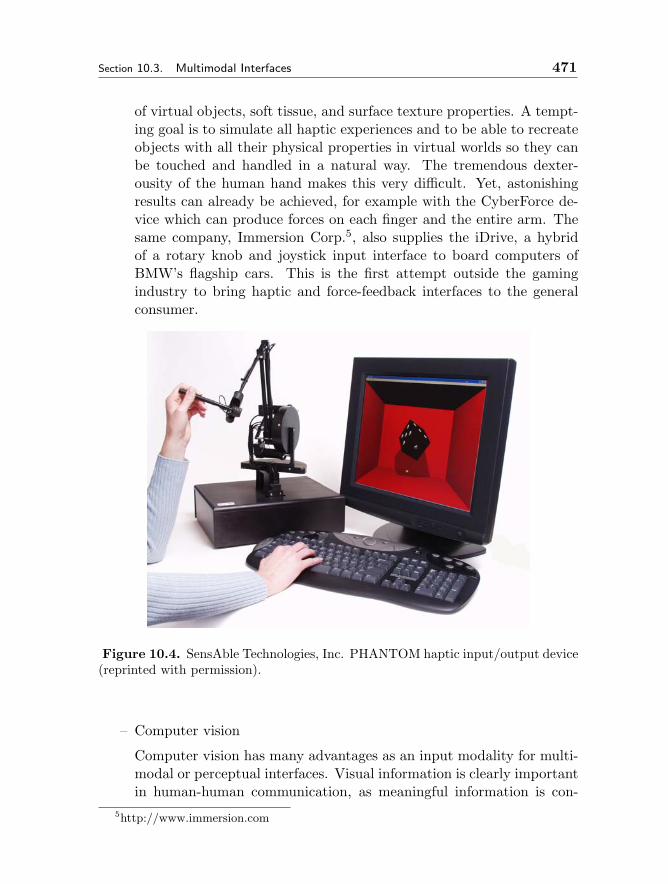
Section 10.3. Multimodal Interfaces 471
of virtual objects, soft tissue, and surface texture properties. A tempt-ing goal is to simulate all haptic experiences and to be able to recreateobjects with all their physical properties in virtual worlds so they canbe touched and handled in a natural way. The tremendous dexter-ousity of the human hand makes this very difficult. Yet, astonishingresults can already be achieved, for example with the CyberForce de-vice which can produce forces on each finger and the entire arm. Thesame company, Immersion Corp.5, also supplies the iDrive, a hybridof a rotary knob and joystick input interface to board computers ofBMW’s flagship cars. This is the first attempt outside the gamingindustry to bring haptic and force-feedback interfaces to the generalconsumer.
Figure 10.4. SensAble Technologies, Inc. PHANTOM haptic input/output device(reprinted with permission).
– Computer vision
Computer vision has many advantages as an input modality for multi-modal or perceptual interfaces. Visual information is clearly importantin human-human communication, as meaningful information is con-
5http://www.immersion.com
472 Perceptual Interfaces Chapter 10
veyed through identity, facial expression, posture, gestures, and othervisually observable cues. Sensing and perceiving these visual cues fromvideo cameras appropriately placed in the environment is the domainof computer vision. The following section describes relevant computervision technologies in more detail.
10.4 Vision Based Interfaces
Vision supports a wide range of human tasks, including recognition, navi-gation, balance, reading, and communication. In the context of perceptualinterfaces, the primary task of computer vision (CV) is to detect and rec-ognize meaningful visual cues to communication—i.e., to “watch the users”and report on their locations, expressions, gestures, etc. While vision is oneof possibly several sources of information about the interaction to be com-bined multimodally in a perceptual interface, in this section we focus solelyon the vision modality. Using computer vision to sense and perceive the userin an HCI context is often referred to as Vision Based Interaction, or VisionBased Interfaces (VBI).
In order to accurately model human interaction, it is necessary to takeevery observable behavior into account [69, 68]. The analysis of humanmovement and gesture coordinated with speech conversations has a longhistory in areas such as sociology, communication, and therapy (e.g., Scheflenand Birdwhistell’s Context Analysis [115]). These analyses, however, areoften quite subjective and ill-suited for computational analysis. VBI aimsto produce precise and real-time analysis that will be useful in a wide rangeof applications, from communication to games to automatic annotation ofhuman-human interaction.
There is a range of human activity that has occupied VBI research overthe past decade; Fig. 10.5 shows some of these from the camera’s viewpoint.Key aspects of VBI include the detection and recognition of the followingelements:
– Presence and location – Is someone there? How many people? Whereare they (in 2D or 3D)? [Face detection, body detection, head andbody tracking]
– Identity – Who are they? [Face recognition, gait recognition]– Expression – Is a person smiling, frowning, laughing, speaking...? [Fa-
cial feature tracking, expression modeling and analysis]– Focus of attention – Where is a person looking? [Head/face tracking,
eye gaze tracking]
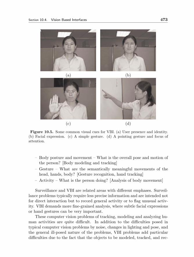
Section 10.4. Vision Based Interfaces 473
(a) (b)
(c) (d)
Figure 10.5. Some common visual cues for VBI. (a) User presence and identity.(b) Facial expression. (c) A simple gesture. (d) A pointing gesture and focus ofattention.
– Body posture and movement – What is the overall pose and motion ofthe person? [Body modeling and tracking]
– Gesture – What are the semantically meaningful movements of thehead, hands, body? [Gesture recognition, hand tracking]
– Activity – What is the person doing? [Analysis of body movement]
Surveillance and VBI are related areas with different emphases. Surveil-lance problems typically require less precise information and are intended notfor direct interaction but to record general activity or to flag unusual activ-ity. VBI demands more fine-grained analysis, where subtle facial expressionsor hand gestures can be very important.
These computer vision problems of tracking, modeling and analyzing hu-man activities are quite difficult. In addition to the difficulties posed intypical computer vision problems by noise, changes in lighting and pose, andthe general ill-posed nature of the problems, VBI problems add particulardifficulties due to the fact that the objects to be modeled, tracked, and rec-
474 Perceptual Interfaces Chapter 10
ognized are people, rather than simple, rigid, non-changing widgets. Peoplechange hairstyles, get sunburned, grow facial hair, wear baggy clothing, andin general make life difficult for computer vision algorithms. Robustness inthe face of the variety of human appearances is a major issue in VBI research.
The main problem that computer vision faces is an overload of informa-tion. The human visual system effortlessly filters out unimportant visualinformation, attending to relevant details like fast moving objects, even ifthey are in the periphery of the visible hemisphere. But this is a very com-plex computational task. At the low level in human vision, a great dealof pre-processing is done in the retina in order to decrease the bandwidthrequirements of the nervous channel into the visual cortex. At the highlevel, humans leverage a priori knowledge of the world in ways that are notwell understood computationally. For example, a computer does not simplyknow that objects under direct sunlight cast sharp shadows. The difficultquestion is how to extract only relevant observations from the visual infor-mation so that vision algorithms can concentrate on a manageable amount ofwork. Researchers frequently circumvent this problem by making simplify-ing assumptions about the environment, which makes it possible to developworking systems and investigate the suitability of computer vision as a userinterface modality.
In recent years, there has been increased interest in developing practicalvision-based interaction methods. The technology is readily available, inex-pensive, and fast enough for most real-time interaction tasks. CPU speed hascontinually increased following Moore’s Law, allowing increasingly complexvision algorithms to run at frame rate (30 frames per second, fps). Fig-ure 10.6 shows a history of available clock cycles per pixel of a VGA-sizedvideo stream with a top-of-the-line CPU for the PC market over the last 35years. Higher processing speeds, as well as the recent boom in digital imagingin the consumer market, could have far reaching implications for VBI. It isbecoming more and more feasible to process large, high resolution images innear real-time, potentially opening the door for numerous new applicationsand vision algorithms.
Fast, high-resolution digital image acquisition devices and fast processingpower are only as effective as the link between them. The PC market hasjust recently seen a revolution in connector standards. Interface speeds toperipheral devices used to be orders of magnitude lower than the connectionspeed between the motherboard and internal devices. This was largely dueto the parallel (32 bit or more) connector structure for internal boards andserial links to external devices. The introduction of Firewire (also called 1394and i-Link) in 1995 and more recently USB 2.0 pushed interface speeds for
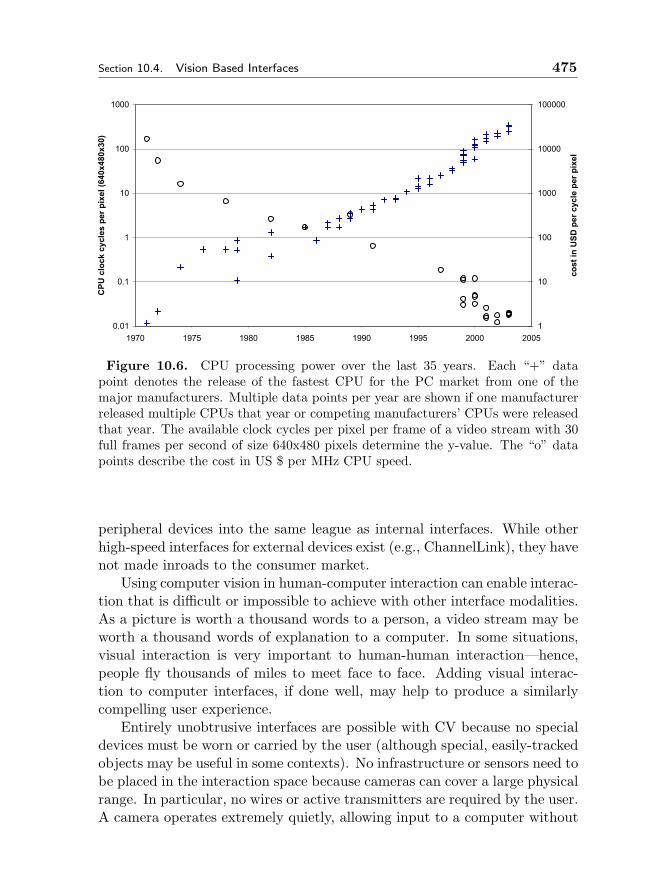
Section 10.4. Vision Based Interfaces 475
0.01
0.1
1
10
100
1000
1970 1975 1980 1985 1990 1995 2000 2005
CP
U c
lock
cyc
les
per
pix
el (
640x
480x
30)
1
10
100
1000
10000
100000
cost
in
US
D p
er c
ycle
per
pix
el
Figure 10.6. CPU processing power over the last 35 years. Each “+” datapoint denotes the release of the fastest CPU for the PC market from one of themajor manufacturers. Multiple data points per year are shown if one manufacturerreleased multiple CPUs that year or competing manufacturers’ CPUs were releasedthat year. The available clock cycles per pixel per frame of a video stream with 30full frames per second of size 640x480 pixels determine the y-value. The “o” datapoints describe the cost in US $ per MHz CPU speed.
peripheral devices into the same league as internal interfaces. While otherhigh-speed interfaces for external devices exist (e.g., ChannelLink), they havenot made inroads to the consumer market.
Using computer vision in human-computer interaction can enable interac-tion that is difficult or impossible to achieve with other interface modalities.As a picture is worth a thousand words to a person, a video stream may beworth a thousand words of explanation to a computer. In some situations,visual interaction is very important to human-human interaction—hence,people fly thousands of miles to meet face to face. Adding visual interac-tion to computer interfaces, if done well, may help to produce a similarlycompelling user experience.
Entirely unobtrusive interfaces are possible with CV because no specialdevices must be worn or carried by the user (although special, easily-trackedobjects may be useful in some contexts). No infrastructure or sensors need tobe placed in the interaction space because cameras can cover a large physicalrange. In particular, no wires or active transmitters are required by the user.A camera operates extremely quietly, allowing input to a computer without
476 Perceptual Interfaces Chapter 10
disturbing the environment. Also, modern cameras can be very lightweightand compact, well-suited for mobile applications. Even in environmentsunsuitable for moving or exposed parts, cameras can be utilized since acamera can be completely encapsulated in its housing with a transparentwindow.
The cost of cameras and their supporting hardware and software hasdropped dramatically in recent years, making it feasible to expect a largeinstalled based in the near future. Software for image and video processing(e.g., for movie and DVD editing) has entered the consumer market and isfrequently pre-installed, bundled with a computer’s operating system.
The versatility of a camera makes it reasonable and compelling to use asan interface device. A camera may be used for several different purposes,sometimes simultaneously. For example, a single camera, affixed to a per-son’s head or body, may function as a user interface device by observingthe wearer’s hands [73]; it can videotape important conversations or othervisual memories at the user’s request [58]; it can store and recall the facesof conversation partners and associate their names [112]; it can be used totrack the user’s head orientation [140, 2]; it can guide a museum visitor byidentifying and explaining paintings [111].
As a particular example of VBI, hand gesture recognition offers manypromising approaches for interaction. Hands can operate without obstruct-ing high-level activities of the brain such as sentence-forming, thus beinga good tool for interface tasks while thinking. Generating speech, on theother hand, is said to take up general-purpose brain resources, impedingthe thought process [66]. Hands are very dextrous physical tools, and theircapabilities have been quite successfully employed in the HCI context in con-junction with devices such as the keyboard and mouse. Human motor skillsare, in many cases, easily trained to execute new tasks with high precisionand incredible speeds. With the aid of computer vision, we have the chanceto go beyond the range of activities that simple physical devices can captureand instead to let hands gesture with all their capabilities. The goal is toleverage the full range of both static hand postures and dynamic gestures inorder to communicate (purposefully or otherwise) and perhaps to commandand control. Data gloves accomplish some of this goal, yet they have anunnatural feel and are cumbersome to the user.
10.4.1 Terminology
This subsection reviews the essential terminology relevant to vision basedinteraction. Current VBI tasks focus on modeling (and detecting, tracking,
Section 10.4. Vision Based Interfaces 477
recognizing, etc.) one or more body parts. These parts could be a face,a hand, a facial feature such as an eye, or an entire body. We will inter-changeably call this the object of focus, the feature of attention, or simplythe “body part.”
Determining the presence (or absence) of an object of focus is the problemof detection and has so far primarily been applied to people detection [43]and face detection [155, 49]. Strictly speaking, the output is binary (“personpresent” versus “no person present”), but typically the location of the objectis also reported. Object localization is sometimes used to describe the specialcase that the presence of an object is assumed and its location is to bedetermined at a particular point in time. Registration refers to the problem ofaligning an object model to the observation data, often both object positionand orientation (or pose). Object tracking locates objects and reports theirchanging pose over time [43].
Although tracking can be considered as a repeated frame-by-frame de-tection or localization of a feature or object, it usually implies more thandiscontinuous processing. Various methods improve tracking by explicitlytaking temporal continuity into account and using prediction to limit thespace of possible solutions and speed up the processing. One general ap-proach uses filters to model the object’s temporal progression. This can beas simple as linear smoothing, which essentially models the object’s inertia.A Kalman filter [63] assumes a Gaussian distribution of the motion pro-cess and can thus also model non-constant movements. The frequently usedExtended Kalman Filter (EKF) relieves the necessity of linearity. Particlefiltering methods (or sequential Monte Carlo methods [34], and frequentlycalled Condensation [55] in the vision community) make no assumptionsabout the characteristics of underlying probability distributions but insteadsample the probability and build an implicit representation. They can there-fore deal with non-Gaussian processes and also with multi-modal densities(caused by multiple, statistically independent sources) such as arise fromobject tracking in front of cluttered backgrounds. In addition to the filter-ing approach, different algorithms can be used for initialization (detection)and subsequent tracking. For example, some approaches detect faces with alearning-based approach [139] and then track with a shape and color basedhead tracker [8].
Recognition (or identification) involves comparing an input image to aset of models in a database. A recognition scheme usually determines con-fidence scores or probabilities that defines how closely the image data fitseach model. Detection is sometimes called recognition, which makes senseif there are very different classes of objects (faces, cars, and books) and one
478 Perceptual Interfaces Chapter 10
of them (faces) must be recognized. A special case of recognition is verifica-tion or authentication, which judges whether the input data belongs to oneparticular identity with very high confidence. An important application ofverification is in biometrics, which has been applied to faces, fingerprints,and gait characteristics [17].
A posture is a static configuration of the human body—for example, sit-ting and thinking or holding a coffee cup or pen. Gestures are dynamicmotions of the body or body parts, and can be considered as temporallyconsecutive sequences of postures. Hand and arm gestures in particular arecovered extensively in the social sciences literature, especially in conversa-tional and behavioral psychology [36, 69, 86, 87, 108]. As a result, the termgesture is often used to refer to the semantic interpretation that is asso-ciated with a particular movement of the body (e.g., happiness associatedwith a smile). We limit our attention in this chapter to a mostly syntacticview of “gesture” and “gesture recognition,” leaving the difficult problem ofsemantic interpretation and context [26, 86] to others.
Facial gestures are more commonly called facial expressions. Detectingand tracking facial features are typically the first steps of facial expressionanalysis, although holistic appearance-based approaches may also be feasible.Subsequent steps try to recognize known expressions (e.g., via FACS actionunits [37]) and to infer some meaning from them, such as the emotional stateof the human [6, 9].
The parameter set for a rigid body consists of its location (x, y, z) in3D space and its orientation (rx, ry, rz) with respect to a fixed coordinateframe. Deformable objects such as human faces require many parametersfor an accurate description of their form, as do articulated objects such ashuman bodies. An object’s appearance describes its color and brightnessproperties at every point on its surface. Appearance is caused by texture,surface structure, lighting, and view direction. Since these attributes areview-dependent, it only makes sense to talk about appearance from a givenviewpoint.
The view sphere is an imaginary sphere around the object or scene of in-terest. Every surface point of the sphere defines a different view of the object.When taking perspective into account, the object’s appearance changes evenfor different distances, despite a constant viewing angle. Vision techniquesthat can detect, track, or recognize an object regardless of the viewing angleare called view-independent; those that require a certain range of viewingangles for good performance, for example frontal views for face tracking, arecalled view-dependent.
Section 10.4. Vision Based Interfaces 479
10.4.2 Elements of VBI
VBI techniques apply computer vision to specific body parts and objects ofinterest. Depending on the application and environmental factors, it maybe most useful to search for or track the body as a whole, individual limbs,a single hand, or an artifact such as a colored stick held by the user. VBItechniques for different body parts and features can complement and aideach other in a number of ways.
1. Coarse-to-fine hierarchy: Here, in a sequence of trackers which aretargeted to successively more detailed objects, each stage benefits fromthe results of the previous stage by drastically reducing the searchspace. For example, whole-body detection limits the search space forface detection. After the face is detected in a scene, the search forparticular facial features such as eyes can be limited to small areaswithin the face. After the eyes are identified, one might estimate theeye gaze direction [129].
2. Fine-to-coarse hierarchy: This approach works in the opposite way.From a large number of cues of potential locations of small features,the most likely location of a larger object that contains these featuresis deduced. For example, feature-based face recognition methods makeuse of this approach. They first try to identify prominent featuressuch as eyes, nose, and lips in the image. This may yield many falsepositives, but knowledge about the features’ relative locations allowsthe face to be detected. Bodies are usually attached to heads at thesame location: thus, given the position of a face, the search for limbs,hands, etc., becomes much more constrained and therefore simpler [91].
3. Assistance through more knowledge: The more elements in a scenethat are modeled, the easier it is to deal with their interactions. Forexample, if a head tracking interface also tracks the hands in the image,although it does not need their locations directly, it can account forocclusions of the head by the hands (e.g., [146]). The event is withinits modeled realm, whereas otherwise occlusions would constitute anunanticipated event, diminishing the robustness of the head tracker.
Face tracking in particular is often considered a good anchor point forother objects [135, 24], since faces can be fairly reliably detected based onskin color or frontal view appearance.

480 Perceptual Interfaces Chapter 10
Person-level, Whole Body & Limb Tracking
VBI at the person-level has probably produced the most commercial appli-cations to date. Basic motion sensing is a perfect example how effective VBIcan be in a constrained setting: the scene is entirely stationary, so that frame-to-frame differencing is able to detect moving objects. Another successfulapplication is in traffic surveillance and control. A number of manufactur-ers offer systems that automate or augment the push button for pedestriancrossings. The effectiveness of this technology was demonstrated in a study[137] that compared the number of people crossing an intersection during the“Don’t Walk” signal with and without infrastructure that detected peoplein the waiting area on the curb or in the crossing. The study found that inall cases these systems can significantly decrease the number of dangerousencounters between people and cars.
Motion capture has frequently been used in the film industry to animatecharacters with technology from companies such as Adtech, eMotion, Mo-tion Analysis, and Vicon Motion Systems. In optical motion capture, manyIR-reflecting markers are placed on an artist’s or actor’s body. Typicallymore than five cameras observe the acting space from different angles, sothat at least two cameras can see each point at any time. This allows forprecise reconstruction of the motion trajectories of the markers in 3D andeventually the exact motions of the human body. This information is usedto drive animated models and can result in much more natural motions thanthose generated automatically. Other common applications of motion cap-ture technology include medical analysis and sports training (e.g., to analyzegolf swings or tennis serves).
Detecting and tracking people passively using computer vision, withoutthe use of markers, has been applied to motion detection and other surveil-lance tasks. In combination with artificial intelligence, it is also possible todetect unusual behavior, for example in the context of parking lot activityanalysis [47]. Some digital cameras installed in classrooms and auditori-ums are capable of following a manually selected person or head throughpan-tilt-zoom image adjustments. Object-based image encoding such as de-fined in the MPEG-4 standard is an important application of body trackingtechnologies.
The difficulties of body tracking arise from the many degrees of freedomof the human body. Adults have 206 bones which are connected by over230 joints. Ball and socket joints such as in the shoulder and hip have threedegrees of freedom (DOF): They can abduct and adduct, flex and extend,and rotate around the limb’s longitudinal axis. Hinge joints have one DOF
Section 10.4. Vision Based Interfaces 481
and are found in the elbow and between the phalanges of hands and feet.Pivot joints also allow for one DOF; they allow the head as well as radiusand ulna to rotate. The joint type in the knee is called a condylar joint.It has two DOF because it allows for flexion and extension and for a smallamount of rotation. Ellipsoid joints also have two DOF, one for flexion andextension, the other for abduction and adduction (e.g., the wrist’s main jointand the metacarpophalangeal joint as depicted in Fig. 10.8). The thumb’sjoint is a unique type, called a saddle joint; in addition to the two DOFof ellipsoid joints, it also permits a limited amount of rotation. The jointsbetween the human vertebrae each allow limited three DOF motion, and alltogether they are responsible for the trunk’s flexibility.
Recovering the degrees of freedom for all these joints is an impossible featfor today’s vision technology. Body models for CV purposes must thereforeabstract from this complexity. They can be classified by their dimensionalityand by the amount of knowledge versus learning needed to construct them.
The frequently used 3D kinematic models have between 20 and 30 DOF.Figure 10.7 shows an example, in which the two single-DOF elbow- andradioulnar joints have been combined into a two-DOF joint at the elbow. Infact, the rotational DOF of the shoulder joint is often transferred to the elbowjoint. This is because the humerus shows little evidence of its rotation, whilethe flexed lower arm indicates this much better. Similarly, the rotationalDOF of the radioulnar joint can be attributed to the wrist. This transfermakes a hierarchical model parameter estimation easier.
Most of the vision-based efforts to date have concentrated on detectingand tracking people while walking, dancing, or performing other tasks in amostly upright posture. Pedestrian detection, for example, has seen meth-ods employed that had previously shown success in face detection, such aswavelets [99] and a combination of depth information and a learning method[162].
Two systems with comprehensive functionality, Pfinder [145] and W4[48], both show well how CV must be tailored to the task and properties of theparticular environment. First, they rely on a static camera mounting, whichgives the opportunity to model the background and achieve fast and reliablesegmentation of moving foreground objects. Second, they make assumptionsof the body posture; namely, they expect a mostly upright person. This canbe easily distinguished from other moving objects such as cars or wind-blownobjects. Third, heuristics about the silhouettes enable classification of a fewtypical postures or actions such as carrying an object, making use of the factthat only a small number of scenarios are likely for a person entering thefield of view.
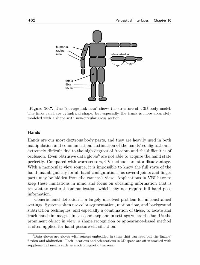
482 Perceptual Interfaces Chapter 10
3 3
3
33 2 1
2
1
1 1
1 1
2
often modeled as:
2 2 2
humerusradiusulna
femurtibiafibula
11
Figure 10.7. The “sausage link man” shows the structure of a 3D body model.The links can have cylindrical shape, but especially the trunk is more accuratelymodeled with a shape with non-circular cross section.
Hands
Hands are our most dextrous body parts, and they are heavily used in bothmanipulation and communication. Estimation of the hands’ configuration isextremely difficult due to the high degrees of freedom and the difficulties ofocclusion. Even obtrusive data gloves6 are not able to acquire the hand stateperfectly. Compared with worn sensors, CV methods are at a disadvantage.With a monocular view source, it is impossible to know the full state of thehand unambiguously for all hand configurations, as several joints and fingerparts may be hidden from the camera’s view. Applications in VBI have tokeep these limitations in mind and focus on obtaining information that isrelevant to gestural communication, which may not require full hand poseinformation.
Generic hand detection is a largely unsolved problem for unconstrainedsettings. Systems often use color segmentation, motion flow, and backgroundsubtraction techniques, and especially a combination of these, to locate andtrack hands in images. In a second step and in settings where the hand is theprominent object in view, a shape recognition or appearance-based methodis often applied for hand posture classification.
6Data gloves are gloves with sensors embedded in them that can read out the fingers’flexion and abduction. Their locations and orientations in 3D space are often tracked withsupplemental means such as electromagnetic trackers.
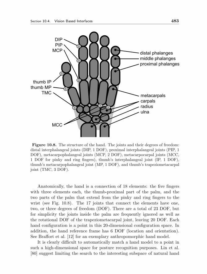
Section 10.4. Vision Based Interfaces 483
distal phalangesmiddle phalangesproximal phalanges
DIPPIP
MCP
metacarpalscarpalsradiusulna
1
1
2
1
1
3 11
thumb IPthumb MP
TMC
MCC
Figure 10.8. The structure of the hand. The joints and their degrees of freedom:distal interphalangeal joints (DIP, 1 DOF), proximal interphalangeal joints (PIP, 1DOF), metacarpophalangeal joints (MCP, 2 DOF), metacarpocarpal joints (MCC,1 DOF for pinky and ring fingers), thumb’s interphalangeal joint (IP, 1 DOF),thumb’s metacarpophalangeal joint (MP, 1 DOF), and thumb’s trapeziometacarpaljoint (TMC, 3 DOF).
Anatomically, the hand is a connection of 18 elements: the five fingerswith three elements each, the thumb-proximal part of the palm, and thetwo parts of the palm that extend from the pinky and ring fingers to thewrist (see Fig. 10.8). The 17 joints that connect the elements have one,two, or three degrees of freedom (DOF). There are a total of 23 DOF, butfor simplicity the joints inside the palm are frequently ignored as well asthe rotational DOF of the trapeziometacarpal joint, leaving 20 DOF. Eachhand configuration is a point in this 20-dimensional configuration space. Inaddition, the hand reference frame has 6 DOF (location and orientation).See Braffort et al. [12] for an exemplary anthropomorphic hand model.
It is clearly difficult to automatically match a hand model to a point insuch a high-dimensional space for posture recognition purposes. Lin et al.[80] suggest limiting the search to the interesting subspace of natural hand
484 Perceptual Interfaces Chapter 10
configurations and motions, and they define three types of constraints. TypeI constraints limit the extent of the space by considering only anatomicallypossible joint angles for each joint (see also earlier work by Lee and Kunii[77]). Type II constraints reduces the dimensionality by assuming directcorrelation between DIP and PIP flexion. Type III constraints limit theextent of the space again by eliminating generally impossible configurationsand unlikely transitions between configurations. With a seven-dimensionalspace they cover 95% of configurations observed in their experiments.
An introduction to the state of the art in hand modeling and recognitioncan be found in a survey by Wu and Huang [152]. One of the early papersthat described whole hand tracking and posture classification as real-timeinput was written by Fukumoto et al. [42]. They moved a cursor aroundon a projection screen by making a pointing hand posture and moving thehand within a space observed from two cameras. Two different posturescan be distinguished (thumb up and down) with various interpretations tocontrol a VCR and to draw. The paper also deals with the problem ofestimating the pointing direction. Cutler and Turk [23] use a rule-basedsystem for gesture recognition in which image feature are extracted by op-tical flow. The location and trajectory of the hand(s) constitutes the inputto various simple interfaces such as controlling musical instruments. Mysli-wiec [94, 107] tracks the hands by detecting the hands anew in every framebased on a skin color model. Then a simple, hand-specific heuristic is usedto classify the posture and find the index fingertip. Freeman and Roth [41]use histograms of edge orientations in hand images to distinguish differentgestures. Moghaddam and Pentland [90] apply a density estimation to thePCA-transformed edge images and obtain a scale-invariant shape similaritymeasure. GREFIT [98] uses fingertip locations in 2D images to deduce pos-sible 3D configurations of view-dependent hand images with an underlyinganatomical hand model with Type I constraints. Zhu et al. [163] combinecolor segmentation with frame differencing to find hand-like objects, usinghigher-level dynamic models together with shape similarity based on imagemoments to distinguish gestures. They observed that it was easier and morereliable to classify gestures based on their motion trajectory than on fingerconfigurations.
View independence is a significant problem for hand gesture interfaces.Wu and Huang [151] compared a number of classifiers for their suitability toview-independent hand posture classification.
The above approaches operate in the visible light spectrum and do notuse any auxiliary aids such as marked gloves. Segmenting the hand from thebackground is much simplified by using infrared (IR) light. Since the skin
Section 10.4. Vision Based Interfaces 485
reflects near-infrared light well, active IR sources placed in proximity to thecamera in combination with an IR pass filter on the lens make it easy tolocate hands that are within range of the light source. Dorfmuller-Ulhaasand Schmalstieg [32] use special equipment: users must wear gloves withinfrared-reflecting markers, the scene is illuminated with IR light sources,and a pair of cameras is used for stereo vision. The system’s accuracy androbustness are quite high even with cluttered backgrounds. It is capableof delivering the accuracy necessary to grab and move virtual checkerboardfigures.
Hand and Arm Gestures in 4D
The temporal progression of hand gestures, especially those that accompanyspeech, are generally composable into three stages: pre-stroke, stroke, andpost-stroke [86]. The pre-stroke prepares the movement of the hand. Thehand waits in this ready state until the speech arrives at the point in timewhen the stroke is to be delivered. The stroke is often characterized by a peakin the hand’s velocity and distance from the body. The hand is retractedduring the post-stroke, but this phase is frequently omitted or strongly influ-enced by the gesture that follows (similar to coarticulation issues in speechprocessing).
Automatic sign language recognition has long attracted vision researchers.It offers enhancement of communication capabilities for the speech-impairedand deaf, promising improved social opportunities and integration. For ex-ample, the signer could wear a head-mounted camera and hand a device tohis or her conversation partner that displays the recognized and translatedtext. Alternatively, a text-to-speech module could be used to output the signlanguage interpretation. Sign languages exist for several dozen spoken lan-guages, such as American English (ASL), British English, French, German,and Japanese. The semantic meanings of language components differ, butmost of them share common syntactic concepts. The signs are combinationsof hand motions and finger gestures, frequently augmented with mouth move-ments according to the spoken language. Hand motions are distinguished bythe spatial motion pattern, the motion speed, and in particular by whichbody parts the signer touches at the beginning, during, or the end of a sign.The finger configuration during the slower parts of the hand movements issignificant for the meaning of the gesture. Usually, uncommon words canbe spelled out as a concatenation of letter symbols and then be assignedto a context-dependent symbol for more efficient signing. Trained personsachieve speeds that equal that of conversational speech.

486 Perceptual Interfaces Chapter 10
Most CV methods applicable to the task of sign language recognition haveextracted feature vectors composed of hand location and contour. These fea-ture vectors have their temporal evolution and variability in common withfeature vectors stemming from audio data; thus, tools applied to the speechrecognition domain may be suited to recognizing the visual counterpart ofspeech as well. An early system for ASL recognition [127] fed such a featurevector into a Hidden Markov Model (HMM) and achieved high recognitionrates for a small vocabulary of mostly unambiguous signs from a constrainedcontext. However, expansion into a wider semantic domain is difficult; therichness of syntactic signs is a big hurdle for a universal sign language recog-nition system. The mathematical methods that perform well for speechrecognition need adaptation to the specifics of spatial data with temporalvariability. What is more, vision-based recognition must achieve precision intwo complementary domains: very fast tracking of the position of the handin 3D space and also exact estimation of the configuration of the fingers ofthe hand. To combine these requirements in one system is a major challenge.The theoretical capabilities of sign language recognition—assuming the CVmethods are fast and precise enough—can be evaluated with glove-basedmethods in which research has a longer history (e.g., [93, 79]).
Wu and Huang [150] present a review of recognition methods for dynamicgestures up to 1999. Overall, vision-based hand gesture recognition hasnot yet advanced to a stage where it can be successfully deployed for userinterfaces in consumer-grade applications. The big challenges are robustness,user independence, and some measure of view independence.
Head and Face
Head and face detection and tracking contributes an essential component tovision based interfaces. Heads and faces can safely be presumed to be presentand visible for almost all kinds of human tasks. Heads are rarely occludedentirely, and they convey a good deal of information about the human, suchas identity and focus of attention. In addition, this is an attractive area ofresearch in computer vision because the appearance variability of heads andfaces is limited yet complex enough to touch on many fundamental problemsof CV. Methods that perform well on head or face detection or tracking mayalso perform well on other objects. This area of VBI has therefore receivedthe most attention and its maturity can be observed by the existence ofstandard evaluation methods (test databases), the availability of softwaretools, and commercial developments and products. This progress raises thequestion of whether at least parts of the problem are solved to a degree that
Section 10.4. Vision Based Interfaces 487
computers can satisfactorily perform these tasks.Applications of the technology include face detection followed by face
recognition for biometrics, for example to spot criminals at airports or toverify access to restricted areas. The same technology can be useful for per-sonalized user interfaces, for example to recall stored car seat positions, carstereo volume, and car phone speed dial lists depending on the driver. Headpose estimation and gaze direction have applications for video conferencing.A common problem occurs when watching the video of one’s interlocutor on ascreen while the camera is next to the monitor. This causes an apparent offsetof gaze direction which can be disturbing if eye contact is expected. CV canbe used to correct for this problem [44, 156]. Head tracking has been usedfor automatically following and focusing on a speaker with fixed-mountedpan/tilt/zoom cameras. Future applications could utilize face recognition toaid human memory and attempts are already being made to use face de-tection and tracking for low bandwidth, object-based image coding. Facetracking is usually a prerequisite for efficient and accurate locating of facialfeatures and expression analysis.
Face tracking methods can be characterized along two dimensions: whetherthey track a planar face or a 3D face, and whether they assume a rigid ora deformable face model. The usual tradeoffs apply: a model with moredegrees of freedom (DOF) is harder to register with the image, but it can bemore robust. For example, it may explicitly handle rotations out of the im-age plane. Planar methods can only deal with limited shape and appearancevariation caused by out-of-plane rotations, for instance by applying learn-ing methods. Fixed shape and appearance models such as polygons [130],ellipses [8], cylinders [74], and ellipsoids [84], are efficient for coarse headtracking, especially when combined with other image features such as color[8]. Models that can describe shape and/or appearance variations have thepotential to yield more precise results and handle varying lighting conditionsand even sideways views. Examples for 2D models are Snakes [147], Eigen-faces [134, 103], Active Shape Models [21] and Active Appearance Models(AAM) [20, 154], Gabor and other wavelets [75, 104, 160, 38], and methodsbased on Independent Component Analysis (ICA). 3D model examples are3D AAM [33], point distribution models [45, 78], and meshes [27, 157].
The major difficulties for face detection arise from in-plane (tilted head,upside down) and out-of-plane (frontal view, side view) rotations of the head,facial expressions (see below), facial hair, glasses, and, as with all CV meth-ods, lighting variation and cluttered backgrounds. There are several good
488 Perceptual Interfaces Chapter 10
surveys of head and face VBI7, including face detection [155, 49], face recog-nition [153, 46], and face tracking [54].
Facial Expression Analysis, Eye Tracking
Facial expressions are an often overlooked aspect of human-human commu-nication. However, they make a rich contribution to our everyday life. Notonly can they signal emotions and reactions to specific conversation topics,but on a more subtle level, they also regularly mark the end of a contextualpiece of information and help in turn-taking during a conversation. In manysituations, facial gestures reveal information about a person’s true feelings,while other bodily signals can be artificially distorted more easily. Specificfacial actions, such as mouth movements and eye gaze direction changes,have significant implications. Facial expressions serve as interface mediumbetween the mental states of the participants in a conversation.
Eye tracking has long been an important facility for psychological ex-periments on visual attention. The quality of results of automatic systemsthat used to be possible only with expensive hardware and obtrusive head-mounted devices is now becoming feasible with off-the-shelf computers andcameras, without the need for head-mounted structures.8 Application de-ployment in novel environments such as cars is now becoming feasible.
Face-driven animation has begun to make an impact in the movie indus-try, just as motion capture products did a few years earlier. Some systemsstill require facial markers, but others operate without markers. The gener-ated data is accurate enough to animate a virtual character’s face with easeand with a degree of smoothness and naturalness that is difficult to achieve(and quite labor intensive) with conventional, scripted animation techniques.
Facial expressions in general are an important class of human motion thatbehavioral psychology has studied for many decades. Much of the computervision research on facial expression analysis has made use of the Facial ActionCoding System (FACS) [37] (see Fig. 10.4.2), a fine-grained classification offacial expressions. It describes on the order of 50 individual “action units”(AU) such as raising the upper lip, stretching the lips, or parting the lips,most of which are oriented on a particular facial muscle and its movements.Some AU are combinations of two muscles’ movements, and some muscleshave more than one AU associated with them if contracting different partsof the muscle results in very different facial expressions. Expressions such
7See also the chapter Face Detection and Recognition in this volume.8See, for example, the Arrington Research, Inc. ViewPoint EyeTracker remote camera
system (http://www.tobii.se).
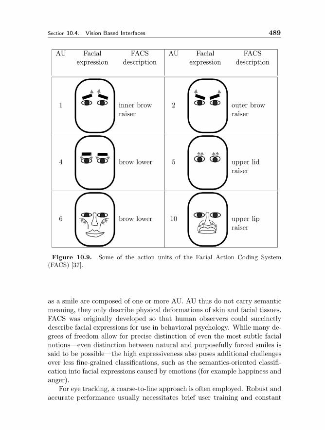
Section 10.4. Vision Based Interfaces 489
AU Facialexpression
FACSdescription
AU Facialexpression
FACSdescription
1 inner browraiser
2 outer browraiser
4 brow lower 5 upper lidraiser
6 brow lower 10 upper lipraiser
Figure 10.9. Some of the action units of the Facial Action Coding System(FACS) [37].
as a smile are composed of one or more AU. AU thus do not carry semanticmeaning, they only describe physical deformations of skin and facial tissues.FACS was originally developed so that human observers could succinctlydescribe facial expressions for use in behavioral psychology. While many de-grees of freedom allow for precise distinction of even the most subtle facialnotions—even distinction between natural and purposefully forced smiles issaid to be possible—the high expressiveness also poses additional challengesover less fine-grained classifications, such as the semantics-oriented classifi-cation into facial expressions caused by emotions (for example happiness andanger).
For eye tracking, a coarse-to-fine approach is often employed. Robust andaccurate performance usually necessitates brief user training and constant
490 Perceptual Interfaces Chapter 10
lighting conditions. Under these conditions, the eye gaze direction can beaccurately estimated despite moderate head translations and rotations.
According to a survey by Donato et al. [31], most approaches to auto-matic analysis of facial expression are either based on optical flow, globalappearance, or local features. The authors re-implemented some of the mostpromising methods and compared their performance on one data set. Op-tical flow methods (such as [85]) were used early on to analyze the shortterm, dynamical evolution of the face. Naturally, these require an image se-quence of the course of a facial expression, and do not apply to static images,due to the lack of motion information. These methods were found to per-form significantly better when the image is not smoothed in a pre-processingstep. This leads to the conclusion that small image artifacts are importantwhen it comes to tracking and/or recognizing facial gestures. Another hintthat high spatial frequencies contribute positively stems from comparing theperformance of Gabor wavelets. Using only high-frequencies had a less detri-mental effect than using only low-frequencies, compared to the baseline ofunrestricted Gabor filters.
Approaches using Gabor filters and Independent Component Analysis(ICA), two methods based on spatially constrained filters, outperformedother methods such as those using PCA or Local Feature Analysis [102]in the investigation by Donato et al. [31]. The authors conclude that lo-cal feature extraction and matching is very important to good performance.This alone is insufficient, however, as the comparison between global and lo-cal PCA-based methods showed. Good performance with less precise featureestimation can be achieved with other methods (e.g., [161].
Global methods that do not attempt to separate the individual contrib-utors to visual appearances seem to be ill-suited to model multi-modal dis-tributions. Refinement of mathematical methods for CV tasks, such as ICA,appears to be promising in order to achieving high accuracy in a variety ofappearance-based applications such as detection, tracking, and recognition.Optical flow and methods that do not attempt to extract FACS action unitsare currently better suited to the real-time demands of VBI.
Handheld Objects
Vision based interfaces that detect and track objects other than human bodyparts—that is, handheld objects used in interaction—have a high potentialfor successful commercial development in the transition period from tradi-tional to perceptual interfaces. Tracking such objects can be achieved morereliably than tracking high DOF body parts, and they may be easier to use
Section 10.4. Vision Based Interfaces 491
than free-form gestures. Handheld artifacts can be used in much the sameway as one’s hands, for example to make pointing gestures, to perform rhyth-mic commands, or to signal the spatial information content of sign languages.Possible useful objects include passive wands [143], objects with active trans-mitters such as LEDs9, and specially colored objects—in fact, anything thatis easily trackable with CV methods. An alternative approach to havingfixed-mounted cameras and tracking moving objects is to embed the camerain the moving object and recognize stationary objects in the environmentor egomotion to enable user interaction. Since detecting arbitrary objects isvery hard, fiducials can make this reverse approach practical [72].
10.4.3 Computer Vision Methods for VBI
In order for a computer vision method to be suitable for VBI, its performancemust meet certain requirements with respect to speed, precision, accuracy,and robustness. A system is said to experience real-time behavior if no delayis apparent between an event (occurrence) and its effect. Precision concernsthe repeatability of observations for identical events. This is particularlyimportant for recognition tasks and biometrics: only if the VBI consistentlydelivers the same result for a given view can this information be used toidentify people or scenes. Accuracy describes the deviation of an observationfrom ground truth. Ground truth must be defined in a suitable format. Thisformat can, for example, be in the image domain, in feature space, or it can bedescribed by models such as a physical model of a human body. It is oftenimpossible to acquire ground truth data, especially if no straightforwardtranslation from observation to the ground truth domain is known. In thatcase, gauging the accuracy of a VBI method may be quite difficult.
Robustness, on the other hand, is easier to determine by exposing theVBI to different environmental conditions, including different lighting (flu-orescent and incandescent lighting and sunlight), different users, clutteredbackgrounds, occlusions (by other objects or self-occlusion), and non-trivialmotion. Generally, the robustness of a vision technique is inversely propor-tional to the amount of information that must be extracted from the scene.
With currently available hardware only a very specific set of fairly fast CVtechniques can be used for truly interactive VBI. One of the most importantsteps is to identify constraints on the problem (regarding the environment orthe user) in order to make simplifying assumptions for the CV algorithms.
9Head trackers can utilize this technology to achieve high accuracy and short la-tencies. One commercial product is the “Precision Position Tracker,” available athttp://www.worldviz.com.
492 Perceptual Interfaces Chapter 10
These constraints can be described by various means. Prior probabilities area simple way to take advantage of likely properties of the object in question,both in image space and in feature space. When these properties vary signif-icantly, but the variance is not random, principal component analysis, neuralnetworks and other learning methods frequently do a good job in extractingthese patterns from training data. Higher-level models can also be employedto limit the search space in the image or feature domain to physically orsemantically possible areas.
Frequently, interface-quality performance can be achieved with multi-modal or multi-cue approaches. For example, combining the results from astereo-based method with those from optical flow may overcome the restric-tions of either method used in isolation. Depending on the desired tradeoffbetween false positives and false negatives, early or late integration (seeFig. 10.3) lends itself to this task. Application- and interface-oriented sys-tems must also address issues such as calibration or adaptation to a particularuser, possibly at runtime, and re-initialization after loss of tracking. Systemstend to become very complex and fragile if many hierarchical stages rely oneach other. Alternatively, flat approaches (those that extract high-level infor-mation straight from the image domain) do not have to deal with schedulingmany components, feedback loops from higher levels to lower levels, andperformance estimation at each of the levels. Robustness in computer visionsystems can be improved by devising systems that do not make irrevoca-ble decisions in the lower layers but instead model uncertainties explicitly.This requires modeling of the relevant processes at all stages, from templatematching to physical object descriptions and dynamics.
All computer vision methods need to specify two things. First, they needto specify the mathematical or algorithmic tool used to achieve the result.This can be PCA, HMM, a neural network, etc. Second, the domain to whichthis tool is applied must be made explicit. Sometimes this will be the rawimage space with gray scale or color pixel information, and sometimes thiswill be a feature space that was extracted from the image by other tools in apre-processing stage. One example would be using wavelets to find particularregions of a face. The feature vector, composed of the image-coordinatelocations of these regions, is embedded in the domain of all possible regionlocations. This can serve as the input to an HMM-based facial expressionanalysis.

Section 10.4. Vision Based Interfaces 493
Edge and Shape Based Methods
Shape properties of objects can be used in three different ways. Fixed shapemodels such as an ellipse for head detection or rectangles for body limbtracking minimize the summative energy function from probe points alongthe shape. At each probe, the energy is lower for sharper edges (in the inten-sity or color image). The shape parameters (size, ellipse foci, rectangular sizeratio) are adjusted with efficient, iterative algorithms until a local minimumis reached. On the other end of the spectrum are edge methods that yield un-constrained shapes. Snakes [67] operate by connecting local edges to globalpaths. From these sets, paths are selected as candidates for recognition thatresemble a desired shape as much as possible. In between these extremes liethe popular statistical shape models, e.g., the Active Shape Model (ASM)[21]. Statistical shape models learn typical deformations from a set of train-ing shapes. This information is used in the recognition phase to registerthe shape to deformable objects. Geometric moments can be computed overentire images or alternatively over select points such as a contour.
These methods require sufficient contrast between the foreground objectand the background, which may be unknown and cluttered. Gradients incolor space [119] can alleviate some of the problems. Even with perfectsegmentation, non-convex objects are not well suited for recognition withshape-based methods since the contour of a concave object can translateinto a landscape with many, deep local minima in which gradient descentmethods get stuck. Only near-perfect initialization allows the iterations todescend into the global minimum.
Color Based Methods
Compelling results have been achieved merely by using skin color properties,e.g., to estimate gaze direction [116] or for interface-quality hand gesturerecognition [71]. This is because the appearance of skin color varies mostly inintensity while the chrominance remains fairly consistent [114]. According toZarit et al. [159], color spaces that separate intensity from chrominance (suchas the HSV color space) are better suited to skin segmentation when simplethreshold-based segmentation approaches are used. However, some of theseresults are based on a few images only, while more recent work examineda huge number of images and found an excellent classification performancewith a histogram-based method in RGB color space as well [61]. It seemsthat simple threshold methods or other linear filters achieve better resultsin HSV space, while more complex methods, particularly learning-based,nonlinear models do well in any color space. Jones et al. [61] also state
494 Perceptual Interfaces Chapter 10
that Gaussian mixture models are inferior to histogram-based approaches,which makes sense given the multi-modality of random image scenes and thefixed amount of Gaussians available to model this. The CAMShift algorithm(Continuously Adaptive Mean Shift) [11, 19] is a fast method to dynamicallyparameterize a thresholding segmentation which is able to deal with a certainamount of lighting and background changes. Together with other imagefeatures such as motion, patches or blobs of uniform color, this makes for afast and easy way to segment skin-colored objects from backgrounds.
Infrared Light: One “color” is particularly well suited to segment humanbody parts from most backgrounds, and that is energy from the infrared (IR)portion of the EM spectrum. All objects constantly emit heat as a functionof their temperature in form of infrared radiation, which are electromagneticwaves in the spectrum from about 700nm (visible red light) to about 1mm(microwaves). The human body emits the strongest signal at about 10µm,which is called long wave IR or thermal infrared. Not many common back-ground objects emit strongly at this frequency in modest climates, thereforeit is easy to segment body parts given a camera that operates in this spec-trum. Unfortunately, this requires very sensitive sensors that often needactive cooling to reduce noise. While the technology is improving rapidly inthis field, the currently easier path is to actively illuminate the body partwith short wave IR. The body reflects it just like visible light, so the il-luminated body part appears much brighter than background scenery to acamera that filters out all other light. This is easily done for short wave IRbecause most digital imaging sensors are sensitive this part of the spectrum.In fact, consumer digital cameras require a filter that limits the sensitivityto the visible spectrum to avoid unwanted effects. Several groups have usedIR in VBI-related projects (e.g., [113, 32, 133]).
Color information can be used on its own for body part localization,or it can create attention areas to direct other methods, or it can serveas a validation and “second opinion” about the results from other methods(multi-cue approach). Statistical color as well as location information is thusoften used in the context of Bayesian probabilities.
Motion Flow and Flow Fields
Motion flow is usually computed by matching a region from one frame toa region of the same size in the following frame. The motion vector forthe region center is defined as the best match in terms of some distancemeasure (e.g., least-squares difference of the intensity values). Note thatthis approach is parameterized by both the size of the region (“feature”) as
Section 10.4. Vision Based Interfaces 495
well as the size of the search neighborhood Other approaches use pyramidsfor faster, hierarchical flow computation; this is especially more efficient forlarge between-frame motions. The most widely used feature tracking methodis the “KLT” tracker. The tracker and the selection of good features to track(usually corners or other areas with high image gradients) are described byShi and Tomasi [120]. KLT trackers have limitations due to the constancyassumption (no change in appearance from frame to frame), match windowsize (aperture problem), and search window size (speed of moving object,computational effort).
A flow field describes the apparent movement of entire scene componentsin the image plane over time. Within these fields, motion blobs are defined aspixel areas of (mostly) uniform motion, i.e., motion with similar speed anddirection. Especially in VBI setups with static camera positions, motionblobs can be very helpful for object detection and tracking. Regions inthe image that are likely locations for a moving body part direct other CVmethods and the VBI in general to these “attention areas.”
The computational effort for tracking image features between frames in-creases dramatically with lower frame rates since the search window size hasto scale according to the tracked object’s estimated maximal velocity. Sincemotion flow computation can be implemented as a local image operation thatdoes not require a complex algorithm or extrinsic state information (only theprevious image patch and a few parameters), it is suited for on-chip com-putation. Comprehensive reviews of optical flow methods can be found inBarron et al. [5] and Mitiche and Bouthemy [89].
Texture and Appearance Based Methods
Information in the image domain plays an important role in every objectrecognition or tracking method. This information is extracted to form im-age features: higher-level descriptions of what was observed. The degreeof abstraction of the features and the scale of what they describe (small,local image artifacts or large, global impressions) have a big impact on themethod’s characteristics. Features built from local image information suchas steep gray-level gradients are more sensitive to noise; they need a goodspatial initialization and frequently a large collection of those features is re-quired. Once these features are found, they need to be brought into contextwith each other, often involving an iterative and computationally expensivemethod with multiple, interdependent and thus more fragile, stages.
If instead the features are composed of many more pixels, cover a largerregion in the image, and abstract to more complex visuals, the methods are
496 Perceptual Interfaces Chapter 10
usually better able to deal with clutter and might flatten the hierarchy ofprocessing levels (since they already contain much more information thansmaller-scale features). The benefits do not come without a price, in thiscase increased computational requirements.
Appearance based methods attempt to identify the patterns that an ob-ject frequently produces in images. The simplest approach to comparing oneappearance to another is to use metrics such as least squared difference ona pixel-by-pixel basis, i.e., the lowest-level feature vector. This is not veryefficient and is too slow for object localization or tracking. The key is toencode as much information as possible in an as small as possible featurevector—to maximize the entropy.
One of the most influential procedures uses a set of training images andthe Karhunen-Loeve transform [65, 81]. This transformation is an orthogo-nal basis rotation of the training space that maximizes sample variance alongthe new basis vectors and is frequently known in the computer vision liter-ature as principal component analysis (PCA) [59] and is directly related tosingular value decomposition (SVD). In the well-known Eigenfaces approach,Turk and Pentland [134] applied this method to perform face detection andrecognition, extending the work by Kirby and Sirovich for image representa-tion and compression [70]. Active Appearance Models (AAMs) [20] encodeshape and appearance information in one model, built in a two-step processwith PCA. Active Blobs [118] are similar to AAM. In these approaches, theobserved object appearance steers object tracking by guiding initializationfor subsequent frames, similar to the concept of the Kalman filter. Duringtraining, a parameterization is learned that correlates observation-estimationerror with translational offsets.
A Gabor wavelet is a sine wave enveloped by a Gaussian, modeled afterthe function of the human visual cortical cell [106, 60, 29, 25]. Wavelets arewell suited to encode both spatial and frequency information in a compact,parameterized representation. This alleviates problems of FFT approacheswhere all local spatial information is lost. Feris et al. [117] showed goodface tracking performance with a hierarchical wavelet network, a collectionof collections of wavelets. Each feature is represented by a set of wavelets,enabling tracking in the manner of KLT trackers, but comparatively morerobust to lighting and deformation changes.
Another approach to learn and then test for common appearances ofobjects is to use neural networks; however, in some cases their performance(in terms of speed and accuracy) has been surpassed by other methods.One extremely fast detection procedure proposed by Viola and Jones [139]has attracted much attention. In this work, very simple features based on
Section 10.4. Vision Based Interfaces 497
intensity comparisons between rectangular image areas are combined by Ada-boosting into a number of strong classifiers. These classifiers are arranged insequence and achieve excellent detection rates on face images with a low falsepositive rate. The primary advantage of their method lies in the constant-time computation of features that have true spatial extent, as opposed toother techniques that require time proportional to the area of the extent.This allows for very high speed detection of complex patterns at differentscales. However, the method is rotation-dependent.
A more complete review of appearance-based methods for detection andrecognition of patterns (faces) can be found in Yang et al.’s survey on facedetection [155].
Background Modeling
Background modeling is often used in VBI to account for (or subtract away)the non-essential elements of a scene. There are essentially two techniques:segmentation by thresholding and dynamic background modeling.
Thresholding requires that the foreground object has some unique prop-erty that distinguishes it from all or most background pixels. For example,this property can be foreground brightness, so that a pixels with values abovea particular gray scale intensity threshold are classified as foreground, andvalues below as belonging to the background. Color restrictions on the back-ground are also an effective means for simple object segmentation. There, itis assumed that the foreground object’s color does not appear very frequentlyor in large blobs in the background scene. Of course, artificial coloring ofthe foreground object avoids problems induced by wildly varying or unknownobject colors—e.g., using a colored glove for hand detection and tracking.
Dynamic Background Modeling requires a static camera position. Thevalues of each pixel are modeled over time with the expectation to find apattern of values that this pixel assumes. The values may be described bya single contiguous range, or it may be multi-modal (two or more contigu-ous ranges). If the value suddenly escapes these boundaries that the modeldescribes as typical, the pixel is considered part of a foreground object thattemporarily occludes the background. Foreground objects that are station-ary for a long time will usually be integrated into the background modelover time and segmentation will be lost. The mathematics to describe thebackground often use statistical models with one or more Gaussians [48].
498 Perceptual Interfaces Chapter 10
Temporal Filtering and Modeling
Temporal filtering typically involves methods that go beyond motion flow totrack on the object or feature level, rather than at the pixel or pattern level.For example, hand and arm gesture recognition (see subsection Hand andArm Gestures in 4D on page 485) requires temporal filtering.
Once the visual information has been extracted and a feature vector hasbeen built, general physics-based motion models are often used. For example,Kalman filtering in combination with a skeletal model can deal with resolvingsimple occlusion ambiguities [146]. Other readily available mathematicaltools can be applied to the extracted feature vectors, independently of thepreceding CV computation. Kalman filtering takes advantage of smoothmovements of the object of interest. At every frame, the filter predicts theobject’s location based on the previous motion history. The image matchingis initialized with this prediction, and once the object is found, the Kalmanparameters are adjusted according to the prediction error.
One of the limitations of Kalman filtering is the underlying assumptionof a Gaussian probability. If this is not the case, and the probability func-tion is essentially multi-modal as it is the case for scenes with clutteredbackgrounds, Kalman filtering cannot cope with the non-Gaussian obser-vations. The particle filtering or factored sampling method, often calledCondensation (conditional density propagation) tracking, has no implicit as-sumption of a particular probability function but rather represents it witha set of sample points of the function. Thus, irregular functions with mul-tiple “peaks”—corresponding to multiple hypotheses for object states—canbe handled without violating the method’s assumptions. Factored samplingmethods [55] have been applied with great success to tracking of fast-moving,fixed-shape objects in very complex scenes [76, 28, 14]. Various models, onefor each typical motion pattern, can improve tracking, as shown by Isardand Blake [56]. Partitioned sampling reduces the computational complexityof particle filters [82]. The modeled domain is usually a feature vector, com-bined from shape-describing elements (such as the coefficients of B-splines)and temporal elements (such as the object velocities).
Dynamic gesture recognition, i.e., recognition and semantic interpreta-tion of continuous gestures and body motions, is an essential part of percep-tual interfaces. Temporal filters exploit motion information only to improvetracking, while the following methods aim at detecting meaningful actionssuch as waving a hand for goodbye.
Discrete approaches can perform well at detecting spatio-temporal pat-terns [51]. Most methods in use, however, are borrowed from the more
Section 10.4. Vision Based Interfaces 499
evolved field of speech recognition due to the similarity of the domains: multi-dimensional, temporal, and noisy data. Hidden Markov Models (HMMs)[15, 158] are frequently employed to dissect and recognize gestures due totheir suitability to processing temporal data. However, the learning meth-ods of traditional HMMs cannot model some structural properties of movinglimbs very well.10 Brand [13] uses another learning procedure to train HMMsthat overcomes these problems. This allows for estimation of 3D model con-figurations from a series of 2D silhouettes and achieves excellent results. Theadvantage of this approach is that no knowledge has to be hard-coded butinstead everything is learned from training data. This has its drawbackswhen it comes to recognizing previously unseen motion.
Higher-level Models
To model a human body or its parts very precisely such as is required forcomputer graphics applications, at least two models are necessary. One com-ponent describes the kinematic structure of the skeleton, the bone connec-tions and the joint characteristics. Even complex objects such as the entirehuman body or the hand can thus—with reasonable accuracy—be thoughtof as a kinematic chain of rigid objects. The second component describesthe properties of the flesh around the bones, either as a surface model or asa volumetric model. Very complex models that even describe the behaviorof skin are commonplace in the animation industry. Additional models arefrequently used to achieve even greater rendering accuracy, such as modelsof cloth or hair.
Computer vision can benefit from these models to a certain degree. Astructural, anatomical 3D model of the human body has advantages over a2D model because it has explicit knowledge of the limbs and the fact thatthey can occlude each other from a particular view [110]. Given a kinematicmodel of the human body (e.g., [77]), the task to estimate the limb locationsbecomes easier compared to the case when the knowledge of interdependencyconstraints is lacking. Since the locations and orientations of the individualrigid objects (limbs, phalanges) are constrained by their neighboring chainlinks, the effort to find them in the image decreases dramatically.
It is important for VBI applications to exploit known characteristics ofthe object of interest as much as possible. A kinematic model does exactlythat, as do statistical models that capture the variation in appearance from
10Brand [13] states that the traditional learning methods are not well suited to modelstate transitions since they do not improve much on the initial guess about connectivity.Estimating the structure of a manifold with these methods thus is extremely suboptimalin its results.
500 Perceptual Interfaces Chapter 10
a given view point or the variation of shape (2D) or form (3D). Often themodel itself is ad hoc, that is, it is manually crafted by a human based onprior knowledge of the object. The model’s parameter range is frequentlylearned from training data.
Higher-level models describe properties of the tracked objects that arenot immediately visible in the image domain. Therefore a translation be-tween image features and model parameters needs to occur. A frequentlyused technique is analysis by synthesis in which the model parameters areestimated by an iterative process. An initial configuration of the model isback-projected into the image domain. The difference between projectionand observation then drives adjustment of the parameters, following anotherback-projection into the image domain and so forth until the error is suf-ficiently small (e.g., see Kameda et al. [64] and Strom et al. [130]). Thesemethods lack the capability to deal with singularities that arise from am-biguous views [92]. When using more complex models that allow methodsfrom projective geometry to be used to generate the synthesis, self-occlusionis modeled again and thus it can be dealt with. Stenger et al. [128]. usea recently proposed modification of the Kalman filter, the so-called an “un-scented Kalman filter” [62] to align the model with the observations. Despitespeed and accuracy advantages over more traditional approaches, the maindrawbacks of all Kalman-based filters however is that they assume a uni-modal distribution. This assumption is most likely violated by complex,articulated objects such as the human body or the hand.
Particle filtering methods for model adjustment are probably better suitedfor more general applications because they allow for any kind of underlyingdistribution, even multi-modal distributions. Currently, their runtime re-quirements are not immediately suitable for real-time operation yet, butmore efficient modifications of the original algorithm are available.
Real-time Systems, Frame Rate, Latency, Processing Pipelines
Most user interfaces require real-time responses from the computer: for feed-back to the user, to execute commands immediately or both. But whatexactly does real-time mean for a computer vision application?
There is no universal definition for real-time in computer terms. However,a system that responds to user input is said to operate in real-time if theuser of the system perceives no delay between action command and action.Hence, real-time pertains to a system’s ability to respond to an event withoutnoticeable delay. The opposite would be a delayed response, a response aftera noticeable processing time. Mouse input, for example, is usually processed
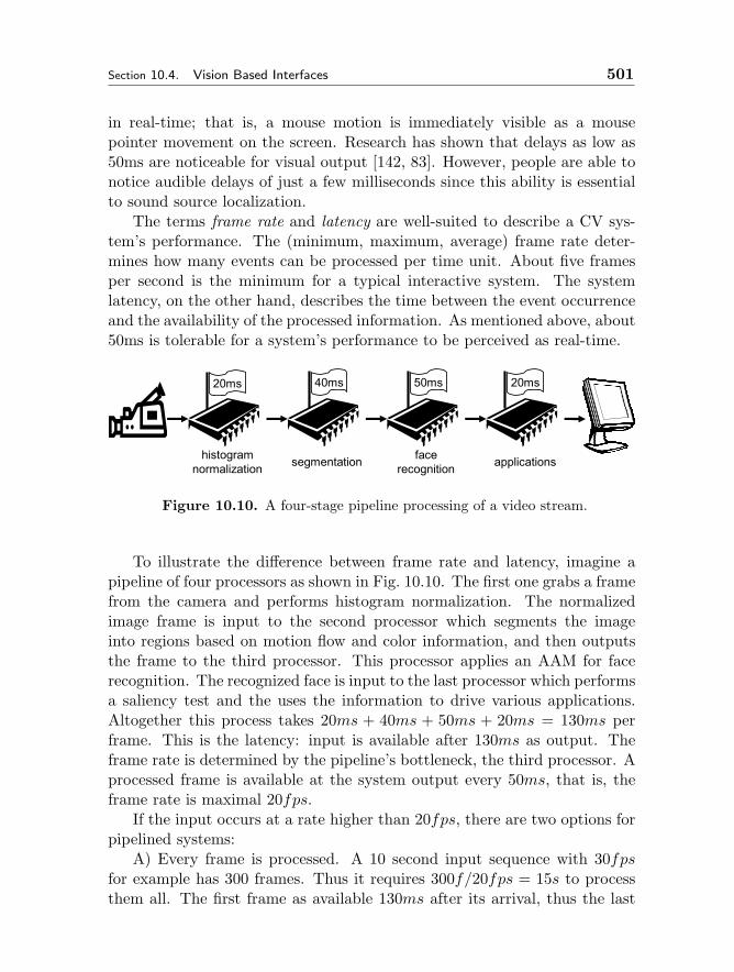
Section 10.4. Vision Based Interfaces 501
in real-time; that is, a mouse motion is immediately visible as a mousepointer movement on the screen. Research has shown that delays as low as50ms are noticeable for visual output [142, 83]. However, people are able tonotice audible delays of just a few milliseconds since this ability is essentialto sound source localization.
The terms frame rate and latency are well-suited to describe a CV sys-tem’s performance. The (minimum, maximum, average) frame rate deter-mines how many events can be processed per time unit. About five framesper second is the minimum for a typical interactive system. The systemlatency, on the other hand, describes the time between the event occurrenceand the availability of the processed information. As mentioned above, about50ms is tolerable for a system’s performance to be perceived as real-time.
20ms 40ms 50ms 20ms
histogramnormalization
segmentationface
recognitionapplications
Figure 10.10. A four-stage pipeline processing of a video stream.
To illustrate the difference between frame rate and latency, imagine apipeline of four processors as shown in Fig. 10.10. The first one grabs a framefrom the camera and performs histogram normalization. The normalizedimage frame is input to the second processor which segments the imageinto regions based on motion flow and color information, and then outputsthe frame to the third processor. This processor applies an AAM for facerecognition. The recognized face is input to the last processor which performsa saliency test and the uses the information to drive various applications.Altogether this process takes 20ms + 40ms + 50ms + 20ms = 130ms perframe. This is the latency: input is available after 130ms as output. Theframe rate is determined by the pipeline’s bottleneck, the third processor. Aprocessed frame is available at the system output every 50ms, that is, theframe rate is maximal 20fps.
If the input occurs at a rate higher than 20fps, there are two options forpipelined systems:
A) Every frame is processed. A 10 second input sequence with 30fpsfor example has 300 frames. Thus it requires 300f/20fps = 15s to processthem all. The first frame as available 130ms after its arrival, thus the last
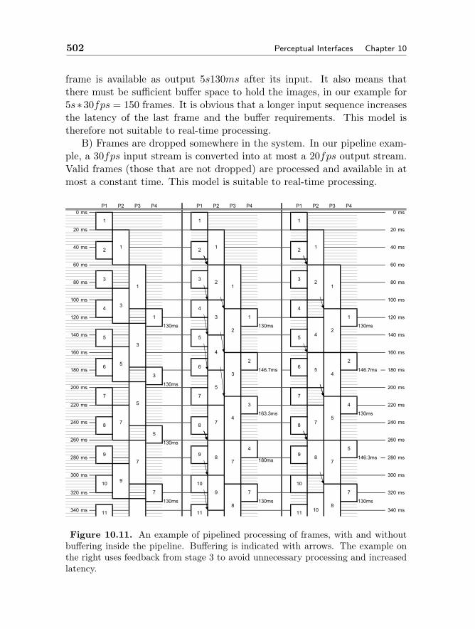
502 Perceptual Interfaces Chapter 10
frame is available as output 5s130ms after its input. It also means thatthere must be sufficient buffer space to hold the images, in our example for5s∗30fps = 150 frames. It is obvious that a longer input sequence increasesthe latency of the last frame and the buffer requirements. This model istherefore not suitable to real-time processing.
B) Frames are dropped somewhere in the system. In our pipeline exam-ple, a 30fps input stream is converted into at most a 20fps output stream.Valid frames (those that are not dropped) are processed and available in atmost a constant time. This model is suitable to real-time processing.
P1 P2 P3 P4 P1 P2 P3 P4 P1 P2 P3 P4
ms
ms
ms
ms
ms
ms
ms
ms
ms
ms
ms
ms
ms
ms
ms
ms
ms
ms
ms
ms
ms
ms
ms
ms
ms
ms
ms
ms
ms
60
40
0
20
140
120
100
80
220
200
180
160
300
280
260
240
340
320 ms
ms
130ms
10
130ms
146.7ms
130ms
146.3ms
2
4
4
4
7
130ms
130ms
130ms
130ms
5
11
7
9
7
59
7
7
10
8
8
11
1
5
6
7
5
5
78
1
3
4
2
2
1
12
3
5
6
7
8
9
10
340
260
280
300
320
140
160
180
200
1
1
220
240
3
3
5
5
100
4
1
120
3
40
60
80
ms
ms
ms
ms
1
0
20
2
ms
5
1
2
3
4
5
7
8
7
8
6
1
2
3
4
9
9
10
11
3
2
146.7ms
1
1
130ms2
4
7
8
7
130ms
4
3
163.3ms
180ms
Figure 10.11. An example of pipelined processing of frames, with and withoutbuffering inside the pipeline. Buffering is indicated with arrows. The example onthe right uses feedback from stage 3 to avoid unnecessary processing and increasedlatency.
Section 10.4. Vision Based Interfaces 503
Dropping frames, however, brings about other problems. There are twocases: First, there is no buffer available anywhere in the system, not evenfor partial frames. This is shown on the left hand side in Fig. 10.11. Inour example, the first processor has no problems keeping up with the inputpace, but the second processor will still be working on the first frame when itreceives the second frame 33.3ms after arrival of the first. The second frameneeds to be dropped. Then the second processor would idle for 2 ∗ 33.3ms−40ms = 26.7ms. Similar examples can be constructed for the subsequentpipeline stages.
Second, frames can be buffered at each pipeline stage output or input.This is shown in the center drawing of Fig. 10.11. It assumes no extracommunication between the pipeline stages. Each subsequent stage requestsa frame as soon as it completed processing one frame, and the precedingstage keeps the latest processed frame around in a buffer until it can replaceit with the next processed frame. In the example, the second frame would bebuffered for 6.7ms at the transition to the second processor, the third framefor 2∗40ms−2∗33.3ms = 13.3ms, the fourth for 3∗40ms−3∗33.3ms = 20ms,etc. The highest latency after the 2nd stage would be for every fifth frame,which is buffered for a total of 5 ∗ 40ms − 5 ∗ 33.3ms = 33.3ms beforeprocessing. Then in fact the next processed frame (frame number 7) isfinished being processed already and is sent to stage 3 instead of the bufferedframe, which is dropped. These latencies can accumulate throughout thepipeline. The frame rate is maximal (20fps) in this example, but some ofthe frames’ latencies have increased dramatically.
The most efficient method in terms of system latency and buffer usagefacilitates pipeline feedback from the later stages to the system input, asshown on the right in Fig. 10.11. The feedback is used to adjust everystages’ behavior in order to maximize utilization of the most time criticalstage in the pipeline. Alternatively to the scenario shown, it is also possibleto buffer frames only buffered before the first stage, and feed them into thesystem with a speed that the pipeline’s bottleneck stage can keep up with.This is not shown, but it completely avoids the need for in-pipeline buffering.Note that even in this efficient scenario with pipeline feedback the increasedframe rates in comparison to the leftmost case are bought with an increasein average latency.
Examples of architectures that implement component communicationand performance optimizing scheduling are the “Quality-Control Manage-ment” in the DirectShow subsystem of Microsoft’s DirectX technology andthe “Modular Flow Scheduling Middleware” [40].
504 Perceptual Interfaces Chapter 10
10.4.4 VBI Summary
Vision-Based Interfaces have numerous applications; the potential of VBIhas only begun to be explored. But computational power is getting to astage where it can handle the vast amounts of data of live video streams.Progress has been made in many relevant areas of computer vision; manymethods have been demonstrated that begin to provide human-computer in-terface quality translation of body actions into computer commands. Whilea large amount of work is still required to improve the robustness of thesemethods, especially in modeling and tracking highly articulated objects, thecommunity has begun to take steps towards standardizing interfaces of popu-lar methods and providing toolkits for increasingly higher level tasks. Theseare important steps in bringing the benefits of VBI to a wider audience.
The number of consumer-grade commercial applications of computer vi-sion has significantly increased in recent years, and this trend will continuedriven by ongoing hardware progress. To advance the state of the art ofVBI—at the intersection of the disciplines of CV and HCI—it is vital to es-tablish evaluation criteria, such as benchmarks for the quality and speed ofthe underlying methods and the resulting interfaces. Evaluation databasesmust be made accessible for all components of VBI (such as those alreadyavailable for faces), both for static images and increasingly dynamic data forreal-time video processing.
10.5 Brain-Computer Interfaces
Perhaps the ultimate interface to computers would be a direct link to thethoughts and intentions of the user, a “Your wish is my command” modelof interaction, involving no physical action or interpretation of any kind.While this kind of mind-reading technology is not likely to be developed inthe foreseeable future, the nascent research area of Brain-Computer Inter-faces (BCI) is perhaps a step in this direction. BCI technology attempts toperceive commands or control parameters by sensing relevant brain activityof the user. While not fitting completely within the perceptual interfacemodel of natural human-human interaction, BCI may eventually be an inte-gral component of perceptual interfaces. The computer vision community’sextensive experience with learning, statistical, and other pattern recognitionmethods and techniques can be of tremendous value to this new field.
A Brain-Computer Interface does not depend on the brain’s normal out-put channels of peripheral nerves and muscles, but instead measures elec-trical activity either at the scalp or in the cortex. By measuring the elec-

Section 10.5. Brain-Computer Interfaces 505
troencephalographic (EEG) activity at the scalp, certain features of the EEGsignal can be used to produce a control signal. Alternatively, implanted elec-trodes can be used to measure the activity of individual cortical neurons oran array of neurons. These technologies have primarily been targeted tobe used by people with neuromuscular impairments that prevent them fromcommunicating via conventional methods. In recent years, researchers havebegun to consider more general uses of the technologies. A review by Wolpawet al. [144] notes that while the rising interest in BCI technologies in recentyears has produced exciting developments with considerable promise, theyare currently low-bandwidth devices with a maximum information transferrate of 10 to 25 bits per minute, and this rate is likely to improve onlygradually.
Wolpaw et al. argue that, in order to make progress in brain-computerinterfaces, researchers must understand that BCI is not simply mind readingor “wire-tapping” the brain, determining a person’s thoughts and intentionsby listening in on brain activity. Rather, BCI should be considered as a newoutput channel for the brain, one that is likely to require training and skillto master.
“Brain-Machine Interface” [97] is the traditional term as it grew out ofinitial uses of the technology: to interface to prosthetic devices. Sensors wereimplanted primarily in motoric nerves in the extremities and a one-to-onefunction was typically used to map the sensor outputs to actuator controlsignals. “Brain-Computer Interface” more accurately captures the neces-sity for computational power between the neuro-sensors and the controlleddevices or application-specific software. As the sensors increasingly moveinto the brain (intracortical electrodes) and target not only motoric nervesbut generic neurons, the mapping from neuron activity to (desired, normal,or pathologic) output becomes less direct. Complex mathematical modelstranslate the activity of many neurons into a few commands—computationalneuroscience focuses on such models and their parameterizations. Mathe-matical models that have proven to be well suited to the task of replicatinghuman capabilities, in particular the visual sense, seem to perform well forBCIs as well—for example, particle and Kalman filters [149]. Two featureextraction and classification methods frequently used for BCIs are reviewedin Ebrahimi et al. [35].
Figure 10.12 schematically explains the principles of a BCI for prostheticcontrol. The independent variables, signals from one or many neural sensors,are processed with a mathematical method and translated into the depen-dent variables, spatial data that drives the actuators of a prosthetic device.Wolpaw et al. [144] stress that BCI should eventually comprise three levels
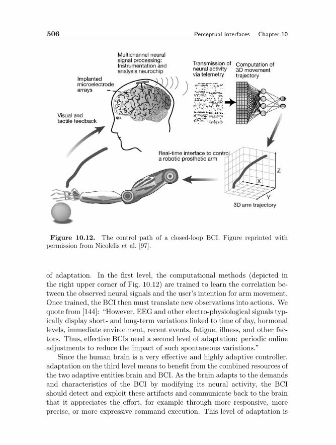
506 Perceptual Interfaces Chapter 10
Figure 10.12. The control path of a closed-loop BCI. Figure reprinted withpermission from Nicolelis et al. [97].
of adaptation. In the first level, the computational methods (depicted inthe right upper corner of Fig. 10.12) are trained to learn the correlation be-tween the observed neural signals and the user’s intention for arm movement.Once trained, the BCI then must translate new observations into actions. Wequote from [144]: “However, EEG and other electro-physiological signals typ-ically display short- and long-term variations linked to time of day, hormonallevels, immediate environment, recent events, fatigue, illness, and other fac-tors. Thus, effective BCIs need a second level of adaptation: periodic onlineadjustments to reduce the impact of such spontaneous variations.”
Since the human brain is a very effective and highly adaptive controller,adaptation on the third level means to benefit from the combined resources ofthe two adaptive entities brain and BCI. As the brain adapts to the demandsand characteristics of the BCI by modifying its neural activity, the BCIshould detect and exploit these artifacts and communicate back to the brainthat it appreciates the effort, for example through more responsive, moreprecise, or more expressive command execution. This level of adaptation is
Section 10.6. Summary 507
difficult to achieve, but promises to yield vastly improved performance.The number of monitored neurons necessary to accurately predict a task
such as 3D arm movement is open to debate. Early reports employed open-loop (no visual feedback to the study subject) experiments with offline modelbuilding and parameterization. Those studies suggest by extrapolation thatbetween 400 and 1350 neurons are necessary, depending on the brain area inwhich the sensors are implanted [141]. A more recent study by Taylor et al.provided real-time visual feedback and repeatedly updated the mathemati-cal model underlying the translation function from neurons to the controlledobject [132, 97]. They used only 18 neurons to achieve sufficient performancefor a 2D cursor task, with the closed-loop method being significantly supe-rior to the open-loop method. Currently, up to about 100 neurons can berecorded simultaneously. All currently used electro-physiological artifactscan be detected with a temporal resolution of 10ms to 100ms, but somedevelop only over the course of many seconds.
In addition to the “input” aspect of BCIs, there are several examplesof the reverse technology: computers connecting into the sensorimotor sys-tem providing motor output to the human (see [22]). Well-known examplesinclude heart pace makers and cochlear implants, which directly stimulateauditory nerves, obviating the need for a mechanical hearing mechanism.Another device is able to prevent tremors caused by Parkinson’s disease or“Essential Tremor” by blocking erroneous nervous signals from reaching thethalamus where they would trigger involuntary muscle contractions [88].
10.6 Summary
The topic of perceptual interfaces is very broad, covering many technolo-gies and their applications in advanced human-computer interaction. Inthis chapter we have attempted to give an overview of perceptual interfacesand go a bit deeper into how the field of computer vision can contribute tothe larger goal of natural, adaptive, multimodal, interactive interfaces. Vi-sion based interaction (VBI) is useful in itself, providing information abouthuman identity, location, movement, and expression through non-invasiveand non-intrusive methods. VBI has many near-term application areas, in-cluding computer games, accessibility, intelligent environments, biometrics,movement analysis, and social robots.
If the technical goal of building perceptual interfaces can be achieved toany reasonable degree, the ways in which people interact with computers—and with technology in general—will be transformed significantly. In addi-tion to computer vision, this will require advances in many areas, includ-
508 Perceptual Interfaces Chapter 10
ing speech and sound recognition and synthesis, natural language process-ing, user modeling, haptic and tangible interfaces, and dialogue modeling.More difficult yet, it will require collaboration and integration among thesevarious research areas. In recent years, several workshops and conferenceshave begun to focus on these issues, including the Workshop on Percep-tual/Perceptive User Interfaces (PUI), the International Conference on Mul-timodal Interfaces (ICMI), and International Conference on Intelligent UserInterfaces (IUI). In addition, large major conference that atract a wide vari-ety of participants—such as CHI and SIGGRAPH—now frequently showcaseperceptual interface research or demonstrations.
As the separate technical communities continue to interact and worktogether on these common goals, there will be a great need for multimodaldata sets for training and testing perceptual interfaces, with task data, video,sound, etc., and associated ground truth. Building such a database is notan easy task. The communities will also need standard benchmark suites forobjective performance evaluation, similar to those that exist for individualmodalities of speech, fingerprint, and face recognition. Students need tobe trained to be conversant with multiple disciplines, and courses must bedeveloped to cover various aspects of perceptual interfaces.
The fact that perceptual interfaces have great promise but will requireherculean efforts to reach technical maturity leads to the question of short-and medium-term viability. One possible way to move incrementally towardthe long-term goal is to to “piggyback” on the current paradigm of graph-ical user interfaces. Such a “strawman perceptual interface” could start byadding just a few new events in the standard event stream that is part oftypical GUI-based architectures. The event stream receives and dispatchesevents of various kinds: mouse movement, mouse button click and release,keyboard key press and release, window resize, etc. A new type of event—a“perceptual event”—could be added to this infrastructure that would, forexample, be generated when a person enters the visual scene in front of thecomputer; or when a person begins to speak; or when the machine (or objectof interest) is touched; or when some other simple perceptual event takesplace. The benefit of adding to the existing GUI event-based architectureis that thousands upon thousands of developers already know how to dealwith this architecture and how to write event handlers that implement vari-ous functionality. Adding even a small number of perceptual events to thisstructure would allow developers to come up with creative novel uses forthem, and help lead to their acceptance in the marketplace.
This proposed development framework leads raises several questions.Which percepual events would be most useful and feasible to implement?
Bibliography 509
Is the event-based model the best way to bootstrap perceptual interfaces?Can we create perceptual events that are reliable enough to be useful? Howshould developers think about non-deterministic events (as opposed to cur-rent events, which are for all practical purposes deterministic)? For example,will visual events work when the lights are turned off, or if the camera lensis obstructed?
There are numerous issues, both conceptual and practical, surroundingthe idea of perceptual interfaces. Privacy is one of the utmost importance.What are the implications of having microphones, cameras, and other sensorsin computing environments? Where does the data go? What behavioralparameters are stored or sent elsewhere? To have any chance of success,these issues must be dealt with directly, and it must be made clear to usersexactly where the data goes (and does not go). Acceptance of perceptualinterfaces depends on instilling confidence that one’s privacy is not violatedin any way.
Some argue against the idea of interface technologies that attempt tobe intelligent or anthropomorphic, claiming that HCI should be character-ized by direct manipulation, providing the user with predictable interac-tions that are accompanied by a sense of responsiblity and accomplishment[121, 122, 123, 126, 125]. While these arguments seem quite appropriatefor some uses of computers—particularly when a computer is used as a toolfor calculations, word processing, and the like—it appears that future com-puting environments and uses will be well suited for adaptive, intelligent,agent-based perceptual interfaces.
Another objection to perceptual interfaces is that they just won’t work,that the problems are too difficult to be solved well enough to be useful. Thisis a serious objection—the problems are, indeed, very difficult. It would notbe so interesting otherwise. In general, we subscribe to the “If you buildit, they will come” school of thought. Building it is a huge and excitingendeavor, a grand challenge for a generation of researchers in multiple disci-plines.
Bibliography
[1] E. Andr and T. Rist. Presenting through performing: on the use of multiplelifelike characters in knowledge-based presentation systems. In Proceedings ofthe 5th international conference on Intelligent user interfaces, pages 1–8. ACMPress, 2000.
[2] R. Azuma, J. W. Lee, B. Jiang, J. Park, S. You, and U. Neumann. Tracking inUnprepared Environments for Augmented Reality Systems. ACM Computers& Graphics, 23(6):787–793, December 1999.
510 Perceptual Interfaces Chapter 10
[3] G. Ball and J. Breese. Emotion and Personality in a Conversational Character.In Workshop on Embodied Conversational Characters, pages 83–84, October1998.
[4] G. Ball, D. Ling, D. Kurlander, J. Miller, D. Pugh, T. Skelly, A. Stankosky,D. Thiel, M. van Dantzich, and T. Wax. Lifelike computer characters: the per-sona project at Microsoft. In J. Bradshaw, editor, Software Agents. AAAI/MITPress, 1997.
[5] J. L. Barron, D. J. Fleet, and S. S. Beauchemin. Performance of Optical FlowTechniques. Int. Journal of Computer Vision, 12(1):43–77, 1994.
[6] J. N. Bassili. Emotion recognition: The role of facial movement and the relativeimportance of upper and lower areas of the face. Journal of Personality andSocial Psychology, 37:2049–2059, 1979.
[7] J. Biggs and M. A. Srinivasan. Haptic interfaces. In K. Stanney, editor, Hand-book of Virtual Environments. Lawrence Earlbaum, Inc., 2002.
[8] S. Birchfield. Elliptical head tracking using intensity gradients and color his-tograms. In Proceedings of the IEEE Conference on Computer Vision andPattern Recognition, pages 232–237, June 1998.
[9] M. J. Black and Y. Yacoob. Recognizing Facial Expressions in Image Sequences,Using Local Parameterized Models of Image Motion. Int. Journal of ComputerVision, 25(1):23–48, 1997.
[10] R. A. Bolt. Put-That-There: Voice and Gesture in the Graphics Interface.Computer Graphics, ACM SIGGRAPH, 14(3):262–270, 1980.
[11] G.R. Bradski. Real-time face and object tracking as a component of a percep-tual user interface. In IEEE Workshop on Applications of Computer Vision,pages 142–149, 1998.
[12] A. Braffort, C. Collet, and D. Teil. Anthropomorphic model for hand ges-ture interface. In Proceedings of the CHI ’94 conference companion on Humanfactors in computing systems, April 1994.
[13] M. Brand. Shadow Puppetry. In ICCV, 1999.[14] L. Bretzner, I. Laptev, and T. Lindeberg. Hand gesture recognition using multi-
scale colour features, hierarchical models and particle filtering, 2002.[15] H. Bunke and T. Caelli, editors. Hidden Markov Models in Vision, volume
15(1) of International Journal of Pattern Recognition and Artificial Intelligence.World Scientific Publishing Company, 2001.
[16] J. Cassell. Embodied conversational interface agents. Communications of theACM, 43(4):70–78, 2000.
[17] T. Choudhury, B. Clarkson, T. Jebara, and A. Pentland. Multimodal PersonRecognition using Unconstrained Audio and Video. In Proceedings of the SecondConference on Audio- and Video-based Biometric Person Authentication, 1999.
[18] P. R. Cohen, M. Johnston, D. McGee, S. Oviatt, J. Pittman, I. Smith, L. Chen,and J. Clow. Quickset: Multimodal interaction for distributed applications. InProceedings of the Fifth International Multimedia Conference (Multimedia ’97),pages 31–40. ACM Press, 1997.
[19] D. Comaniciu, V. Ramesh, and P. Meer. Real-Time Tracking of Non-RigidObjects Using Mean Shift. In IEEE CVPR, volume 2, pages 142–149, 2000.
Bibliography 511
[20] T. F. Cootes, G. J. Edwards, and C. J. Taylor. Active Appearance Models. InProc. European Conference on Computer Vision, pages 484–498, 1998.
[21] T.F. Cootes and C.J. Taylor. Active Shape Models: Smart Snakes. In Proceed-ings of the British Machine Vision Conference, pages 9–18. Springer-Verlag,1992.
[22] W. Craelius. Bionic Man: Restoring Mobility. Science, 295(5557):1018–1021,February 2002.
[23] R. Cutler and M. Turk. View-based Interpretation of Real-time Optical Flowfor Gesture Recognition. In Proceedings of the Third IEEE Conference on Faceand Gesture Recognition, Nara, Japan, pages 416–421, April 1998.
[24] T. Darrell, G. Gordon, M. Harville, and J. Woodfill. Integrated Person TrackingUsing Stereo, Color, and Pattern Detection. In Proc. IEEE Conference onComputer Vision and Pattern Recognition (CVPR), pages 601–609, June 1998.
[25] J. G. Daugman. Complete Discrete 2D Gabor Transform by Neural Networksfor Image Analysis and Compression. IEEE Trans. Acoustics, Speech, andSignal Processing, 36:1169–1179, 1988.
[26] J. Davis and M. Shah. Visual Gesture Recognition. In Vision, Image, andSignal Processing, volume 141, pages 101–106, April 1994.
[27] D. DeCarlo and D.N. Metaxas. Optical Flow Constraints on Deformable Modelswith Applications to Face Tracking. Int. Journal of Computer Vision, 38(2):99–127, 2000.
[28] J. Deutscher, A. Blake, and I. Reid. Articulated Body Motion Capture by An-nealed Particle Filtering. In Proc. IEEE Conf on CV and Pattern Recognition,volume 2, pages 126–133, 2000.
[29] R. DeValois and K. DeValois. Spatial Vision. Oxford Press, 1988.[30] A. Dix, J. Finlay, G. Abowd, and R. Beale. Human-Computer Interaction,
Second Edition. Prentice Hall Europe, 1998.[31] G.a Donato, M.S. Bartlett, J.C. Hager, P. Ekman, and T.J. Sejnowski. Clas-
sifying Facial Actions. IEEE Transactions on Pattern Analysis and MachineIntelligence, 21(10):974–989, October 1999.
[32] K. Dorfmuller-Ulhaas and D. Schmalstieg. Finger Tracking for Interaction inAugmented Environments. In IFAR, 2001.
[33] F. Dornaika and J. Ahlberg. Face Model Adaptation using Robust Matchingand the Active Appearance Algorithm. In IEEE Workshop on Applications ofComputer Vision (WACV), pages 3–7, December 2002.
[34] A. Doucet, N. de Freitas, and N. J. Gordon, editors. Sequential Monte CarloMethods in Practice. Springer-Verlag, 2001.
[35] T. Ebrahimi, J.-M. Vesin, and G. Garcia. Brain-Computer Interface in Multi-media Communication. IEEE Signal Processing Magazine, January 2003.
[36] D. Efron. Gesture, Race and Culture. King’s Crown Press, New York, 1941.[37] P. Ekman and W.V. Friesen. The facial action coding system: A technique for
the measurement of facial movement. Consulting Psychologists Press, 1978.[38] R. Feris, V. Krueger, and R. Cesar Jr. Efficient Real-Time Face Tracking
in Wavelet Subspace. In ICCV’01 Workshop on Recognition, Analysis andTracking of Faces and Gestures in Real-Time Systems, Vancouver, BC, Canada,2001.

512 Perceptual Interfaces Chapter 10
[39] P. M. Fitts. The information capacity of the human motor system in controllingthe amplitude of movement. Journal of Experimental Psychology, 47:381–391,1954.
[40] A.R.J. Franois and G.G. Medioni. A Modular Software Architecture for Real-Time Video Processing. In Proceedings of the International Workshop on Com-puter Vision Systems, July 2001.
[41] W. T. Freeman and M. Roth. Orientation histograms for hand gesture recog-nition. In Proceedings of the International Workshop on Automatic Face andGesture Recognition, pages 296–301. IEEE Computer Society, June 1995.
[42] M. Fukumoto, Y. Suenaga, and K. Mase. Finger-Pointer: Pointing Interface byImage Processing. Computers & Graphics, 18(5):633–642, 1994.
[43] D.M. Gavrila. The Visual Analysis of Human Movement: A Survey. ComputerVision and Image Understanding, 73(1):82–98, 1999.
[44] J. Gemmell, L. Zitnick, T. Kang, and K. Toyama. Software-enabled Gaze-awareVideoconferencing. IEEE Multimedia, 7(4):26–35, Oct-Dec 2000.
[45] S. B. Gokturk, J.-Y. Bouguet, and R. Grzeszczuk. A Data-Driven Model forMonocular Face Tracking. In Proc. Intl. Conference on Computer Vision, pages701–708, 2001.
[46] S. Gong, S. McKenna, and A. Psarrou. Dynamic Vision: From Images to FaceRecognition. Imperial College Press, World Scientific Publishing, May 2000.
[47] W.E.L. Grimson, C. Stauffer, R. Romano, and L. Lee. Using adaptive trackingto classify and monitor activities in a site. In IEEE Conference on ComputerVision and Pattern Recognition (CVPR), pages 22–29, June 1998.
[48] I. Haritaoglu, D. Harwood, and L.S. Davis. W4: Real-Time Surveillance of Peo-ple and their Activities. IEEE Transactions on Pattern Analysis and MachineIntelligence, 22(8), August 2000.
[49] E. Hjelmas and B.K. Low. Face Detection: A Survey. Computer Vision andImage Understanding, 83(3):236–274, September 2001.
[50] T. Hollerer. User Interfaces for Mobile Augmented Reality Systems. PhD thesis,Columbia University, Department of Computer Science, 2003.
[51] P. Hong, M. Turk, and T.S. Huang. Gesture Modeling and Recognition UsingFinite State Machines. In Proceedings of the Fourth International Conferenceon Automatic Face and Gesture Recognition, Grenoble, France, pages 410–415.IEEE Computer Society, March 2000.
[52] E. Horvitz, J. Breese, D. Heckerman, D. Hovel, and K. Rommelse. The LumiereProject: Bayesian User Modeling for Inferring the Goals and Needs of SoftwareUsers. In Proceedings of the Fourteenth Conference on Uncertainty in ArtificialIntelligence, July 1998.
[53] E. Horvitz and T. Paek. Harnessing Models of Users’ Goals to Mediate Clar-ification Dialog in Spoken Language Systems. In Proceedings of the EighthInternational Conference on User Modeling, July 2001.
[54] C. Hu and M. Turk. Computer Vision Based Face Tracking. Technical report,UCSB Computer Science, 2003.
[55] M. Isard and A. Blake. Condensation – Conditional Density Propagation forVisual Tracking. International Journal on Computer Vision, 1998.
Bibliography 513
[56] M. Isard and A. Blake. A mixed-state CONDENSATION tracker with auto-matic model-switching. In ICCV, pages 107–112, 1998.
[57] H. Ishii and B. Ullmer. Tangible bits: Towards seamless interfaces betweenpeople, bits, and atoms. In Proceedings of CHI’97, pages 234–241, 1997.
[58] T. Jebara, B. Schiele, N. Oliver, and A. Pentland. DyPERS: Dynamic PersonalEnhanced Reality System. In Image Understanding Workshop, November 1998.
[59] I. T. Jolliffe. Principal Component Analysis. Springer-Verlag, 1986.[60] J. Jones and L. Palmer. An Evaluation of the Two Dimensional Gabor Filter
Methods of Simple Receptive Fields in Cat Striate Cortex. J. Neurophysiology,58:1233–1258, 1987.
[61] M. J. Jones and J. M. Rehg. Statistical Color Models with Application to SkinDetection. Int. Journal of Computer Vision, 46(1):81–96, Jan 2002.
[62] S. J. Julier, J. K. Uhlmann, and H. F. Durrant-Whyte. A new approach forfiltering nonlinear systems. In Proc. American Control Conference, pages 1628–1632, June 1995.
[63] R. E. Kalman. A New Approach to Linear Filtering and Prediction Problems.Transactions of the ASME Journal of Basic Engineering, pages 34–45, 1960.
[64] Y. Kameda, M. Minoh, and K. Ikeda. Three dimensional pose estimation of anarticulated object from its silhouette image. In Proceedings of Asian Conferenceon Computer Vision, pages 612–615, 1993.
[65] K. Karhunen. Uber Lineare Methoden in der Wahrscheinlichkeitsrechnung.Annales Academiae Scientiarum Fennicae, 37:3–79, 1946.
[66] L. Karl, M. Pettey, and B. Shneiderman. Speech versus Mouse Commands forWord Processing Applications: An Empirical Evaluation. Int. J. Man-MachineStudies, 39(4):667–687, 1993.
[67] M. Kass, A. Witkin, and D. Terzopoulos. Snakes: Active contour models. InProc. Intl. Conference on Computer Vision, pages 259–268, 1987.
[68] A. Kendon. Some methodological and theoretical aspects of the use of filmin the study of social interaction. Emerging Strategies in Social PsychologicalResearch, pages 67–91, 1979.
[69] A. Kendon. Conducting interaction; Patterns of behavior in focused encounters.Studies in Interactional Sociolinguistics 7. Cambridge University Press, 1990.edited by John J. Gumperz.
[70] M. Kirby and L. Sirovich. Application of the Karhunen-Loeve Procedure forthe Characterization of Human Faces. IEEE Transactions on Pattern Analysisand Machine Intelligence, 12(1):103–108, January 1990.
[71] R. Kjeldsen and J. Kender. Finding Skin in Color Images. In Proceedingsof the International Conference on Automatic Face and Gesture Recognition,pages 312–317, October 1996.
[72] N. Kohtake, J. Rekimoto, and Y. Anzai. InfoPoint: A Device that Provides aUniform User Interface to Allow Appliances to Work Together over a Network.Personal and Ubiquitous Computing, 5(4):264–274, 2001.
[73] T. Kurata, T. Okuma, M. Kourogi, and K. Sakaue. The Hand Mouse: GMMHand-color Classification and Mean Shift Tracking. In Second InternationalWorkshop on Recognition, Analysis and Tracking of Faces and Gestures in Real-time Systems, July 2001.

514 Perceptual Interfaces Chapter 10
[74] M. La Cascia, S. Sclaroff, and V. Athitsos. Fast, Reliable Head Tracking underVarying Illumination: An Approach Based on Registration of Texture-Mapped3D Models. IEEE Trans. on Pattern Analysis and Machine Intelligence, 22(4),April 2000.
[75] M. Lades, J. Vorbruggen, J. Buhmann, J. Lange, W. Konen, C. von der Mals-burg, and R. Wurtz. Distortion Invariant Object Recognition In The DynamicLink Architecture. IEEE Trans. on Pattern Analysis and Machine Intelligence,42(3):300–311, March 1993.
[76] I. Laptev and T. Lindeberg. Tracking of multi-state hand models using particlefiltering and a hierarchy of multi-scale image features. Technical Report ISRNKTH/NA/P-00/12-SE, Department of Numerical Analysis and Computer Sci-ence, KTH (Royal Institute of Technology), September 2000.
[77] J. Lee and T.L. Kunii. Model-Based analysis of hand posture. IEEE ComputerGraphics and Applications, 15(5):77–86, 1995.
[78] Y. Li, S. Gong, and H. Liddell. Modelling Faces Dynamically Across Views andOver Time. In Proc. Intl. Conference on Computer Vision, 2001.
[79] R.-H. Liang and M. Ouhyoung. A Real-time Continuous Gesture RecognitionSystem for Sign Language. In Proceedings of the Third International Conferenceon Automatic Face and Gesture Recognition, pages 558–565. IEEE ComputerSociety, April 1998.
[80] J. Lin, Y. Wu, and T.S. Huang. Modeling the Constraints of Human HandMotion. In Proceedings of the 5th Annual Federated Laboratory Symposium,2001.
[81] M. M. Loeve. Probability Theory. Van Nostrand, 1955.[82] J. MacCormick and M. Isard. Partitioned sampling, articulated objects, and
interface-quality hand tracking. In Proc. European Conf. Computer Vision,2000.
[83] I. S. MacKenzie and S. Ware. Lag as a determinant of human performance ininteractive systems. In Proceedings of the ACM Conference on Human Factorsin Computing Systems - INTERCHI, pages 488–493, 1993.
[84] M. Malciu and F. Preteux. A Robust Model-Based Approach for 3D HeadTracking in Video Sequences. In Proc. IEEE Intl. Conference on AutomaticFace and Gesture Recognition (AFGR), pages 169–174, 2000.
[85] K. Mase. Recognition of Facial Expression from Optical Flow. IEICE Trans.,74(10):3474–3483, 1991.
[86] D. McNeill. Hand and Mind: What Gestures Reveal about Thoughts. Universityof Chicago Press, 1992.
[87] D. McNeill, editor. Language and Gesture. Cambridge University Press, 2000.[88] Medtronics, Inc. Activa Tremor Control Therapy, 1997.[89] A. Mitiche and P. Bouthemy. Computation and analysis of image motion: A
synopsis of current problems and methods. International Journal of ComputerVision, 19(1):29–55, 1996.
[90] B. Moghaddam and Alex Pentland. Probabilistic visual learning for objectdetection. In Proceedings of the Fifth International Conference on ComputerVision, pages 786 –793, June 1995.
Bibliography 515
[91] A. Mohan, C. Papageorgiou, and T. Poggio. Example-based Object Detectionin Images by Components. IEEE (PAMI), 23(4):349–361, April 2001.
[92] D.D. Morris and J.M. Rehg. Singularity Analysis for Articulated Object Track-ing. In CVPR, 1998.
[93] K. Murakami and H. Taguchi. Gesture Recognition Using Recurrent NeuralNetworks. In ACM CHI Conference Proceedings, pages 237–242, 1991.
[94] T.A. Mysliwiec. FingerMouse: A Freehand Computer Pointing Interface. Tech-nical Report VISLab-94-001, Vision Interfaces and Systems Lab, The Universityof Illinois at Chicago, October 1994.
[95] C. Nass and Y. Moon. Machines and mindlessness: Social responses to com-puters. Journal of Social Issues, 56(1):81–103, 2000.
[96] C. Nass, J. Steuer, and E. Tauber. Computers are Social Actors. In ACMCHI’94, pages 72–78, 1994.
[97] M.A.L. Nicolelis. Action from thoughts. Nature, 409:403–407, January 2001.[98] C. Nolker and H. Ritter. GREFIT: Visual recognition of hand postures. In
Gesture-Based Communication in HCI, pages 61–72, 1999.[99] M. Oren, C. Papageorgiou, P. Sinha, E. Osuna, and T. Poggio. Pedestrian
Detection Using Wavelet Templates. In Proc. IEEE Conference on ComputerVision and Pattern Recognition (CVPR), June 1997.
[100] S. L. Oviatt. Ten myths of multimodal interaction. Communications of theACM, 42(11):74–81, November 1999.
[101] S. L. Oviatt, P. R. Cohen, L. Wu, J. Vergo, L. Duncan, B. Suhm, J. Bers,T. Holzman, T. Winograd, J. Landay, J. Larson, and D. Ferro. Designing theuser interface for multimodal speech and gesture applications: State-of-the-artsystems and research directions. Human Computer Interaction, 15(4):263–322,2000.
[102] P. S. Penev and J. J. Atick. Local Feature Analysis: A General StatisticalTheory for Object Representation. Netork: Computation in Neural Systems,7(3):477–500, 1996.
[103] A. Pentland, B. Moghaddam, and T. Starner. View-Based and ModularEigenspaces for Face Recognition. In Proc. IEEE Conference on ComputerVision and Pattern Recognition (CVPR), pages 84–91, June 1994.
[104] M. L. Phillips, A. W. Young, C. Senior, C. Brammer, M. Andrews, A. J. Calder,E. T. Bullmore, D. I Perrett, D. Rowland, S. C. R. Williams, A. J. Gray, andA. S. David. A Specific Neural Substrate for Perceiving Facial Expressions ofDisgust. Nature, 389:495–498, 1997.
[105] R.W. Picard. Affective Computing. MIT Press, 1997.[106] D. A. Pollen and S. F. Ronner. Phase Relationship between Adjacent Simple
Cells in the Visual Cortex. Science, 212:1409–1411, 1981.[107] F. K. H. Quek, T. Mysliwiec, and M. Zhao. FingerMouse: A Freehand Pointing
Interface. In Proc. Int’l Workshop on Automatic Face and Gesture Recognition,pages 372–377, June 1995.
[108] F. Quek, D. McNeill, R. Bryll, C. Kirbas, H. Arslan, K.E. McCullough, N.Furuyama, and R. Ansari. Gesture, Speech, and Gaze Cues for Discourse Seg-mentation. In IEEE Conference on Computer Vision and Pattern Recognition,volume 2, pages 247–254, June 2000.

516 Perceptual Interfaces Chapter 10
[109] B. Reeves and C. Nass. The Media Equation: How People Treat Computers,Television, and New Media Like Real People and Places. Cambridge UniversityPress, September 1996.
[110] J.M. Rehg and T. Kanade. Model-Based Tracking of Self-Occluding Articu-lated Objects. In Proceedings of the 5th International Conference on ComputerVision, pages 612–617, June 1995.
[111] J. Rekimoto. NaviCam: A Magnifying Glass Approach to Augmented RealitySystems. Presence: Teleoperators and Virtual Environments, 6(4):399–412,1997.
[112] B.J. Rhodes. The wearable remembrance agent: a system for augmented mem-ory. Personal Technologies Journal; Special Issue on Wearable Computing,pages 218–224, 1997.
[113] Y. Sato, Y. Kobayashi, and H. Koike. Fast Tracking of Hands and Fingertips inInfrared Images for Augmented Desk Interface. In Fourth IEEE InternationalConference on Automatic Face and Gesture Recognition, March 2000.
[114] D. Saxe and R. Foulds. Toward robust skin identification in video images. In2nd Int. Face and Gesture Recognition Conf., September 1996.
[115] A. E. Scheflen. Communication and regulation in psychotherapy. Psychiatry,26(2):126–136, 1963.
[116] B. Schiele and A. Waibel. Gaze tracking based on face-color. In Proceedingsof the International Workshop on Automatic Face- and Gesture-Recognition,pages 344–349, June 1995.
[117] R. Schmidt-Feris, J. Gemmell, K. Toyama, and V. Kruger. Hierarchical WaveletNetworks for Facial Feature Localization. In Proc. of the 5th InternationalConference on Automatic Face and Gesture Recognition, May 2002.
[118] S. Sclaroff and J. Isidoro. Active Blobs. In Proc. Intl. Conference on ComputerVision, 1998.
[119] K.-H. Seo, W. Kim, C. Oh, and J.-J. Lee. Face Detection and Facial FeatureExtraction Using Color Snake. In Proc. IEEE Intl. Symposium on IndustrialElectronics, volume 2, pages 457–462, July 2002.
[120] J. Shi and C. Tomasi. Good features to track. In Proc. IEEE Conference onComputer Vision and Pattern Recognition (CVPR), Seattle, June 1994.
[121] B. Shneiderman. A nonanthropomorphic style guide: overcoming the humptydumpty syndrome. The Computing Teacher, 16(7), 1989.
[122] B. Shneiderman. Beyond intelligent machines: just do it! IEEE Software,10(1):100–103, 1993.
[123] B. Shneiderman. Direct Manipulation for Comprehensible, Predictable andControllable User Interfaces. In Proceedings of IUI97, 1997 International Con-ference on Intelligent User Interfaces, Orlando, FL [124], pages 33–39.
[124] B. Shneiderman. Designing the User Interface: Strategies for Effective Human-Computer Interaction. Addison Wesley, 3rd edition, March 1998.
[125] B. Shneiderman. The Limits of Speech Recognition. Communications of theACM, 43(9):63–65, September 2000.
[126] B. Shneiderman, P. Maes, and J. Miller. Intelligent Software Agents vs. User-Controlled Direct Manipulation: A Debate, March 1997.
Bibliography 517
[127] T.E. Starner and A. Pentland. Visual Recognition of American Sign LanguageUsing Hidden Markov Models. In AFGR, Zurich, 1995.
[128] B. Stenger, P.R.S. Mendonca, and R. Cipolla. Model-Based 3D Tracking of anArticulated Hand. In Proc. Conf. Computer Vision and Pattern Recognition,volume 2, pages 310–315, December 2001.
[129] R. Stiefelhagen, J. Yang, and A. Waibel. Estimating focus of attention basedon gaze and sound. In Workshop on Perceptive User Interfaces. ACM DigitalLibrary, November 2001. ISBN 1-58113-448-7.
[130] J. Strom, T. Jebara, S. Basu, and A. Pentland. Real Time Tracking andModeling of Faces: An EKF-based Analysis by Synthesis Approach. In ICCV,1999.
[131] D. J. Sturman. Whole Hand Input. PhD thesis, MIT, February 1992.[132] D.M. Taylor, S.I. Helms Tillery, and A.B. Schwartz. Direct Cortical Control of
3D Neuroprosthetic Devices. Science, June 2002.[133] C. Tomasi, A. Rafii, and I. Torunoglu. Full-Size Projection Keyboard for Hand-
held Devices. Communications of the ACM, 46(7):70–75, July 2003.[134] M. Turk and A. Pentland. Eigenfaces for Recognition. J. Cognitive Neuro-
science, 3(1):71–86, 1991.[135] M. Turk, C. Hu, R. Feris, F. Lashkari, and A. Beall. TLA Based Face Tracking.
In 15th International Conference on Vision Interface, May 2002.[136] M. Turk and G. Robertson. Perceptual User Interfaces. Communications of
the ACM, 43(3):32–34, March 2000.[137] U.S. Department of Transportation, Federal Highway Administration. Evalu-
ation of Automated Pedestrian Detection at Signalized Intersections, August2001.
[138] A. van Dam. Post-wimp user interfaces. Communications of the ACM,40(2):63–67, 1997.
[139] P. Viola and M. Jones. Robust Real-time Object Detection. Int. Journal ofComputer Vision, 2002.
[140] G. Welch, G. Bishop, L. Vicci, S. Brumback, K. Keller, and D. Colucci. TheHiBall Tracker: High-Performance Wide-Area Tracking for Virtual and Aug-mented Environments. In Proceedngs of the ACM Symposium on Virtual RealitySoftware and Technology (VRST), December 1999.
[141] J. Wessberg, C.R. Stambaugh, J.D. Kralik, P.D. Beck, M. Laubach, J.K.Chapin, J. Kim, S.J. Biggs, M.A. Srinivasan, and M.A.L. Nicolelis. Real-timeprediction of hand trajectory by ensembles of cortical neurons in primates.Nature, 408(361), 2000.
[142] C.D. Wickens. The effects of control dynamics on performance. In K. Boff,K. Kaufman, and J. Thomas, editors, Handbook on perception and human per-formance – cognitive processes and performance, volume 2, chapter 39. WileyInterscience, 1986.
[143] A. Wilson and S. Shafer. XWand: UI for Intelligent Spaces. In CHI, 2003.[144] J.R. Wolpaw, N. Birbaumer, D.J. McFarland, G. Pfurtscheller, and T.M.
Vaughan. Brain-computer interfaces for communication and control. Clini-cal Neurophysiology, 113(6):767–791, June 2002.
518 Perceptual Interfaces Chapter 10
[145] C. Wren, A. Azarbayejani, T. Darrell, and A. Pentland. PFinder: Real-TimeTracking of the Human Body. IEEE Transactions on Pattern Analysis andMachine Intelligence, 19(7):780–785, July 1997.
[146] C.R. Wren and A.P. Pentland. Dynamic Models of Human Motion. In Pro-ceedings of the Third International Conference on Automatic Face and GestureRecognition, pages 22–27. IEEE Computer Society, April 1998.
[147] H. Wu, T. Yokoyama, D. Pramadihanto, and M. Yachida. Face and FacialFeature Extraction from Color Image. In Proc. IEEE Intl. Conference on Au-tomatic Face and Gesture Recognition (AFGR), pages 345 –350, Oct 1996.
[148] L. Wu, S. L. Oviatt, and P. R. Cohen. Multimodal integration – a statisticalview. IEEE Transactions on Multimedia, 1(4):334–331, December 1999.
[149] W. Wu, M. J. Black, Y. Gao, E. Bienenstock, M. Serruya, A. Shaikhouni, andJ. P. Donoghue. Neural decoding of cursor motion using a kalman filter. InNeural Information Processing Systems, NIPS, Dec 2002.
[150] Y. Wu and T.S. Huang. Vision-based gesture recognition: A review. In An-nelies Braffort, Rachid Gherbi, Sylvie Gibet, James Richardson, and DanielTeil, editors, Gesture-Based Communication in Human-Computer Interaction,volume 1739 of Lecture Notes in Artificial Intelligence. Springer Verlag, BerlinHeidelberg, 1999.
[151] Y. Wu and T.S. Huang. View-independent Recognition of Hand Postures. InCVPR, volume 2, pages 84–94, 2000.
[152] Y. Wu and T.S. Huang. Hand Modeling, Analysis, and Recognition. IEEESignal Processing Magazine, May 2001.
[153] W. Zhao, R. Chellappa, and A. Rosenfeld. Face Recognition: A LiteratureSurvey. Technical Report Technical Report CAR-TR948, UMD CfAR, 2000.
[154] J. Xiao, T. Kanade, and J. Cohn. Robust Full-Motion Recovery of Head byDynamic Templates and Re-registration Techniques. In Proc. IEEE Intl. Con-ference on Automatic Face and Gesture Recognition (AFGR), May 2002.
[155] M.-H. Yang, D.J. Kriegman, and N. Ahuja. Detecting Faces in Images: ASurvey. IEEE Transactions on Pattern Analysis and Machine Intelligence,24(1):34–58, 1 2002.
[156] R. Yang and Z. Zhang. Eye Gaze Correction with Stereovision for Video-Teleconferencing. In European Conference on Computer Vision, May 2002.
[157] R. Yang and Z. Zhang. Model-Based Head Pose Tracking With Stereo Vision.In Proc. IEEE Intl. Conference on Automatic Face and Gesture Recognition(AFGR), pages 255–260, 2002.
[158] S.J. Young. HTK: Hidden Markov Model Toolkit V1.5, December 1993. En-tropic Research Laboratories Inc.
[159] B.D. Zarit, B.J. Super, and F.K.H. Quek. Comparison of Five Color Models inSkin Pixel Classification. In Workshop on Recognition, Analysis, and Trackingof Faces and Gestures in Real-Time Systems, pages 58–63, September 1999.
[160] J. Zhang, Y. Yan, and M. Lades. Face Recognition: Eigenface, Elastic Match-ing, and Neural Nets. Proceedings of the IEEE, 85(9):1423–1435, 1997.
[161] Z. Zhang. Feature-based facial expression recognition: Sensitivity analysis andexperiments with a multilayer perceptron. International Journal of PatternRecognition and Artificial Intelligence, 13(6):893–911, 1999.

Bibliography 519
[162] L. Zhao and C.E. Thorpe. Stereo- and Neural Network-Based Pedestrian De-tection. IEEE Tran. on Intelligent Transportation Systems, 1(3), 2000.
[163] Y. Zhu, H. Ren, G. Xu, and X. Lin. Towart Real-Time Human-ComputerInteraction with Continuous Dynamic Hand Gestures. In Proceedings of theConference on Automatic Face and Gesture Recognition, pages 544–549, 2000.
SECTION III:PROGRAMMING FORCOMPUTER VISION
One of the more overlooked areas in computer vision is its programmingaspect. Because of the heavy dependence of computer vision on image andrange data, the proper programming environment has to efficiently handleand manipulate such data. It also has to contain the fundamental operationssuch as input/output and basic operations such as image convolution and 2Dblob extraction. This allows the programmer to concentrate on prototypingthe algorithm currently being researched.
There are two chapters in this final section that addresses the issue ofprogramming for computer vision. In Chapter 11, Bradski describes thewell-known Open Source Computer Vision Library (OpenCV). OpenCV isa collection of C and C++ source code and executables that are optimizedfor real-time vision applications. He shows how a variety of applicationssuch as stereo, tracking, and face detection can be easily implemented usingOpenCV.
In Chapter 12, Francois highlights and addresses architecture level soft-ware development issues facing researchers and practitioners in the field ofComputer Vision. A new framework, or architectural style, called SAI, isintroduced. It provides a formalism for the design, implementation andanalysis of software systems that perform distributed parallel processing ofgeneric data streams. Architectural patterns are illustrated with a numberof demonstration projects ranging from single stream automatic real-timevideo processing to fully integrated distributed interactive systems mixinglive video, graphics and sound. SAI is supported by an open source archi-tectural middleware called MFSM.520

Chapter 11
OPEN SOURCECOMPUTER VISIONLIBRARY(OPENCV)
Gary Bradski
11.1 Overview
The Open Source Computer Vision Library (OpenCV for short [1, 14]) isa collection of C and C++ source code and executables that span a widerange of computer vision algorithms. The code is optimized and intendedfor real time vision applications. Popular application areas supported byOpenCV algorithms in decreasing order of coverage are: Human-computerinteraction; Video security; Robotics and image retrieval; and factory in-spection/machine vision. Look for a full handbook on OpenCV due fromSpringer by the end of 2003 [12]. OpenCV supports Windows and Linuxbut the code is well behaved and has been ported to many other platforms.Tested compilers include Intel’s compiler version 6.0 or higher, MSVC++ 6.0or higher, Borland C++ 5.5 or higher, and GNU C/C++ 2.95.3 or higher.
OpenCV is distributed under a BSD style license (see Appendix 11.6).This license allows for royalty free commercial or research use with no re-quirement that the user’s code be free or open. Intel Labs(http://www.intel.com/research/mrl/index.htm) media group(http://www.intel.com/research/mrl/research/media.htm) undertook devel-
521
522 Open Source Computer Vision Library Chapter 11
opment of this library for the following reasons:
– Computer vision algorithms are being studied for their implicationson future computer architecture. Optimized code is needed for thesestudies.
– We wanted to advance external computer vision research by creatingan optimized infrastructure which would avoid the need for others toendlessly reinvent and re-optimize common algorithms.
– We wanted to hasten the adoption of computer vision applications outin the market by lowering the algorithmic “barrier to entry” for firmsseeking to add computer vision functionality to their products.
OpenCV’s main information website is located at:http://www.intel.com/research/mrl/research/opencv. This site contains point-ers to the user group and the download site.
The user group is at: http://groups.yahoo.com/group/OpenCV/ [4]. Tojoin the user group, you must first register (free) for Yahoogroups(http://groups.yahoo.com/) and then sign up for OpenCV at:http://groups.yahoo.com/group/OpenCV/join. The user group is the forumfor reporting bugs, discussing problems, technical issues, posting/readingcalls for papers, jobs etc. This is an active group with thousands of members.You control at any time whether you want to read it on the web only (noemails) or get daily summaries or every posting. We do not distribute namesor email addresses from the list to outside parties.
The download site is on SourceForge at:http://sourceforge.net/projects/opencvlibrary/ [6]. At this site you can ob-tain the various release versions of OpenCV for Windows and Linux, docu-mentation files, and the foil set [5] from which many of the images in thischapter were taken.
11.1.1 Installation
Under WindowsInstallation 1 under Windows is straightforward. Download the windowsexecutable installation from the SourceForge site to a directory on your localdisk and run it. The script installs OpenCV, registers DirectShow filters anddoes other post-installation procedures. After it is finished, you may startusing OpenCV, you do not need to compile OpenCV into binaries except ifyou want debug files.
1Adapted with permission from the INSTALL file that comes with the download [6].
Section 11.1. Overview 523
It is also possible to build core OpenCV binaries manually from thesource code distribution for Linux (though, the executable installation in-cludes sources as well). To build manually from the Linux source, do thefollowing.
+ Download and unpack the OpenCV-*.tar.gz package somewhere, e.g.C:\MySoft\(the root folder is referred further as<opencv_root>). The tree should look like:<opencv_root>
_dswcv
includesrcmake
cvaux...
...
+ Add <opencv_root>\bin to the system path. Under Windows 9x/MEthis is done by modifying autoexec.bat. Under NT/2000/XP itcan be done by instantly at MyComputer--right button click-->Properties->Advanced->Environment Variables.
+ Highgui requires graphic libraries by default, so removeHAVE_JPEG, HAVE_TIFF and HAVE_PNG from preprocessordefinitions and libjpeg.lib, libtiff.lib, libpng.lib andzlib.lib from linker command line. The resultant Highgui willbe able to read & write most of jpeg’s, bmp’s, uncompressedtiff’s, pxm’s and sun raster images; capture video from AVIor camera via VFW and write AVIs via VFW.
Building OpenCV from sources----------------------------
You need to have some C/C++ compiler. Below are some variantsconsidered:
=== Microsoft Visual C++ (6.0 or higher) ===:This is a preffered variant, because most of the demosare written for it (i.e. using MFC).
* If you are going to build DirectShow filters, acquire andsetup DirectX SDK as described in<opencv_root>\docs\faq.htm or<opencv_root>\cv\include\cvstreams.h.

524 Open Source Computer Vision Library Chapter 11
* If you are going to build MIL-enabled version highgui,setup MIL include and library paths in Developer Studio.
* If you are going to build MATLAB wrappers, you need to haveMATLAB C/C++ interface libraries and setup Developer Studioproperly. Read opencv/interfaces/matlab/readme.txt fordetails
* If you are going to build TCL\TK demo applications(including with the source package only), you will needTCL\TK and BWidgets. The easiest way to obtain both is todownload and install ActiveTcl fromhttp://www.activestate.com. After installing ActiveTCL:- add <tcl_root>\bin to the system path (if installerdidn’t do it),
- add <tcl_root>\include and <tcl_root>\lib to DeveloperStudio search paths (tools->options->directories)
Open <opencv_root>\_dsw\opencv.dsw.
Choose from menu Build->Batch Build->Build
Wait and enjoy. If you want to debug OpenCV directshowfilters, register them using regsvr32(e.g. regsvr32 <opencv_root>\bin\CamShiftd.ax)
=== Other compilers ===In case of other compilers you still can build the corelibraries (cv,cvaux,highgui), algorithmic tests and samples(<opencv_root>\samples\c).The following compilers are supported by default:
=== Intel compiler 6.0 or greater ===
run nmake /f makefile.icl in the root OpenCV folder.
Because the produced binaries should be compatible withVisual C++, you can then use the DLLs with VisualC++-build applications etc.
=== Borland C++ 5.5 (free) or greater ===
run make -f makefile.bcc in the root OpenCV folder.
Before running compilation, make sure <BorlandC_root>\bin is
Section 11.1. Overview 525
in the system path and <BorlandC_root>\bin\bcc32.cfgcontains:-I<BorlandC_root>\bcc\include -L<BorlandC_root>\bcc\lib-L<BorlandC_root>\bcc\lib\psdk(where <BorlandC_root> denotes the root folder of Borland C++installation)
=== GNU C/C++ 2.95.3 or greater ===
Run mingw32-make -f makefile.gcc in the root OpenCV folder.
Make sure that <gcc_root>\bin is in the system path.To build VFW-enabled highgui, read instructions in<opencv_root>\otherlibs\_graphics\readme.txt
How to test built OpenCV binaries in WindowsRun algorithmic tests: <opencv_root>\bin\cvtest.exe. This will pro-
duce cvtest.sum and cvtest.lst. cvtest.sum should contain all OK’s.Or, run samples at <opencv_root>\samples\c. (Note: some of the demosneed AVI or Camera, e.g. motempl.c)
How to add support for another compilerLook at <opencv_root>\utils\gen_make.py. It looks at .dsp files in
the specified folders and generates makefiles for all compilers it knows. GCCis now handled a little bit ugly because the linker couldn’t handle long listsof files and it wasn’t known if it was possible to use temporary inline filesinstead.
Under LinuxThere are no pre-built binaries for the Linux version (because of different
C++-incompatible versions of GCC in different distributions), so you willhave to build it from sources. The following has been tested on RedHat 8.0(GCC 3.2) and SuSE 8.0 (GCC 2.95.3). To build fully-functional librariesand demos in Linux, use:
+ motif (LessTif or OpenMotif) with development files.configure script assumes it is at /usr/X11R6/lib &/usr/X11R6/include/Xm.
+ libpng, libjpeg and libtiff with development files.
+ libavcodec from ffmpeg 0.4.6(pre) + headers.Earlier version does not fit because of changed interface andbecause of the GPL license (newer version is LGPL).

526 Open Source Computer Vision Library Chapter 11
However, static linking is still prohibited for non-GPL software(such as OpenCV),so:
get CVS snapshot of ffmpeg from ffmpeg.sourceforge.net./configure --enable-sharedmakemake installyou will then have: /usr/local/lib/libavcodec.so &
/usr/local/include/ffmpeg/*.h
+ For building demo applications only:fltk 1.1.x (1.1.1 is the preferred one at the moment of writingthis doc) with development files.If you do not have it, get it from www.fltk.org. In case ofRPM-based distribution it is possible to build fltk RPMs by
rpmbuild -ta fltk-x.y.z-source.tar.gz (for RH 8.x) orrpm -ta fltk-x.y.z-source.tar.gz (for others).
+ For demo applications only:TCL/TK 8.3.x with development files + BWidgets >=1.3.x.Take bwidgets here: http://sourceforge.net/projects/tcllib/
Now build OpenCV:======
a) If your distribution uses RPM, you may build RPMs via:rpmbuild -ta OpenCV-x.y.z.tar.gz" (for RH 8.x) orrpm -ta OpenCV-x.y.z.tar.gz" (for others)
where OpenCV-x.y.z.tar.gz should be put into/usr/src/redhat/SOURCES/ or similar folder.
The command will build OpenCV-x.y.z.*.rpm (there is noOpenCV-devel, everything is in one package)
then install it by:rpm -i --nodeps OpenCV-x.y.z.*.rpm
--nodeps is needed in this version, because it can not findlibavcodec.so, even if it is in the path (a weird bugsomewhere).
b) If your distribution does not support RPM, build and install itin *nix traditional way:
./configure --with-apps # or simply ./configure
Section 11.1. Overview 527
makemake install # as rootldconfig # as root
both a&b (post-install))
The default installation path is /usr/local/lib and/usr/local/include/opencv,so you need to add /usr/local/lib to /etc/ld.so.conf (and runldconfig after).
How to test OpenCV under Linux:
– run /usr/local/bin/cvtest
– or, compile and run simple c examples at /usr/local/share/opencv/samples,e.g. g++ ‘opencv-config –cxxflags‘ -o morphology morphology.c ‘opencv-config –libs‘. Plain gcc won’t work because of unresolved c++ specificsymbols (located in highgui)
– or, run /usr/local/bin/cvlkdemo—cvcsdemo—cvenv—vmdemotk.
11.1.2 Organization
When you have set up OpenCV, the directory organization will be somethinglike (slightly different for Linux):
C:\Program Files\OpenCV -- Location_dsw -- Build files under windowsapps -- Demo application filesbin -- Binaries, dlls, filters ...cv -- Source Codecvaux -- "Experimental" Source Codedocs -- Manualsfilters -- DirectShow filtersinterfaces -- ch interpretive C, Matlablib -- Static link librariesotherlibs -- highgui interface and camera supportsamples -- Simple code usage examplestests -- source and data for test codeutils -- cvinfo code and other utilities
apps: The apps directory contains the following:
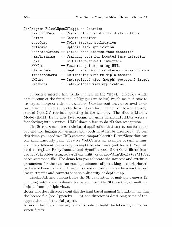
528 Open Source Computer Vision Library Chapter 11
C:\Program Files\OpenCV\apps -- LocationCamShiftDemo -- Track color probability distributionsCommon -- Camera routinescvcsdemo -- Color tracker applicationcvlkdemo -- Optical flow applicationHaarFaceDetect -- Viola-Jones Boosted face detectionHaarTraining -- Training code for Boosted face detectionHawk -- EiC Interpretive C interfaceHMMDemo -- Face recognition using HMMsStereoDemo -- Depth detection from stereo correspondenceTracker3dDemo -- 3D tracking with multiple camerasVMDemo -- Interpolated view (morph) between 2 imagesvmdemotk -- Interpolated view application
Of special interest here is the manual in the “Hawk” directory whichdetails some of the functions in Highgui (see below) which make it easy todisplay an image or video in a window. One line routines can be used to at-tach a menu and/or sliders to the window which can be used to interactivelycontrol OpenCV routines operating in the window. The Hidden MarkovModel (HMM) Demo does face recognition using horizontal HMMs across aface feeding into a vertical HMM down a face to do 2D face recognition.
The StereoDemo is a console-based application that uses cvcam for videocapture and highgui for visualization (both in otherlibs directory). To runthis demo you need two USB cameras compatible with DirectShow that canrun simultaneously pair. Creative WebCam is an example of such a cam-era. Two different cameras types might be also work (not tested). You willneed to register ProxyTrans.ax and SyncFilter.ax DirectShow filters fromopencv\bin folder using regsvr32.exe utility or opencv\bin\RegisterAll.batbatch command file. The demo lets you calibrate the intrinsic and extrinsicparameters for the two cameras by automatically tracking a checkerboardpattern of known size and then finds stereo correspondence between the twoimage streams and converts that to a disparity or depth map.
Tracker3dDemo demonstrates the 3D calibration of multiple cameras (2or more) into one coordinate frame and then the 3D tracking of multipleobjects from multiple views.docs: The docs directory contains the html based manual (index.htm, faq.htm),the license file (see Appendix 11.6) and directories describing some of theapplications and tutorial papers.filters: The filters directory contains code to build the following computervision filters:
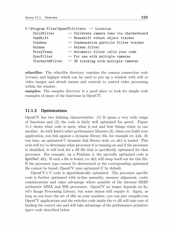
Section 11.1. Overview 529
C:\Program Files\OpenCV\filters -- LocationCalibFilter -- Calibrate camera lens via checkerboardCamShift -- Meanshift robust object trackerCondens -- Condensation particle filter trackerKalman -- Kalman filterProxyTrans -- Automatic filter calls your codeSyncFilter -- For use with multiple camerasTracker3dFilter -- 3D tracking with multiple cameras
otherlibs: The otherlibs directory contains the camera connection code(cvcam) and highgui which can be used to put up a window with still orvideo images and attach menus and controls to control video processingwithin the window.samples: The samples directory is a good place to look for simple codeexamples of many of the functions in OpenCV.
11.1.3 Optimizations
OpenCV has two defining characteristics: (1) It spans a very wide rangeof functions and (2) the code is fairly well optimized for speed. Figure11.1 shows what code is open, what is not and how things relate to oneanother. As with Intel’s other performance libraries [3], when you build yourapplication, you link against a dynamic library file, for example cv.lib. Atrun time, an optimized C dynamic link library stub, cv.dll is loaded. Thisstub will try to determine what processor it is running on and if the processoris identified, it will look for a dll file that is specifically optimized for thatprocessor. For example, on a Pentium 4, the specially optimized code isOptCVw7.dll. If such a file is found, cv.dll will swap itself out for this file.If the processor type cannot be determined or the corresponding optimizedfile cannot be found, OpenCV runs optimized C by default.
OpenCV’s C code is algorithmically optimized. The processor specificcode is further optimized with in-line assembly, memory alignment, cacheconsiderations and takes advantage where possible of the internal SIMDarithmetic MMX and SSE processors. OpenCV no longer depends on In-tel’s Image Processing Library, but some demos still require it. Again, aslong as you have the set of dlls on your machine, you can just compile/runOpenCV applications and the switcher code inside the cv.dll will take care ofloading the correct one and will take advantage of the performance primitiveippcv code described below.
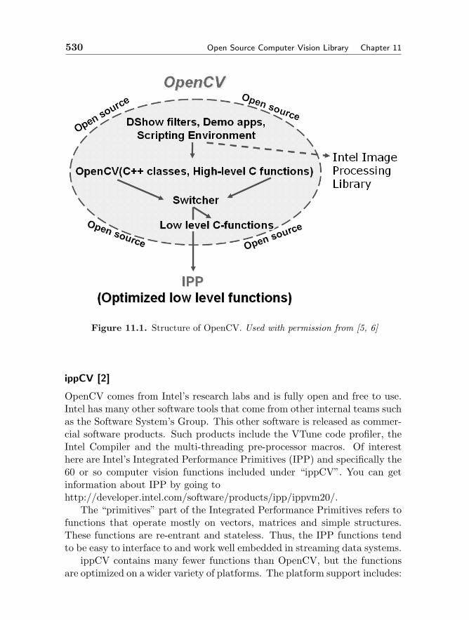
530 Open Source Computer Vision Library Chapter 11
Figure 11.1. Structure of OpenCV. Used with permission from [5, 6]
ippCV [2]
OpenCV comes from Intel’s research labs and is fully open and free to use.Intel has many other software tools that come from other internal teams suchas the Software System’s Group. This other software is released as commer-cial software products. Such products include the VTune code profiler, theIntel Compiler and the multi-threading pre-processor macros. Of interesthere are Intel’s Integrated Performance Primitives (IPP) and specifically the60 or so computer vision functions included under “ippCV”. You can getinformation about IPP by going tohttp://developer.intel.com/software/products/ipp/ippvm20/.
The “primitives” part of the Integrated Performance Primitives refers tofunctions that operate mostly on vectors, matrices and simple structures.These functions are re-entrant and stateless. Thus, the IPP functions tendto be easy to interface to and work well embedded in streaming data systems.
ippCV contains many fewer functions than OpenCV, but the functionsare optimized on a wider variety of platforms. The platform support includes:
Section 11.1. Overview 531
IA32 IntelItanium ArchitectureIntel StrongARM MicroarchitectureIntel XScale Microarchitecture.
Intel IPP supports various operating systems:
32-bit versions of Microsoft Windows64-bit versions of Microsoft Windows MicrosoftWindows CELinux32Linux64ARM Linux.
Inside ippCV, the followig computer vision functions are supported:
Image pyramid (resample & blur)Filters - Laplace, Sobel, Scharr,Erode, DilateMotion gradientFlood fillCanny edge detectionSnakesOptical flow.
Of course, there are many other non-computer vision functions supported in2500 functions that make up IPP. IPP includes support for image processing,compression, signal processing, audio and video codecs, matrix operationsand speech recognition.
Other performance libraries
Two other libraries which serve as higher level wrappers to IPP are of in-terest: The signal processing library and the image processing library [3].OpenCV was designed to work well with both IPP and these libraries. Thefunctions covered by the Signal Processing and Image Processing librariesfollow.
Signal Processing Functions:Data manipulation,windowing,conversion,arithmetic and logical operations
532 Open Source Computer Vision Library Chapter 11
Filters and TransformsStatistics, AudioSignal generation
Image Processing Functions:Data manipulation,arithmetic and logical functions,copy and conversionsGeometric operations (scale, rotate, warp)Color conversion,alpha composite,gamma correctionGeneral and specific filters FFT, DCT, wavelet transform
A final separate library to be aware of is the Math Kernel Library (MKL)which contains the full set of linear algebra and matrix manipulation rou-tines.
11.2 Functional Groups: What’s Good for What
In the Windows directory hierarchy, the OpenCV manual is located atC:\Program Files\OpenCV\docs\index.htm. In the manual, the functionsare broken up into the following groups:
M1. BASIC STRUCTURES AND OPERATIONSHelper structuresArray structuresArrays ManipulationMatrix OperationsDynamic Data StructuresSequencesSetsGraphsWriting and Reading Structures
M2. IMAGE PROCESSING AND ANALYSISDrawing FunctionsGradients,Edges and Corners Sampling,Interpolation and Geometrical TransformsMorphological OperationsFilters and Color Conversion

Section 11.2. Functional Groups: What’s Good for What 533
Pyramids and the ApplicationsConnected componentsImage and contour momentsSpecial Image TransformsHistogram Recognition FunctionsUtility Functions
M3. STRUCTURAL ANALYSISContour Processing FunctionsGeometric Comparison FunctionsPlanar Subdivisions (Triangulation)
M4. MOTION ANALYSIS AND OBJECT TRACKINGAccumulation of Background StatisticsMotion TemplatesObject TrackingOptical FlowEstimators: Kalman, Condensation
M5. OBJECT RECOGNITIONEigen Objects (PCA)Hidden Markov Models
M6. CAMERA CALIBRATION AND 3D RECONSTRUCTIONM7. EXPERIMENTAL FUNCTIONALITY
Statistical BoostingStereo Correspondence3D Tracking with Multiple Cameras
M8. GUI AND VIDEO ACQUISITIONEasy User Interface CreationImage I/O, display and converstionVideo I/O functionsWaitKey/Init system/AddSearchPath
M9. BIBLIOGRAPHYM10. CVCAM CAMERA I/O MANUAL
Exit CameraGetCamerasCountGetPropertyInitPausePlayAVIResumeSelectCameraSetProperty
534 Open Source Computer Vision Library Chapter 11
StartStop
In the next subsection (11.2.1), we will first give an overview of the functionsby area in the manual. In the following subsection (11.2.2) we will give somebrief ideas of what function might be good for what task. A final subsection(11.2.3) discusses what’s in the demos and sample code.
11.2.1 By Area
Below, “M#” refers to the manual sections outlined above.
M1: Structures and Matrices
The first section of the manual begins by describing structures for represent-ing sub-pixel accurate points and rectangles. This is followed by array andimage structures and functions for creating, releasing, copying, setting andother data manipulations of vector or matrix data. Image and matrix logic,arithmetic and conversion are unified and described here along with basicstatistical measures such as sums, averages, STD, mins, maxs and norms.
OpenCV contains a full set of linear algebra routines optimized for smalland typical image sized matrices. Examples of these functions are ma-trix multiplication, dot products, cross products, transpose, inversion, SVD,Eigen images, covariance, Mahalanobis distance, matrix log, power and expo-nential, Cartesian to Polar conversion and back along with random matrices.
Dynamic structures such as linked lists, queues and sets designed to workwith images are described. There are also a full set of Graph and Treestructures such as support Delaunay triangulation. This chapters ends withfunctions that support reading and writing of structures.
M2 Image Processing
The second chapter of the manual covers a wide variety of image processingand analysis routines. It starts off with a basic set of line, conic, poly and textdrawing routines which were included to help in real time labeling and debug.Next, gradient, edge finding and corner detection routines are described.OpenCV allows some useful sampling functions such as reading pixels froman arbitrary line in an image into a vector, or extracting a sub-pixel accuraterectangle or quadrangle (good for rotation) from an image.
A full set of Morphological operations [37] on image objects are sup-ported along with other basic image filtering, thresholding, integral (progres-sive sum images) and color conversion routines. These are joined by image
Section 11.2. Functional Groups: What’s Good for What 535
pyramids, connected components, standard and gradient directed flood fills.For rapid processing, one may find and process gray level or binary contoursof an image object.
A full range of moment processing routines are supported including nor-mal, spatial, central, normalized central and Hu moments [23]. Hough [26]and distance transforms are also present.
In computer vision, histograms of objects have been found very useful forfinding, tracking and identifying objects, including deforming and articulat-ing objects. OpenCV provides a large number of these types of operationssuch as creating, releasing, copying, setting, clearing, thresholding and nor-malizing multi-dimensional histograms. Statistical operations on histogramsare allowed and most of the ways of comparing two histograms to each otherare supported such as correlation, Chi-Square, Intersection [38, 35] andEarth Mover’s distance [34, 33, 32]. Pair-wise geometrical histograms arecovered in manual section M3.. In addition, you can turn histograms intoprobability densities and project images into these probability spaces foranalysis and tracking. The chapter ends with support for most of the ma-jor methods of comparing a template to image regions such as normalizedcross-correlation absolute difference etc.
M3: Structural Analysis
Once grey or binary level image object contours are found (see subsectionM2 above) there are many operations that allow you to smooth, simplifyand compare contours between objects. These contour routines allow rapidfinding of polynomial approximations to objects, bounding boxes, area ofobjects, boundary lengths and shape matching.
Image geometry routines allow one to fit lines, boxes, minimum enclosingcircles and ellipses to data points. This is where you’ll find routines likeKMeans, convex hulls and convexity defect analysis along with minimumarea rotated rectangles. Also in this manual section is support for 2D pair-wise geometrical histograms as described in [24]. This chapter ends withroutines that give full support to Delaunay triangulation.
M4: Motion analysis and tracking
This chapter starts with support for learning the background of a visual scenein order to segment objects by background differencing. Objects segmentedby this method, or any other method may then be tracked by convertingsuccessive segmentations over time into a Motion History image (MHI) [17,13]. Routines can take the gradient of MHIs to further find global and
536 Open Source Computer Vision Library Chapter 11
segmented motion regions.The chapter then moves on to object tracking, first covering tracking of
probability regions in images via the MeanShift and CamShift algorithms[11]. Tracking by energy minimizing Snakes [27] is also supported. Next, 4methods of tracking by optical flow are discussed using Horn and Schunck’salgorithm [22], Lucas and Kanade [30], Block matching, and or recom-mended way, Lucas and Kanade in Image Pyramids [8].
This chapter concludes with two key tracking algorithms, Kalman Filterand Condensation Tracker based on particle filtering. There is an excellenttutorial on Kalman tracking at [41]. For Condensation seehttp://www.dai.ed.ac.uk/CVonline/LOCAL COPIES/ISARD1/condensation.html
M5: Object Recognition
This chapter covers two key techniques in object recognition, Eigen objectsand hidden Markov Models (HMMs). There are many other recognitiontechniques in OpenCV however from Histogram intersection [36] in M2 toBoosted classifers in M7. The HMMs in this section allow HMMs to feed intoother HMMs. One of the OpenCV demos uses horizontal HMMs feeding intoa vertical HMM, termed “embedded HMM” (eHMM), to recognize faces.
M6: Camera Calibration and 3D
OpenCV supports a full set of functions for doing intrinsic (internal cameraparameters and lens distortions) and extrinsic (cameras location with respectto the outside world or other cameras) camera calibration. After calibration,one may then call functions to un-distort a lens or to track objects in 3D (seebelow). Most of these techniques were developed in [43, 45, 44, 21, 10, 9],but we added routines for finding and tracking checkerboard corners in orderto help fill the matrices needed for calibration. In addition, there are routinesfor calculating the homography matrix, finding the fundamental matrix andfinding the epipolar lines between two images. Using calibrated, epipolaraligned images allows us to do “view morphing”, that is, to synthesize a anew object view as a weighted linear combination of the two existing views.Other techniques for stereo correspondence and multi-camera tracking aresupported in manual chapter M7.
This chapter further supports tracking objects in 3D. One way of doingthis is to track a checkerboard object with a calibrated camera. More generalways of tracking 4 or more non-coplaner points on an object using weak-strong perspective iteration (POSIT algorithm) [18] are detailed.
Section 11.2. Functional Groups: What’s Good for What 537
M7: Recent “Experimental” Routines
The “experimental routines” would better be tilted “recent routines”. Thischapter includes support for AdaBoost for face (or other object) detection.Routines support both boosted learning and recognition of objects. Fol-lowing this are routines for finding stereo correspondence where we tried tocombine the best of the faster methods to get good, dense but fast corre-spondence. Note that to do stereo, you should align the cameras as parallelas possible so that the views cover as much of the same scene as possible.Monocular areas not covered by both cameras can cause shearing when theforeground object moves into the monocular area. Finally, routines support-ing tracking objects using multiple (2 or more) cameras are described.
M8: GUI and Video I/O
This manual section covers image and video input and display from diskor cameras (for Windows or Linux) that are contained in the “HighGUI”library. Windows install places source code for this inC:\Program Files\OpenCV\otherlibs\highgui.
Display is covered first with functions that allow you to put up a windowand display video or images there. You can also attach sliders to the windowwhich can be set to control processing parameters that you set up. Functionssupporting full mouse events are also available to make interacting withimages and video easy. A series of functions follow that handle reading andwriting images to disk as well as common image conversions.
The next part of manual section M8 discusses functions for video I/Ofrom either disk or camera. Writing AVIs may be done with various typesof compression including JPEG and MPEG1.
M9: Bibliography
This manual section contains a short bibliography for OpenCV althoughmany citations are placed directly in the function descriptions themselves.
M10:
This last section of the manual is actually a sub-manual devoted to single ormultiple camera control and capture under Windows or Linux . The libraryfor this under Windows is placed in the directoryC:\Program Files\OpenCV\otherlibs\cvcam
538 Open Source Computer Vision Library Chapter 11
11.2.2 By Task
This section will give an all too brief suggestions of what functions might begood for a few of the popular vision tasks. Note that any of the below mayoperate over multiple scales by using the image pyramid functions describedin manual section M2.Camera Calibration, Stereo Depth Maps Camera calibration is di-rectly supported by OpenCV as discussed in section 11.2.1, M6. There areroutines to track a calibration checkerboard to sub-pixel accuracy and touse these points to find the camera matrix and lens distortion parameters.This may then be used to mathematically un-distort the lens or find theposition of the camera relative to the calibration pattern. Two calibratedcameras may be put into stereo correspondence via a routine to calculate theFundamental matrix and then another routine to find the epipolar lines.
From there, the “experimental section” of the manual, M7 above has fastroutines for computing stereo correspondence and uses the found correspon-dence to calculate a depth image. As stated before, it is best if the camerasare aligned as parallel as possible with as little monocular area left in thescene as possible.Background Subtraction, Learning and Segmentation There are dozensof ways that people have employed to learn a background scene. Since thisis a well used and often effective “hack”, I’ll detail a method even if it is notwell supported by OpenCV. A survey of methods may be found in [39]. Thebest methods are long and short term adaptive. Perhaps the best currentmethod is described in Elgammal et. al’s 2000 paper [19] where not the pixelvalues themselves, but the distribution of differences is adaptively learnedusing Kernel estimators. We suspect that this method could be further im-proved by the use linear predictive adaptive filters, especially Lattice filtersdue to their rapid convergence rates.
Unfortunately, the above techniques are not directly supported in OpenCV.Instead, there are routines for learning mean and variance of each pixel (see“Accumulation of Background Statistics” in manual section M4). Also in-side OpenCV, one could instead use the Kalman filter to track pixel values,but the normal distribution assumption behind the Kalman filter does notfit well with the typical bi-modal distribution of pixel values over time. TheCondensation particle filter may be better at this though at a computationalcost for sampling. Within OpenCV, perhaps the best approach is just to usek-means with 2 or 3 means incrementally adapted over a window of time aseach new pixel value comes in using the same short-long scheme as employedby Elgammal in [19].
Section 11.2. Functional Groups: What’s Good for What 539
Once a background model has been found, a thresholded absolute differ-ence cvAbsDiff of the model with the current frame yields the candidateforeground regions. The candidate regions are indicated in a binary maskimage where “on” = foreground candidate, “off” = definite background.Typically this is a gray scale, 8 bit image so that “on” is a value of 255 and“off” is a value of zero.Connected Components The candidate foreground region image abovewill be noisy, and at he image will be filled with pixel “snow”. To clean itup, spurious single pixels need to be deleted by performing a morpholog-ical erode followed by a morphological dilate operation. This operation iscalled “morphological open” and can be done in one shot using the OpenCVfunction cvMorphologyEx using a 3x3 pixel cross shaped structuring elementusing the enumerated value CV SHAPE CROSS and performing the openoperation using CV MOP OPEN with one iteration.
Next we want to identify and label large connected groups of pixels,deleting anything “too small”. The candidate foreground image is scannedand any candidate foreground pixel (value = 255) found is used as a floodfill seed start point to mark the entire connected region using the OpenCVcvFloodFill function. Each region will be marked by a different number bysetting the cvFloodFill “newVal” to the new fill value. The first found regionis marked with 1, then 2 ... up to a max of 254 regions. In cvFloodFill, thelo and up values should be set to zero, a CvConnectedComp structure shouldbe passed to the function, flags should be set to 8. Once the region is filled,the area of the fill is examined (it is set in CvConnectedComp). If the areafilled is below a minimum area size threshold Tsize, that area is erased byflooding it with a new value of zero newVal = 0 (regions that are too smallare considered noise). If the area was greater than Tsize, then it is kept andthe next fill value incremented subject to it being less than 255.
Getting rid of branch movement, camera jitter
Since moving branches and slight camera movement in the wind can causemany spurious foreground candidate regions, we need a false detection sup-pression routine such as described in pages 6-8 of Elgammal et. al’s paper[19]. Every labeled candidate foreground pixel i has its probability recal-culated by testing the pixel’s value against each of its neighboring pixel’sprobability distribution in a 5x5 region around it N5x5. The maximum back-ground probability calculation is assigned to that foreground pixel:
PN5x5(ix,y(t)) = maxj∈N5x5
P (ix,y(t)|Bj), (11.1)
540 Open Source Computer Vision Library Chapter 11
where Bj is the background sample for the appropriate pixel j in the 5x5neighborhood. If the probability of being background is greater than athreshold TBG1 , then that candidate foreground pixel is labeled as back-ground. But, since this would knock out too many true positive pixels, wealso require that the whole connected region C also be found to be proba-bilistically a part of the background:
PC =∏i∈C
PN5x5(i). (11.2)
A former candidate foreground pixel is thus demoted to background if:
(PN5x5(i) > TBG1) ∧ (PC(i) > TBG2) (11.3)
where TBG1 and TBG2 are suppression thresholds.Stereo Background Subtraction This is much like the above, except weget a depth map from two or more cameras. The basic idea is that youcan also statistically learn the depth background. In detection mode youexamine as foreground only those regions that are in front of your knownbackground. The OpenCV camera calibration and stereo correspondenceroutines are of great help there (Manual sections M6 and M7).People Tracking There are innumerable ways to accomplish this task. Oneapproach is to fit a full physical model to a person in a scene. This tends tobe slow and is not supported in OpenCV and so won’t be discussed further.For multiple cameras, one can look to the experimental section of the man-ual, M7 above where multiple tracked areas are put into 3D correspondence.Other typical methods of tracking whole people are to sample a histogram(M2 Histogram functions) or template (M2 MatchTemplate) from a person,then scan through the future frames back-projecting histogram intersections,earth mover distances or template match scores to create a probability of per-son image. The mean shift or CamShift algorithms (M4) can then track therecognition peaks in these images. Alternatively, people could be representedas a sequence of vertically oriented color blobs as done in [42]. This couldbe accomplished in OpenCV by use of cvKMeans2 described in M3 to clustercolors, or just by using the image statistical functions described in the arraystatistics section of M1, or by using the undocumented texture descriptorsin the experimental section (look for “GLMC” in cvaux.h). A “probabilitiesof match” image can be made this way and tracked by meanshift as above.
Another people tracking approach if you can get adequate background-foreground segmentation is to use the Motion History Templates and MotionGradients as described in manual section M4.
Section 11.2. Functional Groups: What’s Good for What 541
Face Finding and Recognition The good way of doing this is by theViola-Jones method as described in [40] and fully implemented in OpenCV(see section M7 in the manual and the accompanying demo app in the appssection of the OpenCV directory.
Face recognition may be either done through Eigen images or embeddedHidden Markov Models (see manual section M5), both of which have workingdemos in the apps directories.Image Retrieval Image retrieval is typically done via some form of his-togram analysis. This is fully supported via the histogram learning andcomparison functions described in manual section M2.Gesture Recognition for Arcade Perhaps the best way if you can getadequate background-foreground segmentation is to use the Motion HistoryTemplates and Motion Gradients as described in manual section M4. Forrecognition, depending on your representation, you may use the histogramfunctions described in M2, Mahalanobis distances in M1 or do some sort of“Eigen trajectories using Eigen objects in M5. If hand shape is also required,one can represent the hand as a gradient histogram and use the histogramrecognition techniques in M2.
The calibration, stereo and/or 3D tracking routines described in M6 andM7 can also help segment and track motion in 3D. HMMs from section M5can be used for recognition.Part Localization, Factory Applications OpenCV was not built to sup-port factory machine vision applications, but it does have some useful func-tionality. The camera calibration (manual section M6), stereo routines (M7)can help with part segmentation. Templates can be compared with theMatchTemplate function in M2. Lines may be found with the Canny edgedetector or Hough transform in M2.
There are routines for the sub-pixel accurate location of corners, rectan-gles and quadrangles. Where to move can be aided by distance transforms.Adaptive thresholds can help segment parts and Pyramid operations can dothings over multiple scales, all in M2.
Part shapes can be analyzed and recognized through the extensive collec-tion of contour operators in M2. Motion can be analyzed and compensatedfor using optical flow routines in M4. Kalman and Condensation particle fil-ters for smoothing, tracking or predicting motion are supported as describedin M4.Flying a Plane Autonomous or semi-autonomous planes are popular nowfor sport or military applications. It turns out that a plane can be flownknowing only the horizon line. Assume that a camera has been installedsuch that the direction of heading is the exact center of the image and that
542 Open Source Computer Vision Library Chapter 11
level flight corresponds to the horizontal image scan lines being tangent tothe earth’s curvature. It then turns out that knowing the horizon line isenough to fly the plane. The angle of the horizon line is used for roll controland the perpendicular distance from the line to the center of the image tellsthe pitch of the plane.
All we need then is a fast, robust way of finding the horizon line. Asimple heurstic for finding this line was developed by Scott Ettinger [20].Basically, we find the line through the image that minimizes the varianceon both sides of the line (sky is more like sky than ground and vice versa).This may be simply done every frame by creating an image pyramid (inmanual section M2) of the aerial scene. On a much reduce scale image findthe variance above and below the horizontal line through the center of theimage using image (Array) statistics (M1). We then systematically moveand rotate the line until variance is minimized on both sides of the line. Wecan then advance to a larger or full scale to refine the line angle and location.Note that every time we move the line, we need not re-calculate the variancefrom scratch. Rather, as points enter a side, their sum is added to that sidesvariance and lost points are subtracted.OCR The Hough transform (HoughLines) for lines in manual section M2 canbe used to find the dominant orientation of text on a page. The machineryused for statistically boosted face finding described in M7 could also be usedfor either finding individual letters, or finding and recognizing the letters.The Russian team created extremely fast letter recognition by thresholdingletters, finding contours (cvFindContours M2), simplifying the contours rep-resenting the contours as trees of nested regions and holes, and matching thetrees as described in the Contour Processing Functions in M3.
The author has had quite good results from using the embedded HiddenMarkov Model recognition techniques described in manual section M5 ontext data. There are demos for both these routines (but applied to faces nottext) included in the apps directory of OpenCV.
11.2.3 Demos and Samples
The demo applications that ship with OpenCV are:
CamShiftDemo, cvcsdemo
This is a statistically robust probability distribution mode tracker. It isbased on making the tracking window of the mean shift algorithm dynamic– this supports visual objects that can resize themselves by moving withinhe visual field. But due to this, if your probability distributions are not
Section 11.2. Functional Groups: What’s Good for What 543
compact (e.g. if they diffuse all over the image), CamShift will not work andyou should switch to just Meanshift. For the demo, the distribution thatCamShift tracks is just the probability of color that you selected from thevideo stream of images.
CamShiftDemo is the same as cvcsdemo, just using a tcl interface.
LKDemo, cvlkdemo
This is a real time Lucas-Kanade in image pyramid tracking demo. Notethat Lucas-Kanade is a window based tracker and windows are ambiguousat object boundaries. Thus, windows on a boundary may tend to slide orstick to the the background or foreground interior. The LKDemo is the sameas cvlkdemo, the later just uses a tcl interface.
HaarFaceDetect, HaarTraining
This is a slight modification to Viola-Jones AdaBoost Face detector whichused Haar type waveletts as weak feature detectors. Training code (butnot the raw face database), trained parameters and working real time facedetection are included here.
Hawk
Hawk is a window based interactive C scripting system for working withOpenCV functions. It uses EiC interpretive C as its engine – some of High-GUI grew out of this. See other interfaces, Section 11.5 below for what hasreplaced this earlier interface.
HMMDemo
This is a working HMM based face detection demo complete with a sampledatabase to train on2. This demo has HMMs across the face feeding into avertical HMM down the face which makes the final decision. You may add tothe database by live camera. The HMM technique works well except we giveit uniform priors (uniformly cut up the image) to initialize training. If facesare not precisely aligned, the facial features will be blurred. This structuralblurring leaves lighting as a stronger, though accidental, feature and so thisapplication tends to be lighting sensitive. Putting in actual eye, nose, mouthpriors into the model would probably minimize lighting dependence, but wehave not tried this yet.
2Some early members of the Russian OpenCV development team form the trainingdatabase images.
544 Open Source Computer Vision Library Chapter 11
StereoDemo
This is a console-based stereo depth calculation application that uses cvcamfor video capture and highgui for displaying the images. See the readme filein ...\apps \StereoDemo for how to run this application. You will need twoUSB cameras that are compatible with DirectShow that can run together.Creative WebCam is an example of such a camera. Two different camerasmight be also OK.
This application allows automatic calibration of the cameras via trackinga checkerboard and then running to develop the disparity/depth image.
Tracker3dDemo
This demo uses 2 or more cameras calibrated together to track blobs in 3D.
VMDemo, vmdemotk
This demo, complete with sample images in the Media subdirectory uses theepipolar lines between two calibrated views to morph (interpolate) cameraviews anywhere between two views of an object. VMDemo and vmdemotkare the same except that the later uses tcl and the former uses direct showfilters.
Sample Code
On the Windows install, the sample code can be found at:C:\Program Files\OpenCV\samples\c. The same directory also containssome test images that the some of the sample code operates on.
The sample codes are just simple examples of use of the following rou-tines:
squares.c -- Uses contours to find colored rotated squares.pyramid_segmentation.c -- Uses image pyramids for color segmentation.motempl.c -- Using motion templates to track motionmorphology.c -- Uses morphological operators.laplace.c -- Use of laplace operator on image.kmeans.c -- Find clusters by K-Means algorithm.kalman.c -- Track by the Kalman filter.fitellipse.c -- Best fit of ellipse to data.ffilldemo.c -- Use of flood fill.facedetect.c -- Uses AdaBoost based face detector.edge.c -- Uses Canny operator to edges in an image.drawing.c -- Demos the drawing functions.distrans.c -- Demos the distance transform function.DemHist.c -- Demos use of several of the Histogram functions.
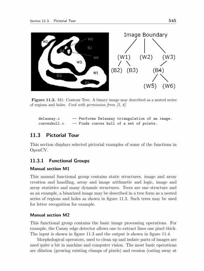
Section 11.3. Pictorial Tour 545
Figure 11.2. M1: Contour Tree. A binary image may described as a nested seriesof regions and holes. Used with permission from [5, 6]
delaunay.c -- Performs Delaunay triangulation of an image.convexhull.c -- Finds convex hull of a set of points.
11.3 Pictorial Tour
This section displays selected pictorial examples of some of the functions inOpenCV.
11.3.1 Functional Groups
Manual section M1
This manual functional group contains static structures, image and arraycreation and handling, array and image arithmetic and logic, image andarray statistics and many dynamic structures. Trees are one structure andas an example, a binarized image may be described in a tree form as a nestedseries of regions and holes as shown in figure 11.2. Such trees may be usedfor letter recognition for example.
Manual section M2
This functional group contains the basic image processing operations. Forexample, the Canny edge detector allows one to extract lines one pixel thick.The input is shown in figure 11.3 and the output is shown in figure 11.4.
Morphological operators, used to clean up and isolate parts of images areused quite a bit in machine and computer vision. The most basic operationsare dilation (growing existing clumps of pixels) and erosion (eating away at
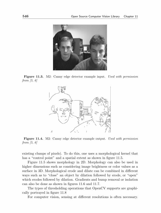
546 Open Source Computer Vision Library Chapter 11
Figure 11.3. M2: Canny edge detector example input. Used with permissionfrom [5, 6]
Figure 11.4. M2: Canny edge detector example output. Used with permissionfrom [5, 6]
existing clumps of pixels). To do this, one uses a morphological kernel thathas a “control point” and a spatial extent as shown in figure 11.5.
Figure 11.5 shows morphology in 2D. Morphology can also be used inhigher dimensions such as considering image brightness or color values as asurface in 3D. Morphological erode and dilate can be combined in differentways such as to “close” an object by dilation followed by erode, or “open”which erodes followed by dilation. Gradients and bump removal or isolationcan also be done as shown in figures 11.6 and 11.7.
The types of thresholding operations that OpenCV supports are graphi-cally portrayed in figure 11.8
For computer vision, sensing at different resolutions is often necessary.
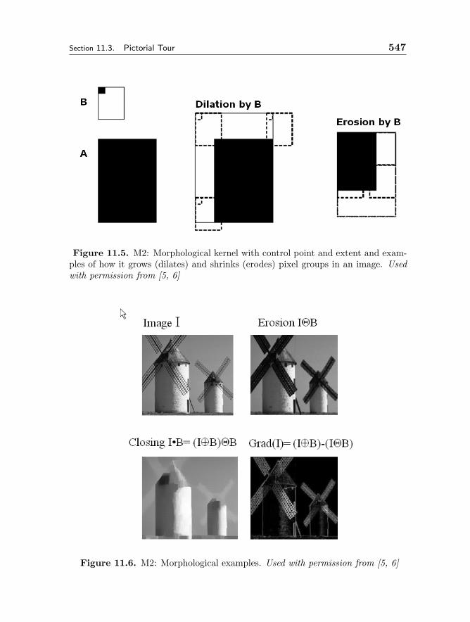
Section 11.3. Pictorial Tour 547
Figure 11.5. M2: Morphological kernel with control point and extent and exam-ples of how it grows (dilates) and shrinks (erodes) pixel groups in an image. Usedwith permission from [5, 6]
Figure 11.6. M2: Morphological examples. Used with permission from [5, 6]

548 Open Source Computer Vision Library Chapter 11
Figure 11.7. M2: More morphological examples. Used with permission from [5, 6]
Figure 11.8. M2: OpenCV image threshold options. Used with permissionfrom [5, 6]

Section 11.3. Pictorial Tour 549
Figure 11.9. M2: Scale and Laplacian image pyramids. Used with permissionfrom [5, 6]
OpenCV comes with an image pyramid or Laplacian pyramid function asshown in figure 11.9.
Flood fill is a graphics operator that is also used in computer vision forlabeling regions as belonging together. OpenCV’s floodfill can additionallyfill upwards or downwards. Figure 11.10 shows an example of flood filling.
In addition to Canny edge detector, one often wants to find dominantstraight lines in an image even if there might be discontinuities in those lines.The Hough transform is a robust method of finding dominant straight linesin an image. In figure 11.11 we have the raw image of a building and figure11.12 shows the dominant lines found by the Hough transform.
The final example we’ll show from chapter M2 is Borgefors’ distancetransform [7]. The distance transform calculates the approximate distancefrom every binary image pixel to the nearest zero pixel. This is shown in
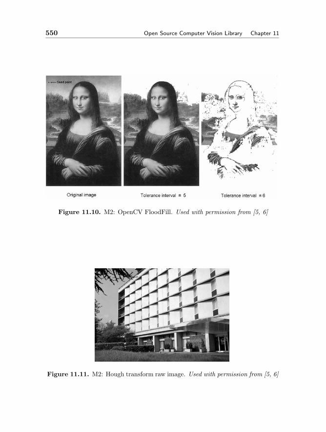
550 Open Source Computer Vision Library Chapter 11
Figure 11.10. M2: OpenCV FloodFill. Used with permission from [5, 6]
Figure 11.11. M2: Hough transform raw image. Used with permission from [5, 6]
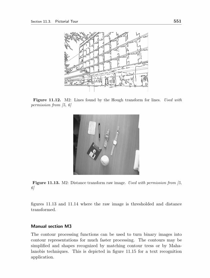
Section 11.3. Pictorial Tour 551
Figure 11.12. M2: Lines found by the Hough transform for lines. Used withpermission from [5, 6]
Figure 11.13. M2: Distance transform raw image. Used with permission from [5,6]
figures 11.13 and 11.14 where the raw image is thresholded and distancetransformed.
Manual section M3
The contour processing functions can be used to turn binary images intocontour representations for much faster processing. The contours may besimplified and shapes recognized by matching contour tress or by Maha-lanobis techniques. This is depicted in figure 11.15 for a text recognitionapplication.
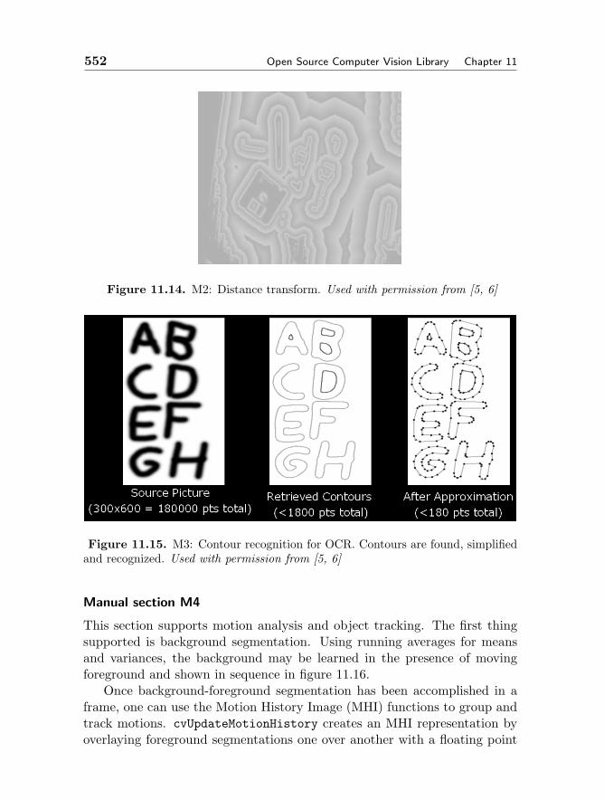
552 Open Source Computer Vision Library Chapter 11
Figure 11.14. M2: Distance transform. Used with permission from [5, 6]
Figure 11.15. M3: Contour recognition for OCR. Contours are found, simplifiedand recognized. Used with permission from [5, 6]
Manual section M4
This section supports motion analysis and object tracking. The first thingsupported is background segmentation. Using running averages for meansand variances, the background may be learned in the presence of movingforeground and shown in sequence in figure 11.16.
Once background-foreground segmentation has been accomplished in aframe, one can use the Motion History Image (MHI) functions to group andtrack motions. cvUpdateMotionHistory creates an MHI representation byoverlaying foreground segmentations one over another with a floating point
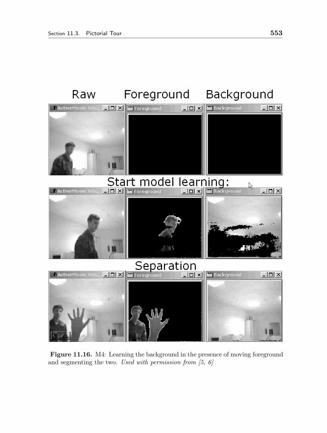
Section 11.3. Pictorial Tour 553
Figure 11.16. M4: Learning the background in the presence of moving foregroundand segmenting the two. Used with permission from [5, 6]
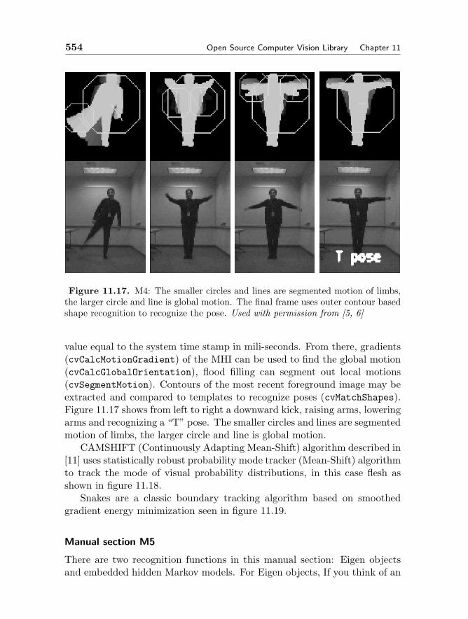
554 Open Source Computer Vision Library Chapter 11
Figure 11.17. M4: The smaller circles and lines are segmented motion of limbs,the larger circle and line is global motion. The final frame uses outer contour basedshape recognition to recognize the pose. Used with permission from [5, 6]
value equal to the system time stamp in mili-seconds. From there, gradients(cvCalcMotionGradient) of the MHI can be used to find the global motion(cvCalcGlobalOrientation), flood filling can segment out local motions(cvSegmentMotion). Contours of the most recent foreground image may beextracted and compared to templates to recognize poses (cvMatchShapes).Figure 11.17 shows from left to right a downward kick, raising arms, loweringarms and recognizing a “T” pose. The smaller circles and lines are segmentedmotion of limbs, the larger circle and line is global motion.
CAMSHIFT (Continuously Adapting Mean-Shift) algorithm described in[11] uses statistically robust probability mode tracker (Mean-Shift) algorithmto track the mode of visual probability distributions, in this case flesh asshown in figure 11.18.
Snakes are a classic boundary tracking algorithm based on smoothedgradient energy minimization seen in figure 11.19.
Manual section M5
There are two recognition functions in this manual section: Eigen objectsand embedded hidden Markov models. For Eigen objects, If you think of an
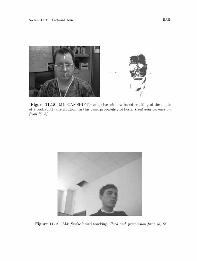
Section 11.3. Pictorial Tour 555
Figure 11.18. M4: CAMSHIFT – adaptive window based tracking of the modeof a probability distribution, in this case, probability of flesh. Used with permissionfrom [5, 6]
Figure 11.19. M4: Snake based tracking. Used with permission from [5, 6]
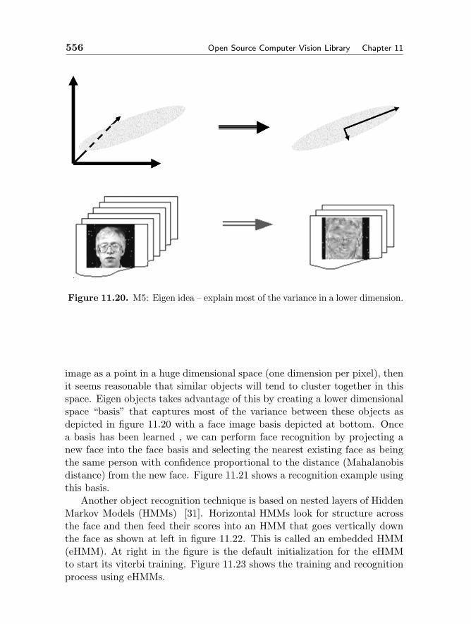
556 Open Source Computer Vision Library Chapter 11
Figure 11.20. M5: Eigen idea – explain most of the variance in a lower dimension.
image as a point in a huge dimensional space (one dimension per pixel), thenit seems reasonable that similar objects will tend to cluster together in thisspace. Eigen objects takes advantage of this by creating a lower dimensionalspace “basis” that captures most of the variance between these objects asdepicted in figure 11.20 with a face image basis depicted at bottom. Oncea basis has been learned , we can perform face recognition by projecting anew face into the face basis and selecting the nearest existing face as beingthe same person with confidence proportional to the distance (Mahalanobisdistance) from the new face. Figure 11.21 shows a recognition example usingthis basis.
Another object recognition technique is based on nested layers of HiddenMarkov Models (HMMs) [31]. Horizontal HMMs look for structure acrossthe face and then feed their scores into an HMM that goes vertically downthe face as shown at left in figure 11.22. This is called an embedded HMM(eHMM). At right in the figure is the default initialization for the eHMMto start its viterbi training. Figure 11.23 shows the training and recognitionprocess using eHMMs.
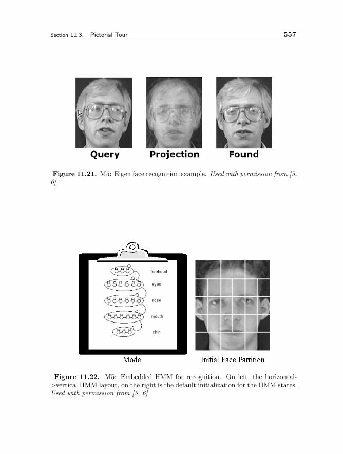
Section 11.3. Pictorial Tour 557
Figure 11.21. M5: Eigen face recognition example. Used with permission from [5,6]
Figure 11.22. M5: Embedded HMM for recognition. On left, the horizontal->vertical HMM layout, on the right is the default initialization for the HMM states.Used with permission from [5, 6]
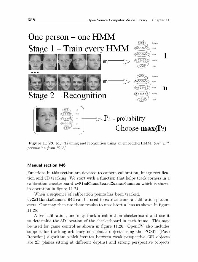
558 Open Source Computer Vision Library Chapter 11
Figure 11.23. M5: Training and recognition using an embedded HMM. Used withpermission from [5, 6]
Manual section M6
Functions in this section are devoted to camera calibration, image rectifica-tion and 3D tracking. We start with a function that helps track corners in acalibration checkerboard cvFindChessBoardCornerGuesses which is shownin operation in figure 11.24.
When a sequence of calibration points has been tracked,cvCalibrateCamera_64d can be used to extract camera calibration param-eters. One may then use these results to un-distort a lens as shown in figure11.25.
After calibration, one may track a calibration checkerboard and use itto determine the 3D location of the checkerboard in each frame. This maybe used for game control as shown in figure 11.26. OpenCV also includessupport for tracking arbitrary non-planar objects using the POSIT (PoseIteration) algorithm which iterates between weak perspective (3D objectsare 2D planes sitting at different depths) and strong perspective (objects
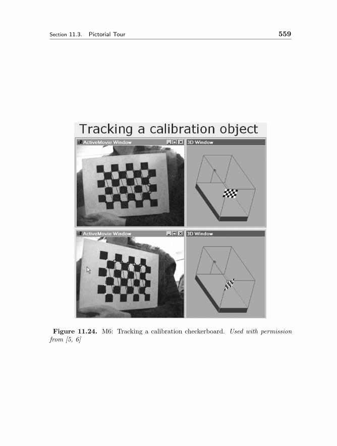
Section 11.3. Pictorial Tour 559
Figure 11.24. M6: Tracking a calibration checkerboard. Used with permissionfrom [5, 6]
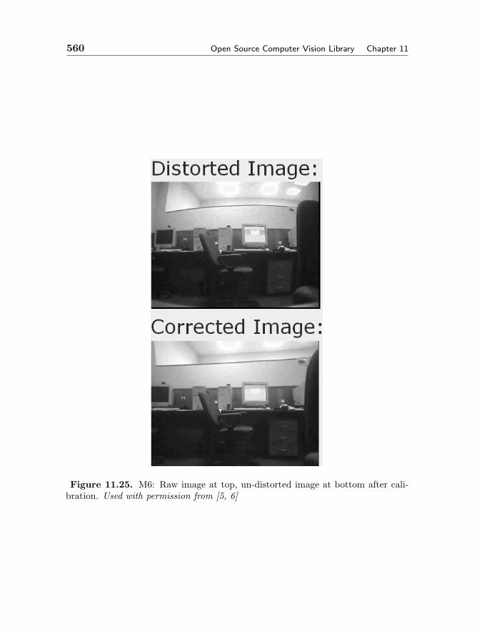
560 Open Source Computer Vision Library Chapter 11
Figure 11.25. M6: Raw image at top, un-distorted image at bottom after cali-bration. Used with permission from [5, 6]
Section 11.4. Programming Examples Using C/C++ 561
are 3D) interpretation of points on objects. With mild constraints, POSITrapidly converges to the true 3D object pose which may also be used to track3D objects.
Not shown here, but in the experimental manual section M7 are functionsthat further use calibrated cameras for stereo vision and 3D Modeling. Wenext pictorially describe some of the demos that ship with OpenCV.
11.3.2 Demo Tour
This subsection shows some images of some of the demos that ship withOpenCV. Not shown is our version [28] of the Viola-Jones face tracker [40],and also not shown is the 2-video camera stereo demo. Shown below arescreen shots of the Calibration demo and the control screen for the multiplecamera 3D tracking experimental demo in figure 11.27. Also shown are colorbased tracking using CAMSHIFT, Kalman Filter and Condensation in figure11.28. Figure 11.29 shows the HMM based face recognition demo (also goodfor letter recognition) and finally optical flow in figure 11.30.
11.4 Programming Examples Using C/C++
Windows setup tips:
To get programs to compile in MSVC++, there are some things you mustdo.
– release or debug mode. MSVC++ can make either release or debugcode. OpenCV ships with only release code (you can build debugyourself). If a link error comes up requesting “cvd.lib” you are indebug mode. Go to the Build menu, select Set Active Configurationand set it to release code.
– Include and Library file paths must be set. Go to the Tools menu,select Options. Click on the Directories tab. Under “Show Directoriesfor”, select Include files. Set the include path for
C:\Program Files\OpenCV\cv\includeC:\Program Files\OpenCV\cvaux\includeC:\Program Files\OpenCV\otherlibs\cvcam\includeC:\Program Files\OpenCV\otherlibs\highgui
Next, select Library files and set the path for C:\Program Files\OpenCV\lib.
– To avoid “unreferenced” function errors in link, go to Project, selectSettings and click on the Link tab. Under “Object/library modules”add cv.lib cvcam.lib highgui.lib.

562 Open Source Computer Vision Library Chapter 11
Figure 11.26. M6: Tracking a 3D object for game control. Used with permissionfrom [5, 6]

Section 11.4. Programming Examples Using C/C++ 563
Calibration Demo:
Multi-Camera 3D Tracking:
Figure 11.27. Demos: Automatic checkerboard tracking for camera calibrationabove and control screen for multiple camera 3D below. Used with permissionfrom [5, 6]
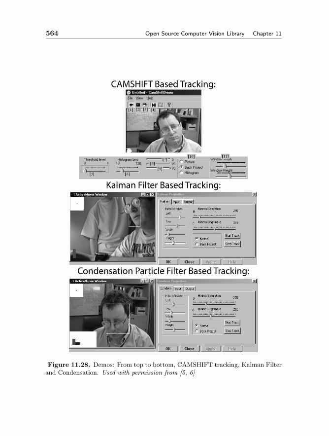
564 Open Source Computer Vision Library Chapter 11
Condensation Particle Filter Based Tracking:
Kalman Filter Based Tracking:
CAMSHIFT Based Tracking:
Figure 11.28. Demos: From top to bottom, CAMSHIFT tracking, Kalman Filterand Condensation. Used with permission from [5, 6]
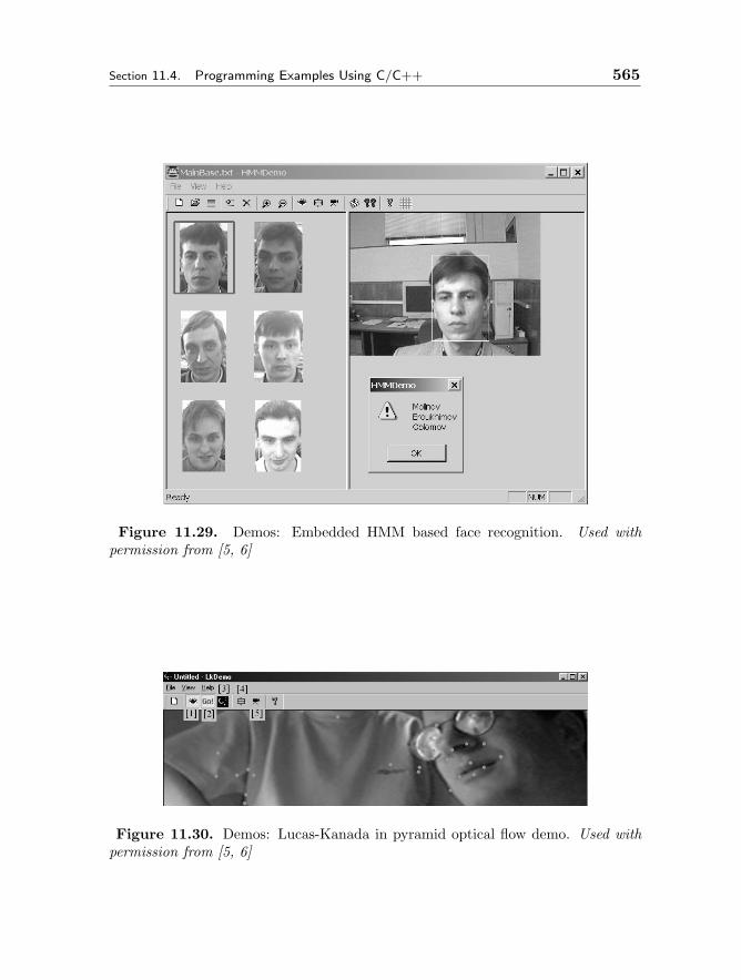
Section 11.4. Programming Examples Using C/C++ 565
Figure 11.29. Demos: Embedded HMM based face recognition. Used withpermission from [5, 6]
Figure 11.30. Demos: Lucas-Kanada in pyramid optical flow demo. Used withpermission from [5, 6]

566 Open Source Computer Vision Library Chapter 11
– Finally, make sure the windows path has C:\Program Files\OpenCV\binin it and that you’ve run RegisterAll.bat there at least once.
11.4.1 Read Images from Disk
The program below reads an image from disk (either from the commandline or “Mface.jpg” by default) and performs pyramid based color regionsegmentation controlled by two interactive sliders. The input and outputalong with slider controls is shown in figure 11.31.
#ifdef _CH_#pragma package <opencv>#endif
#ifndef _EiC#include "cv.h"#include "highgui.h"#include <math.h>#endifIplImage* image[2] = 0, 0 , *image0 = 0, *image1 = 0;CvSize size;int w0, h0,i;int threshold1, threshold2;int l,level = 4;int sthreshold1, sthreshold2;int l_comp;int block_size = 1000;float parameter;double threshold;double rezult, min_rezult;CvFilter filter = CV_GAUSSIAN_5x5;CvConnectedComp *cur_comp,min_comp;CvSeq *comp;CvMemStorage *storage;CvPoint pt1, pt2;
void ON_SEGMENT(int a) cvPyrSegmentation(image0, image1, storage, &comp,
level, threshold1, threshold2);l_comp = comp->total;i = 0;min_comp.value = 0;while(i<l_comp)
cur_comp = (CvConnectedComp*)cvGetSeqElem ( comp, i, 0);

Section 11.4. Programming Examples Using C/C++ 567
if(fabs(CV_RGB(255,0,0)- min_comp.value)>fabs(CV_RGB(255,0,0)- cur_comp->value))min_comp = *cur_comp;
i++;cvShowImage("Segmentation", image1);
int main( int argc, char** argv ) char* filename = argc == 2 ? argv[1] : (char*)"Mface.jpg";if( (image[0] = cvLoadImage( filename, 1)) == 0 )
return -1;cvNamedWindow("Source", 0);cvShowImage("Source", image[0]);cvNamedWindow("Segmentation", 0);storage = cvCreateMemStorage ( block_size );image[0]->width &= -(1<<level);image[0]->height &= -(1<<level);image0 = cvCloneImage( image[0] );image1 = cvCloneImage( image[0] );// segmentation of the color imagel = 1;threshold1 =255;threshold2 =30;ON_SEGMENT(1);sthreshold1 = cvCreateTrackbar("Threshold1", "Segmentation",
&threshold1, 255, ON_SEGMENT);sthreshold2 = cvCreateTrackbar("Threshold2", "Segmentation",
&threshold2, 255, ON_SEGMENT);cvShowImage("Segmentation", image1);cvWaitKey(0);cvDestroyWindow("Segmentation");cvDestroyWindow("Source");cvReleaseMemStorage(&storage );cvReleaseImage(&image[0]);cvReleaseImage(&image0);cvReleaseImage(&image1);return 0;
#ifdef _EiC main(1,"pyramid_segmentation.c");#endif
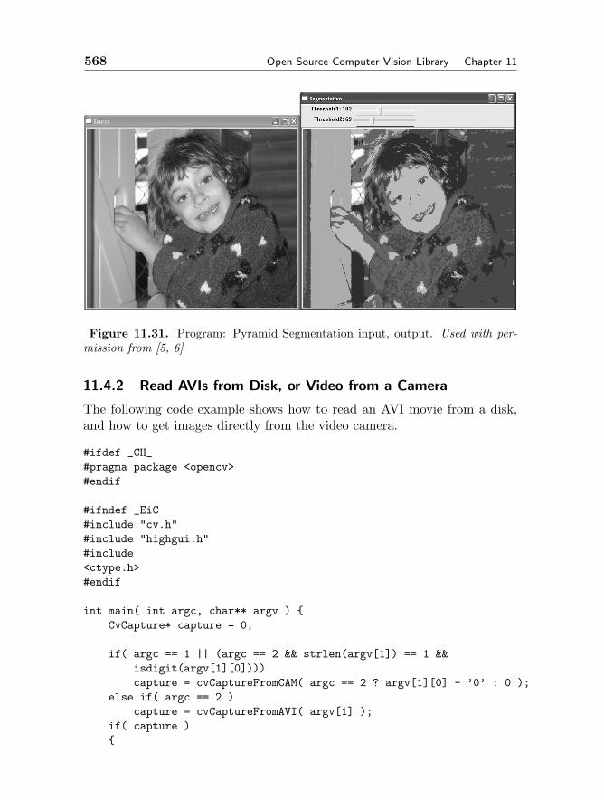
568 Open Source Computer Vision Library Chapter 11
Figure 11.31. Program: Pyramid Segmentation input, output. Used with per-mission from [5, 6]
11.4.2 Read AVIs from Disk, or Video from a Camera
The following code example shows how to read an AVI movie from a disk,and how to get images directly from the video camera.
#ifdef _CH_#pragma package <opencv>#endif
#ifndef _EiC#include "cv.h"#include "highgui.h"#include<ctype.h>#endif
int main( int argc, char** argv ) CvCapture* capture = 0;
if( argc == 1 || (argc == 2 && strlen(argv[1]) == 1 &&isdigit(argv[1][0])))capture = cvCaptureFromCAM( argc == 2 ? argv[1][0] - ’0’ : 0 );
else if( argc == 2 )capture = cvCaptureFromAVI( argv[1] );
if( capture )
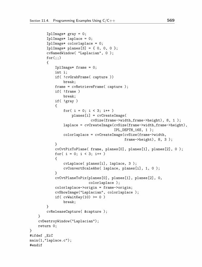
Section 11.4. Programming Examples Using C/C++ 569
IplImage* gray = 0;IplImage* laplace = 0;IplImage* colorlaplace = 0;IplImage* planes[3] = 0, 0, 0 ;cvNamedWindow( "Laplacian", 0 );for(;;)
IplImage* frame = 0;int i;if( !cvGrabFrame( capture ))
break;frame = cvRetrieveFrame( capture );if( !frame )
break;if( !gray )
for( i = 0; i < 3; i++ )planes[i] = cvCreateImage(
cvSize(frame->width,frame->height), 8, 1 );laplace = cvCreateImage(cvSize(frame->width,frame->height),
IPL_DEPTH_16S, 1 );colorlaplace = cvCreateImage(cvSize(frame->width,
frame->height), 8, 3 );cvCvtPixToPlane( frame, planes[0], planes[1], planes[2], 0 );for( i = 0; i < 3; i++ )
cvLaplace( planes[i], laplace, 3 );cvConvertScaleAbs( laplace, planes[i], 1, 0 );
cvCvtPlaneToPix(planes[0], planes[1], planes[2], 0,
colorlaplace );colorlaplace->origin = frame->origin;cvShowImage("Laplacian", colorlaplace );if( cvWaitKey(10) >= 0 )
break;cvReleaseCapture( &capture );
cvDestroyWindow("Laplacian");return 0;
#ifdef _EiCmain(1,"laplace.c");#endif
570 Open Source Computer Vision Library Chapter 11
11.5 Other Interfaces
There are other ways to “talk” to OpenCV beyond compiled C. We detailthree main methods below: Ch, Matlab and Lush.
11.5.1 Ch
What is Ch?
Ch is a superset of C interpreter. It is designed for cross- platform scripting,2D/3D plotting and numerical computing. Ch was originally designed andimplemented by Harry H. Cheng [16]. It has been further developed andmaintained by SoftIntegration, Inc. [15, 25]
Ch supports 1999 ISO C Standard (C99), classes in C++, POSIX, X11/Motif,OpenGL, ODBC, XML, GTK+, Win32, CGI, 2D/3D graphical plotting,socket/Winsock, C LAPACK, high level numeric functions, and shell pro-gramming.
The extensions in Ch provide the simplest possible solution for numeri-cal computing and visualization in C/C++ domain. Ch can interface withC/C++ binary libraries and be embedded in other application programs andhardware.
What is Ch OpenCV Package
Ch OpenCV package is Ch binding to OpenCV. Ch OpenCV package isincluded in the distribution of OpenCV. With Ch OpenCV, C (or C++)programs using OpenCV C functions can readily run in Ch without compila-tion. Both Ch Standard/Professional/Student Edition and OpenCV runtimelibrary are needed to run Ch OpenCV.
Contents of Ch OpenCV Package
Ch OpenCV package contains the following directories
1. OpenCV - Ch OpenCV package
– OpenCV/demos — OpenCV demo programs in C readily to runin Ch
– OpenCV/bin — OpenCV dynamical library and commands
– OpenCV/dl — dynamically loaded library
– OpenCV/include — header files
– OpenCV/lib — function files

Section 11.5. Other Interfaces 571
2. Devel - Files and utilities used to build Ch OpenCV package usingnative C compiler and Ch SDK
– Devel/c — chdl.c C wrappers and Makefile’s
– Devel/createchf — bare OpenCV headers
– Devel/include — Ch OpenCV-specific include files
Where to get Ch and Setup Ch OpenCV
Ch OpenCV can be installed in your computer following instruction below.Here we assume <CHHOME> is the directory where Ch is installed, forexample if Ch is installed in C:/Ch, then C:/Ch should be used instead of<CHHOME>. We also assume <OPENCV HOME> is the directory whereOpenCV is installed. For example, if OpenCV is installed in C:/ProgramFiles/OpenCV, then <OPENCV HOME> should also be substituted byC:/Program Files/OpenCV.
1. If Ch has not been installed in your computer, download and installCh from http://www.softintegration.com
2. Move the directory OpenCV to <CHHOME>/package/opencv.<CHHOME>/package/opencv becomes the home directory ofCHOPENCV HOME for Ch OpenCV package. If you do not wantto move the directory, you should add a new path to the systemvariable ppath for package path by adding the following statementin system startup file <CHHOME> /config/chrc or individual user’sstartup file chrc in the user’s home directory ppath = stradd( ppath,“<OPENCV HOME> /interfaces/ch;”); <OPENCV HOME> /inter-faces/ch/ opencv becomes the home directory CHOPENCV HOMEfor Ch OpenCV package.
3. Add the system variable ipath in system startup file indicated in theprevious step by adding the following statement. ipath = stradd( ipath,“<CHOPENC V HOME> /include;”); This step will not be necessaryif the following code fragment is in application programs.
#ifdef _CH_#pragma package <opencv>
#endif

572 Open Source Computer Vision Library Chapter 11
Run Demo Programs in Directory demos:
1. start ch
2. type program name such as ’delaunay.c’
Update Ch OpenCV Package for Newer Versions of OpenCV
As discussed above how to integrate Ch and OpenCV, the update of ChOpenCV package for newer versions of OpenCV can be done as follows:
(1) Install Ch SDK from http://www.softintegeration.com.
(2) Go to ./Devel subfolder and run update_ch.ch that does thefollowing:+ Copies headers from <OPENCV_HOME>/cv/include and<OPENCV_HOME>/otherlibs/highgui to Devel/include subfolder
+ Generates Devel/createchf/*.h files containing barefunction lists
+ Processes each function list with c2chf+ Moves *.chf files generated by c2chf to ./OpenCV/libsubfolder and *_chdl.c files to ./Devel/c/<libname>
+ Removes automatically generated wrappers that havemanually created counterparts in *_chdl.c.
+ Builds .dl files using Ch SDK and places them to./OpenCV/dl
+ Copies OpenCV DLLs to bin subfolders+ Copies C samples from <OPENCV_HOME>/samples/c to./OpenCV/demos
(3) Copy the resultant folder ./OpenCV which contains ChOpenCV package to <CHHOME>/package/OpenCV
Programming example
Below is an example called morphology.c. In this example, functions cvErode()and cvDilate() are called. The prototypes of functions are as follows.
void cvErode(const CvArr* sourceImg, CvArr* DestImg,IplConvKernel*, int iterations);
void cvDilate(const CvArr* sourceImg, CvArr* DestImg,IplConvKernel* B, int iterations);
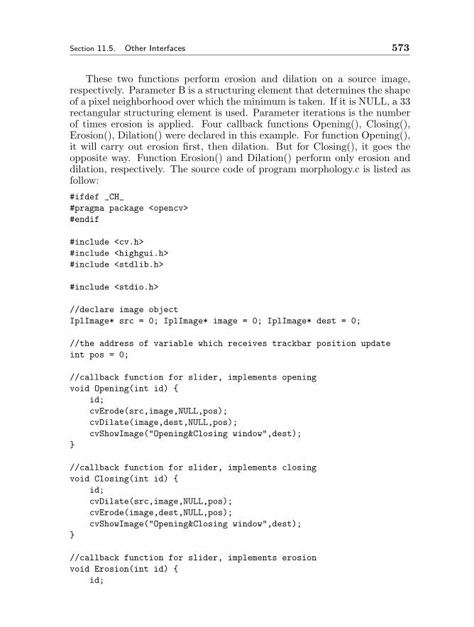
Section 11.5. Other Interfaces 573
These two functions perform erosion and dilation on a source image,respectively. Parameter B is a structuring element that determines the shapeof a pixel neighborhood over which the minimum is taken. If it is NULL, a 33rectangular structuring element is used. Parameter iterations is the numberof times erosion is applied. Four callback functions Opening(), Closing(),Erosion(), Dilation() were declared in this example. For function Opening(),it will carry out erosion first, then dilation. But for Closing(), it goes theopposite way. Function Erosion() and Dilation() perform only erosion anddilation, respectively. The source code of program morphology.c is listed asfollow:
#ifdef _CH_#pragma package <opencv>#endif
#include <cv.h>#include <highgui.h>#include <stdlib.h>
#include <stdio.h>
//declare image objectIplImage* src = 0; IplImage* image = 0; IplImage* dest = 0;
//the address of variable which receives trackbar position updateint pos = 0;
//callback function for slider, implements openingvoid Opening(int id)
id;cvErode(src,image,NULL,pos);cvDilate(image,dest,NULL,pos);cvShowImage("Opening&Closing window",dest);
//callback function for slider, implements closingvoid Closing(int id)
id;cvDilate(src,image,NULL,pos);cvErode(image,dest,NULL,pos);cvShowImage("Opening&Closing window",dest);
//callback function for slider, implements erosionvoid Erosion(int id)
id;
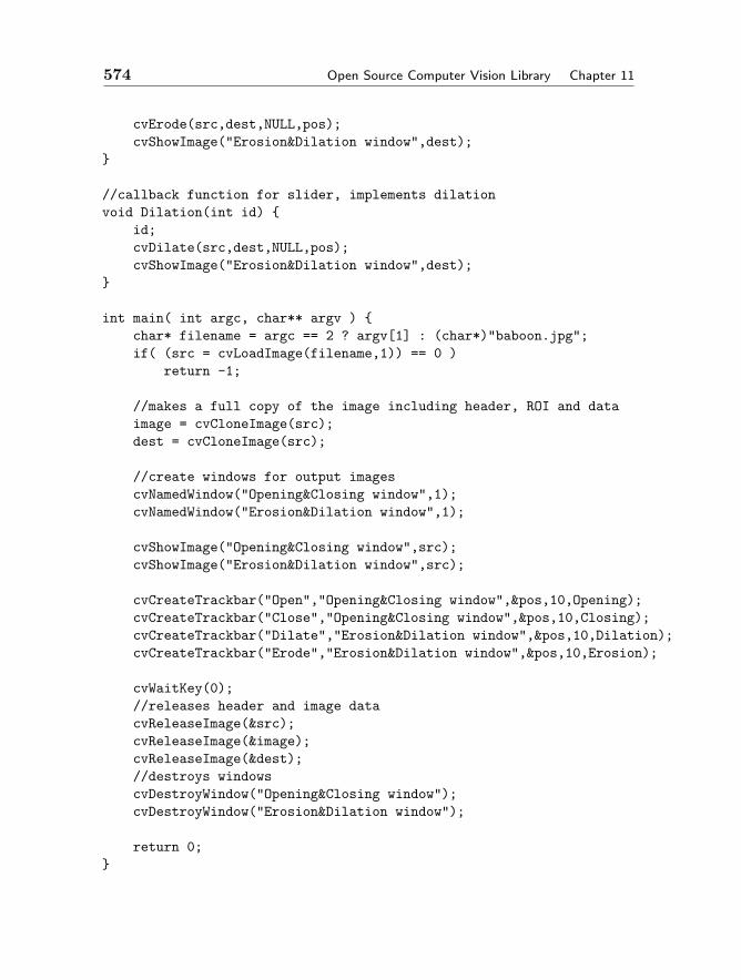
574 Open Source Computer Vision Library Chapter 11
cvErode(src,dest,NULL,pos);cvShowImage("Erosion&Dilation window",dest);
//callback function for slider, implements dilationvoid Dilation(int id)
id;cvDilate(src,dest,NULL,pos);cvShowImage("Erosion&Dilation window",dest);
int main( int argc, char** argv ) char* filename = argc == 2 ? argv[1] : (char*)"baboon.jpg";if( (src = cvLoadImage(filename,1)) == 0 )
return -1;
//makes a full copy of the image including header, ROI and dataimage = cvCloneImage(src);dest = cvCloneImage(src);
//create windows for output imagescvNamedWindow("Opening&Closing window",1);cvNamedWindow("Erosion&Dilation window",1);
cvShowImage("Opening&Closing window",src);cvShowImage("Erosion&Dilation window",src);
cvCreateTrackbar("Open","Opening&Closing window",&pos,10,Opening);cvCreateTrackbar("Close","Opening&Closing window",&pos,10,Closing);cvCreateTrackbar("Dilate","Erosion&Dilation window",&pos,10,Dilation);cvCreateTrackbar("Erode","Erosion&Dilation window",&pos,10,Erosion);
cvWaitKey(0);//releases header and image datacvReleaseImage(&src);cvReleaseImage(&image);cvReleaseImage(&dest);//destroys windowscvDestroyWindow("Opening&Closing window");cvDestroyWindow("Erosion&Dilation window");
return 0;
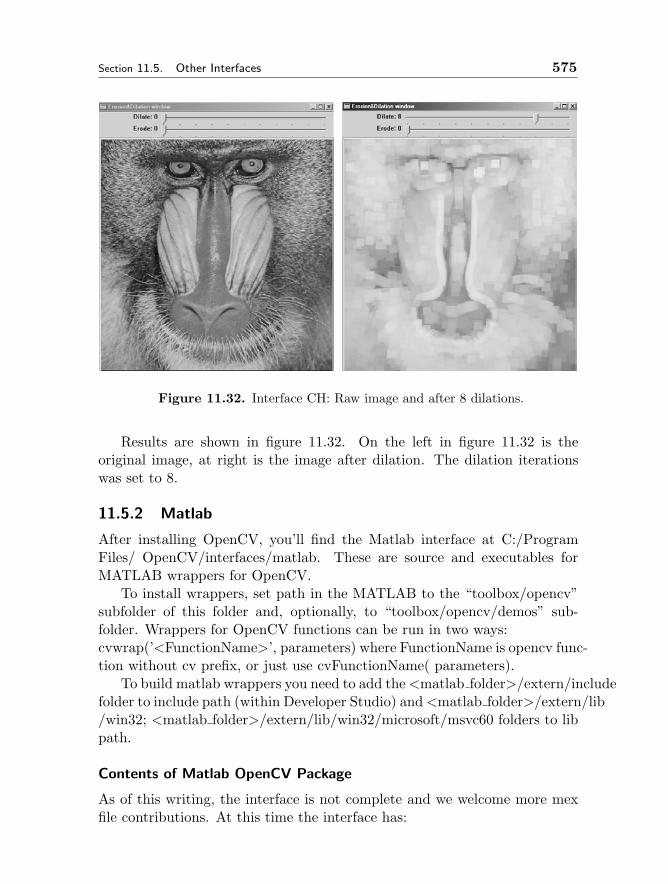
Section 11.5. Other Interfaces 575
Figure 11.32. Interface CH: Raw image and after 8 dilations.
Results are shown in figure 11.32. On the left in figure 11.32 is theoriginal image, at right is the image after dilation. The dilation iterationswas set to 8.
11.5.2 Matlab
After installing OpenCV, you’ll find the Matlab interface at C:/ProgramFiles/ OpenCV/interfaces/matlab. These are source and executables forMATLAB wrappers for OpenCV.
To install wrappers, set path in the MATLAB to the “toolbox/opencv”subfolder of this folder and, optionally, to “toolbox/opencv/demos” sub-folder. Wrappers for OpenCV functions can be run in two ways:cvwrap(’<FunctionName>’, parameters) where FunctionName is opencv func-tion without cv prefix, or just use cvFunctionName( parameters).
To build matlab wrappers you need to add the<matlab folder>/extern/includefolder to include path (within Developer Studio) and<matlab folder>/extern/lib/win32; <matlab folder>/extern/lib/win32/microsoft/msvc60 folders to libpath.
Contents of Matlab OpenCV Package
As of this writing, the interface is not complete and we welcome more mexfile contributions. At this time the interface has:
576 Open Source Computer Vision Library Chapter 11
cvadaptivethreshold.mcvapproxpoly.mcvcalcopticalflowpyrlk.mcvcanny.mcvcontourarea.mcvcontourboundingrect.mcvcontourperimeter.mcvdilate.mcvdisttransform.mcvdrawcontours.mcverode.mcvfindcontours.mcvfloodfill.mcvgoodfeaturestotrack.mcvlaplace.mcvmatchtemplate.mcvminmaxloc.mcvprecornerdetect.mcvpyrdown.mcvpyrup.mcvsobel.mcvthreshold.mcvupdatemotionhistory.mcvwrap.dll -- the mex wrapper
The demo directory contains:
’Canny Demo’, ’cannydemo’’Contour Demo’, ’contdemo’’Flood Fill Demo’, ’filldemo’’Optical Flow Demo’, ’flowdemo’
Programming example
Matlab is perhaps the tersest programming language. The code below runsthe Canny edge detector with (low,high) thresholds set to (120,200) withresulting input/output shown in figure 11.33.
I = imread(’Clone.jpg’); %Read in an imageC = cvcanny(I(:,:,2), 120,200,3); %Apply canny with thresholds (Low,High)
%(120,200), sobel size 3imshow(C); %Show the imageimwrite(C,’CloneCanny.bmp’,’bmp’); %Save image
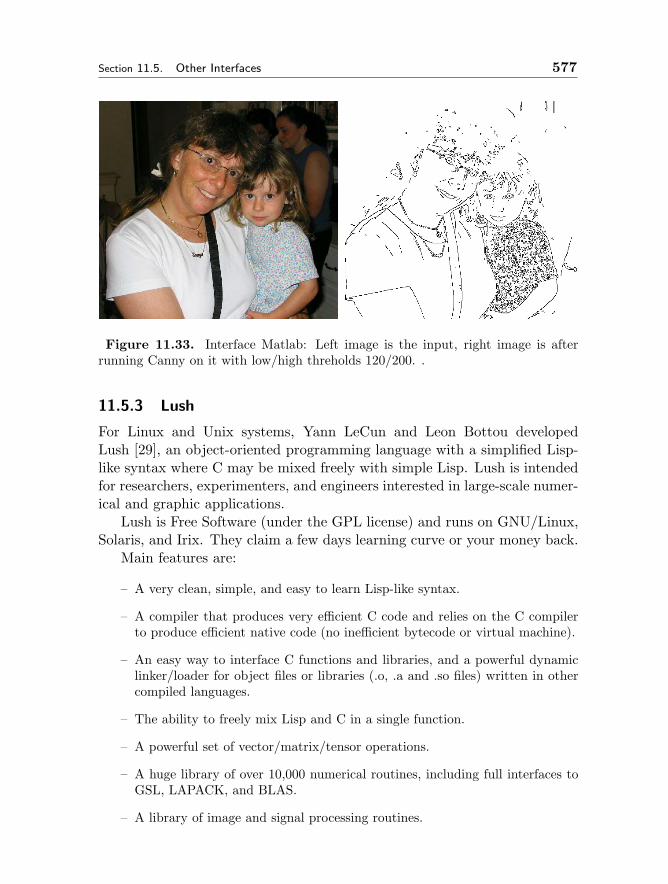
Section 11.5. Other Interfaces 577
Figure 11.33. Interface Matlab: Left image is the input, right image is afterrunning Canny on it with low/high threholds 120/200. .
11.5.3 Lush
For Linux and Unix systems, Yann LeCun and Leon Bottou developedLush [29], an object-oriented programming language with a simplified Lisp-like syntax where C may be mixed freely with simple Lisp. Lush is intendedfor researchers, experimenters, and engineers interested in large-scale numer-ical and graphic applications.
Lush is Free Software (under the GPL license) and runs on GNU/Linux,Solaris, and Irix. They claim a few days learning curve or your money back.
Main features are:
– A very clean, simple, and easy to learn Lisp-like syntax.
– A compiler that produces very efficient C code and relies on the C compilerto produce efficient native code (no inefficient bytecode or virtual machine).
– An easy way to interface C functions and libraries, and a powerful dynamiclinker/loader for object files or libraries (.o, .a and .so files) written in othercompiled languages.
– The ability to freely mix Lisp and C in a single function.
– A powerful set of vector/matrix/tensor operations.
– A huge library of over 10,000 numerical routines, including full interfaces toGSL, LAPACK, and BLAS.
– A library of image and signal processing routines.
578 Open Source Computer Vision Library Chapter 11
– An extensive set of graphic routines, including an object-oriented GUI toolkit,an interface to OpenGL/GLU/GLUT, and a soon-to-be-available interface tothe OpenInventor scene rendering engine.
– An interface to the Simple Directmedia Layer (SDL) multimedia library, in-cluding a sprite class with pixel-accurate collision detection.
– Sound and video grabbing (using ALSA and Video4Linux).
– Several libraries for machine learning, neural net, statistical estimation, Hid-den Markov Models (gblearning, Torch, HTK).
– libraries for computer vision (Intel Vision Library), and 3D scene rendering(OpenInventor, available soon).
– bindings to the JavaVM API and to the Python C API (available soon).
Lush is geared towards research and development in signal processing,image processing, machine learning, computer vision, bio-informatics, datamining, statistics, simulation, optimization, and artificial intelligence.
11.6 Appendix A
OpenCV has a “BSD” style license that basically allows royalty free com-mercial and research use subject to citation of the library. In particular, youmay use it in a for profit product without the need to open your product toothers. The license is as follows:
By downloading, copying, installing or using the software youagree to this license. If you do not agree to this license, do notdownload, install, copy or use the software.
Intel License AgreementFor Open Source Computer Vision Library
Copyright (C) 2000, 2001, Intel Corporation, all rights reserved.Third party copyrights are property of their respective owners.
Redistribution and use in source and binary forms, with or withoutmodification, are permitted provided that the following conditionsare met:
* Redistribution’s of source code must retain the above copyrightnotice, this list of conditions and the following disclaimer.
* Redistribution’s in binary form must reproduce the above

Section 11.7. Appendix B 579
copyright notice, this list of conditions and the followingdisclaimer in the documentation and/or other materials providedwith the distribution.
* The name of Intel Corporation may not be used to endorse orpromote products derived from this software without specificprior written permission.
This software is provided by the copyright holders andcontributors ‘‘as is’’ and any express or implied warranties,including, but not limited to, the implied warranties ofmerchantability and fitness for a particular purpose aredisclaimed. In no event shall the Intel Corporation orcontributors be liable for any direct, indirect, incidental,special, exemplary, or consequential damages (including, but notlimited to, procurement of substitute goods or services; loss ofuse, data, or profits; or business interruption) however causedand on any theory of liability, whether in contract, strictliability, or tort (including negligence or otherwise) arising inany way out of the use of this software, even if advised of thepossibility of such damage.
11.7 Appendix B
Partial “thank you” list for OpenCV:
Original OpenCV committee (vision, functionality proposals etc.):-----------------------------------------------------------------Dr. Gary Bradski, Vadim PisarevskyProf. Trevor DarrellProf. Irfan EssaProf. Jitendra MalikProf. Pietro PeronaProf. Stan SclaroffProf. Carlo Tomasi
People who helped to make OpenCV real (if you noticed some namesare missing, please mail to [email protected])----------------------------------------------------------------------------Name Company (time of Remarks
contribution/cooperation)
Alekseev, Aleksey Intel Corp. IppCV testingBoldyrev, Sergey Intel Corp. rpm spec, linux makefiles

580 Open Source Computer Vision Library Chapter 11
Breen, Ed ??? EiC intepreterDevernay, Frederic INRIA (?) cvcam patch (Linux version)Don Murray PointGrey PointGrey SDK and patches
for stereo gest. rec. codeDubey, Premnath ??? cvcam patch (Windows vers.)Halsall, Chris Open Source O-Reilly papers on OpenCV,
Solutions Inc. calibration app for Linuxpatches for Linux version
Khamenya, Valery BioVisioN AG OpenCV CVS repository atSourceForge
Rodyushkin, Konstantin Intel Corp. OpenCV to 3dFaceSchaefer, Dirk MD-Mathematische Original code for
Dienste GmbH Bayer->RGB pattern conv.Veretennikov, Eugene Intel Corp. Testing, comp. geo. functsWayne W. Cheng SoftIntegration Ch C/C++ intepreter, OpenCV
Ch toolbox (proposal + SDK)Muehlmann, Karsten Lehrstuhl fur Another stereo corresp.
Informatick V code (not included yet)Bouguet, Jean-Yves Intel Calibration and 3DNefian, Ara Intel eHMMDavies, Bob Intel Coding, test, user groupGrzeszczuk, Radek Intel Robust line fit
Active OpenCV forum participants (who helped us): Barbaresi,Abramo Betti, Gabriele Cao, Ning Cawkwell, Jack Chen, Gen-NanCheng, Michael Fritz, Frank Iannizotto, Giancarlo Lu, Le Kunz,Clay Ming, Li Philomin, Vasanth Zayed, Mohamed Rocha, JairoStewart, James Andr.
BUG reports:------------Small, Daniel;Carlos Andres Rocha;Shavit, Adi;Zivkovic, Zoranand other people from OpenCV forum at www.yahoogroups.com
Bibliography
[1] Open source computer vision library (opencv) main page. Available at:http://www.intel.com/research/mrl/research/opencv.
[2] Located at http://developer.intel.com/software/products/ipp/ippvm20/.[3] Intel performance libraries. Located at
http://developer.intel.com/software/products/perflib/.[4] Opencv user group. Located at: http://groups.yahoo.com/group/OpenCV/.

Bibliography 581
[5] Opencv course foilset. Located at: http://prdownloads.sourceforge.net/opencvlibrary/CVPR01 course.zip?download.
[6] Opencv download site. Located at: http://sourceforge.net/projects/opencvlibrary/.[7] G. Borgefors. Distance transformations in digital images. Computer Vision,
Graphics and Image Processing, pages 34, 344–371, 1986.[8] J.-Y. Bouguet. Pyramidal implementation of the lucas kanade feature tracker.
The paper is included into OpenCV distribution (algo tracking.pdf), 2000.[9] J.-Y. Bouguet and P. Perona. Camera Calibration from Points and Lines in
Dual-Space Geometry. Technical report, California Institute of Technology,1998.
[10] J.-Y. Bouguet and P. Perona. Camera calibration from points and lines in thereciprocal space. Submitted to European Conference on Computer Vision, 1998.
[11] G. Bradski. Computer vision face tracking as a component of a perceptual userinterface. IEEE WACV’98, included into OpenCV distribution (camshift.pdf),1998.
[12] G. Bradski, J-Y. Bouguet, and V. Pisarevsky. Computer vision recipes withopencv (working title). Springer. In Press, Winter 2003.
[13] G. Bradski and J. Davis. Motion segmentation and pose recognition with mo-tion history gradients. IEEE WACV’00, pages 214–219, 2000.
[14] G. Bradski. The opencv library. Dr. Dobb’s Journal, pages 120–125, 2000.[15] H.H. Cheng. The ch language environment user’s guide. SoftIntegration, Inc.
In http://www.softintegration.com, 2002.[16] H.H. Cheng. Scientific computing in the ch programming language. Scientific
Programming, Vol. 2, No 3, pages 49–75, Fall, 1993.[17] J. Davis and Bobick. The representation and recognition of action using tem-
poral templates. MIT Media Lab Technical Report, page 402, 1997.[18] D.F. DeMenthon and L.S. Davis. Model-based object pose in 25 lines of code.
In Proceedings of ECCV ’92, pages pp. 335–343, 1992.[19] A. Elgammal, D. Harwood, and L. Davis. Non-parametric model for background
subtraction. 6th European Conference of Computer Vision, 2000.[20] S. M. Ettinger, M. C. Nechyba, P. G. Ifju, and M. Waszak. Vision-guided
flight stability and control for micro air vehicles. Proc. IEEE Int. Conferenceon Intelligent Robots and Systems see http://www.mil.ufl.edu/ nechyba/mav/,2002.
[21] Heikkila and Silven. A four-step camera calibration procedure with implicitimage correction. CVPR97, 1997.
[22] B.K.P. Horn and B.G. Schunck. Determining optical flow. Artificial Intelligence,pages 17, pp. 185–203, 1981.
[23] M. Hu. Visual pattern recognition by moment invariants. IRE Transactions onInformation Theory, pages 8:2, pp. 179–187, 1962.
[24] J. Iivarinen, M. Peura, J. Srel, and A. Visa. Compari-son of combined shape descriptors for irregular objects. 8thBritish Machine Vision Conference, BMVC’97, online version athttp://www.cis.hut.fi/research/IA/paper/publications/bmvc97/bmvc97.html,1997.
582 Open Source Computer Vision Library Chapter 11
[25] SoftIntegration Inc. The ch language environment sdk user’s guide.http://www.softintegration.com, 2002.
[26] J. Matas, C. Galambos, and J. Kittler. Progressive probabilistic hough trans-form. British Machine Vision Conference, 1998.
[27] M. Kass, A. Witkin, and D. Terzopoulos. Snakes: Active contour models.International Journal of Computer Vision, pages pp. 321–331, 1988.
[28] A. Kuranov, R. Lienhart, and V. Pisarevsky. An empirical analysis of boostingalgorithms for rapid objects with an extended set of haar-like features. TechnicalReport MRL-TR-July02-01, Intel Corporation, 2002.
[29] Y. LeCun and L. Bottou. Lush programing language.http://lush.sourceforge.net/index.html, 2002.
[30] B. Lucas and T. Kanade. An iterative image registration technique with anapplication to stereo vision. Proc. of 7th International Joint Conference onArtificial Intelligence (IJCAI), pages 674–679, 1981.
[31] A. Nefian and M. Hayes. Hidden markov models for face recognition.[32] Y. Rubner and C. Tomasi. Texture metrics. Proceeding of the IEEE Interna-
tional Conference on Systems, Man, and Cybernetics, San-Diego, CA, pagespp. 4601–4607, October 1998.
[33] Y. Rubner, C. Tomasi, and L.J. Guibas. Metrics for distributions with ap-plications to image databases. Proceedings of the 1998 IEEE InternationalConference on Computer Vision, Bombay, India, pages pp. 59–66, January1998.
[34] Y. Rubner, C. Tomasi, and L.J. Guibas. The earth mover’s distance as ametric for image retrieval. Technical Report STAN-CS-TN-98-86, Departmentof Computer Science, Stanford University, September 1998.
[35] B. Schiele and J.L. Crowley. Object recognition using multidimensional recep-tive field histograms. In ECCV (1), pages 610–619, 1996.
[36] B. Schiele and J.L. Crowley. Recognition without correspondence using multi-dimensional receptive field histograms. In International Journal of ComputerVision, pages 36 (1), pp. 31–50, January 2000.
[37] J. Serra. Image analysis and mathematical morphology. Academic Press, 1982.[38] M. J. Swain and D. H. Ballard. Color indexing. International Journal of
Computer Vision, Vol. 7, No. 1, pages 11–32, 1991.[39] K. Toyama, J. Krumm, B. Brumitt, and B. Meyers. Wallflower: Principles and
practice of background maintenance. ICCV’99, 1999.[40] P. Viola and M. Jones. Robust real-time object detection. International Journal
of Computer Vision, 2002.[41] G. Welch and G. Bishop. An introduction to the kalman filter. Technical Re-
port TR95-041, University of North Carolina at Chapel Hill. Online version isavailable at http://www.cs.unc.edu/˜welch/kalman/kalman filter/kalman.html,1995.
[42] C. Wren, A. Azarbayejani, T. Darrell, and A. Pentland. Pfinder: Real-time tracking of the human body. Technical Report 353, MIT Media Lab-oratory Perceptual Computing Section Technical Report, 1997, available at:http://pfinder.www.media.mit.edu/projects/pfinder/.

Bibliography 583
[43] Z. Zhang. Parameter estimation techniques: A tutorial with application toconic fitting. Image and Vision Computing Journal, 1996.
[44] Z. Zhang. A flexible new technique for camera calibration. IEEE Transactionson Pattern Analysis and Machine Intelligence, pages 22(11):1330–1334, 2000.
[45] Z. Zhang. Flexible camera calibration by viewing a plane from unknown ori-entations. International Conference on Computer Vision (ICCV’99), Corfu,Greece, pages 666–673, September 1999.

Chapter 12
SOFTWARE ARCHITECTUREFOR COMPUTER VISION
Alexandre R.J. Francois
12.1 INTRODUCTION
This chapter highlights and addresses architecture level software develop-ment issues facing researchers and practitioners in the field of ComputerVision. A new framework, or architectural style, called SAI, is introduced.It provides a formalism for the design, implementation and analysis of soft-ware systems that perform distributed parallel processing of generic datastreams. The SAI style is illustrated with a number of Computer Visionrelated examples. A code-level tutorial provides a hands-on introduction tothe development of image stream manipulation applications using MFSM,an open source architectural middleware implementing the SAI style.
12.1.1 Motivation
The emergence of comprehensive code libraries in a research field is a signthat researchers and practitioners are seriously considering and addressingsoftware engineering and development issues. In this sense, the introductionof the Intel OpenCV library [2] certainly represents an important milestonefor Computer Vision. The motivation behind building and maintaining codelibraries is to address reusability and efficiency, by providing a set of “stan-dard” data structures and implementations of classic algorithms. In a fieldlike Computer Vision, with a rich theoretical history, implementation issuesare often regarded as secondary to the pure research components outside
585
586 Software Architecture for Computer Vision Chapter 12
of specialty subfields, such as Real-Time Computer Vision (see e.g. [27]).Nevertheless, beyond reducing development and debugging time, good codedesign and reusability are key to such fundamental principles of scientificresearch as experiment reproducibility and objective comparison with theexisting state of the art.
For example, these issues are apparent in the subfield of video process-ing/analysis, which, due to the conjunction of technical advances in variousenabling hardware performance (including processors, cameras and storagemedia) and high priority application domains(e.g. visual surveillance [3]),has recently become a major area of research. One of the most spectacularside effects of this activity is the amount of test data generated, an impor-tant part of which is made public. The field has become so rich in analysistechniques that any new method must almost imperatively be compared tothe state-of the art in its class to be seriously considered by the community.Reference data sets, complete with ground truth data, have been producedand compiled for this very purpose (see e.g. [6, 7, 8, 9]). Similarly, a reli-able, reusable and consistent body of code for established–and “challenger”–algorithms could certainly facilitate the performance comparison task. Someeffort is made toward developing open platforms for evaluation (see e.g. [19]).Such properties as modularity contribute to code reuse, and fair and consis-tent testing and comparison. However, building a platform generic enough tonot only accommodate current methods, but also allow to incorporate otherrelevant algorithms, some of them not yet developed, is a major challenge.It is well known in the software industry that introducing features that werenot planned for at design time in a software system is a least an extremelyhard problem, and generally a recipe for disaster. Software Engineering isthe field of study devoted to addressing these and other issues of softwaredevelopment in industrial settings. The parameters and constraints of indus-trial software development are certainly very different of that encountered ina research environment, and thus Software Engineering techniques are oftenunadapted to the latter.
In a research environment, software is developed to demonstrate the va-lidity and evaluate the performance of an algorithm. The main performanceaspect on which algorithms are evaluated is of course the accuracy of theiroutput. Another aspect of performance is measured in terms of systemthroughput, or algorithm execution time. This aspect is all the more rel-evant as the amount of data to be processed increases, leaving less and lesstime for storing and off-line processing. The metrics used for this type of per-formance assessment are often partial. In particular, theoretical complexityanalysis is but a prediction tool, which cannot account for the many other

Section 12.1. Introduction 587
factors involved in a particular system’s performance. Many algorithms areclaimed to be “real-time.” Some run at a few frames per second, but “couldbe implemented to run in real-time,” or simply will run faster on the nextgeneration machines (or the next...). Others have been the object of care-ful design and specialization to allow a high processing rate on constrainedequipment. The general belief that increasing computing power can makeany system (hardware and software) run faster relies on the hidden or im-plied assumption of system scalability, a property that cannot and shouldnot be taken for granted. Indeed, the performance of any given algorithmimplementation is highly dependent on the overall software system in whichit is operated (see e.g. [20]). Video analysis applications commonly involveimage input (from file or camera) and output (to file or display) code, theperformance of which can greatly impact the perceived performance of theoverall application, and in some cases the performance of the individual al-gorithms involved in the processing. Ideally, if an algorithm or technique isrelevant for a given purpose, it should be used in its best available imple-mentation, on the best available platform, with the opportunity of upgradingeither when possible.
As Computer Vision is maturing as a field, and finds new applicationsin a variety of domains, the issue of interoperability becomes central to itssuccessful integration as an enabling technology in cross-disciplinary efforts.Technology transfer from research to industry could also be facilitated bythe adoption of relevant methodologies in the development of research code.
If these aspects are somewhat touched in the design of software libraries,a consistent, generic approach requires a higher level of abstraction. Thisis the realm of Software Architecture, the field of study concerned with thedesign, analysis and implementation of software systems. Shaw and Garlangive the following definition in [26]:
“As the size and complexity of software systems increase, the de-sign and specification of overall system structure become moresignificant issues than the choice of algorithms and data struc-tures of computation. Structural issues include the organiza-tion of a system as a composition of components; global controlstructures; the protocols for communication, synchronization anddata access; the assignment of functionality to design elements;the composition of design elements; physical distribution; scalingand performance; dimensions of evolution; and selection amongdesign alternatives. This is the Software Architecture level ofdesign.”
588 Software Architecture for Computer Vision Chapter 12
They also provide the framework for architecture description and anal-ysis used in the remainder of this chapter. A specific architecture can bedescribed as a set of computational components, and a their inter-relations,or connectors. An architectural style characterizes families of architecturesthat share some patterns of structural organization. Formally, an architec-tural style defines a vocabulary of components and connector types, and aset of constraints on how instances of these types can be combined to forma valid architecture.
If Software Architecture is a relatively young field, software architectureshave been developed since the first software was designed. Classic styleshave been identified and studied informally and formally, their strengths andshortcomings analyzed. A major challenge for the software architect is thechoice of an appropriate style when designing a given system, as an architec-tural style may be ideal for some applications, while unadapted for others.The goal here is to help answer this question by providing the ComputerVision community with a flexible and generic architectural model. The firststep toward the choice–or the design–of an architectural style is the identi-fication and formulation of the core requirements for the target system(s).An appropriate style should support the design and implementation of soft-ware systems capable of handling images, 2-D and 3-D geometric models,video streams, various data structures, in a variety of algorithms and com-putational frameworks. These applications may be interactive and/or havereal-time constraints. Going beyond pure Computer Vision systems, pro-cessing of other data types, such as sound and haptics data, should alsobe supported, in a consistent manner, in order to compose large scale inte-grated systems, such as immersive simulations. Note that interaction has avery particular status in this context, as data originating from the user canbe both an input to an interactive Computer Vision system, and the outputof a vision-based perceptual interface subsystem.
This set of requirements can be captured under the general definition ofcross-disciplinary dynamic systems, possibly involving real-time constraints,user immersion and interaction. A fundamental underlying computationalinvariant across such systems is distributed parallel processing of generic data-streams. As no existing architectural model could entirely and satisfactorilyaccount for such systems, a new model was introduced.
12.1.2 Contribution
SAI (Software Architecture for Immersipresence) is a new software architec-ture model for designing, analyzing and implementing applications perform-
Section 12.1. Introduction 589
ing distributed, asynchronous parallel processing of generic data streams.The goal of SAI is to provide a universal framework for the distributed im-plementation of algorithms and their easy integration into complex systemsthat exhibit desirable software engineering qualities such as efficiency, scala-bility, extensibility, reusability and interoperability. SAI specifies a new ar-chitectural style (components, connectors and constraints). The underlyingextensible data model and hybrid (shared repository and message-passing)distributed asynchronous parallel processing model allow natural and effi-cient manipulation of generic data streams, using existing libraries or nativecode alike. The modularity of the style facilitates distributed code devel-opment, testing, and reuse, as well as fast system design and integration,maintenance and evolution. A graph-based notation for architectural de-signs allows intuitive system representation at the conceptual and logicallevels, while at the same time mapping closely to processes.
MFSM (Modular Flow Scheduling Middleware) [12] is an architecturalmiddleware implementing the SAI style. Its core element, the FSF library, isa set of extensible classes that can be specialized to define new data structuresand processes, or encapsulate existing ones (e.g. from libraries). MFSM is anopen source project, released under the GNU Lesser General Public License[1]. A number of software modules regroup specializations implementingspecific algorithms or functionalities. They constitute a constantly growingbase of open source, reusable code, maintained as part of the MFSM project.The project also includes extensive documentation, including user guide,reference guide and tutorials.
12.1.3 Outline
This chapter is a hands on introduction to the design of Computer Visionapplications using SAI, and their implementation using MFSM.
Section 12.2 is an introduction to SAI. Architectural principles for dis-tributed parallel processing of generic data streams are first introduced, incontrast to the classic Pipes and Filters model. These principles are thenformulated into a new architectural style. A graph-based notation for archi-tectural designs is introduced. Architectural patterns are illustrated througha number of demonstration projects ranging from single stream automaticreal-time video processing to fully integrated distributed interactive systemsmixing live video, graphics and sound. A review of key architectural prop-erties of SAI concludes the section.
Section 12.3 is an example-based, code-level tutorial on writing imagesstream processing applications with MFSM. It begins with a brief overview
590 Software Architecture for Computer Vision Chapter 12
of the MFSM project and its implementation of SAI. Design and implemen-tation of applications for image stream manipulation is then explained indetail using simple examples, based on those used in the online MFSM userguide. The development of specialized SAI components is also addressed atthe code level. In particular, the implementation of a generic image datastructure (object of an open source module) and its use in conjunction withthe OpenCV library in specialized processes are described step by step.
In conclusion, Section 12.4 offers a summary of the chapter and someperspectives on future directions for SAI and MFSM.
12.2 SAI: A SOFTWARE ARCHITECTURE MODEL
This section is an introduction to the SAI architectural model for distributedparallel processing of generic data streams.
The most common architectural styles for data stream processing ap-plications are derived from the classic Pipes and Filters model. It is, forexample, the underlying model of the Microsoft DirectShow library, partof the DirectX suite [24]. After a brief review of the Pipes and Filters ar-chitectural style, of its strengths and weaknesses, a new hybrid model isintroduced, that addresses the identified limitations while preserving thedesirable properties. This new model is formally defined as the SAI ar-chitectural style. Its component and connector types are defined, togetherwith the corresponding constraints on instances interaction. The underlyingdata and processing models are explicited and analyzed. Simultaneously,graphical symbols are introduced to represent each element type. Togetherthese symbols constitute a graph-based notation system for representing ar-chitectural designs. Architectural patterns are illustrated with a numberof demonstration projects ranging from single stream automatic real-timevideo processing to fully integrated distributed interactive systems mixinglive video, graphics and sound. Finally, relevant architectural properties ofthis new style are summarized.
12.2.1 Beyond Pipes and Filters
The Pipes and Filters model is an established (and popular) model for datastream manipulation and processing architectures. In particular, it is a clas-sic model in the domains of signal processing, parallel processing and dis-tributed processing [10], to name but a few. This section first offers anoverview of the classic Pipes and Filters architectural style, emphasizing itsdesirable properties, and highlighting its main limitations. A hybrid modelis then outlined, that aims at addressing the limitations while preserving the
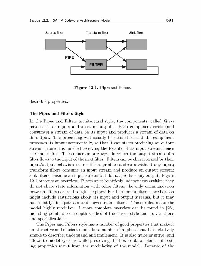
Section 12.2. SAI: A Software Architecture Model 591
Source filter Sink filterTransform filter
FILTER
PIPE
Figure 12.1. Pipes and Filters.
desirable properties.
The Pipes and Filters Style
In the Pipes and Filters architectural style, the components, called filtershave a set of inputs and a set of outputs. Each component reads (andconsumes) a stream of data on its input and produces a stream of data onits output. The processing will usually be defined so that the componentprocesses its input incrementally, so that it can starts producing an outputstream before it is finished receiving the totality of its input stream, hencethe name filter. The connectors are pipes in which the output stream of afilter flows to the input of the next filter. Filters can be characterized by theirinput/output behavior: source filters produce a stream without any input;transform filters consume an input stream and produce an output stream;sink filters consume an input stream but do not produce any output. Figure12.1 presents an overview. Filters must be strictly independent entities: theydo not share state information with other filters, the only communicationbetween filters occurs through the pipes. Furthermore, a filter’s specificationmight include restrictions about its input and output streams, but it maynot identify its upstream and downstream filters. These rules make themodel highly modular. A more complete overview can be found in [26],including pointers to in-depth studies of the classic style and its variationsand specializations.
The Pipes and Filters style has a number of good properties that make itan attractive and efficient model for a number of applications. It is relativelysimple to describe, understand and implement. It is also quite intuitive, andallows to model systems while preserving the flow of data. Some interest-ing properties result from the modularity of the model. Because of the
592 Software Architecture for Computer Vision Chapter 12
well-defined and constrained interaction modalities between filters, complexsystems described in terms of data streams flowing from filter to filter areeasily understandable as a series of well defined local transformations. Theimplementation details of each filter are irrelevant to the high level under-standing of the overall system, as long as a logical definition of their behavioris specified (input, transformation and output). The localization and isola-tion of computations facilitates system design, implementation, maintenanceand evolution. Reversely, filters can be implemented and tested separately.Furthermore, because filters are independent, the model naturally supportsparallel and distributed processing.
These properties of the model provide an answer to some of the soft-ware issues highlighted in the introduction. Because of their independence,filters certainly allow reusability and interoperability. Parallelism and dis-tributability, to a certain extent, should contribute to efficiency and scalabil-ity. It would seem that it is a perfect model for real-time, distributed parallelprocessing of data streams. However, a few key shortcomings and limitationsmake it unsuitable for designing cross-disciplinary dynamic systems, possiblyinvolving real-time constraints, user immersion and interaction.
The first set of limitations is related to efficiency. If the pipes are first-in-first-out buffers, as suggested by the model, the overall throughput of aPipes and Filters system is imposed by the transmission rate of the slowestfilter in the system. If filters independence provide a natural design for paral-lel (and/or distributed) processing, the pipes impose arbitrary transmissionbottlenecks that make the model non optimal. Figure 12.2 illustrates inef-ficiency limitations inherent to the distribution and transmission of data inPipes and Filters models. Each filter’s output data must be copied to itsdownstream filter(s)’ input, which can lead to massive and expensive datacopying. Furthermore, the model does not provide any consistent mecha-nism to maintain correspondences between separate but related streams (e.g.when the results of different process paths must be combined to produce acomposite output). Such stream synchronization operations require datacollection from different repositories, possibly throughout the whole system,raising not only search-related efficiency issues, but also dependency-drivendistributed buffer maintenance issues. These can only be solved at the priceof breaking the strict filter independence rule, e.g. by the introduction of ahigher level system manager.
The second set of limitations is related to the simplicity of the model. Asthey are not part of the data streams, process parameters (state data storedin the filters) are not modeled consistently with process data (input datastreams). As a result, the pure Pipes and Filters model is ill-suited for de-
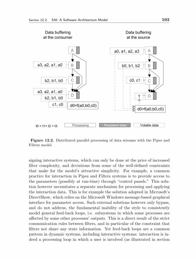
Section 12.2. SAI: A Software Architecture Model 593
Persistent data
a0, a1, a2, a3 A
B
C
D
b0, b1, b2
c0, c1
?
a0, a1, a2, a3
b0, b1, b2
c0, c1
?
d0=f(a0,b0,c0)
A
B
C
D
c1, c0 d0=f(a0,b0,c0)
a3, a2, a1, a0
b2, b1, b0
b2, b1, b0
a3, a2, a1, a0
c1, c0
a3, a2, a1, a0
b2, b1, b0
b2, b1, b0
a3, a2, a1, a0
Processing Volatile dataProcessing Volatile datat0 < t1< t2 < t3
Data bufferingat the source
Data bufferingat the consumer
Figure 12.2. Distributed parallel processing of data streams with the Pipes andFilters model.
signing interactive systems, which can only be done at the price of increasedfilter complexity, and deviations from some of the well-defined constraintsthat make for the model’s attractive simplicity. For example, a commonpractice for interaction in Pipes and Filters systems is to provide access tothe parameters (possibly at run-time) through “control panels.” This solu-tion however necessitates a separate mechanism for processing and applyingthe interaction data. This is for example the solution adopted in Microsoft’sDirectShow, which relies on the Microsoft Windows message-based graphicalinterface for parameter access. Such external solutions however only bypass,and do not address, the fundamental inability of the style to consistentlymodel general feed-back loops, i.e. subsystems in which some processes areaffected by some other processes’ outputs. This is a direct result of the strictcommunication rules between filters, and in particular of the constraint thatfilters not share any state information. Yet feed-back loops are a commonpattern in dynamic systems, including interactive systems: interaction is in-deed a processing loop in which a user is involved (as illustrated in section
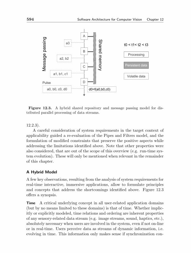
594 Software Architecture for Computer Vision Chapter 12
A
B
C
D
a0, b0, c0, d0
a3
a2, b2
a1, b1, c1
Pulse
Volatile data
t0 < t1< t2 < t3M
essa
ge p
assi
ng
Persistent data
Processing
Shared m
emory
d0=f(a0,b0,c0)
Figure 12.3. A hybrid shared repository and message passing model for dis-tributed parallel processing of data streams.
12.2.3).A careful consideration of system requirements in the target context of
applicability guided a re-evaluation of the Pipes and Filters model, and theformulation of modified constraints that preserve the positive aspects whileaddressing the limitations identified above. Note that other properties werealso considered, that are out of the scope of this overview (e.g. run-time sys-tem evolution). These will only be mentioned when relevant in the remainderof this chapter.
A Hybrid Model
A few key observations, resulting from the analysis of system requirements forreal-time interactive, immersive applications, allow to formulate principlesand concepts that address the shortcomings identified above. Figure 12.3offers a synopsis.
Time A critical underlying concept in all user-related application domains(but by no means limited to these domains) is that of time. Whether implic-itly or explicitly modeled, time relations and ordering are inherent propertiesof any sensory-related data stream (e.g. image streams, sound, haptics, etc.),absolutely necessary when users are involved in the system, even if not on-lineor in real-time. Users perceive data as streams of dynamic information, i.e.evolving in time. This information only makes sense if synchronization con-
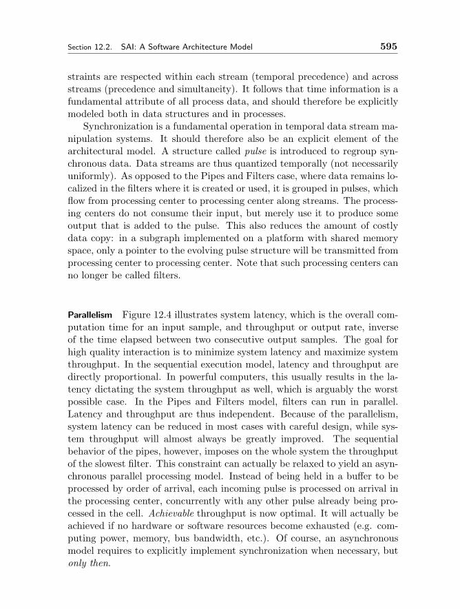
Section 12.2. SAI: A Software Architecture Model 595
straints are respected within each stream (temporal precedence) and acrossstreams (precedence and simultaneity). It follows that time information is afundamental attribute of all process data, and should therefore be explicitlymodeled both in data structures and in processes.
Synchronization is a fundamental operation in temporal data stream ma-nipulation systems. It should therefore also be an explicit element of thearchitectural model. A structure called pulse is introduced to regroup syn-chronous data. Data streams are thus quantized temporally (not necessarilyuniformly). As opposed to the Pipes and Filters case, where data remains lo-calized in the filters where it is created or used, it is grouped in pulses, whichflow from processing center to processing center along streams. The process-ing centers do not consume their input, but merely use it to produce someoutput that is added to the pulse. This also reduces the amount of costlydata copy: in a subgraph implemented on a platform with shared memoryspace, only a pointer to the evolving pulse structure will be transmitted fromprocessing center to processing center. Note that such processing centers canno longer be called filters.
Parallelism Figure 12.4 illustrates system latency, which is the overall com-putation time for an input sample, and throughput or output rate, inverseof the time elapsed between two consecutive output samples. The goal forhigh quality interaction is to minimize system latency and maximize systemthroughput. In the sequential execution model, latency and throughput aredirectly proportional. In powerful computers, this usually results in the la-tency dictating the system throughput as well, which is arguably the worstpossible case. In the Pipes and Filters model, filters can run in parallel.Latency and throughput are thus independent. Because of the parallelism,system latency can be reduced in most cases with careful design, while sys-tem throughput will almost always be greatly improved. The sequentialbehavior of the pipes, however, imposes on the whole system the throughputof the slowest filter. This constraint can actually be relaxed to yield an asyn-chronous parallel processing model. Instead of being held in a buffer to beprocessed by order of arrival, each incoming pulse is processed on arrival inthe processing center, concurrently with any other pulse already being pro-cessed in the cell. Achievable throughput is now optimal. It will actually beachieved if no hardware or software resources become exhausted (e.g. com-puting power, memory, bus bandwidth, etc.). Of course, an asynchronousmodel requires to explicitly implement synchronization when necessary, butonly then.
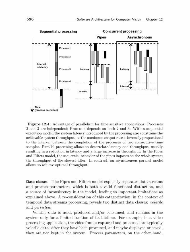
596 Software Architecture for Computer Vision Chapter 12
Time(process execution)
Sequential processing
Pipes Asynchronous
Interval= latency
Latency
Interval
Process 1
Process 2
Process 3
Process 4
Latency
Interval
Concurrent processing
Figure 12.4. Advantage of parallelism for time sensitive applications. Processes2 and 3 are independent; Process 4 depends on both 2 and 3. With a sequentialexecution model, the system latency introduced by the processing also constrains theachievable system throughput, as the maximum output rate is inversely proportionalto the interval between the completion of the processes of two consecutive timesamples. Parallel processing allows to decorrelate latency and throughput, usuallyresulting in a reduction in latency and a large increase in throughput. In the Pipesand Filters model, the sequential behavior of the pipes imposes on the whole systemthe throughput of the slowest filter. In contrast, an asynchronous parallel modelallows to achieve optimal throughput.
Data classes The Pipes and Filters model explicitly separates data streamsand process parameters, which is both a valid functional distinction, anda source of inconsistency in the model, leading to important limitations asexplained above. A re-consideration of this categorization, in the context oftemporal data streams processing, reveals two distinct data classes: volatileand persistent.
Volatile data is used, produced and/or consumed, and remains in thesystem only for a limited fraction of its lifetime. For example, in a videoprocessing application, the video frames captured and processed are typicallyvolatile data: after they have been processed, and maybe displayed or saved,they are not kept in the system. Process parameters, on the other hand,
Section 12.2. SAI: A Software Architecture Model 597
must remain in the system for the whole duration of its activity. Note thattheir value can change in time. They are dynamic yet persistent data.
All data, volatile or persistent, should be encapsulated in pulses. Pulsesholding volatile data flow down streams defined by connections between theprocessing centers, in a message passing fashion. They trigger computations,and are thus called active pulses. In contrast, pulses holding persistent in-formation are held in repositories, where the processing centers can accessthem in a concurrent shared memory access fashion. This hybrid modelcombining message passing and shared repository communication, combinedwith a unified data model, provides a universal processing framework. Inparticular, feed-back loops can now be explicitly and consistently modeled.
From the few principles and concepts outlined above emerged a newarchitectural style. Because of the context of its development, the new stylewas baptized SAI, for “Software Architecture for Immersipresence.”
12.2.2 The SAI Architectural Style
This section offers a more formal definition of the SAI architectural style.Graphical symbols are introduced to represent each element type. Togetherthese symbols constitute a graph-based notation system for representing ar-chitectural designs. In addition, when available, the following color codingwill be used: green for processing, red for persistent data, blue for volatiledata. Figure 12.5 presents a summary of the proposed notation.
In the remainder of this chapter, the distinction between an object typeand an instance of the type will be made explicitly only when required bythe context.
Components and connectors
The SAI style defines two types of components: cells and sources. Cells areprocessing centers. They do not store any state data related to their compu-tations. The cells constitute an extensible set of specialized components thatimplement specific algorithms. Each specialized cell type is identified by atype name (string), and is logically defined by its input data, its parametersand its output. Cell instances are represented graphically as green squares.A cell can be active or inactive, in which case it is transparent to the system.Sources are shared repository of persistent data. Source instances are repre-sented as red disks or circles. Two types of connectors link cells to cells andcells to sources. Cell to source connectors give the cell access to the sourcedata. Cell to cell connectors define data conduits for the streams. The se-mantics of these connectors are relaxed compared to that of pipes (which
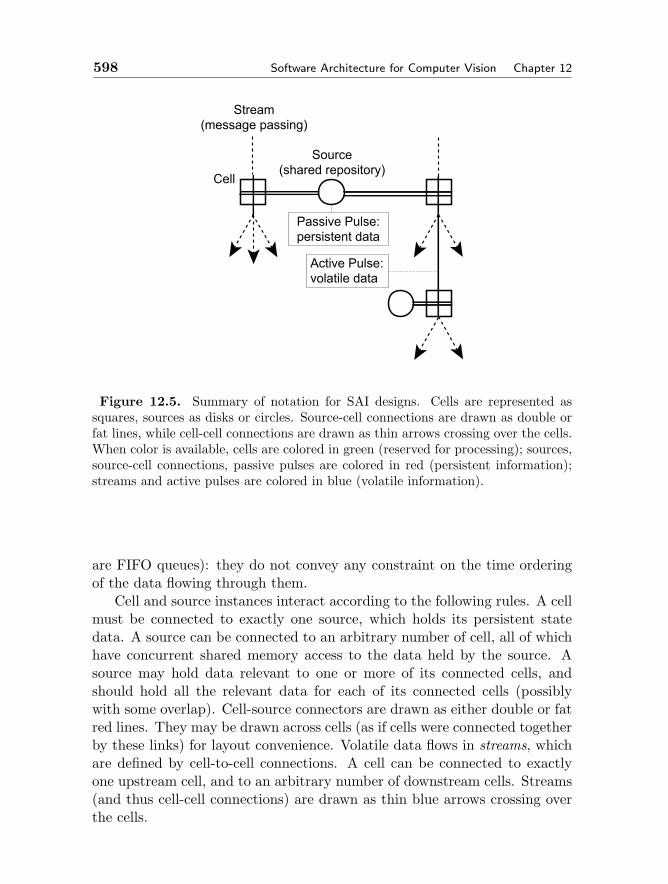
598 Software Architecture for Computer Vision Chapter 12
Cell
Passive Pulse:persistent data
Stream(message passing)
Active Pulse:volatile data
Source(shared repository)
Figure 12.5. Summary of notation for SAI designs. Cells are represented assquares, sources as disks or circles. Source-cell connections are drawn as double orfat lines, while cell-cell connections are drawn as thin arrows crossing over the cells.When color is available, cells are colored in green (reserved for processing); sources,source-cell connections, passive pulses are colored in red (persistent information);streams and active pulses are colored in blue (volatile information).
are FIFO queues): they do not convey any constraint on the time orderingof the data flowing through them.
Cell and source instances interact according to the following rules. A cellmust be connected to exactly one source, which holds its persistent statedata. A source can be connected to an arbitrary number of cell, all of whichhave concurrent shared memory access to the data held by the source. Asource may hold data relevant to one or more of its connected cells, andshould hold all the relevant data for each of its connected cells (possiblywith some overlap). Cell-source connectors are drawn as either double or fatred lines. They may be drawn across cells (as if cells were connected togetherby these links) for layout convenience. Volatile data flows in streams, whichare defined by cell-to-cell connections. A cell can be connected to exactlyone upstream cell, and to an arbitrary number of downstream cells. Streams(and thus cell-cell connections) are drawn as thin blue arrows crossing overthe cells.
Section 12.2. SAI: A Software Architecture Model 599
Data model
Data, whether persistent or volatile, is held in pulses. A pulse is a carrier forall the synchronous data corresponding to a given time stamp in a stream.Information in a pulse is organized as a mono-rooted composition hierarchyof node objects. The nodes constitute an extensible set of atomic data unitsthat implement or encapsulate specific data structures. Each specializednode type is identified by a type name (string). Node instances are identifiedby a name. The notation adopted to represent node instances and hierarchiesof node instances makes use of nested parentheses, e.g.: (NODE TYPE ID“Node name” (...) ... ). This notation may be used to specify a cell’s output,and for logical specification of active and passive pulses.
Each source contains a passive pulse, which encodes the instantaneousstate of the data structures held by the source. Volatile data flows in streams,that are temporally quantized into active pulses. Pulses are representedgraphically as a root (solid small disk) and a hierarchy of nodes (small cir-cles); passive pulses may be rooted in the circle or disk representing thesource.
Processing model
When an active pulse reaches a cell, it triggers a series of operations thatcan lead to its processing by the cell (hence the “active” qualifier). Pro-cessing in a cell may result in the augmentation of the active pulse (inputdata), and/or update of the passive pulse (process parameters). The pro-cessing of active pulses is carried in parallel, as they are received by the cell.Since a cell process can only read the existing data in an active pulse, andnever modify it (except for adding new nodes), concurrent read access willnot require any special precautions. In the case of passive pulses, however,appropriate locking (e.g. through critical sections) must be implemented toavoid inconsistencies in concurrent shared memory read/write access.
Dynamic data binding
Passive pulses may hold persistent data relevant to several cells. Therefore,before a cell can be activated, the passive pulse must be searched for therelevant persistent data. As data is accumulated in active pulses flowingdown the streams through cells, it is also necessary for a cell to search eachactive pulse for its input data. If the data is not found, or if the cell is notactive, the pulse is transmitted, as is, to the connected downstream cells.If the input data is found, then the cell process is triggered. When theprocessing is complete, then the pulse, which now also contains the output
600 Software Architecture for Computer Vision Chapter 12
Pulse Handle Filter
Nodes and filters: Type(name) Pointer
B(b2) C(c2) A(a1)
D(d1) B(b1)
C(c3) C(c1)
A(a1)
B(b1)
C(c1)
Figure 12.6. Pulse filtering. Each cell is associated with its required volatile andpersistent data structures, in the form of substructures called active and passivefilters (respectively). Pulses are searched for these structures in an operation calledfiltering, which results in the creation of handles that can be used during processingfor direct access to relevant nodes.
data, is passed downstream.Searching a pulse for relevant data, called filtering, is an example of run-
time data binding. The target data is characterized by its structure: nodeinstances (type and name) and their relationships. The structure is specifiedas a filter or a composition hierarchy of filters. Note that the term filteris used here in its “sieving” sense. Figure 12.6 illustrates this concept. Afilter is an object that specifies a node type, a node name or name patternand eventual subfilters corresponding to subnodes. The filter compositionhierarchy is isomorphic to its target node structure. The filtering operationtakes as input a pulse and a filter, and, when successful, returns a handleor hierarchy of handles isomorphic to the filter structure. Each handle isessentially a pointer to the node instance target of the corresponding filter.When relevant, optional names inherited from the filters allow to identifyindividual handles with respect to their original filters.
The notation adopted for specifying filters and hierarchies of filters isnested square brackets. Each filter specifies a node type, a node instancename or name pattern (with wildcard characters), an optional handle name,and an eventual list of subfilters, e.g.: [NODE TYPE ID “Node name” han-dle id [...] ... ]. Optional filters are indicated by a star, e.g.: [NODE TYPE ID“Node name” handle id]*.
When several targets in a pulse match a filter name pattern, all corre-sponding handles are created. This allows to design processes whose input(parameters or stream data) number is not fixed. If the root of the active
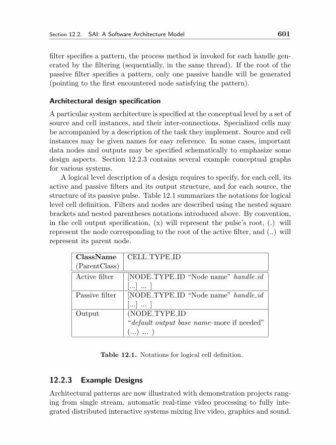
Section 12.2. SAI: A Software Architecture Model 601
filter specifies a pattern, the process method is invoked for each handle gen-erated by the filtering (sequentially, in the same thread). If the root of thepassive filter specifies a pattern, only one passive handle will be generated(pointing to the first encountered node satisfying the pattern).
Architectural design specification
A particular system architecture is specified at the conceptual level by a set ofsource and cell instances, and their inter-connections. Specialized cells maybe accompanied by a description of the task they implement. Source and cellinstances may be given names for easy reference. In some cases, importantdata nodes and outputs may be specified schematically to emphasize somedesign aspects. Section 12.2.3 contains several example conceptual graphsfor various systems.
A logical level description of a design requires to specify, for each cell, itsactive and passive filters and its output structure, and for each source, thestructure of its passive pulse. Table 12.1 summarizes the notations for logicallevel cell definition. Filters and nodes are described using the nested squarebrackets and nested parentheses notations introduced above. By convention,in the cell output specification, (x) will represent the pulse’s root, (.) willrepresent the node corresponding to the root of the active filter, and (..) willrepresent its parent node.
ClassName CELL TYPE ID(ParentClass)Active filter [NODE TYPE ID “Node name” handle id
[...] ... ]Passive filter [NODE TYPE ID “Node name” handle id
[...] ... ]Output (NODE TYPE ID
“default output base name–more if needed”(...) ... )
Table 12.1. Notations for logical cell definition.
12.2.3 Example Designs
Architectural patterns are now illustrated with demonstration projects rang-ing from single stream, automatic real-time video processing to fully inte-grated distributed interactive systems mixing live video, graphics and sound.
602 Software Architecture for Computer Vision Chapter 12
The projects are tentatively presented in order of increasing complexity, in-teractivity and cross-disciplinary integration. Each project is briefly intro-duced, its software architecture described and analyzed. Key architecturalpatterns, of general interest, are highlighted. These include feed-back loops,real-time incremental processing along the time dimension, interaction loops,real-time distributed processing, mixing and synchronization of multiple in-dependent data streams.
Real-Time Video Segmentation And Tracking
The development of real-time video analysis applications was actually a steer-ing concern during the development of the SAI style. The system presentedhere was used as a testbed for the implementation, testing and refinementof some fundamental SAI concepts [18].
The video analysis tasks performed are low level segmentation and blobtracking. The segmentation is performed by change detection using an adap-tive statistical color background model (the camera is assumed stationary).A review of background maintenance algorithms can be found in [28]. Blobtracking is performed using a new multi-resolution algorithm whose descrip-tion is out of the scope of this overview.
Figure 12.7 shows the conceptual level architecture of the software sys-tem. It is build around a single stream going through a number of cells. Thegraph can be decomposed into four functional subgraphs: capture, segmen-tation, tracking, visualization. The stream originates in the video input cell,which produces, at a given rate, pulses containing an image coming eitherfrom a live capture device or a video file. This cell and its source consti-tute the capture unit of the application. The stream then goes through thesegmentation unit, which is analyzed below. Coming out of the segmenta-tion, the stream goes through a tracking cell. The result visualization unitis composed of a rendering and a display subunits. Rendering of a persistentstructure (here, the tracking graph) will be illustrated in a more general con-text in another example below (“Live Video in Animated 3-D Graphics”).The display cell simply puts on the screen its input images, in this case thecomposite frames produced by the renderer.
A very interesting aspect of this system, and certainly the most innovativewhen it was introduced, is the asynchronous parallel implementation of thesegmentation algorithm, which contains a feed-back loop. The correspond-ing conceptual graph is also a flow graph of the algorithm. Each input frameis compared with a statistical background model. For each pixel, a decisionis made whether it is an observation of the background or of an occluding

Section 12.2. SAI: A Software Architecture Model 603
Live input
Background comparison
Connected components
Tracking Rendering
Display(composite image)
Background update
+ RGB input frame
+ foreground binary mask
+ labeled components image
+ composite image
Segmentation
BackgroundModel
TrackingGraph
Capture
Tracking
Display
Figure 12.7. Conceptual graph for real-time color background model-based seg-mentation and multi-resolution graph tracking application.
element. The output is a foreground binary mask. This comparison is per-formed by the background comparison cell. Each pulse, after going throughthis cell, contains the input image and a binary foreground image, whichis used by the connected components cell to produce a labeled componentsimage, added to the pulse. The input image and the labeled componentsimage are used by the background update cell to update the distributionsin the background model. Since the comparison and the update cells bothuse the persistent background model, they are both connected to a com-mon source that holds the background model structure. This path forms afeed back loop in which the result of the processing of each frame is used toupdate the adaptive background model. Because of the asynchrony of theprocessing, by the time the background model is updated with the result ofthe processing of a given frame, many other frames might have been com-pared to the model. In this particular context, the quality of the result is notaffected–in fact, it is common practice in background model maintenance toperform only partial updates at each frame, in order to reduce computationalload–and the overall system throughput permitted by this design is alwayssignificantly larger than that achievable in a sequential design. Another typeof parallelism is illustrated in the branching of the stream to follow indepen-dent parallel paths. After coming out of the connected components cell, the
604 Software Architecture for Computer Vision Chapter 12
stream follows a path to the update cell, and another path through trackingand finally visualization. While pulse-level multithreading principally im-proves throughput, stream-level parallelism has a major impact on latency.In this case, the result of the processing should be used as soon as possiblefor visualization and for update, in no arbitrarily imposed order. As longas computing resources (in a general sense) are available, and assuming fairscheduling, the model allows to achieve minimal latency.
Figure 12.8 shows two non consecutive frames from one of the PETS2002 [7] test sequences, with tracked blobs and their trajectories over a fewframes. Figure 12.9 presents three consecutive output frames obtained fromthe processing of professional racquetball videos. The ball and the playersare detected and tracked in real-time. In both cases, the original colors havebeen altered to highlight the blobs or the trajectories in the color to greyscale conversion required for printing.
Quantitative performance metrics are discussed below, in section 12.2.4.In the case of live video processing, the throughput of the system impactsthe quality of the results: a higher throughput allows the background modelto adapt to changing conditions more smoothly.
The modular architecture described here can be used to test differentalgorithms for each unit (e.g. segmentation algorithms) in an otherwisestrictly identical setting. It also constitute a foundation platform to whichhigher levels of processing can be added incrementally. The SAI style andits underlying data and processing models not only provide the necessaryarchitectural modularity for a test platform, but also the universal modelingpower to account for any algorithm, whether existing or yet to be formu-lated. In conjunction, the same platform also ensures that the best possibleperformance is achievable (provided correct architectural design and carefulimplementation of all the elements involved).
Real-Time Video Painting
The Video Painting project was developed as a demonstration of the real-time video stream processing ability provided by the SAI architectural style.It also provided valuable insight on the design and implementation of al-gorithms performing incremental processing along the time dimension, i.e.between different samples in a same stream.
The technical core of the application is a feature-based, multi-resolutionscheme to estimate frame to frame projective or affine transforms [21]. Thesetransforms are used to warp the frames to a common space to form a mosaic.The mosaic image itself is a persistent structure that evolves as more images

Section 12.2. SAI: A Software Architecture Model 605
Figure 12.8. Object segmentation and tracking results in a PETS02 test sequence.The examples shown are two sample output composite frames taken at differenttimes in the original video. The original colors have been altered to highlight thesegmented blobs (in white) in the color to grey scale conversion required for printing.
are processed, hence the name Video Painting.In a traditional sequential system, the transform between each pair of
consecutive frames would be computed, and each frame would be added tothe mosaic by combination of all the transforms between a reference frameand the current frame. Figure 12.10 shows the application graph for the SAIdesign. A live input unit creates the single stream, with frames captured froma camera. A simple cell computes the image pyramid associated with eachinput frame, and necessary for the multi-resolution frame-to-frame trans-form estimation performed by the next downstream cell. Comparing twosamples of the same stream requires to make one persistent, which becomesthe reference. Transforms are thus computed between the current frame anda reference frame. For the algorithm to work properly, though, the com-
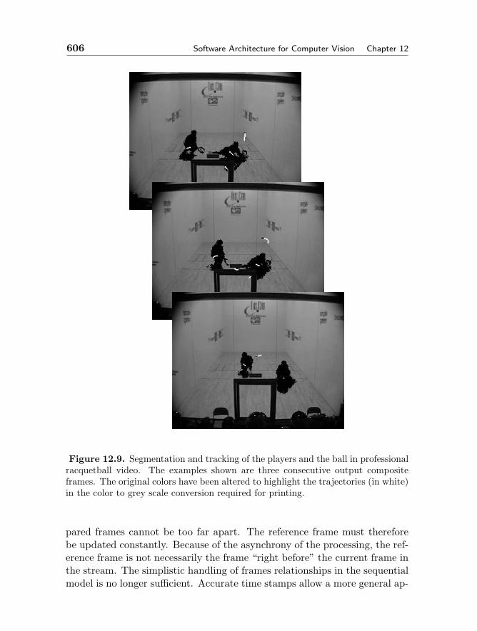
606 Software Architecture for Computer Vision Chapter 12
Figure 12.9. Segmentation and tracking of the players and the ball in professionalracquetball video. The examples shown are three consecutive output compositeframes. The original colors have been altered to highlight the trajectories (in white)in the color to grey scale conversion required for printing.
pared frames cannot be too far apart. The reference frame must thereforebe updated constantly. Because of the asynchrony of the processing, the ref-erence frame is not necessarily the frame “right before” the current frame inthe stream. The simplistic handling of frames relationships in the sequentialmodel is no longer sufficient. Accurate time stamps allow a more general ap-
Section 12.2. SAI: A Software Architecture Model 607
proach to the problem. The transforms computed between two frames are nolonger implicitly assumed to relate two consecutive frames, separated froma fixed time interval, but between two frames of arbitrary time stamps. Forefficiency reasons, the mosaic is also computed incrementally. A persistentimage containing the latest available version of the mosaic is maintained.Each new frame is warped and pasted on a copy of the mosaic by computingthe accumulated transform from the frame to the mosaic reference frame.To that effect, with the mosaic is also stored the accumulated transformfrom the time stamp of the reference mosaic frame to the time stamp of thelatest frame added, which is the time stamp for the mosaic. When a newframe is processed, the transform from the mosaic time stamp to the frameis computed by linear interpolation using the transform computed betweenthe frame and the reference frame. This is possible only because time is anexplicit component of the model. The transform is then composed with theaccumulated transform to produce a new accumulated transform, used towarp the current frame to mosaic space. After pasting of the warped frame,the updated mosaic image is copied into the persistent mosaic image to be-come the latest reference. The accumulated transform is also updated. Notethat a locking mechanism (e.g. critical section) is necessary to ensure consis-tency between the persistent mosaic and the accumulated transform as theyare accessed by different threads. In this design, the updated mosaic is alsoadded to the active pulse so that the dynamic stream of successive mosaicscan be viewed with an image display cell. Figure 12.11 shows two examplemosaics painted in real-time from a live video stream. The horizontal blacklines are image warping artifacts.
This application is an example where system latency and throughput di-rectly impact the quality of the results. The transform estimation processdegrades with the dissimilarity between the frames. A lower latency allowsfaster reference turnaround and thus smaller frame to frame dissimilarity.Higher throughput allows to build a finer mosaic. Embedding established al-gorithms into a more general parallel processing framework allows to achievehigh quality output in real-time. Furthermore, explicit handling of time rela-tionships in the design might give some insight on real-time implementationsof more complex mosaic building techniques, e.g. involving global constraintsto correct for registration error accumulation.
Handheld Mirror Simulation
The Virtual Mirror project [16, 15] started as a feasibility study for thedevelopment and construction of a handheld mirror simulation device.

608 Software Architecture for Computer Vision Chapter 12
Live input
Image pyramidcomputation
Transformestimation
Mosaic generation
Latest referenceimage
Latest mosaic
Display(mosaic)
+ input frame
+ image pyramid
+ transform
+ mosaic
Figure 12.10. Conceptual graph for Video Painting application (real-time mo-saicking).
The perception of the world reflected through a mirror depends on theviewer’s position with respect to the mirror and the 3-D geometry of theworld. In order to simulate a real mirror on a computer screen, images of theobserved world, consistent with the viewer’s position, must be synthesizedand displayed in real-time. This is of course geometrically impossible, butwith a few simplifying assumptions (e.g. planar world), the image transformrequired was made simple yet convincing enough to consider building anactual device. The current prototype system (see Figure 12.12) is comprisedof an LCD screen manipulated by the user, a single camera fixed on thescreen, and a tracking device. The continuous input video stream and trackerdata is used to synthesize, in real-time, a continuous video stream displayedon the LCD screen. The synthesized video stream is a close approximationof what the user would see on the screen surface if it were a real mirror.
Figure 12.13 shows the corresponding conceptual application graph. Thesingle stream application does not involve any complicated structure. Thestream originates in a live video input cell. A tracker input cell adds positionand orientation data to the stream. A mirror transform cell uses the syn-chronous image and tracking data to synthesize the mirror simulation image,which is then presented to the user by an image display cell.
The two major difficulties in this application are (1) synchronizing the
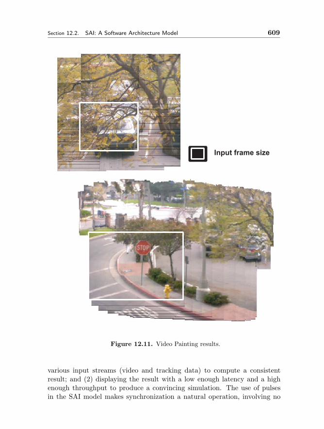
Section 12.2. SAI: A Software Architecture Model 609
Input frame size
Figure 12.11. Video Painting results.
various input streams (video and tracking data) to compute a consistentresult; and (2) displaying the result with a low enough latency and a highenough throughput to produce a convincing simulation. The use of pulsesin the SAI model makes synchronization a natural operation, involving no
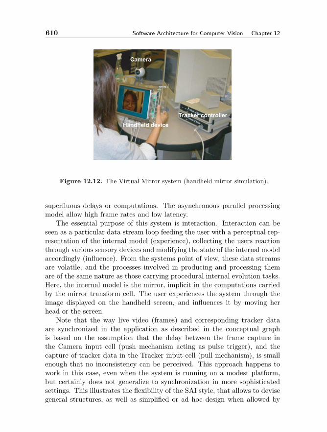
610 Software Architecture for Computer Vision Chapter 12
Camera
Tracker controller
Handheld device
Figure 12.12. The Virtual Mirror system (handheld mirror simulation).
superfluous delays or computations. The asynchronous parallel processingmodel allow high frame rates and low latency.
The essential purpose of this system is interaction. Interaction can beseen as a particular data stream loop feeding the user with a perceptual rep-resentation of the internal model (experience), collecting the users reactionthrough various sensory devices and modifying the state of the internal modelaccordingly (influence). From the systems point of view, these data streamsare volatile, and the processes involved in producing and processing themare of the same nature as those carrying procedural internal evolution tasks.Here, the internal model is the mirror, implicit in the computations carriedby the mirror transform cell. The user experiences the system through theimage displayed on the handheld screen, and influences it by moving herhead or the screen.
Note that the way live video (frames) and corresponding tracker dataare synchronized in the application as described in the conceptual graphis based on the assumption that the delay between the frame capture inthe Camera input cell (push mechanism acting as pulse trigger), and thecapture of tracker data in the Tracker input cell (pull mechanism), is smallenough that no inconsistency can be perceived. This approach happens towork in this case, even when the system is running on a modest platform,but certainly does not generalize to synchronization in more sophisticatedsettings. This illustrates the flexibility of the SAI style, that allows to devisegeneral structures, as well as simplified or ad hoc design when allowed by
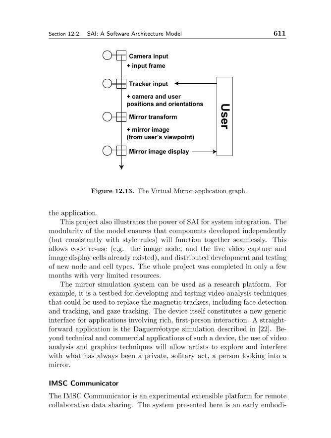
Section 12.2. SAI: A Software Architecture Model 611
Camera input
Tracker input
Mirror transform
Mirror image display
+ input frame
+ camera and userpositions and orientations
+ mirror image(from user’s viewpoint)
User
Figure 12.13. The Virtual Mirror application graph.
the application.This project also illustrates the power of SAI for system integration. The
modularity of the model ensures that components developed independently(but consistently with style rules) will function together seamlessly. Thisallows code re-use (e.g. the image node, and the live video capture andimage display cells already existed), and distributed development and testingof new node and cell types. The whole project was completed in only a fewmonths with very limited resources.
The mirror simulation system can be used as a research platform. Forexample, it is a testbed for developing and testing video analysis techniquesthat could be used to replace the magnetic trackers, including face detectionand tracking, and gaze tracking. The device itself constitutes a new genericinterface for applications involving rich, first-person interaction. A straight-forward application is the Daguerreotype simulation described in [22]. Be-yond technical and commercial applications of such a device, the use of videoanalysis and graphics techniques will allow artists to explore and interferewith what has always been a private, solitary act, a person looking into amirror.
IMSC Communicator
The IMSC Communicator is an experimental extensible platform for remotecollaborative data sharing. The system presented here is an early embodi-
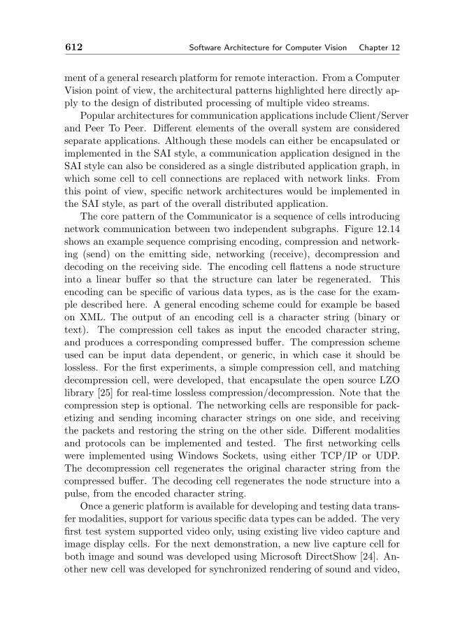
612 Software Architecture for Computer Vision Chapter 12
ment of a general research platform for remote interaction. From a ComputerVision point of view, the architectural patterns highlighted here directly ap-ply to the design of distributed processing of multiple video streams.
Popular architectures for communication applications include Client/Serverand Peer To Peer. Different elements of the overall system are consideredseparate applications. Although these models can either be encapsulated orimplemented in the SAI style, a communication application designed in theSAI style can also be considered as a single distributed application graph, inwhich some cell to cell connections are replaced with network links. Fromthis point of view, specific network architectures would be implemented inthe SAI style, as part of the overall distributed application.
The core pattern of the Communicator is a sequence of cells introducingnetwork communication between two independent subgraphs. Figure 12.14shows an example sequence comprising encoding, compression and network-ing (send) on the emitting side, networking (receive), decompression anddecoding on the receiving side. The encoding cell flattens a node structureinto a linear buffer so that the structure can later be regenerated. Thisencoding can be specific of various data types, as is the case for the exam-ple described here. A general encoding scheme could for example be basedon XML. The output of an encoding cell is a character string (binary ortext). The compression cell takes as input the encoded character string,and produces a corresponding compressed buffer. The compression schemeused can be input data dependent, or generic, in which case it should belossless. For the first experiments, a simple compression cell, and matchingdecompression cell, were developed, that encapsulate the open source LZOlibrary [25] for real-time lossless compression/decompression. Note that thecompression step is optional. The networking cells are responsible for pack-etizing and sending incoming character strings on one side, and receivingthe packets and restoring the string on the other side. Different modalitiesand protocols can be implemented and tested. The first networking cellswere implemented using Windows Sockets, using either TCP/IP or UDP.The decompression cell regenerates the original character string from thecompressed buffer. The decoding cell regenerates the node structure into apulse, from the encoded character string.
Once a generic platform is available for developing and testing data trans-fer modalities, support for various specific data types can be added. The veryfirst test system supported video only, using existing live video capture andimage display cells. For the next demonstration, a new live capture cell forboth image and sound was developed using Microsoft DirectShow [24]. An-other new cell was developed for synchronized rendering of sound and video,
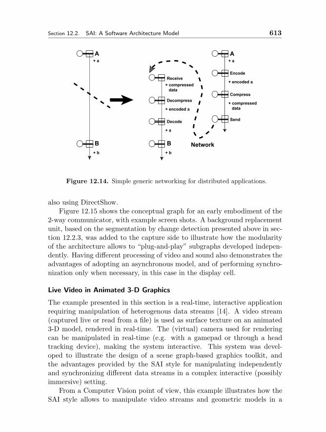
Section 12.2. SAI: A Software Architecture Model 613
A
Encode
Compress
Send
+ a
+ encoded a
+ compressed data
A
B
+ a
+ b
Receive
Decompress
Decode
+ compressed data
+ encoded a
+ a
B
+ b
Network
Figure 12.14. Simple generic networking for distributed applications.
also using DirectShow.Figure 12.15 shows the conceptual graph for an early embodiment of the
2-way communicator, with example screen shots. A background replacementunit, based on the segmentation by change detection presented above in sec-tion 12.2.3, was added to the capture side to illustrate how the modularityof the architecture allows to “plug-and-play” subgraphs developed indepen-dently. Having different processing of video and sound also demonstrates theadvantages of adopting an asynchronous model, and of performing synchro-nization only when necessary, in this case in the display cell.
Live Video in Animated 3-D Graphics
The example presented in this section is a real-time, interactive applicationrequiring manipulation of heterogenous data streams [14]. A video stream(captured live or read from a file) is used as surface texture on an animated3-D model, rendered in real-time. The (virtual) camera used for renderingcan be manipulated in real-time (e.g. with a gamepad or through a headtracking device), making the system interactive. This system was devel-oped to illustrate the design of a scene graph-based graphics toolkit, andthe advantages provided by the SAI style for manipulating independentlyand synchronizing different data streams in a complex interactive (possiblyimmersive) setting.
From a Computer Vision point of view, this example illustrates how theSAI style allows to manipulate video streams and geometric models in a
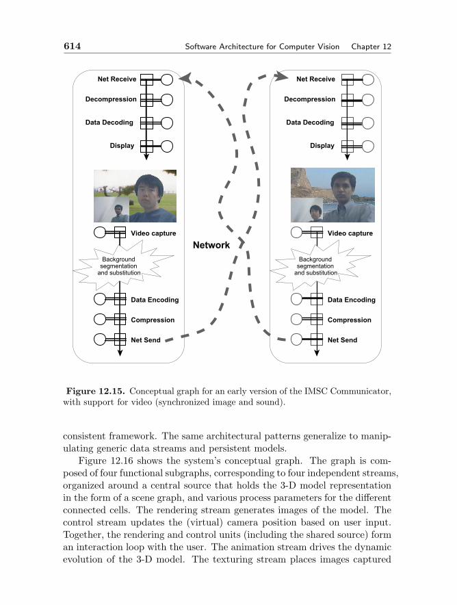
614 Software Architecture for Computer Vision Chapter 12
Data Encoding
Video capture
Compression
Net Send
Display
Net Receive
Decompression
Data Decoding
Data Encoding
Video capture
Compression
Net Send
Display
Net Receive
Decompression
Data Decoding
NetworkBackground
segmentationand substitution
Backgroundsegmentation
and substitution
Figure 12.15. Conceptual graph for an early version of the IMSC Communicator,with support for video (synchronized image and sound).
consistent framework. The same architectural patterns generalize to manip-ulating generic data streams and persistent models.
Figure 12.16 shows the system’s conceptual graph. The graph is com-posed of four functional subgraphs, corresponding to four independent streams,organized around a central source that holds the 3-D model representationin the form of a scene graph, and various process parameters for the differentconnected cells. The rendering stream generates images of the model. Thecontrol stream updates the (virtual) camera position based on user input.Together, the rendering and control units (including the shared source) forman interaction loop with the user. The animation stream drives the dynamicevolution of the 3-D model. The texturing stream places images captured

Section 12.2. SAI: A Software Architecture Model 615
from a video source (camera or file) in the texture node in the scene graph.Interaction and modeling are now analyzed in more detail.
Figure 12.16. Conceptual graph for integrating real-time rendering of an ani-mated 3-D model with live video mapping and interactive camera control.
Interaction As observed above, interaction is a particular data stream loopfeeding the user with a perceptual representation of the internal model (ex-perience), collecting the users reaction through various sensory devices andmodifying the state of the internal model accordingly (influence). From thesystems point of view, these data streams are volatile, and the processesinvolved in producing and processing them are of the same nature as thosecarrying procedural internal evolution tasks, and are thus modeled consis-tently in the SAI style.
Any such interaction subsystem, an example of which is the user loop onthe right half of figure 12.16, will involve instances of cells belonging to a fewtypical functional classes: inputs, effectors, renders, displays. Input collectuser input and generate the corresponding active pulses on streams. Thesecomponents encapsulate such devices as mouse, keyboard, 3-D tracker, etc.Effector cells use the input data to modify the state of the internal model(including possibly process parameters). In this example, the effector is thecamera control cell. In some cases, the data produced by the input devicerequires some processing in order to convert it into data that can be usedby the effector. This is the case for example with vision-based perceptualinterfaces, in which the input device is a camera, which produces a videostream that must be analyzed to extract the actual user input information.

616 Software Architecture for Computer Vision Chapter 12
Such processes can be implemented efficiently in the SAI style (see e.g. [18]),and be integrated consistently in an interactive application graph. Renderingand display elements produce and present a perceptual view of the internalmodel to the user, closing the loop. Display cells encapsulate output devices,such as screen image display, stereo image displays, sound output, etc. Notethat in some cases, e.g. for haptics, input and display functions are handledby the same device.
For interaction to feel natural, latency (or lag: the delay between inputaction and output response) must be kept below a threshold above whichthe user will perceive an inconsistency between her actions and the resultingsystem evolution. This threshold is dependent on the medium and on theapplication, but studies show that latency has a negative effect on humanperformance [23]. For example, human performance tests in virtual environ-ments with head-coupled display suggest a latency threshold of the order of200ms above which performance becomes worse, in terms of response time,than with static viewing [11]. The same study also suggests that latency hasa larger impact on performance than frame update rate. System throughput(including higher data bandwidth) is more related to the degree of immersive-ness, and could influence perceived latency. In any case, it is quite intuitiveand usually accepted that interactive systems can always benefit from lowerlatency and higher throughput. A careful design, an appropriate architectureand an efficient implementation are therefore critical in the development ofinteractive applications.
Renderers are an example of simultaneous manipulation of volatile andpersistent data. A rendering cell produces perceptual instantaneous snap-shots (volatile) of the environment (persistent) captured by a virtual devicesuch as microphone or camera, which is itself part of the environment model.The intrinsic parallelism and synchronization mechanism of the SAI style areparticularly well suited for well defined, consistent and efficient handling ofthese type of tasks. The rendering stream is generated by an instance ofthe Pulsar cell type, a fundamental specialized component that producesempty pulses on the stream at a given rate. In this example, the render-ing cell adds to the pulse an image of the 3-D model, synthesized using theOpenGL library. Persistent data used by the rendering, apart from the scenegraph, include a virtual camera, and rendering parameters such as the light-ing model used, etc. An image display cell puts the rendered frames on thescreen.
User input streams can follow either a pull or push model. In the pullapproach, which is used in this example, a Pulsar triggers a regular samplingof some input device encapsulated in a user input cell and corresponding
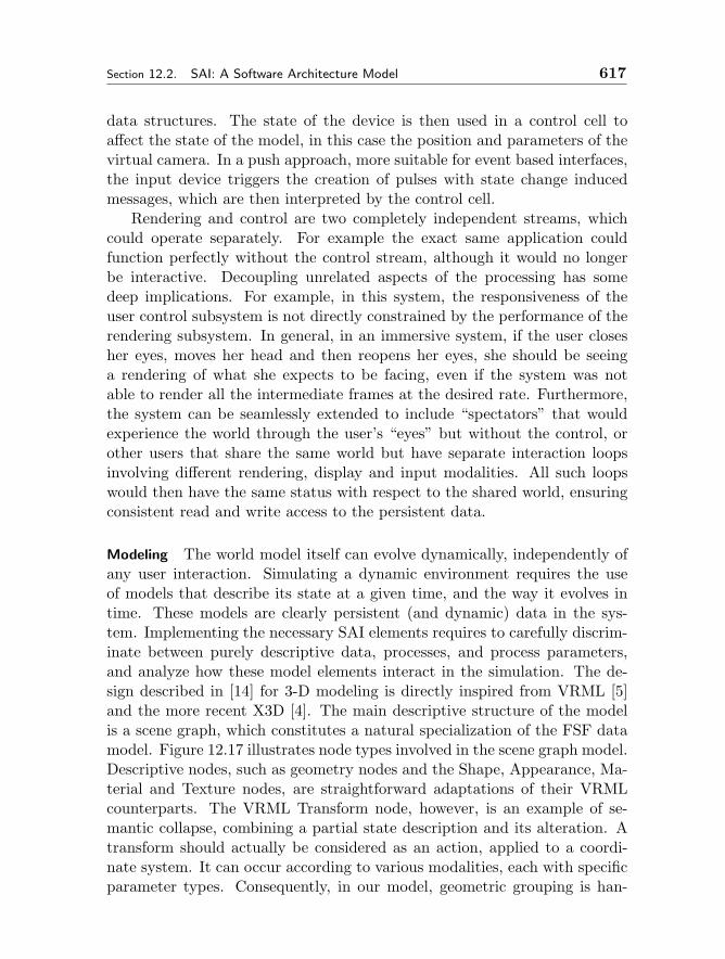
Section 12.2. SAI: A Software Architecture Model 617
data structures. The state of the device is then used in a control cell toaffect the state of the model, in this case the position and parameters of thevirtual camera. In a push approach, more suitable for event based interfaces,the input device triggers the creation of pulses with state change inducedmessages, which are then interpreted by the control cell.
Rendering and control are two completely independent streams, whichcould operate separately. For example the exact same application couldfunction perfectly without the control stream, although it would no longerbe interactive. Decoupling unrelated aspects of the processing has somedeep implications. For example, in this system, the responsiveness of theuser control subsystem is not directly constrained by the performance of therendering subsystem. In general, in an immersive system, if the user closesher eyes, moves her head and then reopens her eyes, she should be seeinga rendering of what she expects to be facing, even if the system was notable to render all the intermediate frames at the desired rate. Furthermore,the system can be seamlessly extended to include “spectators” that wouldexperience the world through the user’s “eyes” but without the control, orother users that share the same world but have separate interaction loopsinvolving different rendering, display and input modalities. All such loopswould then have the same status with respect to the shared world, ensuringconsistent read and write access to the persistent data.
Modeling The world model itself can evolve dynamically, independently ofany user interaction. Simulating a dynamic environment requires the useof models that describe its state at a given time, and the way it evolves intime. These models are clearly persistent (and dynamic) data in the sys-tem. Implementing the necessary SAI elements requires to carefully discrim-inate between purely descriptive data, processes, and process parameters,and analyze how these model elements interact in the simulation. The de-sign described in [14] for 3-D modeling is directly inspired from VRML [5]and the more recent X3D [4]. The main descriptive structure of the modelis a scene graph, which constitutes a natural specialization of the FSF datamodel. Figure 12.17 illustrates node types involved in the scene graph model.Descriptive nodes, such as geometry nodes and the Shape, Appearance, Ma-terial and Texture nodes, are straightforward adaptations of their VRMLcounterparts. The VRML Transform node, however, is an example of se-mantic collapse, combining a partial state description and its alteration. Atransform should actually be considered as an action, applied to a coordi-nate system. It can occur according to various modalities, each with specificparameter types. Consequently, in our model, geometric grouping is han-
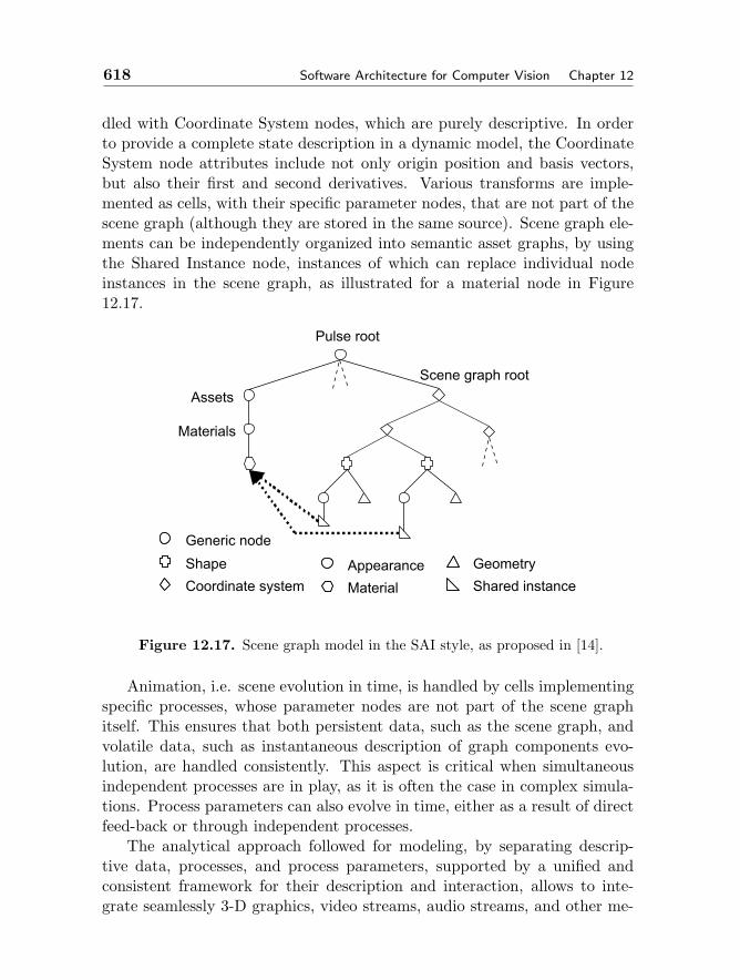
618 Software Architecture for Computer Vision Chapter 12
dled with Coordinate System nodes, which are purely descriptive. In orderto provide a complete state description in a dynamic model, the CoordinateSystem node attributes include not only origin position and basis vectors,but also their first and second derivatives. Various transforms are imple-mented as cells, with their specific parameter nodes, that are not part of thescene graph (although they are stored in the same source). Scene graph ele-ments can be independently organized into semantic asset graphs, by usingthe Shared Instance node, instances of which can replace individual nodeinstances in the scene graph, as illustrated for a material node in Figure12.17.
Scene graph root
Assets
Materials
Coordinate system
Shape Appearance Geometry
Material Shared instance
Generic node
Pulse root
Figure 12.17. Scene graph model in the SAI style, as proposed in [14].
Animation, i.e. scene evolution in time, is handled by cells implementingspecific processes, whose parameter nodes are not part of the scene graphitself. This ensures that both persistent data, such as the scene graph, andvolatile data, such as instantaneous description of graph components evo-lution, are handled consistently. This aspect is critical when simultaneousindependent processes are in play, as it is often the case in complex simula-tions. Process parameters can also evolve in time, either as a result of directfeed-back or through independent processes.
The analytical approach followed for modeling, by separating descrip-tive data, processes, and process parameters, supported by a unified andconsistent framework for their description and interaction, allows to inte-grate seamlessly 3-D graphics, video streams, audio streams, and other me-

Section 12.2. SAI: A Software Architecture Model 619
Figure 12.18. A rendered frame of the (animated) 3-D model with texturemapping from a live video stream.
dia types, as well as interaction streams. All these independent streams arein effect synchronized by the well defined and consistent use of shared data,in this case the scene graph and the virtual camera.
Figure 12.18 shows a rendered frame of a world composed of four spheresand four textured rectangles, rotating in opposite directions. Two fixedlights complete the model. A video stream captured live is used as texturefor the rectangles. Although this setting is not immersive (in the interest ofthe picture), the same system can easily made immersive by modifying thescene. The user may be placed in the center of the world, itself modeled by acylindrical polygonal surface on which a video stream, possibly pre-recordedfrom a panoramic camera system, is texture-mapped in real-time. The user,maybe using a head mounted display, only sees the part of the environmentshe is facing, and may control her viewing direction using a head tracker.
This application illustrates the flexibility and efficiency of the SAI archi-tectural style. In particular, thanks to the modularity of the framework, corepatterns (e.g. rendering, control, animation, etc.) can be effortlessly mixedand matched in a plug-and-play fashion to create systems with unlimitedvariations in the specific modalities (e.g. mouse or tracker input, screen orhead mounted display, etc.).
620 Software Architecture for Computer Vision Chapter 12
12.2.4 Architectural Properties
By design, the SAI style preserves many of the desirable properties identi-fied in the Pipes and Filters model. It allows intuitive design, emphasizingthe flow of data in the system. The graphical notation for conceptual levelrepresentations give a high level picture that can be refined as needed, downto implementation level, while remaining consistent throughout. The highmodularity of the model allows distributed development and testing of par-ticular elements, and easy maintenance and evolution of existing systems.The model also naturally supports distributed and parallel processing.
Unlike the Pipes and Filters style, the SAI style provides unified dataand processing models for generic data streams. It supports optimal (theo-retical) system latency and throughput thanks to an asynchronous parallelprocessing model. It provides a framework for consistent representation andefficient implementation of key processing patterns such as feed-back loopsand incremental processing along the time dimension. The SAI style hasseveral other important architectural properties that are out of the scope ofthis overview. These include natural support for dynamic system evolution,run-time reconfigurability, self monitoring, etc.
A critical architectural property that must be considered here is perfor-mance overhead. Some aspects of the SAI data and processing models, suchas filtering, involve non trivial computations, and could make the theory im-practical. The existence of fairly complex systems designed in the SAI styleand implemented with MFSM show that, at least for these examples, it isnot the case.
A closer look at how system performance is evaluated and reported isnecessary at this point. It is not uncommon to provide performance resultsin the form: “the system runs at n frames per second on a Processor X sys-tem at z K,M,GHz.” For example, the segmentation and tracking systempresented in the last section runs at 20 frames per second on 320x240 pixelsframes. The machine used is a dual processor Pentium 4 @ 1.7 GHz with1Go memory. Note that the system does not only perform segmentationand tracking: it also reads the frames from a file on disk or from a cam-era, produces a composite rendering of the analysis results, and displays theresulting images on the screen. In order to make the results reproducible,the hardware description should include the hard drive and/or camera andinterface, the graphics card, and how these elements interact with each other(e.g. the mother board specifications), etc. In practice, such a detailed de-scription of the hardware setting is tedious to put together, and probablyuseless, since reproducing the exact same setting would be difficult and even
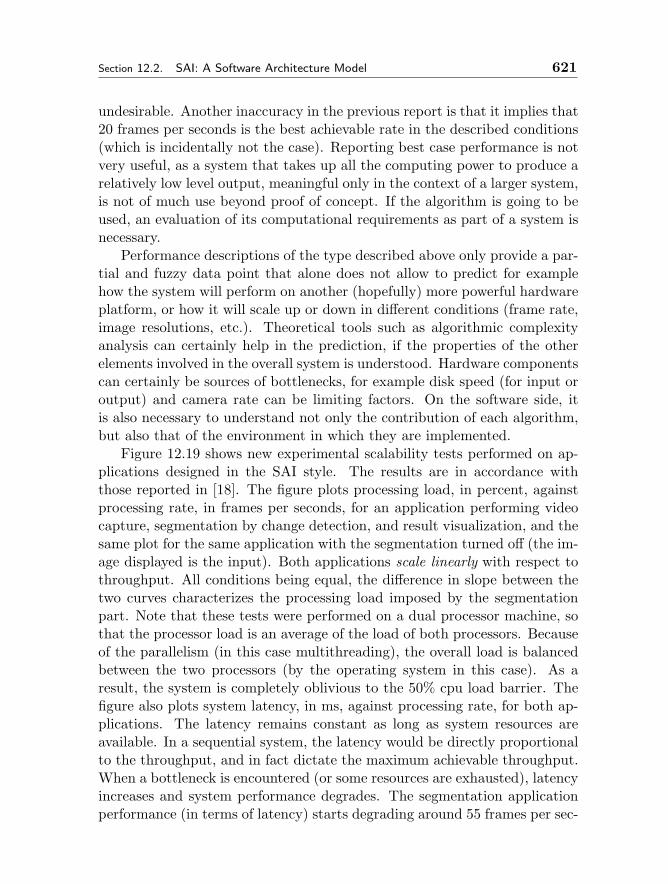
Section 12.2. SAI: A Software Architecture Model 621
undesirable. Another inaccuracy in the previous report is that it implies that20 frames per seconds is the best achievable rate in the described conditions(which is incidentally not the case). Reporting best case performance is notvery useful, as a system that takes up all the computing power to produce arelatively low level output, meaningful only in the context of a larger system,is not of much use beyond proof of concept. If the algorithm is going to beused, an evaluation of its computational requirements as part of a system isnecessary.
Performance descriptions of the type described above only provide a par-tial and fuzzy data point that alone does not allow to predict for examplehow the system will perform on another (hopefully) more powerful hardwareplatform, or how it will scale up or down in different conditions (frame rate,image resolutions, etc.). Theoretical tools such as algorithmic complexityanalysis can certainly help in the prediction, if the properties of the otherelements involved in the overall system is understood. Hardware componentscan certainly be sources of bottlenecks, for example disk speed (for input oroutput) and camera rate can be limiting factors. On the software side, itis also necessary to understand not only the contribution of each algorithm,but also that of the environment in which they are implemented.
Figure 12.19 shows new experimental scalability tests performed on ap-plications designed in the SAI style. The results are in accordance withthose reported in [18]. The figure plots processing load, in percent, againstprocessing rate, in frames per seconds, for an application performing videocapture, segmentation by change detection, and result visualization, and thesame plot for the same application with the segmentation turned off (the im-age displayed is the input). Both applications scale linearly with respect tothroughput. All conditions being equal, the difference in slope between thetwo curves characterizes the processing load imposed by the segmentationpart. Note that these tests were performed on a dual processor machine, sothat the processor load is an average of the load of both processors. Becauseof the parallelism (in this case multithreading), the overall load is balancedbetween the two processors (by the operating system in this case). As aresult, the system is completely oblivious to the 50% cpu load barrier. Thefigure also plots system latency, in ms, against processing rate, for both ap-plications. The latency remains constant as long as system resources areavailable. In a sequential system, the latency would be directly proportionalto the throughput, and in fact dictate the maximum achievable throughput.When a bottleneck is encountered (or some resources are exhausted), latencyincreases and system performance degrades. The segmentation applicationperformance (in terms of latency) starts degrading around 55 frames per sec-
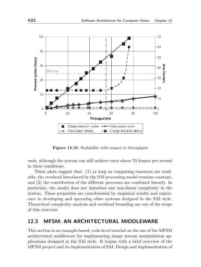
622 Software Architecture for Computer Vision Chapter 12
Figure 12.19. Scalability with respect to throughput.
onds, although the system can still achieve rates above 70 frames per secondin these conditions.
These plots suggest that: (1) as long as computing resources are avail-able, the overhead introduced by the SAI processing model remains constant,and (2) the contribution of the different processes are combined linearly. Inparticular, the model does not introduce any non-linear complexity in thesystem. These properties are corroborated by empirical results and experi-ence in developing and operating other systems designed in the SAI style.Theoretical complexity analysis and overhead bounding are out of the scopeof this overview.
12.3 MFSM: AN ARCHITECTURAL MIDDLEWARE
This section is an example-based, code-level tutorial on the use of the MFSMarchitectural middleware for implementing image stream manipulation ap-plications designed in the SAI style. It begins with a brief overview of theMFSM project and its implementation of SAI. Design and implementation of
Section 12.3. MFSM: An Architectural Middleware 623
applications for image stream manipulation is then explained in detail usingsimple examples, based on those used in the online MFSM user guide. Afirst example illustrates application setup and cleanup, application graph el-ements instantiation and connection. The development of specialized nodesis explained with a study of the implementation of a generic image datastructure (object of an open source module). The use of this node type ina specialized process is explained with a study of the implementation of acustom cell used in the first example. Finally, a more complex example il-lustrates shared memory access for incremental computations along the timedimension.
This section constitute an image-oriented, self contained complement tothe online user guide [12].
Disclaimer The code appearing in this section was developed by the author,and is part of open source modules and examples released under the GNULesser General Public License [1]. They are available for download on theMFSM web site [12]. This code is provided here in the hope that it will beuseful, but without any warranty; without even the implied warranty of mer-chantability or fitness for a particular purpose. Complete license informationis provided in the downloadable packages.
12.3.1 MFSM overview
MFSM (Modular Flow Scheduling Middleware) [12] is an architectural mid-dleware implementing the core elements of the SAI style. MFSM is an opensource project, released under the GNU Lesser General Public License [1].The goal of MFSM is to support and promote the design, analysis and im-plementation of applications in the SAI style. This goal is reflected in thedifferent facets of the project.
– The FSF library is an extensible set of implementation-level classesrepresenting the key elements of SAI. They can be specialized to definenew data structures and processes, or encapsulate existing ones (e.g.from operating system services and third-party libraries).
– A number of software modules regroup specializations implementingspecific algorithms or functionalities. They constitute a constantlygrowing base of open source, reusable code, maintained as part of theMFSM project. Related functional modules may be grouped into li-braries.
– An evolving set of example applications illustrates the use of FSF andspecific modules.
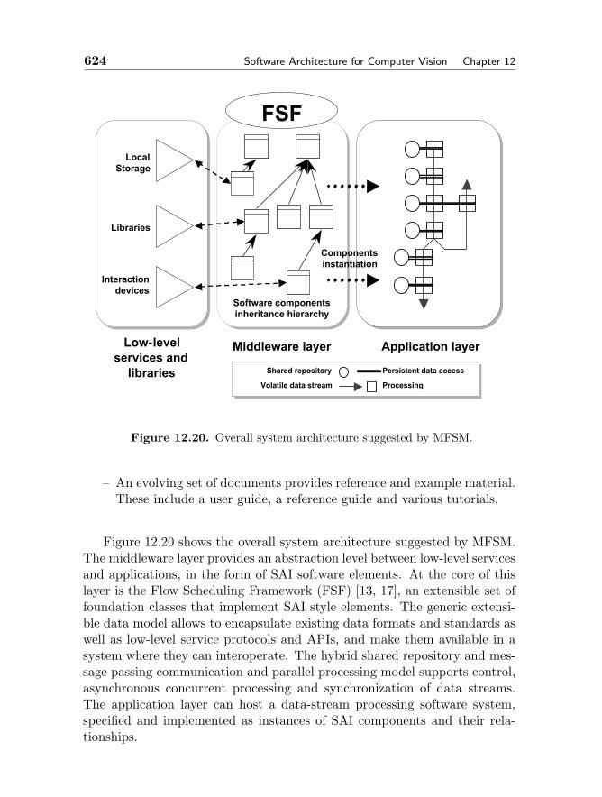
624 Software Architecture for Computer Vision Chapter 12
Application layerLow-level services and
libraries
Middleware layer
Software componentsinheritance hierarchy
Components instantiation
Interactiondevices
LocalStorage
Libraries
FSF
Shared repository Persistent data access
Volatile data stream Processing
Figure 12.20. Overall system architecture suggested by MFSM.
– An evolving set of documents provides reference and example material.These include a user guide, a reference guide and various tutorials.
Figure 12.20 shows the overall system architecture suggested by MFSM.The middleware layer provides an abstraction level between low-level servicesand applications, in the form of SAI software elements. At the core of thislayer is the Flow Scheduling Framework (FSF) [13, 17], an extensible set offoundation classes that implement SAI style elements. The generic extensi-ble data model allows to encapsulate existing data formats and standards aswell as low-level service protocols and APIs, and make them available in asystem where they can interoperate. The hybrid shared repository and mes-sage passing communication and parallel processing model supports control,asynchronous concurrent processing and synchronization of data streams.The application layer can host a data-stream processing software system,specified and implemented as instances of SAI components and their rela-tionships.
Section 12.3. MFSM: An Architectural Middleware 625
In its current implementation, the FSF library contains a set of C++classes implementing SAI elements: the source, the nodes and pulses, thecells, the filters, the handles. It also contains classes for two implementationrelated object types: the factories and the System. A brief overview ofeach object type is proposed below. An online reference guide [12] providesdetailed interface description and implementation notes for all the classesdefined in the FSF library.
Source The source class is fairly simple. It holds a single passive pulse,and keeps a list of pointers to connected cells. Note that connectors are notimplemented as objects, but simply lists of pointers in the components. Thisresults from the simplicity of the role played by connectors in the SAI style.In particular, they do not perform any computation. Sources also performgarbage collecting on their passive pulse when notified of a structural changeby a connected cell.
Nodes and pulses The FSF library contains a base node class, that imple-ments connectivity elements for building hierarchical structures. Specializednode classes, encapsulating or implementing specific data structures, will bederived from the base class. In FSF, from The base node class are derivedtwo specific classes for active and passive pulse respectively. These serveas root nodes for active and passive pulse which are node hierarchies. An-other node specialization is provided in FSF, that implements nodes holdingatomic type values (integer, floating point, boolean, string, etc.). These arecalled TypeNodes, and are implemented as template instances of a templateclasse, itself derived from a non template TypeNodeBase class (to allow un-determined pointers to a TypeNode object).
Cells The FSF library contains a base cell class, that implements cell-celland cell-source connectivity mechanisms (lists of pointers). It also imple-ments all the computation associated with the parallel processing of activepulses. In MFSM, in each cell, each active pulse is processed in a sepa-rate thread. Each passive filtering operation is also carried in a separatethread. As a result, some precautions must be taken for concurrent dataaccess. Thanks to inheritance and virtual functions, when implementinga specialized cell derived from the base cell, only the specific computationmust be coded, in an overloaded process virtual member funtion. All theevents leading to the call to this process function, including filtering, willbe automatically performed. A cell can be active or inactive. For efficiencypurposes, passive filtering only occurs when the cell is activated (activationfails if passive filtering fails), and when explicitely notified by the source,after a cell notified the source of a structural change in the passive pulse.
626 Software Architecture for Computer Vision Chapter 12
Filters Two sets of classes are implemented, for active and passive filters re-spectively. For each, a template class derived from a non template base classprovides support for intantiating filters corresponding to any node type. Thenon template base class allows to have pointers to undetermined filters (e.g.in cells). The filter objects also implement the filtering functionality. Ac-tive filtering instantiates and returns a list of active handles, passive filteringinstantiates and returns a list of passive handles.
Handles Two sets of classes are implemented, for active and passive handlesrespectively. Active handle simply provide a pointer to a node in an activepulse. An optional handle ID, inherited during the filtering operation, allowsto identify the node with respect to the filter. Passive handles play theadditional role of locks for node deletion and garbage collecting (not requiredin active pulses). When a cell removes a node, it does not destroy it, butmarks it as deleted, so it is not used in subsequent filtering operations. Thecell must notify the source, which in turns notify all connected cells to re-filter the passive pulse, and initiates a garbage collecting process, which willphysically deleted the node when is it free of handles from ongoing process.
Factories Class factories are used to instantiate objects at run time, whosetype is not known at compile time. Since cells and nodes constitute extensiblesets of specialized object types derived from respective base classes, Cell andNode factories a necessary for instantiating cells and nodes at run time,and modify application graphs dynamically. Node factories also allow toinstantiate filters for the corresponding node type.
System By convention, any application using FSF must have a single in-stance of the System type, a pointer to which is available as a global variable,defined in the FSF library. This object provides the reference clock, and holdsthe lists of node and cell factories available for building application graphs.In order to use a module in an application, its node and cell factories mustbe declared and registered with the system instance.
12.3.2 A First Image Manipulation Example
The online MFSM user guide [12] describes a simple program (called ex1)that generates a stream at a given frame rate, and displays the time stampof each pulse in both ms and in h/m/s formats. The example in this sectionperforms a similar task, but instead of being written to the standard output,each formatted time stamp string is written into a newly created image (usingIntel’s OpenCV [2]). This first example will be called eximg1.

Section 12.3. MFSM: An Architectural Middleware 627
Application design and specifications.
Before building a design, and after identifying the system requirements, it isuseful to know what building elements are available. This simple applicationinvolves a (single) stream, so the first concern is the origin of the stream.FSF contains a fundamental cell type that generates empty pulses at a givenframe rate. It is called Pulsar, and table 12.2 shows its specifications. Itdoes not have any input. It has one parameter, of integral type, whose valueis the time delay between two consecutive output pulses.
fsf::CPulsar FSF PULSAR(fsf::CCell)Active filter (no input)Passive filter [FSF INT32 NODE “Pulse delay”]Output (FSF ACTIVE PULSE “Root”)
Table 12.2. fsf::CPulsar logical cell definition.
In this section, it is assumed that a cell is available, that is capableof looking up the time stamp of each incoming active pulse, creating andimage, and printing the formatted time stamp in the image. The actualimplementation of this cell is addressed later, in the section 12.3.3. Table12.3 shows the cell specifications.
myspace::CMyCellImg MY CELL IMG(fsf::CCell)Active filter [FSF ACTIVE PULSE “Root”]Passive filter [FSF PASSIVE PULSE “Root”]Output (IMAGE IMAGE “Image”)
Table 12.3. myspace::MyCellImg logical cell definition.
The open source Display Module defines and implements a cell that candisplay an image into a window. Table 12.3 shows the ImageDisplay cellspecifications.
Given these elements, it is now straightforward to formulate a designfor eximg1, from one instance of Pulsar, one instance of MyCellImg andone instance of ImageDisplay. Figure 12.21 shows the resulting conceptualapplication graph.
The next few sections explain in detail how to code the simple application
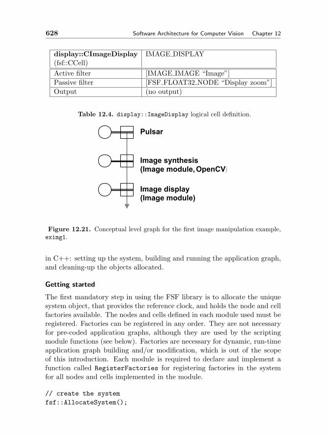
628 Software Architecture for Computer Vision Chapter 12
display::CImageDisplay IMAGE DISPLAY(fsf::CCell)Active filter [IMAGE IMAGE “Image”]Passive filter [FSF FLOAT32 NODE “Display zoom”]Output (no output)
Table 12.4. display::ImageDisplay logical cell definition.
Image synthesis(Image module, OpenCV)
Image display(Image module)
Pulsar
Figure 12.21. Conceptual level graph for the first image manipulation example,eximg1.
in C++: setting up the system, building and running the application graph,and cleaning-up the objects allocated.
Getting started
The first mandatory step in using the FSF library is to allocate the uniquesystem object, that provides the reference clock, and holds the node and cellfactories available. The nodes and cells defined in each module used must beregistered. Factories can be registered in any order. They are not necessaryfor pre-coded application graphs, although they are used by the scriptingmodule functions (see below). Factories are necessary for dynamic, run-timeapplication graph building and/or modification, which is out of the scopeof this introduction. Each module is required to declare and implement afunction called RegisterFactories for registering factories in the systemfor all nodes and cells implemented in the module.
// create the systemfsf::AllocateSystem();
Section 12.3. MFSM: An Architectural Middleware 629
// register system factoriesfsf::RegisterFactories();
// register module factoriesimage::RegisterFactories();display::RegisterFactories();
// register myspace factoriesmyspace::RegisterFactories();
Building the graph
A scripting module (namespace scripting) provides shortcut functions toinstantiate sources and cells, instantiate nodes and place them in sourcepulses, connect cells to other cells and to sources. The convention followedin the parameter order for stream connections is to plug a downstream cellinto an upstream cell. The name “scripting” comes from the fact that thefunctions provided by this module are coding equivalents of user actions inan interactive system. In particular, the scripting module uses aspects of theMFSM implementation that are related to dynamic system evolution, suchas class factories. Note that the scripting module itself does not implementany node or cell class and thus does not register any factory (there is noscripting::RegisterFactories).
The code for building an application graph instantiates and connects allthe elements of the conceptual graph. In this simple example, the graphcan be divided into three functional parts: the pulsing unit built aroundthe Pulsar instance, the image synthesis unit built around the MyCellImginstance, and the display unit built around the ImageDisplay instance. Eachsubgraph in this case corresponds to one source and one cell (minimal com-puting units).
Each minimal unit, consisting of one cell and one source whose pulsecontains the cell’s parameters, can be coded following these steps:
– Instantiate the source.
– Instantiate the parameter node(s). Each node is placed in the source’spassive pulse hierarchy. Optional steps for each node include settingits name and data member initial values.
– Instantiate the cell. Optional steps include setting the output basename, the active and passive filters. The cell is then connected to its

630 Software Architecture for Computer Vision Chapter 12
source, and to the cell directly upstream on the active stream, if any.
These principles can be used as guidelines and adapted to code any graph.The following code builds the graph for the example, first the pulsar unit,then the image synthesis unit, and finally the image display unit. Success-ful instantiation of all graph elements is checked, as failure to register theappropriate factories will result in the failure to instantiate a given cell ornode.
// build graphbool bSuccess=true;
/////////////////// Pulsar unit ///////////////////
// create the sourcefsf::CSource *pPSource=new fsf::CSource;bSuccess &= (pPSource!=NULL);
// parameter node: pulse delayfsf::Int32Node *pPulseDelay =static_cast<fsf::Int32Node*>(scripting::CreateNode(std::string("FSF_INT32_NODE"),pPSource->GetPulse()));
bSuccess &= (pPulseDelay!=NULL);if(bSuccess)// set namepPulseDelay->SetName(std::string("Pulse delay"));// set parameter valueslong nPulseDelay=static_cast<long>((1000.0f/fPulseRate)-1);pPulseDelay->SetData(nPulseDelay);
// cellfsf::CCell *pPcell =static_cast<fsf::CCell*>(scripting::CreateCell(std::string("FSF_PULSAR")));
bSuccess &= (pPcell!=NULL);if(bSuccess)
Section 12.3. MFSM: An Architectural Middleware 631
// connect with sourcescripting::ConnectSource(pPcell,pPSource);
//////////////////////////// Image synthesis unit ////////////////////////////
// create the sourcefsf::CSource *pMySource=new fsf::CSource;bSuccess &= (pMySource!=NULL);
// cellfsf::CCell *pMyCell =static_cast<fsf::CCell*>(scripting::CreateCell(std::string("MY_CELL_IMG")));
bSuccess &= (pMyCell!=NULL);if(bSuccess)// connect with sourcescripting::ConnectSource(pMyCell,pMySource);
// connect with Pcellscripting::ConnectUpstreamCell(pMyCell,pPcell);
//////////////////// Display unit ////////////////////
// create the sourcefsf::CSource *pDisplaySource=new fsf::CSource;bSuccess &= (pDisplaySource!=NULL);
// parameter node: display zoomfsf::Float32Node *pDisplayZoom=static_cast<fsf::Float32Node*>(scripting::CreateNode(std::string("FSF_FLOAT32_NODE"),pDisplaySource->GetPulse()));
bSuccess &= (pDisplayZoom!=NULL);if(bSuccess)

632 Software Architecture for Computer Vision Chapter 12
// set namepDisplayZoom->SetName(std::string("Display zoom"));// set parameter valuespDisplayZoom->SetData(1.0f);
// cellfsf::CCell *pDisplayCell =static_cast<fsf::CCell*>(scripting::CreateCell(std::string("IMAGE_DISPLAY")));
bSuccess &= (pDisplayCell!=NULL);if(bSuccess)// connect with sourcescripting::ConnectSource(pDisplayCell,pDisplaySource);
// connect with Pcellscripting::ConnectUpstreamCell(pDisplayCell,pMyCell);
// Check everything went OK...if(bSuccess==false)cout << "Some elements in the graph could not be instantiated."
<< endl;return (-1);
Running the graph
Once the graph is completed, the cells must be activated. The Pulsar in-stance is the origin of the active stream and starts generating empty pulsesas soon as it is activated. The MyCellImg instance, once activated, will pro-cess incoming pulses in parallel, asynchronously. The ImageDisplay instancewill render the images produced by the MyCellImg instance on the screen.The cells can be started in any order.
// run the cellspMyCell->On();pPcell->On();
Section 12.3. MFSM: An Architectural Middleware 633
pDisplayCell->On();
Although this aspect is not evident in this simple example, cells canbe turned on and off at any time during the execution of the application,elements (sources and cells) can be connected and disconnected at any time,new ones can be created and existing ones destroyed at any time.
Because the Display Module relies on the Microsoft Windows Operat-ing System to display images on the screen, the console application mustexplicitly provide for a mechanism to dispatch and process messages forthe display window. The following code serves this purpose. At the sametime, the GetAsyncKeyState function is used to check whether the Q key ispressed, to exit the loop.
// message loop for windows// + check for ’Q’ key (VK_Q id 0x51) pressedMSG msg;while(((GetAsyncKeyState(0x51)&0x1)==0)
&& ::GetMessage( &msg, NULL, 0, 0))::TranslateMessage( &msg );::DispatchMessage( &msg );
This is the only MS Windows specific code in the application.
Clean-up
The following code stops the cells, disconnects and destroys the differentelements instantiated when building the graph, and finally deallocates theunique global FSF system instance. The scripting module provides high levelfunctions to disconnect cells and source.
// Stop the cellspPcell->Off();pMyCell->Off();pDisplayCell->Off();
// Clean upscripting::DisconnectSource(pPcell);scripting::DisconnectStream(pPcell);delete pPcell;
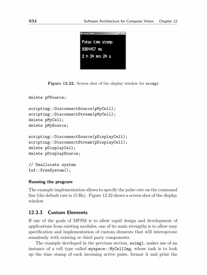
634 Software Architecture for Computer Vision Chapter 12
Figure 12.22. Screen shot of the display window for eximg1.
delete pPSource;
scripting::DisconnectSource(pMyCell);scripting::DisconnectStream(pMyCell);delete pMyCell;delete pMySource;
scripting::DisconnectSource(pDisplayCell);scripting::DisconnectStream(pDisplayCell);delete pDisplayCell;delete pDisplaySource;
// Deallocate systemfsf::FreeSystem();
Running the program
The example implementation allows to specify the pulse rate on the commandline (the default rate is 15 Hz). Figure 12.22 shows a screen shot of the displaywindow.
12.3.3 Custom Elements
If one of the goals of MFSM is to allow rapid design and development ofapplications from existing modules, one of its main strengths is to allow easyspecification and implementation of custom elements that will interoperateseamlessly with existing or third party components.
The example developed in the previous section, eximg1, makes use of aninstance of a cell type called myspace::MyCellImg, whose task is to lookup the time stamp of each incoming active pulse, format it and print the
Section 12.3. MFSM: An Architectural Middleware 635
resulting string into a newly created image. In this section, the designand implementation of specialized SAI elements (nodes and cells) is illus-trated on the customized elements of eximg1. First, the generic image nodeimage::CImage implemented in the open source Image Module is described.Then, the design and implementation of the myspace::MyCellImg cell type,which makes use of the image::CImage, are detailed step by step.
A custom node type: image::CImage
One solution when designing the image node was to encapsulate an existingimage structure. Unfortunately, each image processing library comes withits own image structure. Committing to a given library might prevent ac-cess to other libraries, and prove restrictive in the long term. The imagenode defined in the Image Module provides a minimum representation toensure its compatibility with existing image structures (in particular thatused in OpenCV). However the image node does contain any field specific ofparticular image formats, to ensure the widest compatibility. When needed,more specific image nodes may be derived from this base image node forleveraging specific library features. Because of inheritance properties, thesespecialized image nodes will be usable with all processes defined for the baseimage node.
Any node type specialization must be derived from the base node fsf::CNodeor a derived node. A node type is characterized by an identification string(used to link it to its factory). A complete node type description includes alist of data members and member functions, and a short description of itssemantics.
The image node is derived from the character buffer node defined in theFSF library. An image buffer is indeed a character buffer. The smallest setof parameters needed to make the character buffer usable as an image bufferare the image width and height, the number of channels and the pixel depth.Since some libraries require data line alignment for optimal performance, theactual aligned width (width step) must also be stored. A utility protectedmember function is used to compute the aligned width.
class CImage : public fsf::CCharBufferprotected:int m_nNbChannels; // Number of channelsint m_nDepth; // Pixel depth IMAGE_DEPTH_*
int m_nWidth; // Image width
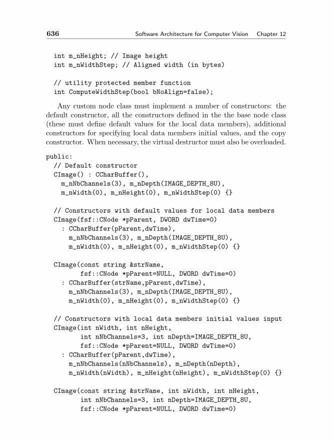
636 Software Architecture for Computer Vision Chapter 12
int m_nHeight; // Image heightint m_nWidthStep; // Aligned width (in bytes)
// utility protected member functionint ComputeWidthStep(bool bNoAlign=false);
Any custom node class must implement a number of constructors: thedefault constructor, all the constructors defined in the the base node class(these must define default values for the local data members), additionalconstructors for specifying local data members initial values, and the copyconstructor. When necessary, the virtual destructor must also be overloaded.
public:// Default constructorCImage() : CCharBuffer(),m_nNbChannels(3), m_nDepth(IMAGE_DEPTH_8U),m_nWidth(0), m_nHeight(0), m_nWidthStep(0)
// Constructors with default values for local data membersCImage(fsf::CNode *pParent, DWORD dwTime=0): CCharBuffer(pParent,dwTime),m_nNbChannels(3), m_nDepth(IMAGE_DEPTH_8U),m_nWidth(0), m_nHeight(0), m_nWidthStep(0)
CImage(const string &strName,fsf::CNode *pParent=NULL, DWORD dwTime=0)
: CCharBuffer(strName,pParent,dwTime),m_nNbChannels(3), m_nDepth(IMAGE_DEPTH_8U),m_nWidth(0), m_nHeight(0), m_nWidthStep(0)
// Constructors with local data members initial values inputCImage(int nWidth, int nHeight,
int nNbChannels=3, int nDepth=IMAGE_DEPTH_8U,fsf::CNode *pParent=NULL, DWORD dwTime=0)
: CCharBuffer(pParent,dwTime),m_nNbChannels(nNbChannels), m_nDepth(nDepth),m_nWidth(nWidth), m_nHeight(nHeight), m_nWidthStep(0)
CImage(const string &strName, int nWidth, int nHeight,int nNbChannels=3, int nDepth=IMAGE_DEPTH_8U,fsf::CNode *pParent=NULL, DWORD dwTime=0)
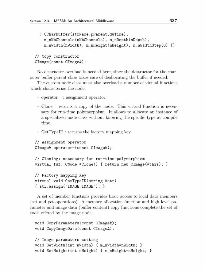
Section 12.3. MFSM: An Architectural Middleware 637
: CCharBuffer(strName,pParent,dwTime),m_nNbChannels(nNbChannels), m_nDepth(nDepth),m_nWidth(nWidth), m_nHeight(nHeight), m_nWidthStep(0)
// Copy constructorCImage(const CImage&);
No destructor overload is needed here, since the destructor for the char-acter buffer parent class takes care of deallocating the buffer if needed.
The custom node class must also overload a number of virtual functionswhich characterize the node:
– operator= : assignment operator.
– Clone : returns a copy of the node. This virtual function is neces-sary for run-time polymorphism. It allows to allocate an instance ofa specialized node class without knowing the specific type at compiletime.
– GetTypeID : returns the factory mapping key.
// Assignment operatorCImage& operator=(const CImage&);
// Cloning: necessary for run-time polymorphismvirtual fsf::CNode *Clone() return new CImage(*this);
// Factory mapping keyvirtual void GetTypeID(string &str) str.assign("IMAGE_IMAGE");
A set of member functions provides basic access to local data members(set and get operations). A memory allocation function and high level pa-rameter and image data (buffer content) copy functions complete the set oftools offered by the image node.
void CopyParameters(const CImage&);void CopyImageData(const CImage&);
// Image parameters settingvoid SetWidth(int nWidth) m_nWidth=nWidth; void SetHeight(int nHeight) m_nHeight=nHeight;
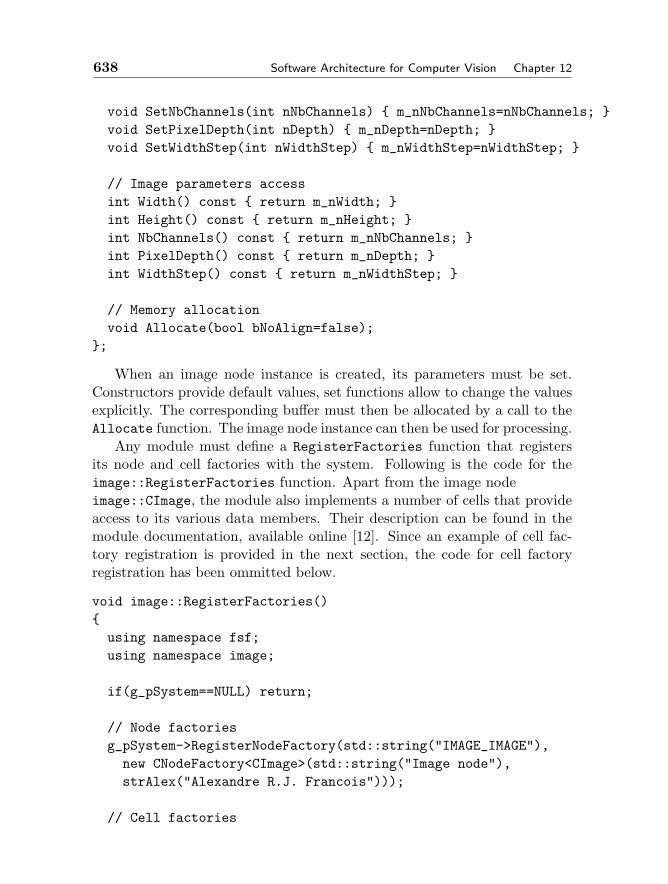
638 Software Architecture for Computer Vision Chapter 12
void SetNbChannels(int nNbChannels) m_nNbChannels=nNbChannels; void SetPixelDepth(int nDepth) m_nDepth=nDepth; void SetWidthStep(int nWidthStep) m_nWidthStep=nWidthStep;
// Image parameters accessint Width() const return m_nWidth; int Height() const return m_nHeight; int NbChannels() const return m_nNbChannels; int PixelDepth() const return m_nDepth; int WidthStep() const return m_nWidthStep;
// Memory allocationvoid Allocate(bool bNoAlign=false);
;
When an image node instance is created, its parameters must be set.Constructors provide default values, set functions allow to change the valuesexplicitly. The corresponding buffer must then be allocated by a call to theAllocate function. The image node instance can then be used for processing.
Any module must define a RegisterFactories function that registersits node and cell factories with the system. Following is the code for theimage::RegisterFactories function. Apart from the image nodeimage::CImage, the module also implements a number of cells that provideaccess to its various data members. Their description can be found in themodule documentation, available online [12]. Since an example of cell fac-tory registration is provided in the next section, the code for cell factoryregistration has been ommitted below.
void image::RegisterFactories()using namespace fsf;using namespace image;
if(g_pSystem==NULL) return;
// Node factoriesg_pSystem->RegisterNodeFactory(std::string("IMAGE_IMAGE"),new CNodeFactory<CImage>(std::string("Image node"),strAlex("Alexandre R.J. Francois")));
// Cell factories
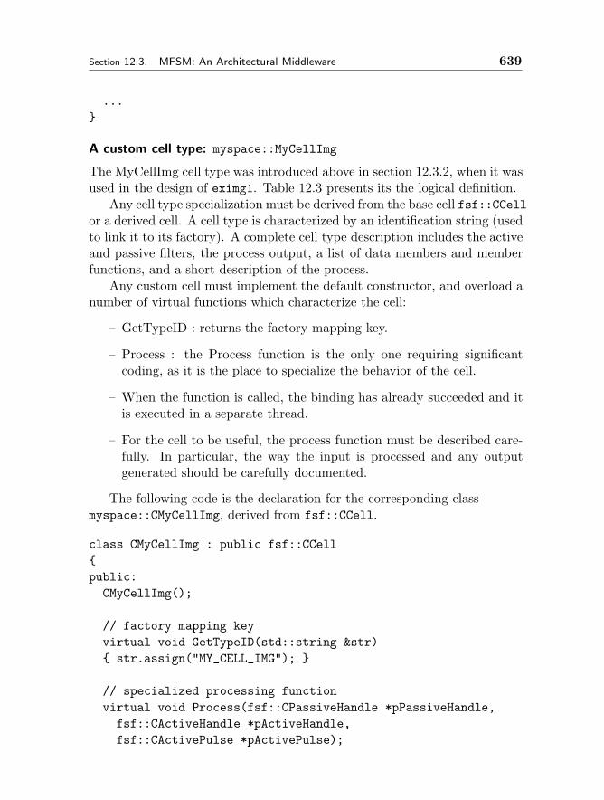
Section 12.3. MFSM: An Architectural Middleware 639
...
A custom cell type: myspace::MyCellImg
The MyCellImg cell type was introduced above in section 12.3.2, when it wasused in the design of eximg1. Table 12.3 presents its the logical definition.
Any cell type specialization must be derived from the base cell fsf::CCellor a derived cell. A cell type is characterized by an identification string (usedto link it to its factory). A complete cell type description includes the activeand passive filters, the process output, a list of data members and memberfunctions, and a short description of the process.
Any custom cell must implement the default constructor, and overload anumber of virtual functions which characterize the cell:
– GetTypeID : returns the factory mapping key.
– Process : the Process function is the only one requiring significantcoding, as it is the place to specialize the behavior of the cell.
– When the function is called, the binding has already succeeded and itis executed in a separate thread.
– For the cell to be useful, the process function must be described care-fully. In particular, the way the input is processed and any outputgenerated should be carefully documented.
The following code is the declaration for the corresponding classmyspace::CMyCellImg, derived from fsf::CCell.
class CMyCellImg : public fsf::CCellpublic:CMyCellImg();
// factory mapping keyvirtual void GetTypeID(std::string &str) str.assign("MY_CELL_IMG");
// specialized processing functionvirtual void Process(fsf::CPassiveHandle *pPassiveHandle,fsf::CActiveHandle *pActiveHandle,fsf::CActivePulse *pActivePulse);
640 Software Architecture for Computer Vision Chapter 12
;
The constructor sets the default output name base, and instantiates bothpassive and active filters from the corresponding template classes.
CMyCellImg::CMyCellImg(): CCell()// default output namem_strOutputName.assign("Image");// set the filtersm_pPassiveFilter =new fsf::CPassiveFilter<fsf::CPassivePulse>(std::string("Root"));
m_pActiveFilter =new fsf::CActiveFilter<fsf::CActivePulse>(std::string("Root"));
The specific behavior of a cell type is encoded in its overloaded processfunction. When the process function is executed, filtering of passive and ac-tive streams has succeeded. The active and passive handles are thus boundto the nodes satisfying the filters. When the filters are complex (i.e. hier-archies of filters), the passive and active handles point to their respectiveroots.
void CMyCellImg::Process(fsf::CPassiveHandle *pPassiveHandle,fsf::CActiveHandle *pActiveHandle,
fsf::CActivePulse *pActivePulse)
First, a pointer to the target node in the active pulse (in this case, theroot) is retrieved from the active handle. In this simple example, the processdoes not use any persistent data: the passive filter is defined such that thepassive handle points to the root of the passive pulse. There is no need toget an explicit pointer to this node.
fsf::CNode *pNode =static_cast<fsf::CNode*>(pActiveHandle->GetNode());
The node time stamp is retrieved using the fsf::CNode::GetTime func-tion. In this implementation, the time stamp is expressed in milliseconds.The equivalent time in hour/minute/second format is computed as follows:
Section 12.3. MFSM: An Architectural Middleware 641
long h=(pNode->GetTime()/3600000);long m=((pNode->GetTime()-h*3600000)/60000);long s=(pNode->GetTime()-h*3600000-m*60000)/1000;
The data to be output has been computed, it must now be placed intoan image. The output image, of type image::CImage, is created by a callto one of the constructors. The constructor sets the parent pointer in thenewly created node instance, but does not place the node in the parent’slist of subnodes. This will be done after all computations on the node havebeen completed. This ensures that eventual concurrent filtering processesnot take into account nodes that are not ready for use outside of the contextin which they were created. Note that the default output base name definedin fsf::CCell is a string object, and requires locking (using the associatedCriticalSection object) to avoid problems during concurrent access. Aftera call to the image node constructor, the image buffer is allocated, andinitialized with the value 0.
// Create imagem_csOutputName.Lock();image::CImage *pImage =new image::CImage(m_strOutputName,320,240,3,image::IMAGE_DEPTH_8U,pNode,fsf::g_pSystem->GetTime());
m_csOutputName.Unlock();
// Allocate bufferpImage->Allocate();// Fill in with 0memset(pImage->Data(),0,pImage->Size());
Once the image node instance is ready, it must be made available to theOpenCV functions, through an appropriate header. The code below createsan OpenCV image header corresponding to the image node parameters, anlinks the header to the actual image buffer.
// Use OpenCV
CvSize size;size.width=pImage->Width();size.height=pImage->Height();
642 Software Architecture for Computer Vision Chapter 12
// Create IPL image headerIplImage *pIplImage =cvCreateImageHeader(size,IPL_DEPTH_8U,pImage->NbChannels());
// Link image datapIplImage->imageData=pImage->Data();pIplImage->origin=IPL_ORIGIN_BL;
The various results are placed into formatted character strings, which areprinted in the image using the OpenCV cvPutText function.
CvFont font;cvInitFont(&font,CV_FONT_VECTOR0,0.8,0.8,0.0,2.0);
char str[255];sprintf(str,"Pulse time stamp:");cvPutText(pIplImage,str,cvPoint(15,200),&font,
CV_RGB(255,255,255));
sprintf(str,"%d ms",pNode->GetTime());cvPutText(pIplImage,str,cvPoint(15,150),&font,
CV_RGB(255,255,255));
sprintf(str,"%d h %2d min %2d s",h,m,s);cvPutText(pIplImage,str,cvPoint(15,100),&font,
CV_RGB(255,255,255));
When done with using OpenCV, the image header can be deleted. Notethat only the header is deleted, as the image node (including its image buffer)is the product of the process function.
cvReleaseImageHeader(&pIplImage);
Finally, all computations on the image node being completed, the nodecan be registered in its parent’s list of subnodes.
pNode->AddComponent(pImage);
At this point, the newly created imge node is part of the active pulse.When the process function returns, a number of operations are then carriedby the cell, resulting in the transmission of the augmented active pulse to alldownstream cells.
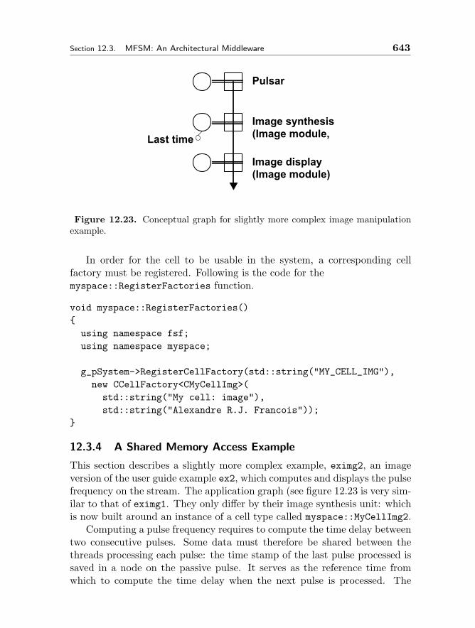
Section 12.3. MFSM: An Architectural Middleware 643
Pulsar
Image synthesis(Image module,
Image display(Image module)
Last time
Figure 12.23. Conceptual graph for slightly more complex image manipulationexample.
In order for the cell to be usable in the system, a corresponding cellfactory must be registered. Following is the code for themyspace::RegisterFactories function.
void myspace::RegisterFactories()using namespace fsf;using namespace myspace;
g_pSystem->RegisterCellFactory(std::string("MY_CELL_IMG"),new CCellFactory<CMyCellImg>(std::string("My cell: image"),std::string("Alexandre R.J. Francois"));
12.3.4 A Shared Memory Access Example
This section describes a slightly more complex example, eximg2, an imageversion of the user guide example ex2, which computes and displays the pulsefrequency on the stream. The application graph (see figure 12.23 is very sim-ilar to that of eximg1. They only differ by their image synthesis unit: whichis now built around an instance of a cell type called myspace::MyCellImg2.
Computing a pulse frequency requires to compute the time delay betweentwo consecutive pulses. Some data must therefore be shared between thethreads processing each pulse: the time stamp of the last pulse processed issaved in a node on the passive pulse. It serves as the reference time fromwhich to compute the time delay when the next pulse is processed. The

644 Software Architecture for Computer Vision Chapter 12
following code instantiates and connects the elements of the image synthesisunit for eximg2. Thanks to the modularity of SAI, this image synthesis unitdirectly replaces that of the previous example, without any modification tothe rest of the application graph.
//////////////////////////// Image synthesis unit ////////////////////////////
// create the sourcefsf::CSource *pMySource=new fsf::CSource;bSuccess &= (pMySource!=NULL);
// last time stampfsf::Int32Node *pLastTime =static_cast<fsf::Int32Node*>(scripting::CreateNode(std::string("FSF_INT32_NODE"),pMySource->GetPulse()));
bSuccess &= (pLastTime!=NULL);if(bSuccess)// set namepLastTime->SetName(std::string("Last time"));
// cellfsf::CCell *pMyCell =static_cast<fsf::CCell*>(scripting::CreateCell(std::string("MY_CELL_IMG2")));
bSuccess &= (pMyCell!=NULL);if(bSuccess)// connect with sourcescripting::ConnectSource(pMyCell,pMySource);
// connect with Pcellscripting::ConnectUpstreamCell(pMyCell,pPcell);
The myspace::MyCellImg2 cell type is in appearance quite similar tomyspace::MyCellImg. Table 12.5 shows its logical definition.

Section 12.3. MFSM: An Architectural Middleware 645
myspace::CMyCellImg2 MY CELL IMG2(fsf::CCell)Active filter [FSF ACTIVE PULSE “Root”]Passive filter [FSF INT32 NODE “Last time”]Output (IMAGE IMAGE “Image”)
Table 12.5. myspace::MyCellImg2 logical cell definition.
The difference in the passive filter is reflected in the constructor code, asfollows.
CMyCellImg2::CMyCellImg2(): CCell()// default output namem_strOutputName.assign("Image");// set the filtersm_pPassiveFilter =new fsf::CPassiveFilter<fsf::Int32Node>(std::string("Last time"));
m_pActiveFilter =new fsf::CActiveFilter<fsf::CActivePulse>(std::string("Root"));
The overloaded process function encodes the specific behavior of themyspace::MyCellImg2 cell type.
void CMyCellImg2::Process(fsf::CPassiveHandle *pPassiveHandle,fsf::CActiveHandle *pActiveHandle,fsf::CActivePulse *pActivePulse)
First a pointer to the target node in the passive pulse is retreived fromthe passive handle. In this case, it is a node of type fsf::Int32Node, whichcontains the value of the last time stamp read. Initialization of this value ishandled in the reset case described below.
fsf::Int32Node *pLastTime =static_cast<fsf::Int32Node*>(pPassiveHandle->GetNode());

646 Software Architecture for Computer Vision Chapter 12
A pointer to the target node in the active pulse, in this case the root ofthe pulse, is also retrieved, from the active handle.
fsf::CNode *pNode =static_cast<fsf::CNode*>(pActiveHandle->GetNode());
The first time this process function is executed, the passive node contain-ing the last time stamp value must be set to the value of the time stamp ofthe current active pulse, and no significant time difference can be produced.This section will be executed each time the m bReset flag, data member ofthe fsf::CCell class, is set to true.
if(m_bReset)pLastTime->SetData(pNode->GetTime());m_bReset=false;
When the reset flag is not set, the regular processing is carried as follows.
else
First and foremost, the value of the last time stamp is collected fromthe passive node. The value in the node is updated immediately with thecurrent time stamp value, so that it is available as soon as possible for even-tual parallel processes. In a strict parallel implementation, this read/writesequence should be placed in a critical section. In this simple example, thepossible side effect is neglected. It can be made apparearent by increasingthe requested throughput until it becomes too high for the system on whichthe application is running. The throughput computed by this cell then be-comes an integer fraction of the actual throughput because the reading andthe updating sequence of the time stamp values is no longer in effect atomic.
DWORD dwLastTime=pLastTime->GetData();pLastTime->SetData(static_cast<long>(pNode->GetTime()));
The remainder of the function code is quite similar to that ofCMyCellImg::Process. The output image is created, its data buffer allo-cated and set to 0.

Section 12.3. MFSM: An Architectural Middleware 647
m_csOutputName.Lock();image::CImage *pImage =new image::CImage(m_strOutputName,320,240,
3,image::IMAGE_DEPTH_8U,pNode,fsf::g_pSystem->GetTime());
m_csOutputName.Unlock();
pImage->Allocate();memset(pImage->Data(),0,pImage->Size());
A corresponding OpenCV header is created and linked to the image databuffer.
// Use OpenCV
CvSize size;size.width=pImage->Width();size.height=pImage->Height();
// Create IPL image headerIplImage *pIplImage =cvCreateImageHeader(size,IPL_DEPTH_8U,pImage->NbChannels());
// Link image datapIplImage->imageData=pImage->Data();pIplImage->origin=IPL_ORIGIN_BL;
Computed values are placed in a string, which is then written in theimage buffer using the OpenCV cvPutText function.
CvFont font;cvInitFont(&font,CV_FONT_VECTOR0,0.8,0.8,0.0,2.0);
char str[255];sprintf(str,"Pulse delay:");cvPutText(pIplImage,str,cvPoint(15,200),&font,
CV_RGB(255,255,255));
sprintf(str,"%d ms",pNode->GetTime()-dwLastTime);cvPutText(pIplImage,str,cvPoint(15,150),&font,
CV_RGB(255,255,255));
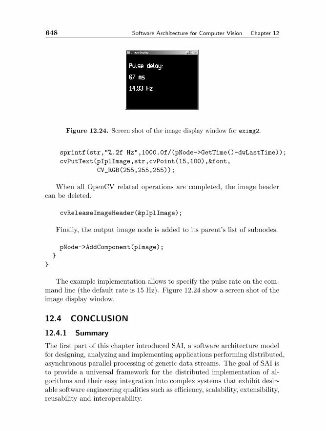
648 Software Architecture for Computer Vision Chapter 12
Figure 12.24. Screen shot of the image display window for eximg2.
sprintf(str,"%.2f Hz",1000.0f/(pNode->GetTime()-dwLastTime));cvPutText(pIplImage,str,cvPoint(15,100),&font,
CV_RGB(255,255,255));
When all OpenCV related operations are completed, the image headercan be deleted.
cvReleaseImageHeader(&pIplImage);
Finally, the output image node is added to its parent’s list of subnodes.
pNode->AddComponent(pImage);
The example implementation allows to specify the pulse rate on the com-mand line (the default rate is 15 Hz). Figure 12.24 show a screen shot of theimage display window.
12.4 CONCLUSION
12.4.1 Summary
The first part of this chapter introduced SAI, a software architecture modelfor designing, analyzing and implementing applications performing distributed,asynchronous parallel processing of generic data streams. The goal of SAI isto provide a universal framework for the distributed implementation of al-gorithms and their easy integration into complex systems that exhibit desir-able software engineering qualities such as efficiency, scalability, extensibility,reusability and interoperability.

Section 12.4. Conclusion 649
SAI specifies a new architectural style (components, connectors and con-straints). The underlying extensible data model and hybrid (shared reposi-tory and message-passing) distributed asynchronous parallel processing modelallow natural and efficient manipulation of generic data streams, using ex-isting libraries or native code alike. The modularity of the style facilitatesdistributed code development, testing, and reuse, as well as fast system de-sign and integration, maintenance and evolution. A graph-based notation forarchitectural designs allows intuitive system representation at the conceptualand logical levels, while at the same time mapping closely to processes.
Architectural patterns were illustrated through a number of ComputerVision-related demonstration projects ranging from single stream automaticreal-time video processing to fully integrated distributed interactive systemsmixing live video, graphics, sound, etc. By design, the SAI style preservesdesirable properties identified in the classic Pipes and Filters model. Theseinclude modularity and natural support for parallelism. Unlike the Pipes andFilters model, the SAI style allows to achieve optimal (theoretical) systemlatency and throughput, and provides a unified framework for consistent rep-resentation and efficient implementation of fundamental processing patternssuch as feed-back loops and incremental processing along the time dimension.
The second part of the chapter was a code-level tutorial on MFSM, anarchitectural middleware implementing the SAI style. Its core element, theFSF library, is a set of extensible classes that can be specialized to definenew data structures and processes, or encapsulate existing ones (e.g. fromlibraries). MFSM is an open source project, released under the GNU LesserGeneral Public License. A number of software modules regroup specializa-tions implementing specific algorithms or functionalities. They constitute aconstantly growing base of open source, reusable code, maintained as part ofthe MFSM project. The project is also thoroughly documented, and com-prises a user guide, a reference guide and various tutorials.
Simple example applications illustrated the design and implementation ofimage stream manipulation applications using the SAI style and the MFSMmiddleware. In particular, the implementation of a generic image node (ob-ject of an open source module) and its use in conjunction with the OpenCVlibrary in specialized cells were described step by step.
12.4.2 Perspectives
The SAI architectural style exhibit properties that make it relevant to re-search, educational and even industrial projects .
Thanks to its modularity, it can accommodate today’s requirements while
650 Software Architecture for Computer Vision Chapter 12
preparing for tomorrow’s applications. Using the SAI style for research cannot only save time by avoiding to re-develop existing modules, it can alsoreduce the technology transfer time once the research has matured.
SAI also allows distributed development of functional modules, and theirseamless integration into complex systems. The modularity of the design alsoallows gradual development, facilitating continuing validation and naturallysupporting regular delivery of incremental system prototypes. A number ofcross-disciplinary research projects, in addition to those described above insection 12.2.3, are already leveraging these properties. They are producingreal-time, interactive systems spanning a range of research domains.
Using the SAI style for developments in research projects can also reducethe technology transfer time once the technology has matured. From anindustry point of view, the SAI style allows fast prototyping for proof-of-concept demonstrations.
For education, SAI allows to efficiently relate classroom projects to therealities of the research laboratory, and of industrial software development.A project-oriented Integrated Media Systems class based on SAI, and apply-ing the distributed development model, was taught at USC in the Fall 2002semester at the advance graduate level. Rather than having small teamsof students develop a same, simple complete project, the small teams firstimplemented complementary parts of an overall, much more complex project(distributed soccer game). After six weeks of distributed development, snac-tioned by careful incremental cross-testing, all the pieces were put togetherto produce a playable system. The course was an outstanding success, andregular graduate and undergraduate courses based on this model are in theplanning.
Beyond the ones highlighted in the context of this chapter, the SAIstyle has several important desirable architectural properties that make it apromising framework for many applications in various fields. These proper-ties include natural support for dynamic system evolution, run-time recon-figurability, self monitoring, etc. Application of SAI in various contexts iscurrently being explored (e.g. interactive immersive systems). Short termtechnical developments for SAI include development of a Graphical UserInterface for system architecture design. Architecture validation and moni-toring and analysis tools will be gradually integrated.
Finally, from a theoretical point of view, because of the explicit distinc-tion between volatile and persistent data, SAI is a unified computationalmodel that bridges the conceptual and practical gap between signal (datastream) processing on the one hand, and the computation of higher level data(persistent, dynamic structures) on the other hand. As such, it might prove
Section 12.5. Acknowledgments 651
to be not only a powerful tool for implementing, but also for modeling andreasoning about problems spanning both aspects. An example is ComputerVision.
12.5 ACKNOWLEDGMENTS
The following (then) graduate students were involved in some of the projectspresented in section 12.2.3: Dr. Elaine Kang (Video Painting, VirtualMirror), Maurya Shah (IMSC Communicator–networking and compression),Kevin Zhu (IMSC Communicator–video and sound capture and synchronizedrendering).
This work has been funded in part by the Integrated Media Systems Cen-ter, a National Science Foundation Engineering Research Center, Coopera-tive Agreement No. EEC-9529152. Any Opinions, findings and conclusionsor recommendations expressed in this material are those of the author(s) anddo not necessarily reflect those of the National Science Foundation.
This work was supported in part by the Advanced Research and Devel-opment Activity of the U.S. Government under contract No. MDA-908-00-C-0036.
Bibliography
[1] Gnu Lesser General Public License. URL http://www.gnu.org/copyleft/lesser.html.
[2] Intel Open Source Computer Vision Library. URL http://www.intel.com/research/mrl/research/opencv/.
[3] Visual surveillance resources. URL http://visualsurveillance.org.[4] X3D: Extensible 3D international draft standards, iso/iec fcd 19775:200x.
URL http://www.web3d.org/technicalinfo/specifications/ISO_IEC_19775/index.% html.
[5] VRML 97: The Virtual Reality Modeling Language, iso/iec 14772:1997,1997. URL http://www.web3d.org/technicalinfo/specifications/ISO_IEC_14772-All/in% dex.html.
[6] PETS01: Second IEEE International Workshop on Performance Evalua-tions of Tracking and Surveillance, December 2001. URL http://pets2001.visualsurveillance.org.
[7] PETS02: Third IEEE International Workshop on Performance Evalua-tions of Tracking and Surveillance, June 2002. URL http://pets2002.visualsurveillance.org.
[8] PETS-ICVS: Fourth IEEE International Workshop on Performance Evalua-tions of Tracking and Surveillance, March 2003. URL http://petsicvs.visualsurveillance.org.
652 Software Architecture for Computer Vision Chapter 12
[9] PETS-VS: Joint IEEE International Workshop on Visual Surveillance and Per-formance Evaluations of Tracking and Surveillance, October 2003. URL http://vspets.visualsurveillance.org.
[10] G. R. Andrews. Foundations of multithreaded, parallel and distributed program-ming. Addison Wesley, 2000.
[11] K. W. Arthur, K. S. Booth, and C. Ware. Evaluating 3d task performance forfish tank virtual worlds. ACM Transactions on Information Systems, 11(3):239–265, 1993.
[12] A. R.J. Francois. Modular Flow Scheduling Middleware. URL http://mfsm.sourceForge.net.
[13] A. R.J. Francois. Semantic, Interactive Manipulations of Visual Data. PhD the-sis, Dept. of Computer Science, University of Southern California, Los Angeles,CA, 2000.
[14] A. R.J. Francois. Components for immersion. In Proceedings of the IEEE Inter-national Conference on Multimedia and Expo. Lausanne, Switzerland, August2002.
[15] A. R.J. Francois and E. Kang. A handheld mirror simulation. In Proceedingsof the IEEE International Conference on Multimedia and Expo, pages Vol II:745–748. Baltimore, MD, July 2003.
[16] A. R.J. Francois, E. Kang, and U. Malesci. A handheld virtual mirror. In ACMSIGGRAPH Conference Abstracts and Applications proceedings, page 140. SanAntonio, TX, July 2002.
[17] A. R.J. Francois and G. G. Medioni. A modular middleware flow schedul-ing framework. In Proceedings of ACM Multimedia 2000, pages 371–374. LosAngeles, CA, November 2000.
[18] A. R.J. Francois and G. G. Medioni. A modular software architecture for real-time video processing. In Springer-Verlag, editor, IEEE International Workshopon Computer Vision Systems, pages 35–49. Vancouver, B.C., Canada, July2001.
[19] C. Jaynes, S. Webb, R. M. Steele, and Xiong Q. An open development envi-ronment for evaluation of video surveillance systems. In PETS02, pages 32–39.Copenhagen, Denmark, June 2002.
[20] M. B. Jones and J. Regehr. The problems you’re having may not be the prob-lems you think you’re having: results from a latency study of Windows NT.In Proceeedings of the Seventh Workshop on Hot Topics in Operating Systems.Rio Rico, AZ, 1999.
[21] E.Y. Kang, I. Cohen, and G.G. Medioni. A graph-based global registration for2d mosaics. In ICPR00, pages Vol I: 257–260, 2000.
[22] M. Lazzari, A. Francois, M. L. McLaughlin, J. Jaskowiak, W. L. Wong, Ak-barian M., Peng W., and Zhu W. Using haptics and a ”virtual mirror” toexhibit museum objects with reflective surfaces. In Proceedings of the 11thInternational Conference on Advanced Robotics. Coimbra, Portugal, July 2003.
[23] I. S. McKenzie and C. Ware. Lag as a determinant of human performance ininteractive systems. In Proceedings of the ACM Conference on Human Factorsin Computing Systems - INTERCHI, pages 488–493, 1993.
[24] Microsoft. DirectX. URL http://www.microsoft.com/directx.

Bibliography 653
[25] M. F.X.J. Oberhumer. LZO. URL http://www.oberhumer.com/opensource/lzo.
[26] M. Shaw and D. Garlan. Software Architecture - Perspectives on an EmergingDiscipline. Prentice Hall, Upper Saddle River, NJ, 1996.
[27] D. Terzopoulos and C. M. Brown, editors. Real-Time Computer Vision. Cam-bridge University Press, 1995.
[28] K. Toyama, J. Krumm, B. Brumitt, and B. Meyers. Wallflower: Principlesand practice of background maintenance. In Proceedingsz of the InternationalConference on Computer Vision, pages 255–261, 1999.