A Macroeconomic Theory of Banking Oligopoly∗

Mei Dong Stella Huangfu Hongfei Sun Chenggang Zhou

U of Melbourne U of Sydney Queen’s U U of Waterloo

November, 2016

Abstract

We study the behavior and economic impact of oligopolistic banks in a tractable

macro environment with solid micro-foundations for money and banking. Our model

has three key features: (i) banks as oligopolists; (ii) liquidity constraint for banks

that arises from mismatched timing of payments; and (iii) search frictions in credit,

labor and goods markets. Our main findings are: First, both bank profit and welfare

react non-monotonically to the number of banks in equilibrium. Strategic interaction

among banks may improve welfare as in standard Cournot competition. Neverthe-

less, competition among oligopolistic banks does not always improve welfare. As the

number of banks rises, each bank has stronger marginal incentives to issue loans, yet

each receives a smaller share of the aggregate demand deposit used to make loans.

When the number is suffi ciently high, banks become liquidity constrained in that the

amount they lend is limited by the amount of deposits they can gather. In this case,

welfare is dampened as banks are forced to reduce lending, which leads to fewer firms

getting funded, higher unemployment, and thus ultimately lower output. Second,

with entry to the banking sector, there may exist at most three equilibria of the

following types: one is stable and Pareto dominates, another is unstable and ranks

second in welfare, and the third is stable yet Pareto inferior. The number of banks

is the lowest in the equilibrium that Pareto dominates. Finally, inflation can change

the nature of the equilibrium. Low inflation promotes a unique good equilibrium,

high inflation cultivates a unique bad equilibrium, but medium inflation can induce

all three equilibria of the aforementioned types.

Key Words: Banking; Oligopoly; Liquidity; Market Frictions.

∗We are grateful for feedbacks from George Alessandria, Yan Bai, Allen Head, Charlie Kahn,Thor Koeppl, and seminar participants at Queen’s University and University of Rochester. Sungratefully acknowledges support from Social Sciences and Humanities Research Council (SSHRC).All errors are ours. Please direct correspondence to us, respectively at Mei.Dong@unimelb.edu.au,stella.huangfu@sydney.edu.au, hfsun@econ.queensu.ca, and cmzhou@uwaterloo.ca.

1

1 Introduction

We study the behavior and economic impact of oligopolistic banks in a tractable macro

environment with solid micro-foundations for money and banking. Nowadays in many

countries, the banking sector is clearly an oligopoly in the sense that it consists of a

few large banks who control a significant proportion of the banking business across the

country. The theoretical literature on banking, however, often ignores this fact and treats

the banking sector as being composed of either one monopoly bank or a continuum of

competitive banks with no market power. As is well known with Cournot competition,

oligopolistic firms may behave very differently from monopolistic or competitive firms,

which leads to very different economic outcomes. With this in mind, we construct a

model of banking oligopoly.

In a dynamic general-equilibrium setting, banks serve as financial intermediaries as

they take in demand deposits from households and then lend money to firms to help them

start up. Our model has three key features. First, we have banks as oligopolists and our

model generates an endogenous market structure of the banking sector. In particular,

individual banks are large in the sense that each bank has a large number of loan offi cers

working to provide loans. Each loan offi cer may or may not get to make a loan to a firm

within a period, although there is no uncertainty regarding how many new loans are made

by an individual bank. Banks compete for shares in the credit market by choosing the

measure of loan offi cers at work, which is essentially choosing the amount of new loans to

make every period. Free entry determines the number of banks in equilibrium.

Second, we incorporate a liquidity constraint into banks’ decision problems. It is

simply that every period only an exogenous part of the loan repayments arrive at the

bank before the time when the bank must make payments to new and existing loans that

require funding. Demand deposits can be particularly helpful in dealing with such timing

mismatch. Nevertheless, the liquidity constraint faced by a bank may bind to the extent

that a bank’s lending activity is constrained by how much demand deposit it can raise

from households.

Third, our model has search frictions in credit, labor and goods markets. Credit

market frictions naturally help generate a downward-sloping demand function for loans.

That is, when lending incentives of individual banks are strong, banks send out relatively

more loan offi cers to search for fund-seeking firms. All else equal, this makes it easier

for firms to get a loan. As such, firms get to negotiate for a lower loan repayment.

And vice versa when lending incentives are weak. Goods market frictions, as in Lagos

and Wright (2005), provide a rigorous micro-foundation for a medium of exchange, i.e.,

money. In addition, such a structure is very tractable as it renders the equilibrium money

distribution degenerate. This is particularly convenient for us in that we aim to examine

2

the macroeconomic consequences of banking.

Moreover, labor and goods market frictions together help us build a solid micro-

foundation for banking. Because of labor market frictions, it may take several periods

before a firm gets to recruit a worker and start generating revenue. Therefore, lending

to firms directly means that households may not get to receive repayments right away.

Because of this, households in our model are not willing to lend to firms directly because

they will need money for consumption when they get a chance to trade in the frictional

goods market. In contrast, banks can intermediate between a large set of households and

firms. As a result, banks can manage inflows and outflows of funds without uncertainty

even though households and firms face idiosyncratic matching risks. Thus, banks can meet

withdrawal demands from households who need money for consumption. In addition, a

fraction of the households will need to withdraw money before the end of the period, al-

though such temporary deposits are still useful for banks to combat liquidity pressure due

to lending needs. Yet banks only pay interests on the end-of-period household balances.

This means that banks essentially get to use part of the household funds for free. For

this reason, banks may find it more economical to rely heavily on demand deposits to

solve the funding-liquidity problem, rather than maintaining their own savings which are

subject to inflation.

With these features, banks in our model interact strategically in the spirit of a Cournot

structure where they compete against each other in terms of the quantity of loans to make.

All else equal, having more banks in the model leads to more firms getting funded, more

workers getting employed, and more output being produced. But unlike a Cournot model,

having more banks is not necessarily a good thing in our environment. With more banks

in competition, each bank receives a smaller share of the aggregate demand deposit,

which means banks are more likely to face a binding liquidity constraint. This prompts

individual banks to reduce their lending activities, which ends up reducing welfare by

suppressing the total amount of loans.

Overall, we find that: (i) bank profit reacts non-monotonically to the number of banks

in the economy. As this number rises, the bank profit first decreases, then increases and

finally declines again. These phenomena respectively correspond to the scenarios where

banks are not liquidity constrained and do not maintain savings of their own; banks are

liquidity constrained but choose not to save; and, banks are both liquidity constrained

and need to save to relieve its own liquidity condition.

(ii) Welfare also responds non-monotonically. In general, as the number of banks in-

creases, oligopolistic competition first improves welfare as aggregate lending is enhanced,

which is consistent with the prediction of a standard Cournot model. But having more

banks in the economy eventually turns a negative impact on welfare due to two reasons.

First, bank profits, and thus household dividend income from banking, decline as compe-

tition intensifies. This is essentially a macroeconomic effect of oligopolistic competition.

Second and more importantly, individual banks eventually fall into the liquidity constraint

when the number of banks becomes suffi ciently high because of the following two opposite

3

forces: On one hand, each bank’s marginal incentive to issue loans become stronger as

more banks in competition. On the other hand, the amount of deposits available per

bank shrinks with more banks. The two forces together create tension in banks’liquidity

needs. This is a unique result from studying banking oligopoly. Unlike productive firms in

a Cournot model, oligopolistic banks must deal with the problem that how much liquidity

it can “generate”for (the producer side of) the economy is limited by how much liquidity

it can gather from (the consumer side of) the same economy.

(iii) With entry to the banking sector, there may exist at most three equilibria of the

following types: One type is “good”because it Pareto dominates among all three types.

In such equilibrium, banks are not liquidity constrained and thus do not need to save

on their own. This type is also stable. Another type is “unstable”and ranks second in

welfare. In this type of equilibrium, banks are liquidity constrained but solely rely on

demand deposits to meet its lending goals. The last type is “bad”because it is Pareto

inferior. This type of equilibrium has banks not only are liquidity constrained but also

need to use their own savings, in addition to collecting demand deposits, to supply loans.

This type of equilibrium is also stable.

(iv) Inflation worsens banks’liquidity conditions and thus decreases welfare. Moreover,

inflation can change the nature of the equilibrium. The economy tends to be put in a

unique good equilibrium by low inflation, a unique bad equilibrium by high inflation, and

in all three possible equilibria by intermediate levels of inflation.

Our theoretical framework is partly built upon Wasmer and Weil (2004) (henceforth

WW) and Berentsen, Menzio and Wright (2011) (henceforth BMW). In particular, WW

has search frictions in the credit and labor markets, while BMW has search frictions in the

labor and goods markets (and do not touch on the credit market). Although WW focuses

on how credit market conditions affect labor market outcomes, there is an important piece

missing in the model in that the source of the amount to lend by creditors is unaccounted

for. In contrast, we specifically fill in this missing piece of the puzzle by modeling a

full-fledged banking sector who gather funds from households before lending to firms.

Moreover, this banking sector is the main focus of our paper as we aim to study how

decisions of oligopolistic banks influence the entire economy.

Our way of modeling the banking sector is novel, in the sense that (i) we model

banks as oligopolists in a tractable macro environment with solid micro-foundation for

money and banking. (ii) we address the funding-liquidity problem faced by oligopolist

banks. With these features, we bring our unique contribution to the vast literature on

banking (see Gorton and Winton [2003] and Freixas and Rochet [2008] for surveys).

The theoretical banking literature mainly consists of microeconomic models of banking,

but macroeconomic structures of banking have also started to catch up in recent years

especially after the wake of the 2008 Financial Crisis. To name a few, Gertler and Kiyotaki

(2010, 2015) and Gertler, Kiyotaki and Prestipino (2016), etc. These are macro models of

banking with a particular focus on potential crises in the spirit of Diamond and Dybvig

(1983). In contrast, our current paper focuses on the long-run effect of having a banking

4

sector with oligopolists.

Our paper is closest in relation to the theories of money, credit and banking, by which

we refer to theories that have a rigorous micro-foundations for money and banking, and

focus particularly on bank lending activities.1 In this regard, the literature narrows down

to just a few papers, e.g., Berentsen, Camera and Waller (2007) (henceforth BCW), and

Sun (2007, 2011). In all of these papers, only Sun (2007) considers banks as oligopolists.

In Sun (2007), banks serve as delegated monitors and there arises a micro-foundation for

money due to lack of double coincidence of wants. In the model, the number of banks

is exogenous, the amount of bank lending is fixed, but the repayment of a loan is en-

dogenous. Bank money can help reveal information of individual banks and thus improve

welfare relative to the use of government-issued fiat money alone. Moreover, competition

among banks strictly improves welfare by stimulating aggregate lending. In contrast, our

model has frictional credit markets and allows for an endogenous market structure of

banking oligopoly. Moreover, we examine the consequence of liquidity problem among

the oligopolist banks. With these unique features, our paper provides a rich set of welfare

implications of banking relative to the previous literature. Namely, oligopolistic competi-

tion among banks does not always improve welfare; and inflation can change the nature

of the equilibrium.

There is also a theoretical literature on network models of interbank lending (e.g., Gai

and Kapadia, 2010; Gai, Haldane and Kapadia, 2011; etc.). Typically in these models,

the number of banks is finite as in our model. However, our model draws sharp contrast to

this particular literature in that the latter are not micro-founded models of banking and

do not have strategic interaction of banks. Furthermore, this class of models focuses on

stability of a financial network and analyzes propagation of shocks across the network and

thus contagion among banks. In this sense, the topic of our model is at a distance with

this literature because we do not model aggregate uncertainty, nor idiosyncratic risks at

the bank level. In addition, we examine stability of an equilibrium, rather than fragility

of a financial system.

2 Model Environment

Time is discrete and has infinite horizons. Each time period t consists of three subperiods.

A labor market is active in the first subperiod. A decentralized goods market is active

in the second subperiod. A centralized market and a credit market are simultaneously

active in the third subperiod. The economy is populated by a measure one of households.

A household’s preference is given by

U = u (q) +X,

1 In addition to the papers mentioned above, there is a more broad literature of money and bankingthat feature rigorous micro-foundations of money and banking, namely, Cavalcanti and Wallace (1999),Williamson (2004), He et al. (2005, 2008), Williamson and Wright (2010a, 2010b) and Gu et al. (2013).Nevertheless, these models do not have a particular focus on bank lending.

5

where q is consumption of decentralized goods and X centralized goods. Moreover, the

utility function has the usual properties that u′ > 0, u′′ < 0. Each household has a

worker who can work for firms and earn wages. Firms are owned by households. All goods

are perishable across periods. The government issues fiat money, which is intrinsically

worthless and durable. Firms require funding to recruit workers. There is a banking sector

composed of N banks, where N is finite. Banks take in demand deposits of fiat money

from households and lend money to firms. Throughout the paper, we use centralized

goods as the numeraire.

In subperiod 1 of period t, firms (with funding from banks) and workers are randomly

matched in the labor market. The meetings are bilateral. Once met, the two parties

bargain over the real wage w. Matching is governed by function N (u, v), where u is

the measure of unemployed workers and v is the measure of vacancy. The matching

probabilities for a firm and a worker are respectively denoted by

λf =N (u, v)

v; λh =

N (u, v)

u.

In subperiod 2 of t, each employed worker produces y units of goods at no cost. Then

households and firms are randomly matched in a decentralized goods market. Again,

matching is bilateral and is governed byM (1, S), where S is the measure of firms selling

in the market. Here all households are buyers and thus the measure of buyers is simply

one. Thus in the decentralized goods market, the matching probabilities for a firm and a

household are respectively given by

αf =M (1, S)

S; αh =M (1, S) .

Once matched, the parties engage in Kalai bargaining over the terms of trade, (q, d),

where a real balance d is used to purchase an amount q of decentralized goods. It costs

c (q) to produce q units of decentralized goods, where c (0) = 0, c′ > 0, and c′′ ≥ 0. The

rest of the goods, y− c (q), becomes inventory and will be sold in the centralized market.

In subperiod 3 of t, firms and households trade centralized goods in a competitive

market. The credit market is active simultaneously with the centralized goods market.

Banks take in demand deposits from households and provide long-term loans to fund firm

recruiting. For deposits in the bank, households earn a net interest rate id every period,

which is paid at the beginning of subperiod 3 of t + 1. Each bank has a large number

of loan offi cers who assist particularly in lending. At the beginning of subperiod 3, each

bank selects from a pool of idle loan offi cers. The selected loan offi cers take instructions

from their own bank on how to bargain with matched firms, and then they are sent to

the credit market to search for firms seeking funds.

New firms have free entry to the credit market at a cost k > 0. Loan offi cers and

firms are randomly matched in a bilateral fashion. Matching is governed by the function

L (B,E), where B =∑N

n=1Bn is the total measure of loan offi cers from all banks, Bn

6

is the measure of loan offi cers from bank n, and E is the measure of firms in the credit

market. Accordingly, matching probabilities for a firm and a loan offi cer are respectively

denoted by

φf =L (B,E)

E; φb =

L (B,E)

B.

Once a loan offi cer and a firm are matched, they bargain over the contract terms. The

contract states that the loan offi cer is to lend the firm a real amount γ > 0 (in terms of

centralized goods) every period in subperiod 3 until the firm finds a worker. In return,

the firm will repay a real amount a every period starting the period it finds a worker

to produce, until either the loan offi cer and the firm are separated with an exogenous

probability sc, or the firm and the worker are exogenously separated with probability s.

The employment separation shock (s) occurs at the onset of each subperiod 1, while the

contract separation shock (sc) occurs at the end of each subperiod 1.

All bank deposits and loans are made with fiat money. Purchase of decentralized

goods can be paid with either fiat money or bank money. The use of bank money can be

thought of using a bank’s IOU. In reality, this corresponds to the use of checks or debit

cards. The money stock Mt grows at a net rate π every period. The government collects

a lump-sum tax T and pays a benefit b to each unemployed household. Government

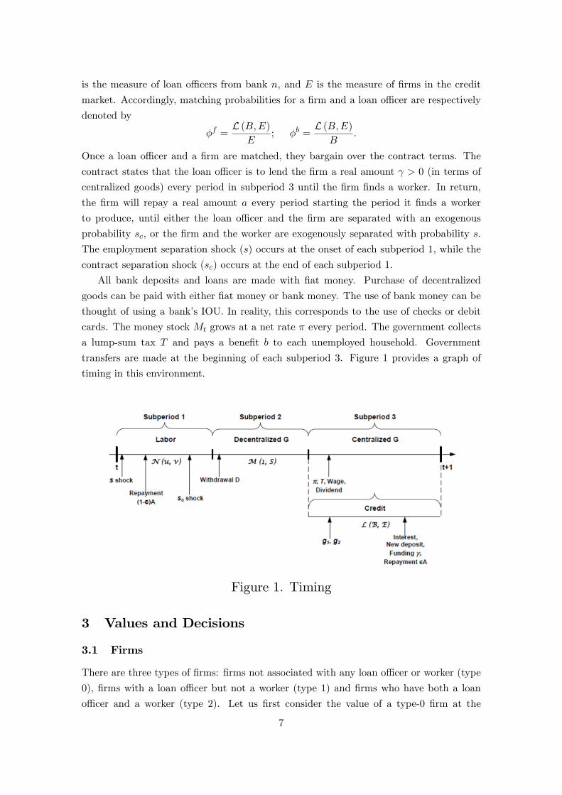
transfers are made at the beginning of each subperiod 3. Figure 1 provides a graph of

timing in this environment.

Figure 1. Timing

3 Values and Decisions

3.1 Firms

There are three types of firms: firms not associated with any loan offi cer or worker (type

0), firms with a loan offi cer but not a worker (type 1) and firms who have both a loan

offi cer and a worker (type 2). Let us first consider the value of a type-0 firm at the

7

beginning of subperiod 3 of t, represented by If0 . In the rest of the paper, we suppress

the time index t, and use a “hat”to denote period t+ 1 values. A type-0 firm can enter

the credit market at cost k > 0 to search for a loan offi cer for funding. The firm will be

matched with a loan offi cer with probability φf . Thus, the value of a type-0 firm at the

beginning of subperiod 3 is given by

If0 = max{0, φfβUf1 (a) + (1− φf )βIf0 − k}, (1)

where Uf1 (a) represents the value of a type-1 firm with a contract of repayment A (for

short, contract A) in t+ 1. If not matched, the firm remains a type-0 firm.

Now consider a type-1 firm with contract A at the beginning of subperiod 1 of t. This

firm is funded by the bank to recruit a worker. With probability λf , the firm finds a

worker and (after successfully negotiates wages) moves into subperiod 2 as a type-2 firm

of value V f2 (a). Otherwise, it remains a type-1 firm. Thus,

Uf1 (a) = λfV f2 (a) + (1− λf )βUf1 (a) . (2)

Next, consider a type-2 firm with contract A at the beginning of subperiod 2 with value

V f2 (a). First, a contract separation shock randomly hits such a firm. With probability sc,

the firm separates from the loan offi cer and will no longer repays the loan from that point

on. In this case, we simply use a = 0 to denote the status of a firm with a worker. Wage,

however, is not affected by this shock. With probability 1 − sc, the firm remains in the

loan contract. Next, the firm’s worker produces y units of goods. Then the decentralized

market starts, where the firm meets a household with probability αf . The two engage

in bargaining over (q, d). After the trade, the firm moves into the next subperiod with

y − c(q) units of real goods and a money balance of ρd, where ρ = 1/ (1 + π). If the firm

is not matched with a household, the firm moves into subperiod 3 with y units of real

goods and zero money balance. Thus,

V f2 (a) = sc

(αfW f

2 [y − c(q), ρd, 0] + (1− αf )W f2 (y, 0, 0)

)+ (1− sc)

(αfW f

2 [y − c(q), ρd, a] + (1− αf )W f2 (y, 0, a)

), (3)

where W f2 (·, ·, ·) is the value of a type-2 firm at the beginning of subperiod 3 of t. It is

given by

W f2 (x, z, a) = x+ z − w − a+ sβIf0 + (1− s)βV f

2 (a) , (4)

where x is the amount of inventory and z is the real money balance. In subperiod 3, this

firm pays wage w and make loan repayment a. Any remaining profit, x+z−w−a, will berebated in a lump sum to households as dividend. The employment relationship is subject

to a separation shock at the end of subperiod 3. With probability s, the relationship ends.

Then the firm becomes type-0 again and will participate in the credit market of period

8

t+ 1. Otherwise, the firm moves on still as a type-2.

3.2 Households

There are two types of households, employed and unemployed. First consider an employed

worker at the beginning of subperiod 3 of t with value W he (z), where z is the amount of

demand deposit (made in the previous period) due for principal and interests from the

bank in the current AD. Recall that demand deposit pays an interest and households can

use bank money to pay for goods. Thus, households will deposit all holdings of fiat money

in the bank as long as id > 0. The household’s value is given by

W he (z) = max

X,z{X + βUhe (z)} (5)

s.t. X + z = w + Π− T + (1 + id) z,

where z is the new demand deposit to be made in the current subperiod, Π is dividend

from firms, T is the lump-sum tax. Moreover, Uhe is the value of the household at the

beginning of subperiod 1 of t, and is given by

Uhe (z) = sV hu (z) + (1− s)V h

e (z) . (6)

The employment relationship gets hit by the separation shock with probability s. If so,

the worker becomes unemployed and continues with value V hu . Otherwise, she continues

as an employed worker with value V he . Then in the decentralized market, the household

purchases from a firm with probability αh, where she pays a real balance d for q units of

goods. That is,

V he (z) = αh[u (q) +W h

e (ρz − ρd)] + (1− αh)W he (ρz) . (7)

Similarly, the values of an unemployed worker are given by the following:

W hu (z) = max

X,z{X + βUhu (z)} (8)

s.t. X + z = b+ Π− T + (1 + id) z.

Uhu (z) = λhV he (z) + (1− λh)V h

u (z) (9)

V hu (z) = αh[u (q) +W h

u (ρz − ρd)] + (1− αh)W hu (ρz) . (10)

In the above, the unemployed worker finds a firm to work for with probability λh in

subperiod 1. Moreover, b is the unemployment insurance.

9

3.3 Banks

Banks n = 1, 2, · · · , N issue demand deposits to households in each subperiod 3. The

demand deposit is a contract between a bank and a household, defined as follows.

Definition 1 The demand deposit contract is written in subperiod 3 of period t. It statesthat: (i) the household is to deposit z in the bank by the end of t and is free to withdraw

any amount less than or equal to z before subperiod 3 of t+ 1. (ii) The bank is to pay a

net interest rate of id on the household’s bank balance at the beginning of subperiod 3 of

t+ 1.

Consider any bank n in subperiod 3. The bank sends a measure Bn of type-0 loan

offi cers to the credit market. Sending a type-0 loan offi cer incurs a real cost κ > 0.

Bargaining will be analyzed later. Let A = {a : a ∈ [0,∞)} be the set of all possiblecontracts and a ∈ A represents a contract with a particular periodic repayment level a.Moreover, A represents the contract term negotiated by loan offi cers and firms in the

current credit market. Now define gi (a) as the PDF of the distribution of all type-i

contracts of the bank at the beginning of subperiod 3 of t, with i = 1, 2. That is, gni (a)

represents the measure of type-i contracts with repayment requirement a for bank n. Let

Kn be the bank’s savings at the beginning of subperiod 3 of t. Let Zn be the amount of

demand deposits to accept in the current credit market. Moreover, Dn ∈[0, Zn

]is the

expected amount of withdrawal in the decentralized goods market immediately coming

up. Finally, let B−n be the aggregate decisions of all banks other than bank n. That is,

B−n =N∑

n 6=k=1Bk.

The bank’s periodic profit is given by

Πbn = ρKn +

∫a∈A

agn2 (a) + (1− κd) Zn − κBn − (1 + id) ρZnD

−γ[∫

a∈Agn1 (a) +Bnφ

b(Bn, B−n, E

)]−Dn − Kn − κf , (11)

where κd ∈ (0, 1) is the variable cost of handling demand deposits. To cover costs over

the current subperiod 3 to the next one, the bank has its own savings ρKn, together

with incoming repayments∫a∈A agn2 (a) and new demand deposits being issued Zn. In

terms of banking costs, there are the cost of handling demand deposits κdZn, cost of

sending new loan offi cers to the credit market κBn, cost of funding new and existing loans

γ[∫a∈A gn1 (a) +Bnφ

b(Bn, B−n, E

)], cost of paying principal and interests on previous

demand deposits (1 + id) ρZnD, cost of meeting demand of withdrawals Dn, a fixed cost

κf . In addition, the bank will also choose a new amount of its own savings Kn to put

aside. Note that∫a∈A gni (a) is the stock of type-i contracts held by the bank. Moreover,

10

Bnφb(Bn, B−n, E

)is the measure of new type-1 contracts created in the current subperiod

3.

Taking(id, Dn, E,A, B−n

)as given, the bank chooses

(Bn, Zn, Kn

)to maximize the

present value of current and future profits:

Vn (gn1, gn2, ZnD,Kn) = maxBn,Zn,Kn

{Πbn + βVn

(gn1, gn2, ZnD, Kn

)}(12)

s.t.

[ρKn + Zn

+ε∫a∈A agn2 (a)

]≥ γ

[∫a∈A

gn1 (a) +Bnφb(Bn, B−n, E

)]+κBn + (1 + id) ρZnD + κf (13)

Kn ≥ 0 (14)

ZnD = Zn −Dn (15)

gn1 (a) =

(1− λf

) [gn1 (a) +Bnφ

b(Bn, B−n, E

)],

if a = A(1− λf

)gn1 (a) , if a 6= A

(16)

gn2 (a) =

(1− sc) (1− s) gn2 (a)

+λf[gn1 (a) +Bnφ

b(Bn, B−n, E

)], if a = A

(1− sc) (1− s) gn2 (a) + λfgn1 (a) , if a 6= A.

(17)

Note that only a fraction ε ∈ [0, 1] of the repayments are received by the bank in AD of t.

Condition (13) is the liquidity constraint faced by the bank by the end of t. There

are costs that must be covered by this time. They are cost of lending associated with

κ and γ, payment of principal and interests on previous demand deposits, and the fixed

cost. What causes the liquidity constraint is that only a fraction ε ∈ [0, 1] of the loan

repayments are received by the bank by the end of t. Because of the delay in some of

the repayments, issuing new demand deposits and bank savings can both be helpful for

relieving the liquidity condition of the bank.

Condition (14) states that the bank’s savings must be nonnegative. Condition (15) is

the law of motion for the amount of demand deposit due at the beginning of subperiod 3.

The rest of the conditions in the bank’s decision problem are the laws of motion for the

distributions of contracts. At the beginning of subperiod 3 of t+ 1, the type-1 contracts

with particular requirement A consist of all of those previous and the newly-added type-1

contracts of A that are not matched with a worker in the immediately previous labor

market. Similarly, the evolution of type-2 contracts with A must include those existing

type-2 contracts that are not hit by a separation shock, and those newly added to the pool

of type-2. Finally, measures of the contracts with requirements other than the currently

offered term A evolve in their due courses given labor market shocks.

11

3.4 Bargaining solutions

3.4.1 The credit market

In the credit market, loan offi cers and firms engage in Nash bargaining. Let ηb be the

loan offi cer’s bargaining power against the firm and Vn1 (A) be the marginal value of a

type-1 contract to bank n. If the two parties agree on a deal, then the loan offi cer brings

the value Vn1 (A) back to the bank, and the firm receives βUf1 (A). If no deal, then the

bank receives nothing and the firm remains the value βIf0 . Therefore, bargaining solution

splits the surplus between the two parties according to

Vn1 (A)

β[Uf1 (A)− If0

] =ηb

1− ηb. (18)

3.4.2 The labor market

Firms and workers engage in Nash bargaining in the labor market. Effectively, the wage

rate w solvesV f2 (A)− Uf1 (A)

V he (z)− V h

u (z)=

ηf1− ηf

, (19)

where ηf is the firm’s bargaining power against the worker. If both parties agree, then

the firm receives V f2 (A) and the worker V h

e (z). Otherwise, the firm gets Uf1 (A) and the

worker V hu (z).

3.4.3 The decentralized goods market

In the decentralized goods market, matched firm and household bargain over the terms of

trade (q, d) according to the Kalai protocol. In particular, bargaining is to maximize the

surplus of the household subject to the condition that total trade surplus is split according

to the respective bargaining powers. Let µ be the bargaining power of a household. The

bargaining problem between a firm and a type i = e, u household is given by

max(q,d≤z)

{u(q) +W h

i (ρz − ρd)−W hi (ρz)

}(20)

s.t. u(q) +W hi (ρz − ρd)−W h

i (ρz) =µ

1− µ

{W f2 [y − c(q), ρd,A]−W f

2 (y, 0, A)}.

4 Equilibrium

Let the distributions of type-i contracts aggregated across all N banks be denoted by

gi (a) =N∑n=1

gni (a) , i = 1, 2.

Moreover, define g2 (0) as the measure of type-2 firms free of loan repayments. We have

the following definitions of equilibrium:

12

Definition 2 A symmetric banking equilibrium (Zn, Bn > 0) consists of values({Vn}Nn=1 ,

{Uhi , V

hi ,W

hi

}i=e,u

,{If0 , U

f1 , V

f2 ,W

f2

}),

decision rules({X, zi}i=e,u ,

{Bn, Zn, Kn

}Nn=1

), measures

(E, u, v, {Dn}Nn=1

), prices, terms

of trade and contract (w, q, d, id, A), and distributions {gi (a)}i=1,2 such that given policy(b, T, π), the following are satisfied:

1. All decisions are optimal;

2. All bargaining results are optimal in (18), (19) and (20);

3. Free entry of firms and banks is such that

If0 = 0 (21)

Πbn = 0, ∀ n; (22)

4. Matching in the labor markets satisfies:

N (u, v) = (1− u)s (23)

scg2 (A) = sg2 (0) ; (24)

5. All competitive markets clear. In particular, the clearing of money and demand

deposit market requires:

(1− u) ze + uzu +N∑n=1

Kn =M

P(25)

(1− u) ze + uzu =N∑n=1

Zn; (26)

6. Consistency: the distributions satisfy:

gi (a) =N∑n=1

gni (a) , i = 1, 2 and ∀a

where gni (a) obeys laws of motion (16)-(17);

7. Symmetry:(Bn, Zn, Kn

)are respectively the same for all n.

8. Government balances budget:

bu = T − πMP. (27)

13

Definition 3 A stationary equilibrium is one in which all real values and distributions

are time-invariant. In particular,

g1 (A) =

(1

λf− 1

)L (B,E) (28)

g2 (A) =L (B,E)

1− (1− sc) (1− s) (29)

gi (a) = 0 ∀ a 6= A ∈ A.

Equations (28)-(29) are derived from (16)-(17) given gni (A) = gni (A) for all n and i

in the steady state.

Lemma 1 In the steady state, the firm values are given by

Uf1 (A) =k

βφf=

λf

1− β(1− λf )V f2 (A) (30)

V f2 (A) =

y − w − (1− sc)A+ αf [ρd− c(q)] + sc (1− s)βV f2 (0)

1− β (1− sc) (1− s) (31)

V f2 (0) =

y − w + αf [ρd− c(q)]1− β (1− s) . (32)

Proof. These results are straightforward to derive given (21).

Lemma 2 The household choice of deposit balance z is independent of the current balancez. The functions W h

i (·) are linear with dW hi (z)/dz = 1+id for all z ∈ [0,∞) and i = e, u.

Proof. This is the classic Lagos-Wright result. It is straightforward from (5) and (8)

that

W he (z) = w + Π− T + (1 + id) z + max

z

{βUhe (z)− z

}(33)

W hu (z) = b+ Π− T + (1 + id) z + max

z

{βUhu (z)− z

}. (34)

Hence the lemma.

Proposition 1 The optimal bargaining solution in the decentralized goods market is thesame regardless of the type of the household. That is, for any i = e, u,

di (z) =

{z∗, if z ≥ z∗

z, if z < z∗

qi (z) =

{q∗, if z ≥ z∗

Ψ−1 (ρz) , if z < z∗.

14

Proof. Given (5), (8) and Lemma 2, we have for i = e, u,

W hi (ρz − ρd)−W h

i (ρz) = − (1 + id) ρd.

Then given (4), we have

W f2 [y − c(q), ρd]−W f

2 (y, 0) = ρd− c(q).

Together, the bargaining problem in (20) becomes the same for i = e, u and boils down

to

max(q,d≤z)

[u(q)− (1 + id) ρd] (35)

s.t. u(q)− (1 + id) ρd =µ

1− µ [ρd− c(q)] .

If the money constraint does not bind, i.e., d < z, then we can rearrange the bargaining

constraint to get

ρd =(1− µ)u(q) + µc(q)

(1− µ) (1 + id) + µ≡ Ψ (q) .

Then use the above to eliminate ρd in the objective of (35). The bargaining problem is

reduced to

maxq{u(q)− (1 + id) c(q)}

Therefore, the optimal choice of q solves

u′(q∗)

c′(q∗)= 1 + id. (36)

Accordingly, the optimal choice of payment z∗ is given by

ρz∗ = Ψ (q∗) . (37)

If the money constraint binds, i.e., d = z, then trade quantity can be directly solved from

the bargaining constraint. That is, q (z) = Ψ−1 (ρz) .

Proposition 2 In the steady state, household decisions are such that:(i) ze = zu;

(ii) If βρ (1 + id) < 1, then di (z) = z for i = e, u. Moreover, ze = zu = z in the

steady state, where z satisfies

αhu′(Ψ−1 (ρz)

)Ψ′ (ρz)

+(

1− αh)

(1 + id) =1

βρ. (38)

(iii) If βρ (1 + id) = 1, then di (z) < z for i = e, u. Moreover, ze = zu > z∗.

15

Proof. Let qi (·) and di (·) be the bargaining solutions in the decentralized goods market.Recall from (7) and (10) that

V hi (z) = αh[u (qi (z)) +W h

i (ρz − ρdi (z))] + (1− αh)W hi (ρz) , i = e, u.

Furthermore,

dUhe (z)

dz= s

dV hu (z)

dz+ (1− s)dV

he (z)

dz

= s[αh[u′ (qu (z)) q′u (z) + ρ (1 + id)

(1− d′u (z)

)] + (1− αh)ρ (1 + id)

]+ (1− s)

[αh[u′ (qe (z)) q′e (z) + ρ (1 + id)

(1− d′e (z)

)] + (1− αh)ρ (1 + id)

]= αh

{s [u′ (qu (z)) q′u (z)− ρ (1 + id) d

′u (z)]

+ (1− s) [u′ (qe (z)) q′e (z)− ρ (1 + id) d′e (z)]

}+ ρ (1 + id)

and

dUhu (z)

dz= λh

dV he (z)

dz+ (1− λh)

dV hu (z)

dz

= λh[αh[u′ (qe (z)) q′e (z) + ρ (1 + id)

(1− d′e (z)

)] + (1− αh)ρ (1 + id)

]+(

1− λh) [αh[u′ (qu (z)) q′u (z) + ρ (1 + id)

(1− d′u (z)

)] + (1− αh)ρ (1 + id)

]= αh

{λh [u′ (qe (z)) q′e (z)− ρ (1 + id) d

′e (z)]

+(1− λh

)[u′ (qu (z)) q′u (z)− ρ (1 + id) d

′u (z)]

}+ ρ (1 + id)

Finally, an interior optimal choice of zi from (5) and (8) requires

βdUhi (zi)

dz= 1, i = e, u. (39)

Therefore, households’steady-state money holdings, (ze, zu) are jointly solved from

1

β= αh

{s[u′ (qu) q′u (zu)− ρ (1 + id) d

′u (zu)

+ (1− s) [u′ (qe) q′e (ze)− ρ (1 + id) d′e (ze)

}+ ρ (1 + id) (40)

1

β= αh

{λh[u′ (qe) q′e (ze)− ρ (1 + id) d

′e (ze)]

+(1− λh

)[u′ (qu) q′u (zu)− ρ (1 + id) d

′u (zu)]

}+ ρ (1 + id) . (41)

The above implies

u′ (qu) q′u (zu)− ρ (1 + id) d′u (zu) = u′ (qe) q

′e (ze)− ρ (1 + id) d

′e (ze) . (42)

Immediately it follows that

ze = zu.

16

If the money constraint does not bind for the households, then we have q′i = d′i = 0.

Therefore,

βdUhi (zi)

dz= βρ (1 + id) .

But then the first-order condition (39) requires

βρ (1 + id) = 1.

Therefore, the money constraint must be binding for both types of households if βρ (1 + id) <

1. If this is the case, then (38) follows from (39). Obviously, if the money constraint does

not bind, then ze = zu > z∗.

In the steady state, per-capita divided from firms is given by

Π =[αf (ρd+ y − c(q)) + (1− αf )y − w −A

]g2 (A)

+[αf (ρd+ y − c(q)) + (1− αf )y − w

]g2 (0) . (43)

The two components in Π are respectively dividends from firms still making loan re-

payments and those without repayments. The measure of firms participating the labor

market is

v = g1 (A) + L (B,E) =L (B,E)

λf, (44)

given (28) and B = NBn. Moreover, in equilibrium total withdrawal faced by a bank is

given by

Dn =αhd (z)

N. (45)

Finally, we have the following results for the steady state:

L (B,E) = N (u, v)

λf =N (u, v)

v=L (B,E)

v

αf =M (1, g2 (A) + g2 (0))

g2 (A) + g2 (0)

αh = M (1, g2 (A) + g2 (0)) .

The first equation in the above is because in equilibrium, the inflow of type-1 firms (from

successful matching in the credit market) must be equal to the outflow of them (due to

successful matching in the labor market). Finally, let ξ be the Lagrangian multiplier for

the bank’s liquidity constraint (13).

4.0.4 Banking equilibrium

Theorem 4 If exists, the stationary banking equilibrium must have the money constraint

always binding for households in the decentralized goods market. In particular, the equi-

17

librium deposit rate id satisfies

βρ (1 + id) =1 + ξ − κd

1 + ξ. (46)

There may exist multiple equilibria of the following three types:

(i) ξ = Kn = 0. That is, the liquidity constraint does not bind for individual banks,

and that banks do not save. In this case, the steady state can be determined by solving

(B,E, u,N) from the following System I:

βφfλfV f2 (A)− k[1− β(1− λf )] = 0

L (B,E)− (1− u) s = 0

[φb (B,E) +B

N

∂φb

∂Bn][(1− λf )βV1 + λfβV2 − γ

]= κ

[(1− ρ (1 + id)) (1− αh)− κd]z +Ag2 (A)− γ[g1 (A) +Bφb (B,E)]− κB −Nκf = 0.

(ii) ξ > 0, Kn = 0. In this case, the steady state can be determined by solving

(B,E, u, ξ,N) from System II:

βφfλfV f2 (A)− k[1− β(1− λf )] = 0

L (B,E)− (1− u) s = 0

[φb (B,E) +B

N

∂φb

∂Bn][(1− λf )βV1 + λfβV2 − γ (1 + ξ)

]− κ (1 + ξ) = 0

[1− ρ (1 + id) (1− αh)]z + εAg2 (A)− γ[g1 (A) +Bφb (B,E)]− κB −Nκf = 0

(1− ε)Ag2 (A)− (αh + κd)z = 0.

(iii) ξ > 0, Kn > 0. In this case, the steady state can be determined by solving

(B,E, u, ξ,Kn, N) from System III:

βφfλfV f2 (A)− k[1− β(1− λf )] = 0

L (B,E)− (1− u) s = 0

[φb (B,E) +B

N

∂φb

∂Bn][(1− λf )βV1 + λfβV2 − γ (1 + ξ)

]− κ (1 + ξ) = 0

[1− ρ (1 + id) (1− αh)]z + ρNKn + εAg2 (A)− γ[g1 (A) +Bφb (B,E)]− κB −Nκf = 0

βρ (1 + ξ)− 1 = 0

(1− ε)Ag2 (A)− (αh + κd)z −NKn = 0.

In all of the above three cases, the contract term A solves

V1β[Uf1 (A)− If0

] =ηb

1− ηb, (47)

18

where

V2 =(1 + εξ)A

1− β (1− sc) (1− s) (48)

V1 =βλfV2 − γ (1 + ξ)

1− β(1− λf

) . (49)

Proof. Consider the decisions of individual bank n. The first-order condition for Zn > 0

is given by

1− κd + ξ + βV3 = 0. (50)

The first-order condition for Bn > 0 is[φb(Bn, B−n, E

)+Bn

∂φb

∂Bn

] [(1− λf

)βV1 + λfβV2 − γ (1 + ξ)

]= κ (1 + ξ) . (51)

The first-order condition for Kn is

βV4 − 1 ≤ 0, Kn ≥ 0. (52)

Moreover, the Envelope Theorem yields

V1 = −γ (1 + ξ) + β[(

1− λf)V1 + λf V2

](53)

V2 = A+ εAξ + β (1− sc) (1− s) V2 (54)

V3 = −ρ (1 + id) (1 + ξ) (55)

V4 = ρ (1 + ξ) (56)

Equations (50) and (55) imply

1− κd + ξ − βρ (1 + id) (1 + ξ) = 0.

Thus,

βρ (1 + id) =1 + ξ − κd

1 + ξ< 1 (57)

given κd > 0. Furthermore, (52) and (56) imply

βρ (1 + ξ)− 1 ≤ 0, Kn ≥ 0. (58)

Consider ξ = 0. Then the above yields

βρ (1 + ξ)− 1 = βρ− 1 < 0

given id > 0 and βρ (1 + id) < 1. Thus, ξ = 0 implies Kn = 0. That is, the bank does

not save as long as the liquidity constraint (13) does not bind.

19

Now consider Kn > 0. Then (58) yields

βρ (1 + ξ) = 1.

Combined with (57), we have1− κd + ξ

1 + id= 1.

Thus,

ξ = id + κd > 0.

That is, the liquidity constraint must be binding as long as the bank decide to save. Then

we have the following possible cases in equilibrium:

(i) ξ = 0, Kn = 0. In this case,

βρ (1 + id) = 1− κd.

We can solve for (B,E, u,N) from the following equations: free-entry of firms (21), la-

bor market matching condition (23), bank’s decision on Bn, (51), and bank’s zero-profit

condition.2

(ii) ξ > 0, Kn = 0. In this case, we can solve for (B,E, u, ξ,N) from the following

equations: (21), (23), (51), bank’s zero-profit condition, and (13) holding with equality.

(iii) ξ > 0, Kn > 0. In this case, we can solve for unknowns (B,E, u, ξ,Kn, N) from

the following equations: (21), (23), (51), bank’s zero-profit condition, and (13) and (58)

both holding with equality.

In all of the above cases, the loan repayment A is determined by (47).

4.0.5 Welfare

Welfare is defined as the weighted average of household values at the beginning of subpe-

riod 3. That is,

W1 = (1− u)[αhW h

e (z − d) +(

1− αh)W he (z)

]+ u

[αhW h

u (z − d) +(

1− αh)W hu (z)

]= (1− u)

[w + βUhe (z)

]+ uβUhu (z) + Π + idz − αh (1 + id) d− π

(z +NKn

), (59)

where the second equality is according to condition (27), Lemma 2 and Proposition 2. In

the above, Uhe (z) and Uhu (z) are given by

2Obviously the number of banks should be an integer. However, for analytical convenience, we solvefor N from the bank’s zero profit condition, which may not be an interger.

20

Uhu (z) =1

1− β

λh[w − b+ β

(1−λh−s)(w−b)1−β(1−λh−s)

]+ αhu (q)− z

+b (1− u) + Π− πMP + (1 + id) ρ(z − αhd)

Uhe (z) =

(1− s− λh

)(w − b)

1− β(1− s− λh

) + Uhu (z) .

In the above definition, households do not receive banking dividends. To analyze results

for the case where the number of banks N is taken as given, we also consider the definition

of welfare that households own banks and thus receive (nonnegative) banking dividends.

That is,

W2 =W1 + max [NΠbn, 0] . (60)

In the case of free-entry of banks, it does not matter which definition we use because

Πbn = 0.

5 Numerical Results

We conduct numerical exercises to obtain further results. We adopt the following func-

tional forms:

u (q) = ςuq1−σu

1− σuc (q) = ςcq

θ

L (B,E) = ωLB1−χLEχL

N (u, v) = ωNu1−χN vχN

M (1, S) = ωGSχG .

Moreover, the parameter values are listed in Table 1. For baseline computation, we set

policy variables as π = 0.02 and b = 0.5w, where w is the equilibrium wage. Moreover,

to highlight the effects of liquidity constraint, we set ε = 0. We summarize our numerical

results into two categories: one set of results are obtained taking the number of banks N

as given. That is, we solve the three systems listed in Theorem 4 without the competitive

banking condition Πbn = 0. For the second set of results, we endogenize N through the

competitive banking condition. That is, we solve the exact three systems as listed in

Theorem 4.

5.1 Equilibrium with N fixed

In this section, we assume that the number of banks is exogenously given and analyze

the equilibrium without entry or exit of banks. This is helpful for better understanding

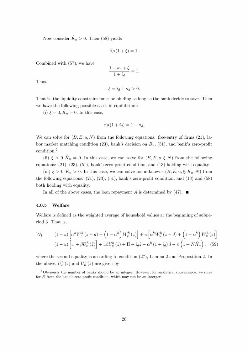
the equilibrium with entry, whose results will be presented in the next section. Figure 2

depicts how an individual bank’s profit varies with the number of banks in the economy,

21

i.e., Πbn (N). Panel A provides an overview of the curve for N ≥ 1 and Panel B is a

partial view of the function given N ≥ 6. The partial view is meant to provide a better

view of the segment where the equilibrium switches types as N changes. The red color

represents type I equilibria mentioned in Theorem 4, i.e., equilibria with ξ = Kn = 0.

The yellow color represents type II equilibria with ξ > 0 and Kn = 0. The green color

represents type III equilibria with ξ, Kn > 0. As is shown in Figure 2, bank profit first

deceases, then increases and finally decreases again as N rises. Moreover, the banking

equilibrium is of type I for lower N , type II for intermediate levels of N , and type III for

higher N .

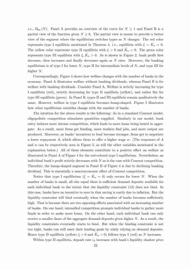
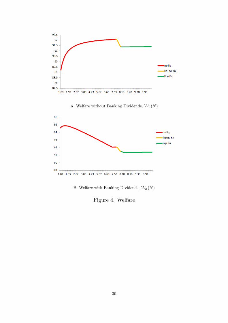
Correspondingly, Figure 4 shows how welfare changes with the number of banks in the

economy. Panel A illustrates welfare without banking dividends, whereas Panel B is for

welfare with banking dividends. Consider Panel A. Welfare is strictly increasing for type

I equilibria (red), strictly decreasing for type II equilibria (yellow), and rather flat for

type III equilibria (green). In Panel B, types II and III equilibria remain qualitatively the

same. However, welfare in type I equilibria becomes hump-shaped. Figure 5 illustrates

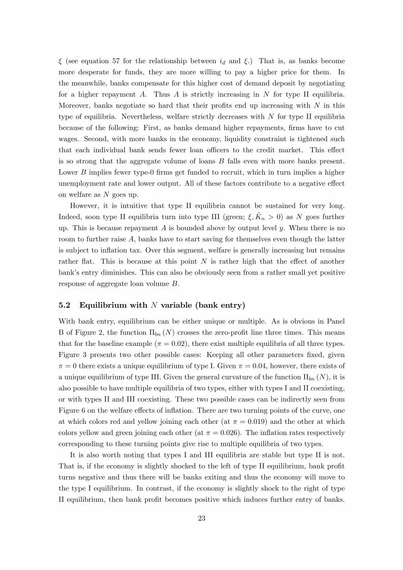
how other equilibrium variables change with the number of banks.

The intuition for the above results is the following: As in a standard Cournot model,

oligopolistic competition stimulates quantities supplied. Similarly in our model, bank

entry induces more intense competition, which leads to more loans being issued in aggre-

gate. As a result, more firms get funding, more workers find jobs, and more output are

produced. Moreover, as banks’incentives to lend become stronger, firms get to negotiate

a lower repayment A, which allows them to offer a higher wage w. (The responses of A

and w can be respectively seen in Figure 5, as will the other variables mentioned in the

explanation below.) All of these elements contribute to a positive effect on welfare as

illustrated in Panel A of Figure 4 for the red-colored type I equilibrium. Nevertheless, an

individual bank’s profit strictly decreases with N as is the case with Cournot competition.

Therefore, the hump-shaped segment in Panel B of Figure 4 is due to declining banking

dividend. This is essentially a macroeconomic effect of Cournot competition.

Notice that type I equilibrium (ξ = Kn = 0) only occurs for lower N . When the

number of banks is small, all else equal there is suffi cient demand deposits available for

each individual bank to the extent that the liquidity constraint (13) does not bind. In

this case, banks have no incentive to save in that saving is costly due to inflation. But the

liquidity constraint will bind eventually when the number of banks becomes suffi ciently

high. That is because there are two opposing effects associated with an increasing number

of banks. On one hand, intensified competition prompts individual banks to gather more

funds in order to make more loans. On the other hand, each individual bank can only

receive a smaller share of the aggregate demand deposits given higher N . As a result, the

liquidity constraints eventually starts to bind. But when the binding constraint is not

too tight, banks can still meet their lending goals by solely relying on demand deposits.

Hence type II equilibria (yellow; ξ > 0 and Kn = 0) follows type I (red) as N increases.

Within type II equilibria, deposit rate id increases with bank’s liquidity shadow price

22

ξ (see equation 57 for the relationship between id and ξ.) That is, as banks become

more desperate for funds, they are more willing to pay a higher price for them. In

the meanwhile, banks compensate for this higher cost of demand deposit by negotiating

for a higher repayment A. Thus A is strictly increasing in N for type II equilibria.

Moreover, banks negotiate so hard that their profits end up increasing with N in this

type of equilibria. Nevertheless, welfare strictly decreases with N for type II equilibria

because of the following: First, as banks demand higher repayments, firms have to cut

wages. Second, with more banks in the economy, liquidity constraint is tightened such

that each individual bank sends fewer loan offi cers to the credit market. This effect

is so strong that the aggregate volume of loans B falls even with more banks present.

Lower B implies fewer type-0 firms get funded to recruit, which in turn implies a higher

unemployment rate and lower output. All of these factors contribute to a negative effect

on welfare as N goes up.

However, it is intuitive that type II equilibria cannot be sustained for very long.

Indeed, soon type II equilibria turn into type III (green; ξ, Kn > 0) as N goes further

up. This is because repayment A is bounded above by output level y. When there is no

room to further raise A, banks have to start saving for themselves even though the latter

is subject to inflation tax. Over this segment, welfare is generally increasing but remains

rather flat. This is because at this point N is rather high that the effect of another

bank’s entry diminishes. This can also be obviously seen from a rather small yet positive

response of aggregate loan volume B.

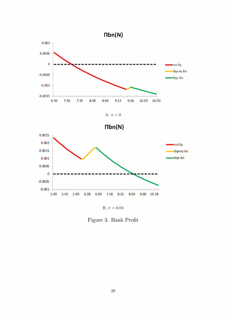
5.2 Equilibrium with N variable (bank entry)

With bank entry, equilibrium can be either unique or multiple. As is obvious in Panel

B of Figure 2, the function Πbn (N) crosses the zero-profit line three times. This means

that for the baseline example (π = 0.02), there exist multiple equilibria of all three types.

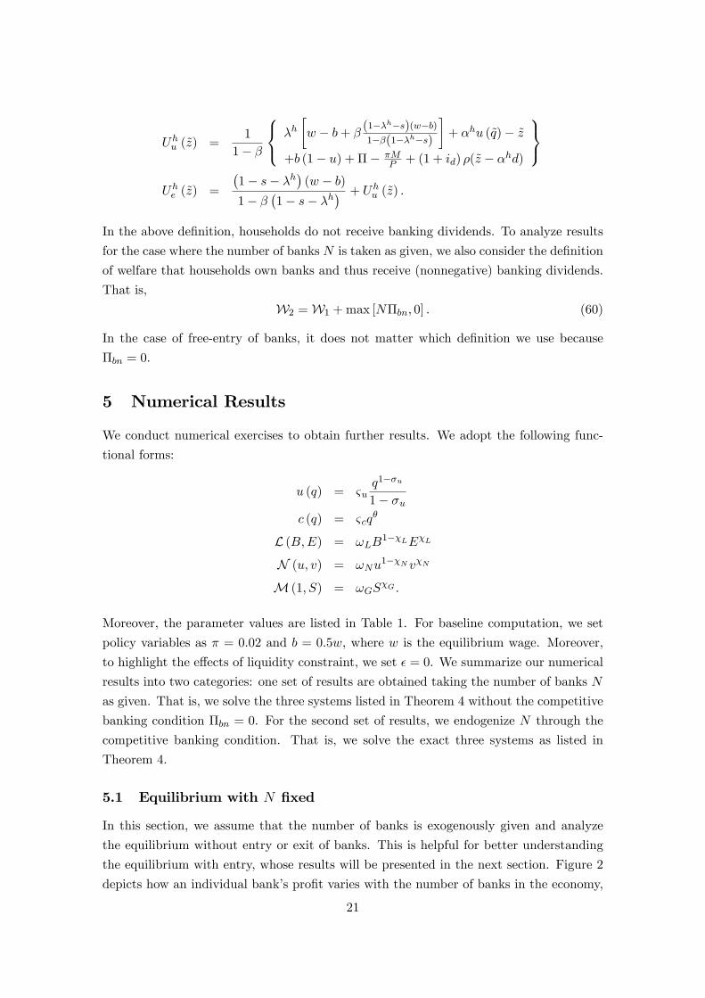
Figure 3 presents two other possible cases: Keeping all other parameters fixed, given

π = 0 there exists a unique equilibrium of type I. Given π = 0.04, however, there exists of

a unique equilibrium of type III. Given the general curvature of the function Πbn (N), it is

also possible to have multiple equilibria of two types, either with types I and II coexisting,

or with types II and III coexisting. These two possible cases can be indirectly seen from

Figure 6 on the welfare effects of inflation. There are two turning points of the curve, one

at which colors red and yellow joining each other (at π = 0.019) and the other at which

colors yellow and green joining each other (at π = 0.026). The inflation rates respectively

corresponding to these turning points give rise to multiple equilibria of two types.

It is also worth noting that types I and III equilibria are stable but type II is not.

That is, if the economy is slightly shocked to the left of type II equilibrium, bank profit

turns negative and thus there will be banks exiting and thus the economy will move to

the type I equilibrium. In contrast, if the economy is slightly shock to the right of type

II equilibrium, then bank profit becomes positive which induces further entry of banks.

23

Hence the economy will move toward type III equilibrium. With similar arguments, both

types I and III equilibria are stable.

It is clearly shown in Figure 4 that type I equilibria Pareto dominate, type II ranks

second and type III is Pareto inferior.

5.3 Welfare effects of inflation

Figure 6 depicts the equilibrium effects of inflation. First, inflation generally decreases

welfare regardless of the type of equilibrium. First of all, it is well known that inflation

has a negative effect on welfare because it depreciates the real value of money. Moreover,

in our model, ceteris paribus inflation worsens a bank’s liquidity condition. It is obvious

from Figure 6 that inflation strictly increases the deposit rate. The intuition is that, as

the real value of money declines, banks compete more intensely for funds by raising the

deposit rate they pay. This naturally tightens banks’liquidity constraint. In fact, it is

straightforward to see from (46) that id and ξ are positively related. As a result, the

higher the inflation rate, the more likely that banks become liquidity constrained, and

thus the lower the welfare.

Second, inflation can change the nature of the equilibrium. In particular, low inflation

(π < 0.019 in our example) only promotes type I equilibrium (red; stable and good),

whereas high inflation π > 0.026 only cultivates type III (green; stable yet bad). The

intermediate levels of inflation (0.019 ≤ π ≤ 0.026), however, can give rise to multiple

equilibria of all three types. Again, the reason is that inflation tightens up banks’liquidity

conditions. Figure 7 illustrates how bank profit and repayment level A vary with the

number of banks for given levels of inflation. As is shown in Figure 7, higher inflation

makes bank liquidity constraint start binding at a lower given number of banks. That

is, the red section of the bank profit curve is the shortest at π = 0.03. Moreover, both

the yellow and the green sections of the bank profit curve shifts up given higher inflation.

Due to the curvature of the bank profit function, the unique good equilibrium is more

likely to occur at lower inflation rates, the unique bad equilibrium tends to take place at

higher inflation rates, whereas all three types can occur at medium levels of inflation.

6 Conclusion

We have constructed a tractable macroeconomic model of banking to study the behavior

and economic impact of oligopolistic banks. Our model has three key features: (i) banks

as oligopolists; (ii) liquidity constraint for banks that arises simply from timing mismatch

of cashflows; and (iii) frictions in credit, labor and goods markets. We found that: First,

both the individual bank profit and welfare react non-monotonically to the number of

banks in equilibrium. Cournot-type of competition among banks does not always improve

welfare. On one hand, each bank needs to raise more funds for lending as having more

banks in competition stimulates bank lending. On the other hand, each bank only receives

24

a smaller share of the aggregate demand deposits given more banks in presence. When

the number of banks is suffi ciently high, banks become liquidity constrained and thus

welfare is dampened. Second, with entry to the banking sector, there may exist multiple

equilibria of three types: one is stable and Pareto dominates, another is unstable and

ranks second in welfare, and the third is stable yet Pareto inferior. Finally, the economy

tends to be in a unique good (as in Pareto dominant) equilibrium given low inflation, but

in a unique bad (Pareto inferior) equilibrium given high inflation. Intermediate levels of

inflation can induce equilibria of all three types.

References

[1] Berentsen A., G. Camera and C. Waller, 2007. "Money, Credit and Banking," Journal

of Economic Theory 135, 171-195.

[2] Cavalcanti, R. and N. Wallace, 1999. “Inside and outside money as alternative media

of exchange,”Journal of Money, Credit, and Banking (August), 443-457.

[3] Freixas, X. and J.C. ROCHET, 2008. "Microeconomics of Banking", Cambridge:

MIT Press.

[4] Gertler, M. and N. Kiyotaki, 2010. "Financial Intermediation and Credit Policy in

Business Cycle Analysis," in Handbook of Monetary Economics, Volume 3A, Ams-

terdam: Elsevier.

[5] Gertler, M. and N. Kiyotaki, 2015. "Banking, Liquidity and Bank Runs in an Infinite

Horizon Economy" American Economic Review 105(7), 2011-2043.

[6] Gertler, M., N. Kiyotaki and A. Prestipino, 2016. "Wholesale Banking and Bank

Runs in Macroeconomic Modelling of Financial Crises," NBERWorking Paper 21892.

[7] Gorton G., A. Winton, 2003. "Financial Intermediation," Handbook of the Economics

of Finance, Volume 1, Part A, Corporate Finance, 431-552.

[8] Gu C., Mattesini F., Monnet C., Wright R., "Banking: a New Monetarist Approach"

Review of Economic Studies 80(2), 636-66. 2013

[9] He, P., L. Huang and R. Wright, 2005. “Money and Banking in Search Equilibrium,”

International Economic Review 46, 637-70.

[10] He, P., L. Huang and R. Wright, 2008. “Money, Banking and Monetary Policy,”

Journal of Monetary Economics 55, 1013-1024.

[11] Lagos, R. and R. Wright, 2005. “A Unified Framework for Monetary Theory and

Policy Analysis,”Journal of Policitical Economy 113(3), 463-484.

[12] Sun, H., 2007. “Aggregate Uncertainty, Money and Banking,”Journal of Monetary

Economics 54(7), 1929-1948.25

[13] Sun, H., 2011. “Money, Markets and Dynamic Credit,”Macroeconomic Dynamics

15(S1), 42-61.

[14] Wasmer, E. and P. Weil, 2004. “The Macroeconomics of Credit and Labor Market

Imperfections,”American Economic Review 94(4), 944-963.

[15] Williamson, S., 2004. “Limited participation, private money, and credit in a spatial

model of money,”Economic Theory 24, 857-875.

[16] Williamson, S. and R. Wright, 2010a. “New Monetarist Economics: Models,”Hand-

book of Monetary Economics, Second Edition, forthcoming.

[17] Williamson, S. and R. Wright, 2010b. “New Monetarist Economics: Methods,”Fed-

eral Reserve Bank of St. Louis Review, forthcoming.

26

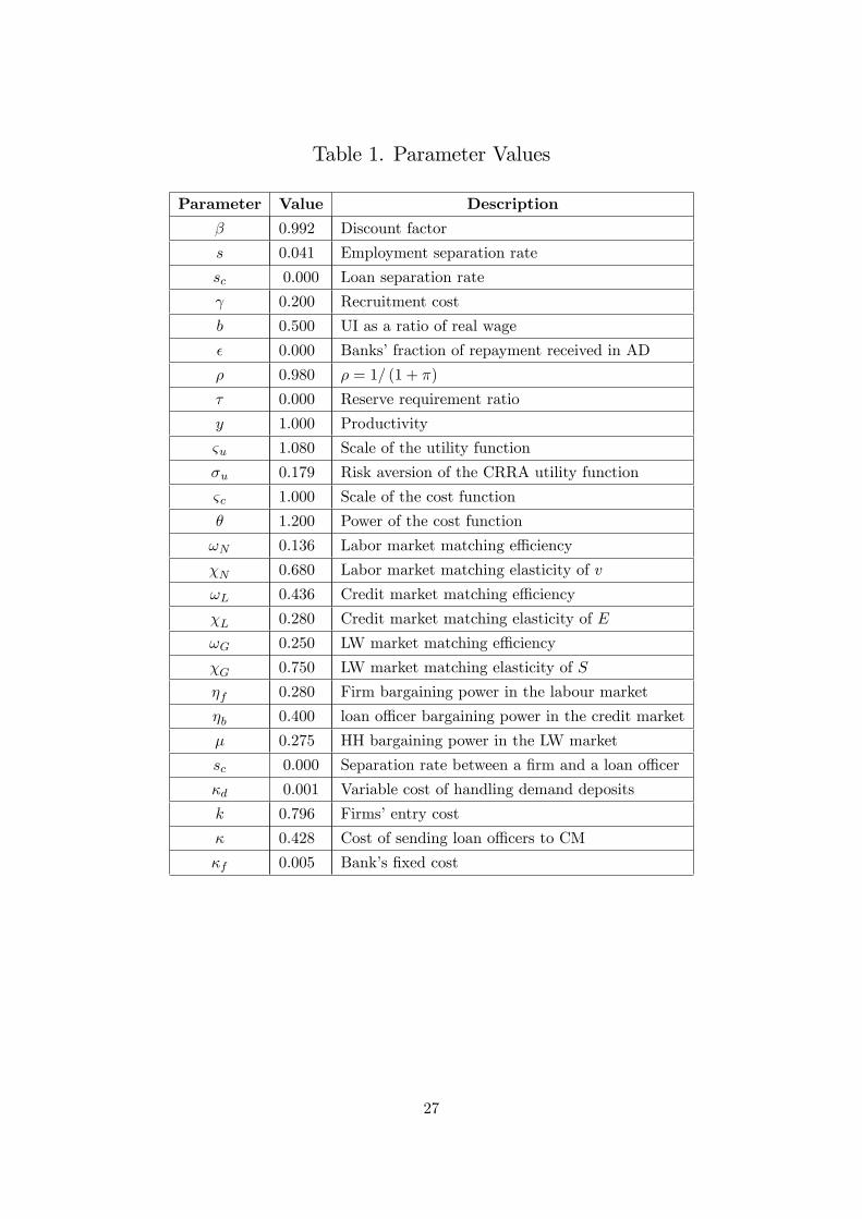
Table 1. Parameter Values

Parameter Value Description

β 0.992 Discount factor

s 0.041 Employment separation rate

sc 0.000 Loan separation rate

γ 0.200 Recruitment cost

b 0.500 UI as a ratio of real wage

ε 0.000 Banks’fraction of repayment received in AD

ρ 0.980 ρ = 1/ (1 + π)

τ 0.000 Reserve requirement ratio

y 1.000 Productivity

ςu 1.080 Scale of the utility function

σu 0.179 Risk aversion of the CRRA utility function

ςc 1.000 Scale of the cost function

θ 1.200 Power of the cost function

ωN 0.136 Labor market matching effi ciency

χN 0.680 Labor market matching elasticity of v

ωL 0.436 Credit market matching effi ciency

χL 0.280 Credit market matching elasticity of E

ωG 0.250 LW market matching effi ciency

χG 0.750 LW market matching elasticity of S

ηf 0.280 Firm bargaining power in the labour market

ηb 0.400 loan offi cer bargaining power in the credit market

µ 0.275 HH bargaining power in the LW market

sc 0.000 Separation rate between a firm and a loan offi cer

κd 0.001 Variable cost of handling demand deposits

k 0.796 Firms’entry cost

κ 0.428 Cost of sending loan offi cers to CM

κf 0.005 Bank’s fixed cost

27

A. Overview (N ≥ 1)

B. Partial View (N ≥ 6)

Figure 2. Bank Profit (π = 0.02)

28

A. π = 0

B. π = 0.04

Figure 3. Bank Profit

29

A. Welfare without Banking Dividends, W1 (N)

B. Welfare with Banking Dividends, W2 (N)

Figure 4. Welfare

30

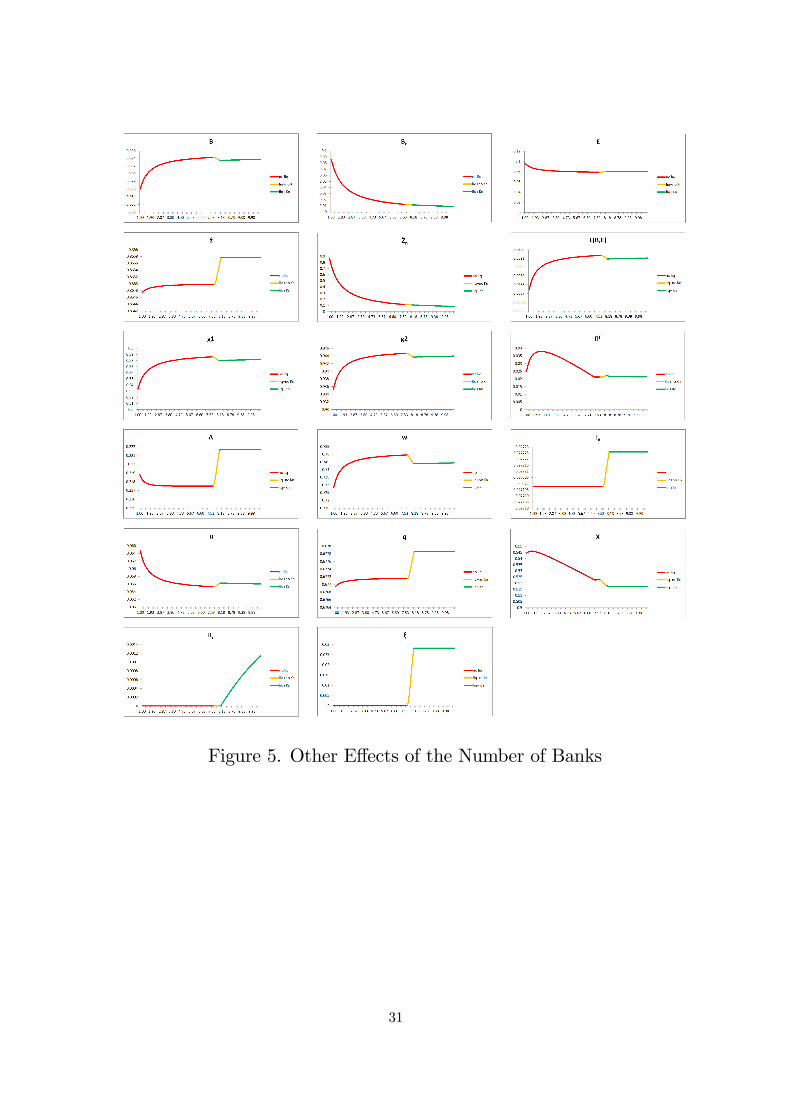
Figure 5. Other Effects of the Number of Banks

31

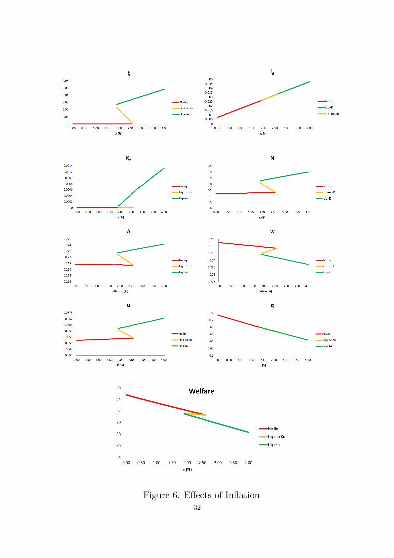
Figure 6. Effects of Inflation32

Figure 7. Inflation, Bank Profit and the Number of Banks

33