Universidade de Brasília

Instituto de Ciências Biológicas

Programa de Pós Graduação em Ecologia

A importância do tempo noestudo de peixes recifais:

métodos, interações ecomunidades

Gabriel Santos Garcia

Brasília - DF

Fevereiro de 2021

Universidade de Brasília

Instituto de Ciências Biológicas

Programa de Pós Graduação em Ecologia

Dissertação de Mestrado

A importância do tempo no estudo depeixes recifais: métodos, interações e

comunidades

Gabriel Santos Garcia

Orientador

Murilo Sversut DiasUniversidade de Brasília

Coorientador

Guilherme Ortigara LongoUniversidade Federal do Rio Grande do Norte

Dissertação de Mestrado apresentada ao Programade Pós Graduação em Ecologia da Universidadede Brasília como requesito para obtenção do títulode Mestre em Ecologia

Brasília, DF25 de Fevereiro de 2021

Gabriel Santos GarciaDissertação de Mestrado

A importância do tempo no estudo de peixes recifais:Métodos, Interações e Comunidades

Banca examinadora

Murilo Sversut DiasPresidente/Orientador

UnB

Guilherme Ortigara LongoCoorientador

UFRN

Ronaldo Bastos Francini-FilhoMembro examinador externo

CEBIMar - USP

Guarino Rinaldi ColliMembro examinador interno

UnB

Eduardo Bessa Pereira da SilvaMembro examinador suplente

UnB

25 de Fevereiro de 2021

3

“No que diz respeito à física, a flecha dotempo é apenas uma propriedade daentropia.”Arthur Eddington

"Diante da vastidão do tempo e daimensidão do universo, é um imenso prazerpara mim dividir um planeta e uma épocacom você."Carl Sagan

“São os mecanismos interligados einterativos de evolução e ecologia, cada umdos quais é ao mesmo tempo um produto eum processo, que são responsáveis pelavida como a vemos e como ela tem sido.“James Valentine

“Alegre-se com a vida, porque ela lhe dá achance de amar, trabalhar, brincar e olharpara as estrelas .“Henry van Dyke

4

Agradecimentos

Este trabalho foi feito a muitas mãos. Não cheguei até aqui sozinho e certamente não

vou continuar só. Portanto são muitas pessoas a agradecer.

Agradeço à minha família, cujo apoio foi o pilar que me estimulou a começar e

continuar a carreira acadêmica;

Ao CNPq, pela bolsa que permitiu a execução desse mestrado;

A todas e a todos que estiveram em campo juntando as informações que se

transformaram nessa dissertação, obrigado pelo esforço e dedicação;

À equipe do SISBIOTA-MAR, pela logística de coleta das informações que se

transformaram no terceiro capítulo desta dissertação;

Aos demais alunos do 11° e 12° Curso de Ecologia, Biogeografia e Ecolução de Peixes

Recifais pelo apoio na coleta de dados usados no segundo capítulo;

A toda a equipe do PELD-ILOC, por confiarem em mim para estudar mais de uma

década de trabalho intensivo;

Ao pessoal do Aquaripária, por tornarem o dia-a-dia, almoços e cafézinhos muito mais

alegres. Esses momentos de risadas fizeram toda a diferença na produtividade;

Aos amigos e também alunos do programa de Ecologia, pelas vivências, conversas e

boas risadas;

Ao pessoal do laboratório de ecologia marinha da UFRN, por estarem sempre

disponíveis a ajudar e conversar;

Aos amigos e amigas do Laboratório de Macroecologia e Biogeografia Aquática, pela

convivência em Brasília e depois, durante a pandemia;

Ao meu coorientador, Guilherme, pela ajuda, conversas e discussões na academia e fora

dela;

Ao meu orientador, Murilo, por ter me aturado durante dois anos. Obrigado por todas as

horas de ensino, conversa, discussões, rodadas e mais rodadas de revisões e pela

persistência em me aceitar como aluno, mesmo trabalhando com temas tão fora do seu

habitual. O apoio em Brasília e durante a quarentena foi fundamental para meu

desenvolvimento profissional e serei eternamente grato por isso;

A todos os contribuintes diretos e indiretos dessa dissertação,

Muito obrigado!

5

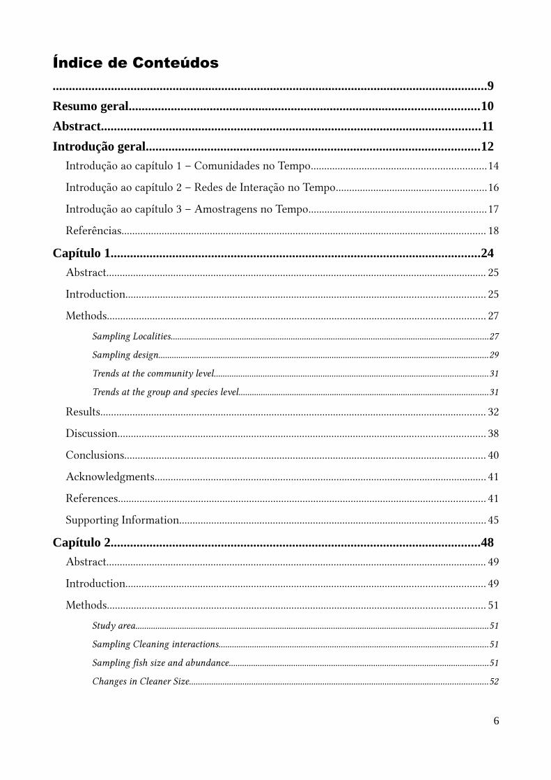
Índice de Conteúdos......................................................................................................................................9

Resumo geral............................................................................................................10

Abstract.....................................................................................................................11

Introdução geral.......................................................................................................12

Introdução ao capítulo 1 – Comunidades no Tempo.................................................................14

Introdução ao capítulo 2 – Redes de Interação no Tempo........................................................16

Introdução ao capítulo 3 – Amostragens no Tempo..................................................................17

Referências........................................................................................................................................ 18

Capítulo 1..................................................................................................................24

Abstract.............................................................................................................................................. 25

Introduction...................................................................................................................................... 25

Methods............................................................................................................................................. 27

Sampling Localities...............................................................................................................................................27

Sampling design....................................................................................................................................................29

Trends at the community level...........................................................................................................................31

Trends at the group and species level................................................................................................................31

Results................................................................................................................................................ 32

Discussion......................................................................................................................................... 38

Conclusions....................................................................................................................................... 40

Acknowledgments............................................................................................................................ 41

References......................................................................................................................................... 41

Supporting Information.................................................................................................................. 45

Capítulo 2..................................................................................................................48

Abstract.............................................................................................................................................. 49

Introduction...................................................................................................................................... 49

Methods............................................................................................................................................. 51

Study area...............................................................................................................................................................51

Sampling Cleaning interactions.........................................................................................................................51

Sampling fissh size and abundance.....................................................................................................................51

Changes in Cleaner Size......................................................................................................................................52

6

Species strength......................................................................................................................................................53

Species selectivity..................................................................................................................................................53

Results................................................................................................................................................ 54

Cleaning interactions............................................................................................................................................54

Changes in Cleaner Size......................................................................................................................................55

Species Strength.....................................................................................................................................................56

Cleaner selectivity.................................................................................................................................................57

Discussion......................................................................................................................................... 57

Effeect of intermitteent cleaners.............................................................................................................................57

Selectivity on cleaning..........................................................................................................................................58

Conclusions....................................................................................................................................... 59

Acknowledgments............................................................................................................................ 60

References......................................................................................................................................... 60

Supporting material......................................................................................................................... 63

Capítulo 3..................................................................................................................68

Abstract.............................................................................................................................................. 69

Introduction...................................................................................................................................... 69

Materials and Methods.................................................................................................................... 71

Sampling design and video analysis..................................................................................................................71

Statistical analysis of sampling time.................................................................................................................72

Statistical analysis of video number..................................................................................................................73

Cost-efficciency between observed time and number of videos......................................................................73

Results................................................................................................................................................ 75

Sampling Time.......................................................................................................................................................75

Number of Videos..................................................................................................................................................75

Cost-efficciency between number and length of videos...................................................................................77

Discussion......................................................................................................................................... 79

Acknowledgements.......................................................................................................................... 81

References......................................................................................................................................... 82

Supporting Information.................................................................................................................. 86

Conclusão geral........................................................................................................95

7

Índice de FigurasIntrodução geral.......................................................................................................12

Figura 1. Sítios amostrais no Atlântico Sudoeste abordados nesta dissertação.....................14

Figura 2. Isóbatas de 1000m, mostrando a plataforma continental nas regiões tropicais do globo................................................................................................................................................... 15

Capítulo 1..................................................................................................................24

Figure 1. Details on the location of monitored islands relative to the South American Coast and the sampling sites within each island........................................................................28

Figure 2. Changes in mean fissh composition through time summarized by non-metric multidimensional scalings (NMDS) with two axes.....................................................................34

Figure 3. Fluctuations in groups biomass through time.............................................................37

Figure 4. Net changes in fissh groups biomass observed in over ten years of monitoring in the four Brazilian oceanic islands................................................................................................. 38

Figure S1. Net changes in species biomass..................................................................................46

Figure S2. Trends in biomass of individual species, sorted by groups (lines) and Islands (columns)........................................................................................................................................... 47

Capítulo 2..................................................................................................................48

Figure 1. Location of Arraial do Cabo within South America, detailing sampling sites in the Forno Bay.................................................................................................................................... 52

Figure 2. Network of cleaning interactions recorded in 2019 and 2020.................................55

Figure 3. Species strength metric recorded in 2019, 2020 and combining both years..........57

Figure S1. Individual based accumulation on number of client species..................................63

Figure S2. Size distribution of facultative cleaners obtained form underwater visual censuses and the size distribution of cleaners engaging in cleaning interactions................64

Figure S3. Non-metric multidimensional scaling of visual censuses showing available predictors........................................................................................................................................... 65

Figure S4. Comparison of client selectivity by Elacatinus fisgaro and Pomacanthus paru...66

Capítulo 3..................................................................................................................68

Figure 1. Relationship between richness (top) and main species composition (bottoom) withnumber of videos (right) and their length (left)..........................................................................77

Figure 2. Trade offss between sampling more or sampling longer videos (above) and the efficciency in each combination of number of samples and video length (below)..................79

Figure S1. Map showing location of the fisve sampling sites relative to the coastline (grey area).................................................................................................................................................... 86

8

Figure S2. Residuals graphical analysis of linear mixed effsects model...................................89

Figure S3. Graphical residual analysis of linear models used to test trade-offss between video number and length for detecting richness and composition..........................................94

Conclusão geral........................................................................................................95

Figura 1. Resumo gráfisco do primeiro capítulo...........................................................................95

Figura 2. Resumo gráfisco do segundo capítulo...........................................................................96

Figura 3. Resumo gráfisco do terceiro capítulo.............................................................................98

Figura 4. Esquema resumindo o conteúdo dos três capítulos...................................................98

Índice de TabelasCapítulo 1..................................................................................................................24

Table 1. Thee effsect of assessed predictors on fissh assemblages at each oceanic Islands basedon a PERMANOVA......................................................................................................................... 33

Table 2. Pairwise comparisons of assemblage composition based on fissh biomass between four time periods.............................................................................................................................. 35

Capítulo 2..................................................................................................................48

Table S1. Parameters estimate derived from the PERMANOVA.............................................65

Table S2. Parameter estimates on the linear model....................................................................67

Capítulo 3..................................................................................................................68

Table 1. Summary of statistical procedures used to assess the effsects of time, videos and both predictors on species richness and composition................................................................74

Table S1. Details on physical parameters of each sampling localities....................................87

Table S2. Linear mixed model parameters estimates on richness explained by time...........88

Table S3. Parameters and statistics estimated for the PERMANOVA used to test the relation between species composition (similarity on species presence) and time (expressed by 1 minute time steps)................................................................................................................... 90

Table S4. Pairwise comparisons of composition between time steps (pairwise PERMANOVAs)............................................................................................................................... 91

Table S5. Break-Point estimates for richness and composition similarity and its respective confisdence intervals......................................................................................................................... 92

Table S6. Parameter estimates provided by the linear model relating minimum number of replicates (as breakpoints) and video length (in minutes).........................................................93

9

Resumo geral

Comunidades biológicas são dinâmicas e mudam constantemente no tempo. No entanto, abordagenstemporais costumam ser escassas e a maioria dos estudos na ecologia marinha brasileira usamamostragens em escalas de tempo curtas. Pensando nisso, nesta dissertação realizei três estudosfocados no tempo, usando as assembleias de peixes recifais do Atlântico Sudoeste como organismosmodelo.

No primeiro capítulo eu descrevi o histórico de mudanças das assembleias de peixes recifais emquatro ilhas oceânicas brasileiras usando mais de uma década de informações coletadas por umprograma de monitoramento a longo prazo (PELD-ILOC). As assembleias de peixes são variáveis,onde o tempo per se explica de 30% a 50% das mudanças na composição. Entretanto, essasmudanças não apresentam uma direção clara e parecem ser flutuações estocásticas provenientes dasoscilações populacionais de diferentes espécies. Além disso, cada ilha teve um histórico demudanças próprio que sugere a atuação de um mecanismo ecológico diferente em cada local, queincluem cenários estabilidade dinâmica, substituições de espécies intraguilda, cascatas tróficas edistúrbios provavelmente ligados a floração de macroalgas. Toda essa variabilidade fornece umindicativo das vantagens trazidas pelo acompanhamento a longo prazo.

No segundo capítulo, eu avaliei como interações de limpeza — uma relação mutualísticacaracterística de ambientes recifais, na qual uma espécie (limpador) remove parasitas, muco ou pelemorta de uma outra espécie (cliente) — variaram no período de dois anos em uma enseada deArraial do Cabo. As redes de interações dependem prioritariamente de um limpador especializado,Elacatinus figaro e de um facultativo, Pomacanthus paru, que atendem a conjuntos de espéciessemelhantes. Cardumes de juvenis de Haemulon também atuaram como limpadores facultativosquando juvenis, mas atendem principalmente a um cliente, Pseudupeneus maculatus. No entanto, oengajamento de Haemulon na interação variou entre anos, oferecendo uma oportunidade de limpezatemporária. Ainda assim, a maior parte das redes de interações se manteve semelhante entre os anosdevido à presença constante de E. figaro e P. paru. mostrando que se as espécies centrais foremmantidas, o restante da rede permanece estável.

Por fim, o objetivo do terceiro capítulo foi avaliar como amostragens de peixes por vídeos podem sebeneficiar ao incluir o tempo de gravação, buscando identificar estratégias de amostragem maiseficientes. O capítulo foca em dois tipos de amostragens: se ter mais réplicas com vídeos curtos oupoucos vídeos mais longos. Usando recifes da costa leste do Rio Grande do Norte como modelo,foi encontrado que a maioria das espécies é detectada nos primeiros minutos de filmagem, ondecinco vídeos de cinco minutos foram suficientes para detectar boa parte da riqueza de espécies doestado. Para atingir um mesmo número de espécies, tempo e réplicas podem ser intercambiáveis,mas essa relação não é linear, de modo que a taxa de detecção de novas espécies por minuto caidrasticamente quando a duração dos vídeos aumentou. Dessa forma, muitas réplicas de vídeos maiscurtos são mais eficientes por unidade de tempo que poucas réplicas de vídeos mais longos.

Nesta dissertação, eu espero ter demonstrado como a ecologia recifal brasileira pode se beneficiarao incluir o tempo para responder padrões, demonstrando que perspectivas temporais permitem umentendimento mais profundo dos mecanismos determinantes da estrutura das assembleias marinhasrecifais.

Palavras-Chave: Atlântico Sudoeste, Monitoramento, Ilhas Oceânicas, Limpeza, FilmagensRemotas Subaquáticas

10

Abstract

Biological communities are dynamic and changes constantly through time. Still, surveys within theBrazilian marine ecology counts on few temporal assessments. In an attempt to inspire the spreadof temporal perspectives in the field, in this dissertation I conducted three surveys using a temporalframework, taking the Southwestern Atlantic reef fishes as target organisms.

The first chapter goal was to describe how reef fish assemblages changed within the last decade infour Brazilian oceanic islands, using data recorded by a long-term monitoring program since 2007(PELD-ILOC). The fish assemblages rearranged constantly through time, with time itselfaccounting from a third to half the variability in species composition. However, those changes weremostly non-directional, likely resulting from random fluctuations on fish populations. Each islandhad their own set of changes, suggesting a distinct mechanism could explain changes in each island.Those ranged between a dynamic stability scenario to a within-group turnover, a trophic cascadeand a dusturbance-recover dynamics (probably linked to algal blooms). This diversity of processesshows how temporal perspectives can improve our current understanding about biologicalcommunities by suggesting new ideas on community functioning.

Beyond tracking changes of composition, time assesments may be useful to characterize othertopics within community ecology. Minding these applications, the second chapter attempted todescribe cleaning interactions — a mutualistic relation common in reefs in which a cleaner speciesremove parasites and dead skin from a client species — in a rocky reef in Southwestern Brazil usinga two years temporal perspective. The local cleaning networks rely mostly on two species,Elacatinus figaro and Pomacanthus paru. Schools of juvenile Haemulon also engaged as second-party cleaners, though attending mostly a single client (Pseudupeneus maculatus). Cleaningactivities of Haemulon species decreased substantially between years, such that their importance onthe 2020 network was almost negligible. The cleaning netoworks still changed little between years,such that as long as the central species E. figaro and P. paru remain on the reef, the cleaninginteraction shall remain stable.

The last chapter was dedicated to unravel how a time perspective could be applied to harvest fieldsamples. The main goal was to evaluate the trade-offs associated to methodological decisions inrecording fish richness and composition through remote filming. Particularly, the focus lied uponidentifying which strategy record more species under a smaller effort, if either using severalreplicates of short videos or a few replicates of longer videos. The analysis took place on reefs inNortheastern Brazil. Most of the local richness was detected within the video first minutes, suchthat as few as 5 videos lasting for as short as 5 min could reveal most of the local richness. Timeand replicates were interchangeable in order to reach a same species number, though this relationwas non-linear, such that new records per minute dropped quickly towards longer videos. So, usingshorter videos provide a more efficient way to record more species within less sampling time.

By exploring these distinct issues, I expect to have shown how community ecology on reef systemswould benefit from including a temporal perspective, allowing for a deeper understanding about themechanisms regulating the structure of marine reef communities.

Keywords: Southwestern Atlantic; Monitoring; Oceanic Islands; Cleaning Interactions; RemoteUnderwater Videos

11

Introdução geral

Comunidades biológicas são dinâmicas e podem ser estudadas em várias escalas

de tempo (MURPHY et al., 1988; OTTERSEN et al., 2010). Estudos envolvendo

variação temporal costumam ser escassos, mas permitem um entendimento mais profundo das

espécies e de como elas interagem entre si e com o ambiente (MAGURRAN et al., 2010). Uma

mesma comunidade pode ser acompanhada por minutos, meses ou anos e revelar diferentes facetas

da sua estrutura e funcionamento em cada tempo. Abordagens na escala de dias e semanas mostram

um recorte instantâneo das comunidades, que costumam ser úteis para descrever a composição de

espécies e como elas interagem entre si e com o ambiente (AUED et al., 2018; FONTOURA et al.,

2020; MORAIS; FERREIRA; FLOETER, 2017; QUIMBAYO et al., 2018). Na escala de anos ou

décadas, temos mais detalhes sobre o caminho que as comunidades tomaram recentemente para

chegar em seu estado atual, trazendo um conhecimento mais detalhado sobre sua estabilidade no

tempo (BATES et al., 2014; KELMO; ATTRILL, 2013; WOLFF; RUIZ; TAYLOR, 2012).

Estudos com comunidades biológicas possuem escalas temporais bem variadas,

de alguns dias até milhões de anos (BONTHOUX; BALENT, 2012; CONDAMINE;

ROLLAND; MORLON, 2013). Por exemplo, as filogenias de comunidades acompanham o

histórico evolutivo das espécies, detalhando quais processos geológicos e biogeográficos moldaram

a composição local no tempo geológico (NARWANI et al., 2015). Por outro lado, as comunidades

também podem ser descritas usando janelas de tempo curtas, de apenas alguns dias ou semanas, que

permitem realizar inferências ecológicas ao custo de assumir que as comunidades são estáticas

(AUED et al., 2018; FONTOURA et al., 2020; LONGO et al., 2019; MORAIS; FERREIRA;

FLOETER, 2017). Na prática, as comunidades biológicas dificilmente permanecem constantes no

tempo porque as espécies são dinâmicas, sofrendo flutuações populacionais em resposta às

mudanças de outras espécies ou mesmo das condições ambientais.

O ambiente está sempre suscetível a sofrer alterações, sejam elas graduais, como

as mudanças no clima (CONDAMINE; ROLLAND; MORLON, 2013), ou abruptas

(também chamados de distúrbios), como em tempestades ou incêndios florestais (BURKLE et al.,

2019; DUFOUR et al., 2019; REAGAN, 1991). Os distúrbios garantem que as comunidades sejam

dinâmicas ao provocar mortalidade de indivíduos, seja ela seletiva ou não, abrindo oportunidades

para que outras espécies aumentem em abundância (COLLINS, 2000). Os impactos da perda de

indivíduos podem ser instantâneos ou persistir ao longo do tempo, impedindo que as comunidades

se aproximem de um equilíbrio (JACQUET; ALTERMATT, 2020). Acompanhar as comunidades no

tempo consiste em uma das melhores estratégia para entender os efeitos imediatos e tardios dos

distúrbios (MAGURRAN et al., 2010). As mudanças demográficas, como nascimento e mortalidade

Escalas de tempo

Por que monitorar?

Comunidades no tempo5

10

15

20

25

30

35

costumam ser mais aparentes e por isso são o alvo da maioria dos estudos de monitoramento

(MAGURRAN et al., 2010).

Amostrar comunidades periodicamente demanda esforços e recursos que

frequentemente não estão à disposição, tornando abordagens a longo prazo mais raras,

especialmente nos trópicos (MAGURRAN et al., 2010). Métodos indiretos podem ser usado para

extrair dados com relevância biológica a exemplo do acervo fossilífero e de amostragens de gases

atmosféricos em núcleos de gelo (CHEVALIER et al., 2020; STOLPER et al., 2016), mas acabam

não fornecendo dados tão precisos quanto os obtidos pela amostragem direta. Assim, para suprir a

demanda de informações temporais, redes de monitoramento foram estabelecidas em várias

paisagens naturais em especial nas nações desenvolvidas do hemisfério norte, com intuito de

mostrar qual o estado atual da biota nesses sítios e suas mudanças ao longo do tempo

(MAGURRAN et al., 2010; PROENÇA et al., 2017).

Uma boa parte do conhecimento existente sobre o impacto dos distúrbios

climáticos e humanos veio de programas de monitoramento de longo prazo. Por

exemplo, as redes de monitoramento de recifes de corais do Caribe, Índico e Pacifico mostraram um

padrão recorrente de mudanças nas últimas décadas, perdendo cobertura de corais em resposta a

ondas de calor (HUGHES et al., 2018). Ao mesmo tempo, o monitoramento revelou que a

sobrepesca e a mortalidade em massa de corais afetaram essas comunidades em diferentes escalas

de tempo, trazendo efeitos imediatos e tardios (KEITH et al., 2018; STUART-SMITH et al., 2018;

SULLY et al., 2019). A longo prazo, a sobrepesca gradualmente remove predadores de topo, o que

reestrutura as comunidades locais e muda suas interações tróficas em poucas décadas (PADDACK

et al., 2009). Já as ondas de calor causam perda de cobertura de corais, alterando a fisionomia

dessas comunidades em poucos dias, mas com impactos na complexidade estrutural dos recifes que

duram anos (ALVAREZ-FILIP et al., 2009).

Tendo em vista o efeito que o tempo tem sobre as comunidades biológicas,

meu objetivo foi avaliar comunidades recifais sob uma perspectiva temporal, usando peixes como

organismos modelo. Essa escolha foi baseada na facilidade de amostragem, diversidade de

interações e riqueza relativamente alta de espécies (PARRAVICINI et al., 2013). Serão três

abordagens, cada uma em um capítulo, explorando como o tempo afeta a amostragem, o modo

como as espécies interagem e a estrutura das comunidades. Todas ocorreram em recifes rasos no

Atlântico sudoeste (Figura 1). Cerca de 730 espécies de peixes são associadas a recifes nessa

província, das quais 405 são exclusivamente recifais e 102 são endêmicas (PINHEIRO et al., 2018).

13

Redes de monitoramento

Custo vs vantagens

Grupo alvo

40

45

50

55

60

65

Figura 1. Sítios amostrais no Atlântico Sudoeste abordados nesta dissertação. O primeiro capítulo

usa cinco sítios na Costa das Dunas, litoral leste do Rio Grande do Norte para avaliar estratégias de

amostragem de espécies com filmagens remotas. As amostragens do segundo capítulo aconteceram

na Baía do Forno em Arraial do Cabo, no Rio de Janeiro, avaliando como interações de limpeza

mudam no tempo. O terceiro capítulo envolve quatro das cinco ilhas oceânicas brasileiras,

mostrando a dinâmica de comunidades ao longo da última década.

Introdução ao capítulo 1 – Comunidades no Tempo

Diferente da maioria dos recifes do Caribe e Indopacífico, os recifes tropicais do Atlântico

Sul contam com uma baixa cobertura de corais (AUED et al., 2018) e um conjunto de espécies que

toleram condições ambientais adversas (MIES et al., 2020), o que os deve tornar resistentes aos

distúrbios climáticos que vêm assolando recifes de coral no mundo todo. O Atlântico Sul tropical é

bastante isolado das demais províncias recifais do mundo (FLOETER et al., 2008) e possui

plataformas continentais estreitas (Figura 2), com águas turvas e aporte de nutrientes constantes.

Essas condições empobreceram a região em termos de quantidade de espécies, mas selecionaram

14

Cap. 1 - Atol das Rocas

0 0.5 1km

−30

−20

−10

010

−50 −45 −40 −35 −30 −25

Cap. 1- Fernando de Noronha

0 1 2km

Cap.1 - A. São Pedro e São Paulo

0 100 200m

Cap. 1 - Ilha da Trindade

0 1 2km

Cap. 2 - Arraial do Cabo

0 2 4km15 0 30 km

Pedra do Silva

Batente das

agulhas

Parrachos

(Rio do Fogo)

Barreirinhas

Cabeço do

Leandro

Cap. 3 - Costa das Dunas

Sítios Amostrais

Atlântico Sudoeste

0 500 1000km

70

75

80

linhagens capazes de tolerar uma frequência alta de distúrbios, que vem a ser uma característica

vantajosa no contexto atual de mudanças globais (MIES et al., 2020). Dessa forma, a simplicidade

aliada à resistência tornam os recifes da costa brasileira ótimos modelos para estudos temporais.

Figura 2. Isóbatas de 1000m, mostrando a plataforma continental nas regiões tropicais do globo.

Notar como a plataforma continental no nordeste brasileiro é estreita se comparada ao Caribe,

Sudeste Asiático e Oceania.

Em comparação com a costa continental, o isolamento das ilhas oceânicas cria condições

ótimas para estudar padrões ecológicos ao simplificar dinâmicas populacionais e filtrar impactos

comuns no continente (WARREN et al., 2015; WHITTAKER et al., 2017). Do ponto de vista dos

peixes recifais, o isolamento reduz os efeitos dos impactos humanos e climáticos, notadamente

sobrepesca e estresse térmico, criando condições ótimas para perceber e descrever variações

naturais das comunidades ao longo do tempo (QUIMBAYO et al., 2019; SANDIN et al., 2008;

WILLIAMS et al., 2015). O Brasil conta com cinco ilhas oceânicas, das quais quatro são alvo de

monitoramento a longo prazo. Cada ilha está sujeita a diferentes níveis de proteção, partindo da

restrição total ao uso, caso do Atol das Rocas, até o turismo massivo com pesca regulamentada de

Fernando de Noronha. As demais ilhas contém bases navais que contam com estações de pesquisas

associadas, caso dos penedos de São Pedro e São Paulo e da ilha da Trindade. Em ambas ocorre

atividade pesqueira não regulamentada, embora em São Pedro e São Paulo essa atividade seja

direcionada a espécies pelágicas, sem atividades em ambientes recifais (VIANA et al., 2015). Os

recifes de todas essas ilhas possuem biota e condições ambientais semelhantes à costa brasileira,

como fundo bentônico dominado por algas e baixa cobertura de corais (menor que 10%) (AUED et

al., 2018; MAGALHÃES et al., 2015).

A maioria dos peixes recifais colonizou as ilhas do Atlântico Sudoeste a partir da costa

sulamericana, com algumas linhagens vindas do Atlântico Leste (como Prognathodes em São Pedro

e São Paulo) e Caribe (caso do Haelichoeres radiatus) (FLOETER et al., 2008). Cerca de 10% das

15

Longitude

Latit

ude

−150 −100 −50 0 50 100 150

−40

−20

0

20

40

1000m deep

Plataformas Continentais Submersas

85

90

95

100

105

espécies de peixes das ilhas oceânicas são endêmicas, com predomínio de colonizações recentes

durante o Quaternário (PINHEIRO et al., 2017, 2018). As espécies de pequeno porte constituem a

maior parte dos endêmismos, que aparecem em abundância nas poças de maré (ANDRADES et al.,

2018). O restante das espécies, no entanto é amplamente distribuída pelo Atlântico Sudoeste, com

perfil de grupos tróficos semelhantes aos encontrados nos recifes continentais (FERREIRA et al.,

2004; MORAIS; FERREIRA; FLOETER, 2017). Mesopredadores de porte médio (por volta de 15

cm) contribuem para a maior parte da biomassa total, seguidos de herbívoros de grande porte (>

20cm) (MORAIS; FERREIRA; FLOETER, 2017). Uma diferença considerável entre as ilhas

oceânicas e o continente está na quantidade de grandes predadores de topo, muito mais abundantes

nas ilhas devido à menor pressão pesqueira (MORAIS; FERREIRA; FLOETER, 2017).

O programa ecológico de longa duração em ilhas oceânicas (PELD-ILOC) monitora recifes

das ilhas oceânicas desde 2013, amostrando as assembleias de quatro ilhas oceânicas anualmente

(PELD-ILOC, 2021). Embora todas as ilhas contem com descrições das assembleias de peixes

locais (KRAJEWSKI; FLOETER, 2011; LONGO et al., 2015; LUIZ et al., 2015; PEREIRA-FILHO

et al., 2011; PINHEIRO et al., 2011), apenas Trindade conta com análises temporais de longo prazo,

embora focadas no impacto da pesca não regulamentada (GUABIROBA et al., 2020; PINHEIRO;

MARTINS; GASPARINI, 2010). Trabalhos explorando diferenças em intervalos de tempo de

alguns meses estão disponíveis para Fernando de Noronha, mostrando que as assembleias

bentônicas e de peixes recifais não necessariamente mudam em sincronia (MEDEIROS; ROSA;

FRANCINI-FILHO, 2011). Descrições detalhando o histórico de mudanças das comunidades

recifais são raras na costa brasileira, com informações até então disponíveis apenas para o banco

dos abrolhos (AMADO-FILHO et al., 2018; FRANCINI-FILHO et al., 2013; FRANCINI-FILHO;

DE MOURA, 2008) e os recifes subtropicais de Santa Catarina (ANDERSON; JOYEUX;

FLOETER, 2020). No intuito de contribuir com o conhecimento sobre a dinâmica temporal de

peixes recifais no Atlântico sul, no primeiro capítulo descrevi como as assembleias de peixes

recifais em quatro ilhas oceânicas brasileiras mudaram na última década, propondo mecanismos e

explicações para os mudanças observados.

Introdução ao capítulo 2 – Redes de Interação no Tempo

Peixes recifais possuem um repertório amplo de comportamentos que lhes permitem

executar interações do mutualismo ao agonismo e da herbivoria à predação (FERREIRA et al.,

2004; SAZIMA, 1986; VAUGHAN et al., 2017). Sabemos que algumas interações, em especial as

tróficas, têm um potencial alto de mudar ao longo do tempo, respondendo às mudanças na

abundância das espécies (USHIO et al., 2018). Outras interações, particularmente as mutualísticas,

16

110

115

120

125

130

135

140

contam com bem menos informações sobre dinâmicas temporais. Tendo essa lacuna em mente, no

capítulo 2, meu foco foi investigar como mudanças na assembleia de peixes podem afetar interações

de limpeza, usando um recife rochoso do sudeste brasileiro como área amostral (Arraial do Cabo -

RJ).

Interações de limpeza acontecem quando um animal (limpador) remove ectoparasitas, pele

morta ou muco da pele de outro animal (cliente), geralmente um peixe (VAUGHAN et al., 2017).

Tanto limpador quanto clientes se beneficiam da interação, reduzindo níveis de estresse do cliente

enquanto o limpador ganha uma fonte de alimento nutritiva e energética (ARNAL; CÔTÉ;

MORAND, 2001; ECKES et al., 2015). Várias espécies de peixes e crustáceos atuam como

limpadoras nos recifes com diferentes graus de especialização (BALIGA; MEHTA, 2019). As mais

especializadas, chamadas de dedicadas, foram selecionadas para convergir a cores, comportamentos

e morfologias que otimizam sua atuação como limpadores (BALIGA; MEHTA, 2019; CHENEY et

al., 2009). A maioria dos limpadores, no entanto, não é especializada e atua oportunisticamente,

principalmente quando juvenis. Os chamados limpadores facultativos coexistem com os limpadores

dedicados e atuam nas redes de limpeza de modo complementar.

As redes de interação de limpeza em Arraial do Cabo contam com espécies dedicadas e

facultativas. Elacatinus figaro consiste na única espécie dedicada na região, mas divide habitat com

outros limpadores facultativos, como Pomacanthus paru, Haemulon atlanticus e Haemulon

aurolineatum. Uma vez que limpadores facultativos se envolvem em interações apenas quando

juvenis, sua importância na limpeza está suscetível a variar de acordo com pulsos de recrutamento.

Espécies com recrutamento contínuo ao longo do ano, como P. paru (FEITOSA et al., 2016), devem

então estar continuamente participando de interações de limpeza. Por outro lado, aquelas com

recrutamento de juvenis mais errático, caso dos hemulídeos (OGDEN; EHRLICH, 1977;

SHULMAN; OGDEN, 1987), devem limpar de modo mais errático no tempo de acordo com os

momentos onde a sobrevivência larval é maior ou menor. Dessa forma, esperamos que as interações

de limpezas variem ao longo do tempo, com maior parte das mudanças causadas por flutuações nas

populações de limpadores facultativos (notadamente juvenis). Também esperamos que os

limpadores facultativos de recrutamento mais errático variem mais no tempo (caso dos hemulídeos)

que aqueles cujo número de juvenis varia pouco (caso do P. paru).

Introdução ao capítulo 3 – Amostragens no Tempo

Técnicas de amostragem baseadas em observação costumam ser estratégias eficientes para

amostrar a composição de peixes recifais, com custo baixo e execução rápida (BOSCH et al., 2017).

Essas técnicas possuem algumas falhas e vieses bem conhecidas, como imprecisões em contagens e

17

145

150

155

160

165

170

falha na detecção de espécies de pequeno porte, que frequentemente se camuflam com o fundo

(MURPHY; JENKINS, 2010; PAIS; CABRAL, 2017; THANOPOULOU et al., 2018). Como

alternativa, o uso de amostragem por filmagens aumentou consideravelmente nas últimas décadas

por possibilitar checar os registros com mais calma e atenção após o trabalho de campo, dando uma

certeza maior às estimativas de abundância (MALLET; PELLETIER, 2014).

Nas amostragens por vídeo, o esforço amostral costuma ser dividido entre tempo de análise

e quantidade de réplicas espaciais. Não existe um consenso de um esforço amostral mínimo, o que

faz a literatura publicada variar de alguns poucos vídeos durando horas até dezenas de vídeos com

10 minutos de duração (LONGO; FLOETER, 2012; VERGÉS; BENNETT; BELLWOOD, 2012).

Cada estratégia parece ter uma vantagem. Amostrar vários vídeos curtos permite cobrir uma área

maior, enquanto que ter poucos vídeos muito longos garante uma certeza maior sobre a riqueza e a

estrutura da assembleia em cada unidade amostral. Porém, não há trabalhos investigando qual

estratégia é mais eficiente ou mesmo indicando qual seria um esforço amostral mínimo para melhor

detectar a composição da fauna recifal. Assim, no terceiro capítulo tenho como objetivo estimar

esse mínimo, considerando tanto o número mínimo de réplicas espaciais quanto o tempo de

filmagem dos vídeos, e buscando determinar qual estratégia é mais eficiente para detectar mais

eficientemente a riqueza e a composição de espécies (muitos vídeos curtos ou poucos vídeos mais

longos).

Referências

ALVAREZ-FILIP, L. et al. Flattening of Caribbean coral reefs: region-wide declines in architecturalcomplexity. Proceedings of the Royal Society B: Biological Sciences, v. 276, n. 1669, p. 3019–3025, 22 ago. 2009.

AMADO-FILHO, G. M. et al. Spatial and temporal dynamics of the abundance of crustosecalcareous algae on the southernmost coral reefs of the western atlantic (Abrolhos Bank, Brazil).Algae, v. 33, n. 1, p. 85–99, 1 mar. 2018.

ANDERSON, A. B.; JOYEUX, J. C.; FLOETER, S. R. Spatiotemporal variations in density andbiomass of rocky reef fish in a biogeographic climatic transition zone: trends over 9 years, insideand outside the only nearshore no-take marine-protected area on the southern Brazilian coast.Journal of Fish Biology, 2020.

ANDRADES, R. et al. Endemic fish species structuring oceanic intertidal reef assemblages.Scientific Reports, v. 8, n. 1, p. 10791, dez. 2018.

18

175

180

185

190

195

200

ARNAL, C.; CÔTÉ, I. M.; MORAND, S. Why clean and be cleaned? The importance of clientectoparasites and mucus in a marine cleaning symbiosis. Behavioral Ecology and Sociobiology, v.51, n. 1, p. 1–7, 1 dez. 2001.

AUED, A. W. et al. Large-scale patterns of benthic marine communities in the Brazilian Province.PLoS ONE, p. 1–15, 2018.

BALIGA, V. B.; MEHTA, R. S. Morphology, Ecology, and Biogeography of Independent Originsof Cleaning Behavior around the World. Integrative and Comparative Biology, v. 59, n. 3, p.625–637, 1 set. 2019.

BATES, A. E. et al. Resilience and signatures of tropicalization in protected reef fish communities.Nature Climate Change, v. 4, n. 1, p. 62–67, 2014.

BONTHOUX, S.; BALENT, G. Point count duration: five minutes are usually sufficient to modelthe distribution of bird species and to study the structure of communities for a French landscape.Journal of Ornithology, 2012.

BOSCH, N. E. et al. “How” and “what” matters: Sampling method affects biodiversity estimates ofreef fishes. Ecology and Evolution, v. 7, n. 13, p. 4891–4906, 2017.

BURKLE, L. A. et al. Wildfires influence abundance, diversity, and intraspecific and interspecifictrait variation of native bees and flowering plants across burned and unburned landscapes.Frontiers in Ecology and Evolution, 2019.

CHENEY, K. L. et al. Blue and Yellow Signal Cleaning Behavior in Coral Reef Fishes. CurrentBiology, 2009.

CHEVALIER, M. et al. Pollen-based climate reconstruction techniques for late QuaternarystudiesEarth-Science Reviews, 2020.

COLLINS, S. L. Disturbance frequency and community stability in native tallgrass prairie.American Naturalist, 2000.

CONDAMINE, F. L.; ROLLAND, J.; MORLON, H. Macroevolutionary perspectives toenvironmental change. Ecology Letters, 2013.

DUFOUR, C. M. S. et al. Parallel increases in grip strength in two species of Anolis lizards after amajor hurricane on Dominica. Journal of Zoology, 2019.

ECKES, M. et al. Fish mucus versus parasitic gnathiid isopods as sources of energy and sunscreensfor a cleaner fish. Coral Reefs, v. 34, n. 3, p. 823–833, 8 set. 2015.

FEITOSA, C. V. et al. Reproduction of French angelfish Pomacanthus paru (Teleostei:Pomacanthidae) and implications for management of the ornamental fish trade in Brazil. Marineand Freshwater Research, 2016.

FERREIRA, C. E. L. et al. Trophic structure patterns of Brazilian reef fishes: a latitudinalcomparison. Journal of Biogeography, v. 31, n. 7, p. 1093–1106, jul. 2004.

19

205

210

215

220

225

230

235

FLOETER, S. R. et al. Atlantic reef fish biogeography and evolution. Journal of Biogeography, v.35, n. 1, p. 22–47, 2008.

FONTOURA, L. et al. The macroecology of reef fish agonistic behaviour. Ecography, v. 43, n. 9,p. 1278–1290, 9 set. 2020.

FRANCINI-FILHO, R. B. et al. Dynamics of Coral Reef Benthic Assemblages of the AbrolhosBank, Eastern Brazil: Inferences on Natural and Anthropogenic Drivers. PLoS ONE, v. 8, n. 1, p.e54260, 24 jan. 2013.

FRANCINI-FILHO, R. B.; DE MOURA, R. L. Dynamics of fish assemblages on coral reefssubjected to different management regimes in the Abrolhos Bank, eastern Brazil. 2008.

GUABIROBA, H. C. et al. Trends in recreational fisheries and reef fish community structureindicate decline in target species population in an isolated tropical oceanic island. Ocean andCoastal Management, v. 191, p. 105194, 15 jun. 2020.

HUGHES, T. P. et al. Spatial and temporal patterns of mass bleaching of corals in theAnthropocene. Science, v. 359, n. 6371, p. 80–83, 2018.

JACQUET, C.; ALTERMATT, F. The ghost of disturbance past: Long-term effects of pulsedisturbances on community biomass and composition: Ghost of disturbance past. Proceedings ofthe Royal Society B: Biological Sciences, 2020.

KEITH, S. A. et al. Synchronous behavioural shifts in reef fishes linked to mass coralbleachingNature Climate Change, 2018.

KELMO, F.; ATTRILL, M. J. Severe Impact and Subsequent Recovery of a Coral Assemblagefollowing the 1997–8 El Niño Event: A 17-Year Study from Bahia, Brazil. PLoS ONE, v. 8, n. 5, p.e65073, 31 maio 2013.

KRAJEWSKI, J. P.; FLOETER, S. R. Reef fish community structure of the Fernando de NoronhaArchipelago (Equatorial Western Atlantic): The influence of exposure and benthic composition.Environmental Biology of Fishes, v. 92, n. 1, p. 25–40, 27 set. 2011.

LONGO, G. O. et al. Between-habitat variation of benthic cover, reef fish assemblage and feedingpressure on the benthos at the only atoll in South Atlantic: Rocas atoll, NE Brazil. PLoS ONE, v.10, n. 6, p. 1–29, 2015.

LONGO, G. O. et al. Trophic interactions across 61 degrees of latitude in the Western Atlantic.Global Ecology and Biogeography, v. 28, p. 107–117, 1 jan. 2019.

LONGO, G. O.; FLOETER, S. R. Comparison of remote video and diver’s direct observations toquantify reef fishes feeding on benthos in coral and rocky reefs. Journal of Fish Biology, v. 81, n.5, p. 1773–1780, 2012.

LUIZ, O. J. et al. Community structure of reef fishes on a remote oceanic island (St Peter and StPaul’s Archipelago, equatorial Atlantic): the relative influence of abiotic and biotic variables.Marine and Freshwater Research, v. 66, n. 8, p. 739, 19 ago. 2015.

20

240

245

250

255

260

265

270

275

MAGALHÃES, G. M. et al. Changes in benthic communities along a 0-60 m depth gradient in theremote St. Peter and St. Paul Archipelago (Mid-Atlantic Ridge, Brazil). Bulletin of MarineScience, v. 91, n. 3, p. 377–396, 1 jul. 2015.

MAGURRAN, A. E. et al. Long-term datasets in biodiversity research and monitoring:Assessing change in ecological communities through timeTrends in Ecology and Evolution,2010.

MALLET, D.; PELLETIER, D. Underwater video techniques for observing coastal marinebiodiversity: A review of sixty years of publications (1952–2012). Fisheries Research, v. 154, p.44–62, 1 jun. 2014.

MEDEIROS, P. R.; ROSA, R. S.; FRANCINI-FILHO, R. B. Dynamics of fish assemblages on acontinuous rocky reef and adjacent unconsolidated habitats at fernando de noronha archipelago,tropical western Atlantic. Neotropical Ichthyology, v. 9, n. 4, p. 869–879, 26 dez. 2011.

MIES, M. et al. South Atlantic Coral Reefs Are Major Global Warming Refugia and LessSusceptible to Bleaching. Frontiers in Marine Science, 2020.

MORAIS, R. A.; FERREIRA, C. E. L.; FLOETER, S. R. Spatial patterns of fish standing biomassacross Brazilian reefs. Journal of Fish Biology, v. 91, n. 6, p. 1642–1667, 2017.

MURPHY, E. J. et al. Scales of Interaction Between Antarctic Krill and the Environment. In:Antarctic Ocean and Resources Variability. [s.l: s.n.].

MURPHY, H. M.; JENKINS, G. P. Observational methods used in marine spatial monitoring offishes and associated habitats: A review. Marine and Freshwater Research, v. 61, n. 2, p. 236–252, 18 mar. 2010.

NARWANI, A. et al. Using phylogenetics in community assembly and ecosystem functioningresearch. Functional Ecology, 2015.

OGDEN, J. C.; EHRLICH, P. R. The behavior of heterotypic resting schools of juvenile grunts(Pomadasyidae). Marine Biology, 1977.

OTTERSEN, G. et al. Major pathways by which climate may force marine fish populations.Journal of Marine Systems, v. 79, n. 3–4, p. 343–360, 2010.

PADDACK, M. J. et al. Recent Region-wide Declines in Caribbean Reef Fish Abundance. CurrentBiology, 2009.

PAIS, M. P.; CABRAL, H. N. Fish behaviour effects on the accuracy and precision of underwatervisual census surveys. A virtual ecologist approach using an individual-based model. EcologicalModelling, v. 346, p. 58–69, 24 fev. 2017.

PARRAVICINI, V. et al. Global patterns and predictors of tropical reef fish species richness.Ecography, 2013.

PELD-ILOC. Projeto Ecológico de Longa Duração - Ilhas Oceânicas. Disponível em:<https://peldiloc.sites.ufsc.br/>. Acesso em: 10 jan. 2021.

21

280

285

290

295

300

305

310

PEREIRA-FILHO, G. H. et al. Reef fish and benthic assemblages of the Trindade and Martin VazIsland group, southwestern Atlantic. Brazilian Journal of Oceanography, v. 59, n. 3, p. 201–212,set. 2011.

PINHEIRO, H. T. et al. Reef fish structure and distribution in a south-western Atlantic Oceantropical island. Journal of Fish Biology, 2011.

PINHEIRO, H. T. et al. Island biogeography of marine organisms. Nature, v. 549, n. 7670, p. 82–85, 30 set. 2017.

PINHEIRO, H. T. et al. South-western Atlantic reef fishes: Zoogeographical patterns and ecologicaldrivers reveal a secondary biodiversity centre in the Atlantic Ocean. Diversity and Distributions,p. 1–15, 2018.

PINHEIRO, H. T.; MARTINS, A. S.; GASPARINI, J. L. Impact of commercial fishing on TrindadeIsland and Martin Vaz Archipelago, Brazil: Characteristics, conservation status of the speciesinvolved and prospects for preservation. Brazilian Archives of Biology and Technology, v. 53, n.6, p. 1417–1423, nov. 2010.

PROENÇA, V. et al. Global biodiversity monitoring: From data sources to Essential BiodiversityVariables. Biological Conservation, 2017.

QUIMBAYO, J. P. et al. The global structure of marine cleaning mutualistic networks. GlobalEcology and Biogeography, v. 27, n. 10, p. 1238–1250, 14 out. 2018.

QUIMBAYO, J. P. et al. Determinants of reef fish assemblages in tropical Oceanic islands.Ecography, v. 42, n. 1, p. 77–87, 16 jan. 2019.

REAGAN, D. P. The Response of Anolis Lizards to Hurricane-Induced Habitat Changes in a PuertoRican Rain Forest. Biotropica, 1991.

SANDIN, S. A. et al. Baselines and degradation of coral reefs in the Northern Line Islands. PLoSONE, 2008.

SAZIMA, I. Similarities in feeding behaviour between some marine and freshwater fishes in twotropical communities. Journal of Fish Biology, 1986.

SHULMAN, M.; OGDEN, J. What controls tropical reef fish populations: recruitment or benthicmortality? An example in the Caribbean reef fish Haemulon flavolineatum. Marine EcologyProgress Series, 1987.

STOLPER, D. A. et al. A Pleistocene ice core record of atmospheric O2 concentrations. Science,2016.

STUART-SMITH, R. D. et al. Ecosystem restructuring along the Great Barrier Reef following masscoral bleaching. Nature, v. 560, n. 7716, p. 92–96, 25 ago. 2018.

SULLY, S. et al. A global analysis of coral bleaching over the past two decades. NatureCommunications, 2019.

22

315

320

325

330

335

340

345

THANOPOULOU, Z. et al. How many fish? Comparison of two underwater visual samplingmethods for monitoring fish communities. PeerJ, v. 6, p. e5066, 20 jun. 2018.

USHIO, M. et al. Fluctuating interaction network and time-varying stability of a natural fishcommunity. Nature, 2018.

VAUGHAN, D. B. et al. Cleaner fishes and shrimp diversity and a re-evaluation of cleaningsymbioses. Fish and Fisheries, v. 18, n. 4, p. 698–716, 1 jul. 2017.

VERGÉS, A.; BENNETT, S.; BELLWOOD, D. R. Diversity among Macroalgae-Consuming Fisheson Coral Reefs: A Transcontinental Comparison. PLoS ONE, v. 7, n. 9, p. e45543, 20 set. 2012.

VIANA, D. F. et al. Pesca no arquipélago de são pedro e são paulo: 13 anos de monitoramento.Boletim do Instituto de Pesca, v. 41, n. 2, 2015.

WARREN, B. H. et al. Islands as model systems in ecology and evolution: Prospects fifty yearsafter MacArthur-WilsonEcology Letters, 2015.

WHITTAKER, R. J. et al. Island biogeography: Taking the long view of natures laboratoriesScience, 2017.

WILLIAMS, I. D. et al. Human, oceanographic and habitat drivers of central and western pacificcoral reef fish assemblages. PLoS ONE, 2015.

WOLFF, M.; RUIZ, D.; TAYLOR, M. El Niño induced changes to the Bolivar Channel ecosystem

(Galapagos): comparing model simulations with historical biomass time series. Marine Ecology

Progress Series, v. 448, p. 7–22, 23 fev. 2012.

23

350

355

360

365

Capítulo 1Temporal dynamics of reef fish

assemblages in oceanicislands of the Southwestern

Atlantic

A ser submetido para a Scientific Reports

Abstract

Long term monitoring offers an excellent opportunity to perceive and describe ecological

patterns. Still, time assessments remain rare in the tropics, with even less efforts surveying the

South Atlantic reef systems. Minding this gap, we provide over a decade of monitoring data on reef

fish assemblages from four oceanic islands sampled in the Southwestern Atlantic in the first effort

to temporally describe these systems. By tracking fish biomass over a decade we found the

composition was quite stable in all islands. Time accounted for one third to half the variability on

those assemblages, which presented significant but non-directional changes through time. A

different mechanism appears to explain observed patterns within each island, ranging from a

dynamic stability to a trophic cascade effect and a disturbance-recover scenario. Fish biomass

fluctuated quite erratically in all island, though the frequency and magnitude of those changes

seems to be related with length. We gathered evidences indicating these assemblages changed little

over the last decade, posing they acquired a relatively strong stability that indicates resistance to

recent environmental disturbances.

Keywords: Long-Term, Monitoring, Stability, Time Series

Introduction

Biological communities often change in response to environmental pressures1,2. The

frequency and magnitude of disturbances restructure species composition by causing generalized or

selective mortality. The ability of biological systems to resist or recover from disturbs defines the

stability concept, which encapsulate the complexity of a changing composition into a simpler time-

comparative framework. Long term stability represent a rare feature among biological communities,

where stochastic fluctuations and changes in environmental conditions often lead to rearrangements

in species composition. For instance, disturbances in the form of climatic extremes or human

impacts have recently reshaped reef communities worldwide within a few decades, transitioning

towards more stress-tolerant arrangements by losing sensitive species, notably branching corals3–5.

Periodical monitoring offers a key tool to understand the dynamic of the assemblages and

the causes behind changes in composition4,6. Most of the monitoring efforts in tropical reefs in the

Atlantic Ocean are concentrated in the Caribbean, where a notable network of monitored sites

revealed how human impacts can affect reef ecosystems7. Among its results, It was shown how

unmanaged fisheries caused a region-wide decline on the abundance of large fishes8, provided

empirical evidence on the pathway invasive lionfishes took to spread across the entire

Caribbean9 and pointed how the loss of branching corals caused widespread reef homogenization10.

25

370

375

380

385

390

395

Apart from the Caribbean, most tropical reefs in the tropical Atlantic currently lack monitoring

efforts. In the Southwestern Atlantic (SWA), long term data is scarce, scattered across few sites and

often including just a single species11–13. Information on the temporal dynamics of reef communities

is also rare (but see 14), meaning that our current knowledge is mostly based on quick snapshots15,16.

Despite providing essential information on community functioning, these surveys provide few clues

on how recent events unfold to shape the current community state. Thus a time series approach

could improve our current understanding about reef ecology in the SWA by adding a temporal

perspective.

A series of biogeografic barriers have kept the SWA isolated from other reef provinces17,18,

reducing the total richness but providing an expressive endemism among native species19,20. For

instance, one third of all reef fish and zooxanthelate cnidarians are endemic to the province20,21. In

contrast to most monitored tropical reefs, biogenic reefs in the SWA are rare19,22, with most reef

bottoms dominated by macroalgae and naturally lacking high coral cover16. These conditions likely

make the SWA reefs resistant to climatic extremes as several sites present little to no coral loss after

massive bleaching events23. Hence, a time series perspective on these systems could provide info on

how reef communities change on the absence of major phase shifts while providing community

dynamics data to other types of tropical reefs.

Island systems provide good models to decipher ecological patterns due to their isolation,

filtering several impacts found in the mainland24,25. Most continental reefs across the Southwestern

Atlantic show signs of human related disturbances, as a low top predators biomass and high

biomass of hebivore fishes15. SWA Oceanic islands on the other hand show fewer signs of pollution

or overfishing26, making their community dynamics the closest feasible scenario to a natural system

in the region and thus attaining unique ecological value for reef community dynamics. The insular

isolation could also favor temporal assays by simplifying demographic changes, reducing

fluctuations in population size due to migration and thus facilitating tracking changes.

Given the paucity of available information on reef fish temporal dynamics in the SWA and

particularly in its oceanic islands, we provide results from over 10 years of monitoring spanning

four of the five oceanic islands in the province. As reefs on this region naturally harbor a low coral

cover16,27 whose species posses traits associated with higher resistance to climatic stress, we expect

to observe an ecosystem stability scenario that presented few changes in composition through time.

Due to their high prevalence within the reef community and consistent reaction to major changes28–

30, we used reef fishes as focal group. Our goal here was to observe how the reef fish assemblages

26

400

405

410

415

420

425

430

fluctuated over time, highlighting yearly and long term trends in their biomass in both a community

and a population perspective while discussing possible causes for any emergent patterns.

Methods

Sampling Localities

The long term data covers four islands and archipelagos scattered across Atlantic ocean at

about 150 and 900 km from the closest mainland in the Brazilian coast. Their fish fauna consist of a

subset of the continental species pool with about one third of species as endemics20,31,32. Still, each

island encompasses a different set of local environmental conditions, as temperature, isolation and

shallow platform, that allow for a comprehensive understanding of temporal dynamics at different

ecosystems within a same province.

The northernmost oceanic Islands comprise the remote and rather small rocky outcrops of

São Pedro e São Paulo Archipelago (hereafter referred as St. Paul’s Rocks). This near equatorial

reef system lies in the mid-Atlantic ridge, isolated more than 900 km from the main coast and over

400 km from the closest island (Fernando de Noronha). Local reef systems contains mostly rocky

shores in a steep relief heavily exposed to wave action. Algal turfs and macroalgae composes the

dominant benthic cover, with a considerable encrusting of coralline algaes27. The intense isolation of

these systems led to a unique fish composition and several endemic species20,33. Reef fish fauna in

the archipelago is deprived from a substantial number of lineages found at other nearby oceanic

islands20,34. Surgeonfishes and parrotfishes are absent from St. Pauls’ Rocks and the triggerfish

Melichthys niger filled the niche of large scrapping herbivores, what likely boosted them to attain

the largest single-species standing biomass within the islets35.

The less remote Fernando de Noronha Archipelago lies southwestern from St. Paul’s Rocks

and harbors the widest shallow platform among the assessed islands, allowing for a diverser set of

reef environments and species36. As usual in the SW Atlantic, macroalgae and algal turfs dominate

most of the benthic cover, but there is a considerable presence of massive corals (mainly

Montastrea cavernosa) and sponges in some deeper sites37. Noronha contains the richest fish

assemblages among Brazilian islands, including the main lineages also found at the continental

shelf. Most fish species in Fernando de Noronha also inhabits the biogenic systems of the Rocas

Atoll20, just a few kilometers west. Together, those two islands have about 10% of their fishes as

endemics, with the higher endemism rates among tide pools species32.

Reefs in Rocas Atoll are biogenic constructions predominantly of crustose coralline algae,

mostly the genus Porolithon, and relatively low coral cover38. Erosion and localized

27

435

440

445

450

455

460

bioconstructions create a wide system of pools (about 2 to 5m deep), where the monitoring efforts

have been performed. The wave exposure structure the reefs within the pool systems, creating pools

protected from the wave surge and with no connection with the external area of the atoll ring during

low tides (closed pools)39. When those pools get eroded, they connect with the external area even

during low tides, receiving constant influence of wave surge (open pools)39. This creates distinct

fish and benthic compositions between wave exposed and wave protected sites, with a substantial

turnover of species across these two environmental types. In the macro level, however, algal turfs

and macroalgae still spread upon most of the benthic cover, though the species composition and

biomass differ between pool systems16,39.

Over two thousand kilometers South lies the Trindade Island. Trindade, alongside the rocky

Islets of Martin Vaz, belongs to a mountain chain stretching over a thousand kilometers from the

coast towards the Atlantic. Sandy bottoms dominates the benthic cover in most reefs, followed by

algal turfs, fleshy macroalgaes and crustose coraline algaes40. The island contains a considerable

diversity of reef fishes, most of which colonized Trindade island coming from the Brazilian coast

using the seamounts chain as stepping stones41. This gave rise to a considerable number of both

recent and ancient endemic species that combined with high immigration of continental species

filled most trophic niches found in the coast, despite its extreme isolation.

Figure 1. Details on the location of monitored islands relative to the South American Coast and the

sampling sites within each island. The boxes display the years with available data as numbers and

28

Ponta Norte2007, 2009,2011-2019

Farol2009, 2012-2014, 2018

Calhetas2007, 2009,2011-2019

Tartarugas2007, 2009, 2012,2013, 2016-2019

Lixo2007, 2009, 2011-2015, 2017

Eme2009, 2011, 2012,2014, 2015, 2019

Racha2009, 2012,2014, 2019

4. Trindade Island

0 1 2km

Âncoras2006, 2012-2019

Barretinha2006, 2012-2015,2017-2019

Cemitério2006, 2012,2014-2019

Falsa Barreta2006, 2012-2019

Farol 22006, 2014-2016, 2019

Podes Crer2006, 2012-2016, 2018

Tartarugas2006, 2012-2019

Salão2012, 2013, 2016,

2017, 2019

Rocas2006, 2012-2019

3. Rocas Atoll

0 0.5 1km

2. Fernando de Noronha

Ponta da Zapata2013-2019

Laje Dois Irmãos2007, 2013-2019

Cagarras2007, 2013-2019

0 1 2km

Enseada2009, 2011-2019

2009, 2011,2012, 2017

São Pedro

2011, 2012, 2014-2019Cabeço da Tartaruga

1. St. Paul's Rocks

0 100 200m

−50 −45 −40 −35 −30 −25

−30

−20

−10

010

Southwestern Atlantic

1

2 3

4

30-50

50-100

100-200

200-300

300+

Censuses

465

470

475

480

the boxes colors indicate the total number of visual censuses performed within each site through the

entire series.

Currently, Trindade is the only Brazilian oceanic island subject to an unmanaged fishing

activity on reef sysyems42, with most fishing efforts focused in one grouper species (Cephalopholis

fulva)43. Besides Trindade, fishing activities directed to reef fishes also occurs in Fernando de

Noronha, though catches follow a legislation restricting the fishing area and size of catches.

Meanwhile, all monitored sites at this island locates within a no-take reserve, such that influences of

fishing activities should be minimal. Among the remaining two islands, Rocas Atoll comprise a no-

take no-entry reserve with a ban in fishing activities reaching 40 years. Reefs in St. Paul’s Rocks on

the other hand have only recently (and partially) got included within a marine protected area46.

Fishing activities on pelagic species target at least one species (Caranx lugubris) frequently seen on

shallower reefs44, though its captures represents only about 2% of total catches45. As no fishing

industry target reef fishes in the island and the standing biomass show no signs of depletion15, we

found reasonable to assume reefs in St. Pau’ls Rocks suffer little impacts from fishing.

Sampling design

Biomass of fishes was estimated in each island through a hierarchical design, with

underwater visual census as the sampling units performed within sites continuously revisited

through the series. In each census, a diver recorded the abundance, size and species of fishes in a

fixed area (20 x 2m, sensu 15). Then, the fish biomass was obtained by applying length-weight

relationships using allometric constants available in FishBase47. Each sampling site had between 13

to 70 censuses per year, according to the range set of environmental conditions (sites with broad

depth ranges had more censuses to cover the differences in composition related to depth). The exact

number of sites differed between islands due to environmental and financial constrains (as difficult

access due to remoteness and expensive field campaigns), with Trindade and Rocas attaining 13 and

9 sites, respectively and St. Paul’s Rocks and Fernando de Noronha featuring 3 sites each.

Time Series and Methodological Decisions

The long-term program (Programa Ecológico de Longa Duração – Ilhas Oceânicas48) has

been carried in the four islands since 2013, providing 7 years of continuous data. By gathering

visual censuses performed by other associated researchers, we managed to expand the total series in

five to six years backwards. Their sampling procedure matched that performed in the long-term

monitoring, enhancing the understanding of the main time series. Still we acknowledge that some

differences in detected composition could be driven by the taxonomic progress in describing new

29

485

490

495

500

505

510

and endemic species. For instance, a taxonomic review on Kyphosus in 2014 revealed that

individuals referred as Kyphosus sectatrix included other four species within the Atlantic, lacking

the actual K. sectatrix49. In Trindade Island, the descriptions of the endemics Sparisoma rocha and

Halichoeres rubrovirens were published only in 201050,51 and their first records on the census date

from 2012, meaning these individuals might have been mistaken with the co-occurring Sparisoma

frondosum and Halichoeres poeyi, respectively. We contoured this by merging species likely to be

confounded into a single operational taxonomic unit, reducing the total richness but also the

probabilities of detecting changes coming from different taxonomic backgrounds. Those three

comprise the only cases where these measures have been applied.

Sightings of rare species in censuses were not constant within years, creating gaps in the

record not driven by changes in abundance, but rather by false negatives52. To overcome this

potential bias, we trimmed the total dataset to deal with a core set of better detected species. As a

cut off criteria, we kept all species that either (1) were detected in all years or (2) appeared in at

least five census of at least 50% of the total years or (3) attained an mean abundance larger than 0.5

individuals per square meter per year. This included common species that presented a low

abundance (as Chaetodontids does) as well as the highly abundant and yet erratic species at the

scale of the censuses (as most Haemulids). The total analyzed set of species contained 19 out of the

45 species detected in St. Pauls’ Rocks fishes, 34 of 76 in Fernando de Noronha, 26 of 72 in Rocas

and 34 of a 92 in Trindade, thus keeping about 40% of the recorded richness in each island.

We first analyzed the time series at the assemblage level, then down-scaled into group of

species to finally analyze changes at the species level. The group level combined several species by

summing their biomass within a same visual censuses, dividing the fish assemblages based on mean

size and trophic level. By using biomass instead of abundance, we filter for differences in size

between individuals of the same species, which also allows to combine species with different sizes

but similar feeding habits into groups. We used the records in our base to estimate the mean size,

whereas the trophic level was obtained from FishBase47. Regarding size, ‘Small’ species reached

less than 15 cm long (snot-tail) on average, whereas ‘Large’ species were above this threshold.

When dealing with trophic level, we split fishes into herbivores, mesorpedators and top predators

based on the fishbase trophic level score (ranging from 2 to above 4, representing first, second and

third consumers). The combination of those two categories generated six groups (small herbivores,

small mesopredators, small top predators, large herbivores, large mesopredators and large top

predators). However, as no species fit in the category of small top predators, we ended with five

groups.

30

515

520

525

530

535

540

545

Analysis regarding species and groups of species all considered the visual censuses as

sampling unit as this scale allow to use depth and sites as predictors affecting the standing biomass.

For a community approach however the census level contained a substantial source of variability

resulting from false absences52, which inflate the residual variance of multivariate analysis. We

contoured this by averaging censuses within sites, thus considering the sites mean composition

within a given year as sampling units for multivariate analysis. To account for differences in depth

profiles between sites, we split each site into three depth categories before averaging, namely

shallow (<5m), mid (5-10m) and deep sites(>10m). In the case of Rocas Atoll, where all monitored

sites comprise shallow pools of about the same depth, the sites were sorted according to their wave

exposure into open or closed pools, following previous information published in the literature39.

Finally, before any multivariate analysis we applied the hellinger transformation (square root of the

relative mean biomass) in the data, a procedure useful to normalize biological data and make it

suitable for most multivariate analyses53,54.

Trends at the community level

To test whether time could explain variation in reef fish composition, we applied a

permutational multivariate analysis of variance (PERMANOVA) in each island, taking the years as

a categorical predictor. As other constrains could also cause variation in species composition, we

added the sampling sites and the categorical environmental conditions (depth in most islands and

wave exposure in Rocas) as predictors to account for such variability in our statistical models. By

providing an intercept to each site we allowed the model to include differences in standing biomass

related to distinct local conditions, such that the variance explained by the years predictor would be

related only to changes in standing biomass.

To test for changes in composition along the series, we compared groups of years in each

island, representing the expeditions set previously to the monitoring program (before 2011), at its

begin (2011 to 2013), mid (2014-2016) and last years (2017-2019). This time windows filters single

years in favor of long term trends, highlighting possible major changes in species composition.

Each comparison used a PERMANOVA to test for differences in composition through time, taking

the same predictors of the first analysis (time, sites and environmental conditions). A non-metric

multidimensional scaling (NMDS) provided a graphical view on how composition changed through

the years, displaying the years centroids (Figure 2).

Trends at the group and species level

31

550

555

560

565

570

575

To observe main changes in biomass through time we used smoothed trends provided by

generalized additive models (GAM). Two models were produced per island using the same

procedures for both species and groups. Each model had a gamma family with a log plus one link,

taking as response variable the biomass recorded by visual censuses and including as predictors four

fixed-effect terms, namely the groups/species (as a factor), the smoothed tensor products of years

and depths (both split by groups and with four splines), and the factor-smoothed sampling sites

(also split by groups). By limiting the number of splines of years in both models to four, we assured

the model would provide a smoother relation, approaching a long term trend. To provide an idea on

the actual observed biomass at each year, we fitted an extra model using the same predictors, but

increasing the number of splines for years (matching a spline for each year). The combination of

those four models revealed both major and minor changes in fish groups and species biomass over

the years.

Net changes in biomass were assessed by comparing the biomass (of either species or

groups) recorded by first and last four years of the series. We built a multiple linear model for

groups and another for species, taking the log-transformed biomass (log10[x+1]) as response and the

time (after and before) as predictor. We also accounted for effects of depth and sampling sites

effects by adding them as predictors to the models. Then, by applying t tests on the time parameter

estimates we tested the null hypothesis of no changes on biomass estimates after vs before. A

Bonferroni correction was applied to those p values to consider the multiple comparisons being

performed.

Results

Changes in fish composition through time were consistent, small and mostly non-sequential

in all islands (Figure 2). Time as sampling years explained most of the variation in fish composition

(Table 1), particularly in St Paul’s Rocks and Trindade Island (about 35%), attaining a smaller

importance in Fernando de Noronha and in Rocas Atoll (at about 20%). In these last two islands,

local environmental conditions (represented by sampling sites and depth) had a higher importance,

explaining up to 30% of the differences in standing biomass (Table 1). However, a substantial

portion of the total variance (46% on average) remained unexplained in all islands.

32

580

585

590

595

600

605

Table 1. The effect of assessed predictors on fish assemblages at each oceanic Islands based on a

PERMANOVA.

Island Predictors D.F. Model. F R² P

St Paul’s Rocks

Categorical Depth 2 6.7 0.19 < 0.001

Sampling sites 2 2.2 0.06 0.027

Sampling year 9 2.4 0.31 < 0.001

Residuals 29 - 0.42 -

Fernando deNoronha

Categorical Depth 2 4.7 0.12 < 0.001

Sampling sites 2 7.7 0.19 < 0.001

Sampling year 7 2.4 0.21 < 0.001

Residuals 37 - 0.47 -

Rocas Atoll

Wave Exposure 1 6.6 0.06 < 0.001

Sampling sites 7 4.1 0.26 < 0.001

Sampling year 8 3.2 0.23 < 0.001

Residuals 51 - 0.45 -

Trindade Island

Categorical Depth 2 4.5 0.04 < 0.001

Sampling sites 6 2.3 0.07 < 0.001

Sampling year 10 7.2 0.36 < 0.001

Residuals 104 - 0.52 -

The fish composition changed in each island in different ways, varying through distinct, but

somewhat similar arrangements. The fish assemblage in St Pauls’ Rocks were the only to keep a

stable species composition through time. The biomass of large top predators in this island, however,

faced a seven-fold increase in about four years (2013-2016, Figure 3), followed by a sudden decline

by the end of the series (2019). Those changes were mostly related to a single genus, Caranx,

whose species Carnax lugubris and Caranx crysos had net gains of about 50% their initial biomass

over time (Supporting Figure S1). Large mesopredators went through similar fluctuations almost

simultaneously, tripling their biomass from 2012 to 2014 before returning to their initial values by

2018. Within this group, Canthidermis maculata increased about 17% in their biomass, whereas

Canthidermis sufflamen, Halichoeres radiatus and Myripristis jaccobus decreased in about 20%.

Interestingly, net changes at the species level did not implied in changes at the group level, such as

the case of the large herbivore Melichthys niger, which faced net biomass declines (-20%,

Supporting Figure S1) while the total biomass of large herbivores remained unchanged (Figure 3).

Biomass of small herbivores and small mesopredators remained stable through time, with

33

610

615

620

oscillations every two to three years when peaks and valleys coincided with year clusters in the

multivariate space (Figure 2 and 3).

Figure 2. Changes in mean fish composition through time summarized by non-metric

multidimensional scalings (NMDS) with two axes. Mean fish composition based on biomass data in

the multidimensional space is represented by the position of years (crosses represent the standard

deviation in both dimensions). Colors represent the four periods (previous, begin, mid and end) of

the monitoring.

In Fernando de Noronha, there were no differences in fish assemblage between the period

previous to the monitoring program (2007) and the remaining series (2013-2019, Fig 2). Although a

directional trend was captured in the NMDS, the only significant differences regarded the series

begin (2013), differing from both mid (2014-2016) and end periods (2017-2019), though these last

two periods did not differed between them (Table 2). Interestingly, only small-sized fishes suffered

34

2009

2011

2012

2013

2014

2015

2016

2017

2018

2019

2006

2012

2013

20142015

2016

2017

2018

2019

2007

2013

20142015

2016

2017

2018

2019

20072009

20112012

2013 2014

2015

2016

2017

2018

2019

Rocas Atoll Trindade Island

St. Paul's Rocks Fernando de Noronha

−0.6 −0.3 0.0 0.3 0.6 −0.2 −0.1 0.0 0.1 0.2

−0.2 0.0 0.2 0.4 −0.50 −0.25 0.00 0.25

−0.25

0.00

0.25

0.50

−0.2

0.0

0.2

0.4

−0.50

−0.25

0.00

0.25

−0.25

0.00

0.25

0.50

NMDS2

NM

DS

1

Time Previous Begin Mid End

625

630

635

consistent changes in biomass, declining over time while oscillating constantly every three to four

years. Similar fluctuations also affected large top predators, though within shorter periods, of about

2 to 3 years. This group also had the only species with a net biomass increase, Cephalopholis fulva,

which gained 22% of their initial biomass over time, peaking by 2017. At least five species of large

fish faced significant net biomass declines through time, following more erratic patterns. Standing

biomass of barracudas (Sphyraena barracuda) repeatedly increased and decreased by a three-fold

magnitude through the series, reaching their lowest level by the end of the series (2017-2019,

Supporting Figure S2). Among species on other groups, two mesopredators (Paranthias furcifer and

Anisotremus surinamensis) and two large herbivores (Sparisoma frondosum and Sparisoma

axillare) ended the series with significantly less biomass, losing between 7 and 17% of their initial

biomass (Supporting Figure S1). Particularly within large herbivores, as the biomass of Sparisoma

and Kyphosus declined, the biomass of Acanthurus chirurgus increased, with significant net losses

only for parrotfishes (Supporting Figure S2).

Table 2. Pairwise comparisons of assemblage composition based on fish biomass between four time

periods. Each comparison consist of a PERMANOVA containing the composition as response

variables and time as predictor plus depth and sampling sites as covariates (not shown here).

Periods represent four moments in time series, representing the data collected previously to the

monitoring program (<2011), the beginning (2011-2013), mid (2014-2016) and the end (2017-2019)

of monitoring program. Note that the length of the available time series differed among islands.

Island Comparisons Total D.F.Residual D.F.Model. FModel. R²Residual R² P

St. Paul’s Rocks

Previous vs Begin 25 20 2.76 0.09 0.66 0.116

Previous vs Mid 23 18 1.63 0.06 0.62 0.989

Previous vs End 22 17 1.89 0.07 0.66 0.715

Begin vs Mid 19 14 3.16 0.12 0.55 0.089

Begin vs End 18 14 3.59 0.14 0.53 0.032

Mid vs End 16 11 1.90 0.09 0.50 0.683

Fernando de Noronha

Previous vs Begin 16 11 1.72 0.08 0.51 0.554

Previous vs Mid 16 11 2.87 0.13 0.48 0.066

Previous vs End 22 17 1.89 0.06 0.55 0.353

Begin vs Mid 25 20 3.09 0.09 0.55 0.017

Begin vs End 31 26 3.05 0.07 0.56 0.017

Mid vs End 31 26 2.26 0.05 0.55 0.156

Rocas Atoll Previous vs Begin 29 20 4.11 0.10 0.48 0.001

Previous vs Mid 29 20 3.66 0.08 0.45 0.001

35

640

645

650

Previous vs End 21 12 3.93 0.11 0.33 0.002

Begin vs Mid 45 36 1.48 0.02 0.59 0.863

Begin vs End 37 28 4.5 0.09 0.54 <0.001

Mid vs End 37 28 5.08 0.09 0.49 <0.001

Trindade Island

Previous vs Begin 59 50 3.14 0.05 0.74 0.019

Previous vs Mid 59 50 5.13 0.07 0.70 0.002

Previous vs End 54 45 23.92 0.28 0.53 <0.001

Begin vs Mid 67 58 1.57 0.02 0.81 0.815

Begin vs End 62 53 12.77 0.17 0.69 <0.001

Mid vs End 62 53 6.44 0.09 0.71 <0.001

In Rocas Atoll, the previous and the end periods were significantly different from the series

begin and mid, whereas the begin and mid periods showed no differences in species composition

among them (Table 2). We also detected changes through time in biomass of most groups. Large

predators and mesopredators increased in biomass from the begin (2012) to mid years (2016),

decreasing below their initial value by the end of the series (2018). Small herbivores and

mesopredators showed a similar trend, but the peak in their biomass occurred four to five years

earlier (2012-13). By the end of the series, only one species, the large herbivore Acanthurus

chirurgus showed net declines in biomass through time (15% of decline), with all the others

remaining unchanged (Supporting Figure S1).

36

655

660

Figure 3. Fluctuations in groups biomass through time. The thick line display long term changes in

biomass (GAMs with only four knots), whereas the broken lines show the actual biomass observed

(GAMs with a knot for each year). Groups were chosen based on a combination of size (smaller or

larger than 15cm) and Fishbase’s trophic level (2-3: herbivores, 3-4: mesopredators and 4<: top

predators).

The fish composition of Trindade island in the period previous (2007-2009) the

implementation of the monitoring program was significantly distinct from all the other following

periods (Table 2). The begin and mid periods showed no differences among each other, but did

differed from the other periods of the series. The end was the most distinct period, and the

decreasing importance of time (R²Previous vs End = 0.28, R²Begin vs End = 0.17, R²Mid vs End = 0.09, Table 2) in

explaining biomass of fish assemblage indicate consistent changes through time. Net differences in

fish biomass showed most large-bodied species faced declines regardless of their trophic levels,

except for Rypticus saponaceous and Balistes vetula whose biomass remained unchanged through

time. Small mesopredators showed high oscillation in biomass, whereas small herbivores showed

no significant long term trend, even though their biomass fluctuated with an increasing amplitude

over time. Two small mesopredators (Halichoeres penrosei and Chromis multilineata) and a small

herbivore, Microspathodon chrysurus, faced net biomass decline, whereas no net increase was

recorded in this island. Interestingly, all groups presented synchronized periodic fluctuations of

37

St. Paul's Rocks Fernando de Noronha Rocas Atoll Trindade Island

9 10111213141516171819 7 8 910111213141516171819 6 7 8 910111213141516171819 7 8 910111213141516171819

1

10

100

3

10

30

100

300

3

10

30

100

3

10

30

100

300

Time Series

Bio

mas

s (g

/m²)

Group Large Top Predators Large Mesopredators Large Herbivores Small Mesopredators Small Herbivores

665

670

675

680

about four to five years (Fig 2). The amplitude of those fluctuations increased substantially

throughout the series, containing the highest peaks in 2015-16 and the lowest valleys by 2017-18.

Figure 4. Net changes in fish groups biomass observed in over ten years of monitoring in the four

Brazilian oceanic islands. The horizontal axis represent the ratio between the biomass at the end and

beginning of the series (the mean first and last four sampling years were considered within each of

these periods). Significant changes were represented with bolder dots.

Discussion

Our results point the temporal stability of fish assemblages varied according to events taking

place locally, leading either towards a stable arrangement of composition (e.g. Fernando de

Noronha and St. Paul’s Rocks) or towards a high species temporal turnover (e.g. Rocas Atoll and

Trindade Island). In the Brazilian oceanic islands, time (as years) accounted for one third of the

measured variability in reef fish composition. The importance attributed to time matched the

importance of other environmental constrains, revealing the temporal component indeed structured

local reef fish assemblages. Still, a significant time predictor did not imply in constant or sequential

composition changes through time, as some reef assemblages which heavily depended on time to

explain their variance presented little to no composition changes (as in St. Paul’s Rocks).

In all islands, most fish groups underwent cycles of biomass changes, whose magnitude and

duration varied slightly between islands. The cycles however presented a feasible correlation with

group size, with smaller fishes oscillating faster, though in a smaller amplitude than longer ones.

Similar patterns have been observed in other island systems on the eastern pacific, as the Uva,

Galapagos and Gorgona islands, usually following Niño events6,55,56. Direct effects of climatic

oscillations on local assemblage still remain unclear, though several other fish communities are

influenced by those events in the Atlantic57,58.

38

St. Paul's Rocks Fernando de Noronha Rocas Atoll Trindade Island

1 2 3 4 5 0.6 0.8 1.0 1.2 1.4 1.0 1.5 2.0 0.2 0.4 0.6 0.8 1.0

Small Herbivores

Small Mesopredators

Large Herbivores

Large Mesopredators

Large Top Predators

Proportional changes in biomass

Gro

ups

685

690

695

700

We found evidence for a stability scenario in two of the monitored Islands (St Paul’s Rocks

and Fernando de Noronha), in which individual population fluctuations imply in minor to no effects

on the total composition. The lack of population depletion support this idea, though the population

stability of rare species might be questionable since we had not enough data to confidently track

their population size (and thus they were not considered here). A handful of species still presented

net changes, indicating a natural background turnover might continuously affect those communities.

The biomass of large fish groups in Fernando de Noronha remained stable. Still, the species

composition and some individual species did changed, indicating a within group temporal turnover.

Signs of these changes were high particularly among large herbivores (Supporting Figure S2). For

instance, increases on the abundan|ce of Acanthurus chirurgus followed decreases on the abundance

of other large herbivores, as Kyphosus and Sparisoma, though their summed biomass showed no

significant changes. Those patterns were not exclusive among herbivores, affecting large top

predators as well. Only large mesopredadors seems to lack turnover patterns, with most species

populations behaving quite erratically through time. As no causes seems to explain this pattern, we

assume it might be related to a neutral process in which the fluctuations on biomass are attributed to

natural turnovers.

Fish composition in Rocas Atoll kept changing throughout the series, pointing towards a

high temporal turnover scenario. The changes in composition were followed by changes in groups,

though each group fluctuated in its particular way. Still, some patterns did emerged. For example, as

the biomass of large predatory fishes grew, the biomass of smaller fishes shrank, indicating a

negative effect of one in the other. Given the predatory behaviors of both large groups, we found a

trophic cascade effect could be regulating these communities, in which the increase in number of

top predators limit the growth of smaller fishes. The three years delay between biomass peaks of

small and large predatory fishes also indicates a lagged response, posing that the effect of one

trophic level on the other occurs indirectly, possibly through increased survival of large predatory

fishes as seen for North Atlantic Cod population57. Large mesopredators however often do not

include small fishes in their diet, indicating the peak in their biomass might be following increases

of other small benthic animals, as arthropods, mollusks and annelids, from which we currently lack

data. A community-wide time series in Galapagos Islands found similar results, where oscillations

in sea surface temperature triggered effects throughout the trophic chain56. If that is the case, it is

likely that the entire local ecosystem might present an oscillating pattern of changes, with the

effects of trophic cascades extending much beyond reef fish biomass.

39

705

710

715

720

725

730

735

Trindade Island counted with the most erratic fish assemblages among Brazilian oceanic

Islands, presenting a higher temporal turnover. The sampling occasions set previously to the

monitoring program (2007 and 2009) attained the most differences from the remaining series,

indicating a shift in composition likely took place at the beginning of the monitoring program.

These changes at the assemblage level were matched by peaks and valleys on the biomass of all

groups, starting after 2009 and increasing in amplitude towards the end of the series. The series end

also recorded dramatic declines in biomass of all fishes (between 2017 and 2018), making most

species finish the series with significant net biomass losses (Supporting Figure S1). Recent

investigations attributed population declines of some predatory species to a local fishery43,59, which

could explain the long term decline of large sized targeted taxa, namely the grouper Cephalopholis

fulva. However, all groups and most analyzed species presented net losses, the majority of which

were not targeted by fishing, as the small but highly abundant Chromis multilineata. Common

effects of fishing activities on reef systems includes a continuous decline on top predators

abundance, usually followed by an increase in abundance of their preys, neither of which were

detected in Trindade. As the fishing efforts in the island have been highly selective towards large

predators59, we find fishing alone as not enough to explain the extreme synchronization on biomass

fluctuations of seemingly unrelated groups. Thus, other causes could stand behind the periodical

and generalized biomass declines.

Massive fish mortality events have been reported at least two times (1975 and 2007) in

Trindade60,61. These events seem to follow the arrival of unusually cold waters, postulated to trigger

blooms of toxin-producing cyanobacteria60. The trigger mechanism still remains unclear, though

several species involved in sinchronized biomass oscillations in our dataset went through massive

die-offs in 2007, as Cephalopholis fulva, most Kyphosus species, Melichthys niger and Myripristis

jaccobus. Therefore algal blooms could represent an alternative explanation to the generalized

mortality, capable of causing a community-wide mortality.

The lack of directional changes in all islands suggests reef fish assemblages have remained

somewhat stable within the last decade. Meanwhile, the

Conclusions

We did not found a unique cause of changes in reef fish compositions that applied to all four

islands. Instead, each case seems to be island-specific. Two of the four monitored assemblages

(Noronha and St. Paul’s Rocks) exhibit stable arrangements, showing a background species

turnover. The remaining two islands deployed a more erratic set of responses. In one of these

(Rocas Atoll), the changes in fish assemblages seemingly approach a dynamic stability, likely

40

740

745

750

755

760

765

mediated by trophic cascades. In the other (Trindade), reef fishes are facing repeated biomass

losses, constantly changing between an high and low biomass states, though in general showing

resilience to changes. Despite the particularities of each islands, a core set of species seems to

dominate each system, indicating the overall assemblages structure looks consistent over time.

Acknowledgments

We wish to thank the Marine Biodiversity Network (SISBIOTA–Mar) team for logistical

and fieldwork support. This study was financed in part by the Conselho Nacional de

Desenvolvimento Científico e Tecnológico through funding by SISBIOTA–Mar (CNPq

563276/2010-0 and FAPESC 6308/2011-8, PI: SR Floeter) and PELD/ILOC (CNPq 403740/2012-

6, PI: CEL Ferreira). G.S. Garcia is grateful to CNPq for providing a master’s scholarship and M.S.

Dias thanks the National Institutes for Science and Technology (INCT) program in Ecology,

Evolution and Biodiversity Conservation MCTIC/CNPq/FAPEG: #465610/2014-5) and the

Fundação de Amparo à Pesquisa do Distrito Federal (FAPDF: #00193-00000002/2019-61).

References

1. Guzmán, H. M. & Cortés, J. Changes in reef community structure after fifteen years ofnatural disturbances in the Eastern Pacific (Costa Rica). Bull. Mar. Sci. 69, 133–149 (2001).

2. Feeley, K. J., Davies, S. J., Perez, R., Hubbell, S. P. & Foster, R. B. Directional changes inthe species composition of a tropical forest. Ecology (2011) doi:10.1890/10-0724.1.

3. Bellwood, D. R., Hughes, T. P., Folke, C. & Nyström, M. Confronting the coral reef crisis.Nature 429, 827–833 (2004).

4. Graham, N. A. J. J. et al. Dynamic fragility of oceanic coral reef ecosystems. Proc. Natl.Acad. Sci. U. S. A. 103, 8425–9 (2006).

5. Oliver, E. C. J. et al. Longer and more frequent marine heatwaves over the past century. Nat.Commun. 9, 1–12 (2018).

6. Glynn, P. W., Enochs, I. C., Afflerbach, J. A., Brandtneris, V. W. & Serafy, J. E. EasternPacific reef fish responses to coral recovery following El Niño disturbances. Mar. Ecol.Prog. Ser. 495, 233–247 (2014).

7. Jackson, J. B. C., Donovan, M. K., Cramer, K. L. & Lam, W. Status and Trends of CaribbeanCoral Reefs: 1970-2012. Glob. Coral Reef Monit. Network, IUCN, Gland. Switz. (2014).

8. Paddack, M. J. et al. Recent Region-wide Declines in Caribbean Reef Fish Abundance. Curr.Biol. (2009) doi:10.1016/j.cub.2009.02.041.

9. Ricardo, B. R. et al. Reconstructing the lionfish invasion: Insights into Greater Caribbeanbiogeography. J. Biogeogr. (2011) doi:10.1111/j.1365-2699.2011.02496.x.

41

770

775

780

785

790

795

800

10. Alvarez-Filip, L., Dulvy, N. K., Gill, J. A., Côté, I. M. & Watkinson, A. R. Flattening ofCaribbean coral reefs: region-wide declines in architectural complexity. Proc. R. Soc. B Biol.Sci. 276, 3019–3025 (2009).

11. Roos, N. C., Longo, G. O., Pennino, M. G., Francini-Filho, R. B. & Carvalho, A. R.Protecting nursery areas without fisheries management is not enough to conserve the mostendangered parrotfish of the Atlantic Ocean. Sci. Rep. (2020) doi:10.1038/s41598-020-76207-x.

12. Anderson, A. B., Joyeux, J. C. & Floeter, S. R. Spatiotemporal variations in density andbiomass of rocky reef fish in a biogeographic climatic transition zone: trends over 9 years,inside and outside the only nearshore no-take marine-protected area on the southern Braziliancoast. J. Fish Biol. (2020) doi:10.1111/jfb.14441.

13. Silva, A. G. da, Paula, A. F. de, Fleury, B. G. & Creed, J. C. Eleven years of range expansionof two invasive corals (Tubastraea coccinea and Tubastraea tagusensis) through thesouthwest Atlantic (Brazil). Estuar. Coast. Shelf Sci. 141, 9–16 (2014).

14. Cruz, I. C. S., Waters, L. G., Kikuchi, R. K. P., Leão, Z. M. A. N. & Turra, A. Marginal coralreefs show high susceptibility to phase shift. Mar. Pollut. Bull. (2018)doi:10.1016/j.marpolbul.2018.07.043.

15. Morais, R. A., Ferreira, C. E. L. & Floeter, S. R. Spatial patterns of fish standing biomassacross Brazilian reefs. J. Fish Biol. 91, 1642–1667 (2017).

16. Aued, A. W. et al. Large-scale patterns of benthic marine communities in the BrazilianProvince. PLoS One 1–15 (2018) doi:10.5061/dryad.f5s90.

17. Floeter, S. R. et al. Atlantic reef fish biogeography and evolution. J. Biogeogr. 35, 22–47(2008).

18. Spalding, M. D. et al. Marine ecoregions of the world: A bioregionalization of coastal andshelf areas. BioScience (2007) doi:10.1641/B570707.

19. Leão, Z. M. A. N., Kikuchi, R. K. P. & Testa, V. Corals and coral reefs of Brazil. Lat. Am.Coral Reefs 9–52 (2003) doi:10.1016/B978-044451388-5/50003-5.

20. Pinheiro, H. T. et al. South-western Atlantic reef fishes: Zoogeographical patterns andecological drivers reveal a secondary biodiversity centre in the Atlantic Ocean. Divers.Distrib. 1–15 (2018) doi:10.1111/ddi.12729.

21. Leão, Z. M. A. N., Kikuchi, R. K. P. & Oliveira, M. D. M. The coral reef province of Brazil.in World Seas: An Environmental Evaluation Volume I: Europe, the Americas and WestAfrica (2018). doi:10.1016/B978-0-12-805068-2.00048-6.

22. Leão, Z. M. A. N. et al. Brazilian coral reefs in a period of global change: A synthesis.Brazilian J. Oceanogr. 64, 97–116 (2016).

42

805

810

815

820

825

830

835

23. Mies, M. et al. South Atlantic Coral Reefs Are Major Global Warming Refugia and LessSusceptible to Bleaching. Front. Mar. Sci. (2020) doi:10.3389/fmars.2020.00514.

24. Warren, B. H. et al. Islands as model systems in ecology and evolution: Prospects fifty yearsafter MacArthur-Wilson. Ecology Letters (2015) doi:10.1111/ele.12398.

25. Whittaker, R. J., Fernández-Palacios, J. M., Matthews, T. J., Borregaard, M. K. & Triantis, K.A. Island biogeography: Taking the long view of natures labor atories. Science (2017)doi:10.1126/science.aam8326.

26. Quimbayo, J. P. et al. Determinants of reef fish assemblages in tropical Oceanic islands.Ecography (Cop.). 42, 77–87 (2019).

27. Magalhães, G. M. et al. Changes in benthic communities along a 0-60 m depth gradient inthe remote St. Peter and St. Paul Archipelago (Mid-Atlantic Ridge, Brazil). Bull. Mar. Sci.91, 377–396 (2015).

28. Richardson, L. E., Graham, N. A. J., Pratchett, M. S. & Hoey, A. S. Structural complexitymediates functional structure of reef fish assemblages among coral habitats. Environ. Biol.Fishes 100, 193–207 (2017).

29. Wilson, S. K., Graham, N. A. J., Pratchett, M. S., Jones, G. P. & Polunin, N. V. C. Multipledisturbances and the global degradation of coral reefs: Are reef fishes at risk or resilient?Glob. Chang. Biol. 12, 2220–2234 (2006).

30. Pratchett, M. S., Hoey, A. S. & Wilson, S. K. Reef degradation and the loss of criticalecosystem goods and services provided by coral reef fishes. Current Opinion inEnvironmental Sustainability (2014) doi:10.1016/j.cosust.2013.11.022.

31. Floeter, S. R., Krohling, W., Gasparini, J. L., Ferreira, C. E. L. & Zalmon, I. R. Reef fishcommunity structure on coastal islands of the southeastern Brazil: The influence of exposureand benthic cover. Environ. Biol. Fishes 78, 147–160 (2007).

32. Andrades, R., Reis-Filho, J. A., Macieira, R. M., Giarrizzo, T. & Joyeux, J.-C. C. Endemicfish species structuring oceanic intertidal reef assemblages. Sci. Rep. 8, 10791 (2018).

33. Feitoza, B. M., Rocha, L. A., Luiz-Júnior, O. J., Floeter, S. R. & Gasparini, J. L. Reef fishesof St. Paul’s Rocks: new records and notes on biology and zoogeography. Journal ofIchthyology and Aquatic Biology vol. 7 (2003).

34. Pinheiro, H. T. et al. Fish biodiversity of Saint Peter and Saint Paulʼs Archipelago, Mid-Atlantic Ridge, Brazil: new records and a species database. J. Fish Biol. 97, 1143–1153(2020).

35. Mendes, T. C., Quimbayo, J. P., Bouth, H. F., Silva, L. P. S. & Ferreira, C. E. L. Theomnivorous triggerfish Melichthys niger is a functional herbivore on an isolated Atlanticoceanic island. J. Fish Biol. 95, jfb.14075 (2019).

43

840

845

850

855

860

865

870

36. Krajewski, J. P. & Floeter, S. R. Reef fish community structure of the Fernando de NoronhaArchipelago (Equatorial Western Atlantic): The influence of exposure and benthiccomposition. Environ. Biol. Fishes 92, 25–40 (2011).

37. Matheus, Z. et al. Benthic reef assemblages of the Fernando de Noronha Archipelago,tropical South-west Atlantic: Effects of depth, wave exposure and cross-shelf positioning.PLoS One 14, e0210664 (2019).

38. Gherardi, D. F. M. & Bosence, D. W. J. Modeling of the Ecological Succession of EncrustingOrganisms in Recent Coralline-Algal Frameworks from Atol das Rocas, Brazil.https://pubs.geoscienceworld.org/sepm/palaios/article-pdf/14/2/145/2835685/145.pdf (1999).

39. Longo, G. O. et al. Between-habitat variation of benthic cover, reef fish assemblage andfeeding pressure on the benthos at the only atoll in South Atlantic: Rocas atoll, NE Brazil.PLoS One 10, 1–29 (2015).

40. Pereira-Filho, G. H. et al. Reef fish and benthic assemblages of the trindade and Martin Vazisland group, SouthWestern Atlantic. Brazilian J. Oceanogr. 59, 201–212 (2011).

41. Pinheiro, H. T. et al. Island biogeography of marine organisms. Nature 549, 82–85 (2017).

42. Pereira-Filho, G. H. et al. Reef fish and benthic assemblages of the Trindade and Martin VazIsland group, southwestern Atlantic. Brazilian J. Oceanogr. 59, 201–212 (2011).

43. Guabiroba, H. C. et al. Trends in recreational fisheries and reef fish community structureindicate decline in target species population in an isolated tropical oceanic island. OceanCoast. Manag. 191, 105194 (2020).

44. VASKE Jr., T. et al. A pesca comercial de peixes pelágicos no arquipélago de São Pedro eSão Paulo, Brasil. Trop. Oceanogr. 36, (2008).

45. Viana, D. F., Vieira Hazin, F. H., Andrade, H. A., Nunes, D. M. & de Viana, D. L. Pesca noarquipélago de são pedro e são paulo: 13 anos de monitoramento. Bol. do Inst. Pesca 41,(2015).

46. Giglio, V. J. et al. Large and remote marine protected areas in the South Atlantic Ocean areflawed and raise concerns: Comments on Soares and Lucas (2018). Mar. Policy 96, 13–17(2018).

47. Froese, R. & Pauly, D. Fishbase. World Wide Web, http://www.fishbase.org (Accessed July2020). (2020).

48. PELD-ILOC. Projeto Ecológico de Longa Duração - Ilhas Oceânicas.https://peldiloc.sites.ufsc.br/ (2021).

49. Sakai, K. & Nakabo, T. Taxonomic review of Kyphosus (Pisces: Kyphosidae) in the Atlanticand Eastern Pacific Oceans. Ichthyol. Res. 61, 265–292 (2014).

44

875

880

885

890

895

900

905

50. Pinheiro, H. T., Gasparini, J. L. & Sazima, I. Sparisoma rocha, a new species of parrotfish(Actinopterygii: Labridae) from Trindade Island, South-western Atlantic. Zootaxa 2493, 59–65 (2010).

51. Rocha, L. A., Pinheiro, H. T. & Gasparini, J. L. Description of Halichoeres rubrovirens, anew species of wrasse (labridae: perciformes) from the Trindade and Martin Vaz Islandgroup, southeastern Brazil, with a preliminary mtDNA molecular phylogeny of new worldHalichoeres. Zootaxa 2422, 22–30 (2010).

52. Thompson, A. & Mapstone, B. Intra- versus inter-annual variation in counts of reef fishesand interpretations of long-term monitoring studies. Mar. Ecol. Prog. Ser. 232, 247–257(2002).

53. Legendre, P. & Gallagher, E. D. Ecologically meaningful transformations for ordination ofspecies data. Oecologia 129, 271–280 (2001).

54. Legendre, P. & Borcard, D. Box–Cox-chord transformations for community compositiondata prior to beta diversity analysis. Ecography (Cop.). 41, 1820–1824 (2018).

55. Mora, C. & Ospina, A. F. Experimental effect of cold, La Niña temperatures on the survivalof reef fishes from Gorgona Island (eastern Pacific Ocean). Mar. Biol. 141, 789–793 (2002).

56. Wolff, M., Ruiz, D. & Taylor, M. El Niño induced changes to the Bolivar Channel ecosystem(Galapagos): comparing model simulations with historical biomass time series. Mar. Ecol.Prog. Ser. 448, 7–22 (2012).

57. Ottersen, G., Kim, S., Huse, G., Polovina, J. J. & Stenseth, N. C. Major pathways by whichclimate may force marine fish populations. J. Mar. Syst. 79, 343–360 (2010).

58. Stenseth, N. C. et al. Ecological effects of climate fluctuations. Science (80-. ). 297, 1292–1296 (2002).

59. Pinheiro, H. T., Martins, A. S. & Gasparini, J. L. Impact of commercial fishing on TrindadeIsland and Martin Vaz Archipelago, Brazil: Characteristics, conservation status of the speciesinvolved and prospects for preservation. Brazilian Arch. Biol. Technol. 53, 1417–1423(2010).

60. Pinheiro, H. T., Gasparini, J. L. & Joyeux, J.-C. Reef fish mass mortality event in an isolatedisland off Brazil, with notes on recent similar events at Ascension, St Helena and Maldives.Mar. Biodivers. Rec. 3, (2010).

61. Olson, S. L. Mass mortality of male Oceanic Puffer Lagocephalus lagocephalus(Tetraodontidae) at Trindade Island (Brazil), South Atlantic Ocean, with a review ofmortalities in Hawaii and the Gulf of Guinea. Proc. Biol. Soc. Washingt. 127, 568–571(2015).

Supporting Information

Temporal dynamics of reef fish assemblages in oceanic islands of the Southwestern Atlantic

45

910

915

920

925

930

935

940

Supporting Figure S1. Net changes in species biomass. Each point show the ratio between the mean biomass of the first and last 4 years.

Red color indicate significant increases in biomass, while blue indicate significant decreases. Background colors match the groups to which

each species was assigned according to their size and trophic level.

46

St. Paul's Rocks Fernando de Noronha Rocas Atoll Trindade Island

0.8 1.0 1.2 1.4 1.6 0.8 0.9 1.0 1.1 1.2 1.3 0.8 0.9 1.0 1.1 0.4 0.6 0.8 1.0

Microspathodon chrysurusAbudefduf saxatilis

Stegastes fuscusOphioblennius trinitatis

Stegastes pictusCoryphopterus thrixChromis multilineata

Chaetodon striatusHalichoeres penrosei

Elacatinus pridisiMalacoctenus brunoi

Thalassoma noronhanumMelichthys niger

Kyphosus sppSparisoma axillare

Acanthurus bahianusAcanthurus coeruleus

Sparisoma amplumCantherhines pullus

Holocentrus adscensionisMyripristis jacobus

Epinephelus adscensionisBodianus rufus

Halichoeres brasiliensisHolacanthus tricolor

Pseudupeneus maculatusParanthias furcifer

Canthidermis maculataMalacanthus plumieri

Diodon holocanthusHeteropriacanthus cruentatus

Selar crumenophthalmusHalichoeres rubrovirens + poeyi

Haemulon chrysargyreumBalistes vetula

Cephalopholis fulvaCaranx lugubris

Rypticus saponaceus

Abudefduf saxatilis

Stegastes rocasensis

Gnatholepis thompsoni

Sparisoma radians

Coryphopterus sp

Ophioblennius trinitatis

Thalassoma noronhanum

Chaetodon ocellatus

Chromis multilineata

Acanthurus chirurgus

Acanthurus coeruleus

Sparisoma axillare

Sparisoma frondosum

Sparisoma amplum

Melichthys niger

Holocentrus adscensionis

Albula vulpes

Malacanthus plumieri

Halichoeres radiatus

Mulloidichthys martinicus

Haemulon parra

Pomacanthus paru

Haemulon chrysargyreum

Lutjanus jocu

Cephalopholis fulva

Carangoides bartholomaei

Stegastes pictus

Stegastes rocasensis

Juvenile Sparisoma

Coryphopterus sp

Ophioblennius trinitatis

Abudefduf saxatilis

Thalassoma noronhanum

Malacoctenus lianae

Elacatinus phthirophagus

Amblycirrhitus pinos

Halichoeres dimidiatus

Pempheris schomburgkii

Chromis multilineata

Sparisoma frondosum

Sparisoma axillare

Sparisoma amplum

Kyphosus spp

Acanthurus coeruleus

Melichthys niger

Acanthurus chirurgus

Anisotremus surinamensis

Paranthias furcifer

Haemulon chrysargyreum

Pseudupeneus maculatus

Haemulon parra

Malacanthus plumieri

Halichoeres radiatus

Heteropriacanthus cruentatus

Myripristis jacobus

Mulloidichthys martinicus

Holocentrus adscensionis

Sphyraena barracuda

Lutjanus jocu

Cephalopholis fulva

Stegastes sanctipauli

Ophioblennius trinitatis

Abudefduf saxatilis

Malacoctenus sp

Chromis multilineata

Melichthys niger

Kyphosus spp

Myripristis jacobus

Canthidermis sufflamen

Halichoeres radiatus

Muraena melanotis

Bodianus insularis

Muraena pavonina

Holacanthus ciliaris

Aluterus scriptus

Canthidermis maculata

Aulostomus strigosus

Rypticus saponaceus

Caranx crysos

Caranx lugubris

Relative changes in species standing biomass

Sp

ecie

sLarge top predators Large mesopredators Large herbivores Small mesopredators Small herbivores

945

St. Paul's Rocks Fernando de Noronha Rocas Atoll Trindade Island

Large Top P

redatorsLarge

Meso

predatorsLarge

He

rbivoresS

mall M

esopredators

Sm

all Herbivores

10.0 12.5 15.0 17.5 10 15 10 15 10 15

1

3

10

1

3

5

1

3

10

0.8

0.91.0

1

2

3

Time Series

Bio

mas

s (g

/m²

* 40

)

Species

aul_str

car_cry

car_lug

ryp_sap

cep_ful

lut_joc

sph_bar

car_bar

hal_rad

myr_jac

can_mac

can_suf

hae_chr

hol_ads

mul_mar

alb_vul

bal_vet

hal_bra

kyp_spp

mel_nig

aca_chi

spa_amp

spa_axi

aca_coe

cor_sp

chr_mul

mal_sp

hal_dim

pem_sch

tha_nor

cha_oce

cha_str

hal_pen

ste_pic

abu_sax

oph_tri

ste_san

ste_roc

gna_tho

mic_chr

ste_fus

Supporting Figure S2. Trends in

biomass of individual species, sorted by

groups (lines) and Islands (columns). A

maximum of four species are displayed

per group, selected by decreasing

biomass. The legend on the right

represent abbreviated codes for species,

showing the first three letters of the

genus and species epithets. The codes

match the complete species names

provided in Figure S1.

47

950

955

Capítulo 2

Temporal variability oncleaning interactions in a

rocky reef in the SouthwesternAtlantic

A ser submetido para a Plos One

Abstract

Cleaning interactions occur when one animal, called cleaner, feed upon parasites, mucus or dead

skin from another, called client. Over 250 reef species, mostly fishes, engage as cleaners, each with

different degrees of specialization to cleaning. Dedicated cleaners comprise the most specialized

and perform cleaning behaviors through their lives, while facultative cleaners engage into cleaning

mostly as juveniles, transitioning to other feeding strategies as they age. Facultative cleaners make

the majority of cleaners. Still, as they clean only as juveniles, their presence on cleaning networks

might be unstable. We report and describe how cleaning interactions changed along two years in a

rocky reef in Southwestern Brazil, where local fish cleaners comprise the dedicated Elacatinus

figaro and the facultatives Pomacanthus paru and juvenile schools of Haemulon. Between

occasions, the number of juvenile hemulids decreased dramatically, and so did their cleaning

activites, dropping from one third of total to a single cleaning event. Meanwhile E. figaro and P.

paru remained important on both occasions, with an increase in interacting strength after the

juvenile haemulid schools vanished. Haemulid schools likely provided a faster cleaning alternative

to its main client, Pseudupeneus maculatus, such that when the schools were gone P. maculatus

relied upon other cleaners, increasing their importance. Also, we detected a slight partitioning in

clients attended by E. figaro and P. paru, in which P. paru interacted with more sand dwellers while

E. figaro had more predatory fishes as clients. Crustaceans also took part as cleaners, whose main

clients were nocturnal fishes hidden among lodges and crevices on the reef. In a nutshell, we find

the structure of cleaning interactions are stable, but changes a little in the presence of facultative

juvenile cleaners.

Keywords: Arraial do Cabo, Facultative cleaners, Time series

Introduction

Cleaning associations involve a broad set of marine fish species and happens when one

individual (referred as cleaner) removes parasites, dead skin, or mucus from another (referred as

client) [1,2]. These interactions are essentially mutualistic, with cleaner species freeing clients from

undesired skin items while gaining an energetic food source in exchange [2,3]. Over 260 species of

fish and crustaceans have been reported acting as cleaner species with different levels of

specialization[1]. Cleaners may be divided into two categories according to their life stage and

dependence on the cleaning behavior [1,4]. Facultative cleaners are the most abundant type,

represented by fishes that only clean at the juvenile stage or sporadically across their ontogeny [5],

49

960

965

970

975

980

985

990

whereas dedicated cleaners have specialized to engage on cleaning interactions and depend on this

interaction through their life [6].

Dedicated cleaners often present a characteristic set of colors and behaviors made to call

clients attention [4]. They posses mouth parts adapted to selectively pick items on the clients’ skin

while their slender maneuverable bodies allows them avoid predators and seek for clients on the

water column [6–8]. Despite attaining a considerable species diversity worldwide, the only

dedicated cleaners in the Atlantic Ocean are cleaning gobies of the genus Elacatinus [8]. Only one

species (Elacatinus figaro) is found along the Southwestern (SW) Atlantic coast [9], making it the

only local dedicated cleaner species in those reefs [10–12].

Despite sharing habitat with dedicated cleaners, most species in the SW Atlantic engage into

cleaning as facultative [13–15]. Of those, the majority interact only as juveniles, among which

Pomacanthus species often attain a substantial importance on local interactions [16,17]. Juvenile

Pomacanthus in the Atlantic posses several traits that qualify them as effective cleaners, as showy

yellow-in-black striped coloration and a specialized oral morphology that allows for selective

feeding [8,18,19]. In the Atlantic ocean, the genus is represented by the co-occurring Pomacanthus

paru and its sister species Pomacanthus arcuatus, of which P. paru account for most cleaning

reports in the SW Atlantic [16,17,20]. Additionally, other species lacking proper cleaning

adaptations may opportunistically engage in cleaning interactions, as some hemulids do so [13].

Their suction-feeding apparatus however limits their cleaning abilities to early life stages [21],

making adult individuals of these species unable or discouraged to perform cleaning behaviors.

Both dedicated and facultative cleaners coexist throughout the SW Atlantic, occurring either

alone or more often sharing the same habitat [12]. Client species often prefer services from

dedicated cleaners and their presence reshape the structure of local cleaning networks by lowering

the importance of facultative ones [15]. Even so, dedicated cleaners rarely hold all attention as their

abundances are quite low, lefting cleaning opportunities open for facultative cleaners. So most reefs

in SW Atlantic contain mixed sets of cleaners [13,14,20]. The presence of facultative cleaners might

not be constant through the year as nearly all perform cleaning only as juveniles, so that their

importance should vary depending on the reproducing timing of each species. Species spawning

constantly through the year, as Pomacanthus paru [22], should have a near constant importance on

local cleaning interactions, while species that spawn seasonally, as many hemulids does [23,24],

should attain an oscillating presence on the cleaning networks.

To understand how the importance of cleaners might change in time, we report cleaning

interactions recorded in a rocky reef at the SW Atlantic in two occasions spaced by a year. Given

50

995

1000

1005

1010

1015

1020

the erratic influx of juvenile Haemulon species [23,24], we expect to observe changes in age

structure of hemulids that affect their role on cleaning interactions. Meanwhile, juveniles of the

facultative cleaner Pomacanthus paru have been reported to appear continuously throughout the

year [22], suggesting less variability on cleaning activities due to a potentially similar size structure.

As P. paru would thus constantly share cleaning activity with the dedicated cleaner Elacatinus

figaro, we should likely observe a competition between those two species, expressed by selecting or

avoiding the same clients, possibly followed by some partitioning among attended clientele.

Methods

Study area

The fieldwork took place in the Forno Bay within Arraial do Cabo (22°58'S 42°01'W, Figure

1), in southeastern Brazil. Local reefs are rocky, immerse in clear waters and covered by

macroalgae and algal turfs, with little presence of bioconstructors in general, including corals [25].

Despite its subtropical location, the oceanographical conditions of Arraial do Cabo create an inner

warmer bay (~25ºC) isolated from outer colder waters (~18ºC) by a cape of rocky shores [26]. So,

local fishes share both a tropical and temperate affinity, with temperate-affinity fishes prevailing on

the outer waters while tropical fishes dominates the inner warmer bay [27].

Sampling Cleaning interactions

Observation sessions of cleaning interactions took place between 13-15 January 2019 (102

observed interactions) and 4-6 February 2020 (107). We find this effort suitable as the individual-

based accumulation curve on species number approached an asymptote, such that doubling the total

effort (209 to 418 interactions) would detect only more 5 client species (Supporting Figure S1). All

samplings occurred during the morning (7:00am to 11:00am), sampling at both sides of the Forno

Bay (Figure 1). Within each day, four to five snorkelers swam through the rocky shores actively

searching for cleaning interactions at depths from 1 to 5m. Upon finding, the divers identified both

the client and cleaner species and annotated their sizes. To increase odds of detecting a greater

variety of cleaners, the divers were instructed not to stay longer than 5 minutes on a single cleaning

station. We considered an interaction event the moment when a diver spotted physical contact

between cleaner and client species, usually starting when the client species assumed an immobile

position and ending when one of the fishes withdrew or the cleaner changed clients.

Sampling fish size and abundance

Reef fish abundance and size structures were estimated using underwater visual censuses

(UVC). During each UVC, a diver swam through the reef stretching a 20m line and recording large

51

1025

1030

1035

1040

1045

1050

1055

mobile fishes within a meter on either side (total 40m², sensu [28]). Then, at the 20m mark the same

diver returned recording small or cryptic fishes that might have gone unnoticed in the first passage.

In this process the diver visually identified the fishes to the lowest taxonomic level possible,

recording their abundances while assigning sizes (in cm). A total of 29 census were performed in

the two occasions (13 censuses in 2019 and 16 censuses in 2020), each lasting for about 10 minutes.

This total provided a rough description of the local fish assemblages, suitable for providing

estimates on fish abundance and size profile as it recorded all species observed in cleaning

interactions,.

Figure 1. Location of Arraial do Cabo within South America, detailing sampling sites in the

Forno Bay. Dashed lines indicated where observation sessions took place.

Changes in Cleaner Size

As facultative cleaners interact only as juveniles, any changes in age structure (detected

through changes in size distribution) should also affect the cleaning engagement. To test whether

52

Forno Bay

0 150 300m

−3

0−

20

−1

00

−50 −45 −40 −35

0 500 1000km

Rocky Reefs

Sand beach

0 1 2km

Arraial do Cabo

Inner warmer baySouthwestern Atlantic

1060

1065

the size of facultative species, particularly Haemulon species changed between years, we compared

the size distribution recorded on visual censuses, taking the size of each individual as sampling unit.

A permutational analysis of variance (P-ANOVA) was used to test for changes in size as the

residuals lack normality [29]. Histograms of cleaner size distributions are provided in Supporting

Figure S2. To assure changes in cleaning were driven by changes in size profile and not fluctuations

on fish composition, we performed a permutational multivariate analysis of variance

(PERMANOVA) on the censuses, testing for differences in composition between years while

including other predictors of potential importance, namely: the distance to the shore, depth and side

of the bay. Details on predictors significance are provided in Supporting Table S1 and a non-metric

multidimensional scaling on the species composition is provided in Supporting Figure S3.

Species strength

The importance of each interacting species was estimated within the cleaning network using

the species strength metric. This metric estimate the importance of a species within the network by

summing its relative dependencies [30]. In a cleaning perspective, the metric sums the proportion of

client interactions performed by a given cleaner and vice-versa, such that this metric could be

calculated for both cleaners (high level) and clients (low level). Here, our focus regarded the cleaner

species, though we eventually accessed the clients metrics to provide a complete picture of

interactions. In order to compare species between years, we estimated standard errord by

bootstrapping the matrix of interactions, selecting 80% of the records on each randomization. Then,

we used these intervals to test for changes using a t-test.

Species selectivity

We used Krebs selectivity index (also called as Ivlev electivity) to determine which clients

are preferred by E. figaro and P. paru based on the clients relative abundance and in their proportion

of the interactions total. The index value species in a -1 to 1 scale, indicating positive selection

close to 1 and negative selection or avoidance by -1. In a competition scenario, we would expect to

observe a high correlation on selection, such that both E. figaro and P. paru prefer and avoid the

same clients. In a partitioning scenario. We searched for a potential competition between those two

species by relating their selectivity index with a linear model, such that we tested whether

selectivity of E. figaro could be explained by the selectivity of P. paru. To account for some

partitioning in clientele, we added a categorical predictor indicating which clients were exclusive of

each species and which were shared. This test used data recorded on both years, combining the

interactions records while averaging the mean abundances recorded on each year. Parameters

53

1070

1075

1080

1085

1090

1095

1100

estimate of this model are provided in Supporting table 1 and a graph relating selectivity by both

species is provided in the Supporting figure S4, showing the relation in total and for each year.

No fish was captured nor harmed during field observation sessions. As the area consist of a

extractivist reserve, no permit for conducting non-invasive field reasearch was required. The

Brazilian constitution guarantees continental and coastal oceanic waters as public, so no privately

owned land was invaded while conducting this survey.

Results

Cleaning interactions

In total, 102 cleaning interactions were recorded in 2019 and 107 in 2020. Four fishes and

two crustaceans species were identified as cleaners in the Forno Bay. Combining both years, the

cleaning goby Elacatinus figaro accounted for most cleaning interactions (~50%), also attending the

largest number of species (19, Figure 2). Pomacanthus paru contributed to one-third of interactions

(35%) but attended almost the same number of clients (18 species). Juvenile individuals of

Haemulon aurolineatum and Haemulon atlanticus also took part as cleaners but accounted for a

much smaller proportion of observed interactions (14% and less than 1% of interactions,

respectively). These two species interacted opportunistically with two client species (Pseudupeneus

maculatus and Epinephelus marginatus), in which a single client was cleaned by several juvenile

Haemulon. In addition to fishes, the cleaning shrimp Stenopus hispidus (detected only in 2019) and

the spider crab Stenorhynchus seticornis (only in 2020) were spotted cleaning, but comprised rare

sightings together accounting for only 5 interactions (1 by S. hispidus and 4 for S. seticornis).

54

1105

1110

1115

1120

Figure 2. Network of cleaning interactions recorded in 2019 and 2020. Line thickness displays

number of observed interactions. Dot size indicate recorded abundance on visual censuses and

circle contour color indicate the mean observed size (snout-tail).

Changes in Cleaner Size

55

The size of Haemulon species significantly increased from 2019 to 2020, gaining about 7cm

in length (P-ANOVA, for H. aurolineatum, F1, 1132 = 1815.0, R² = 0.62, p < 10-16, for H. atlanticus,

F1, 426 = 680.1, R² = 0.61, p < 10-16; Supporting Figure S1). This increase in size was followed by a

sharp reduction in the number of juveniles (< 10cm) and a depletion of cleaning activities by 2020,

dropping from 30% of the total in 2019 to a single cleaning event (Figure 2). Meanwhile, the

species composition did not changed between years (PERMANOVA, pseudo-F1, 24 = 1.31, R² =

0.04, p = 0.214; Supporting Table S1 and Figure S3), posing the differences in size as the cause for

the changes in cleaning activities by hemulids.

Species Strength

Combining years, E. figaro attained the highest species strength values (13.4), surpassing P.

paru by a 2.5 score margin (10.9, Figure 3). In 2019 both cleaners had a lower strength, with P.

paru reaching a slightly greater importance than E. figaro (8.4 against 5.9, respectively). By 2020,

E. figaro regained its status of stronger interacting species, with an increase in the interacting

strength of both species (10.3 for E. figaro and 6.4 for P. paru). Even when combining years,

Haemulon species had a disproportionately small strength in comparison to other cleaners (Figure

3), with H. aurolineatum attaining a greater importance than H. atlanticus (0.58 against 0.01,

respectively). The importance of H. aurolineatum dropped by half from 2019 to 2020 as it dropped

from one third of the total of interactions in 2019 to only a single interaction in 2020 (0.65 against

0.25). As we did not observed H. atlanticus interacting in 2020, its strength declined from 0.01 (in 1

interaction) to 0. Crustaceans were rarely spotted in cleaning in comparison to fishes, which made

their strength lower than E. figaro or P. paru (Figure 2). Even so, they attained a larger importance

than both Haemulon, likely as they serviced an exclusive set of rare species (Figure 3).

Among clients, almost all species had a low importance to the network. When combining

records from both years, Pseudopeneus maculatus figured as the most important client species in

the network, accounting for 67 of the 209 total interactions (species strength of 2.4; Figure 3). 42%

of those interactions were recorded in 2019, when this species was the most important client (2.4,

Figure 3). By 2020 though, P. maculatus had its strength reduced substantially (0.39) contributed to

a much smaller proportion of the total interactions (22%), leading to more homogeneous strength

values among clients (Figure 3).

56

1125

1130

1135

1140

1145

1150

Figure 3. Species strength metric recorded in 2019, 2020 and combining both years (Total). Error

bars show confidence intervals obtained by bootstrapping 80% of total.

Cleaner selectivity

We found a positive relation on selectivity for clients between E. figaro and P. paru (p <

0.001, Supporting Table 2). So these species share most their clients, but they also showed

significant signs of clientele partitioning (Supporting Table S2, Supporting Figure S4). 8 species

interacted exclusively with E. figaro, whereas 6 species interacted only with P. paru. No clear

qualitative differences in selectivity for a particular species arose between years, such that both

cleaners likely selected for the same clients on both occasions. Interestingly though, all exclusive

clients of P. paru comprised sand dwellers as Mugil liza, Diplodus argenteus and Dactylopterus

volitans, whereas exclusive clients of E. figaro included predatory fishes, as Epinephelus

marginatus and Gymnothorax funebris.

Discussion

Effect of intermittent cleaners

Cleaning interactions in Arraial do Cabo mostly relied upon two cleaner species (Elacatinus

figaro and Pomacanthus paru) that achieved a similar importance in the local cleaning network.

Juvenile hemulids acted as second party cleaners particularly in 2019, when they attained a greater

abundance. By 2020 the juvenile Haemulon population reduced sharply, also depleting their

cleaning activities. Meanwhile, the interacting strength of E. figaro and P. paru increased, with E.

figaro figuring as the strongest cleaner on the network. So, the intermittent flux of juvenile

57

0

5

10

Elacatinus figaro

Pomacanthus paru

Stenothyncus seticornis

Stenopus hispidus

Haemulon aurolineatum

Haemulon steindachneri

Cleaner species

Spe

cies

Str

engt

h

0.0

0.5

1.0

1.5

2.0

2.5

Pseudopeneus maculatus

Gymnothorax m

iliaris

Holocentrus adscensionis

Abudefduf saxatilis

Pareques acuminatus

Holacanthus ciliaris

Chaetodon striatus

Acanthurus chirurgus

Haemulon aurolineatum

Stegastes fuscus

Sparisoma frondosum

Mugil liza

Diplodus argenteus

Acanthurus bahianus

Epinephelus marginatus

Haemulon atlanticus

Acanthostracion polygonius

Gymnothorax funebris

Orthopristis ruber

Chilomycterus reticulatus

Caranx latus

Fistularia tabacaria

Halichoeres poeyi

Haemulon plum

ieri

Dactylopterus volitans

Canterhines pullus

Diodon hystrix

Pomacanthus paru

Client Species

Year

2019

2020

Total

1155

1160

1165

1170

hemulids have little impact on the overall structure of the local cleaning network, affecting mostly a

single client species, Pseudupeneus maculatus.

Cleaning activity performed by juvenile haemulid is reported in other sites of the SW

Atlantic, particularly where dedicated cleaners are missing [13]. In Arraial do Cabo, we observed

juveniles individuals of at least five haemulid species (Anisotremus virginicus, H. atlanticus, H.

aurolineatum, Haemulon plumieri and Orthopristis ruber) aggregating into large schools, of which

at least two species (H. atlanticus and H. aurolineatum) were observed acting as opportunistic

cleaners. These schools were frequently joined by juveniles of Diplodus argenteus and Caranx

latus, from which at least D. argenteus have been reported to engage in cleaning interactions [31].

Given the generalist profile of facultative cleaners, cleaning behaviors should represent a common

feature of those schools, not restricted to two species observed here. Therefore, the schools presence

might temporarily increase the amount of cleaning interactions, though the drivers for preferences

towards non-dedicated cleaner remain unclear.

When the schools were present, we observed several individuals simultaneously attending a

same client, providing a much faster cleaning service in comparison to other dedicated, but solitary

cleaners. At first instance this indicates the preference of P. maculatus for Haemulon cleaners could

be linked to a quicker service, faster in comparison to what less abundant E. figaro and P. paru

could provide. The schools thus represent a temporary alternative route for quickly getting parasites

removed. Still, a greater client diversity should be expected if availability was the only reason

behind the observed patters. Instead, we observed only one species, P. maculatus, consistently

relying upon juvenile Haemulon for cleaning

Selectivity on cleaning

Adult hemulids and most other schooling fishes were cleaned much less than expected by

their abundance, indicating a cleaners preference for solitary clients. During fieldwork this negative

selection was observed as a clear avoidance of E. figaro and P. paru towards approaching

Haemulon clients, even after those individuals assumed cleaning positions (as displaying flanks

with full pelvic extension or adopting a vertical body alignment). As those schools often include a

mixed set of species, this avoidance might be linked to a self-preservation behavior, as potential

predators may hide among the school, increasing predation risk. Most attended clients were in fact

solitary. Some notable exceptions regarded some exclusive clients of P. paru, which comprised

schooling sand dwellers, as the mullet Mugil liza. Exclusive clients of E. figaro were all solitary and

included two piscivorous species that turn into potential predators, the moray Gymnothorax

moringa and juveniles of the grouper Epinephelus marginatus.

58

1175

1180

1185

1190

1195

1200

1205

Elacatinus species have frequently been reported to service potential predators throughout

the Atlantic, species which facultative cleaners often avoided interaction [32,33]. During our field

observations, chasing events of groupers towards cleaners were recorded, though cleaning E. figaro

always managed to dodge the attacks and resume interacting shortly after (usually with other

species). Juvenile P. paru, on the other hand, rarely interacted with predatory species. This

avoidance could be learned through similar chasing events seen for E. figaro, though innate

responses shall not be discharted. These findings differs from cleaning reports on other SW Atlantic

reefs where P. paru frequently interacts with large predatory fishes [12,17], pointing towards local

heterogeneity on cleaning activities. As a curiosity, only E. figaro cleaned P. paru, revealing an

intraspecific cleaning avoidance possibly resulting from their territorial behavior [22].

Quite few surveys investigated the importance of cleaning crustaceans on local cleaning

networks [1]. In our survey those represented rare sightings, accounting for only 5 interactions, all

of which hiding in lodges or crevices among the reef. The cleaning shrimp Stenopus hispidus was

spotted only once, cleaning a spotted moray (Gymnothorax miliaris), whereas three yellowline

arrow crabs (Stenorhynchus seticornis) were detected, interacting with two squirrel fishes

(Holocentrus adscensionis), a high-hat (Pareques acuminatus) and a queen angelfish (Holacanthus

ciliaris). With the exception of H. ciliaris, all observed crustacean’s clients comprise nocturnal

species that seeks shelter within the reef during the day [34,35]. Both S. hispidus and S. seticornis

lack surveys dedicated to detail its cleaning behaviors in the SW Atlantic. A collection of interaction

reports of S. seticornis cite only nocturnal clients [36], suggesting those species either comprise

nocturnal cleaners or are daytime cleaners that interact with species hiding within the reef.

Conclusions

We observed that changes on the abundance of juvenile schooling fishes could provide a

periodical influx of opportunistic facultative cleaners in the rocky reefs of Arraial do Cabo. The

presence of hemulid schools partially rearranged the structure of local cleaning networks mostly by

absorbing one important client, P. maculatus. Still, other cleaners with constant presence on the reef

as E. figaro and P. paru suffered little changes in their importance or cleaning behavior, indicating

the cleaning networks to be overall stable over time. We noticed the dedicated E. figaro and P. paru

shared most clients, prefering solitary benthic dwellers while avoiding schooling species likely due

to a higher predation risk. In addition, we detected a slight partitioning among those two species,

with P. paru cleaning more sand dwellers while E. figaro serviced more large predatory fishes. For

now, fish species dominated the cleaning interactions in Arraial do Cabo, but we acknowledge that

our sampling efforts occurred only during daytime, certainly underestimating the importance of

59

1210

1215

1220

1225

1230

1235

shrimps and crabs on cleaning. Investigations on their local importance would represent an

important next step towards an complete ecosystemic understanding of cleaning interactions, as

well as assessing what clients they attend.

Acknowledgments

We thank Carolina Leão, Fabiano Faga-Pacheco, Kelly Inagaki, Thiago Eleutério and Vitor

Picolotto for assistance in recording cleaning interactions in 2019. Also, we thank the organizing

committee of the 11th and 12th Course on Reef Fish Ecology, Biogeography and Evolution, which

made field observations possible. G.S. Garcia is grateful to CNPq for providing a master’s

scholarship.

References

1. Vaughan DB, Grutter AS, Costello MJ, Hutson KS. Cleaner fishes and shrimp diversity and are-evaluation of cleaning symbioses. Fish Fish. 2017;18: 698–716. doi:10.1111/faf.12198

2. Arnal C, Côté IM, Morand S. Why clean and be cleaned? The importance of clientectoparasites and mucus in a marine cleaning symbiosis. Behav Ecol Sociobiol. 2001;51: 1–7. doi:10.1007/s002650100407

3. Eckes M, Dove S, Siebeck UE, Grutter AS. Fish mucus versus parasitic gnathiid isopods assources of energy and sunscreens for a cleaner fish. Coral Reefs. 2015;34: 823–833.doi:10.1007/s00338-015-1313-z

4. Cheney KL, Grutter AS, Blomberg SP, Marshall NJ. Blue and Yellow Signal CleaningBehavior in Coral Reef Fishes. Curr Biol. 2009. doi:10.1016/j.cub.2009.06.028

5. Grutter AS, Feeney WE. Equivalent cleaning in a juvenile facultative and obligate cleaningwrasse: an insight into the evolution of cleaning in labrids? Coral Reefs. 2016.doi:10.1007/s00338-016-1460-x

6. Baliga VB, Bernstein ZJ, Sundaram S, Mehta RS. Labrid cleaner fishes show kinematicconvergence as juveniles despite variation in morphology. J Exp Biol. 2017;220: 2787–2797.doi:10.1242/jeb.153783

7. Huie JM, Thacker CE, Tornabene L. Co‐evolution of cleaning and feeding morphology inwestern Atlantic and eastern Pacific gobies. Evolution (N Y). 2020;74: 419–433.doi:10.1111/evo.13904

8. Baliga VB, Mehta RS. Morphology, Ecology, and Biogeography of Independent Origins ofCleaning Behavior around the World. Integr Comp Biol. 2019;59: 625–637.doi:10.1093/icb/icz030

9. Almeida DF, Araujo GS, Britto MR, Sampaio CLS. Elacatinus figaro Sazima, Moura &Rosa, 1997 (Gobiiformes: Gobiidae): Distribution extension of a Brazilian endangeredendemic reef fish with comments on south-western Atlantic Ocean biogeography. MarBiodivers Rec. 2016. doi:10.1186/s41200-016-0054-1

60

1240

1245

1250

1255

1260

1265

1270

1275

10. Campos CEC, Sá-Oliveira JC. Atividade de limpeza e clientes de elacatinus figaro (pisces:Gobiidae) nos recifes de coral dos parrachos de muriú, nordeste do Brasil. Biota Neotrop.2011;11: 47–51. doi:10.1590/S1676-06032011000100004

11. Sazima I, Sazima C, Francini-Filho RB, Moura RL. Daily cleaning activity and diversity ofclients of the barber goby, Elacatinus figaro, on rocky reefs in southeastern Brazil. EnvironBiol Fishes. 2000. doi:10.1023/A:1007655819374

12. Sazima C, Guimarães PR, dos Reis SF, Sazima I. What makes a species central in a cleaningmutualism network? Oikos. 2010. doi:10.1111/j.1600-0706.2009.18222.x

13. Quimbayo JP, Schlickmann ORC, Floeter SR, Sazima I. Cleaning interactions at the southernlimit of tropical reef fishes in the Western Atlantic. Environ Biol Fishes. 2018;101: 1195–1204. doi:10.1007/s10641-018-0768-5

14. Quimbayo JP, Nunes LT, Ozekoski R, Floeter SR, Morais RA, Fontoura L, et al. Cleaninginteractions at the only atoll in the South Atlantic. Environ Biol Fishes. 2017;100: 865–875.doi:10.1007/s10641-017-0612-3

15. Quimbayo JP, Cantor M, Dias MS, Grutter AS, Gingins S, Becker JHA, et al. The globalstructure of marine cleaning mutualistic networks. Glob Ecol Biogeogr. 2018;27: 1238–1250.doi:10.1111/geb.12780

16. Sampaio CLS, Loiola M, Colman LP, Medeiros D V., Quimbayo JP, Miranda RJ, et al.Cryptobenthic fish as clients of French angelfish Pomacanthus paru (Pomacanthidae) duringcleaning behaviour. Mar Biodivers Rec. 2017;10: 8. doi:10.1186/s41200-017-0109-y

17. Sazima I, Moura RL, Sazima C. Cleaning activity of juvenile angelfish, Pomacanthus paru,on the reefs of the Abrolhos Archipelago, western South Atlantic. Environ Biol Fishes.1999;56: 399–407. doi:10.1023/A:1007531925845

18. Brockmann HJ, Hailman JP. Fish Cleaning Symbiosis: Notes on Juvenile Angelfishes(Pomacanthus, Chaetodontidae) and Comparisons with Other Species. Z Tierpsychol.1976;42: 129–138. doi:10.1111/j.1439-0310.1976.tb00961.x

19. Konow N, Bellwood DR. Prey-capture in Pomacanthus semicirculatus (Teleostei,Pomacanthidae): Functional implications of intramandibular joints in marine angelfishes. JExp Biol. 2005;208: 1421–1433. doi:10.1242/jeb.01552

20. Morais RA, Brown J, Bedard S, Ferreira CEL, Floeter SR, Quimbayo JP, et al. Mob rulersand part-time cleaners: Two reef fish associations at the isolated Ascension Island. J Mar BiolAssoc United Kingdom. 2017;97: 799–811. doi:10.1017/S0025315416001041

21. Sonnefeld MJ, Turingan RG, Sloan TJ. Functional Morphological Drivers of Feeding Modein Marine Teleost Fishes. Adv Zool Bot. 2014.

22. Feitosa CV, Marques S, De Araújo ME, Ferreira BP. Reproduction of French angelfishPomacanthus paru (Teleostei: Pomacanthidae) and implications for management of theornamental fish trade in Brazil. Mar Freshw Res. 2016. doi:10.1071/MF14386

61

1280

1285

1290

1295

1300

1305

1310

23. Ogden JC, Ehrlich PR. The behavior of heterotypic resting schools of juvenile grunts(Pomadasyidae). Mar Biol. 1977. doi:10.1007/BF00397751

24. Shulman M, Ogden J. What controls tropical reef fish populations: recruitment or benthicmortality? An example in the Caribbean reef fish Haemulon flavolineatum. Mar Ecol ProgSer. 1987. doi:10.3354/meps039233

25. Aued AW, Smith F, Quimbayo JP, Cândido D V, Longo GO, Ferreira CEL, et al. Large-scalepatterns of benthic marine communities in the Brazilian Province. PLoS One. 2018; 1–15.doi:10.5061/dryad.f5s90

26. Valentin JL, Andre DL, Jacob SA. Hydrobiology in the Cabo Frio (Brazil) upwelling: two-dimensional structure and variability during a wind cycle. Cont Shelf Res. 1987.doi:10.1016/0278-4343(87)90065-3

27. Cordeiro CAMM, Mendes TC, Harborne AR, Ferreira CEL. Spatial distribution of nominallyherbivorous fishes across environmental gradients on Brazilian rocky reefs. J Fish Biol.2016. doi:10.1111/jfb.12849

28. Morais RA, Ferreira CEL, Floeter SR. Spatial patterns of fish standing biomass acrossBrazilian reefs. J Fish Biol. 2017;91: 1642–1667. doi:10.1111/jfb.13482

29. Wheeler B, Torchiano M. lmPerm: Permutation tests for linear models. R package version1.1-2. Cran. 2016.

30. Bascompte J, Jordano P, Olesen JM. Asymmetric coevolutionary networks facilitatebiodiversity maintenance. Science (80- ). 2006. doi:10.1126/science.1123412

31. Krajewski JP. Cleaning by the occasional cleaner Diplodus argenteus (Perciformes: Sparidae)in south Brazil: Why so few client species? J Mar Biol Assoc United Kingdom. 2007.doi:10.1017/S0025315407055981

32. Francini-Filho RB, Sazima I. A comparative study of cleaning activity of two reef fishes atFernando de Noronha Archipelago, tropical West Atlantic. Environ Biol Fishes. 2008;83:213–220. doi:10.1007/s10641-007-9322-6

33. Floeter SR, Vázquez DP, Grutter AS. The macroecology of marine cleaning mutualisms. JAnim Ecol. 2007;76: 105–111. doi:10.1111/j.1365-2656.2006.01178.x

34. Hobson ES. Diurnal-Nocturnal Activity of Some Inshore Fishes in the Gulf of California.Copeia. 1965. doi:10.2307/1440790

35. Schmitz L, Wainwright PC. Nocturnality constrains morphological and functional diversityin the eyes of reef fishes. BMC Evol Biol. 2011. doi:10.1186/1471-2148-11-338

36. Medeiros D V., De Anchieta C.c. Nunes J, Reis-Filho JA, Sampaio CLS. Yellowline arrowcrab Stenorhynchus seticornis (Brachyura: Majidae) acting as a cleaner of reef fish, easternBrazil. Mar Biodivers Rec. 2011. doi:10.1017/S1755267211000637

62

1315

1320

1325

1330

1335

1340

1345

Supporting material

Figure S1. Individual based accumulation on number of client species. The thick line indicates

the interpolated growth in species number. The points and horizontal dotted lines show the observed

richness of client species, while the dashed lines indicates the extrapolated number of clients

obtained by doubling the total of observed interactions. In total, the applied effort sufficed to record

client richness, as only 4.9 species might have gone missing (in a total of 28 species on 209

interactions). Regarding years, 1.7 species might be missing in 2019 and about 3.7 others were

possibly not recorded in 2020. Among cleaner species, the observed client richness of Elacatinus

figaro deviated much less from the extrapoled value than Pomacanthus paru. In total, 3.3 clients of

E. figaro might not be recorded, while 4.6 of P. paru might have gone missing. Less than a single

client species of E. figaro might not be recorded in 2019, while 3.4 might have been missing in

2020. About 2.5 species were not recorded for P. paru in 2019, while 5.0 were not detected in 2020.

63

1350

1355

1360

Figure S2. Size distribution of facultative cleaners obtained form underwater visual censuses

and the size distribution of cleaners engaging in cleaning interactions.

64

1365

Table S1. Parameters estimate derived from the PERMANOVA. We used a permutational

analysis of variance to test whether the species composition changed between years. Our main

predictors consisted in the years, but we also added depth, distance from the sand shores and the

side of the Forno Bay at which visual censuses were performed. We found no significant differences

in composition between years. The composition seems to respond much better to the recorded

environmental conditions, though three quarters of the total variation remain unexplained.

Predictor Degrees of Freedom F modelled R² p

Side 1 2.86 0.09 0.002

Distance 1 2.57 0.08 0.004

Depth 1 0.73 0.02 0.687

Year 1 1.37 0.04 0.197

Residual 24 - 0.76 -

Figure S3. Non-metric multidimensional scaling of visual censuses showing available

predictors. The left panel shows the distance to the shore (contour lines) and the side of the forno

bay where each visual census was performed, whereas the right panel shows the years.

65

−0.8

−0.4

0.0

0.4

−0.4 0.0 0.4

NMDS 1

NM

DS

2

100

150

200

250

300

Distance to beach (m)

Beach side

right

left

Environmental predictors

−0.8

−0.4

0.0

0.4

−0.4 0.0 0.4

NMDS 1

NM

DS

2 Year

2019

2020

Differences between years

1370

1375

Figure S4. Comparison of client selectivity by Elacatinus figaro and Pomacanthus paru. The y

axis displays selectivity by E. figaro and the x axis displays selectivity by P. paruI. Positive values

indicate preference while negative ones indicate avoidance. Species names are abbreviated

according to the code displayed on the right.

66

Years combined

−1.0

−0.5

0.0

0.5

1.0

Species selectivity index

−1.0

−0.5

0.0

0.5

1.0

2019 2020

−1.0 −0.5 0.0 0.5 1.0 −1.0 −0.5 0.0 0.5 1.0

Selectivity by Pomacanthus paru

Se

lect

ivity

by

Ela

catin

us

figa

ro

Gym fun

Can pulDio hys

Epi mar

Pom parAca bah

Ste fus

Hal poe

Hol adsHae plu

Hae aur

Ort rub

Hae ste

Car latDip arg

Mug lizFis tab

Dac vol

Abu sax

Cha str

Spa fro

Pse mac

Chi recAca pol

Aca chi

Gym fun

Can pul

Epi mar

Aca bah

Ste fusHol ads

Hae aur

Cha strPse mac

Aca polAca chi

Hae ste

Dip argDac vol

Mug liz

Pse mac

Chi recSpa fro

Aca bah

Dio hys

Epi mar

Pom par

Hae plu

Abu sax

Cha str

Hal poe

Ste fus

Hae aurOrt rub

Hae ste Car lat Fis tab

Stegastes fuscusSte fusSparisoma frondosumSpa froPseudopeneus maculatusPse macPomacanthus paruPom parOrthopristis ruberOrt rubMugil lizaMug lizHolocentrus adscensionisHol adsHalichoeres poeyiHal poe

Haemulon aurolineatumHae aurHaemulon plumieriHae pluHaemulon steindachneriHae ste

Caranx latusCar lat

Chilomycterus reticulatusChi recChaetodon striatusCha str

Acanthurus chirurgusAca chi

Abudefduf saxatilisAbu sax

Acanthurus bahianusAca bah

Acanthostracion polygoniusAca pol

Fistularia tabacariaFis tab

Dactylopterus volitansDac volDiodon hystrixDio hysDiplodus argentusDip argEpinephelus marginatusEpi mar

Gymnothorax funebrisGym fun

Cantherhines pullusCan pul

Labels Species

Table S2. Parameter estimates on the linear model. This model assessed whether Elacatinus

figaro and Pomacanthus paru compete for clients, performed by testing whether client selectivity

by P. paru could explain client selectivity by E. figaro. An additional predictor indicated shared and

exclusive clients of those two species. T values on parameter estimates tests for differences from 0.

Model: Selec. by E. figaro ~ Selec. by P. paru + Exc. clients

Coefficients Estimate Std. Error T p

Intercept (Shared clients) 0.014 0.079 0.175 0.862

Selectivity by P. paru 0.851 0.103 8.344 1.49*10-8

Exclusive clients of P. paru 1.580 0.194 8.145 2.29*10-8

Exclusive clients of E. figaro -1.682 0.211 -7.976 3.32*10-8

Residual Std. Error: 0.343 on 24 D.F.Multiple R² = 0.841 Adjusted R² = 0.821F3, 24= 42.34 p = 9.64 * 10-10

67

1380

Capítulo 3

Assessing cost-efficiency of remoteunderwater videos to record

richness and composition of reeffish assemblages

Submetido para a Journal of Fish Biology

Abstract

Remote underwater videos are widely employed to assess the structure of reef fish

assemblages. Still, the sampling effort employed on each survey differs considerably, indicating that

both the number of assessments and time of video analysis could be optimized. We searched for this

optimal sampling effort in remote video samples to assess community composition and discussed

the relation between number of replicates and video length, as well as how it impacts the method´s

ability to characterize fish assemblages. We used remote video recordings from tropical reefs in

Northeastern Brazil as a model to investigate how fish species richness and composition builds

across time and number of assays. We found videos as short as 5 min worked well for recording

richness, with about 5 repetitions recording most species. Recording species composition required

even less time, setting a minimum of 3 min with the same 5 videos for Southwestern Atlantic reefs.

By comparing the detected richness per analyzed time unit, we found several shorter videos

recorded more species than a few longer videos, indicating that increasing the sampling coverage in

the reef area might be better than just extending video length.

Key words: Video Plots, Reef Fishes, Sampling Effort, Rapid Assessments, Accumulation curves

Introduction

The biodiversity crisis highlights the need to assess natural communities (Cardinale et al.,

2012; Dornelas et al., 2014). Because basic attributes such as local species richness and

composition are rarely available, aquatic biologists constantly need to improve sampling techniques

for optimizing sampling efforts (Legg & Nagy, 2006). Low-cost visual approaches are extensively

used to estimate basic ecological data of fish assemblages as they tend to be less invasive and easily

applicable on clear water environments (Bosch et al., 2017). Such methods have been heavily used

to estimate reef fish richness and composition, particularly through visual counts of individuals on

fixed areas, known as underwater visual censuses (Murphy & Jenkins, 2010).

Although underwater visual censuses became the most common technique for surveying reef

fish assemblages (Caldwell et al., 2016), they are prone to biases regarding accuracy of fish

detection (Pais & Cabral, 2017). Errors in counting have been linked to how the local biota reacted

to a human observer (Emslie et al., 2018; Tuyttens et al., 2014), as well as the ability and

experience of the sampling diver (Dickens et al., 2011; Pais & Cabral, 2017, 2018; Thompson &

Mapstone, 1997). Even some non-obvious effects could affect samples, as fish fleeing responses

due to scuba bubbles and juvenile fish avoiding divers (Lindfield et al., 2014; Longo & Floeter,

2012). To avoid these biases, a considerable number of methods involving remote videos have

69

1385

1390

1395

1400

1405

1410

1415

emerged in aquatic sciences in order to record fish abundance and composition on the absence of a

human observer (Bicknell et al., 2016; Ebner et al., 2015).

The use of techniques involving fixed or moving cameras have substantially increased over

the past few decades (Mallet & Pelletier, 2014). Video assessments have proven useful for a wide

array of issues. Some of them include estimating abundance of large predators, monitor human

impacts on biodiversity and measuring fish feeding pressure on the benthic cover (Bicknell et al.,

2016; Cappo et al., 1999; Harvey et al., 2007; Longo & Floeter, 2012). Remote video techniques,

either baited or not, appeared on aquatic sciences as a less invasive technique capable of avoiding

several observer related biases (King et al., 2018; Nanninga et al., 2017; Pita et al., 2014). In some

areas, the absence of an observer allowed for a much deeper understanding of species difficult to

spot, for instance revealing unprecedented fish diversity and biomass on seagrass beds (Zarco-

Perello & Enríquez, 2019). The use of video analysis can also optimize field efforts by allowing for

simultaneous samples of the reef assemblage, reducing sampling time. This turns particularly useful

when diving is constrained by reduced funding or rush conditions, such as in deep or glacial

habitats (Cappo et al., 1999; Post et al., 2011).

Despite being a well-established methodology, there appears to be no consensus on the total

sampling effort regarding the number (related to the covered area) or the length of videos (Langlois

et al., 2010; Mallet & Pelletier, 2014). Each assessment often uses its own sampling strategy

regarding time and video repetitions, leading to a high variation among published literature. For

instance, the longer video assessments often occurred in herbivory assays, varying from one to

several hours (Fox & Bellwood, 2008; Rasher et al., 2013). Baited approaches reached between 30-

60 min of video analysis (Bosch et al., 2017; Ebner et al., 2015; Langlois et al., 2010; Post et al.,

2011). Shorter videos (about 10 min) were used to assess fish feeding pressure on the benthos in

reefs and freshwater ecosystems (Canterle et al., 2020; Longo et al., 2014, 2015, 2019; Miranda et

al., 2018; Nunes et al., 2020). This method prompted macroecological approaches in trophic

interactions based on a large number of replicates per sampling site (Longo et al., 2019; Fontoura et

al., 2020). The large variability in published sampling times and number of replicates indicate a

possible trade-off between sampling more or sampling longer videos. Additionally, a considerable

number of surveys found few differences on species richness and abundance as time increased

(Gladstone et al., 2012; Campbell et al., 2015; Harasti et al., 2015), indicating that video analysis

could be improved by better defining repetitions and time.

Aiming to discuss the trade-offs between sampling more or longer videos, we used remote

video recordings from tropical reefs in Northeastern Brazil as a model to investigate how ecological

70

1420

1425

1430

1435

1440

1445

estimators of reef fish assemblages, species richness and composition, changed with an increasing

sampling effort. We chose stationary remote video as this methodology stands within the cheaper

and easier to deploy among video sampling techniques (Longo & Floeter, 2012; Mallet & Pelletier,

2014). Our analysis took three steps: (1) describe how time affected sampled richness and

composition; (2) list the effects of increasing video numbers with videos of different lengths; and

(3) indicate which combination of video number and length record more species per analyzed

minute. Regarding time, we expected richness and similarity in species composition to grow more

steeply at the beginning of the video, approaching an asymptote under larger sampling efforts. A

similar trajectory would occur for the number of videos, with an expressive initial growth followed

by a plateau in the number of species recorded under a certain sampling size. In both cases we also

estimated a minimum effort that could help direct field research. Finally, we argue that several

videos of a short length record more species per time unit than a few longer videos as they would

enable covering larger reef areas with more replicates.

Materials and Methods

Sampling design and video analysis

We conducted remote video recordings in five reefs in the eastern coast of Rio Grande do

Norte state, in northeastern Brazil (between 05°14’S, 35°22’W and 6°00'S, 35°02'W). Reefs in this

area comprise past coastlines flooded when sea levels rose after the last glacial maxima (Leão et al.,

2016; Santos et al., 2007). Macroalgae and algal turfs dominates most of the benthic cover, with

coral cover often representing less than 10% of the total (Aued et al., 2018; Roos et al., 2019).

Local Reef fish assemblages compose the tropical southwestern Atlantic fauna, which harbors a

total of 730 species, of those 31% (240) are included within Northeastern Brazil (Pinheiro et al.,

2018).

We recorded 46 videos across five sampling sites ranging from 2 and 20 km away from the

shore and at depths varying between 1 and 25m (details on field work in the supporting material).

None of the locations lie within no-take zones and a few surveys at local and broader scales reveal

signs of high fishing pressure on large predators and parrotfishes, some of them possibly being

already overfished (Morais et al., 2017; Roos et al., 2016, 2019). This scenario may affect the

detection of large species as their abundance declined over time but does not invalidate the video

analysis as this configure the current state of these communities and many species are not subject to

fishing pressure. Also, we could detect several fishing targets that are rare sightings in other visual

approaches in the region (Morais et al., 2017; Roos et al. 2016).

71

1450

1455

1460

1465

1470

1475

1480

The video recordings occurred within a 10 days period in March 2013 to minimize temporal

variations of fish assemblages (Thompson & Mapstone, 2002). While sampling, we placed the

cameras within at least 10m apart from each other to reduce duplicate records of the same

individuals. During each sampling occasion a diver operator placed a camera on the reef bottom,

recording in video a 2m² area signalized with a tape during the first seconds. Each video lasted for

about 15 minutes, of those we used the central 10 minutes (sensu Longo & Floeter, 2012). This

provided a brief habituation period and prevented effects of spooking fauna when handling the

cameras back. As we noticed only minor signs of changes in composition related to diver presence,

we find the 3 to 5 min habituation period satisfactory for the study (Longo & Floeter, 2012).

During video analysis, our focus was to record the moment in which every fish first

appeared on video, filling in a list of new species records on all videos. This created an in-video

accumulation curve, saving the order in which the species first came into sight, as well as their

identity. To simplify any analysis, instead of working in the scale of seconds we used minutes,

creating 10 one-minute time steps matched by all videos. We then used several accumulation

methods to perceive how increases in observed time and in the number of videos affected the total

richness and the recorded species composition.

Statistical analysis of sampling time

Initially we drew attention to how the number of detected species increases as the analyzed

time got longer. We expected the cumulative number of species to increase quickly at first but get

steady towards longer observed times. To test this, we used a linear mixed effect model (LMM)

containing the observed richness at each video (response variable) as a function of the observed

time (predictor) in a loge scale. To account for non-independence of time steps within each video,

we added the videos as random factors, providing a random slope and intercept for each of the 46

analyzed videos. Our conclusions were based at first if the parameter estimate differs from 0 and

then on the total explained variance, obtained through Nakagawa’s marginal and conditional R²

(Nakagawa & Schielzeth, 2013; Nakagawa et al., 2017). Details on the model validation are

provided in supporting information. We then searched for a minimum sampling time enough to

capture a consistent richness. We did this by comparing the richness between each pair of time steps

through Tukey’s honestly significant differences tests (THSD), testing the hypothesis of two tailed

differences on richness between each combination of minutes.

To address how an increasing observation time affected the recorded species composition we

used a permutational multivariate analysis of variance (PERMANOVA) based on a Sorensen

dissimilarity matrix. As predictor we added the log transformed time, expecting to observe the same

72

1485

1490

1495

1500

1505

1510

steadying behavior predicted for richness, meaning changes became subtle towards longer times. To

assess the lack of independence within time steps from the same videos, we added the videos as a

categorical predictor in the model. We also used PERMANOVAs to perform pairwise comparisons

among minutes. A graphical view of those changes is presented in a non-metric multidimensional

scaling (NMDS) on 2 axis. Further details on model validation and parameters estimates are

provided in the supporting information.

Statistical analysis of video number

To visualize how richness changed as the number of analyzed videos increased, we used a

random sample accumulation curve performed under a thousand randomizations (Gotelli &

Colwell, 2001). In order to create a graphical view on how both time and replicates interacted to

build the observed richness, we constructed a curve for each of the 10 one-minute time steps

previously used. To estimate a minimum video number within each time, we used piecewise

regressions to split the accumulation trends in two pieces, representing the initial steeper growth

and the subsequent gentle trend. The break point between those two moments acted as an estimate

of the minimum number of videos enough to sample most of the local species richness.

To inform how many videos would be required to sample the overall species composition,

we used a similarity accumulation approach, by randomly selecting a subset of videos and

calculating how similar (Sorensen index) the achieved composition was to the total species set. The

calculated similarity should increase as more replicates are added, accumulating until reaching an

asymptote towards one (100% similarity). As with richness, we built a curve for the each of the 10

time-steps, providing a graphical comparison on how an increasing number of videos of different

lengths accumulate similarity on species composition. Also, we estimated a minimum sampling

number by fitting piecewise regressions to these curves, addressing the point when the trend started

approaching an asymptote.

Cost-efficiency between observed time and number of videos

To assess the potential trade-off between the duration and the number of videos required to

estimate richness and composition of reef fish assemblages we used the breakpoints provided by the

piecewise regressions in our previous tests. We provided the breakpoint estimates of the 10 time-

steps as response variable to a linear model, with the numeric time of each step as predictor. A

separate model was constructed for break points estimates of richness and composition. As this

decay could be non-linear, we tested the significance of both a linear and a quadratic term.

73

1515

1520

1525

1530

1535

1540

1545

Finally, we aimed to determine the combination of video number and observed time that

record more species under a same analyzing time. We used randomization designs to compare

whether prioritizing more videos of short lengths yields more species than just observing entire

videos sequentially. To assess this, we constructed two accumulation trends representing the total

analyzed time in these two scenarios. The first curve prioritized the first minutes, permuting videos

with a constrain on minutes. That is, all species detected within the first minute of all videos should

be considered before adding the species found in the second minute, then all species in the second

minute have to be considered before going to the third and so on. The second curve permuted video

order but had no constrain in minutes except from preserving its original order within a video. It

means that all the species found at the first video should be computed before going to the second,

then all species found on the second video should be computed before going to the third and so on.

The differences on mean richness recorded by each permutation design should indicate which

combination of observed time and number of videos yields more species under a same time spent

analyzing videos.

All analyses were performed in the R software (R core Team, 2020). We used functions from

several packages to perform statistical analysis, namely: lme4 (Bates et al., 2015) for the LMM, the

performance package to obtain Nakagawa’s marginal and conditional R² (Lüdecke et al., 2020),

vegan for multivariate analysis (Oksanen et al., 2008), segmented to estimate breakpoints in

accumulation trends (Muggeo, 2008, 2017) and permute for the permudation designs (Simpson,

2007). Data handling and plotting were done with tidyverse (Wickham et al., 2019). A summary of

statistical procedures is provided in Table 1.

Table 1. Summary of statistical procedures used to assess the effects of time, videos and both

predictors on species richness and composition. We first assessed how richness and composition

changed as a function the assessed predictor (time or replicates) and then looked for a minimum

sampling effort by combining both time and video repetitions. * These analyses captured the

relation between variables, but do not apply hypothesis test on them. ** These analyses estimated

only the threshold at which no significant differences arise, not the full set of pairwise comparisons.

74

1550

1555

1560

1565

1570

Metric Test

Analyses

Time only Videos only Time + Videos

RichnessPriori Mixed effects model

Accumulation onrichness*

Linear model

Post-hoc Tukey testPiecewise

regression** Permutations

design*

CompositionPriori PERMANOVA

Accumulation oncompositionsimilarity*

Linear model

Post-hoc Pairwise PERMANOVAPiecewise

regression**-

Results

Sampling Time

Overall, the combined 7h and 40min of the 46 video replicates recorded 56 species. The first

minutes uncovered most of the total richness, detecting fewer new species as the observed time

increased. As a result, there was a strong relationship between the log transformed time and the

observed richness (LME, estimate parameter for ln(time) = 3.5, std. error = 0.24, t = 14.52, p <

0.001). Time (as minutes) alone explained about 26% of the within video changes in richness

(marginal R² = 0.26), whereas the combination of time (as fixed effects) and videos (as random

effects) explained almost all the variance in the total dataset (conditional R² = 0.97). Besides, the

pairwise comparisons revealed that the minimum sampling time lies at about 5 min, after which no

significant differences to 10 minutes could be detected (Figure 1a, THSD pairwise contrasts, all p <

0.05).

The species composition changed quite less with time in comparison to the richness. The

observed time explained a tiny but highly significant amount of variation in species records,

meaning the composition changed with time, only at a quite small rate (PERMANOVA, R² = 0.02,

modeled F = 53.92, p < 0.001). The videos themselves explained a much larger portion of the total

variation, posing that the order and identity of species detection varied substantially between

samples (PERMANOVA, R² = 0.82, modeled F = 46.61, p < 0.001). The pairwise comparisons also

revealed no significant changes in composition after 3 minutes of video observation (pairwise

PERMANOVAs, all p < 0.05), posing most of the total species set was detected up to that time.

Number of Videos

An increasing number of samples affected both richness and composition ( Figure 1c and

1d). As expected, the number of detected species increased quickly with the first videos but

75

1575

1580

1585

1590

1595

stabilized toward larger sampling efforts. Considering the complete 10-minute videos, almost all

species were detected within 20 videos, missing only 7 species from the total of 56. However, the

estimates of minimum sampling size were much lower than that, pointing to at least five videos as

enough to sample most of the species richness (70%, see Figure 2). Videos of shorter lengths

required just a few more repetitions to approach an asymptote (see Figure 1b), but in all cases using

less than 10 repetitions to do so.

For all time-steps, the similarity on composition increased substantially with few videos

(Figure 1). All video lengths accumulated similarity in a quite similar way, differing only in initial

and final values. Greater time-steps had higher initial similarity values than shorter ones, reaching

higher scores at the end too. So, the longer the observed time, the less replicates it would require to

approach a consistent composition sample (see Figure 1d). Even so, videos of all lengths would

require just about 5 replicates to approach an asymptote in similarity growth. Shorter video lengths

required more repetition than longer ones, with one-minute videos reaching their breakpoints at 6

videos, whereas 10-minute videos used only 4. Thus, surprisingly small sampling sizes could thus

detect suitable amounts of the local fish assemblages.

76

1600

1605

1610

a

ab

bc bcd cde de de de e e

0

10

20

30

1 2 3 4 5 6 7 8 9 10

Observed Time

Ric

hnes

sa. Richness through time

c

c

c

bc

bc

bc

bc

abc

ab

a

−1

0

1

−2 −1 0 1 2

NMDS 1

NM

DS

2

c. Composition through time

0

10

20

30

40

50

0 10 20 30 40

Videos

Ric

hnes

s

b. Species accumulation

0.00

0.25

0.50

0.75

1.00

0 10 20 30 40

Videos

Sor

ense

n si

mila

rity

inde

xd. Similarity in species composition

1 2 3 4 5 6 7 8 9 10

Time

Figure 1. Relationship between richness (top) and main species composition (bottom) with number

of videos (right) and their length (left). 10 time lengths (steps) are represented under the color scale

at the left. a. Distribution of richness accumulated at each time step, showing mean and 25% of the

data above and below it. Shared letters with different time steps indicate the absence of significant

differences. b. Random sample accumulation curves of species richness. The mean richness trend is

represented by the continuous line, while the shaded are represent the standard deviation. Each

curve represents a different time step. c. Ordination representing the evolution of species

composition with an increasing time. The ellipses represent 95% of the deviance between videos at

each time step. Letters shared between time steps indicate the absence of significant differences. d.

Random sample accumulation curve of species similarity. The mean similarity at each number of

videos are represented by the continuous line, whereas the shaded area shows it standard deviation.

Cost-efficiency between number and length of videos

77

1615

1620

As we expected, longer videos required less replicates to reach suitable sampling efforts. We

found a significant negative relation between the minimum number of videos (as break point

estimates) and video length (in minutes), implying that longer videos require less replicates to reach

consistent sampling sizes (Figure 2a and 2b). This held true for both richness (LM, F2,7 = 36.43,

adjusted R² = 0.887, p < 0.001) and similarity on composition (LM, F2,7 = 15.9, adj. R² = 0.768, p

< 0.001, further details on model validity in supporting information). Also, these relations had

significant quadratic terms, posing that longer observing periods require progressively less

replicates to minimally sample fish assemblages.

Prioritizing the first minutes recorded more species than just watching entire videos

sequentially (Figure 2c and 2d). This held particularly true for the first minute, which returned

almost twice more species per analyzed time unit than the null strategy (21 vs 12 species). These

differences started to fade away at the third minute, after which both curves became similar. Beyond

the fourth minute, there is almost no differences between the two strategies. So, under a same time

effort, several replicates of short videos record more species than few replicates of long videos,

increasing the rate at which new species are detected.

78

1625

1630

1635

4

5

6

7

8

9

2.5 5.0 7.5 10.0

Video length

Bre

akpo

ints

a. Minimum effort for richness

3

4

5

6

2.5 5.0 7.5 10.0

Video length

Bre

akpo

ints

b. Minimum effort for similarity

0

10

20

30

40

50

0 100 200 300 400

Analizing time

Ric

hnes

s

c. Richness through analyzed time

0

10

20

30

40

50

0 10 20 30 40 50

Permuting videos freely

Per

mu

ting

vid

eos

with

in m

inut

esd. Richness contrast 1

2345678910

Time

Minutes

Videos

Figure 2. Trade offs between sampling more or sampling longer videos (above) and the efficiency in

each combination of number of samples and video length (below). a. Relation between the

breakpoints in accumulation curves and the video length, representing the minimum number of

videos required to provide a consistent sample of species richness at each time step. b. Relation

between the time steps and the breakpoints in the similarity accumulation curves (representing a

minimum number of samples). In both a. and b. points represent the mean breakpoint estimate and

the lines show its standard errors. c. Randomization trials permuting number of videos and their

lengths. The null hypothesis of equal gain of species throughout the video length is represented by

the red curve. The alternative hypothesis, that the video first minutes are more effective, is shown

by the blue line. The differences between the two trials are shown in d., where the growth in

richness at both curves are plotted against each other. The colors represent the moment in time

being evaluated, whereas the spikes can be traced to the number of videos.

Discussion

79

1640

1645

1650

We assessed the cost-benefit between time and number of videos for detecting reef fish

species with stationary remote videos using Brazilian tropical reefs as model system. The video

tapes detected 54 of the 240 species reported regionally (Pinheiro et al., 2018), a quite impressive

finding given the sampled area (5 sites) and the brief field work window (10 days). By observing

video duration, we noticed most species were detected within the first five minutes, with negligible

gain of species thereafter. Regarding the number of videos, we found that at least five videos were

enough to sample a substantial amount of the species total. In both cases, the minimum sampling

size came from surprisingly small numbers, indicating brief analyzing efforts suffice for gathering

basic ecological parameters. Also, longer videos required progressive less repetitions to record a

consistent number of species, showing evidences for a trade-off between sampling more and longer

videos. Interestingly, when supplied with enough replicates, shorter videos detected more species

than longer ones per analyzed time unit, posing the most efficient sampling design may lie in

scattering several but quick videos through the reef area.

The reason for a higher efficiency of several shorter videos may lie in the somewhat random

distribution of fishes within the reef (Belmaker et al., 2007). Reef communities comprise a large

range of environmental conditions, as wide depth ranges and patches of distinct complexity,

implying in an uneven distribution of species within the reef area (Oakley-Cogan et al., 2020). By

performing more replicates, the chances of detecting any given species could increase simply by

covering a larger area, in a classic species-area relation. On the other hand, new species records

driven by extending the video length would depend on some fish behaviors, particularly mobility as

shown for baited approaches (Wines et al., 2020). For instance, large predatory species could have

their abundance overestimated by arriving quickly at the lure, which in turn, underestimate the

abundance of smaller fishes by spooking them (Coghlan et al., 2017; Dunlop et al., 2015; Taylor et

al., 2013). Unbaited videos may not account for those biases, but it at least suggests some behaviors

could influence video detection.

The role of reef fish traits in biasing samples is quite diverse. Species schooling behavior,

size and their ability to blend in with the background comprise the best known of them (Cappo et

al., 1999; Willis, 2001; Thanopoulou et al., 2018). In visual transects, abundant schooling species

(in our database represented by Thalassoma noronhanum, Chromis multilineata and schooling

haemulids) could have their population overestimated by imprecise or double countings (Tuyttens

et al., 2014). Our video tapes often cover small areas, which could make them prone to miss site-

attached species if not provided with enough replicates. When dealing with Brazilian reef fishes,

those biases should be minimal as most species comprise habitat generalists (Araújo et al., 2020).

80

1655

1660

1665

1670

1675

1680

1685

Sampling richer assemblages however might require a larger effort in both time and number of

assays, particularly in reefs where site-attached species dominates. In our database, the group of

site-attached species is restricted to territorial damselfishes within the genus Stegastes, detected in

almost all videos. Still, previous assays in the brazilian coast identified cryptobenthic fishes might

have their detectability reduced (Longo & Floeter, 2012), though changing the transect area could

correct for biases (Zarco-Perello & Enríquez, 2019).

In our assessments most species had a quite variable order and time of first detection.

Detections of rare, fishery targeted species were scattered across the entire video. Therefore, the odd

indicates longer videos have a higher chance of detecting a species but short videos could do better

with equivalent numbers of repetitions. Still, caution should be taken when handling the cameras in

and out of the reef, as the diver presence could affect local assemblages for a considerably long time

(Emslie et al., 2018). We could notice the detection of at least one species, Scarus trispinosus, was

potentially biased by diver presence, as its rare detection did not match previous reports on their

abundances (Roos et al., 2019). Longer habituation periods (from half to one hour) before shooting

could solve this issue, providing more reliable estimates for fishery targeted species. As the

remaining species has little to no sign of biases, we indicate the total sampling effort of quick

assessments could and should be adjusted according to the survey goals.

Our assessments use fishes in Southwestern Atlantic to estimate the minimum sampling

effort required to detect reef fishes using videos. We found evidence of a trade-off between

sampling more or longer videos. That means the richness detected in a single long video could be

matched by a few short ones. Yet, short videos often detect more species per analyzed minutes as

they cover a larger area, so quick assessments would benefit from deploying several quick videos

instead of a few longer ones. The total sampling effort should depend on the intended subject,

adjusting time and repetitions to better suit the researcher´s goals. By now, our findings represent

more of a case study than an absolute recommendation, hence we encourage surveys in other ocean

basins to determine their own sampling optimum. As thumb rule for researchers in Southwestern

Atlantic, we recommend using at least 5 videos of about 5 minutes to describe communities at local

scale. Still, it is up to the researcher to ponder about how to sample, considering their knowledge

about expected conditions and target species.

Acknowledgements

We thank the Marine Biodiversity Network (SISBIOTA–Mar) team for fieldwork support

and funding provided by the National Council for Scientific and Technological Development

(CNPq) through the grant SISBIOTA–Mar (CNPq 563276/2010‐0; FAPESC 6308/2011‐8) awarded

81

1690

1695

1700

1705

1710

1715

to S.R. Floeter. This study was financed in part by the CNPq through a master’s scholarship to G.S.

Garcia. G.O. Longo is also grateful to a research productivity scholarship provided by CNPq (grant

number 310517/2019-2).

References

Araújo, M. E. de, Mattos, F. M. G. de, Melo, F. P. L. de, Chaves, L. de C. T., Feitosa, C. V., Lippi,D. L., … Feitosa, J. L. L. (2020). Diversity Patterns of Reef Fish along the Brazilian TropicalCoast. Marine Environmental Research, 160, 105038.

Aued, A. W., Smith, F., Quimbayo, J. P., Cândido, D. V, Longo, G. O., Ferreira, C. E. L., … Segal,B. (2018). Large-Scale Patterns of Benthic Marine Communities in the Brazilian Province.PLoS ONE, 1–15.

Bates, D., Mächler, M., Bolker, B. M., & Walker, S. C. (2015). Fitting Linear Mixed-EffectsModels Using Lme4. Journal of Statistical Software.

Belmaker, J., Ben-Moshe, N., Ziv, Y., & Shashar, N. (2007). Determinants of the Steep Species-Area Relationship of Coral Reef Fishes. Coral Reefs, 26, 103–112.

Bicknell, A. W., Godley, B. J., Sheehan, E. V, Votier, S. C., & Witt, M. J. (2016). CameraTechnology for Monitoring Marine Biodiversity and Human Impact. Frontiers in Ecology andthe Environment, 14, 424–432.

Bosch, N. E., Gonçalves, J. M. S., Erzini, K., & Tuya, F. (2017). “How” and “What” Matters:Sampling Method Affects Biodiversity Estimates of Reef Fishes. Ecology and Evolution, 7,4891–4906.

Caldwell, Z. R., Zgliczynski, B. J., Williams, G. J., & Sandin, S. A. (2016). Reef Fish SurveyTechniques: Assessing the Potential for Standardizing Methodologies. PLOS ONE, 11,e0153066.

Campbell, M. D., Pollack, A. G., Gledhill, C. T., Switzer, T. S., & DeVries, D. A. (2015).Comparison of Relative Abundance Indices Calculated from Two Methods of GeneratingVideo Count Data. Fisheries Research, 170, 125–133.

Canterle, A. M., Nunes, L. T., Fontoura, L., Maia, H. A., & Floeter, S. R. (2020). ReefMicrohabitats Mediate Fish Feeding Intensity and Agonistic Interactions at Príncipe IslandBiosphere Reserve, Tropical Eastern Atlantic. Marine Ecology.

Cappo, M. a, Harvey, E. B., Malcolm, H. C., & Speare, P. a. (1999). Potential of Video TechniquesTo Monitor Diversity , Abundance and Size of Fish in Studies of Marine Protected Areas.Video Techniques to Monitor Fish in MPAs, 455–464.

Cardinale, B. J., Duffy, J. E., Gonzalez, A., Hooper, D. U., Perrings, C., Venail, P., … Naeem, S.(2012). Biodiversity Loss and Its Impact on Humanity. Nature, 486, 59–67.

Coghlan, A. R., McLean, D. L., Harvey, E. S., & Langlois, T. J. (2017). Does Fish Behaviour BiasAbundance and Length Information Collected by Baited Underwater Video? Journal ofExperimental Marine Biology and Ecology, 497, 143–151.

Dickens, L. C., Goatley, C. H. R., Tanner, J. K., & Bellwood, D. R. (2011). Quantifying RelativeDiver Effects in Underwater Visual Censuses. PLoS ONE, 6, 6–8.

Dornelas, M., Gotelli, N. J., McGill, B., Shimadzu, H., Moyes, F., Sievers, C., & Magurran, A. E.(2014). Assemblage Time Series Reveal Biodiversity Change but Not Systematic Loss.Science, 344, 296–299.

82

1720

1725

1730

1735

1740

1745

1750

1755

1760

Dunlop, K. M., Marian Scott, E., Parsons, D., & Bailey, D. M. (2015). Do Agonistic BehavioursBias Baited Remote Underwater Video Surveys of Fish? Marine Ecology, 36, 810–818.

Ebner, B. C., Fulton, C. J., Cousins, S., Donaldson, J. A., Kennard, M. J., Meynecke, J.-O., &Schaffer, J. (2015). Filming and Snorkelling as Visual Techniques to Survey Fauna in Difficultto Access Tropical Rainforest Streams. Marine and Freshwater Research, 66, 120.

Emslie, M. J., Cheal, A. J., MacNeil, M. A., Miller, I. R., & Sweatman, H. P. A. (2018). Reef FishCommunities Are Spooked by Scuba Surveys and May Take Hours to Recover. PeerJ, 6,e4886.

Floeter, S. R., Rocha, L. A., Robertson, D. R., Joyeux, J. C., Smith-Vaniz, W. F., Wirtz, P., …Bernardi, G. (2008). Atlantic Reef Fish Biogeography and Evolution. Journal ofBiogeography, 35, 22–47.

Fontoura, L., Cantor, M., Longo, G. O., Bender, M. G., Bonaldo, R. M., & Floeter, S. R. (2020).The Macroecology of Reef Fish Agonistic Behaviour. Ecography, 43, 1278–1290.

Fox, R. J., & Bellwood, D. R. (2008). Remote Video Bioassays Reveal the Potential FeedingImpact of the Rabbitfish Siganus Canaliculatus (f: Siganidae) on an Inner-Shelf Reef of theGreat Barrier Reef. Coral Reefs, 27, 605–615.

Gladstone, W., Lindfield, S., Coleman, M., & Kelaher, B. (2012). Optimisation of Baited RemoteUnderwater Video Sampling Designs for Estuarine Fish Assemblages. Journal ofExperimental Marine Biology and Ecology, 429, 28–35.

Gotelli, N. J., & Colwell, R. K. (2001). Quantifying Biodiversity: Procedures and Pitfalls in theMeasurement and Comparison of Species Richness. Ecology Letters, 4, 379–391.

Harasti, D., Malcolm, H., Gallen, C., Coleman, M. A., Jordan, A., & Knott, N. A. (2015).Appropriate Set Times to Represent Patterns of Rocky Reef Fishes Using Baited Video.Journal of Experimental Marine Biology and Ecology, 463, 173–180.

Harvey, E., Cappo, M., Butler, J., Hall, N., & Kendrick, G. (2007). Bait Attraction Affects thePerformance of Remote Underwater Video Stations in Assessment of Demersal FishCommunity Structure. Marine Ecology Progress Series, 350, 245–254.

King, A. J., George, A., Buckle, D. J., Novak, P. A., & Fulton, C. J. (2018). Efficacy of RemoteUnderwater Video Cameras for Monitoring Tropical Wetland Fishes. Hydrobiologia, 807,145–164.

Langlois, T. J., Harvey, E. S., Fitzpatrick, B., Meeuwig, J. J., Shedrawi, G., & Watson, D. L.(2010). Cost-Efficient Sampling of Fish Assemblages: Comparison of Baited Video Stationsand Diver Video Transects. Aquatic Biology, 9, 155–168.

Leão, Z. M. A. N., Kikuchi, R. K. P., Ferreira, B. P., Neves, E. G., Sovierzoski, H. H., Oliveira, M.D. M., … Johnsson, R. (2016). Brazilian Coral Reefs in a Period of Global Change: ASynthesis. Brazilian Journal of Oceanography, 64, 97–116.

Legg, C. J., & Nagy, L. (2006). Why Most Conservation Monitoring Is, but Need Not Be, a Wasteof Time. Journal of Environmental Management, 78, 194–199.

Lindfield, S. J., Harvey, E. S., Mcilwain, J. L., & Halford, A. R. (2014). Silent Fish Surveys:Bubble-Free Diving Highlights Inaccuracies Associated with SCUBA-Based Surveys inHeavily Fished Areas. Methods in Ecology and Evolution, 5, 1061–1069.

Longo, G. O., & Floeter, S. R. (2012). Comparison of Remote Video and Diver’s DirectObservations to Quantify Reef Fishes Feeding on Benthos in Coral and Rocky Reefs. Journalof Fish Biology, 81, 1773–1780.

83

1765

1770

1775

1780

1785

1790

1795

1800

Longo, G. O., Ferreira, C. E. L., & Floeter, S. R. (2014). Herbivory Drives Large-Scale SpatialVariation in Reef Fish Trophic Interactions. Ecology and Evolution, 4, 4553–4566.

Longo, G. O., Morais, R. A., Martins, C. D. L., Mendes, T. C., Aued, A. W., Cândido, D. V., …Floeter, S. R. (2015). Between-Habitat Variation of Benthic Cover, Reef Fish Assemblage andFeeding Pressure on the Benthos at the Only Atoll in South Atlantic: Rocas Atoll, NE Brazil.PLoS ONE, 10, 1–29.

Longo, G. O., Hay, M. E., Ferreira, C. E. L., & Floeter, S. R. (2019). Trophic Interactions across 61Degrees of Latitude in the Western Atlantic. Global Ecology and Biogeography, 28, 107–117.

Lüdecke, D., Makowski, D., Waggoner, P., & Patil, I. (2020). Package ‘Performance’: Assessmentof Regression Models Performance. CRAN.R.

Mallet, D., & Pelletier, D. (2014). Underwater Video Techniques for Observing Coastal MarineBiodiversity: A Review of Sixty Years of Publications (1952–2012). Fisheries Research, 154,44–62.

Miranda, R. J., Nunes, J. de A. C. C., Mariano-Neto, E., Sippo, J. Z., & Barros, F. (2018). DoInvasive Corals Alter Coral Reef Processes? An Empirical Approach Evaluating Reef FishTrophic Interactions. Marine Environmental Research, 138, 19–27.

Morais, R. A., Ferreira, C. E. L., & Floeter, S. R. (2017). Spatial Patterns of Fish Standing Biomassacross Brazilian Reefs. Journal of Fish Biology, 91, 1642–1667.

Muggeo, M. V. M. R. (2017). Package ‘ Segmented ’. Biometrika.

Murphy, H. M., & Jenkins, G. P. (2010). Observational Methods Used in Marine SpatialMonitoring of Fishes and Associated Habitats: A Review. Marine and Freshwater Research,61, 236–252.

Nanninga, G. B., Côté, I. M., Beldade, R., & Mills, S. C. (2017). Behavioural Acclimation toCameras and Observers in Coral Reef Fishes. Ethology, 123, 705–711.

Nunes, L. T., Morais, R. A., Longo, G. O., Sabino, J., & Floeter, S. R. (2020). Habitat andCommunity Structure Modulate Fish Interactions in a Neotropical Clearwater River.Neotropical Ichthyology, 18, 190127.

Oakley-Cogan, A., Tebbett, S. B., & Bellwood, D. R. (2020). Habitat Zonation on Coral Reefs:Structural Complexity, Nutritional Resources and Herbivorous Fish Distributions. PLoS ONE,15, e0233498.

Oksanen, J., Kindt, R., Legendre, P., O’Hara, B., Simpson, G. L., Solymos, P. M., … & Wagner, H.(2008). The Vegan Package. Community ecology package.

Pais, M. P., & Cabral, H. N. (2017). Fish Behaviour Effects on the Accuracy and Precision ofUnderwater Visual Census Surveys. A Virtual Ecologist Approach Using an Individual-BasedModel. Ecological Modelling, 346, 58–69.

Pais, M. P., & Cabral, H. N. (2018). Effect of Underwater Visual Survey Methodology on Bias andPrecision of Fish Counts: A Simulation Approach. PeerJ, 2018, e5378.

Pinheiro, H. T., Rocha, L. A., Macieira, R. M., Carvalho-Filho, A., Anderson, A. B., Bender, M. G.,… Floeter, S. R. (2018). South-Western Atlantic Reef Fishes: Zoogeographical Patterns andEcological Drivers Reveal a Secondary Biodiversity Centre in the Atlantic Ocean. Diversityand Distributions, 1–15.

Pita, P., Fernández-Márquez, D., & Freire, J. (2014). Short-Term Performance of Three UnderwaterSampling Techniques for Assessing Differences in the Absolute Abundances and in the

84

1805

1810

1815

1820

1825

1830

1835

1840

1845

Inventories of the Coastal Fish Communities of the Northeast Atlantic Ocean. Marine andFreshwater Research, 65, 105–113.

Post, A. L., Beaman, R. J., O’Brien, P. E., Eléaume, M., & Riddle, M. J. (2011). CommunityStructure and Benthic Habitats across the George V Shelf, East Antarctica: Trends throughSpace and Time. Deep-Sea Research Part II: Topical Studies in Oceanography, 58, 105–118.

V. R. M. Muggeo. (2008). Segmented: An R Package to Fit Regression Models with Broken-LineRelationships. R News, 3, 343–344.

Rasher, D. B., Hoey, A. S., & Hay, M. E. (2013). Consumer Diversity Interacts with Prey Defensesto Drive Ecosystem Function. Ecology, 94, 1347–1358.

Roos, N. C., Pennino, M. G., Lopes, P. F. de M., & Carvalho, A. R. (2016). Multiple ManagementStrategies to Control Selectivity on Parrotfishes Harvesting. Ocean and Coastal Management,134, 20–29.

Roos, N., Pennino, M., Carvalho, A., & Longo, G. (2019). Drivers of Abundance and Biomass ofBrazilian Parrotfishes. Marine Ecology Progress Series, 623, 117–130.

Santos, C. L. A., Vital, H., Amaro, V. E., & De Kikuchi, R. K. P. (2007). Mapeamento de RecifesSubmersos Na Costa Do Rio Grande Do Norte, NE Brasil: Macau a Maracajaú. RevistaBrasileira de Geofisica, 25, 27–36.

Simpson, G. (2007). Restricted Permutations; Using the Permute Package. R.Adu.Org.Za, 1–9.

Taylor, M. D., Baker, J., & Suthers, I. M. (2013). Tidal Currents, Sampling Effort and BaitedRemote Underwater Video (BRUV) Surveys: Are We Drawing the Right Conclusions?Fisheries Research, 140, 96–104.

Team, R. D. C. (2020). R: A Language and Environment for Statistical Computing. 2020.

Thanopoulou, Z., Sini, M., Vatikiotis, K., Katsoupis, C., Dimitrakopoulos, P. G., & Katsanevakis,S. (2018). How Many Fish? Comparison of Two Underwater Visual Sampling Methods forMonitoring Fish Communities. PeerJ, 6, e5066.

Thompson, A. A., & Mapstone, B. D. (1997). Observer Effects and Training in Underwater VisualSurveys of Reef Fishes. Marine Ecology Progress Series, 154, 53–63.

Thompson, A., & Mapstone, B. (2002). Intra- versus Inter-Annual Variation in Counts of ReefFishes and Interpretations of Long-Term Monitoring Studies. Marine Ecology Progress Series,232, 247–257.

Tuyttens, F. A. M., de Graaf, S., Heerkens, J. L. T., Jacobs, L., Nalon, E., Ott, S., … Ampe, B.(2014). Observer Bias in Animal Behaviour Research: Can We Believe What We Score, If WeScore What We Believe? Animal Behaviour, 90, 273–280.

Wickham, H., Averick, M., Bryan, J., Chang, W., McGowan, L., François, R., … Yutani, H. (2019).Welcome to the Tidyverse. Journal of Open Source Software.

Willis, T. J. (2001). Visual Census Methods Underestimate Density and Diversity of Cryptic ReefFishes. Journal of Fish Biology, 59, 1408–1411.

Wines, S., Young, M., Zavalas, R., Logan, J., Tinkler, P., & Ierodiaconou, D. (2020). Accountingfor Spatial Scale and Temporal Variation in Fish-Habitat Analyses Using Baited RemoteUnderwater Video Stations (BRUVS). Marine Ecology Progress Series, 640, 171–187.

Zarco-Perello, S., & Enríquez, S. (2019). Remote Underwater Video Reveals Higher Fish Diversityand Abundance in Seagrass Meadows, and Habitat Differences in Trophic Interactions.Scientific Reports, 9, 1–11.

85

1850

1855

1860

1865

1870

1875

1880

1885

1890

Supporting Information

Supporting Figure S1. Map showing location of the five sampling sites relative to the coastline(grey area). Continuous lines show the isobaths of 50, 1000 and 2000m deep.

86

Supporting Table S1. Details on physical parameters of each sampling localities.

Site Date Latitude LongitudeDepthRange

Distance toshore (km)

SamplingSize

DetectedRichness

Parrachos (Rio do Fogo)

2013/03/29 -5.245778 -35.359787 0-3m 2 10 18

Pedra do Silva 2013/03/25 -5.490422 -35.10500 15-25m 18 12 46

Batente dasAgulhas

2013/03/26 -5.560972 -35.072500 20-24m 17 8 34

Barreirinhas 2013/03/23 -5.960083 -35.039306 8-22m 7 7 25

Cabeço doLeandro

2013/03/21 -6.013500 -35.027306 8-23m 6 9 27

87

1895

Supporting Table S2. Linear mixed model parameters estimates on richness explained by time.Differences to 0 on parameter estimate were used to assess significance of fixed effects. Explaineddeviation was calculated through Nakagawa’s marginal (fixed effects) and conditional R² (fixed +random effects)

Formula: Richness ~ log(Time) + (1 + log(Time) | Videos)

Random Effects

Groups Name Variance Std. Dev. Correlation

Videos(Intercept) 6.91 2.63

log(Time) 2.59 1.16 0.17

Residuals 0.70 0.84

Number of observations: 460. Number of groups: 46

Fixed Effects

Estimate Std. Error T valueP value (based

on t)Intercept 4.24 0.40 10.63 < 0.001log(time) 3.54 0.24 14.52 < 0.001Scaled residuals

Min 1st Quartile Median 3rd Quartile Max-3.22 -0.52 0.06 0.58 3.01

Nakagawa’s R²

Marginal: 0.267 Conditional: 0.970

88

1900

Supporting Figure S2. Residuals graphical analysis of linear mixed effects model.

89

Supporting Table S3. Parameters and statistics estimated for the PERMANOVA used to test therelation between species composition (similarity on species presence) and time (expressed by 1minute time steps)

Formula: Composition ~ Videos + log(Time)

Number of permutations: 1000 Permutation design: Free

D.F. F Model R² P

Videos 45 46.61 0.82 < 0.001

log(Time) 1 53.92 0.02 < 0.001

Residuals 413 - 0.16 -

90

1905

Supplementary Table S4. Pairwise comparisons of composition between time steps (pairwisePERMANOVAs). On each comparison, the associated F statistic, explained deviation andsignificance are displayed.

Pair F Model R² p Pair F Model R² p Pair F Model R² p

1 vs 2 0.52 0.01 0.83 2 vs 9 2.73 0.03 0.009 5 vs 6 0.01 0 0.994

1 vs 3 1.36 0.01 0.22 2 vs 10 3 0.03 0.003 5 vs 7 0.2 0 0.967

1 vs 4 2 0.02 0.055 3 vs 4 0.14 0 0.983 5 vs 8 0.36 0 0.926

1 vs 5 3.03 0.03 0.004 3 vs 5 0.4 0 0.908 5 vs 9 0.47 0.01 0.843

1 vs 6 3.71 0.04 0.001 3 vs 6 0.62 0.01 0.748 5 vs 10 0.65 0.01 0.715

1 vs 7 4.22 0.04 0.001 3 vs 7 0.91 0.01 0.518 6 vs 7 0.05 0 0.993

1 vs 8 4.78 0.05 0.001 3 vs 8 1.14 0.01 0.308 6 vs 8 0.13 0 0.991

1 vs 9 5.34 0.06 0.001 3 vs 9 1.43 0.02 0.193 6 vs 9 0.2 0 0.974

1 vs 10 5.65 0.06 0.001 3 vs 10 1.62 0.02 0.107 6 vs 10 0.34 0 0.93

2 vs 3 0.21 0 0.979 4 vs 5 0.13 0 0.983 7 vs 8 0.04 0 0.995

2 vs 4 0.66 0.01 0.703 4 vs 6 0.24 0 0.965 7 vs 9 0.11 0 0.984

2 vs 5 1.21 0.01 0.308 4 vs 7 0.48 0.01 0.857 7 vs 10 0.15 0 0.979

2 vs 6 1.62 0.02 0.109 4 vs 8 0.72 0.01 0.667 8 vs 9 0 0 0.995

2 vs 7 2.01 0.02 0.03 4 vs 9 0.94 0.01 0.499 8 vs 10 0.03 0 0.993

2 vs 8 2.34 0.03 0.023 4 vs 10 1.12 0.01 0.349 9 vs 10 0.03 0 0.992

91

1910

Supplementary Table S5. Break-Point estimates for richness and composition similarity and its respective confidence intervals

Richness Composition similarity

Time (min) EstimateC.I. low

(95%)

C.I. up

(95%)Time (min) Estimate

C.I. low

(95%)

C.I. up

(95%)

1 7.60 6.65 8.56 1 6.31 5.67 6.94

2 6.55 5.82 7.27 2 4.68 4.16 5.20

3 6.44 5.81 7.06 3 4.47 4.04 4.91

4 5.68 5.10 6.26 4 3.68 3.27 4.10

5 4.75 4.21 5.28 5 3.57 3.19 3.94

6 5.61 5.09 6.13 6 3.53 3.17 3.89

7 4.61 4.13 5.08 7 3.46 3.12 3.80

8 4.68 4.21 5.15 8 3.44 3.11 3.77

9 5.30 4.86 5.73 9 3.40 3.08 3.72

10 5.34 4.91 5.77 10 3.38 3.07 3.69

92

1915

Supporting Table S6. Parameter estimates provided by the linear model relating minimum number of replicates (as breakpoints) and video length (in minutes).

Linear model on richness Linear model on composition similarity

Formula: BreakPoints ~ Time² + Time Formula: BreakPoints ~ Time² + Time

Coefficients Coefficients

Parameters

Estimate Std. Error

T value p Paremeters

Estimate Std. Error

T value p

Intercepto

5.655 0.117 48.267 <0.001 Intercepto

3.992 0.096 41.4670 <0.001

Time -2.219 0.370 -5.990 <0.001 Time -2.268 0.304 -7.453 <0.001

Time² 1.562 0.370 4.216 0.004 Time² 1.440 0.304 4.730 0.002

Residuals standard error: 0.371 on 7 degrees of freedom

Residuals standard error: 0.304 on 7 degrees of freedom

Multiple R²: 0.885 Adjusted R²:0.852 Multiple R²: 0.918 Adjusted R²:0.894

F statistic: 26.83 on 2 and 7 degrees of freedom

P: <0.001

F statistic: 26.83 on 2 and 7 degrees of freedom

P: <0.001

93

1920

Supporting Figure S3. Graphical residual analysis of linear models used to test trade-offs betweenvideo number and length for detecting richness and composition.

94

Conclusão geral

Tendo como objetivo detalhar a dinâmica temporal, no capítulo 1 eu descrevi o histórico de

mudanças dos peixes recifais nas ilhas oceânicas brasileiras. Como resultado principal, encontrei

que essas comunidades mudaram constantemente na última década. No entanto, a maioria dessas

mudanças não foram direcionais, mas sim flutuações específicas de cada espécie, o que sugere que

as comunidades estão estáveis. Cada ilha possuiu um histórico próprio de mudanças que sugere a

atuação de um processo ecológico distinto (Figura 1). A biomassa dos peixes recifais de São Pedro e

São Paulo flutuou bastante no tempo, mas sem apresentar mudanças significativas na composição

de espécies, indicando uma estabilidade dinâmica. Já em Fernando de Noronha, a biomassa dos

grupos tróficos permaneceu constante, mas a biomassa das espécies individuais variou

consideravelmente, mostrando indícios de competição intragrupo. As flutuações na biomassa dos

grupos no Atol das Rocas são bastante erráticas, mas a ordem dos picos na biomassa é relacionada

ao tamanho das espécies, o que sugere um efeito de cascata trófica. Por fim, os peixes recifais de

Trindade passaram por dois eventos de mortalidade em massa, em 2013 e 2016, com uma dinâmica

temporal potencialmente regulada por distúrbios de causa ainda desconhecida.

Figura 1. Resumo gráfico do primeiro capítulo. Explicações estão disponíveis ao longo do texto

principal (vide parágrafo anterior).

95

Ilhas Oceânicas BrasileirasPeixes recifais

Mecanismo próprio

Assembleias estáveis Populações flutuantes

Bio

mas

sa

Tempo

FlutuaçõesTendência

2007 2019

TrindadeRocasNoronhaPenedos

Estabilidade Dinâmica

Substituições Intraguilda

Cascata Trófica

Dinâmica de Distúrbios

Capítulo 1

Dinâmica temporal das assembleias de peixes recifais nas ilhas oceânicas

do Atlântico Sudoeste

1925

1930

1935

1940

Nosso objetivo no capítulo 2 foi descrever as interações de limpeza em uma Baía de Arraial

do Cabo, detalhando como a rede mudou entre duas amostragens espaçadas por um ano.

Encontramos que as redes de limpeza em Arraial permaneceram relativamente constantes de 2019

para 2020. Os limpadores com maior variabilidade foram hemulídeos juvenis, que passaram de

abundantes em um ano para praticamente ausentes no ano seguinte. Isso reduziu sua importância na

rede de limpeza ao diminuir a quantidade de interações observadas, que passou de um terço do total

a apenas uma. No entanto, por interagir somente com uma espécie (Pseudupeneus maculatus), a

interrupção da limpeza por hemulídeos afetou pouco a rede de interações. Grande parte disso se

deve à atividade de limpeza de Elacatinus figaro e Pomacanthus paru ter permanecido constante,

mostrando que as redes são estáveis desde que as espécies centrais não sejam afetadas (Figura 2).

Por fim, detectamos uma ligeira partição na preferência de clientes dessas espécies, onde E. figoro

atendeu mais predadores potenciais e P. paru interagiu com mais espécies associadas a bancos de

areias. Mesmo assim, ambas as espécies preferem e evitam os mesmos clientes, compartilhando a

maior parte das espécies atendidas.

Figura 2. Resumo gráfico do segundo capítulo. Explicações estão disponíveis ao longo do texto

principal (vide parágrafo anterior).

96

1945

1950

1955

No capítulo 3, tivemos como objetivo encontrar qual o mínimo amostral pra registrar a

riqueza local e a composição de peixes, buscando determinar qual a melhor estratégia de

amostragem. Vimos que cerca de 5 vídeos de 5 minutos são suficientes para descrever a riqueza

local de peixes, com um mínimo de 5 vídeos de 3 minutos para descrever a composição de espécies

(via similaridade de presenças e ausências). Existe uma relação negativa entre tempo e número de

vídeos, de modo que vídeos mais curtos precisam de mais réplicas para detectar um mesmo número

de espécies que vídeos mais longos detectariam. Porém, essa relação não é linear, de modo que,

mesmo usando mais réplicas, os vídeos mais curtos podem ser mais eficientes em termos de tempo

total de análise. Por exemplo, 10 vídeos de 10 minutos (1h e 40min) detectaram 37 espécies,

enquanto 10 vídeos de 5 minutos (50 min) detectaram 34 espécies. O mesmo número de vídeos de 5

e 10 minutos registram uma riqueza parecida, mas vídeos de 5 min usaram metade do tempo total

de análise dos vídeos de 10 min (50 contra 100 min, respectivamente). Isso sugere que analisar

vários vídeos de poucos minutos é uma estratégia mais eficiente para detectar mais espécies em

menos tempo de análise, provavelmente por cobrir uma área maior (Figura 3). A comparação de

estratégias de amostragens reafirma isso ao mostrar que mais espécies são detectadas nos primeiros

minutos de cada vídeo, reafirmando que vários vídeos curtos são mais eficientes em registrar a

riqueza local que alguns vídeos mais longos.

97

1960

1965

1970

Figura 3. Resumo gráfico do terceiro capítulo. Explicações estão disponíveis ao longo do texto

principal (vide parágrafo anterior).

Cada capítulo explorou uma faceta diferente de como o tempo pode afetar as inferências

ecológicas em nível de comunidades. Seja na escala de amostragem, redes de interações ou

estrutura de comunidades, ter uma perspectiva temporal possibilitou um entendimento mais

profundo sobre os padrões observados (Figura 4). Nesses 3 casos, a perspectiva temporal trouxe

avanços que dificilmente poderiam ser observados fora da esfera temporal. Assim, espero nesta

dissertação ter demonstrado como abordar o tempo pode enriquecer as conclusões de um estudo,

além de estimular futuros pesquisadores a se estender no tempo para explicar os padrões

observados.

Figura 4. Esquema resumindo o conteúdo dos três capítulos. Todos os capítulos foram baseados em

aplicar perspectivas temporais em temáticas comuns na ecologia de comunidades e cada abordagem

contou com uma escala de tempo diferente que melhor se adequou a cada sistema.

98

Perspectiva Temporal

Tempo

Escala de uma década

Tempo

Escala de minutos

Tempo

Escala de um ano

Objeto de estudo

Comunidades

Assembleias de peixes recifais

Amostragem

Com vídeos no espaço

Interações

de limpeza

Avanço

Comunidades estáveis

Comunidades estáveis com populações dinâmicas fazem cada ilha ter um mecanismo

próprio de mudanças

Trade-off

Tempo e espaço podem ser planejados para otimizar

a amostragem

Interações estáveis

Abundância semelhante dos limpadores centrais deixa as redes de interações estáveis

+

+

+

1975

1980

1985

“E no final, assim calado, eu sei que

vou ser coroado rei de mim”.

De onde vem a calma,

Los Hermanos, 2003

99