A genetic algorithm based approach for robust evaluation of form tolerances

~ Journal of Manufacturing Systems Vol. 19/No. I 2000

A Genetic Algorithm Based Approach for Robust Evaluation of Form Tolerances Rohit Sharma, Karthik Rajagopal, and Sam Anand, Computer Aided Manufacturing Laboratory, Industrial Engineering Program, University of Cincinnati, Cincinnati, Ohio. E-mail: [email protected]

Abstract This paper deals with the accurate interpretation of

inspection data for various classes of form tolerances. The minimum zone (MZ) method (ANSI Y14.5M-1994) yields the lowest value (most accurate) for all the form tolerance errors. The MZ solution minimizes the maximum deviation of the inspected feature from a reference (normally an ideal state of the evaluated feature). An accurate evaluation of this solution for various form tolerances involves solving a nonlinear optimization problem. Evaluation algorithms incor- porated in current coordinate measuring machines deal with minimizing the least-square error for the form feature being evaluated, resulting in higher values for form tolerances.

This paper solves a nonlinear optimization problem for form tolerance evaluation by applying genetic algorithms. A unified genetics-based algorithm has been used to estimate the minimum zones of all form tolerance classes, namely straightness, flatness, circularity, and cylindricity. Multiple search zones are formed throughout the data set, simultaneously in each iteration, to arrive at a global optimal solution. This approach takes care of the inherent nonconvexity in the search surface and overcomes problems of local optima. The results of this approach, applied to some examples, are presented in this paper and compared with results from existing methods reported in the literature.

Keywords: Genetic Algorithms, Optimization, Form Tolerances, CMM, Computational Metrology

1. Introduction The production of a perfect part, conforming to

all the design requirements, is not possible due to the various errors that creep in at the time of manufacturing. This leads to the concept of a family of parts that can be interchangeably used without impairing the functionality of the final assembled component. Form tolerances are specified on part features to identify parts that are functional despite the varia- tions in their form.

Coordinate measuring machines (CMMs) have gained widespread use on the shop floor to automate the inspection process. CMMs are used to collect data from the parts by using probes (contact or noncontact) and to analyze the collected data using built-in inspec-

tion algorithms, it is required that enough points are sampled so that a representative profile of the feature to be inspected is obtained. ''2 This on-line inspection process requires the inspection algorithm to be robust, accurate, and fast. Most CMMs use the least-square algorithms to evaluate form tolerances. This class of algorithms is robust and fast but not very accurate. The minimum zone solution yields a more accurate fbrm tolerance value.

A nonlinear optimization method is presented in this paper to solve a class of form tolerance problems using the minimum zone approach. The form tolerances considered in this paper are straightness, flatness, circularity, and cylindricity. A genetic algorithm (GA) is used to solve a generalized minimax problem that can be applied to each of the tbrm tolerance problems mentioned above. This approach overcomes any discontinuities or localized minima by having multiple search sectors for the search variables. The most general cases for each of these tbrm tolerances have been considered. There are no specific requirements on the mode of data collection for any of these methods, and no simplifying assumptions have been made in tackling this problem.

2. Review of Form Tolerance Evaluation Methods 2.1 Straightness

For evaluating straightness tolerance, data points are obtained from a line element on a surface using a CMM. The minimum zone evaluation of straightness involves the determination of two minimally separated parallel lines within which the data points must lie. Murthy and Abdin 3 used the least-squares method as a starting point for the simplex search and Monte Carlo simulation methods and obtained improved values.

Shunmugam 4 used the median technique to estimate the straightness values, but this method is not

46

Journal of Manufacturing Systems Vol. 19/No. 1

2000

very accurate because errant points contribute to the straightness values. Lai and Wang s used a computational geometry method to solve the straightness problem and obtained better results than the least- square method. Traband et al. 6 utilized the concept of a convex hull to arrive at the straightness error. This method is accurate but involves the development of the convex hull for the data set and the computational complexity for this method is, at best, O(nlogn).

2.2 Flatness For evaluating flatness tolerance, CMMs are used

to collect data points from a planar surface. As per ANSI, ~ flatness is defined by a pair of parallel planes that completely enclose the data set in addi- tion to being as close to each other as possible. Murthy and Abdin 3 used the simplex search technique to determine the flatness value for a given data set, and they improved on the values obtained by the least-squares method. Traband et al. 6 developed a three-dimensional convex hull to estimate the flatness error for a given data set. Huang et al. 8 pro- posed the control plane rotation scheme to determine the minimum zone for flatness. Kanada and Suzuki 9 applied a nonlinear optimization technique to solve this problem. The downhill simplex search method and the bracketing method were separately used to attain the solution.

2.3 Circularity Evaluation of circularity tolerance involves deter-

mining a pair of concentric circles that completely enclose the data points that are obtained using a CMM on a circular elementJ Four points are needed to completely determine two concentric circles. The simplex search technique was used by Murthy and Abdin 3 to evaluate the roundness error in terms of the minimum zone. This algorithm improves on the least- squares method solution. Melville ~° reported a Minimum Spanning Circle Algorithm to establish the minimum circumscribing circle. Other researchers have used the Monte Carlo simulation method to evaluate the roundness error (Chang and Lin~).

A computational geometry approach was fol- lowed by Lai and Wang ~ to establish the circularity tolerance. The minimum zone roundness error was obtained using the intersections of the Voronoi diagram and the medial axis of the set of points. Roy and Zhang m3 determined the intersections of the farthest and nearest Voronoi diagram. This method

yields a very accurate measure of the roundness error but is computationally intensive.

2.4 Cylindrici ty A pair of coaxial cylinders that have a minimal

radial separation and that completely enclose the data points obtained using a CMM needs to be established to evaluate cylindricity. Shunmugam 4 used an approach based on minimum average deviation that uses the median values to obtain the cylindricity tolerance. A computational geometry based method was presented by Roy and XuJ 4 Lai and Chen js transformed the cylindricity problem to a flatness problem. The flatness values were estimated, and a direct correlation between the cylindricity and flatness values was established.

2.5 Literature Common to the Above Form Tolerances

The least-squares approach that minimizes the deviation of the feature from the fitted ideal feature is an ubiquitous method that can be applied to each of the form tolerances mentioned above) a6 The method is fast but not very accurate. It was used as a starting point for most of the algorithms mentioned above. Fukuda and Shimokohbe ~7 evaluated the minimum zone for the form tolerances using a minimax approximation that minimizes the maximum value of the absolute residuals. Chetwynd t8 applied linear programming to solve the same problem. A set of constraints is formulated for each form tolerance and solved. Wang ~9 formulated a constrained optimization problem and then searched iteratively for the optimal solution. Charaghi et al. 7 formulated the straightness and flatness problem as a nonlinear optimization problem and transformed this to the linear programming problem by applying a linear search procedure. Carr and Ferreira 2°az computed the minimum zone tolerance values by solving a set of linear programs that converge to the solution of the nonlinear optimization problem.

Clearly, the best solution to all the tolerance zone evaluation problems will be obtained if an enumera- tive scheme is used. This scheme looks at the objective function value at cvcry point within the spcci- fled search space; however, this method is not prac- tical because of its lack of efficiency. The tolerance zone evaluation problem for flatness and cylindricity is difficult both in its exact and deterministic form. Therefore, probabilistic algorithms for these

47

Journal of Manufacturing Systems Vol. 19[No. 1 2000

b 0 o a

5

Figure 1 Search Space for a Typical Tolerance Func t ion wi th Variables a and b

problems are worth exploring. This paper attempts to arrive at the optimal tolerance zone using a probabilistic optimization algorithm, the Genetic Algorithm. This algorithm provides a robust optimization procedure for all the form tolerance evaluation problems. The results obtained are compared with those from other methods.

3. Genetic Algorithm for Form Tolerance Evaluation

The objective function in an optimization problem, in general, has discontinuous derivatives, and the optimum is usually at the point of discontinuity. The unsophisticated use of conventional fast methods and local optimization techniques is inefficient in solving these problems. This necessitates the use of more sophisticated methods designed for global optimization. In the case where some special prop- erties of the objective function are not known, a procedure that deals with a very general case of the objective function (without assumptions about con- tinuity or existence of a derivative for the optimization function, unimodality, etc.) is required.

Genetic algorithms (GAs) use techniques that are based on the principles of natural selection and genetics for calculating the optimal solution in a given search space. They have been proven to pro- vide a robust search even in complex spaces. GAs are computationally simple yet powerful in their search and can be applied to solve problems involv- ing global optimization, that is, finding the global

minimum of a mathematically defined function in some region of interest. The strength and practica- bility of genetic algorithms for function optimization have been studied by Grauel.25 The genetic algorithm can also be modified for use in specific parameter and numerical optimization problems, as reported by Wienholt 23 and Kwong, Ng, and Man3 4 Mathematically, a general optimization (minimization) problem is of the following form:

F = min [ t (x l , x2, x3 . . . . . x,)] (1)

subject to

li < x i < ui i=! to n (2)

where li and u/ are the lower and upper bounds, respectively, tbr the variable xi.

The applications of genetic algorithms vary from design, optimization, search in artificial systems, machine learning, scheduling, and financial planning, as surveyed by Srinivas and Patnaik. 2-~ The GA has also proven to be a useful tool in solving constrained engineering problems and optimization problems in the area of tolerance allocation. Examples of these applications are presented in Lee and Johnson 26 and Michalewicz et alY

For the problem under consideration, the tolerance value is expressed as a function of one or more variables, and the global minima of the function needs to be found. A typical surface that will be associated with the problem is shown in F i g u r e 1. As seen in the figure, the existence of several local minima are important characteristics of this optimization problem, in some cases, the existence of discontinuous functional relationships in the evaluation of the objective function makes it difficult to evaluate the minima using a numerical method. The GA adopts a probabilistic approach to solve this type of optimization problem. The fundamental issue addressed by GAs and other stochastic optimization algorithms is the identification of many solutions simultaneously for the given objective function and the arrival at the optimal in a nondeterministic way.

The GA implemented here is explained in detail by Goldberg. 2~ The following are the steps involved in the implementation:

1. Encoding the variables x~, x~, x.~ . . . . . x , in a fashion suitable for the GA (binary encoding):

4 8

.]ournal of Manulacturing S),,stem.~ Vol. 19/No. 1

2000

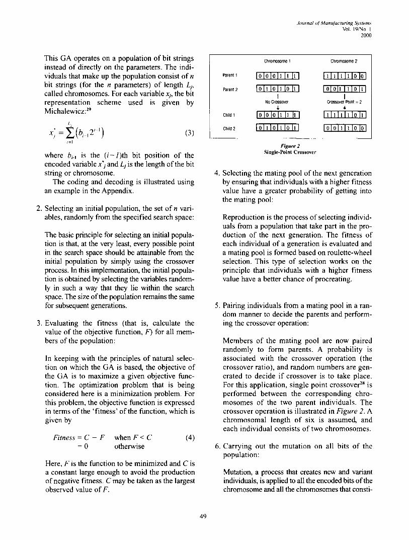
This GA operates on a population of bit strings instead of directly on the parameters. The individuals that make up the population consist of n bit strings (for the n parameters) of length Lj, called chromosomes. For each variable x~, the bit representation scheme used is given by Michalewicz: 29

x,:~.,(b,_,2 i-' ) (3) i=1

where bi_~ is the ( i -1) th bit position of the encoded variable x'~ and Lj is the length of the bit string or chromosome.

The coding and decoding is illustrated using an example in the Appendix.

2. Selecting an initial population, the set of n variables, randomly from the specified search space:

The basic principle for selecting an initial population is that, at the very least, every possible point in the search space should be attainable from the initial population by simply using the crossover process. In this implementation, the initial population is obtained by selecting the variables randomly in such a way that they lie within the search space. The size of the population remains the same for subsequent generations.

3. Evaluating the fitness (that is, calculate the value of the objective function, F) for all members of the population:

In keeping with the principles of natural selection on which the GA is based, the objective of the GA is to maximize a given objective function. The optimization problem that is being considered here is a minimization problem. For this problem, the objective function is expressed in terms of the 'fitness' of the function, which is given by

F i t n e s s = C - F w h e n F < C (4) = 0 otherwise

Here, F is the function to be minimized and C is a constant large enough to avoid the production of negative fitness. C may be taken as the largest observed value of F.

Chromosome 1 Chromosome 2

Parent1 10101011 I1 Ill I l l l l l l l l o l o l

Parent 2 I0111011 I0 I l l IoloIz I = l o l l I I I

No Crossover Crossover Point = 2

c,,,~1 Io lo lo l l I1 I l l I11111111o111

c,,,~2 I o l l l o I l l o l l l I010111110 Iol

Figure 2 Single-Point Crossover

. Selecting the mating pool of the next generation by ensuring that individuals with a higher fitness value have a greater probability of getting into the mating pool:

Reproduction is the process of selecting individuals from a population that take part in the production of the next generation. The fitness of each individual of a generation is evaluated and a mating pool is formed based on roulette-wheel selection. This type of selection works on the principle that individuals with a higher fitness value have a better chance of procreating.

.

.

Pairing individuals from a mating pool in a random manner to decide the parents and perform- ing the crossover operation:

Members of the mating pool are now paired randomly to form parents. A probability is associated with the crossover operation (the crossover ratio), and random numbers are generated to decide if crossover is to take place. For this application, single point crossover 2s is performed between the corresponding chromosomes of the two parent individuals. The crossover operation is illustrated in Figure 2. A chromosomal length of six is assumed, and each individual consists of two chromosomes.

Carrying out the mutation on all bits of the population:

Mutation, a process that creates new and variant individuals, is applied to all the encoded bits of the chromosome and all the chromosomes that consti-

49

Journal of Manufacturing Systems Vol. 19/No. 1 2000

?iiiiiiiiiiiiSi ...... Cylindricit tolerance

Figure 3 Definition of Cylindricity Toleranceover

tute the individual. The bit is flipped only if a random number generated is less than a specific value (called the mutation rate).

7. Decoding and evaluating the fitness of the individuals in the new population generated after the crossover and mutation operations.

Steps 4-7 are repeated iteratively until the optimal solution is obtained or a termination con- dition is satisfied.

3.1 C o n s t r a i n t H a n d l i n g The parameters that are involved in the problem

have specified maximum and minimum bounds. These constraints have to be met at all stages in the GA implementation. While generating the initial population, the variables are selected from the constrained search space so as to satisfy the constraints. However, as a result of crossover or mutation, individuals may be produced that violate the constraints. This problem is handled by following the 'death penalty' approach in which these individuals are rejected and a fresh individual is generated in its place. 27

3.2 Termination Criteria To terminate the algorithm at the right time, there

is a need for a criterion that attempts to check whether the algorithm has converged at the end of each generation. To check for convergence of the fitness value, the following conditions are checked at the end of each generation (after the initial five generations):

MFi > MFi.5 (5)

(MFi" MFi.5) / MFi < e (6)

where MF; = maximum fitness value of the ith generation and e = a small percent of the maximum fitness at the ith generation (MF~" (0.0001/100)).

If these conditions are satisfied at any stage of the GA, the algorithm is stopped, and it is concluded that the function has attained its minimal value and further iterations will not result in any significant improvement in the solution. If even after the 50th generation convergence is not observed, the algorithm is forced to stop so that it can compete, with respect to computational time, with other methods that solve the same problem.

4. Minimum Zone Tolerance Formulation

The ANSI ~ standards require the establishment of an ideal feature (corresponding to the form feature being evaluated) that completely encloses all the data points. The minimum zone method aims at minimizing the maximum deviation of the feature from the ideal feature estimated. The application of this technique to the case of cylindricity tolerance is described first and in greater detail as this problem is difficult in its deterministic form, and the power of the genetic algorithm is best illustrated in this case. The circularity and flatness problems are then solved. Finally, the straightness problem is described and thus a robust optimization procedure is described that can be applied to all form tolerance evaluation problems.

4.1 Cylindricity In the case of cylindricity, a pair of coaxial cylin-

ders has to be determined that completely enclose the data sets and have a minimal radial separation. This radial separation is the final cylindricity tolerance (Figure 3). The axis needs to be established in order to determine the coaxial cylinders. The minimum zone formulation is given by the following:

F = min [max ( d i ) - min (di)] (7) for i = I to number of points (n)

where co / s o~ J k d = cos~ cosy (8)

x - a y - b .

where d is the normal (radial) distance of any point in the data set from the axis, a, 13, and y are the direction angles of the axis, (a, b, 0) are the coordinates of a point in the X-Y plane through which the axis passes, and i, j, k are the unit vectors in thc X, Y, and Z directions.

The limits on the direction angles are as follows:

aa < ai <- b, (9)

50

.hmrnal o[ Manufacturing Systems Vol. 19/No. l

2000

Z

_ _ .

Juadrant III / /.//// J~X /"/

• Cylinder axis

.IiY ! ~ Quadrant I

Quadrant IV

Figure 4 Maximum Possible Search Space for a and b

a~ < 13,. < b~ (10)

Further,

cosZcxi + cosZ13; + cosZ~h = 1 (11)

There are four variables that need to be varied in their respective bounds to arrive at the minimal value for the function F. Reasonable bounds for the variables a and b need to be selected. These bounds should be large enough so that there is no possibili- ty that the actual optimal variables lie outside this bound, but also of a reasonable size so that the algorithm is computationally efficient. A search space is defined that is formed by all the acceptable values of the four parameters involved. The GA implemented ensures that the search space is never violated and the solution is always valid.

Each of the four variables is encoded. The individual in this case consists of four chromosomes, each representing a variable. Each individual is a prospective solution to the problem. Many such randomly generated individuals constitute the initial population. The GA is then put to work and attempts to arrive at the optimal value of these four variables, which minimizes the objective function specified. The fitness function is defined as follows:

Fitness = C - F when F < C (12) -- 0 otherwise

The constant C has to be evaluated for each data set. In this implementation, the GA is first run with the fitness value the same as the function F. The largest observed value of F (after a fixed number of generations) is extracted and assigned to C. Then the GA is run for the correct fitness function (which is C - F).

e,}

12~ 10. 8, 6 4~ 21 0 .

2.5 2 25 . "2

1 . 5 - . .. 1 . 5

1 1 ~ 0.5 0.5 Alpha

F/gure 5 Search Space for ct and 13 to Determine Cylindricity Tolerance

The selection of the variable bounds is better understood using the following illustration:

For the data sets used, the bounds for the four variables are specified as follows:

45 ° < a < 135 °

45 ° < 13 < 135 °

- 0 . 5 < a < 1.5

- 1 . 0 < b < 1.0 (13)

The range of a and 13 is chosen such that the expres- sion relating the direction cosines is not violated. The radian magnitude of the angles is used in the algorithm. The range of a and b is chosen in the following manner: all the data points are projected in the X - Y

plane, and this plane is divided into four quadrants with the mean (O) of the projected data set as the origin. The points in each quadrant that is farthest from O are determined and their distance from O noted. Each of these points is joined in order, and a quadrilateral is formed with these points as the vertices. This quadrilateral is the largest possible search space for a and b. To improve the efficiency of the search, a smaller rec- tangular region is chosen within this quadrilateral. This is done by considering the maximum (sin,,) and minimum lengths (s=l,) of the quadrilateral. A rectan- gle with its center as O is drawn with sides s=,~ and Smi,, and this is the new modified search space for a and b. This is illustrated in Figure 4. The search space for a and 13 for the mean values of a and b for a sample data set are shown in Figure 5.

51

.lournal of Manufacturing Sy.s'tems Vol. 19/No. 1 2000

Table 1 Comparison of Results for Cylindricity

Data Set Size of Least-Squares Voronoi All , thin Number Data Set Method Method Mlflhod

1 10 0.65508 0.2011 2 15 2.10783 2.0000

3 20 1.20353 1.1498

4 25 2.16843 1.8801

5 [Ref. 14] 64 0.06935 0.028813 [14] 0.027351

Circularity tolerance /

Figure 6 Definition of Circularity Tolerance

At the end of each generation in the algorithm, the fitness of the individuals is evaluated and the best individuals are identified. Each individual is a prospective solution to the minimization problem. This iterative process of producing new generations is halted when the termination criteria are satisfied. The best individual (a set of four variables) produced by the process is the solution to the problem.

The GA was run for five sample data sets, and the results are tabulated in Table 1. It can be seen that the results obtained from GA are much more accurate than the least squares and the Voronoi method, ~4 and it works for any data set, unlike the Voronoi diagram method.

4.2 Circularity A pair of concentric circles, having minimal radi-

al separation and enclosing all the points in the data set, is established to evaluate the circularity tolerance. The definition of circularity tolerance is illustrated in Figure 6. The final tolerance value is given by the radial difference. Mathematically, a circle can be represented as follows:

r : ~ f ( x - a ) 2 + ( y - b ) 2 (14)

where (a, b) are the coordinates o f the center of the

( / Figure 7

Maximum Possible Search Space for a and b

"-~.

\ \ j j - - ' ~

b -5 -5 a

Figure 8 ,Search Space for a and b to Determine Circularity Tolerance

circle, and r is the radius of the circle. The minimum zone formulation for this case is

given by the following:

F = min [max (ri) - min (r)] for i = 1 to number of points (n)

subject to

(15)

- h < ai < h (16)

- h < bi < h (17)

The value h is computed as follows: the mean center for the data set is computed and the distance of the farthest point (r,,,,) and the nearest point from the center (r,.~.) are noted. Then

h = 2(rm.x - r,,i,) (18)

and the search space for a is a square of side h with the mean center (C,.) at the center of the square. This search space is shown in Figure 7. The variables a and b are encoded to produce two chromosomes which together constitute an individual. Figure 8

52

Journal of Manufacturing Systerns Vol. 19/No. I

200t)

Table 2 Comparison of Results for Circularity

Minimum Maximum Voronoi (~mJl@. Data Set Size of Least-Squares Circumscribing Inscribing Diagram Number Data Set Method Method Method Method

I. [Ret: 12] 8 2.3719 2.6095 2.3505 2.2432 [ 12] ~ III I J ~1

2. I 0 0.2299 0.2691 0.2385 0.2288 0,,;~11~

3. 12 0.1576 0.1689 0.1454 0.1449 0 . 1 4 ~ l u i i

4. 15 1.7262 1.6530 1.6618 1.5694 1.5705

5. 20 1.7449 1.7382 1.7287 1.6711 1.6715

shows the search space for a and b that the GA cov- ers. The fitness function is o f the following form:

Fitness -- C - F (19)

where C is a constant. Five sets o f data with varying number of sampled

points were taken up for simulation, and the results o f the runs are presented in Table 2. It can be seen that the results are better than the least-squares, MCC, and M|C methods and are comparable to the Voronoi diagram method.

4 . 3 F l a t n e s s

For flatness tolerance, a pair of planes that enclose all the data points needs to be established (Figure 9).

An additional constraint is that the distance between these planes should be the minimum possible (the flatness tolerance value). The equation of a plane in para- metric form can be represented as follows:

p = xcosa +ycos13 + zcos~ (20)

where p is the perpendicular distance o f the plane from the origin and ec 13, and ~/ are the direction angles of the plane.

Figure 9 Definition of Flatness Tolerance

The minimum zone equation for this case is given by the following:

F = min [max (pl) - m i n (Pi)] for i = 1 to number of points (n)

subject to

(21)

45 ° < eti < 135 °

45 ° < 13i< 135 °

cos2cti + cosZ13i + cos2~/i = l (22)

The variables et and 13 are encoded to produce two chromosomes which together make up an individual, and the search zone for these variables is shown in Figure 10. The fitness function that is minimized by the GA is o f the form

Fitness = C - F (23)

where C is a constant. The first four data sets provided in Traband et al. 6

were used to compare the results of GAs with those

3.5

3. 2.5

i

c

1.5

1. 0.5

0 2.5

1 5" ' 1 . 5 1 " 1

Beta 0.5 "0,5 Alpha

2.5

Figure i0 Search Space to Evaluate Flatness Tolerance

53


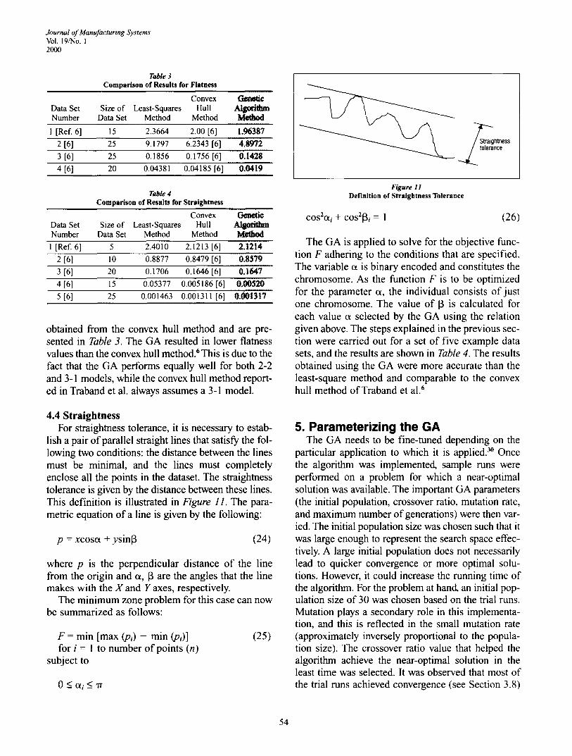
Table 3 Comparison of Results for Flatness

Convex Cnm~ic Data Set Size of Least-Squares Hull A l ~ l t l m Number Data Set Method Method Mclhod

1 [Ref. 6] 15 2.3664 2.00 [6] 1.96387

2 [6] 25 9.1797 6.2343 [6] 4.8972 3 [6] 25 0.1856 0.1756 [6] 0.1428 4 [6] 20 0.04381 0.04185 [6] 0.0419

Table 4 Comparison of Results for Straightness

Convex C~netic Data Set Size of Least-Squares Hull Number Data Set M e t h o d M e t h o d Melhod 1 [Ref. 6] 5 2.4010 2.1213 [6] 2.1214

2 [6] 10 0.8877 0.8479 [6] 0.8579 3 [6] 20 0.1706 0.1646 [6] 0.1647 4 [6] 15 0.05377 0.005186 [6] 0.00520 5 [6] 25 0.001463 0.001311 [6] 0.001317

obtained from the convex hull method and are presented in Table 3. The GA resulted in lower flatness values than the convex hull method. 6 This is due to the fact that the GA performs equally well for both 2-2 and 3-1 models, while the convex hull method reported in Traband et al. always assumes a 3-1 model.

4.4 Straightness For straightness tolerance, it is necessary to estab-

lish a pair o f parallel straight lines that satisfy the following two conditions: the distance between the lines must be minimal, and the lines must completely enclose all the points in the dataset. The straightness tolerance is given by the distance between these lines. This definition is illustrated in Figure 11. The para- metric equation of a line is given by the following:

p = xcosc~ + ysin13 (24)

where p is the perpendicular distance o f the line from the origin and a , 13 are the angles that the line makes with the X and Y axes, respectively.

The min imum zone problem for this case can now be summarized as follows:

F = min [max (p,) - min (p,)] for i = 1 to number o f points (n)

subject to

(25)

0 < or,. _< -rr

Figure I 1 Definition of Straightness Tolerance

cos2a; + cos~13i = I (26)

The GA is applied to solve for the objective function F adhering to the conditions that are specified. The variable a is binary encoded and constitutes the chromosome. As the function F is to be optimized for the parameter c~, the individual consists o f just one chromosome. The value of 13 is calculated for each value a selected by the GA using the relation given above. The steps explained in the previous section were carried out for a set of five example data sets, and the results are shown in Table 4. The results obtained using the GA were more accurate than the least-square method and comparable to the convex hull method ofTraband et al. 6

5. Parameterizing the GA The GA needs to be fine-tuned depending on the

particular application to which it is applied. ~ Once the algorithm was implemented, sample runs were performed on a problem for which a near-optimal solution was available. The important GA parameters (the initial population, crossover ratio, mutation ratc, and maximum number of generations) were then varied. The initial population size was chosen such that it was large enough to represent the search space effec- tively. A large initial population does not necessarily lead to quicker convergence or more optimal solutions. However, it could increase the running time of the algorithm. For the problem at hand, an initial population size of 30 was chosen based on the trial runs. Mutation plays a secondary role in this implementation, and this is reflected in the small mutation rate (approximately inversely proportional to the population size). The crossover ratio value that helped the algorithm achieve the near-optimal solution in the least time was selected. It was observed that most of the trial runs achieved convergence (see Section 3.8)

54

Journal of Manufacturing Systems Vol. 19/No. I

2000

well before the 50th generation was produced. Hence, the maximum number of generations the algorithm is allowed to generate was fixed at 50. In all the examples that have been run, the same values of the parameters have been used, as follows:

Initial Population Size = 30 Crossover Ratio = 0.6 Mutation Rate = 0.033 Maximum Number of Generations = 50

6. Discussion of Results A genetic algorithm was implemented to tackle the

nonlinear optimization problem that arises in the evaluation of form tolerances. The four primary form tolerances, namely straightness, flatness, circularity, and cylindricity, were considered in this implementation. All the GA algorithms were implemented on a SUN Spare 5 Workstation using MATLAB 5.0. The results obtained for each of these cases are compared with those obtained from the existing methods.

The convex hull method is the most accurate method currently to evaluate straightness. 6 A set of five examples was taken from Traband et al. 6, and the GA was applied to solve for the straightness values. It can be seen that the results obtained using the GA are comparable to those obtained by the convex hull method.

The flatness values obtained by this method are better than both the convex hull and the least- squares methods. This is because the planes that are determined are not chosen in a deterministic manner from a predefined set (as in the case of the 3-1 model of the convex hull method) but are chosen from a much larger set of possible plane configura- tions. This ensures that 3-1, 1-3, and 2-2 models are taken into consideration for the evaluation.

In the case of circularity, the GA results are comparable to those obtained by the Voronoi diagram method and are better than the least-squares method, minimum circumscribing circle method, and the maximum inscribed circle method.

The power of this GA implementation can be fully visualized in the case of cylindricity. At the present time, there are no deterministic methods available to completely solve the cylindricity problem. In the GA method, the data points need not be collected at sections perpendicular to the Z axis; the effect of the errors involved in the data collection

Table 5 Sample of CPU Times on a SUN Spare Station

Tolerance Ct~ The, Data Set Type of Size of Value ~¢. Number Form Data Set Obtained ( ~

Tolerance by GA Spat, e 5)

1. [From Table 1] Cylindricity l0 0.2011 2.646 2. [Table 1] Cylindricity 15 2.0000 3,969 3. [Table 2] Circularity 8 2.2422 1.871 4. [Table 2] Circularity 10 0.2307 2,339 5. [Table 3] Flatness 15 1.96387 3,$58 6. [Table 3] Flatness 25 4.8972 5.93 7. [Table 4] Straightness 10 0.8579 1.378 8. [ Table 4] Straightness 20 0.1647 2,756

process does not affect the tolerance value at all. The data points can be collected from anywhere on the surface of the cylinder. An axis is fitted to the given data points, and the orientation and position values of the axis that give the minimum tolerance value are determined. This method was also tested on the data set given in Roy and Xu, 14 and it can be seen that the results obtained by this method are better than those of the Voronoi diagram method.

Table 5 lists the CPU time that the genetic algorithm takes to arrive at the tolerance value for the various form tolerances. The CPU time for two data sets for each form tolerance type is reported. This illustrates, as expected, that the time taken for the GA to arrive at a solution increases as the size of the data set increases.

7. Conclusions The GA used here does not need any significant

preprocessing for calculating the tolerances. It is a very robust method and can be applied successfully to all form tolerances, from the complex cases of evaluating cylindricity and flatness to the relatively simple problem of straightness evaluation. This method is fast and accurate in spite of it being an iterative method. The results presented in this paper illustrate the poten- cy of this particular approach to the problem of form tolerance evaluation. The method provides very accurate results, and it truly optimizes any objective function without getting stuck at the local optima. This method can be made as fast as possible by reducing the search space. This involves providing reasonable constraints for the variables involved in the search. The GA approach is also not affected by the size of the data sets.

55


Acknowledgments The research reported in this paper has been par-

tially supported by the National Science Foundation under grant no. DMI 9523120.

References I. American National Standards Institute, "Dimensioning and Tolerancing,

ANSI Y14.5M-1994" (New York: American Society of Mechanical Engineers, 1994).

2. ISO/DIS 1101, Technical Drawing, Tolerances of Form and Position (lnt'l Organization for Standardization, 1972).

3. T.S.R. Murthy and S.Z. Abdin, "Minimum Zone Evaluation of Surfaces,"Int '1 Journal of Machine Tool Design Research (v20, 1980). pp 123- 136.

4. M.S. Shunmugam, "Comparison of Linear and Normal Deviations of Forms of Engineering,"Precision Engg. (v9, n2, 1987), pp96-102.

5. K. Lai and J. Wang, "A Computational Geometry Approach to Geometric Tolerancing,"Tmns. of 16th North American MJg. Research Omf (1988), pp376-379.

6. Mark Traband et al., "Evaluation of Straightness and Flamess Tolerances Using the Minimum Zone,"Mfg. Review (v2, n3, 1989), pp 189-195.

7. Hossein H. Charagi et al., "Straightness and Flatness Tolerance Evaluation: An Optimization Approach"Precision Engg. (vlS, nl, 1996), pp30-37.

8. S.T. Huang et al., "A New Minimum Zone Method for Evaluating Flatness Errors,"Precision Engg (v15, hi, 1993), pp25-32.

9. T. Kanada and S. Suzuki, "Evaluation of Minimum Zone Flatness by Means of Nonlinear Optimization Techniques and Its Verification"Precision Engg. (v15, nl, 1993), pp93-99. 10. R.C. Melville, "An Implementation Study of Two Algorithms for the Minimum Spanning Circle Problem,'in Computational Geometr3; G.T. Toussaint, ed. (Elsevier Science Publishers, 1985), pp267-285. 11. H. Chang and T.W. Lin, "Evaluation of Circularity Tolerance Using Monte Carlo Simulation for Coordinate Measuring Machines,"lnt 7Journal o/ Production Research (v31, 1992), pp2079-2086. 12. U. Roy and X. Zhang, "Establishment of a Pair of Concentric Circles with Minimum Radial Separation for Assessing Roundness Error,"Computer AidedDesign (v24. 1992), ppl61-168. 13. U. Roy and X. Zhang, "Development and Application of Voronoi Diagrams in the Assessment of Roundness Error in an Industrial Environment,"Computers in lndus'trial Engg. (v26, nl, 1992), ppl 1-26. 14. U. Roy and Y. Xu, "Form and Orientation Tolerance Analysis for Cylindrical Surfaces in Computer-Aided Inspection,"Computers in Ind~s't- O' (v26, 1995), ppl27-134. 15. Jiing-Yih Lai and Ing-Hong Chen, "Minimum Zone Evaluation of Circles and Cylinders,"lnt '1 Journal of Machine Tools Design and Research (v36, n4, 1996), pp435-451. 16. T.S.R. Murthy, "A Comparison of Different Algorithms for Cylindricity Evaluation,"lnt '1 Journal t f Machine Tools Design Research (v22, n4, 1982), pp283-292. 17. Makoto Fukuda and Akira Shimokohbe, "Algorithms for Form Error Evaluation - Methods of the Minimum Zone and the Least Squares,"Pn~c. of Int'l Symp. on Metrology for Quality Control in Production (Tokyo, 1984)o pp 197-202. 18. D.G. Chetwynd, "'Application of Linear Programming to Engineering Metrology,"P~r~c. of the Institution of Mechanical Engineers (v 199, 1985), pp93- 100. i 9. Yu Wang, "Minimum Zone Evaluation of Form Tolerances"Mfg. Review (v5, n3, 1992), pp213-220. 20. Kirsten Carr and Placid Ferriera, "Verification of Form Tolerances, Part I: Basic Issues, Flatness and Slraightness,"Prccision Engg. (v17, n2, 1995), ppl31-143. 21. Kirsten Carr and Placid Ferriera, "Verification of Form Tolerances, Part II: Cylindricity and Straightness of a Median LineSPrecision Engg. (v17, n2, 1995), pp144-158. 22. A. Grauel, "optimization with Evolutionary Algorithms:'Proc. of 3rd

lnt'l Conf. on Computer Integrated Mlg. (v3. 1995), pp71-80. 23. W. Wienhoh, "A Refined Genetic Algorithm for Parameter Optimization Problems,"Proc. of 5th lnt'l Conf. on Genetic Algorithms (1993), pp589-596. 24. S. Kwong, A.C. Ng, and K.E Man, "'Improving Local Search in Genetic Algorithms for Numerical Global Optimization Using Modified GRll)-Point Search Technique,"5th Int'l (7ont~ on Genetic Algorithms in Engineering Systems: Innovations and Applications (1995). 25. M. Srinivas and LM. Patnaik, "Genetic Algorithms. A Survey."lEEE Trans. on Computerg (June 1994), pp 17-26. 26. J. Lee and G.E. Johnson, "Optimal Tolerance Allocation Using Genetic Algorithm and Monte Carlo Simulation,"Computer Aided Design (~25. n9. Sept. 1993), ppr01-611. 27. Z. Michalewicz, l). Dasgupta, R.G. Le Richc, and M. Schocnaucr. "l.;volutionary Algorithms for Constrained Engineering Problems,"Computers in Indtt*trial Engg. (v30, n4, 1996), pp851-870. 28. DE. Goldbcrg, Genetic Algorithms m Search. Optimization and Machine Learning (Addison-Wesley, 1989). 29. Z. Michalewicz, Genetic Algorithms - Data Structures - Evolutionary Programmmg (Springer-Verlag, 1994). 30. I.. Davis, Hand&ink ~/ Genetic Algorithms (Van Nostrand Reinhold, 1991 ).

Appendix Illustration of Genetic Coding and Decoding

Assume that the length of the chromosome defined to specify a particular parameter is 10. Consider the variable a (an angle in radians). For this example, let the range in which this variable lies be 0.7854 and 2.3562. For the production of the initial population, many different values of a are chosen such that they lie in the constrained range, l fa value of 1.232 is chosen, then it is converted to a chromosome for the application of the GA as under:

1.232 * 2 ~l°m [from Section 3.1, Eq. (3)]

1.232 * 512 = 631 (scaled variable)

Binary (631) • 10001110111

In a similar fashion, all the other variables that constitute an individual are coded and used to produce the initial population. These variables need to be converted into their decimal representation to evaluate the fitness of the function. Consider the variable a after one generation has been generated using the GA. Let the chromosome that represents a be:

1000000010

Converting the chromosome to base 10 (decimal) representation yields:

514

56

Journal o/'Manufacturing Systems Vol. 19/No. I 2000

Multiplying this by (2.3562 - 0.7854) / (2 ~° - 1) [from Section 3.1, Eq. (5)]:

514 * 0.0015355 = 0.78925

The actual value of the variable is:

0.7538 + 0.78925 = 1.54305

The other chromosomes are similarly decoded and fed into the objective function. Decoding is performed only for objective function evaluation. For the purpose of application of the genetic algorithm and transfer of information between generations, the variables are always kept in their binary format.

Authors' Biographies Rohit Sharma is currently working for an information technology consult-

ing firm in Cincinnati, OH. He obtained his master's degree in mechanical engineering from the University of Cincinnati in 1997 and has a bachelor's degree from the Indian Institute of Technology (Madras, India). His research interests include computer-aided design and manufactunng, manufacturing systems, machine vision systems, and optimization techniques.

Karthik Rajagopal received his master's degree in industrial engineering from the University of Cincinnati. He had received his bachelor of technology degree in mechanical engineering from the Indian Institute of Technology (Madras, India). Hc is currently working as a software con- sultant with i2 Technologies (Irving, TX). His research interests include metrology, tolerancing, machine vision, and optimization methods.

Sam Anand received his BE (Honors) degree in mechanical engineering from the University of Madras, India, an ME (Distinction) in mechanical engineering from the Indian Institute of Science, and an MS and PhD in industrial engineering from the Pennsylvania State University. Dr. Anand is currently an associate professor and director of the Computer-Aided Manufacturing Laboratory in the industrial engineering program at the University of Cincinnati. His research interests are in the areas of feature-based design and manufacturing, process planning and costing, tolerancing and computational metrology, optimization in manufactunng, and machine vision inspection. Dr. Anand has published several archival papers in these research areas, and he is a member of SME. liE, and Tau Beta Pi.

57

A genetic algorithm based approach for robust evaluation of form tolerances

Documents

Transcript of A genetic algorithm based approach for robust evaluation of form tolerances