A robust algorithm for DTM generation from Aerial Laser ...

ent 108 (2007) 9–23www.elsevier.com/locate/rse

Remote Sensing of Environm

Repetitive interpolation: A robust algorithm for DTM generation from AerialLaser Scanner Data in forested terrain☆

Andrej Kobler a,⁎, Norbert Pfeifer b, Peter Ogrinc a, Ljupčo Todorovski c,Krištof Oštir d, Sašo Džeroski c

a Slovenian Forestry Institute, Vecna pot 2, 1000 Ljubljana, Sloveniab Vienna University of Technology, Austriac Jozef Stefan Institute Ljubljana, Slovenia

d Scientific Research Centre of the Slovenian Academy of Sciences and Arts, Slovenia

Received 10 October 2005; received in revised form 24 October 2006; accepted 27 October 2006

Abstract

We present a new algorithm for digital terrain model (DTM) generation from an airborne laser scanning point cloud, called repetitiveinterpolation (REIN). It is especially applicable in steep, forested areas where other filtering algorithms typically have problemsdistinguishing between ground returns and off-ground points reflected in the vegetation. REIN can produce a DTM either in a vector grid orin a TIN data structure. REIN is applied after an initial filtering, which involves removal of all negative outliers and removal of many, but notnecessarily all, off-ground points by some existing filtering algorithm. REIN makes use of the redundancy in the initially filtered point cloud(FPC) in order to mitigate the effect of the residual off-ground points. Multiple independent random samples are taken from the initial FPC.From each sample, ground elevation estimates are interpolated at individual DTM locations. Because the lower bounds of the distributions ofthe elevation estimates at each DTM location are almost insensitive to positive outliers, the true ground elevations can be approximated byadding the global mean offset to the lower bounds, which is estimated from the data. The random sampling makes REIN unique among themethods of filtering airborne laser data. While other filters behave deterministically, always generating a filter error in special situations, inREIN, because of its random aspects, these errors do not occur in each sample, and typically cancel out in the final computation of DTMelevations. Reduction of processing time by parallelization of REIN is possible. REIN was tested in a test area of 2 hectares, encompassingsteep relief covered by mixed forest. An Optech ALTM 1020 lidar was used, with a flying height of 260–300 m above the ground, the beamdivergence was 0.3 mrad, and the obtained point cloud density for the last returns was 8.5 m−2. A DTM grid was generated with 1 mhorizontal resolution. The root mean square elevation error of the DTM ranged between ±0.16 m and ±0.37 m, depending on REIN samplingrate and number of samples taken, the lowest value achieved with 4 samples and using a 23% sampling rate. The paper also gives a shortoverview on existing filtering algorithms.© 2006 Elsevier Inc. All rights reserved.

Keywords: Lidar; Airborne laser scanning; Digital terrain modeling; Forest

1. Introduction

Airborne laser scanning (ALS), also termed airborne lidar(Light Detection And Ranging), is one of many laser remote

☆ The work on this paper was partly performed at alp-S, Centre for NaturalHazard Management, Innsbruck, Austria.⁎ Corresponding author. Tel.: +386 1 2007835.E-mail address: [email protected] (A. Kobler).

0034-4257/$ - see front matter © 2006 Elsevier Inc. All rights reserved.doi:10.1016/j.rse.2006.10.013

sensing techniques (Measures, 1992). By measuring the roundtrip time Δt of an emitted laser pulse from the sensor to areflecting surface and back again, the distance from the sensorto the surface d is determined using the known speed of light cin air: d=c Δt / 2. For measuring the topography of the Earthsurface from an aircraft, typically an airplane, the position andattitude of the platform have to be known. These parameters aredetermined with GPS and IMU, Ip et al. (2004). Throughperiodical deflection of the emitting direction across the flight

mailto:[email protected]

http://dx.doi.org/10.1016/j.rse.2006.10.013

Fig. 1. Filtering of ALS data for ground detection. In (a) the structure element shows the admissible height differences based on distance (units are meters). In(b) a point cloud is shown in a profile with ground, a roof and vegetation points, where at two specific points (black dots) windows are centered. In the rightcase two points (bold circles) are identified as not-ground points. In (c) a triangle of previously identified ground points (B1, B2, B3) is shown and measures(α1, α2, α3) to determine, if the investigated point (P) shall be classified as ground point. In (d) a first, rough surface model is shown as the upper linecomputed from the entire point set (profile view) and the lower line shows the DTM in the next iteration. In (e) a weight function is plotted which takes asinput the residuals, i.e., the signed distance of the points to the surface. In (f ) the segmentation of an ALS pointset is shown in a 3D view with different greytones for different segments.

10 A. Kobler et al. / Remote Sensing of Environment 108 (2007) 9–23

path by an oscillating or rotating mirror and by the forwardmotion of the aircraft, a dense cloud of points is sampled on theEarth’s surface in the form of a swath. Multiple flight lines arenecessary to cover a large area. Commercial airborne laserscanners can operate from heights up to 5000 m, reach ameasurement frequency of 100,000 points per second andhigher, and a height accuracy of a few cm. This leads to a typicalpoint density of one point per m2, but often a higher density isachieved. Lower densities are not untypical either, resultingfrom large flying heights, from fast fixed wing aircraft operationand low pulse repetition rates.

Airborne laser scanning is different to radar because thefootprint of the emitted signal is much smaller, Bufton (1989).Radar measurement therefore cannot provide such a highspatial resolution as laser measurements. With SAR (syntheticaperture radar), and especially InSAR (interferometric SAR)resolution can be increased, but the accuracy of lasermeasurements is not reached (Andersen et al., 2004). Alaser shot can penetrate the tree crowns, i.e., look throughsmall gaps in the foliage, and reach the ground. Therefore, thedistance to the ground below trees can be measured. Passiveoptical remote sensing techniques for inferring terrain ele-

vation, i.e., photogrammetry, require that (1) enough sun lightis scattered back from one ground position onto (2) twoimages, which makes the measurement of ground belowcanopy elevation from imagery almost impossible (Kraus &Pfeifer, 1998).

Because of its immediate generation of 3D data, high spatialresolution and accuracy, ALS data is becoming popular for thereconstruction of digital terrain models (DTM; Sithole &Vosselman, 2004) and virtual city models (Kaartinen et al.,2005). Since the lidar signal has the ability to pass through gapsin foliage and reflect from different parts of trees it is also usedfor measuring tree height and estimating other forest standparameters (Hyyppä et al., 2004).

The backscattering mechanism utilized in airborne laserscanning is diffuse reflection. The (laser) light coming from onedirection (i.e., from the sensor) is scattered at the reflecting surfaceinto all directions. A small portion of the emitted energy thereforetravels back to the sensor where the runtime is measured. As thediameter of the laser pulse is not infinitely small but has a certainfootprint, typically in the range of 50 cm to 1 m, several objectscan be the source of the backscattered signal. Modern receiverscan record multiple echoes, e.g., the first, second, third, and last

11A. Kobler et al. / Remote Sensing of Environment 108 (2007) 9–23

echo. These discrete return small footprint systems have to bedistinguished from the systems recording the entire backscatteredwaveform (Wagner et al., 2006), and large footprint systems as,e.g., NASA's Vegetation Canopy Lidar (VCL; Blair et al., 1999),and GLAS (Zwally et al., 2002), instruments. Therefore, ALSprovides points measured on objects between the sensor and theground surface, depending on where the laser beam is reflected.As it can be reflected by power lines, vegetation leaves, houseroofs, etc., many points do not lie on the ground surface.Classification of these points into ground and object (off-terrain)points is called filtering. This is an essential step necessary fordigital terrain model (DTM) generation, but also for furtherreconstruction of topographic features (houses, power-lines, etc.)that is often performed relative to the DTM, using a normalizedsurface model.

Due to multi-path reflection, points which apparently liebelow the Earth's surface, can also be obtained. If a portion ofthe emitted energy travels from the sensor to the ground surfaceand not immediately back to the receiver but bounces to anothersurface before, the runtime measured corresponds to a distancewhich is longer than the platform ground distance and the pointposition will be computed below the ground.

As the filtering methods operate purely in an automatedmode, i.e., with one set of parameters for large areas (typicallyseveral km2 to several hundreds of km2) the resulting DTMsare not optimal in all areas, requiring interactive fashions ofparameter testing and manual correction of the results. Steepwooded terrain is especially considered as a problem infiltering. Therefore, there is a tangible need for precise ter-rain information in difficult relief. Within this paper we pre-sent a new filtering algorithm for steep relief under denseforest cover, where other filtering algorithms typically haveproblems distinguishing between ground returns and pointsreflected in the vegetation. The algorithm is also new in thesense that it cannot be put into any one of the four maincategories specified in Section 2. On one hand it is able to dealwith sparse ground returns under dense forest canopy, but onthe other hand also with highly redundant ground returns inforest openings. The problem of negative outliers, originatingfrom multi path reflections, is also addressed by this newalgorithm.

The motivation for our work was to get high quality terrainelevations as basis for further forestry related analysis of lidardata. The specific contribution of this work is a method whichprovides a precise and reliable DTM even if the laser scannerground hits are sparse and very irregularly distributed.Variation in the number of ground hits may vary on all scalesas it is affected by vegetation type, terrain characteristics, andscanner characteristics. The portion of points on the grounds isaffected by the vegetation, where different tree species lead todifferent penetration rates, and by the sampling pattern of thelaser sensor, which does not necessarily lead to equal pointpostings on the ground. This results in higher and lower pointdensities, respectively, within one swath. Depending on theairborne laser scanner in use, the point density becomes higher(oscillating mirror) or lower (rotating mirror) at the sides of theswath.

Section 2 of this paper summarizes the existing methods offiltering, Section 3 illustrates and explains in detail the newfiltering algorithm, in Section 4 the test area and the input dataare described, Section 5 lists and discusses the algorithmresults for the test area, and finally, Section 6 draws theconclusions.

2. The state of the art in lidar filtering

Different concepts for filtering have been proposed so far.The first group of filters got its name from mathematicalmorphology (Haralick & Shapiro, 1992) and is used inmorphological filtering (Vosselman, 2000). A structure element,describing admissible height differences depending on hori-zontal distance is used (Fig. 1a). The smaller the distancebetween a ground point and its neighboring points, the lessheight difference is accepted between them. This structureelement is placed at each point so off-terrain points areidentified as those above the admissible height difference.The structure element itself could be determined from terraintraining data resulting in an optimal structure element tominimize type I and type II errors, or it could be obtained frommaximum terrain slope assumptions. Variants of the morpho-logical filtering are described by Sithole (2001), where thestructure element depends on terrain shape. For steeper areashigher admissible height differences are allowed. The steepnessitself is determined in an averaging procedure over large areas.A similar idea is presented by Zakšek and Pfeifer (2006) wherethe structure element is inclined as a whole in order to follow theterrain, i.e., the rotational symmetry around the z-axis is lost.The reason is that height differences downwards have differentcharacteristics compared to the upwards height differences,which is not considered in the other morphological filters.Kilian et al. (1996) use multiple structure elements of differentsize in the morphological operation Opening. This methodworks on a rasterized dataset, whereas the previous methodswork on the point cloud directly. With different structureelement (window) sizes, different objects (small cars, bigbuildings) are tackled. Weights are assigned to the pointsdepending on the window size, which are finally used for theclassification. Zhang et al. (2003) describe a comparablemethod using different window sizes and allowed heightdifferences within each window (Fig. 1b), especially providinga method for choosing these parameters. Lohmann et al. (2000)apply Erosion and Dilation to replace raster terrain elevationswith the filtered elevations.

The second group of filters works progressively, where moreand more points are classified as ground points. Axelsson(2000) uses the lowest points in large grid cells as the firstground points and a triangulation of the ground points identifiedso far as reference surface. For each triangle one additionalground point is determined by investigating the offsets of theunclassified points in each triangle with the reference surface(Fig. 1c). The offsets are the angles between the triangle faceand the edges from the triangle vertices to the new point. If apoint is found with offsets below threshold values, it isclassified as a ground point and the algorithm proceeds with the

1 While these conditions are necessary, no proof will be given in this paper,that they are sufficient.


next triangle. In this way the triangulation is progressivelydensified. von Hansen and Voegtle (1999) describe a similarmethod with a different choice of starting points (lower part ofthe convex hull of the point sets) and different offset measures.In the work by Sohn and Dowman (2002) the progressivedensification works first with a downward step, where pointsbelow the current triangulation are added, followed by theupward step, where one or more points above each triangle areadded.

The third group of algorithms is based on a surface modelthrough the entire point set that iteratively approaches theground surface. A first surface model is used to calculateresiduals from this surface model to the points (Fig. 1d). If themeasured points lie above it, they have less influence on theshape of the surface in the next iteration, and vice versa(Fig. 1e). Kraus and Pfeifer (1998) use linear prediction, i.e.,simple kriging, with individual point accuracies (i.e., nuggetcomponents in the variogram), as a surface model and a weightfunction from robust adjustment to compute weights based onthe residuals. Points with high weights have small nuggetcomponents and therefore more influence on the run of thesurface, while points with small weights have large nuggetcomponents and correspondingly less influence. In the work byPfeifer et al. (2001) this method has been embedded in ahierarchical approach to handle large buildings and reducecomputation time. Elmqvist (2001), Kass et al. (1988) use asnake-approach, where the inner forces of the surfacedetermine its stiffness and the external forces are a negativegravity. Iteration starts with a horizontal surface below allpoints that moves upwards to reach the point, but inner stiffnessprevents it from reaching up to the points on vegetation orhouse roofs.

Finally, the fourth group of filters works on segments(Fig. 1f). Sithole (2005) describes a method that classifies thesegments based on neighborhood height differences. Nardinoc-chi et al. (2003) apply a region growing technique based onheight differences to get segments. The geometric and topologicdescription of the regions can be presented with two graphs,whereupon a set of rules is applied to produce a further seg-mentation, where the segments are classified into three mainclasses: terrain, buildings, and vegetation. Jacobsen andLohmann (2003) use the eCognition software on gridded data,and segments are obtained from region growing. Amongst othercriteria they apply the compactness of these segments and theheight difference to the neighboring segments, in order to detectdifferent types of areas including terrain. In the work of Schiewe(2001) maximum and average gradients are used for classifi-cation of the data. These methods work on larger entities, i.e.,not on the single points or pixels, and are therefore lessinfluenced by noise. This is demonstrated in Fig. 1f, showingtwo large segments for the ground, one in the foreground andone in the back, a couple of segments for the roofs of the twoconnected houses, and many single or few point segments forthe points on the vegetation.

An experimental comparison of the performance of somefilter algorithms is described by Sithole and Vosselman (2004).The fourth group of algorithms, i.e., the segmentation based

algorithms, has its advantage in areas where distinct segmentsare found, i.e., areas influenced strongly by human (building)activities. In wooded areas this does not hold, but also the otheralgorithms presented tend to fail, especially because the pointcloud in steep terrain has – looking at a local neighborhood –similar characteristics as vegetation: large height differences atsmall horizontal distances.

3. The REIN algorithm

The presented method is intended to generate a DTM insteep relief covered by heterogeneous forests, which leads to ahigh variation in the penetration rate and therefore highvariation in the number of ground returns per unit area. In flatterrain with sparse forest cover, allowing high penetration ratesand a high density of ground returns, the existing filteringalgorithms are accurate and efficient. However, filtering resultsget less accurate in steep relief under dense forest cover. This ispartly owed to the larger errors before filtering, due to adecrease in the signal to noise ratio of the backscatter astypically only a part of the emitted energy hits the ground, anddue to horizontal errors propagated to the vertical in slopedterrain. However, also because of the presence of lowvegetation and understorey, and a possibly reduced pointdensity, compared to open areas, many more classifications as“non-ground point” have to be made by the filter, increasing theuncertainty of the “ground” classification. For such circum-stances, we propose a two-stage method that can besummarized as follows:

1. In the initial filtering stage negative outliers and most, butnot necessarily all, off-ground returns (positive outliers) areremoved. To achieve the latter we use filter algorithmssimilar to existing techniques as, e.g., morphological filters.

2. In the final filtering and DTM generation stage the DTM isproduced from the initially filtered point cloud. For this task,we propose a new algorithm which is able to deal with apartially filtered point cloud in steep relief. The filter wasnamed REIN, for REpetitive INterpolation, because it makesuse of multiple ground elevation estimates at individualDTM points in a vector grid or a TIN (Triangulated IrregularNetwork), interpolated from surrounding ground returns.These elevation estimates are generated from multipleindependent samples taken from the initially filtered pointcloud. In this paper TINs are used for computing theelevation of the DTM points. Instead of TINs however, anysuitable spatial interpolation method could be used forcomputing elevations at DTM points.

The initial filtering stage is necessary because there are twopreconditions for the REIN algorithm to generate DTMs withno or only a few filter errors1. The first precondition is thatmany, but not necessarily all, off-ground returns are removed


from the point cloud before applying REIN. The secondprecondition is that no negative outliers remain in the pointcloud before moving on into the second, final filtering stage.The initial filtering stage has two steps.

The first step is to remove the extreme negative outliersfrom the point cloud. For each point in the point cloud, wecompute its vertical displacement D to the average elevation

Fig. 2. Illustration of the REIN algorithm used in the final stage of the filtering. (a) Thepoints with few remaining unfiltered vegetation points and no negative outliers. Noteerror band is caused by measurement errors, grass and low herbal vegetation. (b) Repesets of elevation estimates are interpolated at the locations of DTM grid points. NoteDTM elevations are approximated by adding global mean offset to the lower bounds o

of its k neighboring points (neighborhood being consideredin the X–Y plane). We then rank all the points according toD and discard P percent of points having the largest nega-tive D values. P should be small, but at the same time itmust be large enough to ensure no significant negativeoutliers are retained, even at the cost of removing some non-outliers.

result of the initial filtering stage (using, e.g., a slope threshold filter) are groundthe redundancy of ground points within the error band. The scattering within theated random selections of lidar points are used to build a set of TINs, out of whichthat also the remaining unfiltered vegetation points may become TIN nodes. (c)f elevation distributions, which are unaffected by the unfiltered vegetation points.


During the second step of the initial filtering stage weremove most off-ground points, using a filter based on theslope between neighboring points. Starting from the lowestpoint, for each point its k nearest neighbors are investigated,and if the slope between a point pair is larger than a thresholdthe higher of the two point is removed. The slope threshold isset to a slightly higher value than the steepest slope expectedin the area of interest. This prevents accidentally filtering outthe ground points in steep areas; however more off-groundpoints remain in the point set as a consequence and haveto be dealt with in the final filtering and DTM generationstage.

The input for the final filtering and DTM generation stageis thus a filtered point cloud (FPC) containing mostly groundpoints scattered within the error band, with some positive andno negative outliers. The error band is the buffer zone alongthe surface of the true bare ground (Fig. 2a), caused by thelidar point errors due to the lidar range measurement errors,scanning angle error, direct geo-referencing error and grassand low herbal vegetation. Another component affecting thiserror band is caused by relief details with extent below thelidar sampling distance which therefore cannot be recovered.Because the steep relief imposes a high threshold used in theslope filter, some positive outliers, i.e., vegetation points(Fig. 2a) remain in the initially filtered point cloud. Theseoutliers would introduce errors into the DTM, if it weregenerated directly from FPC. Instead of this, a DTM is fittedto the ground points within the error band using the REINalgorithm.

The basic idea of the REIN algorithm (illustrated in Fig. 2,pseudo-code in Appendix A) is to make use of the redundancyin the initially filtered point cloud in order to mitigate the effectof the residual off-ground points in the FPC. The trueelevations at those locations in the X–Y plane, that we wantto include into the DTM (termed DTM locations), can beapproximated from repeated independent estimates of therelief. Each estimate is based on an independent randomsample (termed FPCs) taken from the FPC. During eachiteration the points of each FPCs are used as nodes to build atriangulated irregular network (TIN). Elevations at DTMlocations are interpolated from each triangulated irregularnetwork (Fig. 2b). As mentioned before, any spatial interpo-lation method could be used instead of a TIN. Note that theDTM locations could be distributed either systematically (as ina DTM grid) or irregularly (as in a TIN). After repeating theinterpolation a number of times we get a distribution ofelevation estimates at each DTM location. The true elevationscan be estimated, based on two observations:

1. The lower bounds of the distributions are almost insensitiveto positive outliers. On the other hand, the negative outliershave no effect, assuming they were removed previously. Thismeans that, within comparable forest and relief circum-stances, the lower bounds have a more or less constantvertical offset to the true bare-ground surface (Fig. 2b, c).Comparable forest circumstances mean a limited variation inlaser penetration rates throughout the area of interest,

enabling a more or less consistent efficiency of vegetationpoint removal in the initial filtering stage. Comparable reliefcircumstances mean there is a limited variation in reliefcoarseness.

2. The majority of the distribution bounds match the errorband, assuming that (a) the sampling rates to collect FPCs

were not too low and (b) relatively few positive outliersremained in the FPC. The assumption (a) implies that onlyrarely elevation interpolations would smooth out the reliefcurvature between sampled points, while the assumption(b) implies that only a few distributions have anomalousupper bounds (Fig. 2c). Further assuming that the width ofthe error band is constant within comparable forest andrelief circumstances, we can estimate the global meanoffset between the lower distribution bounds and the truerelief elevations (gmo). The gmo equals the average ofdifferences dij= zij− zj,min over all DTM locations, wherezij is the i-th elevation estimate at the j-th DTM locationand zj,min is the lowest elevation estimate at the j-th DTMlocation.

After computing gmo and all the zj,min, the estimate of thetrue elevation zj at the j-th DTM location is:

zj ¼ zj;min þ gmo ð1Þ

In Eq. (1) gmo is a quantity computed from all zij, thusrobust, and zj,min and therefore also zj are values for one DTMlocation. Note that simply drawing a random sample out of theavailable ground points during each iteration of REIN wouldyield TINs that are overly detailed in areas of high point densityand too generalized in areas of low point density. Suchirregularities are caused by variable penetration rates in aheterogeneous forests and by irregularly spaced scan-lines. It istherefore important that each sample of points used as TINnodes should be spatially as unbiased as possible. This isensured by a selection procedure, where a set of randomlocations in X–Y plane is generated within the bounds of thefiltered point cloud and then the nearest point found for eachrandom location is chosen. Thus the sparse lidar ground returnsunder very dense forest canopy have higher chance of beingselected than the more frequent ground returns in less denseforest stands, enabling REIN to give more consistent resultsirrespective of canopy cover.

The operation of REIN is guided by two parameters —samplesize (the number of points in each FPCs) and numsam-ples (the number of iterations). Both parameters influencethe quality of the DTM and their effect will be assessed inSection 5.

Appendix A states the REIN algorithm and the selectionprocedure in detail. The REIN algorithm was implemented inthe object-oriented Python language due to the ease ofprogramming. The Python's efficient Numarray library wasused for all computations involving grid of DTM locations.The triangulation of the sampled lidar points was done byintegrating an existing implementation of a 2D Delaunaytriangulator called Triangle (Shewchuk, 2005). Since lidar

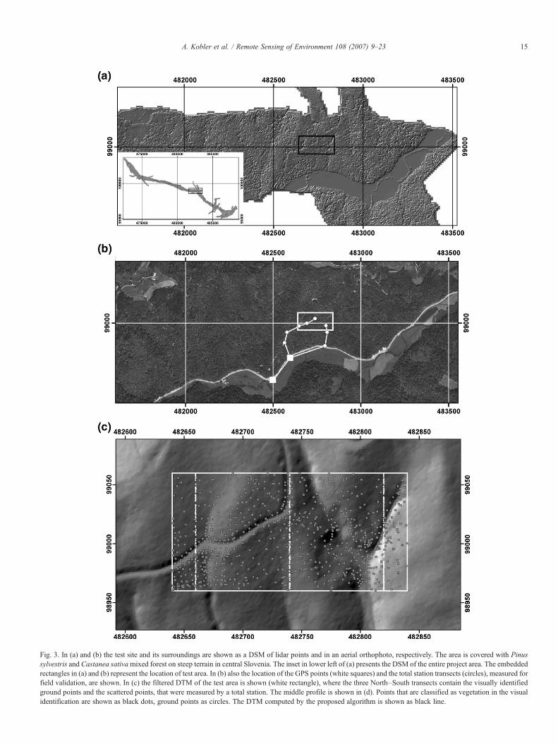
Fig. 3. In (a) and (b) the test site and its surroundings are shown as a DSM of lidar points and in an aerial orthophoto, respectively. The area is covered with Pinussylvestris and Castanea sativamixed forest on steep terrain in central Slovenia. The inset in lower left of (a) presents the DSM of the entire project area. The embeddedrectangles in (a) and (b) represent the location of test area. In (b) also the location of the GPS points (white squares) and the total station transects (circles), measured forfield validation, are shown. In (c) the filtered DTM of the test area is shown (white rectangle), where the three North–South transects contain the visually identifiedground points and the scattered points, that were measured by a total station. The middle profile is shown in (d). Points that are classified as vegetation in the visualidentification are shown as black dots, ground points as circles. The DTM computed by the proposed algorithm is shown as black line.


Fig. 3 (continued ).


datasets are usually massive, using some spatial indexingsetup instead of flat lists of points is important to manage thedatasets efficiently. In our implementation we stored thepoint cloud in the quadtree data structure for efficientpoint indexing (Samet, 1984). The distance ranking method(Hjaltason & Samet, 1995) was used to find the n nearestneighbors in a quadtree. During the initial filtering stage(slope filtering) and during repeated sampling of the initiallyfiltered point cloud, spatial indexing and quick search ofpoints turned out to be essential for ensuring a reasonableprocessing time.

4. Test data and area description

We assessed the performance of the REIN algorithm in atest area of steep forested relief in central Slovenia. Fig. 3ashows a DSM covering a test area of 2 ha, which represents0.17% of the total area scanned (1179 ha). In Fig. 3b anorthophoto of the area is shown. The project area wasscanned for a power line company on April 30, 2003, whenthe vegetation was almost fully developed. From the finalresults (see Section 5) the penetration rate estimated for thelast echoes recorded is 47%.2 The data acquisition was donein the first and last mode with an Optech ALTM 1020scanning Lidar, mounted onto a helicopter. The flying heightwas 260–300 m above the ground, with a ground speed of25–50 km/h, and a beam divergence of 0.3 mrad3. The

2 The selected ground points were used for building a DTM and all pointsless than 0.5 m above that surface are considered to be ground points.3 This, and considering the beam diameter at the aperture, implies a laser

footprint diameter of ∼20 cm, which is lower than typically obtained values of50–100 cm.

obtained point cloud density was 6.4 m−2 and 8.5 m−2 forfirst and last returns, respectively. This value is higher thanobtained by many missions so far4, where a typical density is1 m−2. Only the last returns were used to generate the DTM.While the flying height was rather low, it was counter-weighted by a low pulse repetition frequency (20 kHz) con-sidering that currently available systems offer pulse repetitionfrequency values between 66 kHz and 150 kHz. The spe-cifications of the instrument state that the vertical measure-ment accuracy is ±15cm, and the horizontal accuracy ±35cmin either direction for the given flying height. If the error isonly looked at in the vertical direction, then for a 45° slopethis adds up, by addition of variances, to ±38 cm.

The average terrain slope of the test area was 30°, while theslopes along the forest road embankment and in the erosiondykes reached up to 70°. The test area is covered with a mixedforest with 18 m average tree height, estimated from anormalized digital surface model. The main species are Pinussylvestris and Castanea sativa in the tree layer, and Fagussylvatica and Rhamnus frangula in the forest understorey. In theherbaceous layer Pteridium aquilinum covers half of forestfloor and there is continuous cover of Vaccinium myrtillusunderneath. The average forest canopy cover is 0.67 withextreme values up to 0.86. Canopy cover was estimated forcircular plots (r=5 m) centered at reference ground points as theproportion of first and last lidar returns higher than 1 m aboveground versus all first and last lidar returns.

From the point cloud of last returns, ground points (N=563)for estimation of DTM quality were visually identified within 3

4 However, due the appearance of higher frequency instruments (150 kHz atthe time of writing), equal or higher point densities can be expected in futureapplications.


systematically placed transects oriented in North–Southdirection, each transect being 0.5 m wide and 100 m long(Fig. 3c). To distinguish the ground points each transect wasinteractively rotated. The manual filtering could be seen as thebest possible classification into ground and off-terrain pointsgiven no additional information. Sithole and Vosselman (2004)suggested this method for their comparison of filter algorithms.Practice has shown that filter errors are often obvious tohumans. Correspondingly visual check and correction areroutinely performed by data providers for classification. Asexample, the visual identification within the middle transect isshown in Fig. 3d.

Fig. 4. Comparison of the shaded relief images of the slope filtered baseline DTM (a)DTMs have 1 m by 1 m horizontal resolution. Note the effects of extreme values of Rnumsamples values cause artifacts due to remaining unfiltered vegetation (d, f ). Highsamplesize with moderate numsamples (h) yields marginally better RMSE and save

For overall performance evaluation, a total number of 744field measured ground points (Fig. 3c) were measured with atotal station Leica TC605L. Two points were measured withGPS and from these points transects were established formeasuring ground heights below the canopy cover. Applyingerror propagation, the accuracy of these points is estimated as±5 cm in either coordinate direction. Converting these valuesinto a height error only using a 45° slope as before, the heighterror amounts to ±9 cm.

All the data is projected in the current Slovenian coordinatesystem that is based on the Bessel ellipsoid 1841 and Gauss–Krüger rectangular plane coordinates (conformal, transverse

, morphologicaly filtered DTM (b and c), and results of REIN filtering (d–h). AllEIN parameters: low samplesize values cause relief generalization (d, e) and lownumsamples and high samplesize values yield fewest artifacts (g), however highs computation time.

Fig. 5. (a) Influence of the REIN parameters numsamples and samplesize on thequality of the DTM according to the average RMSE. The average RMSE wasobtained by averaging RMSE values of 50 runs of REIN for each parametercombination. (b) Stability of REIN results as indicated by the standard deviationof RMSE based on 50 runs of REIN for each parameter combination.


cylindrical projection). The projection is Transverse Mercatorwith a central meridian of 15° east, latitude origin 0°, a scalefactor of 0.9999, false easting of +500,000 m, and falsenorthing of −5,000,000 m.

5. Results and discussion

In this section the computation of the DTM is described and anevaluation of the method is performed in several ways. A visualanalysis is performed to check for obvious filter errors or otherartifacts of the algorithm and a comparison to the visually filteredsubset (as described in Section 4) of the original point cloud isperformed. Additionally, the REIN results are compared to theresults of another filter algorithm, and finally, the REIN results arecompared to the field measured ground points. Each of theseevaluations highlights different aspects of the quality assessmentas detailed below. First, however, the computation of the DTM bymeans of REIN and the choice of parameters is described.

5.1. Parameter selection and visual analysis

The visually identified points were used to select the optimalparameters for the DTM computation. The advantage of thisreference data set is, that it is not subjected to georeferencing orcalibration errors, neither from the LRF, Scanner, GPS, and IMUsensor system, nor from errors in the combination of GPS and thetotal station measurements. Also different concepts of the actualground elevation, i.e. top of the herbaceous vegetation, soil–airinterface, or a value in between, measured by different devices doesnot come into play. The only uncertainty stems from the visualinterpretation, but as experience has shown, human operators arereliable in distinguishing between ground and vegetation hits, asdescribed in Section 4.

All the DTM grids generated in this study have a horizontalresolution of 1 m by 1 m. First a baseline DTM was generatedfrom the last returns, by removal of negative outliers from theoriginal point cloud, followed by slope filtering. The optimal kand P values for removing negative outliers were determinedexperimentally and finally set to 10 and 0.2%, respectively. Themean of all average height differences from a point to its 10nearest neighbors amounts to −0.1 m with a standard deviationof ±7 m. The extreme values are, with either sign, 27 m, whichis well above the average tree height (18 m, see Section 4). Theaverage vertical distance from the 0.2% deleted points to their10 nearest neighbors amounts to 17.5 m. With the average tree itcannot be guaranteed, that only negative outliers were removed.Some ground points may have been deleted, provided their 10nearest neighbors are on average 17.5 m higher.

The slope threshold for the initial filter was set to 70°, which isthe steepest slope observed in the test area. This guaranteed thatno ground point was removed from the dataset. Fig. 4a shows thisbaseline DTM. The point density of last returns thus decreasedfrom 8.5 m−2 for all last returns to 4.3 m−2 in the initially filteredpoint set. All the points in the initially filtered point cloud wereused as nodes to build a TIN from which the regular grid DTMwas computed. Using the field-measured ground points thebaseline RMSE is ±0.30 m. However, looking at Fig. 4a it is

apparent that the result is entirely unsatisfactory. Many off-terrainpoints are contained in the ground data set, showing up as smallhills in the shaded relief view. Comparison with the visuallyidentified ground points gives an RMSE of ±0.13 m, which is toooptimistic. The artifacts are not well represented in that figure.The measured field points, on the other hand, are spread moreevenly and show a higher error.

The initially filtered point set is identical with the FPC usedsubsequently by REIN. The quality of the DTM depends onthe values of samplesize and numsamples. The DTM qualityindicator was the global root mean square elevation error(RMSE) using the visually identified points. The influence ofboth parameters on RMSE was determined within the testarea: samplesize was set to values between 1000 and 10,000in steps of 1000 points per hectare, and numsamples was setto 1, 2,…, 10 iterations (see Fig. 4d–h). Since REIN uses

Table 1RMSE values in meters for the filtering with the morphological filtering

Slopeoffilterkernel

RMSE w.r.t.visuallyfiltered groundpoints

RMSE w.r.t.field measuredground points

Average residualw.r.t. fieldmeasured groundpoints

Output numberof groundpoints perhectare

30° 0.34 1.79 −0.96 12,97040° 0.20 0.79 −0.22 28,50650° 0.13 0.41 0.06 35,70860° 0.14 0.28 0.17 38,45570° 0.14 0.30 0.19 39,208REIN 0.16 0.25 0.22 n.a.

The values for REIN (at samplesize=10,000 and numsamples=4) are shown forcomparison.


random sampling of FPCs in each iteration, the resulting DTMfluctuates between individual REIN runs. Therefore 50 runs ofREIN were performed in the test area for each set of REINparameters and the average RMSE values were computed,based on the two sets of ground points — the field-measuredground points and the visually identified ground points. Whilethe RMSE was only computed for the test area itself, duringfiltering a 10 m buffer zone was added around the test area, inorder to exclude the border effects on the performance ofrepetitive TIN interpolation.

For selecting the appropriate parameters an analysis based onthe visually filtered point cloud (N=563) was performed. Thisassessment evaluates filtering accuracy alone, i.e., not takingthe measurement noise of the various components of an air-borne scanning lidar into account. Especially errors of geor-eferencing in the laser data, or any reference data source, do notdistort the assessment of filtering accuracy.

From the 50 REIN based DTMs for each parametercombination the obtained average RMSE values, with referenceto the visually filtered points, range between ±0.16 m and±0.37 m (Fig. 5a). The standard deviation of the RMSE rangesbetween ±3 mm and ±90 mm (Fig. 5b). Fig. 5a shows thatincreasing the samplesize improves the average RMSE,especially at low samplesize values. The lowest RMSE valueof ±16 cm was achieved with a samplesize of 10,000 pointsha−1 taken from the initial FPC, which means that the samplingrate was 23%. Depending on the samplesize REIN needs only 3to 5 iterations (numsamples parameter) to get the optimalRMSE. Further iterations yield a smoother DTM with lessartifacts due to unfiltered vegetation, however, the RMSE startsincreasing slightly (Fig. 4g and h).

Fig. 4 shows the filtering effect of REIN in comparison withthe baseline DTM and with the morphologically filtered DTM.A high level of noise in the baseline DTM (Fig. 4a) and in themorphologically filtered DTM (Fig. 4c) is due to off-groundpoints because of the high slope threshold, which was used inthe slope based filtering and in the morphological filtering.REIN with a very low samplesize value in Fig. 4d and e

Fig. 6. The DTM of the entire scanned area (1179 ha) was produced with REIN, of wshown in Fig. 3a and b, respectively. The small rectangle shows the location of the

(1000 ha−1, corresponding to a sampling rate of 2%) removedall the artifacts seen in Fig. 4a, but caused over-generalization ofrelief features. On the other hand, REIN with a high samplesizevalue in Fig. 4g (10,000 ha−1) removed most artifacts whileretaining the relief detail as can be seen at the valley lines androad embankments. Based on RMSE and on a visual DTMcheck the values of numsamples used in Fig. 4h (i.e., 4) wasfound to be optimal (Fig. 5a) for the respective samplesize valuein the given test area. A low value of numsamples, which seemsto be optimal in the test area, implies a faster processing. On theother hand, larger fluctuations of DTM quality may be expecteddue to the random nature of REIN. Fig. 5b confirms this byshowing a higher standard deviation of RMSE at numsamplesvalues of 4 and lower and samplesize values of 4000 ha−1 andlower. For the test area this leads to the conclusion that theoptimal numsamples and samplesize values considering boththe DTM quality and the expected stability of the DTM qualityare 10,000 ha−1 and 4, respectively. However, near optimalvalues can already be obtained with 7000 points per ha and 3iterations. In an operational setting, the samplesize value for thetest area would be between 4000 ha−1 and 10,000 ha−1,depending on the desired balance between DTM quality andcomputational cost.

hich a subset is shown here, corresponding with the DSM and aerial ortho-phototest area.

5 Overviews on echo detection methods and impacts thereof are discussede.g. in Jutzi and Stilla, 2003; Fox et al., 1993; Hopkinson et al., 2004; Pfeiferet al., 2004.


Analysis based on the field measured ground points yieldsthe same values of numsamples and samplesize for optimalresults, but the average RMSE are approximately 50% larger(Section 5.3). This assures that the transects placement did nothave a large impact on the parameter selection.

No dependence of average RMSE on relief slope and canopycover was found in the test area.

Filtering the area shown in Fig. 3a with REIN results in theDTM shown in Fig. 6. The area comprises flat, moderatelysloped, and steep forested regions as well as regions withoutvegetation. Slopes, including the very steep areas, are main-tained entirely. Also structures such as forest roads and riverembankments are maintained, whereas obvious filter errors areminimal as presented in Fig. 4h.

5.2. Comparison to morphological filtering

The proposed algorithm was compared to the morpholog-ical filtering as specified by Vosselman (2000). The filterkernel was defined with a constant offset of ±53 cm,considering the vertical measurement error of the differenceof two measured elevations, and admissible slopes betweenground points with values of 30° to 70° in steps of 10°. Theseslopes cover the range from the average slope to the extremeslopes in the test area. The filter radius was set to 10 m. Theresulting point clouds were triangulated to produce DTMs. InTable 1 the RMSE values with respect to the visually filteredpoint cloud and the field measured ground points are shown.The number of identified ground points grows strongly forslopes from 30° to 60°, because many ground points in steeperareas are incorrectly removed using too low kernel slopes.Areas of high slopes are essentially chopped off and replacedby (large) triangles of the final TIN (Fig. 4b), which explainsthe negative average residuals for low kernel slopes. Thisartifact vanishes for slopes larger than 70° (Fig. 4c), butvegetation points still remain in the filtered data set. Suchresult is expected, because the morphological filter is ageneral purpose filter, whereas the filter presented here isdesigned for natural, possibly forested, areas and not, e.g., forbuilt-up city areas. The RMSE values are comparable to theresults of REIN and with ±14 cm even slightly lower for themorphological filtering. Fig. 4c, however, shows that thenumber of artifacts, i.e. remaining hills from vegetationpoints, is much higher in the morphological filter results thanin the optimal REIN example. As with the slope filteringresults, the transects of visually identified points apparentlyby-pass most of the artifacts in morphologically filtered DTM.The measured field points, on the other hand, are spread moreevenly and show a higher error for the morphological filteringthan for REIN.

5.3. Assessment of REIN based on the field measured groundpoints

To assess the overall performance of the proposedalgorithm and the given data, the points measured withtotal station were compared to the DTM computed with

REIN and the DTMs obtained from morphological filtering(Table 1).

In Table 1, the parameters chosen for REIN are those asdescribed in Section 5.1, i.e., 10,000 points per ha and 4iterations. These values are not only optimal when comparing tothe visually identified points, but also optimal when comparingto the field measured ground points. For REIN the RMSE is±25 cm (compared to ±16 cm for the check against the visuallyidentified ground points), the extremes are −84 cm and +97 cmand the mean value of the residuals is +21.5 cm, indicating thatthe laser points lie higher than the tachymetrically measuredpoints in this area. This observation is also supported by theanalysis of themorphological filtering (Table 1, column showingaverage residuals).

Possible explanation for the offset within the REINalgorithm is an exceedingly high value of gmo, but as a similarheight shift is also observed for the morphological filter results,this is excluded. Also the removal process for negative outlierscannot explain that upward shift. In fact, the average height ofthe removed points is 15 cm above the DTM computed withREIN, which indicates that the removal process was too strictbecause too many real ground points were removed, too. Com-paring all points, i.e. also those marked as negative outliers, tothe DTM shows that the point with the largest negative distanceto the DTM is 0.91 m below. The 0.2% of points with the largestnegative distances reach up to 45 cm below the terrain, which isin the same order as the precision derived above.

The offset can, however, be explained by the measurementcharacteristics of laser scanning. Over steep ground an upwardshift is observed in the measured points because the echodetection techniques in the receiver favor the rising edge of thebackscattered signal, which is coming from the higher regionwithin the footprint. Also the herbaceous vegetation causes anoffset of the points as the reflection of the laser energy isperformed, at least partly, by the leaves a few cm above theground.5 An error in geo-referencing cannot be excluded, either,but is not necessary for explaining the effect.

Reducing the lidar point elevations by the mean valuereduces the RMSE to ±20 cm for REIN. This value has to besplit into three vertical components: the total station measure-ment accuracy (±9 cm, Section 4), the lidar point accuracy(±38 cm, Section 4), and the ground point selection accuracy(±15 cm, which is the RMSE with reference to the visuallyidentified ground points). Adding these three accuracy figuresquadratically amounts to ±42 cm, which is much higher than theaccuracy of ±20 cm for REIN after subtracting the offset.Obviously, not all of these errors are purely random, i.e.different for each point, which would justify adding themquadratically. Some of these errors are therefore systematic, inthe sense of “similar for neighboring points”. The randomcomponent of the lidar point accuracy may therefore be below ±20 cm within the investigated area.


Summarizing, REIN provides on the sample data a groundpoint classification of ±16 cm (obtained from the comparison tovisual identified ground points) and a DTM accuracy of ±20 cm.

6. Summary and conclusions

We presented the repetitive interpolation (REIN) method forDTM computation from the raw airborne laser scanning pointcloud. It is especially applicable in steep, forested areas whereother filtering algorithms typically have problems distinguish-ing between ground returns and off-ground points reflected inthe vegetation. The REIN algorithm is applied after initialfiltering, which involves the removal of all negative outliers andthe removal of most, but not necessarily all, off-ground points(positive outliers) by some existing filtering algorithm, forinstance the morphological filter. The core idea of the REINalgorithm is to make use of the redundancy in the initiallyfiltered point cloud FPC in order to mitigate the effect of theresidual off-ground points. Multiple independent samples aretaken from the FPC, while each part of the area of interest getsequal probability of being sampled, irrespective of the localground return density. Based on each sample, ground elevationestimates are computed at individual DTM locations, usingsome spatial interpolation method, for instance TIN basedinterpolation. Because the lower bounds of the distributions ofthe elevation estimates at each DTM location are almostinsensitive to positive outliers, the true ground elevations can beapproximated by adding the global mean offset to the lowerbounds of distributions. Assuming that relatively few off-ground points remained in the FPC, the global mean offset canbe estimated over all DTM locations by averaging the offsets ofall elevation estimates to the lower bounds of their respectiveelevation distributions.

The performance of REIN was tested in an area of steep reliefcovered by mixed forest, the influence of sample size and numberof samples (i.e., iterations) on DTM quality was analyzed,and a baseline DTM (i.e., without REIN) and a morphologicalyfiltered DTM were computed for comparison. Using REIN, theobtained global root mean square elevation error values rangedbetween ± 0.16m and ±0.37m, depending on the sample size andnumber of samples. The lowest error of ±0.16 m was achievedwith 4 samples and using a 23% sampling rate. A standardmethodwas applied to the data and the filtering error reached in the bestcase ±3.2 m. Comparison to ground points measured with a totalstation showed a vertical offset of 20 cm, i.e., the lidar points werelying above the ground. Straightforward computation of residualsshowed an overall error of ±0.28 m which includes the maincomponents of laser measurement accuracy and ground pointselection accuracy. Considering the 20 cm offset, the root meansquare error of the lidar DTM computed with REIN, is reduced to±0.20 m.

While REIN uses random sampling to select lidar points ineach iteration, it also ensures that each part of the area of interestgets equal probability of being sampled, irrespective of the localground return density. These properties enable REIN to deal withsparse ground returns under dense forest canopy on one hand,but also with highly redundant ground returns in forest openings

on the other. It results in a homogeneous DTM even under non-homogeneous data input conditions. The problem of negativeoutliers, originating from multi path reflections, is alsoaddressed in the preprocessing step of the REIN method. Therandom sampling makes REIN unique among the methods offiltering airborne laser data. Other filters behave deterministi-cally, always generating a filter error in special situations.Because of its random aspects, these errors do not occur in eachsample taken during REIN and typically cancel out in the finalstep of computing final elevations at the DTM points. REIN hasthus a greater ability to adapt to variations in the terrain.

The final DTM is not biased towards the lowest elevation esti-mates, because the final elevation at each DTM location is com-puted by adding the global mean offset to the lowest elevation ateach DTM location.

REIN does not impose a certain DTM data structure. It canaccommodate either DTM as a regular vector grid or as a TIN. Adata structure that includes break lines is favoured. Concerningbreak lines the presented filter algorithm behaves like otherpresented algorithms, i.e., inducing a small round off. Breaklines should be extracted by a separate process and storedexplicitly. Furthermore, REIN operates by interpolating DTMsfrom several independent samples of lidar points. This enables astraightforward parallelization of REIN, potentially leading to aconsiderable reduction of processing time.

In further work, more complex estimators for the offset, otherthan the mean value could be considered, e.g., by incorporatingadditional knowledge on the influence of low herbaceousvegetation on airborne laser scanning. Further tests of REIN areneeded to get a better assessment of its performance in differentforest types and under various scanning conditions. A new studyat the Slovenian Forestry Institute is studying the influence ofpoint density. In the future we will also concentrate on a methodof automated optimization of REIN parameter values and onapplications of REIN in the forestry domain. As the work hasshown, also the problem of negative outliers, should be studiedfurther. The REIN-based DTM could enable a more accurateDSM normalization in a very steep and eroded terrain, andimplicitly also detailed vegetation height analyses in some geo-morphologically specific habitats, e.g., in narrow karstic dolinesand sinkholes.

Acknowledgements

The authors would like to thank Polona Kalan, SlovenianForestry Institute, and George Sithole, TU Delft, for fruitfuldiscussions of the algorithm. We owe special thanks to ELEScompany, Slovenia, for kindly giving us the lidar data of the testarea. The studywas funded by the Slovenian Research Agency andby the SlovenianMinistry ofAgriculture, Forestry, and Foodwithinthe research project “Processing of Lidar Data” (contract 3311-04-8226575), and by the Slovenian Ministry of Defense and by theSlovenian Research Agency within the research project “Forecast-ing GIS Model of Fire Danger in Natural Environment” (contract3311-04-828032). We are grateful for the support of Prof.Vosselman, ITC Enschede, by providing executables for thestandardmethod of filteringALS data withmorphological filtering.

Appendix A (continued )


Appendix A. The REIN algorithm

#
Inputs: # FPC — list of filtered (3-D) LiDAR points # DTMxy – list of points in the X–Yplane (2-D) we want to include in DTM # num_samples — number of iterations (samples) # sample_size — number of points in each sample # # Output: # DTM— digital terrain model providing elevation for each point in DTMxy # # Time complexity of the algorithm governed by performing Delaunay
triangulation (DT)
# is O(num_samples ⁎ sample_size ⁎ log sample_size)
fun
ction ComputeDTM(FPC, DTMxy, num_samples, sample_size)
# for each point in DTMxy…
foreach (x,y) in DTMxy do EE[x,y] = empty list
# … collect elevations estimated (EE) on different samples taken from FPC
iteration = 1 while iteration b= num_samples do
FPCs = GetSample(FPC, sample_size)
DT = GenerateDT(FPCs) foreach (x,y) in DTMxy do
Zest = ElevationDT(DT, (x,y))
append Zest to EE[x,y]
iteration = iteration +1

# based on elevations calculate global mean offset (gmo)
OS = empty list foreach (x,y) in DTMxy do
offset = Mean(EE[x,y]) — Min(EE[x,y])
append offset to OS
gmo = Mean(OS)

# using estimated elevations and gmo, calculate digital terrain model DTM
DTM = empty list foreach (x,y) in DTMxy do
z = Min(EE[x,y]) + gmo
append (x, y, z) to DTM
return DTM
# Inputs: # FPC — list of filtered LiDAR points # sample_ size — number of points in each sample # # Output: # FSP — list of sample_size randomly selected points from FPC
fu
nction GetSample(FPC, sample_size)
FSP = empty list
while Length(FSP) b sample_size do
(x,y) = random point uniformly distributed over X–Y projectionof FPC
find (x_S,y_S,z_S) in FPC that is closest to (x,y) in the X–Yplane if (x_S,y_S,z_S) not in FSP
append (x_S,y_S,z_S) to FSP
return FSP
#
Input: # P — list of points # # Output: # DT — Delaunay triangulation over the points in P
fun
ction GenerateDT(P)
#
implemented using the Triangle software package available at # http://www-2.cs.cmu.edu/~quake/triangle.html
return DT

#
Input: # DT — Delaunay triangulation # (x,y) — a point # # Output: # zest — estimated elevation of (x,y) according to DT
fun
ction ElevationDT(DT, (x,y))
find triangle T in DT such that (x,y) is within the X–Y projection of T
zest = elevation of the plane defined by T at (x,y) return zest
References

Andersen, H. -E., McGaughey, R., Carson, W., Reutebuch, S., Mercer, B., &
Allan, J. (2004). A comparison of forest canopy models derived from lidarand InSAR data in a pacific northwest conifer forest. International Archivesof Photogrammetry and Remote Sensing, 35(B3) (Istanbul, Turkey).
Axelsson, P. (2000). DEM generation from laser scanner data using adaptiveTIN models. International Archives of Photogrammetry and RemoteSensing, 33(B4/1), 110−117 (Istanbul, Turkey).

Blair, J., Rabine, D., & Hofton, M. (1999). The Laser Vegetation ImagingSensor: A medium-altitude, digitisation-only, airborne laser altimeter formapping vegetation and topography. ISPRS Journal of Photogrammetryand Remote Sensing, 54, 115−122.

Bufton, J. (1989). Laser altimetry measurements from aircraft and spacecraft.Proceedings IEEE, Vol. 70 (pp. 463–477).

Elmqvist, M. (2001). Ground estimation of lasar radar data using activeshape models. OEEPE workshop on airborne laser scanning and interfero-metric SAR for detailed digital elevation models, Stockholm, Sweden.

Fox, C. S., Accetta, J. S., & Shumaker, D. L. (1993). Active electro-opticalsystems, Vol 6, of The infrared and electro-optical system handbook. SPIEOptical Enginnering Press.

Haralick, R. M., & Shapiro, L. G. (1992). Computer and Robot Vision, Vol. I.Reading, MA: Addison Wesley.

Hjaltason, G. R., & Samet, H. (1995). Ranking in spatial databases. InEgenhofer & Herring (Eds.), Lecture notes in computer science, Vol. 951(pp. 83–95). Berlin: Springer-Verlag.

Hopkinson, C., Lim, K., Chasmer, L. E., Treitz, P., Creed, I. F., & Gynan, C.(2004). Wetland grass to plantation forest — Estimating vegetation heightfrom the standard deviation of lidar frequency distributions. InternationalArchives of Photogrammetry and Remote Sensing, 36(8W2), 288−294(Freiburg, Germany).

Hyyppä, J., Hyyppä, H., Litkey, P., Yu, X., Haggrén, H., Rönnholm, P., et al.(2004). Algorithms and methods of airborne laser-scanning for forestmeasurements. International Archives of Photogrammetry and RemoteSensing, 36(8/W2) (Freiburg, Germany).

Ip, A., El-Sheimy, N., & Hutton, J. (2004). Performance analysis of integratedsensor orientation. International Archives of Photogrammetry and RemoteSensing, 35(B5) (Istanbul, Turkey).

Jacobsen, K., & Lohmann, P. (2003). Segmented filtering of laser scannerDSMs. International Archives of Photogrammetry and Remote Sensing, 34(3/W13) (Dresden, Germany).

Jutzi, B., & Stilla, U. (2003). Analysis of laser pulses for gaining surface featuresof urban objects. 2nd GRSS/ISPRS Joint Workshop on Remote Sensing andData Fusion of Urban Objects, URBAN 2003, IEEE (pp. 13−17).

Kaartinen, H., et al. (2005). Accuracy of 3D city models: EuroSDR com-parison. International Archives of Photogrammetry and Remote Sensing,Vol. 36, 3/W19. The Netherlands: Enschede.


Kass, M., Witkin, A., et al. (1988). Snakes: Active contour models. Interna-tional Journal of Computer Vision, 1, 321−331.

Kilian, J., Haala, N., & Englich, M. (1996). Capture and evaluation of airbornelaser data. International Archives of Photogrammetry and Remote Sensing,31(3), 383−388 (Vienna, Austria).

Kraus, K., & Pfeifer, N. (1998). Determination of terrain models in woodedareas with airborne laser scanner data. ISPRS Journal of Photogrammetryand Remote Sensing, 53, 193−203.

Lohmann, P., Koch, A., & Schaeffer, M. (2000). Approaches to the filtering oflaser scanner data. International Archives of Photogrammetry and RemoteSensing, 33(B3/1), 534−541.

Measures, R. M. (1992). Laser remote sensing: Fundamentals and applications.Malabar, Fla: Krieger Pub.

Nardinocchi, C., Forlani, G., & Zingaretti, P. (2003). Classification and filteringof laser data. International Archives of Photogrammetry and RemoteSensing, 34(3W13) (Dresden, Germany).

Pfeifer, N., Gorte, B., & Oude Elberink, S. (2004). Influences of vegetation onlaser altimetry — Analysis and correction approaches. InternationalArchives of Photogrammetry and Remote Sensing, 36(8W2), 283−287(Freiburg, Germany).

Pfeifer, N., Stadler, P., & Briese, C. (2001). Derivation of digital terrain modelsin the SCOP++ environment. OEEPE workshop on airborne laserscanningand interferometric SAR for detailed digital elevation models, Stockholm,Sweden.

Samet, H. (1984). The Quadtree and related hierarchical data structures. ACMComputing Surveys (CSUR), 16/2, 187−260.

Schiewe, J. (2001). Ein regionen-basiertes Verfahren zur Extraktion derGeländeoberfläche aus Digitalen Oberflächen-Modellen. Photogramme-trie, Fernerkundung, Geoinformation, 2, 81−90.

Shewchuk, J. R. (2005). Triangle: A two-dimensional quality mesh generatorand Delaunay triangulator. http://www.cs.cmu.edu/~quake/triangle.html,last accessed September 29, 2005.

Sithole, G. (2001). Filtering of laser altimetry data using a slope adaptive filter.International Archives of Photogrammetry and Remote Sensing, 34(3/W4),203−210 (Annapolis, ML).

Sithole, G. (2005). Segmentation and Classification of Airborne Laser ScannerData, Dissertation, TU Delft, ISBN 90 6132 292 8, Publications on Geodesyof the Netherlands Commission of Geodesy, Vol. 59.

Sithole, G., & Vosselman, G. (2004). Experimental comparison of filteralgorithms for bare—Earth extraction from airborne laser scanning pointclouds. ISPRS Journal of Photogrammetry and Remote Sensing, 59, 85−101.

Sohn, G., & Dowman, I. (2002). Terrain surface reconstruction by the use oftetrahedron model with the MDL criterion. International Archives ofPhotogrammetry and Remote Sensing, 34(3A), 336−344 (Graz, Austria).

von Hansen, W., & Voegtle, T. (1999). Extraktion der Geländeoberfläche ausflugzeuggetragenen Laserscanner-Aufnahmen. Photogrammetrie, Ferner-kundung, Geoinformation, 4, 229−236.

Vosselman, G. (2000). Slope based filtering of laser altimetry data. Interna-tional Archives of Photogrammetry and Remote Sensing, Vol. 33, B3/2(pp. 935–942). The Netherlands: Amsterdam.

Wagner, W., Ullrich, A., Ducic, V., Melzer, T., & Studnicka, N. (2006). Gaussiandecomposition and calibration of a novel small-footprint full-waveformdigitising airborne laser scanner. ISPRS Journal of Photogrammetry andRemote Sensing, 60, 100−112.

Zakšek, K., & Pfeifer, N. (2006). An improved morphological filter for selectingrelief points from a LIDAR point cloud in steep areas with dense vegetation.Technical Report, Institute of Anthropological and Spatial Studies, Solvenia.http://iaps.zrc-sazu.si/files/File/Publikacije/Zaksek_Pfeifer_ImprMF.pdf,accessed 6.6.2006.

Zhang, K., Chen, S., Whitman, D., Shyu, M., Yan, J., & Zhang, C. (2003). Aprogressive morphological filter for removing nonground measurementsfrom airborne LIDAR data. IEEE Transactions on Geoscience and RemoteSensing, 41(4), 872−882.

Zwally, J., et al. (2002). ICESat's laser measurements of polar ice, atmosphere,ocean, and land. Journal of Geodynamics, 34, 405−445.

http://www.cs.cmu.edu/~quake/triangle.html

http://iaps.zrc-azu.si/files/File/Publikacije/Zaksek_Pfeifer_ImprMF.pdf

A robust algorithm for DTM generation from Aerial Laser ...

Documents

Transcript of A robust algorithm for DTM generation from Aerial Laser ...