Tolerance envelopes of planar mechanical parts with

parametric tolerances

Yaron Ostrovsky-Berman and Leo Joskowicz

School of Engineering and Computer Science

The Hebrew University of Jerusalem, Jerusalem 91904, Israel

Email: yaronber@cs.huji.ac.il

Abstract

We present a framework for the systematic study of parametric variation in planar me-chanical parts and for efficiently computing approximations of their tolerance envelopes.Part features are specified by explicit functions defining their position and shape as a func-tion of parameters whose nominal values vary along tolerance intervals. Their toleranceenvelopes model perfect form Least and Most Material Conditions (LMC/MMC). Toleranceenvelopes are useful in many design tasks such as quantifying functional errors, identify-ing unexpected part collisions, and determining device assemblability. We derive geometricproperties of the tolerance envelopes and describe four efficient algorithms for computingfirst-order linear approximations with successive accuracy. The results from experimentson 14 realistic part models demonstrate that on average, our algorithms are an order ofmagnitude faster and more accurate than the commonly used Monte Carlo simulation, andproduce better results than the computationally expensive Taguchi method.

Keywords: tolerancing, parametric models, tolerance zones, mechanical design.

1 Introduction

Manufacturing and assembly processes are inherently imprecise, producing parts that vary insize and form. The need to control the quality of the production and to manufacture partsinterchangeably led to the development of tolerance specifications. Tolerance specifications arethe critical link between the designer and the manufacturer. Designers prefer tight tolerancesto ensure that the part will fit in the assembly and perform its function. Manufacturers, onthe other hand, prefer loose tolerances to lower the production cost and decrease the need forquality machine tools and precision measurement machines. Tolerance analysis methods play akey role in bridging between the two.

Tolerance allocation is difficult even to the most skilled of designers because it requiresidentifying the critical interactions of toleranced dimensions, which often have complex depen-dencies. Tolerancing methods have been developed and incorporated into most modern CADsoftware. Given a tolerance allocation, tolerance analysis consists of predicting the effect ofthe allowed variations on the design functions. Tolerance synthesis consists of finding toleranceintervals that meet the functional requirements at the lowest cost.

A key problem in tolerance analysis is computing the tolerance envelope of a part fromits tolerance specification. Tolerance specifications define a family of parts consisting of allvalid instances of the part. The tolerance zone of a part is the difference between the smallestvolume containing all part instances and the largest volume contained in all part instances.Its boundaries, called the part tolerance envelope, define the worst-case variability of the partfeatures, and thus model perfect form Most and Least Material Conditions (MMC/LMC). Parttolerance zones are useful in design tasks such as quantifying functional errors, identifyingunexpected part collisions, and determining device assemblability.

1

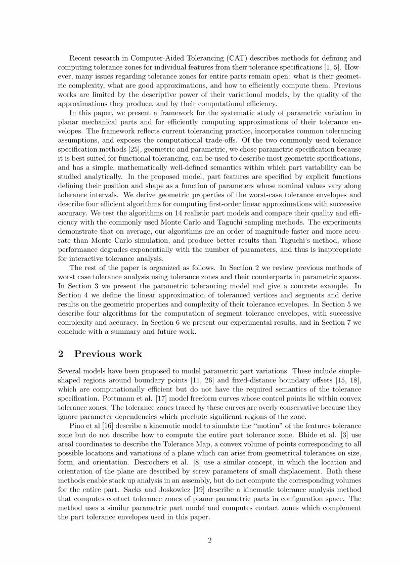
Recent research in Computer-Aided Tolerancing (CAT) describes methods for defining andcomputing tolerance zones for individual features from their tolerance specifications [1, 5]. How-ever, many issues regarding tolerance zones for entire parts remain open: what is their geomet-ric complexity, what are good approximations, and how to efficiently compute them. Previousworks are limited by the descriptive power of their variational models, by the quality of theapproximations they produce, and by their computational efficiency.

In this paper, we present a framework for the systematic study of parametric variation inplanar mechanical parts and for efficiently computing approximations of their tolerance en-velopes. The framework reflects current tolerancing practice, incorporates common tolerancingassumptions, and exposes the computational trade-offs. Of the two commonly used tolerancespecification methods [25], geometric and parametric, we chose parametric specification becauseit is best suited for functional tolerancing, can be used to describe most geometric specifications,and has a simple, mathematically well-defined semantics within which part variability can bestudied analytically. In the proposed model, part features are specified by explicit functionsdefining their position and shape as a function of parameters whose nominal values vary alongtolerance intervals. We derive geometric properties of the worst-case tolerance envelopes anddescribe four efficient algorithms for computing first-order linear approximations with successiveaccuracy. We test the algorithms on 14 realistic part models and compare their quality and effi-ciency with the commonly used Monte Carlo and Taguchi sampling methods. The experimentsdemonstrate that on average, our algorithms are an order of magnitude faster and more accu-rate than Monte Carlo simulation, and produce better results than Taguchi’s method, whoseperformance degrades exponentially with the number of parameters, and thus is inappropriatefor interactive tolerance analysis.

The rest of the paper is organized as follows. In Section 2 we review previous methods ofworst case tolerance analysis using tolerance zones and their counterparts in parametric spaces.In Section 3 we present the parametric tolerancing model and give a concrete example. InSection 4 we define the linear approximation of toleranced vertices and segments and deriveresults on the geometric properties and complexity of their tolerance envelopes. In Section 5 wedescribe four algorithms for the computation of segment tolerance envelopes, with successivecomplexity and accuracy. In Section 6 we present our experimental results, and in Section 7 weconclude with a summary and future work.

2 Previous work

Several models have been proposed to model parametric part variations. These include simple-shaped regions around boundary points [11, 26] and fixed-distance boundary offsets [15, 18],which are computationally efficient but do not have the required semantics of the tolerancespecification. Pottmann et al. [17] model freeform curves whose control points lie within convextolerance zones. The tolerance zones traced by these curves are overly conservative because theyignore parameter dependencies which preclude significant regions of the zone.

Pino et al [16] describe a kinematic model to simulate the “motion” of the features tolerancezone but do not describe how to compute the entire part tolerance zone. Bhide et al. [3] useareal coordinates to describe the Tolerance Map, a convex volume of points corresponding to allpossible locations and variations of a plane which can arise from geometrical tolerances on size,form, and orientation. Desrochers et al. [8] use a similar concept, in which the location andorientation of the plane are described by screw parameters of small displacement. Both thesemethods enable stack up analysis in an assembly, but do not compute the corresponding volumesfor the entire part. Sacks and Joskowicz [19] describe a kinematic tolerance analysis methodthat computes contact tolerance zones of planar parametric parts in configuration space. Themethod uses a similar parametric part model and computes contact zones which complementthe part tolerance envelopes used in this paper.

2

A few CAT packages provide tools for computing worst-case part tolerance zones [22]. Somecompute tolerance zones from many randomly generated part shape instances drawn from apresupposed parameter distribution (the Monte Carlo method) [6], or sample instances of thepart with extremal parameter values (the Taguchi method) [7]. These methods are expensiveand incomplete, as mechanical assemblies typically have hundreds of features defined by tens ofparameters. ADAPT [20], developed by Ford for internal use, computes the tolerance envelopesof parametric planar parts with procedural definitions [13]. It has one procedure for each of themany feature definition cases and incorporates ad-hoc simplifying assumptions that precludequantifying the approximation error. The drawbacks of these methods motivate our work.

3 Tolerancing model

We propose the following tolerancing model for planar parts, which is very general in its seman-tics and has good computational properties.

Let A be a simple planar part whose boundary consists of curved segments. Its nominalshape and variation is defined by an m-dimensional parameter vector p. Each parameter hasa nominal value and a tolerance interval, typically much smaller than the nominal dimension.Formally, the toleranced parametric part model is a 4-tuple A = 〈V, S, p, ∆〉, such that:

• V = {v1(p), v2(p), . . . , vn(p)} is the vertex set, where each vertex vi(p) = (xi(p), yi(p)),1 ≤ i ≤ n, is defined by an explicit standard elementary function of the parameter

vector p = (p1, p2, . . . , pm).

• S = {s1, s2, . . . , sn} is the segment set, where the ith segment is a curve connecting thevertices vi, vi+1, 1 ≤ i ≤ n − 1. Segment sn connects the vertices vn, v1. A curve is aparametric function si : [0, 1] × <m → E2, denoted by si(λ, p). Certain curves dependon additional variables, such as Bezier control points, which are also functions of theparameter vector p.

• p = (p1, p2, . . . , pm) is the nominal parameter vector, where pi is the nominal value ofthe ith parameter, 1 ≤ i ≤ m. The offset vector δ = (δ1, δ2, . . . , δm) of parameter vectorp is the offset from the nominal parameter vector p, that is δi = pi − pi.

• ∆ = {(δ−1 , δ+1 ), (δ−2 , δ+

2 ), . . . , (δ−m, δ+m)} is the tolerancing set, where δ−i and δ+

i are theminimal and maximal allowed variations from the nominal parameter value pi, respec-tively.

The tolerance interval of the ith parameter is the interval: Pi = [pi + δ−i , pi + δ+i ]. The

tolerance interval of the model is an m-dimensional hyperbox defined by the Cartesian productof the intervals: P = P1 × P2 × . . . × Pm. We assume without loss of generality that toleranceintervals are symmetric, i.e. δ+

i ≥ 0 and δ−i = −δ+i . Asymmetric intervals [pi + δ−i , pi + δ+

i ] are

made symmetric by shifting the nominal value to the middle of the interval: pi = pi +δ+i

+δ−i

2 ,

δ+i =

δ+i−δ−

i

2 , δ−i = −δ+i , where pi, δ+

i , and δ−i are the shifted nominal value, maximal andminimal variations, respectively. An instance A(p) of the part model is the part defined by theparameter vector p = (p1, p2, . . . , pm), where pi ∈ Pi, 1 ≤ i ≤ m. Figure 1 shows an example ofa parametric part model of a portion of a sewing machine cover.

The tolerance envelopes of a point v and of a segment s of the part model are the boundariesof the union of all their instances, denoted Ep(A, v) and Es(A, s) respectively. The outer andinner tolerance envelopes of the part, Eo(A) and Ei(A), are the boundaries of the union andthe intersection of all the instances, respectively.

The model can be directly generalized to parts with holes by treating each boundary sep-arately. Note that the proposed model has the same semantics as the standard dimensional

3

��������������� ����������������� ��������� �������������� ��� ������������������ ����� �����������! �����#"������ ����� "$��%�&�'(���*) � +���� +�� �� "$�'$, �����*) � +����������������-"�� +�� �����������!������.)/����� ����� "$��%�&�'(���*) � +������� "$�'$, �.���*) � +�������� ���.���-"�����.0/����� ����� "$��%�&�'(���*) �$� 1��'$, �����*)������2������ � ����

���#��3��546��7 3�898� /�;:��546��7 3�898� �/�=<��#�546��7 >�898� "��=<?:��546��7 >�898���#�@>�3.7 <�A*4=<�A�! /�6:�B.7 >#A*4=<�A�!�/�@3�3.7 C�A*4=<�A�-"��D<�E�7 F.A*4=<�A�*)��@G��A!4=<�A

H ���;F��546��7 :�898H ���3#>I46��7 :�898H ����3��546��7 3�898H "���3��546��7 3�898

J �

J � J J J �

J "

K �

K

K �K!L

M �

M

M �

M "

N��

N. N.�

N�"N.)

N�0

N.2K )

OQPSR�T P�UWV?P�T

XZY�[�\ ]�^�_�`-^#R�^#[aP�T$P�R�V�^#]�bcT�d�P�\ ReT Y�_�P�R�^#]�f�PSV

Figure 1: Tolerance specification of a portion of a sewing machine cover. Vertices v1, . . . , v7 arefunctions of subsets of the 13 parameters: lengths li, angles αi and radii ri. The part on the rightis the nominal part instance defined by the parameter vector (l1, . . . , l4, α1, . . . , α5, r1, . . . , r4).

tolerancing scheme. Conventional tolerance drawings can be translated to the explicit func-tional representation. In the following, we assume that the parameters define geometricallyvalid part instances with the same topology and no self-intersections. When these assumptionsdo not hold, the specification describes physically unrealizable parts with no engineering mean-ing. Such invalid part models must be identified and reported to the engineer, so they canbe fixed. The automatic validation of tolerance specifications is an important topic of currentresearch [14, 24].

4 Tolerance envelope properties

We now present the properties of the tolerance envelopes of individual segments. These formthe basis for efficient computation of the part tolerance envelope.

We define the functions sl, sa, and sb to parameterize line, arc, and Bezier curve segments,respectively. The parameter λ ∈ [0, 1] interpolates between the endpoints v1(p) and v2(p).

sl(λ, p) = (1 − λ)v1(p) + λv2(p) (1)

sa(λ, p) = (1 − λ)v1(p) + λv2(p) + h(λ, p)v⊥12(p) (2)

sb(λ, p) =c−1∑

i=0

Bc−1i (λ)bi(p) (3)

where h(λ, p) =−1+

√

1+4λ tan2 α(p)2

−4λ2 tan2 α(p)2

2 tanα(p)

2

is the height of the triangle defined by v1(p),

v2(p), and the arc point, v⊥12 is the normalized vector perpendicular to v2 − v1, α(p) ≤ π isthe arc angle, {bi(p)}c−1

i=0 are the Bezier control points such that b0(p) ≡ v1(p), bc−1(p) ≡ v2(p),and Bc

i (λ) =(

ci

)

λi(1 − λ)c−i are the Bernstein polynomials. In the following we will slightlyoverload the notation of segments and write s to mean the toleranced segment, s(p) to meanthe instance of s by the parameter vector p, and s(λ, p) to mean a point on the instance s(p)determined by the λ parameter.

4

With today’s manufacturing capabilities, tolerance intervals are usually at least two ordersof magnitude smaller than nominal dimensions. Therefore, we use the standard first-orderapproximation and linearly approximate the vertex and segment functions around the nominalvalues. The linear approximation of vertex vi(p) is defined by:

vi(p) ≈ vi(p) +m

∑

j=1

(

∂vi(p)

∂pj

)

δj (4)

where δj ≡ (pj − pj) is the jth parameter offset and ∂vi(p)∂pj

≡ ∂vi(p)∂pj

|p=p is the partial derivative

of vi(p) by parameter pj evaluated at the nominal parameter value p. Similarly, the linearapproximations of line, arc, and Bezier curve segments are, respectively:

sl(λ, p) ≈ sl(λ, p) +m

∑

j=1

(

(1 − λ)∂v1(p)

∂pj+ λ

∂v2(p)

∂pj

)

δj (5)

sa(λ, p) ≈ sa(λ, p) +m

∑

j=1

(

(1 − λ)∂v1(p)

∂pj+ λ

∂v2(p)

∂pj+

h(λ, p)∂v⊥12(p)

∂pj+

∂h(λ, p)

∂pjv⊥12(p)

)

δj (6)

sb(λ, p) ≈ sb(λ, p) +m

∑

j=1

(

c−1∑

i=0

Bc−1i (λ)

∂bi(p)

∂pj

)

δj (7)

In the rest of this paper we refer to the envelope of the part after the linear approximationas the tolerance envelope, and to the actual envelope as the non-linear tolerance envelope.

A key property of these approximations is that they depend only on the parameters thatdefine the segment coordinates, which are those with non-zero partial derivatives. In complexassemblies, the number of such parameters, ki, is usually much smaller than the total numberof part model parameters m. In the sewing machine cover (Fig. 1), ki ranges from 2 to 9. Inthe following, k is the maximum number of dependent segment parameters.

Consider now the tolerance envelope of a vertex. According to Equation 4, the displacementof v(p) from the nominal point in a given direction d is 〈v(p)− v(p), d〉 = 〈

∑mj=1 ujδj , d〉, where

〈·, ·〉 is the vector inner product and uj ≡ ∂v(p)∂pj

. Thus the maximal displacement of a vertex v

in direction d occurs at extremal parameter offset values δ+j or δ−j . The sign of each parameter

offset depends on the direction d and on the directions of the partial derivatives:

δdj =

δ−j 〈uj , d〉 < 0

δ−j 〈uj , d〉 = 0 and 〈uj , d⊥〉 < 0

δ+j otherwise

(8)

where d⊥ is clockwise perpendicular to d. Note that when the derivative uj is perpendicular tod, we assign an extremal value to δj . This ensures that the offsets determine v(p) uniquely givena direction d. Equation 8 shows that each non-zero partial derivative uj divides the plane intotwo halves separated by a line Lj perpendicular to uj , so that one half gets a maximal offset δ+

j

and the other a minimal offset δ−j . We define Lj as passing through the nominal vertex v(p),and oriented so that the positive offset sign is on its left.

The lines Lj induce a subdivision of the plane into 2k cones, which we call the cone diagram

(Fig. 2a). The parameter offset signs for all directions d within a cone are the same, and define avertex vd(p) = v(p) +

∑mj=1 ujδ

dj which achieves the maximal displacement of v(p) in the cone’s

directions. The chain of vertices defined by vd(p), where d is taken once for each cone, is the

5

g-h�i�j

k�lk�m

k!n

o p/q r�q p�s o p/q p�q p.s

o p�q p�q r s

t�u�v�wSx?ySz-{�wwSz g wv�u i w

| m

}?~�� z g w�{St�u�x

| l| n

�

o�r�q p/q r so�r�q r�q r s

o�r�q r�q p.s�!��� �-����

�5��Q�

�Q� �Q��� �Q�

���

�Q�

�Q����

�-��� �-����

���

�Q� �e�

���

�Q��Q�

���

� ������Q�

�(��� ���S�

� � � �

(a) (b)

Figure 2: The cone diagram. (a) The function v(p) has three non-zero partial derivatives: u1,u2, and u3. These define the cone diagram lines L1, L2, and L3 (dashed), which divide theplane into cones with unique sign vectors (shown with +,− signs). Each sign vector definesparameter offsets that determine an extremal instance of v. The tolerance envelope of v is thesolid convex polygon. (b) Topological events. The cone diagram and the tolerance envelopeof the point are shown before, during, and after the topological event. The top figure showsa switch event, in which two cone diagram lines (L2 and L3) merge before switching position.The bottom figure shows a flip event, in which the line defined by u2 changes orientation as aresult of u2 becoming zero.

tolerance envelope of v(p). The following theorem summarizes the properties of the toleranceenvelope of a point.

Theorem 1. Let A be a toleranced parametric part model and let v(p) be a point on itsboundary with k non-zero partial derivatives. Then the point tolerance envelope Ep(A, v) isthe boundary of a convex, centrally symmetric polygon with at most 2k vertices, and can becomputed in optimal O(k log k) time.

Proof. For each of the parameters pj with non-zero derivative uj , define the segment ξj ≡[ujδ

−

j , ujδ+j ]. Let v(pj) = v(p1, p2, . . . , pj , . . . , pm), that is all parameters but pj are at their

nominal values. Observe that as pj changes from pj + δ−j to pj + δ+j the point v(pj) moves along

the segment ξj translated by v(p), so it traces the set {v(p) + x|x ∈ ξj} which is the Minkowskisum of v(p) and ξj . The Minkowski sum operation is commutative, so the tolerance envelope ofv is the sum of v(p) with all the segments ξj where uj 6= 0. The Minkowski sum of segments is aconvex centrally symmetric polytope called a zonotope [10, 27]. The complexity of a zonotopein the plane is at most twice the number of generating segments, that is 2k. To compute theenvelope, first sort the derivatives according to polar angles, and construct the correspondingcone diagram. Then, choose an arbitrary cone and compute its sign vector and correspondingvertex according to Eq. 8. Compute the next vertices by advancing the cones counter-clockwise,updating the vertex coordinates according to the parameter that inverts its sign. The runningtime is dominated by the sorting operation, which takes O(k log k). The algorithm is optimalbecause the angular sorting problem can be directly reduced to finding the tolerance envelopeof a point.

We now turn to the tolerance envelopes of segments. Conceptually, these are the boundariesof the area swept by the point tolerance envelope as it moves along the nominal segment from one

6

V1(p)- V2(p)-

�-� � �?�� ��  � �?��

V1(p)-

V2(p)-

(a) line segment (b) circular arc (c) Bezier curve

Figure 3: Tolerance envelopes of individual segments. Solid thick curves represent the nominalsegments, solid thin closed curves represent the tolerance envelopes, which bound all the thinpolygons representing instances of point tolerance envelopes along the segment.

¡�¢ ¡�£

¤�¥¦

§

¦©¨ ¦ ¥

ª

«�¬�­�®�¯¤ ¨

°�±�²�³�´

(a) (b)

Figure 4: Proof of monotonicity of the tolerance envelope. (a) case 1: w is a midpoint ofthe segment s(pw); (b) case 2: w is the left endpoint of s(pw). The light gray polygon is thetolerance envelope of v1.

endpoint to another. The sweep defines an arrangement of curves, whose outer cell defines thetolerance envelope (Fig. 3). The tolerance envelope of a point on a nominal segment is computedas for vertices, except that the vectors uj are now functions of λ (the terms in brackets in Eqs. 5,6, and 7). As the point moves between the segment endpoints, its cone diagram lines rotate,thus changing the shape of the tolerance envelope. When the cone diagram lines overlap orchange their orientation, the topology of the diagram (and therefore of the point envelope)changes (Fig. 2b). The following lemmas state important properties of segment envelopes.

Lemma 1. Let s be a segment of the toleranced parametric part model, let v1 and v2 be itstwo endpoints, and let L12 be the line determined by v1(p) and v2(p). Define the up and downdirections to be orthogonal to L12 and the orientation of an instance s(p) to be the direction ofs(0, p)s(1, p) with respect to the L12-axis. If every instance of s is monotonic with respect toL12 and has the same orientation as the nominal segment, then the upper and lower parts ofthe tolerance envelope are L12-monotone.

Proof. By contradiction. Assume that the upper part of the envelope is not monotone andthat the non-monotone section of the envelope points towards the left as illustrated in Figure 4.Then there exist two points on the upper part of the envelope t1, t2 such that a line L orthogonalto L12 intersects both (assume t1 is the lower point). The points define an area T bounded onthe right by L and on the left by the envelope. Let w be the leftmost point on the boundary ofT , and let w1 and w2 be the endpoints of a segment instance s(pw) that intersects w (assumew1 is the left endpoint). Since every instance is L12-monotone, either w1 is to the left of w(and therefore outside of T ) or w1 = w. In the first case (Figure 4a) there must be a point ons(pw) between w1 and w that is outside of the tolerance envelope. But this is a contradiction,because the envelope contains all the instances. In the second case (Figure 4b) there must existtwo additional points r1, r2 that intersect L, otherwise w would be the point dividing the upper

7

and lower parts of the envelope from the left, and t1 would belong to the lower envelope. Thesepoints define a similar area R with q as its leftmost point. Note that q is also an endpoint ofan instance of the segment, s(pq). Since both w and q are left endpoints of instances of s, theyare part of the tolerance envelope of v1. But according to our construction there exists a pointon the segment connecting q to w outside of the envelope, a contradiction to the convexity ofthe point tolerance zone.

Lemma 2. Let s, v1, v2, and L12 be as in Lemma 1, let n be the normalized vector in the

direction of L12, and let u(1)i and u

(2)i denote the partial derivatives by pi of v1 and v2 respectively.

Then every instance of s is L12-monotone and has the same orientation as the nominal segmentif the following conditions hold:

1. If s is a line segment, then∑m

i=1 |〈u(1)i − u

(2)i , n〉δ+

i | < ‖v1(p) − v2(p)‖

2. If s is a circular arc segment with angle α(p), and α12(p) is the angle made by v2(p)−v1(p)and L12, then in addition to condition 1, we require that maxp(α(p)/2 + α12(p)) < π/2.

3. If s is a cubic Bezier curve with control points b1, b2, b3, b4 whose derivatives are

u(1)1 , u

(2)1 ,u

(3)1 , and u

(4)1 respectively, then the nominal segment must be L12-monotone,

and∑m

i=1 |〈u(i1)i − u

(i2)i , n〉δ+

i | < ‖bi1(p)− bi2(p)‖ for each of the following pairs of indices:(i1, i2) ∈ {(1, 2), (1, 3), (1, 4), (2, 4), (3, 4)}. For quadric curves with control points b1, b2, b3

the same condition applies with index set {(1, 2), (1, 3), (2, 3)}.

Proof. In the following we assume without loss of generality that L12 is horizontal in the positivex direction. We divide the proof according to the segment type:

1. Line. Every non-vertical line segment is L12-monotonic. We show that all the instanceshave the same orientation as the nominal segment if and only if the condition holds. Theleft side of the condition sums the maximal contribution of each parameter in advancingv1 and v2 towards each other in the x direction. If the sum is less than the nominalhorizontal distance (the right hand side) then the line segment has the same orientation.If the condition does not hold, then the instance that achieves the maximum has theopposite orientation (or is vertical).

2. Arc. Observe that every arc with angle α > π in not x-monotone. Arcs with smaller anglesare not monotone when the angle of the tangent to the right vertex with the positive x-axis is smaller than 90◦ (Fig. 5). This angle is equal to the sum of the angles α(p)/2 andα12(p) as defined above. A symmetrical condition exists for the tangent to the left vertex.

µ6¶ ·µ ¸ ¶

¸ ·µ�¹$º

»�¼�½

¾(¿�À�Á�Â�À*¾

Figure 5: Monotonicity condition for circular arcs

3. Bezier. Let bix denote the x-coordinate of the ith control point. Then a cubic Bezier curveis x-monotone if b1x < b2x, b3x < b4x, and a quadric curve is x-monotone if b1x < b2x < b3x.This follows from the fact that the derivative of the x-coordinate of the curve is strictlypositive when the control points are thus constrained. The lemma’s conditions ensure that

8

the monotonicity conditions are true for the nominal curve, and by the same argumentas for line segments remain true for every instance of the curve, because b2x, b3x cannotcross the endpoints’ x-coordinate.

From Lemmas 1 and 2 we directly get the following corollary:

Corollary 1. The tolerance envelope of a segment that satisfies the conditions of Lemma 2 isL12-monotone.

In the following, we assume for simplicity of presentation that the toleranced segments satisfythe conditions of Lemma 2, thus their tolerance envelopes are L12-monotone and their upper andlower envelopes are well defined. This assumption holds for most practical applications. Whenit does not hold, the required modification to the algorithms slightly increases the asymptoticcomplexity.

Lemma 3. The tolerance envelope of a line segment sl consists of four parts: two convexpolylines corresponding to the left and right sections of the envelope, and two concave curvescorresponding to the upper and lower sections of the envelope.

Proof. According to Theorem 1, the tolerance zones of the vertices are convex polygons. Theirboundaries correspond to endpoints of the segment’s instances, and contribute to the left andright sections of the tolerance envelope (see Figure 3a). Define the upper (lower) envelope asthe section of the envelope that is disjoint from the tolerance zones of the vertices, and above(below) the nominal segment. We now prove that it is concave. Let Es(A, sl) be the toleranceenvelope of sl, and let q ∈ Es(A, sl) be a point on the upper envelope. Then q is incident onsome line segment instance sl(pq). Let hq be the supporting line of sl(pq), and let h+

q be thehalfspace containing hq and above it. Note that hq is tangent to the envelope at q becauseotherwise there would exist q′ ∈ hq above the upper envelope. Now let H be the set of allsupporting lines of points on the upper envelope. Since each of the lines is tangent to thetolerance envelope, the tolerance envelope is contained in the boundary of the intersection of allthe halfspaces, ∂

⋂

h∈H h+. The intersection is convex, so its boundary is a convex curve. Theupper envelope is a continuous subset of the curve, and therefore convex (in fact it is concavebecause the tolerance zone is below the upper envelope). The proof for the lower envelope issymmetrical.

5 Tolerance envelope computation

We now address the representation and computation of part tolerance envelopes. We are inter-ested in part tolerance envelopes whose segments are as few and as simple as possible, yet areas close as possible to the real boundary. Simple segments follow the perfect form assumption,which stipulates that the tolerance envelope of a segment is a chain of segments of the sametype, and facilitates further analysis and manipulation, such as stack-up tolerance analysis,collision detection, and assembly planning. Fewer segments speed up computation but com-promise accuracy and simplicity, e.g., one long spline curve versus many short line segments.Since different applications will require different trade-offs between shape simplicity, accuracy,and efficiency, we define four successive approximations for segment tolerance envelopes: 1.Independent Parameter Approximation (IPA); 2. Extremal Parameter Approximation (EPA);3. Extremal Vertex Approximation (EVA); and 4. Best Segment Approximation (BSA). Wedescribe them next.

9

5.1 Independent Parameter Approximation (IPA)

When the parameters of the segment control points are independent (i.e. each control pointhas a different set of parameters with non-zero partial derivatives), the control points can varyanywhere within their tolerance zones independently from the other points. This problem wasstudied in [13] for line segments and circular arcs, and in [17] for Bezier curves. The tolerancezone under the independency assumption is a conservative approximation, as it contains thetolerance zone defined by dependent parameters, and thus never underestimates the worst casevariation of the part.

For the case of line segment envelopes, the approximated tolerance zone contains everyline segment connecting points in the two endpoints’ envelopes. Thus the IPA envelope is theboundary of the convex hull of the vertices of the tolerance envelopes of the endpoints. It iscomputed in O(k log k) time by finding the outer tangents of the two polygonal envelopes.

We defer the discussion for the case of circular arcs and Bezier curves to Section 5.4.

5.2 Extremal Parameter Approximation (EPA)

The vertices of the tolerance envelope of the starting endpoint have unique offset vectors thatdefine instances of the toleranced segment. These instances define the starting paths of thevertices in the sweeping of the tolerance envelope described at the end of Section 4. Similarly,the vertices of the tolerance envelope of the other endpoint define the end of the sweep paths.The instances correspond to the starting and ending topology of the tolerance envelope, and ifthere are no additional topological events in between, then the upper and lower envelopes of thearrangement they define is a good approximation to the upper and lower parts of the toleranceenvelope. We find the upper and lower envelopes of the arrangement with a divide-and-conquermethod [12] in O(k log k) time.

5.3 Extremal Vertex Approximation (EVA)

The tolerance envelope defined by the interpolation parameter λ is the boundary of a convexpolygon containing all the points s(λ, p) with p ∈ P. Except for specific values of λ (see below),there is a unique polygon vertex that attains the maximal displacement from the nominal points(λ, p) in the direction d orthogonal to the tangent to the nominal segment at s(λ, p). We callthis vertex an extremal vertex. This vertex has the offset vector of the cone that contains thedirection d, and as we change λ it will trace a path on the instance defined by this offset vector.The offset vector of the extremal vertex changes only when the cone containing d changes. Wecall this an extremal event.

The values of λ at which extremal events occur are solutions to the equation〈ui(λ), d⊥(λ)〉 = 0 (there are O(k) such events). The tolerance envelope polygon in an extremalevent λe has an edge parallel to the tangent at s(λe, p). One endpoint of this edge is the extremalvertex of λ < λe, and the other is the next extremal vertex. Note that because of the symmetryof the point tolerance envelope, there is a symmetrical vertex for each extremal vertex (fromthe other side of the nominal segment). The EVA extends EPA by computing the extremalevents and the instances of segments corresponding to all the extremal vertices along the sweep.It computes the upper and lower envelope of the arrangement defined by these instances. Thecomputation of extremal instances dominates the time complexity of the algorithm, with O(k)arithmetic operations per instance, for a total of O(k2) operations.

5.4 Best Segment Approximation (BSA)

This method computes the tolerance envelope of a segment up to the desired degree of accuracy.For applications that support general algebraic curves, it computes the exact tolerance envelope

10

Ã!Ä

Ã�Å Ã!Ä�Æ

Ã/Å Æ

ÇÈ-É#Ê�Ë�Ì*Í.Î/Ï-Ð�É�Ñ$ÒÉSÓ�Ó�Ñ�Í�È�Ô Õ=É�Ë�Ô�Í.Ï

Ö�×$Ø.ÙÖ�×(Ø.Ú�Ð�Ø.Ù

Û�ÜÛ�Ý

Û�Ü Þ

Û/Ý$Þ

ß?àâá�áSãaä�å�æ�ç!è�éê(ë

(a) endpoints move along lines (b) endpoints move along circular arcs

Figure 6: Sweep of envelope edges between two consecutive topological events.

(after the linear approximation of the segment). The algorithm performs the sweep of thetolerance envelope from one endpoint to the other.

A key issue is the identification of discrete events in which the topology of the cone diagramchanges. The values of λ in which topological changes occur are solutions to the equations〈ui(λ), u⊥

j (λ)〉 = 0 and ui(λ) = 0, where u⊥j (λ) is perpendicular to uj(λ). The first equation

corresponds to two cone diagram lines coinciding. We call this a switch event (Fig. 2b top).The second equation corresponds to a cone diagram line disappearing before changing its orien-tation. We call this a flip event (Fig. 2b bottom). Flip events are degenerate cases that occurfrequently in practice. They are equivalent to k simultaneous switch events, but we treat themseparately for efficiency and robustness. In between topological events, each vertex of the pointenvelope has a constant parameter offset vector, and therefore moves on a curve of the sametype as the nominal segment.

A basic step in the algorithm is to compute the boundary of the area swept by two neigh-boring point envelope vertices (an edge) from one topological event to the next. Figure 6 showsthe area swept by an edge whose endpoints move along the path of line and arc segments. Theboundary consists of a chain of segments of the nominal type and a general curve. The generalcurve is obtained with one of the following methods:

1. Closed form expression. Let s(p) denote the toleranced segment instance with parametervector p, and let pq1 and pq2 denote the parameter vectors of the endpoints of the sweptedge (note that they differ in one parameter sign only). Define the parameter vectorp(ξ) = (1 − ξ)pq1 + ξpq2. Then s(ξ) ≡ s(p(ξ)) defines a 1-parameter family of segments.From the classical theory of envelopes in Differential Geometry [4, 23], the envelope of a1-parameter family of curves is a curve that is tangent at each of its points to some curveof the family. For parametric curves (x(λ, ξ), y(λ, ξ)) it is the solution to the equation∂x∂λ

∂y∂ξ

− ∂x∂ξ

∂y∂λ

= 0.

We solved the equation for the envelopes of the 1-parameter families of curves s(ξ), andobtained expressions of the following form: an hyperbola for a family of line segments,a general quadratic curve for circular arcs, and a rational parametric curve for Beziercurves. To obtain the sweep boundary, we find the intersection of the envelopes with theextremal curves s(0) and s(1).

2. Direct approximation. Each point on the curve is incident on some instance of s(ξ). Bysampling a constant number of instances with ξ ∈ [0, 1] and computing the envelope ofthem, we obtain an approximation of the curve without having to compute it explicitly.

For applications that require perfect form tolerance envelopes, we approximate the swept curveseither directly as in method 2 above, or by sampling a constant number of points on the

11

1. Solve the topological event equations 〈ui(λ), u⊥j (λ)〉 = 0 and ui(λ) = 0 for

consecutive lines Li and Lj in the cone diagram.2. Store the events in a priority queue according to λ values.3. Compute the offset vectors of the starting tolerance envelope and store their

corresponding segment instances.4. While the event queue is not empty, remove an event from the queue.

i. If switch event (λ, i, j)a. Sweep the four edges defined by (i, j) from previous to current λ.b. Flip the signs of the i and j parameter offsets in the two middle cones.c. Solve the topological event equations for the two new pairs of neighboring

lines and insert the events into the queue.ii. If flip event (λ, i)

a. Sweep all the edges from previous to current λ.b. Update all the instances by flipping the ith parameter offset sign.

5. Compute the upper and lower envelopes of the segments from all the sweeps.

Table 1: The Best Segment Approximation (BSA) algorithm of a single segment.

curve. The Douglas-Peucker heuristic [9] minimizes the error in a the simplification of discretecurves. It can be adapted to general continuous curves by using the curve derivatives. In ourimplementation, we approximated the curve with five segments using method 2.

Table 1 summarizes the BSA algorithm. The algorithm starts by calculating topologicalevents in the initial cone diagram and storing the events in a priority queue according to λvalues. It then iterates over the events, computing the upper and lower envelopes of the areaswept by the edges that participate in the current topological event. Switch events involveonly six cones (three symmetrical) which correspond to four edges of the tolerance envelope.After lines Li and Lj switch, they have new neighbors in the cone diagram and the algorithmchecks for new topological events. Flip events affect the entire cone diagram and thereforerequire all the edges to be swept from their previous to the current topological event. Notethat the algorithm iterates over all the topological events with λ ∈ [0, 1] in order, because theevents discovered in step 4.i.c. occur after the event that triggers the check. The final stepcomputes the upper and lower envelopes of all the segments produced by the sweep during step4. The correctness of the algorithm follows from Theorem 1, Equalities 5 − 7, and from theobservations made above. We now analyze the time and space complexity of the algorithm fora single segment.

Let ts and tf denote the number of switch and flip topological events, respectively. Step1 solves O(k) polynomial equations of a bounded degree in O(k) time. Steps 2 and 3 requireO(k log k) time and O(k) space. Step 4 iterates a total of ts + tf times, where queue operationstake O(log(ts+tf )) time. Switch events require O(1) update and edge sweep operations, while aflip events requires O(k) operations, thus step 4 produces t = O(ts +k(1+ tf )) sweep segments,though not all of them contribute to the tolerance envelope. In the worst case, ts = O(k2) andtf = O(k), so t = O(k2), but on average t is much smaller. The computation of the upperand lower envelopes in step 5 takes O(t log t) time [12], and dominates the time complexityof the algorithm. The space complexity of the algorithm is dominated by the combinatorialcomplexity of the segment tolerance envelope, which is O(t).

We return now to the case of independent parameters. Since each of the vectors ui(λ)depends on the partial derivative of one control point only, its size changes as λ varies but itsdirection does not. Thus there are no topological changes in the cone diagram. In fact it remainsthe same for all values of λ. The tolerance envelope in this case consists of O(k) swept edgesbetween the endpoints’ tolerance envelopes. In the IPA algorithm we force this case to occurby treating each control point as if it has its own parameters. Thus if there are c control points

12

Approximation Space Time Conservative

IPA (line) O(n) O(nk log k) yes

IPA (other) O(nk) O(nk log k) yes

EPA O(nk) O(nk log k) no

EVA O(nk) O(nk2) no

BSA O(nk2) O(nk2 log k) yes

Table 2: Properties of the approximation algorithms for a part with n segments of the same type.The actual space and time upper bounds include a multiplicative factor due to the complexityof Davenport-Schinzel sequences [21], which, for all practical cases, can be treated as a smallconstant. For the time complexity, we assume that the intersection of Bezier curves of lowdegree is found in O(1) time.

with at most k non-zero partial derivatives each, then the cone diagram consists of at mostck lines of fixed directions. The envelope is computed as in the BSA algorithm, with specialattention to the degeneracies introduced at the endpoints (where a subset of the parameters getzero weight). Note that in [17] the tolerance zone is represented implicitly by the curvature ofits envelope, while our method provides an explicit representation of the envelope.

5.5 Tolerance envelope of the part

The tolerance envelope of the entire part is computed by merging the tolerance envelopes ofits segments. Consecutive segments have one common vertex, at the envelope of which theirsegment envelopes terminate. When the segment envelope chains do not intersect, we mergethem with vertices on the common vertex envelope. When they do intersect, we find theintersection with a segment intersection algorithm [2] in O(t log t) time, where t is the lengthof both chains, and merge the chains at the intersection point. If there is more than oneintersection then the envelope has a hole or self intersects. In this case the algorithm informsthe user that the part model is invalid and must be fixed.

Table 2 summarizes the computational properties of the approximation algorithms. TheIPA is the least accurate but gives good results when there are no extremal events in thecone diagram. EPA gives tighter results but misses segment instances that may contributeto the envelope when more than one topological event occurs. The EVA improves on EPAat the cost of time complexity by tracking extremal changes without calculating topologicalevents. BSA is the most computationally expensive but gives both accurate and conservativeresults. Let approx(A) denote the area bounded by the outer tolerance envelope produce bythe corresponding approximation of part A, then the relation between the four approximationsis EPA(A) ⊆ EV A(A) ⊆ BSA(A) ⊆ IPA(A). The relation is reversed for the inner toleranceenvelope.

6 Experimental results

We implemented the four algorithms for parts composed of line and arc segments. The imple-mentation was written in C++ with the CGAL library, and run on a 2.4 GHz Pentium 4 with1GB RAM under Windows XP.

To empirically quantify the accuracy of the approximations, we compared them with adense sampling of the non-linear tolerance envelope (the envelope of the part without the linearapproximation). For each sampled point, we compute its parametric function and solve thenon-linear optimization problem consisting of maximizing the offset in the normal direction.For efficiency, we initialize the optimization procedure with the offset vector computed in the

13

no. name n m kmax k tol(mm) time(sec)

1 cover 7 9 9 4 0.33 142

2 handbrake 20 22 7 4 0.36 832

3 axis support 14 19 10 5 0.36 494

4 optical filter 16 17 10 6 0.09 590

5 camera cam 5 5 5 4 0.26 81

6 camera shutter 12 24 12 6 0.51 487

7 geneva driver 12 9 6 4 0.64 152

8 geneva wheel 24 11 6 5 0.40 548

9 pin wheel 28 10 4 4 0.67 721

10 gear driver 7 6 4 3 0.7 106

11 gear follower 16 6 6 5 0.6 300

12 curved link 16 23 7 5 0.3 745

13 long link 34 25 10 6 0.22 1701

14 8 tooth key 26 47 22 13 0.05 2851

Table 3: Model parameters and real envelope computation times. The table lists, for each model,the number of vertices n, the total number of parameters m, the maximal and average number ofnon-zero partial derivatives of a segment kmax and k respectively, the average tolerance intervallength, tol, and the running time of the non-linear optimization algorithm in seconds.

BSA IPA Monte-Carlo

(a) the BSA envelope of the cover (b) detail

Figure 7: (a) A portion of the sewing machine cover tolerance envelope, and; (b) an enlargeddetail of it. Solid thick curves are the nominal part boundary. Dashed, thin solid, and alternatingdashed curves are BSA, IPA, and Monte Carlo envelopes, respectively.

previous sampled point. Our experiments determined that a uniform sampling of 200 points persegment gives satisfactory results. We implemented the optimization algorithm in MATLAB.

Table 3 shows the characteristics of the 14 different models we tested, each with the runningtime of the optimization algorithm. The running times range from 80 seconds to more than45 minutes, much too long for interactive design (the MATLAB profiler shows that 54.5%of the time is spent running built-in optimized C code, so the running time can be cut inhalf at the most). The models and their tolerance envelopes are available in our web site:http://www.cs.huji.ac.il/∼yaronber/Tolerance Envelopes.htm

We compare the results of our algorithms with those produced by the Monte Carlo andTaguchi sampling methods used in most CAT systems (e.g. CATIA, TASys, TolStack). Sam-pling methods repetitively generate valid instances of the part and analyze each part individu-ally. The Monte Carlo method randomly picks parameter values from a uniform distribution,and repeats the simulation a given number of times (we used 100 instances in our experiments).The Taguchi method picks all possible combinations of predetermined extremal values of the

14

0 0.02 0.04 0.060

5

10

15

20

25

30

error (mm)

frequ

ency

(%)

0 0.2 0.4 0.6 0.8 1 1.20

10

20

30

40

error (mm)

frequ

ency

(%)

(a) BSA absolute error (b) Monte Carlo absolute error

0 1 2 3 4 5 60

5

10

15

20

25

30

35

error (%)

frequ

ency

(%)

0 6 12 18 24 30 36 42 48 54 600

5

10

15

20

25

error (%)

frequ

ency

(%)

(c) BSA relative error (d) Monte Carlo relative error

Figure 8: Error distribution of the envelope approximations of the sewing machine cover. Thehorizontal axis is the difference between the distances of the non-linear and approximated en-velopes from the nominal boundary. The vertical axis is the percentage of the envelope with thiserror. The top two graphs show the absolute difference value in millimeters, while the bottomtwo show the relative difference value from the actual distance.

parameters (3 values per parameter), and thus has exponential complexity. To asses the abilityof sampling methods to compute the worst case, we computed the envelope which minimallycontains all the sampled instances and the envelope which is maximally contained in them, andcompared them with the outer and inner envelopes produced by the optimization algorithm.Note that this is faster than the actual process, because we skip the analysis of every sampledinstance.

Figure 7 shows the results of the algorithms on the sewing machine cover. Note that theIPA envelope is too conservative, while the Monte Carlo envelope is too optimistic, missing theinstances that cause extremal offsets from the nominal. Figure 8 shows a detailed comparison ofthe accuracy of the BSA and the Monte Carlo envelopes of the sewing machine cover. Notice theBSA is roughly 10 times more accurate. This characterizes the results of all our experiments,as shown in Tables 4, 5, and 6. The tables summarize the error statistics of the toleranceenvelopes of the proposed algorithms and the sampling methods on the 14 models of Table 3.For each entry, the first three columns show the relative difference (in percentage) between thedistances of the non-linear envelope and the approximated envelope from the nominal boundary(mean, standard deviation, and maximum). The following three columns show the statistics ofthe absolute value of the difference. The last column shows the computation running time (inmilliseconds for our algorithms and in seconds for the sampling methods).

In general, the BSA envelope is the most accurate, followed by EVA and EPA. The IPAenvelope is the least accurate in terms of maximal error, but for many applications (such as

15

model BSA EPArelative(%) value(mm) time relative(%) value(mm) timex σ max x σ max (ms) x σ max x σ max (ms)

1a 1.71 1.30 5.37 0.023 0.019 0.069 406 1.83 2.08 26.8 0.023 0.020 0.093 1721b 3.43 2.61 11.8 0.093 0.077 0.284 401 3.86 4.51 48.2 0.096 0.079 0.343 1731c 0.81 0.60 3.01 0.005 0.004 0.014 411 0.85 0.97 16.8 0.005 0.005 0.029 1792 0.23 0.32 3.91 0.001 0.001 0.013 687 0.23 0.32 3.91 0.001 0.001 0.013 4373 0.52 0.47 2.73 0.007 0.005 0.041 594 5.91 14.6 80.8 0.162 0.478 2.816 3914 1.52 3.56 27.2 0.003 0.006 0.031 1313 2.91 9.37 96.7 0.007 0.044 0.828 5945 2.28 2.28 12.6 0.011 0.011 0.049 500 2.44 2.18 12.6 0.012 0.011 0.049 1726 0.67 0.73 5.17 0.010 0.011 0.078 438 1.82 4.39 42.8 0.039 0.102 0.718 3297 2.07 0.55 3.52 0.026 0.009 0.076 297 1.54 0.92 3.52 0.020 0.014 0.076 1108 1.31 1.12 4.71 0.010 0.007 0.102 829 1.31 1.12 4.71 0.010 0.007 0.102 4539 0.53 0.21 1.37 0.006 0.002 0.025 828 0.56 0.37 4.47 0.007 0.006 0.102 57810 0.71 0.42 1.68 0.005 0.003 0.015 125 0.78 0.63 5.16 0.006 0.007 0.069 9411 0.27 0.50 4.80 0.003 0.006 0.061 1109 0.27 0.50 4.80 0.003 0.006 0.061 54712 0.56 0.77 9.24 0.006 0.018 0.269 844 2.56 8.31 56.7 0.042 0.148 0.931 42213 0.85 1.70 9.85 0.011 0.022 0.173 2453 0.88 1.71 9.85 0.012 0.023 0.173 111014 0.43 0.22 2.30 0.003 0.002 0.021 1891 0.43 0.22 2.30 0.003 0.002 0.021 1531

average 0.97 1.01 6.74 0.008 0.008 0.073 879 1.67 3.33 25.3 0.024 0.062 0.432 495

Table 4: Approximation error statistics of BSA and EPA tolerance envelopes.

assembly planning) its conservative envelope is sufficient for completeness of the analysis.Experiments 1a-1c test the effect of the tolerance interval length on the quality of the en-

velopes. In experiment 1a we used the specification of Figure 1, and in 1b and 1c multiplied anddivided the tolerance intervals by 2, respectively. As expected from our algorithms, the tighterthe tolerances the better the approximation, and vice versa (because of the linear approxima-tion). Note that this is not so in the Monte Carlo method, where the relative error remainsapproximately the same. Also note the mean and standard deviation of the absolute error ofour algorithms are the same order of magnitude as the average tolerance interval squared. Thisis also expected from the linear approximation. In experiments 1d-1f we tested the effect ofthe number of generated instances on the quality of the Monte Carlo envelope. We used 10,1000, and 10000 instances in experiments 1d, 1e, 1f, respectively, and 100 instances in all otherexperiments. Notice that using 100 times more instances only halves the error, hinting at anexponential number of instances needed to achieve good results. Taguchi’s method generatesall the instances with extremal and nominal parameter values, that is 3k instances. These in-clude all the instances used by the EPA and EVA algorithms, but not BSA. As expected, theaccuracy of Taguchi’s method lies between EVA and BSA, but its running time is much toolong for interactive computation except in the simplest of models. The 8-toothed key (example14) requires a tolerance chain specification and has two segments with 22 parameter dependen-cies. Our computer ran out of memory before it could compute the envelope of 322 instances.Tolerance chains this long are not uncommon in realistic specifications.

Figure 9 shows the optical filter (model 4) and part of its tolerance envelope in detail.We interactively changed the tolerance intervals until the envelope of the cavity shown in thedetail was wide enough. Note the overly conservative approximation of the IPA caused by tightdependencies between the arc parameters. This example also demonstrates a rare special casein which the EPA inner envelope has a large error. This can be avoided at no asymptoticcost by including the nominal segment and the instances corresponding to the midpoints of thetolerance envelope edges. However, for most cases the additional cost is not justified.

7 Conclusion

We have presented a framework for modeling parametric variation in planar parts with curvedboundaries and for efficiently computing first-order approximations of their worst-case toler-ance envelopes. Based on the geometric properties of the tolerance envelopes that we derived,

16

model EVA IPArelative(%) value(mm) time relative(%) value(mm) timex σ max x σ max (ms) x σ max x σ max (ms)

1a 1.82 2.08 16.8 0.023 0.020 0.093 174 5.47 17.9 138 0.040 0.074 0.484 2341b 3.86 4.50 48.1 0.096 0.079 0.342 173 8.59 23.5 153 0.134 0.194 1.075 2331c 0.85 0.97 16.8 0.005 0.005 0.029 174 5.08 16.3 132 0.019 0.040 0.230 2342 0.23 0.32 3.91 0.001 0.001 0.013 453 0.65 2.23 20.3 0.003 0.014 0.119 6103 2.95 8.00 48.1 0.055 0.158 0.951 407 12.2 36.7 240 0.184 0.463 2.22 3284 2.91 9.37 96.7 0.007 0.044 0.828 609 19.1 106 1133 0.026 0.100 0.615 6885 2.30 2.26 12.6 0.011 0.011 0.049 188 24.9 21.3 85.7 0.111 0.084 0.322 2356 1.39 3.00 22.2 0.033 0.094 0.718 359 1.20 2.36 24.2 0.024 0.071 0.743 1727 1.54 0.92 3.52 0.020 0.014 0.076 156 43.1 32.5 96.5 0.525 0.376 1.103 1738 1.31 1.12 4.71 0.010 0.007 0.102 453 7.79 9.33 44.6 0.097 0.126 0.570 4849 0.54 0.26 4.47 0.007 0.004 0.102 688 0.52 0.21 1.37 0.006 0.002 0.025 79710 0.74 0.53 5.16 0.006 0.006 0.069 95 0.75 0.40 1.68 0.006 0.003 0.015 12511 0.24 0.38 4.80 0.003 0.005 0.061 594 0.57 1.06 6.14 0.008 0.015 0.088 93712 2.56 8.31 56.7 0.042 0.148 0.931 453 5.83 18.0 155 0.067 0.174 1.175 50013 0.88 1.71 9.85 0.012 0.023 0.173 1172 1.10 1.91 9.85 0.015 0.029 0.173 150014 0.43 0.22 2.30 0.003 0.002 0.021 1500 0.43 0.22 2.30 0.003 0.002 0.021 412

average 1.53 2.74 22.2 0.020 0.038 0.284 521 8.58 18.1 140 0.079 0.110 0.561 514

Table 5: Approximation error statistics of EVA and IPA tolerance envelopes.

model Monte Carlo Taguchirelative(%) value(mm) time relative(%) value(mm) timex σ max x σ max (sec) x σ max x σ max (sec)

1a 16.7 10.9 56.2 0.294 0.274 1.198 1.94 1.73 1.31 5.82 0.028 0.022 0.070 26.21b 16.5 11.8 51.4 0.587 0.593 2.316 1.92 3.43 2.62 11.8 0.093 0.078 0.284 27.21c 18.3 11.2 52.9 0.157 0.135 0.552 1.95 0.82 0.62 3.14 0.005 0.005 0.016 25.21d 39.3 16.7 97.5 0.616 0.426 1.854 0.19 NA1e 10.7 8.93 50.6 0.190 0.197 1.072 18.6 NA1f 8.45 8.70 39.6 0.138 0.153 0.840 215 NA2 12.7 10.2 47.3 0.071 0.080 1.016 5.67 0.23 0.32 3.91 0.001 0.001 0.013 13.73 22.7 15.9 97.9 0.571 0.531 2.525 3.10 1.19 3.01 19.8 0.021 0.064 0.394 3454 19.5 11.2 94.1 0.064 0.066 0.867 4.18 1.84 4.14 27.9 0.004 0.009 0.191 1355 15.8 12.9 84.2 0.084 0.076 0.477 1.36 2.28 2.29 12.6 0.012 0.011 0.049 1.576 23.8 11.6 57.9 0.479 0.394 0.227 2.59 1.22 3.01 20.7 0.030 0.100 0.786 6467 10.5 9.12 47.3 0.149 0.162 0.818 1.66 1.49 0.98 3.52 0.020 0.014 0.076 1.008 15.0 9.96 48.6 0.209 0.202 1.066 5.53 1.31 1.12 4.71 0.010 0.007 0.102 7.019 22.5 9.63 52.3 0.294 0.127 0.974 9.95 0.54 0.24 4.31 0.007 0.004 0.102 4.1110 10.8 10.2 46.7 0.113 0.109 0.476 1.95 0.71 0.42 1.68 0.005 0.003 0.015 0.4711 27.9 9.42 55.2 0.374 0.126 0.824 4.53 0.27 0.50 4.80 0.003 0.006 0.061 13.712 21.7 12.8 56.8 0.258 0.232 2.586 4.91 0.85 1.42 10.8 0.011 0.028 0.285 15.913 29.2 13.8 58.7 0.427 0.402 3.145 9.30 0.86 1.70 9.85 0.012 0.023 0.173 25914 30.3 12.9 59.7 0.228 0.124 0.525 4.64 insufficient resources ∞

average 19.9 11.4 61.6 0.258 0.207 1.194 4.38 1.11 1.57 10.0 0.012 0.022 0.178 113

Table 6: Approximation error statistics of Monte Carlo and Taguchi tolerance envelopes.

we developed four efficient algorithms that trade-off between shape simplicity, accuracy, andefficiency. Their complexity ranges from O(n) space and O(nk log k) time complexity for theIndependent Parameter Approximation, to O(nk2) space and O(nk2 log k) time complexity forthe Best Segment Approximation, where n is the number of boundary segments and k is themaximum number of dependent segment parameters. The algorithms offer clear running time,simplicity, and accuracy advantages over the commonly used Monte Carlo and Taguchi samplingmethods, as demonstrated by our experimental results.

We are currently investigating the use of tolerance envelopes in a variety of mechanicaldesign and assembly planning tasks, including tolerance envelope stack-up in chains of matedparts, assembly planning with tolerance parts, and toleranced configuration space computation[19]. We are also planning to extend the framework to solid models such as triangular meshes.

Acknowledgement: This work was partially supported by grant from the Israeli Ministryof Science and Technology, Grant Number 01-01509.

17

EPA

Monte Carlo

BSAIPA

IPA

BSA+EPA+IPA

(a) (b)

Figure 9: (a) Optical filter nominal part; (b) detail of the tolerance envelopes

References

[1] The American Society of Mechanical Engineers, New York. ASME Y14.5M-1994 Mathe-

matical Definition of Dimensioning and Tolerancing Principles, 1994.

[2] I. J. Balaban. An optimal algorithm for finding segments intersections. In Proc. of the 11th

annual symposium on Computational Geometry, pages 211–219, 1995.

[3] S. Bhide, J. K. Davidson, and J. J. Shah. Areal coordinates: The basis of a mathematicalmodel for geometric tolerances. In Proc. of the 7th CIRP Int. Seminar on Computer-Aided

Tolerancing, pages 35–44, Paris, France, 2001.

[4] V. C. Boltyanskii. Envelopes. Pergamon Press, 1964. Translation from Russion by RobertB. Brown.

[5] A. Clement, A. Riviere, P. Serre, and C. Valade. The TTRS: 13 constraints for Dimension-ing and Tolerancing. In H. A. ElMaraghy, editor, Geometric Design Tolerancing: Theories,

Standards and Applications, pages 122–131. Chapman & Hall, London, 1998.

[6] D. DeDoncker and A. Spencer. Assembly tolerance analysis with simulation and optimiza-tion techniques. SAE Transactions, 96(1):1062–1067, 1987.

[7] J. R. D’Errico and N. A. Zaino Jr. Statistical tolerancing using a modification of Taguchi’smethod. Technometric, 30(4):397–405, 1988.

[8] A. Desrochers, V. Beron, and L. Laperriere. Revisiting screw parameter formulation foraccurate modeling of planar tolerance zones. In Proc. of the 8th CIRP Int. Seminar on

Computer-Aided Tolerancing, pages 239–248, Charlotte, NC, 2003.

[9] D. H. Douglas and T. K. Peucker. Algorithms for the reduction of the number of pointsrequired to represent a digitized line or its caricature. Canadian Cartographer, 10(2):112–122, 1973.

[10] H. Edelsbrunner. Algorithms in Combinatorial Geometry, volume 10 of EATCS Monographs

on Theoretical Computer Science. Springer-Verlag, Heidelberg, West Germany, 1987.

[11] K. Goldberg, J. Chen, M. Overmars, D. Halperin, B. Karl, and Z. Y. Shape tolerance infeeding and fixturing. In P. Agarwal, L. Kavraki, and M. Mason, editors, Robotics, The

Algorithmic Perspective. A.K Peters, The Netherlands, 1998.

18

[12] J. Hershberger. Finding the upper envelope of n line segments in O(n log n) time. Infor-

mation Processing Letters, 33:169–174, 1989.

[13] C. U. Hinze. A Contribution to Optimal Tolerancing in 2-Dimensional Computer Aided

Design. PhD thesis, Johannes Kepler Universitt Linz, 1994.

[14] T. Kandikjan, J. J. Shah, and J. K. Davidson. A mechanism for validating Dimensioningand Tolerancing schemes in CAD systems. Computer Aided Design, 33:721–737, 2001.

[15] J.-C. Latombe, R. Wilson, and F. Cazals. Assembly sequencing with toleranced parts.Computer-aided Design, 29(2):159–174, 1997.

[16] L. Pino, F. Bennis, and C. Fortin. Calculation of virtual and resultant parts for variationalassembly analysis. In Proc. of the 7th CIRP Int. Seminar on Computer-Aided Tolerancing,pages 83–92, Paris, France, 2001.

[17] H. Pottmann, B. Odehnal, M. Peternell, J. Wallner, and R. Ait Haddoi. On optimalTolerancing in Computer-Aided Design. In Geometric Modeling and Processing 2000, pages347–363, Hong Kong, China, 2000.

[18] J. R. Rossignac and A. A. G. Requicha. Offseting operations in solid modelling. Computer

Aided Geometric Design, 3:129–148, 1986.

[19] E. Sacks and L. Joskowicz. Parametric kinematic tolerance analysis of general planarsystems. Computer-Aided Design, 30(9):707–714, 1998.

[20] Schultheiss R., Ford Werke AG, Koln, Germany. ADAPT Users Manual: Computer-Aided

Tolerance Analysis and Design, 2000.

[21] M. Sharir and P. Agarwal. Davenport-Schinzel Sequences and Their Geometric Applica-

tions. New York: Cambridge University Press, 1995.

[22] O. W. Solomons, F. van Houten, and H. Kals. Current status of CAT systems. In Proc. of

the 5th CIRP Int. Seminar on Computer-Aided Tolerancing, Toronto, 1997.

[23] M. Spivak. A Comprehensive Introduction to Differential Geometry. Publish or Perish, 2nd

edition, 1979. In 5 volumes.

[24] N. F. Stewart. Sufficient condition for correct topological form in tolerance specification.Computer Aided Design, 25(1), 1993.

[25] H. Voelcker. A current perspective on Tolerancing and Metrology. Manufacturing Review,6(4):258–268, 1993.

[26] C. K. Yap and E.-C. Chang. Issues in the Metrology of Geometric Tolerancing. In J.-P. Lau-mond and M. Overmars, editors, Algorithms for Robot Motion Planning and Manipulation,pages 393–400, Wellesley, Massachusetts, 1997. A.K. Peters.

[27] G. M. Ziegler. Lectures on Polytopes, volume 152 of Graduate Texts in Mathematics.Springer-Verlag, Heidelberg, 1994.

19