Icing Design Envelopes (14 CFR Parts 25 and 29, Appendix C ...

DOT/FAA/AR-00/30 Office of Aviation Research Washington, D.C. 20591

Icing Design Envelopes (14 CFR Parts 25 and 29, Appendix C) Converted to a Distance-Based Format Richard K. Jeck Federal Aviation Administration Airport and Aircraft Safety Research and Development William J. Hughes Technical Center Atlantic City International Airport, NJ 08405 April 2002 Final Report This document is available to the U.S. public through the National Technical Information Service (NTIS), Springfield, Virginia 22161.

U.S. Department of Transportation Federal Aviation Administration

NOTICE

This document is disseminated under the sponsorship of the U.S. Department of Transportation in the interest of information exchange. The United States Government assumes no liability for the contents or use thereof. The United States Government does not endorse products or manufacturers. Trade or manufacturer's names appear herein solely because they are considered essential to the objective of this report. This document does not constitute FAA certification policy. Consult your local FAA aircraft certification office as to its use. This report is available at the Federal Aviation Administration William J. Hughes Technical Center's Full-Text Technical Reports page: actlibrary.tc.faa.gov in Adobe Acrobat portable document format (PDF).

Technical Report Documentation Page 1. Report No. DOT/FAA/AR-00/30

2. Government Accession No. 3. Recipient's Catalog No.

4. Title and Subtitle

ICING DESIGN ENVELOPES (14 CFR PARTS 25 AND 29, APPENDIX C) 5. Report Date

April 2002 CONVERTED TO A DISTANCE-BASED FORMAT 6. Performing Organization Code

7. Author(s)

Richard K. Jeck

8. Performing Organization Report No.

10. Work Unit No. (TRAIS)

Federal Aviation Administration William J. Hughes Technical Center Airport and Aircraft Safety Research and Development Flight Safety Research Section Atlantic City International Airport, NJ 08405

11. Contract or Grant No.

12. Sponsoring Agency Name and Address

U.S. Department of Transportation Federal Aviation Administration

13. Type of Report and Period Covered

Final Report

Office of Aviation Research Washington, DC 20591

14. Sponsoring Agency Code

ANM-10015. Supplementary Notes

16. Abstract

The conventional liquid water content (LWC) vs mean effective diameter envelopes in Appendix C of 14 CFR Parts 25 and 29 can be redrawn in an equivalent, more versatile form of LWC vs horizontal extent. This document shows how that is done, and it illustrates a number of advantages and uses of this new, distance-based format for the envelopes. 17. Key Words

Aircraft icing, FAR Part 25, Appendix C, Icing design envelopes

18. Distribution Statement

This document is available to the public through the National Technical Information Service (NTIS) Springfield, Virginia 22161.

19. Security Classif. (of this report)

Unclassified

20. Security Classif. (of this page)

Unclassified

21. No. of Pages

55 22. Price

Form DOT F1700.7 (8-72) Reproduction of completed page authorized

iii

TABLE OF CONTENTS Page EXECUTIVE SUMMARY vii 1. INTRODUCTION 1

1.1 Background on Appendix C of 14 CFR Part 25 1 1.2 Using Appendix C of 14 CFR Part 25 5

1.2.1 Selecting Exposure Distances 5 1.2.2 Selecting Values of MVD 5 1.2.3 Difficulties Comparing With Test Data 6

2. CONVERTING APPENDIX C OF 14 CFR PART 25 TO DISTANCE-BASED

ENVELOPES 6

2.1 Conversion Procedure 6 2.2 Uses and Advantages of the Equivalent, Distance-Based Envelopes 10

2.2.1 Selecting Design Points 10 2.2.2 Plotting Data Points 15 2.2.3 Graphing Flight Data 16 2.2.4 Comparing Test Data With the Envelopes 18

2.3 Other Ways to Document Test Data and Compare With Appendix C of

14 CFR Part 25 20

2.3.1 Converting Appendix C of 14 CFR Part 25 to Time-Based Envelopes 20

2.3.2 Converting Appendix C of 14 CFR Part 25 to Water Catch Rate (WCR) Envelopes 22

2.3.3 Converting Appendix C 14 CFR Part 25 to Total Water Catch

(TWC) Envelopes 24

2.3.4 Converting Appendix C of 14 CFR Part 25 to Icing Severity (Intensity) Envelopes 27

2.3.5 Using an Icing Rate Meter to Document Test Exposures 31

3. COMPARING TEST DATA WITH NATURAL PROBABILITIES 35

3.1 The Differences Between Appendix C of 14 CFR PART 25 and Nature 35 3.2 Comparing With Natural LWC Probabilities 36

iv

3.2.1 Icing Wind Tunnel Tests 36 3.2.2 Natural Icing Flight Tests 37

3.3 Comparing With the Natural Altitude Dependence of LWC 38 3.4 Comparing With the Natural MVD Dependence 42 3.5 Comparing With Natural Horizontal Extents 43 3.6 Converting Natural LWC Probabilities to Other Variables 44

4. SUMMARY 45

5. REFERENCES 46

LIST OF FIGURES Figure Page 1 Continuous Maximum (Stratiform Clouds) Atmospheric Icing Conditions (Liquid

Water Content vs Mean Effective Drop Diameter) 2

2 Continuous Maximum (Stratiform Clouds) Atmospheric Icing Conditions (Ambient Temperature vs Pressure Altitude) 2

3 Continuous Maximum (Stratiform Clouds) Atmospheric Icing Conditions (Liquid Water Content Factor vs Cloud Horizontal Extent) 3

4 Intermittent Maximum (Cumuliform Clouds) Atmospheric Icing Conditions (Liquid Water Content vs Mean Effective Drop Diameter) 3

5 Intermittent Maximum (Cumuliform Clouds) Atmospheric Icing Conditions (Ambient Temperature vs Pressure Altitude) 4

6 Intermittent Maximum (Cumuliform Clouds) Atmospheric Icing Conditions (Variation of Liquid Water Content Factor With Cloud Horizontal Extent) 4

7 Appendix C Envelopes Converted to a Distance-Based Format (For MVD = 15 mm) (Logarithmic HE Scale) 11

8a Continuous Maximum, Appendix C, Envelopes for MVD = 15 µm 12

8b Continuous Maximum, Appendix C, Envelopes for MVD = 20 µm 12

8c Continuous Maximum, Appendix C, Envelopes for MVD = 25 µm 13

8d Continuous Maximum, Appendix C, Envelopes for MVD = 30 µm 13

v

9 Intermittent Maximum, Appendix C, Envelopes for Typical MVDs (20 µm) in Convective Clouds 14

10 Continuous Maximum, Appendix C, for Icing Conditions Near 0°C 14

11 Intermittent Maximum, Appendix C, for Icing Conditions Near 0°C 15

12 The Entire Supercooled Cloud Database 16

13 Time Plot of Sample Flight Data (LWC) 17

14 Distance Plot of Sample Flight Data (LWC) 17

15a Sample Flight Data (Cloud Gaps Removed) Compared With Continuous Maximum, Appendix C 19

15b Sample Flight Data (Cloud Gaps Removed) Compared With Continuous Maximum, Appendix C, for Icing Conditions Near 0°C 19

16a Conventional Continuous Maximum, Appendix C With Example Test Points 21 16b Time-Based, Continuous Maximum, Appendix C Envelopes for MVD = 20 µm and

an Airspeed of 174 kt (200 mph) 21 17 Water Catch Rate (WCR) for Sample Exposure (Cloud Gap Removed) Compared

With Continuous Maximum, Appendix C, Converted to WCR Envelopes 23

18 Total Water Catch (TWC) for Sample Exposure (Cloud Gap Removed) Compared With Continuous Maximum, Appendix C, Converted to TWC Envelopes 26

19a Distance Plot of Sample Flight Data (LWC) 28

19b Icing Rate for Sample Exposure 28

20 Continuous Maximum, Appendix C, Converted to Icing Intensity Envelopes 30

21 Sample Icing Intensity (Cloud Gap Removed) Compared With Continuous Maximum, Appendix C, Converted to Icing Intensity Envelopes 31

22a Example of the Rosemount Model 871-FA Analog Output Voltage During a Passage Through Natural Icing Conditions 33

22b Appendix C (Continuous Maximum) in Terms of Icing Rate on a 1/4-inch Diameter Cylinder at 100 kt TAS 33

22c Appendix C (Continuous Maximum) in Terms of Icing Rate on a 1/4-inch Diameter Cylinder at 150 kt TAS in a Distance-Based Format 34

vi

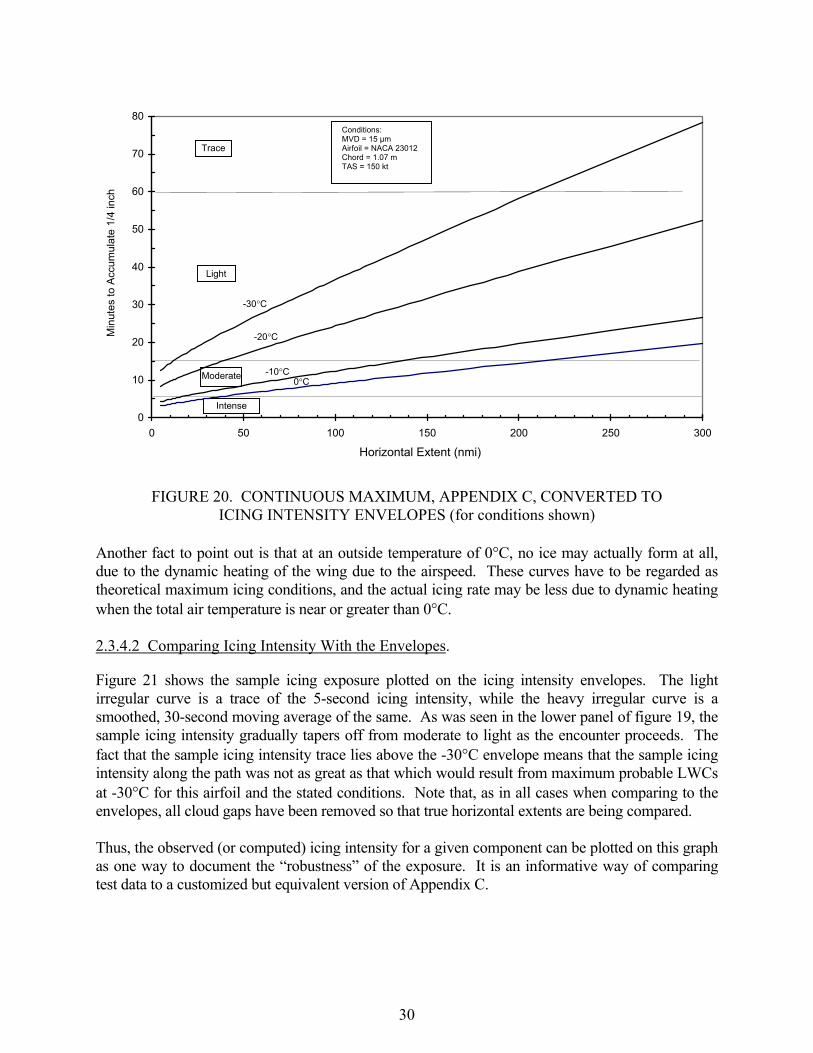
23 Sample Flight Data (LWC) Compared With Natural Probabilities for LWC Averages in Stratiform Icing Conditions With Average MVDs (15 µm) at 0° to -10°C 37

24 Natural 99% LWC Limits vs Altitude (AGL) for Highest Temperatures Available at the Altitude and for all Supercooled Clouds at 15-20 µm MVD 38

25a Natural Probabilities for LWC Averages at Altitudes up to 2500 ft AGL 39

25b Natural Probabilities for LWC Averages at Altitudes of 5000 ft ±2500 ft AGL 39

25c Natural Probabilities for LWC Averages at Altitudes of 10,000 ft ±2500 ft AGL 40

25d Natural Probabilities for LWC Averages at Altitudes of 15,000 ft ±2500 ft AGL 40

25e Natural Probabilities for LWC Averages at Altitudes of 20,000 ft ±2500 ft AGL 41

26 Sample Flight Data (Cloud Gap Removed) Compared With Natural Probablilties for LWC Averages at Altitudes up to 2500 ft AGL 41

27 Natural HE Limits and 99% LWC Limits for Selected, Sustained MVDs in Stratiform Clouds at 0° to -10°C 42

28 Sample Flight Data (Cloud Gap Removed) Compared With Natural 99% LWC Limits for Different MVDs 43

29 Natural Probabilities for Icing Rates on a 1/4-inch Cylinder at 150 kt in Stratiform Icing Conditions With Average MVDs (15 µm) and In-Cloud Temperatures of 0° to -10°C 45

LIST OF TABLES Table Page 1 Intermittent Maximum LWCs Converted to Distance-Adjusted Values 8

2 Continuous Maximum LWCs Converted to Distance-Adjusted Values 9

3 Liquid Water Content Adjustment Factors for Converting Basic LWC Curves (for 15 µm MVD) to LWC Curves for Other MVDs in Distance-Based Appendix C Envelopes 10

4 Durations of Icing Encounters 44

vii/viii

EXECUTIVE SUMMARY This report shows how to convert the conventional liquid water content (LWC) vs mean effective diameter (MED) design envelopes in Appendix C of 14 CFR Part 25 and 14 CFR Part 29 to equivalent, but more useful envelopes based on a LWC vs horizontal extent (HE) format. A number of potential uses are illustrated for the new format, particularly for comparing icing test exposures to the Appendix C envelopes and to natural probabilities of occurrence. The LWC vs HE envelopes can also be recast into envelopes for any other LWC-related variable, such as icing rate or water catch rate, total water catch, and icing intensity, for example. In addition to the Appendix C design envelopes and their derivatives, envelopes are also presented which depict naturally occurring probabilities (99.9%, 99%, 95%, 90%, and 50%) of LWC and the dependence of these probabilities on median volume diameter (MVD), temperature, altitude, and even on the season of the year. These can all serve for comparing icing test exposures from natural icing flights, icing wind tunnels, airborne spray tankers, and computer simulations to the design envelopes of Appendix C and to real world statistics for naturally occurring icing conditions. The methods illustrated here provide the icing practitioner with straightforward, understandable, and meaningful ways to document, compare, and evaluate data on icing conditions. They offer a set of working standards for achieving consistency and uniformity among users. Some methods may be more useful than others, depending on the application, but a variety are offered, with examples, to illustrate the possibilities. The examples also illustrate the use of computerized spreadsheet software for graphing icing variables and for conveniently adjusting or converting the Appendix C envelopes to fit particular applications. This adds new, modern versatility to the envelopes that is not possible with the conventional printed (fixed) version.

1

1. INTRODUCTION.

1.1 BACKGROUND ON APPENDIX C OF 14 CFR PART 25.

This report concerns the set of six figures published in Appendix C of Part 25 (Airworthiness Standards: Transport Category Airplanes) and in Part 29 (Airworthiness Standards: Transport Category Rotorcraft) of Title 14 (Aeronautics and Space) in the U.S. Code of Federal Regulations (14 CFR 25, and 14 CFR 29), (see reference 1). Parts 1-199 of Title 14 are sometimes known as a Federal Aviation Regulation (FAR), and therefore Parts 25 and 29 are sometimes designated FARs 25 and 29. This Appendix C of 14 CFR Part 25 has been in use since 1964 for selecting values of icing-related cloud variables for the design of in-flight ice protection systems for aircraft. The six figures are reproduced here as figures 1 to 6 of this report. Figures 1 to 3 are known as �continuous maximum� conditions and they represent a portion of stratiform icing conditions or layer-type clouds that, in 1964, were considered to be important for the design of thermal ice protection systems on large airplanes. Figures 4 to 6 are known as �intermittent maximum� conditions, and they represent a portion of convective, or cumuliform, clouds and icing conditions. Traditionally, continuous maximum conditions have been applied to airframe ice protection and intermittent maximum conditions have been applied to engine ice protection. These are design envelopes as opposed to more complete scientific �characterizations.� The former contain only those ranges of variables that are thought to be important for the design of aircraft ice protection systems. A complete characterization will require a wider range of variables and values. Figures 1 and 4 are supposed to indicate the �probable maximum� (99%) value of cloud water concentration (usually known as �liquid water content� (LWC)) that is to be expected as an average over a specified reference distance, for a given temperature and representative droplet size in the cloud. For figure 1 this reference or �standard� distance is 20 statute miles (17.4 nmi) in stratiform icing conditions, and for figure 4, it is 3 statute miles (2.6 nmi) in convective icing conditions. These are arbitrary reference distances but were convenient for the original National Advisory Committee for Aeronautics (NACA) researchers in the late 1940s because most of their rotating cylinder measurements were averages over approximately 10 and 3 miles, respectively. These probable maximum values of LWC were estimated by the NACA and Weather Bureau researchers in the early 1950s when they first formulated the basis for the present-day Appendix C [2, 3]. In these icing applications, the actual droplet size distribution (typically 1-30 µm) in clouds is represented by a single variable called the droplet median volume diameter (MVD) or, in the older usage, an approximately equivalent variable called the mean effective diameter (MED). The MVD is the midpoint of the LWC distribution over the range of cloud droplet sizes that happen to be present at the time. The MVD therefore varies with the number of droplets in each size category, but the overall average for layer clouds is about 15 µm while for convective clouds it is about 19 µm. The MVD has proven useful as a simple substitute for the actual droplet size distributions in ice accretion computations.

2

FIGURE 1. CONTINUOUS MAXIMUM (STRATIFORM CLOUDS) ATMOSPHERIC

ICING CONDITIONS (Liquid water content vs mean effective drop diameter)


ICING CONDITIONS (Ambient temperature vs pressure altitude)

3


ICING CONDITIONS (Liquid water content factor vs cloud horizontal extent)

FIGURE 4. INTERMITTENT MAXIMUM (CUMULIFORM CLOUDS) ATMOSPHERIC

ICING CONDITIONS (Liquid water content vs mean effective drop diameter)

4

FIGURE 5. INTERMITTENT MAXIMUM (CUMULIFORM CLOUDS) ATMOSPHERIC

ICING CONDITIONS (Ambient temperature vs pressure altitude)

FIGURE 6. INTERMITTENT MAXIMUM (CUMULIFORM CLOUDS) ATMOSPHERIC ICING CONDITIONS (Variation of liquid water content factor with cloud horizontal extent)

5

1.2 USING APPENDIX C OF 14 CFR PART 25.

Although at this writing there is no comprehensive guide to the use, interpretation, and application of Appendix C, design engineers typically select a conventionally recommended droplet MVD and a temperature appropriate to the flight level of concern, and then use them to obtain the probable maximum LWC from figure 1 or 4 of Appendix C. Other suggested or conventional practices are contained in references [4-9]. 1.2.1 Selecting Exposure Distances.

The values of LWC obtained directly from figure 1 or 4 are valid only for the reference distances of 17.4 nmi or 2.6 nmi, respectively. These were recommended by NACA researchers [2] as �appropriate� design distances for ice protection considerations. If there is some reason to design for a longer (or shorter) exposure distance, then the LWC originally selected may be reduced (or increased) for some applications by a factor obtained from figure 3 or 6 in Appendix C. This is because for both types of clouds, longer averaging distances will result in lower maximum values of LWC as an average over the total exposure distance. To account for this behavior, adjustment factors (figures 3 and 6) had to be developed so the envelopes could be adapted to other averaging distances. For example, to find the maximum probable LWC to be expected as an average during flight through 100 nmi of stratiform icing clouds, the appropriate multiplying factor (0.46 in this example) is taken from figure 3. Thus, for stratiform clouds in which the MVD is 15 µm and the temperature is -10°C (+14°F), the maximum average LWC over 100 nmi is expected to be 0.46 x 0.6 g/m3 = 0.28 g/m3. Basically, this procedure amounts to raising or lowering the LWC curves in figure 1 or 4, depending on the exposure distance. Note that this adjustment of LWC values is the only valid use of the LWC adjustment factor curves (figures 3 or 6). Any other use of the LWC-factor curves is incorrect. The choice of exposure distance depends on the application at hand. One common application is to estimate ice buildup amounts on unprotected surfaces during a long exposure of perhaps 100 or 200 miles [4]. In this case, the LWC obtained from figure 1 is customarily reduced by an amount obtained from figure 3 for the selected exposure distance. Another application is to estimate ice buildups on unprotected surfaces during a 45-minute hold situation. In this case, the LWC obtained from figure 1 is used at full value without any reduction [5]. It assumes the worst case in which the holding pattern happens to be entirely within a 17.4 nmi region of cloudiness containing the maximum probable LWC. 1.2.2 Selecting Values of MVD.

Current practice [4-8] arbitrarily uses an absolute droplet diameter (not an MVD) of 40 microns (µm) for computing the impingement limits of droplets (chordwise extent of ice accretion) on an airfoil. For this purpose, the exposure distance is considered to be irrelevant and none is quoted.

6

Convention has also established the use of a 20 µm MVD for the computation of ice accretion amounts in general, whether for standard exposure distances of 17.4 nmi or longer. Although 20 µm is typically selected for computing ice accretion rates or amounts, reference 4 recommends that �the entire range of (MVD) values should be considered.� This means that the designer is advised to consider exposures to droplets with an MVD up to 40 µm over distances up to 17.4 nmi at least. 1.2.3 Difficulties Comparing With Test Data.

Users often wish to plot on figure 1 or 4 the points representing combinations of LWC, MVD, and temperature that were used in wet wind tunnel tests, computer simulations, test flights behind airborne spray tankers, and test flights in natural icing conditions. Unfortunately, the LWC vs MVD versions of the envelopes (figures 1 and 4) are not well suited for this purpose. The problem is that they are valid only for the fixed averaging distances of 2.6 nmi for convective (intermittent) clouds and 17.4 nmi for stratiform (continuous) clouds. Any LWC data that has been averaged over some other distance cannot be validly plotted on these envelopes without first converting the measurements to a 2.6 or 17.4 nmi average or rescaling the envelopes to agree with the actual averaging distance. Despite attempts by users to convert LWC measurements to an equivalent value over the reference distances, there are major difficulties in doing this legitimately. The only entirely correct procedure is to raise or lower the LWC curves to agree with the actual averaging distance, as described in the preceding section. If the actual test exposure and overall averaging distance is 50 nmi, for example, then the LWC curves for the continuous maximum envelopes must be lowered to about 66% of the original values, according to the F-factor curve in figure 3. The data point can then be validly plotted on the envelopes. Otherwise, the data point would be compared to envelopes that are valid for another averaging interval (horizontal extent (HE)). If other data points are averaged over other distances, the LWC curves in figure 1 or 4 must be adjusted differently for each data point. That is, the data points cannot be legitimately plotted on the same LWC vs MVD envelope unless they are all for the same averaging distance. This limitation appears to be unrecognized or overlooked by many icing practitioners. Needless to say, this is a cumbersome situation. It makes the practical comparison of data points difficult, if not impossible. A better way is to convert figures 1 and 4 to equivalent, distance-based envelopes where the LWC curves have already been adjusted for the distance effect. 2. CONVERTING APPENDIX C OF 14 CFR PART 25 TO DISTANCE-BASED ENVELOPES.

2.1 CONVERSION PROCEDURE.

The conventional Appendix C envelopes treat LWC and MVD as principal variables with exposure distance treated as a constant. For comparison with test data, it is better to treat distance as the true

7

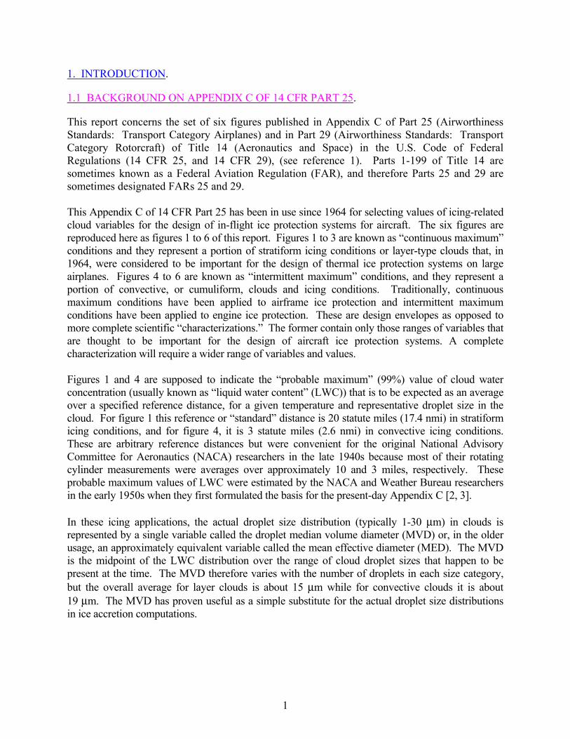
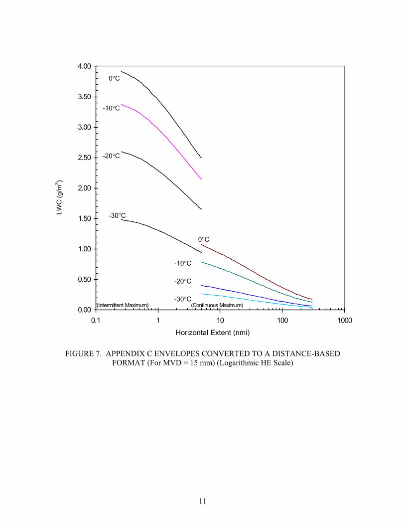
variable that it is, and draw envelopes for fixed values of MVD. In nature, MVDs are much less variable than may be generally realized1. Fortunately, figures 1 and 4 can be easily converted to an equivalent, LWC vs HE format, which easily overcomes the aforementioned limitations. Test points can then be plotted directly on the figures, no matter what the HE or averaging distance. In addition, the LWC adjustment curves (figures 3 and 6) are no longer needed and may, therefore, be eliminated. Moreover, figures 1 and 4 can be combined into a single chart covering both short (intermittent) and long (continuous) horizontal extents. As a result, Appendix C can be reduced from six to only three figuresone for the LWC vs HE envelopes and the two original temperature vs altitude envelopes in figures 2 and 5. The conversion is accomplished simply by taking the LWC values for each major temperature and MVD increment in figures 1 and 4 and multiplying those LWCs by the appropriate F-factor value for a few horizontal extents over the applicable range. The resulting, distance-adjusted LWC values are listed in tables 1 and 2. These adjusted LWC values are then plotted vs horizontal extent to give a string of points for each row in tables 1 and 2. The points in each string are connected by a smooth curve to give a new, but equivalent set of envelopes2. Figure 7 shows the basic set, drawn for the familiar 10°C temperature intervals. In this basic set, not all curves are shown, but only those for MVDs of 15 µm. In this figure, a logarithmic HE scale nicely accommodates both the short HEs of the intermittent maximum envelopes and the long HEs of the continuous maximum curves. Other variations are possible, such as figures 8 and 9 which show the envelopes separately on a magnified, linear HE scale. Figures 8 and 9 emphasize the variation of design3 values of LWC on flight level temperature and exposure distance for typical values of MVD (around 15 µm for stratiform clouds and around 20 µm for convective clouds). Alternately, figures 10 and 11 emphasize the variation of the design values of LWC on MVD and exposure distance, as represented by the current design envelopes, when the flight level temperature is near 0°C. For manual graphing, the basic set of curves in figures 7 to 9 can be adjusted to values appropriate for MVDs other than 15 µm by using the set of adjustment factors given in table 3. Alternately, one can plot all the values given in table 1 or 2 and obtain a complete set of curves for all major temperature and MVD increments. This results in a rather crowded graph and is unnecessary since most of the MVDs other than 15 µm or 20 µm are seldom used anyway. For simplicity, spreadsheet

1 Statistics compiled at the FAA William J. Hughes Technical Center from 10,000 nmi of measurements in stratiform icing conditions reveals that about 75% of all MVDs are within ±5 µm of 15 µm in stratiform clouds. 2 In this report, most of the figures showing the new envelopes have been produced by the charting capabilities of computerized spreadsheet software after entering the data in table 1 or 2 into the spreadsheet. In this way, variations or customized versions of the envelopes can be easily generated. 3 The natural variation of the 99% maximum LWC with HE is somewhat different, depending on the temperature, and especially on the MVD (see figures 22, 24, and 26).

8

charts of selected MVD rows from table 1 or 2 or the use of table 3 is recommended for those occasions where some other than a nonconventional MVD is of interest.

TABLE 1. INTERMITTENT MAXIMUM LWCs CONVERTED TO DISTANCE-ADJUSTED VALUES

MVD HE = 0.26 nmi 0.5 nmi 1.0 nmi 1.5 nmi 2.6 nmi 4.0 nmi 5.0 nmi Temp (µm) F = 1.350 1.295 1.190 1.115 1.000 0.905 0.860

15 LWC= 3.915 3.756 3.451 3.234 2.900 2.625 2.494 20 3.375 3.238 2.975 2.788 2.500 2.263 2.150 25 2.363 2.266 2.083 1.951 1.750 1.584 1.505 30 1.789 1.716 1.577 1.477 1.325 1.199 1.140 35 1.350 1.295 1.190 1.115 1.000 0.905 0.860

0°C or

+32°F

40 1.013 0.971 0.893 0.836 0.750 0.679 0.645 15 3.375 3.238 2.975 2.788 2.500 2.263 2.150 20 2.970 2.849 2.618 2.453 2.200 1.991 1.892 25 1.958 1.878 1.726 1.617 1.450 1.312 1.247 30 1.384 1.327 1.220 1.143 1.025 0.928 0.882 35 0.962 0.923 0.848 0.794 0.713 0.645 0.613

-10°C or

+14°F

40 0.692 0.664 0.610 0.571 0.513 0.464 0.441 15 2.599 2.493 2.291 2.146 1.925 1.742 1.656 20 2.295 2.202 2.023 1.896 1.700 1.539 1.462 25 1.553 1.489 1.369 1.282 1.150 1.041 0.989 30 1.080 1.036 0.952 0.892 0.800 0.724 0.688 35 0.776 0.745 0.684 0.641 0.575 0.520 0.495

-20°C or

-4°F

40 0.540 0.518 0.476 0.446 0.400 0.362 0.344 15 1.485 1.425 1.309 1.227 1.100 0.996 0.946 20 1.333 1.279 1.175 1.101 0.988 0.894 0.849 25 0.962 0.923 0.848 0.794 0.713 0.645 0.613 30 0.675 0.648 0.595 0.558 0.500 0.453 0.430 35 0.473 0.453 0.417 0.390 0.350 0.317 0.301

-30°C or -

22°F

40 0.338 0.324 0.298 0.279 0.250 0.226 0.215

Procedure: Use the F-factor (F) in each column to convert LWC values in the 2.6 nmi column to values appropriate to each horizontal extent. (The body of the table already gives the resulting LWCs.) Plot the LWC values in each row vs horizontal extent. Note: A basic set of envelopes is obtained by plotting just the first row (15 µm) LWCs for each temperature (see figure 7). Conversion to LWCs for other MVDs can also be accomplished with a simple new set of F-factors (see table 3).

9

TABLE 2. CONTINUOUS MAXIMUM LWCs CONVERTED TO DISTANCE-ADJUSTED VALUES

MVD HE = 5 nmi 10 nmi 17.4 nmi 50 nmi 100 nmi 200 nmi 300 nmi Temp (µm) F = 1.340 1.160 1.000 0.665 0.460 0.290 0.215

15 LWC= 1.072 0.928 0.800 0.532 0.368 0.232 0.172 20 0.851 0.737 0.635 0.422 0.292 0.184 0.137 25 0.670 0.580 0.500 0.333 0.230 0.145 0.108 30 0.503 0.435 0.375 0.249 0.173 0.109 0.081 35 0.348 0.302 0.260 0.173 0.120 0.075 0.056

0°C or

+32°F

40 0.208 0.180 0.155 0.103 0.071 0.045 0.033 15 0.791 0.684 0.590 0.392 0.271 0.171 0.127 20 0.556 0.481 0.415 0.276 0.191 0.120 0.089 25 0.402 0.348 0.300 0.200 0.138 0.087 0.065 30 0.295 0.255 0.220 0.146 0.101 0.064 0.047 35 0.201 0.174 0.150 0.100 0.069 0.044 0.032

-10°C or

+14°F

40 0.134 0.116 0.100 0.067 0.046 0.029 0.022 15 0.402 0.348 0.300 0.200 0.138 0.087 0.065 20 0.281 0.244 0.210 0.140 0.097 0.061 0.045 25 0.201 0.174 0.150 0.100 0.069 0.044 0.032 30 0.147 0.128 0.110 0.073 0.051 0.032 0.024 35 0.107 0.093 0.080 0.053 0.037 0.023 0.017

-20°C or

-4°F

40 0.080 0.070 0.060 0.040 0.028 0.017 0.013 15 0.268 0.232 0.200 0.133 0.092 0.058 0.043 20 0.188 0.162 0.140 0.093 0.064 0.041 0.030 25 0.134 0.116 0.100 0.067 0.046 0.029 0.022 30 0.094 0.081 0.070 0.047 0.032 0.020 0.015 35 0.067 0.058 0.050 0.033 0.023 0.015 0.011

-30°C or -

22°F

40 0.054 0.046 0.040 0.027 0.018 0.012 0.009

Procedure: Use the F-factor (F) in each column to convert LWC values in the 17.4 nmi column to values appropriate to each horizontal extent. (The body of the table already gives the resulting LWCs.) Plot the LWC values in each row vs horizontal extent. Note: A basic set of envelopes is obtained by plotting just the first row (15 µm) LWCs for each temperature (see figure 7). Conversion to LWCs for other MVDs can also be accomplished with a simple new set of F-factors (see table 3).

10

TABLE 3. LIQUID WATER CONTENT ADJUSTMENT FACTORS FOR CONVERTING BASIC LWC CURVES (FOR 15 µm MVD) TO LWC CURVES FOR OTHER MVDs IN

DISTANCE-BASED APPENDIX C ENVELOPES

For Continuous Maximum Envelopes MVD (µm)

0°C (+32°F)

-10°C (+14°F)

-20°C (-4°F)

-30°C (-22°F)

LWC Adjustment Factor 15 1 1 1 1 20 0.794 0.703 0.699 0.701 25 0.625 0.508 0.500 0.500 30 0.469 0.373 0.366 0.351 35 0.325 0.254 0.266 0.250 40 0.194 0.169 0.199 0.201

For Intermittent Maximum Envelopes

MVD (µm)

0°C (+32°F)

-10°C (+14°F)

-20°C (-4°F)

-30°C (-22°F)

LWC Adjustment Factor 15 1 1 1 1 20 0.862 0.880 0.883 0.898 25 0.604 0.580 0.598 0.648 30 0.457 0.410 0.416 0.455 35 0.345 0.285 0.299 0.398 40 0.259 0.205 0.208 0.228

For Example: To convert continuous maximum LWC values for -10°C (and 15 µm MVD) to LWC values for a 25 µm MVD, multiply original LWC values by 0.508.

2.2 USES AND ADVANTAGES OF THE EQUIVALENT, DISTANCE-BASED ENVELOPES.

2.2.1 Selecting Design Points.

Probable maximum values of LWC can be selected easily as before, for a given temperature and MVD. For standard design exposures, one simply goes to the 2.6 nmi or 17.4 nmi position on the HE axis in figures 7 to 11 and reads the LWC from the appropriate curve above. This will give the same LWC values as before in figure 1 or 4. In addition, for any other exposure distances, distance-adjusted LWCs are also read directly from the distance-based curves without any further adjustment. LWC values appropriate to a 100 nmi exposure, for example, are read from the curves directly above the 100 nmi position.

11

0.00

0.50

1.00

1.50

2.00

2.50

3.00

3.50

4.00

0.1 1 10 100 1000

(Intermittent Maximum) (Continuous Maximum)

FIGURE 7. APPENDIX C ENVELOPES CONVERTED TO A DISTANCE-BASED FORMAT (For MVD = 15 mm) (Logarithmic HE Scale)

0°C

0°C

-10°C

-20°C

-30°C

-10°C

-20°C

-30°C LWC

(g/m

3 )

Horizontal Extent (nmi)

12

0.000.100.200.300.400.500.600.700.800.901.001.10

0 50 100 150 200 250 3000.000.100.200.300.400.500.600.700.800.901.001.10

FIGURE 8a. CONTINUOUS MAXIMUM, APPENDIX C, ENVELOPES FOR MVD = 15 µm

(These curves show the dependence of maximum probable LWC on temperature and averaging distance (linear HE scale) for MVD = 15 µm, as represented by the current design envelopes.)

0.00

0.10

0.20

0.30

0.40

0.50

0.60

0.70

0.80

0.90

0 50 100 150 200 250 3000.00

0.10

0.20

0.30

0.40

0.50

0.60

0.70

0.80

0.90

FIGURE 8b. CONTINUOUS MAXIMUM, APPENDIX C, ENVELOPES FOR MVD = 20 µm (These curves show the dependence of maximum probable LWC on temperature and averaging distance (linear HE scale) for MVD = 20 µm, as represented by the current design envelopes.)

0°C

-10°C

-20°C

-30°C

LWC

(g/m

3 )

-30°C

-20°C

-10°C

0°C

LWC

(g/m

3 )



13

0.00

0.10

0.20

0.30

0.40

0.50

0.60

0.70

0 50 100 150 200 250 300

FIGURE 8c. CONTINUOUS MAXIMUM, APPENDIX C, ENVELOPES FOR MVD = 25 µm

(These curves show the dependence of maximum probable LWC on temperature and averaging distance (linear HE scale) for MVD = 25 µm, as represented by the current design envelopes.)

0.00

0.10

0.20

0.30

0.40

0.50

0.60

0 50 100 150 200 250 3000.00

0.10

0.20

0.30

0.40

0.50

0.60

FIGURE 8d. CONTINUOUS MAXIMUM, APPENDIX C, ENVELOPES FOR MVD = 30 µm (These curves show the dependence of maximum probable LWC on temperature and averaging distance (linear HE scale) for MVD = 30 µm, as represented by the current design envelopes.)

-20°C

-30°C

-10°C

0°C LW

C (g

/m3 )

LWC

(g/m

3 )

-10°C

-20°C

-30°C

0°C



14

0.00

0.50

1.00

1.50

2.00

2.50

3.00

3.50

0 1 2 3 4 5

FIGURE 9. INTERMITTENT MAXIMUM, APPENDIX C, ENVELOPES FOR

TYPICAL MVDs (20 µm) IN CONVECTIVE CLOUDS

0.00

0.10

0.20

0.30

0.40

0.50

0.60

0.70

0.80

0.90

1.00

1.10

0 50 100 150 200 250 300

FIGURE 10. CONTINUOUS MAXIMUM, APPENDIX C, FOR ICING CONDITIONS NEAR 0°C

LWC

(g/m

3 )

-30°C

-20°C

-10°C

0°C LW

C (g

/m3 )

20 µm

MVD = 15 µm

25 µm

30 µm

35 µm

40 µm



15

0.00

0.50

1.00

1.50

2.00

2.50

3.00

3.50

4.00

0 0.5 1 1.5 2 2.5 3 3.5 4 4.5 5

MVD = 15 µm

25 µm

30 µm

35 µm

40 µm

20 µm

FIGURE 11. INTERMITTENT MAXIMUM, APPENDIX C, FOR ICING CONDITIONS NEAR 0°C

2.2.2 Plotting Data Points.

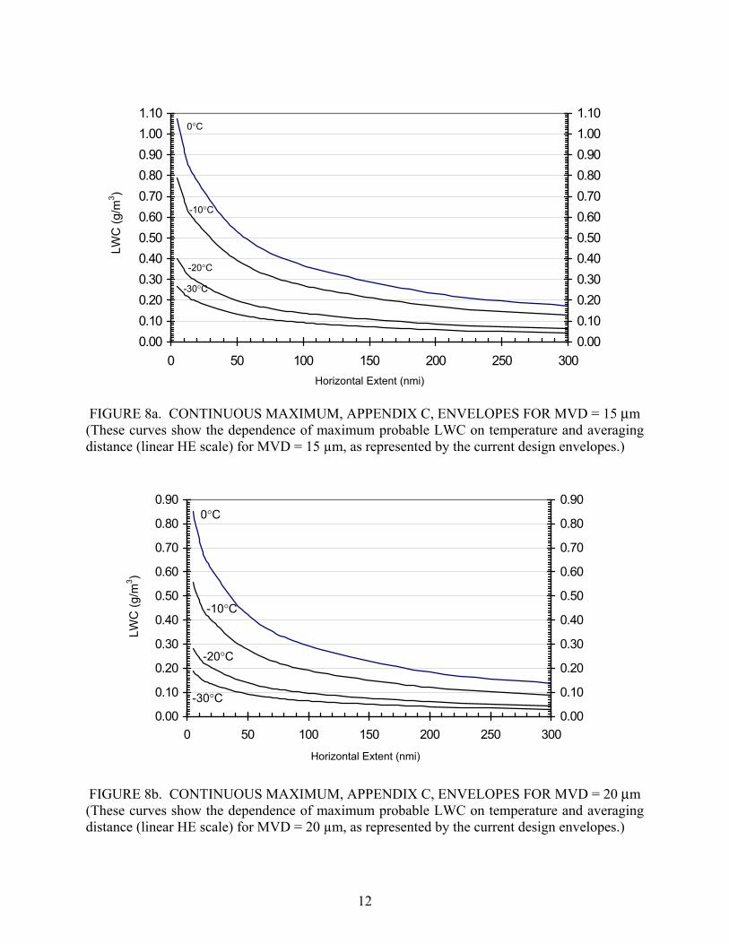
All design points and test points (distance-averaged LWCs) can be plotted on any of these distance-based graphs without having to adjust anything for exposure distance. Each LWC average is simply plotted above its averaging distance on the horizontal axis. An example is shown in figure 12 where about 3500 icing encounters of all distances and types are plotted on the same graph.

LWC

(g/m

3 )


16

0

1

2

3

4

5

6

0.1 1 10 100

O - 1940s NACA Datao - 1950s NACA Datat - Modern U.S. Summer Data+ - Modern U.S. Winter Datax - Modern Foreign Layer Cloudsn - Modern Foreign Convective Clouds

FIGURE 12. THE ENTIRE SUPERCOOLED CLOUD DATABASE (6600 Icing Events Totaling 28,000 nmi in Icing Conditions)

(LWCs Greater than 2 g/m3 are from Convective Clouds) These data points can now be compared directly to the distance-based Appendix C envelopes, no matter what the averaging distances. 2.2.3 Graphing Flight Data.

In natural icing flights, the variables, especially LWC, are usually variable during the overall exposure. A logical and helpful way to view variable data is in graphical form where the variables are plotted against distance (or time) during the exposure. Examples of this are shown in the scatter plots of LWC in figures 13 and 14. Figure 13 shows a sample 10-minute exposure in icing conditions (supercooled clouds). It illustrates a time history of LWC plotted from data entered into a computerized spreadsheet. The plotted points (circles) are 5-second averages from a hot-wire LWC meter or from an electro-optical droplet size spectrometer. Figure 14 shows the same exposure in an equivalent, distance-based graph. At an airspeed of 150 kt, the aircraft traveled 25 nmi during the 10-minute exposure.

LWC

(g/m

3 )


! -1940s NACA Data □ - 1950s NACA Data ♦ - Modern U.S. Summer Data + - Modern U.S. Winter Data × - Modern Foreign Layer Clouds g - Modern Foreign Convective Clouds

17

0.00

0.05

0.10

0.15

0.20

0.25

0.30

0.35

0.40

0 60 120 180 240 300 360 420 480 540 600

Cloud Gap

Cumulative Average LWC

FIGURE 13. TIME PLOT OF SAMPLE FLIGHT DATA (LWC)

0.00

0.05

0.10

0.15

0.20

0.25

0.30

0.35

0.40

0 5 10 15 20 2510

15

20

25

30

35

40

45

50

MVD

(µm

)

Cloud Gap


MVDs

FIGURE 14. DISTANCE PLOT OF SAMPLE FLIGHT DATA (LWC) These time or distance histories give an overall picture of the cloud penetrations and instantly reveal the uniformity or the irregularity of the icing conditions during the exposure. The analyst can see how much time was spent in clouds compared to the time in any clear spaces between clouds. Besides plotting instantaneous values of LWC, one can also plot a cumulative or moving average value. (The spreadsheet charting software does this easily.) Both smooth out the irregularities, but the cumulative average automatically provides the usually desired type of average over any subinterval from the beginningnot just at the end of the exposure.

LWC

(g/m

3 ) LW

C (g

/m3 )

Exposure Time (Seconds)

Exposure Distance (nmi)

18

In this example, the cumulative average LWC has been chosen to apply only to time in cloud. That is, cloud gaps (defined as intervals where LWC < 0.05 g/m3) are not included in the average. When a cloud gap is entered by the aircraft, the cumulative average is held at its pregap value until the next cloud penetration begins. This is the reason for the flat portion of the cumulative average curve during the cloud gap. This particular averaging method has the effect of removing any clear air intervals from consideration in computing an average LWC for the cloudy portions of an icing encounter. This customized averaging process can be accomplished by using the proper formula and �If � statement in the spreadsheet cells in the Cum. Avg. LWC column. With appropriate labeling, multiple ordinate scales can accommodate any and all of the variables of interest. Usually the LWC, MVD, air temperature, and altitude are the primary variables of interest. If there are only spot measurements, they can be plotted as �points� at the time the samples were taken, as for the MVD in this example. The solid circles in figure 14 are values of MVD computed from hypothetical spot measurements (in this example) of the drop size distribution every 5 nautical miles. 2.2.4 Comparing Test Data With the Envelopes.

The value of the cumulative average LWC at the end of the encounter (or for any subinterval of interest) can then be plotted as a point on any of figures 7 to 12 for comparison with the Appendix C envelopes or with other data. When cloud gaps are present, however, their cumulative distance must be subtracted from the overall exposure distance to obtain the correct HE for use with figures 7 to 12. In the present example as shown in figure 13, the cloud gap occupies 2 nmi out of the 25-nmi exposure, so the final average LWC would be plotted at the 23-nmi position on the HE axis. Figures 7 to 11 are also convenient for graphing test data because the entire exposure can be directly compared with the design envelopes. In the distance-based format, all exposures begin at the left side of the page (at time or distance equal to zero) and migrate across the page until the end of the exposure is reached. 2.2.4.1 An Example.

Figures 15a and 15b show the LWC track in figure 14 superimposed on the envelopes in figures 8 and 10, respectively. In this case, the envelope coordinates were simply added to the computerized spreadsheet containing the flight data, so that both could be plotted on the same chart. In addition, the HE scale has been truncated in figures 15a and 15b to match the limited, 25-nmi exposure distance in this example. The 2-nmi cloud gap has been deleted in order to correctly plot only the net, in-cloud horizontal extent when comparing with the Appendix C envelopes. Figure 15a shows that if the flight level temperature during the encounter were -30°C, then the example LWC would be unusually largethe cumulative average running at the maximum to be expected for this temperature according to the design curve for -30°C. If the temperature during the encounter was between 0° and -10°C, then the icing conditions were probably very ordinary and the LWC was well below the maximum values that could be expected for those temperatures and for MVDs near 15 µm.

19

0.00

0.10

0.20

0.30

0.40

0.50

0.60

0.70

0.80

0.90

1.00

1.10

0 5 10 15 20 25


5-sec Avg. LWC

FIGURE 15a. SAMPLE FLIGHT DATA (CLOUD GAPS REMOVED) COMPARED WITH CONTINUOUS MAXIMUM, APPENDIX C

(MVD = 15 µm, Truncated HE Scale)

0.00

0.10

0.20

0.30

0.40

0.50

0.60

0.70

0.80

0.90

1.00

1.10

0 10 20 30 40 50

MVD = 15 µm

20 µm

25 µm

30 µm

35 µm

40 µm

Cum. Avg. LWC

FIGURE 15b. SAMPLE FLIGHT DATA (CLOUD GAPS REMOVED) COMPARED WITH CONTINUOUS MAXIMUM, APPENDIX C, FOR ICING CONDITIONS NEAR 0°C

LWC

(g/m

3 ) LW

C (g

/m3 )



0°C

-10°C

-20°C

-30°C

20

Figure 15b also shows that the cumulative average LWC was as large as could be expected if the MVD were about 37 µm. For an MVD near 15 µm, the LWC was well below the maximum that could be expected for temperatures near 0° to -10°C. Similar comparison envelopes can be drawn for other representative fixed values of temperature or MVD. Similar envelopes for convective (intermittent maximum) clouds can be prepared as well. 2.3 OTHER WAYS TO DOCUMENT TEST DATA AND COMPARE WITH APPENDIX C OF 14 CFR PART 25.

2.3.1 Converting Appendix C of 14 CFR Part 25 to Time-Based Envelopes.

In-flight exposures may be measured in terms of the distance flown in the icing condition or in terms of elapsed time. Icing wind tunnel exposures and computer simulations are typically reported as timed exposures. The basic graphing format presented so far is in terms of distance, but this is easily converted to time in a computerized spreadsheet. For manual conversion, a time scale can be obtained by dividing the distance scale by the airspeed. Thus, at 200 knots, the 200-nmi mark is also the 60-minute mark. The 20-nmi mark is also the 6-minute mark, and so on. This assumes that the flight speed is roughly constant during the cloud penetration. The resulting time-based Appendix C envelopes are used in the same way as the distance-based envelopes. The only new requirement is that the time-based envelopes must be computed and drawn for the same airspeed as for the test data. This convertible abscissa feature allows wind tunnel and computer-simulated exposures to be plotted on the same time-based graphs as the flight tests and the Appendix C envelopes, if the airspeeds are all about the same. 2.3.1.1 Plotting Icing Tunnel Test Points on Time-Based, Appendix C Envelopes.

In icing wind tunnel exposures and computer simulations, the variables are usually constant during the exposure. They could be shown as level lines from the left side of the graph (time = 0) over to the end of the exposure, or they could be represented by a point plotted at the end of the exposure time. The following example illustrates the additional insight that can be obtained by using time-based versions of Appendix C instead of the conventional LWC vs MVD version. Figure 16a shows the conventional way of plotting tunnel test points on the Appendix C envelopes. In this (real) example, a test article was exposed for seven different time intervals to a LWC of 0.45 g/m3 at an MVD of 20 µm and a temperature of -10°C (+14°F). All seven of these exposures, ranging from 3 to 25 minutes, lie at the same spot on the LWC vs MVD envelopes and are therefore indistinguishable from each other on the graph. The location of the test point dot just above the 14°F curve (at the junction of 20 µm MED and 0.45 g/m3 LWC) misleadingly implies that the selected LWC is just slightly above the probable maximum value for its temperature and MVD, no matter what the exposure time. When a time-based version of Appendix C is used (figure 16b), one can readily see all seven of the exposures properly distributed timewise along the LWC = 0.45 g/m3 line. Moreover, the seven test points are now correctly displayed in relation to the 14°F curve. Contrary to the false impression

21

0.00

0.10

0.20

0.30

0.40

0.50

0.60

0.70

0.80

0.90

10 15 20 25 30 35 40 45

Test Points

FIGURE 16a. CONVENTIONAL CONTINUOUS MAXIMUM, APPENDIX C WITH EXAMPLE TEST POINTS

0.00

0.10

0.20

0.30

0.40

0.50

0.60

0.70

0.80

0.90

0 5 10 15 20 25 30

17.4 nmi

(Test Points)

FIGURE 16b. TIME-BASED, CONTINUOUS MAXIMUM, APPENDIX C ENVELOPES

FOR MVD = 20 µm AND AN AIRSPEED OF 174 kt (200 mph)

Test Points at 20um MVD, 0.45 g/m3 LWC, and -10°C Test Point Exposure Time 1 3 min 2 12 min 3 12.5 min 4 14 min 5 15.8 min 6 16.3 min 7 25 min

0°C

-20°C (-4°F)

-30°C (-22°F)

-10°C (+14°F)

-20°C

-30°C

-10°C (+14°F)

0°C (+32°F)

Exposure Time (min) at 174 kt

MED (microns)

LWC

(g/m

3 )

LWC

(g/m

3 )

17.4 nmi

(Test Points)

22

given by the single dot in figure 16a, one sees that the 3-minute exposure is actually less than the probable maximum LWC (the 14°F curve) for that length of time, while the other exposures are increasingly farther above the probable maximum LWC as the exposure time (horizontal extent) increases. As time goes on, the built-in LWC adjustment factor from figure 33 is causing the envelopes to shrink in magnitude corresponding to the longer exposures (horizontal extents). This is not to say that a fixed LWC of 0.45 g/m3 is inadvisably large, but is just to point out that the old LWC vs MVD version of Appendix C in not an accurate way to plot test points nor to put them in proper perspective. The time-based version of Appendix C is much more suitable for displaying tunnel, computer, and spray rig test points and comparing them to the envelopes. 2.3.2 Converting Appendix C of 14 CFR Part 25 to Water Catch Rate (WCR) Envelopes.

In the above example, the emphasis has been on graphing and comparing the LWC. But in some applications, such as in testing thermal anti-icing systems, the rate of water catch is important. That is, for a given amount of LWC, the speed at which the aircraft flies through it and the droplet collection efficiency of the wing is important in determining how much heat is required to keep the leading edges at a required elevated temperature. Both the speed and shape of the wing determine the water catch rate (WCR) (pounds of water per square foot per minute or grams of water per square meter per minute, for example) within the impingement zone along the wingspan. In this case, the duration of a given WCR is important. In test flights, the available WCR should be steady and persist at least long enough for the surface temperature of the wing leading edge to stabilize for a given flight condition. This means that cloud gaps, if long enough to cause the moving average WCR to change significantly, should be regarded as ending the momentary test encounter. That is, long cloud gaps cannot be ignored as in the previous LWC averages. The beginning of the next cloud penetration may have to be regarded as the beginning of a new test interval. Cloud intervals that do not last long enough for wing temperatures to stabilize may not be useful. The required distance may be the conventional 17.4-nmi design distance, or it could be shorter for a thermal system with large capacity. In the previous data sample, the cloud gap causes the encounter to be broken into two separate intervals. The first interval lasts only for about 2 minutes (about 6 nmi) and is probably too short for testing a heated wing. The second interval lasts nearly 15 minutes and may be a successful encounter for these purposes. Therefore, only this second interval would be used for comparing to the Appendix C envelopes. The water catch rate is computed simply from the equation WCR = (TAS)(Etot)(LWC), (1) where TAS is the true airspeed and Etot is the total collection efficiency of the airfoil section for the available cloud droplets. This formula can be used in the spreadsheet cells to automatically convert LWC values to WCR.

23

The units of WCR are g/m2 per second, for TAS in m/sec, and LWC in g/m3. To convert to g/m2 per minute, multiply this WCR by 60. To convert to lb/ft2 per minute, multiply this WCR by 0.00253. To use a specific example, consider a small airplane whose cruise speed is about 150 kt (77 m/sec) and whose outer wing is a NACA 23012 airfoil with a chord length of 1.07 meters (3.5 feet). This is representative of a Beechcraft Queen Air, for example. Droplet impingement codes, such as contained in LEWICE [10] or on the University of Illinois interactive web site [11], can be used to compute the total cloud droplet collection efficiency. For this case one finds Etot is about 0.1 for cloud droplets of about 15 µm diameter. Figure 17 shows, for our example icing encounter, the resulting WCR plotted against distance for the 15-nmi interval after the cloud gap.

0

0.005

0.01

0.015

0.02

0.025

0 5 10 15 20 25

30-sec Moving Average

FIGURE 17. WATER CATCH RATE (WCR) FOR SAMPLE EXPOSURE (CLOUD GAP REMOVED) COMPARED WITH CONTINUOUS MAXIMUM, APPENDIX C,

CONVERTED TO WCR ENVELOPES (for the conditions shown) In order to compare the sample WCR record with the Appendix C envelopes, the latter has to be converted from LWC to WCR curves too. Not only that, but the envelopes have to be reduced by the same collection efficiency factor, Etot, as for the airfoil in the comparison. That is, the envelopes must be regarded as a LWC environment which is penetrated with the same collection efficiency as the actual test conditions.


Wat

er C

atch

Rat

e (lb

/ft2 ) p

er m

in) 0°C

-10°C

-20°C

-30°C

Conditions: MVD = 15 µm Etot = 0.1 TAS = 77 m/s

24

This conversion to WCR envelopes and reduction by Etot is also accomplished by equation 1. One simply inserts the LWC values for each of the envelopes into equation 1 and an equivalent set of WCR envelopes is obtained. These are shown in figure 17. They have the same shape and relative spacing as the previous LWC envelopesthey just have different units and magnitudes. Equation 1 may be thought of as a multiplying factor and a units changer. Figure 17 may be interpreted as follows. If the exposure took place at an air temperature of -30 °C, then the WCR would be about two-thirds of the maximum rate to be expected for that temperature. On the other hand, if the exposure was between 0° and -10 °C, then the available WCR was well below the maximum to be expected for these temperatures. If the thermal ice protection system performed satisfactorily during this 15-nmi exposure, then the entire area under the sample WCR curve could be considered a region of the envelope that was proven safe by this test flight. This is one way to keep score and mark off successfully encountered (or demonstrated safe) regions of the envelopes. 2.3.2.1 Water Exposure Rate (WER).

It is also possible to ignore the collection efficiency and compare what may be called the water exposure rate (WER). In this case, the units are the same as above, but the meaning and magnitudes are different. It is related to the total amount of water in the path of the airfoil, without regard to how much actually accretes as ice. The WER can be used if Etot is unknown, but it must be remembered that the WER does not represent the actual rate of ice accretion. The WERs will be a factor of ten larger than the WCRs for the example airplane described above, but the WER curve will lie in the same position as before, relative to the WER envelopes. That is, the comparison with the envelopes will still be the same. 2.3.3 Converting Appendix C 14 CFR Part 25 to Total Water Catch (TWC) Envelopes.

Another item of interest for an icing encounter may be the total amount of ice accreted on certain components, such as unprotected surfaces. Here, the rate of water (ice) accumulation may not be important, but rather the total water catch during the encounter(s). The TWC may be useful for estimating the weight of ice accreted on aircraft components, except for any losses due to shedding or melting. At least the TWC can be another way to measure test exposures and evaluate their significance. (A question often asked during natural icing flight tests is �What is an adequate icing exposure?�) The TWC can be useful for documenting or rating test exposures. For example, specified values of TWC could serve as target values to be achieved in-flight in order for an exposure to qualify as adequate for the purposes in mind. The TWC is computed simply from the equation TWC = (Etot)(HE)(LWCavg), (2) where HE is the total distance over which LWC is nonzero, and LWCavg is the cumulative average LWC over the cloudy intervals corresponding to HE. Another requirement is that the outside air

25

temperature (OAT) be below 0°C during the encounter. (It may be better to require that the total air temperature (TAT) be below 0°C so that the intercepted water will be known to stick.) Another way to compute TWC is to sum the incremental products of (LWC)(Etot)(AD) over the entire exposure, where AD is the averaging distancethe incremental distance over which LWC is averaged for recording during the test flight. For example, if the LWC is recorded as 5-second averages during flight, then the TWC is given by TWC = Sum{(Etot)(AD)(LWC)}, (3) where each quantity in parentheses is the 5-second value of that variable. If Etot may be regarded as practically constant during the exposure, then the only variable for each 5 seconds is the LWC. Then equation 3 may be written TWC = (Etot)Sum{(AD)(LWC)}, (4) where the LWCs are 5-second averages and AD = (TAS)(5 seconds). This formula (equation 4) in the spreadsheet cells will easily compute the TWC for each 5-second interval, and the resulting column of TWCs can simply be summed. Thus, TWC nicely tallies only the cloudy parts of the encounter4. The units of TWC are g/m2, for AD or HE in meters, and LWC in g/m3. To convert to pounds per square foot, multiply this TWC by 4.23×10-5. Like LWC and WCR, TWC may be plotted against HE and compared to Appendix C envelopes converted to TWC. This conversion to TWC is accomplished by inserting LWC and HE pairs from table 1 into equation 2. The result is shown in figure 18 where the incremental TWC for the example airplane flying in the sample exposure is drawn for comparison. In this case, the TWC envelopes have a different shape than for the LWC and WCR envelopes. Although TWC is insensitive to cloud gaps (in the cloud gap LWC = 0 and there is no contribution to equation 3 or 4), cloud gaps must be removed when plotting incremental TWCs versus distance in comparison with the envelopes. This is because the envelopes assume continuous cloudiness. By including cloud gap distances in the sample TWC, the HE will be falsely extended. In the same way, if only the final value of TWC is plotted as a single test point on the envelopes, the distance traveled in cloud gaps must be subtracted from the total encounter distance. Otherwise, the test point will again be plotted at too large a value for HE.

4 Note that if there are cloud gap distances in the HE it is not correct to shortcut the procedure and sum all the LWCs and then multiply by the total HE for the encounter. The computed TWC would then be too large.

26

0.000.010.020.030.040.050.060.070.080.090.100.110.120.130.140.15

0 5 10 15 20 25

FIGURE 18. TOTAL WATER CATCH (TWC) FOR SAMPLE EXPOSURE (CLOUD GAP REMOVED) COMPARED WITH CONTINUOUS MAXIMUM, APPENDIX C,

CONVERTED TO TWC ENVELOPES (For the conditions shown) Figure 18 may be interpreted as follows. If the exposure took place at an air temperature of -30°C, then, because the TWC data lie on top of the -30°C envelopes curve, the available TWC is the maximum to be expected for stratiform clouds at that temperature. On the other hand, if the exposure was between 0° and -10°C, then, because the TWC data are well below the 0° and -10°C envelope curves, the available TWC is well below the maximum that could be expected for these temperatures. The area under the TWC data curve could also be blacked out as a way of indicating the portion of the TWC envelopes that have been covered by this test flight. 2.3.3.1 Acceptable Exposures.

Another question often asked about natural icing flights is what is an adequate exposure, or how much exposure is enough? A minimum flight exposure could be set in terms of TWC for this purpose. One possibility is to require an accumulation of TWC to match some design point or other reference point on the envelopes. Such a reference point could be the maximum TWC from the envelopes for a 17.4-nmi exposure at the same temperature as the available icing conditions during the test flight. For example, if the flight-test temperature was -10°C, then from the -10°C envelope curve in figure 18 it is seen that a 17.4-nmi exposure would result in a TWC of about 0.08 lb/ft2. This value, then, could be used as the target TWC to be achieved during the test flight. This is an arbitrary way of setting flight-test criteria, but it illustrates one possibility. There may be better reasons for selecting other values, depending on the goals of the flight test. For the example data used in figure 18, a TWC of only 0.033 lb/ft2 was achieved during the 23 nmi of in-cloud exposure. This is about 0.05 lb/ft2 short of the example criterion set above. Because TWC is an additive quantity, the test aircraft can turn around and repenetrate the cloud layer as


Tota

l Wat

er C

atch

(lb/

ft2 )

-10°C

-20°C

-30°C

0°C Conditions: MVD = 15 µmEtot = 0.1 TAS = 77 m/s

27

many times as necessary to build up the TWC to the required amount. If the sample exposure remained at its original LWC values during subsequent penetrations, then about 1.5 more passes would be required to reach a TWC of 0.08 lb/ft2. This means about 58 nmi of total exposure in the cloud, using TWC as the measure of an acceptable exposure. This can be plotted on a continuation of figure 18 if the HE scale is extended to at least 60 nmi. 2.3.3.2 Total Water Exposure (TWE).

As with the water catch, if Etot is unknown, then it may be left out of equations 2 to 4. In this case, these equations no longer give TWC but the TWE instead. TWE is the total amount of water present in the path swept out by the airfoil (or other aircraft component), without regard to how much actually collects on the airfoil and sticks as ice. 2.3.4 Converting Appendix C of 14 CFR Part 25 to Icing Severity (Intensity) Envelopes.

Another way to judge, or at least to document, test exposures is to report whether the encounters correspond to a trace, light, moderate, or severe icing condition. Unfortunately, the definitions of icing intensities in use at this writing [12] are not helpful for this purpose because they make no quantitative connection with LWC or any other measure of the icing atmosphere. The current definitions give no way at all for computing the icing intensities. One remedy has been suggested [13] in which the icing intensities are linked to the rate of ice accretion on a clean, unheated airfoil or other aircraft component. The proposed relationship is as follows:

Icing Intensity Time to Accumulate 1/4 inch of Ice Trace Over 1 hour Light 15 to 60 minutes Moderate 5 to 15 minutes Intense 5 minutes or less

Thus, if 10 minutes are required for 1/4 inch (6 mm) of ice to accumulate on the component of interest, then that corresponds to a moderate icing intensity for that component5. These icing rates (and hence the intensity category) can now be computed because the icing rates can be related in a quantitative way to LWC, the droplet collection efficiency, and the airspeed, primarily. In particular, it can be shown [13] that the icing rate is given by dD/dt = (A)(LWC)(ß)(TAS) (5) where dD/dt is the rate of accretion in inches per minute, ß is the peak collection efficiency6 along the leading edge of the airfoil, and A is a constant with a value near 0.0015.

5 Other components (antennae, stores, weapons, pylons, engine inlets, winglets and other sections of the wing, and even other aircraft) may individually have different icing intensities in the same icing cloud, depending on their geometry and airspeed, and therefore, on their droplet collection efficiency.

6 In this application, ß is used instead of Etot because the ice depth is measured at the location of the fastest buildup, which is where ß, the local collection efficiency is largestinitially along the stagnation line. Etot refers to the bulk ice accretion over the full leading edge of the surface between the droplet impingement limits.

28

0

10

20

30

40

50

60

0 5 10 15 20 25

0.00

0.05

0.10

0.15

0.20

0.25

0.30

0.35

0.40

0 5 10 15 20 25

For our example airfoil (NACA 23012) with a chord of 1.07 m and TAS = 150 kt, the values of A and ß are 0.0011 and 0.45, respectively, for typical cloud droplets of around 15 µm in diameter. The proposed definitions above are actually written in terms of the time required for 1/4 inch of ice to accumulate. This time quantity is obtained by solving equation 5 for dt to get dt = dD/{(A)(LWC)(ß)(TAS)} = 3.37/LWC (6) where dt is in minutes, dD = 1/4 inch, and dD/{(A)(ß)(TAS)} = 3.37. The icing intensity is, thus, simply obtained by dividing the LWC into the appropriate constant (3.37 in this case). Figure 19 shows the result for the sample icing exposure. The upper panel in figure 19 repeats the original LWC record (from figure 13), and the lower panel shows the corresponding icing intensity along the way.

FIGURE 19a. DISTANCE PLOT OF SAMPLE FLIGHT DATA (LWC)

FIGURE 19b. ICING RATE FOR SAMPLE EXPOSURE



LWC

(g/m

3 ) Ti

me

to A

ccum

ulat

e1/4

inch

(m

inut

es)

Intense

Light

Moderate

Cloud Gap


29

The lower panel may be interpreted as follows. For the first 7 minutes, the airfoil (outer wing in this example) was exposed to moderate icing conditions until the cloud gap was reached. Within the gap the icing rate is zero and there is no icing intensity. Upon entering the second portion of the clouds, the LWC is a little less than before, and the time to accumulate 1/4 inch of ice hovers around 20 to 25 minutesa light icing condition, according to the proposed definitions. If the pilot were operating the deicing boots manually each time a quarter inch of ice built up, then the boots would have to be cycled only occasionallyabout once every 20 minutes to half an hour, if the airplane were to continue in icing conditions like the second part of the sample penetration shown here. Note that this intensity rating system can be used for all icing exposuresnatural icing, wet wind tunnels, tanker sprays, and even computer simulations. It can also be used as a measure of the available icing conditions even for heated, anti-iced wings where no ice will actually accrete. In this case, it represents the amount of ice that could build up if the ice protection were turned off, and it is also a way to illustrate the sensitivity of a particular component to ice accretion in general. 2.3.4.1 Converting Appendix C of 14 CFR Part 25 to Icing Intensity Envelopes.

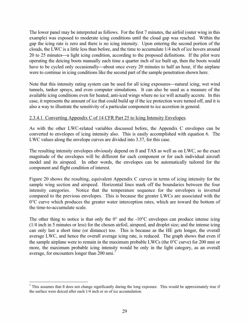
As with the other LWC-related variables discussed before, the Appendix C envelopes can be converted to envelopes of icing intensity also. This is easily accomplished with equation 6. The LWC values along the envelope curves are divided into 3.37, for this case. The resulting intensity envelopes obviously depend on ß and TAS as well as on LWC, so the exact magnitude of the envelopes will be different for each component or for each individual aircraft model and its airspeed. In other words, the envelopes can be automatically tailored for the component and flight condition of interest. Figure 20 shows the resulting, equivalent Appendix C curves in terms of icing intensity for the sample wing section and airspeed. Horizontal lines mark off the boundaries between the four intensity categories. Notice that the temperature sequence for the envelopes is inverted compared to the previous envelopes. This is because the greater LWCs are associated with the 0°C curve which produces the greater water interception rates, which are toward the bottom of the time-to-accumulate scale. The other thing to notice is that only the 0° and the -10°C envelopes can produce intense icing (1/4 inch in 5 minutes or less) for the chosen airfoil, airspeed, and droplet size; and the intense icing can only last a short time (or distance) too. This is because as the HE gets longer, the overall average LWC, and hence the overall average icing rate, is reduced. The graph shows that even if the sample airplane were to remain in the maximum probable LWCs (the 0°C curve) for 200 nmi or more, the maximum probable icing intensity would be only in the light category, as an overall average, for encounters longer than 200 nmi.7

7 This assumes that ß does not change significantly during the long exposure. This would be approximately true if the surface were deiced after each 1/4 inch or so of ice accumulation.

30

FIGURE 20. CONTINUOUS MAXIMUM, APPENDIX C, CONVERTED TO ICING INTENSITY ENVELOPES (for conditions shown)

Another fact to point out is that at an outside temperature of 0°C, no ice may actually form at all, due to the dynamic heating of the wing due to the airspeed. These curves have to be regarded as theoretical maximum icing conditions, and the actual icing rate may be less due to dynamic heating when the total air temperature is near or greater than 0°C. 2.3.4.2 Comparing Icing Intensity With the Envelopes.

Figure 21 shows the sample icing exposure plotted on the icing intensity envelopes. The light irregular curve is a trace of the 5-second icing intensity, while the heavy irregular curve is a smoothed, 30-second moving average of the same. As was seen in the lower panel of figure 19, the sample icing intensity gradually tapers off from moderate to light as the encounter proceeds. The fact that the sample icing intensity trace lies above the -30°C envelope means that the sample icing intensity along the path was not as great as that which would result from maximum probable LWCs at -30°C for this airfoil and the stated conditions. Note that, as in all cases when comparing to the envelopes, all cloud gaps have been removed so that true horizontal extents are being compared. Thus, the observed (or computed) icing intensity for a given component can be plotted on this graph as one way to document the �robustness� of the exposure. It is an informative way of comparing test data to a customized but equivalent version of Appendix C.


Conditions: MVD = 15 µm Airfoil = NACA 23012 Chord = 1.07 m TAS = 150 kt

Min

utes

to A

ccum

ulat

e 1/

4 in

ch

Moderate

Intense

Light

Trace

-30°C

-20°C

-10°C 0°C

0

10

20

30

40

50

60

70

80

0 50 100 150 200 250 300

31

FIGURE 21. SAMPLE ICING INTENSITY (CLOUD GAP REMOVED) COMPARED

WITH CONTINUOUS MAXIMUM, APPENDIX C, CONVERTED TO ICING INTENSITY ENVELOPES (for conditions shown)

2.3.5 Using an Icing Rate Meter to Document Test Exposures.

The foregoing examples all assume that the LWC is known or being measured during the test exposures. Some of the examples also require that the MVD be known or computed from a measured drop size distribution, although this may not be as essential as the LWC measurement.8 Neither LWC nor drop size is easy to measure, reliably. The old way of estimating these variables was to expose rotating cylinders and soot, powder, or oil-coated slides to the airstream during cloud passes. Usually a window replacement or an access hole cut through the fuselage was needed to get these cloud samples. Nowadays, LWC is preferably measured either with a hot-wire probe or by integrating an electronically measured drop size distribution. These can give a continuous, second-by-second record of LWC and drop size during passage through the clouds. Unfortunately, the commercially available hot-wire devices are notoriously prone to drift and other operational and calibration problems which require constant supervision and an experienced operator and data analyst. Drop size measurements are best done with modern, digital, electro-optical probes designed for this purpose. Unfortunately, these are even more complicated and finicky to operate reliablyespecially in icing conditions and/or at airspeeds greater than about 150 kt. In addition, these LWC and drop size probes must be mounted securely at appropriate positions external to the fuselage or under a wing or on the vertical

8 Conventionally, some measurement of MVD has been required during test exposures in order to know whether the MVD was greater than 15 µm, indicating that the test conditions were within the Appendix C envelopes. Often, test results have been arbitrarily disregarded if the MVD were less than 15 µm.

0

10

20

30

40

50

60

70

80

0 5 10 15 20 25 30 35 40 45 50


Min

utes

to A

ccum

ulat

e 1/

4-in

ch

IntenseModerate

Light

Trace

Conditions:MVD=15 µmAirfoil = NACA 23012Chord = 1.07 mTAS = 150 kt

-30 C

-20 C

-10 C0 C

30-sec Moving Average


Min

utes

to A

ccum

ulat

e 1/

4 in

ch

32

stabilizer of the aircraft being tested. Along with running power and data cables to these external probes, this is often expensive, if not impractical, to do on a production aircraft. A better practice may be to use suitable, commercially available icing rate meters that are often normally installed on the aircraft anyway. The Appendix C envelopes can be converted from LWC to icing rates computed specifically for the icing rate meter in use. Measured icing rates can then be used to directly evaluate icing exposures without the need for LWC or drop size measurements. This would greatly simplify the icing flight-test work. No special research equipment is needed and, in addition to dedicated icing test flights, icing encounters of opportunity can be used during flights for other purposes, even in-service flights. This would help build up the database of icing exposures for the particular aircraft model beyond the usually limited, dedicated icing test flights. As an example, consider the Rosemount model 871-FA icing rate meter. The essential feature is the 1/4-inch-diameter sensitive element which projects into the airstream, usually alongside the forward fuselage, below or ahead of the cockpit. As ice builds up on the sensitive rod, a proportional analog output voltage is generated for recording. When an ice thickness of about 0.5 mm is reached, a heater is automatically energized to melt and evaporate the accumulated ice. The output voltage then drops to its baseline (uniced) value, the heating stops, and the ice accumulation can resume as soon as the TAT of the rod cools to below 0°C. An example of the output signal from an actual icing encounter is shown in figure 22a. The sawtooth voltage clearly documents when icing was occurring and the ascending slope during the accumulation intervals is proportional to the ice accumulation rate. For model 871-FA icing detectors set for a nominal 0.5 mm of ice over a 4-volt output range (1-5 v), the ice accretion rate in mm/min is given by

(sec)

)(5.7min

sec60(sec)

)(4

5.0min)/(t

voltsVt

voltsVvolts

mmmmRate∆

∆=×∆

∆×= (7)

where ∆V/∆t is the slope of the output voltage signal. This can be easily computed from the record if the analog output voltage is recorded with sufficient time resolution (e.g., every second) during the encounters. 2.3.5.1 Converting Appendix C of 14 CFR Part 25 to Icing Rate Envelopes.

These measured icing rates can also be compared to Appendix C if figures 1, 4, or 7 are converted from LWC to icing rate on the vertical axis. The rate of ice accretion on the sensitive element is given by equation 5 on a previous page, namely ( )( )( )( )( )4.25min)/( TASLWCAmmRateIcing β= (8)

33

FIGURE 22a. EXAMPLE OF THE ROSEMOUNT MODEL 871-FA ANALOG OUTPUT

VOLTAGE DURING A PASSAGE THROUGH NATURAL ICING CONDITIONS For cloud droplets, β ≅ 0.9 for airspeeds of 150 � 250 kt and A slowly changes from 0.0012 to 0.0011 over the same airspeed range. For a given airspeed, the above equation can be used to convert LWC to icing rate, thereby converting figures 1, 4, or 7 into icing rate envelopes tailored specifically for a 1/4-inch-diameter cylinder. This is shown in figure 22b for the continuous maximum envelopes. Note that the envelopes have the same shape as the original (figure 1) but icing rate has replaced LWC on the ordinate axis.

0.00

0.50

1.00

1.50

2.00

2.50

10 15 20 25 30 35 40 45

Ludlam limit for indicated OAT

Icing rate 9?% limit for indicated OAT and MVD, without Ludlam limit effect

FIGURE 22b. APPENDIX C (CONTINUOUS MAXIMUM) IN TERMS OF ICING RATE ON A 1/4-inch DIAMETER CYLINDER AT 100 kt TAS (using collection efficiency = 0.9 for all drop sizes)

Icing Rate (mm/min) = (0.0012)(LWC)(0.9)(TAS)(25.4)

-20°C

-30°C

-10°C

0°C -15°C

-10°C

-5°C

MVD (microns)

Icin

g R

ate

(mm

/min

) on

1/4-

inch

dia

. Cyl

inde

r

Rosemount Ice Detector (Volts)

34

Figure 22c is the same thing for an airspeed of 150 kt but in the distance-based format.

FIGURE 22c. APPENDIX C (CONTINUOUS MAXIMUM) IN TERMS OF ICING RATE ON A 1/4-inch DIAMETER CYLINDER AT 150 kt TAS IN A DISTANCE-BASED FORMAT

(These curves show the dependence of maximum probable icing rate on temperature and averaging distance for MVD = 15 mm, as represented by the current design envelopes.)

2.3.5.2 Ludlam Limit Effects.

One difference with an ice accretion probe is that, depending on the in-cloud temperature, or more precisely, on the TAT of the probe, the greater LWCs in the upper parts of the envelopes may not be measurable in terms of icing rate. This is due to incomplete freezing of the impinging water if the LWC exceeds a certain value for a given air temperature and airspeed. This limiting value of LWC is known as the Ludlam limit [14]. The Ludlam limit for static air temperatures of -5°, -10°, and -15°C are shown in figures 22b and 22c by the horizontal dashed lines. The -5°C line in figure 22b, for example, means that icing rates greater than 0.6 mm/min (on a 1/4-inch-diameter cylinder at 100 kt) will lag the available LWC due to incomplete freezing. To a first approximation, the Ludlam limit depends mainly on the LWC, OAT, and TAS, and not so much on the size of the accreting object. Thus, the (unheated) airframe components will generally not accrete ice if the ice detector does not. A possible exception9 is runback icing in 9 Another exception is when the probe is installed at an aerodynamically incorrect position on the aircraft. In this case the sensitive element could be either shadowed from certain drop sizes or even exposed to an artificially concentrated flow of cloud droplets, depending on the droplet trajectories in the airstream at the probe location.

Icin

g R

ate

(mm

/min

) on

1/4-

inch

dia

. Cyl

inde

r at 1

50 k

t


35

some cases. That is, when the TAT is near 0°C along the leading edge of a wing, for example, water not freezing there may run back and freeze in a low-pressure area (dynamically lowered temperature zone) farther back on the suction side of the airfoil. A comparison of measured icing rates with the envelopes can be illustrated with the following examples.

Case

Icing Rate (mm/min)


OAT (°C)

A B C D

0.7 0.7 0.5 1.0

10 5 15 8

-6 -6 -3 -5

These are plotted in figure 22c where they should be compared with the upper two curves for 0° and -10°C. The example icing rates fall well below the probable maximum values represented by the solid curves for 0° and -10°C, but those icing rates are not achievable anyway, due to the Ludlam limit effect. As a result, the measured values can be directly compared with the envelopes only below the Ludlam limit lines. Icing rates (case D, for example) can still occur above these lines, but the measured rate will be less than the same LWC would provide in a colder cloud. That is, the icing rate will not increase in proportion to the available LWC when the icing rate exceeds the Ludlam limit for the existing OAT. In general, the icing rate on the 1/4-inch cylinder will be an indication of the icing rate on the leading edge of the airframe surfaces. Although the aircraft may be in a high LWC situation, the icing rate could be low. The icing rate is a useful measurement because it is actually an integrated result of all the variables involved, namely LWC, OAT, TAS, drop size distribution, collection efficiency, and Ludlam limit effects. The icing rate reflects the actual icing situation on the rest of the aircraft regardless of the MVD, and the icing rate is easier to measure than LWC and drop size individually. If drop sizes are not measured, the main drawback seems to be only that it will be unknown whether the icing exposure is within Appendix C, in terms of MVD (see footnote 8). 3. COMPARING TEST DATA WITH NATURAL PROBABILITIES.

3.1 THE DIFFERENCES BETWEEN APPENDIX C OF 14 CFR PART 25 AND NATURE.

The envelopes in Appendix C are design envelopes, which means that they are tailored to show the range of values necessary for consideration in designing ice protection systems for aircraft. They do not show all the values that can exist in nature, nor do they reveal the probability of encountering various LWCs, MVDs, temperatures, or exposure durations in icing conditions. For example, the envelopes do not show any MVDs below 15 µm; whereas in nature one easily finds MVDs down to 10 µm or less. For design purposes, MVDs smaller than 15 µm were not considered to be important, at least for large, thick wingsthe main concern for ice protection engineers in the early

36

1950s. Propellers and helicopter rotor blades are more sensitive to these smaller drop sizes, however. Similarly, only the probable maximum (99th percentile) values of LWC were considered to be appropriate for civil design purposes, so no 95, 90, or 50th percentile values were included. On the other hand, designers of ice protection systems for military aircraft have often voiced a desire for lesser percentile values of LWC where they have the option to accept more risk as a tradeoff against extra weight, space, and electrical power requirements, for example. Despite the limited purpose of the design envelopes, it may be helpful to the aircraft certification office (ACO) or other data evaluators to have some idea of the typical values found in nature, or of the likelihood of encountering different values of LWC and MVD in natural icing conditions. This helps put the submitted data in perspective. This kind of information is available from the large database (28,000 nmi) of measurements in icing conditions, assembled at the Federal Aviation Administration (FAA) William J. Hughes Technical Center [15]. The remainder of this section shows several examples and indicates how they may be used to evaluate and put into perspective, any particular icing condition. 3.2 COMPARING WITH NATURAL LWC PROBABILITIES.

One comparison that is not possible with Appendix C is the question of how common, or uncommon, was a particular test flight icing encounter? Or, how representative of nature is a particular icing wind tunnel exposure or computer simulation? In other words, what is the probability of finding such a test exposure in nature? Figure 23 shows a set of LWC probability curves derived from about 23,000 nmi of flight data in stratiform icing conditions. Any given curve indicates the probability that randomly encountered, stratiform icing conditions will have an average LWC somewhere below the curve. For example, the 50% curve means that half of the LWC averages will lie below the curve and half will lie above it. The 90% curve means that 90% of all LWC averages can be expected to lie below it, for any given averaging distance, or horizontal extent. The sample LWC trace has been plotted on this graph to determine where it lies in the realm of probabilities. It is already known from earlier comparisons to the Appendix C envelopes that the sample encounter contained LWCs considerably below the maximum that could be expected. Figure 23 shows exactly how far below the maximum that is. The encounter seems quite acceptable since the cumulative average LWC is greater than the 50% value the entire time. It starts out at perhaps the 70% level and gradually drifts down toward an average (50%) encounter as the flight proceeds. 3.2.1 Icing Wind Tunnel Tests.

Also drawn on the graph in figure 23 is a horizontal line at LWC = 0.5 g/m3. This represents a steady LWC exposure in an icing wind tunnel. A LWC of 0.5 g/m3 is one of several popular settings for the NASA/Glenn Icing Research Tunnel (IRT) and is near the lowest that can be produced in that tunnel for wind speeds of 100 to 150 kt.

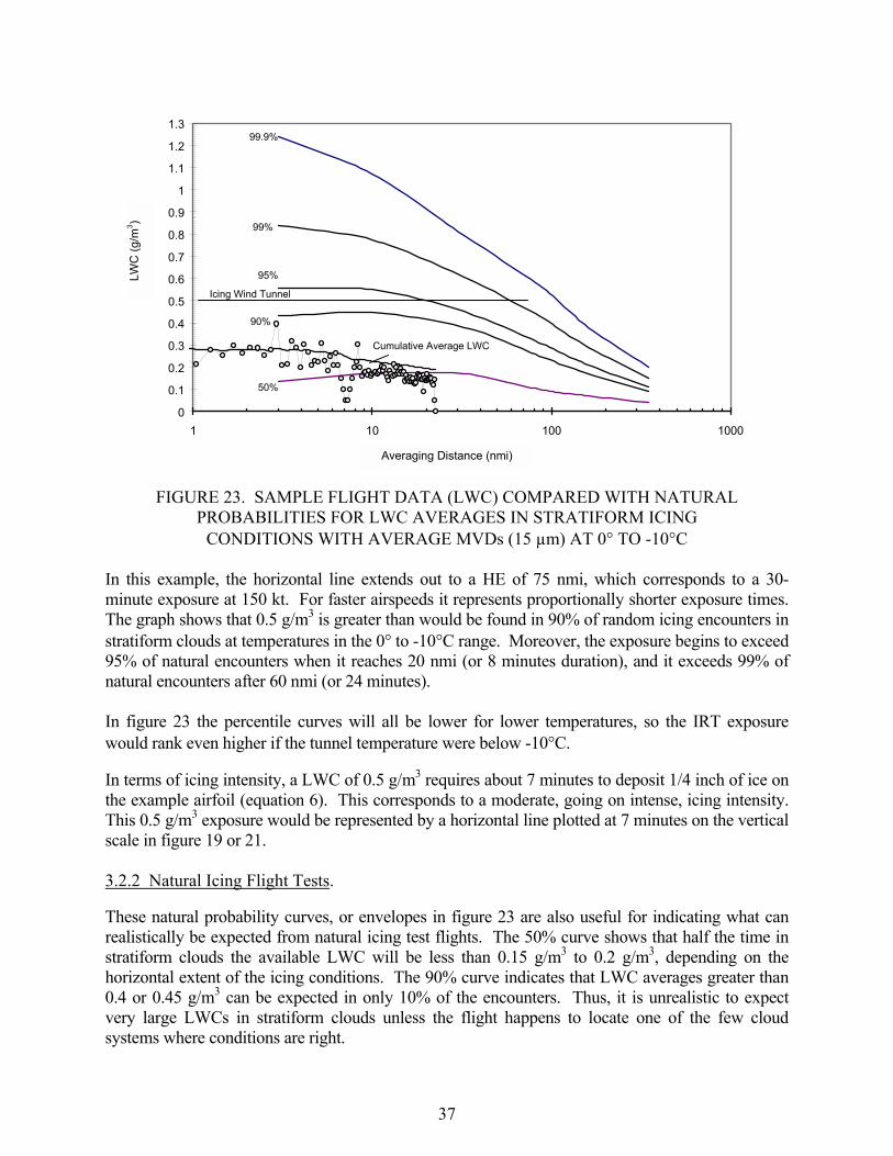
37

0

0.1

0.2

0.3

0.4

0.5

0.6

0.7

0.8

0.9

1

1.1

1.2

1.3

1 10 100 1000

99.9%

99%

95%

90%

50%


Icing Wind Tunnel

FIGURE 23. SAMPLE FLIGHT DATA (LWC) COMPARED WITH NATURAL PROBABILITIES FOR LWC AVERAGES IN STRATIFORM ICING

CONDITIONS WITH AVERAGE MVDs (15 µm) AT 0° TO -10°C In this example, the horizontal line extends out to a HE of 75 nmi, which corresponds to a 30-minute exposure at 150 kt. For faster airspeeds it represents proportionally shorter exposure times. The graph shows that 0.5 g/m3 is greater than would be found in 90% of random icing encounters in stratiform clouds at temperatures in the 0° to -10°C range. Moreover, the exposure begins to exceed 95% of natural encounters when it reaches 20 nmi (or 8 minutes duration), and it exceeds 99% of natural encounters after 60 nmi (or 24 minutes). In figure 23 the percentile curves will all be lower for lower temperatures, so the IRT exposure would rank even higher if the tunnel temperature were below -10°C. In terms of icing intensity, a LWC of 0.5 g/m3 requires about 7 minutes to deposit 1/4 inch of ice on the example airfoil (equation 6). This corresponds to a moderate, going on intense, icing intensity. This 0.5 g/m3 exposure would be represented by a horizontal line plotted at 7 minutes on the vertical scale in figure 19 or 21. 3.2.2 Natural Icing Flight Tests.

These natural probability curves, or envelopes in figure 23 are also useful for indicating what can realistically be expected from natural icing test flights. The 50% curve shows that half the time in stratiform clouds the available LWC will be less than 0.15 g/m3 to 0.2 g/m3, depending on the horizontal extent of the icing conditions. The 90% curve indicates that LWC averages greater than 0.4 or 0.45 g/m3 can be expected in only 10% of the encounters. Thus, it is unrealistic to expect very large LWCs in stratiform clouds unless the flight happens to locate one of the few cloud systems where conditions are right.

Averaging Distance (nmi)

LWC

(g/m

3 )

38

00.10.20.30.40.50.60.70.80.9

11.11.21.31.41.51.6

1 10 100 1000

15,000 ft AGL

10,000 ft AGL

5,000 ft AGL

20,000 ft AGL

2,500 ft AGL

3.3 COMPARING WITH THE NATURAL ALTITUDE DEPENDENCE OF LWC.

The probability curves in figure 23 give the overall likelihood of finding a given LWC average without regard to the actual temperature, MVD, altitude, or season of the year. For example, it is known intuitively that the indicated 99% LWCs cannot realistically be expected at extremely low altitudes near ground level, nor at extremely high altitudes, above 30,000 ft or so, where temperatures are so low that any stratiform clouds are likely to be all ice crystals. There must be some variation in these curves with altitude. Indeed, the 23,000 nmi of stratiform icing cloud data in the database at the FAA William J. Hughes Technical Center can be used to examine the dependence of LWC on other variables such as those mentioned above. Figure 24 shows the 99% LWC limits that are to be expected at several altitude intervals. These limits are based mostly on stratiform clouds, but nonsummer convective clouds with horizontal extents greater than 5 nmi are also included. In this way the user does not have to be concerned whether a particular exposure was in stratiform clouds, wide convective clouds, or a mix of the two. The only thing that matters, realistically, is the likelihood of finding a given LWC average over a given exposure distance in flight, regardless of the type of cloud that is producing it.

FIGURE 24. NATURAL 99% LWC LIMITS VS ALTITUDE (AGL) FOR HIGHEST TEMPERATURES AVAILABLE AT THE ALTITUDE AND

FOR ALL SUPERCOOLED CLOUDS AT 15-20 µm MVD Figure 24 reveals that the upper limit to LWC generally increases with altitude up to about 10,000 ft above ground level (AGL), and then begins to decrease with increasing altitude above that (except for short encounters up to 15,000 ft where convective clouds make a greater contribution to the LWCs). It will also be noted that the 99% LWCs are very similar at 2500 and 20,000 ft, except for short encounters near 20,000 ft where convective clouds again contribute greater LWCs than they do at 2500 ft.


LWC

(g/m

3 )

39

Another, perhaps more helpful way to display the natural altitude dependence of LWC is to draw a range of percentile curves, as was done in figure 23, for each altitude shown in figure 24. Figures 25a to 25e show the results.

0

0.1

0.2

0.3

0.4

0.5

0.6

0.7

0.8

0.9

0 10 20 30 40 50 60 70 80 90

99.9%

99%

95%

90%

50%

FIGURE 25a. NATURAL PROBABILITIES FOR LWC AVERAGES AT ALTITUDES UP TO 2500 ft AGL

0

0.1

0.2

0.3

0.4

0.5

0.6

0.7

0.8

0.9

1

1.1

1.2

1.3

1.4

1 10 100 1000

99.9%

99%

95%

90%

50%

FIGURE 25b. NATURAL PROBABILITIES FOR LWC AVERAGES AT ALTITUDES OF 5000 ft ±2500 ft AGL


LWC

(g/m

3 )

LWC

(g/m

3 )


40

00.10.20.30.40.50.60.70.80.9

11.11.21.31.41.51.61.71.8

0 50 100 150 200 25000.10.20.30.40.50.60.70.80.911.11.21.31.41.51.61.71.8

99.9%

99%

95%

90%

50%

Applies to: All stratiform clouds and nonsummertime convective clouds,flight-level temperatures about 0C to -10C,

and MVD's about 15 µm ± 2.5 µm.(Curves will be lower for temperatures below -10C and for MVD's outside the indicated range)

17.4 nmi

FIGURE 25c. NATURAL PROBABILITIES FOR LWC AVERAGES AT ALTITUDES OF 10,000 ft ±2500 ft AGL

00.10.20.30.40.50.60.70.80.9

11.11.21.31.41.51.61.71.81.9

2

1 10 100 1000

99.9%

99%

95%

90%

50%

FIGURE 25d. NATURAL PROBABILITIES FOR LWC AVERAGES AT ALTITUDES OF 15,000 ft ±2500 ft AGL



LWC

(g/m

3 ) LW

C (g

/m3 )

41

0

0.10.2

0.3

0.40.5

0.60.7

0.8

0.91

1.1

1.21.3

1.4

0 10 20 30 40 50 60 70 80 90 100

99.9%

99%

95%90%

50%

FIGURE 25e. NATURAL PROBABILITIES FOR LWC AVERAGES AT ALTITUDES OF 20,000 ft ±2500 ft AGL

Figure 26 shows our sample icing encounter compared with the LWC percentile curves from figure 25a, assuming that the sample data were actually collected at some altitude below 2500 ft AGL. In this case, the cumulative average LWC lies between the 50% and the 90% envelopes, indicating that this exposure is above average in LWC for this altitude range. This sample exposure would therefore seem to be an acceptable encounter, based on its relatively high ranking among the percentile curves.

0

0.1

0.2

0.3

0.4

0.5

0.6

0.7

0.8

0.9

0 10 20 30 40 50 60 70 80

99.9%

99%

95%

90%

50%Cumulative Average LWC

FIGURE 26. SAMPLE FLIGHT DATA (CLOUD GAP REMOVED) COMPARED WITH NATURAL PROBABLILTIES FOR LWC AVERAGES AT

ALTITUDES UP TO 2500 ft AGL

LWC

(g/m

3 )


LWC

(g/m

3 )


42

3.4 COMPARING WITH THE NATURAL MVD DEPENDENCE.

The natural probability of finding various LWC values also depends on the MVD for the cloud droplet population that is present in the cloud at the time and location of the penetration. The database of supercooled cloud variables reveals that the natural dependence of LWC on MVD is somewhat different than that indicated in the Appendix C design envelopes. Figure 27 shows the natural variation of 99% LWC for several increments in MVD. Several facts stand out. Firstly, the larger the MVD above 15 µm, the rarer that MVD is in nature. The percentages in parentheses after the label for each curve indicate the relative percentage of encounters having larger MVDs. Secondly, the larger the MVD the shorter the distance over which it can exist. The overall average MVD for stratiform clouds is about 15 µm, and this, therefore, represents an equilibrium or preferred condition for cloud droplet populations in these clouds. Deviations away from 15 µm are apparently an unstable state, unsustainable both in time and distance in stratiform clouds. In contrast, the design envelopes (figure 10, for example) make no statement about relative probabilities and they assume that all MVDs can persist over distances of 300 nmi or more.

0

0.1

0.2

0.3

0.4

0.5

0.6

0.7

0.8

0.9

0 10 20 30 40 50 60 70 80 90 100 110 120 130 140 150 160 170 180 190 2000

0.1

0.2

0.3

0.4

0.5

0.6

0.7

0.8

0.915µm (32%)

20µm (12%)

25µm (4%)

30µm (2%)

40µm (0.5%)

17.4 nmi

68% of all MVDs are < 15 µm,77% of all MVDs are = 15 µm ± 5 µm

--------(Percentages by each curve give fraction

of MVDs that have been found largerthan the indicated MVD)

FIGURE 27. NATURAL HE LIMITS AND 99% LWC LIMITS FOR SELECTED, SUSTAINED MVDs IN STRATIFORM CLOUDS AT 0° TO -10°C

(curves will be lower for temperatures below -10°C) Both Appendix C and figure 27 show that the largest available LWCs occur only when the MVD is near 15 µm.

LWC

(g/m

3 )


(Curves will be lower for temperatures below �10°C)

43

Figure 28 shows our sample icing encounter compared with the 99% LWC curves from figure 27. In this case, the position of the cumulative average LWC curve above the 40 µm MVD envelope clearly rules out the possibility that the encounter-wide average MVD was as large as 40 µm. It is even unlikely that the MVD could have been 30 µm, because the encounter lasted as long or longer than the maximum 20 nmi or so that any 30 µm MVD condition is expected to last. More than likely the MVD for the sample encounter was near 15 µm ±5 µm, in which case the sample LWC is about 30% of the maximum LWC that could be expected.

0

0.1

0.2

0.3

0.4

0.5

0.6

0.7

0.8

0.9

1 10 100

15µm (32%)

20µm (12%)

25µm (4%)

30µm (2%)

40µm (0.5%)

17.4 nmi68% of all MVDs are < 15 µm,77% of all MVDs are = 15 µm ± 5 µm.


FIGURE 28. SAMPLE FLIGHT DATA (CLOUD GAP REMOVED) COMPARED WITH NATURAL 99% LWC LIMITS FOR DIFFERENT MVDs

3.5 COMPARING WITH NATURAL HORIZONTAL EXTENTS.

The following table gives some statistics on the durations of nearly 2000 icing encounters recorded during intentional searches for icing conditions on research flights. In table 4, encounters have been defined as stretches of continuous stratiform cloudiness where any gaps or breaks in the cloud(s) are less than 1 nmi in length. Note that nearly 30% of all encounters last only 2 nmi or less before a break in cloudiness lasting 1 nmi or more is reached. The table also shows that about 90% of all encounters (in layer clouds) are less than 20 nmi long. Therefore, the example exposure of 23 nmi is longer than about 90% of the encounters intercepted by research flights along straight-line flight paths. Icing exposures in actual operations may last longer, cumulatively, if an exposure is counted as the full duration of icing conditions (e.g., a string of continuous cloud intervals) until the aircraft finally exits the icing conditions for good.


LWC

(g/m

3 )

44

TABLE 4. DURATIONS OF ICING ENCOUNTERS (From research flights in layer clouds)

Encounter Duration (nmi)

No. of Cases

Percent of Cases

Cumulative Percent

1 - 2 562 28.1 28.1 3 - 4 323 16.2 44.3 5 - 6 205 10.3 54.6 7 - 8 168 8.4 63.0 9 - 10 134 6.7 69.7 11 - 15 207 10.3 80.0 16 - 20 165 8.3 88.3 21 - 50 192 9.6 97.9 51 - 100 33 1.7 99.6 101 - 350 8 0.4 100.0

1997 3.6 CONVERTING NATURAL LWC PROBABILITIES TO OTHER VARIABLES.

The natural probability curves in figures 23 to 28 can be converted to WCR, TWC, icing severity (intensity), or icing rate in the same way these conversions were done for the Appendix C envelopes in figures 17 to 22. These converted displays may be helpful when these other variables are being measured or are of interest as part of the analyses, review, documentation, and evaluation of the icing encounters by the test team or by the ACO. An example is given in section 3.6.1 where the LWC axis is converted to icing rate. Measurements obtained with an icing rate meter can be compared to natural probabilities of finding icing rates by converting the LWC scale to an icing rate scale in any of figures 23 to 28. As before, this is accomplished with the help of equation 8. Figure 29, converted from figure 23, is one example. Figure 29 is for the particular case of a 1/4-inch cylinder at an airspeed of 150 kt. The four example icing rates used previously on figure 22c are again plotted here using the symbols A, B, C, and D. A linear HE scale is used in figure 29 instead of the logarithmic scale in figure 23. Rates A and B are average for the distances over which they were recorded, while rate D is greater and rate C is lower than average. The 1 mm/min icing rate (D) is above the Ludlam limit for its temperature (-5°C), so the rate may be somewhat less than otherwise possible for the same LWC environment in a colder cloud. If the cloud were warmer or the airspeed faster, all of the icing rates would approach zero if the TAT approached 0°C.

45

0.0

0.5

1.0

1.5

2.0

2.5

3.0

3.5

0 50 100 150 200 250 300 350

50%

90%

95%

99% 99.9%

-5C

-10C

-15C

Ludlam limit for indicated OAT

D

BA

C

FIGURE 29. NATURAL PROBABILITIES FOR ICING RATES ON A 1/4-inch CYLINDER AT 150 kt IN STRATIFORM ICING CONDITIONS WITH AVERAGE MVDs (15 µm) AND

IN-CLOUD TEMPERATURES OF 0° TO -10°C 4. SUMMARY.

This report shows how to convert the conventional LWC vs MED design envelopes in Appendix C of 14 CFR Part 25 and 14 CFR Part 29 to equivalent, but more useful envelopes based on a LWC vs HE format. A number of potential uses are illustrated for the new format, particularly for comparing icing test exposures to the Appendix C envelopes and to natural probabilities of occurrence. The LWC vs HE envelopes can also be recast into envelopes for any other LWC-related variable, such as icing rate or water catch rate, total water catch, and icing intensity, for example. In addition to the Appendix C design envelopes and their derivatives, envelopes are also presented which depict naturally occurring probabilities (99.9%, 99%, 95%, 90%, and 50%) of LWC and the dependence of these probabilities on MVD, temperature, altitude, and even on the season of the year. These can all serve for comparing icing test exposures from natural icing flights, icing wind tunnels, airborne spray tankers, and computer simulations to the design envelopes of Appendix C and to real world statistics for naturally occurring icing conditions. The methods illustrated here provide the icing practitioner with straightforward, understandable, and meaningful ways to document, compare, and evaluate data on icing conditions. They offer a set of working standards for achieving consistency and uniformity among users. Some methods may be

Legend Symbol

Icing Rate

(mm/min)

HE (nmi)

OAT (deg C)

A 0.7 10 -6

B 0.7 5 -6

C 0.5 15 -3

D 1.0 8 -5


Icin

g R

ate

(mm

/min

) Icing Rate (mm/min) = (0.0012)(LWC)(0.9)(TAS)(25.4)

46

more useful than others, depending on the application, but a variety are offered, with examples, to illustrate the possibilities. The example graphs also illustrate the use of computerized spreadsheet software for graphing icing variables and for conveniently adjusting or converting the Appendix C envelopes to fit particular applications. This adds new, modern versatility to the envelopes that are not possible with the conventional printed (fixed) version. These proposed methods are based on extensive work in the Flight Safety Research Section (AAR-421) at the FAA William J. Hughes Technical Center. 5. REFERENCES.

1. Code of Federal Regulations, Title 14 (revised and re-issued annually), Federal Aviation Administration, Washington, D.C. 20591.

2. �Recommended Values of Meteorological Factors to be Considered in the Design of

Aircraft Ice-Prevention Equipment,� NACA Technical Note 1855 (1949), NASA/Ames Research Center, Moffett Field, California 94035.

3. �A Probability Analysis of the Meteorological Factors Conducive to Aircraft Icing in the

United States,� NACA Technical Note 2738 (1952), NASA/Lewis Research Center, Cleveland, OH 44135.

4. �Aircraft Ice Protection,� Advisory Circular 20-73 (1971), Federal Aviation Administration,

Washington, D.C. 20591. 5. �Certification of Part 23 Airplanes for Flight in Icing Conditions,� Advisory Circular

23.1419-2A (1998), Federal Aviation Administration, Washington, D.C. 20591. 6. �Certification of Transport Category Airplanes for Flight in Icing Conditions,� Advisory

Circular 25.1419 (1999), Federal Aviation Administration, Washington, D.C. 20591. 7. �Certification of Transport Category Rotorcraft,� Advisory Circular 29-2A (1987), Federal

Aviation Administration, Washington, D.C. 20591. 8. �Engineering Summary of Airframe Icing Technical Data,� D.T. Bowden et al., Technical

Report ADA-4 (1963), Federal Aviation Administration, Washington, D.C. 20591. 9. �Aircraft Icing Handbook,� FAA Technical Report DOT/FAA/CT-88/8-1 (1991), (3 Vols.),

FAA Technical Center, Atlantic City, New Jersey 08405. 10. �Users Manual for the Improved NASA Lewis Ice Accretion Code LEWICE 1.6,� Wm. B.

Wright, NASA Contractor Report 198355 (1995), NASA/Lewis Research Center, Cleveland, Ohio 44135.

47/48

11. University of Illinois Aircraft Icing Research Group, Website URL (as of June 1999): http://www2.aae.uiuc.edu/icing/main.html.

12. �Aeronautical Information Manual,� Section 7-1-19: �PIREPS Relating to Airframe Icing.� 13. �A Workable, Aircraft-Specific Icing Severity Scheme,� R. Jeck, Paper No. AIAA-98-0094,

AIAA 36th Aerospace Sciences Meeting, January 12-15, 1998. Reprints available from American Institute of Aeronautics and Astronautics, Reston, Virginia 20191-4344.

14. �The Heat Economy of a Rimed Cylinder,� F.H. Ludlam, Quart. J. Royal Meteorological

Society, Vol. 77, No 334 (1951). 15. �A New Database of Supercooled Cloud Variables for Altitudes up to 10,000 Feet AGL and

the Implications for Low Altitude Aircraft Icing,� Richard K. Jeck, FAA Technical Report No. DOT/FAA/CT-83/21 (1983), FAA Technical Center, Atlantic City, New Jersey 08405.

Icing Design Envelopes (14 CFR Parts 25 and 29, Appendix C ...

Documents

Transcript of Icing Design Envelopes (14 CFR Parts 25 and 29, Appendix C ...