BIOINFORMATICS Vol. 21 Suppl. 2 2005, pages ii130–ii136doi:10.1093/bioinformatics/bti1122

Microarrays

A fully Bayesian model to cluster gene-expression profilesC. Vogl1,∗,†, F. Sanchez-Cabo2,†, G. Stocker2, S. Hubbard3, O. Wolkenhauer4

and Z. Trajanoski21Institute of Animal Breeding and Genetics, Veterinärmedizinische Universität Wien, 1210 Vienna, Austria,2Institute for Genomics and Bioinformatics and Christian Doppler Laboratory for Genomics and Bioinformatics,Graz University of Technology, Petersgasse 14, 8010 Graz, Austria, 3Faculty of Life Sciences,University of Manchester, M60 1QD Manchester, UK and 4Institute of Informatics, University of Rostock,18051 Rostock, Germany

ABSTRACTMotivation: With cDNA or oligonucleotide chips, gene-expressionlevels of essentially all genes in a genome can be simultaneously mon-itored over a time-course or under different experimental conditions.After proper normalization of the data, genes are often classified intoco-expressed classes (clusters) to identify subgroups of genes thatshare common regulatory elements, a common function or a com-mon cellular origin. With most methods, e.g. k -means, the numberof clusters needs to be specified in advance; results depend stronglyon this choice. Even with likelihood-based methods, estimation of thisnumber is difficult. Furthermore, missing values often cause problemsand lead to the loss of data.Results: We propose a fully probabilistic Bayesian model to clustergene-expression profiles. The number of classes does not need to bespecified in advance; instead it is adjusted dynamically using a Revers-ible Jump Markov Chain Monte Carlo sampler. Imputation of missingvalues is integrated into the model. With simulations, we determinedthe speed of convergence of the sampler as well as the accuracy ofthe inferred variables. Results were compared with the widely used k -means algorithm. With our method, biologically related co-expressedgenes could be identified in a yeast transcriptome dataset, even whensome values were missing.Availability: The code is available at http://genome.tugraz.at/BayesianClustering/Contact: claus.vogl@vu-wien.ac.atSupplementary information: The supplementary material is avail-able at http://genome.tugraz.at/BayesianClustering/

1 INTRODUCTIONGene-expression levels of essentially all genes can be monitoredwith cDNA or oligonucleotide chips over a time-course or underdifferent experimental conditions. After appropriate filtering and nor-malization, a gene-expression matrix (GEM) is produced. Althoughthe number of genes that can be monitored is generally impressive,the proportion of genes with missing values can be up to 50% in atwo-color microarray experiment.

∗To whom correspondence should be addressed.†The authors wish it to be known that, in their opinion, the first two authorsshould be regarded as joint First Authors.

Clustering methods are widely applied to the GEM in order toidentify subgroups of genes that share properties, e.g. commonregulatory factors, a common function or a common cellular ori-gin. Most of the traditional clustering algorithms are heuristic, e.g.k-means (Tavazoie et al., 1999), hierarchical clustering (Eisen et al.,1998) or self-organizing maps (SOM) (Tamayo et al., 1999). Forsome of these methods, the analyst needs to choose the number ofclusters in advance. This choice affects clustering and is often aquestion that the microarray experiment is expected to address. Fur-thermore, these methods often have difficulties with missing values.Finally, most of the traditional clustering algorithms are determin-istic, assigning a gene unequivocally to a particular cluster accordingto their similarity to other genes. A gene, however, might actually begrouped into several different clusters for biological reasons (Segalet al., 2003).

In contrast to these ad hoc methods, clustering algorithms basedon a probabilistic model provide a consistent framework (Yeunget al., 2001a; Medvedovic and Sivaganesan, 2002; Dougherty andBrun, 2004). In particular, Gaussian mixture models have beenwidely applied to cluster gene-expression data owing to the roughlyGaussian distribution that these data present after appropriate trans-formations (Yeung et al., 2001a; Huber et al., 2002). Frequentistand Bayesian methods can then be used to infer the model paramet-ers. Missing data pose no problem to both methods; with a Bayesianapproach, it is even possible to estimate the distribution of the missingvalues. But inference of the number of clusters remains problematic:with frequentist methods, multiple log-maximum-likelihood valuesneed to be compared, penalizing for increasing model complex-ity (e.g. the Bayesian Information Criterion, BIC, Schwarz, 1978).Alternatively, N -fold cross-validation or variants thereof can beemployed (Yeung et al., 2001b). With a Bayesian approach, thenumber of clusters can be treated as a random variable and theposterior probabilities of different numbers of clusters can be eval-uated. Unfortunately, the only implementation of such an approachapplied to expression data up to date (Medvedovic and Sivaganesan,2002) requires integration of the posterior distribution, which makeshandling of missing values problematic.

In this paper, a fully probabilistic model is proposed and applied tocluster gene-expression profiles from microarray experiments. Thesampling scheme is based on the Reversible Jump Markov ChainMonte Carlo (RJMCMC) (Green, 1995) applied to mixture mod-els (Richardson and Green, 1997) to allow the number of clusters to

ii130 © The Author 2005. Published by Oxford University Press. All rights reserved. For Permissions, please email: journals.permissions@oxfordjournals.org

Bayesian clustering of microarray data

vary. This approach is fully Bayesian since all parameters of interest,including the missing values and the number of clusters, are treatedas random variables and their posterior distribution is approximatedwith RJMCMC. The method forms clusters without the need ofchoosing the number of clusters in advance. It can also deal withreplicate experiments. The model was first applied to simulated data,for which the true clusters were found with a high specificity andsensitivity. Our model also outperformed k-means clustering. Whenapplied to experimental data on the yeast cell cycle (Spellman et al.,1998), the inferred clusters of genes were biologically sensible.

2 MATERIALS AND METHODS

2.1 Probabilistic modelTypically, a microarray dataset consists of the expression levels of N genesmeasured at T different biological conditions. In particular, the T biologicalconditions can be time points. Let i, 1 ≤ i ≤ N index the genes and t ,1 ≤ t ≤ T the time points; furthermore, let the variable xit indicate thepresence of a reliable expression level for the i-th gene at the t-th time point.Generalization to several replicates is straightforward but complicates nota-tion. The algorithm accounts for both missing data as well as replicates. Weaim to characterize the K stochastic processes (indexed by k, 1 ≤ k ≤ K)that generated the N gene profiles �yi = (yi1, . . . , yiT) with 1 ≤ i ≤ N .Missing data are allowed.

The goal of a Bayesian analysis is to determine the marginal posteriorprobability distribution for all parameters of interest. Since for complicatedmodels this distribution cannot be obtained analytically, we will make use ofa Markov Chain Monte Carlo (MCMC) simulation scheme (in particular, anRJMCMC to allow the jump between spaces of different dimensions). Forreasons of speed, the algorithm is implemented in the C++ programminglanguage.

2.1.1 General probabilistic model Let us suppose that K stochasticprocesses generated the N gene-expression profiles observed. We introducethe characteristic matrix ZN×K such that each row vector �zi = {zi1, . . . , ziK}of Z has an entry of one for the cluster into which the i-th gene is currentlyclassified and 0s for all other classes. Let ωk be the weight of class k, with∑

k ωk = 1. One might think of ωk as the probability of the i-th gene to fallinto the k-th cluster before knowing its expression data, i.e. ωk = Pr(zik = 1)

for k = 1, . . . , K .We assume that the number of clusters K is unknown. Following earlier

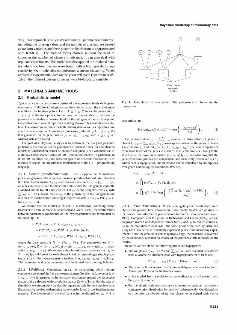
treatment of a similar model (Richardson and Green, 1997), the relationshipsbetween parameters conditional on the hyperparameters are formulated asfollows (Fig. 1):

Pr(Y, Z, �µ, �σ , �ω, K | λ, α, �µ0, κ0, ν0, τ0)

= Pr(Y | Z, �µ, �σ) Pr(Z | K , �ω) Pr( �ω | α, K)

× Pr( �µ | �σ , K , �µ0, κ0) Pr(�σ | K , ν0, τ0) Pr(K | λ) ,

where the data matrix is Y = (�y1, . . . , �yN ). The parameters are �ω =(ω1, . . . , ωK), Z = (�z1, . . . , �zN ), �µ = ( �µ1, . . . , �µK), �µ0 = ( �µ01, . . . , �µ0K)

and �σ = (σ1, . . . , σK). We assume a simple variance–covariance matrix, i.e.�k = σ 2

k IT ×T different for each cluster k and correspondingly simple priors(ν0, τ 2

0 ) for it. The hyperparameters are then, λ, α, �µ0, κ0, ν0, 0 = τ 20 IT ×T .

The parameters and hyperparameters will be defined more thoroughly below.

2.1.2 Likelihood Conditional on zik, i.e. on knowing which mixturecomponent generated the i-th gene expression profile, the i-th data vector �yi ={yi1, . . . , yiT} is assumed to be normally distributed around the respectivemeans of the k-th class with covariance matrix �k = σ 2

k IT ×T . For the sake ofsimplicity, we present here the detailed equations only for the complete data.Equations for the data with missing values can be found in the Supplementarymaterial. The likelihood of the it-th data point conditional on zik = 1 is

Data: Gene

expression

profiles

z

K

w

0 0 0 0

Fig. 1. Hierarchical mixture model. The parameters in circles are thehyperpriors.

proportional to

Pr(yit|µkt, σ2k ) ∝ (σ 2

k )−1/2 exp

(− (yit − µkt)

2

2σ 2k

). (1)

Let us now define nk = ∑Ni=1 zik (number of observations of genes in

cluster k), ykt = (∑

i zikyit)/nk (mean expression level of the genes in clusterk at condition t), and SSQk = ∑

i

∑t zik(yit − ykt)

2 (the sum of squares ofexpression levels of the genes in cluster k at all conditions t). Owing to thestructure of the covariance matrix (�k = σ 2

k IT ×T ) and assuming that thegene-expression profiles are independent and identically distributed (i.i.d.)within each subpopulation, the likelihood can be calculated by multiplyingover genes and biological conditions. Whence,

Pr(�y1, . . . , �yN | Z, �µ, ��)

∝K∏

Pr(�y1, . . . , �yN | Z, �µk , σk)

∝K∏

(σ 2k )−T nk/2 exp

(−

∑Tt nk(ykt − µkt)

2 + SSQk

2σ 2k

). (2)

2.1.3 Prior distributions Proper conjugate prior distributions werechosen that provide little information. Since empty clusters are possible inthe model, non-informative priors cannot be used (Richardson and Green,1997). Compared with the priors in Richardson and Green (1997), we useconjugate instead of independent priors for �µk and σk to reduce complex-ity in the multidimensional case. The same priors were used by Baldi andLong (2001) to detect differentially expressed genes from microarray exper-iments. Since the amount of data is typically large, the posterior is governedby the likelihood, such that the choice of the priors has little influence on theresults.

In particular, we chose the following priors and hyperpriors:

• The weights (0 ≤ ωk ≤ 1 ∀ k and∑

k ωk = 1) are assumed to be drawnfrom a symmetric Dirichlet prior with hyperparameter α set to one.

Pr(ω1, . . . , ωK | K , α) ∼ Dir(α, . . . , α) . (3)

• The prior for K is a Poisson distribution with hyperparameter λ set to 10.A truncated Poisson could also be chosen.

• �zi is sampled from a multinomial generalization of a Bernoulli withPr(zik = 1) = ωk ∀k.

• For the simple variance–covariance structure we assume, we chose aconjugate prior distribution for each σ 2

k independently. Conditional onσ 2

k , the prior distribution of �µk was chosen to be normal with a prior

ii131

C.Vogl et al.

mean of �µ0k and a covariance matrix of �k/κ0 with �k = σ 2k IT ×T

(Gelman et al., 1995):

Pr(σ 2k ) ∼ Inv-χ2(ν0, τ0)

Pr( �µk | �k) ∼ N( �µ0, �k/κ0) .

More complicated models that incorporate dependencies among the differenttime points (Ramoni et al., 2002) could also be used. The variance–covariancematrix we propose corresponds to the unequal volume model by Yeung et al.(2001a). Specifically, we set the prior value of the hyperparameters to κ0 = 1,ν0 = 2 and τ0 = 1. If the data have been properly normalized, we can assume�µ0k = 0 ∀k. The joint prior distribution of �µk and σ 2

k is then

Pr( �µk , σ 2k ) ∝(σ 2

k )−(ν0/2+1) exp

(− ν0τ

20

2σ 2k

)

×∏t

((σ 2

k )−1/2 exp

(− κ0µ

2kt

2σ 2k

)). (4)

2.1.4 Conditional posterior distributions For each gene i independ-ently, the conditional posterior distribution of the vector �zi = {zi1, . . . , ziK }is the multinomial generalization of the Bernoulli distribution:

Pr(�zi | �yi , K , �ω, µ, �) ∝∏k

(Pr(�yi | µk , σ 2k ) · ωk)

zik . (5)

The conditional posterior distribution of the vector of weights is Dirichlet:

Pr(ω1, . . . , ωK | Z) ∼ Dir(α + n1, . . . , α + nK) , (6)

where nk = ∑Ni=1 zik , i.e. the number of genes in the k-th cluster.

The conditional posterior distribution of the means and the variance of thek-th cluster is

Pr( �µk , σ 2k | Y, µ0, κ0, ν0, τ0) ∝ Pr(Y | �µk , σ 2

k )p( �µk , σ 2k )

∝ (σ 2k )−((ν0+T nk)/2+1)

× exp

(− ν0τ

20 + SSQk + (κ0nk/κ0 + nk)

∑t y2

kt

2σ 2k

)

×∏t

((σ 2

k )−1/2 exp

(− (κ0 + nk)(µnkt − µkt)

2

2σ 2k

)), (7)

where µnkt = nkykt/(nk + κ0). Samples from the conditional joint pos-terior distribution of the means and variances can then be obtained asfollows (Gelman et al., 1995): draw σ 2

k from a scaled Inv-χ2(νnk, σ 2

nk), with

νnk= ν0 + T nk and νnk

· σ 2nk

= ν0τ20 + SSQk + (κ0nk/(κ0 + nk))

∑t y2

kt;

draw µkt ∀ t from a normal distribution N(µnkt ,σ 2k

nk+κ0).

2.1.5 RJMCMC sampling scheme The RJMCMC method proceedsby iterating through rounds of cyclically updating the variables in turn:

(1) updating the characteristic matrix Z;

(2) updating the weights ω;

(3) updating the class means and variances ( �µk , σk);

(4) adding or deleting an empty class.

For the first three moves, we use a Gibbs kernel, i.e. we sample from therespective conditional distributions. For the fourth move, we assume thenumber of classes to be drawn from a Poisson prior with mean λ. We suggestan additional class with probability p(K+1) and removal of a random classwith probability pK . For an addition, we create the new class (K + 1) asfollows: we sample a new class variance and a new vector of class means�µK+1 from the prior; we sample φ from a beta(φ | α, Kα + N ), and set thenew class weight of the (K + 1)-th class to ω(K+1)∗ = φ and that of theother K classes to ωk∗ = (1 − φ) · ωk . Note that this choice of the proposaldistribution simplifies the formulas compared with Richardson and Green

(1997). The added class is always empty, such that the likelihood ratio isunity. We then accept the additional class with probability min{1, A}, where

A = Pr(ω∗1 · · · ω∗

K+1 | Z)

Pr(ω1 · · · ωK | Z)· Pr(K + 1)

Pr(K)· 1

beta(φ | α, Kα + N)· J

= (ω1(1 − φ))α+n1−1 · · · (ωK(1 − φ))α+nK−1φα−1

ωα+n1−11 · · · ωα+nK−1

K

× Pr(K + 1)

Pr(K)· 1

φα−1(1 − φ)Kα+N−1· (1 − φ)K−1

= λ

K + 1. (8)

For a deletion, we propose to randomly remove a class without genes. Theacceptance probability for the delete move is min{1, A−1}.2.1.6 Imputation of missing values The missing expression valuescan be imputed with the MCMC method at each step in the iteration bysampling from their conditional distribution given the class, say k,

Pr(yit | . . . ) ∼ N(µkt, σ2k ) .

These imputed values can be treated as data. Over the course of the iteration,an approximation to the posterior distribution of the missing yit can thus beobtained.

2.1.7 Interpretation of the posterior distributions Since jumpingbetween spaces of different dimensions is allowed using the RJMCMCsampling scheme, it is difficult to follow the evolution of each cluster over theiterations. Hence, for each pair of genes, a similarity index was calculated asthe number of iterations that appeared in the same cluster divided by the totalnumber of iterations. The empirical distribution of all the pairwise similarityindexes will be used to determine a threshold; we chose the 95 percentileof the distribution. If the similarity index between two genes is higher thanthis limit, the genes are considered similarly expressed. In other words, acertain gene can be used as a ‘seed’ to generate a cluster of genes with similarprofiles. Figure 2 shows the process in practice.

2.1.8 Implementation details The RJMCMC methods were imple-mented in C++. The post-Bayesian methods were implemented either inR (Ihaka and Gentleman, 1996) or, if performance was an issue, in C++.Code is available in the Supplementary material.

Parallel execution in a Beowulf linux cluster with 50 Intel Xeon 2.60 GHzCPUs considerably reduced the computational time. 10 000 iterations of theRJMCMC were performed; an initial ‘burn-in’ phase of 1000 iterations wasdiscarded. See following section for a justification of the choice of theseparameters.

3 RESULTS FOR THE SIMULATED DATATen data sets simulating a typical microarray experiment with 6000gene-expression profiles (N = 6000) measured across 10 differentconditions (T = 10) were generated. The true number of clusterswas 40. For each simulated dataset a user-specified proportion ofdata was substituted by missing values (10% in the datasets used inthis paper). This way the performance of the method could be testedon datasets with missing values.

3.1 Convergence assessmentIn order to guarantee the convergence and independence of the ini-tial conditions when using iterative simulation, Gelman et al. (1995)suggest running several independent sequences with overdispersedstarting conditions and monitoring the evolution of different inde-pendent parameters. The sequences will have reached convergenceif the within-run variance roughly equals between-runs variation.

ii132

Bayesian clustering of microarray data

Fig. 2. RJMCMC-based clustering of gene-expression profiles: At each iter-ation, the different variables in the model are stored; using the indicatorvariable that assigns genes to the clusters, a matrix of similarity indices isbuilt; given an important gene, others similar to it are found (threshold: the95% percentile of the distribution).

They suggest to estimate the potential scale reduction as

R =√

var + (θ | y)

W, (9)

where var + (θ | y) = (n − 1/n)W + (1/n)B, W is the within-runvariance and B is the between-runs variance, and n is the length ofthe run. Gelman et al. (1995) recommend increasing the number ofiterations if R is much bigger than 1.

When, for the same dataset, the starting number of clustersfor 10 runs was varied between 10 and 100, rapid convergencewas observed (Table 1). Hence, a burn-in period of 1000 itera-tions followed by 10 000 iterations seems sufficient for approximateconvergence (Fig. 3).

3.2 Sensitivity and specificityFor the simulated data, one gene from each of the 40 true clusters waschosen at random. All genes with a similarity index higher than thethreshold were selected. Subsequently, the sensitivity and specificitywere calculated for each generated cluster. Sensitivity quantifies the

Table 1. Between-runs variability (B), within-runs variability (W), ˆvar andR as described by Gelman et al. (1995) based on the log likelihood

Iterations B W var+ R

[1,100] 4 911 011 1 800 494 1 831 599 1.0086[1,500] 3 096 544 515 818 520 980 1.0050[1,1000] 2 051 000 276 125 277 900 1.0032[1000,11 000] 282 591 13 637 13 663 1.0010[1000,15 000] 167 101 13 679 13 690 1.0004[1000,20 000] 224 146 13 512 13 523 1.0004

Iterations

Logl

ikel

ihoo

d

–10000 –5000 0 5000 10000

–620

00–6

0000

5800

0–5

6000

–540

00–5

2000(a)

Iterations

N.c

lust

ers

–10000 –5000 0 5000 10000

020

4060

8010

0(b)

Fig. 3. Evolution of (a) the log likelihood and (b) the number of clusters in thecourse of 10 runs of the same dataset with overdispersed starting conditions.Color-coded figures are included in Supplementary Figure 2.

specificity

sens

itivi

ty

0 0.25 0.5 0.75 1

00.

250.

50.

751

Fig. 4. Sensitivity and specificity of the RJMCMC-based algorithm. For eachone of the 10 simulated datasets, the RJMCMC-based clustering was runover the complete dataset (without missing values) and over the dataset withmissing values. The average sensitivity and specificity of the RJMCMC-basedclustering are displayed without (‘open circles’) and with missing values(‘asterisks’).

capacity of a given test or algorithm to discriminate true positives;specificity quantifies the ability of a test to detect true negatives. Thesensitivity of the algorithm is only ∼0.5 on average, whereas thespecificity is high, i.e. the number of false positives is low (Fig. 4),irrespective whether data were complete or with 10% missing values.This is attributable to the way clusters are built (based on a ‘seed’gene) which might result in the merge of more than one of the originalclusters into one, depending on the profile of the selected gene.

ii133

C.Vogl et al.

Simulated cluster1

time

expr

essi

on le

vel

–40

4

1 2 3 4 5 6 7 8 9 10

RJMCMC cluster 1

time

expr

essi

on le

vel

–40

4

1 2 3 4 5 6 7 8 9 10

Simulated cluster2

time

expr

essi

on le

vel

–40

4

1 2 3 4 5 6 7 8 9 10

RJMCMC cluster 2

timeex

pres

sion

leve

l

–40

4

1 2 3 4 5 6 7 8 9 10

Simulated cluster3

time

expr

essi

on le

vel

–40

4

10

RJMCMC cluster 3

time

expr

essi

on le

vel

–40

4

Simulated cluster4

time

expr

essi

on le

vel

–40

4

1 2 3 4 5 6 7 8 9 10

RJMCMC cluster 4

time

expr

essi

on le

vel

–40

4

1 2 3 4 5 6 7 8 9 10

1 2 3 4 5 6 7 8 9 1 2 3 4 5 6 7 8 9 10

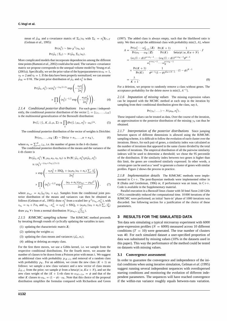
Fig. 5. Four true clusters (left) are compared with the RJMCMC-clusters(right) obtained using a random gene as seed. The dashed line represents thecentroid of the cluster and the solid line the profile of the gene used as seed.Clusters 5–40 can be found in the Supplementary Figures 4–8.

3.3 Clustering of gene-expression profiles withmissing values

The concordance between the clusters of the complete and theincomplete (0.1 missing) datasets is >75% on average (85.07,90.64, 84.42, 89.16, 81.76, 83.29, 86.44, 80.84, 84.22 and 77.62%)for the 10 simulated datasets. See Figure 3 in the Supplementarymaterial for the complete percentages per simulated cluster.

When a random gene is picked from the first four simulatedclusters and the clusters are reconstructed from this seed, highconcordance with the profiles of the true clusters is observed (Fig. 5and Supplementary material).

3.4 Comparison with k-means clusteringThe RJMCMC-based clustering algorithm has the advantage overother clustering methods, e.g. k-means, of allowing the clustering ofgene-expression profiles without advance specification of the numberof clusters. Methods proposed to estimate the number of clusters in agiven dataset are often based on k-fold cross-validation and variantsthereof, e.g. the figure of merit (FOM, Yeung et al., 2001b).

For the simulated data, the results using FOM proved inconclusive(see the Supplementary material). Thus the true number of clusterswas supplied to the k-means algorithm using the academic software‘Genesis’ (Sturn et al., 2002). Its sensitivity and specificity was com-pared with the RJMCMC-based clustering. Since real data almostalways contain missing values, we used the dataset with missingvalues for comparison.

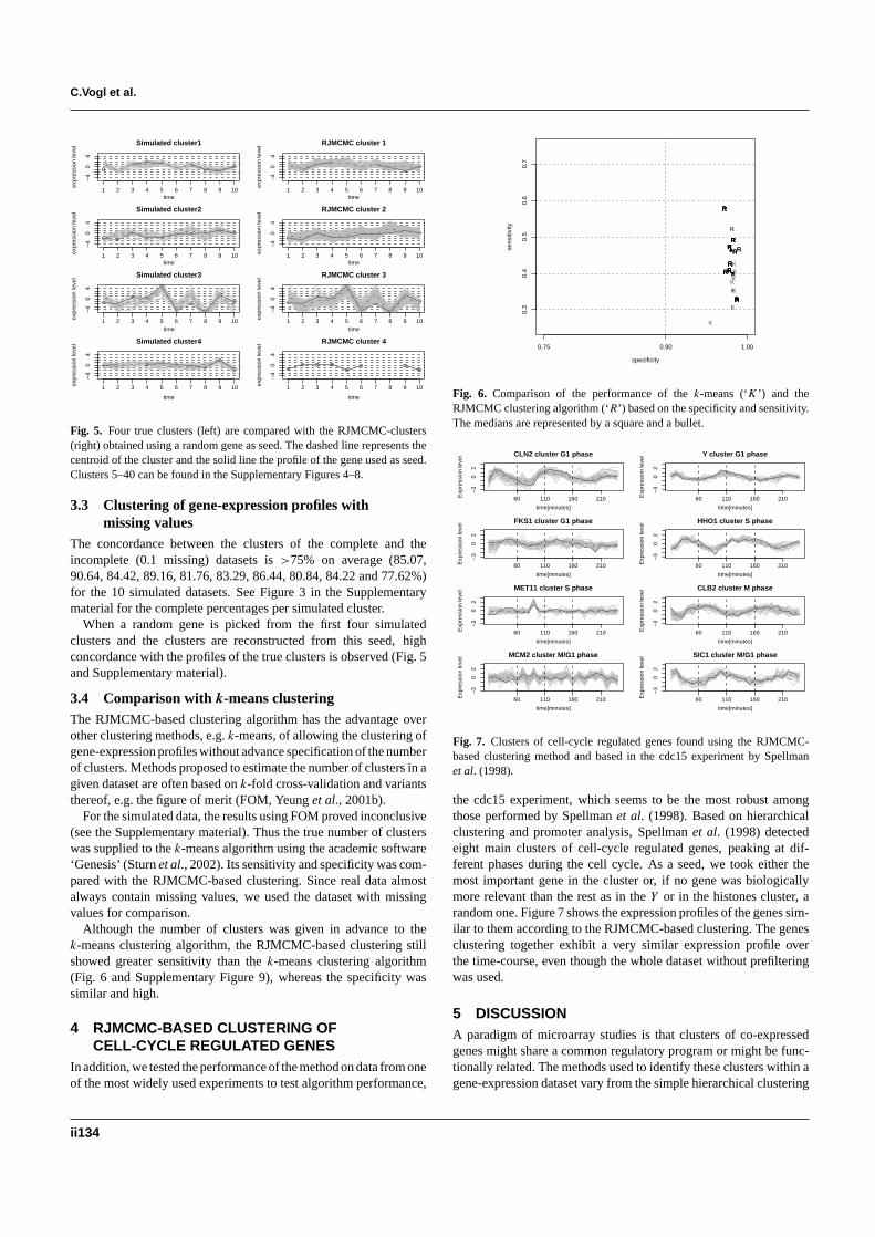
Although the number of clusters was given in advance to thek-means clustering algorithm, the RJMCMC-based clustering stillshowed greater sensitivity than the k-means clustering algorithm(Fig. 6 and Supplementary Figure 9), whereas the specificity wassimilar and high.

4 RJMCMC-BASED CLUSTERING OFCELL-CYCLE REGULATED GENES

In addition, we tested the performance of the method on data from oneof the most widely used experiments to test algorithm performance,

K

specificity

sens

itivi

ty

0.75 0.90 1.00

0.3

0.4

0.5

0.6

0.7

R

K

R

R

K

R

R

R

K

R

R

R

RK

R

R

R

R

R

K

R

R

R

R

R

R

K

R

R

R

R

R

RR

K

R

R

R

R

R

RR

R

K

R

R

R

R

R

RR

RR

K

R

R

R

R

R

RR

RR

R

Fig. 6. Comparison of the performance of the k-means (‘K’) and theRJMCMC clustering algorithm (‘R’) based on the specificity and sensitivity.The medians are represented by a square and a bullet.

time[minutes]

Exp

ress

ion

leve

l

60 110 160 210

–30

2

CLN2 cluster G1 phase

time[minutes]

Exp

ress

ion

leve

l

60 110 160 210

–30

2

Y cluster G1 phase

time[minutes]

Exp

ress

ion

leve

l

60 110 160 210

–30

2

FKS1 cluster G1 phase

time[minutes]

Exp

ress

ion

leve

l

60 110 160 210

–30

2

HHO1 cluster S phase

time[minutes]

Exp

ress

ion

leve

l

60 110 160 210

–30

2

MET11 cluster S phase

time[minutes]E

xpre

ssio

n le

vel

60 110 160 210

–30

2

CLB2 cluster M phase

time[minutes]

Exp

ress

ion

leve

l

60 110 160 210

–30

2

MCM2 cluster M/G1 phase

time[minutes]

Exp

ress

ion

leve

l

60 110 160 210

–30

2SIC1 cluster M/G1 phase

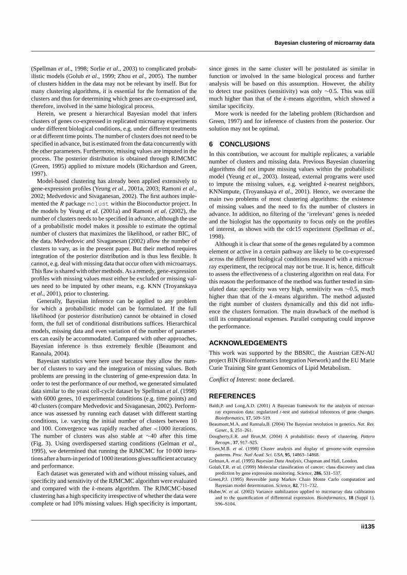
Fig. 7. Clusters of cell-cycle regulated genes found using the RJMCMC-based clustering method and based in the cdc15 experiment by Spellmanet al. (1998).

the cdc15 experiment, which seems to be the most robust amongthose performed by Spellman et al. (1998). Based on hierarchicalclustering and promoter analysis, Spellman et al. (1998) detectedeight main clusters of cell-cycle regulated genes, peaking at dif-ferent phases during the cell cycle. As a seed, we took either themost important gene in the cluster or, if no gene was biologicallymore relevant than the rest as in the Y or in the histones cluster, arandom one. Figure 7 shows the expression profiles of the genes sim-ilar to them according to the RJMCMC-based clustering. The genesclustering together exhibit a very similar expression profile overthe time-course, even though the whole dataset without prefilteringwas used.

5 DISCUSSIONA paradigm of microarray studies is that clusters of co-expressedgenes might share a common regulatory program or might be func-tionally related. The methods used to identify these clusters within agene-expression dataset vary from the simple hierarchical clustering

ii134

Bayesian clustering of microarray data

(Spellman et al., 1998; Sorlie et al., 2003) to complicated probab-ilistic models (Golub et al., 1999; Zhou et al., 2005). The numberof clusters hidden in the data may not be relevant by itself. But formany clustering algorithms, it is essential for the formation of theclusters and thus for determining which genes are co-expressed and,therefore, involved in the same biological process.

Herein, we present a hierarchical Bayesian model that infersclusters of genes co-expressed in replicated microarray experimentsunder different biological conditions, e.g. under different treatmentsor at different time points. The number of clusters does not need to bespecified in advance, but is estimated from the data concurrently withthe other parameters. Furthermore, missing values are imputed in theprocess. The posterior distribution is obtained through RJMCMC(Green, 1995) applied to mixture models (Richardson and Green,1997).

Model-based clustering has already been applied extensively togene-expression profiles (Yeung et al., 2001a, 2003; Ramoni et al.,2002; Medvedovic and Sivaganesan, 2002). The first authors imple-mented the R package mclust within the Bioconductor project. Inthe models by Yeung et al. (2001a) and Ramoni et al. (2002), thenumber of clusters needs to be specified in advance, although the useof a probabilistic model makes it possible to estimate the optimalnumber of clusters that maximizes the likelihood, or rather BIC, ofthe data. Medvedovic and Sivaganesan (2002) allow the number ofclusters to vary, as in the present paper. But their method requiresintegration of the posterior distribution and is thus less flexible. Itcannot, e.g. deal with missing data that occur often with microarrays.This flaw is shared with other methods. As a remedy, gene-expressionprofiles with missing values must either be excluded or missing val-ues need to be imputed by other means, e.g. KNN (Troyanskayaet al., 2001), prior to clustering.

Generally, Bayesian inference can be applied to any problemfor which a probabilistic model can be formulated. If the fulllikelihood (or posterior distribution) cannot be obtained in closedform, the full set of conditional distributions suffices. Hierarchicalmodels, missing data and even variation of the number of paramet-ers can easily be accommodated. Compared with other approaches,Bayesian inference is thus extremely flexible (Beaumont andRannala, 2004).

Bayesian statistics were here used because they allow the num-ber of clusters to vary and the integration of missing values. Bothproblems are pressing in the clustering of gene-expression data. Inorder to test the performance of our method, we generated simulateddata similar to the yeast cell-cycle dataset by Spellman et al. (1998)with 6000 genes, 10 experimental conditions (e.g. time points) and40 clusters (compare Medvedovic and Sivaganesan, 2002). Perform-ance was assessed by running each dataset with different startingconditions, i.e. varying the initial number of clusters between 10and 100. Convergence was rapidly reached after <1000 iterations.The number of clusters was also stable at ∼40 after this time(Fig. 3). Using overdispersed starting conditions (Gelman et al.,1995), we determined that running the RJMCMC for 10 000 itera-tions after a burn-in period of 1000 iterations gives sufficient accuracyand performance.

Each dataset was generated with and without missing values, andspecificity and sensitivity of the RJMCMC algorithm were evaluatedand compared with the k-means algorithm. The RJMCMC-basedclustering has a high specificity irrespective of whether the data werecomplete or had 10% missing values. High specificity is important,

since genes in the same cluster will be postulated as similar infunction or involved in the same biological process and furtheranalysis will be based on this assumption. However, the abilityto detect true positives (sensitivity) was only ∼0.5. This was stillmuch higher than that of the k-means algorithm, which showed asimilar specificity.

More work is needed for the labeling problem (Richardson andGreen, 1997) and for inference of clusters from the posterior. Oursolution may not be optimal.

6 CONCLUSIONSIn this contribution, we account for multiple replicates, a variablenumber of clusters and missing data. Previous Bayesian clusteringalgorithms did not impute missing values within the probabilisticmodel (Yeung et al., 2003). Instead, external programs were usedto impute the missing values, e.g. weighted k-nearest neighbors,KNNimpute, (Troyanskaya et al., 2001). Hence, we overcame themain two problems of most clustering algorithms: the existenceof missing values and the need to fix the number of clusters inadvance. In addition, no filtering of the ‘irrelevant’ genes is neededand the biologist has the opportunity to focus only on the profilesof interest, as shown with the cdc15 experiment (Spellman et al.,1998).

Although it is clear that some of the genes regulated by a commonelement or active in a certain pathway are likely to be co-expressedacross the different biological conditions measured with a microar-ray experiment, the reciprocal may not be true. It is, hence, difficultto assess the effectiveness of a clustering algorithm on real data. Forthis reason the performance of the method was further tested in sim-ulated data: specificity was very high, sensitivity was ∼0.5, muchhigher than that of the k-means algorithm. The method adjustedthe right number of clusters dynamically and this did not influ-ence the clusters formation. The main drawback of the method isstill its computational expenses. Parallel computing could improvethe performance.

ACKNOWLEDGEMENTSThis work was supported by the BBSRC, the Austrian GEN-AUproject BIN (Bioinformatics Integration Network) and the EU MarieCurie Training Site grant Genomics of Lipid Metabolism.

Conflict of Interest: none declared.

REFERENCESBaldi,P. and Long,A.D. (2001) A Bayesian framework for the analysis of microar-

ray expression data: regularized t-test and statistical inferences of gene changes.Bioinformatics, 17, 509–519.

Beaumont,M.A. and Rannala,B. (2004) The Bayesian revolution in genetics. Nat. Rev.Genet., 5, 251–261.

Dougherty,E.R. and Brun,M. (2004) A probabilistic theory of clustering. PatternRecogn., 37, 917–925.

Eisen,M.B. et al. (1998) Cluster analysis and display of genome-wide expressionpatterns. Proc. Natl Acad. Sci. USA, 95, 14863–14868.

Gelman,A. et al. (1995) Bayesian Data Analysis, Chapman and Hall, London.Golub,T.R. et al. (1999) Molecular classification of cancer: class discovery and class

prediction by gene expression monitoring. Science, 286, 531–537.Green,P.J. (1995) Reversible jump Markov Chain Monte Carlo computation and

Bayesian model determination. Science, 82, 711–732.Huber,W. et al. (2002) Variance stabilization applied to microarray data calibration

and to the quantification of differential expression. Bioinformatics, 18 (Suppl 1),S96–S104.

ii135

C.Vogl et al.

Ihaka,R. and Gentleman,R. (1996) R: a language for data analysis and graphics,J. Comput. Graph. Stat., 5, 299–314.

Medvedovic,M. and Sivaganesan,S. (2002) Bayesian infinite mixture model basedclustering of gene expression profiles. Bioinformatics, 18, 1194–1206.

Ramoni,M.F. et al. (2002) Cluster analysis of gene expression dynamics, Proc. NatlAcad. Sci. USA, 99, 9121–9126.

Richardson,S. and Green,P.J. (1997) On Bayesian analysis of mixtures with an unknownnumber of components. J. R. Stat. Soc., 59, 731–792.

Schwarz,G. (1978) Estimating the dimension of a model. Ann. Stat., 6, 461–464.Segal,E. et al. (2003) Decomposing gene expression into cellular processes. Pac. Symp.

Biocomput., 89–100.Sorlie,T. et al. (2003) Repeated observation of breast tumor subtypes in

independent gene expression data sets. Proc. Natl Acad. Sci. USA, 100,8418–8423.

Spellman,P.T. et al. (1998) Comprehensive identification of cell cycle-regulated genesof the yeast Saccharomices cerevisae by microarray hybridization. Mol. Biol. Cell,9, 3273–3297.

Sturn,A. et al. (2002) Genesis: cluster analysis of microarray data. Bioinformatics, 18,207–208.

Tamayo,P. et al. (1999) Interpreting patterns of gene expression with self-organizingmaps: methods and application to hematopoietic differentiation. Proc. Natl Acad.Sci. USA, 96, 2907–2912.

Tavazoie,S. et al. (1999) Systematic determination of genetic network architecture.Nat. Genet., 22, 281–285.

Troyanskaya,O. et al. (2001) Missing value estimation methods for DNA microarrays.Bioinformatics, 17, 520–525.

Yeung,K.Y. et al. (2001a) Model-based clustering and data transformations for geneexpression data. Bioinformatics, 17, 977–987.

Yeung,K.Y. et al. (2001b) Validating clustering for gene expression data. Bioinformatics,17, 309–318.

Yeung,K.Y. et al. (2003) Clustering gene-expression data with repeated measurements.Genome Biol., 4, R34.

Zhou,X.J. et al. (2005) Functional annotation and network reconstruction through cross-platform integration of microarray data. Nat. Biotechnol., 23, 238–243.

ii136